Embed Size (px)
Citation preview
1
Molecular Motion
Dr Yimin Chao Room 1.45
Email: [email protected]://www.uea.ac.uk/~qwn07jsu
CHE-1H26: Elements of Chemical Physics
2
Outline• 1. Transport properties• 2. Diffusion and viscosity• 2.1 Diffusion process• 2.2 Viscosity• 3. The relationship of diffusion and viscosity– Einstein-Stokes relationship• 4. The effects of temperature on viscosity and diffusion—Arrhenius Law• 5. Methods of measurement• 6. Rotational diffusion• 7. using viscosity and diffusion to measure the shapes and sizes of molecules
References:• Atkins's Physical Chemistry, 8th Ed, P Atkins and J de Paulo,2002,OUP.• Elements of Physical Chemistry, 5th Ed, P Atkins and J de Paulo,2009,OUP• University Physics, 12th Ed, F Sears, MW Zemansky and HD Young, 2000,
Addison and Welsey.
3
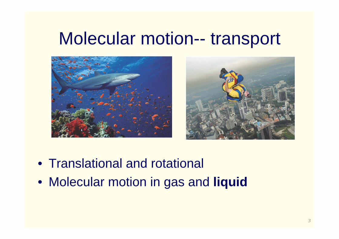
Molecular motion-- transport
• Translational and rotational• Molecular motion in gas and liquid
4
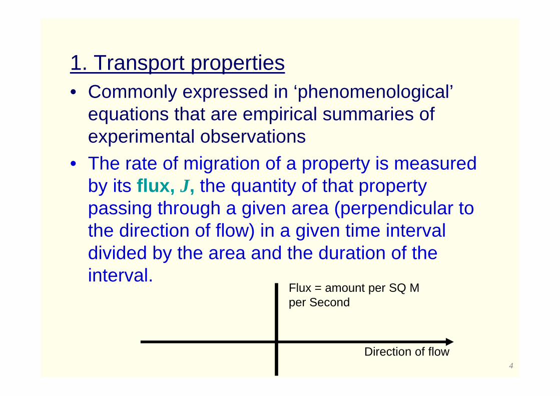
1. Transport properties• Commonly expressed in ‘phenomenological’
equations that are empirical summaries of experimental observations
• The rate of migration of a property is measured by its flux, J, the quantity of that property passing through a given area (perpendicular to the direction of flow) in a given time interval divided by the area and the duration of the interval.
Direction of flow
Flux = amount per SQ M per Second
5
In general the flux J is proportional to the gradient, X, causing the flux
L– proportionality constant
• Both flux and gradient are VECTORS they have both sign and magnitude.
• The flux acts in a direction such that it reduces the gradient.
Flux
XLJrr
=
6
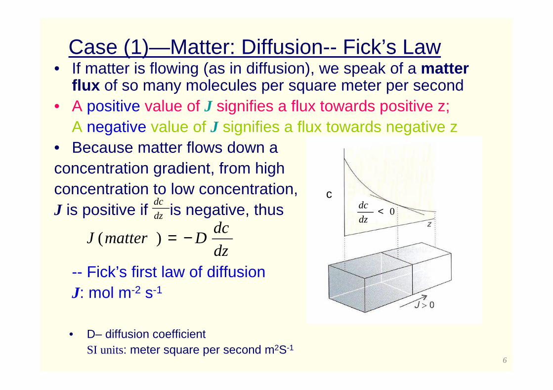
Case (1)—Matter: Diffusion-- Fick’s Law• If matter is flowing (as in diffusion), we speak of a matter
flux of so many molecules per square meter per second• A positive value of J signifies a flux towards positive z;
A negative value of J signifies a flux towards negative z• Because matter flows down a concentration gradient, from high concentration to low concentration, J is positive if is negative, thus
-- Fick’s first law of diffusionJ: mol m-2 s-1
dz
dcDmatterJ −=)(
dz
dc dc/dzc
0<dz
dc
• D– diffusion coefficientSI units: meter square per second m2S-1
7
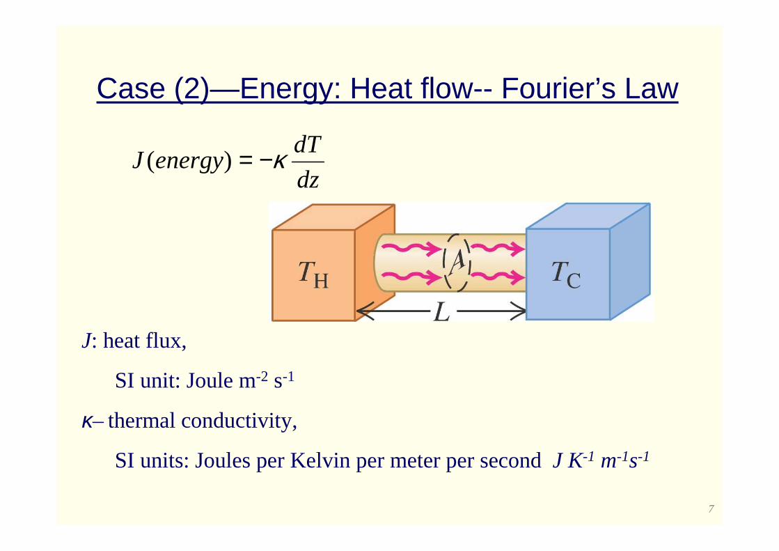
Case (2)—Energy: Heat flow-- Fourier’s Law
dz
dTenergyJ κ−=)(
J: heat flux,
SI unit: Joule m-2 s-1
κ– thermal conductivity,
SI units: Joules per Kelvin per meter per second J K-1 m-1s-1
8
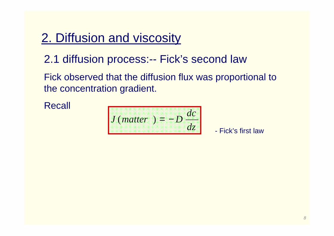
2. Diffusion and viscosity
2.1 diffusion process:-- Fick’s second law
Fick observed that the diffusion flux was proportional to the concentration gradient.
Recall
dz
dcDmatterJ −=)(
- Fick’s first law
9
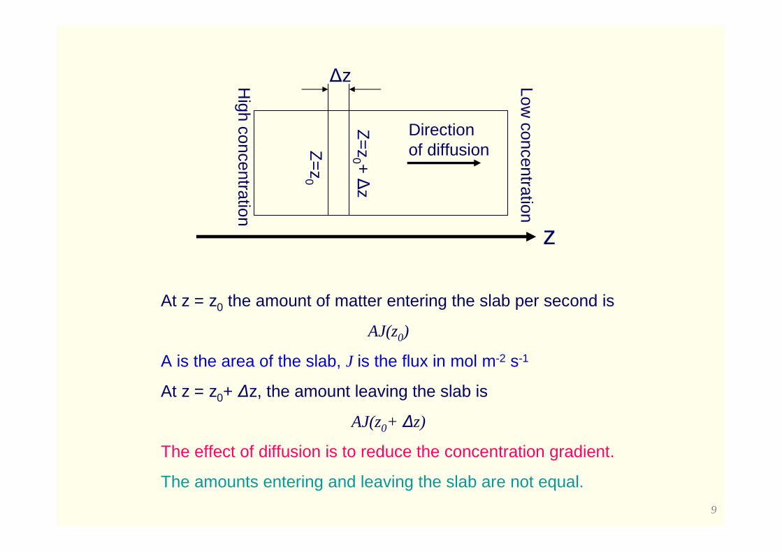
z
Direction of diffusion
∆z
Z=
z0
Z=
z0 +
∆z
High concentration
Low concentration
At z = z0 the amount of matter entering the slab per second is
AJ(z0)
A is the area of the slab, J is the flux in mol m-2 s-1
At z = z0+ ∆z, the amount leaving the slab is
AJ(z0+ ∆z)
The effect of diffusion is to reduce the concentration gradient.
The amounts entering and leaving the slab are not equal.
10
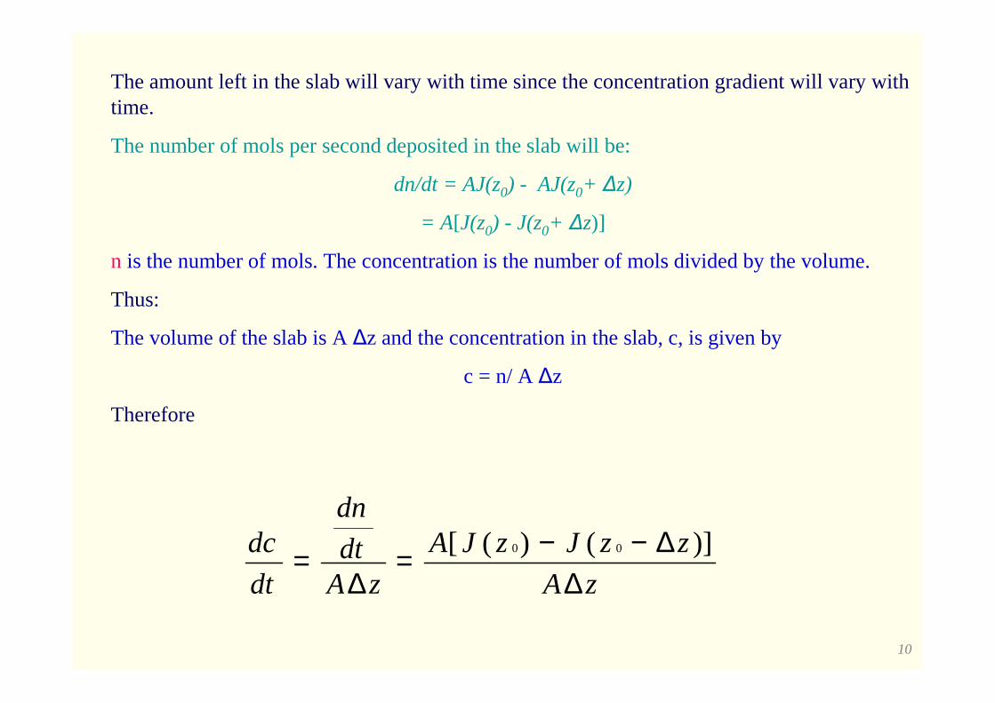
The amount left in the slab will vary with time since the concentration gradient will vary with time.
The number of mols per second deposited in the slab will be:
dn/dt = AJ(z0) - AJ(z0+ ∆z)
= A[J(z0) - J(z0+ ∆z)]
n is the number of mols. The concentration is the number of mols divided by the volume.
Thus:
The volume of the slab is A ∆z and the concentration in the slab, c, is given by
c = n/ A ∆z
Therefore
zA
zzJzJA
zAdt
dn
dt
dc
∆∆−−=
∆= )]()([ 00
11
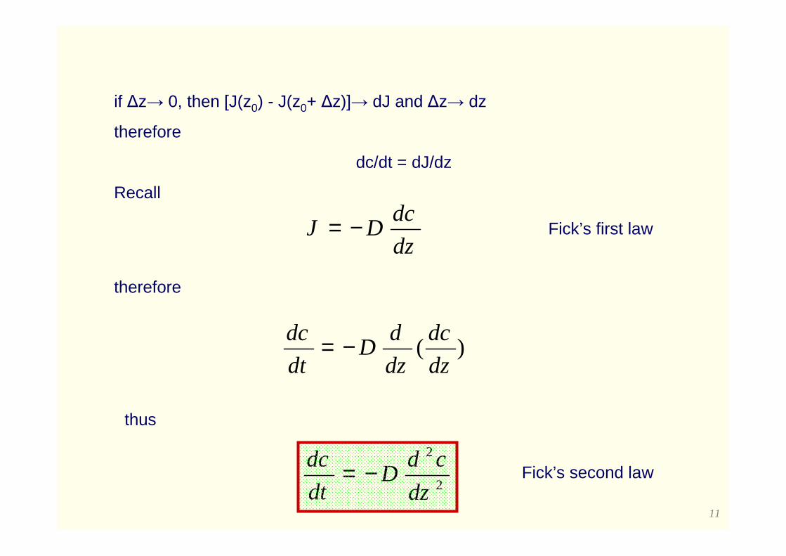
if ∆z→ 0, then [J(z0) - J(z0+ ∆z)]→ dJ and ∆z→ dz
therefore
dc/dt = dJ/dz
Recall
dz
dcDJ −=
therefore
)(dz
dc
dz
dD
dt
dc −=
thus
2
2
dz
cdD
dt
dc −=
Fick’s first law
Fick’s second law
12
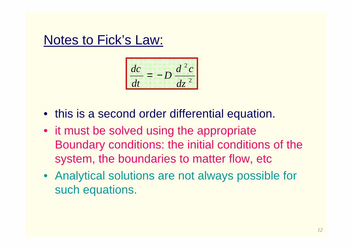
Notes to Fick’s Law:
• this is a second order differential equation.• it must be solved using the appropriate
Boundary conditions: the initial conditions of the system, the boundaries to matter flow, etc
• Analytical solutions are not always possible for such equations.
2
2
dz
cdD
dt
dc −=
13
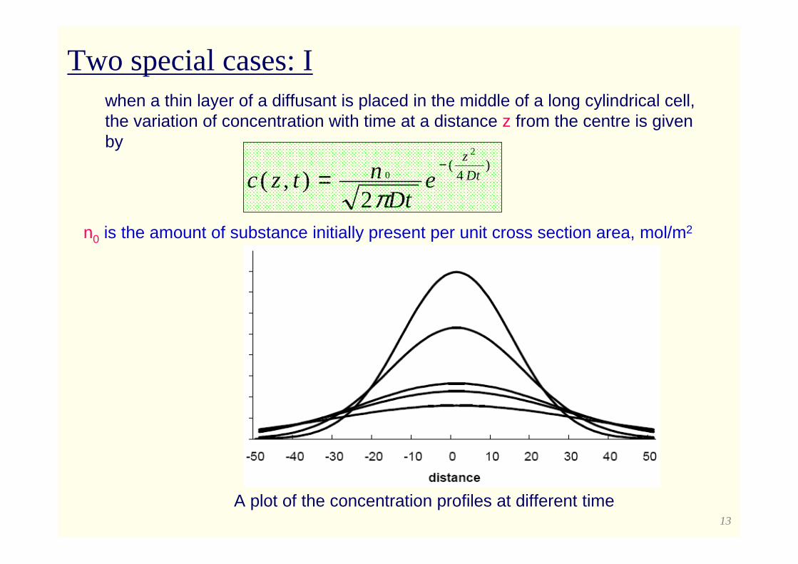
when a thin layer of a diffusant is placed in the middle of a long cylindrical cell, the variation of concentration with time at a distance z from the centre is given by
)4
(2
0
2),( Dt
z
eDt
ntzc−
=π
n0 is the amount of substance initially present per unit cross section area, mol/m2
A plot of the concentration profiles at different time
Two special cases: I
14
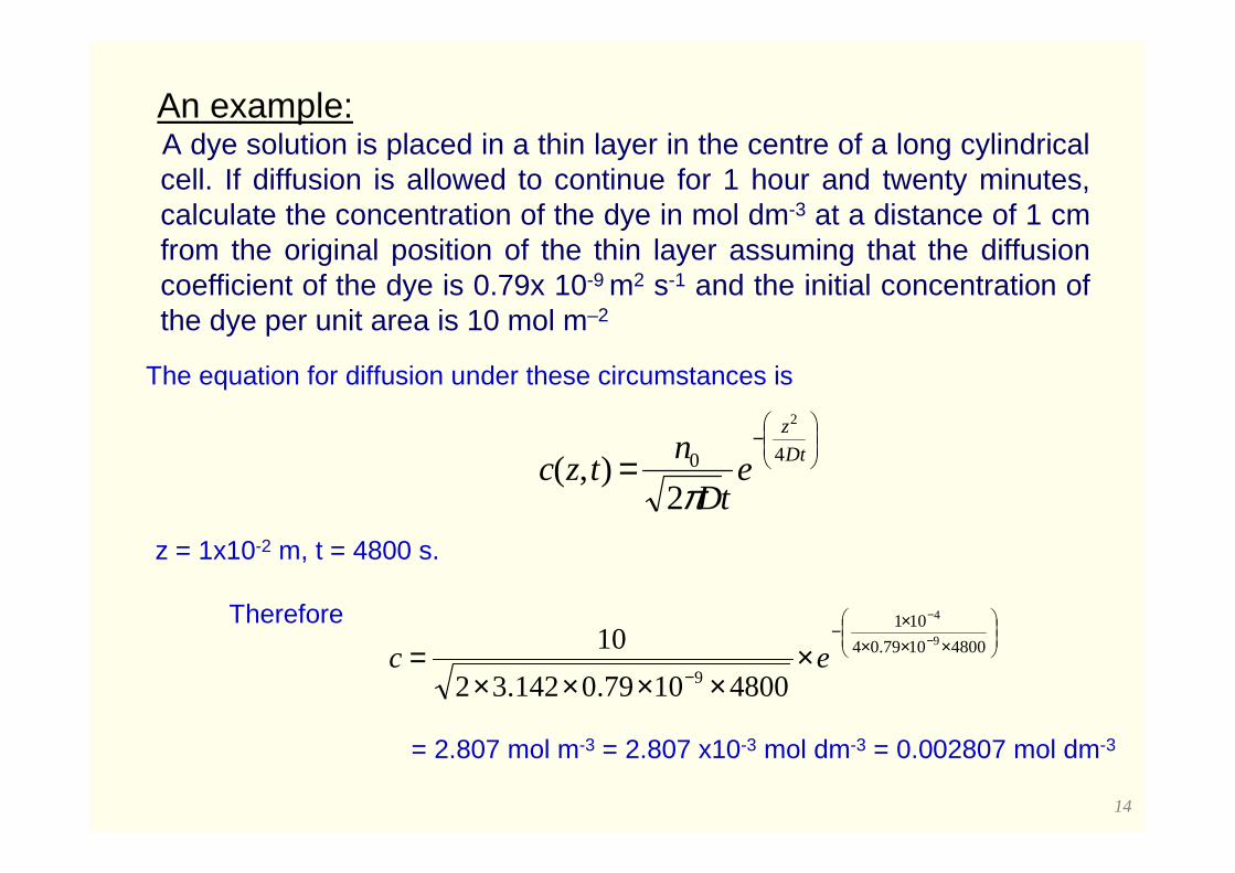
An example:A dye solution is placed in a thin layer in the centre of a long cylindrical cell. If diffusion is allowed to continue for 1 hour and twenty minutes, calculate the concentration of the dye in mol dm-3 at a distance of 1 cm from the original position of the thin layer assuming that the diffusion coefficient of the dye is 0.79x 10⁻⁹ m2 s-1 and the initial concentration of the dye per unit area is 10 mol m–2
The equation for diffusion under these circumstances is
−
= Dt
z
etD
ntzc
40
2
2),(
πz = 1x10⁻² m, t = 4800 s.
Therefore
××××−
−
−
−
×××××
= 48001079.04
101
9
9
4
48001079.0142.32
10ec
= 2.807 mol m-3 = 2.807 x10⁻³ mol dm-3 = 0.002807 mol dm-3

15
0
50
100
150
200
250
300
350
400
-60 -40 -20 0 20 40 60
020406080
100120140160180
-60 -40 -20 0 20 40 60
0
10
20
30
40
50
60
70
-60 -40 -20 0 20 40 60
0
5
10
15
20
25
-60 -40 -20 0 20 40 60
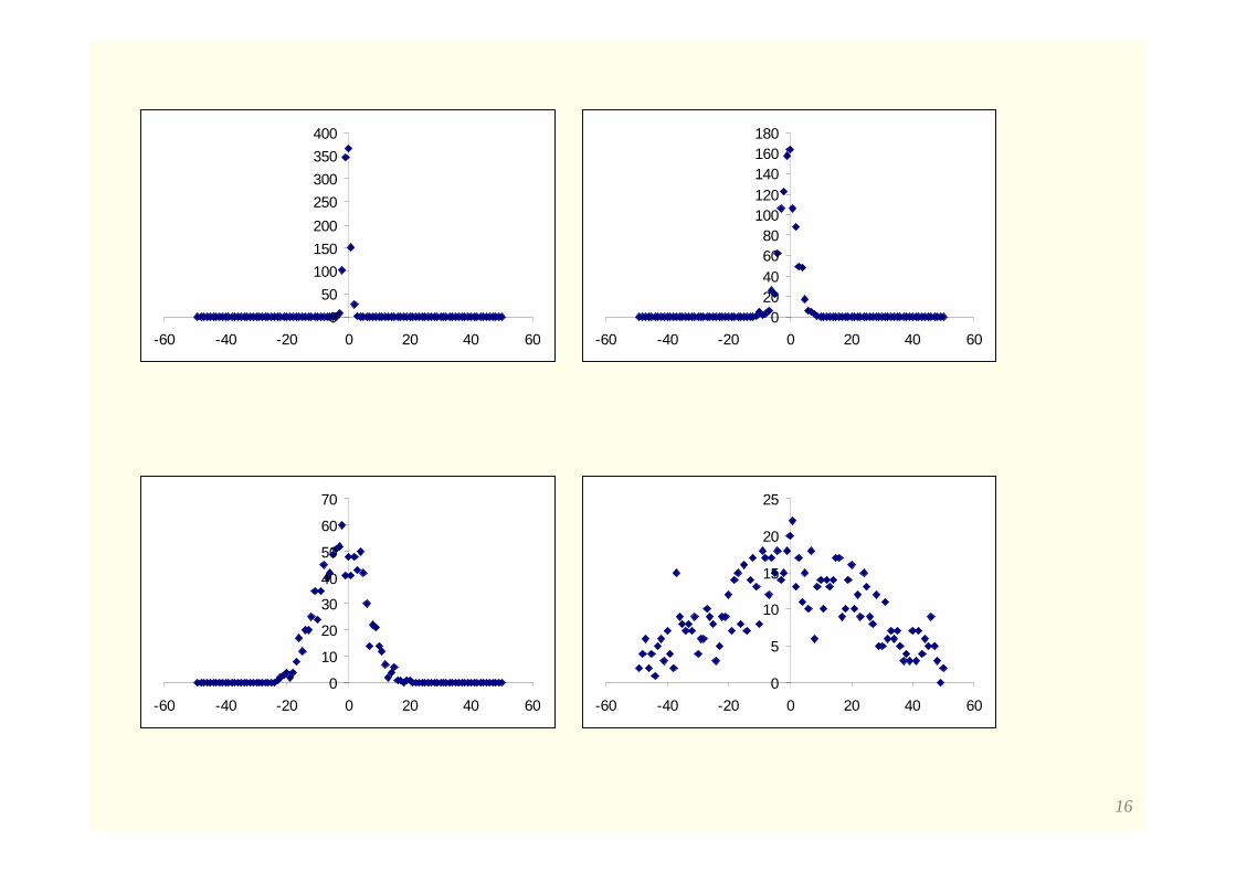
A simulated result:
16
0
50
100
150
200
250
300
350
400
-60 -40 -20 0 20 40 60
020406080
100120140160180
-60 -40 -20 0 20 40 60
0
10
20
30
40
50
60
70
-60 -40 -20 0 20 40 60
0
5
10
15
20
25
-60 -40 -20 0 20 40 60
17
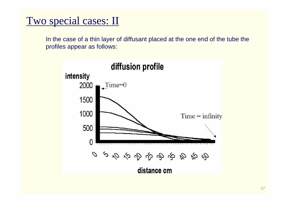
In the case of a thin layer of diffusant placed at the one end of the tube the profiles appear as follows:
Two special cases: II
18
2.2 Viscosity
r ry
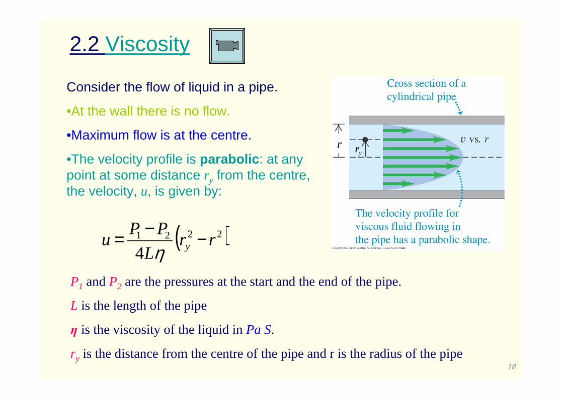
Consider the flow of liquid in a pipe.
•At the wall there is no flow.
•Maximum flow is at the centre.
•The velocity profile is parabolic : at any point at some distance ry from the centre, the velocity, u, is given by:
( )2221
4rr
L
PPu y −−=
ηP1 and P2 are the pressures at the start and the end of the pipe.
L is the length of the pipe
η is the viscosity of the liquid in Pa S.
ry is the distance from the centre of the pipe and r is the radius of the pipe
19
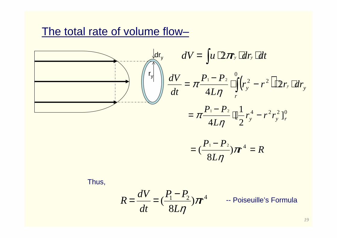
The total rate of volume flow–
ry
dry
421 )8
( rL
PP
dt
dVR π
η−==
dtdrrudV yy ⋅⋅⋅= ∫ π2
Thus,
-- Poiseuille’s Formula
( ) y
r
y drrrrL
PP
dt
dVy ⋅⋅−⋅−= ∫ 2
4
02221
ηπ
0224 ]2
1[
4
21
ryy rrrL
PP −⋅−=η
π
RrL
PP =−= 4)8
(21 π
η
20
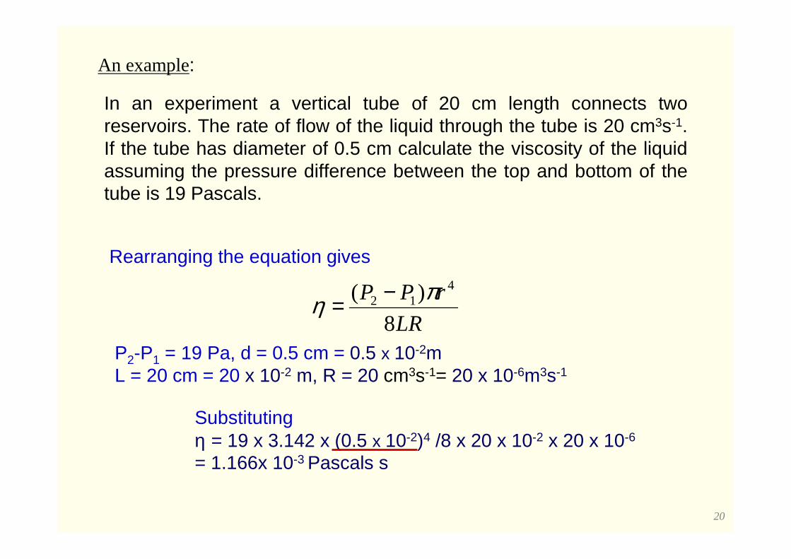
An example:
In an experiment a vertical tube of 20 cm length connects two reservoirs. The rate of flow of the liquid through the tube is 20 cm3s-1. If the tube has diameter of 0.5 cm calculate the viscosity of the liquid assuming the pressure difference between the top and bottom of the tube is 19 Pascals.
Rearranging the equation gives
LR
rPP
8
)( 412 πη −=
Substitutingη = 19 x 3.142 x (0.5 x 10-2)4 /8 x 20 x 10-2 x 20 x 10-6
= 1.166x 10⁻³ Pascals s
P2-P1 = 19 Pa, d = 0.5 cm = 0.5 x 10⁻²mL = 20 cm = 20 x 10-2 m, R = 20 cm3s-1= 20 x 10-6m3s-1
21
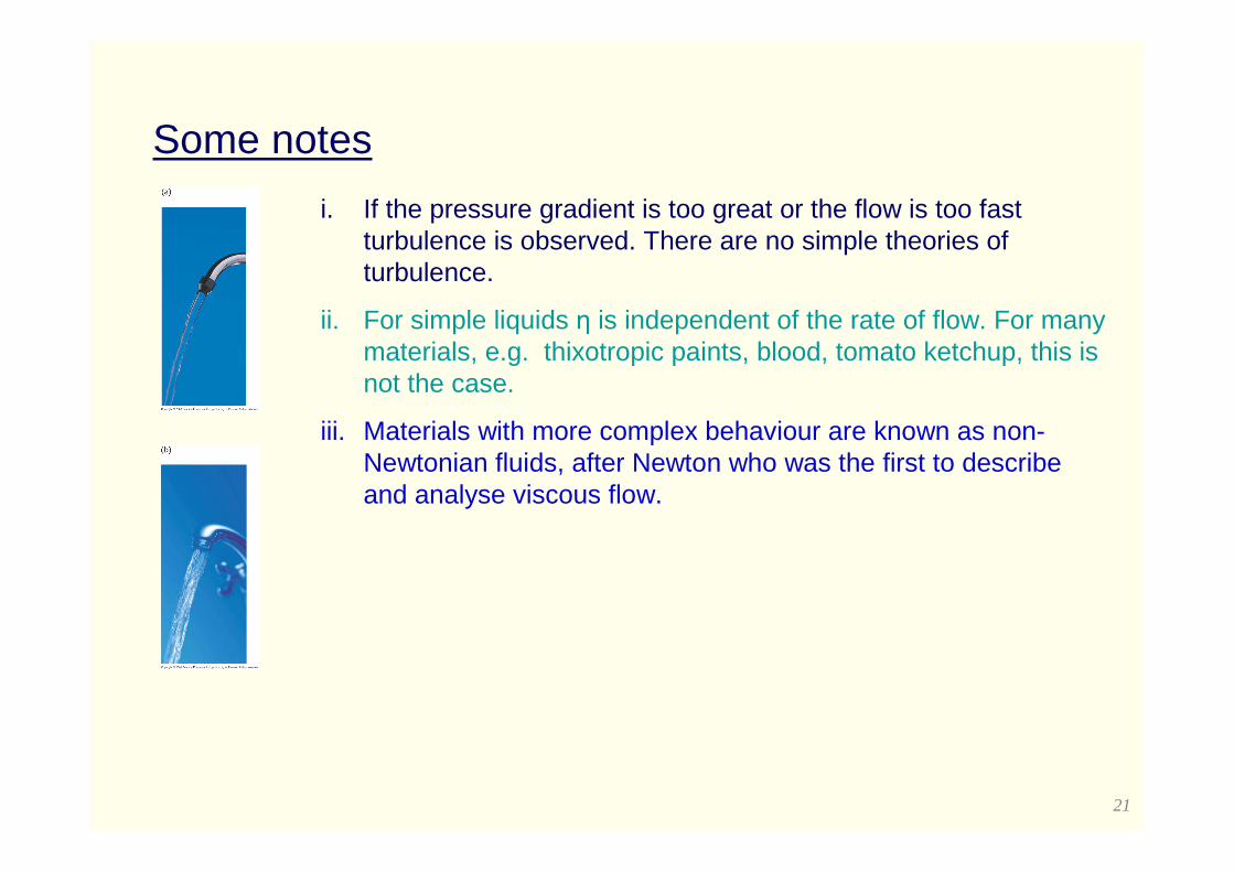
Some notes
i. If the pressure gradient is too great or the flow is too fast turbulence is observed. There are no simple theories of turbulence.
ii. For simple liquids η is independent of the rate of flow. For many materials, e.g. thixotropic paints, blood, tomato ketchup, this is not the case.
iii. Materials with more complex behaviour are known as non-Newtonian fluids, after Newton who was the first to describe and analyse viscous flow.
23
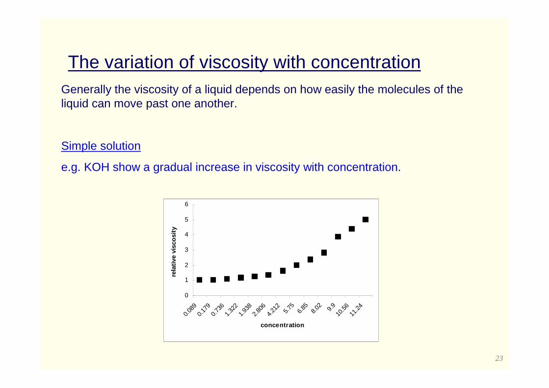
The variation of viscosity with concentrationGenerally the viscosity of a liquid depends on how easily the molecules of the liquid can move past one another.
Simple solution
e.g. KOH show a gradual increase in viscosity with concentration.
0
1
2
3
4
5
6
0.08
90.
179
0.73
61.
322
1.93
82.
806
4.21
25.7
56.8
58.0
2
9.910
.56
11.2
4
concentration
rela
tive
visc
osity
24
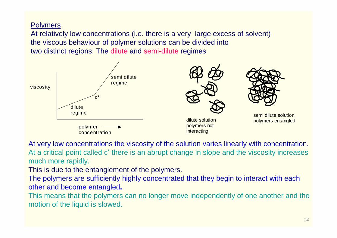
PolymersAt relatively low concentrations (i.e. there is a very large excess of solvent) the viscous behaviour of polymer solutions can be divided into two distinct regions: The dilute and semi-dilute regimes
polymer concentration
viscosity
semi dilute regime
dilute regime
c*
At very low concentrations the viscosity of the solution varies linearly with concentration. At a critical point called c* there is an abrupt change in slope and the viscosity increases much more rapidly.This is due to the entanglement of the polymers. The polymers are sufficiently highly concentrated that they begin to interact with each other and become entangled. This means that the polymers can no longer move independently of one another and the motion of the liquid is slowed.
dilute solution polymers not interacting
semi dilute solution polymers entangled
25
Outline
• 1. Transport properties• 2. Diffusion and viscosity• 2.1 Diffusion process• 2.2 Viscosity• 3. The relationship of diffusion and viscosity–
Einstein-Stokes relationship• 4. The effects of temperature on viscosity and
diffusion—Arrhenius Law• *5. Methods of measurement• 6. Rotational diffusion
26
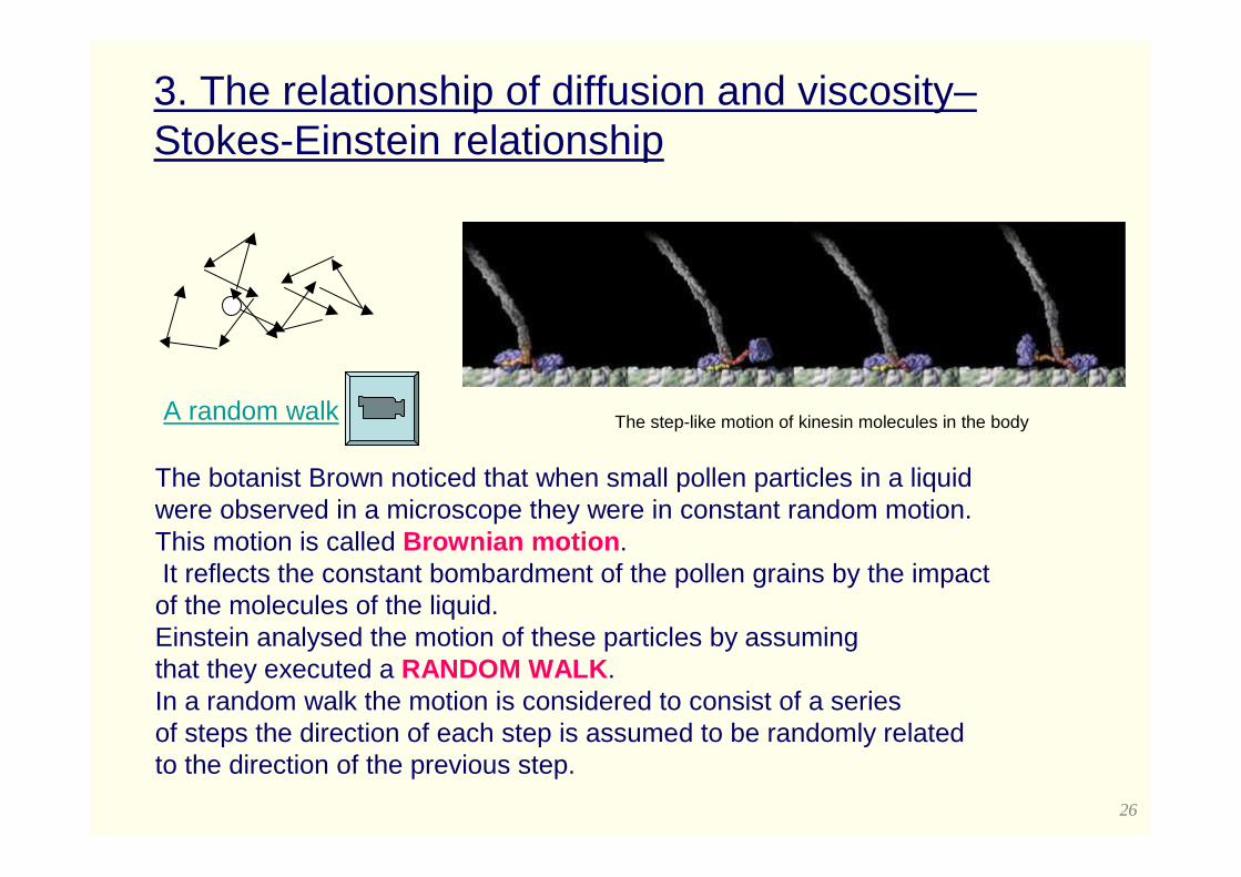
3. The relationship of diffusion and viscosity–Stokes-Einstein relationship
The botanist Brown noticed that when small pollen particles in a liquid were observed in a microscope they were in constant random motion. This motion is called Brownian motion .It reflects the constant bombardment of the pollen grains by the impact
of the molecules of the liquid.Einstein analysed the motion of these particles by assuming that they executed a RANDOM WALK .In a random walk the motion is considered to consist of a seriesof steps the direction of each step is assumed to be randomly related to the direction of the previous step.
A random walk The step-like motion of kinesin molecules in the body
27
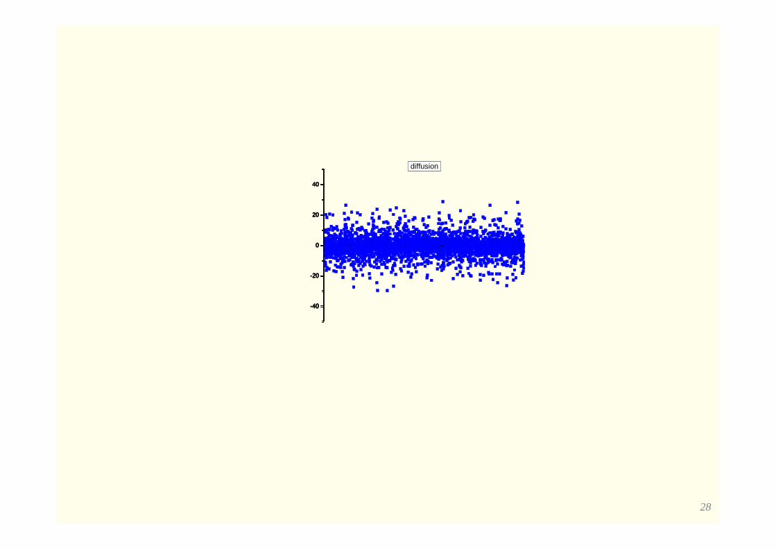
Mutual and self diffusion
Fick’s law is written for a situation in which a concentration gradient exists.It is about the rate of change of the concentration gradient.
The diffusion coefficient is thus the MUTUAL diffusion coefficient and is strictly valid only under defined conditions of concentration gradient. It is the measure of the rate at which one substance diffuses into another.
Brownian motion shows that diffusion can still go on even when there is no concentration gradient. SELF DIFFUSION a measure of the random thermal motion of the molecules in the absence of a concentration gradient.All diffusion arises because of the constant random thermal motion of molecules.
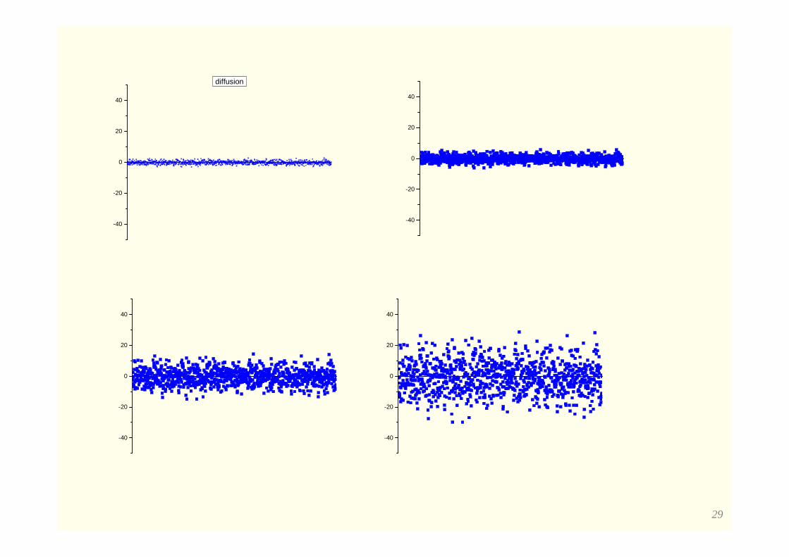
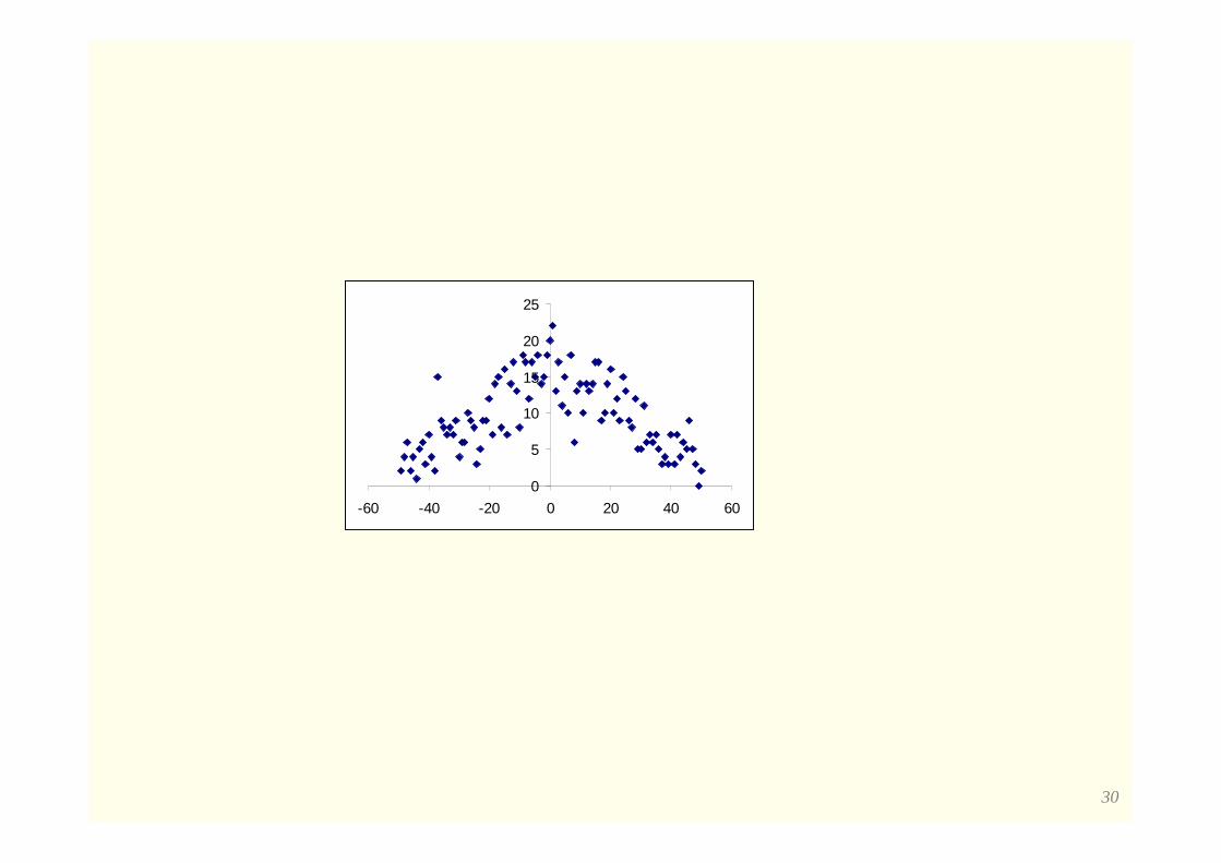
A simulation of diffusion due to random motion is shown below.
28
-40
-20
0
20
40
-40
-20
0
20
40
diffusion
-40
-20
0
20
40
-40
-20
0
20
40
29
-40
-20
0
20
40
-40
-20
0
20
40
diffusion
-40
-20
0
20
40
-40
-20
0
20
40
30
0
50
100
150
200
250
300
350
400
-60 -40 -20 0 20 40 60
020406080
100120140160180
-60 -40 -20 0 20 40 60
0
10
20
30
40
50
60
70
-60 -40 -20 0 20 40 60
0
5
10
15
20
25
-60 -40 -20 0 20 40 60

31
0
50
100
150
200
250
300
350
400
-60 -40 -20 0 20 40 60
020406080
100120140160180
-60 -40 -20 0 20 40 60
0
10
20
30
40
50
60
70
-60 -40 -20 0 20 40 60
0
5
10
15
20
25
-60 -40 -20 0 20 40 60
32
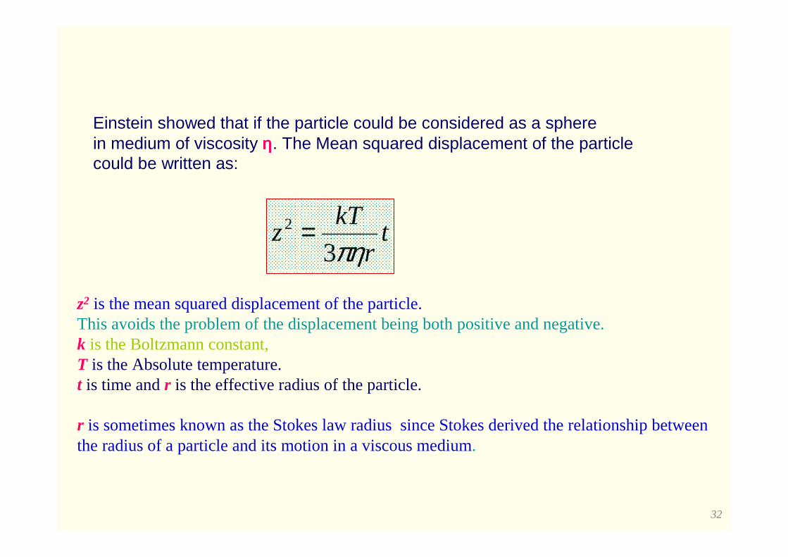
Einstein showed that if the particle could be considered as a sphere in medium of viscosity ηηηη. The Mean squared displacement of the particle could be written as:
tr
kTz
πη32 =
z2 is the mean squared displacement of the particle.This avoids the problem of the displacement being both positive and negative.k is the Boltzmann constant,T is the Absolute temperature. t is time and r is the effective radius of the particle.
r is sometimes known as the Stokes law radius since Stokes derived the relationship between the radius of a particle and its motion in a viscous medium.
33
r
kTD
πη6=
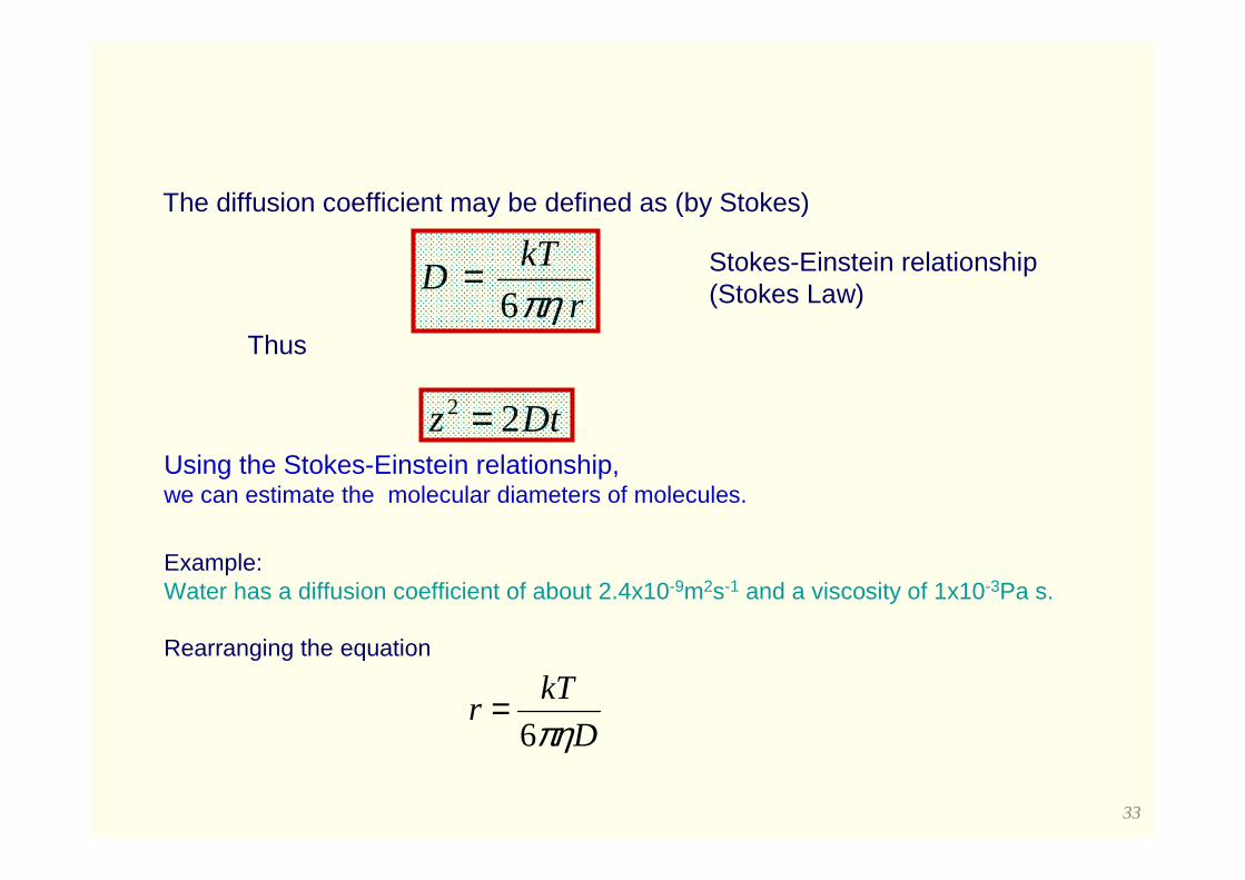
Dtz 22 =
Thus
The diffusion coefficient may be defined as (by Stokes)
Stokes-Einstein relationship(Stokes Law)
Using the Stokes-Einstein relationship, we can estimate the molecular diameters of molecules.
Example:Water has a diffusion coefficient of about 2.4x10⁻⁹m2s-1 and a viscosity of 1x10⁻³Pa s.
Rearranging the equation
D
kTr
πη6=
34
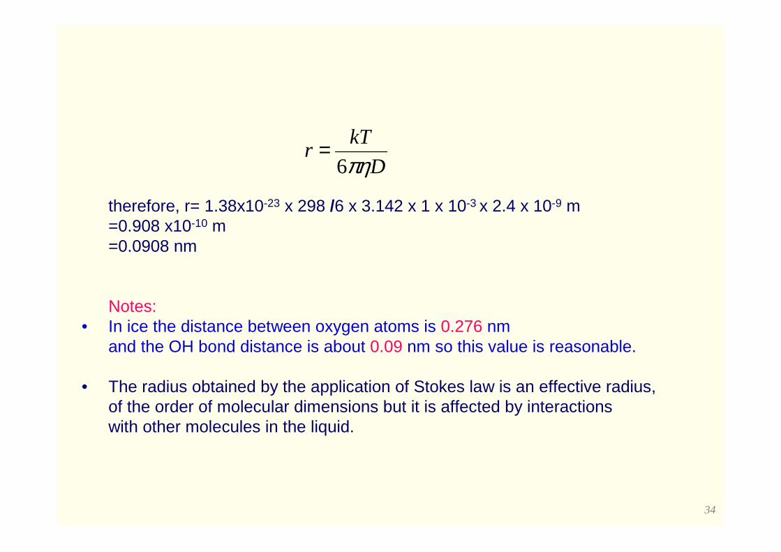
therefore, r= 1.38x10-23 x 298 /6 x 3.142 x 1 x 10-3 x 2.4 x 10-9 m=0.908 x10⁻¹⁰ m=0.0908 nm
Notes: • In ice the distance between oxygen atoms is 0.276 nm
and the OH bond distance is about 0.09 nm so this value is reasonable.
• The radius obtained by the application of Stokes law is an effective radius, of the order of molecular dimensions but it is affected by interactions with other molecules in the liquid.
D
kTr
πη6=
35
DIFFUSION VS VISCOSITY IN SUCROSE
0
2
4
6
8
10
12
14
16
18
0 0.2 0.4 0.6 0.8
RECIPROCAL VISCOSITY
RE
LAT
IVE
DIF
FU
SIO
N C
OE
FF
WATER
SUCROSE
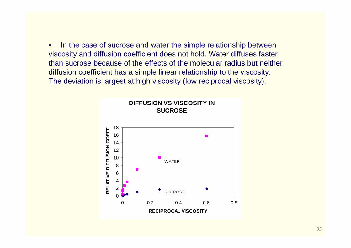
• In the case of sucrose and water the simple relationship betweenviscosity and diffusion coefficient does not hold. Water diffuses faster than sucrose because of the effects of the molecular radius but neither diffusion coefficient has a simple linear relationship to the viscosity. The deviation is largest at high viscosity (low reciprocal viscosity).
36
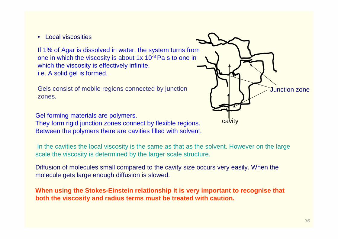
• Local viscosities
If 1% of Agar is dissolved in water, the system turns from one in which the viscosity is about 1x 10⁻³ Pa s to one in which the viscosity is effectively infinite. i.e. A solid gel is formed.
Gels consist of mobile regions connected by junction zones.
Junction zone
cavityGel forming materials are polymers. They form rigid junction zones connect by flexible regions. Between the polymers there are cavities filled with solvent.
In the cavities the local viscosity is the same as that as the solvent. However on the large scale the viscosity is determined by the larger scale structure.
Diffusion of molecules small compared to the cavity size occurs very easily. When the molecule gets large enough diffusion is slowed.
When using the Stokes-Einstein relationship it is v ery important to recognise that both the viscosity and radius terms must be treated with caution.
37
Outline
• 1. Transport properties• 2. Diffusion and viscosity• 2.1 Diffusion process• 2.2 Viscosity• 3. The relationship of diffusion and viscosity– Einstein-
Stokes relationship• 4. The effects of temperature on viscosity and diffusion—
Arrhenius Law• *5. Methods of measurement• 6. Rotational diffusion• 7. using viscosity and diffusion to measure the shapes
and sizes of molecules
38
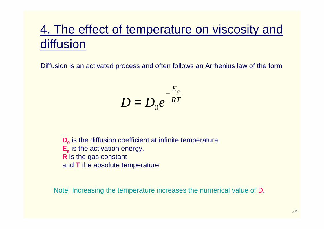
4. The effect of temperature on viscosity and diffusion
Diffusion is an activated process and often follows an Arrhenius law of the form
RT
Ea
eDD−
= 0
D0 is the diffusion coefficient at infinite temperature, Ea is the activation energy, R is the gas constant and T the absolute temperature
Note: Increasing the temperature increases the numerical value of D.
39
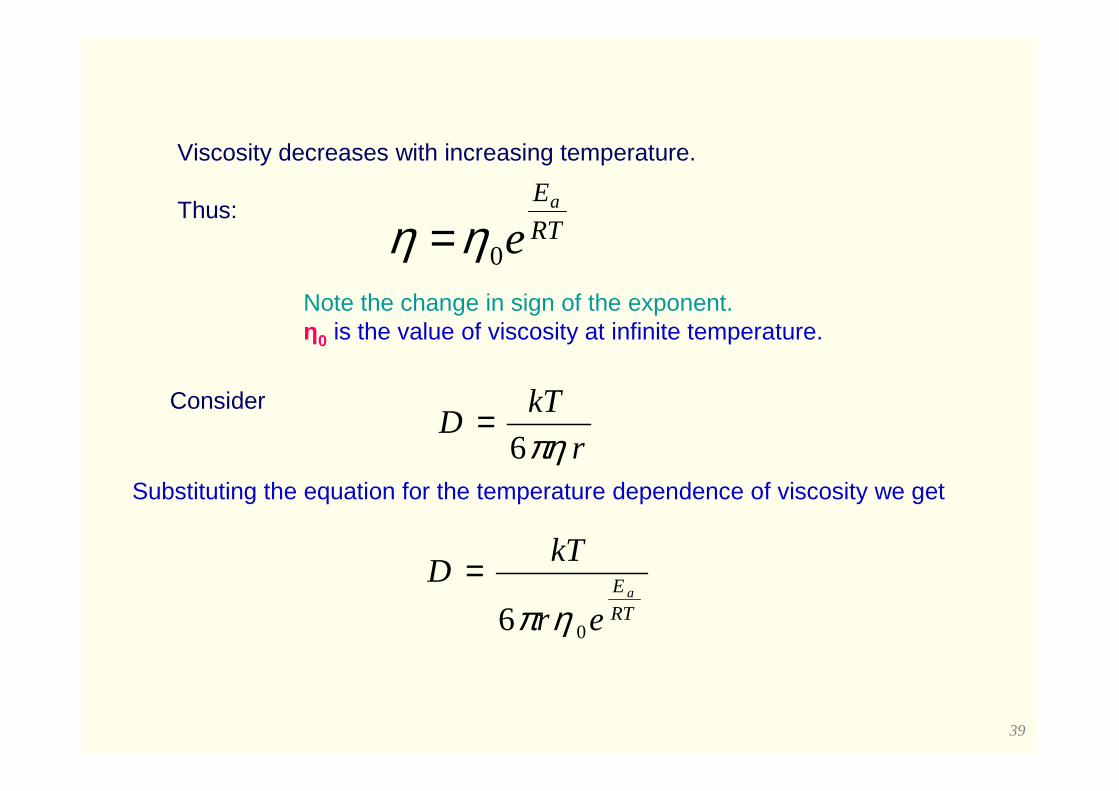
Viscosity decreases with increasing temperature.
Thus:RT
Ea
e0ηη =Note the change in sign of the exponent.η0 is the value of viscosity at infinite temperature.
Consider
r
kTD
πη6=
Substituting the equation for the temperature dependence of viscosity we get
RT
E a
er
kTD
06 ηπ=
40
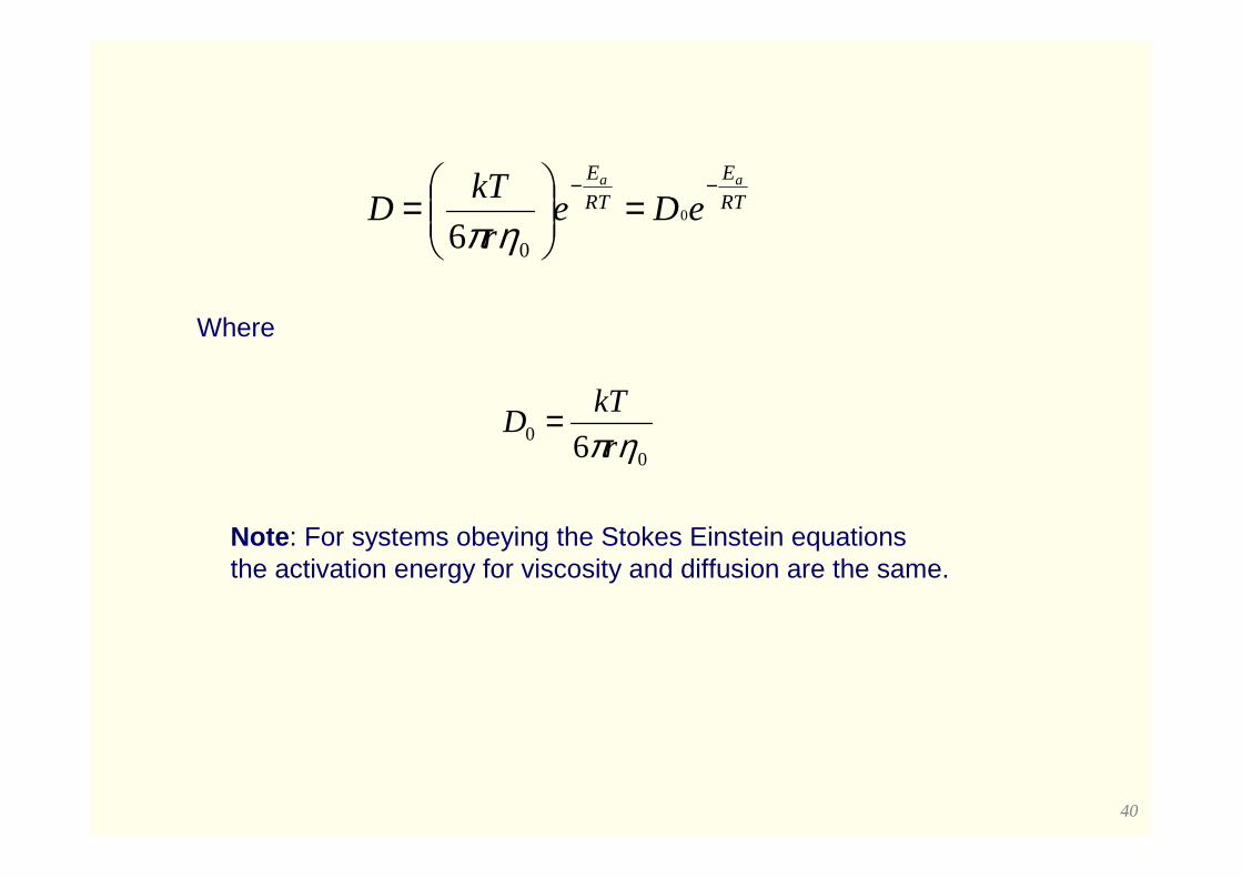
RT
E
RT
E aa
eDer
kTD
−−=
= 0
06 ηπ
Where
00 6 ηπr
kTD =
Note : For systems obeying the Stokes Einstein equations the activation energy for viscosity and diffusion are the same.
41
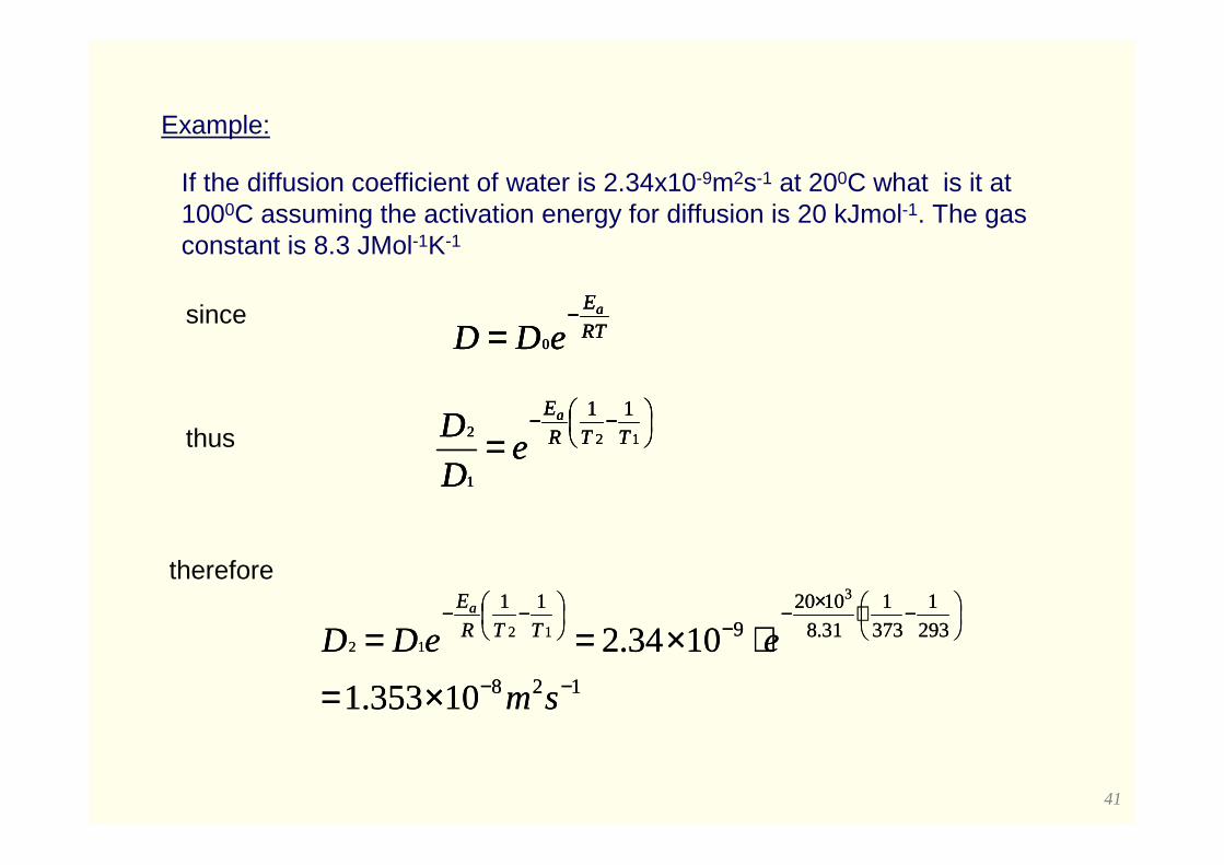
Example:
If the diffusion coefficient of water is 2.34x10⁻⁹m2s-1 at 200C what is it at 1000C assuming the activation energy for diffusion is 20 kJmol-1. The gas constant is 8.3 JMol-1K-1
RT
Ea
eDD−
= 0
−−= 12
1
2
11
TTR
Ea
eD
D
128
293
1
373
1
31.8
10209
11
10353.1
1034.2
3
1212
−−
−⋅×−−
−−
×=
⋅×==
sm
eeDD TTR
Ea
since
thus
therefore
RT
Ea
eDD−
= 0
−−= 12
1
2
11
TTR
Ea
eD
D
128
293
1
373
1
31.8
10209
11
10353.1
1034.2
3
1212
−−
−⋅×−−
−−
×=
⋅×==
sm
eeDD TTR
Ea
RT
Ea
eDD−
= 0
−−= 12
1
2
11
TTR
Ea
eD
D
42
Outline
• 1. Transport properties• 2. Diffusion and viscosity• 2.1 Diffusion process• 2.2 Viscosity• 3. The relationship of diffusion and viscosity– Einstein-
Stokes relationship• 4. The effects of temperature on viscosity and diffusion—
Arrhenius Law• 5. Methods of measurement• 6. Rotational diffusion• 7. using viscosity and diffusion to measure the shapes
and sizes of molecules
43
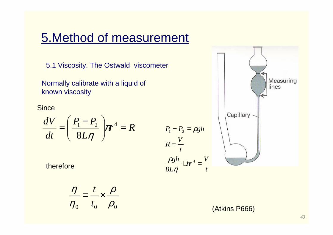
5.Method of measurement
5.1 Viscosity. The Ostwald viscometer
Normally calibrate with a liquid of known viscosity
RrL
PP
dt
dV =
−= 421
8π
η
000 ρρ
ηη ×=
t
t
therefore
(Atkins P666)
t
Vr
L
ght
VR
ghPP
=⋅
=
=−
4
21
8π
ηρ
ρ
Since
44
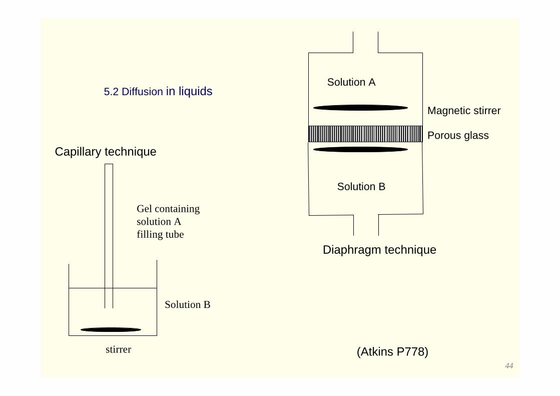
5.2 Diffusion in liquids
Gel containing solution A filling tube
Solution B
stirrer
Capillary technique
(Atkins P778)
Porous glass
Magnetic stirrer
Solution A
Solution B
Diaphragm technique
45
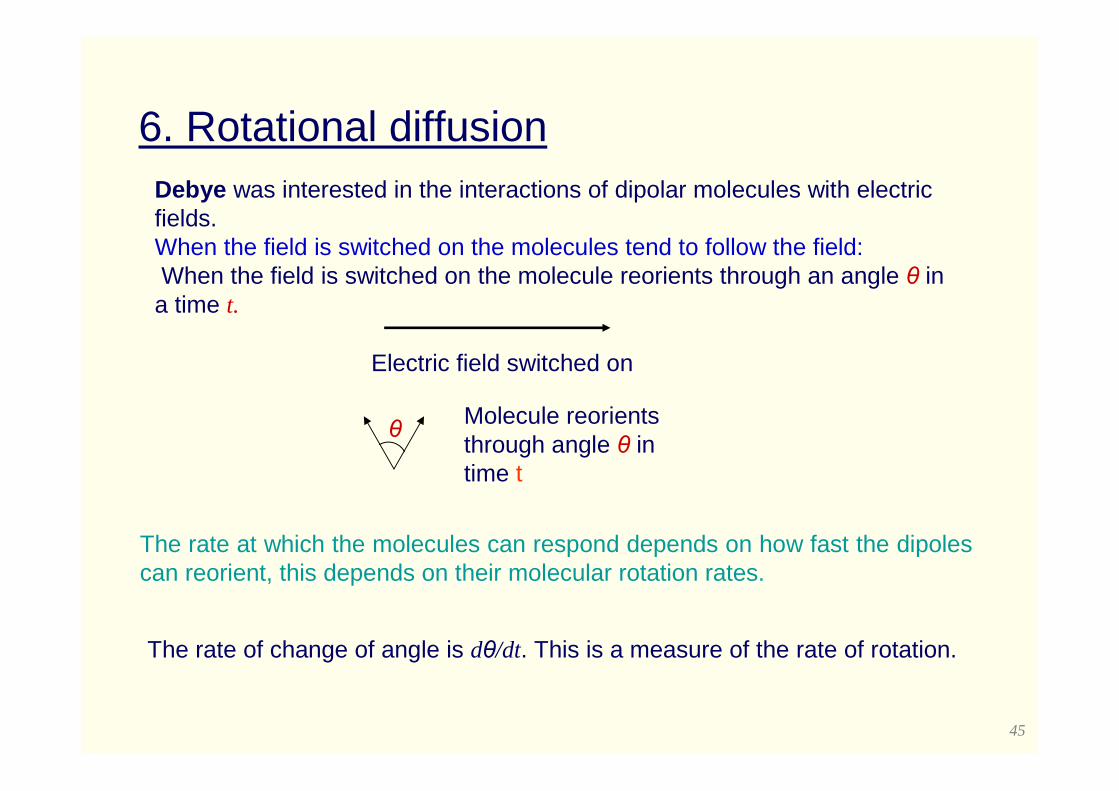
6. Rotational diffusionDebye was interested in the interactions of dipolar molecules with electric fields. When the field is switched on the molecules tend to follow the field:When the field is switched on the molecule reorients through an angle θ in
a time t.
The rate of change of angle is dθ/dt. This is a measure of the rate of rotation.
Electric field switched on
Molecule reorients through angle θ in time t
θ
The rate at which the molecules can respond depends on how fast the dipoles can reorient, this depends on their molecular rotation rates.
46
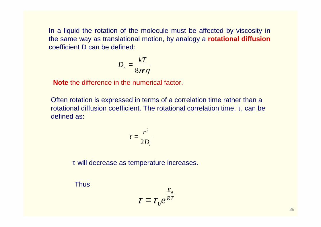
In a liquid the rotation of the molecule must be affected by viscosity in the same way as translational motion, by analogy a rotational diffusioncoefficient D can be defined:
ηπr
kTDr 8
=
Note the difference in the numerical factor.
rD
r
2
2
=τ
Often rotation is expressed in terms of a correlation time rather than a rotational diffusion coefficient. The rotational correlation time, τ, can be defined as:
τ will decrease as temperature increases.
RT
Ea
e0ττ =
Thus
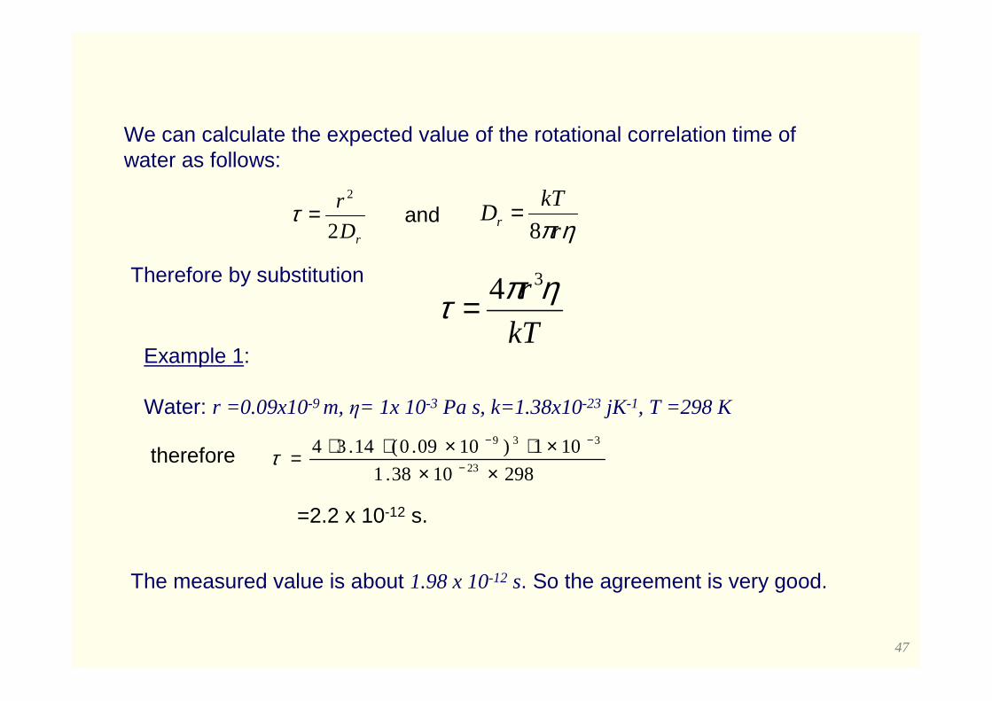
47
We can calculate the expected value of the rotational correlation time of water as follows:
rD
r
2
2
=τηπr
kTDr 8
=and
Therefore by substitution
kT
r ηπτ34=
Example 1:
Water: r =0.09x10⁻⁹ m, η= 1x 10⁻³ Pa s, k=1.38x10⁻²³ jK-1, T =298 K
2981038.1
101)1009.0(14.3423
339
×××⋅×⋅⋅= −
−−
τ
The measured value is about 1.98 x 10⁻¹² s. So the agreement is very good.
=2.2 x 10⁻¹² s.
therefore
48
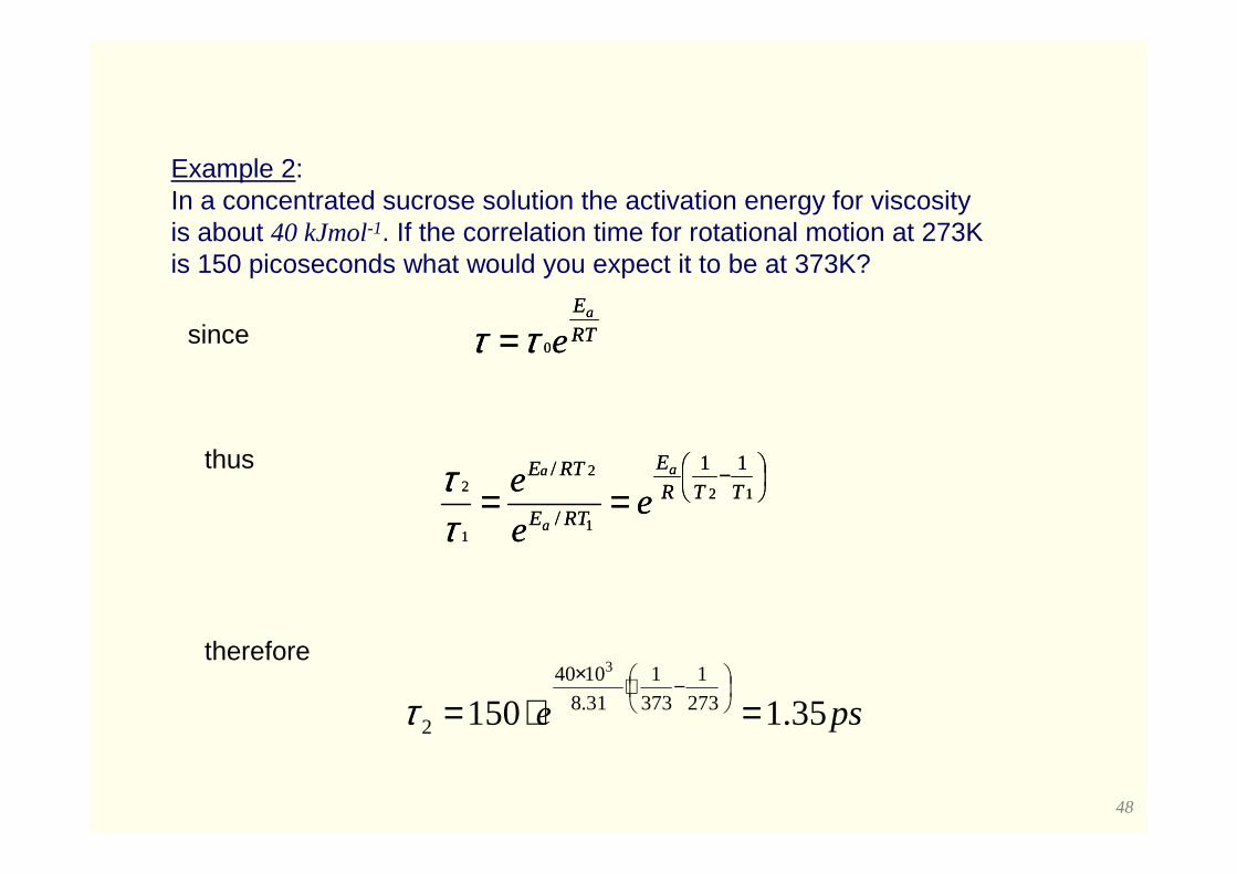
Example 2:In a concentrated sucrose solution the activation energy for viscosity is about 40 kJmol-1. If the correlation time for rotational motion at 273K is 150 picoseconds what would you expect it to be at 373K?
RT
Ea
e0ττ =
−== 12
1
2
1
2
11
/
/TTR
E
RTE
RTE a
a
a
ee
e
ττ
pse 35.1150 273
1
373
1
31.8
1040
2
3
=⋅=
−⋅×
τ
since
thus
therefore
RT
Ea
e0ττ =
−== 12
1
2
1
2
11
/
/TTR
E
RTE
RTE a
a
a
ee
e
ττ
49
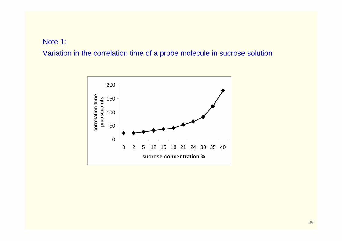
Variation in the correlation time of a probe molecule in sucrose solution
0
50
100
150
200
0 2 5 12 15 18 21 24 30 35 40
sucrose concentration %
corr
elat
ion
time
pico
seco
nds
Note 1:
50
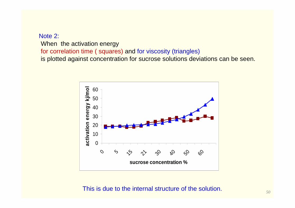
When the activation energy for correlation time ( squares) and for viscosity (triangles)is plotted against concentration for sucrose solutions deviations can be seen.
0
10
20
30
40
50
60
0 5 15 21 30 40 50 60
sucrose concentration %
activ
atio
n en
ergy
kj/m
ol
This is due to the internal structure of the solution.
Note 2:
51
Outline
• 1. Transport properties• 2. Diffusion and viscosity• 2.1 Diffusion process• 2.2 Viscosity• 3. The relationship of diffusion and viscosity– Einstein-
Stokes relationship• 4. The effects of temperature on viscosity and diffusion—
Arrhenius Law• 5. Methods of measurement• 6. Rotational diffusion• 7. using viscosity and diffusion to measure the shapes
and sizes of molecules
52
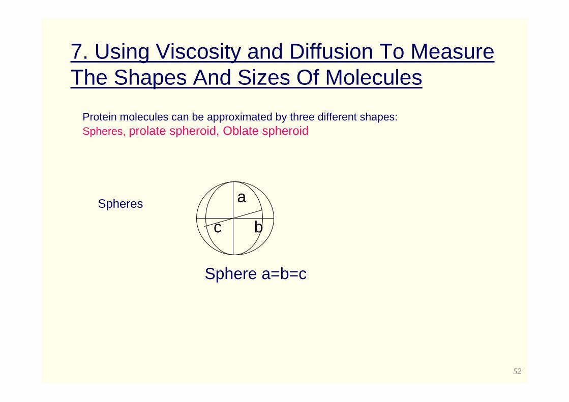
7. Using Viscosity and Diffusion To Measure The Shapes And Sizes Of Molecules
a
bc
Sphere a=b=c
Protein molecules can be approximated by three different shapes:Spheres, prolate spheroid, Oblate spheroid
Spheres
53
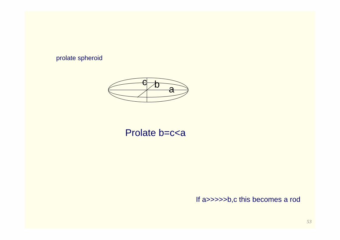
If a>>>>>b,c this becomes a rod
abc
Prolate b=c<a
prolate spheroid
54
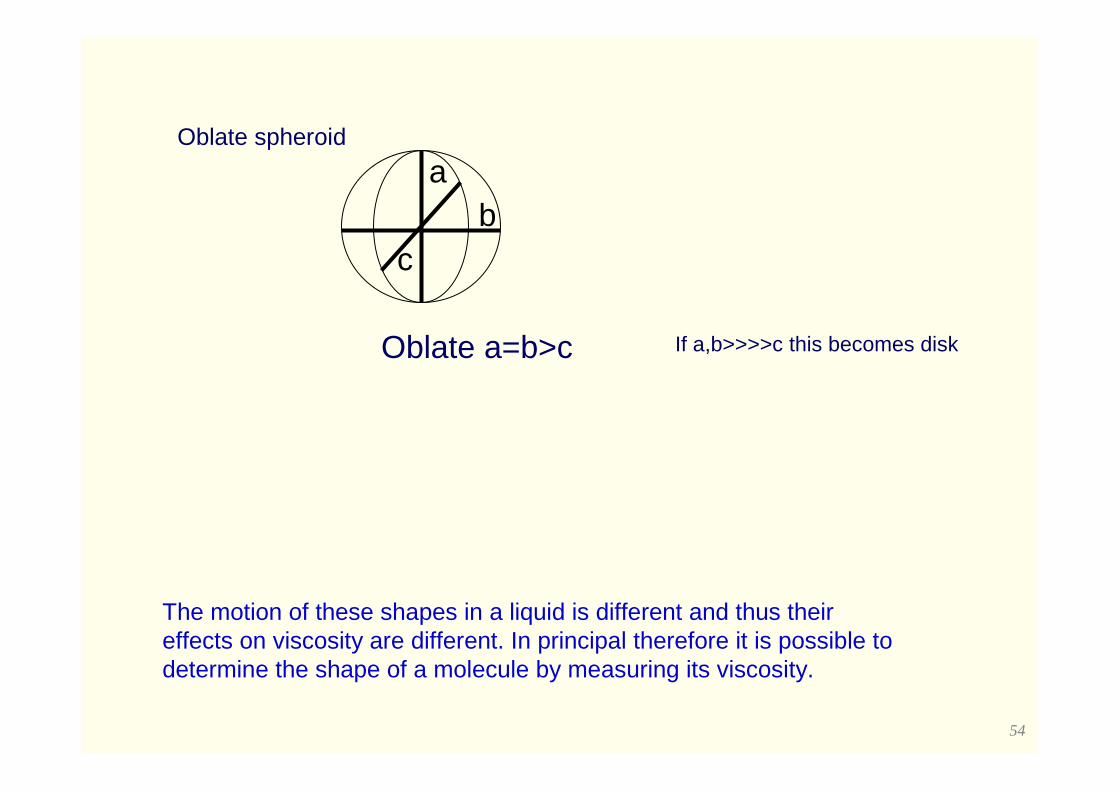
Oblate spheroid
ab
c
Oblate a=b>c If a,b>>>>c this becomes disk
The motion of these shapes in a liquid is different and thus their effects on viscosity are different. In principal therefore it is possible to determine the shape of a molecule by measuring its viscosity.
55
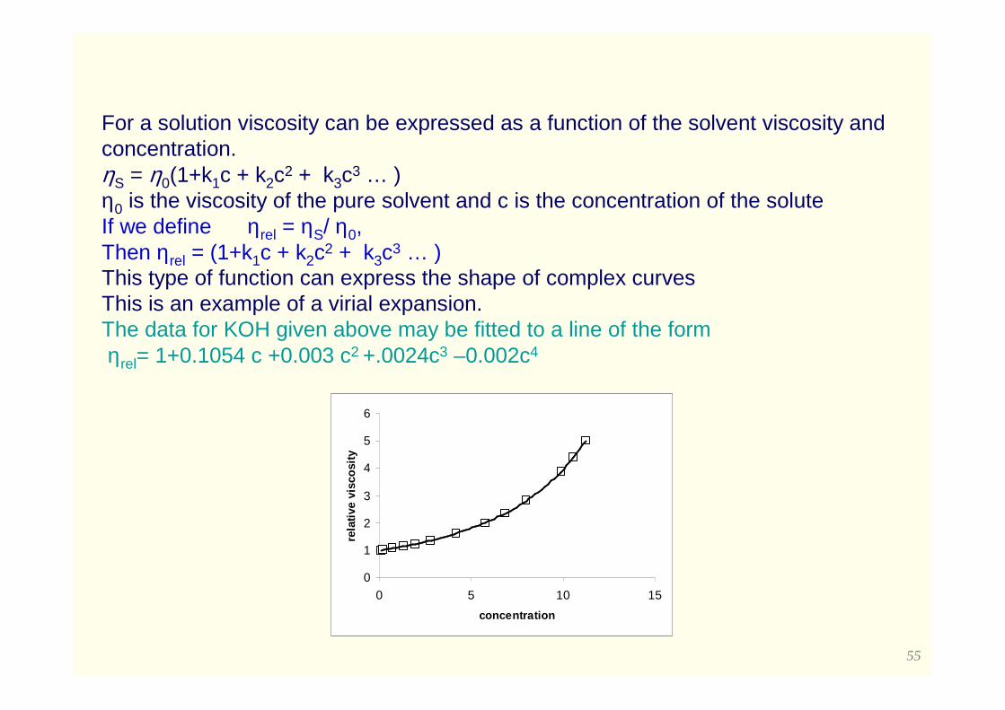
For a solution viscosity can be expressed as a function of the solvent viscosity and concentration.ηS = η0(1+k1c + k2c2 + k3c3 … )η0 is the viscosity of the pure solvent and c is the concentration of the soluteIf we define ηrel = ηS/ η0,Then ηrel = (1+k1c + k2c2 + k3c3 … )This type of function can express the shape of complex curvesThis is an example of a virial expansion.The data for KOH given above may be fitted to a line of the formηrel= 1+0.1054 c +0.003 c2 +.0024c3 –0.002c4
0
1
2
3
4
5
6
0 5 10 15
concentration
rela
tive
visc
osity
56
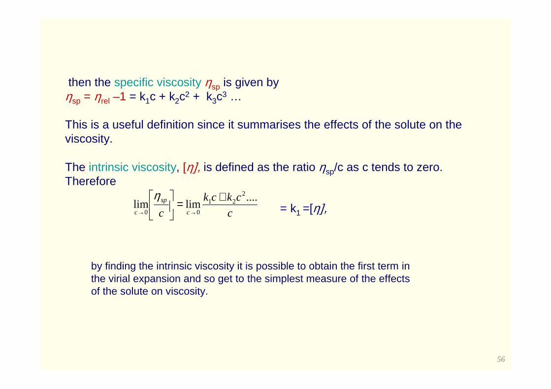
by finding the intrinsic viscosity it is possible to obtain the first term in the virial expansion and so get to the simplest measure of the effects of the solute on viscosity.
then the specific viscosity ηsp is given byηsp = ηrel –1 = k1c + k2c2 + k3c3 …
This is a useful definition since it summarises the effects of the solute on the viscosity.
The intrinsic viscosity, [η], is defined as the ratio ηsp/c as c tends to zero.Therefore
c
ckck
c c
sp
c
....limlim
221
00
+=
→→
η= k1 =[η],
57
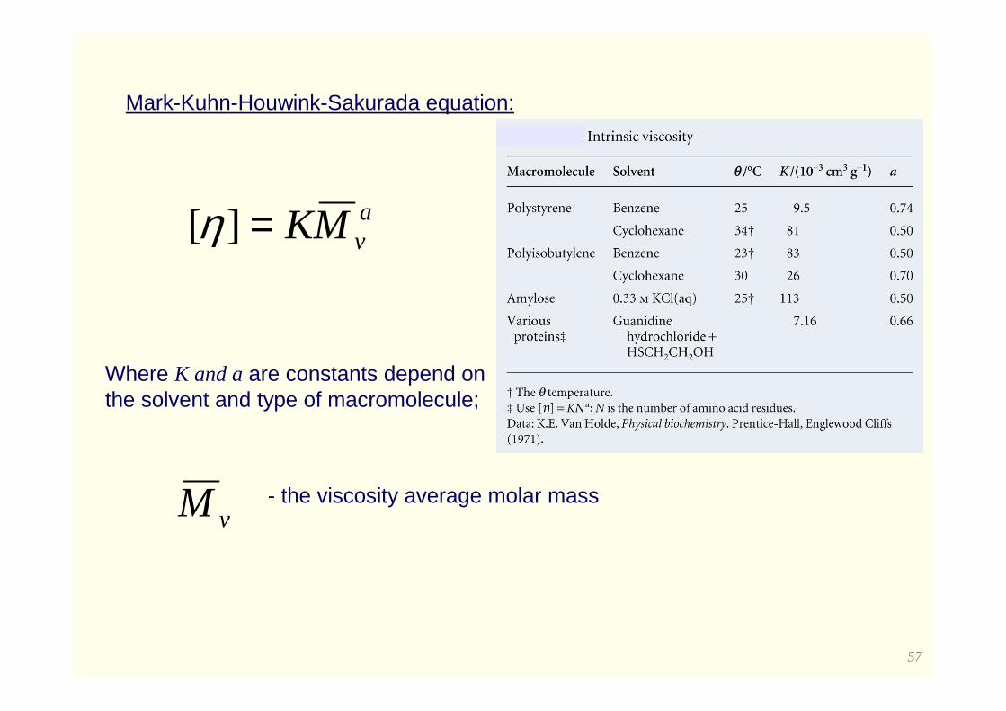
Mark-Kuhn-Houwink-Sakurada equation:
avMK=][η
Where K and a are constants depend on the solvent and type of macromolecule;
vM - the viscosity average molar mass
58
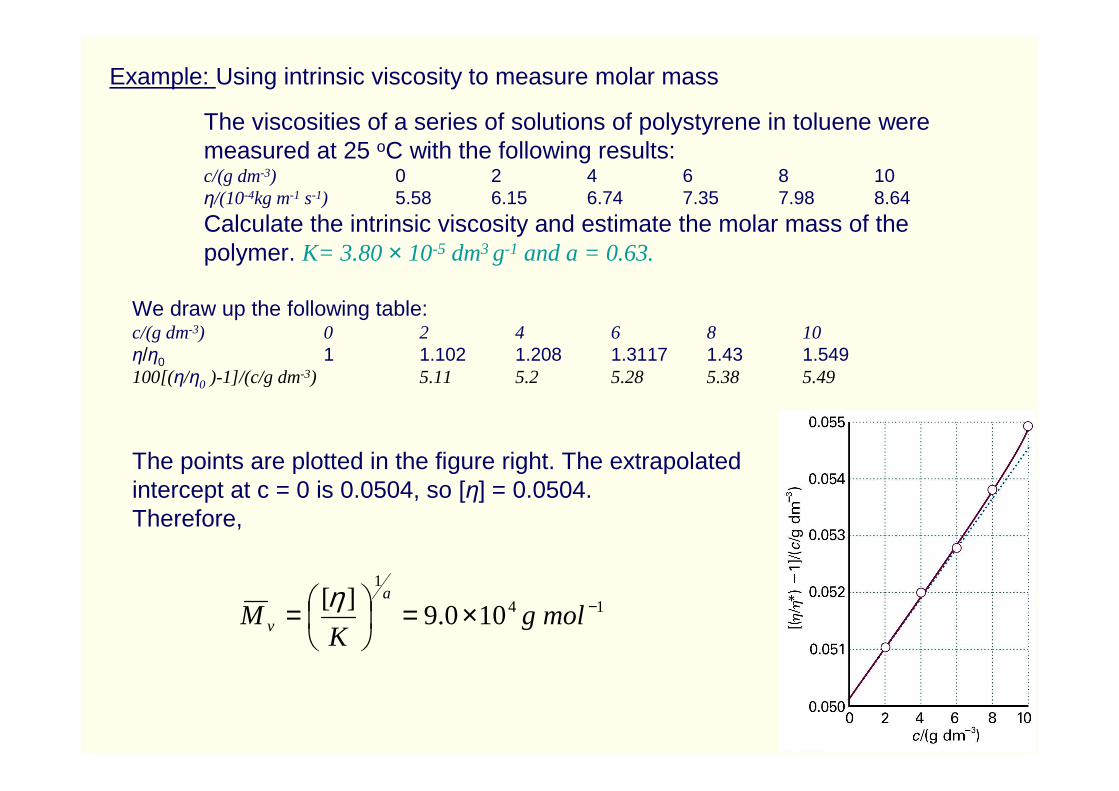
Example: Using intrinsic viscosity to measure molar mass
The viscosities of a series of solutions of polystyrene in toluene were measured at 25 oC with the following results:c/(g dm-3) 0 2 4 6 8 10η/(10-4kg m-1 s-1) 5.58 6.15 6.74 7.35 7.98 8.64
Calculate the intrinsic viscosity and estimate the molar mass of the polymer. K= 3.80 × 10⁻⁵ dm3 g-1 and a = 0.63.
We draw up the following table:c/(g dm-3) 0 2 4 6 8 10η/η0 1 1.102 1.208 1.3117 1.43 1.549100[(η/η0 )-1]/(c/g dm-3) 5.11 5.2 5.28 5.38 5.49
The points are plotted in the figure right. The extrapolated intercept at c = 0 is 0.0504, so [η] = 0.0504.Therefore,
14
1
100.9][ −×=
= molgK
Ma
v
η
59
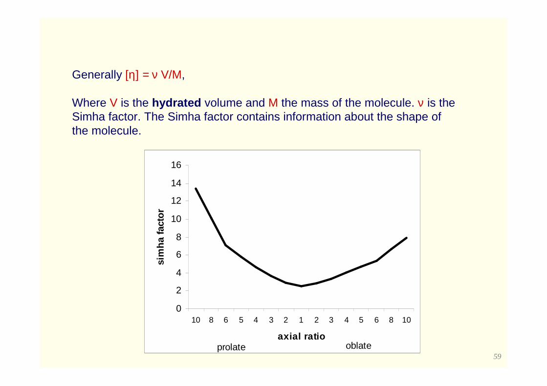
Generally [η] = ν V/M,
Where V is the hydrated volume and M the mass of the molecule. ν is the Simha factor. The Simha factor contains information about the shape of the molecule.
0
2
4
6
8
10
12
14
16
10 8 6 5 4 3 2 1 2 3 4 5 6 8 10
axial ratio
sim
ha fa
ctor
prolate oblate
60
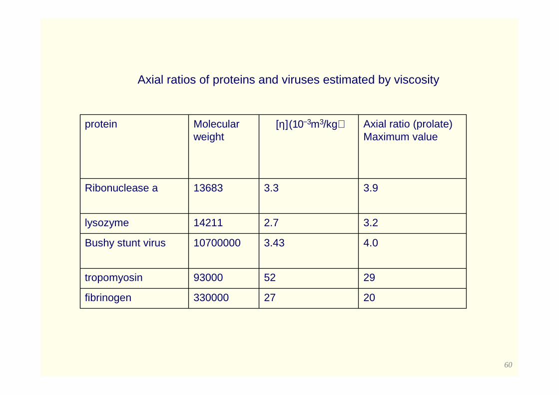
2027330000fibrinogen
295293000tropomyosin
4.03.4310700000Bushy stunt virus
3.22.714211lysozyme
3.93.313683Ribonuclease a
Axial ratio (prolate)Maximum value
[η](10−3m3/kg)Molecular weight
protein
Axial ratios of proteins and viruses estimated by viscosity
61
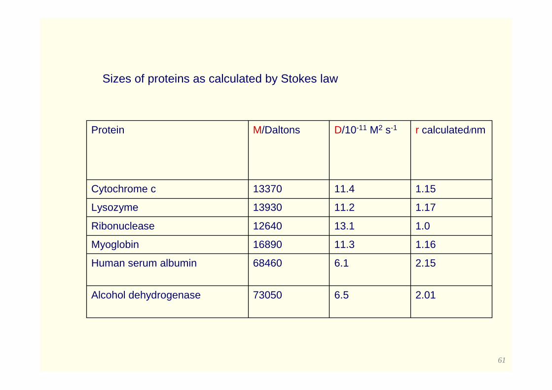
Sizes of proteins as calculated by Stokes law
2.016.573050Alcohol dehydrogenase
2.156.168460Human serum albumin
1.1611.316890Myoglobin
1.013.112640Ribonuclease
1.1711.213930Lysozyme
1.1511.413370Cytochrome c
r calculated/nmD/10-11 M2 s-1M/DaltonsProtein


![Mackiewicz, M. arXiv:1706.05208v4 [cs.CV] 23 Sep 2018 · French, G. g.french@uea.ac.uk Mackiewicz, M. m.mackiewicz@uea.ac.uk Fisher, M. mark.fisher@uea.ac.uk September 25, 2018 Abstract](https://img.pdfslide.us/doc/110x75/5fd4e3c82abb3256c83d0f9c/mackiewicz-m-arxiv170605208v4-cscv-23-sep-2018-french-g-gfrenchueaacuk.jpg)