Cost Engineering

Dr. Nabil I El Sawalhi

Assistant Professor

Construction Management

CE - L9 1

Estimating Methods 2

CE - L9 2

5. Unit quantity

• Unit quantity is used for detail estimating.

• The method sequence is:

• 1. prepare take-off quantities of material.

• 2. Add labor, equipment, and subcontract requirement along with material and quantity for the design.

• The unit quantity model is given by :

• Co =

CE - L9 3

m

i

n

j

HijRijRini1 1

)(

• Where Co= cost for construction cost code or detail, dollars

• ni = quantity for design material i , in dimensional units compatible to design

• Ri = unit cost rate for material i • Rij = unit cost rate for requirement I,j • Hij = unit man or equipment hours for

requirement I,j associated with material ni, • i= material 1,2, … m from take off associated with

construction • j= requirement 1,2, … n to satisfy installation of

material i

CE - L9 4

• Unit cost estimating is given its name because the parameter in the CER is a direct or definitive measure of the units of the item being estimated.

• This is the universal technique for detail estimates based upon take-offs or quantity surveys.

CE - L9 5

• The term line-item refers to the labor hours, labor cost, and material cost for an item are all calculated on a single line of the work sheet

CE - L9 6

• Estimating Process Phase:

• Most commonly applied just prior to construction execution, but it can be used at earlier phases if the detailed input information needed for unit pricing is forced, assumed, or otherwise known.

• Detail engineering and design work is generally greater than 30% complete, and most typically exceeds 60%.

CE - L9 7

CE - L9 8

• Accuracy Range.

• +15/-10% to +5/-5% range before application of contingency (i.e., 90% confidence that actual result will fall within these bounds for the stated scope.

CE - L9 9

Example

• Consider the cross section in Fig 6.3 for section in foundation. Total cost of concrete, material, and labor is required.

• A spread sheet analysis is shown in Table 6.1.

• Different materials are required for this design. But forms and excavation are direct material that are not evident from the foundation wall design. And they are required because the method of doing the work.

CE - L9 10

• The ni is the quantity required for several component for design. It includes excavation, forms, reinforcement, concrete and backfill.

• Observe that 59.3 yd2 of excavation is required for a 4x4 x 100 trench.

• Ri is unit cost of material, Rij are rates for labor and equipment, excavation does not need material (ri=0) but it does need labour and equipments

CE - L9 11

• Forms have a material and labor component, but equipment is not necessary. So n2 H23x R23= 0

• Hij is man-hours per unit of ni quantity.

• For example n1 H12 =59.3x.027 =1.60.

• R12 is the man labor cost which may be for one or more worker including crew work

CE - L9 12

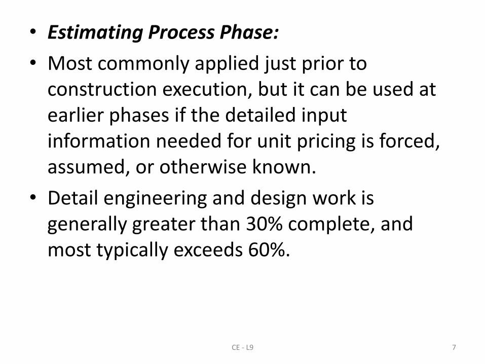
• An ni quantity does not always required material or equipment.

• Concrete material has been identified as requiring contractor labor but the delivery service for concrete is included by the concrete supplier in the cost of concrete.

• The subtotal labor amount of $112 is required for excavation. It is not necessary this matching the equipment requirement as H12 not equal to H13.

• The capital consumption cost or rental cost for the equipment is identified as R13.

CE - L9 13

Example

• For a concrete foundation (excluding excavation): Given: A material quantity parameter and unit cost factors including:

• Quantity = 12 m3 based on take-off from drawings

• Labor factor = 10 hr/m3 from database reference Labor unit rate = $15/labor hour (all-in) from database reference

• Material unit cost = $100/m3 from database reference

CE - L9 14

• Labor $ = 10 hrs/m3 x $15/hr x 12 m3 = $1,800

• Material $ = $100/m3 x 12 m3 = $1,200

• Total direct $ = Labor $ + Material $ = $1,800 + $1,200 = $3,000

• an allowance for indirect costs would then be applied to this figure.

CE - L9 15

7. Factor

• Factor method is also named as ratio or percentage.

• Factor analysis eliminate estimate details.

• It determines the construction estimating summing the product of several quantities.

• C = (Ce+ ∑i fi Ce )(fI+1)

• C = cost of design , dollars

• Ce = cost of major equipment , dollars

CE - L9 16

• fi = factor for estimating major items building, structural steel

• fI = factor for estimating indirect expenses, i e. engineering overheads, number.

• i= 1, 2,…n number.

• The factor method achieves improved accuracy by adopting separate factors for different cost items.

CE - L9 17

• Description

• This method estimates the cost of one item or resource by simply multiplying the known cost of another related item by a given ratio factor.

• The factor is a predetermined, dimensionless ratio of the cost of the unknown resource to the cost of the known one.

CE - L9 18

• The known cost is already derived from one of the major algorithms above, by quotation, or some other means.

• The ratio is determined from analysis of historical data, or obtained from published references, or some other means.

• The method is stochastic if the ratios are derived through regression or other analysis-in that case it is really a simple form of a complex parametric cost model.

CE - L9 19

• It is deterministic if the ratios are definitive relationships such as the case with taxation and labor regulatory burden rates.

• Uses of this method include estimating project indirect costs from direct costs, home office costs from field costs, contingency from estimate total costs, and so on

CE - L9 20

• . It is similar to algorithm adjustment factors in that both use dimensionless factors against a known cost resource, but adjustments are intended to modify a given cost resource and not to derive the cost of another.

CE - L9 21

Example

• For the preliminary cost of Engineering on a chemical process plant.

• Given: • Costs of the base plant and an engineering ratio

factor: • Total field costs (TFC) of a project = $2,500,000 • Engineering ratio factor (Eng$/TFC$) = 0.21 or

21% (from a reference table) • $ Engineering= $2,500,000 x 0.2 1 • = $525,000

CE - L9 22

Cost and Time Estimating Relationships (CERs)

• CERs & Time-estimating Relationshis (TERs) are Mathematical models that estimate cost or time.

• The approach use output design variable (parameters as Ib or yd3) to predict cost. These parameters are called cost drivers.

CE - L9 23

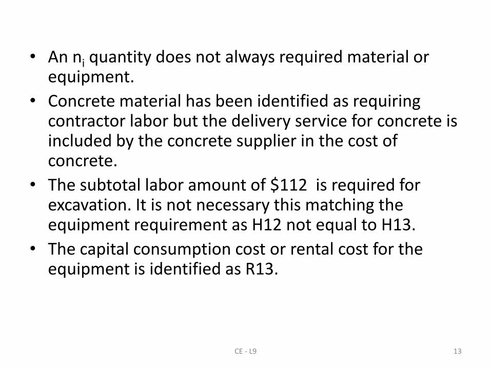
• CERs are developed using the following steps:

• Obtain actual cost

• Interview expert who have knowledge of cost and design.

• Find cost time drivers

• Plot data roughly and understand normality

• Re-plot and conclude regression analysis

• Review for accuracy & communication,

• Publish and distribute the analysis

CE - L9 24

8. Power Law and Sizing

• Power law and sizing CER is used for estimating process and plant equipment.

• This CER models design that vary in size but are similar in type.

• The unknown cost of a 200 gallon kettle can be estimated from data for a 100 gallon kettle provided that they are of similar design. We would not expect the 200-gallon kettle to be twice as costly as the smaller one. The law of economy of scale assures this.

CE - L9 25

• The power –law and sizing CER is given as • C = Cr (Qc/Qr)m

• C = cost for new design size Qc, dollars • Cr= known cost for performance design size Qr, dollars • Q c = design size of equipment expressed in engineering

units • Qr= reference design sized in consistent engineering units. • m = correlating exponent , 0<m<1 • If m= 1, then we have a strictly linear relationship and deny

the law of economy of scale

CE - L9 26

• Table 1 Cost Capacity Exponents for Scaling Costs of Plants Plant or process unit

• Exponent Refrigeration, centrifugal 0.68

• Refrigeration (incl. auxiliaries) 0.85-0.96

• Refrigeration (no auxiliaries) 0.81

• Desalting crude oil 0.60

• LP-gas recovery in refineries 0.70

• Solvent extraction units 0.73

• Polymerization, small plants 0.73

• Polymerization, large plants 0.91

• Solvent dewaxing units 0.82

• Lubricating oil manufacture 0.89

• Clay treating, percolation (incl. regeneration) 0.55

• Clay treating, contact 0.53

• Cracking, thermal (also reforming) 0.51-0.70

• Cracking, thermal, 2-coil 0.79

• Natural gasoline plants 0.73

• The model considers changes in cost due to inflation or deflection and effects independent of size or

• C = Cr (Qc/Qr)m *(Ic/Ir )+ Ci

• Ir= index time-associated with reference equipment, dimensionless number

• Ic = index time-associated with new design dimension less number.

• Ci= cost items independent of design, dollars

CE - L9 28

• Explanation.

• The method consists of four steps:

• 1) obtain the cost and scaling parameter (capacity) of a similar item to the one being estimated,

• 2) normalize that known cost to the proper basis,

• 3) calculate a scale factor-this is a ratio of the scaling parameter values (estimate item over known item) taken

CE - L9 29

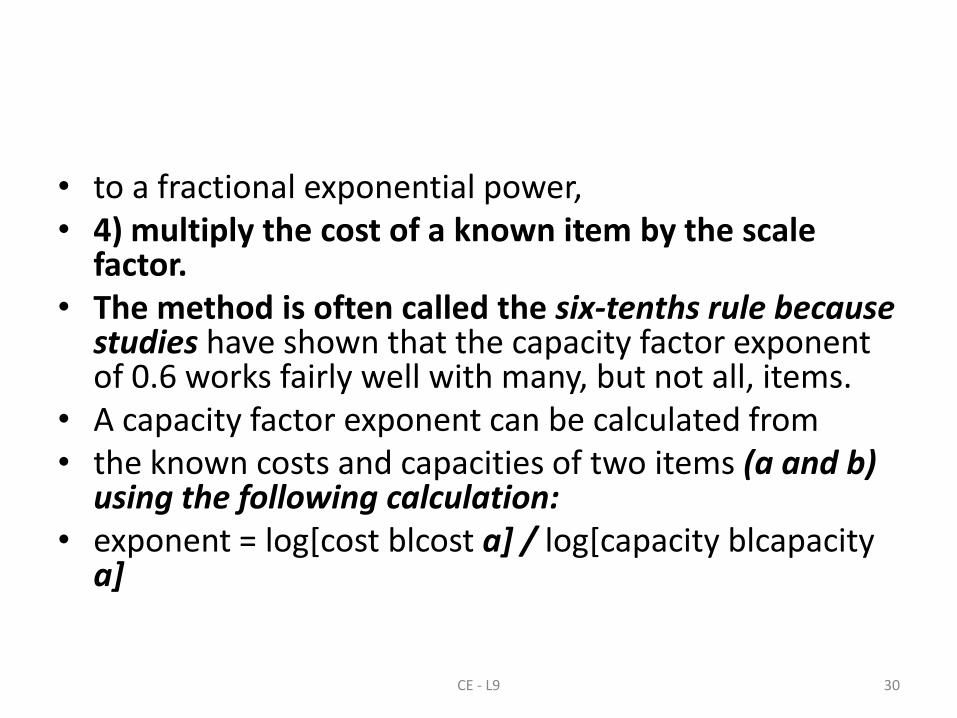
• to a fractional exponential power, • 4) multiply the cost of a known item by the scale

factor. • The method is often called the six-tenths rule because

studies have shown that the capacity factor exponent of 0.6 works fairly well with many, but not all, items.

• A capacity factor exponent can be calculated from • the known costs and capacities of two items (a and b)

using the following calculation: • exponent = log[cost blcost a] / log[capacity blcapacity

a]

CE - L9 30

• Accuracy Range.

• +50/-30% range before application of contingency (i.e., 90% confidence that actual result will fall within these bounds for the stated scope.)

• Type, Source, and References: Stochastic.

• Many general estimating texts include tables of exponent factors.

CE - L9 31

Example 1 • Assume that 6 years ago an 80-kw naturally

aspirated diesel electric set and its plant cost $1,600,000.

• The engineering staff is considering a 120-kw unit of the same general design .

• The value of m= 0.60

CE - L9 32

• The price index for this class of equipment 6 years ago was 187 and now is 194. differing from the previous design is a pre-compressor, which when isolated and estimated separately costs $ 180.000.

• The future cost adjusted for size of the design and for inflation is:

• C = 1600,000 (120/80)0.6(194/187) +180,000

• =$2.3 million

CE - L9 33

Example 2 • For a chemical plant B of type X:

• Given: Cost of comparable plant A parameter, and capacities of plants A and B as follows:

• Cost of Plant A = $10,000,000 (adjusted to current year $)

• Capacity of Plant A = 10,000 unit/day

• Planned capacity of Plant B = 20,000 units/day

CE - L9 34

• e (exponent) = 0.6 (from reference tables for plant of this type)

• Cost Plant B = cost factor x cost of Plant A

• where the cost factor = (capacity of plant 3/capacity of plant A)e

• = (20,000/ 10,000)0.6 x $10,000,000

• = $15,200,000

CE - L9 35

Cost indexes

• 1. Engineering News-Record (ENR) Indexes for building and construction (1913 and 1967 base years).

• 2. Marshall and Swift (M&S) Index of installed equipment (1926 base year).

• 3. Nelson-Farrar Refinery Construction Index (1946 base year).

• 4. Chemical Engineering (CE) Plant Cost Index (base 1957-1959).

• Care must be taken to use the proper index to fit the building, structure, or equipment involved in the specific cost analysis.

Index Number

• Price indices are represented as Incex Number • Number values that indicate relative change but not

absolute values (i.e. one price index value can be compared to another or a base, but the number alone has no meaning).

• Price indices generally select a base year and make that index value equal to 100.

• You then express every other year as a percentage of that base year.

• let's take 2000 as our base year. The value of our index will be 100.)

• 2000: original index value was $2.50; $2.50/$2.50 = 100%, so our new index value is 100

• 2001: original index value was $2.60; $2.60/$2.50 = 104%, so our new index value is 104

• 2002: original index value was $2.70; $2.70/$2.50 = 108%, so our new index value is 108

• 2003: original index value was $2.80; $2.80/$2.50 = 112%, so our new index value is 112

• When an index has been normalized in this manner, the meaning of the number 112, for instance, is that the total cost for the basket of goods is 4% more in 2001, 8% more in 2002 and 12% more in 2003 than in the base year (in this case, year 2000

Cost Indexes

• Cost indexes are dimensionless numerical values

that reflect historical change in costs.

Cost at time A = Index value at time A

Cost at time B Index value at time B

39

Example

Miriam is interested in estimating the annual labor and material costs for a new production facility. She obtained the following data:

• Labor costs:

– Labor cost index value was 124 ten years ago and is 188 today

– Annual labor costs for a similar facility were $575,500 ten years ago

• Material costs

– Material cost index value was at 544 three years ago and is 715 today

– Annual material costs for a similar facility were $2,455,000 three years ago

Annual Cost today = Index value today

Annual cost 10 yrs ago Index value 10 yrs ago

Annual cost today = (188/124) x ($575,500) = $871,800

40

Power-Sizing Model

• Used to estimate the costs of industrial plants and equipment

• It scales up or scales down costs

– Would it cost twice as much to build the same facility with double the

capacity → It is unlikely

Cost of equipment A = Size or capacity of equipment A

Cost of equipment B Size or capacity of equipment B

Where x is the power-sizing exponent

x

If x=1 → linear cost-size relationship

If x>1 → diseconomies of scale

Usually x<1 → economies of scale

41

Example

Miriam needs to estimate the cost of a 2500 ft2 heat exchange system.

• $50,000 for a 1000 ft2 heat exchanger 5 yrs ago

• Power sizing exponent x = 0.55

• Five years ago cost index was 1306; it is 1487 today

Cost of 2500 ft2 equipment = 2500 ft2

Cost of 1000 ft2 equipment 1000 ft2

Cost of the 2500 ft2 equipment (five yrs ago) = 2500 × 50,000 = $82,800

1000

Equipment cost today = $82,800 × 1487 = $94,300

1306

0.55

0.55

42