Downscaling simulations of future global climate with application to

INTERNATIONAL JOURNAL OF CLIMATOLOGY

Int. J. Climatol. 25: 419–436 (2005)

Published online in Wiley InterScience (www.interscience.wiley.com). DOI: 10.1002/joc.1125

DOWNSCALING SIMULATIONS OF FUTURE GLOBAL CLIMATE WITHAPPLICATION TO HYDROLOGIC MODELLING

ERIC P. SALATHE JR*Center for Science in the Earth System, Joint Institute for the Study of the Atmosphere and Ocean, University of Washington, Seattle,

WA, USA

Received 22 September 2003Revised 6 August 2004

Accepted 22 August 2004

ABSTRACT

This study approaches the problem of downscaling global climate model simulations with an emphasis on validating andselecting global models. The downscaling method makes minimal, physically based corrections to the global simulationwhile preserving much of the statistics of interannual variability in the climate model. Differences among the downscaledresults for simulations of present-day climate form a basis for model evaluation. The downscaled results are used tosimulate streamflow in the Yakima River, a mountainous basin in Washington, USA, to illustrate how model differencesaffect streamflow simulations. The downscaling is applied to the output of three models (ECHAM4, HADCM3, andNCAR-PCM) for simulations of historic conditions (1900–2000) and two future emissions scenarios (A2 and B2 for2000–2100) from the IPCC assessment. The ECHAM4 simulation closely reproduces the observed statistics of temperatureand precipitation for the 42 year period 1949–90. Streamflow computed from this climate simulation likewise producessimilar statistics to streamflow computed from the observed data.

Downscaled climate-change scenarios from these models are examined in light of the differences in the present-daysimulations. Streamflows simulated from the ECHAM4 results show the greatest sensitivity to climate change, withthe peak in summertime flow occurring 2 months earlier by the end of the 21st century. Copyright 2005 RoyalMeteorological Society.

KEY WORDS: Pacific Northwest; statistical downscaling; hydrology; hydrologic modelling; precipitation; streamflow; climate change

1. INTRODUCTION

Studies of the regional impacts of climate change must confront the problem of choosing climate-changescenarios. The task of downscaling global climate model (GCM) simulations is often so demanding thatonly a limited selection of models and greenhouse-gas emission scenarios may be considered. However, itis preferable to consider a range of scenarios in climate impacts studies (e.g. see Houghton et al. (2001:741). The use of several models and emissions scenarios better reflects the uncertainty in the range ofpossible future climate change. Furthermore, model performance varies for different regions or the processunder consideration. Thus, impacts studies must consider several model simulations and must evaluate modelperformance, using simulations of present-day conditions.

The models and emissions scenarios included in the recent Intergovernmental Panel on Climate Change(IPCC) report (Houghton et al., 2001) form a standardized collection of scenarios appropriate to many studies.GCM model simulations for these scenarios are available via the Internet (http://ipcc-ddc.cru.uea.ac.uk/) forsix models and up to seven emissions scenarios each. A selection of three models from this archive is presentedin this paper. Simulations using historic forcing for 1900–90 and two future emissions scenarios, A2 and B2,for 1990–2100 will be considered.

* Correspondence to: Eric P. Salathe Jr, Climate Impacts Group, University of Washington, Box 354235, Seattle, WA 98195, USA;e-mail: [email protected]

Copyright 2005 Royal Meteorological Society

420 E. P. SALATHE JR

A simple empirical method (Salathe, 2003; Widmann et al., 2003) is applied to downscale the globalsimulations to 0.125° resolution. The downscaling method is implemented using readily available data and isfast enough to downscale a large collection of scenarios for long time periods. The downscaled results are thenapplied to simulate streamflow in the Yakima River, a mesoscale river basin in central Washington, USA. Theeffect of climate change on hydrologic processes is an important factor in the impacts of climate on manyregions worldwide. Thus, the suitability of the downscaled data for hydrologic modelling is an importanttest of the global model simulation and the downscaling. The examples presented will illustrate how thedownscaled results may be evaluated as part of model selection for an impacts study. Other studies haveexamined the streamflow response of this and similar regions to climate change (Hamlet and Lettenmaier,1999; Hay et al., 2000, 2002). This paper will focus on the quality of the global simulations forced by historicclimate conditions as a means to verify the climate-change simulations. Since the downscaling method is quitesimple and only weakly constrains the global simulation, the statistics of the global model’s variability areessentially preserved by the downscaling.

Downscaling methods are reviewed in Wilby et al. (1998) and Giorgi et al. (2001). The downscalingmethods presented here are statistical methods and are based on empirical relationships between large-scaleand mesoscale climate variables. Statistical downscaling may be contrasted to downscaling via a physicalmesoscale model nested within the global model. Many statistical methods for precipitation downscaling arebased on a large-scale predictor other than precipitation. A circulation parameter is the most common predictor,and often atmospheric moisture is considered as well (see Wilby and Wigley (2000) for an overview of variouspredictors for downscaling precipitation). The method presented here, however, is based upon precipitationas the large-scale predictor, as motivated by Widmann and Bretherton (2000).

All data used to perform the downscaling are freely available over the Internet. The climate modelsimulations are available from the IPCC Data Distribution Centre Website (http://ipcc-ddc.cru.uea.ac.uk/).High-resolution gridded temperature and precipitation used to fit the downscaling method are available forNorth America from the Website of the Surface Water Modelling group at the University of Washington(http://www.hydro.washington.edu/Lettenmaier/gridded data).

2. DATA AND METHODS

2.1. Downscaling method

Typical GCMs are run with a grid resolution of approximately 2.5° (∼300 km), whereas regional climateimpacts studies often require resolutions of 0.125° (∼15 km) or finer. Furthermore, publicly available archivesare typically monthly mean fields. Thus, regionalizing the simulations requires spatial downscaling andtemporal disaggregation. Downscaling both accounts for subgrid-scale processes not included in the globalsimulation and disaggregates the grid cells to the required resolution. For this study, we consider onlytemperature and precipitation, which are the essential parameters for simulating the effects of climate changeon hydrology. For both parameters, the large-scale simulated values from the global models will be thepredictors for the downscaling. To downscale precipitation, the method developed by Widmann et al. (2003),referred to as the ‘local scaling’, will be used. A similar, local, method will be used for temperature. Thedownscaling applies to monthly means.

Temporal disaggregation is performed following a modified version of the method in Wood et al. (2002).Although the spatial pattern of precipitation is not well represented in global models, the temporal variabilityat a fixed location may be simulated realistically depending upon the meteorological mechanism producingprecipitation. In the Pacific Northwest, the large-scale precipitation simulated by the atmospheric model usedin the National Centers for Environmental Prediction (NCAR)–National Center for Atmospheric Research(NCEP) reanalyses is well correlated in time to the station observations at various locations (Widmann andBretherton, 2000). At any location and season, the bias between the large-scale simulated precipitation andobserved precipitation is the same from year to year. Precipitation events for this region are produced by large-scale weather systems that are well resolved by the global model, and these systems control the precipitation

Copyright 2005 Royal Meteorological Society Int. J. Climatol. 25: 419–436 (2005)

DOWNSCALING APPLICATION TO HYDROLOGIC MODELLING 421

variability on the monthly time scale. Thus, the local scaling method performs as well as more sophisticateddownscaling methods for this region when applied to the NCEP reanalyses.

Although one cannot validate the downscaling of a free-running GCM against observations as withreanalyses, the GCMs presented here are of similar sophistication to the NCEP reanalysis model and wellrepresent mid-latitude storm systems. We assume, therefore, that the monthly variability and long-term trendin precipitation is likewise well represented by the GCM. Thus, the downscaling method takes the monthlytemporal variability from the simulation and uses empirical data to impose the correct spatial structure. In thisway, the downscaling method responds well to the processes driving climate change in simulated precipitationand surface temperature.

In previous work (Salathe, 2003; Widmann et al., 2003), a 50 km gridded precipitation data set (Widmannand Bretherton, 2000) was used as the observed field for fitting parameters in the precipitation downscaling.In this paper, downscaling will be to a finer-resolution grid using a 0.125° data set of daily precipitation,maximum temperature, and minimum temperature (Maurer et al., 2002). The data are derived by combiningdaily station observations with the long-term monthly climatology from the parameter-elevation regressionson independent slopes model (PRISM; Daly et al., 1994) to produced gridded daily fields. This data set spansthe period 1 January 1949 to 31 July 2000 and is available from the Surface Water Modelling group at theUniversity of Washington from their Website at http://www.hydro.washington.edu/Lettenmaier/gridded data/.The methods described here would be equally applicable to station data as to gridded data. In that case, theclimate simulations would be downscaled directly to the station locations

The empirical parameters in the downscaling methods are fit to these observed fields independently foreach model using the model climatology for present-day conditions. Tuning the method specifically for themodel to be downscaled is an essential feature of this downscaling method. In some downscaling methods, theglobal simulation used for tuning must duplicate the actual historic weather sequence, which requires using areanalysis-type run rather than a free-running control simulation for tuning. Here, free-running is used to meanthe model is not constrained in any way by proscribing the lower boundary condition or by assimilating stationobservations; only the atmospheric composition and solar output are specified. Coupled atmosphere–oceanclimate model simulations are generally performed as a free-running simulation. If the model to be downscaledis not used to tune the method, then the biases inherent to the model cannot be removed, which is one ofthe essential tasks of downscaling. If the downscaling method is tuned to reanalyses and then applied to afree-running simulation of a climate model for present-day conditions, then the results are a poor match tothe observed climatology (e.g. see Hay et al. (2000)). By tuning the downscaling method to the long-termmean precipitation and surface temperature the method may be tuned to a relatively short control run of eachclimate model that is to be downscaled. Although this approach is more cumbersome than using a single setof empirical parameters for all models, once the method has been fit to a model then any number of climatescenarios or ensemble members simulated with that model may be downscaled using those parameters.

The control runs used to fit each model are simulations forced by historic variations in greenhouse gases,solar output, and atmospheric aerosol loading; this control run will be referred to as the ‘historic’ run of themodel. For each of the models presented here, results for a historic run were provided in the IPCC archive.For consistency, only the years where the historic simulation and observed data overlap are used to derivethe scaling factors, typically 1949 to 1990.

2.1.1. Precipitation. In Widmann et al. (2003), a precipitation downscaling method using large-scaleprecipitation as predictor is developed and referred to as ‘local’ scaling. The local scaling method simplymultiplies the large-scale simulated precipitation at each local gridpoint by a seasonal scale factor. The scalingfactor is derived during a fitting period in order to remove the long-term bias between the large-scale simulatedprecipitation and the observed precipitation at that gridpoint. Thus, if Pmod(x, t) is the simulated large-scalemonthly mean precipitation for the gridpoint containing a location x and at time t in season ‘sea’, then thedownscaled monthly mean precipitation is

Pds(x, t) = Pmod(x, t)〈Pobs〉sea

〈Pmod〉sea(1)



where 〈. . .〉sea is the seasonal mean taken over the fitting period (i.e. the overlap of the observed data set and thehistoric run). The fitting is performed independently for each 3 month season, December–January–February(DJF), March–April–May (MAM), June–July–August (JJA), September–October–November (SON).

In previous work, this method was evaluated by comparing downscaled results from the NCAR–NCEPreanalyses with observations (Widmann et al., 2003) and by using these results to drive a hydrologic modelof the Yakima River basin (Salathe, 2003). A more sophisticated nonlocal scaling, referred to as ‘dynamicalscaling’, was also presented in Widmann et al. (2003), which exhibited much better results for the driestportions of the rain shadow in eastern Washington. In hydrologic simulations for the Yakima River, driven bydownscaled NCAR–NCEP reanalyses, however, the nonlocal scaling method showed no advantage (Salathe,2003). These results suggest that the local scaling method is quite suitable for a range of regional climatestudies.

2.1.2. Surface temperature. Surface air temperature is downscaled in a similar way to precipitation. Fortemperature the adjustment is additive; thus, the downscaled monthly mean surface temperature is given by

Tds(x, t) = Tmod(x, t) + [〈Tobs〉sea − 〈Tmod〉sea] (2)

where 〈. . .〉sea is the seasonal mean taken over the fitting period. Essentially, this correction assumes that thelocal temperature is found from the large-scale temperature simply by removing a seasonal bias in the mean.This addition can be thought of as a lapse-rate correction due to the elevation difference of the local gridpointrelative to the GCM grid. Thus, if the lapse rate is strongly affected by climate change, then this assumptionwould break down.

The downscaling is performed on surface air temperature, i.e. at 2 m. In the observed data set, the minimumand maximum daily temperatures are averaged to produce mean surface temperature.

2.1.3. Temporal disaggregation. The monthly mean precipitation and temperature fields archived fromthe climate simulations are downscaled to high-resolution fields by the above methods. To drive modelsthat require daily time resolution, such as hydrologic or ecologic models, monthly means must then bedisaggregated into daily sequences. Although the daily global simulation could be used when available,as was done with the NCAR–NCEP reanalyses in Salathe (2003), it is not clear that using daily weathersequences from a free-running GCM is warranted, even when such data are readily available. The ability ofthe GCM to simulate changes in the frequency and magnitude of extreme weather events is much less certainthan the ability to simulate the longer term trends captured in monthly means. Assuming the daily weatherpatterns remain essentially the same in the future, we can disaggregate the simulated monthly means usinghistoric weather sequences

The method used here is an extension of that used by Wood et al. (2002), where the daily weather sequenceis obtained by selecting a month from the observed record. The daily variability from that month is imposed onall gridpoints while preserving the downscaled monthly mean. However, two months with a similar monthlytotal precipitation could yield significantly different streamflows depending upon whether the precipitationfalls in a few heavy events or occurs as drizzle throughout the month. Large-scale features from the simulationshould help choose a better analogue from the past than a random selection. In this paper, we use a methodwhere the analogue is selected by choosing a month in the season to be downscaled with the closest matchbetween the observed and downscaled monthly mean precipitation pattern. Presumably, a particular regionalprecipitation pattern would occur under specific meteorological conditions and the daily weather sequencewill be similar for months with similar regional patterns. Using a precipitation analogue also helps avoidproblems where the selected month has a dramatically different monthly mean than the downscaled month atsome grid points. The same analogue month is used to disaggregate both temperature and precipitation.

Once an analogue month is selected, the observed daily values at each gridpoint are adjusted to thedownscaled monthly mean to produce the disaggregated downscaled time series. For precipitation, theadjustment is multiplicative. The daily values from the analogue month are divided by the analogue-monthmean and multiplied by the downscaled-month mean to produce daily downscaled precipitation. For surface



temperature, the disaggregation also yields daily minimum (Tmin) and maximum (Tmax) temperatures. Theobserved sequence of Tmin and Tmax for the selected month are each shifted by a constant factor τ such thatthe shifted daily mean temperature

(Tmin + Tmax) × 0.5 + τ (3)

averaged over the month, equals the downscaled monthly mean surface temperature. Thus, the diurnal rangeis taken from the analogue month and is not subject to climate change.

2.2. Global climate simulations and emissions scenarios

The above downscaling methods will be applied to three climate models in the IPCC archive: (1) The MaxPlanck Institute fur Meteorologie ECHAM4/OPYC3 (hereafter ECHAM4) (Roeckner et al., 1999; Stendelet al., 2000); (2) The Hadley Centre for Climate Prediction and Research HADCM3 (Mitchell et al., 1998;Gregory and Lowe, 2000; Johns et al., 2001); (3) The Department of Energy (DOE)–NCAR parallel climatemodel (hereafter NCAR-PCM; Washington et al., 2000; Meehl et al., 2001). Three simulations from eachmodel will be downscaled: a simulation forced by historic conditions (HST), and two forced by futureemissions scenarios, the SRES A2 and B2.

The HST simulations all include the historic variation of anthropogenic greenhouse gases, anthropogenicand natural aerosol, and solar output. The SRES A2 and B2 scenarios describe two different projectionsof greenhouse-gas emissions and aerosol concentrations (Nakicenovic et al., 2000). These scenarios producesimilar total radiative forcing up to the 2040s; in the later half of the century, the A2 scenario producesconsiderably more radiative forcing than B2. Slightly different time periods are available for each model, assummarized in Table I.

The HST simulation from each model is also used to tune the downscaling method applied to thatmodel, but only the period 1949–90 is used (1960–90 for NCAR-PCM). Thus, part of the downscaledHST simulation overlaps with the data period used to fit the downscaling method. This would tend to producebetter performance of the downscaling method during this period; however, the method has been evaluatedin a more rigorous manner elsewhere (Salathe, 2003; Widmann et al., 2003).

2.3. Hydrologic model

To evaluate the applicability of the downscaled results, streamflow for the Yakima River is simulated forthe period 1900–2100 for each model and scenario using the variable infiltration capacity (VIC) hydrologymodel (Liang et al., 1994) implemented at 0.125° resolution (Hamlet and Lettenmaier, 1999). The 0.125° VICmodel is very similar to the model implemented at 0.25° described by Matheussen et al. (2000). Simulatedgrid-cell runoff and baseflow are then processed with a river routing model (Lohmann et al., 1996, 1998)

Table I. Models and scenarios to which downscaling isapplied

Model Scenario Years

ECHAM4 HST 1900–90A2 1990–2100B2 1990–2100

HADCM3 HST 1900–90A2 1990–2099B2 1990–2099

NCAR-PCM HST 1960–99A2 1990–2099B2 2000–99



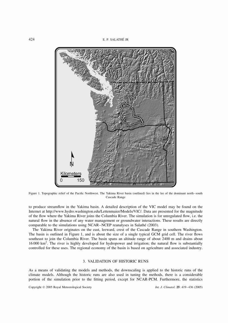
Figure 1. Topographic relief of the Pacific Northwest. The Yakima River basin (outlined) lies in the lee of the dominant north–southCascade Range

to produce streamflow in the Yakima basin. A detailed description of the VIC model may be found on theInternet at http://www.hydro.washington.edu/Lettenmaier/Models/VIC/. Data are presented for the magnitudeof the flow where the Yakima River joins the Columbia River. The simulation is for unregulated flow, i.e. thenatural flow in the absence of any water management or groundwater interactions. These results are directlycomparable to the simulations using NCAR–NCEP reanalyses in Salathe (2003).

The Yakima River originates on the east, leeward, crest of the Cascade Range in southern Washington.The basin is outlined in Figure 1, and is about the size of a single typical GCM grid cell. The river flowssoutheast to join the Columbia River. The basin spans an altitude range of about 2400 m and drains about16 000 km2. The river is highly developed for hydropower and irrigation; the natural flow is substantiallycontrolled for these uses. The regional economy of the basin is based on agriculture and associated industry.

3. VALIDATION OF HISTORIC RUNS

As a means of validating the models and methods, the downscaling is applied to the historic runs of theclimate models. Although the historic runs are also used in tuning the methods, there is a considerableportion of the simulation prior to the fitting period, except for NCAR-PCM. Furthermore, the statistics



presented here are not forced to match the observations by the downscaling. In Section 3.1 the basin-meantemperature and precipitation time series from the climate model simulations will be compared with the timeseries from the gridded observations. Section 3.2 compares streamflows simulated from the climate modelresults against streamflows simulated from gridded observations. The comparisons will examine whetherthe climate models simulate realistic interannual variability for these parameters once the local biases inprecipitation and temperature are removed. Since the models are free running, only those climate variationsattributable to the slow changes in greenhouse gases, aerosols, and solar output can be expected to matchobservations for the simulated date. Interannual variability is entirely internal to the model dynamics andcannot match observations for the coincident date. Ideally, a model will simulate realistic statistical propertiesof the interannual variability, which is essential to the climate impacts of the Pacific Northwest. Somedownscaling methods, such as the bias correction method (Wood et al., 2002), force the probability distributionof temperature and precipitation for the historic simulation to match the observed distributions. The methodused here does not attempt to correct the statistics of the simulated parameters, but rather preserves these asa basis for model evaluation.

3.1. Basin-mean precipitation and temperature

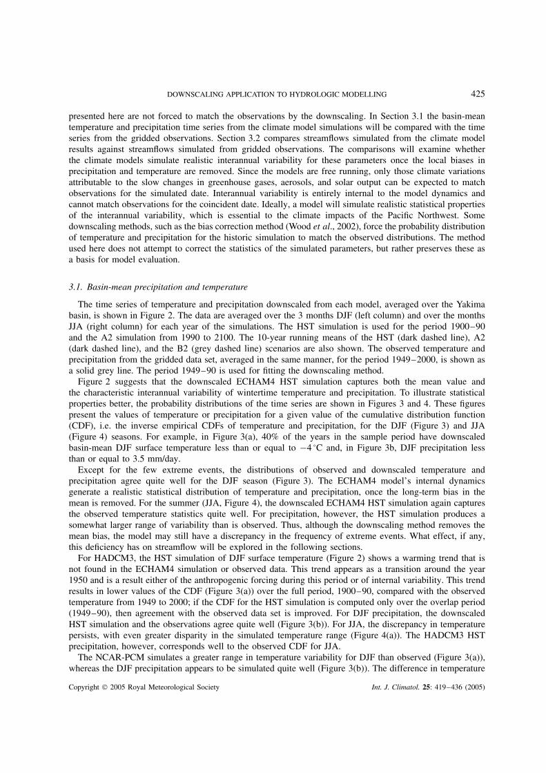
The time series of temperature and precipitation downscaled from each model, averaged over the Yakimabasin, is shown in Figure 2. The data are averaged over the 3 months DJF (left column) and over the monthsJJA (right column) for each year of the simulations. The HST simulation is used for the period 1900–90and the A2 simulation from 1990 to 2100. The 10-year running means of the HST (dark dashed line), A2(dark dashed line), and the B2 (grey dashed line) scenarios are also shown. The observed temperature andprecipitation from the gridded data set, averaged in the same manner, for the period 1949–2000, is shown asa solid grey line. The period 1949–90 is used for fitting the downscaling method.

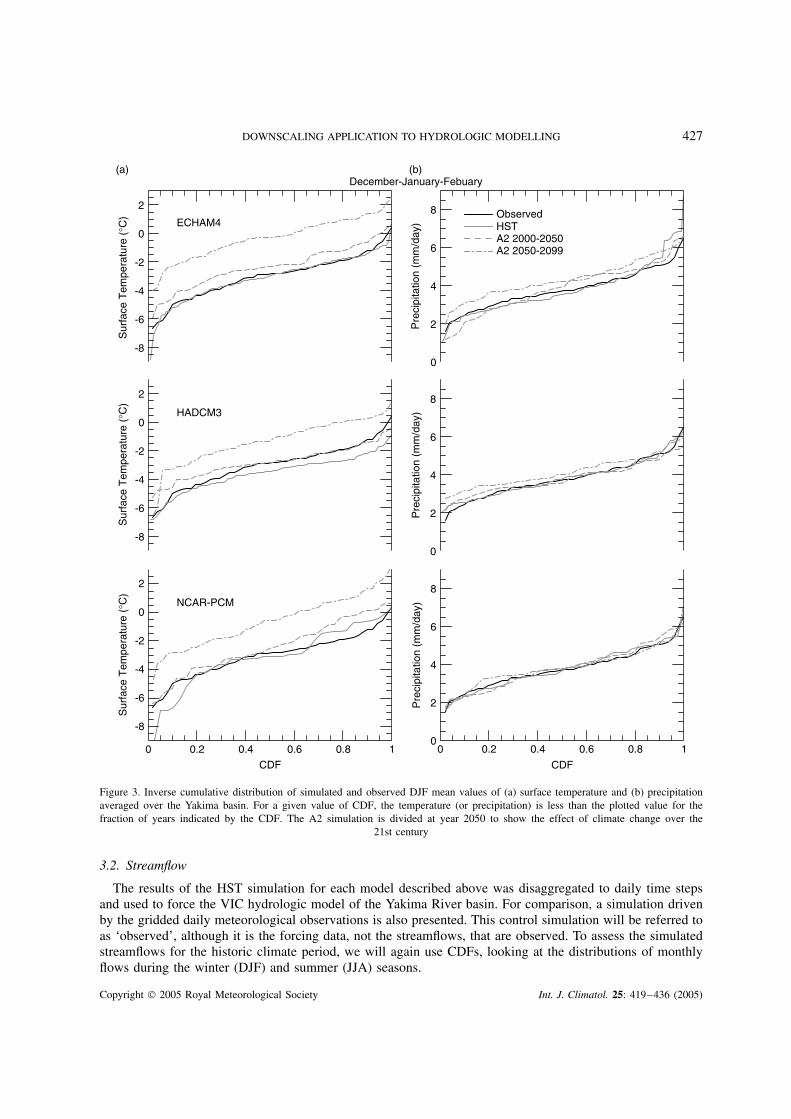
Figure 2 suggests that the downscaled ECHAM4 HST simulation captures both the mean value andthe characteristic interannual variability of wintertime temperature and precipitation. To illustrate statisticalproperties better, the probability distributions of the time series are shown in Figures 3 and 4. These figurespresent the values of temperature or precipitation for a given value of the cumulative distribution function(CDF), i.e. the inverse empirical CDFs of temperature and precipitation, for the DJF (Figure 3) and JJA(Figure 4) seasons. For example, in Figure 3(a), 40% of the years in the sample period have downscaledbasin-mean DJF surface temperature less than or equal to −4 °C and, in Figure 3b, DJF precipitation lessthan or equal to 3.5 mm/day.

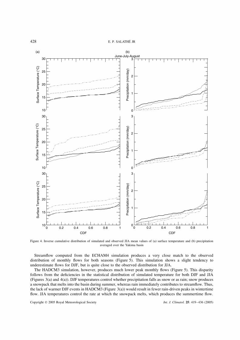
Except for the few extreme events, the distributions of observed and downscaled temperature andprecipitation agree quite well for the DJF season (Figure 3). The ECHAM4 model’s internal dynamicsgenerate a realistic statistical distribution of temperature and precipitation, once the long-term bias in themean is removed. For the summer (JJA, Figure 4), the downscaled ECHAM4 HST simulation again capturesthe observed temperature statistics quite well. For precipitation, however, the HST simulation produces asomewhat larger range of variability than is observed. Thus, although the downscaling method removes themean bias, the model may still have a discrepancy in the frequency of extreme events. What effect, if any,this deficiency has on streamflow will be explored in the following sections.

For HADCM3, the HST simulation of DJF surface temperature (Figure 2) shows a warming trend that isnot found in the ECHAM4 simulation or observed data. This trend appears as a transition around the year1950 and is a result either of the anthropogenic forcing during this period or of internal variability. This trendresults in lower values of the CDF (Figure 3(a)) over the full period, 1900–90, compared with the observedtemperature from 1949 to 2000; if the CDF for the HST simulation is computed only over the overlap period(1949–90), then agreement with the observed data set is improved. For DJF precipitation, the downscaledHST simulation and the observations agree quite well (Figure 3(b)). For JJA, the discrepancy in temperaturepersists, with even greater disparity in the simulated temperature range (Figure 4(a)). The HADCM3 HSTprecipitation, however, corresponds well to the observed CDF for JJA.

The NCAR-PCM simulates a greater range in temperature variability for DJF than observed (Figure 3(a)),whereas the DJF precipitation appears to be simulated quite well (Figure 3(b)). The difference in temperature



-8

-6

-4

-2

0

2

Jan-1900 Jan-1950 Jan-2000 Jan-2050 Jan-21000

2

4

6

8

10

Pre

cipi

tatio

n (m

m/d

ay)

ECHAM4

HADCM3

NCAR-PCM

Sur

face

Tem

pera

ture

(°C

)

10

15

20

25

30


1

2

3

-8

-6

-4

-2

0

2


2

4

6

8

10

Pre

cipi

tatio

n (m

m/d

ay)

Sur

face

Tem

pera

ture

(°C

)

10

15

20

25

30


1

2

3

-8

-6

-4

-2

0

2


2

4

6

8

10

Pre

cipi

tatio

n (m

m/d

ay)

Sur

face

Tem

pera

ture

(°C

)

10

15

20

25

30


1

2

3

December-January-February June-July-August

ObservedHST/A2Running MeanB2 Running Mean

Figure 2. Time series of seasonal-mean temperature and precipitation simulated for each model. Surface temperature or precipitation isaveraged over the Yakima basin and over the indicated 3-month season. The solid grey line is the corresponding observed time series,repeated for each model. The solid black line is the historic simulation until 1990 and the A2 scenario after 1990. Black dashed line isa 10 year running mean applied to the HST/A2 time series; the grey dashed line is a 10 year running mean applied to the B2 scenario

CDFs is due only to a small number of events and, given the small sample size of the HST run, may notindicate a serious deficiency. For JJA, temperature is well simulated, whereas precipitation shows a greaterrange (Figure 4).



-8

-6

-4

-2

0

2

Sur

face

Tem

pera

ture

(°C

)

0

2

4

6

8

Pre

cipi

tatio

n (m

m/d

ay)

-8

-6

-4

-2

0

2

Sur

face

Tem

pera

ture

(°C

)

0

2

4

6

8

Pre

cipi

tatio

n (m

m/d

ay)

0 0.2 0.4 0.6 0.8 1

CDF

0 0.2 0.4 0.6 0.8 1

CDF

-8

-6

-4

-2

0

2

Sur

face

Tem

pera

ture

(°C

)

0

2

4

6

8

Pre

cipi

tatio

n (m

m/d

ay)

December-January-Febuary(a) (b)

ObservedHSTA2 2000-2050A2 2050-2099

ECHAM4

HADCM3

NCAR-PCM

Figure 3. Inverse cumulative distribution of simulated and observed DJF mean values of (a) surface temperature and (b) precipitationaveraged over the Yakima basin. For a given value of CDF, the temperature (or precipitation) is less than the plotted value for thefraction of years indicated by the CDF. The A2 simulation is divided at year 2050 to show the effect of climate change over the

21st century

3.2. Streamflow

The results of the HST simulation for each model described above was disaggregated to daily time stepsand used to force the VIC hydrologic model of the Yakima River basin. For comparison, a simulation drivenby the gridded daily meteorological observations is also presented. This control simulation will be referred toas ‘observed’, although it is the forcing data, not the streamflows, that are observed. To assess the simulatedstreamflows for the historic climate period, we will again use CDFs, looking at the distributions of monthlyflows during the winter (DJF) and summer (JJA) seasons.



10

15

20

25

30

Sur

face

Tem

pera

ture

(°C

)

10

15

20

25

30

Sur

face

Tem

pera

ture

(°C

)

CDF

10

15

20

25

30

Sur

face

Tem

pera

ture

(°C

)

June-July-August(a)

0 10.2 0.4 0.6 0.8

CDF

Pre

cipi

tatio

n (m

m/d

ay)

0

1

2

3

Pre

cipi

tatio

n (m

m/d

ay)

0

1

2

3

Pre

cipi

tatio

n (m

m/d

ay)

0

1

2

3

(b)

10 0.2 0.4 0.6 0.8

Figure 4. Inverse cumulative distribution of simulated and observed JJA mean values of (a) surface temperature and (b) precipitationaveraged over the Yakima basin

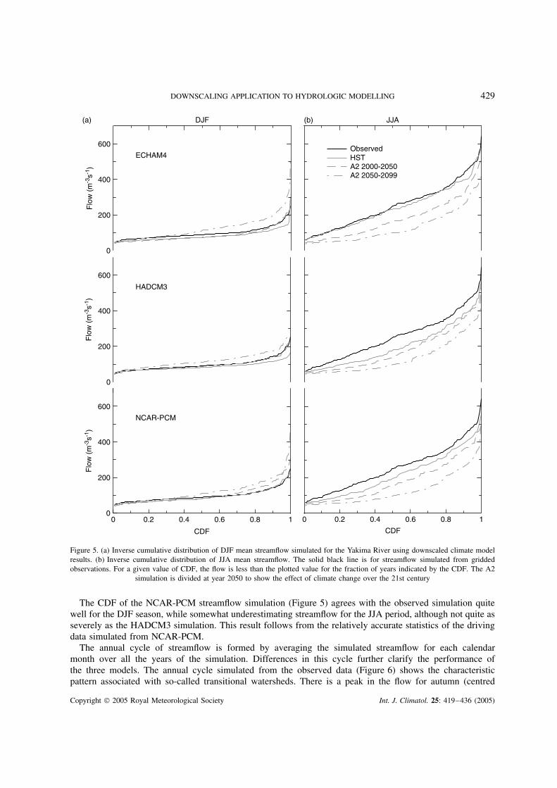
Streamflow computed from the ECHAM4 simulation produces a very close match to the observeddistribution of monthly flows for both seasons (Figure 5). This simulation shows a slight tendency tounderestimate flows for DJF, but is quite close to the observed distribution for JJA.

The HADCM3 simulation, however, produces much lower peak monthly flows (Figure 5). This disparityfollows from the deficiencies in the statistical distribution of simulated temperature for both DJF and JJA(Figures 3(a) and 4(a)). DJF temperatures control whether precipitation falls as snow or as rain; snow producesa snowpack that melts into the basin during summer, whereas rain immediately contributes to streamflow. Thus,the lack of warmer DJF events in HADCM3 (Figure 3(a)) would result in fewer rain-driven peaks in wintertimeflow. JJA temperatures control the rate at which the snowpack melts, which produces the summertime flow.



0 0.2 0.4 0.6 0.8

CDF

0

200

400

600

Flo

w (

m-3

s-1)

0

200

400

600

Flo

w (

m-3

s-1)

0

200

400

600

Flo

w (

m-3

s-1)

DJF

ObservedHSTA2 2000-2050A2 2050-2099

JJA

ECHAM4

NCAR-PCM

HADCM3

(a) (b)

1 0 0.2 0.4 0.6 0.8

CDF

1

Figure 5. (a) Inverse cumulative distribution of DJF mean streamflow simulated for the Yakima River using downscaled climate modelresults. (b) Inverse cumulative distribution of JJA mean streamflow. The solid black line is for streamflow simulated from griddedobservations. For a given value of CDF, the flow is less than the plotted value for the fraction of years indicated by the CDF. The A2

simulation is divided at year 2050 to show the effect of climate change over the 21st century

The CDF of the NCAR-PCM streamflow simulation (Figure 5) agrees with the observed simulation quitewell for the DJF season, while somewhat underestimating streamflow for the JJA period, although not quite asseverely as the HADCM3 simulation. This result follows from the relatively accurate statistics of the drivingdata simulated from NCAR-PCM.

The annual cycle of streamflow is formed by averaging the simulated streamflow for each calendarmonth over all the years of the simulation. Differences in this cycle further clarify the performance ofthe three models. The annual cycle simulated from the observed data (Figure 6) shows the characteristicpattern associated with so-called transitional watersheds. There is a peak in the flow for autumn (centred



0

100

200

300

400

Ann

ual C

ycle

of S

trea

mflo

w (

m-3

s-1)

ObservedHSTA2 2000-2050A2 2050-2100

ECHAM4

Jan Feb Mar Apr May Jun Jul Aug Sep Oct Nov Dec0

100

200

300

400

Ann

ual C

ycle

of S

trea

mflo

w (

m-3

s-1)

NCAR-PCM

0

100

200

300

400

Ann

ual C

ycle

of S

trea

mflo

w (

m-3

s-1)

HADCM3

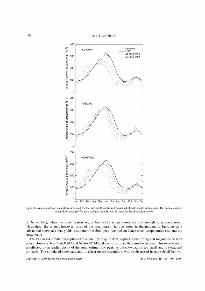
Figure 6. Annual cycle of streamflow simulated for the Yakima River from downscaled climate model simulations. The annual cycle isstreamflow averaged for each calendar month over all years in the simulation period

on November), when the rainy season begins but before temperatures are low enough to produce snow.Throughout the winter, however, most of the precipitation falls as snow in the mountains, building up asubstantial snowpack that yields a summertime flow peak (centred on June) when temperatures rise and thesnow melts.

The ECHAM4 simulation captures the annual cycle quite well, capturing the timing and magnitude of bothpeaks. However, both HADCM3 and NCAR-PCM tend to overestimate the rain-driven peak. This overestimateis reflected by an earlier decay of the summertime flow peak, as the snowpack is too small and is exhaustedtoo early. The simulated snowpack and its effect on the streamflow will be discussed in more detail below.



4. CLIMATE-CHANGE SIMULATIONS

4.1. Basin-mean precipitation and temperature

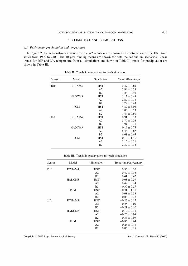
In Figure 2, the seasonal-mean values for the A2 scenario are shown as a continuation of the HST timeseries from 1990 to 2100. The 10-year running means are shown for both the A2 and B2 scenarios. Lineartrends for DJF and JJA temperature from all simulations are shown in Table II; trends for precipitation areshown in Table III.

Table II. Trends in temperature for each simulation

Season Model Simulation Trend (K/century)

DJF ECHAM4 HST 0.37 ± 0.69A2 3.94 ± 0.39B2 3.23 ± 0.49

HADCM3 HST 1.12 ± 0.49A2 2.87 ± 0.38B2 1.79 ± 0.43

PCM HST −4.89 ± 3.06A2 3.05 ± 0.53B2 1.44 ± 0.60

JJA ECHAM4 HST 0.91 ± 0.33A2 5.70 ± 0.26B2 3.94 ± 0.31

HADCM3 HST −0.19 ± 0.75A2 8.36 ± 0.62B2 6.61 ± 0.65

PCM HST −0.13 ± 1.46A2 3.15 ± 0.31B2 2.39 ± 0.32

Table III. Trends in precipitation for each simulation

Season Model Simulation Trend (mm/day/century)

DJF ECHAM4 HST 0.35 ± 0.50A2 0.42 ± 0.36B2 0.41 ± 0.42

HADCM3 HST 0.08 ± 0.39A2 0.42 ± 0.24B2 −0.30 ± 0.27

PCM HST −0.31 ± 1.70A2 0.08 ± 0.33B2 −0.08 ± 0.38

JJA ECHAM4 HST −0.23 ± 0.17A2 −0.25 ± 0.09B2 −0.21 ± 0.10

HADCM3 HST −0.10 ± 0.11A2 −0.26 ± 0.08B2 −0.36 ± 0.07

PCM HST −0.85 ± 0.64A2 −0.23 ± 0.11B2 0.06 ± 0.15



Whereas the ECHAM4-simulated DJF surface temperature shows little overall trend during the HSTsimulation (1900–90), there is significant warming simulated for the 21st century, particularly in the latterhalf of the century. This trend is illustrated by the 10-year running means (Figure 2). The CDFs show thetemperature increases uniformly, as the CDF maintains a similar shape (Figure 3a). Precipitation, however,shows relatively little trend for DJF in this simulation. Precipitation CDFs indicate a slight tendency to higherDJF precipitation simulated for 2050–2100 (Figure 3(b)).

The time series of results for downscaling the B2 forcing scenario are shown in Figure 2; for clarity, onlythe 10-year running mean is shown. There is very little difference between the results for the A2 and B2scenarios in both temperature and precipitation, either in the overall trend or in the CDFs (B2 CDFs are notshown).

For JJA, the ECHAM4 simulation yields trends in temperature and precipitation that are much moresignificant than for DJF (Figure 2). For the period 2050–2100, the coolest years are warmer than the warmestyears simulated for the 20th century (Figure 4(a)). Of the years from 2050–2100, 50% show precipitationless than the driest 7% of the years in the HST simulation (Figure 4(b)). The wettest years simulated for 21stcentury decrease less dramatically, with years comparable to the wettest simulated for the 20th century beingsimulated into the middle of the 21st century.

The trends in temperature and precipitation for the HADCM3 simulation are similar to ECHAM4 exceptfor JJA precipitation, where the trends for HADCM3 are much less severe than for ECHAM4. Similar resultsare found for NCAR-PCM, with comparable changes in temperature and smaller changes in JJA precipitationthan for ECHAM4.

Thus, taken alone, the changes in temperature would tend to alter streamflow by steadily reducing snowpackand increasing evapotranspiration. The effects of precipitation on streamflow would be minimal, with a slighttendency to reduce the severity of dry years. Although simulated JJA precipitation decreases dramatically,JJA precipitation is so small compared with the annual total that it has little effect on streamflow. Waterdemand, which is not considered here, could be altered significantly. The interaction of the temperature andprecipitation effects will only become clear when the results are used to force a hydrologic model, which isdiscussed in the following section.

4.2. Streamflow

The downscaled results from the simulation of future climate change are applied to simulating streamflowon the Yakima River as for the historic climate simulation discussed in Section 3.2. There is little qualitativedifference between the streamflow results for the A2 and B2 scenarios; hence, for clarity, only results for theA2 scenario are discussed here.

For all three climate models, comparisons of the CDFs of simulated streamflow show small increases inDJF flow (Figure 5(a)) and substantial reductions in JJA flows (Figure 5(b)) for the 21st century. The JJAreduction is greatest for the ECHAM4 and NCAR-PCM simulations. In both simulations, JJA flows thatare met for 50% of the years in the HST simulations are not met for 80% or more of the years in thesimulations for 2050–2100. The reduction in flow is a result of warming, not of precipitation, since thetrend in precipitation is quite flat for all models (Figure 2). The warming redistributes the flow within theannual cycle, but the total annual flow remains essentially constant over the two centuries in all models. Theannual cycle of streamflow for the climate-change scenarios (Figure 6) illustrates this shift in the flow peak.High flows begin much earlier in the year for the 21st century simulations, yielding a much broader peakto the annual cycle. The summertime peak shifts into spring, and August–September flows are substantiallyreduced. This effect is strongest in the ECHAM4 and NCAR-PCM simulations, which also reproduce morerealistic historic flows than HADCM3.

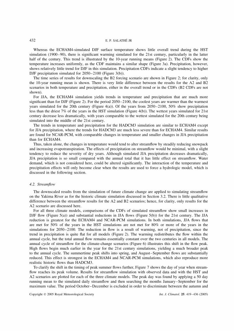
To clarify the shift in the timing of peak summer flows further, Figure 7 shows the day of year when stream-flow reaches its peak volume. Results for streamflow simulation with observed data and with the HST andA2 scenarios are plotted for each of the three climate models. The peak day was found by applying a 50 dayrunning mean to the simulated daily streamflow and then searching the months January–September for themaximum value. The period October–December is excluded in order to discriminate between the autumn and



Feb

Mar

Apr

May

Jun

Jul ECHAM4

Feb

Mar

Apr

May

Jun

Jul

Mon

th o

f Pea

k S

umm

er F

low HADCM3

Feb

Mar

Apr

May

Jun

Jul

ObservationsHSTA2

NCAR-PCM

1900 1950 2000 2050 2100

Year

Figure 7. Calendar day of the peak in the summer, melt-driven flow simulated for the Yakima River. The peak flow occurs earlier overthe course of the 21st century

summer flow peaks. The peak flow is typically simulated to occur in June for the observed data. ECHAM4 andNCAR-PCM HST simulations likewise produce typical peak flow days in June, but the HADCM3 HST simu-lation yields slightly earlier peak flows. For the A2 simulations, both ECHAM4 and NCAR-PCM shift the peakflow day 2–2.5 months earlier by the end of the 21st century; the shift for HADCM3 is only about a month.

4.3. Snowpack

As discussed in the analysis of the driving data above, ECHAM4 and HADCM3 have comparablesummertime warming, so the weaker response of flow timing in HADCM3 is more complex than a perturbationto the rate of summer warming. Rather, it appears that the excessive flow for DJF in the HADCM3 HST



simulation translates to weak sensitivity of the summer flow timing to warming. Excessive winter flowsuggests less precipitation is being stored in the snowpack during the rainy season.

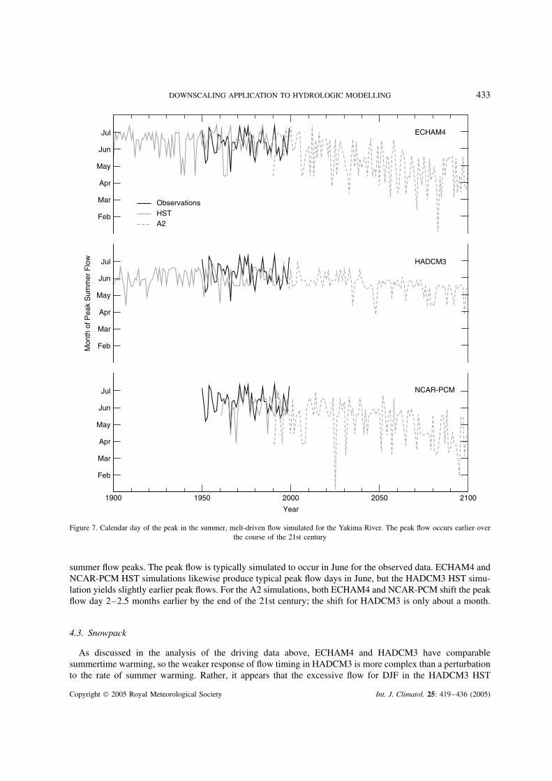
A deficit in snow storage is confirmed by the differences in the snow depth simulated by VIC for theECHAM4 and HADCM3 downscaled data. Figure 8 shows snow water equivalence (i.e. the depth of water ifthe snow were melted) from the ECHAM4 simulation minus the HADCM3 simulation for 1 April (Figure 8(a))and for 1 July (Figure 8(b)); contour lines indicate the topography, which generally slopes upward from eastto west.

On 1 April (Figure 8(a)), when the snowpack is near its maximum extent, the ECHAM4 historic simulationproduces much more snow at higher elevations compared with the HADCM3 simulation, and the HADCM3simulation has a slightly more snow at mid elevations. The actual snow line is very similar for both simulations.The lower elevation snow, where the two simulations are comparable, is melted off earlier in the season andis not the most significant fraction of the snowpack for summer flows. By 1 July (Figure 8(b)), the snowpackis nearly exhausted in HADCM3, but ECHAM4 still retains storage that contributes to flows into the latesummer. In this respect, ECHAM4 is much closer to observations. This remaining summertime snowpackis responsible for much of the sensitivity of streamflow to simulated future warming. In the ECHAM4 A2simulation, the summer snowpack is progressively diminished as summer temperatures rise over the basin. Inthe HADCM3 A2 simulation, since there is less snowpack simulated for present-day conditions, the warmingtrend cannot exert as much influence on the flow.

The disparity in snowpack is not due to differences in average temperature and precipitation during the rainyseason — the downscaling method forces these to be the same as for observations. To build up snowpack in

July(a) (b)

∆ Snow-waterEquivalent

(mm)

-1 1 25 75 150

500

1000

1000

500

1500

1500

500

1000

1000

500

1500

1500

47N

46N

121W 120W 121W 120W

47N

46N

April

Figure 8. Snow depth simulated for the Yakima River using ECHAM4 historic-run results minus snow depth simulated usingHADCM3historic-run results for (a) 1 April and (b) 1 July. Shading indicate snow depth in millimetres of snow water equivalent(i.e. the depth of water if the snow were melted). Contour lines indicate the topographic relief in metres, which slopes upward from

east to west



the autumn and winter rainy season, low temperatures must coincide with high-precipitation events, otherwisethe precipitation falls as rain and contributes immediately to streamflow. This basin is transitional betweenrain and snow dominance, and small variations in the autumn and winter temperatures can produce largeshifts in the amount of snow or rain that falls.

The difference between the snowpacks derived from the HADCM3 and ECHAM4 historic simulationsfollows from the CDFs for winter temperatures. ECHAM4 has a smaller range in temperature than HADCM3.The more frequent warm winters simulated by HADCM3 yield less snow than is simulated for ECHAM4,as is reflected in the greater snow water equivalent values from ECHAM4 (Figure 8). On the other hand,the more frequent cold winters in HADCM3 permit snow to be simulated for lower elevations more oftenthan for ECHAM4. This low-elevation snow is reflected in the lower snow amounts for ECHAM4 relativeto HADCM3 at mid elevations. Low-elevation snow pack, however, has less overall influence on the annualcycle of streamflow. Thus, this deficiency in the downscaled HADCM3 simulation of winter temperaturetranslates into an unrealistic annual cycle of streamflow. As a result, the simulated response of streamflow toclimate-change scenarios is weaker for HADCM3 than for the ECHAM4 and NCAR-PCM, which simulatea more realistic annual cycle.

5. DISCUSSION

The downscaling method applied to climate models in this paper is a very simple scaling of precipitationand temperature that forces the seasonal mean values simulated for present-day conditions to agree withobservations. The physical basis of the scaling is well founded, given the meteorology and topography of theregion. The large-scale weather systems that produce monthly variability in temperature and precipitation arewell resolved by global models. Although the mesoscale processes that produce the regional patterns are notcaptured by global models, these patterns are produced predominately by the interaction of the large-scalesystems with the stationary topography.

This minimal approach to downscaling requires that the global model simulates realistic interannualvariability. Other downscaling methods, such as bias correction, could constrain the temperature andprecipitation CDFs for the HST simulations to match the CDFs of observed temperature and precipitation.Thus, the issues that cause the HADCM3 simulations to yield poor simulated streamflow could be largelymitigated. However, doing so may obscure important deficiencies in how the model simulates the localweather dynamics and make model selection more difficult. If a model simulates present-day variabilityrealistically, then that performance gives more confidence to the model’s response to anthropogenic forcing.The simple local scaling exposes the capacity of the model simulation and allows one to judge which modelbest represents the conditions for a particular region under consideration. Since one of the models consideredhere, ECHAM4, performs quite well with even this simple downscaling, the ability to judge that performancemay well outweigh the benefits of a more sophisticated downscaling.

The ECHAM4 appears to do well in capturing the timing and distribution of precipitation events, and therelationship between precipitation events and temperature variability. The HADCM3 simulation for historicconditions appears to simulate unrealistic wintertime variability, which translates into less high-altitude snow,more wintertime streamflow, and an earlier peak to the summer flow compared with streamflow computedfrom observed data. As a result, the response of streamflow to climate change computed from the HADCM3A2 simulation is relatively weak compared with the streamflow computed from the ECHAM4 A2 scenario.The NCAR-PCM simulations fall between these two.

The good performance of ECHAM4 for the present-day simulation gives more confidence that the modeldoes a good job capturing the basic physical mechanisms of Pacific Northwest climate and, therefore, of thesensitivity of the region to climate change. This evaluation, however, does not address the global climateresponse of the model, which depends on processes not considered in a regional study. For the A2 scenario, theECHAM4 model simulates considerable warming for the region for summer. Simulated winter temperaturesincrease less dramatically. Simulated precipitation does not change significantly for either season with climatechange. The most significant response of streamflow in the Yakima River basin to these changes is a shift inthe typical summer flow peak from June to April during the 21st century.



ACKNOWLEDGEMENTS

Alan Hamlet provided assistance in obtaining and running the VIC hydrology model. Robert Norheim assistedin preparing figures of geographic data. This publication is funded by the Joint Institute for the Study of theAtmosphere and Ocean (JISAO) under NOAA Cooperative Agreement No. NA17RJ1232, contribution #1018.

REFERENCES

Daly C, Neilson RP, Phillips DL. 1994. A statistical topographic model for mapping climatological precipitation over mountainousterrain. Journal of Applied Meteorology 33: 140–158.

Giorgi F, Hewitson B, Christensen J, Hulme M, von Storch H, Whetton P, Jones R, Mearns L, Fu C. 2001. Regional climatesimulation — evaluation and projections. In Climate Change 2001: The Scientific Basis third assessment report, Houghton JT, Ding Y,Griggs DJ, Noguer M, van der Linden PJ, Dai X, Maskell K, Johnson CA (eds). Cambridge University Press: 583–638.

Gregory JM, Lowe JA. 2000. Predictions of global and regional sea-level rise using AOGCMs with and without flux adjustment.Geophysical Research Letters 27: 3069–3072.

Hamlet AF, Lettenmaier DP. 1999. Effects of climate change on hydrology and water resources in the Columbia River basin. Journalof the American Water Resources Association 35: 1597–1623.

Hay LE, Wilby RJL, Leavesley GH. 2000. A comparison of delta change and downscaled GCM scenarios for three mountainous basinsin the United States. Journal of the American Water Resources Association 36: 387–397.

Hay LE, Clark MP, Wilby RL, Gutowski WJ, Leavesley GH, Pan Z, Arritt RW, Takle ES. 2002. Use of regional climate model outputfor hydrologic simulations. Journal of Hydrometeorology 3: 571–590.

Houghton JT, Ding Y, Griggs DJ, Noguer M, van der Linden PJ, Dai X, Maskell K, Johnson CA (eds). 2001. Climate Change 2001:The Scientific Basis. Cambridge University Press: Cambridge (UK) and New York (USA).

Johns TC, Gregory JM, Ingram WJ, Johnson CE, Jones A, Lowe JA, Mitchell JFB, Roberts DL, Sexton DHM, Stevenson DS, Tett SFB,Woodge MJ. 2001. Anthropogenic climate change for 1860 to 2100 simulated with the HadCM3 model under updated emissionsscenarios. Hadley Centre Technical Note 22. The Hadley Centre for Climate Prediction and Research, The Met Office, Bracknell,UK.

Liang X, Lettenmaier DP, Wood EF, Burges SJ. 1994. A simple hydrologically based model of land-surface water and energy fluxesfor general-circulation models. Journal of Geophysical Research–Atmospheres 99: 14 415–14 428.

Lohmann D, NolteHolube R, Raschke E. 1996. A large-scale horizontal routing model to be coupled to land surface parametrizationschemes. Tellus Series A: Dynamic Meteorology and Oceanography 48: 708–721.

Lohmann D, Raschke E, Nijssen B, Lettenmaier DP. 1998. Regional scale hydrology: I. Formulation of the VIC-2l model coupled toa routing model. Hydrological Sciences Journal–Journal Des Sciences Hydrologiques 43: 131–141.

Matheussen B, Kirschbaum RL, Goodman IA, O’Donnell GM, Lettenmaier DP. 2000. Effects of land cover change on streamflow inthe interior Columbia River basin (USA and Canada). Hydrological Processes 14: 867–885.

Maurer EP, Wood AW, Adam JC, Lettenmaier DP, Nijssen B. 2002. A long-term hydrologically based dataset of land surface fluxesand states for the conterminous United States. Journal of Climate 15: 3237–3251.

Meehl GA, Gent PR, Arblaster JM, Otto-Bliesner BL, Brady EC, Craig A. 2001. Factors that affect the amplitude of El Nino in globalcoupled climate models. Climate Dynamics 17: 515–526.

Mitchell JFB, Johns TC, Senior CA. 1998. Transient response to increasing greenhouse gases using models with and without fluxadjustment. Hadley Centre Technical Note 2. The Hadley Centre for Climate Prediction and Research, The Met Office, Bracknell,UK.

Nakicenovic N, Alcamo J, Davis G, de Vries B, Fenhann J, Gaffin S, Gregory K, Grubler A, Jung TY, Kram T, La Rovere EL,Michaelis L, Mori S, Morita T, Pepper W, Pitcher H, Price L, Raihi K, Roehrl A, Rogner H-H, Sankovski A, Schlesinger MShukla P, Smith S, Swart R, van Rooijen S, Victor N, Dadi Z. 2000. IPCC Special Report on Emissions Scenarios. CambridgeUniversity Press: Cambridge (UK) and New York (USA).

Roeckner E, Bengtsson L, Feichter J, Lelieveld J, Rodhe H. 1999. Transient climate change simulations with a coupledatmosphere–ocean GCM including the tropospheric sulfur cycle. Journal of Climate 12: 3004–3032.

Salathe EP. 2003. Comparison of various precipitation downscaling methods for the simulation of streamflow in a rainshadow riverbasin. International Journal of Climatology 23: 887–901.

Stendel M, Schmith T, Roeckner E, Cubasch U. 2000. The climate of the 21st century: transient simulations with a coupledatmosphere–ocean general circulation model. Danmarks Klimacenter Report 00–6.

Washington WM, Weatherly JW, Meehl GA, Semtner AJ, Bettge TW, Craig AP, Strand WG, Arblaster J, Wayland VB, James R,Zhang Y. 2000. Parallel climate model (PCM) control and transient simulations. Climate Dynamics 16: 755–774.

Widmann M, Bretherton CS. 2000. Validation of mesoscale precipitation in the NCEP reanalysis using a new gridcell dataset for thenorthwestern United States. Journal of Climate 13: 1936–1950.

Widmann M, Bretherton CS, Salathe EP. 2003. Statistical precipitation downscaling over the northwestern United States usingnumerically simulated precipitation as a predictor. Journal of Climate 16: 799–816.

Wilby RL, Wigley TML. 2000. Precipitation predictors for downscaling: observed and general circulation model relationships.International Journal of Climatology 20: 641–661.

Wilby RL, Wigley TML, Conway D, Jones PD, Hewitson BC, Main J, Wilks DS. 1998. Statistical downscaling of general circulationmodel output: a comparison of methods. Water Resources Research 34: 2995–3008.

Wood AW, Maurer EP, Kumar A, Lettenmaier DP. 2002. Long-range experimental hydrologic forecasting for the eastern United States.Journal of Geophysical Research–Atmospheres 107: 4429–4443.


Documents

Downscaling simulations of future global climate with application to