Available online at www.sciencedirect.com

www.elsevier.com/locate/advwatres

Advances in Water Resources 31 (2008) 132–146

Statistical downscaling of GCM simulations to streamflowusing relevance vector machine

Subimal Ghosh, P.P. Mujumdar *

Department of Civil Engineering, Indian Institute of Science, Bangalore, Karnataka 560 012, India

Received 21 February 2007; received in revised form 20 July 2007; accepted 25 July 2007Available online 15 August 2007

Abstract

General circulation models (GCMs), the climate models often used in assessing the impact of climate change, operate on a coarse scaleand thus the simulation results obtained from GCMs are not particularly useful in a comparatively smaller river basin scale hydrology.The article presents a methodology of statistical downscaling based on sparse Bayesian learning and Relevance Vector Machine (RVM)to model streamflow at river basin scale for monsoon period (June, July, August, September) using GCM simulated climatic variables.NCEP/NCAR reanalysis data have been used for training the model to establish a statistical relationship between streamflow and cli-matic variables. The relationship thus obtained is used to project the future streamflow from GCM simulations. The statistical method-ology involves principal component analysis, fuzzy clustering and RVM. Different kernel functions are used for comparison purpose.The model is applied to Mahanadi river basin in India. The results obtained using RVM are compared with those of state-of-the-artSupport Vector Machine (SVM) to present the advantages of RVMs over SVMs. A decreasing trend is observed for monsoon streamflowof Mahanadi due to high surface warming in future, with the CCSR/NIES GCM and B2 scenario.� 2007 Elsevier Ltd. All rights reserved.

Keywords: GCM; Statistical downscaling; Relevance vector machine; Streamflow

1. Introduction

Modeling hydrologic impacts of climate change involvessimulation results from General Circulation Models(GCMs), which are the most credible tools designed to sim-ulate time series of climate variables globally, accountingfor the effects of greenhouse gases in the atmosphere.GCMs perform reasonably well in simulating climatic vari-ables at larger spatial scale (>104 km2), but poorly at thesmaller space and time scales relevant to regional impactanalyses [5]. Such poor performances of GCMs at localand regional scales have led to the development of LimitedArea Models (LAMs) in which fine computational gridover a limited domain is nested within the coarse grid ofa GCM [24]. This procedure is also known as dynamic

0309-1708/$ - see front matter � 2007 Elsevier Ltd. All rights reserved.

doi:10.1016/j.advwatres.2007.07.005

* Corresponding author. Tel.: +91 80 2360 0290; fax: +91 80 2360 0290.E-mail addresses: subimal@civil.iisc.ernet.in (S. Ghosh), pradeep@

civil.iisc.ernet.in (P.P. Mujumdar).

downscaling. The major drawback of dynamic downscal-ing, which restricts its use in climate change impact studies,is its complicated design and high computational cost.Moreover, it is inflexible in the sense that expanding theregion or moving to a slightly different region requiresredoing the entire experiment [11]. Another approach todownscaling, termed statistical downscaling, involvesderiving empirical relationships that transform large scalefeatures of the GCM (Predictors) to regional scale vari-ables (Predictands) such as precipitation and streamflow.There are three implicit assumptions involved in statisticaldownscaling [18]. Firstly, the predictors are variables of rel-evance and are realistically modeled by the host GCM. Sec-ondly, the empirical relationship is valid also under alteredclimatic conditions. Thirdly, the predictors employed fullyrepresent the climate change signal.

Statistical downscaling methodologies can be broadlyclassified into three categories [31,54]: weather generators,weather typing and transfer function. Weather generators

S. Ghosh, P.P. Mujumdar / Advances in Water Resources 31 (2008) 132–146 133

are statistical models of observed sequences of weathervariables. They can also be regarded as complex randomnumber generators, the output of which resembles dailyweather data at a particular location [26]. There are twofundamental types of daily weather generators, based onthe approach to model daily precipitation occurrence: theMarkov chain approach [21–23,30] and the spell-lengthapproach [56]. In the Markov chain approach, a randomprocess is constructed which determines a day at a stationas rainy or dry, conditional upon the state of the previousday, following given probabilities. In case of spell-lengthapproach, instead of simulating rainfall occurrences dayby day, spell-length models operate by fitting probabilitydistribution to observed relative frequencies of wet anddry spell lengths. In either case, the statistical parametersextracted from observed data are used along with somerandom components to generate a similar time series ofany length. Weather typing approaches [7] involve group-ing of local, meteorological variables in relation to differentclasses of atmospheric circulation. Future regional climatescenarios are constructed either by resampling from theobserved variable distribution (conditioned on the circula-tion pattern produced by a GCM), or by first generatingsynthetic sequences of weather pattern using Monte Carlotechniques and then resampling from the generated data.The mean, or frequency distribution of the local climateis then derived by weighting the local climate states withthe relative frequencies of the weather classes. The mostpopular approach of downscaling is the use of transfer

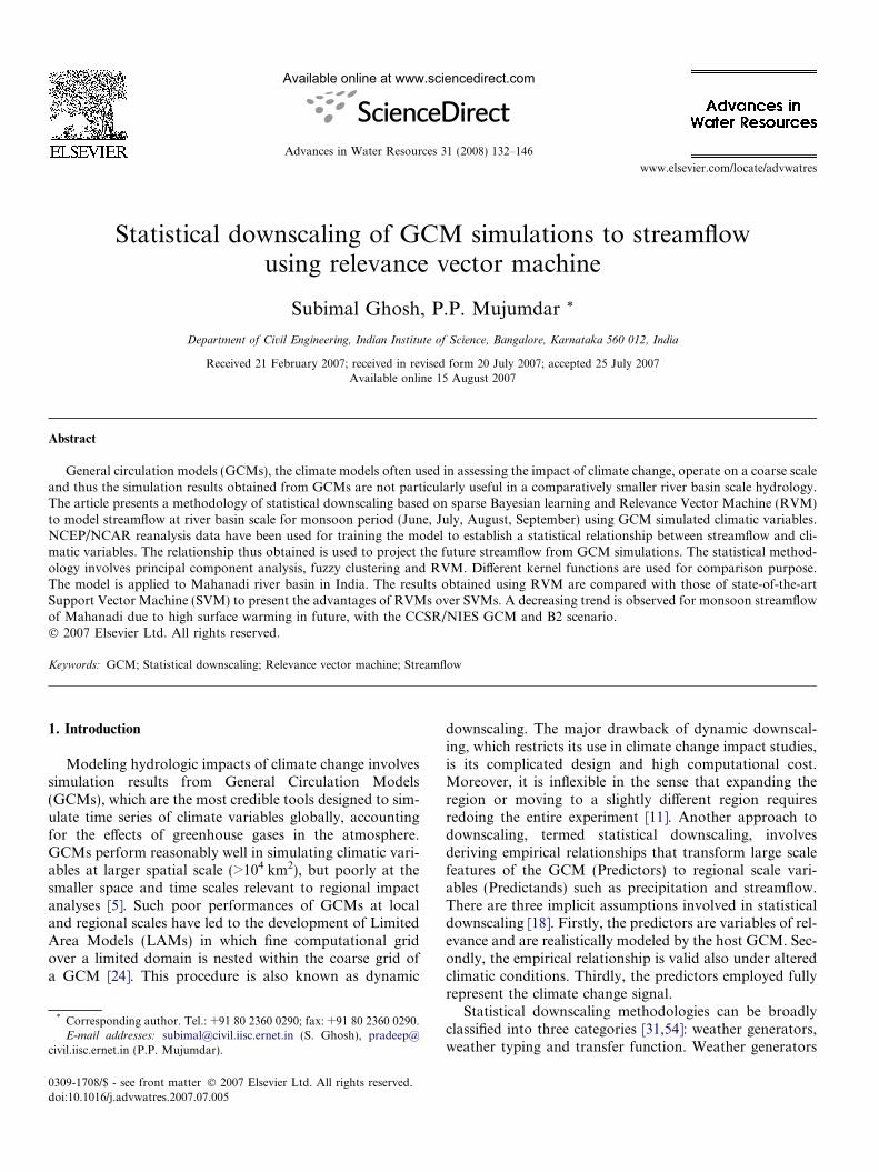
Fig. 1. Flowchart of th

function which is a regression based downscaling method[11,9,53,42] that relies on direct quantitative relationshipbetween the local scale climate variable (predictand) andthe variables containing the large scale climate information(predictors) through some form of regression. Individualdownscaling schemes differ according to the choice ofmathematical transfer function, predictor variables or sta-tistical fitting procedure. Todate, linear and nonlinearregression, Artificial Neural network (ANN), canonicalcorrelation, etc. have been used to derive predictor–predit-and relationship. Among them, ANN based downscalingtechniques have gained wide recognition owing to theirability to capture nonlinear relationships between predic-tors and predictand [11,19,45,41,51].

Despite a number of advantages, the traditional neuralnetwork models have several drawbacks including possibil-ity of getting trapped in local minima and subjectivity inthe choice of model architecture [43]. Recently, Vapnik[46,47] pioneered the development of a novel machinelearning algorithm, called Support Vector Machine(SVM), which provides an elegant solution to these prob-lems. The SVM has found wide range of applications inthe fields of classification and regression analysis. SVMhas some drawbacks of rapid increase of basis functionswith the size of training data set and absence of probabilis-tic interpretation [15]. Recently Tipping [44] developed Rel-evance Vector Machine (RVM), a new methodology forclassification and regression using the concept of probabi-listic bayesian learning framework, which can predict accu-

e proposed model.

134 S. Ghosh, P.P. Mujumdar / Advances in Water Resources 31 (2008) 132–146

rately utilizing dramatically fewer basis functions than acomparable SVM while offering a number of additionaladvantages.

In a recent study [42], SVM has been used as a down-scaling technique for predicting subdivisional precipitationof different regions in India. In that study, the GCM gen-erated large scale output (predictors) are converted intoprincipal components using Principal Component Analysis(PCA) and used directly as an input to SVM with GaussianRBF as the kernel function. Ghosh and Mujumdar [13]found that a heuristic classification of large scale GCMoutputs based on fuzzy clustering, prior to regression,improves the model performance and thus in the presentstudy both SVM and RVM coupled with PCA and fuzzyclustering are used to downscale GCM output to stream-flow. The flowchart of the model is presented in Fig. 1.The large scale GCM outputs are converted into principalcomponents using PCA, which is further classified intofuzzy clusters using fuzzy c-mean clustering. The member-ship in each of the clusters along with the principal compo-nents is used as input to SVM/RVM. The relationshipbetween the climate variables and streamflow is complexand nonlinear. Standard regression methods such as linearregression fail to model such nonlinear processes, andtherefore SVM and RVM are used in the present study.Gaussian RBF, Laplacian RBF and heavy tailed RBF havebeen used as the kernel functions to compare the results.The National Center for Environmental Prediction/National Center for Atmospheric Research (NCEP/NCAR) reanalysis data have been used for training thedownscaling model and GCM output is used for projectingfuture streamflow with the trained model. The performanceof RVM is compared with SVM for downscaling in thepresent study. Results are obtained with different kernelfunctions. The model is applied to the case study of Maha-nadi river basin in India to model the reservoir inflow tothe Hirakud dam from large scale GCM output. Details

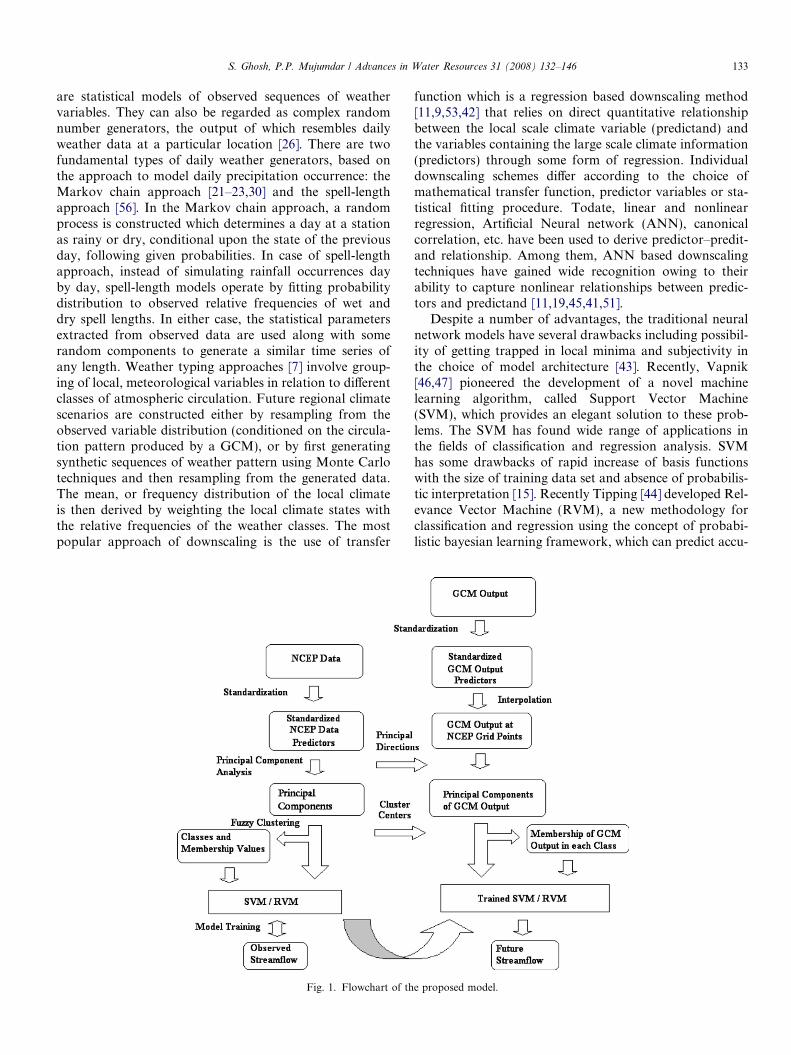
Fig. 2. NCEP grids superposed

of the case-study, data and the analysis performed priorto the training of SVM or RVM, is presented in the follow-ing section.

2. Data and input to vector machine

The Hirakud dam is located at Mahanadi River inOrissa at east coast of India (Fig. 2). The latitude andthe longitude of the location are 21.32�N and 83.45�E,respectively. The monthly inflow to Hirakud dam from1961 to 1990, is obtained from Department of Irrigation,Government of Orissa, India. Due to the absence of anymajor control structure upstream to Hirakud dam, theinflow to the dam is considered as unregulated flow. Maha-nadi is a rain-fed river with high streamflow in monsoon(June, July, August and September) due to heavy rainfalland therefore the ground water component with infiltrationis insignificant compared to the streamflow during themonsoon season. In the non-monsoon season, infiltrationto ground water is quite significant in absence of rainfall,resulting in low streamflow in Mahanadi with almost dryconditions. Thus, only for the monsoon season the stream-flow can be modeled with the climatological variables with-out considering ground water component. Therefore themonthly monsoon flow data of Mahanadi from year 1961to year 1990 is used in the downscaling model as predict-and. Selection of predictor is an important step in statisti-cal downscaling. The predictors, used for downscaling[49,52] should be: (1) reliably simulated by GCMs, (2) read-ily available from archives of GCM outputs, and (3)strongly correlated with the surface variables of interest.Cannon and Whitfield [9] have used MSLP, 500 hPa geo-potential height, 800 hPa specific humidity, and 100–500 hPa thickness field as the predictors for downscalingGCM output to streamflow. Monsoon streamflow can beconsidered broadly as the resultant of rainfall and evapora-tion. Rainfall is a consequence of Mean Sea Level Pressure

on Mahanadi River Basin.

S. Ghosh, P.P. Mujumdar / Advances in Water Resources 31 (2008) 132–146 135

(MSLP) [2,3,22,49], geopotential height and humiditywhereas evaporation is mainly guided by temperatureand humidity. Therefore, The present study considers 2 msurface air temperature, MSLP, 500 hPa geopotentialheight and surface specific humidity as the predictors formodeling Mahanadi streamflow in monsoon season. It isworth mentioning that land use is the single most impor-tant factor in generating the flow from the rainfall. In thepresent study, land use pattern is assumed to remain thesame in future and therefore the statistical relationshipbetween the predictors and the streamflow will remainunaltered in future. Gridded climate variables are obtainedfrom the National Center for Environmental Prediction/National Center for Atmospheric Research (NCEP/NCAR) reanalysis project [25] (http://www.cdc.noaa.gov/cdc/reanalysis/reanalysis.shtml). Reanalysis data are out-puts from a high resolution atmospheric model that hasbeen run using data assimilated from surface observationstations, upper-air stations, and satellite-observing plat-forms. Results obtained using these fields therefore repre-sent those that could be expected from an ideal GCM [9].Monthly climatological data from 1961 to 1990 wereobtained for a region spanning 15�N–25�N in latitudeand 80�E–90�E in longitude. Fig. 2 shows the NCEP gridpoints superposed on the map of Mahanadi river basin.A statistical relationship based on fuzzy clustering and vec-tor machine is developed between large scale climatic vari-ables and inflow to Hirakud dam, with reanalysis data asregressor and observed streamflow as regressand. This rela-tionship is used to model the future streamflow using GCMoutput. GCM developed by Center for Climate SystemResearch/ National Institute for Environmental Studies(CCSR/NIES), Japan, with B2 scenario is used for projec-tion of future streamflow. The grid size of the GCM is 5.5�latitude · 5.625� longitude. The monthly output for B2 sce-nario is extracted for CCSR–NIES GCM for the region ofinterest covering all the NCEP grid points extending from13.8445�N to 30.4576�N in latitude and 78.7500�E to95.6250�E in longitude from IPCC data distribution center(http://www.mad.zmaw.de/IPCC_DDC/html/ddc_gcmdata.html).

Standardization [54] is used prior to statistical down-scaling to reduce systematic biases in the mean and vari-ances of GCM outputs relative to the observations orNCEP/NCAR data. The procedure typically involves sub-traction of mean and division by standard deviation of thepredictor variable for a predefined baseline period for bothNCEP/NCAR and GCM output. The period 1961–1990 isused as a base-line because it is of sufficient duration toestablish a reliable climatology, yet not too long, nor toocontemporary to include a strong global change signal[54]. A major limitation of standardization is that it consid-ers the bias in only mean and variance. There is a possibil-ity that the reanalysis data and GCM output may deviatefrom normal distribution, and there may exist bias in otherstatistical parameters. For Mahanadi river basin, four pre-dictor variables (MSLP, 2 m surface air temperature, spe-

cific humidity, and 500hPa geopotential height) at 25NCEP grid points with a dimensionality of 100, are usedwhich are highly correlated with each other. PrincipalComponent Analysis (PCA) [21,13] is performed to trans-form the set of correlated N-dimensional predictors(N = 100) into another set of N-dimensional uncorrelatedvectors (called principal components) by linear combina-tion, such that most of the information content of the ori-ginal data set is stored in the first few dimensions of thenew set. In the present study, it is observed that first 10Principal Components (PCs) represent 98.1% of the infor-mation content (or variability) of the original predictors,and therefore they are used in downscaling. The advantageof PCA is that it reduces the dimensionality of the predic-tors and at the same time there is no redundant informa-tion and correlation among the predictors, which maylead to multicollinearity. Fuzzy clustering is used to classifythe principal components into classes or clusters. Fuzzyclustering assigns membership values of the classes to var-ious data points, and it is more generalized and useful todescribe a point not by a crisp cluster, but by its member-ship values in all the clusters [35,16].

The important parameters required for fuzzy clusteringalgorithm are number of clusters (c) and fuzzificationparameter (m). Fuzzification parameter controls the degreeof fuzziness of the resulting classification, which is thedegree of overlap between clusters. The minimum valueof m is 1 which implies hard clustering. Number of clustersand fuzzification parameter are determined from clustervalidity indices like Fuzziness Performance Index (FPI)and Normalized Classification Entropy (NCE) [36]. FPIestimates the degree of fuzziness generated by a specifiednumber of classes and is given by

FPI ¼ 1� cF � 1

c� 1ð1Þ

where

F ¼ 1

T

Xc

i¼1

XT

t¼1

ðlitÞ2 ð2Þ

lit is the membership in cluster i of the principal compo-nents in month t. NCE estimates the degree of disorganiza-tion created by a specified number of classes and given as

NCE ¼ Hlog c

ð3Þ

where

H ¼ 1

T

Xc

i¼1

XT

t¼1

�lit � logðlitÞ ð4Þ

The optimum number of classes/clusters is established onthe basis of minimizing these two measures given by Eqs.(1)–(3). The FPI and NCE attain their minimum valueswhen the number of clusters is 3 for almost all cases withdifferent m values. The value of FPI should be chosen insuch a way that the resulting clustering is neither too fuzzy

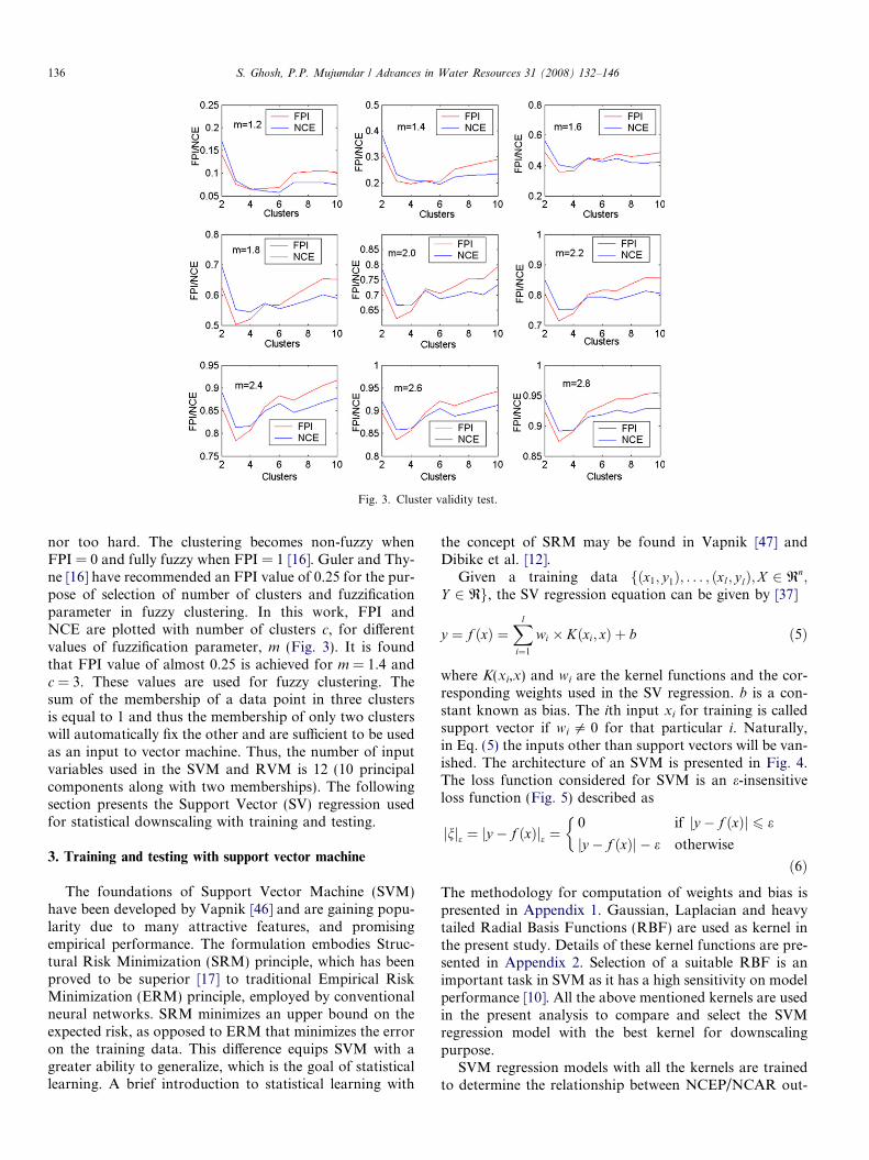
Fig. 3. Cluster validity test.

136 S. Ghosh, P.P. Mujumdar / Advances in Water Resources 31 (2008) 132–146

nor too hard. The clustering becomes non-fuzzy whenFPI = 0 and fully fuzzy when FPI = 1 [16]. Guler and Thy-ne [16] have recommended an FPI value of 0.25 for the pur-pose of selection of number of clusters and fuzzificationparameter in fuzzy clustering. In this work, FPI andNCE are plotted with number of clusters c, for differentvalues of fuzzification parameter, m (Fig. 3). It is foundthat FPI value of almost 0.25 is achieved for m = 1.4 andc = 3. These values are used for fuzzy clustering. Thesum of the membership of a data point in three clustersis equal to 1 and thus the membership of only two clusterswill automatically fix the other and are sufficient to be usedas an input to vector machine. Thus, the number of inputvariables used in the SVM and RVM is 12 (10 principalcomponents along with two memberships). The followingsection presents the Support Vector (SV) regression usedfor statistical downscaling with training and testing.

3. Training and testing with support vector machine

The foundations of Support Vector Machine (SVM)have been developed by Vapnik [46] and are gaining popu-larity due to many attractive features, and promisingempirical performance. The formulation embodies Struc-tural Risk Minimization (SRM) principle, which has beenproved to be superior [17] to traditional Empirical RiskMinimization (ERM) principle, employed by conventionalneural networks. SRM minimizes an upper bound on theexpected risk, as opposed to ERM that minimizes the erroron the training data. This difference equips SVM with agreater ability to generalize, which is the goal of statisticallearning. A brief introduction to statistical learning with

the concept of SRM may be found in Vapnik [47] andDibike et al. [12].

Given a training data fðx1; y1Þ; . . . ; ðxl; ylÞ;X 2 Rn;Y 2 Rg, the SV regression equation can be given by [37]

y ¼ f ðxÞ ¼Xl

i¼1

wi � Kðxi; xÞ þ b ð5Þ

where K(xi,x) and wi are the kernel functions and the cor-responding weights used in the SV regression. b is a con-stant known as bias. The ith input xi for training is calledsupport vector if wi 5 0 for that particular i. Naturally,in Eq. (5) the inputs other than support vectors will be van-ished. The architecture of an SVM is presented in Fig. 4.The loss function considered for SVM is an e-insensitiveloss function (Fig. 5) described as

jnje ¼ jy � f ðxÞje ¼0 if jy � f ðxÞj 6 e

jy � f ðxÞj � e otherwise

�ð6Þ

The methodology for computation of weights and bias ispresented in Appendix 1. Gaussian, Laplacian and heavytailed Radial Basis Functions (RBF) are used as kernel inthe present study. Details of these kernel functions are pre-sented in Appendix 2. Selection of a suitable RBF is animportant task in SVM as it has a high sensitivity on modelperformance [10]. All the above mentioned kernels are usedin the present analysis to compare and select the SVMregression model with the best kernel for downscalingpurpose.

SVM regression models with all the kernels are trainedto determine the relationship between NCEP/NCAR out-

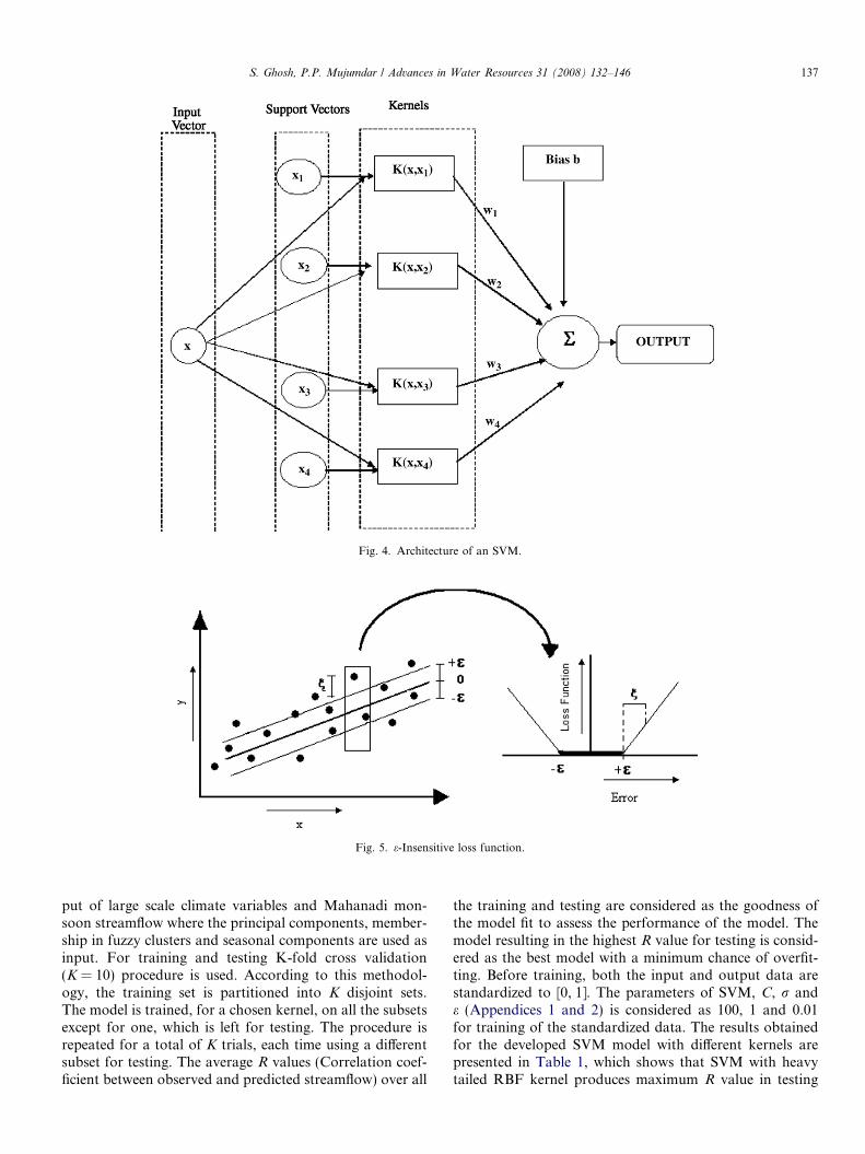
Fig. 4. Architecture of an SVM.

Fig. 5. e-Insensitive loss function.

S. Ghosh, P.P. Mujumdar / Advances in Water Resources 31 (2008) 132–146 137

put of large scale climate variables and Mahanadi mon-soon streamflow where the principal components, member-ship in fuzzy clusters and seasonal components are used asinput. For training and testing K-fold cross validation(K = 10) procedure is used. According to this methodol-ogy, the training set is partitioned into K disjoint sets.The model is trained, for a chosen kernel, on all the subsetsexcept for one, which is left for testing. The procedure isrepeated for a total of K trials, each time using a differentsubset for testing. The average R values (Correlation coef-ficient between observed and predicted streamflow) over all

the training and testing are considered as the goodness ofthe model fit to assess the performance of the model. Themodel resulting in the highest R value for testing is consid-ered as the best model with a minimum chance of overfit-ting. Before training, both the input and output data arestandardized to [0, 1]. The parameters of SVM, C, r ande (Appendices 1 and 2) is considered as 100, 1 and 0.01for training of the standardized data. The results obtainedfor the developed SVM model with different kernels arepresented in Table 1, which shows that SVM with heavytailed RBF kernel produces maximum R value in testing

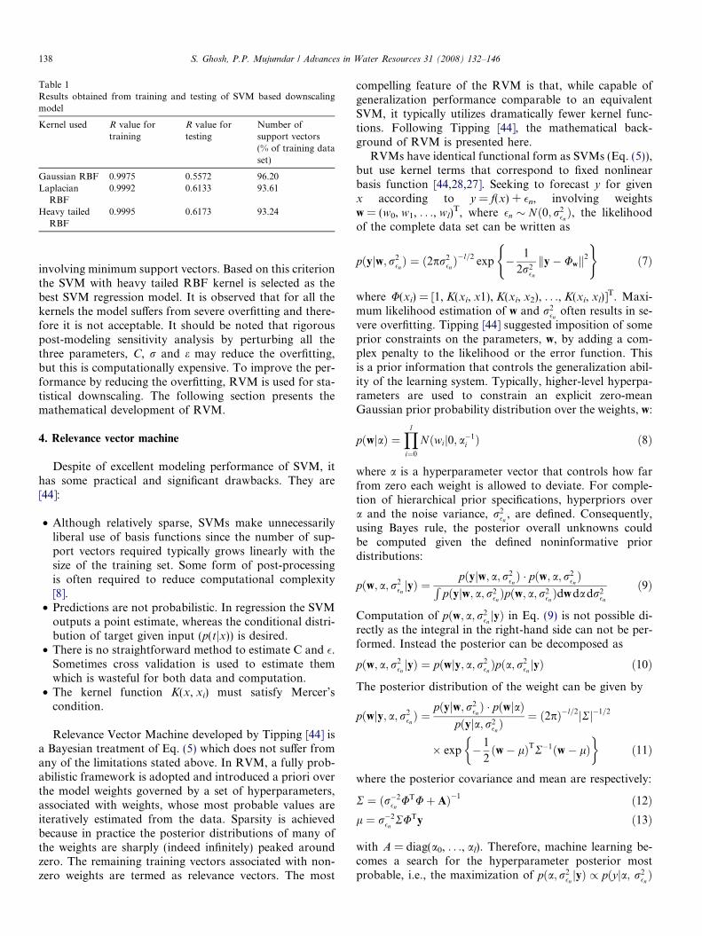
Table 1Results obtained from training and testing of SVM based downscalingmodel

Kernel used R value fortraining

R value fortesting

Number ofsupport vectors(% of training dataset)

Gaussian RBF 0.9975 0.5572 96.20Laplacian

RBF0.9992 0.6133 93.61

Heavy tailedRBF

0.9995 0.6173 93.24

138 S. Ghosh, P.P. Mujumdar / Advances in Water Resources 31 (2008) 132–146

involving minimum support vectors. Based on this criterionthe SVM with heavy tailed RBF kernel is selected as thebest SVM regression model. It is observed that for all thekernels the model suffers from severe overfitting and there-fore it is not acceptable. It should be noted that rigorouspost-modeling sensitivity analysis by perturbing all thethree parameters, C, r and e may reduce the overfitting,but this is computationally expensive. To improve the per-formance by reducing the overfitting, RVM is used for sta-tistical downscaling. The following section presents themathematical development of RVM.

4. Relevance vector machine

Despite of excellent modeling performance of SVM, ithas some practical and significant drawbacks. They are[44]:

• Although relatively sparse, SVMs make unnecessarilyliberal use of basis functions since the number of sup-port vectors required typically grows linearly with thesize of the training set. Some form of post-processingis often required to reduce computational complexity[8].

• Predictions are not probabilistic. In regression the SVMoutputs a point estimate, whereas the conditional distri-bution of target given input (p(tjx)) is desired.

• There is no straightforward method to estimate C and �.Sometimes cross validation is used to estimate themwhich is wasteful for both data and computation.

• The kernel function K(x, xi) must satisfy Mercer’scondition.

Relevance Vector Machine developed by Tipping [44] isa Bayesian treatment of Eq. (5) which does not suffer fromany of the limitations stated above. In RVM, a fully prob-abilistic framework is adopted and introduced a priori overthe model weights governed by a set of hyperparameters,associated with weights, whose most probable values areiteratively estimated from the data. Sparsity is achievedbecause in practice the posterior distributions of many ofthe weights are sharply (indeed infinitely) peaked aroundzero. The remaining training vectors associated with non-zero weights are termed as relevance vectors. The most

compelling feature of the RVM is that, while capable ofgeneralization performance comparable to an equivalentSVM, it typically utilizes dramatically fewer kernel func-tions. Following Tipping [44], the mathematical back-ground of RVM is presented here.

RVMs have identical functional form as SVMs (Eq. (5)),but use kernel terms that correspond to fixed nonlinearbasis function [44,28,27]. Seeking to forecast y for givenx according to y = f(x) + �n, involving weightsw = (w0, w1, . . ., wl)

T, where �n � Nð0; r2�nÞ, the likelihood

of the complete data set can be written as

pðyjw; r2�nÞ ¼ ð2pr2

�n�l=2 exp � 1

2r2�n

ky� Uwk2

( )ð7Þ

where U(xi) = [1, K(xi, x1), K(xi, x2), . . ., K(xi, xl)]T. Maxi-

mum likelihood estimation of w and r2�n

often results in se-vere overfitting. Tipping [44] suggested imposition of someprior constraints on the parameters, w, by adding a com-plex penalty to the likelihood or the error function. Thisis a prior information that controls the generalization abil-ity of the learning system. Typically, higher-level hyperpa-rameters are used to constrain an explicit zero-meanGaussian prior probability distribution over the weights, w:

pðwjaÞ ¼Yl

i¼0

Nðwij0; a�1i Þ ð8Þ

where a is a hyperparameter vector that controls how farfrom zero each weight is allowed to deviate. For comple-tion of hierarchical prior specifications, hyperpriors overa and the noise variance, r2

�n, are defined. Consequently,

using Bayes rule, the posterior overall unknowns couldbe computed given the defined noninformative priordistributions:

pðw; a; r2�njyÞ ¼

pðyjw; a; r2�nÞ � pðw; a; r2

�nÞR

pðyjw; a; r2�nÞpðw; a; r2

�nÞdwdadr2

�n

ð9Þ

Computation of pðw; a; r2�njyÞ in Eq. (9) is not possible di-

rectly as the integral in the right-hand side can not be per-formed. Instead the posterior can be decomposed as

pðw; a; r2�njyÞ ¼ pðwjy; a; r2

�nÞpða; r2

�njyÞ ð10Þ

The posterior distribution of the weight can be given by

pðwjy; a; r2�nÞ ¼

pðyjw; r2�nÞ � pðwjaÞ

pðyja; r2�nÞ ¼ ð2pÞ�l=2jRj�1=2

� exp � 1

2ðw� lÞTR�1ðw� lÞ

� �ð11Þ

where the posterior covariance and mean are respectively:

R ¼ ðr�2�n

UTUþ AÞ�1 ð12Þl ¼ r�2

�nRUTy ð13Þ

with A = diag(a0, . . ., al). Therefore, machine learning be-comes a search for the hyperparameter posterior mostprobable, i.e., the maximization of pða; r2

�njyÞ / pðyja; r2

�nÞ

Table 2Results obtained from training and testing of RVM based downscalingmodel

Kernel used R value fortraining

R value fortesting

Number ofrelevant vectors(% of training dataset)

Gaussian RBF 0.9423 0.6019 71.30Laplacian

RBF0.8417 0.6418 25.56

Heavy tailedRBF

0.7937 0.6998 8.06

S. Ghosh, P.P. Mujumdar / Advances in Water Resources 31 (2008) 132–146 139

pðaÞpðr2�nÞ with respect to a and r2

�n. For uniform hyperp-

riors, it is required to maximize the term pðyja; r2�nÞ, which

is computable and given by

pðyja; r2�nÞ ¼

Zpðyjw; r2

�nÞpðwjaÞdw

¼ ð2pÞ�l=2jr2�n

I þ UA�1UTj1=2

� expf� 1

2yTðr2

�nI þ UA�1UTÞ�1

yg ð14Þ

Tipping [44] contended that all the evidence from severalexperiments suggests that this predictive approximation isvery effective. Bayesian models refer to Eq. (9) as the mar-ginal likelihood, and its maximization is known as the typeII-maximum likelihood method [6,48]. As argued by Tip-ping [44], MacKay [29] refers to this term as the evidencefor hyperparameter and its maximization as the evidenceprocedure. Hyperparameter estimation is typically carriedout with an iterative formula such as a gradient ascenton the objective function [44,29].

At convergence of the hyperparameter estimation proce-dure, predictions can be made based on the posterior distri-bution over the weights, conditioned on the maximizedmost probable values of a and r2

�n, aMP and r2

MP respec-tively. The predictive distribution for a given x* can becomputed using Eq. (11):

pðy�jy; aMP; r2MPÞ ¼

Zpðy�jw; r2

MPÞpðwjy; aMP; r2MPÞdw

ð15ÞSince both terms in the integrand are Gaussian, this can bereadily computed, giving

pðy�jy; aMP; r2MPÞ ¼ Nðy�jt�; r2

�Þ ð16Þwith

t� ¼ lTUðx�Þ; ð17Þr2� ¼ r2

MP þ Uðx�ÞTRUðx�Þ ð18Þ

The outcome of the optimization involved in RVM (i.e.maximization of pðyja; r2

�nÞ), is that many elements of a

go to infinity such that w will have only a few nonzeroweights that will be considered as relevant vectors. The rel-evant vectors (RVs) can be viewed as counterparts to sup-port vectors (SVs) in SVMs; therefore, the resulting modelenjoys the properties of SVMs (i.e., sparsity and generaliza-tion) and, in addition, provides estimates of uncertaintybounds in the predictions they make [28].

4.1. Training and testing with RVM

Principal components and fuzzy cluster membershipsderived from NCEP/NCAR reanalysis data are used asinput to RVM. Similar to SVM, Gaussian RBF, LaplacianRBF and Heavy tailed RBF are used as kernels in theRVM regression model for downscaling with K-fold crossvalidation. The results obtained from training and testing

are presented, with r = 1, in Table 2. Compared to SVM,RVM involves very few relevant vectors for the regressionwith all the kernels and thus minimizing the possibility ofovertraining as well as computational time. This is reflectedin the differences between R values for training and testingwith all the kernels. A comparatively small differencebetween the R value of training and testing shows thereduction of overtraining which is not achieved by SVM.Among the RVM kernels the model with heavy tailedRBF shows the highest R value for testing among all theRVM models and thus selected as the best model for down-scaling. The selection of the width of the kernel is one ofthe major criterion in selecting the appropriate model.The kernel width can not be computed with the Bayesiantreatment of RVM and therefore a post-modeling sensitiv-ity analysis is required to compute kernel width that resultsin minimum overfitting. Sensitivity analysis of the trainingand testing R values and the number of RVs involved inthe model is carried out, with variation in the kernel width,and presented in Fig. 6. As RVM involves only kernelwidth as a parameter, the computational effort of post-modeling sensitivity analysis is significantly less comparedto SVM. It is observed that the testing R value achievedits maximum at a kernel width of 1.9, involving minimumnumber of RVs. The training and testing R values areobtained as 0.7745 and 0.7256, respectively, using only7.41% of the data set as relevant vectors. Therefore RVMusing heavy tailed RBF with the width of 1.9 is used forstatistical downscaling in the present study. After the selec-tion of model the whole data set is trained using RVMbased regression with heavy tailed RBF as the kernel.The overall R value is obtained as 0.8226. The observedand predicted monsoon streamflow from June 1961 toAugust 1990 with scatter plot are presented in Fig. 7. Itis clear that even RVM is not able to mimic the extremerainfall observed in the record. Possibly this could bebecause regression based statistical downscaling modelsoften cannot explain entire variance of the downscaled var-iable [54,42]. The goodness of fit of the model is also testedwith Nash–Sutcliffe coefficient [32], which has been recom-mended by ASCE Task Committee on definition of Crite-ria for evaluation of watershed models of the watershedmanagement committee, Irrigation and Drainage Division[1]. The Nash–Sutcliffe coefficient (E) is given by

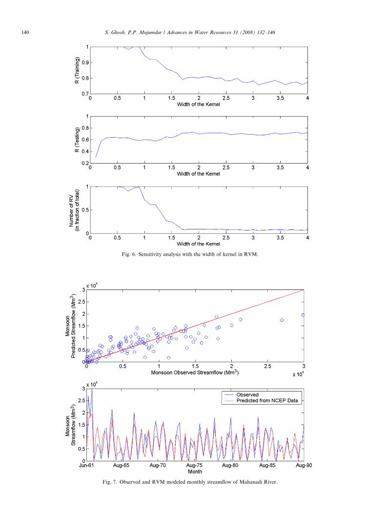
Fig. 6. Sensitivity analysis with the width of kernel in RVM.

Fig. 7. Observed and RVM modeled monthly streamflow of Mahanadi River.

140 S. Ghosh, P.P. Mujumdar / Advances in Water Resources 31 (2008) 132–146

S. Ghosh, P.P. Mujumdar / Advances in Water Resources 31 (2008) 132–146 141

E ¼ 1�P

tðQot � QptÞ2P

tðQot � QoÞ2

ð19Þ

where Qot and Qpt are the observed and predicted stream-flow in time t, and Qo is the mean observed streamflow.Nash–Sutcliffe coefficient can vary from 0 to 1 with 0 indi-cating that the model predics no better than the average ofthe observed data, and 1 indicating a perfect fit. It is ob-tained as 0.67 for the present model which is satisfactory.Wetterhall et al. [49] have tested the long term seasonalmean, and standard deviation for verification of a down-scaling model. In the present analysis also, similar testhas been performed. The long term mean and standarddeviation of observed streamflow are 7332.0 Mm3 and5995.6 Mm3 and those of predicted streamflow are7384.1 Mm3 and 4607.6 Mm3, which shows a good matchin mean but difference in standard deviation. This may bebecause the regression based statistical downscaling modelsoften cannot explain entire variance of the downscaled var-iable [54] and therefore the present model can not mimicthe high streamflow in 1961. Other limitation of the meth-od is that assuming constant error variance (homoscedasi-ty) may prove to be a limitation when streamflow is theresponse variable as it is often observed that streamflow er-ror variance is related to the magnitude of the flow, and,the hierarchical structure cannot accommodate Markoviandependence in the flows easily. After the verification, theRVM regression model is used for modeling of futurestreamflow time series from the predictor variables as pro-jected by GCM developed by CCSR/NIES with B2scenarios.

Fig. 8. Projected future Streamflow for CCSR/NIES GC

5. Future streamflow projection

GCM developed by Center for Climate System Research/National Institute for Environmental Studies (CCSR/NIES), Japan, with B2 scenario is used for projection offuture streamflow. The grid size of the GCM is 5.5�latitude · 5.625� longitude. The monthly output for B2scenario is extracted for CCSR/NIES GCM for the regionof interest covering all the NCEP grid points extending from13.8445�N to 30.4576�N in latitude and 78.7500�E to95.6250�E in longitude from IPCC data distribution center.GCM grid points do not match with NCEP grid points andthus interpolation is required to obtain the GCM output atNCEP grid points. Interpolation is performed with a linearinverse square procedure using spherical distances [57]. Thepredictor variables for CCSR/NIES GCM are then interpo-lated to the 25 NCEP grid points. Using the principal direc-tions or eigen vectors obtained from PCA of NCEP data,principal components are obtained for the GCM output.The membership of the principal components of GCMoutput in each of the fuzzy clusters are then computed usingthe cluster centers obtained from fuzzy clustering. Principalcomponents and cluster membership of GCM output arethen used in the developed RVM regression model to projectthe monsoon streamflow of Mahanadi for future.

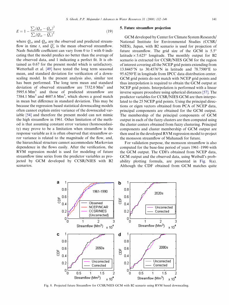
For validation purpose, the monsoon streamflow is alsocomputed for the base-line period of years 1961–1990 withthe GCM output. The CDFs obtained from NCEP data,GCM output and the observed data, using Weibull’s prob-ability plotting formula, are presented in Fig. 8(a).Although the CDF obtained from GCM matches quite

M with B2 scenario using RVM based downscaling.

142 S. Ghosh, P.P. Mujumdar / Advances in Water Resources 31 (2008) 132–146

well, there is considerable bias near zero flow values and atthe extreme cases. This is because standardisation mayreduce the bias in the mean and variance of the predictorvariable but it is much harder to accommodate the biasesin large scale patterns of atmospheric circulation in GCMs(e.g. shifts in the dominant storm track relative to observeddata) or unrealistic inter-variable relationships [50]. More-over, regression based statistical downscaling models oftencannot explain entire variance of the downscaled variable,which is also reflected in terms of bias near zero flow andhigh flow conditions. While modeling monsoon streamflowsuch biases should be taken care otherwise it will propagatein the computation of future seasons [14]. To remove suchbias from a given downscaled output the following meth-odology is used:

• CDFs are obtained with the downscaled GCM gener-ated and observed streamflow for the years 1961–1990using Weibull’s probability plotting position formula.

• For a given value of GCM generated streamflow(XGCM), the value of CDF (CDFGCM) is computed.

• Corresponding to CDFGCM the observed streamflowvalue is obtained from the CDF of observed data.

• The GCM generated streamflow is replaced by theobserved data, thus computed, having the same CDFvalue.

• The CDFs of GCM generated and observed streamflow,obtained for the years 1961–1990, act as reference, andbased on them the correction is applied to the stream-flow values obtained from GCM for future.

A major drawback of the method described above isthat, if the future GCM streamflow is out of the rangeof historical GCM streamflow, the methodology of biascorrection with Weibull’s plotting position will fail. If suchcases appear, then different parametric probability distri-bution (with upper bound of random variable as 1) canbe fitted to the observed GCM streamflow and the bestpdf can be selected among them with Akaike InformationCriteria (AIC) or v2-test. As the new range is nowextended to1, it is possible to perform the quantile trans-formation even if the future GCM streamflow is out of therange of historical GCM streamflow. In the present case,the future GCM streamflows are all within the range ofobserved GCM streamflow and therefore the bias is cor-rected with Weibull’s plotting position and quantile trans-formation. The long term mean and standard deviation ofobserved streamflow are 7332.0 Mm3 and 5995.6 Mm3 andthose of GCM projected streamflow before bias correctionwere 7194.2 Mm3 and 5607.2 Mm3. After bias correctionmean and standard deviation of GCM projected stream-flow are 7331.7 Mm3 and 6009.4 Mm3, respectively, whichshows bias has been significantly reduced. The CDFs pro-jected future streamflow is plotted for standard 30 yeartime slices 2020 s, 2050 s and 2080 s in Fig. 8b–d, whichclearly shows a decrease in the high flows of the monsoonseason in Mahanadi. The occurrence of extreme high flow

events will reduce significantly and therefore there is adecreasing trend in the monthly peak flow. The projectionof CCSR/NIES GCM with B2 scenario presents a favor-able condition for Hirakud dam in future for flood controloperation. Earlier study [34] on Mahanadi river alsorevealed decrease in monsoon streamflow for the historicperiod with an increasing trend in surface temperature.It is concluded in that study, that due to increase in tem-perature, the water yields in the river is adversely affected.Following the study, it can be inferred that one of theprobable reason of such decreasing trend in streamflowmay be significant increase in temperature due to climatewarming.

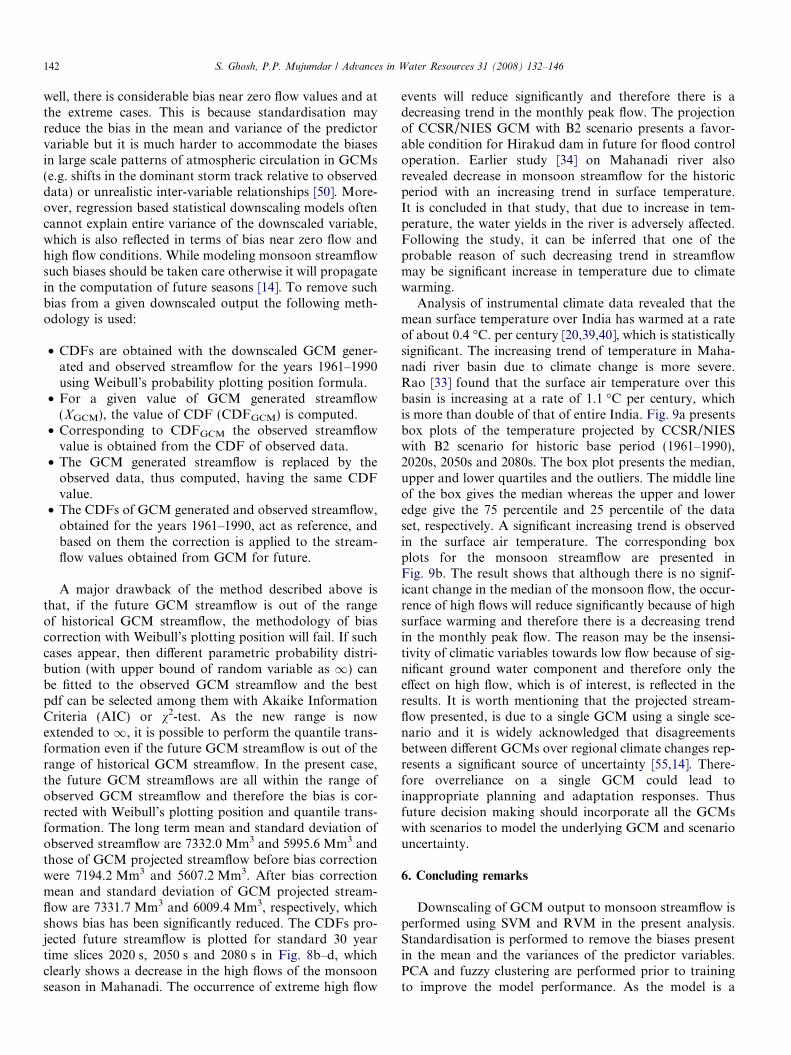
Analysis of instrumental climate data revealed that themean surface temperature over India has warmed at a rateof about 0.4 �C. per century [20,39,40], which is statisticallysignificant. The increasing trend of temperature in Maha-nadi river basin due to climate change is more severe.Rao [33] found that the surface air temperature over thisbasin is increasing at a rate of 1.1 �C per century, whichis more than double of that of entire India. Fig. 9a presentsbox plots of the temperature projected by CCSR/NIESwith B2 scenario for historic base period (1961–1990),2020s, 2050s and 2080s. The box plot presents the median,upper and lower quartiles and the outliers. The middle lineof the box gives the median whereas the upper and loweredge give the 75 percentile and 25 percentile of the dataset, respectively. A significant increasing trend is observedin the surface air temperature. The corresponding boxplots for the monsoon streamflow are presented inFig. 9b. The result shows that although there is no signif-icant change in the median of the monsoon flow, the occur-rence of high flows will reduce significantly because of highsurface warming and therefore there is a decreasing trendin the monthly peak flow. The reason may be the insensi-tivity of climatic variables towards low flow because of sig-nificant ground water component and therefore only theeffect on high flow, which is of interest, is reflected in theresults. It is worth mentioning that the projected stream-flow presented, is due to a single GCM using a single sce-nario and it is widely acknowledged that disagreementsbetween different GCMs over regional climate changes rep-resents a significant source of uncertainty [55,14]. There-fore overreliance on a single GCM could lead toinappropriate planning and adaptation responses. Thusfuture decision making should incorporate all the GCMswith scenarios to model the underlying GCM and scenariouncertainty.

6. Concluding remarks

Downscaling of GCM output to monsoon streamflow isperformed using SVM and RVM in the present analysis.Standardisation is performed to remove the biases presentin the mean and the variances of the predictor variables.PCA and fuzzy clustering are performed prior to trainingto improve the model performance. As the model is a

Fig. 9. (a) Box plot of projected temperature of the case-study area by CCSR/NIES GCM with B2 Scenario and (b) box plot of downscaled streamflowfrom CCSR/NIES GCM output with B2 Scenario.

S. Ghosh, P.P. Mujumdar / Advances in Water Resources 31 (2008) 132–146 143

combination of classification and regression, it can be cat-egorized into a hybrid model of weather typing and trans-fer function. It has been observed that RVM not onlyinvolves probabilistic reasoning but also outperformsSVM for regression based statistical downscaling in termsof goodness of fit. RVM involves fewer number of relevantvectors and the chance of overfitting is less than that ofSVM. The model developed in the present study is capableof producing a satisfactory value of goodness of fit interms of R value and Nash–Sutcliffe coefficient. However,from Fig. 7 it is found that even RVM is not able to mimicthe extreme streamflow observed in the record. Possiblythis could be because regression based statistical downscal-ing models often cannot explain entire variance of thedownscaled variable [54]. Bias resulting from the drawbackis corrected at the end of downscaling. The GCM CCSR/NIES with B2 scenario projects a decreasing trend infuture monsoon streamflow of Mahanadi. In Rao [34], adecreasing trend in the streamflow of Mahandi River withan increasing trend in surface temperature is observed, andit is concluded in that study that due to increase in temper-ature, the water yields in the river is adversely affected.Following the study, it can be inferred that one of the pos-sible reasons for such a decrease in Mahanadi Riverstreamflow may be increase in surface temperature. Sucha decrease in streamflow may cause a critical situationfor Hirakud dam in meeting the future irrigation andpower demand. The methodology developed can be used

to project the streamflow for other GCMs and scenariosalso and there is a possibility of mismatch in the projec-tions resulting GCM and scenario uncertainty. Modelingof such uncertainty is necessary for future decision mak-ing. The methodology presented, does not limit its useful-ness only for modeling streamflow. It is adaptable and canbe used to model any other hydrologic variable, viz. pre-cipitation, evaporation, etc. to assess the impact of climatechange on hydrology.

Appendix 1. Support vector regression

The basic concept of SV regression is discussed in thepresent section first with a linear model and then it isextended to a nonlinear model using Kernels. Given atraining data fðx1; y1Þ; . . . ; ðxl; ylÞ;X 2 Rn; Y 2 Rg, the SVregression equation can be given by [37]

f ðxÞ ¼ hw; xi þ b; w 2 X ; b 2 R ð20Þ

where, hÆ, Æi denoted the dot product in X. The objective ofSVM regression is to find the function f(x) with minimumvalue of loss function and at the same time is as flat as pos-sible [38]. Flatness mathematically denotes the smaller va-lue of w and one way to ensure this is to minimize thenorm, i.e. kwk2 = hw, wi. Thus the model can be expressedas the following convex optimization problem.

144 S. Ghosh, P.P. Mujumdar / Advances in Water Resources 31 (2008) 132–146

Minimize1

2kwk2 þ C

Xl

i

n�i þXl

i¼1

ni

!ð21Þ

subject to yi � hw; xi � b 6 eþ ni ð22Þhw; xi þ b� yi 6 eþ n�i ð23Þni; n

�i P 0 ð24Þ

where C is a pre-specified value which determines the trade-off between the flatness of f(x) and the amount up to whichdeviations larger than e is tolerated (ni and n�i ), which cor-respond to e-insensitive loss function as presented in Eq.(6). The optimization model presented in Eqs. (21)–(24)can be solved using Lagrange multipliers. A dual set ofvariables are introduced to construct the Lagrange func-tion, which is given below:

L ¼ 1

2kwk2 þ C

Xl

i¼1

n�i þXl

i¼1

ni

!�Xl

i¼1

ðgini þ g�i n�i Þ

�Xl

i¼1

aiðeþ ni � yi þ hw; xi þ bÞ

�Xl

i¼1

a�i ðeþ n�i þ yi � hw; xi � bÞ ð25Þ

where L is the Lagrangian and gi; g�i ; ai; a�i are Lagrangian

multipliers satisfying the positivity constraints.

gi; g�i ; ai; a

�i P 0 ð26Þ

From the saddle point condition, the partial derivatives ofL with respect to the primal variables ðw; b; ni; n

�i Þ have to

vanish for optimality:

oLob¼Xl

i¼1

ða�i � aiÞ ¼ 0 ð27Þ

oLow¼ w�

Xl

i¼1

ðai � a�i Þxi ¼ 0 ð28Þ

oL

onð�Þi

¼ C � að�Þi � gð�Þi ¼ 0 ð29Þ

where nð�Þi ; að�Þi ; gð�Þi refer to ni and n�i ; ai and a�i ; gi and g�irespectively.

Substituting Eqs. (27)–(29) in Eq. (25) the followingdual optimization problem is formulated.

Maximize � 1

2

Xl

i;j¼1

ðai � a�i Þðaj � a�j Þhxi; xji � eXl

i¼1

ðai þ a�i Þ

þXl

i¼1

yiðai � a�i Þ ð30Þ

subject toXl

i¼1

ðai � a�i Þ ¼ 0 ð31Þ

ai; a�i 2 ½0;C�: ð32Þ

Eq. (28) can be re-written as

w ¼Xl

i¼1

ðai � a�i Þxi ð33Þ

and, thus from Eq. (20):

f ðxÞ ¼Xl

i¼1

ðai � a�i Þhxi; xi þ b ð34Þ

This is called the Support Vector Expansion for linearmodel which is used in SV regression. b can be computedby using Karush Kuhn Tucker (KKT) condition [38].

For most of the hydrologic analysis linear regression isnot appropriate and thus a nonlinear mapping using kernelK is used to map the data into a higher dimensional featurespace, where, with the kernel, linear analysis is performed.Using the kernel, the regression equation (Eq. (34)) can bemodified to (Eq. (5))

Appendix 2. Kernel functions

Kernel functions are used in SVM for nonlinear map-ping of the original data or input into a high dimensionalfeature space. Kernel function used in a SVM should fol-low Mercer’s theorem, according to which it can be writtenthat:Z

X�XKðx; x0Þf ðxÞf ðx0Þdxdx0 P 0 8f 2 L2ðX Þ ð35Þ

Some of the valid kernel functions satisfying the abovementioned condition are given below.

A. Linear kernel: The linear kernels are the simplest ker-nels used in SVM for linear regression. They can be givenbyHomogeneous kernel:

Kðx; x0Þ ¼ hx; x0i ð36ÞNon-homogeneous kernel:

Kðx; x0Þ ¼ ðhx; x0i þ 1Þ ð37ÞThe performance of SVM with linear kernel function,being similar to that of linear regression, is not capableof modeling complicated and nonlinear relationship be-tween climatological variables and streamflow and there-fore such kernels are not used in the present study.

B. Gaussian Radial Basis Function: Radial Basis Func-tions (RBFs) have received significant attention, most com-monly with Gaussian form,

Kðx; x0Þ ¼ exp �kx� x0k2

2r2

!ð38Þ

where r is the width of Gaussian RBF kernel, giving anidea about the smoothness of the derived function. A largekernel width acts as a low-pass filter in frequency domain,attenuating higher order frequencies and thus resulting in asmooth function. Alternatively, RBF kernel with small ker-nel width retains most of the higher order frequencies lead-ing to an approximation of a complex function by learningmachine [38].

C. Laplacian or Exponential Radial Basis Function:Laplacian or Exponential RBF of the form,

S. Ghosh, P.P. Mujumdar / Advances in Water Resources 31 (2008) 132–146 145

Kðx; x0Þ ¼ exp �kx� x0k2r2

� �ð39Þ

produces a piecewise linear solution which can be attractivewhen discontinuities are acceptable.

D. Heavy tailed or Sublinear Radial Basis Function:Heavy tailed RBFs or Sublinear RBFs are introduced byChapelle et al. [10] which sometimes outperform traditionalGaussian or RBFs [10]. They can be given by:

Kðx; x0Þ ¼ exp �kx� x0k0:5

2r2

!ð40Þ

It is worth mentioning that a generalized RBF can be givenby

Kðx; x0Þ ¼ exp �kxa � x0akb

2r2

!ð41Þ

and it will satisfy Mercer’s condition if and only if0 6 b 6 2. The choice of a has no impact on Mercer’scondition.

References

[1] ASCE Task Committee on definition of Criteria for Evaluation ofWatershed Models of the Watershed Management Committee,Irrigation and Drainage Division. Criteria for Evaluation ofWatershed Models. J Irrig Drain Eng 1993;119(3):429–442.

[2] Bardossy A, Plate EJ. Modeling daily rainfall using a semi-Markovrepresentation of circulation pattern occurrence. J Hydrol1991;122:33–47.

[3] Bardossy A, Duckstein L, Bogardi I. Fuzzy rule-based classificationof atmospheric circulation patterns. Int J Climatol 1995;15:1087–97.

[5] Bates BC, Charles SP, Hughes JP. Stochastic downscaling ofnumerical climate model simulations. Environ Model Software1998;13:325–31.

[6] Berger JO. Statistical decision theory and Bayesian analysis. 2nded. New York: Springer; 1985.

[7] Brown BG, Katz RW. Regional analysis of temperature extremes:spatial analog for climate change? J Clim 1995;8:108119.

[8] Burges CJC, Scholkopf B. Improving the accuracy and speed ofsupport vector machines. In: Mozer MC, Jordan MI, Petsche T,editors. Advances in neural information processing systems, vol.9. MIT Press; 1997. p. 375–81.

[9] Cannon AJ, Whitfield PH. Downscaling recent streamflow conditionsin British Columbia, Canada using ensemble neural network models.J Hydrol 2002;259:136–51.

[10] Chapelle O, Haffner P, Vapnik VN. Support vector machines forhistogram-based image classification. IEEE Trans Neural Networks1999;10(5):1055–64.

[11] Crane RG, Hewitson BC. Doubled CO2 precipitation changes for theSusquehanna Basin: down-scaling from the genesis general circulationmodel. Int J Climatol 1998;18:6576.

[12] Dibike YB, Velickov S, Solomatine D, Abbott MB. Model inductionwith support vector machines: introduction and applications. JComput Civil Eng, ASCE 2001;15(3):208–16.

[13] Ghosh S, Mujumdar PP. Future rainfall scenario over Orissa withGCM projections by statistical downscaling. Curr Sci2006;90(3):396–404.

[14] Ghosh S, Mujumdar PP. Nonparametric methods for modeling GCMand scenario uncertainty in drought assessment. Water Resour Res[in print MS No. 2006WR005351].

[15] Govindaraju RS. Bayesian learning and relevance vector machinesfor hydrologic applications. In: Proceedings of the second Indian

international conference on artificial intelligence (IICAI-05), Pune,India; 2005.

[16] Guler C, Thyne GD. Delineation of hydrochemical facies distributionin a regional groundwater system by means of fuzzy c-meansclustering. Water Resour Res 2004;40:W12503. doi:10.1029/2004WR003299.

[17] Gunn SR, Brown M, Bossley KM. Network performance assessmentfor neuro fuzzy data modelling. In: Liu X, Cohen P, Berthold M,editors. Intelligent data analysis. Lecture notes in computer science,vol. 1208. Berlin Heidelberg: Springer-Verlag; 1997. p. 313–23.

[18] Hewitson BC, Crane RG. Large-scale atmospheric controls on localprecipitation in tropical Mexico. Geophys Res Lett1992;19(18):18351838.

[19] Hewitson BC, Crane RG. Climate downscaling: techniques andapplication. Climate Res 1996;7:85–95.

[20] Hingane LS, Rupakumar K, Ramanamurthy BV. Long-term trendsof surface air temperature in india. J Climatol 1985;5:521–8.

[21] Hughes JP, Lettenmaier DP, Guttorp P. A stochastic approach forassessing the effect of changes in synoptic circulation patterns onGauge precipitation. Water Resour Res 1993;29(10):3303–15.

[22] Hughes JP, Guttorp P. A class of stochastic models for relatingsynoptic atmospheric patterns to regional hydrologic phenomena.Water Resour Res 1994;30(5):1535–46.

[23] Hughes JP, Guttorp P, Charles SP. A non-homogeneous hiddenMarkov model for precipitation occurrence. Appl Statist1999;48(1):15–30.

[24] Jones PD, Murphy JM, Noguer M. Simulation of climate changeover europe using a nested regional-climate model, I: assessment ofcontrol climate, including sensitivity to location of lateral boundaries.QJR Meteorol Soc 1995;121:1413–49.

[25] Kalnay E, Kanamitsu M, Kistler R, Collins W, Deaven D, Gandin L,et al. The NCEP/NCAR 40-year reanalysis project. Bull AmMeteorolog Soc 1996;77(3):437471.

[26] Katz RW, Parlange MB. Mixtures of stochastic processes: applica-tions to statistical downscaling. Clim Res 1996;7:185–93.

[27] Khalil A, McKee M, Kemblowski M, Asefa T. Sparse Bayesianlearning machine for real-time management of reservoir releases.Water Resour Res 2005;41:W11401. doi:10.1029/2004WR003891.

[28] Khalil AF, McKee M, Kemblowski M, Asefa T, Bastidas L.Multiobjective analysis of chaotic dynamic systems with sparselearning machines. Adv Water Resour 2006;29(1):72–88.

[29] MacKay D. Information theory, inference, and learning algo-rithms. Cambridge University Press; 2003.

[30] Mehrotra R, Sharma A. A nonparametric nonhomogeneous hiddenMarkov model for downscaling of multi-site daily rainfall occur-rences. J Geophys Res – Atmos 2005;110(D16):16108.

[31] Murphy JM. An evaluation of statistical and dynamical techniquesfor downscaling local climate. J Clim 1999;12:2256–84.

[32] Nash JE, Sutcliffe JV. River flow forecasting through conceptualmodels, Part-1: a discussion of principles. J Hydrol 1970;10:282290.

[33] Rao PG, Kumar KK. Climatic shifts over Mahanadi River Basin.Curr Sci 1992;63:192–6.

[34] Rao PG. Effect of climate change on streamflows in the MahanadiRiver Basin, India. Water Int 1995;20:205–12.

[35] Ross TJ. Fuzzy logic with engineering applications. McGrawhillInternational Edition; 1997. p. 379–96.

[36] Roubens M. Fuzzy clustering algorithms and their cluster validity.Eur J Oper Res 1982;10:294–301.

[37] Smola AJ. Regression estimation with support vector learningmachines. Munchen, Germany: Technische Universitat Munchen;1996.

[38] Smola AJ, Schoelkopf B. A tutorial on support vector regression,NeuroCOLT2. Technical Report NC2-TR-1998-030, Royal Hollo-way College, University of London, UK; 1998.

[39] Srivastava HN, Devan BN, Dixit SK, Prakasarao GS, Singh SS, RaoRK. Decadal trends in climate over India. Mausam 1992;43:7–20.

[40] Thapliyal V, Kulshrestha UC. Climate changes and trends over India.Mausam 1991;42:333–8.

146 S. Ghosh, P.P. Mujumdar / Advances in Water Resources 31 (2008) 132–146

[41] Tripathi S, Srinivas VV. Downscaling of general circulation models toassess the impact of climate change on rainfall of India. In:Proceedings of international conference on hydrological perspectivesfor sustainable development (HYPESD – 2005), 23–25 February, IITRoorkee, India; 2005, p. 509–17.

[42] Tripathi S, Srinivas VV, Nanjundiah RS. Downscaling of precipita-tion for climate change scenarios: a support vector machineapproach. J Hydrol 2006;330:621–40.

[43] Suykens JAK. Nonlinear modelling and support vector machines. In:Proceedings of IEEE instrumentation and measurement technologyconference, Budapest, Hungary; 2001. p. 287–94.

[44] Tipping ME. Sparse Bayesian learning and the relevance vectormachine. J Mach Learn Res 2001;1:211–44.

[45] Trigo RM, Palutikof JP. Simulation of daily temperatures for climatechange scenarios over Portugal: a neural network model approach.Clim Res 1999;13:45–59.

[46] Vapnik VN. The nature of statistical learning theory. NewYork: Springer Verlag; 1995.

[47] Vapnik VN. Statistical learning theory. New York: Wiley; 1998.[48] Wahba G. A comparison of GCV and GML for choosing the

smoothing parameter in the generalized spline-smoothing problem.Ann Stat 1985;4:1378402.

[49] Wetterhall F, Halldin S, Xu C. Statistical precipitation downscalingin Central Sweden with the analogue method. J Hydrol2005;306:174–90.

[50] Wilby RL, Dawson CW. Using SDSM version 3.1 A decision supporttool for the assessment of regional climate change impacts, UserManual; 2004.

[51] Wilby RL, Wigley TML, Conway D, Jones PD, Hewitson BC,Main J, et al. Statistical downscaling of general circulation modeloutput: a comparison of methods. Water Resour Res 1998;34:2995–3008.

[52] Wilby RL, Hay LE, Leavesly GH. A comparison of downscaled andraw GCM output: implications for climate change scenarios in theSan Juan River Basin, Colorado. J Hydrol 1999;225:67–91.

[53] Wilby RL, Dawson CW, Barrow EM. SDSM – a decision supporttool for the assessment of regional climate change impacts. EnvironModell Softw 2002;17(2):147–59.

[54] Wilby RL, Charles SP, Zorita E, Timbal B, Whetton P, Mearns LO.The guidelines for use of climate scenarios developed from statisticaldownscaling methods. Supporting material of the IntergovernmentalPanel on Climate Change (IPCC), prepared on behalf of Task Groupon Data and Scenario Support for Impacts and Climate Analysis(TGICA). <http://ipccddc.cru.uea.ac.uk/guidelines/StatDown_Guide.pdf>; 2004.

[55] Wilby RL, Harris I. A framework for assessing uncertainties inclimate change impacts: low-flow scenarios for the River Thames,UK. Water Resour Res 2006;42:W02419. doi:10.1029/2005WR004065.

[56] Wilks DS. Multisite downscaling of daily precipitation with astochastic weather generator. Clim Res 1999;11:125–36.

[57] Willmott CJ, Rowe CM, Philpot WD. Small-scale climate map: asensitivity analysis of some common assumptions associated with thegrid-point interpolation and contouring. Am Cartographer1985;12:5–16.