Embed Size (px)
Citation preview

ANKUR SINGH March, 2013
ITC SUPERVISOR IIRS SUPERVISORS
Dr. N.A.S. Hamm Ms. Vandita Srivastava
Downscaling leaf area index using downscaling cokriging on optical remotely sensed data


Thesis submitted to the Faculty of Geo-information
Science and Earth Observation of the University of Twente
in partial fulfilment of the requirements for the degree of
Master of Science in Geo-information Science and Earth
Observation.
Specialization: Geoinformatics
ITC SUPERVISOR IIRS SUPERVISORS
Dr. N.A.S. Hamm Ms. Vandita Srivastava
THESIS ASSESSMENT BOARD:
Chairperson : Prof.dr.ir. M.G. Vosselman
ITC Theme Leader : Prof. dr.ir. A. Stein.
First Supervisor (IIRS) : Ms. Vandita Srivastava
Second Supervisor (ITC) : Dr. N.A.S. Hamm
External Examiner : Prof C.Jeganathan(BIT,Ranchi)
Downscaling leaf area index using downscaling cokriging on optical remotely sensed data
ANKUR SINGH
Enschede, the Netherlands [March, 2013]

DISCLAIMER
This document describes work undertaken as part of a programme of study at the Faculty of
Geo-Information Science and Earth Observation (ITC), the University of Twente, The
Netherlands. All views and opinions expressed therein remain the sole responsibility of the
author, and do not necessarily represent those of the Faculty.

“The keys to patience are acceptance and faith. Accept things as they
are, and look realistically at the world around you. Have faith in
yourself and in the direction you have chosen.”
By: Ralph Marston
-
Dedicated to my parents........


I
ABSTRACT
In the field of remote sensing, scaling of data has become more practicing in different disciplines.
Downscaling of data bring revolution for the usage of coarse spatial resolution data products.
The data products were downscaled to desired fine resolution according to the usage. In this
study LAI (leaf area index) is downscaled by using cokriging technique. The main aim of this
research is to explore downscaling cokriging technique by studying the effect of resampling and
point spread function (PSF).
MODIS LAI product at 1000 m spatial resolution is used as primary variable and MODIS NDVI
at 250 m is used as covariable to downscale LAI at 250 m. Cokriging is used as the technique for
downscaling. The first step for downscaling cokriging involves the calculating of sample
variogram and cross-variogram. To calculate cross-variogram both the variable LAI and NDVI
should be on same scale. To bring MODIS LAI at 250 m it is resample at 250 m and cross-
variogram is calculated between resample LAI and original NDVI at constant cut-off of 6000 m
and bin of 15 and variogram and cross-variogram is modelled at common range of 3817.4 m
using exponential model. To select optimal resampling from different resampling techniques
(nearest neighbour, bilinear interpolation, cubic convolution and trivial method) variogram
analysis has been executed. It was found that variance in trivial resampling was highest (sill =
3.78) which shows high spatial dependence. Trivial resampling is also selected for resampling
because it resample’s pixel size with original pixel values. Gaussian and uniform PSF are used to
study the effect of PSF on variogram. Standard deviation and were parameterized by
experimenting with different value of standard deviation. and were parameterized at 250 m
for MODIS LAI at resolution 1000 m and 122.5 m for MODIS NDVI at resolution 250m.
Further, point support variogram and cross-variogram were estimated to see the effect of both
(uniform and Gaussian) PSF by keeping rest of the parameter same and using nested exponential
model. It was found that for LAI 1000 m using uniform PSF sill was 2.85 for the range 3040.5m
which is more than that by using Gaussian PSF (2.06 for range 3857.0 m). It was found that
variance is high using uniform PSF for LAI at 1000 m because distance from the pixel or the
mean is more. It was observed that for NDVI at 250 m there is very less difference is observed
by estimated point support variogram which was not observed by modelling of point support
variogram in and variance for uniform PSF was found higher than by using Gaussian PSF. There
was no change observed for the cross-variogram because PSF does not have much effect for
different bands on same support. Due to above change the effect was also observed on the
centre of downscaling cokriging weights. By using uniform PSF centre of the weight was high
than that by using Gaussian PSF. There is change observed in the downscaled cokriging image.
The downscaled image for Gaussian PSF was found smoother than that of uniform PSF. The
standard deviation in downscaled image for uniform PSF (1.73) was found more than that of
Gaussian PSF (1.69) which shows that variance is high for the uniform PSF than that of Gaussian
PSF.
Keywords: Downscaling, cokriging, MODIS LAI, MODIS NDVI, resampling, Point spread
function (PSF), uniform PSF, Gaussian PSF, variogram

II

III
ACKNOWLEDGEMENTS
This thesis duration is one of the most learning phases of my life. The modules and pilot projects
during my M.Sc. course became the base of this research. I would not have finished this research
successfully without the help, support and moral boosting from many individuals.
Firstly and most importantly I would like to show my gratitude toward my supervisors Ms.
Vandita Srivastava and Dr. Nicholas Hamm. Their expert guidance, valuable suggestions,
constructive criticism and encouragement act as a four pillar of my thesis. Their critical and
logical thinking helped me to complete this thesis successfully. Thanks to you both.
I would like to show honour to Prof. Alfred Stein and Dr. Nicholas Hamm for givng a valueable
lecture in ITC on geostatistics which make my interest in the subject and also providing all small
details on formalizing MSc thesis on their last visit to IIRS.
I would also like to acknowledge Mr. Prasun Kumar Gupta GID, IIRS who had spent his
valuable time to help me out with the FORTRAN software issues.
I would also like to thank IIRS-ITC joint education program for allowing me to get into M.Sc.
course. This course taught me a lot academically and also helped me to explore the culture of The
Netherlands. I am also thankful to ITC for providing access to excellent facilities like electronic
library, blackboard, webmail, softwares etc.
I would also like to give special thanks to Dr. Y.V.N.Krishna Murthy, Director IIRS, Mr. P.L.N.
Raju, Group head (RS and GIS) IIRS and Dr.S.K.Srivastava, Head Geo Informatics Division,
IIRS for providing wonderful infrastructure which has helped me in finishing this research
successfully and taking care of all the requirements. I am also thankful to IIRS library and CMA
department for providing me facilities and resources.
I specially thank Priyanka Arya, for her keen support to keep my moral high and helped to stay
focused on my project. I am also thankful to my roommate and friend Jayson for his outstanding
support and for many fruitful discussions which helped in expanding my knowledge.
I would also like to thanks all my friends in IIRS and outside IIRS for their support and for the
wonderful time spent here.
Last but not the least, without the support of my family and almighty god I would not have finished this project. Since, they were not present here with me but their blessings and support was always to my take care.

IV
TABLE OF CONTENTS
List of Figures............................................................................................................................................................VII
List of Tables............................................................................................................................................................VIII
1. INTRODUCTION ............................................................................................................ 1
1.1. Background ....................................................................................................................................................... 1 1.2. Research Identifications ................................................................................................................................. 3 1.2.1. Research Objectives.................................................................................................................................... 3
1.2.2. Research Questions .................................................................................................................................... 3
1.3. Innovation aimed at ........................................................................................................................................ 3 1.4. Thesis Strucure ................................................................................................................................................. 3
2. CONCEPTUAL AND THEORETICAL BACKGROUND .......................................... 5
2.1. Terrestrial ecosystem ....................................................................................................................................... 5 2.2. Biophysical variables ....................................................................................................................................... 6 2.2.1. Leaf Area Index ........................................................................................................................................... 6
2.3. Vegetation Indices ........................................................................................................................................... 7 2.4. LAI-NDVI relationship .................................................................................................................................. 7 2.5. Resampling........................................................................................................................................................ 8 2.6. Downscaling ................................................................................................................................................... 10 2.6.1. Introduction ............................................................................................................................................... 10
2.6.2. Downscaling Techniques ......................................................................................................................... 11
2.7. Point spread function .................................................................................................................................... 12
3. STUDY AREA AND DATA DESCRIPTION .............................................................. 14
3.1. Study Area ....................................................................................................................................................... 14 3.2. Data used ........................................................................................................................................................ 16 3.2.1. Satellite data ............................................................................................................................................... 16
4. Materials and METHODOLOGY .................................................................................. 18
4.1. Estimating correlation between LAI, NDVI, reflectance band (red, NIR) ......................................... 18 4.2. Resampling LAI from 1000 m to 250 m for calculating sample variogram ......................................... 19 4.3. Modelling semi-variogram and cross-variogram for convolution and de-convolution using uniform PSF and Gaussian PSF. .............................................................................................................................................. 19 4.4. Cokriging system to estimate the downscaling cokriging weights and to obtain the downscaled image. 22 4.5. Comparison of downscaled images obtained using uniform and Gaussian PSF ................................ 23 4.6. Summary of the method ............................................................................................................................... 24 4.7. Software used ................................................................................................................................................. 27
5. RESULTS.......................................................................................................................... 28
5.1. Correlation of LAI with NDVI, NIR and Red bands from optical image ......................................... 28 5.2. Impact of resampling on the variogram..................................................................................................... 28 5.3. Impact of PSF on variogram ....................................................................................................................... 31 5.4. Impact of PSF on downscaling cokriging .................................................................................................. 34 5.4.1. Comparison between downscaled image using uniform PSF and Gaussian PSF .......................... 39
5.5. Summary of the Results ................................................................................................................................ 40

V
6. DISCUSSION .................................................................................................................. 41
6.1. Correlation of LAI with NDVI, NIR and Red bands from optical image .......................................... 41 6.2. Impact of resampling on the variogram and cross variogram ............................................................... 41 6.3. Impact of PSF on variogram and cross-variogram ................................................................................. 42 6.4. Impact of PSF on downscaling cokriging ................................................................................................. 42
7. CONCLUSION AND RECOMMENDATIONS ......................................................... 44
7.1. Conclusions .................................................................................................................................................... 44 7.2. Recommendation .......................................................................................................................................... 45

VI
LIST OF FIGURES
Figure 2-1 : Terrestrial ecosystem (Ollinger, 2003) .................................................................................. 5
Figure 2-2 : Nearest Neighbour resampling (Studley and Weber, 2010) .............................................. 9
Figure 2-3 : Bilinear Interpolation resampling (Studley and Weber, 2010) .......................................... 9
Figure 2-4 : Cubic convolution resampling (Studley and Weber, 2010) ............................................ 10
Figure 2-5 : Uniform PSF (Pardo-Iguzquiza and Atkinson, 2007)..................................................... 12
Figure 2-6 : Gaussian PSF (Pardo-Iguzquiza and Atkinson, 2007) .................................................... 12
Figure 3-1 : Study area ............................................................................................................................... 15
Figure 3-2 : The tiles covering MODIS product (Myneni et al., 2003).............................................. 16
Figure 4-1 : Estimation of correlation between LAI and NDVI, red reflectance. ........................... 18
Figure 4-2 : Fusion of coarser and finer resolution image by applying cokriging weights to obtain
downscaled MODIS LAI image at 250 m spatial resolution ...................................................... 23
Figure 4-3 : Resampling by using trivial method. .................................................................................. 24
Figure 4-4 : Method adopted in this study ............................................................................................. 26
Figure 5-1 : Cross-variogram between MODIS NDVI 250 m and resampled LAI 250 m using
NN resampling ................................................................................................................................... 29
Figure 5-2 : Cross-variogram between MODIS NDVI 250 m and resample LAI 250 m using BI
resampling ........................................................................................................................................... 29
Figure 5-3 : Cross-variogram between MODIS NDVI 250 m and resample LAI 250 m using CC
resampling ........................................................................................................................................... 30
Figure 5-4 : Cross-variogram between MODIS NDVI 250 m and resample LAI 250 m using
trivial resampling ................................................................................................................................ 31
Figure 5-5 : (a) Estimated point support variogram for MODIS LAI from 1000 m for uniform
PSF (b) Estimated point support variogram for MODIS LAI from 1000 m for Gaussian PSF
.............................................................................................................................................................. 32
Figure 5-6 : (a) Estimated point support variogram for MODIS NDVI from 250 m for uniform
PSF (b) Estimated point support variogram for MODIS NDVI from 250 m for Gaussian
PSF ....................................................................................................................................................... 32
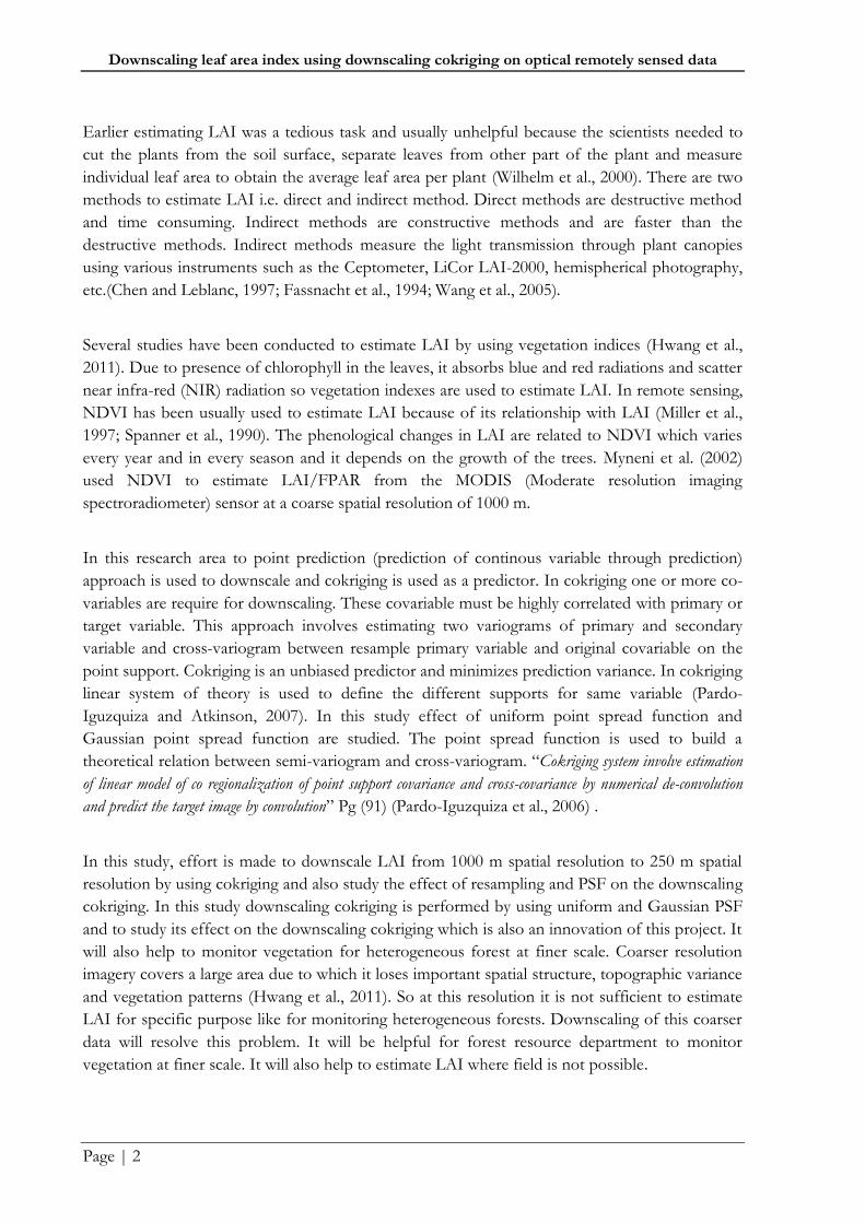
Figure 5-7 : (a) Estimated point support cross-variogram between MODIS NDVI 250 m and
resample LAI from 250 m for uniform PSF(b) Estimated point support cross-variogram
between MODIS NDVI 250 m and resampled LAI from 250 m for uniform PSF ............... 33
Figure 5-8 : Downscaled image of MODIS LAI at 250 m using uniform PSF................................ 37
Figure 5-9 : Downscaled image of MODIS LAI at 250 m using Gaussian PSF .............................. 37
Figure 5-10 : (a) Histogram of LAI showing occurrence of downscaled MODIS LAI at 250 m
using uniform PSF (b) Histogram of LAI showing occurrence of downscaled MODIS LAI
at 250 m using Gaussian PSF ........................................................................................................... 38
Figure 5-11 : (a) Boxplot of LAI showing distribution of downscaled MODIS LAI at 250 m using
uniform PSF(b) Boxplot of LAI showing distribution of downscaled MODIS LAI at 250 m
using Gaussian PSF ........................................................................................................................... 38

VII
LIST OF TABLES
Table 4.1: Description of software used ................................................................................................. 27
Table 5.1 : Correlation of LAI with the variables NDVI, NIR and Red reflectance ....................... 28
Table 5.2 : Fitting of model to cross-variogram between MODIS NDVI 250 m and resample LAI
250 m for NN resampling ................................................................................................................ 29
Table 5.3 : Fitting of model to cross-variogram between MODIS NDVI 250 m and resample LAI
250 m for BI resampling ................................................................................................................... 30
Table 5.4 : Fitting of model to cross-variogram between MODIS NDVI 250 m and resample LAI
250 m for CC resampling .................................................................................................................. 30
Table 5.5 : Fitting of model to cross-variogram between MODIS NDVI 250 m and resample LAI
250 m for trivial resampling.............................................................................................................. 31
Table 5.6 : Modelled point support variogram for estimated point support variogram for MODIS
LAI 1000 m ......................................................................................................................................... 33
Table 5.7 : Modelled point support variogram for estimated point support variogram for MODIS
NDVI 250 m....................................................................................................................................... 33
Table 5.8 : Modelled point support cross-variogram for estimated point support cross-variogram
between MODIS NDVI 250 m and LAI resample at 250 m ...................................................... 33
Table 5.9 :(a) Example of Cokriging weights of 3 x 3 window which act as high pass filter for
coarser resolution image (MODIS LAI 1000 m) obtained by using uniform PSF (b) Example
of Cokriging weights of 4 x 4 window which act as low pass filter for finer resolution image
(MODIS NDVI 250 m) obtained by using uniform PSF ............................................................ 35
Table 5.10 : (a) Example of Cokriging weights of 3 x 3 window which act as high pass filter for
coarser resolution image (MODIS LAI 1000 m) obtained by using Gaussian PSF: (b)
Example of Cokriging weights of 4 x 4 window which act as low pass filter for finer
resolution image (MODIS NDVI 250 m) obtained by using Gaussian PSF ............................ 36
Table 5.11 : Spatial distribution of downscaled LAI value obtained by using uniform and
Gaussian PSF ...................................................................................................................................... 39
Table 5.12: Auto-covariance between downscaled image using uniform and Gaussian PSF ......... 40


Downscaling leaf area index using downscaling cokriging on optical remotely sensed data
Page | 1
1. INTRODUCTION
1.1. Background
In the field of remote sensing, scaling of data has become more practicing. According to the
application, the resolution of the data can be changed either by upscaling or downscaling.
Upscaling refers to the practice of converting finer spatial resolution data to coarser spatial
resolution data. For example, ground data are upscaled to match with the pixel of an image
(Atkinson, 2012). Downscaling is when coarser spatial resolution is converted to finer spatial
resolution. These days’ downscaling is of much interest to the researchers for exploration and to
practitioners for implementing the fusion of different data of varying scales. The reason an
optimal pixel size is defined by researchers is due to the issue of scaling (Atkinson and Curran,
1995; Atkinson et al., 1997; Woodcock and Strahler, 1987). The sensor which has the coarse
resolution has a large coverage and high revisit time, which provides ample information more
frequently. For example, MODIS has a spatial resolution of 250 m, 500 m and 1000 m and has a
revisit time of more than 8 days. On the other hand, fine spatial resolution gives more detailed
information with low revisit time. For example ASTER and LANDSAT series satellite has revisit
time of 16 and 18 days.
The advantage of downscaling is to extract the detailed information from coarser resolution at
high temporal resolution. This technique is also cost effective since fine resolution data are
costlier than coarse resolution data. Atkinson (2012) stated that there are two approaches for
downscaling: regression approaches and area to point predictions. In regression approach, finer
spatial resolution is estimated from a coarser spatial resolution. This is done with the help of
covariate as a variable. This approach does not consider support and also does not characterize
pattern of spatial variation while area to point prediction interpolates using both support and also
characterizes the pattern of spatial variation (Atkinson, 2012). In the present study, area to point
prediction is used as technique, leaf area index (LAI) is used as a target or primary variable and
NDVI is used as a covariable for downscaling.
Leaf area index is one of the main variables for characterizing plants’ canopy. Leaf area index
(LAI) is defined as the area of one side of the leaf per unit area of the ground (Myneni et al.,
2002) It is a biophysical variable which influences vegetation photosynthesis, transpiration and
land surface energy (Tian et al., 2002). It is an important variable of ecosystem because most of
the ecosystem models that stimulate carbon and hydrological cycles require LAI as an input
(Gower et al., 1999). Estimating LAI has become easier by using satellite data like MODIS which
has a LAI product of spatial resolution of 1000 m for every 8 days. Much research has been
conducted to estimate LAI for different forest types like coniferous forest, tropical forest,
deciduous forest and broadleaf forest (Asner et al., 2003)
Downscaling leaf area index using downscaling cokriging on optical remotely sensed data
Page | 2
Earlier estimating LAI was a tedious task and usually unhelpful because the scientists needed to
cut the plants from the soil surface, separate leaves from other part of the plant and measure
individual leaf area to obtain the average leaf area per plant (Wilhelm et al., 2000). There are two
methods to estimate LAI i.e. direct and indirect method. Direct methods are destructive method
and time consuming. Indirect methods are constructive methods and are faster than the
destructive methods. Indirect methods measure the light transmission through plant canopies
using various instruments such as the Ceptometer, LiCor LAI-2000, hemispherical photography,
etc.(Chen and Leblanc, 1997; Fassnacht et al., 1994; Wang et al., 2005).
Several studies have been conducted to estimate LAI by using vegetation indices (Hwang et al.,
2011). Due to presence of chlorophyll in the leaves, it absorbs blue and red radiations and scatter
near infra-red (NIR) radiation so vegetation indexes are used to estimate LAI. In remote sensing,
NDVI has been usually used to estimate LAI because of its relationship with LAI (Miller et al.,
1997; Spanner et al., 1990). The phenological changes in LAI are related to NDVI which varies
every year and in every season and it depends on the growth of the trees. Myneni et al. (2002)
used NDVI to estimate LAI/FPAR from the MODIS (Moderate resolution imaging
spectroradiometer) sensor at a coarse spatial resolution of 1000 m.
In this research area to point prediction (prediction of continous variable through prediction)
approach is used to downscale and cokriging is used as a predictor. In cokriging one or more co-
variables are require for downscaling. These covariable must be highly correlated with primary or
target variable. This approach involves estimating two variograms of primary and secondary
variable and cross-variogram between resample primary variable and original covariable on the
point support. Cokriging is an unbiased predictor and minimizes prediction variance. In cokriging
linear system of theory is used to define the different supports for same variable (Pardo-
Iguzquiza and Atkinson, 2007). In this study effect of uniform point spread function and
Gaussian point spread function are studied. The point spread function is used to build a
theoretical relation between semi-variogram and cross-variogram. “Cokriging system involve estimation
of linear model of co regionalization of point support covariance and cross-covariance by numerical de-convolution
and predict the target image by convolution” Pg (91) (Pardo-Iguzquiza et al., 2006) .
In this study, effort is made to downscale LAI from 1000 m spatial resolution to 250 m spatial
resolution by using cokriging and also study the effect of resampling and PSF on the downscaling
cokriging. In this study downscaling cokriging is performed by using uniform and Gaussian PSF
and to study its effect on the downscaling cokriging which is also an innovation of this project. It
will also help to monitor vegetation for heterogeneous forest at finer scale. Coarser resolution
imagery covers a large area due to which it loses important spatial structure, topographic variance
and vegetation patterns (Hwang et al., 2011). So at this resolution it is not sufficient to estimate
LAI for specific purpose like for monitoring heterogeneous forests. Downscaling of this coarser
data will resolve this problem. It will be helpful for forest resource department to monitor
vegetation at finer scale. It will also help to estimate LAI where field is not possible.

Downscaling leaf area index using downscaling cokriging on optical remotely sensed data
Page | 3
1.2. Research Identifications
1.2.1. Research Objectives
The main objective of this research is to study the effect of resampling and PSF on downscaling
cokriging technique for LAI estimation.
Sub-objectives:
1. To downscale LAI using cokriging by covariable.
2. To study the effect of resampling on variogram.
3. To study the effect of PSF on variogram and downscaled LAI image.
1.2.2. Research Questions
To achieve the above objective the following questions need to be answered.
1. What is the suitable covariable and its correlation with LAI?
2. What is the effect of resampling on variogram and cross-variogram?
3. What is the effect of PSF on variogram and cross-variogram?
4. What is the effect of PSF on resultant downscaled image?
1.3. Innovation aimed at
The innovation of this project is to perform downscaling cokriging by using uniform and
Gaussian PSF and also to study the effect of these PSF on downscaling cokriging technique.
1.4. Thesis Strucure
This structure of the thesis describes the whole project and the content related to this research in
chapters:
Chapter 1: Introduction, this section describes general overview about this research work. It
describe the basic idea of topic, motivation for selecting this topic, problem statement, research
objectives, and research questions to carry out this task.
Chapter 2: Theoretical Background and Literature Review, this chapter contains theoretical
background of the study and literature study.
Chapter 3: Study area and data used, this chapter describes selection of study area and description
of the study area. It also contains the description of data used and software used.
Chapter 4: Methodology, this chapter describes complete workflow of the study and description
of each and every steps of methodology.
Chapter 5: Results, this chapter contains results which I obtained using above methodology.

Downscaling leaf area index using downscaling cokriging on optical remotely sensed data
Page | 4
Chapter 6: Discussion, this chapter explain results and also its implications.
Chapter 7: Conclusion and Recommendation, this section describes the answer of the research
questions in conclude form. Some important points are recommended after experience got from
this whole work and recommendation for future work.

Downscaling leaf area index using downscaling cokriging on optical remotely sensed data
Page | 5
2. CONCEPTUAL AND THEORETICAL BACKGROUND
2.1. Terrestrial ecosystem
Terrestrial ecosystem has an essential role in the overall carbon cycle. It is responsible for the
exchange of which brings changes in atmospheric concentration. Terrestrial ecosystem
affects the climate in number of ways that act over extent and duration scales. Forests are the
most resourceful terrestrial ecosystem on Earth, providing essential goods and services upon
which the humanity is very much dependent (Song, 2013). Due to changes in the area and
changes during time in forest ecosystem affect global carbon cycle and also responsible for the
climate change (Goodale et al., 2002). Increase in carbon content in forest ecosystems is a
forewarning to take the most important step against global warming. Satellite remote sensing
provides a unique way to obtain the distributions of LAI over large areas.
Leaf area index (LAI) is generally used to describe the photosynthetic and transpirational surface
of plant canopies. LAI can be defined as the leaf surface area per unit ground area. It is an
important variable in controlling many biological and physical processes. (Running et al., 1999)
LAI is an essential input variable which is used for many climate and ecological models.
Green leaves are good absorbers of solar radiation. Compared with non vegetative surfaces,
absorption in green leaves are more in visible spectrum for photosynthesis and less in near
infrared radiation. Reflectance in red and near infrared wavebands has been used to formulate
various vegetation indices because they indicate all the conditions of the vegetation surface (Qi et
al., 1994). Among the various vegetation indices, NDVI (Wang et al., 2005), is most frequently
used to derive LAI . There have also been several investigations on this relationship between
satellite-derived vegetation indices and LAI for various forest type and species (Spanner et al.,
1990(b); Spanner et al., 1990(a)).
Figure 2-1 : Terrestrial ecosystem (Ollinger, 2003)

Downscaling leaf area index using downscaling cokriging on optical remotely sensed data
Page | 6
2.2. Biophysical variables 2.2.1. Leaf Area Index
Leaf area index is most important biophysical variable of ecosystem models (Propastin and
Erasmi, 2010). Spatial distribution of LAI on Earth’s surface is helpful in understanding various
biophysical processes within a terrestrial ecosystem, such as photosynthesis, respiration,
transpiration, carbon and nutrient cycle and rainfall interception ((Fassnacht et al., 1997; Hu et al.,
2003; Miller et al., 1997); Peng et al. (2003)). LAI describes physiological, climatological and
biogeochemical conditions due to vegetation conditions (Asner et al., 1998). Asner et al. (2003)
stated that LAI can be estimated, modelled, and analysed at different resolution scales (from a
small tree to whole forest and from whole forest to whole continents level because it has no
unit). LAI is strongly correlated to vegetation species, growing stage, seasonal variance, field
conditions and management practices.
To estimate LAI many methods were used from several years. Jonckheere et al. (2004) describes
different methods to estimate LAI which are categorized into 2 categories i.e.:
Direct method
Indirect method
The accuracy of direct method is more than that of indirect method because leaves are cut and
measured manually. The main disadvantage of this method is that it is time consuming and for
large scale it is not feasible. There is more error in this method because of repeating
measurements. This method is further divided into sub categories i.e.:
Harvesting and non-harvesting methods(which is well explained in (Jonckheere et
al., 2004))
Leaf area determination techniques (which is well explained in (Jonckheere et al.,
2004))
Indirect methods are faster than direct method. In this method leaf area can be determined by
another variable. Jonckheere et al. (2004) stated that in field, indirect method is subdivided into
two categories i.e.
Estimating LAI from indirect contact.
Inclined point quadrant
Allometric method
Estimating LAI from indirect non-contact (optical method).
Digital plant canopy imager
Plant canopy analyzer
TRAC
Hemi-view

Downscaling leaf area index using downscaling cokriging on optical remotely sensed data
Page | 7
2.3. Vegetation Indices
Vegetation indices were developed to study the qualitative and quantitative coverage of
vegetation by using remote sensing techniques (optical). Bannari et al. (1995) explained that
spectral response of vegetation is the collection of vegetation type, soil reflection, environment
effects, shadow, soil color, and moisture. Vegetation indices were developed to decrease the
above effects and enhance vegetation response. Qi et al. (1994) stated vegetation indices and
band ratio were developed to estimate more information on vegetation and its structure (i.e.
canopy geometry, architecture, and health) by using two or more than two spectral bands of
electromagnetic spectrum and which is not possible by using single spectral band. Simple ratio
(SR) and normalized difference vegetation index (NDVI) are the most common vegetation
indices to estimate LAI and other surface parameters from space-borne and air-borne remote
sensing (Rouse J.W., 1974).
NDVI has an important role in remote sensing to study the spatial structure of vegetation. Its
value ranges between -1 to +1. -1 represent that there is no vegetation and +1 represents the
presence of dense vegetation and zero shows the barren land. Baret and Guyot (1991) stated that
NDVI is highly related to ecological parameters, carbon dioxide, LAI, photosynthesis and NPP
(net primary productivity). It enhances the contrast between soil and vegetation and minimizes
the illumination conditions. NDVI is the ration of red and NIR reflectance and expressed as:
NDVI =
Equation 2.1
is the reflectance in the NIR spectral band
is the reflectance in the Red spectral band
2.4. LAI-NDVI relationship
Leaves reflect strongly in near-infrared region and weakly in blue and red band due to absorption.
Thus LAI has positive relation with near-infrared reflectance and negative relation with red
reflectance. The ratio of red to near-infrared reflectance is used to express the increasing
difference between red and near-infrared reflection with increasing LAI (Curran, 1980). Maki et
al. (2005) studied the relationship between LAI and NDVI using MODIS LAI product. In this
study to understand the relationship between NDVI and LAI, NDVI was calculated by scattering
from arbitrarily inclined leaves (SAIL) radiative transfer model and LAI was evaluated. That led
to two results: (a) plant affected the canopy level NDVI during leaf expansion and leaf
senescence periods, and (b) the relationships between NDVI and LAI of summer and that of
autumn are different because of discoloration of the leaf during leaf senescent period. These
results indicate that it is necessary to take into account the influence of the understory plant for
estimating canopy LAI from NDVI during leaf expansion and leaf senescent periods, and it is
also necessary to consider discoloration of the leaf during leaf senescent period.

Downscaling leaf area index using downscaling cokriging on optical remotely sensed data
Page | 8
Wang et al. (2005) explains the relationship between NDVI and LAI to the year 1996 to 2001 at a
deciduous forest site. The NDVI–LAI relationship can vary both seasonally and inter-annually in
respect of the variations in phenological development of the trees and in response to temporal
variations of environmental conditions. Strong linear relationships are obtained during the leaf
production and leaf senescence periods for all years, but the relationship is poor during periods
of maximum LAI. The relationship is also affected by background NDVI, but this could be
minimized by applying relative NDVI. Comparisons between AVHRR and VEGETATION
NDVI revealed that these two had good linear relationships (R2=0.74 for 1998 and 0.63 for
2000). However, VEGETATION NDVI data series had some unreasonably high values during
beginning and end of each year. MODIS enhanced vegetation index (EVI) was the only index
that exhibited a poor linear relationship with LAI during the leaf senescence period in year 2001.
Finally it was concluded that the relationship established between the LAI and NDVI in a
particular year may not be applicable in other years, so attention must be paid to the temporal
scale when applying an NDVI–LAI relationships. The LAI NDVI relationship is used in this
study to downscale LAI. Downscaling is also termed as disaggregation and also like a resample
image at desired pixel size but downscaling is not exactly a resampling.
2.5. Resampling
Image resampling is the technique to interpolate new pixel value’s from the original pixel value
when image is modified in term of row and column (Wade and Sommer 2006). Reduction and
enlargement of the images causes change in pixel value but the extent of an image remain
unchanged. The resampling effects are the real concern in image processing regarding its image
quality. The quality is defined good when the interpolation of a new pixel value must be closer to
original pixel value (Studley and Weber, 2010). There are three techniques for resampling i.e.
Nearest neighbor
Bilinear interpolation
Cubic convolution
Nearest neighbour resampling technique is more popular in remote sensing. This technique uses
the same nearest original pixel value to the new pixel value of the interpolated image. This
technique does not changes or modify its pixel value (Baboo and Devi, 2010). The main
advantage of this technique is that it is simple, implementation speed is high and original value
does not change. The disadvantage of this technique is that it causes positional error along linear
features. This positional error is due to realignment of pixels (eXtension, 2008). In the figure
below the orange dot is the original value of the pixel and the red dot is the new pixel value. This
new pixel is interpolated by the nearest orange dot without changing its value.

Downscaling leaf area index using downscaling cokriging on optical remotely sensed data
Page | 9
Figure 2-2 : Nearest Neighbour resampling (Studley and Weber, 2010)
Bilinear Interpolation is a technique where weighted average of the four nearest pixels is
considered to interpolate a new pixel value in the resample image. This technique creates a new
value to a pixel rather providing the same pixel value. Goldsmith (2009) stated that bilinear
interpolation smoother the image and also produces better positional accuracy. The disadvantage
of this technique is that it changes original pixel value and introduces a new pixel value which
may not be present in the image. The figure below explains the bilinear interpolation.
Figure 2-3 : Bilinear Interpolation resampling (Studley and Weber, 2010)
Cubic convolution is the technique which estimates a new pixel value by calculating the distance
weighted average of sixteen nearest pixel. This method smoother images more than the bilinear
and nearest neighbour resampling techniques. The main disadvantage of this technique is that it
takes 10 to 12 times longer processing time than nearest neighbour (eXtension, 2008). The figure
below explains cubic convolution method.

Downscaling leaf area index using downscaling cokriging on optical remotely sensed data
Page | 10
Figure 2-4 : Cubic convolution resampling (Studley and Weber, 2010)
2.6. Downscaling
2.6.1. Introduction
In remote sensing, sensors and geophysical surveys are important sources of information about
the Earth surface and its properties. There are many satellite sensors of different spatial, spectral,
and temporal resolutions. The spectral resolution is the band in electromagnetic spectrum like
Landsat spectral resolution has seven bands and hyper spectral sensor has more than 100 bands
so spectral resolution of hyper spectral is more than that of Landsat.
Satellite sensors which have coarse spatial resolution also had multiple classes within one pixel.
Spectral un-mixing is the solution to determine the fraction of each class present in coarse pixel.
The disadvantage of spectral un-mixing is that it yields only the fraction but does not locate them.
In this study LAI is downscaled. LAI product is available at a coarser resolution (> 1 km) at high
temporal resolution. So there is always a question what should be the spatial resolution of LAI
needed for the specific application (like monitoring vegetation, transpirational and photo-
synthetically process of particular forest, etc.). LAI is important for many applications (like
climate modelling, ecosystem modelling, vegetation dynamics, etc) directly or indirectly. Pandya
et al. (2006b) suggested that for agricultural purpose LAI is needed at the fine resolution. For this
purpose MODIS LAI product is not suitable because of its coarse spatial resolution. However
the LAI product is available in coarse resolution but for fine resolution product is not available.
Downscaling is one of the methods to retrieve fine spatial resolution LAI product. Downscaling
is to convert coarse spatial resolution to fine spatial resolution as given in figure 2. Mustafa et al.
(2011) stated that for validation of coarse resolution accurate high resolution LAI data is required
and also he stated that there are uncertainties present in coarse resolution data.

Downscaling leaf area index using downscaling cokriging on optical remotely sensed data
Page | 11
2.6.2. Downscaling Techniques
There are several techniques available to estimate LAI from optical data. Atkinson (2012)
explained that two downscaling techniques i.e. regression approaches and area to point
prediction. Regression approach estimates finer resolution imagery with the help of covariate
without considering the support. This method does not use the support effect and also does not
characterize spatial variation trend of finer image. This method was developed by (Stathopoulou
and Cartalis, 2009) to downscale AVHRR LST (land surface temperature) of 1 km resolution to
Landsat TM band 6 of 120 m spatial resolution. They conducted this study using four case
methods of scaling factor for downscaling. These scaling factors were TM effective emissivity,
TM LST, combined use of TM LST and TM effective emissivity and use of high resolution
estimate of AVHRR LST. They found that AVHRR LST show a optimal result with original
generated LST value at 120 m. Pouteau et al. (2011) downscale MODIS 1 km resolution to 100 m
by multiple regression and boosted regression tree (BRT) approaches. They used BRT model to
downscale regional frost occurrence map for agriculture and land resource management. They
also used a correlation between night land surface temperature and minimum air temperature for
downscaling. Zhan et al. (2011) developed a method comprises regression approach with
modulation approach. Kustas et al. (2003) developed TsHARP model based on inverse linear
relationship between fine resolution NDVI and coarse resolution LST and Jeganathan et al.
(2011) also developed TsHARP model by localizing the model fitting. Zurita-Milla et al. (2009)
used spectral mixture analysis on multi-temporal images to downscale 300 m to 25 m resolution
using categorical data.
In the above downscaling technique they did not consider support of the data. Area to point
prediction used interpolation technique to downscale the coarse resolution as input variable into
a same variable as a fine resolution variable. It considers the support of the data i.e. pixel support
or point support of the data. Area to point kriging predicts on the support which is smaller than
the original data.
Pardo-Iguzquiza et al. (2006) developed a downscaling technique using cokriging as predictor
which is multivariate alternative to area to point kriging. They use ETM+ image for downscaling.
This technique was developed for general application not for specific application. Cokriging is
used in this technique because it is unbiased predictor. It involves two or more than two
variables. It also minimizes the prediction variance and takes account of pixel support, point
spread function (PSF) of the sensor, spatial correlation in an image, and cross-correlation
between the images (Pardo-Iguzquiza et al., 2006). In this prediction, semi-variogram of target
variable and covariable is estimated and the cross-variogram between them is estimated. They
used sub-pixel information and modelling of covariance and cross-covariance. Pardo-Iguzquiza
and Atkinson (2007) upgrade the method by using deconvolution method on estimated
variogram and then deriving two downscaling weights which act as a high pass filter and low pass
filter for the high resolution image and low resolution image. Further image fusion is applied to
achieve downscaled image. The advantage of this technique is that it uses point support
variogram model to downscale the image to the resolution of covariable. In this study the effect

Downscaling leaf area index using downscaling cokriging on optical remotely sensed data
Page | 12
of PSF on downscaling is considered. Pardo-Iguzquiza et al. (2006) consider point support
function in deconvolution for downscaling algorithm.
2.7. Point spread function
Digital images are imperfect replica of the true objects. This imperfection is due to imaging
system, signal noise, atmospheric effect mainly scattering, and shadows. A blurring effect in the
digital images is due to aberration of lens, recording medium resolution, and atmospheric scatter.
These effects together specified as point spread functions (Wolf and Dewitt, 2004) . Image of a
point source is called point spread function (PSF). It describes the response of the sensor to
radiance light from the given direction (Feng et al., 2004). PSF also describes pixel’s non-uniform
spatial information. Huang et al. (2002) studied the effect of sensor PSF on land product of
MODIS in which the effect of uniform PSF and Gaussian PSF illustrated in figure 4 were
studied.
Figure 2-5 : Uniform PSF (Pardo-Iguzquiza and Atkinson, 2007)
Figure 2-6 : Gaussian PSF (Pardo-Iguzquiza and Atkinson, 2007)

Downscaling leaf area index using downscaling cokriging on optical remotely sensed data
Page | 13
The quality of the image is more affected by the PSF, Gaussian PSF smoothen the image more
than that of ideal PSF. The ideal PSF is the PSF which has uniform response from inside the
pixel only and it is not affected by the response from outside of pixel while actual PSF is the PSF
which has the effects from the surrounding. Actual PSF is the PSF of sensor. In this case
Gaussian fit is more optimal and this Gaussian PSF is approximately same as actual PSF In this
case Gaussian PSF is approximately same as actual PSF. Gaussian PSF changes pixel value while
ideal PSF doesn’t change the value from the original pixel value. PSF plays an important role
during deconvolution it tunes the deconvolution process. It accurately estimates the pixel value
from its surrounding. In this study uniform and Gaussian PSF are used for the deconvolution
process. The role of deconvolution in this study is to built the relation between pixel support
covariances and point support covariances (Pardo-Iguzquiza and Atkinson, 2007).
In this study an attempt is made to study the technicality of the downscaling cokriging algorithm
and to estimate LAI at finer scale.

Downscaling leaf area index using downscaling cokriging on optical remotely sensed data
Page | 14
3. STUDY AREA AND DATA DESCRIPTION
To study the downscaling cokriging technique we require optical data of coarser spatial resolution
and finer spatial resolution. We select barkot forest region for our study because forest plays an
important role in global carbon cycle and ecological process.
3.1. Study Area
3.1.1. Selection of study area
Forest area near Dehradun district is selected as study area for this research. This area is
surrounded by forests like Mohand forest, Barkot forest, Thano forest etc. The main focus of
this study will be on Barkot forest is a tropical forest having sal species in major. Sal (Shorea
robusta) is one of the important species of timber which is delicate and highly threatened from
land use and development and also management practices (Singh, 2010).
3.1.2. Study area description
The study area is located in Dehradun, Uttarakhand, which is located between (30°31'55.20"to
29°54'27.54") N and (77°34'24.31" to 78°17'8.57") E at an average elevation of 647.09m.
Dehradun is surrounded by dense forests, Rajaji national park and many species of vegetation.
The study area has enormous and diverse vegetation in form of forests, agriculture land, road side
plantations, etc. The study area is well connected to metalled roads which are connected to many
link roads. These link roads are well connected to villages which make access to interior of the
study site. The study site is connected to two rivers i.e. Song and Jakhan rivers. The average
annual temperature of the area is 20° C and average annual rainfall of 2080mm. May and June are
the hottest month and December and January are the coldest month of the year.

Downscaling leaf area index using downscaling cokriging on optical remotely sensed data
Page | 15
Figure 3-1 : Study area

Downscaling leaf area index using downscaling cokriging on optical remotely sensed data
Page | 16
3.2. Data used
3.2.1. Satellite data
Moderate-Resolution Imaging Spectroradiometer (MODIS) is a space-borne satellite sensor
having 36 spectral bands of wavelength from 0.4 μm to 14.4 μm. It works in three spatial
resolutions on 250 m, 500 m, and 1 km. There are 2 bands at 250 m, 5 bands at 500 m and 29
bands at 1 km. It is having a high temporal resolution (every 1 to 2 days). There are 3 platform
Terra, Aqua and combined platform of Terra and Aqua. MODIS product is delivered in
sinusoidal projection with 10° grid. It covers the whole globe in 36 tiles along east-west axis and
18 tiles along north-south axis of 1200 x 1200 km (Pandya et al., 2006a). MOD15A2 LAI/FPAR
and MOD13Q1 product is used in this study which is a level 4 product. Level 4 products are final
processed data which passes all the correction like geometric, radiometric, etc. Figure 3-2 shows
the tiles covering the products, green color tile represent land product, blue tile represent ocean,
pink tile represent sea-ice product and orange tile are land tile but product is not generated
(Myneni et al., 2003)
Figure 3-2 : The tiles covering MODIS product (Myneni et al., 2003)
MOD15A2 (MODIS LAI) is 8 day terra product of 1 km. It is used as a primary variable
for downscaling. Time of acquisition for this product is 11:00 AM IST and date is 16th
October, 2011. MOD15A2 product is a 5 layer image i.e. LAI of 1 km pixel size, has 5
layers i.e. LAI product, FPAR product, FparLai_QC, FparExtra_QC, Std. deviation. The
scale factor for LAI is 0.10 and for FPAR it is 0.01.
MOD13Q1 is a 16 day NDVI product of 250 m from MODIS Terra sensor. This
product is used as a covariable and participates in downscaling the primary variable by
using downscaling cokriging. The product comprises NDVI, EVI, vegetation indices
quality details, red reflectance band, NIR reflectance band, blue reflectance band, MIR

Downscaling leaf area index using downscaling cokriging on optical remotely sensed data
Page | 17
reflectance band, view zenith angle, sun zenith angle, relative azimuth angle, composite
day of the year, and pixel reliability summary QA for 16 day at 250 m spatial resolution. It
is in sinusoidal projection with 10° grid (DAAC, 2013).

Downscaling leaf area index using downscaling cokriging on optical remotely sensed data
Page | 18
4. MATERIALS AND METHODOLOGY
The main task of this study is to explore the downscaling cokriging technique using uniform and
Gaussian point spread functions and to downscale LAI for the resources department. MODIS
provide LAI product at 1000 m which is coarse spatial resolution and is not sufficient to study
vegetation density at this scale (Hwang et al., 2011). So downscaling of the available coarse
resolution product to fine resolution or desired resolution will resolve the above problem. For
this study downscaling cokriging is used to downscale MODIS LAI product of 1000 m spatial
resolution to 250 m spatial resolution. In this level it is downscaled to 250 m spatial resolution
with the help of MODIS NDVI product of 250 m spatial resolution. It is necessary to calculate
correlation between primary variable and covariable for cokriging.
4.1. Estimating correlation between LAI, NDVI, reflectance band (red, NIR)
To estimate correlation between primary variable and covariable is important in downscaling
cokriging technique. In cokriging covariable must be correlated to the primary variable. MODIS
LAI product, MODIS NDVI product and MODIS surface reflectance is used to estimate
correlation. MODIS NDVI product is given at 250 m spatial resolution and MODIS surface
reflectance is given at 500 m spatial resolution so both the products are aggregated to MODIS
LAI 1000 m spatial resolution and then liner model of regression is applied to estimate
correlation between them.
Figure 4-1 : Estimation of correlation between LAI and NDVI, red reflectance.
MODIS LAI
(1000 m)
MODIS NDVI
(250 m)
MODIS surface
reflectance( 500m)
mm)
Aggregated to 1000 m Aggregated to 1000 m
Correlation between LAI, NDVI and reflectance band

Downscaling leaf area index using downscaling cokriging on optical remotely sensed data
Page | 19
4.2. Resampling LAI from 1000 m to 250 m for calculating sample variogram
To calculate sample cross-variogram both variable at coarse and fine resolution should be on
same scale, so to bring both the variable on common scale resampling has been conducted. In
this, four type of resampling has been experimented i.e. nearest neighbour, bilinear interpolation,
cubic convolution and trivial resampling. After resampling by these four techniques, cross-
variogram has been calculated at constant cut-off of 6000 m, common bin of 15 and then best fit
model is obtained at common range of 3817.4 m. To see the effect of resampling on variogram
the difference in sill and nugget is observed. Then the results are compared and better resampling
has been selected.
4.3. Modelling semi-variogram and cross-variogram for convolution and
de-convolution using uniform PSF and Gaussian PSF.
Cokriging is unbiased predictor which minimizes the prediction variance. It considers the pixel
support i.e. the pixel size of the image through semi-variogram and cross-variogram. This
cokriging requires estimation of covariance and cross-covariance first. Pixel supports are
modelled as the random function (RF) and further realization of these random functions is
considered. All the realization images should be co-registered to avoid the mismatch of the pixel
at different resolutions. MODIS NDVI 250 m is used as covariable for downscaling MODIS
LAI 1000 m to 250 m spatial resolution. Pardo-Iguzquiza et al. (2006) explain the cokriging
prediction by estimating the weights as:
( ) = ∑
( ) + ∑
Equation 4.1
( ) Random variable of spectral band estimated by cokriging for (MODIS at 250
m) pixel size with spatial location { }.
( ) Random variable of coarse spatial resolution with pixel size V (MODIS LAI at
1000 m) and spectral band k. The weight assigned to random variable of the
pixel is .
( ) Random variable of spectral band of fine spatial resolution image for pixel
size. The weight assigned to random variable of the pixel is .
N N of these pixels are used to predict spectral band k with support V in prediction
of ( )
M M of these pixels are used to predict spectral band with support in prediction
of ( ). Furthermore, variable are assumed o be second order stationary with
constant mean.
Weights assign to the random function
at location ( ) which is used to
predict at location

Downscaling leaf area index using downscaling cokriging on optical remotely sensed data
Page | 20
weights assign to the random function
at location ( ) which is used to
predict at location
Cokriging system can be expressed a matrix:
CL = B Equation 4.2
C is the matrix containing covariances or cross-covariances of experimental images
L is the matrix containing the unknown weights
B is the matrix which contains the cross-covariances which are not accessible experimentally
(More information on these matrix is given by Pardo-Iguzquiza and Atkinson (2007).)
The unknown weights can be calculated as matrix C and B are calculated.
L = B Equation 4.3
Due to two problem in matrix B i.e. firstly the parabolic behaviour in covariances and cross-
covariances which is caused by positive area of pixel support which doesn’t capture this
behaviour and secondly all covariances and cross-covariances must be positive definite it is not
solved empirically (Pardo-Iguzquiza and Atkinson, 2007). So the above problem is solved by
using theory of linear system and concept of random function with point support. Theory of
linear system built a relation between point support covariance and pixel support covariance by
using convolution of point covariance with the point spread function of the sensor (Pardo-
Iguzquiza and Atkinson, 2007). In this study uniform PSF and Gaussian PSF is used. The
uniform PSF has the constant all over the pixel which is given as:
(y) = {
Equation 4.4
(y) represents the response of the pixel at point support.
y represent a point support
represents the support size
Gaussian PSF is given by Pardo-Iguzquiza et al. (2010) as:
(s) = {
}
Equation 4.5
is the standard deviation along x axis
is the standard deviation along y axis
These and were chosen at 250 m for coarse spatial resolution and 122.5 m for fine spatial
resolution after parameterizing these standard deviation. These standard deviations are
parametrized by selecting many values for standard deviation and then estimating point support
variogram were analyzed to check the variance. The standard deviation which gives the least
variance is selected and further used to estimate PSF. Also these values were selected on basis of

Downscaling leaf area index using downscaling cokriging on optical remotely sensed data
Page | 21
scale factor on which primary and covariable is downscaled like LAI need to be downscaled at
250 m and standard deviation close to centre of the pixel of NDVI was selected.
Applying theory of linear systems to build the relation between covariance,
=
Equation 4.6
* is the convolution operator is used to multiply number of arrays of different or same sizes but
of same dimensionality to produce another array of same dimensionality.
is known as deterministic correlation and
(s) is the point support covariance of the image of the kth band
s is the vector between centre of the two pixel of area V
With the above method i.e. convolution, covariance and cross-covariance can be estimated with
any support. Further, deconvolution method is used to obtain point covariance and point cross-
covariance with the help of estimated point support covariance and cross covariance (Pardo-
Iguzquiza and Atkinson, 2007). These theoretical semi-variogram and cross-variogram models are
fitted to estimate covariances and cross-covariances models. These models are used in
deconvolution process and also these nested models can be used to provide more information
about the kind of model which should be used for point support covariances and cross-
covariances.
Deconvolution process explained by (Pardo-Iguzquiza and Atkinson, 2007) is used to estimate
point covariances and cross-covariances. These point covariances and cross-covariances are
estimated by using experimental covariances and cross-covariace or model fitted to them. Since
(s) is unknown so
(s) is used to predict (s) which is given Pardo-Iguzquiza and
Atkinson (2007) as:
Equation 4.7
Equation 4.8
is the modeled covariance
In similar model covariances and cross-covariance can be estimated which are more stable.
Further optimization of de-convolution is carried out to obtain the optimized model for point
covariances and cross-covariances. It is an iterative procedure to minimize some distance with
the help of desired model. So this minimization procedure is iteratively used for each structure in
order to obtain the set of covariances and cross-covariances which must be positive definite.
These positive definite in term of positive point support covariance and cross-covariance are
built by linear model of co-regionalization. Linear model of co-regionalization ensures that there
should not be a negative variance and checks the matrix is positive definite. (More on linear
model of co-regionalization is given by (Pardo-Iguzquiza and Atkinson, 2007).

Downscaling leaf area index using downscaling cokriging on optical remotely sensed data
Page | 22
4.4. Cokriging system to estimate the downscaling cokriging weights and
to obtain the downscaled image.
To obtain the unbiased prediction the weight should be unbiased and also minimize the
prediction variance, as given below:
E{ ( )} = E{
( )} = Equation 4.9
E{ ( )} is the estimated variable which is assumed to be second order stationary with
constant mean.
From equation 2 and 11
∑
+ ∑
Equation 4.10
For unbiased predictor ∑
= 1 and ∑
= 0 which means the sum of the weights of
variable should be equal to one and sum of the weights of the variable
should be equal to
zero. These weights behave like a low pass filter and high pass filter and these filters are applied
to get desired fine spatial resolution image. This high pass filter is applied on the coarser image
(MODIS LAI 1000 m) and low pass filter is applied to finer resolution image (MODIS NDVI
250 m) and then image fusion is applied to fuse both the images shown in figure 4-2.
In this fusion, 3 x 3 window is applied on the coarse resolution and 4 x 4 window is applied on
the fine resolution image. The sixteen pixels from the centre of the pixel of coarse resolution are
estimated and 4 x 4 window estimate pixel from the neighbourhood. Due to both coarse and fine
resolution image comes at same resolution and then both the images are fused to obtain
downscaled image at 250 m.

Downscaling leaf area index using downscaling cokriging on optical remotely sensed data
Page | 23
Figure 4-2 : Fusion of coarser and finer resolution image by applying cokriging weights to obtain
downscaled MODIS LAI image at 250 m spatial resolution
4.5. Comparison of downscaled images obtained using uniform and Gaussian PSF
To analyze quality of downscaled MODIS LAI 1000 m image to 250 m spatial resolution
descriptive statistics i.e. mean, median, standard deviation, minimum and maximum has been
Weights of 3 x 3 window applied
on coarser image (MODIS LAI
1000 m)
Weights of 4 x 4 window applied
on finer image (MODIS NDVI
250 m)
MODIS LAI 1000
m
MODIS NDVI 250
m
LAI at 250 m

Downscaling leaf area index using downscaling cokriging on optical remotely sensed data
Page | 24
calculated. Histogram and Box plot analysis were carried out to analyze the distribution of LAI
value after downscaling by using uniform and Gaussian PSF. Auto-correlation of downscaled
image has been calculated for spatial dependence and also use for comparison both the
downscaled image.
4.6. Summary of the method
Methodology adopted in this research to achieve all the objectives is summarized below:-
In this MODIS LAI 1000 m spatial resolution image is used to downscale to 250 m.
MODIS data is given in sinusoidal projection. So, re-projection of MODIS data from
sinusoidal to UTM projection is executed onto a WGS 84 datum by using MODIS
conversion tool kit. The data are resampled by nearest neighbour techniques at the same
time of re-projection.
To select the covariable to downscale by using cokriging it is necessary to find the
correlation between target variable and covariable. For this purpose correlation is
estimated between MODIS LAI, MODIS NDVI, and MODIS surface reflectance.
MODIS LAI has spatial resolution of 1000 m, MODIS NDVI has spatial resolution of
250 m and MODIS surface reflectance has spatial resolution of 500 m. So, all variable are
aggregated to the common resolution to estimate correlation. Linear model of regression
is applied to these variables in R software to estimate the p-value and R-squared value.
The sample variogram of MODIS LAI 1000 m and MODIS NDVI 250 m were
calculated. For the sample cross-variogram first MODIS LAI 1000 m has been
resampled. To resample MODIS LAI at 250 m NN, CC, BI and trivial methods were
used. Trivial resampling method pixels are degraded with equal value which is given in
figure (4.3). Cross-variogram between LAI and NDVI at 250 m is calculated by using
these techniques at common cut-off of 6000 m and bin of 15. Then these sample
variogram were modelled using exponential model at common range of 3817.4. The
effect of resampling was observed by comparing the sill and nugget and optimal
resampling is selected by these comparisons.
Here trivial resampling of MODIS LAI 1000 m to 250 m has been executed in which
pixel are resample at 250 m in equal pixel value i.e. given in figure below:
5
Figure 4-3 : Resampling by using trivial method.
5 5 5 5
5 5 5 5
5 5 5 5
5 5 5 5
Pixel of (1000 x1000) m
spatial resolution with value
5
Degraded Pixel of 1000 m
to (250 x 250) m spatial
resolution with value 5

Downscaling leaf area index using downscaling cokriging on optical remotely sensed data
Page | 25
These variogram and cross-variogram were used to prepare parameter files for
downscaling algorithm by Pardo-Iguzquiza et al. (2006) by using uniform (or the ideal
PSF) and Gaussian PSF. For Gaussian PSF and are parameterized first and then
optimal and are selected to estimate point support variogram and point support
crosss-variogram.
To study the impact of PSF on variogram estimated point support variogram and point
support cross-variogram were analyzed.
Then these regularized estimated point support variogram and cross-variogram are used
to estimate cokriging weights using uniform and Gaussian PSF.
Applying 3 x 3 weights (high pass filter) on the coarser image (MODIS LAI 1000 m) and
4 x 4 weights (low pass filter) are applied on finer resolution image (MODIS NDVI 250
m) for both uniform and Gaussian PSF.
Then by image fusion finer resolution image MODIS LAI is obtained at 250 m for both
the PSF.
To study the impact of PSF on downscaling cokriging histogram and boxplot were
estimated to show the difference in both the images and also descriptive statistics were
compared for images obtained by both the PSF.

Downscaling leaf area index using downscaling cokriging on optical remotely sensed data
Page | 26
Figure 4-4 : Method adopted in this study
MODIS LAI 1000 m MODIS NDVI 250
m m)
Data preparation Data preparation
Estimating variogram and cross-variogram
at cutoff = 6000 m, range = 3817.4 and bin
= 15
Downscaling Algorithm
by Pardo-Iguzquiza.et.al.
(2006) using uniform PSF
Downscaling Algorithm
by Pardo-Iguzquiza.et.al.
(2006) using Gaussian
PSF
MODIS LAI at 1000 m is
degraded to 250 m for cross-
variogram in equal pixel value.
Preparing parameter file for
downscaling algorithm for
uniform PSF
Preparing parameter file for
downscaling algorithm for
Gaussian PSF
Plotting of estimated point support variogram for
comparison for both uniform and Gaussian PSF
Descriptive statistical analysis of downscaled image
obtained by using uniform and Gaussian PSF

Downscaling leaf area index using downscaling cokriging on optical remotely sensed data
Page | 27
4.7. Software used
Table 4.1: Description of software used
S.No Software Used for
1 MODIS Conversion Tool-kit Re-projection MODIS data from
sinusoidal to UTM projection
2 Envi 5.0, ArcGIS 10 Creating subset of image, creating
ASCII file, define projection of
downscaled image
3 Force 2.0 (Fortran based compiler) Downscaling cokriging algorithm
4 R Software Estimating variogram, cross-
variogram, descriptive statistics,
estimating auto-covariances.
5 Notepad To prepare parameter files for
downscaling algorithm
4 Microsoft office 2007 Creating table , writing thesis

Downscaling leaf area index using downscaling cokriging on optical remotely sensed data
Page | 28
5. RESULTS
This chapter includes the main outcome of this study. In this chapter the downscaling algorithm
is explored by using point spread function and also its effect of variogram and downscaling
image. The results are divided under four major sections:
Correlation of LAI with NDVI, NIR and Red bands
Impact of resampling on the variogram and cross-variogram
Impact of PSF on variogram
Impact of PSF on downscaled image
5.1. Correlation of LAI with NDVI, NIR and Red bands from optical image
Correlation is used to find the relationship between two or more than two variables. In this study
relationship is quantified by the correlation coefficient between LAI, NDVI, Near Infrared and
red band which is shown in table 5.1.
Table 5.1 : Correlation of LAI with the variables NDVI, NIR and Red reflectance
Variable p-value R (correlation
coefficient)
NDVI <0.01 0.58
NIR <0.01 0.47
Red <=0.001 0.08
5.2. Impact of resampling on the variogram
In this study downscaling has been conducted from 1000 m spatial resolution to 250 m spatial
resolution rather than 1000 m to 500 m because NDVI product is available at 250 m spatial
resolution and at 500 m spatial resolution NDVI product is not availabe. To downscale LAI,
cokriging is used because in cokriging covariable are used for prediction. In downscaling
cokriging technique, cross-variogram is used to estimate cross covariances for convolution and
deconvolution process, therefore for estimating the cross-variogram between MODIS LAI and
NDVI must be on same resolution. So to bring coarser resolution at desired fine resolution
MODIS LAI at 1000 m has been resampled. To see the effect of resampling sample cross-
variogram were calculated by using four resampling techniques nearest neighbouring, bilinear
interpolation, cubic convolution and trivial method on the variogram and cross variogram. To see
the effect of resampling on variogram and cross-variogram each resampling has executed on LAI
to resample and sample cross-variogram has been calculated which has been given below in the
form of table and figure. Each sample variogram and cross-variograms are calculated by using
common cut-off of 6000 and bin of 15 and then exponential model has been best fit at common
range of 3817.4 m. For linear model of coregionalization the model is fixed to common range
which is examine visually.

Downscaling leaf area index using downscaling cokriging on optical remotely sensed data
Page | 29
By using Nearest Neighbouring (NN) resampling on LAI, the nearest value is assigned to a pixel
due to which there is not much change in the original value. The Figure (5-1) and table 5.2 shows
the sill range and nugget of variogram of resampled LAI.
Figure 5-1 : Cross-variogram between MODIS NDVI 250 m and resampled LAI 250 m using
NN resampling
Table 5.2 : Fitting of model to cross-variogram between MODIS NDVI 250 m and resample LAI 250 m for NN resampling
By using Bilinear interpolation (BI) resampling, there is change observed in the value of sill and
nugget which is shown in figure 5-2. It is also observed that the model is not properly fit at this
constant range and shows more variance which is shown in figure (5-2) and table (5.3)
Figure 5-2 : Cross-variogram between MODIS NDVI 250 m and resample LAI 250 m using BI
resampling
Model Psill Range
M_LAI_250 Exponential 3.72 3817.44
M_NDVI_250 Exponential 0.01 3817.44
M_LAI_250.M_NDVI_250 Exponential 0.19 3817.44

Downscaling leaf area index using downscaling cokriging on optical remotely sensed data
Page | 30
Table 5.3 : Fitting of model to cross-variogram between MODIS NDVI 250 m and resample LAI 250 m for BI resampling
By using Cubic convolution (CC) resampling, there is change observed in the sill and nugget. It is
also observed that the model is not properly fit at this constant range and shows less variance
which is shown in figure (5-3) and table (5.4)
Figure 5-3 : Cross-variogram between MODIS NDVI 250 m and resample LAI 250 m using CC
resampling
Table 5.4 : Fitting of model to cross-variogram between MODIS NDVI 250 m and resample LAI 250 m for CC resampling
By using trivial resampling, pixel is resampled at 250 m into equal original pixel values. The effect
of trivial resampling is given in table (5.5)
Model Psill range
M_LAI_250 Exponential 2.09 3817.44
M_NDVI_250 Exponential 0.013 3817.44
M_LAI_250.M_NDVI_250 Exponential 0.14 3817.44
Model Psill range
M_LAI_250 Exponential 3.20 3817.44
M_NDVI_250 Exponential 0.01 3817.44
M_LAI_250.M_NDVI_250 Exponential 0.15 3817.44

Downscaling leaf area index using downscaling cokriging on optical remotely sensed data
Page | 31
Figure 5-4 : Cross-variogram between MODIS NDVI 250 m and resample LAI 250 m using
trivial resampling
Table 5.5 : Fitting of model to cross-variogram between MODIS NDVI 250 m and resample LAI 250 m for trivial resampling.
These tables 5-2 5-3 5-4 and 5-5 shows the change in sill and nugget at common range.
Resampling by trivial method shows the highest variance among all four resampling applied.
There is very close difference in the sill and nugget observe in the trivial method and NN
resampling. Since there is no change in the pixel value trivial method is used as resampling for
calculating sample cross-variogram and these sample variogram and cross-variogram point
support covariance and cross-covariance is estimated by deconvolution in cokriging system.
5.3. Impact of PSF on variogram
Here for this study uniform PSF and Gaussian PSF are executed with downscaling cokriging. To
study the impact of Gaussian PSF, (sigma x) and (sigma y) in equation 4.5 were first to set
in order to estabilish the width and shape of the PSF. The width and shape of the PSF is
responsible to characterize the imaging response to point signals. For this research, and are
kept equal for coarse resolution (LAI) at 250 m and 122.5 m for fine resolution (NDVI). To
parameterize and many values were used which shows its effect on spatial variability. There
is more variance is observed in 250 m and 122.5 m sigma values. Further, these PSF has an effect
on deconvolution which can be studied by point support variogram and cross-variogram. To
model estimated point support variogram and cross-variogram nested exponential model was
estimated. The estimated point support variogram from the downscaling cokriging for both the
downscaled images of MODIS LAI 1000 m with uniform and Gaussian PSF were different for
Model Psill range
M_LAI_250 Exponential 3.78 3817.44
M_NDVI_250 Exponential 0.013 3817.44
M_LAI_250.M_NDVI_250 Exponential 0.21 3817.44

Downscaling leaf area index using downscaling cokriging on optical remotely sensed data
Page | 32
empirical variogram of LAI and NDVI and same for cross-variogram. The point support
variogram and cross-variogram are given below in figure 5-5 (a) and (b), 5-6 (a) and (b), 5-7 (a)
and (b)
(a) (b)
Figure 5-5 : (a) Estimated point support variogram for MODIS LAI from 1000 m for uniform PSF (b) Estimated point support variogram for MODIS LAI from 1000 m for Gaussian PSF
(a) (b)
Figure 5-6 : (a) Estimated point support variogram for MODIS NDVI from 250 m for uniform PSF (b) Estimated point support variogram for MODIS NDVI from 250 m for Gaussian PSF
(a) (b)
00.5
11.5
22.5
33.5
0
10
00
20
00
30
00
40
00
50
00
60
00
70
00
Sem
i-va
rian
ce
Lag
Uniform PSF
0
0.5
1
1.5
2
2.5
3
0
10
00
20
00
30
00
40
00
50
00
60
00
70
00
Sem
i-va
rian
ce
Lag
Gaussian PSF
0
0.002
0.004
0.006
0.008
0.01
0
10
00
20
00
30
00
40
00
50
00
60
00
70
00
Sem
i-va
rian
ce
Lag
Uniform PSF
0
0.002
0.004
0.006
0.008
0.01
0
10
00
20
00
30
00
40
00
50
00
60
00
70
00
Sem
i-va
rian
ce
Lag
Gaussian PSF
0
0.05
0.1
0
10
00
20
00
30
00
40
00
50
00
60
00
70
00
Sem
i-va
rian
ce
Lag
UniformPSF
0
0.05
0.1
0
10
00
20
00
30
00
40
00
50
00
60
00
70
00
Sem
i-va
rian
ce
Lag
Gaussian PSF
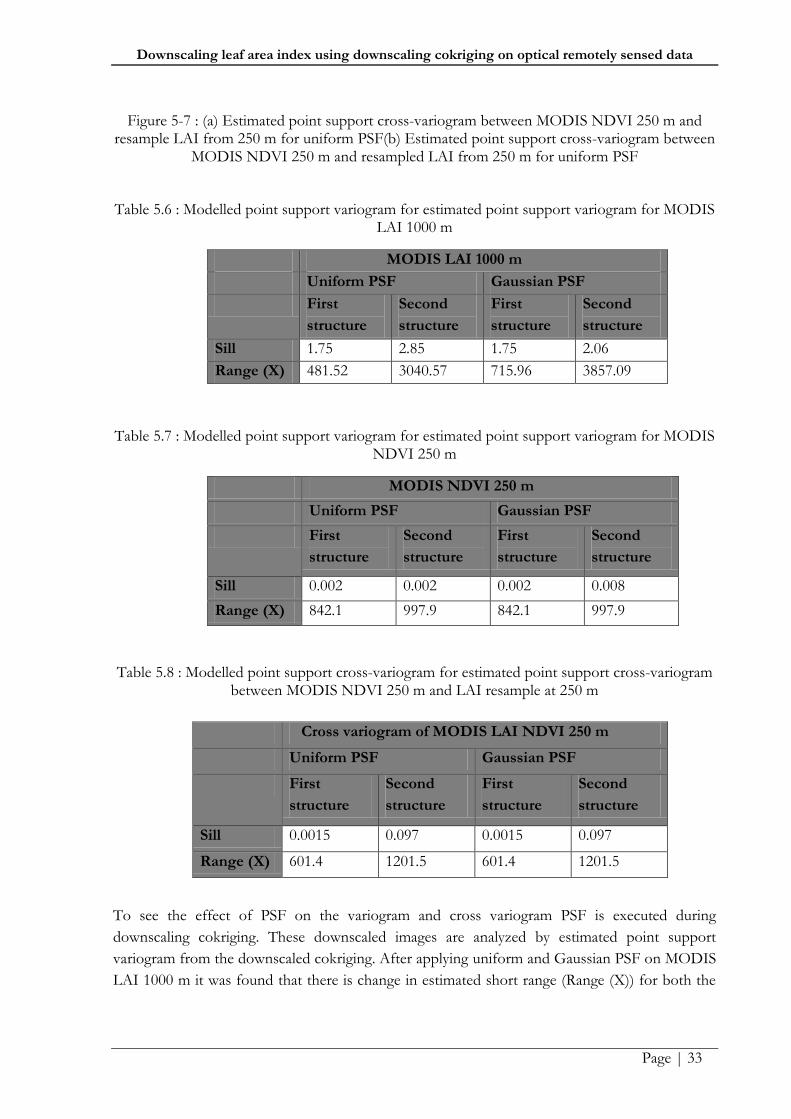
Downscaling leaf area index using downscaling cokriging on optical remotely sensed data
Page | 33
Figure 5-7 : (a) Estimated point support cross-variogram between MODIS NDVI 250 m and resample LAI from 250 m for uniform PSF(b) Estimated point support cross-variogram between
MODIS NDVI 250 m and resampled LAI from 250 m for uniform PSF
Table 5.6 : Modelled point support variogram for estimated point support variogram for MODIS LAI 1000 m
MODIS LAI 1000 m
Uniform PSF Gaussian PSF
First
structure
Second
structure
First
structure
Second
structure
Sill 1.75 2.85 1.75 2.06
Range (X) 481.52 3040.57 715.96 3857.09
Table 5.7 : Modelled point support variogram for estimated point support variogram for MODIS NDVI 250 m
MODIS NDVI 250 m
Uniform PSF Gaussian PSF
First
structure
Second
structure
First
structure
Second
structure
Sill 0.002 0.002 0.002 0.008
Range (X) 842.1 997.9 842.1 997.9
Table 5.8 : Modelled point support cross-variogram for estimated point support cross-variogram between MODIS NDVI 250 m and LAI resample at 250 m
To see the effect of PSF on the variogram and cross variogram PSF is executed during
downscaling cokriging. These downscaled images are analyzed by estimated point support
variogram from the downscaled cokriging. After applying uniform and Gaussian PSF on MODIS
LAI 1000 m it was found that there is change in estimated short range (Range (X)) for both the
Cross variogram of MODIS LAI NDVI 250 m
Uniform PSF Gaussian PSF
First
structure
Second
structure
First
structure
Second
structure
Sill 0.0015 0.097 0.0015 0.097
Range (X) 601.4 1201.5 601.4 1201.5

Downscaling leaf area index using downscaling cokriging on optical remotely sensed data
Page | 34
PSF which is described in table 5-6. It is observed that range for the Gaussian PSF is more than
the uniform PSF and also sill for Gaussian PSF is more than that of uniform PSF.
Using uniform and Gaussian PSF for NDVI does not show any change in sill and range as
shown in table 5-7 but there is difference in the variogram where variance and lag was different
which is shown in figure 5-6 (a) and 5-6 (b) and also minimum variance is very slightly less for
uniform PSF i.e (0.000181) than Gaussian PSF i.e. (0.000154) which is negligible.
There is also no change seen in the sill and range of the estimated cross-variogram after using
uniform and Gaussian PSF. As shown in table 5-8 it has been noticed that the sill and the range
for both are similar for the first structure of uniform and Gaussian PSF and the sill and the range
for second structure are also similar. There is also approximately no change in variogram as
shown in figure 5-8 (a) and (b).
5.4. Impact of PSF on downscaling cokriging
There is impact of PSF on estimating the cokriging weights. The point support models are used
for calculating these weights for both finer (MODIS LAI 1000 m) and coarser resolution images
(MODIS NDVI 250 m). These weights act as a high pass filter and low pass filter. Once these
weights are calculated then they are applied as a window to obtain desired fine resolution image.
These weights are estimated with the use of support on the predicted variable given in equation
4.2.
It can be seen that there is change in the weights after applying the uniform and Gaussian PSF.
The example of weight for 3 x 3 window applied on MODIS LAI 1000 m using uniform PSF is
given in table 5-9 (a) and weight for 4 x 4 window applied on MODIS NDVI 250 m using
uniform PSF is given in table 5-9 (b). Same using Gaussian PSF the example of weights for 3 x 3
window applied on MODIS LAI 1000 m and weights for 4 x 4 window applied on MODIS
NDVI 250 m is given in table 5-10 (a) and 5-10 (b). The sum of the weights of the high pass filter
applied on MODIS LAI 1000 m estimated image are nearly 1.0 and sum of the weights of low
pass filter applied on MODIS NDVI 250 m estimated image are nearly zero which implies the
unbiased condition to set up a unbiased cokriging system.

Downscaling leaf area index using downscaling cokriging on optical remotely sensed data
Page | 35
Table 5.9 :(a) Example of Cokriging weights of 3 x 3 window which act as high pass filter for coarser resolution image (MODIS LAI 1000 m) obtained by using uniform PSF (b) Example of
Cokriging weights of 4 x 4 window which act as low pass filter for finer resolution image (MODIS NDVI 250 m) obtained by using uniform PSF
A11
A12
0.083 0.357 -0.146 0.042 0.407 -0.137
0.198 0.668 -0.033 -0.098 0.924 -0.031
0.030 -0.182 0.027 0.063 -0.186 0.017
A13 A14
0.003 0.380 -0.054 -0.001 0.217 0.123
-0.180 0.916 0.043 -0.162 0.734 0.222
0.030 -0.132 -0.008 0.002 -0.070 -0.065
(a)
a11 a12
-1.039 -0.667 -0.820 -0.751 -1.103 -0.738 -0.821 -0.637
0.835 0.373 -1.760 0.319 0.933 0.451 -1.688 0.332
-0.396 1.352 5.855 2.518 -0.191 1.211 5.837 2.541
0.159 -0.595 -2.845 -2.537 0.411 -0.731 -3.057 -2.747
a13 a14
-1.145 -0.707 -0.767 -0.478 -0.935 -0.610 -0.692 -0.578
1.058 0.410 -1.789 0.281 0.977 0.368 -1.830 0.176
-0.358 1.261 5.947 2.458 -0.516 1.347 5.955 2.433
0.073 -0.854 -3.206 -2.184 -0.206 -0.830 -3.066 -1.991
(b)

Downscaling leaf area index using downscaling cokriging on optical remotely sensed data
Page | 36
Table 5.10 : (a) Example of Cokriging weights of 3 x 3 window which act as high pass filter for coarser resolution image (MODIS LAI 1000 m) obtained by using Gaussian PSF: (b) Example of
Cokriging weights of 4 x 4 window which act as low pass filter for finer resolution image (MODIS NDVI 250 m) obtained by using Gaussian PSF
B11 B12
0.285 0.228 -0.111 0.130 0.317 -0.122
0.013 0.583 0.016 -0.149 0.830 0.049
0.063 -0.047 -0.032 0.087 -0.108 0.034
B13 B14
0.035 0.396 -0.079 -0.003 0.412 0.028
-0.169 0.722 0.144 -0.095 0.349 0.321
0.047 -0.070 -0.027 - 0.012 0.034 -0.035
(a)
b11 b12
-2.476 -0.791 -0.746 -1.092 -1.394 -0.847 -1.063 -0.891
1.500 0.540 -2.551 0.721 1.026 0.831 -2.287 0.723
-0.226 1.186 7.426 3.451 -0.174 1.156 8.099 3.313
0.558 -0.321 -3.472 -3.706 0.927 -0.831 -4.724 -3.863
b13 b14
-1.368 -1.409 -1.124 -0.358 -2.424 -1.347 -0.747 -0.463
1.118 0.114 -2.510 0.409 1.602 0.843 -2.794 0.396
-0.085 1.651 8.342 2.498 -0.020 1.582 7.669 2.659
0.268 -1.539 -4.792 -2.214 -0.121 -0.906 -3.553 -2.374
(b)

Downscaling leaf area index using downscaling cokriging on optical remotely sensed data
Page | 37
These changes in weights may also show the effect of uniform and Gaussian PSF on downscaling
cokriging because these weights are used to set up the ordinary cokriging system. These weights
are also responsible for the prediction minimum variance and unbiased condition.
To study the effect of PSF on downscaling cokriging image descriptive statistics have been
calculated i.e. histogram, box plot, minimum, maximum, 1st quartile, 2nd quartile, mean, median
and standard deviation which is given in Table 5-11. This table explains changes at downscaling
levels at uniform PSF and Gaussian PSF. The impact of PSF can be noticed on downscaled
image in figure 5-8 and 5-9.
Figure 5-8 : Downscaled image of MODIS LAI at 250 m using uniform PSF
Figure 5-9 : Downscaled image of MODIS LAI at 250 m using Gaussian PSF
.
LAI
LAI

Downscaling leaf area index using downscaling cokriging on optical remotely sensed data
Page | 38
(a) (b)
Figure 5-10 : (a) Histogram of LAI showing occurrence of downscaled MODIS LAI at 250 m using uniform PSF (b) Histogram of LAI showing occurrence of downscaled MODIS LAI at 250
m using Gaussian PSF
(a) (b)
Figure 5-11 : (a) Boxplot of LAI showing distribution of downscaled MODIS LAI at 250 m using uniform PSF(b) Boxplot of LAI showing distribution of downscaled MODIS LAI at 250 m using
Gaussian PSF
Histogram in figure 5-10 (a) and 5-10 (b) is showing the distribution of LAI at different
downscaling level and it also shows LAI value from 4.5 to 5 has high occurrence in downscaled
250 m using uniform PSF and in figure 5-10 (b) the downscaled image with Gaussian PSF of 250
m has high occurrence in LAI value 4 to 5. From the histogram it can also be noticed that the
range of LAI value are more in gaussian PSF than that of uniform PSF.

Downscaling leaf area index using downscaling cokriging on optical remotely sensed data
Page | 39
5.4.1. Comparison between downscaled image using uniform PSF and Gaussian PSF
Descriptive statistic has been calculated at different downscaling level which is given below in
Table 5-11:
Table 5.11 : Spatial distribution of downscaled LAI value obtained by using uniform and Gaussian PSF
With uniform PSF With Gaussian PSF
Disaggregation
level
4 x 4 4 x 4
Pixel size (m) 1000 250 1000 250
Minimum 0.6 -0.108 0.6 -0.755
1st Quartile 1.775 1.808 1.775 1.911
Mean 3.405 3.407 3.405 3.408
Median 3.950 3.636 3.950 3.621
3rd Quartile 4.90 4.854 4.90 4.855
Maximum 6.0 7.408 6.0 8.032
SD 1.64 1.73 1.64 1.691
Descriptive statistics shows changes in the minimum, maximum, 1st quartile, 3rd quartile and
standard deviation for downscaled image obtained using uniform and Gaussian PSF which can
be observed in the box plot in figure 5.17 (a) and 5.17 (b). This has also been observed that there
is approximately no change in mean and median and also there is increase in standard deviation
while the resolution is increased using uniform and Gaussian PSF. To show the spatial
dependence in downscaled image using uniform and Gaussian PSF auto-covariance is estimated
for the 10th row in the image for maximum lag 10 which is given in table 5.11. Auto-covariance is
the mesure of spatial dependece between different lags. This autocovariance is calculated by
calculating covariance at sucessive lags. This auto-covariance shows the spatial association and
spatial correlation between the variable. This auto-covariance depicts spatial variation and spatial
dependence in the image. It is observed that as the lag is increasing correlation and auto-
covariance is decreasing. It is found that using uniform PSF there are some negative value at lag 9
and 10.

Downscaling leaf area index using downscaling cokriging on optical remotely sensed data
Page | 40
Table 5.12: Auto-covariance between downscaled image using uniform and Gaussian PSF
Using Uniform PSF
Using Gaussian PSF
Lag Cov r(correlation) Cov r(correlation)
0 2.95 1 2.89 1
1 2.86 0.96 2.74 0.94
2 2.56 0.86 2.52 0.87
3 2.11 0.71 2.24 0.77
4 1.60 0.54 1.86 0.64
5 1.13 0.38 1.56 0.54
6 0.70 0.23 1.22 0.42
7 0.34 0.11 0.87 0.30
8 0.07 0.02 0.57 0.19
9 -0.08 -0.02 0.36 0.12
10 -0.15 -0.05 0.20 0.07
5.5. Summary of the Results
The results obtained from this research are summarized on the effect of resampling on
variogram, effect of PSF on variogram and downscaling cokriging.
It was found that trivial method is better to resample coarse resolution (LAI) to calculate sample
cross-variogram. This technique shows more variance than the other resampling techniques. The
uniform PSF shows the more spatial dependence than the Gaussian PSF.
Due to spatial variability or change in variance in point support variogram and cross-variogram
the cokriging weights were found different for both the PSF and further which show changes in
the downscaled cokriging image. These changes in the spatial distribution are explained by
calculating minimum, maximum, mean, standard deviation in the LAI values. To show the spatial
dependence auto-covariance was estimated which shows that uniform PSF has more spatial
dependence than the Gaussian PSF.

Downscaling leaf area index using downscaling cokriging on optical remotely sensed data
Page | 41
6. DISCUSSION
The research has demonstrated the effect of resampling and PSF on downscaling cokriging
technique by showing the selection of covariable by estimating the coefficient of correlation, the
effect of resampling on variogram and cross-variogram, effect of PSF on variogram and cross
variogram and effect of PSF on downscaling cokriging.
6.1. Correlation of LAI with NDVI, NIR and Red bands from optical image
Cokriging is multivariate area-to-point prediction approach. Downscaling using cokriging require
a covariable to downscale LAI (primary variable). This covariable must have a relationship with
primary variable. In this study for selecting the covariable correlation analysis has been done.
Correlation analysis has been executed between primary variable LAI and covariable NDVI, Near
Infrared reflectance band and red reflectance bands which are shown in table 5.1. From
correlation analysis the relationship between LAI and NDVI is found positive (r = 0.58) and
significant (p < 0.01). (Kale et al., 2005) found in his study that for relationship between LAI and
NDVI the minimum correlation is r = 4 and maximum correlation is r = 7.4. In the month of
October Barkot forest is full of vegetation due to which NDVI is high. Due to this high NDVI
the correlation with LAI is high. Correlation of NIR (r = 0.47) is found less than NDVI with
LAI at significant (p < 0.01) which is less than correlation with NDVI. A small relationship was
found between LAI and red reflectance (r = 0.001) at significant (p < = 0.001). (Kaufman et al.,
2002) stated that low correlation for the red reflectance is due to mixed vegetation and bright soil
and red reflectance show high absorption in vegetation due to chlorophyll absorption. So
relationship between LAI and NDVI is found more in compare to NIR and red reflectance.
6.2. Impact of resampling on the variogram and cross variogram
In this study coarser resolution image (MODIS LAI 1000 m) and finer resolution image (MODIS
NDVI 250 m) is combinined to predict finer resolution image of MODIS LAI at 250 m. To
estimate cross-variogram for estimating cross-covariance coarser and finer resolution were
brought to a common resolution by resampling technique. NN, CC, BI and trivial resampling
methods were executed to resample pixel of coarser resolution to finer resolution. The sample
cross-variogram were calculated to see the effect of resampling at the common cut-off of 6000
m, bin of 15 and then modelled by using exponential model at a common range of 3817.4 m.
This common range was choosen visually for linear model of coregionalization.
It was observed from the table 5-2, 5-3, 5-4, 5-5 that the sill and nugget are varying for all
resampling methods in sample cross-variogram. It was observed that model was best fit to NN
resampling and trivial resampling. The sill from trivial and NN resampling was found to be
higher than that of CC and BI resampling which depicts that the variance is high at the range of
3817.4 in NN and trivial resampling. This high variance may be due to the resampled LAI value.
In trivial method the values remain same, while in the nearest neighbour resampling the values

Downscaling leaf area index using downscaling cokriging on optical remotely sensed data
Page | 42
was approximately the same because it interpolates by taking the average of the nearest pixel
value whereas the variance in CC and BI resampling is low due to which there is less spatial
structure. So, for this research the trivial method was used in calculating sample variogram.
6.3. Impact of PSF on variogram and cross-variogram
The impact of the PSF on the variogram was studied by estimating the variogram to estimate
point support variogram. These point support variogram were estimated for both the image using
uniform and Gaussian PSF. In this study point support variogram were modelled by nested
exponential structure of variogram at a common cut-off of 6000 m and bin of 15. It has been
observed that for MODIS LAI 1000 m modelled point support variogram has a sill for first
structure of 1.75 for uniform and Gaussian PSF at different range of 481.52m and 715.96 m and
sill for second structure is 2.85 for uniform PSF and 2.068 for Gaussian PSF at range of 3040.57
m and 3857.09 m which is shown in table 5-6. It could be due to weight contributing in the pixel
for Gaussian function which is more in the centre of pixel than the border of the pixel and for
uniform PSF weights are uniform in the centre and at the border of the pixel. This change in sill
may be due to the distance from the centre of the pixel is high. The distance from the centre of
pixel is more for uniform PSF rather than Gaussian PSF which is shown in figure 5-5 (a) and (b).
It can be noticed that for the same distance there is change in the variance which is due to change
of pixel value which is high using uniform PSF.
Impact of PSF was not seen in the modelled point support variogram from MODIS NDVI 250
m as shown in table 5.7. The sill and the range of the first structure of uniform PSF and Gaussian
PSF are same and for second structure sill and range are same, but there is a change in point
supports variogram which can be observed in figure 5-6 (a) and (b). This change may be due to
effect of and which affects the imaging response of the image where the response within
the pixel is uniform and very less response from the outside of the pixel which may be due to
atmospheric effect and geometry of the view (Huang et al., 2002)
Also no change has been noticed in the sill and the range of modelled estimated point support
cross-variogram after using uniform and Gaussian PSF. As shown in table 5.8 it has been noticed
that sill and range for the first structure of uniform PSF are similar and sill and the range for the
second structure of uniform PSF and Gaussian PSF are similar and there is a no change in the
point support cross-variogram also because there is no effect of PSF in point support cross-
covariances (Pardo-Iguzquiza et al., 2006)
6.4. Impact of PSF on downscaling cokriging
To study the effect of PSF on downscaling cokriging the change in the weights are analyzed. As
PSF plays an important role in setting up the unbiased cokriging weights for the ordinary
cokriging system. Cokriging predictor is the function of cokriging weights and random variable.
These random variables are related to variance which implies that variance is related to the
cokriging weights. This indicates that if variance is high then weights will be high (Pardo-

Downscaling leaf area index using downscaling cokriging on optical remotely sensed data
Page | 43
Iguzquiza et al., 2011). The variance is high using uniform PSF rather than Gaussian PSF. From
the table 5-9 and 5-10 it is observed that for uniform PSF and Gaussian PSF weights are different
which is due to variance and for uniform PSF weights are more than that of Gaussian PSF. It can
be also observed from the table 5-9 (a) and 5-10 (a) that the centre value of weights obtained by
using uniform PSF is more than that of Gaussian PSF. Gaussian PSF is related to standard
deviation in the pixel while uniform PSF does not involve the standard deviation. This indicates
that the mean of the centre pixel of Gaussian support is more than that uniform PSF which
affect the centre of the weights in inversely, as this mean is subtracted from the random function
in the cokriging predictor so large is the mean small will be the weights.
It is also observed from the figure 5-8 and 5-9 that due to weights applied for downscaling, a
blurring effect is visualized in downscaled image using gaussian PSF. It can be observed that the
variance is less using Gaussian PSF than using uniform PSF due to which it is more difficult to
visualize the object. This is due to the less spatial variability and smoothness in the image.
To study the effect of PSF on the downscaled images histogram has been estimated. Histogram
in figure 5.10 (a) and 5.10 (b) it is observed that distribution of LAI value is approximately same
for both the downscaled image using uniform and Gaussian PSF. In descriptive statistics from
table 5-11 it is observed that there changes in minimum, maximum, 1st quartile, 3rd quartile and
standard deviation in downscaled image using uniform and Gaussian PSF. This variation show
there is a spatial variability in the downscaled LAI value though there is no clear pattern found. It
is observed that standard deviation is more in uniform PSF which shows that there are more
changes in LAI value than the Gaussian PSF though it depends on the distance from the centre
of the pixel. It is also observed from table 5-12 that with the increase in the distance between the
point pairs covariance decreases and also correlation also decreases. It is also observed that using
Gaussian PSF covariance and correlation between the variables are higher and positive which
shows the data at a closer distance are more similar to each other and using uniform PSF it is less
spatially dependent because of gradual change in pixel in downscaled image using gaussian PSF.

Downscaling leaf area index using downscaling cokriging on optical remotely sensed data
Page | 44
7. CONCLUSION AND RECOMMENDATIONS
7.1. Conclusions
The main objective of this research is to study the effect of resampling and PSF on downscaling cokriging technique for LAI estimation. To achieve this objective four research questions were carried out in this study. An attempt is made to answer these research questions and conclusion for each question is given as: 1. What is the suitable covariable and its correlation with LAI? NDVI and LAI relationship has been used to estimate LAI which has been seen in many researches as mentioned in literature review point 2.5. From this study it was found that out of variable considered i.e. infro-red, red and NDVI, NDVI is a suitable covariable to downscale LAI, though it shows a good relationship with LAI. Red reflectance and NIR reflectance does not show good relationship with LAI. It can be seen from the table 4.1 that correlation between LAI and NDVI is r = 5.8. 2. What is the effect of resampling on variogram and cross-variogram? It was shown from the results 5.2 that there is change observed by applying the different resampling techniques. The NN and trivial method shows a high variance which means that there is more spatial structure. The trivial method is used for calculating the sample cross-variogram because of more spatial structure and the values did not changes after resampling of LAI from 1000 m to 250 m. 3. What is the effect of PSF on variogram and cross-variogram? It was found from this study that for coarser resolution there is a change noticed in the estimated point support variogram using uniform PSF and Gaussian PSF. This change is due to the mean and standard deviation within the pixel. The change in the PSF is due to the response by distance from the centre of the pixel. The effects are also due to effect within the pixel and outside of the pixel while no change was observed in the cross-variogram. 4. What is the effect of PSF on resultant downscaled image? To study the effect of PSF on downscaled image change in weight were observed at different PSF i.e. uniform and Gaussian PSF. Cokriging weights are related to covariance and cross-covariance. It was observed that variance is high in uniform PSF so the weights were high for the uniform PSF. These variances can be observed from the analysis of estimated point support variogram by observing sill, nugget and range. It is also found that quality of the image also depends on the PSF. Gaussian PSF shows the better quality than by using uniform PSF Finally it is concluded that for NDVI is a suitable covariable to downscale LAI. Resampling by trivial method is optimal because it does not affect the LAI value after resampling. Point support function involved in the prediction has an effect on the estimating point support covariance and cross-covariance. The effect of PSF can be studied on estimating point support variogram and cross-variogram. The effect of PSF on the downscaled cokriging image can be observed by change in the cokriging weights. This change in the weights is due to variation in the covariance

Downscaling leaf area index using downscaling cokriging on optical remotely sensed data
Page | 45
and cross-covariance, centre mean of the pixel and the distance between point pairs. It is also observed that downscaled image using Gaussian PSF is more spatially dependent than using uniform PSF due to more variance in constant PSF.
7.2. Recommendation
The downscaling cokriging downscaling is performed on a target variable by using covariable.
More than one covariable can be used to perform downscaling. Ground measurement and
thematic maps may be considered as covariable. Different study area can be used. User define
PSF may be used to study the PSF effect. This study may be carried out with different window
size and study its effect. Different standard deviation may be experiment and field must be used
for the validation.

Page | 46
REFERENCES
Asner, G.P., Braswell, B.H., Schimel, D.S., Wessman, C.A., 1998. Ecological research needs
from multiangle remote sensing data. Remote Sensing of Environment 63(2), 155-165.
Asner, G.P., Scurlock, J.M.O., A. Hicke, J., 2003. Global synthesis of leaf area index
observations: implications for ecological and remote sensing studies. Global Ecology and
Biogeography 12(3), 191-205.
Atkinson, P.M., 2012. Downscaling in remote sensing. International Journal of Applied Earth
Observation and Geoinformation.
Atkinson, P.M., Curran, P.J., 1995. Defining an optimal size of support for remote sensing
investigations. IEEE Transactions on Geoscience and Remote Sensing, 33(3), 768-776.
Atkinson, P.M., Cutler, M.E.J., Lewis, H., 1997. Mapping sub-pixel proportional land cover
with AVHRR imagery. International Journal of Remote Sensing 18(4), 917-935.
Baboo, S.S., Devi, M.R., 2010. An analysis of different resampling methods in Coimbatore,
district. Global Journal of Computer Science and Technology 10(15), 61-66.
Bannari, A., Morin, D., Bonn, F., Huete, A.R., 1995. A review of vegetation indices. Remote
Sensing Reviews 13(1-2), 95-120.
Baret, F., Guyot, G., 1991. Potentials and limits of vegetation indices for LAI and APAR
assessment. Remote Sensing of Environment 35(2–3), 161-173.
Chen, J.M., Leblanc, S.G., 1997. A four-scale bidirectional reflectance model based on
canopy architecture. IEEE Transactions on Geoscience and Remote Sensing, 35(5), 1316-
1337.
Curran, P., 1980. Relative reflectance data from preprocessed multispectral photography.
International Journal of Remote Sensing 1(1), 77-83.
DAAC, U.L., 2013. https://lpdaac.usgs.gov/products/modis_products_table/mod13q1.
(accessed 7 January ).
eXtension, 2008. Remote sensing resampling methods.
http://www.extension.org/pages/9628/remote-sensing-resampling-methods (accessed
February 1, 2013).
Fassnacht, K.S., Gower, S.T., MacKenzie, M.D., Nordheim, E.V., Lillesand, T.M., 1997.
Estimating the leaf area index of North Central Wisconsin forests using the landsat thematic
mapper. Remote Sensing of Environment 61(2), 229-245.
Fassnacht, K.S., Gower, S.T., Norman, J.M., McMurtric, R.E., 1994. A comparison of optical
and direct methods for estimating foliage surface area index in forests. Agricultural and
Forest Meteorology 71(12), 183-207.

Page | 47
Feng, C., Ma, J., Chen, J., 2004. The PSF correction method for satellite image restoration,
IEEE First Symposium on Multi-Agent Security and Survivability, 2004 pp. 31-34.
Goldsmith, N., 2009. Resampling raster images.
http://www.jiscdigitalmedia.ac.uk/stillimages/advice/resampling-raster-images/ (accessed
February 1, 2013).
Goodale, C.L., Apps, M.J., Birdsey, R.A., Field, C.B., Heath, L.S., Houghton, R.A., Jenkins,
J.C., Kohlmaier, G.H., Kurz, W., Liu, S., Nabuurs, G., Nilsson, S., Shvidenko, A.Z., 2002.
Forest carbon sinks in the northern hemisphere. Ecological Applications 12(3), 891-899.
Gower, S.T., Kucharik, C.J., Norman, J.M., 1999. Direct and Indirect Estimation of Leaf Area
Index, fAPAR, and Net Primary Production of Terrestrial Ecosystems. Remote Sensing of
Environment 70(1), 29-51.
Hu, J., Tan, B., Shabanov, N., Crean, K.A., Martonchik, J.V., Diner, D.J., Knyazikhin, Y.,
Myneni, R.B., 2003. Performance of the MISR LAI and FPAR algorithm: a case study in
Africa. Remote Sensing of Environment 88(3), 324-340.
Huang, C., Townshend, J.R.G., Liang, S., Kalluri, S.N.V., DeFries, R.S., 2002. Impact of
sensor's point spread function on land cover characterization: assessment and deconvolution.
Remote Sensing of Environment 80(2), 203-212.
Hwang, T., Song, C., Bolstad, P.V., Band, L.E., 2011. Downscaling real-time vegetation
dynamics by fusing multi-temporal MODIS and Landsat NDVI in topographically complex
terrain. Remote Sensing of Environment 115(10), 2499-2512.
Jeganathan, C., Hamm, N., Mukherjee, S., Atkinson, P.M., Raju, P.L.N., Dadhwal, V.K.,
2011. Evaluating a thermal data sharpening technique over a mixed agricultural landscape in
India. International Journal of Applied Earth Observation and Geoinformation 13, 178-191.
Jonckheere, I., Fleck, S., Nackaerts, K., Muys, B., Coppin, P., Weiss, M., Baret, F., 2004.
Review of methods for in situ leaf area index determination: Part I. Theories, sensors and
hemispherical photography. Agricultural and Forest Meteorology 121(1–2), 19-35.
Kale, M., Singh, S., Roy, P.S., 2005. Estimation of Leaf Area Index in dry deciduous forests
from IRS WiFS in central India. International Journal of Remote Sensing 26(21), 4855-4867.
Kaufman, Y.J., Gobron, N., Pinty, B., Widlowski, J., Verstraete, M.M., 2002. Relationship
between surface reflectance in the visible and mid-IR used in MODIS aerosol algorithm -
theory. Geophysical Research Letters 29(23), 2116.
Kustas, W.P., Norman, J.M., Anderson, M.C., French, A.N., 2003. Estimating sub-pixel
surface temperatures and energy fluxes from the vegetation indexradiometric temperature
relationship. Remote Sensing of Environment 85, 429-440.
Maki, M., Nishida, K., Saigusa, N., Akiyama, T., 2005. Evaluation of the relationship
between NDVI and LAI in cool-temperate deciduous forest, The Proceeding of Asian
Conference of Remote Sensing.

Page | 48
Miller, J.R., White, H.P., Chen, J.M., Peddle, D.R., McDermid, G., Fournier, R.A., Shepherd,
P., Rubinstein, I., Freemantle, J., Soffer, R., LeDrew, E., 1997. Seasonal change in understory
reflectance of boreal forests and influence on canopy vegetation indices. Journal of
Geophysical Research: Atmospheres 102(D24), 29475-29482.
Mustafa, Y.T., Van Laake, P.E., Stein, A., 2011. Bayesian network modeling for improving
forest growth estimates. IEEE Transactions on Geoscience and Remote Sensing, 49(2), 639-
649.
Myneni, R., Knyazikhin, Y., Glassy, J., Votava, P., Shabanov, N., 2003. User's Guide FPAR,
LAI (ESDT: MOD15A2) 8-day Composite NASA MODIS Land Algorithm.
http://cybele.bu.edu/modismisr/products/modis/userguide.pdf (accessed February 27, 2013).
Myneni, R.B., Hoffman, S., Knyazikhin, Y., Privette, J.L., Glassy, J., Tian, Y., Wang, Y.,
Song, X., Zhang, Y., Smith, G.R., Lotsch, A., Friedl, M., Morisette, J.T., Votava, P., Nemani,
R.R., Running, S.W., 2002. Global products of vegetation leaf area and fraction absorbed
PAR from year one of MODIS data. Remote Sensing of Environment 83(1–2), 214-231.
Ollinger, S.V., 2003. Forest ecosystems. http://www.els.net/WileyCDA/ElsArticle/refId-
a0003190.html (accessed 5 February, 2013).
Pandya, M.R., Singh, R.P., Chaudhari, K.N., Bairagi, G.D., Sharma, R., Dadhwal, V.K.,
Parihar, J.S., 2006a. Leaf area index retrieval using IRS LISS-III sensor data and validation of
the MODIS LAI product over central India. IEEE Transactions on Geoscience and Remote
Sensing 44(7), 1858-1865.
Pandya, M.R., Singh, R.P., Chaudhari, K.N., Bairagi, G.D., Sharma, R., Dadhwal, V.K.,
Parihar, J.S., 2006b. Leaf area index retrieval using IRS LISS-III sensor data and validation of
the MODIS LAI product over central India. IEEE Transactions on Geoscience and Remote
Sensing, 44(7), 1858-1865.
Pardo-Iguzquiza, E., Atkinson, P.M., 2007. Modelling the semivariograms and cross-
semivariograms required in downscaling cokriging by numerical convolution-deconvolution.
Computers & Geosciences 33(10), 1273-1284.
Pardo-Iguzquiza, E., Atkinson, P.M., Chica-Olmo, M., 2010. DSCOKRI: A library of
computer programs for downscaling cokriging in support of remote sensing applications.
Computers & Geosciences 36(7), 881-894.
Pardo-Iguzquiza, E., Chica-Olmo, M., Atkinson, P.M., 2006. Downscaling cokriging for
image sharpening. Remote Sensing of Environment 102(12), 86-98.
Pardo-Iguzquiza, E., Rodríguez-Galiano, V.F., Chica-Olmo, M., Atkinson, P.M., 2011. Image
fusion by spatially adaptive filtering using downscaling cokriging. ISPRS Journal of
Photogrammetry and Remote Sensing 66(3), 337-346.
Peng, G., Ruiliang, P., Biging, G.S., Larrieu, M.R., 2003. Estimation of forest leaf area index
using vegetation indices derived from Hyperion hyperspectral data. Geoscience and Remote
Sensing, IEEE Transactions on 41(6), 1355-1362.

Page | 49
Pouteau, R., Rambal, S., Ratte, J.-P., Gogé, F., Joffre, R., Winkel, T., 2011. Downscaling
MODIS-derived maps using GIS and boosted regression trees: The case of frost occurrence
over the arid Andean highlands of Bolivia. Remote Sensing of Environment 115(1), 117-129.
Propastin, P., Erasmi, S., 2010. A physically based approach to model LAI from MODIS
250 m data in a tropical region. International Journal of Applied Earth Observation and
Geoinformation 12(1), 47-59.
Qi, J., Chehbouni, A., Huete, A.R., Kerr, Y.H., Sorooshian, S., 1994. A modified soil adjusted
vegetation index. Remote Sensing of Environment 48(2), 119-126.
Rouse J.W., H.R.H., Schell J.A., Deering D.W., Harlan J.C., 1974. Monitoring the vernal
advancement of retrogradation of natural vegetation. NASA/GSFC, MD.
Running, S.W., Baldocchi, D.D., Turner, D.P., Gower, S.T., Bakwin, P.S., Hibbard, K.A.,
1999. A Global Terrestrial Monitoring Network Integrating Tower Fluxes, Flask Sampling,
Ecosystem Modeling and EOS Satellite Data. Remote Sensing of Environment 70(1), 108-
127.
Singh, S.P., 2010. Impact of forest degradation on carbon density in soil and vegetation of
shorea robusta, Sal, forests in the part of siwalik hills of Dehradun, India, using geospatial
techniques, Applied Earth Obsevation Department. ITC- Faculty of Geo-Information Science
and Earth Observation, The Netherlands, pp. 1-85.
Song, C., 2013. Optical remote sensing of forest leaf area index and biomass. Progress in
Physical Geography 37(1), 98-113.
Spanner, M.A., Pierce, L.L., Peterson, D.L., Running, S.W., 1990. Remote sensing of
temperate coniferous forest leaf area index The influence of canopy closure, understory
vegetation and background reflectance. International Journal of Remote Sensing 11(1), 95-
111.
Spanner, M.A., Pierce, L.L., Peterson, D.L., Running, S.W., 1990(b). Remote sensing of
temperate coniferous forest leaf area index: The influence of canopy closure, understory
vegetation and background reflectance. International Journal of Remote Sensing 11, 95-111.
Spanner, M.A., Pierce, L.L., Running, S.W., Peterson, D.L., 1990(a). The seasonality of
AVHRR data of temperate coniferous forests: Relationship with leaf area index. Remote
Sensing of Environment 33(2), 97-112.
Stathopoulou, M., Cartalis, C., 2009. Downscaling AVHRR land surface temperatures for
improved surface urban heat island intensity estimation. Remote Sensing of Environment
113(12), 2592-2605.
Studley, H., Weber, K.T., 2010. Comparison of image resampling techniques for satellite
imagery, Assessing post-fire recovery of sagebrush steppe rangelands in southeastern Idaho.
GIS Training and Research Center, Idaho, p. 185.

Page | 50
Tian, Y., Woodcock, C.E., Wang, Y., Privette, J.L., Shabanov, N.V., Zhou, L., Zhang, Y.,
Buermann, W., Dong, J., Veikkanen, B., Häme, T., Andersson, K., Ozdogan, M.,
Knyazikhin, Y., Myneni, R.B., 2002. Multiscale analysis and validation of the MODIS LAI
product: I. Uncertainty assessment. Remote Sensing of Environment 83(3), 414-430.
Wade, T., Sommer , S., 2006. A to Z GIS. ESRI Press, Redlands.
Wang, Q., Adiku, S., Tenhunen, J., Granier, A., 2005. On the relationship of NDVI with leaf
area index in a deciduous forest site. Remote Sensing of Environment 94(2), 244-255.
Wilhelm, W.W., Ruwe, K., Schlemmer, M.R., 2000. Comparison of three leaf area index
meters in a corn canopy. Crop Sciences. 40(4), 1179-1183.
Wolf, P.R., Dewitt, B.A., 2004. Elements of photogrammetry with application in GIS, 3rd ed.
McGraw-Hill, Singapore.
Woodcock, C.E., Strahler, A.H., 1987. The factor of scale in remote sensing. Remote Sensing
of Environment 21(3), 311-332.
Zhan, W., Chen, Y., Zhou, J., Li, J., Liu, W., 2011. Sharpening Thermal Imageries: A
Generalized Theoretical Framework From an Assimilation Perspective. IEEE Transactions on
Geoscience and Remote Sensing, 49(2), 773-789.
Zurita-Milla, R., Kaiser, G., Clevers, J.G.P.W., Schneider, W., Schaepman, M.E., 2009.
Downscaling time series of MERIS full resolution data to monitor vegetation seasonal
dynamics. Remote Sensing of Environment 113(9), 1874-1885.

Page | 51

Page | 52
APPENDIX
Appendix 1: R-code to estimate variogram of LAI and NDVI and cross-variogram between
LAI and NDVI
a) Reload package in R software
> require(gstat)
> require(raster)
> require(rgdal)
b) Display Image
> LAI_image <- raster("LAI.img")
> NDVI_image <- raster("NDVI.img")
c) Estimating variogram from LAI image
> M_LAI <- "LAI.img"
> dataset_LAI <- GDAL.open(M_LAI)
> dataset_LAI
> displayDataset(dataset_LAI, band=1, reset.par=FALSE)
> datatable_LAI <- getRasterTable(dataset_LAI, band = NULL, offset = c(0, 0),region.dim =
dim(dataset_LAI))
> datatable_LAI_new <- datatable_LAI[!is.na(datatable_LAI[,3]),]
> datatable_LAI_new
> coordinates(datatable_LAI_new) <- ~x+y
> M_LAI.ev <- variogram(band1~1, data=datatable_LAI_new, cutoff=6000)
d) Estimating variogram from NDVI image
> M_NDVI <- "NDVI.img"
> dataset_NDVI <- GDAL.open(M_NDVI)
> dataset_NDVI
> displayDataset(dataset_NDVI, band=1, reset.par=FALSE)
> datatable_NDVI <- getRasterTable(dataset_NDVI, band = NULL, offset = c(0, 0),region.dim
= dim(dataset_NDVI))
> datatable_NDVI_new <- datatable_NDVI[!is.na(datatable_NDVI[,3]),]
> datatable_NDVI_new
> coordinates(datatable_NDVI_new) <- ~x+y
> M_NDVI.ev <- variogram(band1~1, data=datatable_NDVI_new, cutoff=6000)

Page | 53
e) Estimating Cross-variogram
> g <- gstat(NULL, "M_LAI_250", band1~1, datatable_LAI_new_resample)
> g <- gstat(g, "M_NDVI_250", band1~1, datatable_NDVI_new)
> g
> cross.variogram <- variogram(g, cutoff=6000)