Embed Size (px)
Citation preview
University of Warwick institutional repository: http://go.warwick.ac.uk/wrap
A Thesis Submitted for the Degree of PhD at the University of Warwick
http://go.warwick.ac.uk/wrap/38110
This thesis is made available online and is protected by original copyright.
Please scroll down to view the document itself.
Please refer to the repository record for this item for information to help you tocite it. Our policy information is available from the repository home page.
AUTHOR: Neha Gupta
DEGREE: . . . . . . . . . . . . . . . . . . . . . . . . . . . . . . . . . . . . . . . . . . . . . . . . . . . . . . .
TITLE:HOMOTOPY QUANTUM FIELD THEORY AND
QUANTUM GROUPS
DATE OF DEPOSIT: . . . . . . . . . . . . . . . . . . . . . . . . . . . . . . . . . . . . . . . . . . . . . . . . . . . . . . .
I agree that this thesis shall be available in accordance with the regulations governing the University of
Warwicktheses.
I agree that the summary of this thesis may be submitted for publication.
I agree that the thesis may be photocopied (single copies for study purposes only).
Theses with no restriction on photocopying will also be made available to the British Library for microfilming. The
British Library may supply copies to individuals or libraries. subject to a statement from them that the copy is
supplied for non-publishing purposes. All copies supplied by the British Library will carry the following statement:
“Attention is drawn to the fact that the copyright of this thesis rests with its author. This copy of
the thesis has been supplied on the condition that anyone who consults it is understood to recognise
that its copyright rests with its author and that no quotation from the thesis and no information
derived from it may be published without the author’s written consent.”
AUTHOR’S SIGNATURE: . . . . . . . . . . . . . . . . . . . . . . . . . . . . . . . . . . . . . . . . .
USER DECLARATION
(i) I undertake not to quote or make use of any information from this thesis without making acknowl-
edgement to the author.
(ii) I further undertake to allow no-one else to use this thesis while it is in my care.
DATE SIGNATURE ADDRESS
. . . . . . . . . . . . . . . . . . . . . . . . . . . . . . . . . . . . . . . . . . . . . . . . . . . . . . . . . . . . . . . . . . . . . . . . . . . . . . . . .
. . . . . . . . . . . . . . . . . . . . . . . . . . . . . . . . . . . . . . . . . . . . . . . . . . . . . . . . . . . . . . . . . . . . . . . . . . . . . . . . .
. . . . . . . . . . . . . . . . . . . . . . . . . . . . . . . . . . . . . . . . . . . . . . . . . . . . . . . . . . . . . . . . . . . . . . . . . . . . . . . . .
. . . . . . . . . . . . . . . . . . . . . . . . . . . . . . . . . . . . . . . . . . . . . . . . . . . . . . . . . . . . . . . . . . . . . . . . . . . . . . . . .
. . . . . . . . . . . . . . . . . . . . . . . . . . . . . . . . . . . . . . . . . . . . . . . . . . . . . . . . . . . . . . . . . . . . . . . . . . . . . . . . .
HOMOTOPY QUANTUM FIELD THEORY ANDQUANTUM GROUPS
by
Neha Gupta
Thesis
Submitted to the University of Warwick
for the degree of
Doctor of Philosophy
Supervisors: Dr Dmitriy Rumynin
Department of Mathematics
February 2011
HOMOTOPY QUANTUM FIELD THEORY ANDQUANTUM GROUPS
by
Neha Gupta
Thesis
Submitted to the University of Warwick
for the degree of
Doctor of Philosophy
Supervisors: Dr Dmitriy Rumynin
Department of Mathematics
February 2011
Contents
1 Introduction 5
2 Basic Results 17
2.1 Category Theory . . . . . . . . . . . . . . . . . . . . . . . . . . . . . . . . 17
2.2 Crossed modules . . . . . . . . . . . . . . . . . . . . . . . . . . . . . . . . 27
2.3 Cohomology of groups . . . . . . . . . . . . . . . . . . . . . . . . . . . . . 28
2.4 Duality and Pairings . . . . . . . . . . . . . . . . . . . . . . . . . . . . . . 30
2.5 Schemes . . . . . . . . . . . . . . . . . . . . . . . . . . . . . . . . . . . . . 31
2.5.1 Algebraic Groups . . . . . . . . . . . . . . . . . . . . . . . . . . . . 35
2.6 Sheaves . . . . . . . . . . . . . . . . . . . . . . . . . . . . . . . . . . . . . 37
2.6.1 Tensor product . . . . . . . . . . . . . . . . . . . . . . . . . . . . . 38
2.6.2 G-equivariant sheaves . . . . . . . . . . . . . . . . . . . . . . . . . 39
2.6.3 Cosheaves . . . . . . . . . . . . . . . . . . . . . . . . . . . . . . . . 40
2.7 Disjoint Union . . . . . . . . . . . . . . . . . . . . . . . . . . . . . . . . . 45
2.8 Orientation . . . . . . . . . . . . . . . . . . . . . . . . . . . . . . . . . . . 47
2.9 HQFT . . . . . . . . . . . . . . . . . . . . . . . . . . . . . . . . . . . . . . 50
2.9.1 Preliminaries on HQFTs. . . . . . . . . . . . . . . . . . . . . . . . 51
2.9.2 Definition of an HQFT . . . . . . . . . . . . . . . . . . . . . . . . . 52
3 Crossed Systems 57
3.1 G-coalgebras . . . . . . . . . . . . . . . . . . . . . . . . . . . . . . . . . . 57
3.2 Frobenius graded systems . . . . . . . . . . . . . . . . . . . . . . . . . . . 60
3.2.1 Frobenius systems . . . . . . . . . . . . . . . . . . . . . . . . . . . 60
1
CONTENTS
3.2.2 Frobenius graded systems . . . . . . . . . . . . . . . . . . . . . . . 65
3.3 Cobordism category . . . . . . . . . . . . . . . . . . . . . . . . . . . . . . 70
3.4 Crossed Systems . . . . . . . . . . . . . . . . . . . . . . . . . . . . . . . . 83
3.4.1 Reduced category : X − Cobn . . . . . . . . . . . . . . . . . . . . . 84
3.4.2 Turaev crossed system . . . . . . . . . . . . . . . . . . . . . . . . . 88
3.4.3 K(G,n+1) case . . . . . . . . . . . . . . . . . . . . . . . . . . . . . 90
3.4.4 K(G,1) case . . . . . . . . . . . . . . . . . . . . . . . . . . . . . . . 91
3.4.5 Cylinders and X -Cylinders . . . . . . . . . . . . . . . . . . . . . . 97
3.5 HQFTs . . . . . . . . . . . . . . . . . . . . . . . . . . . . . . . . . . . . . 103
3.5.1 Computing τ . . . . . . . . . . . . . . . . . . . . . . . . . . . . . . 104
3.6 Examples . . . . . . . . . . . . . . . . . . . . . . . . . . . . . . . . . . . . 125
3.6.1 Crossed module . . . . . . . . . . . . . . . . . . . . . . . . . . . . . 125
3.6.2 Twisted category . . . . . . . . . . . . . . . . . . . . . . . . . . . . 129
3.6.3 Crossed module in a twisted category . . . . . . . . . . . . . . . . 136
4 Coloured Quantum groups 146
4.1 G-coalgebras . . . . . . . . . . . . . . . . . . . . . . . . . . . . . . . . . . . 146
4.2 Hopf G-coalgebras . . . . . . . . . . . . . . . . . . . . . . . . . . . . . . . 152
4.2.1 Hopf group-coalgebras . . . . . . . . . . . . . . . . . . . . . . . . . 153
4.2.2 Hopf G-coalgebras . . . . . . . . . . . . . . . . . . . . . . . . . . . 154
4.2.3 Crossings . . . . . . . . . . . . . . . . . . . . . . . . . . . . . . . . 160
4.2.4 Quasitriangularity . . . . . . . . . . . . . . . . . . . . . . . . . . . 162
4.3 Affine case . . . . . . . . . . . . . . . . . . . . . . . . . . . . . . . . . . . . 164
4.3.1 Structure of a Hopf G-coalgebra . . . . . . . . . . . . . . . . . . . . 164
4.3.2 Crossings . . . . . . . . . . . . . . . . . . . . . . . . . . . . . . . . 165
4.3.3 Quasitriangularity . . . . . . . . . . . . . . . . . . . . . . . . . . . 169
4.4 Quantum double . . . . . . . . . . . . . . . . . . . . . . . . . . . . . . . . 169
4.4.1 Zunino’s Quantum double . . . . . . . . . . . . . . . . . . . . . . . 169
4.4.2 Quantum double in affine case . . . . . . . . . . . . . . . . . . . . 172
4.5 Quantum double in general case . . . . . . . . . . . . . . . . . . . . . . . 187
2
Acknowledgements
I am very grateful to my supervisor Dr. Dmitriy Rumynin for his advice and
encouragement during the course of my research and for his intensive support
throughout the preparation of this thesis.
I would like to express my sincere gratitude to Dr. Deepak Parashar for his help and
guidance in preparation of chapter 4 on coloured quantum groups.
In addition, I would like to thank Professor John Jones for helping me formulate the
proof for the extended orientation on gluing of manifolds.
My special thanks goes to the Vice chancellor of the University Of Warwick for the
scholarship grant from 2007- 2010 for funding my Ph.D. degree.
I am deeply indebted to the Department of Mathematics, University Of Warwick for
providing an appropriate environment for carrying out my research.
Last but not the least, I would like to thank my family for their love and support
throughout my research. This research would not have been possible without the
unspoken trust that my mother and father always had in me!
Declaration
I declare that, to the best of my knowledge, the material contained in this thesis is
original and my own work, except where otherwise indicated, cited, or commonly known.
The material in this thesis is submitted for the degree of Ph.D. to the University of
Warwick only, and has not been submitted to any other university.
Abstract
The thesis is divided into two parts one for dimension 2 and the other for dimension 3.
Part one (Chapter 3) of the thesis generalises the definition of an n-dimensional HQFT
in terms of a monoidal functor from a rigid symmetric monoidal category X −Cobn to any
monoidal category A. In particular, 2-dimensional HQFTs with target K(G, 1) taking
values in A are generated from any Turaev G-crossed system in A and vice versa. This
is the generalisation of the theory given by Turaev into a purely categorical set-up.
Part two (Chapter 4) of the thesis generalises the concept of a group-coalgebra, Hopf
group-coalgebra, crossed Hopf group-coalgebra and quasitriangular Hopf group-coalgebra
in the case of a group scheme. Quantum double of a crossed Hopf group-scheme coalgebra
is constructed in the affine case and conjectured for the more general non-affine case. We
can construct 3-dimensional HQFTs from modular crossed G-categories. The category
of representations of a quantum double of a crossed Hopf group-coalgebra is a ribbon
(quasitriangular) crossed group-category, and hence can generate 3-dimensional HQFTs
under certain conditions if the category becomes modular. However, the problem of
systematic finding of modular crossed G-categories is largely open.
Chapter 1
Introduction
Birth and development of a new fascinating mathematical theory has taken place in the
past couple of decades. Algebraists often call it the theory of quantum groups whereas
topologists prefer calling it quantum topology. This new field of study is mostly associated
to the already known theory of Hopf algebras, the theory of representations of semisimple
Lie algebras, the topology of knots etc. The most phenomenal achievements in this theory
are centred around quantum groups and invariants of knots and 3-dimensional manifolds.
perhaps, the whole theory has been motivated by the intellection that arose in theoretical
physics. The evolution, growth and development of this new subject has once again
proved that physics and mathematics are so well interconnected and interrelated. They
often influence each other to the betterment of both disciplines.
A brief historical background is important for a better understanding of this new
subject. The introduction of a new polynomial invariant of classical knots and links
by Jones,V. (1984) blazes the history of this theory. Quantum groups were introduced
in 1985 by V.Drinfeld and M.Jimbo, which may be broadly described as 1-parameter
deformations of semisimple complex Lie algebras. Note that quantum groups transpired
as a as an algebraic formalism for the philosophies given out by physicists, specifically,
from the work of the Leningrad school of mathematical physics directed by L.Faddeev.
In 1988, E.Witten invented the notion of a Topological Quantum Field Theory (TQFT)
and characterised an intriguing picture of such a theory in three dimensions. The most
important contributions towards the development of the subject (in its topological part)
5
CHAPTER 1. INTRODUCTION
has been mainly influenced by the works of people like M.Atiyah, A.Joyal, R.Street,
L.Kauffman, A. Kirillov, N.Reshetikhin, G.Moore, N.Seiberg, N.Reshetikhin, V.Turaev,
G.Segal and O.Viro.
We start our discussion with a quantum field theory in general. Roughly, a quantum
field theory takes as input spaces and space-times and associates to them state spaces and
time evolution operators. The space is modelled as a closed oriented (n − 1)-manifold,
while space-time is an oriented n-manifold whose boundary represents time 0 and time
1. The state space is a vector space (over some ground field K), and the time evolution
operator is simply a linear map from the state space of time 0 to the state space of time
1. The theory is called topological if it only depends on the topology of the space-time
and independent of energy. This means that ’nothing happens’ as long as time evolves
cylindrically.
Though the main abstraction of a topological quantum field theory (TQFT) is influ-
enced by the work of E.Witten, [Wit88], [Wit89]; its axiomatic analogue was first formu-
lated by Atiyah, extending G.Segal’s axioms for the modular functor. Roughly speaking a
topological quantum field theory (TQFT) in the axiomatic setting, in dimension n defined
over a ground ring K, consists of the following data: (i) A finitely generated K-module
Z(S) associated to each oriented closed smooth n-dimensional manifold S, (ii) An ele-
ment Z(M) ∈ Z(∂M) associated to each oriented smooth (n + 1)-dimensional manifold
(with boundary) M . These data are subject to the axioms requiring Z to be functorial,
involutory and multiplicative ([Ati88]).
In 1991, Quinn carried out a systematic study of axiomatic foundations of TQFTs in
an abstract set up. In his lecture notes [Qui95] Quinn has further made annotations for
the definition of TQFTs in the the categorical setting. Quinn also takes the opportunity
to generalise the whole setting: in his definition a TQFT does not only talk about cobor-
disms, but more generally about a domain category for TQFT which is a pair of categories
related by certain functors and operations which play the role of space and space-time
categories in the usual cobordism settings. A functorial definition of a TQFT simply says
that a TQFT is a symmetric monoidal functor from the domain category (category of
cobordisms) to the category of vector spaces over a ground field K.
6
CHAPTER 1. INTRODUCTION
It may be noted that the notion of a monoidal (tensor) category was introduced by
Saunders Mac Lane [Mac63]. Then duality in monoidal categories has been discussed by
several authors like [KL80], [FY89], [JS91]-[JS93]. A braiding in a monoidal category was
formally defined first by Joyal and Street, [JS93].
In the year 1999, Turaev generalised the idea of a topological quantum field theory
to maps from manifolds into topological spaces. This leads to a notion of a (n + 1)-
dimensional Homotopy Quantum Field Theory(HQFT) which may be described as a
version of a TQFT for closed oriented n-dimensional manifolds and compact oriented
(n+1)-dimensional cobordisms endowed with maps into a fixed topological space X. Such
an HQFT yields numerical homotopy invariants of maps from closed oriented (n + 1)-
dimensional manifolds to X. Hence a TQFT may be interpreted in this language as
an HQFT with target space consisting of one point. The general notion of a (n + 1)-
dimensional HQFT was introduced by Turaev in [Tur99]. From a wider prospective, Ho-
motopy Quantum Field Theory (HQFT) is a branch of Topological Quantum Field Theory
founded by E. Witten and M. Atiyah. It applies ideas from theoretical physics to study
principal bundles over manifolds and, more generally, homotopy classes of maps from man-
ifolds to a fixed target space. The first systematic account of an HQFT has been analysed
in the book “Homotopy Quantum Field Theory” with appendices by Michael Muger and
Alexis Virelizier, [Tur10a]. The book starts with a formal definition of an HQFT and
provides examples of HQFTs in all dimensions. The main body of the text in the book is
focused on 2-dimensional and 3-dimensional HQFTs. The study of these physics-oriented
and topologically interpreted inventions (like TQFTs, HQFTs, etc.) lead to new alge-
braic objects: crossed Frobenius group-algebras, crossed ribbon group-categories, and
Hopf group-coalgebras. These notions and their connections with HQFTs are discussed
in detail in the book.
Given that the ground field is K, the (0+1)-dimensional HQFTs with target X corre-
spond bijectively to finite-dimensional representations over K of the fundamental group of
X or equivalently, to finite-dimensional flat K-vector bundles over X. This allows one to
view HQFTs as high-dimensional generalisations of flat vector bundles. Turaev, [Tur99],
has studied algebraic structures underlying such HQFTs when the target space is the
7
CHAPTER 1. INTRODUCTION
Eilenberg-MacLane space K(π, 1) for a (discrete) group π. For n = 1, these structures
are formulated in terms of π-graded algebras. A π-graded algebra is an associative unital
algebra L endowed with a decomposition L =⊕
α∈π Lα such that LαLβ ⊆ Lαβ for any
α, β ∈ π. The π-graded algebra (or simply, π-algebra) arising from (1+1)-dimensional
HQFTs have additional features including a natural inner product and an action of π.
This led to a notion of a crossed Frobenius π-algebra. Turaev’s main result concerning
(1+1)-dimensional HQFTs with target K(π, 1) is the establishment of a bijective corre-
spondence between the isomorphism classes of such HQFTs and the isomorphism classes
of crossed Frobenius π-algebras. This generalises the standard equivalence between (1+1)-
dimensional TQFTs and commutative Frobenius algebras (the case π = 1). Thus he has
characterised (1+1)-dimensional HQFTs whose target space is the space K(π, 1). He has
classified the (1+1)-dimensional HQFTs in terms of crossed group-algebras. His second
main result is the classification of semisimple crossed Frobenius π-algebra in terms of
(1+1)-dimensional cohomology classes of the subgroups of π of finite index.
At about the same time, Brightwell and Turner (1999) looked at what they called
the homotopy surface category and its representations. In the 2-dimensional case, the
notion of an HQFT was introduced independently of Turaev [Tur99], by M.Brightwell
and P.Turner [BTW03]. These authors classified 2-dimensional HQFTs with simply con-
nected targets in terms of Robenia’s algebras. The role of 2-categories in this setting was
discussed in their subsequent paper [BT03]. Relative 2-dimensional HQFTs with target
X =(K(G, 1), x
)were introduced and studied by G.Segal and G.Moore. Some new ge-
ometric proofs of a few theorems first established by [Tur99] has also been discussed by
the authors.
There are two different viewpoints which interact and complement each other. The
point of view constituted by Turaev seems to be to look at HQFTs as an extension of the
toolkit for studying manifolds given by TQFTs. On the other hand, in the viewpoint of
Brightwell and Turner, it is the background space, which is interrogated by the surfaces
in the sense of sigma-models.
The axiomatic definition of HQFTs introduced in [Tur99] was analysed and improved
by G.Rodrigues [Rod03]. A related notion of a homological quantum field theory was
8
CHAPTER 1. INTRODUCTION
introduced by E.Castillo and R.Diaz [CD05].
A fundamental connection between 1-dimensional quantum field theories and braided
crossed G-categories has been established by Muger, [Mug05]. He has shown that a quan-
tum field theory on the real line having a group G of inner symmetries brings out a braided
crossed G-category (the category of twisted representations). Its neutral subcategory is
equivalent to the usual representation category of the theory.
In 2000, Turaev came up with his new work on (2+1)-dimensional HQFTs. He has
discussed in detail the 3-dimensional HQFTs with target space K(π, 1), [Tur00]. A man-
ifold M endowed with a homotopy class of maps M → K(π, 1) is called a π-manifold.
The homotopy classes of maps M → K(π, 1) classify principal π-bundles over M and (for
connected M) bijectively correspond to the homomorphisms π1(M) → π. His approach
to 3-dimensional HQFTs is based on a connection between braided categories and knots.
This connection plays a key role in the construction of topological invariants of knots and
3-manifolds from quantum groups. In this paper he has instituted an algebraic technique
allowing to construct 3-dimensional HQFTs.
Starting from a π-category, he introduced, for a group π, the notion of a crossed π-
category. Examples of π-categories can be set up from the so-called Hopf π-coalgebras.
The notion of a Hopf π-coalgebra generalises that of a Hopf algebra. Similarly, the notion
of a crossed Hopf π-coalgebra generalises that of a crossed Hopf algebra, which is a Hopf
algebra equipped with an action of the group π by Hopf algebra automorphisms. He
studied braidings and twists in such categories which led him to lay the notion of mod-
ular crossed π-categories. He showed that each modular crossed π-category gives rise to
a three-dimensional HQFT with target K(π, 1). This HQFT has two ingredients: a ”ho-
motopy modular functor” A assigning projective K-modules to π-surfaces and a functor
τ assigning K-homomorphisms to 3-dimensional π-cobordisms. In particular, the HQFT
provides numerical invariants of closed oriented 3-dimensional π-manifolds. For π = 1,
one recovers the familiar construction of 3-dimensional TQFTs from modular categories.
Turaev has discussed various algebraic methods of producing crossed π-categories. He
has also shown how crossed π-categories arises from quasitriangular Hopf π-coalgebras.
However, the problem of systematic finding of modular crossed π-categories is mostly
9
CHAPTER 1. INTRODUCTION
unexplored.
A braided π-categories, also called π-equivariant categories, determines a algebraic
analogue for orbifold models that arise in the study of conformal field theories where π
is the group of automorphisms of the vertex operator algebra, see Kirillov (2004). The
category of representations of a quasitriangular Hopf π-coalgebra provides an example of
a braided π-category, see Turaev [Tur00], A.Virelizier [Vir02].
Hopf group (π)-coalgebras were studied by Turaev and further investigated by A.Hegazi
and co-authors [AM02], [HIE08] and by S.H.Wang: [Wan04a], [Wan04b], [Wan04c], [Wan07],
[Wan09]. Note that these Hopf group coalgebra structures are a generalisation of coloured
Hopf algebras which were introduced by Ohtsuki, [Oht93]. In particular, when π is
abelian, one recovers a coloured Hopf algebra from a Hopf π-coalgebra.
Ohtsuki introduced Hopf algebra, quasi Hopf algebra, ribbon Hopf algebra and uni-
versal R-matrices in coloured version. He laid the foundation of these algebra structures
to retrieve the invariants of knots and links. Many people defined various invariants of
links, and it appeared that most of these invariants can be obtained via representations
of quantum groups Uq(g). There are two procedures to get polynomial invariants of links
extracted from Uq(g). The first procedure is to use the parameter q of Uq(g); for example,
one gets Jones polynomial. The other is to deform a representation of Uq(g), for example
polynomial invariants which are essentially the deformation parameters of representations.
Ohtsuki [Oht93] defines universal invariants of links which proved to be quite helpful to
put together the invariants formulated from various representations of Uq(g). He gives
explicit formulation of Universal R-matrices for coloured representations of Uq(sl2) by
deforming quotients of Uq(sl2).
A categorical approach to Hopf π-coalgebras was introduced by S.Caenepeel and
M.DeLombaerde [S.C04]. Later on these algebraic gadgets have been used by Virelizier
to construct Hennings-like and Kuperberg-like invariants of principal π-bundles over link
complements and over 3-manifolds. A generalisation of Hopf π-coalgebras to so-called π-
cograded multiplier Hopf algebras was established by A.Van Daele, L.Delvaux and their
co-authors [AEHDVD07], [Del08], [DVD07], [DvDW05].
A. Virelizier [Vir05] has worked out some non-trivial examples of quasitriangular Hopf
10
CHAPTER 1. INTRODUCTION
π-coalgebras with finite dimensional components. He restricted to a less general situation:
the initial datum is not any crossed Hopf π-coalgebra, but a Hopf algebra endowed with
an action by Hopf algebra automorphisms. It is worth to point out that the component
H1 of a Hopf π-coalgebra H = {Hα}α∈π is a Hopf algebra and that a crossing for H
induces an action of H1 on H1 by Hopf automorphisms making H1 a crossed Hopf algebra
in the usual sense.
The notion of a braiding in a monoidal category was introduced by Joyal and Street
[JS91]-[JS93]. The definition of a twist in a braided category was given by Shum [Shu94].
These authors use the term balanced tensor category for a monoidal category with braid-
ing and twist, and the term tortile tensor category for a monoidal category with braiding,
twist, and compatibility duality. It is Turaev, [Tur08] who leads into Braided crossed
G-categories. He came up with the notion of these categories on the basis of a study of
representations of the quantum group Uq(g) at roots of unity. Analogues of the Yetter-
Drinfeld modules in the context of braided crossed π-categories were studied by F.Panaite
and M.Staic [PS07].
In the theory of Hopf algebras the structures parallel to a braiding and a twist were
introduced by Drinfel’d [Dri85], [Dri87], Jimbo [Jim85], and Reshetikhin and Turaev
[RT90]. Hopf algebras with these structures are called quasitriangular and ribbon Hopf
algebras.
Algebraic properties and topological applications of crossed Hopf π-coalgebras has
been systematically studied by A. Virelizier, [Vir02]. In this papaer, he has shown the
existence of integrals and traces for such coalgebras and generalised to them the crucial
properties of a usual quasitriangular and ribbon Hopf algebra.
M. Zunino [Zun04a] generalised the Drinfeld quantum double of a Hopf algebra to a
crossed Hopf π-coalgebra. He constructed, for a crossed Hopf π-coalgebras H = {Hα}α∈π,
a double Z(H) = {Z(H)α}α∈π of H, which is a quasitriangular crossed Hopf π-coalgebra
in which H is embedded. One has that Z(H)α = Hα ⊗ (⊕
β∈πH∗β) as a vector space.
Unfortunately, each component Z(H)α is infinite-dimensional (unless Hβ = 0 for all but
a finite number of β ∈ π). He showed that if π is finite and H is semisimple, then
Z(H) is modular. In his paper, Zunino also defined a double for crossed π-categories and
11
CHAPTER 1. INTRODUCTION
established its compatibility with representation theory: for a crossed Hopf G-coalgebra
H, the representation category of D(H) is equivalent to the double of the representation
category of H. Symbolically, RepD(H) ≈ D(RepH). This shows that Zuninos double
keeps the main features of the Drinfeld double.
The thesis is divided mainly into two parts- part one is for dimension 2 and part two
is for dimension 3.
Part one of the thesis generalises the definition of an n-dimensional HQFT in terms of a
monoidal functor from X−Cobn to any monoidal category A. In particular, 2-dimensional
HQFTs with target K(G, 1) taking values in A are generated from any Turaev G-crossed
system in A and vice versa. This is the generalisation of [Tur99] into a purely categorical
set-up.
Part two of the thesis generalises the concept of a group-coalgebra, Hopf group-
coalgebra, crossed Hopf group-coalgebra and quasitriangular Hopf group-coalgebra in the
case of a group scheme. Quantum double of a crossed Hopf group-scheme coalgebra is
constructed in the affine case and conjectured for the more general non-affine case. We
can construct 3-dimensional HQFTs from modular crossed G-categories, [Tur00]. The
category of representations of a quantum double of a crossed Hopf group-coalgebra is a
ribbon (quasitriangular) crossed group-category, and hence can generate 3-dimensional
HQFTs under certain conditions if the category becomes modular. However, the problem
of systematic finding of modular crossed G-categories is largely open.
More elaborately, there are three important developments integrated in this thesis, and
all the original results are encapsulated in chapters 3 and 4. In the first development, we
try to generalise the concepts of a group algebra/coalgebra, Frobenius group-coalgebra and
finally a crossed group-coalgebra (given by Turaev) into a categorical set-up. Throughout
this part of the thesis, we fix a discrete multiplicative group G with identity element as
e and C a monoidal category. We start by discussing definitions of G-coalgebra and a
G-algebra structures in any such monoidal category C. Then, we develop the theory of
Frobenius extensions in monoidal category C. The three equivalent characterisations of
a Frobenius extension in such a category is discussed in the form of a small result. We
then go on further to define a Frobenius graded system. A similar characterisation in the
12

CHAPTER 1. INTRODUCTION
graded case is also analysed.
Inspired by the work done by Turaev, [Tur10a] on Homotopy Quantum Field Theories,
we define a Turaev crossed G-system which is a generalisation of a crossed group coalgebra
defined in the category of K-vector spaces where K is the ground field. In the last of the
first part we construct a few examples of a Turaev crossed system. Given a crossed
module (H,π, t, u), we formulate a Turaev crossed π-system in the category of K-modules
where K is a commutative ring with unit. For another set of example, we first construct
a twisted category Aσ,τπ where (σ, τ) is an abelian 3-cocycle of a group π with values in
K×. Then using the abelian 3-cocycle, we produce another Turaev crossed π-system but
now in Aσ,τπ .
In the past, an interesting connection between the notion of Frobenius algebra or the
more general Frobenius extension on the one hand and 2-dimensional topological quantum
field theories on the other hand has been established. Recently, Turaev has defined so
called HQFTs and laid the connection between 2-dimensional HQFTs and crossed group
coalgebras. We try to generalise this concept which marks the second development of the
thesis. For doing this, we first construct a symmetrical monoidal category X − Cobn in
degree n, where X = (X,x) is a pointed path-connected topological space. This is done
in three steps. First we frame a weak 2-category X − Cobn. It is weak in two senses.
First, the associativity and the identity properties of compositions of 1-morphisms holds
only up to a 2-isomorphism. Second, the composition of 2-morphisms is not associative
either, although one could make it associative up to a 3-morphism by turning X − Cobn
into a 3-category. The weak 2-category X − Cobn plays an auxiliary role and its exact
axioms are of no significance for the further discussion.
By a manifold we understand a compact oriented topological manifold with boundary.
A closed manifold would mean a manifold in the above sense but now without boundary.
The dimension of a manifold is the dimension of any of its components that must be equal
for the dimension to exist.
An object is a triple M = (M,f, p) where M , called the base space of M, is a closed
manifold of dimension n, such that every component of M is a pointed closed oriented
manifold, f : M → X is a continuous function and p is a point on each component of
13
CHAPTER 1. INTRODUCTION
M . The continuous function f , called as the characteristic map of M , is required to be
a morphism of pointed manifolds, that is, f(p(X)) = x for any X ∈ π0(M). That is
to say it sends the base points of all the components of M into x. A morphism from
M = (M,fM , pM ) to K = (K, fK , pK) is a triple A = (A, fA, αA) where A, called the
base space of A, is a manifold of dimension n + 1, fA : A → X is a continuous map,
called characteristic map of A, and αA : ∂A → (−M) tK, called the boundary map of
A, is an X -homeomorphism. A also has a canonical map pA : π0 : (δA) → A referred to
as pointed structure on the boundary of A. Finally, we define 2-morphisms in X − Cobn
as homotopies up to an isotopy on the boundary. Let us spell it out. Consider two
1-morphisms A,B : K → M. A 2-morphism Φ : A → B is a triple (φ, α, γ) where
φ : A× [0, 1]→ X and α : ∂A× [0, 1]→ (−K) tM are continuous maps such that :
(i) (A, φ0, α0) = A,
(ii) (A, φt, αt) is a 1-morphism from K to M for each t ∈ [0, 1].
(iii) γ : (A, φ1, α1)→ B is an X -homeomorphism of 1-morphisms.
The composition of 2-morphisms is defined by cutting the interval [0, 1] in half. This
composition is associative only up to homotopy (on [0, 1]). This is where 3-morphisms
appear! Similarly the trivial homotopy is identity 2-morphism only up to homotopy
and each 2-morphism admits an inverse up to homotopy. One can fix this by choosing
homotopy classes of 2-morphisms but we do not do it because our interest in 2-morphisms
is temporary. We say that two 1-morphisms A,B : K →M are equivalent if there exists
a 2-morphism from A to B and in that case we write A ∼ B. We say 0-morphisms
M = (M,fM , pM ) and K = (K, fK , pK) are isomorphic if there are 1-morphisms A =
(A, fA, αA) and B = (B, fB, αB) from M to K and K to M respectively, such that
IK ∼ A ◦ B and IM ∼ B ◦ A. In this case we say B is an inverse of A. This formulates
a weak 2-category X − Cobn. Second, we define an intermediate category X − Cobn.
Its objects are 0-morphisms of X − Cobn. Its morphisms are equivalence classes of 1-
morphisms in X − Cobn. Refer section (3.4.4) for definition of a cylinder that we will be
using in the thesis. Finally, for each connected isomorphism class in X − Cobn we choose
a representative. Let X − Cobn be a full subcategory of X − Cobn whose objects are
14
CHAPTER 1. INTRODUCTION
closed under taking disjoint unions of these chosen representatives. We call this category
a cobordism category of dimension n. Indeed, X −Cobn is a symmetric monoidal category
C. Now, being equipped with such a category X −Cobn, we relate an X -HQFT, (Z, τ) as
a monoidal functor from X − Cobn to any symmetric monoidal category C. And in this
case, we say that the X -HQFT (Z, τ) takes value in C (for details see chapter-2).
We further show that 0-morphisms in X−Cob1 (we call them circles) form a Frobenius
system for any X = K(G, 1) space. Moreover, cylinders form a Turaev G-crossed system
in X − Cob1.
Note that in [GTMW09], the authors have constructed an embedded cobordism cate-
gory which generalises the category of conformal surfaces, introduced by G. Segal. They
have identified the homotopy type of the classifying space of the embedded d-dimensional
cobordism category for all d. The spirit in introducing the cobordism category is the same,
but they do it quite differently. The objects in their d-dimensional cobordism category
are closed (d− 1)-dimensional smooth submanifolds of high-dimensional euclidean space
and the morphisms are d-dimensional embedded cobordisms with a collared boundary.
The last part(development) of the thesis is mainly inspired by the work of Zunino
[Zun04a] and the work of Virelizier [Vir02] and [Vir05]. In this part we mainly work with
algebraic groups (G) and group schemes (G). Recall that in the first part of the thesis,
we try to generalise group coalgebra and group algebra in a categorical set-up. As in
this part we are mainly working with group schemes we generalise these concepts into a
group scheme coalgebra and a group scheme algebra. We then define a Hopf G-coalgebra
and discuss a crossed structure on it. This work is inspired by Turaev, [Tur99]. Further
we shall discuss quasitriangular structures on a Hopf G-coalgebra. Finally we construct
quantum double of a Hopf G-coalgebra. This part of the thesis is inspired by the work of
Zunino, [Zun04a].
We shall work with a group scheme G over the ground field K. We think of it as a
Zariski topological space G together with a structure sheaf of algebras OG on G.
The multiplication is µ : G ×G → G, the inverse is ι : G → G, the identity is e : p→ G,
where p is the spectrum of K (the point) and the conjugation is c : G × G → G such
that (g, h) 7→ hgh−1 for g, h ∈ G. We will denote this action by hg 7→ hgh−1. Note that
15
CHAPTER 1. INTRODUCTION
e ∈ G(K). If we denote 1R ∈ G(R) as the unit element of each group G(R) for a K-algebra
R, then e = 1K is the unit of G(K).
The quasitriangular structures on a Hopf G-coalgebra is discussed at the global level
but the axioms to be satisfied by the universal R-matrix is better understood at a spe-
cialisation of G at some commutative ring S. Then working at level of fibres one recovers
the corresponding definitions as in the case of a discrete group, [Vir02].
Quantum double is discussed and defined in the affine case and conjectured in the
case of a general group scheme.Though this part is entirely inspired by the work done by
Zunino, [Zun04a], but there is a subtle difference. He requires his Hopf group coalgebra,
H = {Hα}α∈π (what he calls as a Turaev-coalgebra) to be of finite type. This requires
every component of the collection {Hα} to be a finite dimensional algebra. Once each
component has a finite dimensionality, he could easily construct their dual coalgebra. For
any α ∈ π, the αth component of his quantum double D(H), denoted by Dα(H) is a
vector space, given as
D(H)α = Hα−1 ⊗(⊕β∈G H∗β
).
In our setting, we are working with finite dual cosections, of the dual cosheaf A◦.
Thus finite dimensionality is not required explicitly. As a result, our quantum double will
be a quotient of the quantum double given by Zunino’s construction. We define Drinfeld
double of a crossed Hopf G-coalgebra A as the sheaf D(A) such that:
D(A) := A⊗K A◦
where G = Spec (H) for a commutative K-Hopf algebra H and A is an H-algebra with
the action of H on A such that − : H ↪→ A as a central Hopf K-subalgebra
Finally, we conclude the thesis by discussing quantum double in the case when G is
any general scheme (not necessarily affine). We propose that Drinfeld quantum double of
a crossed Hopf G-coalgebra A is a Hopf G-coalgebra given by D(A) = A⊗KΓ, Γ = A◦(G),
where Γ, the global cosection of the dual cosheaf is a Hopf algebra over the base field K.
16
Chapter 2
Basic Results
In this chapter we shall give a brief account of some of the basic concepts and results that
are essential this thesis.
Throughout, all the rings will be associative with an identity element.
2.1 Category Theory
Throughout the thesis, any general category shall be denoted as C such that ObC
is the collection of all the objects of C and Hom(X,Y ) is the collection of all mor-
phisms (arrows) from X to Y where X,Y ∈ Ob C. We shall write End(X) for the
collection of all morphisms (arrows) from X to X. We shall denote a monoidal category
as C = (C0,⊗, I, a, λ, γ) where C0 is a category, ⊗ : C0 × C0 → C0 is a functor called the
tensor product of C, an object I of C0 called the unit of C and three natural families of
isomorphisms:
a = aX,Y,Z : (X ⊗ Y )⊗ Z → X ⊗ (Y ⊗ Z)
called the associator of C,
λ = λX : I ⊗X → X , γ = γX : X ⊗ I → X
called the left and right unitors of C satisfy the coherence conditions (pentagon axiom for
associativity and triangle axiom for unitors). C is strict when each a, λ, γ is an identity
arrow in C. We shall denote a braided monoidal category as C = (C0,⊗, I, a, λ, γ, τ) where
17
CHAPTER 2. BASIC RESULTS
C is a monoidal category together with a natural family of isomorphisms
τ = τX,Y : X ⊗ Y → Y ⊗X
called a braiding in C that is natural in both X and Y , such that it satisfies the coherence
conditions(the hexagonal axiom for the braiding). A symmetry is a braiding τ such that
τ2 = 1 in C and in such a case we say C = (C0,⊗, I, a, λ, γ, τ) is a symmetric monoidal
category.
In a monoidal category C, a monoid (or monoid object) (M,µ, η) is an object M
together with two morphisms µ : M⊗M →M called multiplication and η : I →M called
unit such that µ and η satisfies the usual axioms of associativity and unity respectively.
Dually, a comonoid in a monoidal category C is a monoid in the dual category Cop.
Explicitly, a comonoid (L,∆, ε) is an object L together with morphisms ∆ : L → L ⊗ L
called comultiplication and ε : L → I called counit such that ∆ and ε satisfies the usual
axioms of coassociativity and counity respectively.
Suppose that the monoidal category C has a symmetry τ . A monoid M in C is
symmetric when µ ◦ τ = µ. Given two monoids (M,µ, η) and (M′, µ′, η′) in a monoidal
category C, a morphism f : M → M′
is a morphism of monoids when f is compatible
with both µ and η. Explicitly, this would require f to satisfy f ◦ µ = µ′ ◦ (f ⊗ f) and
f ◦ η = η′.
In a monoidal category (C,⊗, I, a, λ, γ), a pair of dual objects is a pair (X,Y ) of
objects together with two morphisms uX : I → X ⊗ Y and vX : Y ⊗ X → I such that
they satisfy
γX ◦ (idX ⊗ vX) ◦ aX,Y,X ◦ (uX ⊗ idX) ◦ λ−1X = idX ,
and
λY ◦ (vX ⊗ idY ) ◦ a−1idY ,X,Y
◦ (Y ⊗ uX) ◦ γ−1Y = idY .
In this situation, the object Y is called a left dual of X, and X is called a right dual of
Y . Left duals are canonically isomorphic when they exist, as are right duals. When C is
braided (or symmetric), every left dual is also a right dual, and vice versa. Further, a
monoidal category C is called rigid if every object in C has right and left duals.
18
CHAPTER 2. BASIC RESULTS
A parallel notion for duals is a non-degenerate pairing. A pairing of two objects X
and Y in C is simply a morphism v : X ⊗ Y → I in C. Such a pairing (denoted by vX) is
non-degenerate in X if there exists a morphism uX : I → Y ⊗X called a copairing, such
that the first equation above is satisfied.
Similarly, the pairing will be non-degenerate in Y if there exists a morphism uY : I →
Y ⊗X again called a copairing, such that the second equation above (with uX replaced
by uY ) is satisfied.
The important notion comes when this pairing is non-degenerate simultaneously in
both X and Y ; and in that case we say v to be simply non-degenerate.
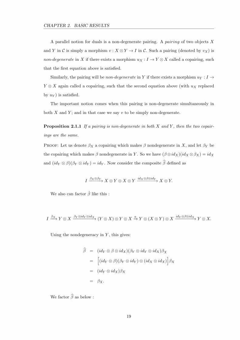
Proposition 2.1.1 If a pairing is non-degenerate in both X and Y , then the two copair-
ings are the same.
Proof: Let us denote βX a copairing which makes β nondegenerate in X, and let βY be
the copairing which makes β nondegenerate in Y . So we have (β⊗ idX)(idX ⊗βX) = idX
and (idY ⊗ β)(βY ⊗ idY ) = idY . Now consider the composite β defined as
IβX⊗βY−−−−−→ X ⊗ Y ⊗X ⊗ Y idX⊗β⊗idY−−−−−−−→ X ⊗ Y.
We also can factor β like this :
IβX−−→ Y ⊗X βY ⊗idY ⊗idX−−−−−−−−→ (Y ⊗X)⊗ Y ⊗X a−→ Y ⊗ (X ⊗ Y )⊗X idY ⊗β⊗idX−−−−−−−→ Y ⊗X.
Using the nondegeneracy in Y , this gives:
β = (idY ⊗ β ⊗ idX)(βY ⊗ idY ⊗ idX)βX
=[(idY ⊗ β)(βY ⊗ idY )⊗ (idX ⊗ idX)
]βX
= (idY ⊗ idX)βX
= βX .
We factor β as below :
19
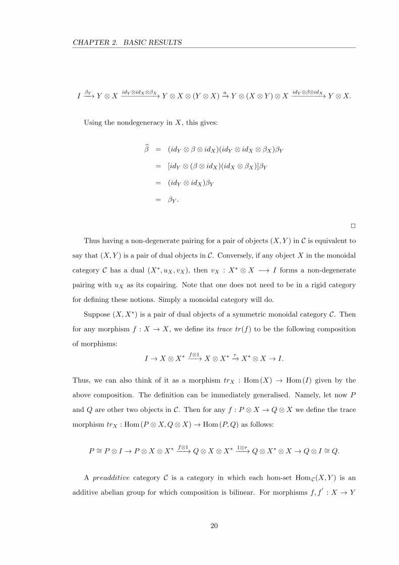
CHAPTER 2. BASIC RESULTS
IβY−−→ Y ⊗X idY ⊗idX⊗βX−−−−−−−−→ Y ⊗X ⊗ (Y ⊗X)
a−→ Y ⊗ (X ⊗ Y )⊗X idY ⊗β⊗idX−−−−−−−→ Y ⊗X.
Using the nondegeneracy in X, this gives:
β = (idY ⊗ β ⊗ idX)(idY ⊗ idX ⊗ βX)βY
= [idY ⊗ (β ⊗ idX)(idX ⊗ βX)]βY
= (idY ⊗ idX)βY
= βY .
2
Thus having a non-degenerate pairing for a pair of objects (X,Y ) in C is equivalent to
say that (X,Y ) is a pair of dual objects in C. Conversely, if any object X in the monoidal
category C has a dual (X∗, uX , vX), then vX : X∗ ⊗ X −→ I forms a non-degenerate
pairing with uX as its copairing. Note that one does not need to be in a rigid category
for defining these notions. Simply a monoidal category will do.
Suppose (X,X∗) is a pair of dual objects of a symmetric monoidal category C. Then
for any morphism f : X → X, we define its trace tr(f) to be the following composition
of morphisms:
I → X ⊗X∗ f⊗1−−→ X ⊗X∗ τ−→ X∗ ⊗X → I.
Thus, we can also think of it as a morphism trX : Hom(X) → Hom(I) given by the
above composition. The definition can be immediately generalised. Namely, let now P
and Q are other two objects in C. Then for any f : P ⊗X → Q⊗X we define the trace
morphism trX : Hom(P ⊗X,Q⊗X)→ Hom(P,Q) as follows:
P ∼= P ⊗ I → P ⊗X ⊗X∗ f⊗1−−→ Q⊗X ⊗X∗ 1⊗τ−−→ Q⊗X∗ ⊗X → Q⊗ I ∼= Q.
A preadditive category C is a category in which each hom-set Hom C(X,Y ) is an
additive abelian group for which composition is bilinear. For morphisms f, f′
: X → Y
20
CHAPTER 2. BASIC RESULTS
and g, g′
: Y → Z,
(g + g′) ◦ (f + f
′) = g ◦ f + g ◦ f ′ + g
′ ◦ f + g′ ◦ f ′ .
Thus, Ab, R-Mod, Mod-R are preadditive categories. A preadditive category is called
additive if the following conditions are satisfied:
(i) There is a zero object 0 ∈ Ob C such that Hom C(0, X) = Hom C(X, 0) = 0 for all
X ∈ Ob C.
(ii) Every finite set of objects has a product. This means that we can form finite direct
products.
If C and D are preadditive categories, an additive functor T : C → D is a functor from
C to D with
T (f + f′) = Tf + Tf
′.
for any parallel pair of arrows f, f′
: X → Y in C.
Let C and D be categories and let T : C → D and S : D → C be covariant functors. T
is said to be a left adjoint functor to S (equivalently, S is a right adjoint functor to T ) if
there is a natural isomorphism :
ν : HomD(T (−),−)·−→ Hom C(−, S(−)).
Here the functor HomD(T (−),−) is a bifunctor C × D → Set which is contravariant
in the first variable, is covariant in the second variable, and sends an object (C,D) to
HomD(T (C), D). The functor HomC(−, S(−)) is defined analogously. Essentially, it says
that for every object C in C and every object D in D there is a function
νC,D : HomD(T (C), D)∼−→ HomC(C, S(D))
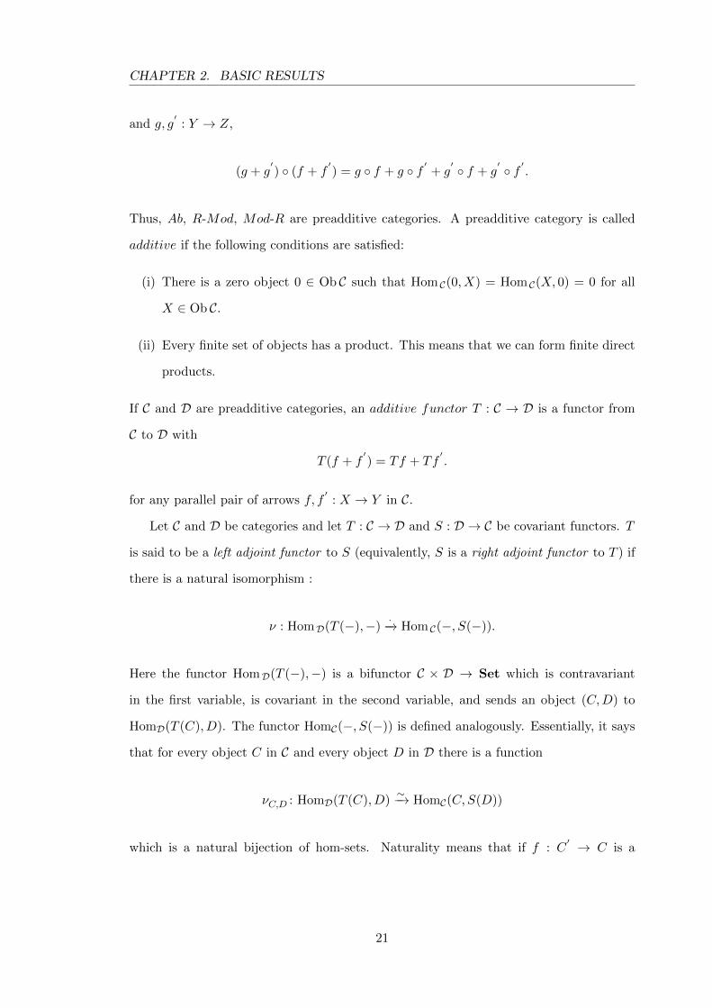
which is a natural bijection of hom-sets. Naturality means that if f : C′ → C is a
21
CHAPTER 2. BASIC RESULTS
morphism in C and g : D → D′
is a morphism in D, then the following diagram:
HomD(T (C), D
)(Tf,g)
��
νC,D // HomC(C, S(D)
)(f,Sg)
��HomD
(T (C
′), D
′) νC′,D′
// HomC(C′, S(D
′)).
commutes. If we pick any h : T (C)→ D, then we have the equation
Sg ◦ νC,D(h) ◦ f = νC′ ,D′
(g ◦ h ◦ Tf).
If T : C → D is a left adjoint of S : D → C, then we say that the ordered pair (T, S) is an
adjoint pair, and the ordered triple (T, S, ν) an adjunction from C to D, written as
(T, S, ν) : C → D,
where ν is the natural equivalence defined above. An adjoint to any functor is unique up
to natural isomorphism.
Let (C,⊗, IC) and (D,⊗, ID) be monoidal categories. A lax monoidal functor from C
to D consists of a functor F : C → D together with a natural transformation
φA,B : FA⊗FB → F(A⊗B)
and a morphism
φ : ID → FIC ,
called the coherence maps or structure morphisms, which are such that for any three
objects A, B and C of C the diagrams
22
CHAPTER 2. BASIC RESULTS
(FA⊗FB)⊗FC
φA,B⊗1
��
aD // FA⊗ (FB ⊗FC)
1⊗φB,C
��F(A⊗B)⊗FC
φA⊗B,C
��
FA⊗F(B ⊗ C)
φA,B⊗C
��F((A⊗B)⊗ C
) FaC // F(A⊗ (B ⊗ C)
)
(2.1)
FA⊗ ID
ρD
��
1⊗φ // FA⊗FIC
φA,IC
��FA F(A⊗ IC).
FρCoo
ID ⊗FB
λD
��
φ⊗1 // FIC ⊗FB
φC ,B
��FB F(IC ⊗B).
FλCoo
(2.2)
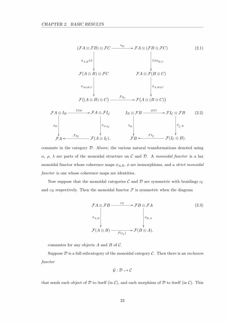
commute in the category D. Above, the various natural transformations denoted using
α, ρ, λ are parts of the monoidal structure on C and D. A monoidal functor is a lax
monoidal functor whose coherence maps φA,B, φ are isomorphisms, and a strict monoidal
functor is one whose coherence maps are identities.
Now suppose that the monoidal categories C and D are symmetric with braidings cC
and cD respectively. Then the monoidal functor F is symmetric when the diagram
FA⊗FB
φA,B
��
cD // FB ⊗FA
φB,A
��F(A⊗B)
F(cC)// F(B ⊗A).
(2.3)
commutes for any objects A and B of C.
Suppose D is a full subcategory of the monoidal category C. Then there is an inclusion
functor
G : D ↪→ C
that sends each object of D to itself (in C), and each morphism of D to itself (in C). This
23
CHAPTER 2. BASIC RESULTS
functor is a faithful functor. In addition, if D is a monoidal subcategory of C, then D
is closed under the tensor product of objects and morphisms and contains the identity
object of C. Thus ID = IC = I, say. Let
F : C → D
be a functor such that there is a natural isomorphism θ : 1→ GF , θA : A 7→ FA. Then,
C and D are equivalent categories. We want to investigate whether the equivalence of
monoidal categories a monoidal equivalence. The answer is negative in general and the
equivalent monoidal categories C and D need not possess monoidal equivalence.
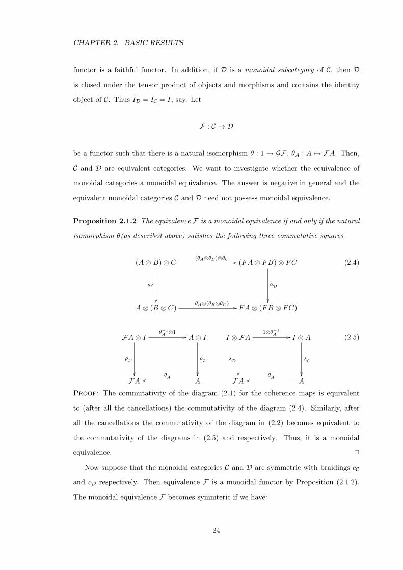
Proposition 2.1.2 The equivalence F is a monoidal equivalence if and only if the natural
isomorphism θ(as described above) satisfies the following three commutative squares
(A⊗B)⊗ C
aC
��
(θA⊗θB)⊗θC // (FA⊗ FB)⊗ FC
aD
��A⊗ (B ⊗ C)
θA⊗(θB⊗θC) // FA⊗ (FB ⊗ FC)
(2.4)
FA⊗ I
ρD
��
θ−1A ⊗1
// A⊗ I
ρC
��FA A
θAoo
I ⊗FA
λD
��
1⊗θ−1A // I ⊗A
λC
��FA A
θAoo
(2.5)
Proof: The commutativity of the diagram (2.1) for the coherence maps is equivalent
to (after all the cancellations) the commutativity of the diagram (2.4). Similarly, after
all the cancellations the commutativity of the diagram in (2.2) becomes equivalent to
the commutativity of the diagrams in (2.5) and respectively. Thus, it is a monoidal
equivalence. 2
Now suppose that the monoidal categories C and D are symmetric with braidings cC
and cD respectively. Then equivalence F is a monoidal functor by Proposition (2.1.2).
The monoidal equivalence F becomes symmteric if we have:
24
CHAPTER 2. BASIC RESULTS
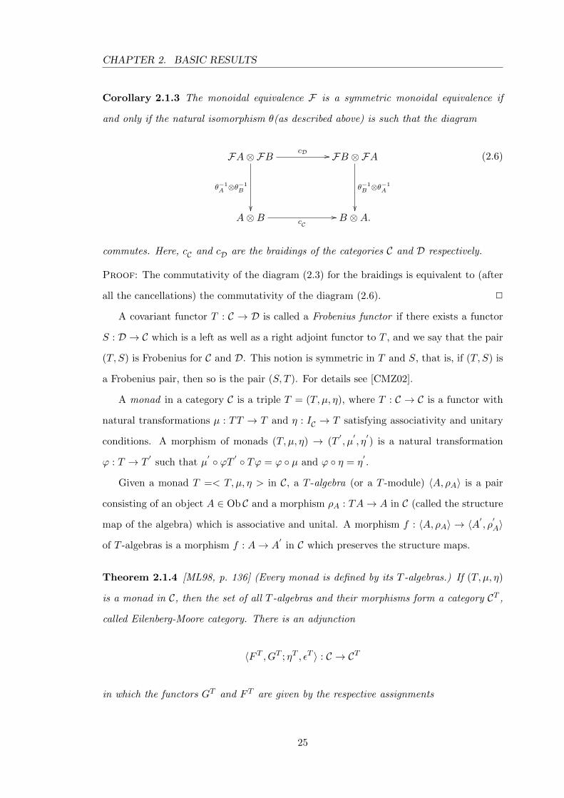
Corollary 2.1.3 The monoidal equivalence F is a symmetric monoidal equivalence if
and only if the natural isomorphism θ(as described above) is such that the diagram
FA⊗FB
θ−1A ⊗θ
−1B
��
cD // FB ⊗FA
θ−1B ⊗θ
−1A
��A⊗B cC
// B ⊗A.
(2.6)
commutes. Here, cC and cD are the braidings of the categories C and D respectively.
Proof: The commutativity of the diagram (2.3) for the braidings is equivalent to (after
all the cancellations) the commutativity of the diagram (2.6). 2
A covariant functor T : C → D is called a Frobenius functor if there exists a functor
S : D → C which is a left as well as a right adjoint functor to T , and we say that the pair
(T, S) is Frobenius for C and D. This notion is symmetric in T and S, that is, if (T, S) is
a Frobenius pair, then so is the pair (S, T ). For details see [CMZ02].
A monad in a category C is a triple T = (T, µ, η), where T : C → C is a functor with
natural transformations µ : TT → T and η : IC → T satisfying associativity and unitary
conditions. A morphism of monads (T, µ, η) → (T′, µ′, η′) is a natural transformation
ϕ : T → T′
such that µ′ ◦ ϕT ′ ◦ Tϕ = ϕ ◦ µ and ϕ ◦ η = η
′.
Given a monad T =< T, µ, η > in C, a T -algebra (or a T -module) 〈A, ρA〉 is a pair
consisting of an object A ∈ Ob C and a morphism ρA : TA→ A in C (called the structure
map of the algebra) which is associative and unital. A morphism f : 〈A, ρA〉 → 〈A′, ρ′A〉
of T -algebras is a morphism f : A→ A′
in C which preserves the structure maps.
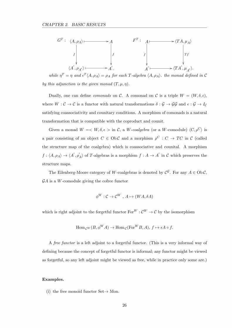
Theorem 2.1.4 [ML98, p. 136] (Every monad is defined by its T -algebras.) If (T, µ, η)
is a monad in C, then the set of all T -algebras and their morphisms form a category CT ,
called Eilenberg-Moore category. There is an adjunction
〈F T , GT ; ηT , εT 〉 : C → CT
in which the functors GT and F T are given by the respective assignments
25
CHAPTER 2. BASIC RESULTS
GT : 〈A, ρA〉
f
��
� // A
f
��〈A′ , ρA′ 〉
� // A′.
F T : A
f
��
� // 〈TA, µA〉
Tf
��
A′ � // 〈TA′ , µ
A′〉.
while ηT = η and εT 〈A, ρA〉 = ρA for each T -algebra 〈A, ρA〉. the monad defined in C
by this adjunction is the given monad (T, µ, η).
Dually, one can define comonads on C. A comonad on C is a triple W = (W, δ, ε),
where W : C → C is a functor with natural transformations δ : G → GG and ε : G → IC
satisfying coassociativity and counitary conditions. A morphism of comonads is a natural
transformation that is compatible with the coproduct and counit.
Given a monad W =< W, δ, ε > in C, a W -coalgebra (or a W -comodule) 〈C, ρC〉 is
a pair consisting of an object C ∈ Ob C and a morphism ρC : C → TC in C (called
the structure map of the coalgebra) which is coassociative and counital. A morphism
f : 〈A, ρA〉 → 〈A′, ρ′A〉 of T -algebras is a morphism f : A → A
′in C which preserves the
structure maps.
The Eilenberg-Moore category of W -coalgebras is denoted by CG . For any A ∈ Ob C,
GA is a W -comodule giving the cofree functor
φW : C → CW , A 7→ (WA, δA)
which is right adjoint to the forgetful functor ForW : CW → C by the isomorphism
Hom CW (B,φWA)→ Hom C(ForWB,A), f 7→ εA ◦ f.
A free functor is a left adjoint to a forgetful functor. (This is a very informal way of
defining because the concept of forgetful functor is informal; any functor might be viewed
as forgetful, so any left adjoint might be viewed as free, while in practice only some are.)
Examples.
(i) the free monoid functor Set→ Mon.
26
CHAPTER 2. BASIC RESULTS
(ii) the free module functor Set→ K-Mod for a ring K.
(iii) the free group functor Set→ Grp.
A very important example (concept) forming a free functor is the left adjoint C → CF ,
where F is a monad on the category C and CF is its Eilenberg-Moore category. This
includes all of the three examples above.
2.2 Crossed modules
Crossed modules were first introduced by J. H. C. Whitehead as a tool for homotopy
theory. They also occur naturally in many other situations (see examples below).
Definition 2.2.1 A crossed module H = (H,π, t, ϕ) consists of groups H, π together
with a group homomorphism t : H → π and a left action ϕ : π ×H → H on H, written
as αh := ϕ(α, h), satisfying the conditions
CM1 t(αh) = αt(h)α−1
CM2 t(h)h′
= hh′h−1.
When the action is unambiguous, we may writeH as a triple (H,π, t). The two crossed
module axioms also have names, which are inconsistently applied. CM1 is sometimes
known as equivariance; CM2 is called the Peiffer identity. A structure with the same
data as a crossed module and satisfying the equivariance condition but not the Peiffer
identity is called a precrossed module.
Examples. Certain generic situations give rise to crossed modules. Some are detailed
here.
(i) Suppose N C G is a normal subgroup. Then G acts on N by conjugation; this
action and the inclusion i : N ↪→ G form a conjugation crossed module, (N,G, i).
(ii) If M is a G-module, there is a well-defined G-action on M . This together with the
zero homomorphism : M → G (sending everything in M to the identity in G) yields
a G-module crossed module, (M,G, 0).
27
CHAPTER 2. BASIC RESULTS
(iii) Let G be any group and Aut(G) its group of automorphisms. There is an obvious
action of Aut(G) on G, and a homomorphism φ : G→ Aut(G) sending each g ∈ G to
the inner automorphism of conjugation by g. These together form an automorphism
crossed module, (G,Aut(G), φ).
(iv) Any group G may be thought of as a crossed module in two ways. Since G always has
the two normal subgroups {1} and G, we can form the conjugation crossed modules
{1} ↪→ G and id : G→ G. Note that the homomorphism G→ {1} with the trivial
action forms a crossed module whenever G is abelian, otherwise the Peiffer identity
fails and the result is a precrossed module.
2.3 Cohomology of groups
Let G be a multiplicative group. Suppose M is an abelian group. Then M can be
regarded as a trivial G-module (via the action xµ = µ for x ∈ G, µ ∈ M) and the
cohomology groups Hn(G,M) can be constructed.
For n ≥ 0, let Cn(G,M) be the group of all functions from Gn to M . This is an
abelian group; its elements are called the (inhomogeneous) n-cochains. The coboundary
homomorphisms
dn : Cn(G,M)→ Cn+1(G,M)
are defined as
(dnϕ) (g1, . . . , gn+1) = ϕ(g2, . . . , gn+1) +n∑i=1
(−1)iϕ(g1, . . . , gi−1, gigi+1, gi+2, . . . , gn+1
)(−1)n+1ϕ
(g1, . . . , gn
).
The crucial thing to check here is
dn+1 ◦ dn = 0.
Thus we have a cochain complex and we can compute cohomology. For n ≥ 0, define the
28
CHAPTER 2. BASIC RESULTS
group of n-cocycles as: Zn(G,M) = ker(dn) and the group of n-coboundaries as
Bn(G,M) =
0 ; n = 0
im(dn−1) ; n ≥ 1
and finally the cohomology group of G with coefficients in M is defined as
Hn(G,M) = Zn(G,M)/Bn(G,M).
Let θ be a 2-cocycle of G. This implies θ ∈ Z2(G,M). Then d2(θ) = 0. Thus for any
f, g, h ∈ G using the definition of the differential d2, we get
θ(f, gh) + θ(g, h) = θ(f, g) + θ(fg, h) (2.7)
A 2-cocycle θ of G is called normalised if
θ(f, 1) = θ(1, g) = 0. (2.8)
Further, a 3-cochain σ of G is a coboundary of θ implies that dθ = σ. Thus we have:
σ(f, g, h) + θ(f, gh) + θ(g, h) = θ(f, g) + θ(fg, h) (2.9)
Suppose σ is a 3-cocycle of G. This implies σ ∈ Z3(G,M). Then d3(σ) = 0. Thus for any
a, b, c, d ∈ G using the definition of the differential, we get
σ(a, b, c) + σ(d, ab, c) + σ(d, a, b) = σ(d, a, bc) + σ(da, b, c)
A 3-cocycle σ is called normalised if
σ(f, 1, h) = 0.
29
CHAPTER 2. BASIC RESULTS
Suppose G = Z, then we have
H0(G,M) = M
H i(G,M) = 0 for i ≥ 1.
In particular, H3(Z,M) = 1 since Z is a projective Z-module, where as for any cyclic
group of order n, H3(Zn,M) = nM where nM ={µ ∈ M
∣∣nµ = 0}
, and a standard
3-cocycle that gives the cohomology class of µ ∈ nM is given by the standard formula:
σ(x, y, z) =
0 ; y + z < n
xnµ ; y + z ≥ n
for some µ ∈ nM .
2.4 Duality and Pairings
Suppose S is a commutative ring with unity. Let A be an S-algebra. We say that
an ideal I of A is finite coprojective if A/I is finitely generated projective S-module. We
define a finite dual A◦ of A to be the S-algebra given by
A◦ = {f ∈ A∗∣∣f(I) = 0 ; I is finite coprojective.} (2.10)
Now consider two Hopf algebras A and B (over K). A Hopf Pairing between them is
a bilinear pairing σ : A×B → K such that, for all a, a′ ∈ A and b, b
′ ∈ B,
σ(a, bb′) = σ(a(1), b)σ(a(2), b
′), (2.11)
σ(aa′, b) = σ(a, b(2))σ(a
′, b(1)), (2.12)
σ(a, 1) = ε(a) and σ(1, b) = ε(b) (2.13)
Note that such a pairing always verifies that, for any a ∈ A and b ∈ B,
σ(S(a), S(b)) = σ(a, b), (2.14)
30
CHAPTER 2. BASIC RESULTS
since both σ and σ(S ⊗ S) are the inverse of σ(id ⊗ S) in the algebra HomK(A ⊗ B,K)
endowed with the convolution product.
2.5 Schemes
Let K be a commutative ring. An affine scheme X over K is a locally ringed space
(X,OX) such that its base space X is isomorphic to SpecR for some commutative K-
algebra R. If x ∈ R, define the basic open set Xx = {p ∈ SpecR : x /∈ p}. It is the
locus where x does not vanish. Then {Xx}x∈R forms a prebasis of X and equips X with
a Zariski topology.
Consider the multiplicative subset S = R − p, where p is a prime ideal of R. The
localisation S−1R is denoted by Rp. For a non zero x in R, the localisation of the
multiplicative subset {1, x, x2, · · · } denoted by Rx is just the ring obtained by inverting
powers of x. Note if x is nilpotent, the localisation is the zero ring. (Note : If (x) is a
prime ideal, then Rx 6= R(x) .) Here is an example: R = C[X,Y ], x = X. In this case
RX = C[X,X−1, Y ]. On the other hand every nonzero element of R(X) = {R\(X)}−1R
has a unique representation Xnu, where u is a fraction, such that X is coprime to both
the numerator and the denominator of u. We can call this ring the local ring of the affine
plane at the line X = 0 ı.e. R(X) is the ring of rational functions on C2 which do not
have a pole along the hyperplane X = 0.
A scheme X over K is a locally ringed space (X,OX) admitting an open covering
{Ui}i∈I , such that for each i, (Ui,OX |Ui) is isomorphic as locally ringed space to an affine
scheme over K . Points of X are referred to as topological points of X or Xtop. A
morphism of schemes is a morphism of locally ringed spaces. An isomorphism will be a
morphism with two-sided inverse. Indeed, schemes form a category, Sch. Morphisms from
schemes to affine schemes are completely understood in terms of ring homomorphisms by
the following contravariant adjoint pair: For any scheme X and a commutative K-algebra
R we have a natural equivalence
MorSch(X ,SpecR) ∼= MorK−Alg
(R,OX(X)
),
31
CHAPTER 2. BASIC RESULTS
where K−Alg is the category of commutative K-algebras. Since K is an initial object
in the category K−Alg, the category of schemes has Spec (K) as a final object.
The category of schemes has finite products. By definition, the product of X and Y in
the category is the unique object satisfying the universal property that if Z is any object
in Schemes with maps to X and Y, then both maps factor uniquely through a map from
Z → X × Y. A generalisation of this notion is that of the fiber product. Let now X and
Y be be schemes over a base scheme S. This means both X and Y are equipped with
some specified scheme morphisms to the base scheme S. Then any object Z with maps
to both X and Y commuting with these specified maps factors uniquely through the fiber
product of X and Y, denoted as X ×S Y.
Before we construct the fiber product for arbitrary schemes, let us take a look at
the case that X , Y, and S are all affine. We know that the category of affine schemes is
equivalent to the category of commutative rings, with all the arrows reversed. So, in order
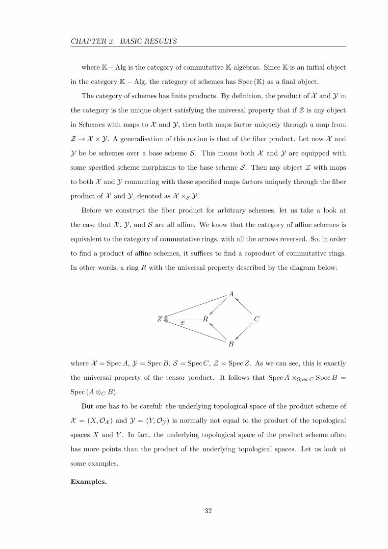
to find a product of affine schemes, it suffices to find a coproduct of commutative rings.
In other words, a ring R with the universal property described by the diagram below:
A
��~~~~~~~~
uujjjjjjjjjjjjjjjjjjjjj
Z R∃!oo C
``@@@@@@@@
��~~~~~~~~
B
iiTTTTTTTTTTTTTTTTTTTTT
__@@@@@@@@
where X = SpecA, Y = SpecB, S = SpecC, Z = SpecZ. As we can see, this is exactly
the universal property of the tensor product. It follows that SpecA ×SpecC SpecB =
Spec (A⊗C B).
But one has to be careful: the underlying topological space of the product scheme of
X = (X,OX ) and Y = (Y,OY) is normally not equal to the product of the topological
spaces X and Y . In fact, the underlying topological space of the product scheme often
has more points than the product of the underlying topological spaces. Let us look at
some examples.
Examples.
32
CHAPTER 2. BASIC RESULTS
(i) If K is the field with nine elements, then SpecK × SpecK ≈ Spec (K ⊗Z K) ≈
Spec (K⊗Z3 K) ≈ Spec (K×K), a set with two elements, though SpecK has only a
single element.
(ii) If K is algebraically closed, then as a set for closed points, A2 = A1 × A1. Observe
the following: A1 ×SpecK A1 = SpecK[x]×SpecK SpecK[y] = Spec (K[x]⊗K K[y]) =
SpecK[x, y] = A2. Thus the product of the closed points of A1 with itself is A2
considered as a set. But note that the underlying topological space of A2 is not
the product topology of the underlying topological space of A1 with itself. The
product topology on A2 is the finite complement topology but the topology on A2
is different.
(iii) Another important example of a fiber product is the case where f : X → S is a
morphism, and α is a point in S. Then consider X ×S α. If X and S were sets,
this would be the set of points of X whose image in S is α. In other words, the
preimage or fiber of α. From this perspective, we can think of f : X → S as a family
of schemes parametrised by S, where the member of the family corresponding to a
point α in S is the fiber of f over α.
So far we have looked at the fiber product of affine schemes. We ought to construct
the fiber product of arbitrary schemes. Since we have already done the affine case, we just
need to patch the local products together to get some sort of global product. Moreover,
notice that since the fiber product satisfies a universal property, it is unique up to unique
isomorphism. This uniqueness is important for proving the following result also discussed
by Hartshorne [Har77] :
Theorem 2.5.1 For any X , Y schemes over S, the fiber product X ×S Y exists.
Suppose X is a scheme, and R is a commutative K-algebra. If for all non-empty open
sets U , the sections Γ(U,OX) are R-algebras and the restrictions are R-algebra maps,
then we say that X is an R−scheme, or a scheme over R. We also have an equivalence
of the category of K−schemes with a full sub category of the category of functors from
commutative K-algebras to Sets. So we think of an affine K−scheme X = (X,OX) where
X = SpecR as a functor such that for any K-algebra A, X(A) := HomK(R,A) as a set
33
CHAPTER 2. BASIC RESULTS
or equivalently X(A) := MorSch(SpecA,X). Thus points of X are now referred to as
points of X corresponding to A, or A−points. If A is not specified, we simply call them
algebraic points of X. Note that points must be K-linear.
If X =⋃i(Ui,OUi), such that for each i, Ui ∼= SpecRi and Ui ∩ Uj = SpecRij with
Riαij−−→ Rij . Define X(A) =
⋃i Ui(A)
/∼ where (xi : Ri → A) ∼ (xj : Rj → A) if and
only if either i = j or xi|Rij = xj |Rij .
A scheme X = (X,OX) is said to be locally of finite type over K if corresponding to
an open covering {Ui}i∈I of X, each (Ui,OX |Ui) is isomorphic as locally ringed space to
(Spec (Ri),ORi), where Ri’s are finitely generated algebras over K. A scheme is said to
be of finite type over K if it is a scheme locally of finite type over K, and the open cover
is taken as finite. A scheme of finite type over K is affine if the open cover can consist
of precisely one open set. This means (X,OX) is isomorphic as a ringed space over K,
to (SpecR,OR) for some finitely generated K-algebra R. A scheme (X,OX) is said to
be reduced if for every open subset U ∈ X, the ring OX(U) has no non-zero nilpotent
elements.
Before we describe group schemes overK, we discuss diagonal and structure morphisms
of a scheme (X,OX) over K.
For each affine open subset U = Spec (R) of a scheme X = (X,OX), let φR be
the canonical injection of K into R. Then φR define a morphism fR of (SpecR,OR) to
(SpecK,OK). These fR’s define a morphism πX : (X,OX) → (SpecK,OK), which is
called the structure morphism of X .
The diagonal morphism ∆X is the unique morphism of X to X×X such that p1·∆X =
p2 ·∆X = 1X , where p1 and p2 are the projections of X × X to the first and the second
factors of X ×X respectively.
Let G = (G,OG) be a scheme over K. Then we say that (G,OG, µ) is a group
scheme over K if it satisfies the following conditions: (1) µ : G × G → G is such that
µ(1G × µ) = µ(µ × 1G); (2) there exists an endomorphism γ of G and a morphism ε of
SpecR to G such that µ(1G × γ)∆G = µ(γ × 1G)∆G = ε · πG, where ∆G and πG are the
diagonal and the structure morphism ofG respectively; and (3) µ(ε×1G) = µ(1G×ε) = 1G,
where we identify Spec(k) × G and G × Spec(k) with G canonically. The morphisms µ,
34
CHAPTER 2. BASIC RESULTS
ε and γ are called the multiplication, the identity morphism and the inverse morphism
of G respectively, and the image e of ε in G is called the neutral point of G. We denote
a group scheme as (G,µ, ε, γ). For example, GLn can be defined as the affine scheme of
invertible integral n× n matrices, SpecZ[xij ][det(xij)−1].
Define Mor(X,G) as the set of all scheme-morphisms from the scheme (X,OX) over
K to the group scheme (G,OG, µ) over K. Then Mor(X,G) forms a group under the
composition f ∗ g = µ(f × g)∆X for f, g ∈ Mor(X,G). Note that the base space G of
a group scheme (G,OG, µ) over K is not a group in general. Consider for example the
polynomial ring R = R[x], G = SpecR which gives the additive group scheme Ra whereas
its topological points or its closed points: G = {(0), (x− a), (x− z)(x− z); a ∈ R, z ∈ C}
fail to form a group!
If R is a commutative ring, then we have an equivalence of the category of R-group
schemes with a full sub category of the category of functors from R-algebras to Groups.
So we can also think of an R-group scheme (G,OG) as a functor on R-algebras where
G(A) = Mor(Spec (A), G) is a group for any R-algebra, A.
Examples. For any commutative K-algebra A, consider the following examples of a
group scheme G as a functor on the category of K-algebras,
(i) For a discrete group G, the constant functor G(A) = G defines a group scheme. The
topological space is the topological group G and Op = K.
(ii) If H is a finitely generated commutative Hopf Algebra, the group scheme G takes
A to the group of algebra morphisms from H to A. Here the topological space is
SpecH and G(A) = Hom(H,A).
(iii) The group scheme G = GLn associates to every K-algebra A, the group GLn(A).
(iv) Cn/Z2n is a group scheme over C.
2.5.1 Algebraic Groups
An affine algebraic group is an affine reduced group scheme G over algebraically closed
field K equipped with morphisms of varieties µ : G × G → G, i : G → G that give G
the structure of a group. A morphism f : G → H of algebraic groups is a morphism of
varieties that is a group homomorphism too.
35
CHAPTER 2. BASIC RESULTS
Examples. (i) The additive group Ga ı.e. the affine variety A1 under addition. (ii) The
multiplicative group Gm ı.e. the principal open subset A1\{0} under multiplication. (iii)
The group GLn = GLn(k) of all invertible n × n matrices over K. As a variety this is
a principal open set in Mn(K) = An2corresponding to the determinant. (iv) The group
SLn = SLn(K) is the closed subgroup of GLn defined by the zeros of det−1.
Let G be an (affine) algebraic group with the identity element e. Let H = K[G]. Then
the map
ε : H → k, f 7→ f(e)
is an algebra homomorphism (called augmentation). Consider also the dual morphisms
∆ := µ∗ : H → H ⊗H
(called comultiplication) and
σ := i∗ : H → H
(called antipode ). It follows using the group axioms that these define the structure of
a Hopf algebra on K[G]. Conversely, a structure of the Hopf algebra on K[G] defines a
structure of an algebraic group on G. Infact, we have the following known fact:
Theorem 2.5.2 The categories of (affine) algebraic groups and affine Hopf algebras are
contravariantly equivalent.
Note that group schemes generalise algebraic groups, in the sense that all algebraic
groups have a group scheme structure, but group schemes are not necessarily connected,
smooth, or defined over a field. Infact, an algebraic group is a reduced group scheme
over an algebraically closed field. For convenience we shall set following identification
for the thesis: G = G(K), where G on the right side is a reduced group scheme over an
algebraically closed field K, so that G(K) is a group. Moreover, G on the left side will be
an algebraic group inheriting the variety structure from the group scheme G.
36
CHAPTER 2. BASIC RESULTS
2.6 Sheaves
Let (X,OX) be an affine scheme with X = SpecR, and a commutative ring R. Sup-
pose M is an R-module. We defineM as a sheaf on the basic open set Xx of X as follows.
To every x ∈ X and the corresponding basic open set Xx, we associate Mx = M ⊗R Rx
; the restriction map is the obvious one. Then M is a sheaf of OSpecR -modules. Let F
be a sheaf of OX -modules on X. Then F is
(i) finitely generated(f.g.)/finite type if every point x ∈ X has an open neighbourhood
U such that there is a surjective morphism
OnX |U → F|U
where n ∈ N.
(ii) finitely presented (f.p.) sheaf if there is an exact sequence of the form
OpX |U → OnX |U → F|U → 0
where p, n ∈ N.
Note. Every f.p. OX -module is f.g.
(iii) quasi-coherent sheaf if for every affine open SpecR,
F|SpecR∼= ˜Γ(SpecR,F).
(The wide tilde is supposed to cover the entire right side Γ(SpecR,F). This iso-
morphism SpecR is as sheaves of OX -modules. If F is a quasi-coherent sheaf, then
F is locally a cokernel of a morphism of free-modules. This means there is an open
cover {Uα}α∈Λ of X such that for every α there exist Iα and Jα (not necessarily
finite) and an exact sequence of sheaves of OX -modules of the form:
OIαX |Uα → OJαX |Uα → F|Uα → 0.
37
CHAPTER 2. BASIC RESULTS
(iv) coherent if
• it is finitely generated,
• for any open set U of X, every morphism Op|U → F|U of OX -modules has a
finitely generated kernel, where p ∈ N.
Note that if F is locally finite then the condition of finite generation implies coher-
ence and the other way also.
2.6.1 Tensor product
We first discuss the tensor product of sheaves which are defined on the same scheme.
Suppose X = (X,OX) is a scheme and F , G be sheaves on X . Then the (internal)tensor
product of F and G over X is a sheaf F ⊗X G (or simply F ⊗ G) on X such that the
section of the sheaf at any affine open set U = Spec (R) is defined as F(U)⊗R G(U). In
general, if F and G are any two OX -modules, we define the tensor product F ⊗OX G to be
the sheaf associated to the presheaf U 7→ F(U)⊗OX (U) G(U). This is also an OX -module.
We now describe external tensor product of sheaves which are defined on different
schemes. Let X = (X,OX) and Y = (Y,OY ) be schemes. Suppose F and G are sheaves
respectively on X and Y. We want to construct a sheaf F�G on the product space X ×Y.
Let π1 : X × Y → X and π2 : X × Y → Y be the projection maps of schemes. Then
external tensor product of F and G is the normal tensor product of the pullback sheaves
π∗1F and π∗2G. Note that this yields a sheaf on X × Y. On stalks, there is a canonical
bijection (F � G)(x,y) → Fx � Gy. In particular, you see that if F and G are the sheaves
of K-valued continuous functions on X resp. Y , then F � G is a rather small subsheaf of
the continuous functions on X × Y .
Suppose G is a group scheme and A is a sheaf on G. Then there are three maps from
G × G to G namely, the multiplication, the first projection π1, and the second projection
π2,
µ, π1, π2 : G × G → G.
Let us denote the global sections of A as
Γ := Γ(G,A) = A(G).
38
CHAPTER 2. BASIC RESULTS
Then we have the following result, which we use in the last section of Chapter 4.
Lemma 2.6.1 Suppose A is a sheaf over a scheme G. If A is generated by global sections
Γ, then A�A is generated by Γ× Γ.
Proof: Suppose A is generated by global sections. Then, the natural map
Γ⊗OG −→ A
is a surjection. Now, since pullbacks are right exact, we have the following surjection
π∗1(Γ⊗OG) = Γ⊗ π∗1OG = Γ⊗OG×G −→ π∗1A. (2.15)
Taking tensor product is also right exact, so tensoring with π∗2A, (2.15) gives
f : Γ⊗ π∗2A = Γ⊗OG×G ⊗ π∗2A −→ π∗1A⊗ π∗2A = A�A.
Finally, taking tensor product with Γ, (2.15) gives the following surjection
g : Γ⊗ Γ⊗OG×G −→ Γ⊗ π∗2A.
Composing the last two maps, we get the required surjection
h = fg : Γ⊗ Γ⊗OG×G → A�A.
which makes A�A being generated by Γ⊗ Γ. 2
2.6.2 G-equivariant sheaves
Let G be a group scheme. Let X be a G-scheme ı.e. a scheme equipped with an
algebraic G-action, a : G ×X → X. Thus there are two natural maps
G ×Xa //p
// X
where p is the projection map and a is the action of G on X. A sheaf F of OX -modules on
an algebraic G-variety X is called G-equivariant if the following conditions hold. [CG97].
39
CHAPTER 2. BASIC RESULTS
(a) There is a given isomorphism of sheaves on G ×X
I : a∗F ∼ // p∗F
(b) The pullbacks by id×a and m× id of the isomorphism I are related by the equation
p∗23I ◦ (idG × a)∗I = (m× idX)∗I, where p23 : G × G ×X → G ×X is the projection
along the first factor G.
(c) For e = the unit of G, we have
Ie×X = id : F = a∗F|e×X ∼ // p∗F|e×X = F
Remark. (i) For any G-variety X, the sheaf OX has canonical G-equivariant structure
given by the composition of the following natural isomorphisms: p∗OX ' OG×X ' a∗OX .
(ii) Condition (c) in the definition above is superfluous and is only given for conve-
nience. Indeed, it can be deduced from (a) and (b) as follows. Restricting the equality in
(b) to e× e×X, one finds Ie×X ◦ Ie×X = Ie×X . Since Ie×X is an isomorphism, this yields
Ie×X = id.
2.6.3 Cosheaves
Let R denote a ring. Let X be a topological space. A precosheaf C (of R-modules)
on X is a covariant functor from the category of open sets in X and inclusions to the
category of R-modules, [Bre97]. For U ⊆ V the corresponding map C(U) → C(V ) called
corestrictions is denoted by iV,U .
A precosheaf C on X is called a cosheaf if, for every open covering {Uα} of an open
set U ⊆ X, the sequence
⊕<α,β>
C(Uα ∩ Uβ)ϕ−→⊕α
C(Uα)φ−→ C(U) −→ 0
is exact, where ϕ =∑
α iU,Uα and φ = (∑
<α,β> iUα,Uα∩Uβ − iUβ ,Uα∩Uβ ). The following
result states the necessary and sufficient condition for a precosheaf to become a cosheaf.
Proposition 2.6.2 [Bre97] Let C be a precosheaf. Then C is a cosheaf if and only if the
40
CHAPTER 2. BASIC RESULTS
following two conditions are satisfied:
(a) C(U ∩ V )ϕ−→ C(U) ⊕ C(V )
φ−→ C(U ∪ V ) → 0 is exact for all open U and V where
ϕ = (iU,U∩V − iV,U∩V ) and φ = (iU∩V,U + iU∩V,V ).
(b) If {Uα} is directed upwards by inclusion then the natural map lim C(U)→ C(∪αUα)
is an isomorphism.
Let us discuss the local nature of the notion of a cosheaf formulated for any precosheaf
on a topological space X. A precosheaf C on a topological space X is a cosheaf if for any
open set U ⊆ X and any any open covering U = ∪Uα of U , the following two conditions
hold:
(i) For any u ∈ C(U), there exists finitely many uαi ∈ C(Uαi) such that∑iU,Uαi
(uαi) =
u for each Uαi .
(ii) For all uα ∈ C(Uα), such that ϕ(uα) = 0 there exist uαβ ∈ C(Uα ∩ Uβ) such that
φ(uαβ) = uα.
Examples. Let X = {x1, x2} with the discrete topology, ı.e. all subsets are open. We
write Xi = {xi}. We define precosheaves on X as follows.
(i)
C1 : C1(Xi) = Z (1 ≤ i ≤ 2)
C1(X) = Z
iC1U,V = 0 for U 6= V.
Clearly C1 is a precosheaf. But C1 fails to be a cosheaf because condition (i) in the
above definition fails: 2 ∈ C1(X), but there is no u1 in X1 such that iX,X1(u1) = 2
since 2 6= 0.
41
CHAPTER 2. BASIC RESULTS
(ii)
C2 : C2(Xi) = Z (1 ≤ i ≤ 2)
C2(X) = Z
iC2U,V = idZ for V 6= ∅.
Clearly C2 is a precosheaf. Moreover, C2 is also a cosheaf.
(iii)
C3 : C3(Xi) = Z⊕ Z (1 ≤ i ≤ 2)
C3(X) = Z
iC3X,X1= π1 : Z⊕ Z→ Z : (m,n) 7→ m
iC3X,X2= π1 : Z⊕ Z→ Z : (m,n) 7→ n.
Then C3 is a precosheaf. But C3 fails to be a cosheaf because condition (ii) in
the above definition fails: For u1 = (2, 3) ∈ C3(X1), and u2 = (1,−2) ∈ C3(X2),
φ(∑2
i=1 ui) = (iU,U1 + iU,U2)(u1 + u2) = 2 − 2 = 0 but there are no u12, u′12 ∈
C3(X1∩X2) = 0 such that(iX1,∅− iX2,∅
)(u12 +u
′12) = (2, 3) + (1,−2) = (3, 1) since
iX1,∅(x) is a zero map and (3, 1) 6= (0, 0).
Let A be a sheaf over a scheme G. Let us discuss its dual cosheaf denoted by A∗. It
is defined as
A∗ = HomK(A,K).
Then for each open covering {Ui} of U ⊆ G, the sheaf exact sequence of K-modules,
∏i,j
A(Ui ∩ Uj)⇔∏i
A(Ui)←− A(U)←− 0
turns into cosheaf exact sequence of K-modules
⊕i,jA∗(Ui ∩ Uj)⇒ ⊕iA∗(Ui) −→ A∗(U) −→ 0.
42
CHAPTER 2. BASIC RESULTS
Thus A∗ is a cosheaf of K-modules over group scheme G. Let us now discuss the finite
dual of A which is given by
A◦ ={f ∈ A∗
∣∣∣f(I) = 0 for some ideal I of A ; dimKA/I <∞
}. (2.16)
Then for any f ∈ A◦(U) if fM = (A(U) ⇀ f) and Mf = (A(U) ↼ f), we have that
dimK(fM), dimK(Mf ) <∞. Moreover, F factors through fM and Mf , that is,
f : A(U)→ fM → K,
f : A(U)→Mf → K.
Cosections of A◦ are subspaces of the corresponding cosections of A∗. For each inclusion
of open sets U ⊆ V , the corestriction cores◦V,U : A◦(U)→ A◦(V ) is given by the following
sequence
cores◦V,U (f) : A(V )resU,V−−−−→ A(U) −→ fM −→ K,
Thus the corestrictions of the cosheaf A◦ are induced by the restrictions of A∗. This
makes A◦ a subcosheaf of A∗.
Observe that we can think of sheaves and cosheaves in terms of categories in the
following sense:
(i) A sheaf F on a topological space X can be thought of as a contravariant functor from
the category of open sets on X to some abelian category A with infinite products,
such that they satisfy exactness condition in A.
F : OpenXF−→ A.
(ii) A cosheaf C on a topological space X can be thought of as a covariant functor from
the category of open sets on X to an abelian category A with infinite sums, such
that they satisfy exactness condition in A.
C : OpenXC−→ A.
43
CHAPTER 2. BASIC RESULTS
(iii) The dual of a sheaf F becomes a covariant functor G :
G : OpenXF−→ A
D−→ A′
where D : A → A′
is a contravariant exact functor such that D takes sheaves in A
into cosheaves in A, and vice-versa. Since composition of two contravariant functor
is a covariant functor, the dual of a sheaf is a cosheaf.
(iv) If F is a sheaf of vector spaces on a topological space X then the dual of F is a
cosheaf of vector spaces on the same topological space X. Note that dual of a vector
space is a vector space and the dual of a linear map is linear in addition to duality
being exact.
(v) If F is a sheaf on X of finite dimensional K-algebras then the dual sheaf F∗ is a
cosheaf on X of K-coalgebras.
Analogous to the theory of sheaves over a topological space, we have some more
definitions to say for cosheaves. If C is a cosheaf on X, and x ∈ X, then we define costalk
Cx of C at x to be the inverse(projective) limit of the sets C(U) taken over all open sets
U 3 x with respect to the system of map iV,U for U ⊂ V . In the general case, for any
open set U 3 x, there exists a natural homomorphism of groups
iU,x : Cx −→ C(U).
Let x ∈ U ⊆ X and ux ∈ Cx such that iU,x(ux) ∈ C(U). Then for any neighbourhood W
of x such that x ∈W ⊆ U , there exists w ∈ C(W ) such that
iU,x(ux) = iU,W (w).
Note that here w = iW,x(ux). Further, if u ∈ C(U), then there exists finitely many
uxi ∈ Cxi such that∑iU,Uxi (uxi) = u ∀xi ∈ Uxi . Thus for a cosheaf C, the elements of
C(U) can be specified as families {uxi}xi∈Uxi . We shall call elements of C(U) the cosections.
44
CHAPTER 2. BASIC RESULTS
Example. As we have given X the discrete topology,
Cxi = C(Xi) (1 ≤ i ≤ 2)
If C and D are cosheaves on X, a morphism of cosheaves φ : C → D consists of
a morphism of abelian groups φ(U) : C(U) → D(U) for each open set U , such that
whenever V ⊆ U is an inclusion, the diagram
C(V )
iCU,V
��
φ(V ) // D(V )
iDU,V
��C(U)
φ(U) // D(U)
is commutative, where iC and iD are the corestriction maps in C and D respectively. An
isomorphism is morphism which has two sided inverse. Note that a morphism φ : C → D
of precosheaves on X induces a morphism φx : Cx → Dx on the costalks, for any point
x ∈ X.
A subcosheaf of a cosheaf F over X is a cosheaf F ′ such that for every open set U ⊆ X,
F ′(U) is a subgroup of F(U), and the restriction maps of the sheaf F ′ are induced by
those of F . It follows that for any point x in X, the stalk F ′x is a subgroup of F ′ .
Let f : X → Y be a continuous map of toplogical spaces. For any cosheaf F on X, we
define direct image cosheaf f∗F on Y by f∗F(V ) = F(f−1(V )
)for any open set V ⊆ Y .
2.7 Disjoint Union
Let M,N be any two sets. We define their disjoint union as a set containing all the
elements of M and N but now they are all labelled. Explicitly,
M tN =(M × {0}
)∪(N × {1}
)⊆(M ∪N
)× {0, 1}.
Remarks.
45
CHAPTER 2. BASIC RESULTS
(i) Note that M and N are not subsets of their disjoint union. but we certainly have
injective maps M ↪→M tN and N ↪→M tN . These maps simply put the relevant
index on each element, for example x 7−→ (x, 1)
(ii) The way disjoint union is defined, it satisfies the universal property making it the
coproduct in the category of sets.
(iii) Clearly, M tM 6= M and M t ∅ 6= M or ∅ tM 6= M . Moreover, for any M 6= N ,
M t N 6= N t M as for any m ∈ M such that m /∈ N , (m, 0) ∈ M t N but
(m, 0) /∈ N tM . (If N = M , then of course they are the same).
Similarly we can define the disjoint union of n-factors. Note again that (LtM)tN 6=
Lt(MtN) and so on. With the disjoint union defined on sets, (Set,t, ∅) has a symmetric
monoidal structure. The associativity is just a matter of relabelling, and thus there is a
bijection of sets:
a : (L tM) tN ∼−→ L t (M tN)
such that (l, 0, 0) t (m, 0, 1) t (n, 1) 7→ (l, 0) t (m, 1, 0) t (n, 1, 1) for l ∈ L, m ∈ M and
n ∈ N . In fact, we get a whole family of maps : one for each triplet of sets. This family
is natural in the category of sets. The left and right units are defined by the obvious
bijections (x, 1) 7→ x and (x, 0) 7→ x respectively. Again, interchanging the labelling gives
a bijection of sets
cM,N : M tN ∼−→ N tM
called the twist map. We again get a family of maps : one for each pair of sets. This
family is also natural in the category of sets. An important property of the twist map is
cM,N ◦ cN,M = idMtN .
For sets K,L,M,N , consider any pair of morphisms f : K → M and g : L → N . Then
their disjoint union(coproduct) f t g : K t L→M tN is defined as
(x, 0) 7→(f(x), 0
)and (x, 1) 7→
(g(x), 1
)
46
CHAPTER 2. BASIC RESULTS
for any x ∈ K ∪ L. Thus (Set,t, ∅) is a symmetric monoidal category.
2.8 Orientation
For this section, manifold means a compact, topological manifold possibly with bound-
ary.
Theorem 2.8.1 [Spa81] Let M be a connected, n-dimensional manifold. Then Hn(M,∂M ;Z),
the top dimensional homology group of M , is either trivial or isomorphic to Z.
Definition 2.8.2 A connected, n-manifold M is called orientable if its top homology
group is isomorphic to the integers. An orientation of M is a choice of a particular
isomorphism
o : Z→ Hn(M,∂M ;Z)
A fundamental class ofM , denoted by [M ] is a generator of the Z-moduleHn(M,∂M,Z).
Thus a fundamental class of M gives an orientation of M by o(1) = [M ].
Now suppose M is a disconnected n-dimensional manifold with {M(i)} the connected
components of M . An orientation of M is given by a choice of orientations of its connected
components:
Hn(M,∂M ;Z) ∼=⊕i
Hn(M(i), ∂M(i);Z)
so that restriction to each component is an orientation of that component. The funda-
mental class [M ] is given by ([M(i)]), where [M(i)] is the fundamental class of its connected
component M(i).
Suppose M is an n-manifold with a non-empty boundary ∂M . Then ∂M is a compact
(n − 1)-manifold without boundary. Suppose now M is orientable with a non-empty
boundary, then its boundary is also orientable. Let us explain the induced orientation on
the boundary. The theorem below discusses the induced orientation on the boundary of
an n-manifold. The proof has been discussed in [Spa81]:
Theorem 2.8.3 [Spa81] If M is a compact n-manifold with boundary ∂M , then if M is
orientable, so is ∂M , and any fundamental class of M maps to a fundamental class of
47
CHAPTER 2. BASIC RESULTS
∂M under the connecting homomorphism
∂∗ : Hn(M,∂M ;Z)→ Hn−1(∂M ;Z).
Before we discuss orientation for gluing, let us briefly explain gluing of n-manifolds.
Suppose W1 and W2 are any two n-dimensional manifolds with non-empty boundaries:
∂W1 = K1·∪ L
∂W2 = L′ ·∪ K2.
Let ϕ : L → L′
be a homeomorphism of manifolds. Then we can glue W1 and W2
along ϕ. Let f1 : L→W1 and f2 : L′ →W2 be continuous maps. Then,
W = W1 tW2
/ϕ
is defined by taking the disjoint union of W1 and W2 and quotienting out by the equiva-
lence relation given by ϕ: two points w1 ∈W1 and w2 ∈W2 are equivalent in W if there
is a point x ∈ L such that f1(x) = w1 and f2
(ϕ(x)
)= w2. Note that W1tW2 has disjoint
union topology and W gets a quotient topology. Observe that L and L′
are no longer a
boundary of W . Indeed, W is an n-manifold with boundary K1·∪ K2. There are two
natural maps W1 −→W ←−W2. Now suppose W1 and W2 are oriented n-manifolds. We
wish to provide an orientation to W . We formulate the following theorem to express the
orientation on W .
Theorem 2.8.4 Suppose W1, W2 are oriented n-manifolds with boundaries
∂W1 = K·∪ L
∂W2 = L·∪M
such that K ∩ M = ∅ and W = W1 ∪ W2. If L induces opposite orientation when
considered as a boundary of W1 and W2 respectively, then the orientation of W1 and W2
48
CHAPTER 2. BASIC RESULTS
can be extended to provide an orientation on W .
Proof: We do the proof in three easy steps. Firstly, observe that the relative Mayor
Vietoris sequence
· · · → Hn(L,L)→ Hn(W1, ∂W1)⊕Hn(W2, ∂W2)→ Hn(W,K∪L∪M)→ Hn−1(L,L)→ · · ·
for an excisive couple of pairs {(W1, ∂W1), (W2, ∂W2)} yields an isomorphism
Hn(W1, ∂W1)⊕Hn(W2, ∂W2) ∼= Hn(W,K ∪ L ∪M)
since Hn(L,L) = Hn−1(L,L) = 0. Secondly, the excision map
(L, ∅) ⊆ (K ∪ L ∪M,K ∪M)
induces an isomorphism on homology
Hn(L) ∼= Hn(K ∪ L ∪M,K ∪M).
Finally, the inclusion of the pairs
(K ∪ L ∪M,K ∪M) ⊆ (W,K ∪M) ⊆ (W,K ∪ L ∪M)
yield a sequence of homomorphism (all coefficients in Z)
Hn(L)→ Hn(W,∂W )α−→ Hn(W1, ∂W1)⊕Hn(W2, ∂W2)
∂∗−→ Hn−1(L).
Note that Hn(L) = 0 and if [W1] and [W2] are fundamental classes of W1 and W2 respec-
tively, then the given condition implies that ∂∗([W1]+[W2]
)= 0. Then [W1]+[W2] = α(x)
for some x ∈ Hn(W,∂W ). It is easy to show that x is a fundamental class of W . Hence
the orientation of W1 and W2 is extended to provide an orientation on W . 2
49
CHAPTER 2. BASIC RESULTS
2.9 HQFT
Homotopy quantum field theories (HQFTs) were introduced by Turaev, and they are
essentially TQFTs in a background space X, up to homotopy. A modified version with
change to one of the axioms was introduced by Rodrigues, [Rod01]. This gave dependence
of (d+1)-HQFTs over X on the (d+1)-type of X. This was used by Brightwell and Turner,
[BT00], and Turner and Willerton, [BTW02], to look at (1+1)-HQFTs with background
space a simply connected space. Thus the results of [Tur99] had classified (1+1)-HQFTs
with background spaces which were 1-types and the more recent results handled simply
connected spaces, classification results there being in terms of the second homotopy group
of X. Rodrigues showed that an n-dimensional HQFT can be regarded as a monoidal
functor
Z : nCob(X)→ V ect
where nCob(X) is the category whose objects are (n− 1) closed manifolds equipped with
a map into X, and whose morphisms are cobordisms equipped with a map into X, consid-
ered up to homotopy (in X) fixing the boundary. We have adopted the same philosophy,
but we work in topological setup whereas he works with diffeomorphisms of manifolds. In
his setup, he considers diffeomorphisms between manifolds. The morphisms between ob-
jects in his category nCob(X) are essentially strings of cobordisms and diffeomorphisms.
On the other hand, our mechanism shall regard an n-dimensional HQFT as a monoidal
functor
Z : X − Cobn → A
for any monoidal category A. The construction of our category X −Cobn involves going
up to some level of 2-categories for defining a morphism between objects in X − Cobn.
The second difference is that his definition of an HQFT is stronger than the one given by
Turaev. He has added structural isomorphisms which he demands to be natural also for
cobordisms. We, on the other hand, work with the same definition of an HQFT as given
by Turaev.
So one can think of HQFT as a midway between an abstract TQFT (with no back-
ground space) and a Stolz-Teichner style smooth TQFT embedded in X. Some authors
50
CHAPTER 2. BASIC RESULTS
have studied and discussed lower dimensional HQFTs in their own set up and have tried
to compare them with something already known and hence tried to classify them. For
instance if X is a K(π, 1) for some group π, then Turaev has shown that a 2d HQFT in
X is the same thing as a crossed π-algebra. A crossed π-algebra can be thought of as a
Frobenius algebra object in Rep Λπ- the category of representations of the loop groupoid
of π. Similarly Brightwell and Turner showed that if X is K(A, 2), then a 2d-HQFT
over X is the same thing as a Frobenius algebra equipped with an action of A which
is a Frobenius algebra object in RepA. Then T.Porter along with Turaev [PT08] have
extended these results to all 2-types. We know that a 2-type corresponds algebraically to
a crossed module, so one begins by fixing a crossed module and working from there.
From a geometrical point of view a 1 + 1-dimensional homotopy quantum field theory
has been related to a vector bundle on the free loop space of X with a generalised at
connection, giving parallel transport across surfaces. Gerbes with connection have been
characterised as functors on a certain surface cobordism category, [BTW04]. This has
allowed the authors to relate gerbes with connection to Turaevs 1+1-dimensional homo-
topy quantum field theories, and they have shown that flat gerbes are related to a specific
class of rank one homotopy quantum field theories.
To give the definition of an HQFT we first need to set up some background which has
also been discussed by Turaev, [Tur99]
2.9.1 Preliminaries on HQFTs.
A locally connected topological space is pointed if all its connected components are
provided with base points. A map between pointed spaces is a continuous map sending
base points to base points. We shall work in the topological setup. Thus, by manifolds
we shall mean topological manifolds. Let X be a path connected topological space with
base point x ∈ X. Later we will require this space to be Eilenberg MacLane space of
type K(π, 1) for some discrete group π. An X-manifold is a pair (M, gM ), where M
is a manifold such that every component of M is a pointed closed oriented manifold
and gM : M → X is a map into X. This map is called the characteristic map. It
sends the base points of all the components of M into x. Note that an empty set ∅ is
an X-manifold of any given dimension as there are no components of ∅ which are not
51
CHAPTER 2. BASIC RESULTS
pointed closed oriented. It is easy to see that the disjoint union of X-manifolds is an
X-manifold. An X-homeomorphism of X-manifolds f : M → M′
is an orientation
preserving homeomorphism sending base points of M onto those of M′
and such that
gM = gM ′f where gM , gM ′ are the characteristic maps of M,M′
respectively.
An n+1 dimensional cobordism is a triple (W,M0,M1) where W is a compact oriented
manifold whose boundary is a disjoint union of pointed closed oriented n-dimensional
manifolds M0,M1 such that the orientation of M1 (respectively M0) is induced by the
one of W (respectively is opposite to the one induced from W ). Note that the manifold
W itself is not required to be pointed.
An X-cobordism is a cobordism (W,M0,M1) equipped with a map W → X sending
the base points of the boundary components into x. Here both M0 and M1 are considered
as X-manifolds with characteristic maps obtained by restricting the given map W →
X. An X-homeomorphism of X-cobordisms f : (W,M0,M1) → (W,M′0,M
′1) is an
orientation preserving homeomorphism including X-homeomorphisms M0 → M′0, M1 →
M′1 and such that gW = gW ′f where gW , gW ′ are the characteristic maps of W,W
′,
respectively.
One glue two X-cobordisms along the bases. If (W0,M0, N), (W1, N′,M1) are X-
cobordisms and f : N → N′
is an X-homeomorphism then the gluing of W0 to W1 along
f yields a new X-cobordism with bases M0 and M1. Here it is essential that gN = gN ′f .
2.9.2 Definition of an HQFT
Turaev gives the axiomatic definition of an HQFT with target X using a version of
Atiyah’s axioms for a TQFT. Here an HQFT will take values in a monoidal category, C.
We shall be using disjoint union(t) and the reader is referred to the Section (2.7) where
we have discussed it in detail.
An (n + 1)-dimensional X-HQFT (Z, τ) assigns to any n-dimensional X-manifold
(M, gM ) an object ZM in C, an isomorphism f# : ZM → ZN to any X-homeomorphism
of n-dimensional X-manifolds f : M → N and to any (n + 1)-dimensional X-cobordism
(W,M0,M1), a morphism τ(W ) : ZM0→ ZM1
in C. These objects and morphisms satisfy
the following eight axioms.
Axiom (i) If f : M →M′and f : M
′ →M′′
are any two composableX-homeomorphism
52
CHAPTER 2. BASIC RESULTS
of n-dimensional X-manifolds, then (f′f)# = f
′#f#.
Axiom (ii) For any disjoint n-dimensional X-manifolds M,N , there is a natural isomor-
phism ZMtN ∼= ZM ⊗ ZN , where ⊗ is the monoidal structure in C.
Axiom (iii) Z∅ ∼= IC .
Axiom (iv) Given any X-homeomorphism of X-cobordisms
F : (W,M0,M1, g)→ (W′,M
′0,M
′1, g
′),
the following diagram
Z(M0,g|M0)
τ(W,g)
��
(F |M0)#
// Z(M′0,g′ |M′0
)
τ(W′,g′)
��Z(M1,g|M1
)(F |M0
)#
// Z(M′1,g′ |M′1
)
commutes.
Axiom (v) If an (n + 1) dimensional X-cobordism W is a disjoint union of two X-
cobordisms representatives W1,W2, then τ(W ) = τ(W1)⊗ τ(W2).
Axiom (vi) Gluing axiom. If an X-cobordism (W,M0,M1) is obtained by gluing of
(W,M0, N) and (W,N′,M1) along an X-homeomorphism f : N → N
′then
τ(W ) = τ(W1) ◦ f# ◦ τ(W0) : ZM0 → ZM1 .
Axiom (vii) For any n-dimensional X-manifold (M, gM ), we have
τ(M × [0, 1],M × 0,M × 1, g
)= id : ZM → ZM ,
where M × 0 and M × 1 are identified with M in the usual way and where g is the
composition of the projection M × [0, 1]→M with M → X.
53
CHAPTER 2. BASIC RESULTS
Axiom (viii) For any (n + 1)-dimensional X-cobordism W = (W, g : W → X), the
homomorphism Z(W ) is preserved under any homotopy of g relative to ∂W .
This definition has been given by Turaev [Tur99] and he calls it an HQFT with target
X. But the one we discuss here have slight variations from his original definition given in
[Tur99]. Firstly, his HQFT takes values in the category of projective modules of finite type
over a commutative ring K and K-linear homomorphisms. We have replaced this category
by any general monoidal category C. Thus ZM is an object of C for a n-dimensional X-
manifold (M, gM ) and τ(W ) is a morphism in C for a (n + 1)-dimensional X-cobordism
(W, g). Secondly, axiom (i) is a weekend version of the corresponding axiom in [Tur99].
He also requires that the isomorphism f# : AM → AM ′
is invariant under isotopies of f
in the class of X-homeomorphisms. Finally, his axiom (vii) asks:
For any n-dimensional X-manifold (M, g : M → X) and any map F : M × [0, 1]→ X
such that F |M×0 = F |M×1 = g and F (m × [0, 1]) = x for all base points m ∈ M , we
have Z(M × [0, 1], F ) = id : AM → AM where the cylinder M × [0, 1] is viewed as an
X-cobordism with bases M × 0 = M , M × 1 = M and characteristic map F .”
Remarks.
(i) The Axioms (i)-(vii) constitute the standard definition of a TQFT.
(ii) In case a (n + 1)-dimensional HQFT has target space as X={point}, then it is
simply a TQFT of same dimension.
(iii) By Axiom (viii), τ(W ) is a homotopy invariant of g. Any closed oriented (n + 1)-
dimensional X-manifold W endowed with a map g : W → X can be considered as
an X-cobordism with empty bases. Thus we get the corresponding endomorphism
of A∅ = IC
(iv) In case A is a category of vector spaces over a field K, then for every n-dimensional
manifold M , a (n + 1)-dimensional HQFT gives a representation of the mapping
class group of M .
(v) The naturality condition in Axiom (ii) means that the isomorphism ZMtN ∼=
ZM ⊗ ZN is natural with respect to X-homeomorphisms. This essentially means
54
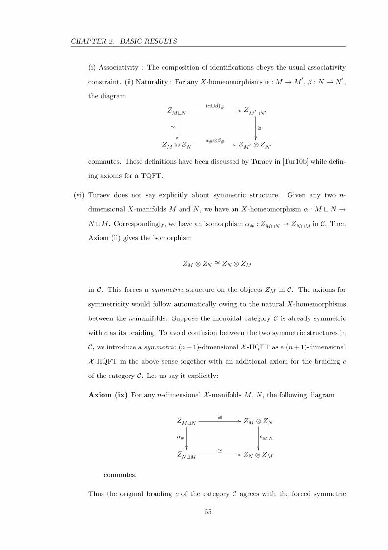
CHAPTER 2. BASIC RESULTS
(i) Associativity : The composition of identifications obeys the usual associativity
constraint. (ii) Naturality : For any X-homeomorphisms α : M →M′, β : N → N
′,
the diagram
ZMtN
∼=
��
(αtβ)# // ZM ′tN ′
∼=
��ZM ⊗ ZN
α#⊗β# // ZM ′ ⊗ ZN ′
commutes. These definitions have been discussed by Turaev in [Tur10b] while defin-
ing axioms for a TQFT.
(vi) Turaev does not say explicitly about symmetric structure. Given any two n-
dimensional X-manifolds M and N , we have an X-homeomorphism α : M tN →
N tM . Correspondingly, we have an isomorphism α# : ZMtN → ZNtM in C. Then
Axiom (ii) gives the isomorphism
ZM ⊗ ZN ∼= ZN ⊗ ZM
in C. This forces a symmetric structure on the objects ZM in C. The axioms for
symmetricity would follow automatically owing to the natural X-homemorphisms
between the n-manifolds. Suppose the monoidal category C is already symmetric
with c as its braiding. To avoid confusion between the two symmetric structures in
C, we introduce a symmetric (n+ 1)-dimensional X -HQFT as a (n+ 1)-dimensional
X -HQFT in the above sense together with an additional axiom for the braiding c
of the category C. Let us say it explicitly:
Axiom (ix) For any n-dimensional X -manifolds M , N , the following diagram
ZMtN
α#
��
∼= // ZM ⊗ ZN
cM,N
��ZNtM
∼= // ZN ⊗ ZM
commutes.
Thus the original braiding c of the category C agrees with the forced symmetric
55
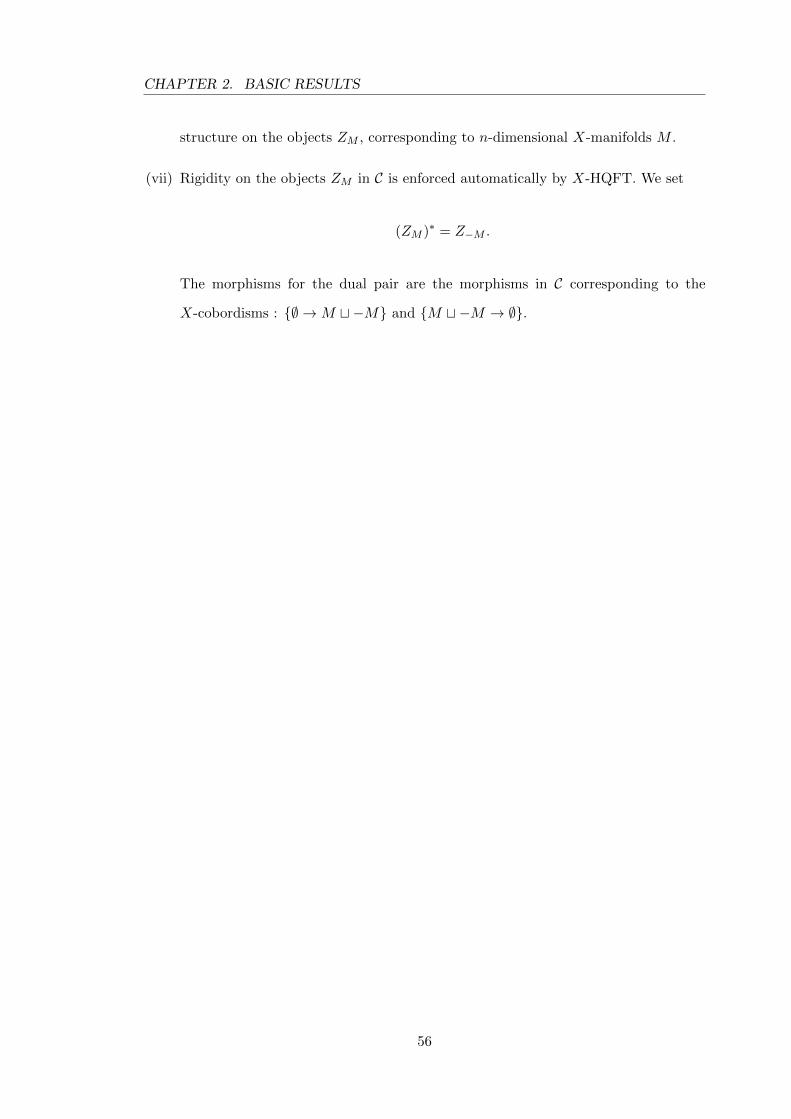
CHAPTER 2. BASIC RESULTS
structure on the objects ZM , corresponding to n-dimensional X-manifolds M .
(vii) Rigidity on the objects ZM in C is enforced automatically by X-HQFT. We set
(ZM )∗ = Z−M .
The morphisms for the dual pair are the morphisms in C corresponding to the
X-cobordisms : {∅ →M t −M} and {M t −M → ∅}.
56
Chapter 3
Crossed Systems
In this chapter we introduce the crossed algebras discovered by Turaev. We discuss
Homotopy Quantum Field Theory(HQFT) in dimension 2. Finally, we give examples of
crossed algebras in a category with twisted associativity. Throughout this chapter, let G
be a multiplicative group with a unit e, K a ground field.
3.1 G-coalgebras
A group-coalgebra [Vir02] (or simply a G-coalgebra when the group is known) is a
datum ({Cg}, {∆h,g}, ε) with h, g ∈ G satisfying the following axioms for all f, g, h ∈ G:
(1) Cg is a vector space,
(2) ∆f,g : Cfg → Cf ⊗ Cg, ε : Ce → K are linear maps,
(3) (id⊗∆g,h) ◦∆f,gh = (∆f,g ⊗ id) ◦∆fg,h : Cfgh → Cf ⊗ Cg ⊗ Ch,
(4) (id⊗ ε) ◦∆g,e = id : Ag → Ag,
(5) (ε⊗ id) ◦∆e,g = id : Ag → Ag.
Any G-graded coalgebra gives rise to a G-coalgebra by considering the graded com-
ponents of the coalgebra and its structure maps. The opposite is true only for finite
groups since if one defines C = ⊕Cg, the comultiplication ∆ = ⊕f,g∆f,g is not necessar-
ily well-defined. Essentially, group coalgebras are “local” versions of graded coalgebras.
The group coalgebras admit two important generalisations. First, one can talk about
G-coalgebras in any monoidal category. Second, one can talk about G-coalgebras for
non-discrete group or group schemes which we do in the next chapter.
57
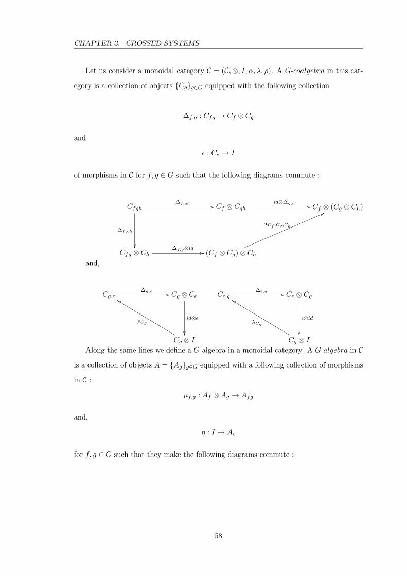
CHAPTER 3. CROSSED SYSTEMS
Let us consider a monoidal category C = (C,⊗, I, α, λ, ρ). A G-coalgebra in this cat-
egory is a collection of objects {Cg}g∈G equipped with the following collection
∆f,g : Cfg → Cf ⊗ Cg
and
ε : Ce → I
of morphisms in C for f, g ∈ G such that the following diagrams commute :
Cfgh∆f,gh //
∆fg,h
��
Cf ⊗ Cghid⊗∆g,h // Cf ⊗ (Cg ⊗ Ch)
Cfg ⊗ Ch∆f,g⊗id // (Cf ⊗ Cg)⊗ Ch
αCf ,Cg,Ch
66mmmmmmmmmmmmmmmmmmmmmmmmmm
and,
Cg.e∆g,e // Cg ⊗ Ce
id⊗ε
��Cg ⊗ I
ρCg
eeLLLLLLLLLLLLLLLLLLLL
Ce.g∆e,g // Ce ⊗ Cg
ε⊗id
��Cg ⊗ I
λCg
eeLLLLLLLLLLLLLLLLLLLL
Along the same lines we define a G-algebra in a monoidal category. A G-algebra in C
is a collection of objects A = {Ag}g∈G equipped with a following collection of morphisms
in C :
µf,g : Af ⊗Ag → Afg
and,
η : I → Ae
for f, g ∈ G such that they make the following diagrams commute :
58
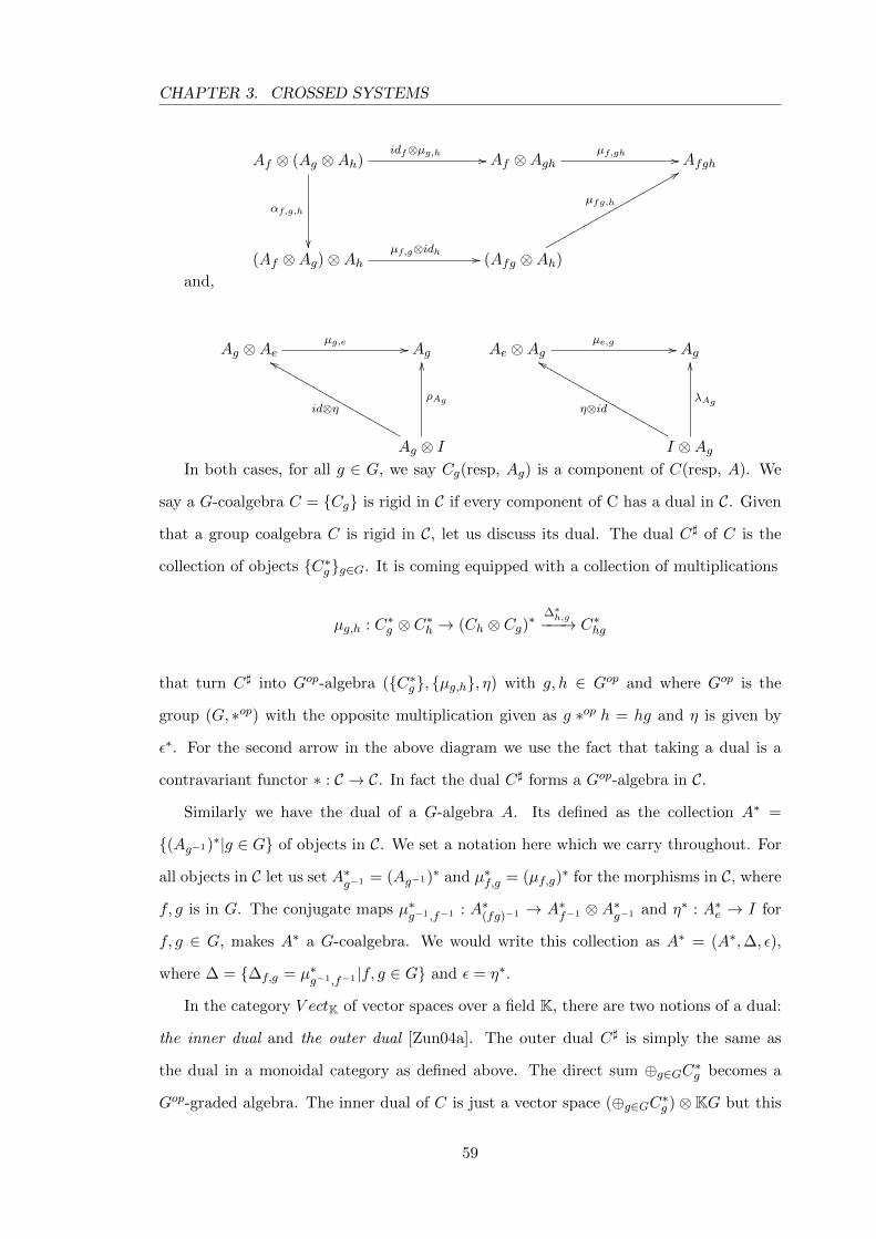
CHAPTER 3. CROSSED SYSTEMS
Af ⊗ (Ag ⊗Ah)idf⊗µg,h //
αf,g,h
��
Af ⊗Aghµf,gh // Afgh
(Af ⊗Ag)⊗Ahµf,g⊗idh // (Afg ⊗Ah)
µfg,h
88qqqqqqqqqqqqqqqqqqqqq
and,
Ag ⊗Aeµg,e // Ag
Ag ⊗ I
id⊗η
ffMMMMMMMMMMMMMMMMMMMMM
ρAg
OOAe ⊗Ag
µe,g // Ag
I ⊗Ag
η⊗id
ffMMMMMMMMMMMMMMMMMMMMM
λAg
OO
In both cases, for all g ∈ G, we say Cg(resp, Ag) is a component of C(resp, A). We
say a G-coalgebra C = {Cg} is rigid in C if every component of C has a dual in C. Given
that a group coalgebra C is rigid in C, let us discuss its dual. The dual C] of C is the
collection of objects {C∗g}g∈G. It is coming equipped with a collection of multiplications
µg,h : C∗g ⊗ C∗h → (Ch ⊗ Cg)∗∆∗h,g−−−→ C∗hg
that turn C] into Gop-algebra ({C∗g}, {µg,h}, η) with g, h ∈ Gop and where Gop is the
group (G, ∗op) with the opposite multiplication given as g ∗op h = hg and η is given by
ε∗. For the second arrow in the above diagram we use the fact that taking a dual is a
contravariant functor ∗ : C → C. In fact the dual C] forms a Gop-algebra in C.
Similarly we have the dual of a G-algebra A. Its defined as the collection A∗ =
{(Ag−1)∗|g ∈ G} of objects in C. We set a notation here which we carry throughout. For
all objects in C let us set A∗g−1 = (Ag−1)∗ and µ∗f,g = (µf,g)∗ for the morphisms in C, where
f, g is in G. The conjugate maps µ∗g−1,f−1 : A∗(fg)−1 → A∗f−1 ⊗ A∗g−1 and η∗ : A∗e → I for
f, g ∈ G, makes A∗ a G-coalgebra. We would write this collection as A∗ = (A∗,∆, ε),
where ∆ = {∆f,g = µ∗g−1,f−1 |f, g ∈ G} and ε = η∗.
In the category V ectK of vector spaces over a field K, there are two notions of a dual:
the inner dual and the outer dual [Zun04a]. The outer dual C] is simply the same as
the dual in a monoidal category as defined above. The direct sum ⊕g∈GC∗g becomes a
Gop-graded algebra. The inner dual of C is just a vector space (⊕g∈GC∗g )⊗KG but this
59
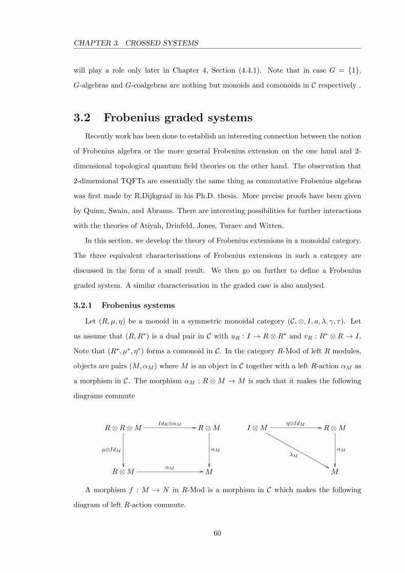
CHAPTER 3. CROSSED SYSTEMS
will play a role only later in Chapter 4, Section (4.4.1). Note that in case G = {1},
G-algebras and G-coalgebras are nothing but monoids and comonoids in C respectively .
3.2 Frobenius graded systems
Recently work has been done to establish an interesting connection between the notion
of Frobenius algebra or the more general Frobenius extension on the one hand and 2-
dimensional topological quantum field theories on the other hand. The observation that
2-dimensional TQFTs are essentially the same thing as commutative Frobenius algebras
was first made by R.Dijkgraaf in his Ph.D. thesis. More precise proofs have been given
by Quinn, Swain, and Abrams. There are interesting possibilities for further interactions
with the theories of Atiyah, Drinfeld, Jones, Turaev and Witten.
In this section, we develop the theory of Frobenius extensions in a monoidal category.
The three equivalent characterisations of Frobenius extensions in such a category are
discussed in the form of a small result. We then go on further to define a Frobenius
graded system. A similar characterisation in the graded case is also analysed.
3.2.1 Frobenius systems
Let (R,µ, η) be a monoid in a symmetric monoidal category (C,⊗, I, a, λ, γ, τ). Let
us assume that (R,R∗) is a dual pair in C with uR : I → R ⊗ R∗ and vR : R∗ ⊗ R → I.
Note that (R∗, µ∗, η∗) forms a comonoid in C. In the category R-Mod of left R modules,
objects are pairs (M,αM ) where M is an object in C together with a left R-action αM as
a morphism in C. The morphism αM : R ⊗M → M is such that it makes the following
diagrams commute
R⊗R⊗MIdR⊗αM //
µ⊗IdM
��
R⊗M
αM
��R⊗M
αM // M
I ⊗Mη⊗IdM //
λM
&&MMMMMMMMMMMMMMMMMMMMMM R⊗M
αM
��M
A morphism f : M → N in R-Mod is a morphism in C which makes the following
diagram of left R-action commute.
60
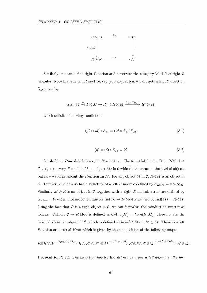
CHAPTER 3. CROSSED SYSTEMS
R⊗MαM //
IdR⊗f
��
M
f
��R⊗N
αN // N
Similarly one can define right R-action and construct the category Mod-R of right R
modules. Note that any left R module, say (M,αM ), automatically gets a left R∗-coaction
αM given by
αM : M∼=−→ I ⊗M −→ R∗ ⊗R⊗M idR∗⊗αM−−−−−−→ R∗ ⊗M,
which satisfies following conditions:
(µ∗ ⊗ id) ◦ αM = (id⊗ αM )αM , (3.1)
(η∗ ⊗ id) ◦ αM = id. (3.2)
Similarly an R-module has a right R∗-coaction. The forgetful functor For : R-Mod→
C assigns to every R-module M , an object MC in C which is the same on the level of objects
but now we forget about the R-action on M . For any object M in C, R⊗M is an object in
C. However, R⊗M also has a structure of a left R module defined by αR⊗M = µ⊗ IdM .
Similarly M ⊗ R is an object in C together with a right R module structure defined by
αN⊗R = IdN⊗µ. The induction functor Ind : C → R-Mod is defined by Ind(M) = R⊗M .
Using the fact that R is a rigid object in C, we can formalise the coinduction functor as
follows. CoInd : C → R-Mod is defined as CoInd(M) = hom(R,M). Here hom is the
internal Hom, an object in C, which is defined as hom(R,M) = R∗ ⊗M . There is a left
R-action on internal Hom which is given by the composition of the following maps:
R⊗R∗⊗M IdR⊗µ∗⊗IdM−−−−−−−−−→ R⊗R∗ ⊗R∗ ⊗M τ⊗IdR∗⊗M−−−−−−−→ R∗⊗R⊗R∗⊗MvR⊗Id∗R⊗IdM−−−−−−−−−→ R∗⊗M.
Proposition 3.2.1 The induction functor Ind defined as above is left adjoint to the for-
61
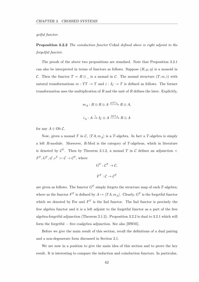
CHAPTER 3. CROSSED SYSTEMS
getful functor.
Proposition 3.2.2 The coinduction functor CoInd defined above is right adjoint to the
forgetful functor.
The proofs of the above two propositions are standard. Note that Proposition 3.2.1
can also be interpreted in terms of functors as follows. Suppose (R,µ, η) is a monoid in
C. Then the functor T = R ⊗ is a monad in C. The monad structure (T,m, i) with
natural transformations m : TT → T and i : IC → T is defined as follows. The former
transformation uses the multiplication of R and the unit of R defines the later. Explicitly,
mA : R⊗R⊗A µ⊗1A−−−→ R⊗A,
iA : Aγ−→ IC ⊗A
η⊗1A−−−→ R⊗A
for any A ∈ Ob C.
Now, given a monad T in C, 〈TA,mA〉 is a T -algebra. In fact a T -algebra is simply
a left R-module. Moreover, R-Mod is the category of T -algebras, which in literature
is denoted by CT . Then by Theorem 2.1.2, a monad T in C defines an adjunction <
F T , GT , ηt, εT >: C → CT , where
GT : CT → C,
F T : C → CT
are given as follows. The functor GT simply forgets the structure map of each T -algebra;
where as the functor F T is defined by A 7→ 〈TA,mA〉. Clearly, GT is the forgetful functor
which we denoted by For and F T is the Ind functor. The Ind functor is precisely the
free algebra functor and it is a left adjoint to the forgetful functor as a part of the free
algebra-forgetful adjunction (Theorem 2.1.2). Proposition 3.2.2 is dual to 3.2.1 which will
form the forgetful − free coalgebra adjunction. See also [BW05].
Before we give the main result of this section, recall the definitions of a dual pairing
and a non-degenerate form discussed in Section 2.1.
We are now in a position to give the main idea of this section and to prove the key
result. It is interesting to compare the induction and coinduction functors. In particular,
62
CHAPTER 3. CROSSED SYSTEMS
we want to see what happens if they are isomorphic.
Definition 3.2.3 We say the monoid (R,µ, η) is a Frobenius extension if the associated
induction and coinduction functors are naturally isomorphic.
In particular, in the category of R-modules the natural isomorphism essentially means
R⊗M ∼= M ⊗R∗ for any R-module M .
Remark. Propositions 3.2.1 and 3.2.2 implies respectively that the functors Ind and
CoInd are left and right adjoint to For. Then another way of looking at Definition 3.2.4
of a Frobenius extension is that Ind (or CoInd) is at the same time a left and a right
adjoint of the forgetful functor. Thus Definition 3.2.4 is equivalent to say that R⊗ is a
Frobenius functor.
Proposition 3.2.4 Let (R,µ, η) be a rigid monoid in a monoidal category C. Then the
folowing are equivalent :
(i) The dual object R∗ of R is a left R module and R is isomorphic to R∗ in R-Mod.
(ii) There exists a morphism ∆ : R → R ⊗ R in R-Mod and a morphism ε : R → I in
C, such that (Id⊗∆) ◦∆ = (∆⊗ Id) ◦∆ and (Id⊗ ε) ◦∆ = Id = (ε⊗ Id) ◦∆. And,
ε gives rise to a non-degenerate pairing :
R⊗R ε.µ−−→ I.
with :
I∆.η−−→ R⊗R.
as its copairing.
(iii) (R,µ, η) is a Frobenius extension.
Proof: (i) ⇐⇒ (ii). Given that φ : RR ∼= RR∗, define ∆ as the composition of the
following maps:
Rφ−→ R∗
µ∗−→ R∗ ⊗R∗ φ−1⊗φ−1
−−−−−−→ R⊗R.
The composition
Rφ−→ R∗
η∗−→ I
63
CHAPTER 3. CROSSED SYSTEMS
gives ε. Its easy to check that axioms are satisfied. The non-degeneracy of ε follows from
the axioms of dual of R. Conversely,
R⊗R µ−→ Rε−→ I
and,
Iη−→ R
∆−→ R⊗R
together with the non-degeneracy of ε implies that R ∼= R∗ in C.
(i) ⇐⇒ (iii). Given that φ : RR ∼= RR∗, then automatically, R ⊗M ∼= R∗ ⊗M
holds functorially. Conversely, substituting the unit object into the natural isomorphism
of functors gives the required isomorphism in R-Mod.
2
Remark. In this case we say (R,µ, η,∆, ε) forms a Frobenius system in C. Note here
that a Frobenius system is a Frobenius extension with a fixed natural isomorphism. In the
case when we are in the category of vector spaces over a ground field K, a monoid (R,µ, η)
is a K-algebra. A Frobenius extension is a Frobenius K-algebra whereas a Frobenius
system is a Frobenius K-algebra with a fixed pairing.
Examples. It is easy to show that first three examples below are Frobenius systems.
The first one was studied by Khovanov [Kho00]. The third one was studied by Lee
[Lee05]. In the first three examples, we are considering the category of I-modules, and
provide a Frobenius system F = (R,∆, ε) in these categories. The last example, discussed
by Brzezinski [Brz00], gives a Frobenius extension starting from an entwining structures
over a ground field K.
(i) I = Z and R = Z[X] / < X2 >
∆(1) = 1⊗X +X ⊗ 1 ε(1) = 0
∆(X) = X ⊗X ε(X) = 1.
(ii) I = Z[c] and R = Z[X, c] /< X2 >
∆(1) = 1⊗X +X ⊗ 1 + cZ ⊗X ε(1) = −c
64
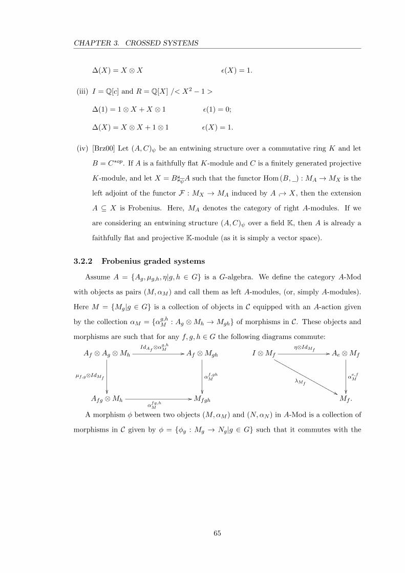
CHAPTER 3. CROSSED SYSTEMS
∆(X) = X ⊗X ε(X) = 1.
(iii) I = Q[c] and R = Q[X] /< X2 − 1 >
∆(1) = 1⊗X +X ⊗ 1 ε(1) = 0;
∆(X) = X ⊗X + 1⊗ 1 ε(X) = 1.
(iv) [Brz00] Let (A,C)ψ be an entwining structure over a commutative ring K and let
B = C∗op. If A is a faithfully flat K-module and C is a finitely generated projective
K-module, and let X = B]ψA such that the functor Hom(B, ) : MA →MX is the
left adjoint of the functor F : MX → MA induced by A ↪→ X, then the extension
A ⊆ X is Frobenius. Here, MA denotes the category of right A-modules. If we
are considering an entwining structure (A,C)ψ over a field K, then A is already a
faithfully flat and projective K-module (as it is simply a vector space).
3.2.2 Frobenius graded systems
Assume A = {Ag, µg,h, η|g, h ∈ G} is a G-algebra. We define the category A-Mod
with objects as pairs (M,αM ) and call them as left A-modules, (or, simply A-modules).
Here M = {Mg|g ∈ G} is a collection of objects in C equipped with an A-action given
by the collection αM = {αg,hM : Ag ⊗Mh → Mgh} of morphisms in C. These objects and
morphisms are such that for any f, g, h ∈ G the following diagrams commute:
Af ⊗Ag ⊗Mh
IdAf⊗αg,hM //
µf,g⊗IdMf
��
Af ⊗Mgh
αf,ghM
��Afg ⊗Mh
αfg,hM
// Mfgh
I ⊗Mf
η⊗IdMf //
λMf
&&MMMMMMMMMMMMMMMMMMMMMMAe ⊗Mf
αe,fM
��Mf .
A morphism φ between two objects (M,αM ) and (N,αN ) in A-Mod is a collection of
morphisms in C given by φ = {φg : Mg → Ng|g ∈ G} such that it commutes with the
65
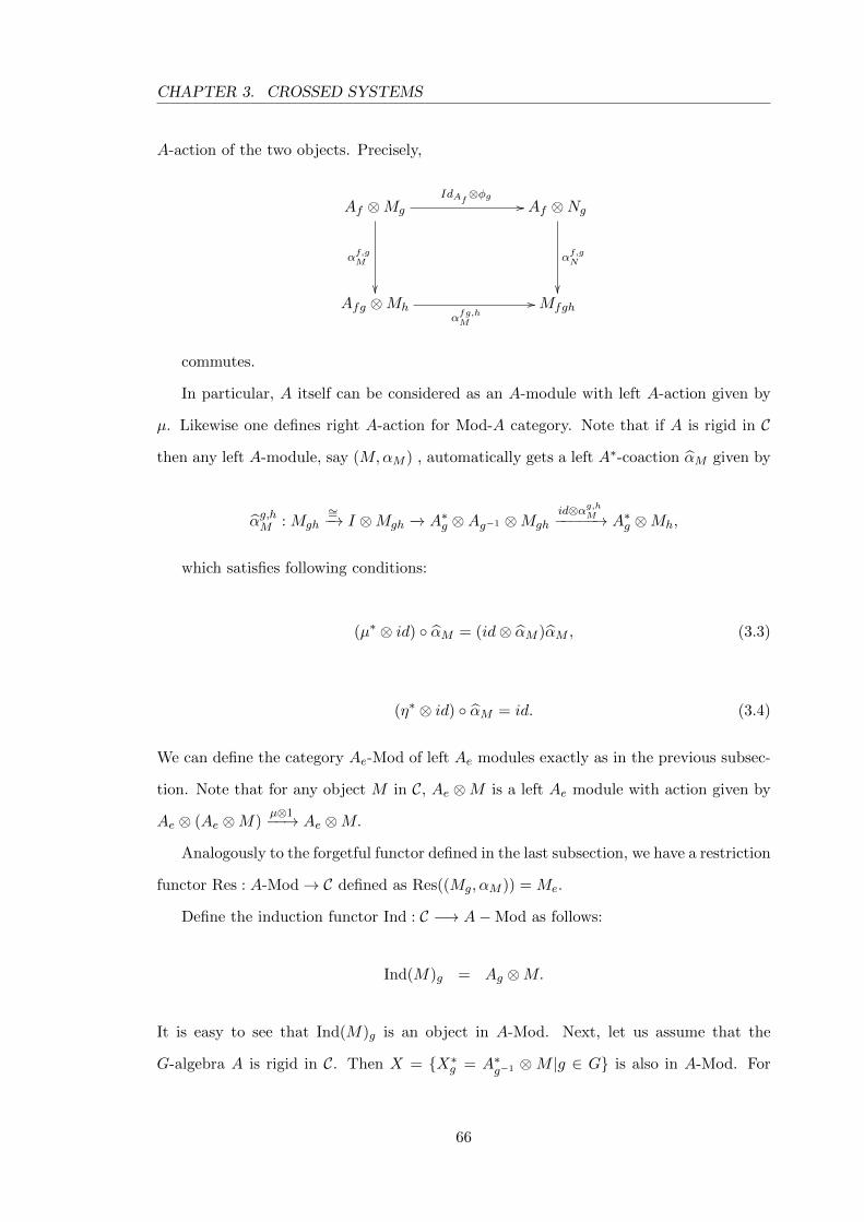
CHAPTER 3. CROSSED SYSTEMS
A-action of the two objects. Precisely,
Af ⊗Mg
IdAf⊗φg //
αf,gM
��
Af ⊗Ng
αf,gN
��Afg ⊗Mh
αfg,hM
// Mfgh
commutes.
In particular, A itself can be considered as an A-module with left A-action given by
µ. Likewise one defines right A-action for Mod-A category. Note that if A is rigid in C
then any left A-module, say (M,αM ) , automatically gets a left A∗-coaction αM given by
αg,hM : Mgh
∼=−→ I ⊗Mgh −→ A∗g ⊗Ag−1 ⊗Mghid⊗αg,hM−−−−−→ A∗g ⊗Mh,
which satisfies following conditions:
(µ∗ ⊗ id) ◦ αM = (id⊗ αM )αM , (3.3)
(η∗ ⊗ id) ◦ αM = id. (3.4)
We can define the category Ae-Mod of left Ae modules exactly as in the previous subsec-
tion. Note that for any object M in C, Ae ⊗M is a left Ae module with action given by
Ae ⊗ (Ae ⊗M)µ⊗1−−→ Ae ⊗M.
Analogously to the forgetful functor defined in the last subsection, we have a restriction
functor Res : A-Mod→ C defined as Res((Mg, αM )) = Me.
Define the induction functor Ind : C −→ A−Mod as follows:
Ind(M)g = Ag ⊗M.
It is easy to see that Ind(M)g is an object in A-Mod. Next, let us assume that the
G-algebra A is rigid in C. Then X = {X∗g = A∗g−1 ⊗M |g ∈ G} is also in A-Mod. For
66
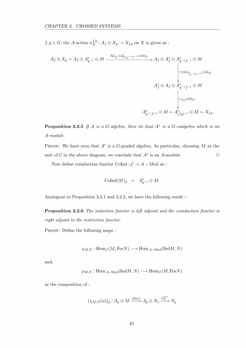
CHAPTER 3. CROSSED SYSTEMS
f, g ∈ G, the A-action αf,gX : Af ⊗Xg → Xfg on X is given as :
Af ⊗Xg = Af ⊗A∗g−1 ⊗MIdAf⊗∆f,g−1f−1⊗IdM
// Af ⊗A∗f ⊗A∗g−1f−1 ⊗M
τ⊗IdAg−1f−1
⊗IdM
��A∗f ⊗Af ⊗A∗g−1f−1 ⊗M
vAf⊗IdM
��A∗g−1f−1 ⊗M = A∗(fg)−1 ⊗M = Xfg.
Proposition 3.2.5 If A is a G-algebra, then its dual A∗ is a G-coalgebra which is an
A-module.
Proof: We have seen that A∗ is a G-graded algebra. In particular, choosing M as the
unit of C in the above diagram, we conclude that A∗ is an A-module. 2
Now define coinduction functor CoInd : C → A−Mod as :
CoInd(M)g = A∗g−1 ⊗M.
Analogous to Proposition 3.2.1 and 3.2.2, we have the following result :
Proposition 3.2.6 The induction functor is left adjoint and the coinduction functor is
right adjoint to the restriction functor.
Proof: Define the following maps :
χM,N : Hom C(M,ForN) −→ HomA−Mod(IndM,N)
and,
ρM,N : HomA−Mod(IndM,N) −→ Hom C(M,ForN)
as the composition of :
(χM,N (φ))g : Ag ⊗Mid⊗φ−−−→ Ag ⊗Ne
αg,eN−−→ Ng
67
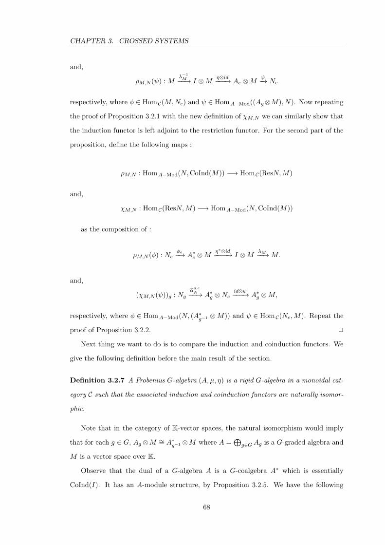
CHAPTER 3. CROSSED SYSTEMS
and,
ρM,N (ψ) : Mλ−1M−−→ I ⊗M η⊗id−−−→ Ae ⊗M
ψ−→ Ne
respectively, where φ ∈ Hom C(M,Ne) and ψ ∈ HomA−Mod((Ag⊗M), N). Now repeating
the proof of Proposition 3.2.1 with the new definition of χM,N we can similarly show that
the induction functor is left adjoint to the restriction functor. For the second part of the
proposition, define the following maps :
ρM,N : HomA−Mod(N,CoInd(M)) −→ Hom C(ResN,M)
and,
χM,N : Hom C(ResN,M) −→ HomA−Mod(N,CoInd(M))
as the composition of :
ρM,N (φ) : Neφe−→ A∗e ⊗M
η∗⊗id−−−−→ I ⊗M λM−−→M.
and,
(χM,N (ψ))g : Ngαg,eN−−→ A∗g ⊗Ne
id⊗ψ−−−→ A∗g ⊗M,
respectively, where φ ∈ HomA−Mod(N, (A∗g−1 ⊗M)) and ψ ∈ Hom C(Ne,M). Repeat the
proof of Proposition 3.2.2. 2
Next thing we want to do is to compare the induction and coinduction functors. We
give the following definition before the main result of the section.
Definition 3.2.7 A Frobenius G-algebra (A,µ, η) is a rigid G-algebra in a monoidal cat-
egory C such that the associated induction and coinduction functors are naturally isomor-
phic.
Note that in the category of K-vector spaces, the natural isomorphism would imply
that for each g ∈ G, Ag⊗M ∼= A∗g−1 ⊗M where A =⊕
g∈GAg is a G-graded algebra and
M is a vector space over K.
Observe that the dual of a G-algebra A is a G-coalgebra A∗ which is essentially
CoInd(I). It has an A-module structure, by Proposition 3.2.5. We have the following
68
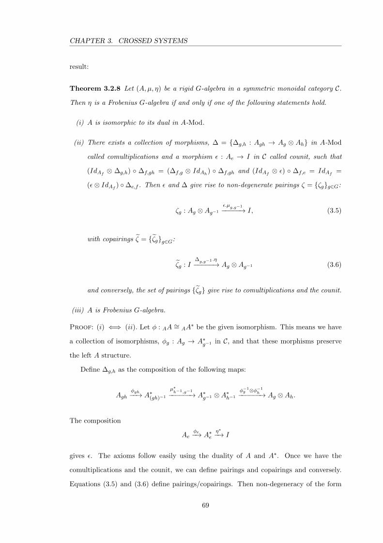
CHAPTER 3. CROSSED SYSTEMS
result:
Theorem 3.2.8 Let (A,µ, η) be a rigid G-algebra in a symmetric monoidal category C.
Then η is a Frobenius G-algebra if and only if one of the following statements hold.
(i) A is isomorphic to its dual in A-Mod.
(ii) There exists a collection of morphisms, ∆ = {∆g,h : Agh → Ag ⊗ Ah} in A-Mod
called comultiplications and a morphism ε : Ae → I in C called counit, such that
(IdAf ⊗ ∆g,h) ◦ ∆f,gh = (∆f,g ⊗ IdAh) ◦ ∆f,gh and (IdAf ⊗ ε) ◦ ∆f,e = IdAf =
(ε⊗ IdAf ) ◦∆e,f . Then ε and ∆ give rise to non-degenerate pairings ζ = {ζg}g∈G:
ζg : Ag ⊗Ag−1
ε.µg,g−1
−−−−−→ I, (3.5)
with copairings ζ = {ζg}g∈G:
ζg : I∆g,g−1 .η−−−−−→ Ag ⊗Ag−1 (3.6)
and conversely, the set of pairings {ζg} give rise to comultiplications and the counit.
(iii) A is Frobenius G-algebra.
Proof: (i) ⇐⇒ (ii). Let φ : AA ∼= AA∗ be the given isomorphism. This means we have
a collection of isomorphisms, φg : Ag → A∗g−1 in C, and that these morphisms preserve
the left A structure.
Define ∆g,h as the composition of the following maps:
Aghφgh−−→ A∗(gh)−1
µ∗h−1,g−1
−−−−−−→ A∗g−1 ⊗A∗h−1
φ−1g ⊗φ−1
h−−−−−−→ Ag ⊗Ah.
The composition
Aeφe−→ A∗e
η∗−→ I
gives ε. The axioms follow easily using the duality of A and A∗. Once we have the
comultiplications and the counit, we can define pairings and copairings and conversely.
Equations (3.5) and (3.6) define pairings/copairings. Then non-degeneracy of the form
69
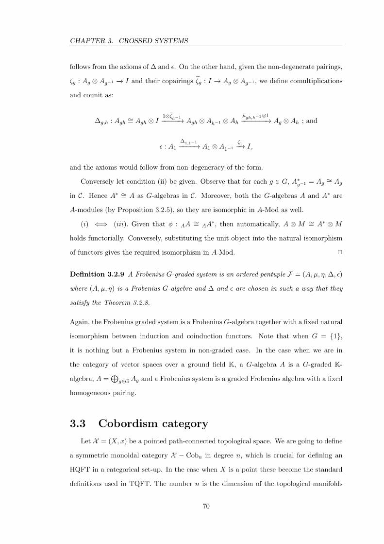
CHAPTER 3. CROSSED SYSTEMS
follows from the axioms of ∆ and ε. On the other hand, given the non-degenerate pairings,
ζg : Ag ⊗ Ag−1 −→ I and their copairings ζg : I → Ag ⊗ Ag−1 , we define comultiplications
and counit as:
∆g,h : Agh ∼= Agh ⊗ I1⊗ζh−1−−−−−→ Agh ⊗Ah−1 ⊗Ah
µgh,h−1⊗1−−−−−−−→ Ag ⊗Ah ; and
ε : A1
∆1,1−1
−−−−→ A1 ⊗A1−1
ζ1−→ I,
and the axioms would follow from non-degeneracy of the form.
Conversely let condition (ii) be given. Observe that for each g ∈ G, A∗g−1 = Ag ∼= Ag
in C. Hence A∗ ∼= A as G-algebras in C. Moreover, both the G-algebras A and A∗ are
A-modules (by Proposition 3.2.5), so they are isomorphic in A-Mod as well.
(i) ⇐⇒ (iii). Given that φ : AA ∼= AA∗, then automatically, A ⊗M ∼= A∗ ⊗M
holds functorially. Conversely, substituting the unit object into the natural isomorphism
of functors gives the required isomorphism in A-Mod. 2
Definition 3.2.9 A Frobenius G-graded system is an ordered pentuple F = (A,µ, η,∆, ε)
where (A,µ, η) is a Frobenius G-algebra and ∆ and ε are chosen in such a way that they
satisfy the Theorem 3.2.8.
Again, the Frobenius graded system is a Frobenius G-algebra together with a fixed natural
isomorphism between induction and coinduction functors. Note that when G = {1},
it is nothing but a Frobenius system in non-graded case. In the case when we are in
the category of vector spaces over a ground field K, a G-algebra A is a G-graded K-
algebra, A =⊕
g∈GAg and a Frobenius system is a graded Frobenius algebra with a fixed
homogeneous pairing.
3.3 Cobordism category
Let X = (X,x) be a pointed path-connected topological space. We are going to define
a symmetric monoidal category X − Cobn in degree n, which is crucial for defining an
HQFT in a categorical set-up. In the case when X is a point these become the standard
definitions used in TQFT. The number n is the dimension of the topological manifolds
70
CHAPTER 3. CROSSED SYSTEMS
considered as objects.
We start by defining a weak 2-category X − Cobn. It is weak in two senses. First,
the associativity and the identity properties of compositions of 1-morphisms holds only
up to a 2-isomorphism. Second, the composition of 2-morphisms is not associative either,
although one could make it associative up to a 3-morphism by turning X − Cobn into a
3-category. The weak 2-category X − Cobn plays an auxiliary role and its exact axioms
are of no significance for the further discussion.
We want to avoid set-theoretical differences, so we draw our manifolds from a suffi-
ciently large universum. By a manifold we understand a compact oriented topological
manifold with boundary. A closed manifold would mean a manifold in the above sense
but now without boundary. Sufficiently large means that each manifold will have a home-
omorphic manifold in the universum. The dimension of a manifold is the dimension of
any of its components that must be equal for the dimension to exist.
Let us start by describing objects (0-morphisms) of X − Cobn. An object is a triple
M = (M,fM , pM ) where M , called the base space ofM, is a closed manifold of dimension
n, such that every component of M is a pointed closed oriented manifold, fM : M → X
is a continuous function and pM is a point on each component of M . It is convenient to
think of p as a function pM : π0(M) → M such that pM (X) ∈ X for any component X.
The continuous function fM , called as the characteristic map of M , is required to be a
morphism of pointed manifolds, that is, fM (pM (X)) = x for any X ∈ π0(M). That is to
say it sends the base points of all the components of M into x. We sometimes may also
refer M as an X -manifold. We think of the empty set as an n-dimensional manifold for
any n. There are unique functions f : ∅ → X and p : ∅ → ∅ that turn the empty set into
an object which we also denote ∅.
An X -homeomorphism of 0-morphisms Ψ : M → K is an orientation preserving
homeomorphism from M to K, sending base points of M onto those of K such that
fM = fKΨ where fM , fK are the characteristic maps of M, K respectively.
Before we describe 1-morphisms let us point out a couple of operations. We define the
disjoint union of 0-morphisms by (L, fL, pL)t (M,fM , pM ) = (LtM,fL t fM , pL t pM ).
Note that if M,N are pointed topological manifolds, then M tN is again a pointed topo-
71
CHAPTER 3. CROSSED SYSTEMS
logical manifold. Moreover, if they are oriented, then we can define a unique orientation
on the disjoint union. The orientation on M t N is such that the inclusion maps are
orientation-preserving. The map fL t fM : L tM → X is defined in the obvious way, as
discussed in Section (2.7). It is a continuous map and let us denote it by fLtM . Just as for
fL, we define pLtM = pLtpM : π0(LtM)→ LtM . Note that π0(LtM) = π0Ltπ0M .
Indeed, LtM = (L tM,fLtM , pLtM ) is an X -manifold and hence again a 0-morphism.
With the operation of disjoint union we wish to make X−Cobn into a symmetric monoidal
category. For shorthand we would simply write L tM. Further, for any manifold M ,
let −M be the same manifold with the opposite orientation. For M = (M,f, p), define
M∗ = (−M,f, p). Clearly, M∗ is again a 0-morphism.
Now 1-morphisms in X − Cobn are cobordisms over X . More precisely, a morphism
from M = (M,fM , pM ) to K = (K, fK , pK) is a triple A = (A, fA, αA) where A, called
the base space of A, is a manifold of dimension n + 1, fA : A → X is a continuous map,
called characteristic map of A, and αA : ∂A→ (−M)tK, called the boundary map of A,
is an X -homeomorphism. By 0-morphism related to A, we understand the 0-morphisms
M and K. A also has a canonical map pA : π0 : (δA)→ A referred to as pointed structure
on the boundary of A. We call ∂A0 = α−1A (−M) as the in-boundary and ∂A1 = α−1
A (K)
as out-boundary for A. So, the boundary map is αA = α0A tα1
A : ∂A0 t ∂A1 → −M tK.
The composition B ◦ A of two morphisms A : K → L and B : L → M is gluing over
the common boundary L. The manifold of the composition is A t B/ ∼ where the only
nontrivial equivalences a ∼ b occur when a ∈ ∂A, b ∈ ∂B and αA(a) = αB(b) ∈ L. There
is an advantage of working in the topological category here as the manifold structure
is uniquely defined on the gluing. Since L induces opposite orientation from A and B
respectively, thus the orientations of A and B are extended/continued on their gluing
B ◦A, see Section (2.8), Theorem (2.8.4). The characteristic map of AtB is fA t fB/ ∼.
Assume ∂(AtB/ ∼) = X tY , where X = α−1A (−K) ⊆ ∂A and Y = α−1
B (M) ⊆ ∂B, then
the boundary identification on the gluing is given by α{AtB/∼} = αA|X t αB|Y .
Notice that (C◦B)◦A is not equal to C◦(B◦A) but there is a canonical homeomorphism
between the underlying cobordisms preserving the additional data. We will come back to
it when we discuss the 2-morphisms.
72
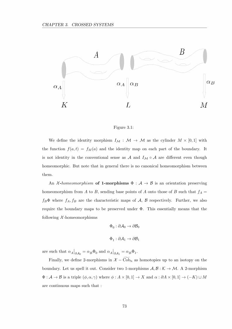
CHAPTER 3. CROSSED SYSTEMS
Figure 3.1:
We define the identity morphism IM : M → M as the cylinder M × [0, 1] with
the function f(a, t) = fM (a) and the identity map on each part of the boundary. It
is not identity in the conventional sense as A and IM ◦ A are different even though
homeomorphic. But note that in general there is no canonical homeomorphism between
them.
An X -homeomorphism of 1-morphisms Φ : A → B is an orientation preserving
homeomorphism from A to B, sending base points of A onto those of B such that fA =
fBΦ where fA, fB are the characteristic maps of A, B respectively. Further, we also
require the boundary maps to be preserved under Φ. This essentially means that the
following X -homeomorphisms
Φ0 : ∂A0 → ∂B0
Φ1 : ∂A1 → ∂B1
are such that αA∣∣∂A0
= αBΦ0 and αA∣∣∂A1
= αBΦ1.
Finally, we define 2-morphisms in X − Cobn as homotopies up to an isotopy on the
boundary. Let us spell it out. Consider two 1-morphisms A,B : K →M. A 2-morphism
Φ : A → B is a triple (φ, α, γ) where φ : A× [0, 1]→ X and α : ∂A× [0, 1]→ (−K) tM
are continuous maps such that :
73
CHAPTER 3. CROSSED SYSTEMS
(i) (A, φ0, α0) = A,
(ii) (A, φt, αt) is a 1-morphism from K to M for each t ∈ [0, 1].
(iii) γ : (A, φ1, α1)→ B is an X -homeomorphism of 1-morphisms.
The composition of 2-morphisms is defined by cutting the interval [0, 1] in half. This
composition is associative only up to homotopy (on [0, 1]). This is where 3-morphisms
appear! Similarly the trivial homotopy is identity 2-morphism only up to homotopy
and each 2-morphism admits an inverse up to homotopy. One can fix this by choosing
homotopy classes of 2-morphisms but we do not do it because our interest in 2-morphisms
is temporary.
We say that two 1-morphisms A,B : K → M are equivalent if there exists a 2-
morphism from A to B and in that case we write A ∼ B. We say 0-morphisms M =
(M,fM , pM ) andK = (K, fK , pK) are isomorphic if there are 1-morphismsA = (A, fA, αA)
and B = (B, fB, αB) from M to K and K to M respectively, such that IK ∼ A ◦ B and
IM ∼ B ◦ A. In this case we say B is an inverse of A.
Using an X -homeomorphisms Ψ between M = (M,fM , pM ) and K = (K, fK , pK) we
construct a 1-morphism AΨ = (M×I, fA, αΨA) fromM to K where fA is the projection of
the characteristic map of M and the boundary map αΨA is simply identity on in-boundary
and Ψ on out-boundary. We will generalise this concept and call them cylinders in the
next subsection.
Proposition 3.3.1 If Ψ and Φ are isotopic X -homeomorphisms betweenM = (M,fM , pM )
and K = (K, fK , pK) then the 1-morphisms AΨ and AΦ are equivalent in X − Cobn.
Proof: Since Ψ, Φ : M → K are isotopic, there exists a continuous path say H in the
space of X -homeomorphisms from M and K connecting Ψ and Φ. Now for AΨ and AΦ
to be equivalent we need to establish a 2-morphism (φ, α, γ) between them. If the space
of these 1-morphisms is A = M × I, the space of the two morphism is A× I. As M × I is
the space for the two 1-morphisms , result is trivial i.e. the A× I and the isotopy on the
out-boundary. Let us spell it out. The projection of the characteristic map of M gives
74
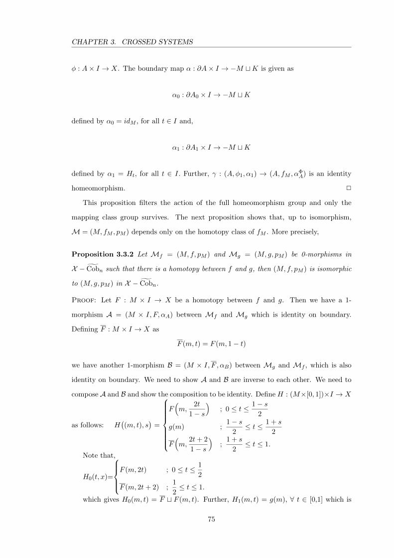
CHAPTER 3. CROSSED SYSTEMS
φ : A× I → X. The boundary map α : ∂A× I → −M tK is given as
α0 : ∂A0 × I → −M tK
defined by α0 = idM , for all t ∈ I and,
α1 : ∂A1 × I → −M tK
defined by α1 = Ht, for all t ∈ I. Further, γ : (A, φ1, α1) → (A, fM , αΦA) is an identity
homeomorphism. 2
This proposition filters the action of the full homeomorphism group and only the
mapping class group survives. The next proposition shows that, up to isomorphism,
M = (M,fM , pM ) depends only on the homotopy class of fM . More precisely,
Proposition 3.3.2 Let Mf = (M,f, pM ) and Mg = (M, g, pM ) be 0-morphisms in
X − Cobn such that there is a homotopy between f and g, then (M,f, pM ) is isomorphic
to (M, g, pM ) in X − Cobn.
Proof: Let F : M × I → X be a homotopy between f and g. Then we have a 1-
morphism A = (M × I, F, αA) between Mf and Mg which is identity on boundary.
Defining F : M × I → X as
F (m, t) = F (m, 1− t)
we have another 1-morphism B = (M × I, F , αB) between Mg and Mf , which is also
identity on boundary. We need to show A and B are inverse to each other. We need to
composeA and B and show the composition to be identity. Define H : (M×[0, 1])×I → X
as follows: H((m, t), s
)=
F(m,
2t
1− s
); 0 ≤ t ≤ 1− s
2
g(m) ;1− s
2≤ t ≤ 1 + s
2
F(m,
2t+ 2
1− s
);
1 + s
2≤ t ≤ 1.
Note that,
H0(t, x)=
F (m, 2t) ; 0 ≤ t ≤ 1
2
F (m, 2t+ 2) ;1
2≤ t ≤ 1.
which gives H0(m, t) = F t F (m, t). Further, H1(m, t) = g(m), ∀ t ∈ [0,1] which is
75
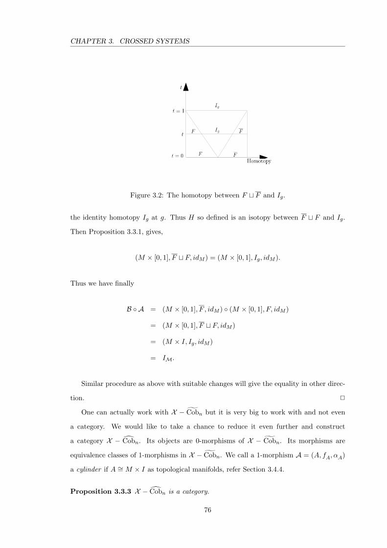
CHAPTER 3. CROSSED SYSTEMS
Figure 3.2: The homotopy between F t F and Ig.
the identity homotopy Ig at g. Thus H so defined is an isotopy between F t F and Ig.
Then Proposition 3.3.1, gives,
(M × [0, 1], F t F, idM ) = (M × [0, 1], Ig, idM ).
Thus we have finally
B ◦ A = (M × [0, 1], F , idM ) ◦ (M × [0, 1], F, idM )
= (M × [0, 1], F t F, idM )
= (M × I, Ig, idM )
= IM.
Similar procedure as above with suitable changes will give the equality in other direc-
tion. 2
One can actually work with X − Cobn but it is very big to work with and not even
a category. We would like to take a chance to reduce it even further and construct
a category X − Cobn. Its objects are 0-morphisms of X − Cobn. Its morphisms are
equivalence classes of 1-morphisms in X − Cobn. We call a 1-morphism A = (A, fA, αA)
a cylinder if A ∼= M × I as topological manifolds, refer Section 3.4.4.
Proposition 3.3.3 X − Cobn is a category.
76
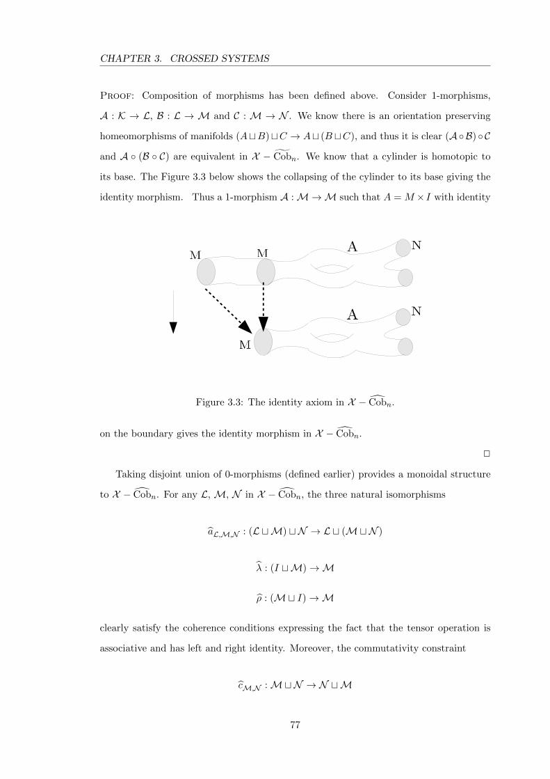
CHAPTER 3. CROSSED SYSTEMS
Proof: Composition of morphisms has been defined above. Consider 1-morphisms,
A : K → L, B : L → M and C : M → N . We know there is an orientation preserving
homeomorphisms of manifolds (AtB)tC → At (B tC), and thus it is clear (A◦B) ◦ C
and A ◦ (B ◦ C) are equivalent in X − Cobn. We know that a cylinder is homotopic to
its base. The Figure 3.3 below shows the collapsing of the cylinder to its base giving the
identity morphism. Thus a 1-morphism A :M→M such that A = M × I with identity
Figure 3.3: The identity axiom in X − Cobn.
on the boundary gives the identity morphism in X − Cobn.
2
Taking disjoint union of 0-morphisms (defined earlier) provides a monoidal structure
to X − Cobn. For any L, M, N in X − Cobn, the three natural isomorphisms
aL,M,N : (L tM) tN → L t (MtN )
λ : (I tM)→M
ρ : (Mt I)→M
clearly satisfy the coherence conditions expressing the fact that the tensor operation is
associative and has left and right identity. Moreover, the commutativity constraint
cM,N :MtN → N tM
77
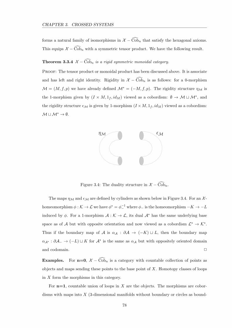
CHAPTER 3. CROSSED SYSTEMS
forms a natural family of isomorphisms in X − Cobn that satisfy the hexagonal axioms.
This equips X − Cobn with a symmetric tensor product. We have the following result.
Theorem 3.3.4 X − Cobn is a rigid symmetric monoidal category.
Proof: The tensor product or monoidal product has been discussed above. It is associate
and has left and right identity. Rigidity in X − Cobn is as follows: for a 0-morphism
M = (M,f, p) we have already defined M∗ = (−M,f, p). The rigidity structure ηM is
the 1-morphism given by (I ×M, 1f , idM ) viewed as a cobordism: ∅ → M tM∗, and
the rigidity structure εM is given by 1-morphism (I×M, 1f , idM ) viewed as a cobordism:
MtM∗ → ∅.
Figure 3.4: The duality structure in X − Cobn.
The maps ηM and εM are defined by cylinders as shown below in Figure 3.4. For an X -
homeomorphism φ : K → L we have φ∗ = φ−1− where φ− is the homeomorphism−K → −L
induced by φ. For a 1-morphism A : K → L, its dual A∗ has the same underlying base
space as of A but with opposite orientation and now viewed as a cobordism L∗ → K∗.
Thus if the boundary map of A is αA : ∂A → (−K) t L, then the boundary map
αA∗ : ∂A− → (−L) tK for A∗ is the same as αA but with oppositely oriented domain
and codomain. 2
Examples. For n=0, X − Cobn is a category with countable collection of points as
objects and maps sending these points to the base point of X. Homotopy classes of loops
in X form the morphisms in this category.
For n=1, countable union of loops in X are the objects. The morphisms are cobor-
disms with maps into X (3-dimensional manifolds without boundary or circles as bound-
78
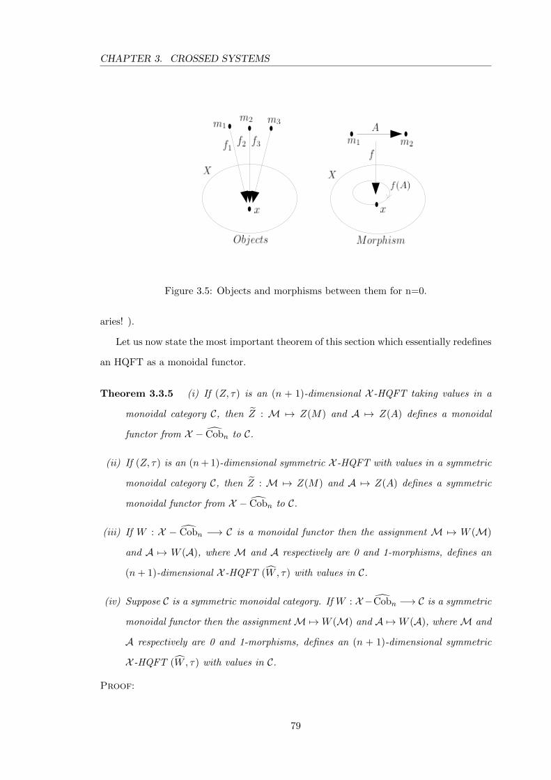
CHAPTER 3. CROSSED SYSTEMS
Figure 3.5: Objects and morphisms between them for n=0.
aries! ).
Let us now state the most important theorem of this section which essentially redefines
an HQFT as a monoidal functor.
Theorem 3.3.5 (i) If (Z, τ) is an (n + 1)-dimensional X -HQFT taking values in a
monoidal category C, then Z : M 7→ Z(M) and A 7→ Z(A) defines a monoidal
functor from X − Cobn to C.
(ii) If (Z, τ) is an (n+ 1)-dimensional symmetric X -HQFT with values in a symmetric
monoidal category C, then Z : M 7→ Z(M) and A 7→ Z(A) defines a symmetric
monoidal functor from X − Cobn to C.
(iii) If W : X − Cobn −→ C is a monoidal functor then the assignment M 7→ W (M)
and A 7→ W (A), where M and A respectively are 0 and 1-morphisms, defines an
(n+ 1)-dimensional X -HQFT (W , τ) with values in C.
(iv) Suppose C is a symmetric monoidal category. If W : X −Cobn −→ C is a symmetric
monoidal functor then the assignmentM 7→W (M) and A 7→W (A), whereM and
A respectively are 0 and 1-morphisms, defines an (n + 1)-dimensional symmetric
X -HQFT (W , τ) with values in C.
Proof:
79
CHAPTER 3. CROSSED SYSTEMS
(i) Let (Z, τ) be an (n+ 1)-dimensional X -HQFT taking values in a monoidal category
C. Let us define a functor Z : X − Cobn → C as Z : M 7→ Z(M) and Z :
A 7→ Z(A). The Axioms (ii) and (iii) of an HQFT gives the coherence morphisms
φM,N : Z(M)⊗ Z(N )→ Z(M⊗N ) and Z(∅)→ IC . The axioms for the coherence
maps would follow automatically owing to the natural X -homemorphisms between
the n-manifolds.
(ii) We have already shown in part (i) that Z is a monoidal functor. Axiom (ix) of a
symmetric HQFT makes Z a braided monoidal functor. Since X −Cobn and C are
symmetric monoidal categories, Z is a symmetric monoidal functor.
(iii) Consider a monoidal functor W : X − Cobn → C. We want to define an (n + 1)-
dimensional X -HQFT (W , τ) with values in C. Let us define it explicitly:
W (M) = W (M); M is a 0-morphism,
τ(A) : W (M)W (A)−−−−→W (N ); A :M→N is a 1-morphism.
Given an X -homeomorphism f : M → N we have a 1-morphism AM = (M ×
I, fA, αA), with fA = fm × 1, α0A = idM and α1
A = f : M → N . The inverse of
AM is again a 1-morphism given by BM = (M × I, fB, αB) with fB = fm × 1,
α0B = f : M → N and α1
B = idM . Then BM ◦AM = idM and similarly we have the
identity on N . Thus, the morphism in C corresponding to AM is an isomorphism.
So, we set
f# = W (AM) : W (M)W (AM)−−−−−→ W (N ); f :M→N is an X -homeomorphism.
We now discuss the axioms of an X -HQFT. For any X -homeomorphisms f : L →M
and f′
: M → N , (f′f)# = f
′#f# since W is a functor. Further, W being a
monoidal functor, we have W (MtN ) ∼= W (M)⊗ W (N ) and W (∅) ∼= IC . Axiom
(iv) follows from the way we have set up the category X − Cobn with morphisms as
equivalence classes of 1-morphisms up to 2-morphisms in X − Cobn. Axiom (v) is
obvious. As discussed before, we can consider any X -homeomorphism f :M→ N
80
CHAPTER 3. CROSSED SYSTEMS
as a 1-morphism (M × I, fM , α), where α0 = idM and α1 = f : M → N . Then
the gluing axiom becomes the composition of morphisms which is preserved by a
functor. The identity morphism AM for any 0-morphism M gives the Axiom (vii).
Finally the last axiom is a part of the definition of the category X − Cobn.
(iv) (W , τ) is an X -HQFT by part (iii). Axiom (ix) of an HQFT follows from the fact
that W is a symmetric monoidal functor.
2
So far we have worked with a single space X fixed in the background. Suppose
now we have two spaces X , Y which interact with each other via a continuous map.
Let us explore the interaction between the corresponding symmetric monoidal categories
X − Cobn and Y − Cobn; and the X -HQFTs and Y-HQFTs that one can construct
from X and Y. Suppose Ψ : X → Y is a continuous map of pointed path-connected
topological spaces, X = (X,x) and Y = (Y, y). If M = (M,fM , pM ) is a 0-morphism
in X − Cobn, then MY = (M,fYM = ΨfM , pM ) will be a 0-morphism in Y − Cobn.
In the same way, if A = (A, fA, αA) : M → K is a 1-morphism in X − Cobn then
AY = (A, fYA = ΨfA, αA) : (M,fYM , pM ) → (K, fYK , pK) is a 1-morphism in Y − Cobn.
These assignments induces a functor
Ψ∗ : X − Cobn → Y − Cobn
such that M 7→MY and A 7→ AY . Note that
MY tNY =(MtN , fYM t f
YN , pM t pN
)=
(MtN ,ΨfM tΨfN , pM t pN
)=
(MtN ,Ψ(fM t fN ), pM t pN
)=
(MtN ,Ψ(fMtN ), pM t pN
)=
(MtN , fYMtN , pM t pN
)= (MtN )Y .
81
CHAPTER 3. CROSSED SYSTEMS
Similarly,(
(LtM)tN)Y
= (LY tMY)tNY . This makes Ψ∗ a strict monoidal functor.
Further, observe that the following commutative diagram
MY tNY=
��
// NY tMY=
��(MtN )Y // (N tM)Y
relates the braidings in the two categories. Indeed the functor is symmetric in nature
(hexagonal axioms are obvious). Thus Ψ∗ is a strict symmetric monoidal functor.
Now let Ψ and Φ be continuous maps X → Y and H a homotopy between them.
If (M,fM , pM ) is a 0-morphism over X , then (M,ΨfM , pM ) and (M,ΦfM , pM ) are 0-
morphisms over Y. On the other hand, the map H ◦ (fM × I[0,1]) : M × [0, 1]→ Y defined
by
(m, t) 7→ H(fM (m), t)
is a homotopy between ΨfM and ΦfM , and by proposition (3.3.1), there is an isomorphism
between (M,ΨfM , pM ) and (M,ΦfM , pM ). This induces a natural isomorphism
η : Ψ∗ → Φ∗.
Definition 3.3.6 Given n ≥ 0, an n-homotopy equivalence between topological spaces is
a continuous map which induces isomorphisms on homotopy groups πk(X,x), k ≤ n.
The existence of an n-homotopy equivalence from X to Y is a reflexive and transitive
relation, but not symmetric. Thus we state that X and Y are weakly n-homotopy equiv-
alent if there exists a zigzag of n-homotopy equivalences X ← → ← · · · → Y . Homotopy
n-types are the equivalence classes of a weak n-homotopy equivalence relation. Thus, if
two spaces have the same homotopy n-type then their homotopy groups agree up to n.
Let us consider the category Zn+1(X , C) of (n + 1)-dimensional X -HQFTs taking
values in a monoidal category C. The objects are (n + 1)-dimensional X -HQFTs with
values in C. A morphism (Z, τ) → (Z′, τ′) in this category is a family of morphisms
{ρM : ZM → Z′M} where M runs over 0-morphisms in X − Cobn such that ρ∅ = IC
; for disjoint 0-morphisms M and N , we have ρMtN = ρM ⊗ ρN ; the natural square
82
CHAPTER 3. CROSSED SYSTEMS
diagrams associated with X -homeomorphisms of 0-morphisms and with 1-morphisms are
commutative. Note that if the monoidal category C in the background is clear and there
is no ambiguity, then we may simply use Zn+1(X ).
Observe that HQFTs can also be pushed forward along the maps between the target
spaces. Given a map Ψ : X → Y of path-connected pointed spaces we can transform
any X -HQFT into a Y-HQFT both taking values in the same domain monoidal category
C. It suffices to compose the characteristic maps with Ψ. This induces a functor Ψ∗ :
Zn+1(X , C)→ Zn+1(Y, C). We finally state the main result of the section. Note that the
credit of this theorem goes to Turaev who has established a similar theorem for any (n+1)-
type path connected topological spaces giving equivalence of the category of HQFTs over
them. For the proof see Theorem 2.2.1, [Tur99].
Theorem 3.3.7 Let n ≥ 0. If two path-connected pointed spaces X and Y have the same
homotopy (n+ 1)-type, then there exists a zigzag of functors Zn+1(X , C)← → ← · · · →
Zn+1(Y, C) which are equivalences of categories; thus
Zn+1(X , C) ∼ Zn+1(Y, C)
are equivalent categories.
Proof: Since X and Y have the same homotopy (n + 1)-type, they are connected by a
zigzag of n-homotopy equivalences X ← → ← · · · → Y which induces isomorphisms on
all homotopy groups up to n+ 1. 2
3.4 Crossed Systems
Inspired by the work done by Turaev on HQFTs [Tur99], we define Turaev G-crossed
system for a group G. We then define cylinders in an appropriate category and finally
we give one of the main results of this chapter that circles and cylinders form a Turaev
Crossed system. Let us first define this appropriate category (will call it X − Cobn) as
follows.
83
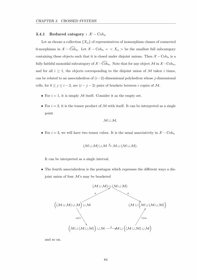
CHAPTER 3. CROSSED SYSTEMS
3.4.1 Reduced category : X − Cobn
Let us choose a collection {Xα} of representatives of isomorphism classes of connected
0-morphisms in X − Cobn. Let X − Cobn = < Xα > be the smallest full subcategory
containing these objects such that it is closed under disjoint unions. Then X −Cobn is a
fully faithful monoidal subcategory of X−Cobn. Note that for any objectM in X−Cobn,
and for all i ≥ 1, the objects corresponding to the disjoint union of M taken i times,
can be related to an associahedron of (i−2)-dimensional polyhedron whose j-dimensional
cells, for 0 ≤ j ≤ i− 2, are (i− j − 2) pairs of brackets between i copies of M.
• For i = 1, it is simply M itself. Consider it as the empty set.
• For i = 2, it is the tensor product ofM with itself. It can be interpreted as a single
point
MtM.
• For i = 3, we will have two tensor cubes. It is the usual associativity in X − Cobn
(MtM) tM a−→Mt (MtM).
It can be interpreted as a single interval.
• The fourth associahedron is the pentagon which expresses the different ways a dis-
joint union of four M’s may be bracketed
(MtM) t (MtM)
(Mt(Mt (MtM)
)
Mt(
(MtM) tM)(
Mt (MtM))tM
((MtM) tM
)tM
a
''OOOOOOOOOOOOOOOOOOO
1⊗a
EE������������a //
a⊗1
��222222222222
a
77ooooooooooooooooooo
and so on.
84
CHAPTER 3. CROSSED SYSTEMS
Thus we have an inclusion functor
G : X − Cobn ↪→ X − Cobn
which is such that each object X of X − Cobn is isomorphic to an object of X −Cobn. We
wish to formulate the inverse of this functor so that the inclusion functor G becomes an
equivalence of categories and X −Cobn becomes equivalent to X − Cobn. Let us explain
how to construct the inverse functor and hence the equivalence.
Theorem 3.4.1 The functor G : X − Cobn ↪→ X − Cobn is a symmetric monoidal
equivalence.
Proof: For each object X in X − Cobn, let us choose an object FX and an isomorphism
θX : X → FX of X −Cobn which sends x 7→ Fx and its inverse sends y 7→ y. Suppose A
is a morphism between M and N in X − Cobn. Then F(A) is given by the composition
of morphisms
FMθ−1M−−→M A−→ N
θN−−→ FN .
Thus we construct an inverse functor
F : X − Cobn → X − Cobn
so that θ becomes a natural isomorphism θ : 1 ∼= GF . Moreover, FG ∼= 1, and so G is an
equivalence. Indeed, G is a strict monoidal equivalence with the coherence maps
GM⊗ GN −→ G(M⊗N )
I −→ GI
being simply identities. Let us explore whether the inverse functor F is also a strict
monoidal. The answer is affirmative but not completely. We show that F is a monoidal
functor, which may not be strict in general. Let us set up the coherence maps as the
85
CHAPTER 3. CROSSED SYSTEMS
composition
ΦM,N : FM⊗FNθ−1M⊗θ
−1N−−−−−−→M⊗N
θM⊗N−−−−→ F(M⊗N )
Φ : ∅ → F∅.
of isomorphisms in X−Cobn. Since there is only one empty set, Φ is simply an identity and
thus the coherence axioms for ∅ becomes trivial. For the equivalence F to be monoidal,
we first proceed to show the diagram (2.4) commutes. We need to show
a[(θL t θM) t θN
]=[θL t (θM t θN )
]a (3.7)
where a and a are the assocciativities of X − Cobn and X − Cobn respectively. For any
l,m, n respectively in L,M,N , x = (l, 0, 0) t (m, 0, 1) t (n, 1) ∈ (L tM) tN . Then LHS
of equation (3.7) when hit with x becomes
a[(θL(l, 0, 0) t θM(m, 0, 1)
)t θN (n, 1)
]= a
[(F l, 0, 0) t (Fm, 0, 1) t (Fn, 1)
]= (F l, 0) t (Fm, 1, 0) t (Fn, 1, 1).
On the other hand, RHS of equation (3.7) after being hit by x becomes
[θL t (θM t θN )
]a[(l, 0, 0) t (m, 0, 1) t (n, 1)
]=
[θL t (θM t θN )
][(l, 0) t (m, 1, 0) t (n, 1, 1)
]= θL(l, 0) t θM(m, 1, 0) t θN (n, 1, 1)
= (F l, 0) t (Fm, 1, 0) t (Fn, 1, 1).
Next, we proceed to show the diagrams in (2.5) commutes. Its suffice to show that the
equation
θMρ(θ−1M t 1) = ρ
holds true where ρ and ρ are the left units of X − Cobn and X − Cobn respectively. For
any m in the base space of FM, x = (m, 0) is an element in the base space of FMt ∅.
86
CHAPTER 3. CROSSED SYSTEMS
Then we have
θMρ(θ−1M t 1)(m, 0) = θMρ
(θ−1M (m), 0
)= θMθ
−1M (m)
= m
and ρ(m, 0) = m. Thus by Proposition (2.1.2), F is a monoidal functor. Finally we want
to show the diagram (2.6) commutes. That is,
(θ−1N t θ
−1M )c = c(θ−1
M t θ−1N ).
For any (x, 0) t (y, 1) ∈ FMtFN ,
(θ−1N t θ
−1M )c
((x, 0) t (y, 1)
)= (θ−1
N t θ−1M )((y, 0) t (x, 1)
)= θ−1
N (y, 0) t θ−1M (x, 1)
= (y, 0) t (x, 1)
and,
c(θ−1M t θ
−1N )((x, 0) t (y, 1)
)= c
(θ−1M (x, 0) t θ−1
N (y, 1))
= c(
(x, 0) t (y, 1))
= (y, 0) t (x, 1).
Thus by Corollary (2.1.3), F is a symmetric monoidal functor
X − Cobn −→ X − Cobn.
2
Let us now define a Turaev crossed system in any symmetric monoidal category.
87
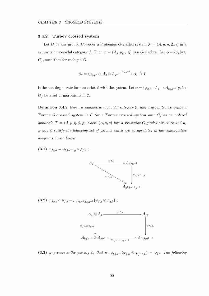
CHAPTER 3. CROSSED SYSTEMS
3.4.2 Turaev crossed system
Let G be any group. Consider a Frobenius G-graded system F = (A,µ, η,∆, ε) in a
symmetric monoidal category C. Then A =(Ag, µg,h, η
)is a G-algebra. Let φ = {φg|g ∈
G}, such that for each g ∈ G,
φg = εµg,g−1 : Ag ⊗Ag−1
µg,g−1
−−−−→ A1ε−→ I
is the non-degenerate form associated with the system. Let ϕ = {ϕg,h : Ag → Ahgh−1 |g, h ∈
G} be a set of morphisms in C.
Definition 3.4.2 Given a symmetric monoidal category C, and a group G, we define a
Turaev G-crossed system in C (or a Turaev crossed system over G) as an ordered
quintuple T = (A,µ, η, φ, ϕ) where (A,µ, η) has a Frobenius G-graded structure and µ,
ϕ and φ satisfy the following set of axioms which are encapsulated in the commutative
diagrams drawn below:
(3.1) ϕf,gh = ϕhfh−1,g ◦ ϕf,h ;
Af
ϕf,gh
&&LLLLLLLLLLLLLLLLLLLLLϕf,h // Ahfh−1
ϕhfh−1,g
��Aghfh−1g−1
(3.2) ϕfg,h ◦ µf,g = µhfh−1,hgh−1
(ϕf,h ⊗ ϕg,h
);
Af ⊗Ag
ϕf,h⊗ϕg,h
��
µf,g // Afg
ϕfg,h
��Ahfh−1 ⊗Ahgh−1
µhfh−1,hgh−1
// Ah(fg)h−1
(3.3) ϕ preserves the pairing φ, that is, φhfh−1(ϕf,h ⊗ ϕf−1,h) = φf . The following
88
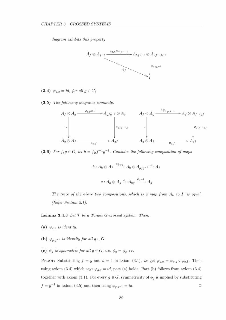
CHAPTER 3. CROSSED SYSTEMS
diagram exhibits this property
Af ⊗Af−1
φf
((QQQQQQQQQQQQQQQQQQQQQQQQQQ
ϕf,h⊗ϕf−1,h // Ahfh−1 ⊗Ahf−1h−1
φhfh−1
��I
(3.4) ϕg,g = id, for all g ∈ G;
(3.5) The following diagrams commute.
Af ⊗Ag
τ
��
ϕf,g⊗1// Agfg−1 ⊗Ag
µgfg−1,g
��Ag ⊗Af µg,f
// Agf
Af ⊗Ag
τ
��
1⊗ϕg,f−1// Af ⊗Af−1gf
µf,f−1gf
��Ag ⊗Af µg,f
// Agf
(3.6) For f, g ∈ G, let h = fgf−1g−1. Consider the following composition of maps
b : Ah ⊗Af1⊗ϕg−−−→ Ah ⊗Agfg−1
µ−→ Af
c : Ah ⊗Agµ−→ Ahg
ϕf−1
−−−→ Ag
The trace of the above two compositions, which is a map from Ah to I, is equal.
(Refer Section 2.1).
Lemma 3.4.3 Let T be a Turaev G-crossed system. Then,
(a) ϕ∗,1 is identity.
(b) ϕg,g−1 is identity for all g ∈ G.
(c) φg is symmetric for all g ∈ G, ı.e. φg = φg−1τ .
Proof: Substituting f = g and h = 1 in axiom (3.1), we get ϕg,g = ϕg,g ◦ ϕg,1. Then
using axiom (3.4) which says ϕg,g = id, part (a) holds. Part (b) follows from axiom (3.4)
together with axiom (3.1). For every g ∈ G, symmetricity of φg is implied by substituting
f = g−1 in axiom (3.5) and then using ϕg,g−1 = id. 2
89
CHAPTER 3. CROSSED SYSTEMS
Note that in case G = 1, Turaev crossed system is simply a Frobenius system (without
grading).
We define a category, T (G) = T (G; C), whose objects are Turaev crossed G-systems
in a symmetric monoidal category C. A morphism T → T ′ in this category is a collection
of morphisms in C mapping each Af to A′f , preserving the unit and the non-degenerate
form associated with the system and commuting with the multiplication and the action
of G. We will need this category only later in the Section 3.5.
3.4.3 K(G,n+1) case
The idea of this subsection and the next section is to give a brief description of the
basic structure of the cobordism category when the target space is a pointed K(G,n+ 1)
space.
Take X to be the Eilenberg-Maclane space K(G,n + 1) for some abelian group G
and n ≥ 1. In this case the objects in X − Cobn are disjoint unions of the chosen
representatives, sayM, where M is a compact manifold without a boundary of dimension
n and we have
[M,X] ∼= Hn+1(M ;G) ∼= 0. (3.8)
Here, [M,X] is the group of all homotopies from M to X. Using the Proposition 3.3.2
we can assume that the characteristic maps of our objects are trivial, that is, they send
everything to the base point x of X. For morphisms A in X − Cobn we have
[A,X ]∂A ∼= [(A, ∂A),X ] ∼= Hn+1((A, ∂A);G). (3.9)
Also we know by Poincare duality,
Hn+1((A, ∂A);G) ∼= H0(A;G). (3.10)
and then by universal coefficient theorem this amounts to H0(A)⊗G. This is nothing
but the connected components of A labelled with elements of G. Thus in this case (n ≥ 1),
X − Cobn is essentially the same category Cobn with labelled components.
90
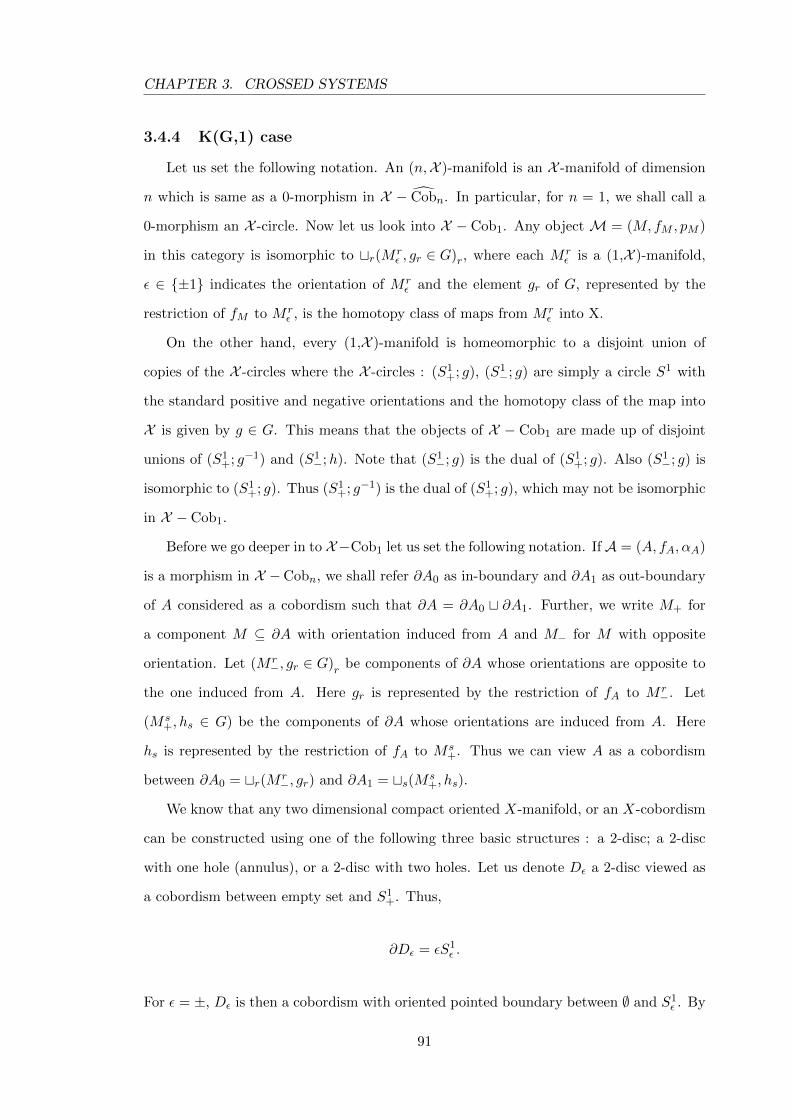
CHAPTER 3. CROSSED SYSTEMS
3.4.4 K(G,1) case
Let us set the following notation. An (n,X )-manifold is an X -manifold of dimension
n which is same as a 0-morphism in X − Cobn. In particular, for n = 1, we shall call a
0-morphism an X -circle. Now let us look into X − Cob1. Any object M = (M,fM , pM )
in this category is isomorphic to tr(M rε , gr ∈ G)r, where each M r
ε is a (1,X )-manifold,
ε ∈ {±1} indicates the orientation of M rε and the element gr of G, represented by the
restriction of fM to M rε , is the homotopy class of maps from M r
ε into X.
On the other hand, every (1,X )-manifold is homeomorphic to a disjoint union of
copies of the X -circles where the X -circles : (S1+; g), (S1
−; g) are simply a circle S1 with
the standard positive and negative orientations and the homotopy class of the map into
X is given by g ∈ G. This means that the objects of X − Cob1 are made up of disjoint
unions of (S1+; g−1) and (S1
−;h). Note that (S1−; g) is the dual of (S1
+; g). Also (S1−; g) is
isomorphic to (S1+; g). Thus (S1
+; g−1) is the dual of (S1+; g), which may not be isomorphic
in X − Cob1.
Before we go deeper in to X−Cob1 let us set the following notation. If A = (A, fA, αA)
is a morphism in X −Cobn, we shall refer ∂A0 as in-boundary and ∂A1 as out-boundary
of A considered as a cobordism such that ∂A = ∂A0 t ∂A1. Further, we write M+ for
a component M ⊆ ∂A with orientation induced from A and M− for M with opposite
orientation. Let (M r−, gr ∈ G)
rbe components of ∂A whose orientations are opposite to
the one induced from A. Here gr is represented by the restriction of fA to M r−. Let
(M s+, hs ∈ G) be the components of ∂A whose orientations are induced from A. Here
hs is represented by the restriction of fA to M s+. Thus we can view A as a cobordism
between ∂A0 = tr(M r−, gr) and ∂A1 = ts(M s
+, hs).
We know that any two dimensional compact oriented X-manifold, or an X-cobordism
can be constructed using one of the following three basic structures : a 2-disc; a 2-disc
with one hole (annulus), or a 2-disc with two holes. Let us denote Dε a 2-disc viewed as
a cobordism between empty set and S1+. Thus,
∂Dε = εS1ε .
For ε = ±, Dε is then a cobordism with oriented pointed boundary between ∅ and S1ε . By
91
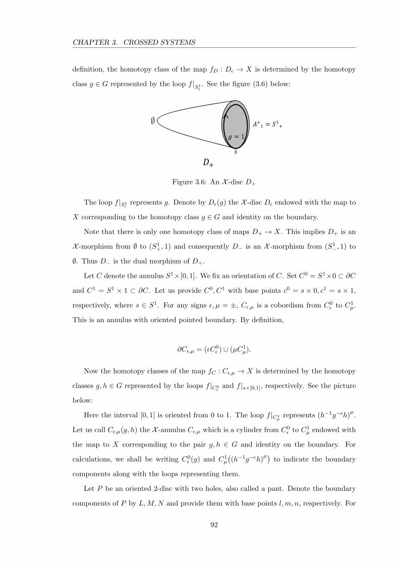
CHAPTER 3. CROSSED SYSTEMS
definition, the homotopy class of the map fD : Dε → X is determined by the homotopy
class g ∈ G represented by the loop f |S1ε. See the figure (3.6) below:
𝑠
𝐷+
𝐴+1 = 𝑆1
+
𝑔 = 1
Figure 3.6: An X -disc D+
The loop f |S1ε
represents g. Denote by Dε(g) the X -disc Dε endowed with the map to
X corresponding to the homotopy class g ∈ G and identity on the boundary.
Note that there is only one homotopy class of maps D+ → X. This implies D+ is an
X -morphism from ∅ to (S1+, 1) and consequently D− is an X -morphism from (S1
−, 1) to
∅. Thus D− is the dual morphism of D+.
Let C denote the annulus S1×[0, 1]. We fix an orientation of C. Set C0 = S1×0 ⊂ ∂C
and C1 = S1 × 1 ⊂ ∂C. Let us provide C0, C1 with base points c0 = s × 0, c1 = s × 1,
respectively, where s ∈ S1. For any signs ε, µ = ±, Cε,µ is a cobordism from C0ε to C1
µ.
This is an annulus with oriented pointed boundary. By definition,
∂Cε,µ = (εC0ε ) ∪ (µC1
µ).
Now the homotopy classes of the map fC : Cε,µ → X is determined by the homotopy
classes g, h ∈ G represented by the loops f |C0ε
and f |s×[0,1], respectively. See the picture
below:
Here the interval [0, 1] is oriented from 0 to 1. The loop f |C1µ
represents (h−1g−εh)µ.
Let us call Cε,µ(g, h) the X -annulus Cε,µ which is a cylinder from C0ε to C1
µ endowed with
the map to X corresponding to the pair g, h ∈ G and identity on the boundary. For
calculations, we shall be writing C0ε (g) and C1
µ
((h−1g−εh)
µ)to indicate the boundary
components along with the loops representing them.
Let P be an oriented 2-disc with two holes, also called a pant. Denote the boundary
components of P by L,M,N and provide them with base points l,m, n, respectively. For
92
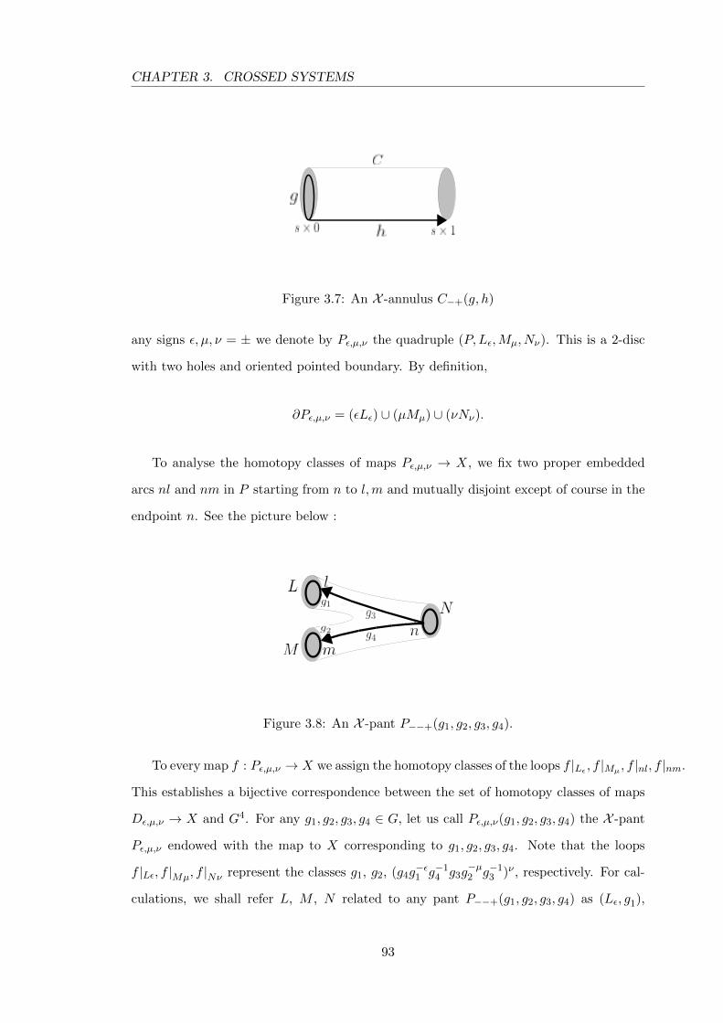
CHAPTER 3. CROSSED SYSTEMS
Figure 3.7: An X -annulus C−+(g, h)
any signs ε, µ, ν = ± we denote by Pε,µ,ν the quadruple (P,Lε,Mµ, Nν). This is a 2-disc
with two holes and oriented pointed boundary. By definition,
∂Pε,µ,ν = (εLε) ∪ (µMµ) ∪ (νNν).
To analyse the homotopy classes of maps Pε,µ,ν → X, we fix two proper embedded
arcs nl and nm in P starting from n to l,m and mutually disjoint except of course in the
endpoint n. See the picture below :
Figure 3.8: An X -pant P−−+(g1, g2, g3, g4).
To every map f : Pε,µ,ν → X we assign the homotopy classes of the loops f |Lε , f |Mµ , f |nl, f |nm.
This establishes a bijective correspondence between the set of homotopy classes of maps
Dε,µ,ν → X and G4. For any g1, g2, g3, g4 ∈ G, let us call Pε,µ,ν(g1, g2, g3, g4) the X -pant
Pε,µ,ν endowed with the map to X corresponding to g1, g2, g3, g4. Note that the loops
f |Lε, f |Mµ, f |Nν represent the classes g1, g2, (g4g−ε1 g−1
4 g3g−µ2 g−1
3 )ν , respectively. For cal-
culations, we shall refer L, M , N related to any pant P−−+(g1, g2, g3, g4) as (Lε, g1),
93
CHAPTER 3. CROSSED SYSTEMS
(Mε, g2) and(Nε, (g4g
−ε1 g−1
4 g3g−µ2 g−1
3 )ν)
respectively to indicate the boundary compo-
nents of the pant along with the loops representing them.
Let us make use of the notation to state the following crucial points about X −Cob1:
(i) The X -circle (S1ε , g) is simply a circle S1
ε with the standard positive or negative
orientation given by ε ∈ {±1} and the homotopy class of the map into X is given
by g ∈ G.
(ii) There are two possible X -discs: D+, D− with D− as the dual of D+ in X − Cob1.
X -cobordism : ∅ → (S1+, 1) with its dual morphism given as D− : (S1
−, 1)→ ∅.
(iii) There are four possible X -annuli Cε,µ(g1, g2) for ε, µ ∈ {±} which are cylinders from
(S1ε ; g1) to (S1
ε,µ; (g−12 g−ε1 g2)µ). Thus we have :
• C−+(g, 1) : (S1−, g)→ (S1
+, g)/C+−(g, 1) : (S1
+, g)→ (S1−, g).
• C−−(g, 1) : (S1−, g) t (S1
−, g−1)→ ∅.
• C++(g−1, 1) : ∅ → (S1+, g
−1) t (S1+, g).
(iv) There are eight possible X -pants for different values of ε, µ, ν ∈ {±} which are cobor-
disms with boundaries in {L =(S1ε , g1
),M =
(S1µ, g2
), N =
(S1ν , (g3g
−ε1 g−1
3 g4g−µ2 g−1
4 )ν)}.
Some basic ones as:
• P−−+(g, h, 1, 1) : (S1−; g) t (S1
−;h)→ (S1+; gh).
• P−−−(g, h, 1, 1) : (S1−; g) t (S1
−;h) t (S1−; k)→ ∅, where k = (gh)−1
These morphisms mentioned above are the basic morphisms that generate the whole
of the category X − Cob1.
Let us denote (S1−; g) as Ag, and the collection (Ag)g∈G as A. We call the collection A
as circles in X −Cob1. Note that since (S1+, g) ∼= (−S1
−, g) in X −Cob1, thus C−+(g, 1) is
essentially identity morphism of Ag. We denote it as 1g : Ag → Ag. For each g ∈ G, let us
set A∗g = (S1−; g−1) and let A∗ = {(Ag−1)∗ : g ∈ G}. Then for each g ∈ G Ag is isomorphic
to (Ag−1)∗. Thus A is isomorphic to A∗ in X − Cob1. Now the X -pant P−−+(f, g, 1, 1)
is an X -morphism in X − Cob1 between L ∪M and N where L = (S1−, f), M = (S1
−, g)
94
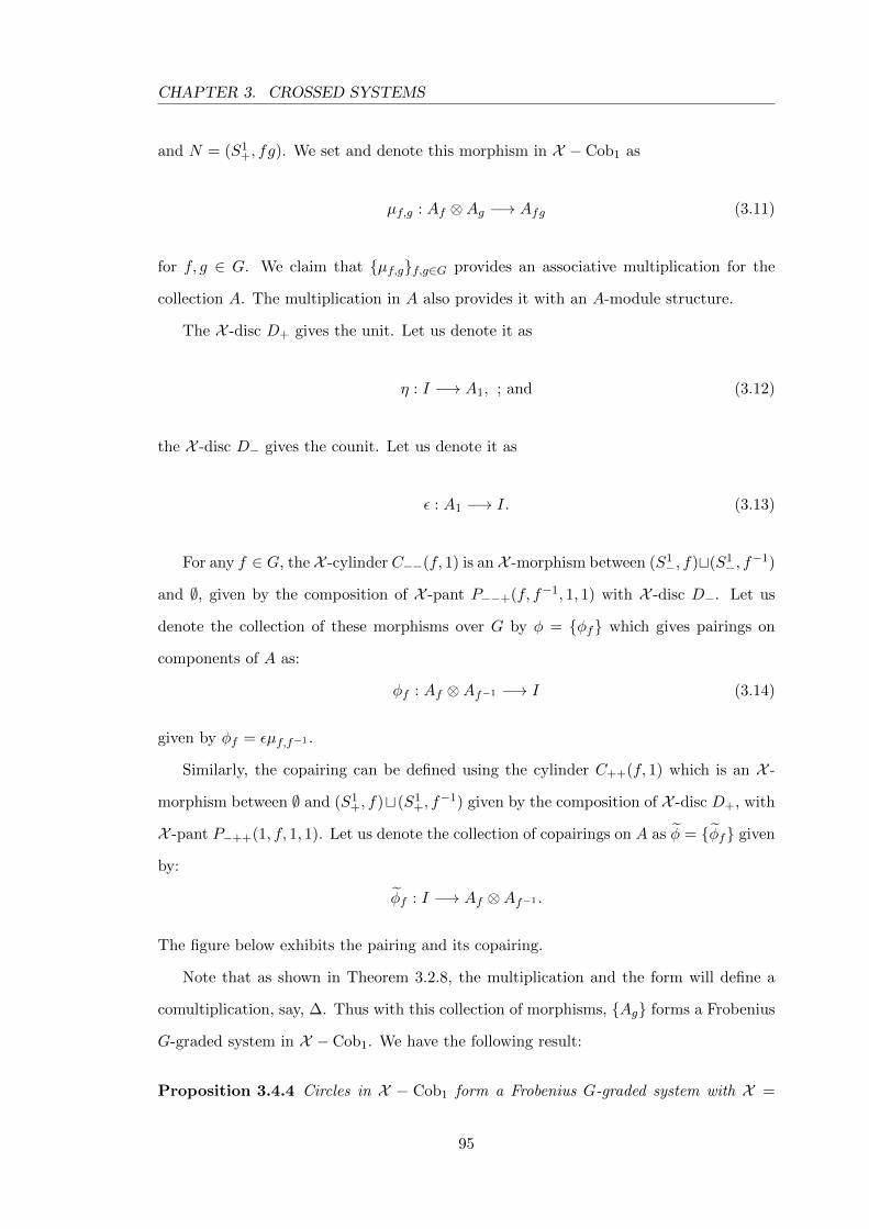
CHAPTER 3. CROSSED SYSTEMS
and N = (S1+, fg). We set and denote this morphism in X − Cob1 as
µf,g : Af ⊗Ag −→ Afg (3.11)
for f, g ∈ G. We claim that {µf,g}f,g∈G provides an associative multiplication for the
collection A. The multiplication in A also provides it with an A-module structure.
The X -disc D+ gives the unit. Let us denote it as
η : I −→ A1, ; and (3.12)
the X -disc D− gives the counit. Let us denote it as
ε : A1 −→ I. (3.13)
For any f ∈ G, the X -cylinder C−−(f, 1) is an X -morphism between (S1−, f)t(S1
−, f−1)
and ∅, given by the composition of X -pant P−−+(f, f−1, 1, 1) with X -disc D−. Let us
denote the collection of these morphisms over G by φ = {φf} which gives pairings on
components of A as:
φf : Af ⊗Af−1 −→ I (3.14)
given by φf = εµf,f−1 .
Similarly, the copairing can be defined using the cylinder C++(f, 1) which is an X -
morphism between ∅ and (S1+, f)t(S1
+, f−1) given by the composition of X -disc D+, with
X -pant P−++(1, f, 1, 1). Let us denote the collection of copairings on A as φ = {φf} given
by:
φf : I −→ Af ⊗Af−1 .
The figure below exhibits the pairing and its copairing.
Note that as shown in Theorem 3.2.8, the multiplication and the form will define a
comultiplication, say, ∆. Thus with this collection of morphisms, {Ag} forms a Frobenius
G-graded system in X − Cob1. We have the following result:
Proposition 3.4.4 Circles in X − Cob1 form a Frobenius G-graded system with X =
95
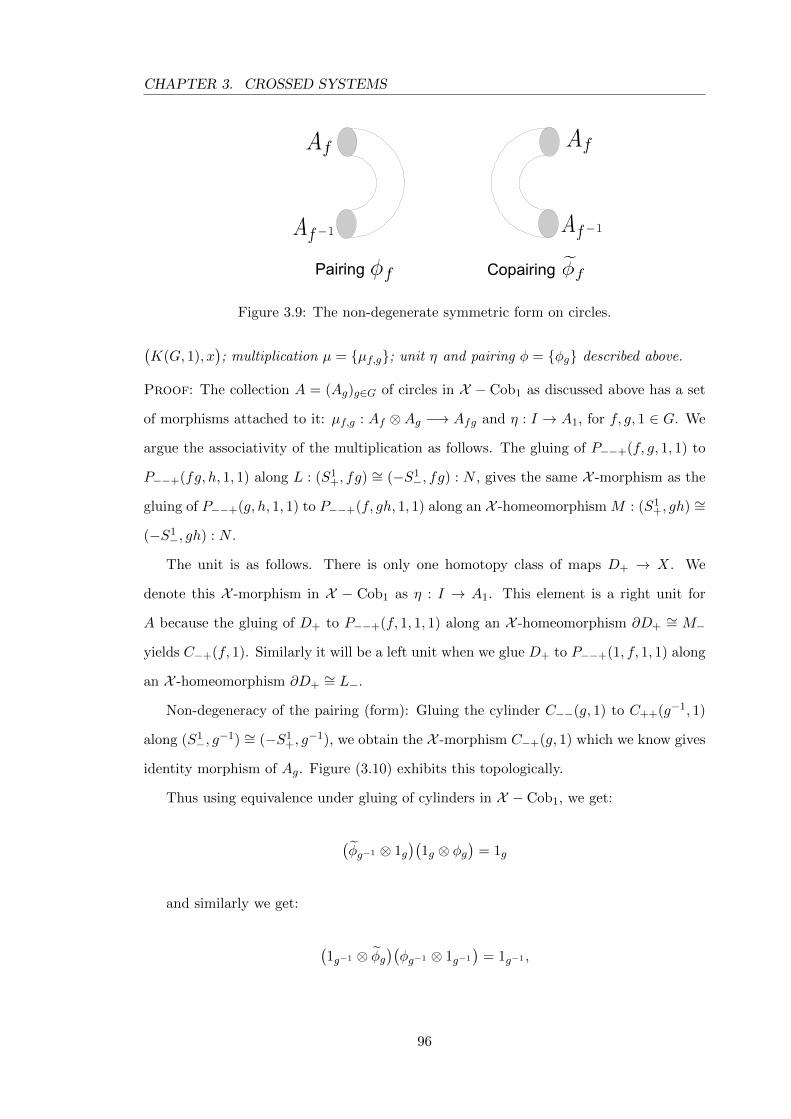
CHAPTER 3. CROSSED SYSTEMS
Pairing Copairing
Figure 3.9: The non-degenerate symmetric form on circles.
(K(G, 1), x
); multiplication µ = {µf,g}; unit η and pairing φ = {φg} described above.
Proof: The collection A = (Ag)g∈G of circles in X − Cob1 as discussed above has a set
of morphisms attached to it: µf,g : Af ⊗ Ag −→ Afg and η : I → A1, for f, g, 1 ∈ G. We
argue the associativity of the multiplication as follows. The gluing of P−−+(f, g, 1, 1) to
P−−+(fg, h, 1, 1) along L : (S1+, fg) ∼= (−S1
−, fg) : N , gives the same X -morphism as the
gluing of P−−+(g, h, 1, 1) to P−−+(f, gh, 1, 1) along an X -homeomorphism M : (S1+, gh) ∼=
(−S1−, gh) : N .
The unit is as follows. There is only one homotopy class of maps D+ → X. We
denote this X -morphism in X − Cob1 as η : I → A1. This element is a right unit for
A because the gluing of D+ to P−−+(f, 1, 1, 1) along an X -homeomorphism ∂D+∼= M−
yields C−+(f, 1). Similarly it will be a left unit when we glue D+ to P−−+(1, f, 1, 1) along
an X -homeomorphism ∂D+∼= L−.
Non-degeneracy of the pairing (form): Gluing the cylinder C−−(g, 1) to C++(g−1, 1)
along (S1−, g
−1) ∼= (−S1+, g
−1), we obtain the X -morphism C−+(g, 1) which we know gives
identity morphism of Ag. Figure (3.10) exhibits this topologically.
Thus using equivalence under gluing of cylinders in X − Cob1, we get:
(φg−1 ⊗ 1g
)(1g ⊗ φg
)= 1g
and similarly we get:
(1g−1 ⊗ φg
)(φg−1 ⊗ 1g−1
)= 1g−1 ,
96
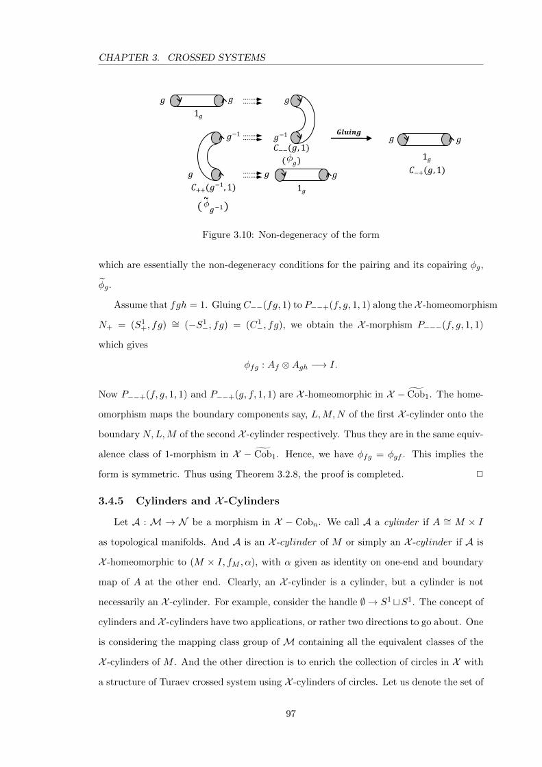
CHAPTER 3. CROSSED SYSTEMS
𝑔
𝑔−1
𝐶−−(𝑔, 1)
( 𝑔)
𝑔 𝑔
𝑔
𝑔−1
𝐶++(𝑔−1, 1)
( 𝑔−1)
)
1𝑔
1𝑔
𝐶−+(𝑔, 1)
𝑔
𝑔
1𝑔
𝑔
𝑔
𝑮𝒍𝒖𝒊𝒏𝒈
Figure 3.10: Non-degeneracy of the form
which are essentially the non-degeneracy conditions for the pairing and its copairing φg,
φg.
Assume that fgh = 1. Gluing C−−(fg, 1) to P−−+(f, g, 1, 1) along the X -homeomorphism
N+ = (S1+, fg) ∼= (−S1
−, fg) = (C1−, fg), we obtain the X -morphism P−−−(f, g, 1, 1)
which gives
φfg : Af ⊗Agh −→ I.
Now P−−+(f, g, 1, 1) and P−−+(g, f, 1, 1) are X -homeomorphic in X − Cob1. The home-
omorphism maps the boundary components say, L,M,N of the first X -cylinder onto the
boundary N,L,M of the second X -cylinder respectively. Thus they are in the same equiv-
alence class of 1-morphism in X − Cob1. Hence, we have φfg = φgf . This implies the
form is symmetric. Thus using Theorem 3.2.8, the proof is completed. 2
3.4.5 Cylinders and X -Cylinders
Let A : M → N be a morphism in X − Cobn. We call A a cylinder if A ∼= M × I
as topological manifolds. And A is an X -cylinder of M or simply an X -cylinder if A is
X -homeomorphic to (M × I, fM , α), with α given as identity on one-end and boundary
map of A at the other end. Clearly, an X -cylinder is a cylinder, but a cylinder is not
necessarily an X -cylinder. For example, consider the handle ∅ → S1tS1. The concept of
cylinders and X -cylinders have two applications, or rather two directions to go about. One
is considering the mapping class group of M containing all the equivalent classes of the
X -cylinders of M . And the other direction is to enrich the collection of circles in X with
a structure of Turaev crossed system using X -cylinders of circles. Let us denote the set of
97
CHAPTER 3. CROSSED SYSTEMS
representatives of equivalence classes of 1-morphisms between M and K as Hom(M,K),
then AΨ ∈ Hom(M,K) and proposition (3.3.1) implies that AΨ and AΦ represent the
same element in Hom(M,K) when Ψ and Φ are isotopic. Note that Aψ ∈ Hom(M,M),
when ψ is a self X -homeomorphism of M.
Let HomeoX (M) be the group of self X -homeomorphisms of M with compact open
topology. Let HomeoX0 (M) be the subset of HomeoX (M) consisting of all X -homeomorphisms
isotopic to the identity morphism on M. It is easy to verify that HomeoX0 (M) is in fact
a normal open subgroup in HomeoX (M). The factor group
MCGX (M) = HomeoX (M)/HomeoX0 (M)
is the mapping class group of M. The elements of this group are the isotopy classes of
self X -homeomorphisms ofM. Note that X -cylinders define a semigroup homomorphism
from MCGX (M) to Hom(M,M) given by [ψ] 7→ Aψ and the composition is given by :
[ψ ◦ φ] 7→ Aψ◦φ = Aψ ◦ Aφ.
Let us now work in the other direction to provide the circles with a structure of a
Turaev G-crossed system.
Using these morphisms, we conclude the section with the following result:
Theorem 3.4.5 Let G be a group and X a K(G; 1) space. Then in X −Cob1, cylinders
define a Turaev G-crossed system on circles.
Proof: We have discussed in the Proposition 3.4.4 that circles form a Frobenius G-
graded system in X − Cob1. The cylinder C−−(g, 1) defines a form φg : Ag ⊗ Ag−1 −→ I
on circles. The information of G-action on circles is carried by the cylinder C−+(g,h−1),
ı.e.
φg : Ag ⊗Ag−1C−−(g,1)−−−−−−→ I
ϕg,h : AgC−+(g,h−1)−−−−−−−→ Ahgh−1
We show the axioms of a Turaev crossed system in the following seven easy steps:
(i) ϕf,gh = ϕhfh−1,g ◦ ϕf,h is depicted in Figure 3.11. Observe that the gluing of
C−+(g, h−1) to C−+(hgh−1, k−1) yields C−+(g, (kh)−1). Then the axiom holds true
98
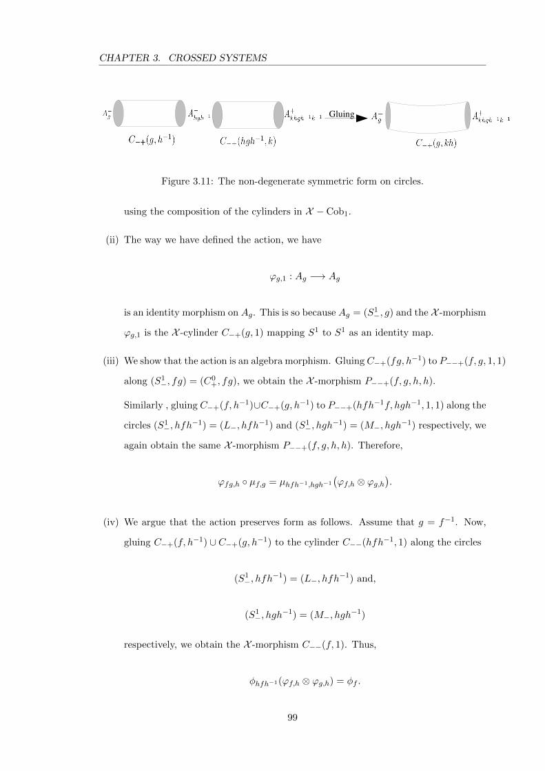
CHAPTER 3. CROSSED SYSTEMS
Gluing
Figure 3.11: The non-degenerate symmetric form on circles.
using the composition of the cylinders in X − Cob1.
(ii) The way we have defined the action, we have
ϕg,1 : Ag −→ Ag
is an identity morphism on Ag. This is so because Ag = (S1−, g) and the X -morphism
ϕg,1 is the X -cylinder C−+(g, 1) mapping S1 to S1 as an identity map.
(iii) We show that the action is an algebra morphism. Gluing C−+(fg, h−1) to P−−+(f, g, 1, 1)
along (S1−, fg) = (C0
+, fg), we obtain the X -morphism P−−+(f, g, h, h).
Similarly , gluing C−+(f, h−1)∪C−+(g, h−1) to P−−+(hfh−1f, hgh−1, 1, 1) along the
circles (S1−, hfh
−1) = (L−, hfh−1) and (S1
−, hgh−1) = (M−, hgh
−1) respectively, we
again obtain the same X -morphism P−−+(f, g, h, h). Therefore,
ϕfg,h ◦ µf,g = µhfh−1,hgh−1
(ϕf,h ⊗ ϕg,h
).
(iv) We argue that the action preserves form as follows. Assume that g = f−1. Now,
gluing C−+(f, h−1) ∪ C−+(g, h−1) to the cylinder C−−(hfh−1, 1) along the circles
(S1−, hfh
−1) = (L−, hfh−1) and,
(S1−, hgh
−1) = (M−, hgh−1)
respectively, we obtain the X -morphism C−−(f, 1). Thus,
φhfh−1(ϕf,h ⊗ ϕg,h) = φf .
99
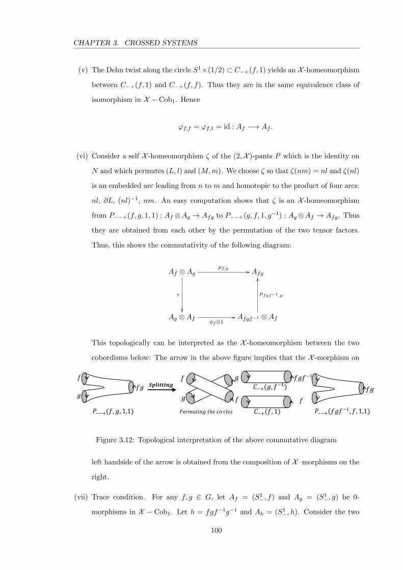
CHAPTER 3. CROSSED SYSTEMS
(v) The Dehn twist along the circle S1×(1/2) ⊂ C−+(f, 1) yields an X -homeomorphism
between C−+(f, 1) and C−+(f, f). Thus they are in the same equivalence class of
isomorphism in X − Cob1. Hence
ϕf,f = ϕf,1 = id : Af −→ Af .
(vi) Consider a self X -homeomorphism ζ of the (2,X )-pants P which is the identity on
N and which permutes (L, l) and (M,m). We choose ζ so that ζ(nm) = nl and ζ(nl)
is an embedded arc leading from n to m and homotopic to the product of four arcs:
nl, ∂L, (nl)−1, nm. An easy computation shows that ζ is an X -homeomorphism
from P−−+(f, g, 1, 1) : Af ⊗Ag → Afg to P−−+(g, f, 1, g−1) : Ag⊗Af → Afg. Thus
they are obtained from each other by the permutation of the two tensor factors.
Thus, this shows the commutativity of the following diagram:
Af ⊗Agµf,g //
τ
��
Afg
Ag ⊗Afφf⊗1
// Afgf−1 ⊗Af
µfgf−1,g
OO
This topologically can be interpreted as the X -homeomorphism between the two
cobordisms below: The arrow in the above figure implies that the X -morphism on
𝑓𝑔 𝑓𝑔
𝑔
𝑓
𝐶−+(𝑓, 1) 𝑃−−+(𝑓,𝑔, 1,1) 𝑃−−+(𝑓𝑔𝑓−1 , 𝑓, 1,1) 𝑃𝑒𝑟𝑚𝑢𝑡𝑖𝑛𝑔 𝑡𝑒 𝑐𝑖𝑟𝑐𝑙𝑒𝑠
𝑓𝑔𝑓−1
𝑓
𝑓
𝑔 𝐶−+(𝑔, 𝑓−1) 𝑺𝒑𝒍𝒊𝒕𝒕𝒊𝒏𝒈
𝑓
𝑔
Figure 3.12: Topological interpretation of the above commutative diagram
left handside of the arrow is obtained from the composition of X–morphisms on the
right.
(vii) Trace condition. For any f, g ∈ G, let Af = (S1−, f) and Ag = (S1
−, g) be 0-
morphisms in X − Cob1. Let h = fgf−1g−1 and Ah = (S1−, h). Consider the two
100
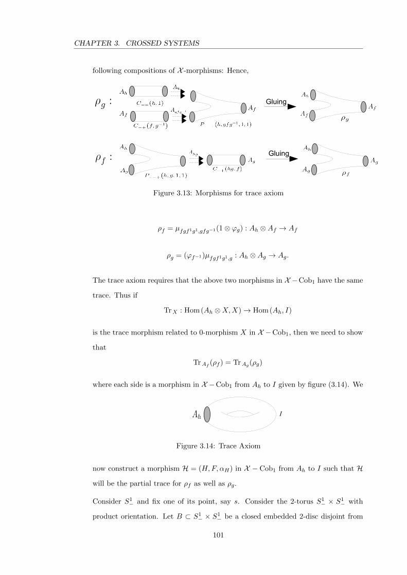
CHAPTER 3. CROSSED SYSTEMS
following compositions of X -morphisms: Hence,
Gluing
Gluing
Figure 3.13: Morphisms for trace axiom
ρf = µfgf1g1,gfg−1(1⊗ ϕg) : Ah ⊗Af → Af
ρg = (ϕf−1)µfgf1g1,g : Ah ⊗Ag → Ag.
The trace axiom requires that the above two morphisms in X −Cob1 have the same
trace. Thus if
TrX : Hom(Ah ⊗X,X)→ Hom(Ah, I)
is the trace morphism related to 0-morphism X in X −Cob1, then we need to show
that
TrAf (ρf ) = TrAg(ρg)
where each side is a morphism in X −Cob1 from Ah to I given by figure (3.14). We
I
Figure 3.14: Trace Axiom
now construct a morphism H = (H,F, αH) in X − Cob1 from Ah to I such that H
will be the partial trace for ρf as well as ρg.
Consider S1− and fix one of its point, say s. Consider the 2-torus S1
− × S1− with
product orientation. Let B ⊂ S1− × S1
− be a closed embedded 2-disc disjoint from
101
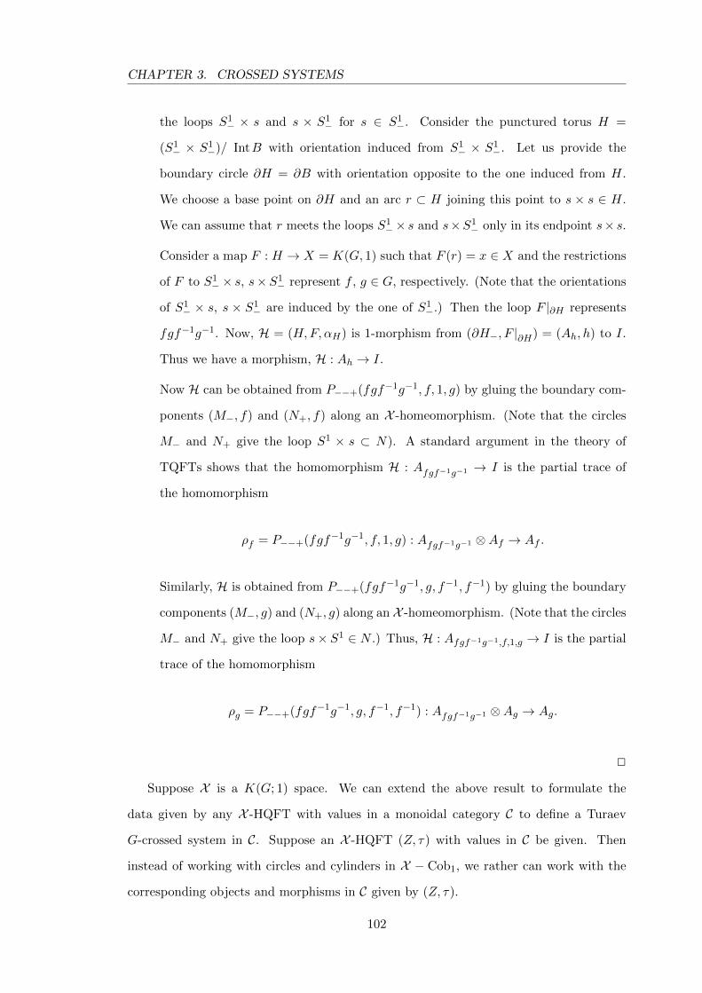
CHAPTER 3. CROSSED SYSTEMS
the loops S1− × s and s × S1
− for s ∈ S1−. Consider the punctured torus H =
(S1− × S1
−)/ IntB with orientation induced from S1− × S1
−. Let us provide the
boundary circle ∂H = ∂B with orientation opposite to the one induced from H.
We choose a base point on ∂H and an arc r ⊂ H joining this point to s × s ∈ H.
We can assume that r meets the loops S1−× s and s×S1
− only in its endpoint s× s.
Consider a map F : H → X = K(G, 1) such that F (r) = x ∈ X and the restrictions
of F to S1−× s, s×S1
− represent f , g ∈ G, respectively. (Note that the orientations
of S1− × s, s × S1
− are induced by the one of S1−.) Then the loop F |∂H represents
fgf−1g−1. Now, H = (H,F, αH) is 1-morphism from (∂H−, F |∂H) = (Ah, h) to I.
Thus we have a morphism, H : Ah → I.
Now H can be obtained from P−−+(fgf−1g−1, f, 1, g) by gluing the boundary com-
ponents (M−, f) and (N+, f) along an X -homeomorphism. (Note that the circles
M− and N+ give the loop S1 × s ⊂ N). A standard argument in the theory of
TQFTs shows that the homomorphism H : Afgf−1g−1 → I is the partial trace of
the homomorphism
ρf = P−−+(fgf−1g−1, f, 1, g) : Afgf−1g−1 ⊗Af → Af .
Similarly, H is obtained from P−−+(fgf−1g−1, g, f−1, f−1) by gluing the boundary
components (M−, g) and (N+, g) along an X -homeomorphism. (Note that the circles
M− and N+ give the loop s× S1 ∈ N .) Thus, H : Afgf−1g−1,f,1,g → I is the partial
trace of the homomorphism
ρg = P−−+(fgf−1g−1, g, f−1, f−1) : Afgf−1g−1 ⊗Ag → Ag.
2
Suppose X is a K(G; 1) space. We can extend the above result to formulate the
data given by any X -HQFT with values in a monoidal category C to define a Turaev
G-crossed system in C. Suppose an X -HQFT (Z, τ) with values in C be given. Then
instead of working with circles and cylinders in X − Cob1, we rather can work with the
corresponding objects and morphisms in C given by (Z, τ).
102
CHAPTER 3. CROSSED SYSTEMS
Observe first that a 1-dimensional connected X -manifoldM is just a pointed oriented
circle endowed with a map into X sending the base point into x. This is nothing but a
loop in X with endpoints in x. If ZM is the object in C given by (Z, τ) corresponding to
M, then clearly it depends only on the class of the loop in π1(X ) = G. Thus for each
g ∈ G, we obtain an object Ag in C.
Recall from Section (3.4.3), where we set our notation as Ag for (S1−; g). Instead (or,
by abuse of notation), we have now set Ag as an object in C given by a X -HQFT (Z, τ)
which corresponds to a 1-dimensional connected X -manifold M which depends only on
the class g of the loop in G. Thus we have a collection A = {Ag} of objects in C. The
X -HQFT sends X -cobordisms to morphisms in C. Then, as in equations (3.11) to (3.14),
we have the morphisms
µf,g : Af ⊗Ag → Afg
η : IC → A1
ε : A1 → IC
φf : Af ⊗Af−1 → I
in C which equips the collection A = {Ag} with a Frobenius structure (Proposition 3.4.3).
Further, the calculations done in Theorem (3.4.4) are exactly the same so as to endow the
Frobenius system A = {Ag} with a Turaev structure. Thus the X -HQFT (Z, τ) defines a
Turaev G-crossed system A = {Ag} in C. We can summarise this discussion in the form
of the following result:
Theorem 3.4.6 Suppose X is a K(G; 1) space. Then any (1+1)-dimensional X -HQFT
with values in C defines a Turaev G-crossed system in C.
3.5 HQFTs
Assume (S,⊗, I) to be a symmetric monoidal category. Consider a Turaev crossed
system A = (Ag, µ, η, φ, ϕ) in S. Let (Z, τ) be a (1+1)-dimensional HQFT over K(G, 1)
space with values in S. The aim of this section is to reconstruct (Z, τ)(at least up to
isomorphism) from an underlying Turaev crossed system A. Throughout this section we
103
CHAPTER 3. CROSSED SYSTEMS
shall use the term X -surface for the base space of any X -morphism in X − Cob1.
3.5.1 Computing τ
In this section we compute the morphisms (values of τ) for (1+1)-dimensional X -
HQFT (Z, τ) when the underlying Turaev G-crossed system A is given to us.
It follows from the topological classification of surfaces that every compact oriented
surface can be split along a finite set of disjoint simple loops into a union of discs with ≤ 2
holes, ı.e., discs, annuli and discs with two holes. This implies that every X -surface W
can be obtained by gluing from a finite collection of X -surfaces which are discs with ≤ 2
holes. Axioms of an HQFT imply that morphism τ(W ) in S is determined by the values
of τ on the discs with ≤ 2 holes. We show that these values are completely determined
by A.
We begin by computing τ for X -annuli. Each X -annulus is isomorphic to one of these:
• C−+(g, h) or C+−(g, h)
• C−−(g, h)
• C++(g, h)
We define,
τ(C−+(g, h)
):= ϕg,h−1 : Ag → Ah−1gh and (3.15)
τ(C−−(g, 1)
):= φg : Ag ⊗Ag−1 → I.
The X -annulus C−−(g, h) can be obtained by the gluing of two X -annuli C−+(g, h)
and C−−(h−1gh, 1) along (S1+, h
−1gh) = (S1−, h
−1gh). Algebraically, we have the following
composition of morphisms in the category S:
Ag ⊗Ah−1g−1h
ϕg,h−1⊗1−−−−−−→ Ah−1gh ⊗Ah−1g−1h
φh−1gh−−−−→ I.
which helps us to define:
τ(C−−(g;h) = φh−1gh(ϕg,h−1 ⊗ 1) : Ag ⊗Ah−1g−1h → I. (3.16)
Note that here we make use of the gluing process in X − Cob1 which corresponds to
104
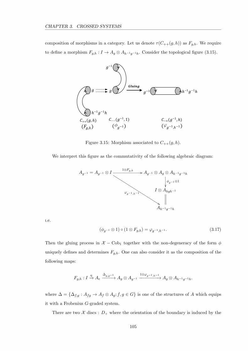
CHAPTER 3. CROSSED SYSTEMS
composition of morphisms in a category. Let us denote τ(C++(g, h)) as Fg,h. We require
to define a morphism Fg,h : I → Ag ⊗Ah−1g−1h. Consider the topological figure (3.15).
ℎ−1𝑔−1ℎ
ℎ−1𝑔−1ℎ
𝑔 𝑔−1
𝑮𝒍𝒖𝒊𝒏𝒈
𝑔−1
𝑔
𝐶++(𝑔, ℎ)
(𝐹𝑔,ℎ)
𝐶−−(𝑔−1, 1)
( 𝑔−1)
𝐶−+(𝑔−1, ℎ)
( 𝑔−1 ,ℎ−1)
Figure 3.15: Morphism associated to C++(g, h).
We interpret this figure as the commutativity of the following algebraic diagram:
Ag−1 = Ag−1 ⊗ I
ϕg−1,h−1
%%KKKKKKKKKKKKKKKKKKKKKKKKKKK1⊗Fg,h // Ag−1 ⊗Ag ⊗Ah−1g−1h
φg−1⊗1
��I ⊗Ahgh−1
Ah−1g−1h
ı.e.
(φg−1 ⊗ 1) ◦ (1⊗ Fg,h) = ϕg−1,h−1 . (3.17)
Then the gluing process in X − Cob1 together with the non-degeneracy of the form φ
uniquely defines and determines Fg,h. One can also consider it as the composition of the
following maps:
Fg,h : Iη−→ Ae
∆g,g−1
−−−−→ Ag ⊗Ag−1
1⊗ϕg−1,h−1
−−−−−−−−→ Ag ⊗Ah−1g−1h.
where ∆ = {∆f,g : Afg → Af ⊗ Ag; f, g ∈ G} is one of the structures of A which equips
it with a Frobenius G-graded system.
There are two X discs : D+ where the orientation of the boundary is induced by the
105
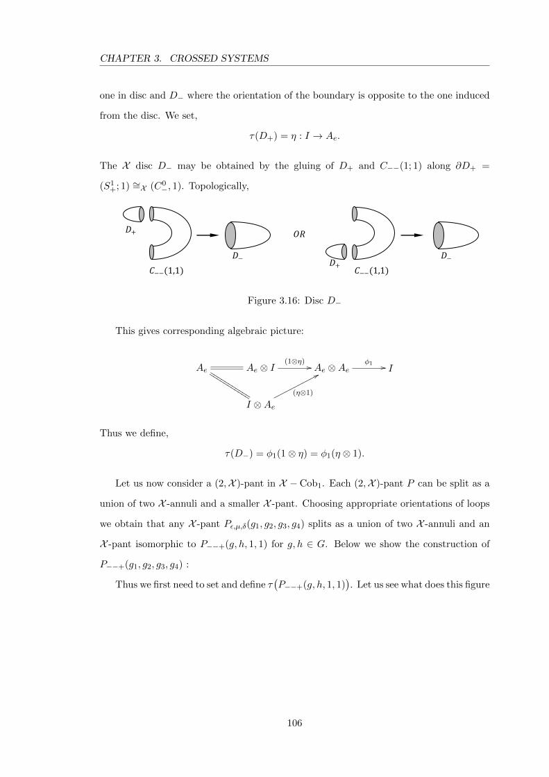
CHAPTER 3. CROSSED SYSTEMS
one in disc and D− where the orientation of the boundary is opposite to the one induced
from the disc. We set,
τ(D+) = η : I → Ae.
The X disc D− may be obtained by the gluing of D+ and C−−(1; 1) along ∂D+ =
(S1+; 1) ∼=X (C0
−, 1). Topologically,
𝐶−−(1,1)
𝐷+
𝐷− 𝐷+
𝐶−−(1,1)
𝐷−
𝑂𝑅
Figure 3.16: Disc D−
This gives corresponding algebraic picture:
Ae
KKKKKKKKKKK
KKKKKKKKKKK Ae ⊗ I(1⊗η) // Ae ⊗Ae
φ1 // I
I ⊗Ae(η⊗1)
77ppppppppppp
Thus we define,
τ(D−) = φ1(1⊗ η) = φ1(η ⊗ 1).
Let us now consider a (2,X )-pant in X −Cob1. Each (2,X )-pant P can be split as a
union of two X -annuli and a smaller X -pant. Choosing appropriate orientations of loops
we obtain that any X -pant Pε,µ,δ(g1, g2, g3, g4) splits as a union of two X -annuli and an
X -pant isomorphic to P−−+(g, h, 1, 1) for g, h ∈ G. Below we show the construction of
P−−+(g1, g2, g3, g4) :
Thus we first need to set and define τ(P−−+(g, h, 1, 1)
). Let us see what does this figure
106
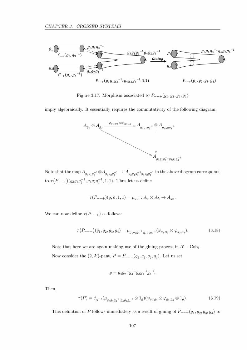
CHAPTER 3. CROSSED SYSTEMS
𝑔3𝑔1𝑔3−1𝑔4𝑔2𝑔4
−1
𝑔3𝑔1𝑔3−1𝑔4𝑔2𝑔4
−1
𝑔4𝑔2𝑔4−1
𝑔1
𝑔2
𝑔3𝑔1𝑔3−1
𝐶−+(𝑔1,𝑔3−1)
𝐶−+(𝑔2,𝑔4−1)
𝑃−−+(𝑔3𝑔1𝑔3−1 ,𝑔4𝑔2𝑔4
−1, 1,1) 𝑃−−+(𝑔1,𝑔2 ,𝑔3,𝑔4)
𝑮𝒍𝒖𝒊𝒏𝒈
𝑔2
𝑔1
Figure 3.17: Morphism associated to P−−+(g1, g2, g3, g4)
imply algebraically. It essentially requires the commutativity of the following diagram:
Ag1 ⊗Ag2
''OOOOOOOOOOOOOOOOOOOOOOOOOOOO
ϕg1,g3⊗ϕg2,g4 // Ag3g1g
−13
⊗Ag4g2g
−14
��Ag3g1g
−13 g4g2g
−14
Note that the map Ag3g1g−13⊗Ag4g2g−1
4→ Ag3g1g
−13 g4g2g
−14
in the above diagram corresponds
to τ(P−−+
)(g3g1g
−13 , g4g2g
−14 , 1, 1). Thus let us define
τ(P−−+)(g, h, 1, 1) = µg,h : Ag ⊗Ah → Agh.
We can now define τ(P−−+) as follows:
τ(P−−+
)(g1, g2, g3, g4) = µg3g1g
−13 ,g4g2g
−14
(ϕg1,g3 ⊗ ϕg2,g4). (3.18)
Note that here we are again making use of the gluing process in X − Cob1.
Now consider the (2,X )-pant, P = P−−−(g1, g2, g3, g4). Let us set
g = g4g−12 g−1
4 g3g−11 g−1
3 .
Then,
τ(P ) = φg−1(µg3g1g−13 ,g4g2g
−14⊗ 1g)(ϕg1,g3 ⊗ ϕg2,g4 ⊗ 1g). (3.19)
This definition of P follows immediately as a result of gluing of P−−+(g1, g2, g3, g4) to
107
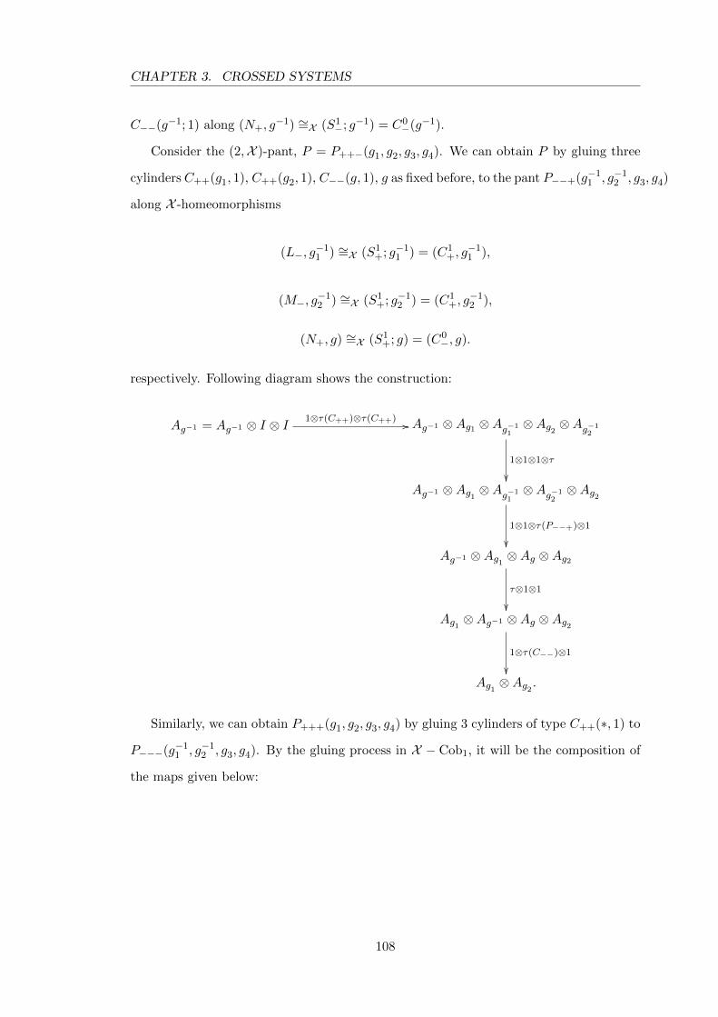
CHAPTER 3. CROSSED SYSTEMS
C−−(g−1; 1) along (N+, g−1) ∼=X (S1
−; g−1) = C0−(g−1).
Consider the (2,X )-pant, P = P++−(g1, g2, g3, g4). We can obtain P by gluing three
cylinders C++(g1, 1), C++(g2, 1), C−−(g, 1), g as fixed before, to the pant P−−+(g−11 , g−1
2 , g3, g4)
along X -homeomorphisms
(L−, g−11 ) ∼=X (S1
+; g−11 ) = (C1
+, g−11 ),
(M−, g−12 ) ∼=X (S1
+; g−12 ) = (C1
+, g−12 ),
(N+, g) ∼=X (S1+; g) = (C0
−, g).
respectively. Following diagram shows the construction:
Ag−1 = Ag−1 ⊗ I ⊗ I 1⊗τ(C++)⊗τ(C++) // Ag−1 ⊗Ag1 ⊗Ag−11⊗Ag2 ⊗Ag−1
2
1⊗1⊗1⊗τ
��Ag−1 ⊗Ag1 ⊗Ag−1
1⊗Ag−1
2⊗Ag2
1⊗1⊗τ(P−−+)⊗1
��Ag−1 ⊗Ag1 ⊗Ag ⊗Ag2
τ⊗1⊗1
��Ag1 ⊗Ag−1 ⊗Ag ⊗Ag2
1⊗τ(C−−)⊗1
��Ag1 ⊗Ag2 .
Similarly, we can obtain P+++(g1, g2, g3, g4) by gluing 3 cylinders of type C++(∗, 1) to
P−−−(g−11 , g−1
2 , g3, g4). By the gluing process in X − Cob1, it will be the composition of
the maps given below:
108
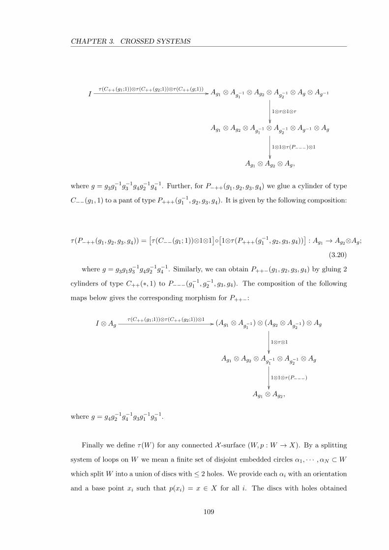
CHAPTER 3. CROSSED SYSTEMS
Iτ(C++(g1;1))⊗τ(C++(g2;1))⊗τ(C++(g;1)) // Ag1 ⊗Ag−1
1⊗Ag2 ⊗Ag−1
2⊗Ag ⊗Ag−1
1⊗τ⊗1⊗τ
��Ag1 ⊗Ag2 ⊗Ag−1
1⊗Ag−1
2⊗Ag−1 ⊗Ag
1⊗1⊗τ(P−−−)⊗1
��Ag1 ⊗Ag2 ⊗Ag,
where g = g3g−11 g−1
3 g4g−12 g−1
4 . Further, for P−++(g1, g2, g3, g4) we glue a cylinder of type
C−−(g1, 1) to a pant of type P+++(g−11 , g2, g3, g4). It is given by the following composition:
τ(P−++(g1, g2, g3, g4)) =[τ(C−−(g1; 1))⊗1⊗1
]◦[1⊗τ(P+++(g−1
1 , g2, g3, g4))]
: Ag1 → Ag2⊗Ag;
(3.20)
where g = g3g1g−13 g4g
−12 g−1
4 . Similarly, we can obtain P++−(g1, g2, g3, g4) by gluing 2
cylinders of type C++(∗, 1) to P−−−(g−11 , g−1
2 , g3, g4). The composition of the following
maps below gives the corresponding morphism for P++−:
I ⊗Agτ(C++(g1;1))⊗τ(C++(g2;1))⊗1 // (Ag1 ⊗Ag−1
1)⊗ (Ag2 ⊗Ag−1
2)⊗Ag
1⊗τ⊗1
��Ag1 ⊗Ag2 ⊗Ag−1
1⊗Ag−1
2⊗Ag
1⊗1⊗τ(P−−−)
��Ag1 ⊗Ag2 ,
where g = g4g−12 g−1
4 g3g−11 g−1
3 .
Finally we define τ(W ) for any connected X -surface (W,p : W → X). By a splitting
system of loops on W we mean a finite set of disjoint embedded circles α1, · · · , αN ⊂ W
which split W into a union of discs with ≤ 2 holes. We provide each αi with an orientation
and a base point xi such that p(xi) = x ∈ X for all i. The discs with holes obtained
109
CHAPTER 3. CROSSED SYSTEMS
by the splitting of W along ∪iαi endowed with the restriction of p are X -surfaces. The
gluing process in X − Cob1 determines τ(W ) from the values of τ on these discs with
holes. Thus, we have defined τ for any connected X -surface. We can then extend τ to
any arbitrary X -surface using the monoidal structure of X − Cob1.
Lemma 3.5.1 The morphisms in S defined in equations (3.15) to (3.20) which corre-
sponds to X -cobordisms are all well defined.
Proof: For the well defineness of the morphisms we need to show the topological invari-
ance of the morphisms under X -homeomorphisms. The X -homeomorphisms of (2,X )-
cylinders are generated by (1) the Dehn twists Cε,µ(g;h) → Cε,µ(g;hg) along the circle
S1×(1/2) where ε, µ = ± and (2) the X -homeomorphisms Cε,ε(g, h)→ Cε,ε(h−1g−1h, h−1)
permuting the boundary components of the cylinder and preserving the arc s× [0, 1] (with
s ∈ S1) as a set. So, to establish the topological invariance for (2,X )-cylinders, it is suf-
fices to check the invariance under these two morphisms.
The invariance of τ under the Dehn twists for C−+ is as follows:
τ(C−+(f, h−1)) = ϕf,h : Af → Ahfh−1
τ(C−+(f, (hg)−1)) = ϕf,hg : Af → Ahfh−1 .
Now, ϕg,hg = (ϕg,h ◦ ϕg,g) = ϕg,h. The following calculation shows the invariance of τ
under Dehn twists for C−− :
τ(C−−(g, hg)
)= φ(hg)g(hg)−1
(ϕg,hg ⊗ 1
)= φhgh−1
(ϕg,h ⊗ 1
)= τ
(C−−(g, h)
).
110
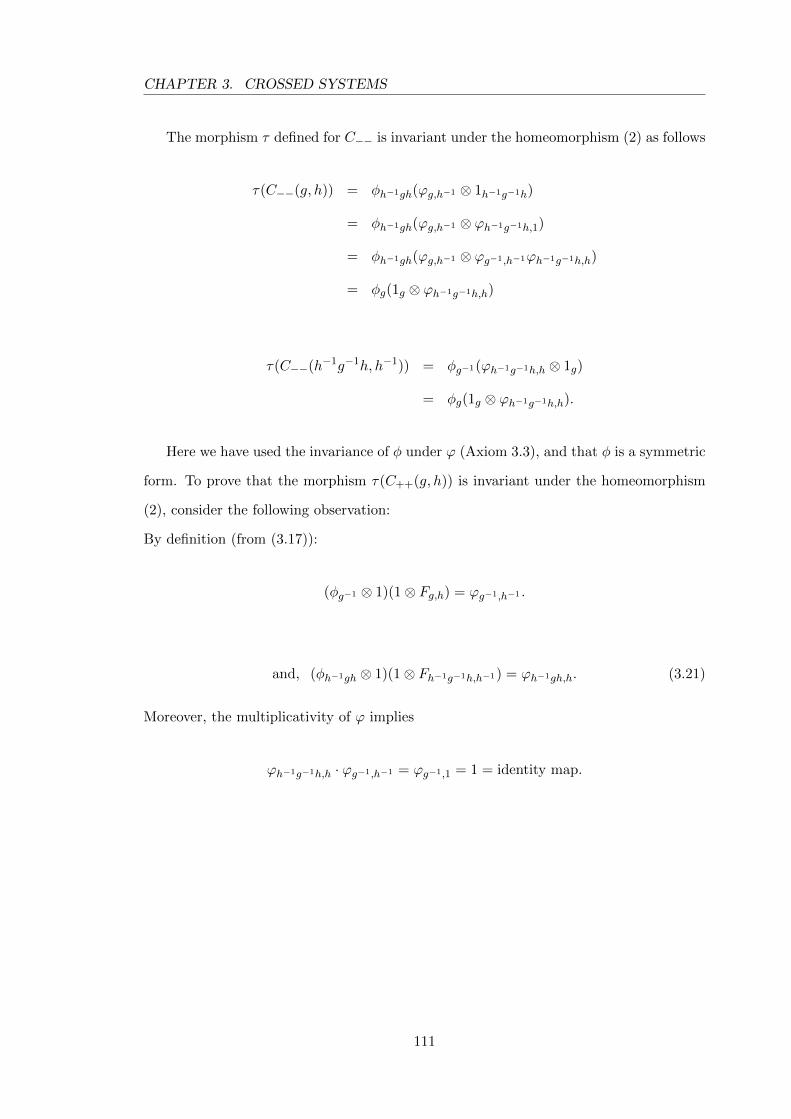
CHAPTER 3. CROSSED SYSTEMS
The morphism τ defined for C−− is invariant under the homeomorphism (2) as follows
τ(C−−(g, h)) = φh−1gh(ϕg,h−1 ⊗ 1h−1g−1h)
= φh−1gh(ϕg,h−1 ⊗ ϕh−1g−1h,1)
= φh−1gh(ϕg,h−1 ⊗ ϕg−1,h−1ϕh−1g−1h,h)
= φg(1g ⊗ ϕh−1g−1h,h)
τ(C−−(h−1g−1h, h−1)) = φg−1(ϕh−1g−1h,h ⊗ 1g)
= φg(1g ⊗ ϕh−1g−1h,h).
Here we have used the invariance of φ under ϕ (Axiom 3.3), and that φ is a symmetric
form. To prove that the morphism τ(C++(g, h)) is invariant under the homeomorphism
(2), consider the following observation:
By definition (from (3.17)):
(φg−1 ⊗ 1)(1⊗ Fg,h) = ϕg−1,h−1 .
and, (φh−1gh ⊗ 1)(1⊗ Fh−1g−1h,h−1) = ϕh−1gh,h. (3.21)
Moreover, the multiplicativity of ϕ implies
ϕh−1g−1h,h · ϕg−1,h−1 = ϕg−1,1 = 1 = identity map.
111
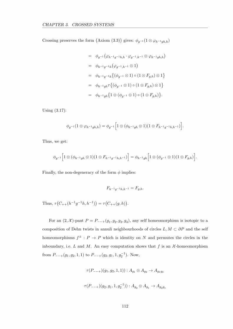
CHAPTER 3. CROSSED SYSTEMS
Crossing preserves the form(Axiom (3.3)
)gives: φg−1(1⊗ ϕh−1gh,h)
= φg−1
(ϕh−1g−1h,h · ϕg−1,h−1 ⊗ ϕh−1gh,h
)= φh−1g−1h
(ϕg−1,h−1 ⊗ 1
)= φh−1g−1h
{(φg−1 ⊗ 1) ◦ (1⊗ Fg,h)⊗ 1
}= φh−1ghτ
{(φg−1 ⊗ 1) ◦ (1⊗ Fg,h)⊗ 1
}= φh−1gh
{1⊗ (φg−1 ⊗ 1) ◦ (1⊗ Fg,h)
}.
Using (3.17):
φg−1(1⊗ ϕh−1gh,h) = φg−1
[1⊗ (φh−1gh ⊗ 1)(1⊗ Fh−1g−1h,h−1)
].
Thus, we get:
φg−1
[1⊗ (φh−1gh ⊗ 1)(1⊗ Fh−1g−1h,h−1)
]= φh−1gh
[1⊗ (φg−1 ⊗ 1)(1⊗ Fg,h)
].
Finally, the non-degeneracy of the form φ implies:
Fh−1g−1h,h−1 = Fg,h.
Thus, τ(C++(h−1g−1h, h−1)
)= τ
(C++(g, h)
).
For an (2,X )-pant P = P−−+(g1, g2, g3, g4), any self homeomorphism is isotopic to a
composition of Dehn twists in annuli neighbourhoods of circles L,M ⊂ ∂P and the self
homeomorphisms f± : P → P which is identity on N and permutes the circles in the
inboundary, i.e. L and M . An easy computation shows that f is an X -homeomorphism
from P−−+(g1, g2, 1, 1) to P−−+(g2, g1, 1, g−12 ). Now,
τ(P−−+)(g1, g2, 1, 1)) : Ag1 ⊗Ag2 → Ag1g2
τ(P−−+)(g2, g1, 1, g−12 )) : Ag2 ⊗Ag1 → Ag2g1
112
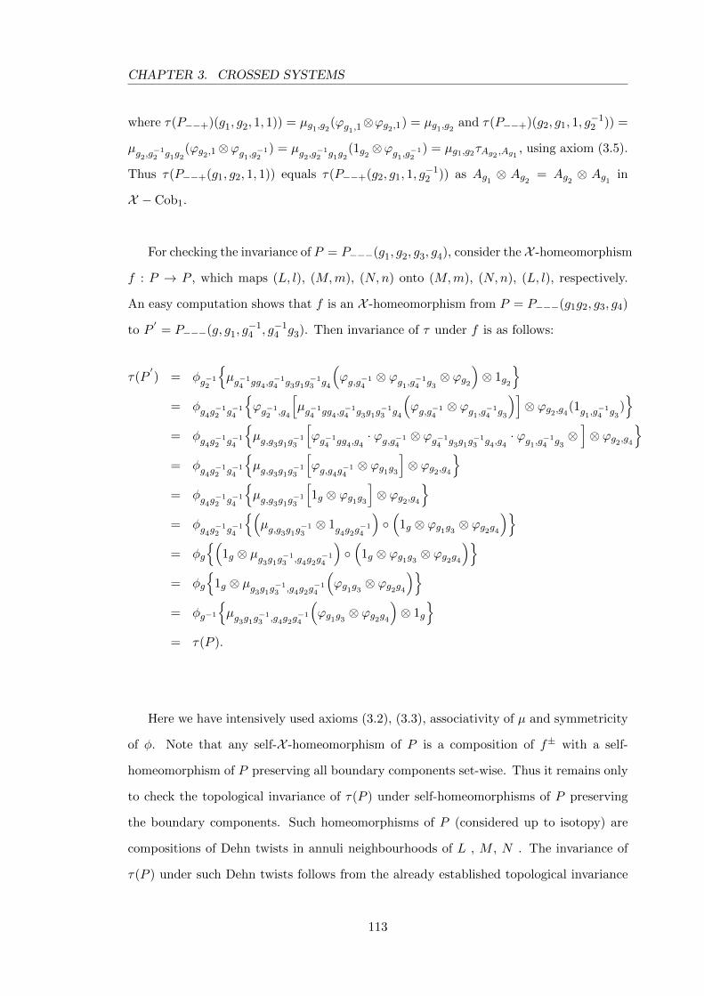
CHAPTER 3. CROSSED SYSTEMS
where τ(P−−+)(g1, g2, 1, 1)) = µg1,g2(ϕg1,1⊗ϕg2,1) = µg1,g2 and τ(P−−+)(g2, g1, 1, g
−12 )) =
µg2,g−12 g1g2
(ϕg2,1⊗ϕg1,g−12
) = µg2,g−12 g1g2
(1g2 ⊗ϕg1,g−12
) = µg1,g2τAg2 ,Ag1 , using axiom (3.5).
Thus τ(P−−+(g1, g2, 1, 1)) equals τ(P−−+(g2, g1, 1, g−12 )) as Ag1 ⊗ Ag2 = Ag2 ⊗ Ag1 in
X − Cob1.
For checking the invariance of P = P−−−(g1, g2, g3, g4), consider the X -homeomorphism
f : P → P , which maps (L, l), (M,m), (N,n) onto (M,m), (N,n), (L, l), respectively.
An easy computation shows that f is an X -homeomorphism from P = P−−−(g1g2, g3, g4)
to P′
= P−−−(g, g1, g−14 , g−1
4 g3). Then invariance of τ under f is as follows:
τ(P′) = φg−1
2
{µg−1
4 gg4,g−14 g3g1g
−13 g4
(ϕg,g−1
4⊗ ϕg1,g−1
4 g3⊗ ϕg2
)⊗ 1g2
}= φg4g
−12 g−1
4
{ϕg−1
2 ,g4
[µg−1
4 gg4,g−14 g3g1g
−13 g4
(ϕg,g−1
4⊗ ϕg1,g−1
4 g3
)]⊗ ϕg2,g4(1g1,g
−14 g3
)}
= φg4g−12 g−1
4
{µg,g3g1g
−13
[ϕg−1
4 gg4,g4· ϕg,g−1
4⊗ ϕg−1
4 g3g1g−13 g4,g4
· ϕg1,g−14 g3⊗]⊗ ϕg2,g4
}= φg4g
−12 g−1
4
{µg,g3g1g
−13
[ϕg,g4g
−14⊗ ϕg1g3
]⊗ ϕg2,g4
}= φg4g
−12 g−1
4
{µg,g3g1g
−13
[1g ⊗ ϕg1g3
]⊗ ϕg2,g4
}= φg4g
−12 g−1
4
{(µg,g3g1g
−13⊗ 1g4g2g
−14
)◦(
1g ⊗ ϕg1g3 ⊗ ϕg2g4)}
= φg
{(1g ⊗ µg3g1g−1
3 ,g4g2g−14
)◦(
1g ⊗ ϕg1g3 ⊗ ϕg2g4)}
= φg
{1g ⊗ µg3g1g−1
3 ,g4g2g−14
(ϕg1g3 ⊗ ϕg2g4
)}= φg−1
{µg3g1g
−13 ,g4g2g
−14
(ϕg1g3 ⊗ ϕg2g4
)⊗ 1g
}= τ(P ).
Here we have intensively used axioms (3.2), (3.3), associativity of µ and symmetricity
of φ. Note that any self-X -homeomorphism of P is a composition of f± with a self-
homeomorphism of P preserving all boundary components set-wise. Thus it remains only
to check the topological invariance of τ(P ) under self-homeomorphisms of P preserving
the boundary components. Such homeomorphisms of P (considered up to isotopy) are
compositions of Dehn twists in annuli neighbourhoods of L , M , N . The invariance of
τ(P ) under such Dehn twists follows from the already established topological invariance
113
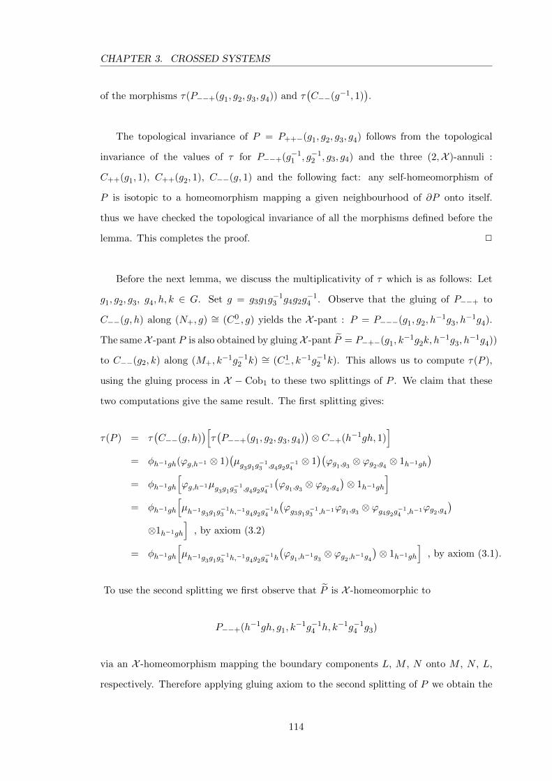
CHAPTER 3. CROSSED SYSTEMS
of the morphisms τ(P−−+(g1, g2, g3, g4)) and τ(C−−(g−1, 1)
).
The topological invariance of P = P++−(g1, g2, g3, g4) follows from the topological
invariance of the values of τ for P−−+(g−11 , g−1
2 , g3, g4) and the three (2,X )-annuli :
C++(g1, 1), C++(g2, 1), C−−(g, 1) and the following fact: any self-homeomorphism of
P is isotopic to a homeomorphism mapping a given neighbourhood of ∂P onto itself.
thus we have checked the topological invariance of all the morphisms defined before the
lemma. This completes the proof. 2
Before the next lemma, we discuss the multiplicativity of τ which is as follows: Let
g1, g2, g3, g4, h, k ∈ G. Set g = g3g1g−13 g4g2g
−14 . Observe that the gluing of P−−+ to
C−−(g, h) along (N+, g) ∼= (C0−, g) yields the X -pant : P = P−−−(g1, g2, h
−1g3, h−1g4).
The same X -pant P is also obtained by gluing X -pant P = P−+−(g1, k−1g2k, h
−1g3, h−1g4))
to C−−(g2, k) along (M+, k−1g−1
2 k) ∼= (C1−, k
−1g−12 k). This allows us to compute τ(P ),
using the gluing process in X − Cob1 to these two splittings of P . We claim that these
two computations give the same result. The first splitting gives:
τ(P ) = τ(C−−(g, h)
)[τ(P−−+(g1, g2, g3, g4)
)⊗ C−+(h−1gh, 1)
]= φh−1gh(ϕg,h−1 ⊗ 1)
(µg3g1g
−13 ,g4g2g
−14⊗ 1)(ϕg1,g3 ⊗ ϕg2,g4 ⊗ 1h−1gh
)= φh−1gh
[ϕg,h−1µg3g1g
−13 ,g4g2g
−14
(ϕg1,g3 ⊗ ϕg2,g4
)⊗ 1h−1gh
]= φh−1gh
[µh−1g3g1g
−13 h,−1g4g2g
−14 h
(ϕg3g1g
−13 ,h−1ϕg1,g3 ⊗ ϕg4g2g−1
4 ,h−1ϕg2,g4)
⊗1h−1gh
], by axiom (3.2)
= φh−1gh
[µh−1g3g1g
−13 h,−1g4g2g
−14 h
(ϕg1,h−1g3
⊗ ϕg2,h−1g4
)⊗ 1h−1gh
], by axiom (3.1).
To use the second splitting we first observe that P is X -homeomorphic to
P−−+(h−1gh, g1, k−1g−1
4 h, k−1g−14 g3)
via an X -homeomorphism mapping the boundary components L, M , N onto M , N , L,
respectively. Therefore applying gluing axiom to the second splitting of P we obtain the
114
CHAPTER 3. CROSSED SYSTEMS
value of τ(P )
= τ(C−−(g2, k)[C−+(k−1g2k, 1)⊗ τ
(P−−+(h−1gh, g1, k
−1g−14 h, k−1g−1
4 g3))]
= φk−1g2k(ϕg2,k−1 ⊗ 1k−1g−1
2 k)[1k−1g2k
⊗ µk−1g−14 g−1g4k,k
−1g−14 g3g1g
−13 g4k(
ϕh−1g−1h,k−1g−14 h ⊗ ϕg1,g−1
4 g3
)]= φk−1g2k
[ϕg2,k−1 ⊗ µk−1g−1
4 g−1g4k,k−1g−1
4 g3g1g−13 g4k(
ϕg−14 g−1g4,k
−1ϕh−1g−1h,g−14 h ⊗ ϕg−1
4 g3g1g−13 g4,k
−1ϕg1,g−14 g3
)]= φk−1g2k
[ϕg2,k−1 ⊗ ϕg−1
2 ,k−1µg−14 g−1g4,g
−14 g3g1g
−13 g4(
ϕh−1g−1h,g−14 h ⊗ ϕg1,g−1
4 g3
)], by axiom (3.2)
= φg2
[1g2 ⊗ µg−1
4 g−1g4,g−14 g3g1g
−13 g4
(ϕh−1g−1h,g−1
4 h ⊗ ϕg1,g−14 g3
)], by axiom (3.3)
= φg−12
[µg−1
4 g−1g4,g−14 g3g1g
−13 g4
(ϕh−1g−1h,g−1
4 h ⊗ ϕg1,g−14 g3
)⊗ 1g2
], by Lemma (3.4.1)(c)
= φg−14 g−1g4
[ϕh−1g−1h,g−1
4 h ⊗ µg−14 g3g1g
−13 g4,g2
(ϕg1,g
−14 g3⊗ 1g2
)], by property of µ
= φg−14 gg4
[µg−1
4 g3g1g−13 g4,g2
(ϕg1,g
−14 g3⊗ 1g2
)⊗ ϕh−1g−1h,g−1
4 h
], by Lemma 3.4.1(c)
= φh−1gh
[ϕg−1
4 gg4,h−1g4,h
−1g4µg−1
4 g3g1g−13 g4,g2
(ϕg1,g
−14 g3⊗ 1g2
)⊗(ϕg−1
4 g−1g4,h−1g4,h
−1g4ϕh−1g−1h,g−1
4 h
)], by axiom (3.2)
= φh−1gh
[µh−1g3g1g
−13 h,h−1g4g2g
−14 h
(ϕg−1
4 g3g1g−13 g4,h
−1g4ϕg1,g
−14 g3⊗ ϕg2,h−1g4
)⊗1h−1g−1h
], by other side of axiom (3.2) and Lemma 3.4.1(a)
= φh−1gh
[µh−1g3g1g
−13 h,h−1g4g2g
−14 h
(ϕg1,h−1g3
ϕg2,h−1g4
)⊗1h−1g−1h
], by axiom (3.1)
We have our next lemma before the main result of the section:
Lemma 3.5.2 The morphisms (3.15)-(3.20) in S corresponding to X -cobordisms satisfy
gluing axiom in the definition of an HQFT.
Proof: We start the proof with the (2,X )-annulus. For any (2,X )-annuli it is suffices
to consider the case where the annulus Cε,µ(g1, g2) is glued to C−µ,ν(g3, g4) along an X -
homeomorphism(C1µ, (g
−12 g−ε1 g2)µ
)=(C0−µ, g3). Note that the gluing is possible only if
g3 = (g−12 g−ε1 g2)
µ; the result of the gluing is the (2,X )-cylinder Cε,ν(g1, g2g4). Depending
on the values of ε, µ, ν = ±, following eight cases arise, which are given in the table below.
115
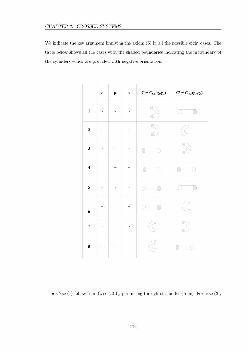
CHAPTER 3. CROSSED SYSTEMS
We indicate the key argument implying the axiom (6) in all the possible eight cases. The
table below shows all the cases with the shaded boundaries indicating the inboundary of
the cylinders which are provided with negative orientation.
ε µ ν C = Cε,µ(g1,g2) C' = C-µ,ν(g3,g4)
1 - - -
2 - - +
3 - + -
4 - + +
5 + - -
6+ - +
7 + + -
8 + + +
• Case (1) follow from Case (3) by permuting the cylinder under gluing. For case (3),
116
CHAPTER 3. CROSSED SYSTEMS
we mainly use axiom (3.1):
τ(C′) ◦ τ(C) = φg−1
4 g−12 g1g2g4
(ϕg−1
2 g1g2,g4⊗ 1)(ϕg1,g
−12⊗ 1)
= φg−14 g−1
2 g1g2g4
(ϕg−1
2 g1g2,g4· ϕg1,g−1
2⊗ 1)
= φg−14 g−1
2 g1g2g4
(ϕg1,g
−14 g−1
2⊗ 1)
= τ(C−−(g1, (g2g4)−1))
• Case (2) We need to prove that:
[τ(C−−(g1, g2))⊗ 1
]◦[1⊗ τ(C++(g3, g4))
]= τ
(C−+(g1, g2g4)
)(3.22)
where g3 = g−12 g−1
1 g2. Observe the obvious X -homeomorphism between the follow-
ing composition(gluing) of (2,X )-annuli:
[C−+(g1, g
−12 )]◦[C−+(g−1
2 g1g2, 1) ∪ C++(g1, g2)]∼=X
[C−+(g1, 1) ∪ C++(g1, g2)
]◦[C−+(g1, g
−12 ) ∪ C−+(g1, 1) ∪ C−+(g−1
2 g−11 g2, 1)
].
which algebraically can be interpreted as:
(ϕg1,g
−12⊗ 1⊗ 1
)(1⊗ Fg3,g4
)=(1⊗ Fg3,g4
)ϕg1,g
−12
Now putting the values(morphisms) for the left side of equation (3.22), we get :
(φg−1
2 g1g2⊗ 1)(ϕg1,g
−12⊗ 1⊗ 1
)(1⊗ Fg3,g4
)=
(φg−1
2 g1g2⊗ 1)(
1⊗ Fg3,g4)ϕg1,g
−12
= ϕg−13 ,g−1
4ϕg1,g
−12
= ϕg1,(g2g4)−1
= τ(C−+(g1, g2g4)
).
117
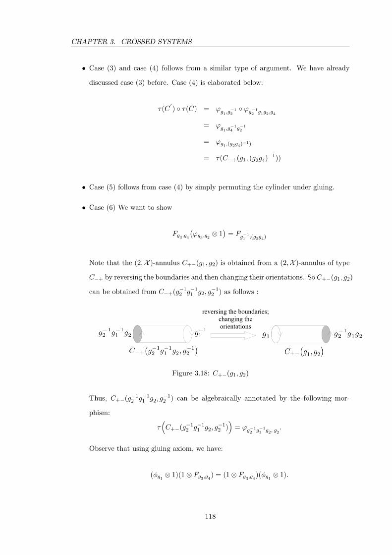
CHAPTER 3. CROSSED SYSTEMS
• Case (3) and case (4) follows from a similar type of argument. We have already
discussed case (3) before. Case (4) is elaborated below:
τ(C′) ◦ τ(C) = ϕg1,g
−12◦ ϕg−1
2 g1g2,g4
= ϕg1,g−14 g−1
2
= ϕg1,(g2g4)−1)
= τ(C−+(g1, (g2g4)−1))
• Case (5) follows from case (4) by simply permuting the cylinder under gluing.
• Case (6) We want to show
Fg3,g4(ϕg3,g2 ⊗ 1
)= Fg−1
1 ,(g2g4)
Note that the (2,X )-annulus C+−(g1, g2) is obtained from a (2,X )-annulus of type
C−+ by reversing the boundaries and then changing their orientations. So C+−(g1, g2)
can be obtained from C−+(g−12 g−1
1 g2, g−12 ) as follows :
reversing the boundaries; changing the orientations
Figure 3.18: C+−(g1, g2)
Thus, C+−(g−12 g−1
1 g2, g−12 ) can be algebraically annotated by the following mor-
phism:
τ(C+−(g−1
2 g−11 g2, g
−12 ))
= ϕg−12 g−1
1 g2, g2.
Observe that using gluing axiom, we have:
(φg1 ⊗ 1)(1⊗ Fg3,g4) = (1⊗ Fg3,g4)(φg1 ⊗ 1).
118
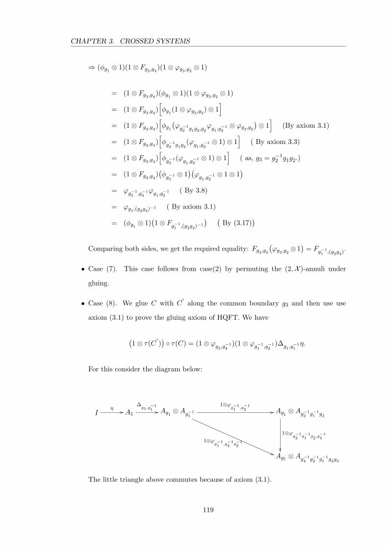
CHAPTER 3. CROSSED SYSTEMS
⇒ (φg1 ⊗ 1)(1⊗ Fg3,g4)(1⊗ ϕg3,g2 ⊗ 1)
= (1⊗ Fg3,g4)(φg1 ⊗ 1)(1⊗ ϕg3,g2 ⊗ 1)
= (1⊗ Fg3,g4)[φg1(1⊗ ϕg3,g2)⊗ 1
]= (1⊗ Fg3,g4)
[φg1(ϕg−1
2 g1g2,g2ϕg1,g
−12⊗ ϕg3,g2
)⊗ 1]
(By axiom 3.1)
= (1⊗ Fg3,g4)[φg−1
2 g1g2(ϕg1,g
−12⊗ 1)⊗ 1
]( By axiom 3.3)
= (1⊗ Fg3,g4)[φg−1
3(ϕg1,g
−12⊗ 1)⊗ 1
]( as, g3 = g−1
2 g1g2.)
= (1⊗ Fg3,g4)(φg−1
3⊗ 1)(ϕg1,g
−12⊗ 1⊗ 1
)= ϕg−1
3 ,g−14ϕg1,g
−12
( By 3.8)
= ϕg1,(g2g4)−1 ( By axiom 3.1)
= (φg1 ⊗ 1)(1⊗ Fg−1
1 ,(g2g4)−1
) (By (3.17)
)Comparing both sides, we get the required equality: Fg3,g4
(ϕg3,g2 ⊗ 1
)= Fg−1
1 ,(g2g4).
• Case (7). This case follows from case(2) by permuting the (2,X )-annuli under
gluing.
• Case (8). We glue C with C′
along the common boundary g3 and then use use
axiom (3.1) to prove the gluing axiom of HQFT. We have
(1⊗ τ(C
′))◦ τ(C) = (1⊗ ϕg3,g−1
4)(1⊗ ϕg−1
1 ,g−12
)∆g1,g−11η.
For this consider the diagram below:
Iη // A1
∆g1,g−11 // Ag1 ⊗Ag−1
1
1⊗ϕg−11 ,g−1
4 g−12
((QQQQQQQQQQQQQQQQQQQQQQQQQQQQ
1⊗ϕg−11 ,g−1
2 // Ag1 ⊗Ag−12 g−1
1 g2
1⊗ϕg−12 g−1
1 g2,g−14
��Ag1 ⊗Ag−1
4 g−12 g−1
1 g2g4
The little triangle above commutes because of axiom (3.1).
119
CHAPTER 3. CROSSED SYSTEMS
Next we check the gluing condition when a (2,X )-annuli Cε0,ε1 is composed with a
(2,X )-pant Pε,µ,ν . By the topological invariance of τ , it is enough to consider the gluing
performed along an X -homeomorphism: C0ε0
= Nν so that ε0 = −ν. We have 16 cases
corresponding to different signs ε1, ε, µ, ν. The table below shows all the cases; the shaded
boundaries are with the negative orientation which shall indicate the inboundary of the
pants/cylinders.
120
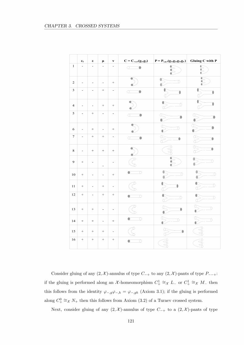
CHAPTER 3. CROSSED SYSTEMS
ε1 ε µ ν C = C-ν,ε1(g1,g2) P = Pε,µ,ν(g1,g2,g3,g4 ) Gluing C with P1 - - - -
2 - - - +
3 - - + -
4 - - + +
5 - + - -
6 - + - +
7 - + + -
8 - + + +
9 + --
-
10 + - - +
11 + - + -
12 + - + +
13 + + - -
14 + + - +
15 + + + -
16 + + + +
Consider gluing of any (2,X )-annulus of type C−+ to any (2,X )-pants of type P−−+:
if the gluing is performed along an X -homeomorphism C1+∼=X L− or C1
+∼=X M− then
this follows from the identity ϕ−,gϕ−,h = ϕ−,gh (Axiom 3.1); if the gluing is performed
along C0+∼=X N+ then this follows from Axiom (3.2) of a Turaev crossed system.
Next, consider gluing of any (2,X )-annulus of type C−+ to a (2,X )-pants of type
121
CHAPTER 3. CROSSED SYSTEMS
P−−−. The gluing axiom holds for such a composition(such a gluing produces again
P−−−). If the gluing is performed along L or M then this follows from the identity . The
existence of a self-X -homeomorphism of P−−− mapping N onto L shows that the claim
holds also for the gluing along N .
The cases where ε0 = −ν and the triple ε, µ, ν contains at least two minuses follows
the arguments discussed above. The cases where ε = µ are checked one by one using
directly the definitions and the properties of τ established above, specifically, the gluing
axiom for the (2,X )-annuli discussed above. The key argument in all these cases is that
the tensor contractions along different tensor factors commute. The case ε = −, µ = +
reduces to ε = +, and µ = − by the topological invariance. Assume that ε = +, µ = −. If
ν = +, ε1 = + then the gluing axiom follows again from definitions. The remaining three
cases (µ = +, ε1 = −), and (ν = −, ε1 = ±) can be deduced using the multiplicativity of
τ , which we have discussed just before the lemma.
The gluing axiom for an HQFT holds for a composition of any cylinder of type C−+ to
P−−+: if the gluing is performed along an X -homeomorphism ∂1C+ = L− or ∂1C+ = M−
then this follows from the axiom(3.1); if the gluing is performed along ∂0C− = N+ then
this follows from axiom (3.2). A cylinder of type C−+ when glued to P−−− produces
again P−−−. If the gluing is performed along L or M then this follows from the axiom
(3.1). The existence of a self-homeomorphism of P−−− mapping N onto M shows that
the claim holds also for the gluing along N .
Now, consider the gluing of an X -disc D+ to an (2,X )-annulus C−+. the gluing axiom
follows from the equality ϕ1,g ◦ η = η for all g ∈ G. Gluing axiom for a composition of
D+ to an (2,X )-pants P−−− follows from the equalities µ1,g(η ⊗ 1g) = µg,1(1g ⊗ η) for
any g ∈ G. This and the definition of τ for (2,X )-pants of types P−−− or P−++ imply
the axiom for any gluing of D+ to such pants. The gluing axiom for a composition of D−
to X -surfaces with≤ 2 holes follows from the already established properties of the gluing
of C−−(1, 1) and D+.
Now consider any connected X -surface W . To compute τ(W ) we need to compute it
on a splitting system of loops. Turaev [Tur99] has argued that τ(W ) neither depends on
the choice of orientations and base points on α1, · · · , αN nor on the choice of a splitting
122
CHAPTER 3. CROSSED SYSTEMS
system of loops on W . His crucial argument is provided by the fact (see [HT80]) that
any two splitting systems of loops on W are related by the following transformations:
(i) isotopy in W ; (ii) adding to a splitting system of loops α1, · · · , αN a simple loop
α ⊂W ∪iαi; (iii) deleting a loop from a splitting system of loops, provided the remaining
loops form a splitting system; (iv) replacing one of the loops αi of a splitting system
adjacent to two different pants P1, P2 by a simple loop lying in IntP1∪ IntP1∪αi, meeting
αi transversally in two points and splitting both P1 and P2 into annuli; (v) replacing one
of the loops of a splitting system by a simple loop meeting it transversally in one point
and disjoint from the other loops. He has checked the invariance of τ(W ) under these
transformations. 2
Theorem 3.5.3 A Turaev G-crossed system (Ag, µ,∆, ε) in S defines (up to isomor-
phism) a (1+1)-dimensional symmetric HQFT over K(G, 1) space with values in S.
Proof: We have realised Turaev G-crossed system (Ag, µ,∆, ε) as the underlying system
of (1+1)-dimensional X -HQFT (Z, τ) with X = K(G; 1) using the Lemma (3.5.1) and
Lemma (3.5.2).
2
Suppose X is an Eilenberg-MacLane space with X = K(G; 1) for a group G. Let us
recall from Section (3.4.2) the category T (G,S) of Turaev crossed G-systems in S and
from Section (3.3) the category Z2(X , S) of (1+1)-dimensional X -HQFTs with values in
S. We wish to establish a functor from the category Z2(X ) to T (G,S). The functor
is clear on objects. It simply takes any X -HQFT to its underlying Turaev G-crossed
system A = {Ag} [Theorem (3.4.6)]. Let ρ = {ρM : AM → A′M} be a morphism between
X -HQFTs (Z, τ) and (Z′, τ′). Suppose A = {Ag} and A
′= {A′h} are their respective
underlying Turaev G-crossed systems in S. The morphism ρ in Z2(X ) corresponds to a
morphism between A and A′
in T (G,S). Note that ρ yields a collection {ρf : Af → A′f}
of morphisms in S for the connected 1-dimensional X -manifolds. The commutativity
of the natural square diagrams associated with the X -cobordisms P−−+(f, g, 1, 1), D+,
C−−(f, 1), and C−+(f, g−1) together with the fact that ρ∅ = idIC in Z2(X ) imply that
the collection {ρf : Af → A′f} of morphisms in S commutes with the multiplication, and
the action of G; and preserves the unit and the inner product(form). This establishes a
123
CHAPTER 3. CROSSED SYSTEMS
functor
F : Z2(X , S)→ T (G,S).
Proposition 3.5.4 Given a monoidal category S, if X = (X,x) is a K(G; 1) space, then
the functor F : Z2(X , S)→ T (G,S) is an equivalence of categories.
Proof: The surjectivity for objects in T (G,S) has been established in Theorem (3.5.3).
Let us now establish that for any two (1+1)-dimensional X -HQFTs (Z, τ) and (Z′, τ′) with
values in S and with the underlying Turaev G-crossed systems A, A′, the homomorphism
Hom(
(Z, τ), (Z′, τ′))→ Hom(A,A
′) (3.23)
is bijective. The injectivity of the morphism in (3.23) is obvious since all 1-dimensional X -
manifolds are disjoint unions of loops and therefore any two morphisms (Z, τ)→ (Z′, τ′)
coinciding on loops coincide on all 1-dimensional X -manifolds.
Now to establish the surjectivity of the morphism in (3.23) note that every morphism
of a G-crossed system ρ : A → A′
defines a morphism ZM → Z′M for any connected
1-dimensional X -manifold M. These morphisms extend to non-connected X -manifolds
M by multiplicativity. We need to show that the resulting family of morphisms {ρM :
ZM → A′}M would make the natural square diagrams related to X -homeomorphisms and
X -surfaces commutative. The part concerning the X -homeomorphisms is obvious. As ex-
plained before, every X -surface can be obtained by gluing from a finite collection of the ba-
sic X -surfaces of type D+, C−+(f, g), C−−(f, 1), C++(f, g), and P−−+(f, g, 1, 1). There-
fore it suffices to check the commutativity of the square diagrams associated with these
X -surfaces. For D+ and P−−+(f, g, 1, 1) this follows from the assumption that ρ com-
mutes with multiplication and preserves the unit. For C−+(f, g), C−−(f, 1), C++(f, g),
this follows from the formula’s (3.15) - (3.17) and the assumption that ρ preserves the in-
ner product and commutes with the action of G. Thus the morphism in (3.23) is bijective.
This completes the proof. 2
124
CHAPTER 3. CROSSED SYSTEMS
3.6 Examples
The goal of this section is to construct examples of a Turaev crossed system which we
defined in the Section 3.4. We start with a commutative ring K with a unit. Let π and
H be groups such that π acts on H. Let θ be a normalised 2-cochain of H with values in
K×.
Here is a briefing of what we do in this section. In the first subsection we construct
a Turaev crossed π-system in the category of K-modules starting from a crossed module
(H,π, t, ϕ). In the second subsection we define a twisted category Aσ,τπ where (σ, τ) is an
abelian 3-cocycle for a group π with values in K× and discuss some properties of such
categories in general. In the last subsection we work out another set of examples for a
Turaev crossed π-system taking values in the twisted category Aσ,τπ .
3.6.1 Crossed module
Given that H and π are multiplicative groups, let (H,π, t, u) forms a crossed mod-
ule where t is a group homomorphism from H to π and π acts on H via u. Let
θ = {θ(f, g) ∈ K×}f,g∈H be a normalised 2-cocycle of H. For any α ∈ T := Im t,
define Lα =⊕
t(h)=αKh. Then each Lα is a K-module. Let us denote the collection of
these K-modules as
L := {Lα|α ∈ T}.
We aim to provide L with a structure of a Turaev T -crossed system. For h, g in H such
that t(h) = α and t(g) = β for some α, β ∈ T , consider the following equations:
h⊗ g 7→ θ(h, g)hg,
k 7→ k.1H .
Extending these maps equips L with multiplications µα,β : Lα ⊗ Lβ → Lαβ and a unit
η : K → L1 which are all K-module morphisms. Let us define a map on H ×H taking
values in K× as:
(f, g) 7→ θ(f, g) (3.24)
125
CHAPTER 3. CROSSED SYSTEMS
if fg = 1 and zero otherwise. For any pair f, g ∈ H such that fg = 1, t(f) = α and
t(g) = β, for some α, β ∈ T , the map given by (3.24) can be extended to a K-module
morphism φ : Lα ⊗ Lβ → K which gives a pairing on L.
Let us define a map onH×H taking values inK× given as< f, g >= θ(f, g)θ(fgf−1, f)−1.
We use this map to define a crossing on L. Let us call Mor(L) to be the set of all mor-
phisms of K-modules between different components of L. Explicitly, it is given as:
Mor(L) =⋃α∈T
(uβ∈T Hom(Lβ, Lαβα−1)
).
Then any element in Mor(L) is a collection of morphisms between different components
of L.
Let us define a map ϕ : H → Mor(L) by extending the map given below. For f ∈ H,
such that t(f) = α, the β-component of ϕf ,(ϕf)β
:= ϕ(f)β : Lβ → Lαβα−1 is defined by
extending
ϕf (g) =< f, g > fgf−1 (3.25)
for g ∈ H such that β = t(g). For any f ∈ H, we say ϕf = I if ϕf is identity on every
component, that is, ϕf : Lg → Lfgf−1 is identity for all f ∈ G provided gfg−1 = f .
Let us now define a crossing ϕ : T → Mor(L) for the system L as the extension of ϕ
onto T .
Consider the following diagram: H
t
��
ϕ // Mor(L)
T
ϕ
::
For ϕ to be well defined it suffices to show that ϕt|Z = ϕ|Z = Id where Z = Ker t.
Thus we have the following proposition:
Proposition 3.6.1 Given g ∈ H, if for all z ∈ Ker t
θ(g, z) = θ(z, g), (3.26)
then the crossing ϕ : T → Mor(L) becomes a well defined map.
Proof: Note that Z is central in H. Suppose ϕ|Z = Id, then equation (3.25) restricted
126
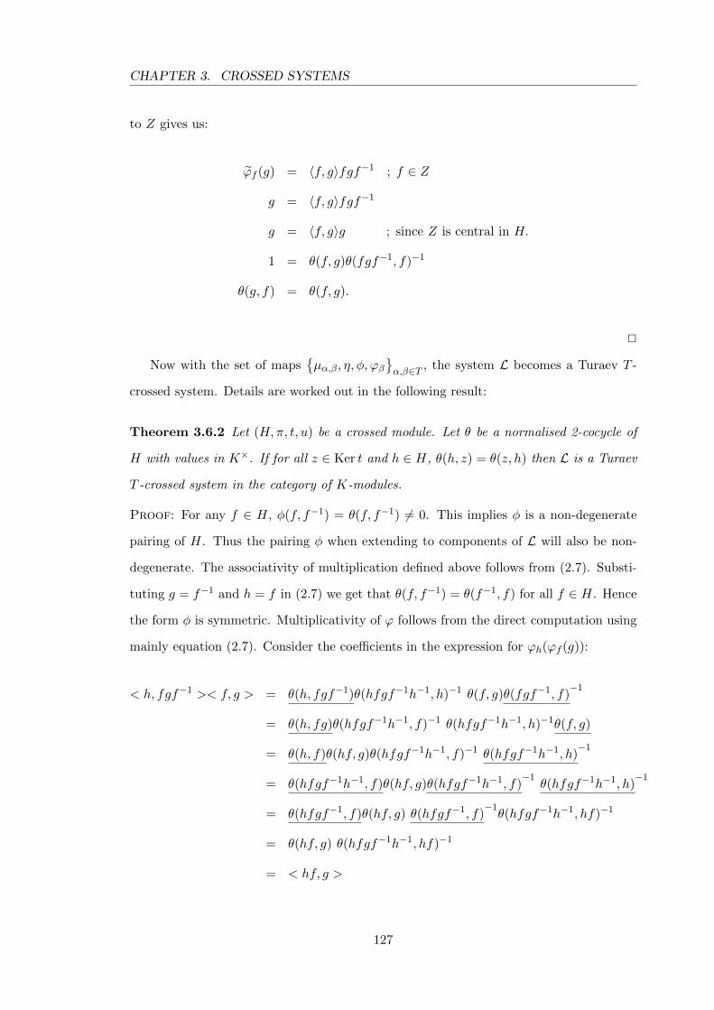
CHAPTER 3. CROSSED SYSTEMS
to Z gives us:
ϕf (g) = 〈f, g〉fgf−1 ; f ∈ Z
g = 〈f, g〉fgf−1
g = 〈f, g〉g ; since Z is central in H.
1 = θ(f, g)θ(fgf−1, f)−1
θ(g, f) = θ(f, g).
2
Now with the set of maps{µα,β, η, φ, ϕβ
}α,β∈T , the system L becomes a Turaev T -
crossed system. Details are worked out in the following result:
Theorem 3.6.2 Let (H,π, t, u) be a crossed module. Let θ be a normalised 2-cocycle of
H with values in K×. If for all z ∈ Ker t and h ∈ H, θ(h, z) = θ(z, h) then L is a Turaev
T -crossed system in the category of K-modules.
Proof: For any f ∈ H, φ(f, f−1) = θ(f, f−1) 6= 0. This implies φ is a non-degenerate
pairing of H. Thus the pairing φ when extending to components of L will also be non-
degenerate. The associativity of multiplication defined above follows from (2.7). Substi-
tuting g = f−1 and h = f in (2.7) we get that θ(f, f−1) = θ(f−1, f) for all f ∈ H. Hence
the form φ is symmetric. Multiplicativity of ϕ follows from the direct computation using
mainly equation (2.7). Consider the coefficients in the expression for ϕh(ϕf (g)):
< h, fgf−1 >< f, g > = θ(h, fgf−1)θ(hfgf−1h−1, h)−1 θ(f, g)θ(fgf−1, f)−1
= θ(h, fg)θ(hfgf−1h−1, f)−1 θ(hfgf−1h−1, h)−1θ(f, g)
= θ(h, f)θ(hf, g)θ(hfgf−1h−1, f)−1 θ(hfgf−1h−1, h)−1
= θ(hfgf−1h−1, f)θ(hf, g)θ(hfgf−1h−1, f)−1
θ(hfgf−1h−1, h)−1
= θ(hfgf−1, f)θ(hf, g) θ(hfgf−1, f)−1θ(hfgf−1h−1, hf)−1
= θ(hf, g) θ(hfgf−1h−1, hf)−1
= < hf, g >
127
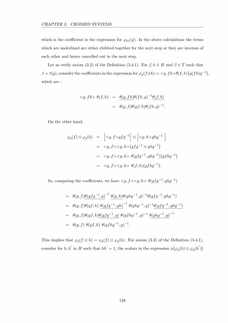
CHAPTER 3. CROSSED SYSTEMS
which is the coefficient in the expression for ϕhf (g). In the above calculations the terms
which are underlined are either clubbed together for the next step or they are inverses of
each other and hence cancelled out in the next step.
Let us verify axiom (3.2) of the Definition (3.4.1). For f, h ∈ H and β ∈ T such that
β = t(g), consider the coefficients in the expression for ϕg(f⊗h) = <g, fh>θ(f, h)(g(fh)g−1
),
which are :
<g, fh> θ(f, h) = θ(g, fh)θ(fh, g)−1θ(f, h)
= θ(g, f)θ(gf, h)θ(fh, g)−1.
On the other hand,
ϕg(f)⊗ ϕg(h) =[<g, f>gfg−1
]⊗[<g, h>ghg−1
]= <g, f><g, h>
(gfg−1 ⊗ ghg−1
)= <g, f><g, h> θ(gfg−1, ghg−1)
(gfhg−1
)= <g, f><g, h> θ(f, h)
(gfhg−1
).
So, comparing the coefficients, we have <g, f><g, h> θ(gfg−1, ghg−1)
= θ(g, f)θ(gfg−1, g)−1
θ(g, h)θ(ghg−1, g)−1θ(gfg−1, ghg−1)
= θ(g, f)θ(gf, h) θ(gfg−1, gh)−1
θ(ghg−1, g)−1θ(gfg−1, ghg−1)
= θ(g, f)θ(gf, h)θ(gfg−1, g) θ(gfhg−1, g)−1 θ(ghg−1, g)−1
= θ(g, f) θ(gf, h) θ(gfhg−1, g)−1.
This implies that ϕg(f ⊗ h) = ϕg(f) ⊗ ϕg(h). For axiom (3.3) of the Definition (3.4.1),
consider for h, h′
in H such that hh′
= 1, the scalars in the expression φ(ϕg(h)⊗ϕg(h
′))
128
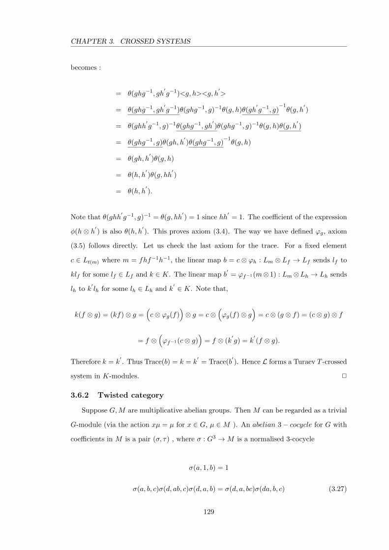
CHAPTER 3. CROSSED SYSTEMS
becomes :
= θ(ghg−1, gh′g−1)<g, h><g, h
′>
= θ(ghg−1, gh′g−1)θ(ghg−1, g)−1θ(g, h)θ(gh
′g−1, g)
−1θ(g, h
′)
= θ(ghh′g−1, g)−1θ(ghg−1, gh
′)θ(ghg−1, g)−1θ(g, h)θ(g, h
′)
= θ(ghg−1, g)θ(gh, h′)θ(ghg−1, g)
−1θ(g, h)
= θ(gh, h′)θ(g, h)
= θ(h, h′)θ(g, hh
′)
= θ(h, h′).
Note that θ(ghh′g−1, g)−1 = θ(g, hh
′) = 1 since hh
′= 1. The coefficient of the expression
φ(h ⊗ h′) is also θ(h, h′). This proves axiom (3.4). The way we have defined ϕg, axiom
(3.5) follows directly. Let us check the last axiom for the trace. For a fixed element
c ∈ Lt(m) where m = fhf−1h−1, the linear map b = c ⊗ ϕh : Lm ⊗ Lf → Lf sends lf to
klf for some lf ∈ Lf and k ∈ K. The linear map b′
= ϕf−1(m⊗ 1) : Lm⊗Lh → Lh sends
lh to k′lh for some lh ∈ Lh and k
′ ∈ K. Note that,
k(f ⊗ g) = (kf)⊗ g =(c⊗ ϕg(f)
)⊗ g = c⊗
(ϕg(f)⊗ g
)= c⊗ (g ⊗ f) = (c⊗ g)⊗ f
= f ⊗(ϕf−1(c⊗ g)
)= f ⊗ (k
′g) = k
′(f ⊗ g).
Therefore k = k′. Thus Trace(b) = k = k
′= Trace(b
′). Hence L forms a Turaev T -crossed
system in K-modules. 2
3.6.2 Twisted category
Suppose G,M are multiplicative abelian groups. Then M can be regarded as a trivial
G-module (via the action xµ = µ for x ∈ G, µ ∈M ). An abelian 3− cocycle for G with
coefficients in M is a pair (σ, τ) , where σ : G3 →M is a normalised 3-cocycle
σ(a, 1, b) = 1
σ(a, b, c)σ(d, ab, c)σ(d, a, b) = σ(d, a, bc)σ(da, b, c) (3.27)
129
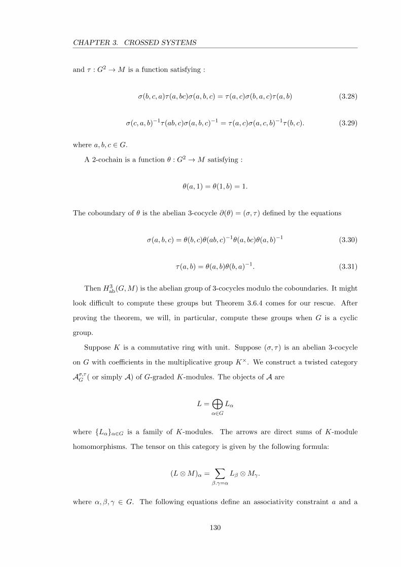
CHAPTER 3. CROSSED SYSTEMS
and τ : G2 →M is a function satisfying :
σ(b, c, a)τ(a, bc)σ(a, b, c) = τ(a, c)σ(b, a, c)τ(a, b) (3.28)
σ(c, a, b)−1τ(ab, c)σ(a, b, c)−1 = τ(a, c)σ(a, c, b)−1τ(b, c). (3.29)
where a, b, c ∈ G.
A 2-cochain is a function θ : G2 →M satisfying :
θ(a, 1) = θ(1, b) = 1.
The coboundary of θ is the abelian 3-cocycle ∂(θ) = (σ, τ) defined by the equations
σ(a, b, c) = θ(b, c)θ(ab, c)−1θ(a, bc)θ(a, b)−1 (3.30)
τ(a, b) = θ(a, b)θ(b, a)−1. (3.31)
Then H3ab(G,M) is the abelian group of 3-cocycles modulo the coboundaries. It might
look difficult to compute these groups but Theorem 3.6.4 comes for our rescue. After
proving the theorem, we will, in particular, compute these groups when G is a cyclic
group.
Suppose K is a commutative ring with unit. Suppose (σ, τ) is an abelian 3-cocycle
on G with coefficients in the multiplicative group K×. We construct a twisted category
Aσ,τG ( or simply A) of G-graded K-modules. The objects of A are
L =⊕α∈G
Lα
where {Lα}α∈G is a family of K-modules. The arrows are direct sums of K-module
homomorphisms. The tensor on this category is given by the following formula:
(L⊗M)α =∑β.γ=α
Lβ ⊗Mγ .
where α, β, γ ∈ G. The following equations define an associativity constraint a and a
130
CHAPTER 3. CROSSED SYSTEMS
braiding c in A
a((x⊗ y)⊗ z) = σ(α, β, γ)(x⊗ (y ⊗ z))
c(x⊗ y) = τ(α, β)y ⊗ x
where x ∈ Lα, y ∈Mβ, z ∈ Nγ . We then extend the definition by linearity to define it on
the objects of the category. In this way, A becomes a monoidal category of G-graded K-
modules. In other words, A is a monoidal category of KG-comodules with associativity
given by σ.
Proposition 3.6.3 Let (σ, τ) and (σ′, τ′) be any two representatives of their equivalence
classes. If [σ, τ ] = [σ′, τ′] ∈ H3
ab(G,K×), then we get a braided tensor isomorphism
between the categories Aσ,τG and Aσ′,τ′
G .
Proof: Consider the identity functor I from the category Aσ,τG to the category Aσ′,τ′
G .
We claim that it is in fact a braided tensor isomorphism. Let k : G2 → M be a function
satisfying k(a, 1) = k(1, b) = 1, such that
(σ, τ)(σ′, τ ′)−1 = ∂(k).
Define tensor isomorphism via the natural transformation φL,M : I(L)⊗I(M)→ I(L⊗M)
as φL,M (∑lβ ⊗mγ) =
∑k(β, γ)(lβ ⊗mγ), where lβ ∈ Lβ and mγ ∈Mγ for α, β ∈ π. Let
us first show that φ is a tensor functor. Given any three objects M,N,L in the category
Aσ,τG , we want the the following condition is satisfied
a · (φM⊗N,L) · (φM,N ⊗ 1L) = φM,(N⊗L) · (1M ⊗ φN,L) · a′ .
For any b, c, e ∈ G , when a typical element∑
(mb⊗nc)⊗ le is applied to the equation
131
CHAPTER 3. CROSSED SYSTEMS
above, the left hand side becomes :
= a · (φM⊗N,L) · (φM,N ⊗ 1L)(∑
(mb ⊗ nc)⊗ le)
= a · (φM⊗N,L)(∑
φM,N (mb ⊗ nc)⊗ le))
= a · (φM⊗N,L)(∑
k(b, c)(mb ⊗ nc)⊗ le)
= a(∑
k(bc, e)(∑
k(b, c)(mb ⊗ nc)⊗ le)
=∑
σ(b, c, e) k(bc, e) k(b, c)(mb ⊗ (nc ⊗ le))
and after applying∑
(mb ⊗ nc) ⊗ le to the equation above, the right hand side of the
equation becomes :
= φM,N⊗L · (1M ⊗ φN,L) · a′(∑
(mb ⊗ nc)⊗ le)
= φM,N⊗L · (1M ⊗ φN,L)(∑
σ′(b, c, e)mb ⊗ (nc ⊗ le))
= φM,N⊗L(∑
σ′(b, c, e)mb ⊗ φN,L(nc ⊗ le))
= φM,N⊗L(∑
σ′(b, c, e) k(c, e)mb ⊗ (nc ⊗ le))
=∑
σ′(b, c, e) k(b, ce) k(c, e)(mb ⊗ (nc ⊗ le))
The coefficients of the left side σ(b, c, e) k(bc, e) k(b, c) equals the coefficients on the
right side σ′(b, c, e) k(b, ce) k(c, e) using (3.15) and (σ, τ)(σ
′, τ ′)−1 = ∂(k). To show that
the isomorphism is also braided we need to show the following
φN,M · c′M,N = cM,N · φM,N
For any b, c ∈ G and using the equation τ(b, c) = k(b, c)k−1(c, b) one can show that
the isomorphism is also braided. Applying a general element∑mb ⊗ nc, the left hand
side of the equation above becomes :
= φM,N · c′M,N (
∑mb ⊗ nc)
= φM,N (∑
τ′(b, c)nc ⊗mb)
=∑
τ′(b, c)k(c, b)nc ⊗mb
132
CHAPTER 3. CROSSED SYSTEMS
Applying∑mb ⊗ nc, the right hand side of the equation above becomes :
= cM,N · φM,N (∑
mb ⊗ nc)
= cM,N (∑
k(b, c)mb ⊗ nc
=∑
τ(b, c)k(b, c)nc ⊗mb
The coefficient of left side τ′(b, c) k(c, b) equals the coefficient on right side τ(b, c) k(b, c)
using (3.16) and (σ, τ)(σ′, τ ′)−1 = ∂(k). This completes the proof.
2
We recall the definition of a quadratic function. A function q : G → M between two
abelian groups G,M is called quadratic when q(xy)q(x)−1q(y)−1 is a bilinear function of
x, y. This amounts to the following two conditions:
(i) q(xyz) q(xy)−1q(yz)−1q(zx)−1q(x) q(y) q(z) = 1,
(ii) q(x) = q(x−1).
Now to any abelian 3-cocycle (σ, τ) we assign the function q(x) = τ(x, x) ∈ M as
its trace. By (3.21), the trace of a coboundary is identity, and one can show that the
trace satisfies the above two identities. Thus traces are quadratic functions. We have the
following result which appears in several papers without a proof. We discuss its proof
here:
Theorem 3.6.4 ([Mac52], [Eil52], [EM53]) The function assigning to each abelian 3-
cocycle its trace induces an isomorphism of H3ab(G,M) to the group of all quadratic func-
tions on G to M .
Proof: For a fixed M , trace is natural in abelian groups G. Note that every abelian
group is a filtered colimit of finitely generated abelian groups. Moreover, every finitely
generated abelian group is a finite direct sum of cyclic groups. So it suffices to verify the
isomorphism when G is cyclic as quadratic functions into M preserve filtered colimits.
Surjectivity: Suppose q : G → M is a quadratic function. Put ν = q(1). Define
τ(x, y) = νxy. If G is infinite, (1, τ) is an abelian 3-cocycle whose trace is q. If G has
order n, notice that ν2n = νn2
= 1 in order for q to be well defined. Let σ be the 3-cocycle
133
CHAPTER 3. CROSSED SYSTEMS
defined with trace q. The standard form for such a σ is (cf. Chapter-2, Section 2.3)
σ(x, y, z) =
1 for y + z < n
νxn for y + z ≥ n(3.32)
Then (σ, τ) is an abelian 3-cocycle.
Injectivity: It is done in the following two cases.
Case 1 : G = Z. Let (σ, τ) be an abelian 3-cocycle such that τ(x, x) = 1. Since
H3(G,M) = 1, we have σ = dθ for some 2-cochain θ. Let
(σ′, τ′) = (σ, τ)∂θ−1 = (1, τ
′).
Then τ′(x, y) = τ(x, y)θ(x, y)−1θ(y, x). Substituting σ
′= 1 in (3.28) and (3.29), we
get
τ′(x, yz) = τ
′(x, z)τ
′(x, y),
τ′(xy, z) = τ
′(x, z)τ
′(y, z).
Equating for τ′(x, z) in the above two equations, we get
τ′(xy, z)τ
′(y, z) = τ
′(xy, z)τ
′(x, y).
Substitute x = 1, z = y−1 in the above equation, we get
τ′(1, 1)τ
′(y, y−1) = τ
′(y, y−1)τ
′(1, y).
Thus, τ′(1, y) = 1. Similarly we can show τ
′(y, 1) = 1. Then using (3.28) and (3.29)
and that σ′
= 1, τ′(x, y) = 1 follows by induction.
Case 2 : G = Zn. Let (σ, τ) be an abelian 3-cocycle such that τ(x, x) = 1. Choose
a 2-cochain θ such that (σ′, τ′) = (σ, τ)∂θ−1 and σ
′is standard for some ν, as in
(3.32). Similar to the Case (1), we have τ′(x, x) = 1. Substitute b = 1 in (3.29).
We get
σ′(1, c, a) = σ
′(1, a, c)τ
′(a, 1).
134
CHAPTER 3. CROSSED SYSTEMS
Since G is abelian (3.32) implies that σ′(1, c, a) = σ
′(1, a, c). Thus, from the above
equation, τ′(a, 1) = 1. Similarly we can show τ
′(1, a) = 1. Then using again (3.28)
and (3.29) and the standard form of σ′, one deduces by induction that τ
′(x, y) = 1.
Then the standard form for σ′
reduces to 1. This proves injectivity.
2
We are now in a better position to calculate H3ab(G,M) using the above theorem. In
the case when G is an infinite cyclic group Z, let q : G → M be a quadratic function.
Then it is simply a group homomorphism. Indeed the group of all quadratic functions on
Z to any abelian group M is M itself, thus H3ab(Z,M) = M . In the case when G = Zn
is a cyclic group of order n, let q : Zn → M be a quadratic function on G. Then it is
simply a group homomorphism such that q(1)2n = q(1)n2
= 1 for q to be a well defined
quadratic function. Thus the group of all quadratic functions on Z/n to M is isomorphic
to Hom(Z/(n2, 2n),M
). Hence,
H3ab(Z/n,M) ∼= Hom
(Z/(n2, 2n),M
).
Consider for example M as C× and n = 6 so that,
H3ab(Z/6,C×) ∼= Hom(Z/(n2, 2n),C×) = Hom(Z/12,C×) ∼= Z/12.
An explicit formula for defining a 3-cocycle can be worked out using the proof of Theorem
(3.6.4). Accordingly, we define a 3-cocycle (h,c) as follows. Let ν = e2πι/12 ∈ C× then
ν62 = ν2×6 = 1. Define,
h(x, y, z) =
1 for yz < n
νxn for yz ≥ n
c(x, y) = νxy.
where x, y, z ∈ Z/n and ν = c(1, 1). One can easily check that (h, c) so defined is an
abelian 3-cocycle.
135
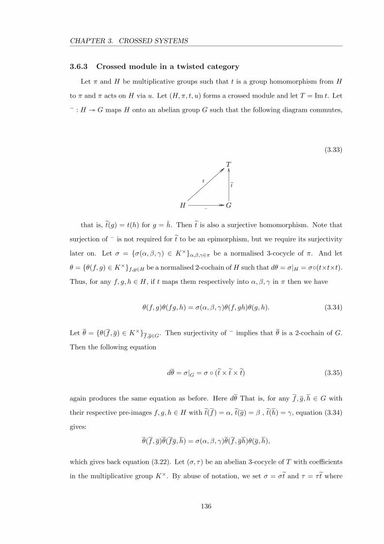
CHAPTER 3. CROSSED SYSTEMS
3.6.3 Crossed module in a twisted category
Let π and H be multiplicative groups such that t is a group homomorphism from H
to π and π acts on H via u. Let (H,π, t, u) forms a crossed module and let T = Im t. Let
− : H � G maps H onto an abelian group G such that the following diagram commutes,
(3.33)
T
H −// //
t
== ==||||||||||||||||G
t
OO
that is, t(g) = t(h) for g = h. Then t is also a surjective homomorphism. Note that
surjection of − is not required for t to be an epimorphism, but we require its surjectivity
later on. Let σ = {σ(α, β, γ) ∈ K×}α,β,γ∈π be a normalised 3-cocycle of π. And let
θ = {θ(f, g) ∈ K×}f,g∈H be a normalised 2-cochain ofH such that dθ = σ|H = σ◦(t×t×t).
Thus, for any f, g, h ∈ H, if t maps them respectively into α, β, γ in π then we have
θ(f, g)θ(fg, h) = σ(α, β, γ)θ(f, gh)θ(g, h). (3.34)
Let θ = {θ(f, g) ∈ K×}f,g∈G. Then surjectivity of − implies that θ is a 2-cochain of G.
Then the following equation
dθ = σ|G = σ ◦ (t× t× t) (3.35)
again produces the same equation as before. Here dθ That is, for any f, g, h ∈ G with
their respective pre-images f, g, h ∈ H with t(f) = α, t(g) = β , t(h) = γ, equation (3.34)
gives:
θ(f, g)θ(fg, h) = σ(α, β, γ)θ(f, gh)θ(g, h),
which gives back equation (3.22). Let (σ, τ) be an abelian 3-cocycle of T with coefficients
in the multiplicative group K×. By abuse of notation, we set σ = σt and τ = τ t where
136
CHAPTER 3. CROSSED SYSTEMS
σ and τ on the right hand side correspond to the pullbacks under t. For α ∈ T , define
Lα =⊕
t(h)=αKh. Then each Lα is an KH-comodule. Note that commutativity of the
above diagram turns each Lα into a KG-comodule where
(Lα)g
=∑
t(h)=α, h=g
Kh =∑t(h)=α
Kh.
Consider the categoryAσ,τG as defined in the last subsection and σ and τ are the restrictions
to G.
Let L = {Lα : α ∈ T} be the collection of KG-comodules. Our goal is to provide this
system with a structure of Turaev T -crossed system in Aσ,τG ,
The multiplications of L can be obtained by extending the map G×G → KG given
by :
(f, g) 7→ θ(f, g)fg. (3.36)
Observe that since G is abelian, we have :
Lαβ = Lt(g)t(h) = Lt(gh) = Lt(hg) = Lβα, (3.37)
for α, β ∈ T such that t(g) = α and t(h) = β.
Note that L1 =⊕
t(h)=1Kh =⊕
h∈Ker (t)Kh. Thus the unit element e of G is also in
L1 which gives the identity of L.
We define a pairing φ on L in a similar way as done in section (3.6.1) which will be
non-degenerate as well as symmetric as before.
We define the dual L∗α of Lα as Lα−1 . Then L∗α =⊕
α−1=t(h)Kh. Let L∗ = {L∗α :
α ∈ T}. The multiplications for the system L∗ is given by the same rule (3.23) as for L.
The unit for L∗ is also the same as for L since L∗1 = L1. For each α ∈ T , Lα ∼= L∗α as
KG-comodules. In fact they are equal to each other as L∗α−1 = Lα. We have the following
result :
Theorem 3.6.5 Let (H,π, t, u) be a crossed module such that − : H � G is a surjective
homomorphism of H onto abelian group G with the diagram (3.23) being commutative.
Let T = Im t. Let θ be a normalised 2-cochain of H and (σ, τ) be an abelian 3-cocycle of
137
CHAPTER 3. CROSSED SYSTEMS
T . If
dθ = σ|H
then the collection L = {Lα|α ∈ T} forms a Frobenius T -graded system in Aσ,τG .
Proof: The multiplication given by the rule (3.36) induces isomorphisms µα,β : (Lα) ⊗
(Lβ)→ Lαβ such that
α ∗ β = θ(α, β) αβ. (3.38)
for α, β ∈ T . These form the multiplications for L. Associativity of these multiplications
is shown below. Let α, β and γ be in T such that their pre images in G are f, g and h
respectively. Then consider,
(α ∗ β) ∗ γ = θ(f, g)((αβ) ∗ γ)
= θ(f, g)θ(fg, h)(αβ)γ
= σ(α, β, γ)θ(g, h)θ(f, gh)(αβ)γ
= σ(α, β, γ)θ(g, h)θ(f, gh)(α(βγ))
= σ(α, β, γ)θ(g, h)(α ∗ (βγ))
= σ(α, β, γ)(α ∗ (β ∗ γ)).
Hence associativity of multiplications for L∗ is also proved. Thus L is a rigid T -algebra in
Aσ,τG . Infact the two systems L and L∗ are isomorphic in Aσ,τG as L-modules. Thus using
Theorem 3.2.8, L is a Frobenius T -graded system in Aσ,τG .
2
Given L to be a Frobenius T -graded system in the category Aσ,τG , we now proceed to
provide it with a structure of a Turaev T -crossed systems in Aσ,τG .
For defining a crossing let us define a map ϕ : G→ Mor(L) by linearly extending the
map given below. For g ∈ G, such that t(g) = β, we set:
ϕ(g)(f) := ϕg(f)⊗ g = τ(α, β)(g ⊗ f) (3.39)
where t(f) = α and ϕg = ϕ(g). We first show that ϕ is a map satisfying the condition
138
CHAPTER 3. CROSSED SYSTEMS
which corresponds to a homomorphism of groups.
Proposition 3.6.6 The map ϕ : G→ Mor(L) satisfies
ϕgh = ϕg ◦ ϕh.
Proof: For any f, g, h ∈ G, consider
ϕgh(f) ∗ gh = τ(f, gh)(gh ∗ f
)= τ(f, gh) θ(g, h)−1
((g ∗ h) ∗ f
)= θ(g, h)−1 τ(f, gh) σ(g, h, f)
(g ∗ (h ∗ f)
)= θ(g, h)−1 τ(f, gh) σ(g, h, f) τ(f, h)−1
(g ∗(ϕh(f) ∗ h
))= θ(g, h)−1 τ(f, gh) τ(f, h)−1 σ(g, h, f) σ(g, hfh−1, h)−1
((g ∗ ϕh(f)
)∗ h)
= X τ(hfh−1, g)−1((ϕgϕh(f) ∗ g
)∗ h)
= Y σ(ghfh−1g−1, g, h)(ϕgϕh(f) ∗
(g ∗ h
))= Z
(ϕgϕh(f) ∗ (gh)
).
where the coefficients X, Y and Z are given as :
X = θ(g, h)−1τ(f, gh)τ(f, h)−1σ(g, h, f)σ(g, hfh−1, h)−1 ;
Y = θ(g, h)−1τ(f, gh)τ(hfh−1, g)τ(f, h)−1σ(g, h, f)σ(g, hfh−1, h)−1 ;
and
Z = τ(f, gh)τ(f, h)−1τ(hfh−1, g)−1σ(g, h, f)σ(g, hfh−1, h)−1σ(ghfh−1g−1, g, h).
We want to show the coefficient Z is identity. Combining the terms τ(f, gh), τ(f, h)−1
and σ(g, h, f) in the expression of Z and using equation (3.28), Z becomes
σ(g, f, h)τ(f, g)τ(hfh−1, g)−1σ(f, g, h)−1σ(g, hfh−1, h)−1σ(ghfh−1g−1, g, h).
139
CHAPTER 3. CROSSED SYSTEMS
Since G is abelian, Z reduces to:
σ(g, f, h)τ(f, g)τ(f, g)−1σ(f, g, h)−1σ(g, f, h)−1σ(f, g, h)
and then every term cancels out so that Z becomes identity.
2
Let us call a morphism ζ ∈ Mor(L) to be an algebra morphism if it respects the
multiplications and the unit of L. We claim each ϕg is an algebra morphism in the
following sense:
Proposition 3.6.7 For each g ∈ G, ϕg ∈ Mor(L) is an algebra morphism.
Proof: It suffices to show that
ϕg(f ⊗ f′) = ϕg(f)⊗ ϕg(f
′)
for f, f′ ∈ G. Consider
ϕg(f ∗ f′) ∗ g = θ(f, f
′)(ϕg(ff
′) ∗ g
)= θ(f, f
′) τ(ff
′, g)(g ∗ ff ′
)= τ(ff
′, g)(g ∗ (f ∗ f ′)
)= σ(g, f, f
′)−1 τ(ff
′, g)(
(g ∗ f) ∗ f ′)
= σ(g, f, f′)−1 τ(ff
′, g) τ(f, g)−1
((ϕg(f) ∗ g
)∗ f ′
)= σ(g, f, f
′)−1 τ(ff
′, g) τ(f, g)−1 σ(gfg−1, g, f
′)(ϕg(f) ∗ (g ∗ f ′)
)= X
(ϕg(f) ∗
(ϕg(f
′) ∗ g
))= Y
((ϕg(f) ∗ ϕg(f
′))∗ g).
where the coefficients X and Y are
X = σ−1(g, f, f′)σ(gfg−1, g, f
′)τ(ff
′, g)τ(f, g)−1τ(f
′, g)−1.
140
CHAPTER 3. CROSSED SYSTEMS
and since G is abelian, we have
Y = σ−1(g, f, f′)σ(gfg−1, g, f
′)σ(gfg−1, gf
′g−1, g)−1τ(ff
′, g)τ(f, g)−1τ(f
′, g)−1
= σ−1(g, f, f′)σ(f, g, f
′)σ(f, f
′, g)−1τ(ff
′, g)τ(f, g)−1τ(f
′, g)−1
= 1 using equation (3.29).
This completes the proof. 2
Let us now define the crossing ϕ : T → Mor(L) for the system L. Consider the
following diagram: G
t
��
ϕ // Mor(L)
T
ϕ
::
For ϕ to be well defined it suffices to show that ϕt|Z = ϕ|Z = Id where Z = {g ∈
G∣∣ ϕg = I}. Thus we have the following proposition:
Proposition 3.6.8 Given that (∂θ)2 = τ |Z , the crossing ϕ : T → Mor(L) becomes a well
defined map.
Proof: Consider g ∈ Z ⊆ G such that t(g) = β. Since g ∈ Z, ϕg = 1g. Then for any
f ∈ G with t(f) = α, equation (3.39) becomes f ⊗ h = τ(α, β) h⊗ f
⇒ θ(f, h)fh = θ(h, f)τ(α, β)hf
⇒ θ(f, h)θ(h, f)−1 = τ(α, β)
which is essentially the given condition that ∂θ = τ |Z . 2
Now by definition (3.39),
ϕg(f)⊗ g = τ(α, β)(g ⊗ f).
Then by simple calculations mainly using (3.34) and (3.39), we can rearrange this formula
to get:
g−1 ⊗ ϕg(f) = Xf,g(f ⊗G−1), (3.40)
141
CHAPTER 3. CROSSED SYSTEMS
where the coefficient Xf,g is
Xf,g = θ(g−1, g)θ(g, g−1)−1τ(f, g−1)σ(g, f, g−1)σ(f, g, g−1)−1σ(g−1, g, fg−1)−1.
By abuse of notation, we will identify ϕ with ϕ and keep working on the group G for
proving the results because we can easily extend it onto T .
Note that the pairing φ for the system L is given by the same rule as in equation
(3.24). We have the following result:
Proposition 3.6.9 The pairing φ for the system L preserves the crossing ϕ.
Proof: Since G is abelian, we have for any g, h ∈ G:
φ(ϕg(f), ϕg(f
′))
= θ(gfg−1, gf′g−1)
= θ(f, f′)
= φ(f, f′).
2
Let h = fgf−1g−1, for f, g ∈ G. Let
bf : h⊗ ϕg( ) : Kf −→ Kf,
cg : ϕf−1(h⊗ ) : Kg −→ Kg
be such that bf : f 7→ kf and cg : g 7→ k′g for some k, k
′ ∈ K. Then Tr bf = k and
Tr cg = k′. For the last axiom of a Turaev crossed system related to trace, we need to
show that the linear extensions of bf and cg to components of L have the same trace. It
will be suffices to show that k = k′.
Proposition 3.6.10 The crossing ϕ satisfies the trace axiom for a Turaev T -crossed
system in Aσ,τG if the following condition is true:
τ(α, β) θ(f−1, f) σ(1, α, β) σ(1, α−1, α) σ(α, α−1, α) = θ(f, f−1) σ(1, β, α)τ(1, α), (3.41)
142
CHAPTER 3. CROSSED SYSTEMS
for f, g ∈ G.
[ Note that if τ = (∂θ)2, then we can combine θ(f, f−1) and θ(f−1, f) and use
τ(α, α−1) = θ(f, f−1)θ(f−1, f)−1.]
Proof: Let f, g be in G and h = fgf−1g−1 such that α, β, γ are their respective images
under t. Then consider the following equalities:
k(f ⊗ g) = (kf)⊗ g
=(h⊗ (ϕg(f)
)⊗ g
= σ(γ, βαβ−1, β)(h⊗
(ϕg(f)⊗ g
))= σ(γ, βαβ−1, β) τ(α, β)
(h⊗
(g ⊗ f
))= τ(α, β) σ(γ, βαβ−1, β) σ(γ, β, α)−1
((h⊗ g
)⊗ f
)= X
(f ⊗ ϕf−1(h⊗ g)
)= X
(f ⊗ k′g
).
where the coefficient X using (3.40) is
= τ(α, β) τ(αβα−1β−1, α)−1 σ(αβα−1β−1, βαβ−1, β) σ(αβα−1β−1, β, α)−1θ(f, f−1)−1
θ(f−1, f) σ(α−1, αβα−1β−1, α)−1 σ(αβα−1β−1, α−1, α) σ(α, α−1, αβα−1β−1α).
Since G is abelian, X becomes:
= τ(α, β) τ(1, α)−1 σ(1, α, β) σ(1, β, α)−1θ(f, f−1)−1θ(f−1, f) σ(α−1, 1, α)−1
σ(1, α−1, α) σ(α, α−1, 1).
Now using the given condition X becomes 1. This completes our proof. 2
Note that in general the condition (3.31) is only a sufficient condition. It becomes a
necessary condition if t : G → T is an injection. Let us define a 3θ-cocycle. Given a 2-
cochain θ of an abelian group G, and (σ, τ) an abelian 3-cocycle, we say it is a 3θ-cocycle,
143
CHAPTER 3. CROSSED SYSTEMS
if it satisfies the condition (3.41), that is, for any f, g ∈ T ,
τ(α, β) θ(f−1, f) σ(1, α, β) σ(1, α−1, α) σ(α, α−1, α) = θ(f, f−1) σ(1, β, α)τ(1, α).
Thus we are now in a position to formulate a Turaev T -crossed system in Aσ,τG .
Theorem 3.6.11 Given that (H,π, t, u) is a crossed module such that − : H � G is
a surjective homomorphism of H onto abelian group G with the diagram (3.33) being
commutative. Let (σ, τ) be a 3θ-cocycle of T . If
(i) dθ = σ|H
(ii) (∂θ)2 = τ |Z
then the collection L = {Lα|α ∈ T} forms a Turaev T -crossed system in Aσ,τG .
Proof: Proof of the theorem follows from Theorem 3.6.5 and Propositions 3.6.6 to 3.6.10.
2
Example. Let G = T = Z/2 with generator t and M = C×. Then H3ab(Z/2,C×) ∼=
Hom(Z/4,C×). Let a ∈ {±1,±ι}. For x, y, z ∈ T , define σ as:
σ(x, y, z) =
a2x ; y = z = t
1 ; otherwise(3.42)
Let us set τ as:
τ(1, 1) = 1
τ(1, t) = 1
τ(t, 1) = 1
τ(t, t) = a
Finally, for any x ∈ T , let us us set q(x) = ax. Then q(x) = q(x−1), since x = x−1 in
Z/2. Moreover,
q(xyz)q(x)q(y)q(z) = ax2y2z2 = 1,
144
CHAPTER 3. CROSSED SYSTEMS
q(yz)q(x)q(zx)q(xy) = ax2y2z2 = 1.
Thus q(x) = ax does define a quadratic function on T . One can also easily check that
(3.27) and (3.28), (3.29) are satisfied. Hence, (σ, τ) is an abelian 3-cocycle. Note that for
a = 1, Aσ,τ is the category of Z/2-graded spaces. For a = −1, Aσ,τ is the category of
super vector spaces.
Note that Cθ[G] is Frobenius but not Turaev in Aσ,θG defined above. It will be inter-
esting to find other examples of a Turaev system in Aσ,θG .
145
Chapter 4
Coloured Quantum groups
In this chapter we work with algebraic groups and group schemes. Like in the last chapter,
we shall define G-coalgebras and G-algebras, but now G is a group scheme. Inspired by
Ohtsuki’s definition of a coloured quantum group [Oht93], we shall generalise the concept
to a Hopf G-coalgebra. In the discrete case, Virelizier has defined a Hopf group coalgebra
[Vir02] whereas Ohtsuki defines a similar object but he calls it a coloured quantum group.
Further we shall define a crossed structure on Hopf G-coalgebras. This work is inspired
by Turaev, [Tur99]. We then discuss quasitriangular structures on a Hopf G-coalgebra.
Finally we construct quantum double of a Hopf G-coalgebra. This part of the thesis is
inspired by the work of Zunino, [Zun04a].
We shall work with a group scheme G over the ground field K. We think of it as a
Zariski topological space G together with a structure sheaf of algebras OG on G. The
multiplication is µ : G × G → G, the inverse is ι : G → G, the identity is e : p → G,
where p is the spectrum of K (the point) and the conjugation is c : G × G → G such
that (g, h) 7→ hgh−1 for g, h ∈ G. We will denote this action by hg 7→ hgh−1. Note that
e ∈ G(K). If we denote 1S ∈ G(S) as the unit element of each group G(S) for a K-algebra
S, then e = 1K is the unit of G(K).
4.1 G-coalgebras
In chapter 3, we have discussed G-coalgebras in a symmetric monoidal category when
G is a discrete group. We shall now discuss the case when G is a group scheme. A
146
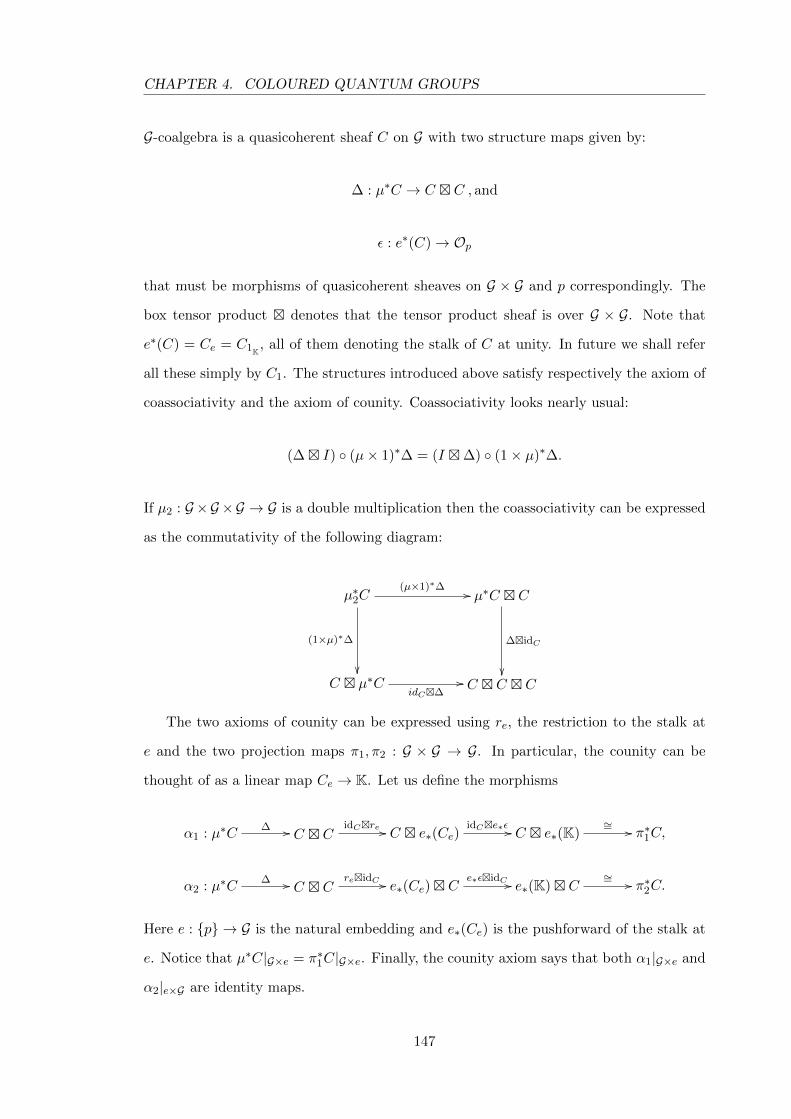
CHAPTER 4. COLOURED QUANTUM GROUPS
G-coalgebra is a quasicoherent sheaf C on G with two structure maps given by:
∆ : µ∗C → C � C , and
ε : e∗(C)→ Op
that must be morphisms of quasicoherent sheaves on G × G and p correspondingly. The
box tensor product � denotes that the tensor product sheaf is over G × G. Note that
e∗(C) = Ce = C1K, all of them denoting the stalk of C at unity. In future we shall refer
all these simply by C1. The structures introduced above satisfy respectively the axiom of
coassociativity and the axiom of counity. Coassociativity looks nearly usual:
(∆� I) ◦ (µ× 1)∗∆ = (I �∆) ◦ (1× µ)∗∆.
If µ2 : G ×G ×G → G is a double multiplication then the coassociativity can be expressed
as the commutativity of the following diagram:
µ∗2C(µ×1)∗∆ //
(1×µ)∗∆
��
µ∗C � C
∆�idC
��C � µ∗C
idC�∆// C � C � C
The two axioms of counity can be expressed using re, the restriction to the stalk at
e and the two projection maps π1, π2 : G × G → G. In particular, the counity can be
thought of as a linear map Ce → K. Let us define the morphisms
α1 : µ∗C∆ // C � C
idC�re // C � e∗(Ce)idC�e∗ε // C � e∗(K)
∼= // π∗1C,
α2 : µ∗C∆ // C � C
re�idC // e∗(Ce)� Ce∗ε�idC // e∗(K)� C
∼= // π∗2C.
Here e : {p} → G is the natural embedding and e∗(Ce) is the pushforward of the stalk at
e. Notice that µ∗C|G×e = π∗1C|G×e. Finally, the counity axiom says that both α1|G×e and
α2|e×G are identity maps.
147
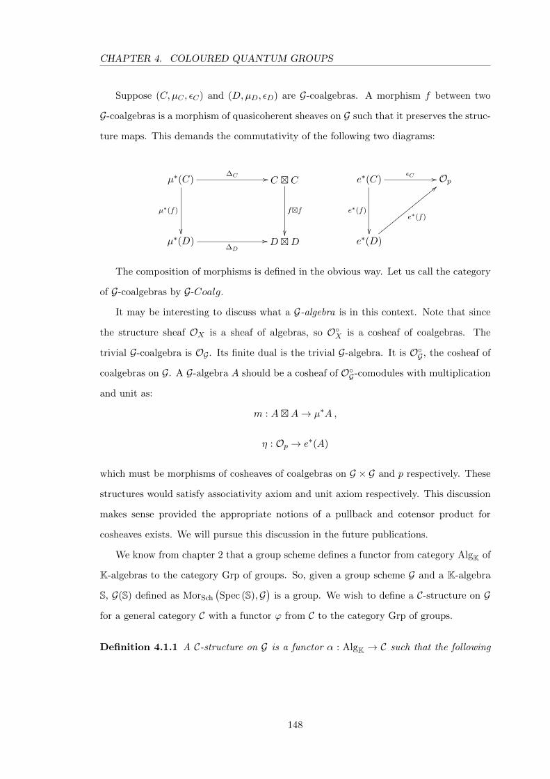
CHAPTER 4. COLOURED QUANTUM GROUPS
Suppose (C, µC , εC) and (D,µD, εD) are G-coalgebras. A morphism f between two
G-coalgebras is a morphism of quasicoherent sheaves on G such that it preserves the struc-
ture maps. This demands the commutativity of the following two diagrams:
µ∗(C)
µ∗(f)
��
∆C // C � C
f�f
��µ∗(D)
∆D
// D �D
e∗(C)
e∗(f)
��
εC // Op
e∗(D)
e∗(f)
<<yyyyyyyyyyyyyyyyy
The composition of morphisms is defined in the obvious way. Let us call the category
of G-coalgebras by G-Coalg.
It may be interesting to discuss what a G-algebra is in this context. Note that since
the structure sheaf OX is a sheaf of algebras, so O◦X is a cosheaf of coalgebras. The
trivial G-coalgebra is OG . Its finite dual is the trivial G-algebra. It is O◦G , the cosheaf of
coalgebras on G. A G-algebra A should be a cosheaf of O◦G-comodules with multiplication
and unit as:
m : A�A→ µ∗A ,
η : Op → e∗(A)
which must be morphisms of cosheaves of coalgebras on G × G and p respectively. These
structures would satisfy associativity axiom and unit axiom respectively. This discussion
makes sense provided the appropriate notions of a pullback and cotensor product for
cosheaves exists. We will pursue this discussion in the future publications.
We know from chapter 2 that a group scheme defines a functor from category AlgK of
K-algebras to the category Grp of groups. So, given a group scheme G and a K-algebra
S, G(S) defined as MorSch
(Spec (S),G
)is a group. We wish to define a C-structure on G
for a general category C with a functor ϕ from C to the category Grp of groups.
Definition 4.1.1 A C-structure on G is a functor α : AlgK → C such that the following
148
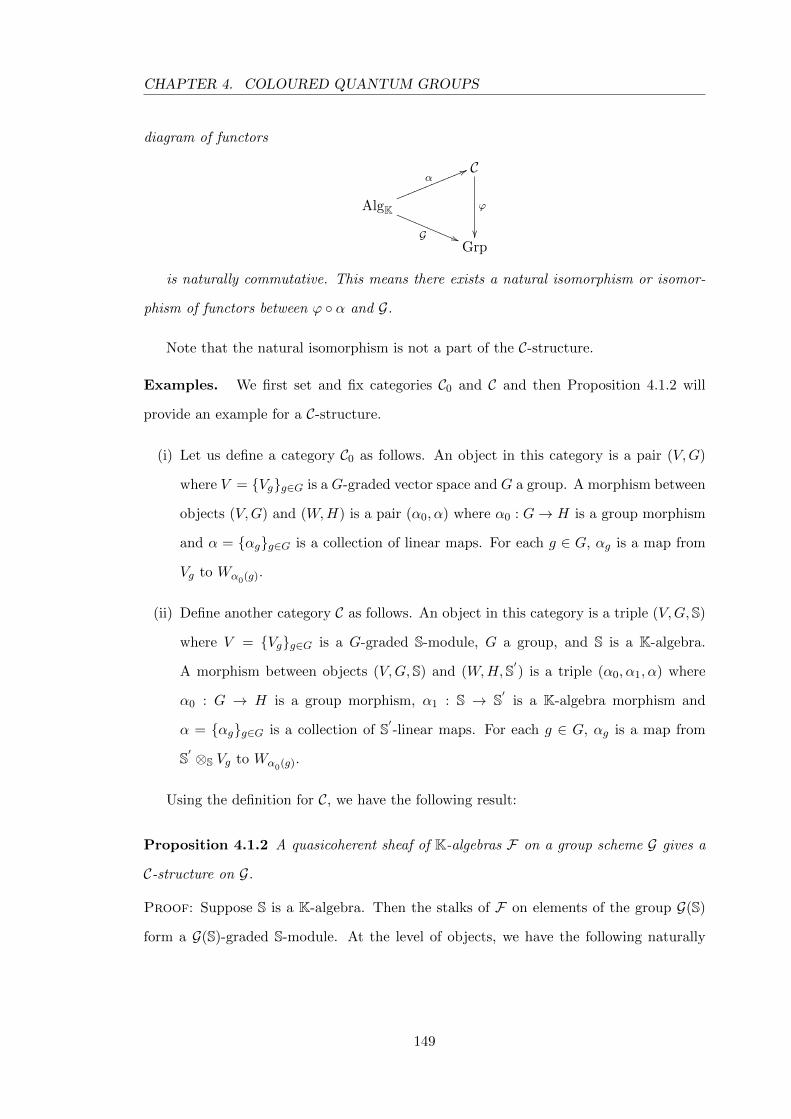
CHAPTER 4. COLOURED QUANTUM GROUPS
diagram of functors
C
ϕ
��
AlgK
G ((RRRRRRRRRR
α66llllllllllll
Grp
is naturally commutative. This means there exists a natural isomorphism or isomor-
phism of functors between ϕ ◦ α and G.
Note that the natural isomorphism is not a part of the C-structure.
Examples. We first set and fix categories C0 and C and then Proposition 4.1.2 will
provide an example for a C-structure.
(i) Let us define a category C0 as follows. An object in this category is a pair (V,G)
where V = {Vg}g∈G is a G-graded vector space and G a group. A morphism between
objects (V,G) and (W,H) is a pair (α0, α) where α0 : G→ H is a group morphism
and α = {αg}g∈G is a collection of linear maps. For each g ∈ G, αg is a map from
Vg to Wα0(g).
(ii) Define another category C as follows. An object in this category is a triple (V,G, S)
where V = {Vg}g∈G is a G-graded S-module, G a group, and S is a K-algebra.
A morphism between objects (V,G, S) and (W,H,S′) is a triple (α0, α1, α) where
α0 : G → H is a group morphism, α1 : S → S′ is a K-algebra morphism and
α = {αg}g∈G is a collection of S′-linear maps. For each g ∈ G, αg is a map from
S′ ⊗S Vg to Wα0(g).
Using the definition for C, we have the following result:
Proposition 4.1.2 A quasicoherent sheaf of K-algebras F on a group scheme G gives a
C-structure on G.
Proof: Suppose S is a K-algebra. Then the stalks of F on elements of the group G(S)
form a G(S)-graded S-module. At the level of objects, we have the following naturally
149
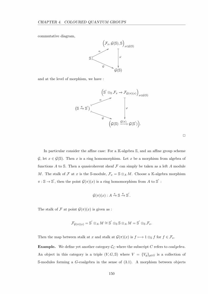
CHAPTER 4. COLOURED QUANTUM GROUPS
commutative diagram, (Fx,G(S), S
)x∈G(S)_
ϕ
��
S �
G ((QQQQQQQQQQQQQQ/
α77ooooooooooo
G(S)
and at the level of morphism, we have :
(S′ ⊗S Fx −→ FG(π)(x)
)x∈G(S)_
ϕ
��
(S π−→ S′
)�
G ))SSSSSSSSSSSSS
+α
55kkkkkkkkkkkkk
(G(S)
G(π)−−−→ G(S′)).
2
In particular consider the affine case: For a K-algebra S, and an affine group scheme
G, let x ∈ G(S). Then x is a ring homomorphism. Let x be a morphism from algebra of
functions A to S. Then a quasicoherent sheaf F can simply be taken as a left A module
M . The stalk of F at x is the S-module, Fx = S ⊗AM . Choose a K-algebra morphism
π : S→ S′ , then the point G(π)(x) is a ring homomorphism from A to S′ :
G(π)(x) : Ax−→ S π−→ S
′.
The stalk of F at point G(π)(x) is given as :
FG(π)(x) = S′ ⊗AM ∼= S
′ ⊗S S⊗AM = S′ ⊗S Fx.
Then the map between stalk at x and stalk at G(π)(x) is f 7−→ 1⊗S f for f ∈ Fx.
Example. We define yet another category CC where the subscript C refers to coalgebra.
An object in this category is a triple (V,G, S) where V = {Vg}g∈G is a collection of
S-modules forming a G-coalgebra in the sense of (3.1). A morphism between objects
150
CHAPTER 4. COLOURED QUANTUM GROUPS
(V,G, S) and (W,H,S′) is a triple (ρ0, ρ1, ρ) where ρ0 : G → H is a group homo-
morphism, ρ1 : S → S′ is a K-algebra morphism and ρ is a collection of S′-module
maps preserving the G-coalgebra structures, ı.e. ρ : S′ ⊗ V → ρ∗0(W ) is a morphism
of G-coalgebras over S′ . Note that for each g ∈ G, S′ ⊗S Vg is an S′-module, and
{S′ ⊗S Vg}g∈G forms a G-coalgebra over S′ . Again for each g ∈ G,(ρ∗0(W )
)g
= Wρ0(g)
and the collection ρ∗0(W ) ={Wρ0(g)
}g∈G
forms a G-coalgebra of S′-modules. Thus
ρ = {ρg : S′ ⊗S Vg −→Wρ0(g)}g∈G is the required collection of homomorphisms.
Given a G-coalgebra F on a group scheme G, we have a functor α : AlgK → CC taking
an object S to (Fx,G(S))x∈G(R), and a morphism π : S → S′ to (Fx → FG(π)(x))x∈G(S).
There is another functor ϕ : CC → Grp taking an object (V,G) to G, and a morphism
f = (f1, f2) : (V,G) → (W,H) to the group morphism f2 : G → H. Using this data, we
have the following result.
Proposition 4.1.3 A G-coalgebra on a group scheme G gives a CC-structure on G.
Proof: Let S be a K-algebra and let F be a G-coalgebra. We claim that the collection of
stalks of F on elements of the group G(S) form a G(S)-coalgebra. Let us also denote this
collection by F = {Fx}x∈G, where G = G(S). Now the comultiplication ∆ : µ∗F → F�F
of the sheaf F at the level of a stalk at (g, h) ∈ G×G looks like:
∆g,h : Fgh → Fg � Fh,
and the counit ε : e∗(F)→ Op at the level of a stalk at {p} is the following map:
ε : F1 → S
Note that the stalk of µ∗F at (g, h) is Fµ(g,h) = Fgh. Moreover, Fg � Fh is the stalk of
the sheaf F � F at (g, h). Further, Op(p) = OSpecK(SpecK) = K. At the level of objects
and morphism, we have the following naturally commutative diagrams,
151
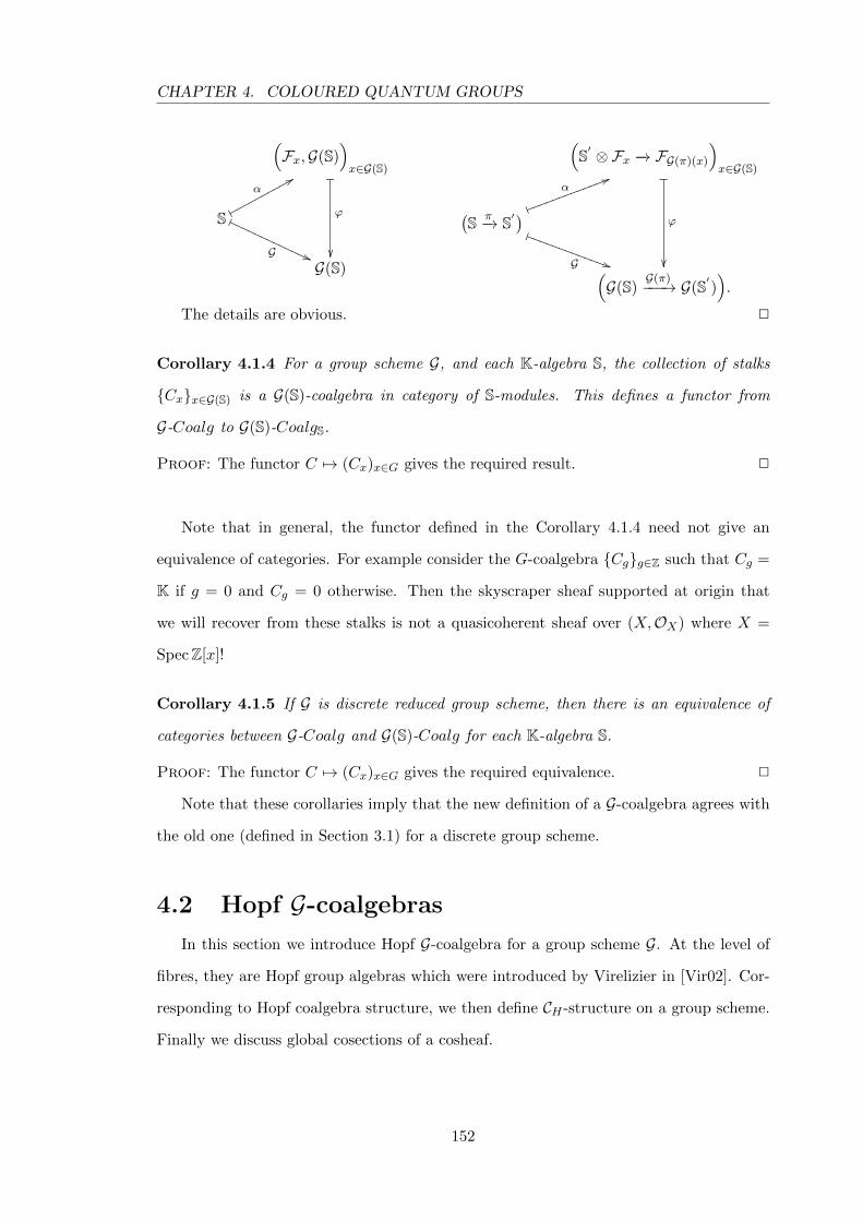
CHAPTER 4. COLOURED QUANTUM GROUPS
(Fx,G(S)
)x∈G(S)_
ϕ
��
S �
G ((PPPPPPPPPPPPP0
α88pppppppppp
G(S)
(S′ ⊗Fx −→ FG(π)(x)
)x∈G(S)_
ϕ
��
(S π−→ S′
)�
G ))SSSSSSSSSSSSS
+α
55kkkkkkkkkkkkk
(G(S)
G(π)−−−→ G(S′)).
The details are obvious. 2
Corollary 4.1.4 For a group scheme G, and each K-algebra S, the collection of stalks
{Cx}x∈G(S) is a G(S)-coalgebra in category of S-modules. This defines a functor from
G-Coalg to G(S)-CoalgS.
Proof: The functor C 7→ (Cx)x∈G gives the required result. 2
Note that in general, the functor defined in the Corollary 4.1.4 need not give an
equivalence of categories. For example consider the G-coalgebra {Cg}g∈Z such that Cg =
K if g = 0 and Cg = 0 otherwise. Then the skyscraper sheaf supported at origin that
we will recover from these stalks is not a quasicoherent sheaf over (X,OX) where X =
SpecZ[x]!
Corollary 4.1.5 If G is discrete reduced group scheme, then there is an equivalence of
categories between G-Coalg and G(S)-Coalg for each K-algebra S.
Proof: The functor C 7→ (Cx)x∈G gives the required equivalence. 2
Note that these corollaries imply that the new definition of a G-coalgebra agrees with
the old one (defined in Section 3.1) for a discrete group scheme.
4.2 Hopf G-coalgebras
In this section we introduce Hopf G-coalgebra for a group scheme G. At the level of
fibres, they are Hopf group algebras which were introduced by Virelizier in [Vir02]. Cor-
responding to Hopf coalgebra structure, we then define CH -structure on a group scheme.
Finally we discuss global cosections of a cosheaf.
152
CHAPTER 4. COLOURED QUANTUM GROUPS
4.2.1 Hopf group-coalgebras
In this section we discuss the definition of a Hopf group-coalgebra discussed by various
authors including Ohtsuki [Oht93], V.Turaev [Tur99] and Virelizier [Vir02]. Let P be a
multiplicative group with identity element e. A Hopf group-coalgebra, (in our case a Hopf
P -coalgebra) is a datum ({Ap}, {∆p,q}, {Sp}, ε) with p, q ∈ P . Each Ap is an K-algebra
(associative and unitary by default), the algebra morphisms ∆p,q : Apq → Ap ⊗ Aq form
a comultiplication, the linear maps Sp : Ap → Ap−1 form an antipode, and finally the
algebra morphism ε : Ae → K is a counit for the system. Denoting the algebra operations
in Ap by mp : Ap ⊗ Ap → Ap and ip : K → Ap the structure maps should satisfy the
following axioms.
(1) (id⊗∆p2,p3) ◦∆p1,p2p3 = (∆p1,p2 ⊗ id) ◦∆p1p2,p3 : Ap1p2p3 → Ap1 ⊗Ap2 ⊗Ap3(2) (id⊗ ε) ◦∆p,e = id : Ap → Ap
(3) (ε⊗ id) ◦∆e,p = id : Ap → Ap
(4) mp ◦ (id⊗ Sp−1) ◦∆p,p−1 = ip ◦ ε : Ae → Ap
(5) mp ◦ (Sp−1 ⊗ id) ◦∆p−1,p = ip ◦ ε : Ae → Ap
(6) ∆p,q and ε are homomorphisms of K algebras.
This definition has been given by Ohtsuki [Oht93] and he calls it a coloured Hopf
algebra over P . But there are three important differences from his definition. Firstly, he
demands the field to have characteristic zero and we don’t. Secondly, he demands the
group P to be abelian. Finally, he omits axiom (6), although all his examples satisfy it.
Note that axiom (6) is necessary if one wants to obtain the definition of a usual Hopf
algebra in the case of a trivial group P . The axiom (6) is required to conclude that
(Ae,∆e,e, Se, ε) is a Hopf algebra in the usual sense, which has been noted by Ohtsuki
as well. For simplicity we denote the collection ({Ap}, {∆p,q}, {Sp}, ε) by simply (Ap).
Ohtsuki has an example of a coloured Hopf algebra that he derives from a quantum group
Uq(sl2) at a root of unity, [Oht93]..
Given a group P , and two Hopf P -coalgebras {Ap,∆A, SA, εA} and {Bp,∆B, SB, εB},
we define a Hopf group coalgebra morphism φ between them as a collection φ = {φf :
Af → Bf}f∈P of algebra morphisms which respects all the structure morphisms of the
two. Explicitly, this demands the commutativity of the following diagrams:
153
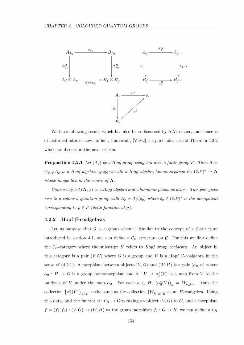
CHAPTER 4. COLOURED QUANTUM GROUPS
Afgφfg //
∆Afg
��
Bfg
∆Bfg
��Af ⊗Ag
φf⊗φg// Bf ⊗Bg
AfSAf //
φf
��
Af−1
φf−1
��Bf
SBf
// Bf−1
AeεA //
φe
��
K
Be
εB
==||||||||||||||||
We have following result, which has also been discussed by A.Virelizier, and hence is
of historical interest now. In fact, this result, [Vir02] is a particular case of Theorem 4.2.2
which we discuss in the next section.
Proposition 4.2.1 Let (Ap) be a Hopf group coalgebra over a finite group P . Then A =
⊕p∈PAp is a Hopf algebra equipped with a Hopf algebra homomorphism φ : (KP )∗ → A
whose image lies in the centre of A.
Conversely, let (A, φ) be a Hopf algebra and a homomorphism as above. This pair gives
rise to a coloured quantum group with Ap = Aφ(δp) where δp ∈ (KP )∗ is the idempotent
corresponding to p ∈ P (delta function at p).
4.2.2 Hopf G-coalgebras
Let us suppose that G is a group scheme. Similar to the concept of a C-structure
introduced in section 4.1, one can define a CH structure on G. For this we first define
the CH -category where the subscript H refers to Hopf group coalgebra. An object in
this category is a pair (V,G) where G is a group and V is a Hopf G-coalgebra in the
sense of (4.2.1). A morphism between objects (V,G) and (W,H) is a pair (α0, α) where
α0 : H → G is a group homomorphism and α : V → α∗0(V ) is a map from V to the
pullback of V under the map α0. For each h ∈ H,(α∗0(V )
)h
= Wα0(h) , thus the
collection{α∗0(V )
}h∈H is the same as the collection {Wh}h∈H as an H-coalgebra. Using
this data, and the functor ϕ : CH → Grp taking an object (V,G) to G, and a morphism
f = (f1, f2) : (V,G) → (W,H) to the group morphism f2 : G → H, we can define a CH
154
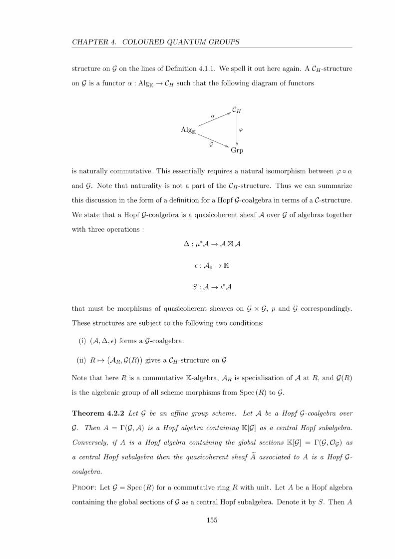
CHAPTER 4. COLOURED QUANTUM GROUPS
structure on G on the lines of Definition 4.1.1. We spell it out here again. A CH -structure
on G is a functor α : AlgK → CH such that the following diagram of functors
CH
ϕ
��
AlgK
G ((RRRRRRRRRR
α66lllllllllll
Grp
is naturally commutative. This essentially requires a natural isomorphism between ϕ ◦ α
and G. Note that naturality is not a part of the CH -structure. Thus we can summarize
this discussion in the form of a definition for a Hopf G-coalgebra in terms of a C-structure.
We state that a Hopf G-coalgebra is a quasicoherent sheaf A over G of algebras together
with three operations :
∆ : µ∗A → A�A
ε : Ae → K
S : A → ι∗A
that must be morphisms of quasicoherent sheaves on G × G, p and G correspondingly.
These structures are subject to the following two conditions:
(i) (A,∆, ε) forms a G-coalgebra.
(ii) R 7→(AR,G(R)
)gives a CH -structure on G
Note that here R is a commutative K-algebra, AR is specialisation of A at R, and G(R)
is the algebraic group of all scheme morphisms from Spec (R) to G.
Theorem 4.2.2 Let G be an affine group scheme. Let A be a Hopf G-coalgebra over
G. Then A = Γ(G,A) is a Hopf algebra containing K[G] as a central Hopf subalgebra.
Conversely, if A is a Hopf algebra containing the global sections K[G] = Γ(G,OG) as
a central Hopf subalgebra then the quasicoherent sheaf A associated to A is a Hopf G-
coalgebra.
Proof: Let G = Spec (R) for a commutative ring R with unit. Let A be a Hopf algebra
containing the global sections of G as a central Hopf subalgebra. Denote it by S. Then A
155
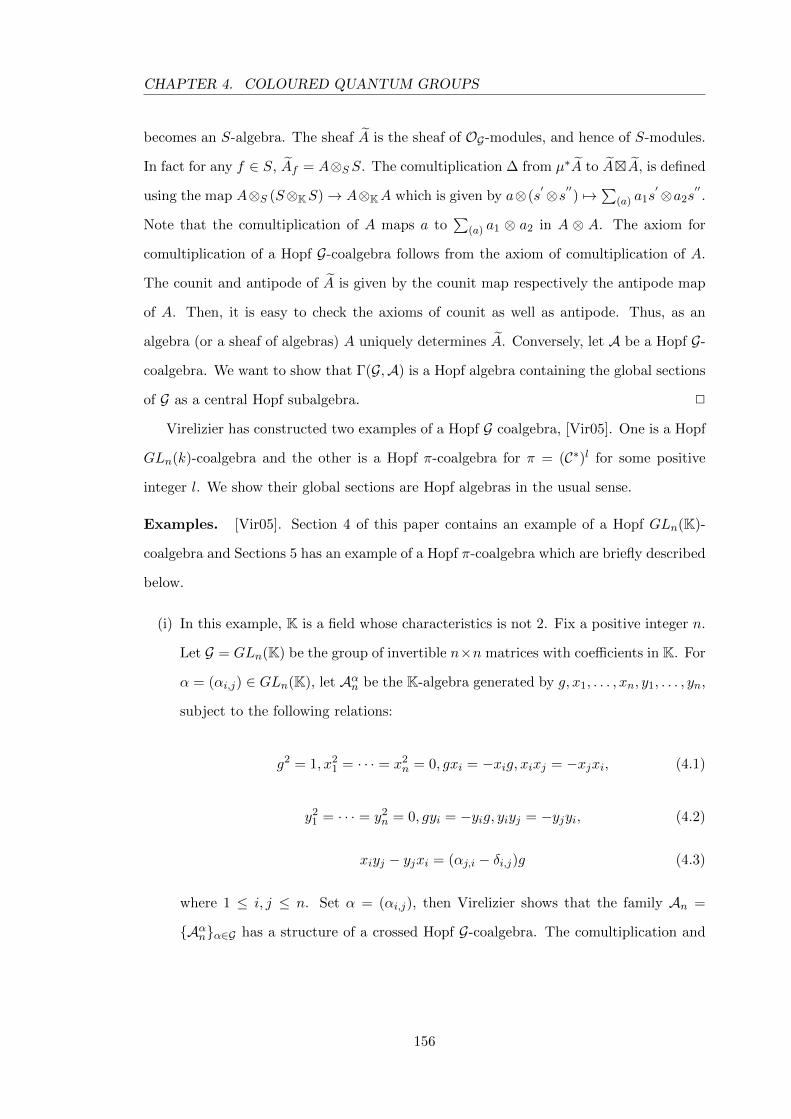
CHAPTER 4. COLOURED QUANTUM GROUPS
becomes an S-algebra. The sheaf A is the sheaf of OG-modules, and hence of S-modules.
In fact for any f ∈ S, Af = A⊗S S. The comultiplication ∆ from µ∗A to A�A, is defined
using the map A⊗S (S⊗KS)→ A⊗KA which is given by a⊗(s′⊗s′′) 7→
∑(a) a1s
′⊗a2s′′.
Note that the comultiplication of A maps a to∑
(a) a1 ⊗ a2 in A ⊗ A. The axiom for
comultiplication of a Hopf G-coalgebra follows from the axiom of comultiplication of A.
The counit and antipode of A is given by the counit map respectively the antipode map
of A. Then, it is easy to check the axioms of counit as well as antipode. Thus, as an
algebra (or a sheaf of algebras) A uniquely determines A. Conversely, let A be a Hopf G-
coalgebra. We want to show that Γ(G,A) is a Hopf algebra containing the global sections
of G as a central Hopf subalgebra. 2
Virelizier has constructed two examples of a Hopf G coalgebra, [Vir05]. One is a Hopf
GLn(k)-coalgebra and the other is a Hopf π-coalgebra for π = (C∗)l for some positive
integer l. We show their global sections are Hopf algebras in the usual sense.
Examples. [Vir05]. Section 4 of this paper contains an example of a Hopf GLn(K)-
coalgebra and Sections 5 has an example of a Hopf π-coalgebra which are briefly described
below.
(i) In this example, K is a field whose characteristics is not 2. Fix a positive integer n.
Let G = GLn(K) be the group of invertible n×n matrices with coefficients in K. For
α = (αi,j) ∈ GLn(K), let Aαn be the K-algebra generated by g, x1, . . . , xn, y1, . . . , yn,
subject to the following relations:
g2 = 1, x21 = · · · = x2
n = 0, gxi = −xig, xixj = −xjxi, (4.1)
y21 = · · · = y2
n = 0, gyi = −yig, yiyj = −yjyi, (4.2)
xiyj − yjxi = (αj,i − δi,j)g (4.3)
where 1 ≤ i, j ≤ n. Set α = (αi,j), then Virelizier shows that the family An =
{Aαn}α∈G has a structure of a crossed Hopf G-coalgebra. The comultiplication and
156
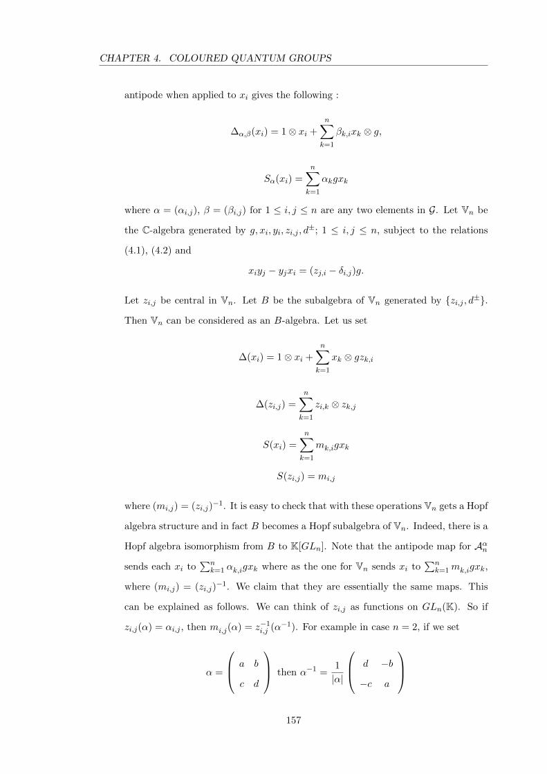
CHAPTER 4. COLOURED QUANTUM GROUPS
antipode when applied to xi gives the following :
∆α,β(xi) = 1⊗ xi +
n∑k=1
βk,ixk ⊗ g,
Sα(xi) =n∑k=1
αkgxk
where α = (αi,j), β = (βi,j) for 1 ≤ i, j ≤ n are any two elements in G. Let Vn be
the C-algebra generated by g, xi, yi, zi,j , d±; 1 ≤ i, j ≤ n, subject to the relations
(4.1), (4.2) and
xiyj − yjxi = (zj,i − δi,j)g.
Let zi,j be central in Vn. Let B be the subalgebra of Vn generated by {zi,j , d±}.
Then Vn can be considered as an B-algebra. Let us set
∆(xi) = 1⊗ xi +n∑k=1
xk ⊗ gzk,i
∆(zi,j) =n∑k=1
zi,k ⊗ zk,j
S(xi) =
n∑k=1
mk,igxk
S(zi,j) = mi,j
where (mi,j) = (zi,j)−1. It is easy to check that with these operations Vn gets a Hopf
algebra structure and in fact B becomes a Hopf subalgebra of Vn. Indeed, there is a
Hopf algebra isomorphism from B to K[GLn]. Note that the antipode map for Aαn
sends each xi to∑n
k=1 αk,igxk where as the one for Vn sends xi to∑n
k=1mk,igxk,
where (mi,j) = (zi,j)−1. We claim that they are essentially the same maps. This
can be explained as follows. We can think of zi,j as functions on GLn(K). So if
zi,j(α) = αi,j , then mi,j(α) = z−1i,j (α−1). For example in case n = 2, if we set
α =
a b
c d
then α−1 =1
|α|
d −b
−c a
157
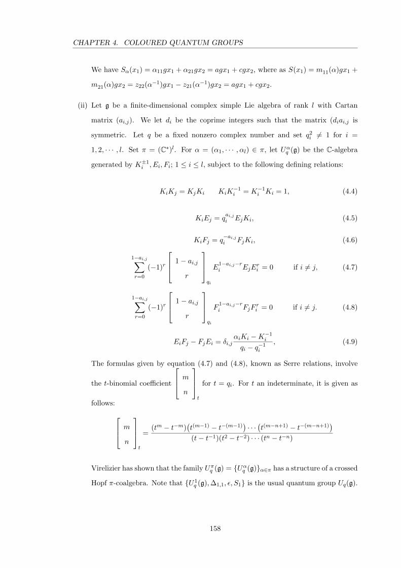
CHAPTER 4. COLOURED QUANTUM GROUPS
We have Sα(x1) = α11gx1 + α21gx2 = agx1 + cgx2, where as S(x1) = m11(α)gx1 +
m21(α)gx2 = z22(α−1)gx1 − z21(α−1)gx2 = agx1 + cgx2.
(ii) Let g be a finite-dimensional complex simple Lie algebra of rank l with Cartan
matrix (ai,j). We let di be the coprime integers such that the matrix (diai,j is
symmetric. Let q be a fixed nonzero complex number and set q2i 6= 1 for i =
1, 2, · · · , l. Set π = (C∗)l. For α = (α1, · · · , αl) ∈ π, let Uαq (g) be the C-algebra
generated by K±1i , Ei, Fi; 1 ≤ i ≤ l, subject to the following defining relations:
KiKj = KjKi KiK−1i = K−1
i Ki = 1, (4.4)
KiEj = qai,ji EjKi, (4.5)
KiFj = q−ai,ji FjKi, (4.6)
1−ai,j∑r=0
(−1)r
1− ai,j
r
qi
E1−ai,j−ri EjE
ri = 0 if i 6= j, (4.7)
1−ai,j∑r=0
(−1)r
1− ai,j
r
qi
F1−ai,j−ri FjF
ri = 0 if i 6= j. (4.8)
EiFj − FjEi = δi,jαiKi −K−1
i
qi − q−1i
, (4.9)
The formulas given by equation (4.7) and (4.8), known as Serre relations, involve
the t-binomial coefficient
m
n
t
for t = qi. For t an indeterminate, it is given as
follows: m
n
t
=(tm − t−m)
(t(m−1) − t−(m−1)
)· · ·(t(m−n+1) − t−(m−n+1)
)(t− t−1)(t2 − t−2) · · · (tn − t−n)
Virelizier has shown that the family Uπq (g) = {Uαq (g)}α∈π has a structure of a crossed
Hopf π-coalgebra. Note that {U1q (g),∆1,1, ε, S1} is the usual quantum group Uq(g).
158
CHAPTER 4. COLOURED QUANTUM GROUPS
The comultiplication and antipode when applied to Ei gives the following :
∆α,β(Ei) = βiEi ⊗Ki + 1⊗ Ei,
Sα(Ei) = −αiEiK−1i
where α = (αi,j), β = (βi,j); 1 ≤ i, j ≤ n are any two elements in G. As in
the previous example, let Uq(g) be the C-algebra generated by K±1i , Ei, Fi, Z
±i ;
1 ≤ i ≤ l, subject to the defining relations (4.4) to (4.8), and
EiFj − FjEi =ZiKi −K−1
i
qi − q−1i
.
Let Z±1i be central in Uq(g). Let C be the subalgebra of Uq(g) generated by {Z±1
i }.
Then Uq(g) can be considered as an C-algebra. Let us set
∆(Ei) = Ei ⊗ ZiKi + 1⊗ Ei
∆(Zi) = Zi ⊗ Zi
S(Ei) = −Z−1i EiK
−1i
S(Zi) = Z−1i
One can easily check that both Uq(g) and C forms a Hopf algebra with these oper-
ations. And there is a Hopf algebra isomorphism from C to K[π]. The explanation
for a slightly different antipode of Uq(g) than of {Uπq (g)} is similar to as explained
in the previous example.
Let G be the algebraic group G(S) for a commutative ring S and A be a Hopf G-
coalgebra. Then the specialisation of A at S forms a Hopf G-coalgebra.
Proposition 4.2.3 Given a group scheme G, and A a Hopf G-coalgebra, then the spe-
cialisation of A at S forms a Hopf G-coalgebra.
Proof: The proof follows from definition 7 (ii), of a Hopf G-coalgebra, which says that
(AS ,G(S)) is a Hopf G(S)-coalgebra, for any commutative K-algebra S. 2
159
CHAPTER 4. COLOURED QUANTUM GROUPS
Let AG be the category of Hopf G-coalgebras over a group scheme G and BG the
category of Hopf G-coalgebra over a group G. Let A be any object in AG . Then for any
commutative algebra S over K, its specialization AS is an object in BG(S). Thus we have
Proposition 4.2.4 For a commutative algebra S over K, there exists a functor
F : AG → BG(S).
By Supp(Af ) we understand the support of A at the fibre (Af ), i.e., the set of all
f ∈ G such that Af 6= 0. We have the following result.
Lemma 4.2.5 The support Supp(Af ) is a closed subgroup scheme of G.
Proof: The support is non-empty because Ae 6= 0 as ε : Ae → K is a homomorphism of
algebras. The closeness under multiplication and inverse follows from the axiom (6) and
(5) correspondingly. 2
4.2.3 Crossings
So far we have defined a G-coalgebra and a Hopf G-coalgebra. We now set up some
more structures to the list. We provide crossings to a Hopf G-coalgebra.
Consider a Hopf G-coalgebra A over a group scheme G. We can treat G as a G-variety
equipped with the conjugation action of G on itself. This admits a G-equivariant structure
on A (See chapter 1). Now on the same lines of the discrete case, [Tur00], [Vir02], we
say that A is a crossed Hopf G-coalgebra provided it is equipped with a G-equivariant
structure
ϕ : π∗1A → c∗A
where π1 is the first projection on G × G and c is the conjugation map on G. Note that
ϕ is an isomorphism of sheaves on G × G. The crossing must satisfy the following set of
axioms :
(i) ϕ is a homomorphism of sheaves of algebras over G × G.
(ii) ϕ preserves the comultiplication of A. This is given by the commutativity of the
160
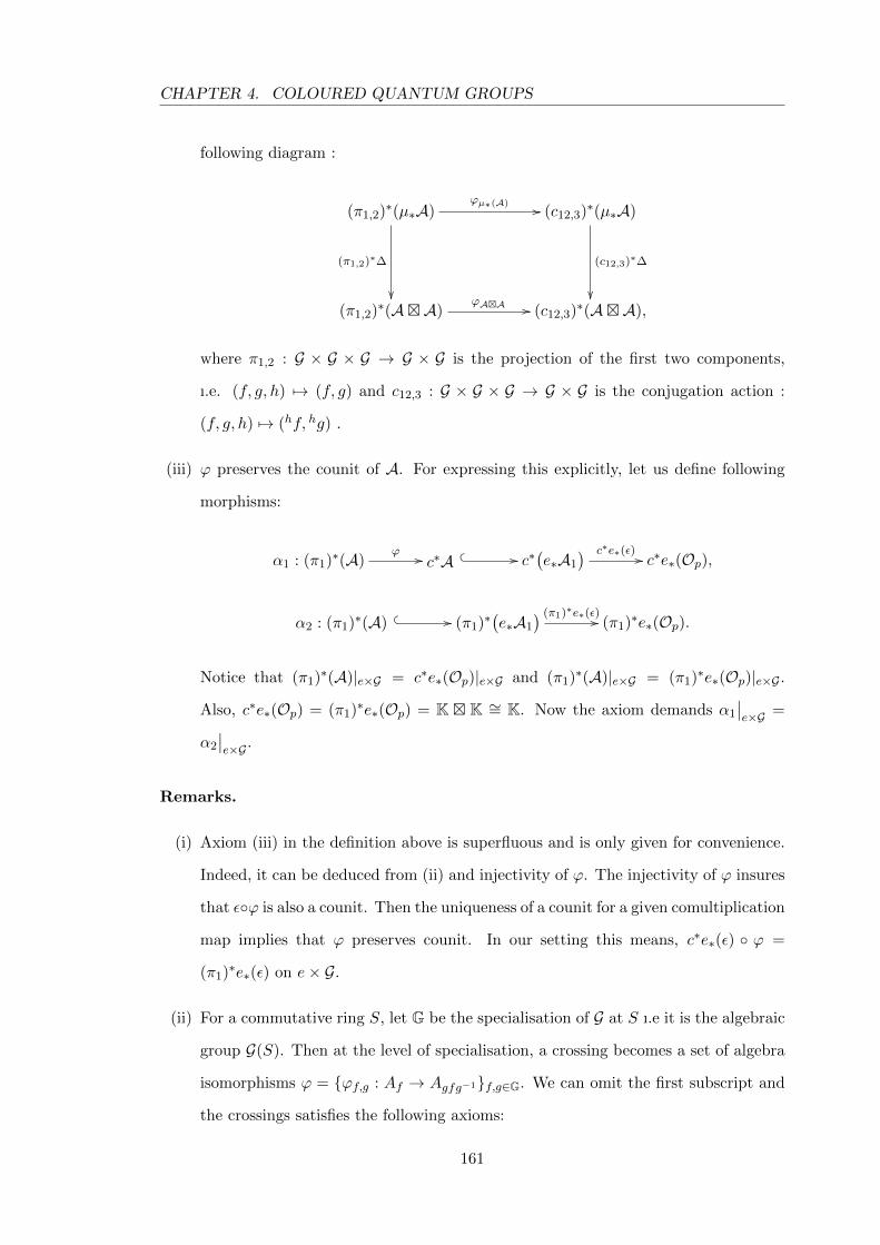
CHAPTER 4. COLOURED QUANTUM GROUPS
following diagram :
(π1,2)∗(µ∗A)
(π1,2)∗∆
��
ϕµ∗(A) // (c12,3)∗(µ∗A)
(c12,3)∗∆
��(π1,2)∗(A�A)
ϕA�A // (c12,3)∗(A�A),
where π1,2 : G × G × G → G × G is the projection of the first two components,
ı.e. (f, g, h) 7→ (f, g) and c12,3 : G × G × G → G × G is the conjugation action :
(f, g, h) 7→ (hf, hg) .
(iii) ϕ preserves the counit of A. For expressing this explicitly, let us define following
morphisms:
α1 : (π1)∗(A)ϕ // c∗A � � // c∗
(e∗A1
) c∗e∗(ε) // c∗e∗(Op),
α2 : (π1)∗(A) � � // (π1)∗(e∗A1
) (π1)∗e∗(ε)// (π1)∗e∗(Op).
Notice that (π1)∗(A)|e×G = c∗e∗(Op)|e×G and (π1)∗(A)|e×G = (π1)∗e∗(Op)|e×G .
Also, c∗e∗(Op) = (π1)∗e∗(Op) = K � K ∼= K. Now the axiom demands α1
∣∣e×G =
α2
∣∣e×G .
Remarks.
(i) Axiom (iii) in the definition above is superfluous and is only given for convenience.
Indeed, it can be deduced from (ii) and injectivity of ϕ. The injectivity of ϕ insures
that ε◦ϕ is also a counit. Then the uniqueness of a counit for a given comultiplication
map implies that ϕ preserves counit. In our setting this means, c∗e∗(ε) ◦ ϕ =
(π1)∗e∗(ε) on e× G.
(ii) For a commutative ring S, let G be the specialisation of G at S ı.e it is the algebraic
group G(S). Then at the level of specialisation, a crossing becomes a set of algebra
isomorphisms ϕ = {ϕf,g : Af → Agfg−1}f,g∈G. We can omit the first subscript and
the crossings satisfies the following axioms:
161
CHAPTER 4. COLOURED QUANTUM GROUPS
• ϕ is multiplicative ı.e., ϕf ◦ ϕg = ϕfg , for any f, g ∈ G.
• ϕ is compatible with ∆ ı.e, ∆hfh−1,hgh−1 ◦ ϕh = (ϕh ⊗ ϕh) ◦ ∆f,g , for any
f, g, h ∈ G.
• ϕ is compatible with ε ı.e, ε ◦ ϕf = ε , for any f ∈ G.
All these three properties follows by specialising the axioms of a crossings at S thus
giving a crossed Hopf G-coalgebra A = {Ag}g∈G as defined by Virelizier [Vir02].
(iii) It follows that for any g ∈ G, ϕg,e : Ag → Ag is an identity map using the multi-
plicativity of ϕ.
Examples. The two examples of Hopf G-coalgebras discussed in section 4.2.1 are crossed.
We give here the formula for the crossing for the two examples, [Vir05].
(i) Vn: The family An of Hopf GLn(K)-coalgebra as discussed in last section is crossed.
The crossings are given by the following formulae:
ϕα(g) = g, ϕα(xi) =
n∑k=1
αk,ixk, ϕα(yi) =
n∑k=1
αk,iyk
(ii) Uq: The family Uπq (g) = {Uαq (g)}α∈π is a crossed Hopf π-coalgebra. The crossings
are given by:
ϕα(Ki) = Ki, ϕα(Ei) = αiEi, ϕα(Fi) = α−1i Fi.
4.2.4 Quasitriangularity
Given a crossed Hopf G-coalgebra A, we now provide it with a quasi-triangular struc-
ture. First let us define a universal R-matrix for A as the sheaf over G × G of invertible
points in the global section ı.e
R ∈ Γ(G,A)⊗K Γ(G,A) ⊆ Γ(G × G,A�A)
such that for any open U × V ⊆ G × G, R(U × V ) is an invertible element in the alge-
bra Γ(G,A) ⊗K Γ((G,A). Thus at the level of specialisation, when G = G(S) for some
162
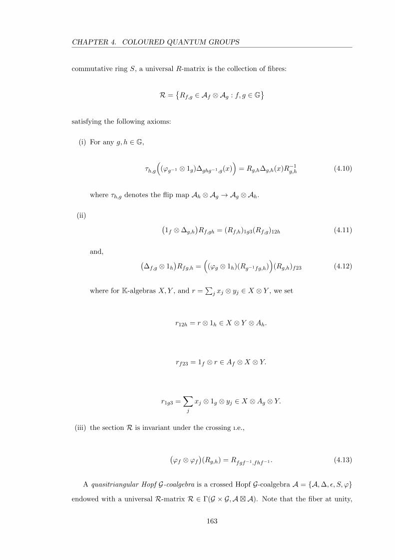
CHAPTER 4. COLOURED QUANTUM GROUPS
commutative ring S, a universal R-matrix is the collection of fibres:
R ={Rf,g ∈ Af ⊗Ag : f, g ∈ G
}satisfying the following axioms:
(i) For any g, h ∈ G,
τh,g
((ϕg−1 ⊗ 1g)∆ghg−1,g(x)
)= Rg,h∆g,h(x)R−1
g,h (4.10)
where τh,g denotes the flip map Ah ⊗Ag → Ag ⊗Ah.
(ii) (1f ⊗∆g,h
)Rf,gh = (Rf,h)1g3(Rf,g)12h (4.11)
and, (∆f,g ⊗ 1h
)Rfg,h =
((ϕg ⊗ 1h)(Rg−1fg,h)
)(Rg,h)f23 (4.12)
where for K-algebras X,Y , and r =∑
j xj ⊗ yj ∈ X ⊗ Y , we set
r12h = r ⊗ 1h ∈ X ⊗ Y ⊗Ah.
rf23 = 1f ⊗ r ∈ Af ⊗X ⊗ Y.
r1g3 =∑j
xj ⊗ 1g ⊗ yj ∈ X ⊗Ag ⊗ Y.
(iii) the section R is invariant under the crossing ı.e.,
(ϕf ⊗ ϕf
)(Rg,h) = Rfgf−1,fhf−1 . (4.13)
A quasitriangular Hopf G-coalgebra is a crossed Hopf G-coalgebra A = {A,∆, ε, S, ϕ}
endowed with a universal R-matrix R ∈ Γ(G × G,A � A). Note that the fiber at unity,
163
CHAPTER 4. COLOURED QUANTUM GROUPS
Re,e is the classical R-matrix for the Hopf algebra Ae since ϕe = Id by remark (iii) of last
section. In case G is also an abelian group and the crossings ϕ happen to be trivial (that
is ϕh|Ag = 1g for all g, h ∈ G ), one recovers the definition of a quasitriangular coloured
Hopf algebra given by Ohtsuki for the discrete case, [Oht93] .
Example. The family An of crossed Hopf GLn(K)-coalgebra as discussed in last section
is quasitriangular. The R-matrix is given, for α, β ∈ GLn(K), by:
Rα,β =1
2
∑S⊆[n]
xS ⊗ yS + xS ⊗ gyS + gxS ⊗ yS − gxS ⊗ gyS .
Here [n] = {1, · · ·n}, x∅ = 1, y∅ = 1 and for a nonempty subset S of n we let xS =
xi1 · · ·xiS and yS = yi1 · · · yiS where i1 < · · · < iS are the elements of S.
Note that the family Uπq (g) = {Uαq (g)}α∈π which is a crossed Hopf π-coalgebra is not
quasitriangular in general. Indeed, it is topologically quasitriangular so that the universal
R-matrix will lie in the completion of the external tensor product of the sheafA with itself.
Note that usual Uq(g) is not quasitriangular either. Since R lies in some completeion of
Uq(g)⊗ Uq(g) rather than in Uq(g)⊗ Uq(g) itself. Drinfeld gives an expression for R as a
power series in tensor products of the generators of Uq(g), [Dri87] .
4.3 Affine case
In this section, we shall assume that the underlying group scheme is affine. Let
G = Spec (H) for a commutative K-Hopf algebra H. This helps us to elaborate the dual
of a Hopf G-coalgebra, crossings for a Hopf G-coalgebra and thus formulate the quantum
double explicitly.
4.3.1 Structure of a Hopf G-coalgebra
A quasicoherent sheaf A of algebras over the affine group scheme G is simply a quasi-
coherent sheaf A where A is an H-algebra with the action of H on A given via − : H → A.
At any topological point f ∈ G, the stalk of A at f is A(f) = H(f)⊗H A where H(f) is the
localisation of H at the point f (which is essentially an ideal). Let S be a commutative
K-algebra. Considering G as a functor, the fiber of A over any algebraic point f : H → S
164
CHAPTER 4. COLOURED QUANTUM GROUPS
is S ⊗H A. Note that S is an H-module via the map f . From here onwards we choose
the notation S ⊗f A to refer to the fiber of A at the algebraic point f : H → S. Now
given that the sheaf A is a Hopf G-coalgebra implies that it is equipped with following
structure maps which can be visualised explicitly at the level of fibres :
∆f,g : S⊗µ(f,g) A→ S⊗f A⊗S S⊗g A
ε : S⊗1 A→ S
Sf : S⊗f A→ S⊗f−1 A
where f, f−1, g, 1 : H → S are all algebraic points in G(S) with f−1 : H → S is such that
f(x1)f−1(x2) = ε(x).1S and 1 = ηS ◦ εH .
Globally, the structures ∆ and ε are morphisms of algebras such that they satisfy
respectively the axiom of coassociativity and the axiom of counity. Note that at global
level, Γ(G, A) = A, and by Theorem (4.2.2) A is essentially a Hopf algebra over K.
4.3.2 Crossings
The Hopf G-coalgebra sheaf A is crossed implies that it is equipped with following
isomorphisms of algebras (called crossings), which at the level of fibres is given as :
ϕg : S⊗f A→ S⊗c(f,g) A.
Note that c(f, g) = gfg−1 : H → S is again an algebraic point of G defined as x 7→
g(x1)f(x2)g−1(x3), where g−1(y) = g(Sy). These crossings satisfy the following two
axioms:
(i) ϕ preserves comultiplication of A. This can be expressed at fiber-level by the fol-
lowing diagram:
165
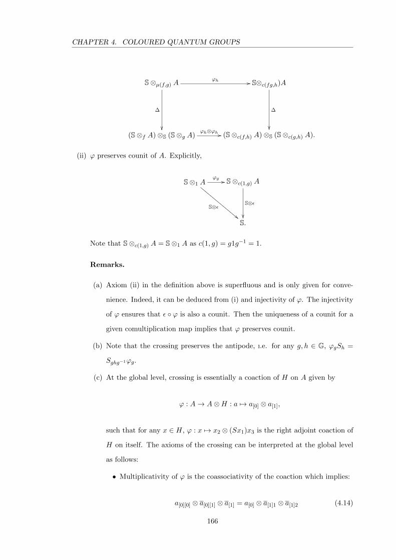
CHAPTER 4. COLOURED QUANTUM GROUPS
S⊗µ(f,g) A
∆
��
ϕh // S⊗c(fg,h)A
∆
��(S⊗f A)⊗S (S⊗g A)
ϕh⊗ϕh // (S⊗c(f,h) A)⊗S (S⊗c(g,h) A).
(ii) ϕ preserves counit of A. Explicitly,
S⊗1 A
S⊗ε
""DDDDDDDDDDDDDDDϕg // S⊗c(1,g) A
S⊗ε
��S.
Note that S⊗c(1,g) A = S⊗1 A as c(1, g) = g1g−1 = 1.
Remarks.
(a) Axiom (ii) in the definition above is superfluous and is only given for conve-
nience. Indeed, it can be deduced from (i) and injectivity of ϕ. The injectivity
of ϕ ensures that ε ◦ ϕ is also a counit. Then the uniqueness of a counit for a
given comultiplication map implies that ϕ preserves counit.
(b) Note that the crossing preserves the antipode, ı.e. for any g, h ∈ G, ϕgSh =
Sghg−1ϕg.
(c) At the global level, crossing is essentially a coaction of H on A given by
ϕ : A→ A⊗H : a 7→ a[0] ⊗ a[1],
such that for any x ∈ H, ϕ : x 7→ x2 ⊗ (Sx1)x3 is the right adjoint coaction of
H on itself. The axioms of the crossing can be interpreted at the global level
as follows:
• Multiplicativity of ϕ is the coassociativity of the coaction which implies:
a[0][0] ⊗ a[0][1] ⊗ a[1] = a[0] ⊗ a[1]1 ⊗ a[1]2 (4.14)
166
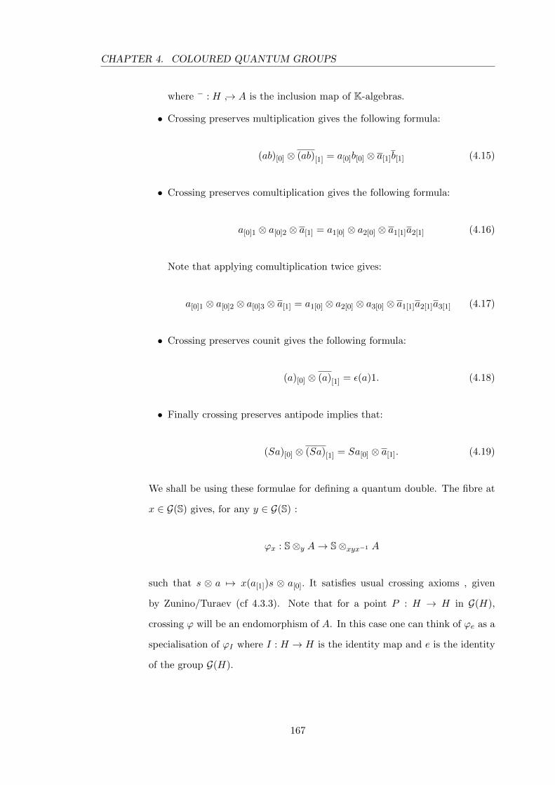
CHAPTER 4. COLOURED QUANTUM GROUPS
where − : H ↪→ A is the inclusion map of K-algebras.
• Crossing preserves multiplication gives the following formula:
(ab)[0] ⊗ (ab)[1] = a[0]b[0] ⊗ a[1]b[1] (4.15)
• Crossing preserves comultiplication gives the following formula:
a[0]1 ⊗ a[0]2 ⊗ a[1] = a1[0] ⊗ a2[0] ⊗ a1[1]a2[1] (4.16)
Note that applying comultiplication twice gives:
a[0]1 ⊗ a[0]2 ⊗ a[0]3 ⊗ a[1] = a1[0] ⊗ a2[0] ⊗ a3[0] ⊗ a1[1]a2[1]a3[1] (4.17)
• Crossing preserves counit gives the following formula:
(a)[0] ⊗ (a)[1] = ε(a)1. (4.18)
• Finally crossing preserves antipode implies that:
(Sa)[0] ⊗ (Sa)[1] = Sa[0] ⊗ a[1]. (4.19)
We shall be using these formulae for defining a quantum double. The fibre at
x ∈ G(S) gives, for any y ∈ G(S) :
ϕx : S⊗y A→ S⊗xyx−1 A
such that s ⊗ a 7→ x(a[1])s ⊗ a[0]. It satisfies usual crossing axioms , given
by Zunino/Turaev (cf 4.3.3). Note that for a point P : H → H in G(H),
crossing ϕ will be an endomorphism of A. In this case one can think of ϕe as a
specialisation of ϕI where I : H → H is the identity map and e is the identity
of the group G(H).
167
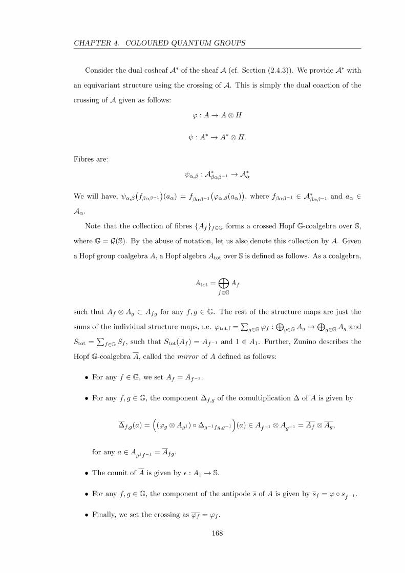
CHAPTER 4. COLOURED QUANTUM GROUPS
Consider the dual cosheaf A∗ of the sheaf A (cf. Section (2.4.3)). We provide A∗ with
an equivariant structure using the crossing of A. This is simply the dual coaction of the
crossing of A given as follows:
ϕ : A→ A⊗H
ψ : A∗ → A∗ ⊗H.
Fibres are:
ψα,β : A∗βαβ−1 → A∗α
We will have, ψα,β(fβαβ−1
)(aα) = fβαβ−1
(ϕα,β(aα)
), where fβαβ−1 ∈ A∗βαβ−1 and aα ∈
Aα.
Note that the collection of fibres {Af}f∈G forms a crossed Hopf G-coalgebra over S,
where G = G(S). By the abuse of notation, let us also denote this collection by A. Given
a Hopf group coalgebra A, a Hopf algebra Atot over S is defined as follows. As a coalgebra,
Atot =⊕f∈G
Af
such that Af ⊗ Ag ⊂ Afg for any f, g ∈ G. The rest of the structure maps are just the
sums of the individual structure maps, ı.e. ϕtot,f =∑
g∈G ϕf :⊕
g∈GAg 7→⊕
g∈GAg and
Stot =∑
f∈G Sf , such that Stot(Af ) = Af−1 and 1 ∈ A1. Further, Zunino describes the
Hopf G-coalgebra A, called the mirror of A defined as follows:
• For any f ∈ G, we set Af = Af−1 .
• For any f, g ∈ G, the component ∆f,g of the comultiplication ∆ of A is given by
∆f,g(a) =(
(ϕg ⊗Ag1) ◦∆g−1fg,g−1
)(a) ∈ Af−1 ⊗Ag−1 = Af ⊗Ag,
for any a ∈ Ag1f−1 = Afg.
• The counit of A is given by ε : A1 → S.
• For any f, g ∈ G, the component of the antipode s of A is given by sf = ϕ ◦ sf−1 .
• Finally, we set the crossing as ϕf = ϕf .
168
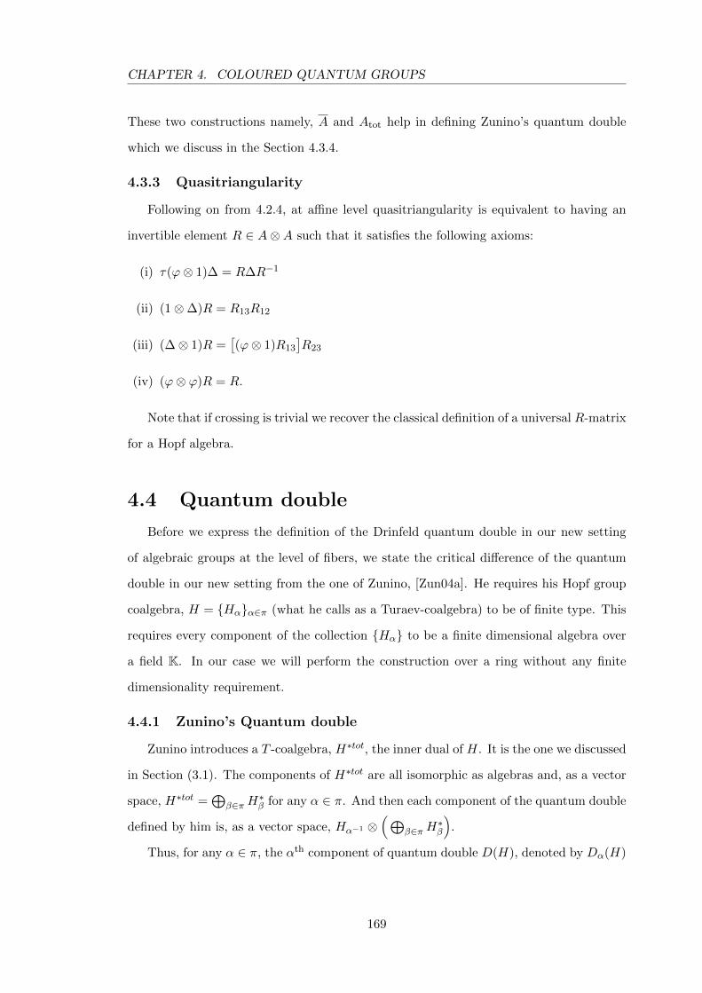
CHAPTER 4. COLOURED QUANTUM GROUPS
These two constructions namely, A and Atot help in defining Zunino’s quantum double
which we discuss in the Section 4.3.4.
4.3.3 Quasitriangularity
Following on from 4.2.4, at affine level quasitriangularity is equivalent to having an
invertible element R ∈ A⊗A such that it satisfies the following axioms:
(i) τ(ϕ⊗ 1)∆ = R∆R−1
(ii) (1⊗∆)R = R13R12
(iii) (∆⊗ 1)R =[(ϕ⊗ 1)R13
]R23
(iv) (ϕ⊗ ϕ)R = R.
Note that if crossing is trivial we recover the classical definition of a universal R-matrix
for a Hopf algebra.
4.4 Quantum double
Before we express the definition of the Drinfeld quantum double in our new setting
of algebraic groups at the level of fibers, we state the critical difference of the quantum
double in our new setting from the one of Zunino, [Zun04a]. He requires his Hopf group
coalgebra, H = {Hα}α∈π (what he calls as a Turaev-coalgebra) to be of finite type. This
requires every component of the collection {Hα} to be a finite dimensional algebra over
a field K. In our case we will perform the construction over a ring without any finite
dimensionality requirement.
4.4.1 Zunino’s Quantum double
Zunino introduces a T -coalgebra, H∗tot, the inner dual of H. It is the one we discussed
in Section (3.1). The components of H∗tot are all isomorphic as algebras and, as a vector
space, H∗tot =⊕
β∈πH∗β for any α ∈ π. And then each component of the quantum double
defined by him is, as a vector space, Hα−1 ⊗(⊕
β∈πH∗β
).
Thus, for any α ∈ π, the αth component of quantum double D(H), denoted by Dα(H)
169
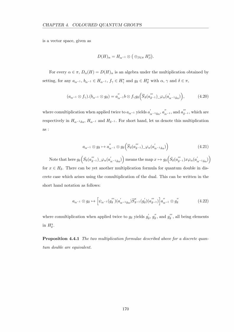
CHAPTER 4. COLOURED QUANTUM GROUPS
is a vector space, given as
D(H)α = Hα−1 ⊗(⊕β∈π H∗β
).
For every α ∈ π, Dα(H) = D(H)α is an algebra under the multiplication obtained by
setting, for any aα−1 , bα−1 ∈ Hα−1 , fγ ∈ H∗γ and gδ ∈ H∗δ with α, γ and δ ∈ π,
(aα−1 ⊗ fγ).(bα−1 ⊗ gδ) = a′′
α−1b⊗ fγgδ(Sδ(a
′′′
δ−1) ϕα(a′
α−1δα)), (4.20)
where comultiplication when applied twice to aα−1 yields a′
α−1δα, a′′
α−1 , and a′′′
δ−1 , which are
respectively in Hα−1δα, Hα−1 and Hδ−1 . For short hand, let us denote this multiplication
as :
aα−1 ⊗ gδ 7→ a′′
α−1 ⊗ gδ(Sδ(a
′′′
δ−1) ϕα(a′
α−1δα))
(4.21)
Note that here gδ
(Sδ(a
′′′
δ−1) ϕα(a′
α−1δα))
means the map x 7→ gδ
(Sδ(a
′′′
δ−1)xϕα(a′
α−1δα))
for x ∈ Hδ. There can be yet another multiplication formula for quantum double in dis-
crete case which arises using the comultiplication of the dual. This can be written in the
short hand notation as follows:
aα−1 ⊗ gδ 7→[ψα−1(g
′′′δ )(a
′
α−1δα)S∗δ−1(g
′δ)(a
′′′
δ−1)]a′′
α−1 ⊗ g′′δ (4.22)
where comultiplication when applied twice to gδ yields g′δ, g
′′δ , and g
′′′δ , all being elements
in H∗δ .
Proposition 4.4.1 The two multiplication formulae described above for a discrete quan-
tum double are equivalent.
170
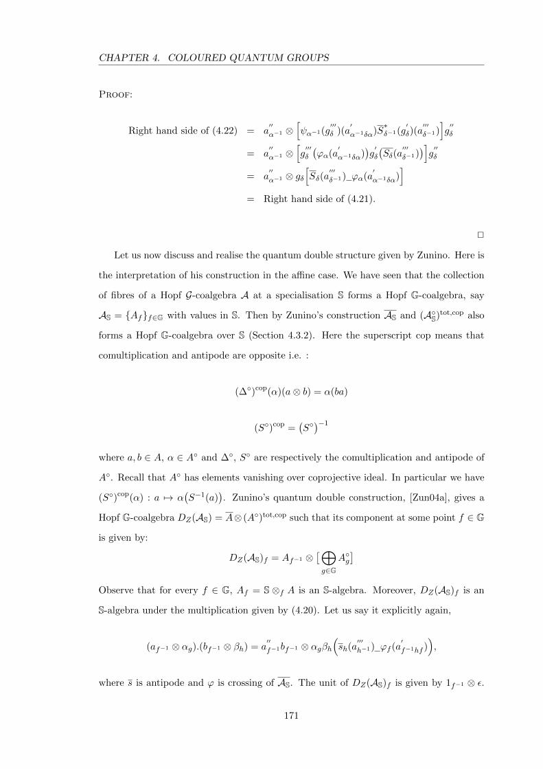
CHAPTER 4. COLOURED QUANTUM GROUPS
Proof:
Right hand side of (4.22) = a′′
α−1 ⊗[ψα−1(g
′′′δ )(a
′
α−1δα)S∗δ−1(g
′δ)(a
′′′
δ−1)]g′′δ
= a′′
α−1 ⊗[g′′′δ
(ϕα(a
′
α−1δα))g′δ
(Sδ(a
′′′
δ−1))]g′′δ
= a′′
α−1 ⊗ gδ[Sδ(a
′′′
δ−1) ϕα(a′
α−1δα)]
= Right hand side of (4.21).
2
Let us now discuss and realise the quantum double structure given by Zunino. Here is
the interpretation of his construction in the affine case. We have seen that the collection
of fibres of a Hopf G-coalgebra A at a specialisation S forms a Hopf G-coalgebra, say
AS = {Af}f∈G with values in S. Then by Zunino’s construction AS and (A◦S)tot,cop also
forms a Hopf G-coalgebra over S (Section 4.3.2). Here the superscript cop means that
comultiplication and antipode are opposite i.e. :
(∆◦)cop(α)(a⊗ b) = α(ba)
(S◦)cop =(S◦)−1
where a, b ∈ A, α ∈ A◦ and ∆◦, S◦ are respectively the comultiplication and antipode of
A◦. Recall that A◦ has elements vanishing over coprojective ideal. In particular we have
(S◦)cop(α) : a 7→ α(S−1(a)
). Zunino’s quantum double construction, [Zun04a], gives a
Hopf G-coalgebra DZ(AS) = A⊗ (A◦)tot,cop such that its component at some point f ∈ G
is given by:
DZ(AS)f = Af−1 ⊗[⊕g∈G
A◦g]
Observe that for every f ∈ G, Af = S ⊗f A is an S-algebra. Moreover, DZ(AS)f is an
S-algebra under the multiplication given by (4.20). Let us say it explicitly again,
(af−1 ⊗ αg).(bf−1 ⊗ βh) = a′′
f−1bf−1 ⊗ αgβh(sh(a
′′′
h−1) ϕf (a′
f−1hf )),
where s is antipode and ϕ is crossing of AS. The unit of DZ(AS)f is given by 1f−1 ⊗ ε.
171
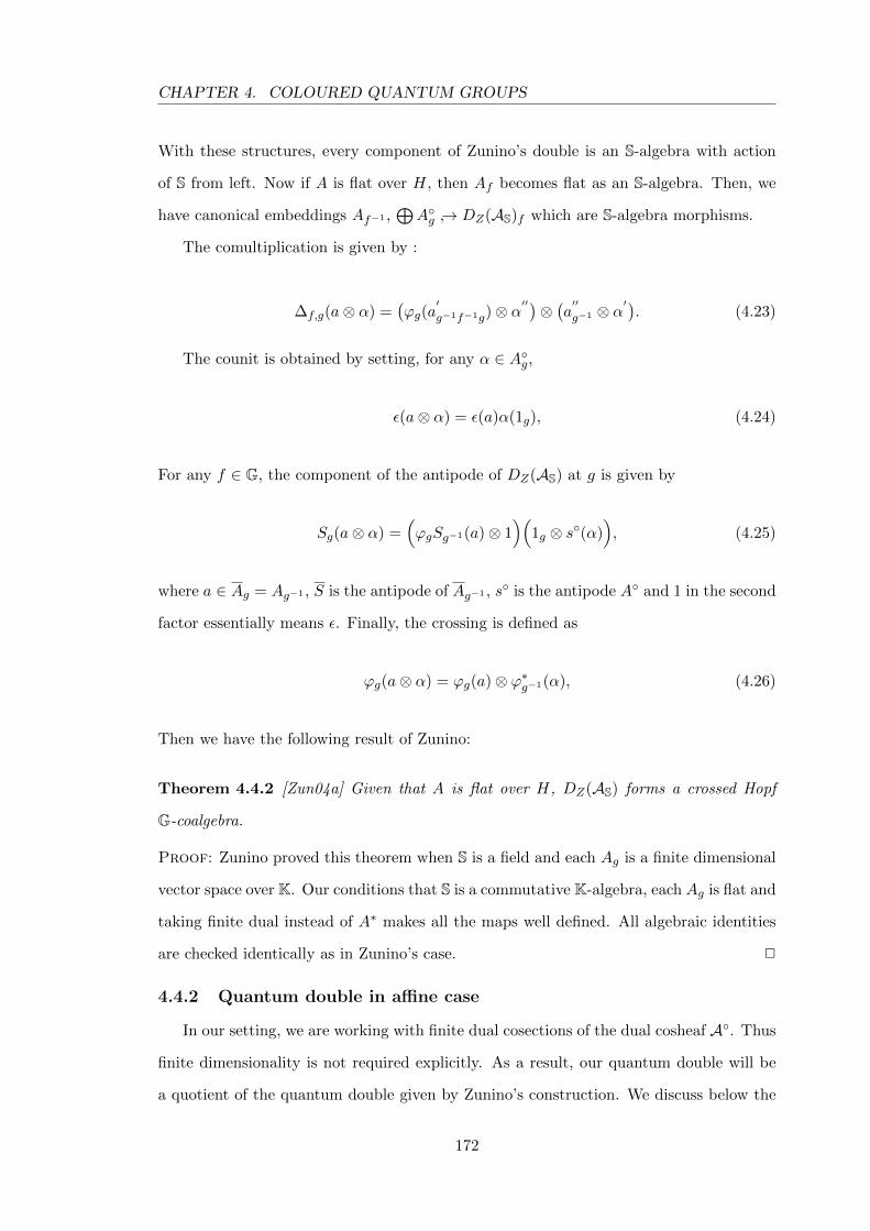
CHAPTER 4. COLOURED QUANTUM GROUPS
With these structures, every component of Zunino’s double is an S-algebra with action
of S from left. Now if A is flat over H, then Af becomes flat as an S-algebra. Then, we
have canonical embeddings Af−1 ,⊕A◦g ↪→ DZ(AS)f which are S-algebra morphisms.
The comultiplication is given by :
∆f,g(a⊗ α) =(ϕg(a
′
g−1f−1g)⊗ α′′)⊗ (a′′g−1 ⊗ α
′). (4.23)
The counit is obtained by setting, for any α ∈ A◦g,
ε(a⊗ α) = ε(a)α(1g), (4.24)
For any f ∈ G, the component of the antipode of DZ(AS) at g is given by
Sg(a⊗ α) =(ϕgSg−1(a)⊗ 1
)(1g ⊗ s◦(α)
), (4.25)
where a ∈ Ag = Ag−1 , S is the antipode of Ag−1 , s◦ is the antipode A◦ and 1 in the second
factor essentially means ε. Finally, the crossing is defined as
ϕg(a⊗ α) = ϕg(a)⊗ ϕ∗g−1(α), (4.26)
Then we have the following result of Zunino:
Theorem 4.4.2 [Zun04a] Given that A is flat over H, DZ(AS) forms a crossed Hopf
G-coalgebra.
Proof: Zunino proved this theorem when S is a field and each Ag is a finite dimensional
vector space over K. Our conditions that S is a commutative K-algebra, each Ag is flat and
taking finite dual instead of A∗ makes all the maps well defined. All algebraic identities
are checked identically as in Zunino’s case. 2
4.4.2 Quantum double in affine case
In our setting, we are working with finite dual cosections of the dual cosheaf A◦. Thus
finite dimensionality is not required explicitly. As a result, our quantum double will be
a quotient of the quantum double given by Zunino’s construction. We discuss below the
172
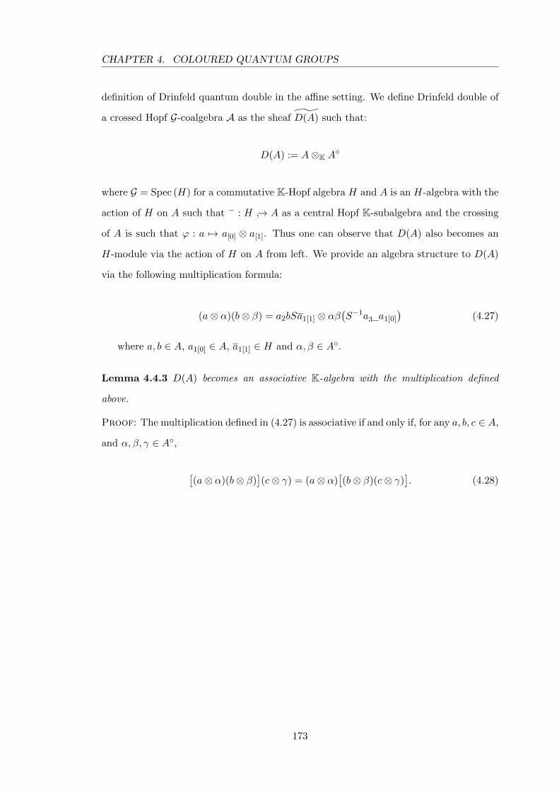
CHAPTER 4. COLOURED QUANTUM GROUPS
definition of Drinfeld quantum double in the affine setting. We define Drinfeld double of
a crossed Hopf G-coalgebra A as the sheaf D(A) such that:
D(A) := A⊗K A◦
where G = Spec (H) for a commutative K-Hopf algebra H and A is an H-algebra with the
action of H on A such that − : H ↪→ A as a central Hopf K-subalgebra and the crossing
of A is such that ϕ : a 7→ a[0] ⊗ a[1]. Thus one can observe that D(A) also becomes an
H-module via the action of H on A from left. We provide an algebra structure to D(A)
via the following multiplication formula:
(a⊗ α)(b⊗ β) = a2bSa1[1] ⊗ αβ(S−1a3 a1[0]
)(4.27)
where a, b ∈ A, a1[0] ∈ A, a1[1] ∈ H and α, β ∈ A◦.
Lemma 4.4.3 D(A) becomes an associative K-algebra with the multiplication defined
above.
Proof: The multiplication defined in (4.27) is associative if and only if, for any a, b, c ∈ A,
and α, β, γ ∈ A◦,
[(a⊗ α)(b⊗ β)
](c⊗ γ) = (a⊗ α)
[(b⊗ β)(c⊗ γ)
]. (4.28)
173
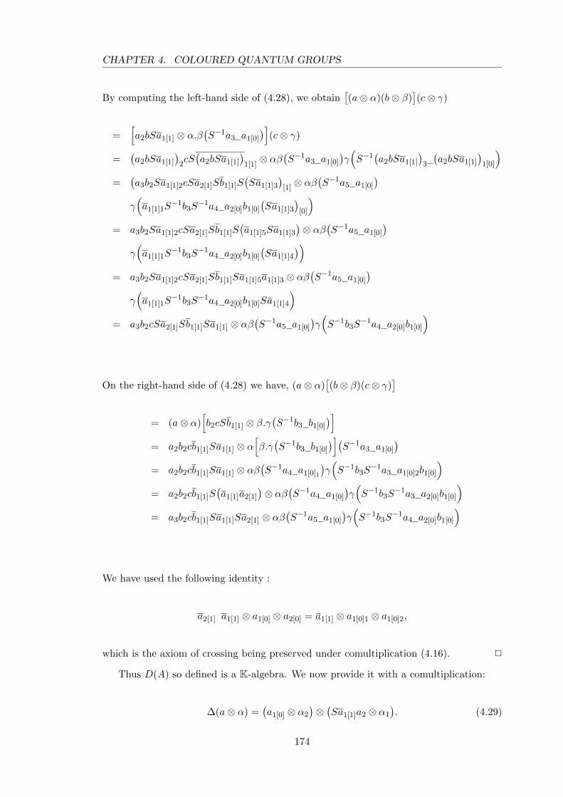
CHAPTER 4. COLOURED QUANTUM GROUPS
By computing the left-hand side of (4.28), we obtain[(a⊗ α)(b⊗ β)
](c⊗ γ)
=[a2bSa1[1] ⊗ α.β
(S−1a3 a1[0]
)](c⊗ γ)
=(a2bSa1[1]
)2cS(a2bSa1[1]
)1[1]⊗ αβ
(S−1a3 a1[0]
)γ(S−1
(a2bSa1[1]
)3
(a2bSa1[1]
)1[0]
)=
(a3b2Sa1[1]2cSa2[1]Sb1[1]S
(Sa1[1]3
)[1]⊗ αβ
(S−1a5 a1[0]
)γ(a1[1]1S
−1b3S−1a4 a2[0]b1[0]
(Sa1[1]3
)[0]
)= a3b2Sa1[1]2cSa2[1]Sb1[1]S
(a1[1]5Sa1[1]3
)⊗ αβ
(S−1a5 a1[0]
)γ(a1[1]1S
−1b3S−1a4 a2[0]b1[0]
(Sa1[1]4
))= a3b2Sa1[1]2cSa2[1]Sb1[1]Sa1[1]5a1[1]3 ⊗ αβ
(S−1a5 a1[0]
)γ(a1[1]1S
−1b3S−1a4 a2[0]b1[0]Sa1[1]4
)= a3b2cSa2[1]Sb1[1]Sa1[1] ⊗ αβ
(S−1a5 a1[0]
)γ(S−1b3S
−1a4 a2[0]b1[0]
)
On the right-hand side of (4.28) we have, (a⊗ α)[(b⊗ β)(c⊗ γ)
]= (a⊗ α)
[b2cSb1[1] ⊗ β.γ
(S−1b3 b1[0]
)]= a2b2cb1[1]Sa1[1] ⊗ α
[β.γ(S−1b3 b1[0]
)](S−1a3 a1[0]
)= a2b2cb1[1]Sa1[1] ⊗ αβ
(S−1a4 a1[0]1
)γ(S−1b3S
−1a3 a1[0]2b1[0]
)= a2b2cb1[1]S
(a1[1]a2[1]
)⊗ αβ
(S−1a4 a1[0]
)γ(S−1b3S
−1a3 a2[0]b1[0]
)= a3b2cb1[1]Sa1[1]Sa2[1] ⊗ αβ
(S−1a5 a1[0]
)γ(S−1b3S
−1a4 a2[0]b1[0]
)
We have used the following identity :
a2[1] a1[1] ⊗ a1[0] ⊗ a2[0] = a1[1] ⊗ a1[0]1 ⊗ a1[0]2,
which is the axiom of crossing being preserved under comultiplication (4.16). 2
Thus D(A) so defined is a K-algebra. We now provide it with a comultiplication:
∆(a⊗ α) =(a1[0] ⊗ α2
)⊗(Sa1[1]a2 ⊗ α1
). (4.29)
174
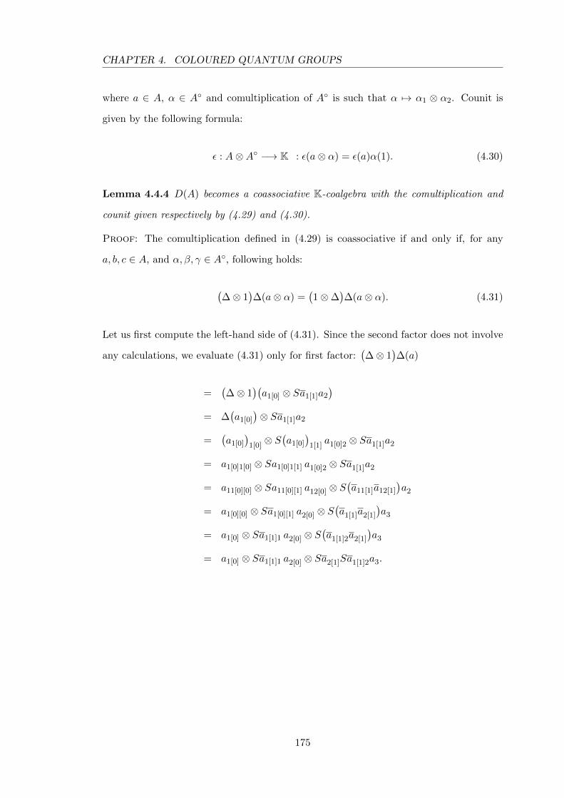
CHAPTER 4. COLOURED QUANTUM GROUPS
where a ∈ A, α ∈ A◦ and comultiplication of A◦ is such that α 7→ α1 ⊗ α2. Counit is
given by the following formula:
ε : A⊗A◦ −→ K : ε(a⊗ α) = ε(a)α(1). (4.30)
Lemma 4.4.4 D(A) becomes a coassociative K-coalgebra with the comultiplication and
counit given respectively by (4.29) and (4.30).
Proof: The comultiplication defined in (4.29) is coassociative if and only if, for any
a, b, c ∈ A, and α, β, γ ∈ A◦, following holds:
(∆⊗ 1
)∆(a⊗ α) =
(1⊗∆
)∆(a⊗ α). (4.31)
Let us first compute the left-hand side of (4.31). Since the second factor does not involve
any calculations, we evaluate (4.31) only for first factor:(∆⊗ 1
)∆(a)
=(∆⊗ 1
)(a1[0] ⊗ Sa1[1]a2
)= ∆
(a1[0]
)⊗ Sa1[1]a2
=(a1[0]
)1[0]⊗ S
(a1[0]
)1[1]
a1[0]2 ⊗ Sa1[1]a2
= a1[0]1[0] ⊗ Sa1[0]1[1] a1[0]2 ⊗ Sa1[1]a2
= a11[0][0] ⊗ Sa11[0][1] a12[0] ⊗ S(a11[1]a12[1]
)a2
= a1[0][0] ⊗ Sa1[0][1] a2[0] ⊗ S(a1[1]a2[1]
)a3
= a1[0] ⊗ Sa1[1]1 a2[0] ⊗ S(a1[1]2a2[1]
)a3
= a1[0] ⊗ Sa1[1]1 a2[0] ⊗ Sa2[1]Sa1[1]2a3.
175
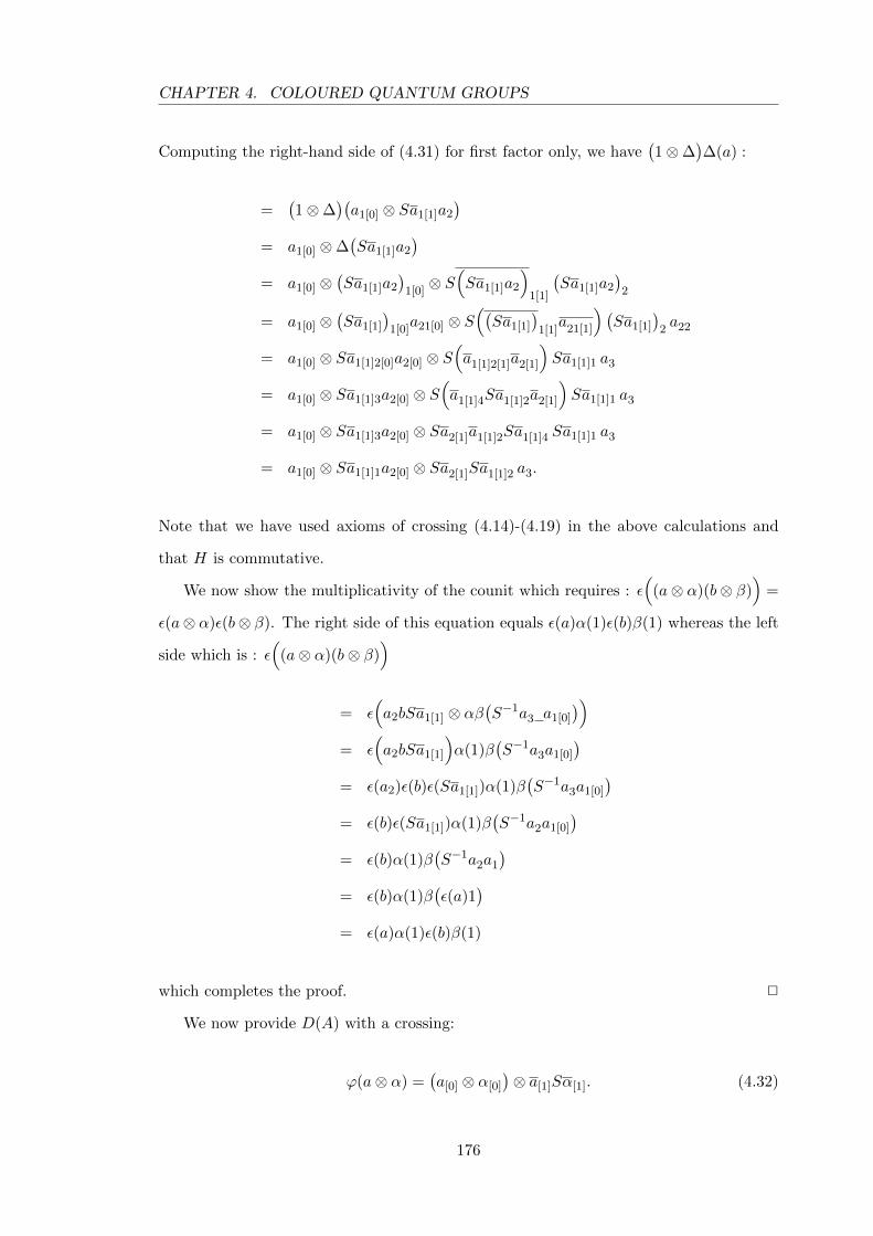
CHAPTER 4. COLOURED QUANTUM GROUPS
Computing the right-hand side of (4.31) for first factor only, we have(1⊗∆
)∆(a) :
=(1⊗∆
)(a1[0] ⊗ Sa1[1]a2
)= a1[0] ⊗∆
(Sa1[1]a2
)= a1[0] ⊗
(Sa1[1]a2
)1[0]⊗ S
(Sa1[1]a2
)1[1]
(Sa1[1]a2
)2
= a1[0] ⊗(Sa1[1]
)1[0]a21[0] ⊗ S
((Sa1[1]
)1[1]a21[1]
) (Sa1[1]
)2a22
= a1[0] ⊗ Sa1[1]2[0]a2[0] ⊗ S(a1[1]2[1]a2[1]
)Sa1[1]1 a3
= a1[0] ⊗ Sa1[1]3a2[0] ⊗ S(a1[1]4Sa1[1]2a2[1]
)Sa1[1]1 a3
= a1[0] ⊗ Sa1[1]3a2[0] ⊗ Sa2[1]a1[1]2Sa1[1]4 Sa1[1]1 a3
= a1[0] ⊗ Sa1[1]1a2[0] ⊗ Sa2[1]Sa1[1]2 a3.
Note that we have used axioms of crossing (4.14)-(4.19) in the above calculations and
that H is commutative.
We now show the multiplicativity of the counit which requires : ε(
(a⊗ α)(b⊗ β))
=
ε(a⊗ α)ε(b⊗ β). The right side of this equation equals ε(a)α(1)ε(b)β(1) whereas the left
side which is : ε(
(a⊗ α)(b⊗ β))
= ε(a2bSa1[1] ⊗ αβ
(S−1a3 a1[0]
))= ε
(a2bSa1[1]
)α(1)β
(S−1a3a1[0]
)= ε(a2)ε(b)ε(Sa1[1])α(1)β
(S−1a3a1[0]
)= ε(b)ε(Sa1[1])α(1)β
(S−1a2a1[0]
)= ε(b)α(1)β
(S−1a2a1
)= ε(b)α(1)β
(ε(a)1
)= ε(a)α(1)ε(b)β(1)
which completes the proof. 2
We now provide D(A) with a crossing:
ϕ(a⊗ α) =(a[0] ⊗ α[0]
)⊗ a[1]Sα[1]. (4.32)
176
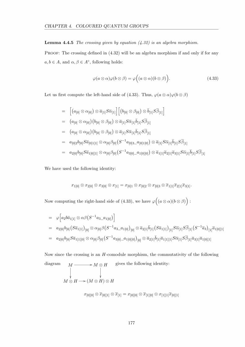
CHAPTER 4. COLOURED QUANTUM GROUPS
Lemma 4.4.5 The crossing given by equation (4.32) is an algebra morphism.
Proof: The crossing defined in (4.32) will be an algebra morphism if and only if for any
a, b ∈ A, and α, β ∈ A◦, following holds:
ϕ(a⊗ α)ϕ(b⊗ β) = ϕ(
(a⊗ α)(b⊗ β)). (4.33)
Let us first compute the left-hand side of (4.33). Thus, ϕ(a⊗ α)ϕ(b⊗ β)
=[(a[0] ⊗ α[0]
)⊗ a[1]Sα[1]
][(b[0] ⊗ β[0]
)⊗ b[1]Sβ[1]
]=
(a[0] ⊗ α[0]
)(b[0] ⊗ β[0]
)⊗ a[1]Sα[1]b[1]Sβ[1]
=(a[0] ⊗ α[0]
)(b[0] ⊗ β[0]
)⊗ a[1]Sα[1]b[1]Sβ[1]
= a[0]2b[0]Sa[0]1[1] ⊗ α[0]β[0]
(S−1a[0]3 a[0]1[0]
)⊗ a[1]Sα[1]b[1]Sβ[1]
= a2[0]b[0]Sa1[0][1] ⊗ α[0]β[0]
(S−1a3[0] a1[0][0]
)⊗ a1[1]a2[1]a3[1]Sα[1]b[1]Sβ[1]
We have used the following identity:
x1[0] ⊗ x2[0] ⊗ x3[0] ⊗ x[1] = x[0]1 ⊗ x[0]2 ⊗ x[0]3 ⊗ x1[1]x2[1]x3[1].
Now computing the right-hand side of (4.33), we have ϕ(
(a⊗ α)(b⊗ β))
:
= ϕ[a2ba1[1] ⊗ αβ
(S−1a3 a1[0]
)]= a2[0]b[0]
(Sa1[1]
)[0]⊗ α[0]β
(S−1a3 a1[0]
)[0]⊗ a2[1]b[1]
(Sa1[1]
)[1]Sα[1]Sβ[1]
(S−1a3
)[1]a1[0][1]
= a2[0]b[0]Sa1[1][0] ⊗ α[0]β[0]
(S−1a3[0] a1[0][0]
)[0]⊗ a2[1]b[1]a1[1][1]Sα[1]Sβ[1]a3[1]a1[0][1]
Now since the crossing is an H-comodule morphism, the commutativity of the following
diagram M //
��
M ⊗H
��M ⊗H // (M ⊗H)⊗H
gives the following identity:
x[0][0] ⊗ x[0][1] ⊗ x[1] = x[0][0] ⊗ x[1][0] ⊗ x[1][1]x[0][1]
177
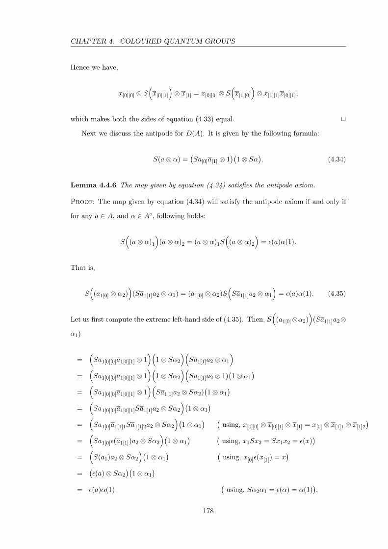
CHAPTER 4. COLOURED QUANTUM GROUPS
Hence we have,
x[0][0] ⊗ S(x[0][1]
)⊗ x[1] = x[0][0] ⊗ S
(x[1][0]
)⊗ x[1][1]x[0][1],
which makes both the sides of equation (4.33) equal. 2
Next we discuss the antipode for D(A). It is given by the following formula:
S(a⊗ α) =(Sa[0]a[1] ⊗ 1
)(1⊗ Sα
). (4.34)
Lemma 4.4.6 The map given by equation (4.34) satisfies the antipode axiom.
Proof: The map given by equation (4.34) will satisfy the antipode axiom if and only if
for any a ∈ A, and α ∈ A◦, following holds:
S(
(a⊗ α)1
)(a⊗ α)2 = (a⊗ α)1S
((a⊗ α)2
)= ε(a)α(1).
That is,
S(
(a1[0] ⊗ α2))
(Sa1[1]a2 ⊗ α1) = (a1[0] ⊗ α2)S(Sa1[1]a2 ⊗ α1
)= ε(a)α(1). (4.35)
Let us first compute the extreme left-hand side of (4.35). Then, S(
(a1[0]⊗α2))
(Sa1[1]a2⊗
α1)
=(Sa1[0][0]a1[0][1] ⊗ 1
)(1⊗ Sα2
)(Sa1[1]a2 ⊗ α1
)=
(Sa1[0][0]a1[0][1] ⊗ 1
)(1⊗ Sα2
)(Sa1[1]a2 ⊗ 1)
(1⊗ α1
)=
(Sa1[0][0]a1[0][1] ⊗ 1
)(Sa1[1]a2 ⊗ Sα2)
(1⊗ α1
)=
(Sa1[0][0]a1[0][1]Sa1[1]a2 ⊗ Sα2
)(1⊗ α1
)=
(Sa1[0]a1[1]1Sa1[1]2a2 ⊗ Sα2
)(1⊗ α1
) (using, x[0][0] ⊗ x[0][1] ⊗ x[1] = x[0] ⊗ x[1]1 ⊗ x[1]2
)=
(Sa1[0]ε(a1[1])a2 ⊗ Sα2
)(1⊗ α1
) (using, x1Sx2 = Sx1x2 = ε(x)
)=
(S(a1)a2 ⊗ Sα2
)(1⊗ α1
) (using, x[0]ε(x[1]) = x
)=
(ε(a)⊗ Sα2
)(1⊗ α1
)= ε(a)α(1)
(using, Sα2α1 = ε(α) = α(1)
).
178
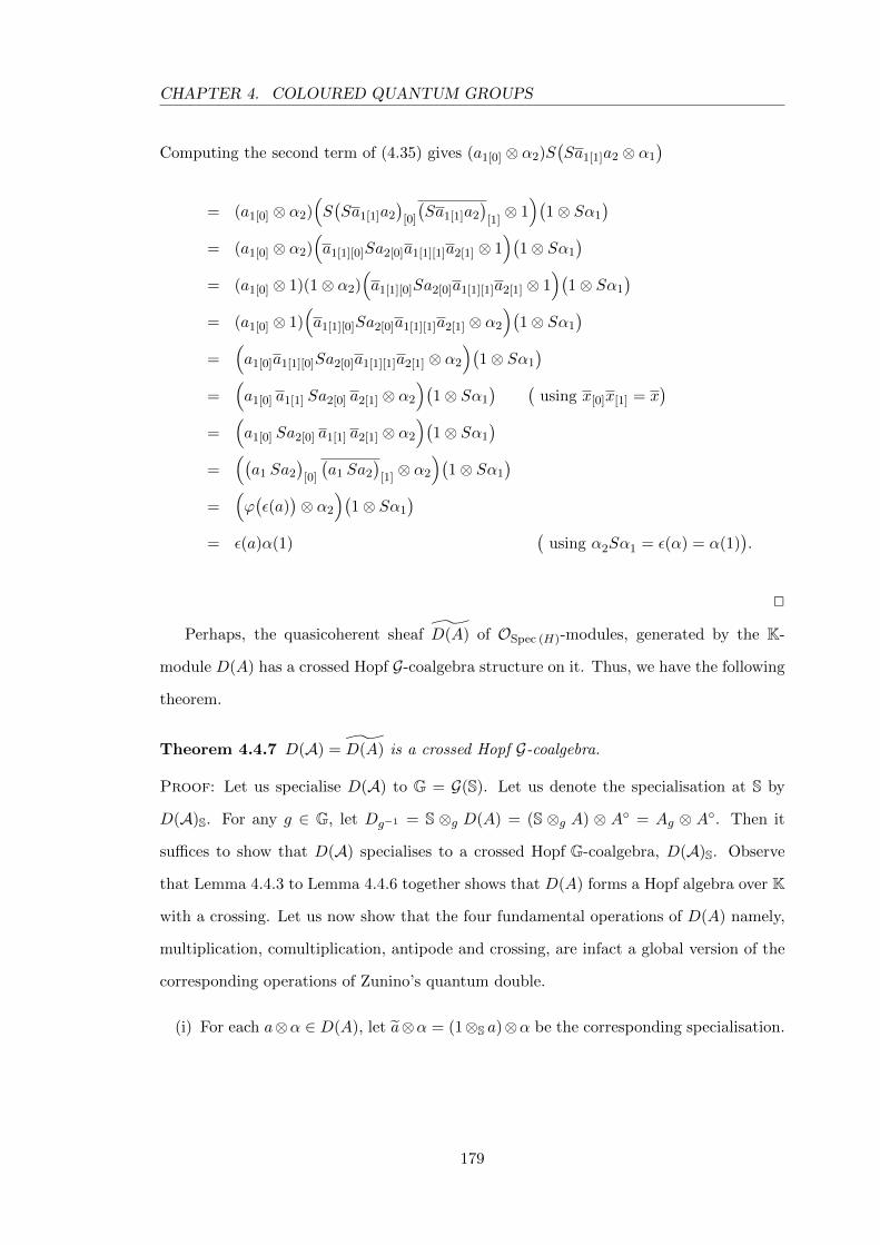
CHAPTER 4. COLOURED QUANTUM GROUPS
Computing the second term of (4.35) gives (a1[0] ⊗ α2)S(Sa1[1]a2 ⊗ α1
)= (a1[0] ⊗ α2)
(S(Sa1[1]a2
)[0]
(Sa1[1]a2
)[1]⊗ 1)(
1⊗ Sα1
)= (a1[0] ⊗ α2)
(a1[1][0]Sa2[0]a1[1][1]a2[1] ⊗ 1
)(1⊗ Sα1
)= (a1[0] ⊗ 1)(1⊗ α2)
(a1[1][0]Sa2[0]a1[1][1]a2[1] ⊗ 1
)(1⊗ Sα1
)= (a1[0] ⊗ 1)
(a1[1][0]Sa2[0]a1[1][1]a2[1] ⊗ α2
)(1⊗ Sα1
)=
(a1[0]a1[1][0]Sa2[0]a1[1][1]a2[1] ⊗ α2
)(1⊗ Sα1
)=
(a1[0] a1[1] Sa2[0] a2[1] ⊗ α2
)(1⊗ Sα1
) (using x[0]x[1] = x
)=
(a1[0] Sa2[0] a1[1] a2[1] ⊗ α2
)(1⊗ Sα1
)=
((a1 Sa2
)[0]
(a1 Sa2
)[1]⊗ α2
)(1⊗ Sα1
)=
(ϕ(ε(a)
)⊗ α2
)(1⊗ Sα1
)= ε(a)α(1)
(using α2Sα1 = ε(α) = α(1)
).
2
Perhaps, the quasicoherent sheaf D(A) of OSpec (H)-modules, generated by the K-
module D(A) has a crossed Hopf G-coalgebra structure on it. Thus, we have the following
theorem.
Theorem 4.4.7 D(A) = D(A) is a crossed Hopf G-coalgebra.
Proof: Let us specialise D(A) to G = G(S). Let us denote the specialisation at S by
D(A)S. For any g ∈ G, let Dg−1 = S ⊗g D(A) = (S ⊗g A) ⊗ A◦ = Ag ⊗ A◦. Then it
suffices to show that D(A) specialises to a crossed Hopf G-coalgebra, D(A)S. Observe
that Lemma 4.4.3 to Lemma 4.4.6 together shows that D(A) forms a Hopf algebra over K
with a crossing. Let us now show that the four fundamental operations of D(A) namely,
multiplication, comultiplication, antipode and crossing, are infact a global version of the
corresponding operations of Zunino’s quantum double.
(i) For each a⊗α ∈ D(A), let a⊗α = (1⊗S a)⊗α be the corresponding specialisation.
179
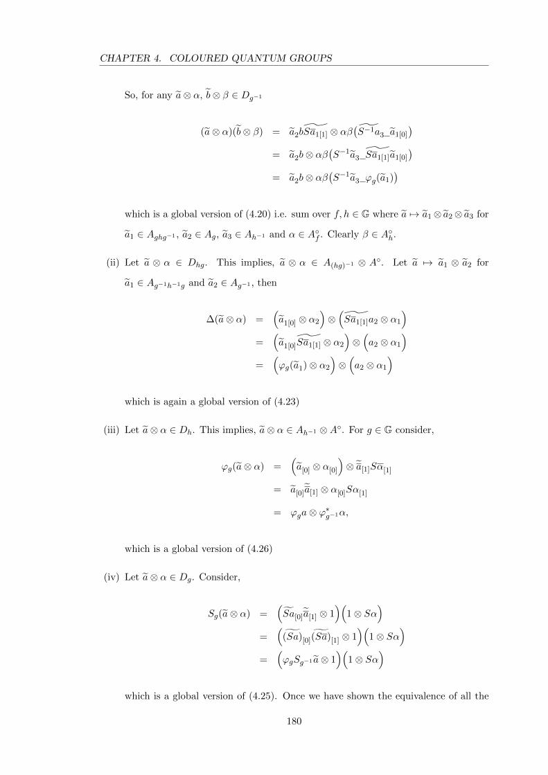
CHAPTER 4. COLOURED QUANTUM GROUPS
So, for any a⊗ α, b⊗ β ∈ Dg−1
(a⊗ α)(b⊗ β) = a2bSa1[1] ⊗ αβ(S−1a3 a1[0]
)= a2b⊗ αβ
(S−1a3 Sa1[1]a1[0]
)= a2b⊗ αβ
(S−1a3 ϕg(a1)
)which is a global version of (4.20) i.e. sum over f, h ∈ G where a 7→ a1⊗ a2⊗ a3 for
a1 ∈ Aghg−1 , a2 ∈ Ag, a3 ∈ Ah−1 and α ∈ A◦f . Clearly β ∈ A◦h.
(ii) Let a ⊗ α ∈ Dhg. This implies, a ⊗ α ∈ A(hg)−1 ⊗ A◦. Let a 7→ a1 ⊗ a2 for
a1 ∈ Ag−1h−1g and a2 ∈ Ag−1 , then
∆(a⊗ α) =(a1[0] ⊗ α2
)⊗(Sa1[1]a2 ⊗ α1
)=
(a1[0]Sa1[1] ⊗ α2
)⊗(a2 ⊗ α1
)=
(ϕg(a1)⊗ α2
)⊗(a2 ⊗ α1
)
which is again a global version of (4.23)
(iii) Let a⊗ α ∈ Dh. This implies, a⊗ α ∈ Ah−1 ⊗A◦. For g ∈ G consider,
ϕg(a⊗ α) =(a[0] ⊗ α[0]
)⊗ a[1]Sα[1]
= a[0]a[1] ⊗ α[0]Sα[1]
= ϕga⊗ ϕ∗g−1α,
which is a global version of (4.26)
(iv) Let a⊗ α ∈ Dg. Consider,
Sg(a⊗ α) =(Sa[0]a[1] ⊗ 1
)(1⊗ Sα
)=
((Sa)[0](Sa)[1] ⊗ 1
)(1⊗ Sα
)=
(ϕgSg−1 a⊗ 1
)(1⊗ Sα
)
which is a global version of (4.25). Once we have shown the equivalence of all the
180
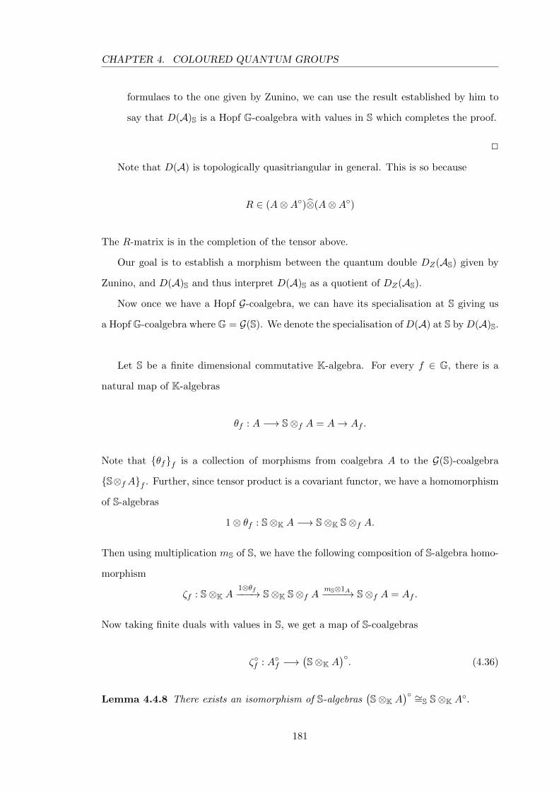
CHAPTER 4. COLOURED QUANTUM GROUPS
formulaes to the one given by Zunino, we can use the result established by him to
say that D(A)S is a Hopf G-coalgebra with values in S which completes the proof.
2
Note that D(A) is topologically quasitriangular in general. This is so because
R ∈ (A⊗A◦)⊗(A⊗A◦)
The R-matrix is in the completion of the tensor above.
Our goal is to establish a morphism between the quantum double DZ(AS) given by
Zunino, and D(A)S and thus interpret D(A)S as a quotient of DZ(AS).
Now once we have a Hopf G-coalgebra, we can have its specialisation at S giving us
a Hopf G-coalgebra where G = G(S). We denote the specialisation of D(A) at S by D(A)S.
Let S be a finite dimensional commutative K-algebra. For every f ∈ G, there is a
natural map of K-algebras
θf : A −→ S⊗f A = A→ Af .
Note that {θf}f is a collection of morphisms from coalgebra A to the G(S)-coalgebra
{S⊗f A}f . Further, since tensor product is a covariant functor, we have a homomorphism
of S-algebras
1⊗ θf : S⊗K A −→ S⊗K S⊗f A.
Then using multiplication mS of S, we have the following composition of S-algebra homo-
morphism
ζf : S⊗K A1⊗θf−−−→ S⊗K S⊗f A
mS⊗1A−−−−→ S⊗f A = Af .
Now taking finite duals with values in S, we get a map of S-coalgebras
ζ◦f : A◦f −→(S⊗K A
)◦. (4.36)
Lemma 4.4.8 There exists an isomorphism of S-algebras(S⊗K A
)◦ ∼=S S⊗K A◦.181
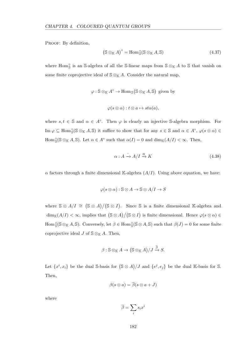
CHAPTER 4. COLOURED QUANTUM GROUPS
Proof: By definition, (S⊗K A
)◦= Hom ◦S(S⊗K A,S) (4.37)
where Hom ◦S is an S-algebra of all the S-linear maps from S ⊗K A to S that vanish on
some finite coprojective ideal of S⊗K A. Consider the natural map,
ϕ : S⊗K A◦ → Hom S(S⊗K A,S
)given by
ϕ(s⊗ α) : t⊗ a 7→ stα(a),
where s, t ∈ S and α ∈ A◦. Then ϕ is clearly an injective S-algebra morphism. For
Im ϕ ⊆ Hom ◦S(S ⊗K A,S) it suffice to show that for any s ∈ S and α ∈ A◦, ϕ(s ⊗ α) ∈
Hom ◦S(S⊗K A,S). Let α ∈ A◦ such that α(I) = 0 and dimK(A/I) <∞. Then,
α : A−−→ A/I
α−→ K (4.38)
α factors through a finite dimensional K-algebra (A/I). Using above equation, we have:
ϕ(s⊗ α) : S⊗A→ S⊗A/I → S
where S ⊗ A/I ∼=(S ⊗ A
)/(S ⊗ I
). Since S is a finite dimensional K-algebra and
dimK(A/I) < ∞, implies that(S ⊗ A
)/(S ⊗ I
)is finite dimensional. Hence ϕ(s ⊗ α) ∈
Hom ◦S(S⊗K A,S). Conversely, let β ∈ Hom ◦S(S⊗A, S) such that β(J) = 0 for some finite
coprojective ideal J of S⊗K A. Then,
β : S⊗K A→(S⊗K A
)/J
β−→ S.
Let {xi, xi} be the dual S-basis for(S ⊗ A
)/J and {ej , ej} be the dual K-basis for S.
Then,
β(s⊗ a) = β(s⊗ a+ J)
where
β =∑i
sixi
182
CHAPTER 4. COLOURED QUANTUM GROUPS
for si ∈ S. Let
xi : S⊗K A→(S⊗K A
)/J
xi−→ S.
Then observe that
β = ϕ(∑i,j
siej ⊗ ej xi).
Indeed,
ϕ(∑i,j
siej ⊗ ej xi)(t⊗ a) =
∑i,j
tsiejej(xi(a))
=∑i
tsi(xi(a))
= tβ(a)
= β(t⊗ a)
Thus, β ∈ Im ϕ, which completes the proof. 2
Let Γ =(A◦)tot,cop
=⊕
f∈GA◦f . Then by definition of ( )tot (defined by Zunino), it
has a Hopf algebra structure. Here Γ has a S-Hopf algebra structure as each of the fibre
A◦f is an S-coalgebra. If ϕ : A → A ⊗ H is the crossing of A and ϕ◦ : A◦ → A◦ ⊗ H is
the crossing of A◦, then the crossing of Γ is simply the sum of the crossings of each of the
fiber Af . Let us denote it as ϕΓ which is an S-algebra morphism from Γ to Γ⊗H. Also,
1⊗ ϕ◦ : S⊗K A◦ −→ S⊗K A◦ ⊗H gives a crossing of S⊗K A◦.
Now using the canonical projection π :⊕
f∈GA◦f −→ A◦f , for f ∈ G along with the
above lemma and equation (4.36), we get the following map of S-coalgebras:
π : Γ −→ S⊗K A◦
where π = ζ◦f π such that, π(αf ) : 1 ⊗S a 7→ αf (a), αf ∈ A◦f for some f ∈ G and a ∈ A.
Note that the way π is defined, it preserves the crossing of the two S-Hopf algebras Γ and
S⊗K A◦, ı.e.
(1⊗ ϕ◦)π = (π ⊗ 1)ϕΓ. (4.39)
Note that Ag−1 is flat as an S-algebra for any g ∈ G. Thus for each g ∈ G, we have
183
CHAPTER 4. COLOURED QUANTUM GROUPS
following composition of maps:
φg−1 : Ag−1 ⊗ Γ1⊗π−−→ Ag−1 ⊗ S⊗A◦ −→ Ag−1 ⊗A◦.
Let us denote the collection of these maps by Φ = {φg−1}g∈G. So far Φ is a collection of
linear maps. We claim that this will be indeed a crossed Hopf group coalgebra morphism
between the global sections of the two quantum doubles. Thus we have our main theorem
of the chapter:
Theorem 4.4.9 Let G = Spec (H) be an affine group scheme, A be a coherent, locally free
crossed Hopf G-coalgebra over G, and S be a finite dimensional commutative K-algebra.
Then Φ is a morphism of crossed Hopf G(S)-coalgebra from Zunino’s quantum double
DZ(AS) to D(A)S.
Proof: For each g ∈ G,
φg : Ag ⊗(⊕f∈G
Af◦) −→ Ag ⊗A◦,
where Φ = {φg−1}g∈G. Now Φ is a crossed Hopf G(S)-coalgebra morphism if and only if
it is compatible with respect to the four fundamental structures, namely multiplication,
comultiplication, counit and crossing. Compatibility with respect to unit and antipode
would follow automatically. Observe that
Φ(1⊗ α)(1⊗ β) = Φ(1⊗ α)Φ(1⊗ β)
because π is an algebra map which is true since θf intertwines coalgebra structure on A
with G(S)-coalgebra structure on {Af}f , that is,
∆f,g ◦ θfg = (θf ⊗ θg) ◦∆.
Moreover, each φf preserves multiplication. Note that on more general elements in
DZ(AS), (ag ⊗αf )(bg ⊗ βh) = (a′′gbg ⊗
∑f,h αfβh
(Sh(a
′′′
h−1) ϕg−1(a′
ghg−1))
where ag, bg ∈
184
CHAPTER 4. COLOURED QUANTUM GROUPS
Ag, αf ∈ A◦f , βh ∈ A◦h. Thus we have φg
[(ag ⊗ αf )(bg ⊗ βh)
]
= φg
[(a′′gbg ⊗ αfβh
(Sh(a
′′′
h−1) ϕg−1(a′
ghg−1))]
= a′′gbg ⊗ π
[αfβh
(Sh(a
′′′
h−1) ϕg−1(a′
ghg−1))]
= a′′gbg ⊗ παfπ
[βh
(S−1h (a
′′′
h−1) ϕg−1(a′
ghg−1))] (
because π is an algebra morphism)
= a′′gbg ⊗ παfπβh
(S−1h (a
′′′
h−1) ϕg−1(a′
ghg−1)) (
because π is a coalgebra morphism.)
where ag 7→ a′
ghg−1 ⊗ a′′g ⊗ a
′′′
h−1 . Compare it with the multiplication of φg[(ag ⊗ αf )
]and
φg[(bg ⊗ βh)
]in D(A)S. In the latter case we use Theorem (4.4.7) and we have:
=[ag ⊗ παf
][bg ⊗ πβh
]= a
′′gbg ⊗ παfπβh
(S−1(a
′′′
h−1) ϕg−1(a′
ghg−1)).
Thus multiplication is preserved under Φ. Similarly we can show that Φ preserves the
other operations. Calculations are quite similar as above or as we have done in Theorem
4.4.7. In this way, Φ becomes indeed a morphism of crossed Hopf G-coalgebra. This
completes the proof.
2
Observe that in case the maps θf are injections, then π in turn becomes a surjection,
making each of φf a surjection. In such a case D(A)S becomes a quotient of Zunino’s
quantum double DZ(AS).
Example. Quantum double in affine case.
Assume that 0 6= q ∈ K and that q is not a root of unity. Let A be the coordinate ring
of quantum 2× 2 matrices, which is defined to be A = Oq(M2(K)
)= K〈a, b, c, d〉 subject
to the relations
ba = q−2ab ca = q−2ac bc = cb
db = q−2bd dc = q−2cd ad− da = (q2 − q−2)bc
Then A becomes a bialgebra by the following setting. If we write
185
CHAPTER 4. COLOURED QUANTUM GROUPS
X =
a b
c d
=
X11 X12
X21 X22
, (4.40)
the coproduct and counit are given by ∆(Xij) =∑
kXik⊗Xkj , and ε(Xij) = δij . Let the
quantum determinant be detqX = ad − q2bc. Let A be the quantum SL2(K) is defined
as
Oq(SL2(K)) = Oq(M2(K))/(detqX − 1).
It inherits a bialgebra structure from Oq(M2(K)). Indeed, it forms a Hopf algebra struc-
ture with the antipode map given as
S
a b
c d
= (ad− q2bc)−1
d −q−2b
−q2c a
That is, Sa = (ad−q2bc)−1d, etc. Now let B be the q-analogue of the universal enveloping
algebra of the classical Lie algebra g = sl(2). Let us recall the definition.
B = Uq(sl(2)
)= K〈E,F,K,K−1〉
with the relations KE = q2EK, KF = q−2FK and EF − FE =K2 −K−2
(q2 − q−2). There is a
Hopf algebra structure on B defined by
∆(E) = E ⊗K−1 +K ⊗ E, S(E) = −q−2E, ε(E) = 0
∆(F ) = F ⊗K−1 +K ⊗ F, S(F ) = −q2F, ε(F ) = 0
∆(K) = K ⊗K, S(K) = K−1, ε(K) = 1
Both ∆ and ε extend to algebra homomorphisms, and S extends to an algebra anti-
homomorphism.
Let us provide a pairing σ : A ⊗ B → K between the two Hopf algebras A and B
186
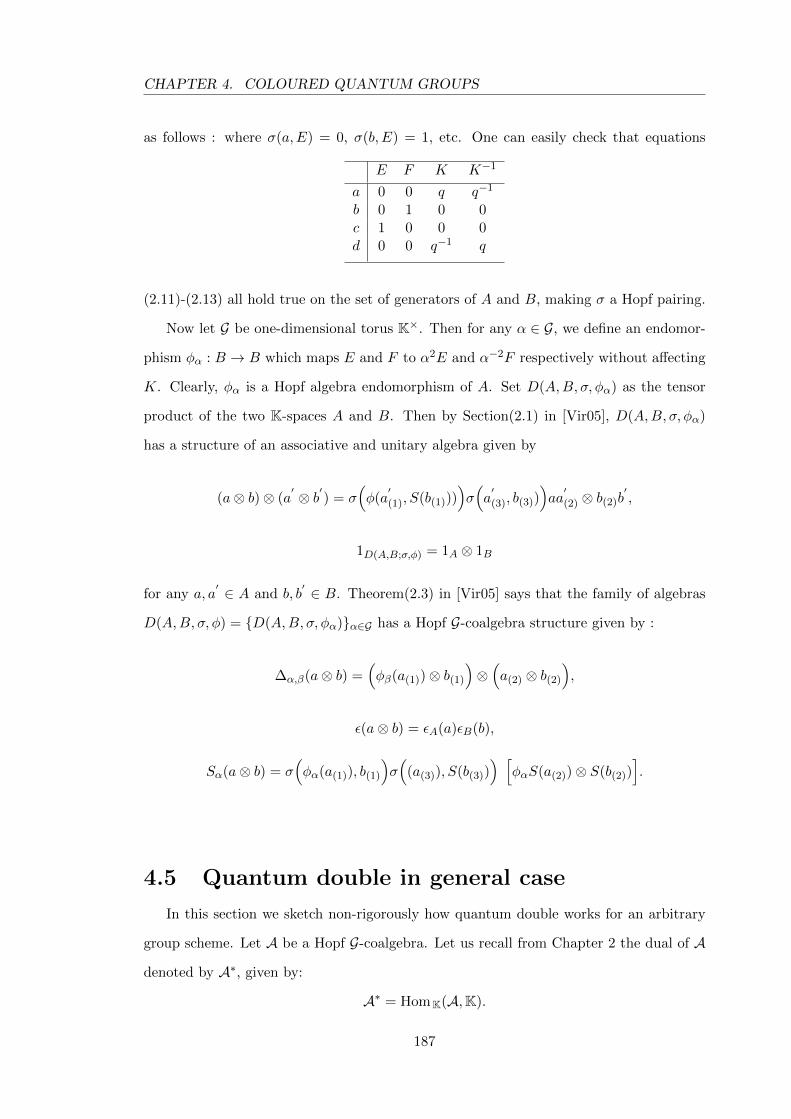
CHAPTER 4. COLOURED QUANTUM GROUPS
as follows : where σ(a,E) = 0, σ(b, E) = 1, etc. One can easily check that equations
E F K K−1
a 0 0 q q−1
b 0 1 0 0c 1 0 0 0d 0 0 q−1 q
(2.11)-(2.13) all hold true on the set of generators of A and B, making σ a Hopf pairing.
Now let G be one-dimensional torus K×. Then for any α ∈ G, we define an endomor-
phism φα : B → B which maps E and F to α2E and α−2F respectively without affecting
K. Clearly, φα is a Hopf algebra endomorphism of A. Set D(A,B, σ, φα) as the tensor
product of the two K-spaces A and B. Then by Section(2.1) in [Vir05], D(A,B, σ, φα)
has a structure of an associative and unitary algebra given by
(a⊗ b)⊗ (a′ ⊗ b′) = σ
(φ(a
′
(1), S(b(1))))σ(a′
(3), b(3)))aa′
(2) ⊗ b(2)b′,
1D(A,B;σ,φ) = 1A ⊗ 1B
for any a, a′ ∈ A and b, b
′ ∈ B. Theorem(2.3) in [Vir05] says that the family of algebras
D(A,B, σ, φ) = {D(A,B, σ, φα)}α∈G has a Hopf G-coalgebra structure given by :
∆α,β(a⊗ b) =(φβ(a(1))⊗ b(1)
)⊗(a(2) ⊗ b(2)
),
ε(a⊗ b) = εA(a)εB(b),
Sα(a⊗ b) = σ(φα(a(1)), b(1)
)σ(
(a(3)), S(b(3))) [
φαS(a(2))⊗ S(b(2))].
4.5 Quantum double in general case
In this section we sketch non-rigorously how quantum double works for an arbitrary
group scheme. Let A be a Hopf G-coalgebra. Let us recall from Chapter 2 the dual of A
denoted by A∗, given by:
A∗ = HomK(A,K).
187
CHAPTER 4. COLOURED QUANTUM GROUPS
Then for each open covering {Ui} of U ⊆ G, the sheaf exact sequence of K-modules,
∏i,j
A(Ui ∩ Uj)⇔∏i
A(Ui)←− A(U)←− 0
turns into cosheaf exact sequence of K-modules
⊕i,jA∗(Ui ∩ Uj)⇒ ⊕iA∗(Ui) −→ A∗(U) −→ 0.
Thus A∗ is a cosheaf of K-modules over group scheme G. Now let us recall from chapter
2 the finite dual of A. From (2.10), we have
A◦ ={f ∈ A∗
∣∣∣f(I) = 0 for some ideal I of A ; dimKA/I <∞
}.
Equivalently, we can say that A◦ has those elements of A∗ which vanish on some finite
coprojective ideal of A. Cosections of A◦ are subspaces of the corresponding cosections
of A∗. Indeed they are coalgebras over K, (cf. (2.16)). For each inclusion of open sets
U ⊆ V , the corestriction cores◦V,U : A◦(U)→ A◦(V ) is given by the following sequence
cores◦V,U (f) : A(V )resU,V−−−−→ A(U) −→ fM −→ K,
Thus the corestrictions of the cosheaf A◦ are induced by the restrictions of A∗. This
makes A◦ a subcosheaf of A∗.
Note that µ∗(A � A)(G) 6= A(G) ⊗ A(G). Infact, A(G) ⊗ A(G) sits naturally inside
µ∗(A�A)(G). Consider the following example:
Example. Let G be a discrete infinite group. Let A be the constant sheaf over G with
fibre at each point to be the ground field K. Comultiplication on A is simply the identity
map ∆g,h : Ag,h → Ag⊗KAh as Agh = K, and Ag⊗Ah = K⊗K = K. A(G) =∏g∈G Ag =∏
g∈G Kg. The global section is the infinite product over G of the copies of K. If x ∈ A(G),
then clearly, ∆x ∈∏g,h∈G(Ag ⊗Ah) but
∏g∈G Ag ⊗
∏h∈G Ah
∏g,h∈G(Ag ⊗Ah). Now
the dual cosheaf is given as A(G)◦ = {∑n
i=i αiπgi |αi ∈ K}; πg : A(G) → A(G). Then
A◦(G) is isomorphic to the group algebra, KG (cf. Theorem 4.5.3).
188
CHAPTER 4. COLOURED QUANTUM GROUPS
Next we discuss the global section of A. Let
Γ = Γ(G,A) = A(G).
Let us recall the result we proved in Chapter 2, Lemma (2.6.1):
Lemma 4.5.1 Suppose A is a sheaf of algebras over a group scheme G. If A is generated
by global sections Γ, then A�A is generated by Γ× Γ.
This helps us to formulate the following conjecture:
Conjecture 4.5.2 Let U ⊆ G be an open subset such that µ−1(U) ⊆ π−11 (U) ∩ π−1
2 (U)
and Im e ⊆ U . Let A be finitely generated by global sections. Then A◦(U) is an associative
algebra with identity.
In particular, the global cosection of the dual cosheaf A◦(G) is an associative algebra
with identity. In fact a bigger statement is true which is stated in the form of a theorem
below. We do not prove the theorem as this section is mainly speculative, and it uses the
above conjecture.
Conjecture 4.5.3 Suppose A is a Hopf G-coalgebra generated by global sections. Then
A◦(G) is a Hopf algebra over K in the usual sense of a vector space.
The above theorem is crucial as it assists in framing the structure of a quantum double
in the general case.
Conjecture 4.5.4 Suppose A is a crossed Hopf G-coalgebra generated by global sections.
Then D(A) := A⊗ Γ is a quasitriangular crossed Hopf G-coalgebra, where Γ = A◦(G).
The structures of D(A) are consistent with Theorem (4.4.7). Further, if A is not
generated by global sections, it should be a tensor product of a sheaf A and its dual
cosheaf A◦ which will be studied by the mathematicians of future generations.
189
Bibliography
[AEHDVD07] A. T. Abd El-Hafez, L. Delvaux, and A. Van Daele. Group-cograded
multiplier Hopf (∗-)algebras. Algebr. Represent. Theory, 10(1):77–95, 2007.
[AM02] A.T. Abd El-hafez A.S.Hegazi and M.Mansour. Multiplier Hopf group
coalgebra. 2002.
[Ati88] Michael Atiyah. Topological quantum field theories. Inst. Hautes Etudes
Sci. Publ. Math., (68):175–186 (1989), 1988.
[Bre97] Glen E. Bredon. Sheaf theory, volume 170 of Graduate Texts in Mathe-
matics. Springer-Verlag, New York, second edition, 1997.
[Brz00] Tomasz Brzezinski. Frobenius properties and Maschke-type theorems for
entwined modules. Proc. Amer. Math. Soc., 128(8):2261–2270, 2000.
[Brz09] Tomasz Brzezinski. Comodules and corings. In Handbook of algebra. Vol.
6, volume 6 of Handb. Algebr., pages 237–318. Elsevier/North-Holland,
Amsterdam, 2009.
[BT00] Mark Brightwell and Paul Turner. Representations of the homotopy sur-
face category of a simply connected space. J. Knot Theory Ramifications,
9(7):855–864, 2000.
[BT03] Mark Brightwell and Paul Turner. Modular functors in homotopy quantum
field theory and tortile structures. J. Pure Appl. Algebra, 185(1-3):43–71,
2003.
190
BIBLIOGRAPHY
[BTW02] U. Bunke, P. Turner, and S. Willerton. Gerbes and homotopy quantum
field theories. ArXiv Mathematics e-prints, January 2002.
[BTW03] Mark Brightwell, Paul Turner, and Simon Willerton. Homotopy quantum
field theories and related ideas. In Proceedings of the Tenth Oporto Meeting
on Geometry, Topology and Physics (2001), volume 18, pages 115–122,
2003.
[BTW04] Ulrich Bunke, Paul Turner, and Simon Willerton. Gerbes and homotopy
quantum field theories. Algebr. Geom. Topol., 4:407–437, 2004.
[BW99] John W. Barrett and Bruce W. Westbury. Spherical categories. Adv.
Math., 143(2):357–375, 1999.
[BW05] Michael Barr and Charles Wells. Toposes, triples and theories. Repr.
Theory Appl. Categ., (12):x+288, 2005. Corrected reprint of the 1985
original [MR0771116].
[CD05] E. Castillo and R. Diaz. Homological Quantum Field Theory. ArXiv
Mathematics e-prints, September 2005.
[CG97] Neil Chriss and Victor Ginzburg. Representation theory and complex ge-
ometry. Birkhauser Boston Inc., Boston, MA, 1997.
[CMZ02] Stefaan Caenepeel, Gigel Militaru, and Shenglin Zhu. Frobenius and sep-
arable functors for generalized module categories and nonlinear equations,
volume 1787 of Lecture Notes in Mathematics. Springer-Verlag, Berlin,
2002.
[Del08] L. Delvaux. Yetter-Drinfel′d modules for group-cograded multiplier Hopf
algebras. Comm. Algebra, 36(8):2872–2882, 2008.
[Dri85] V. G. Drinfeld. Hopf algebras and the quantum Yang-Baxter equation.
Dokl. Akad. Nauk SSSR, 283(5):1060–1064, 1985.
191
BIBLIOGRAPHY
[Dri87] V. G. Drinfeld. Quantum groups. In Proceedings of the International
Congress of Mathematicians, Vol. 1, 2 (Berkeley, Calif., 1986), pages 798–
820, Providence, RI, 1987. Amer. Math. Soc.
[DVD07] Lydia Delvaux and Alfons Van Daele. The Drinfel′d double for group-
cograded multiplier Hopf algebras. Algebr. Represent. Theory, 10(3):197–
221, 2007.
[DvDW05] L. Delvaux, A. van Daele, and S. H. Wang. Quasitriangular (G-cograded)
multiplier Hopf algebras. J. Algebra, 289(2):484–514, 2005.
[Eil52] Samuel Eilenberg. Homotopy groups and algebraic homology theories. In
Proceedings of the International Congress of Mathematicians, Cambridge,
Mass., 1950, vol. 2, pages 350–353, Providence, R. I., 1952. Amer. Math.
Soc.
[EM53] Samuel Eilenberg and Saunders MacLane. On the groups of H(Π, n). I.
Ann. of Math. (2), 58:55–106, 1953.
[FY89] Peter J. Freyd and David N. Yetter. Braided compact closed categories
with applications to low-dimensional topology. Adv. Math., 77(2):156–182,
1989.
[GTMW09] Søren Galatius, Ulrike Tillmann, Ib Madsen, and Michael Weiss. The
homotopy type of the cobordism category. Acta Math., 202(2):195–239,
2009.
[Har77] Robin Hartshorne. Algebraic geometry. Springer-Verlag, New York, 1977.
Graduate Texts in Mathematics, No. 52.
[HIE08] A. S. Hegazi, F. Ismail, and M. M. Elsofy. Induced and coinduced represen-
tations of Hopf group coalgebras. Appl. Categ. Structures, 16(1-2):97–102,
2008.
[HT80] A. Hatcher and W. Thurston. A presentation for the mapping class group
of a closed orientable surface. Topology, 19(3):221–237, 1980.
192
BIBLIOGRAPHY
[Jim85] Michio Jimbo. A q-difference analogue of U(g) and the Yang-Baxter equa-
tion. Lett. Math. Phys., 10(1):63–69, 1985.
[JS91] Andr’e Joyal and Ross Street. The geometry of tensor calculus. I. Adv.
Math., 88(1):55–112, 1991.
[JS93] Andr’e Joyal and Ross Street. Braided tensor categories. Advances in
Mathematics, 102(1):20 – 78, 1993.
[Kho00] Mikhail Khovanov. A categorification of the Jones polynomial. Duke Math.
J., 101(3):359–426, 2000.
[KL80] G. M. Kelly and M. L. Laplaza. Coherence for compact closed categories.
J. Pure Appl. Algebra, 19:193–213, 1980.
[Lee05] Eun Soo Lee. An endomorphism of the Khovanov invariant. Adv. Math.,
197(2):554–586, 2005.
[Mac52] Saunders MacLane. Cohomology theory of Abelian groups. In Proceedings
of the International Congress of Mathematicians, Cambridge, Mass., 1950,
vol. 2, pages 8–14, Providence, R. I., 1952. Amer. Math. Soc.
[Mac63] Saunders MacLane. Natural associativity and commutativity. Rice Univ.
Studies, 49(4):28–46, 1963.
[ML98] Saunders Mac Lane. Categories for the working mathematician, volume 5
of Graduate Texts in Mathematics. Springer-Verlag, New York, second
edition, 1998.
[Mug05] Michael Muger. Erratum: “Conformal orbifold theories and braided
crossed G-categories” [Comm. Math. Phys. 260 (2005), no. 3, 727–762;
2183964]. Comm. Math. Phys., 260(3):763, 2005.
[Oht93] Tomotada Ohtsuki. Colored ribbon Hopf algebras and universal invariants
of framed links. J. Knot Theory Ramifications, 2(2):211–232, 1993.
193
BIBLIOGRAPHY
[PS07] Florin Panaite and Mihai D. Staic. Generalized (anti) Yetter-Drinfeld
modules as components of a braided T -category. Israel J. Math., 158:349–
365, 2007.
[PT08] Timothy Porter and V. Turaev. Formal homotopy quantum field theo-
ries. I. Formal maps and crossed C-algebras. J. Homotopy Relat. Struct.,
3(1):113–159, 2008.
[Qui95] Frank Quinn. Lectures on axiomatic topological quantum field theory. In
Geometry and quantum field theory (Park City, UT, 1991), volume 1 of
IAS/Park City Math. Ser., pages 323–453. Amer. Math. Soc., Providence,
RI, 1995.
[Rod01] G. Rodrigues. Homotopy Quantum Field Theories and the Homotopy
Cobordism Category in Dimension 1+1. ArXiv Mathematics e-prints, May
2001.
[Rod03] Goncalo Rodrigues. Homotopy quantum field theories and the homotopy
cobordism category in dimension 1 + 1. J. Knot Theory Ramifications,
12(3):287–319, 2003.
[RT90] N. Yu. Reshetikhin and V. Turaev. Ribbon graphs and their invariants
derived from quantum groups. Comm. Math. Phys., 127(1):1–26, 1990.
[S.C04] M.Delombaerde S.Caenepeel. A categorical approach to Turaev Hopf
group- coalgebras. 2004.
[Shu94] Mei Chee Shum. Tortile tensor categories. J. Pure Appl. Algebra, 93(1):57–
110, 1994.
[Spa81] Edwin H. Spanier. Algebraic topology. Springer-Verlag, New York, 1981.
Corrected reprint.
[ST09] M. D. Staic and V. Turaev. Remarks on 2-dimensional HQFT’s. 2009.
[Tur99] V. Turaev. Homotopy field theory in dimension 2 and group-algebras.
1999.
194
BIBLIOGRAPHY
[Tur00] V. Turaev. Homotopy field theory in dimension 3 and crossed group-
categories. 2000.
[Tur08] V. Turaev. Crossed group-categories. Arab. J. Sci. Eng. Sect. C Theme
Issues, 33(2):483–503, 2008.
[Tur10a] V. Turaev. Homotopy quantum field theory / Vladimir Turaev ; with ap-
pendices by Michael Muger and Alexis Virelizier, volume 59 of EMS Tracts
in mathematics ; 10. Zrich : European Mathematical Society Publishing
House, cop. 2010, Cambridge, 2010.
[Tur10b] Vladimir G. Turaev. Quantum invariants of knots and 3-manifolds, vol-
ume 18 of de Gruyter Studies in Mathematics. Walter de Gruyter & Co.,
Berlin, revised edition, 2010.
[Vir02] Alexis Virelizier. Hopf group-coalgebras. Journal of Pure and Applied
Algebra, 171(1):75 – 122, 2002.
[Vir05] Alexis Virelizier. Graded quantum groups and quasitriangular hopf group-
coalgebras. Communications in Algebra, 33:3029, 2005.
[Wan04a] Shuan-hong Wang. Group entwining structures and group coalgebra Galois
extensions. Comm. Algebra, 32(9):3437–3457, 2004.
[Wan04b] Shuan-hong Wang. Group twisted smash products and Doi-Hopf modules
for T -coalgebras. Comm. Algebra, 32(9):3417–3436, 2004.
[Wan04c] Shuan-hong Wang. A Maschke type theorem for Hopf π-comodules.
Tsukuba J. Math., 28(2):377–388, 2004.
[Wan07] Shuan-Hong Wang. Coquasitriangular Hopf group algebras and Drinfel′d
co-doubles. Comm. Algebra, 35(1):77–101, 2007.
[Wan09] Shuan-hong Wang. Turaev group coalgebras and twisted Drinfeld double.
Indiana Univ. Math. J., 58(3):1395–1417, 2009.
[Wit88] Edward Witten. Topological quantum field theory. Comm. Math. Phys.,
117(3):353–386, 1988.
195
BIBLIOGRAPHY
[Wit89] Edward Witten. Quantum field theory and the Jones polynomial. Comm.
Math. Phys., 121(3):351–399, 1989.
[Zun04a] Marco Zunino. Double construction for crossed hopf coalgebras. Journal
of Algebra, 278(1):43 – 75, 2004.
[Zun04b] Marco Zunino. Yetter-Drinfeld modules for crossed structures. J. Pure
Appl. Algebra, 193(1-3):313–343, 2004.
196


![WRAP: Warwick Research Archive Portal - WRAP: …wrap.warwick.ac.uk/34857/1/WRAP_Morris_1851.full.pdfTranscript Analysis1[C][W][OA] Karl Morris, Ada Linkies, Kerstin Mu¨ller2, Krystyna](https://img.pdfslide.us/doc/110x75/5ed04851d491622cfa60fa3e/wrap-warwick-research-archive-portal-wrap-wrap-transcript-analysis1cwoa.jpg)