Embed Size (px)
Citation preview

City, University of London Institutional Repository
Citation: Zhang, Hao (2013). PhD thesis on liquidity of bond market. (Unpublished Doctoral thesis, City University London)
This is the unspecified version of the paper.
This version of the publication may differ from the final published version.
Permanent repository link: https://openaccess.city.ac.uk/id/eprint/2983/
Link to published version:
Copyright: City Research Online aims to make research outputs of City, University of London available to a wider audience. Copyright and Moral Rights remain with the author(s) and/or copyright holders. URLs from City Research Online may be freely distributed and linked to.
Reuse: Copies of full items can be used for personal research or study, educational, or not-for-profit purposes without prior permission or charge. Provided that the authors, title and full bibliographic details are credited, a hyperlink and/or URL is given for the original metadata page and the content is not changed in any way.
City Research Online: http://openaccess.city.ac.uk/ [email protected]
City Research Online
PhD Thesis on Liquidity of Bond
Markets
Hao Zhang
Cass Business School
City University London
A thesis submitted for the degree of
Doctor of Philosophy
July 2, 2013
Contents
1 Introduction 1
1.1 Summary of the Dissertation . . . . . . . . . . . . . . . . . . . . . 4
1.2 Plan of the Dissertation . . . . . . . . . . . . . . . . . . . . . . . 6
2 Literature Review 8
2.1 The Concept of Liquidity . . . . . . . . . . . . . . . . . . . . . . . 10
2.2 The U.S. Corporate Bond Market . . . . . . . . . . . . . . . . . . 11
2.3 Decomposition of Corporate Yield Spreads . . . . . . . . . . . . . 14
2.3.1 Decomposition by Structural Models . . . . . . . . . . . . 14
2.3.2 Decomposition by Reduced Form Models . . . . . . . . . . 19
2.3.3 Decomposition by regressions . . . . . . . . . . . . . . . . 26
2.3.4 Panel Data Analysis . . . . . . . . . . . . . . . . . . . . . 31
2.4 Estimation of the Effective Bid-ask Spread . . . . . . . . . . . . . 35
2.4.1 Serial Covariance Spread Estimation Model . . . . . . . . 35
2.4.2 Order Flow Spread Estimation Model . . . . . . . . . . . . 39
2.4.3 Trade Classification . . . . . . . . . . . . . . . . . . . . . . 45
2.4.4 Markov Chain Monte Carlo Method . . . . . . . . . . . . . 46
2.4.5 Bayesian Model Comparison . . . . . . . . . . . . . . . . . 48
2.4.6 State Space Model and Kalman Filter . . . . . . . . . . . . 50
2.5 Microstructure Models . . . . . . . . . . . . . . . . . . . . . . . . 54
2.5.1 Market Making . . . . . . . . . . . . . . . . . . . . . . . . 54
2.5.2 Inventory-based Models . . . . . . . . . . . . . . . . . . . 56
2.5.3 Information-based Models . . . . . . . . . . . . . . . . . . 61
i

CONTENTS
2.5.4 Models of the Limit Order Book . . . . . . . . . . . . . . . 65
2.5.5 Transaction Costs and Liquidity Differentials . . . . . . . . 67
2.5.6 General Equilibrium Model . . . . . . . . . . . . . . . . . 70
3 An Extended Model of Estimating Effective Bid-ask Spread 74
3.1 Introduction . . . . . . . . . . . . . . . . . . . . . . . . . . . . . . 74
3.2 The Model . . . . . . . . . . . . . . . . . . . . . . . . . . . . . . . 79
3.2.1 The Roll Model . . . . . . . . . . . . . . . . . . . . . . . . 79
3.2.2 The Extended Model . . . . . . . . . . . . . . . . . . . . . 81
3.3 The Model Estimation and Selection . . . . . . . . . . . . . . . . 87
3.3.1 The Bayesian Estimation Procedure . . . . . . . . . . . . . 87
3.3.2 The Bayesian Model Selection . . . . . . . . . . . . . . . . 89
3.4 Simulation Analysis . . . . . . . . . . . . . . . . . . . . . . . . . . 93
3.5 Empirical Application . . . . . . . . . . . . . . . . . . . . . . . . 97
3.6 Conclusions . . . . . . . . . . . . . . . . . . . . . . . . . . . . . . 100
4 Non-default Yield Spread and Illiquidity of Corporate Bonds 101
4.1 Introduction . . . . . . . . . . . . . . . . . . . . . . . . . . . . . . 101
4.2 Data . . . . . . . . . . . . . . . . . . . . . . . . . . . . . . . . . . 105
4.3 The Methodology . . . . . . . . . . . . . . . . . . . . . . . . . . . 110
4.3.1 Valuing Bonds and Credit Default Swaps . . . . . . . . . . 110
4.3.2 Recovery Rate Assumption . . . . . . . . . . . . . . . . . . 112
4.3.3 Tenor Effects in the Term Structure . . . . . . . . . . . . . 115
4.3.4 Computing Non-default Price Residuals of a Corporate Bond116
4.3.5 Descriptive Statistics for Non-default Price Residuals . . . 117
4.3.6 A Generalized Roll Model . . . . . . . . . . . . . . . . . . 118
4.3.7 Preliminary Analysis on Unobservable Non-default Yield
Spread and Illiquidity Measure . . . . . . . . . . . . . . . 122
4.4 Regression Results . . . . . . . . . . . . . . . . . . . . . . . . . . 136
4.4.1 Liquidity Proxies . . . . . . . . . . . . . . . . . . . . . . . 136
4.4.2 Illiquidity Measure . . . . . . . . . . . . . . . . . . . . . . 139
4.4.3 Non-default Yield Spread . . . . . . . . . . . . . . . . . . 143
4.4.4 Coefficient Stability . . . . . . . . . . . . . . . . . . . . . . 146
ii
CONTENTS
4.5 Summary and Conclusion . . . . . . . . . . . . . . . . . . . . . . 150
5 An Equilibrium Model of Liquidity in Bond Markets 152
5.1 Introduction . . . . . . . . . . . . . . . . . . . . . . . . . . . . . . 152
5.2 The General Model . . . . . . . . . . . . . . . . . . . . . . . . . 157
5.2.1 Financial Market . . . . . . . . . . . . . . . . . . . . . . . 157
5.2.2 Agents . . . . . . . . . . . . . . . . . . . . . . . . . . . . . 157
5.2.3 The Market Makers’ Behavior . . . . . . . . . . . . . . . . 160
5.2.4 Brownian Motion and Poisson Arrivals . . . . . . . . . . . 164
5.2.5 The Investors’ Decisions . . . . . . . . . . . . . . . . . . . 167
5.2.6 Time Line . . . . . . . . . . . . . . . . . . . . . . . . . . . 175
5.3 Characterization of Equilibrium . . . . . . . . . . . . . . . . . . . 177
5.4 Quantitative Implications . . . . . . . . . . . . . . . . . . . . . . 179
5.4.1 Trading Behavior . . . . . . . . . . . . . . . . . . . . . . . 179
5.4.2 Portfolio Holdings . . . . . . . . . . . . . . . . . . . . . . . 185
5.4.3 Bond Prices . . . . . . . . . . . . . . . . . . . . . . . . . . 185
5.5 Summary and Conclusion . . . . . . . . . . . . . . . . . . . . . . 190
6 Further Research 191
6.1 Higher Frequency and More Bonds . . . . . . . . . . . . . . . . . 191
6.2 Heterogenous agents . . . . . . . . . . . . . . . . . . . . . . . . . 192
7 Conclusions 193
7.1 Summary of Major Findings . . . . . . . . . . . . . . . . . . . . . 193
7.1.1 An Extended Model of Estimating Effective Bid-ask Spread 193
7.1.2 Non-default Yields Spreads and Illiquidity of Corporate
Bonds . . . . . . . . . . . . . . . . . . . . . . . . . . . . . 194
7.1.3 An Equilibrium Model of Liquidity in Bond Markets . . . 194
A Figures and Tables 196
iii

CONTENTS
B Useful Information 204
B.1 Stochastic Dominance . . . . . . . . . . . . . . . . . . . . . . . . 204
B.2 Mean-Preserving Spreads . . . . . . . . . . . . . . . . . . . . . . . 205
B.3 Sum of Poisson Random Variables . . . . . . . . . . . . . . . . . . 205
B.4 Derivatives in the first order conditions . . . . . . . . . . . . . . . 206
References 222
iv

List of Figures
3.1 Time series plot of the intra-day transaction prices of a corporate
bond (CUSIP:172967AZ4) during 02/01/2007 - 28/12/2007 . . . . 75
3.2 Price paths. . . . . . . . . . . . . . . . . . . . . . . . . . . . . . . 83
3.3 Plot of autocovariance I . . . . . . . . . . . . . . . . . . . . . . . 85
3.4 Plot of variance I . . . . . . . . . . . . . . . . . . . . . . . . . . . 86
3.5 Joint posteriors of half spread s and variance σ2 I . . . . . . . . . 93
3.6 Joint posteriors of half spread s and variance σ2 II . . . . . . . . . 94
3.7 Joint posteriors of half spread s and variance σ2 III . . . . . . . . 95
3.8 Time series plot of transaction prices with estimated bid-ask bounces 99
4.1 Sensitivity of Bond Prices to the Recovery Rate . . . . . . . . . . 114
4.2 Time-series Plot of the Average non-default Price Residuals . . . 117
4.3 Cross-sectional Plots of Underlying Volatility against Maturity Date123
4.4 Cross-sectional Plots of Time Series Averaged Unobservable Non-
default Price Discount against Maturity Date . . . . . . . . . . . 127
4.5 Cross-sectional Plots of Time Series Averaged Unobservable Non-
default Yield Spread against Maturity Date . . . . . . . . . . . . 128
4.6 Cross-sectional Plots of Time Series Averaged Half Bid-ask Spread
against Maturity Date . . . . . . . . . . . . . . . . . . . . . . . . 131
4.7 Cross-sectional Plots of Time Series Averaged Trading Volume
against Maturity Date . . . . . . . . . . . . . . . . . . . . . . . . 132
4.8 Cross-sectional Plots of Time Series Averaged Unobservable Non-
default Yield Spread against Time Series Averaged Half Bid-ask
Spread . . . . . . . . . . . . . . . . . . . . . . . . . . . . . . . . . 133
v

LIST OF FIGURES
4.9 Time Series Plot of Default Component and Cross-sectional Aver-
aged Unobservable Non-default Component in Yield Spreads . . . 134
4.10 Scatter Plots of Predicted Non-default Yield Spread against Pre-
dicted Illiquidity Measure . . . . . . . . . . . . . . . . . . . . . . 147
4.11 Contribution of Major Factors to the Relation between the Non-
default Yield Spread and the Illiquidity Measure . . . . . . . . . . 148
5.1 Distributions of arrival time t. . . . . . . . . . . . . . . . . . . . . 163
5.2 Spread . . . . . . . . . . . . . . . . . . . . . . . . . . . . . . . . . 168
5.3 Bond price . . . . . . . . . . . . . . . . . . . . . . . . . . . . . . . 172
5.4 Time Line . . . . . . . . . . . . . . . . . . . . . . . . . . . . . . . 176
5.5 Trading Pattern . . . . . . . . . . . . . . . . . . . . . . . . . . . . 182
5.6 Number of Bond Trades . . . . . . . . . . . . . . . . . . . . . . . 183
5.7 Liquidity Externality . . . . . . . . . . . . . . . . . . . . . . . . . 184
5.8 Tradable Shares . . . . . . . . . . . . . . . . . . . . . . . . . . . . 186
5.9 Examples . . . . . . . . . . . . . . . . . . . . . . . . . . . . . . . 187
5.10 Equilibrium Bond Price . . . . . . . . . . . . . . . . . . . . . . . 189
vi

List of Tables
3.1 Joint probabilities of consecutive price changes . . . . . . . . . . . 80
3.2 Description and Summary Statistics . . . . . . . . . . . . . . . . . 98
3.3 Summary of estimates for bond 172967AZ4. . . . . . . . . . . . . 98
3.4 Serial correlation of 4m. . . . . . . . . . . . . . . . . . . . . . . 99
4.1 Bond Information . . . . . . . . . . . . . . . . . . . . . . . . . . . 106
4.2 Descriptive Statistics for Non-default Price Residuals. . . . . . . . 119
4.3 Estimates of c1 and c2, state space model. . . . . . . . . . . . . . 121
4.4 Augmented Dickey-Fuller Tests for Unit Roots in Filtered Unob-
servable Non-default Price Discount mt. . . . . . . . . . . . . . . 124
4.5 Summary Statistics of Filtered Unobservable Non-default Price
Discount mt. . . . . . . . . . . . . . . . . . . . . . . . . . . . . . . 126
4.6 Summary Statistics of Estimated Half Bid-ask Spread st. . . . . . 130
4.7 Illiquidity Proxies and Their Expected Relationships with Non-
default Yield Spreads and the Illiquidity Measure. . . . . . . . . . 138
4.8 Correlation Matrix for Dependent and Independent Variables. . . 140
4.9 Regression of the Illiquidity Measure on Illiquidity and Credit
Proxies. . . . . . . . . . . . . . . . . . . . . . . . . . . . . . . . . 141
4.10 Regression of Non-default Yield Spread on Illiquidity and Credit
Measures. . . . . . . . . . . . . . . . . . . . . . . . . . . . . . . . 144
A.1 Regression of the Illiquidity on Liquidity and Credit Proxies with
Sub-periods. . . . . . . . . . . . . . . . . . . . . . . . . . . . . . 196
vii

LIST OF TABLES
A.2 Regression of the Non-default Yield Spread on Liquidity and Credit
Proxies with Sub-periods. . . . . . . . . . . . . . . . . . . . . . . 200
A.3 Summary Statistics.
The illquidity measure in dollars; the non-default yield spread in
percentage . . . . . . . . . . . . . . . . . . . . . . . . . . . . . . . 203
viii

Acknowledgements
First and foremost, I want to thank my supervisor, Professor Stewart
Hodges. It has been a great honour to be his last PhD student.
Professor Hodges has been providing a patient and generous guidance
in economics and modelling along the whole period of the thesis. I
appreciate all his contributions of time and ideas to make my PhD
experience productive and stimulating. Without his support this PhD
thesis would have not been written.
The presentations at the 5th Financial Risks International Forum in
Paris on ‘Systemic Risk’ and the 5th EMG-ESRC Workshop on the
Microstructure of Financial Markets at Cass have been very moti-
vating. I am very grateful to the discussants Dr Sophie Moinas and
Professor Giovanni Urga for their helpful comments.
I would like to thank the co-director of the PhD programm at Cass,
Professor Ian Marsh. I appreciate his time and effort to look for people
who do proof reading for PhD thesis.
My time at Cass was made enjoyable in large part due to the many
friends. I am very grateful for time spent with Dr Peter Friis, for his
proof reading of the previous drafts of this thesis. My time at Cass
was also enriched by Chen Yifan, Liu Wei, Yan Cheng, Zhao Bo, Zhao
Hongbiao and our table tennis and badminton competitions.
I am also grateful to the Support Staff: Pratt Malla, Abdul Momin,
and many others for their help.
Lastly, I would like to thank my family for all their love and encour-
agement. For my parents who raised me and supported me in all my
pursuits. The faithful support, encouragement, and patience of Ning
Jiasheng during the period of this PhD is so appreciated. Thank you.

I would like to dedicate this thesis to my loving family.
This thesis is also dedicated to Professor Stewart Hodges on the
occasion of his retirement.
Abstract
This thesis consists of empirical and theoretical studies on the liquidityof bond markets.
In the first study, we present an extended model for the estimationof the effective bid-ask spread that improves the existing models andoffers a new direction of generalisation. The quoted bid-ask spreadrepresents the prices available at a given time for transactions only upto some relatively small trade size. Trades can be executed inside oroutside the quoted bid-ask spread. Thus, we extend Roll’s model toinclude multiple spreads of different sizes and their associated prob-abilities. The extended model is estimated via a Bayesian approach,and the fit of the model to a time series of a year of corporate bondtransaction data is assessed by a Bayesian model selection method.Results show that our extended model fits the data better.
Our second study examines the relationships between different liq-uidity proxies and the non-default corporate yield spread as well asthe effective bid-ask spread. We first separate the non-default com-ponent of bond spreads from the default one by using the informationcontained in credit default swaps. We then apply our state-space ex-tension of the Roll model to disentangle the unobservable non-defaultyield spread from the effective bid-ask spread. The empirical resultsshow that the non-default yield spread has a nonlinear relationshipwith time to maturity and a positive correlation with the bid-askspread as well as with the default risk, and therefore may reflect thefuture expected liquidity. We find that the effective bid-ask spread isrelated to bond characteristics associated with illiquidity (e.g. time-to-maturity and issue amount) and trading activity measures (e.g.daily turnover, and daily average trade size), indicating that trans-actions costs are more likely to be associated with the current levelof liquidity rather than the future expected liquidity. We also findthat the non-default component accounted for a bigger proportion ofthe yield spread before the financial crisis 2007 - 2009, whereas dur-ing the crisis credit risk played a more influential role in determining

the yield spread. Common factors such as the underlying volatilityand CDS spread explain more of the variation in the non-default yieldspread and the bid-ask spread than idiosyncratic factors such as time-to-maturity, issue size, and trading activity proxies do.
The third study presents an equilibrium model in which the hetero-geneity of liquidity among bonds is determined endogenously. In par-ticular we show that bonds differ in their liquidity despite havingidentical cash flow, riskiness and issue amount. Under certain condi-tions, we show that investors have strong preference for concentratingtrading on a small number of bonds. We conjecture that the identityof the ones which are traded may result from a ‘Sunspot’ equilibriumwhere it is optimal for traders to randomly label a subset of the bondsas the ‘liquid’ ones and concentrating trading on them. We also showthat changing the model assumptions leads to different equilibriumconfigurations where trading is spread over the bonds. In addition,by utilising the concepts of stochastic dominance, utility indifferencepricing, and some specific assumptions on asset value and order arrivalrate, the equilibrium prices and bid-ask spreads can be quantified.
Chapter 1
Introduction
The financial crisis of 2007-2009 has been the most serious financial crisis since
the Great Depression. The immediate cause of the crisis was the bursting of the
American housing bubble which peaked in 2005-2006 approximately. As part of
the housing and credit booms, financial innovation facilitated the development of
complex financial products designed to achieve particular client objectives, such
as offsetting a particular risk exposure or to assist with obtaining financing.
Banks and non-bank financial institutions use off-balance-sheet entities to
fund investment strategies. The strategy of investing in long-term structured as-
set backed securities (ABS), such as Mortgage Backed Securities (MBS), Collat-
eralised Debt Obligations (CDOs) and Collateralised Loan Obligations (CLOs),
and issuing short-maturity papers in the form of asset-backed commercial papers
(ABCPs) exposes them to funding liquidity risk.1 This means that difficulties
with refinancing in credit markets could force them to liquidate their long-term
assets. Furthermore, since market liquidity may decrease when you need to sell,
investors also face market liquidity risk.2 For instance, during the crisis a number
1An investor has good funding liquidity if it has enough available funding from its owncapital or from (collateralised) loans. Funding liquidity risk is the risk that a trader cannotfund his position and is forced to unwind.
2A security has good market liquidity if it is easy to trade, that is, has a low bid-ask spread,small price impact, and high resilience. Market liquidity risk is the risk that the market liquidityworsens when you need to trade.
1
of markets were virtually shut down (no bids), such as those for certain asset-
backed securities and convertible bonds. The shortage of market liquidity during
the crisis is widely regarded as one of the causes of the dramatic drop in asset
prices.1
Nevertheless, it was still not clear which factor (credit risk or market liquidity
risk) was the main force driving up the yield spreads for defaultable securities,
especially when both credit and market liquidity risks increased at the same time.
In particular, corporate bond yield spreads above Treasury bond yields widened
dramatically during the crisis. The yield spreads became much larger than can be
explained by expected losses arising from default. This leads to more fundamental
questions: can the non-default yield spreads be explained by market liquidity (or
illiquidity), and how does market liquidity affect asset prices? This thesis will try
to answer the above questions and address related issues on the liquidity of bond
markets.2
The reasons why we choose to focus on the U.S. corporate bond market are the
following: the first reason is the importance of the U.S. corporate bond market.
Corporate bonds form one of the largest asset classes in the financial markets.
According to the Securities Industry and Financial Markets Association (SIFMA),
as of Q2 2011, the U.S. corporate bond market size was $7.7 trillion with 24% of
the total U.S. bond market size; 3 secondly, corporate bonds are clearly subject
to credit risk, as corporations sometimes default and the extra yield spread is
normally regarded as the compensation for credit risk. Recently, some papers
find that yield spreads for corporate bonds are too high to be explained by credit
risk alone and suggest that the unexplained portion of corporate yield spreads
could be due to liquidity risk.4 However, more studies are needed to explore
this topic. Finally, the most interesting markets for us to study liquidity in are
1The two forms of liquidity are linked and can reinforce each other in liquidity spirals. SeeBrunnermeier (2009) and Brunnermeier & Pedersen (2008) on the liquidity spiral.
2Since market liquidity and market liquidity risk are the focuses of our studies, for con-venience, hereafter we will refer to market liquidity as liquidity, and market liquidity risk asliquidity risk. Otherwise, funding liquidity and funding liquidity risk will be explicitly expressed.
3The total outstanding issuance of the US corporate bond market was around $5 trillion,according to the Global Financial Stability Report of the international Monetary Fund (IMF),October 2008.
4See, for example, Huang & Stoll (1997), Collin-Dufresne et al. (2001), Longstaff et al.(2005), Bao et al. (2011) and Dick-Nielsen et al. (2012).
2
those where liquidity is a real problem. In fact, the majority of corporate bonds
issued by private and public corporations are traded over-the-counter (OTC).
This feature makes corporate bonds more likely to be subject to liquidity risk
compared with exchange traded securities such as equity.
Having chosen the type of market and asset that we want to study, a natural
question arises as to what portion of corporate yield spreads is attributable to
liquidity risk, on top of credit risk. To answer the question, we review previous
literature which evaluate the implication of illiquidity on corporate yield spreads.
We find that the literature is divided into two main strands. One strand focuses
on using the theoretical models to obtain the component that is purely due to
credit risk and attribute the portion that is left over to illiquidity. Other studies
regress yield spreads on either direct or indirect measures of illiquidity to assess
how much of the yield spreads can be explained by liquidity risk after controlling
for other factors such as credit risk or tax etc.
However, both methods have pros and cons. We decide to adopt a kind of
hybrid approach which combines the above two methods. Hence, we need data
from three different and independent sources in order to decompose the yield
spreads. First, as we are interested in decomposing the corporate yield spreads,
the corporate bond prices are needed. Second, we need some independent data
which is, ideally, only associated with pure risk of default. The best example
would be credit default swaps which are essentially insurance contracts insuring
against loses due to credit events on the corporation issuing the bonds. The
final ingredient is the term structure of the risk free rate. One option would be
the yields of Treasury bonds which can be downloaded from the Federal Reserve
website.
Having analysed the corporate bond and credit default swaps data obtained,
we can make the following observations. First, some of the credit risk models
failed to either predict credit spreads or generate flexible default intensity term
structures. Second, some empirical market microstructure models that have been
used previously by other papers to estimate the effective bid-ask spread suffered
from misspecification problems when applied to our data set. Third, we find
that empirically there exist heterogeneous levels of liquidity and liquidity premia
among bonds issued by a single company. This brings us to the forth observation
3
1.1 Summary of the Dissertation
that very few existing theoretical studies have success in explaining why otherwise
identical bonds differ significantly in their liquidity.
1.1 Summary of the Dissertation
How do we measure illiquidity? What portion of yield spreads is attributable
to liquidity risk? How does liquidity affect bond prices? Our understanding
of these fundamental questions still remains limited. This thesis tries to tackle
these questions by addressing three closely related issues on the liquidity of bond
markets: the estimation of the effective bid-ask spread, the impact of illiquidity
on the corporate yield spreads, and the equilibrium bond prices in the presence
of illiquidity.
In our first study we present an extended model for the estimation of the effec-
tive bid-ask spread. The bid-ask spread is normally regarded as the transaction
costs which consist of, firstly, the order processing costs which are associated with
the costs incurred when handling a transaction, secondly, the inventory holding
costs which are charged by the market maker as compensation for the risk that his
inventory value may change adversely when supplying immediacy, and finally, the
adverse selection costs which are associated with asymmetric information. De-
spite of its different components and different interpretations, the bid-ask spread
is widely used as a measure of the level of market illiquidity and plays a very im-
portant role in asset pricing and market microstructure theories. The motivation
for the first study is that a parsimonious spread estimation model with as few
assumptions as possible is needed to fit our data set as better as possible. The
quoted bid-ask spread represents the prices available at a given time for trans-
actions of some relatively small amounts. Furthermore, as we know, trades can
be executed either inside or outside the quoted spread, depending on the type of
the trader and the size of the trade. In the original Roll model, it is not possible
to distinguish multiple spreads.
Therefore, in our first study we extend the original Roll model to allow trades
to be executed at different spreads, by adding an extra parameter λ, the so-called
4
1.1 Summary of the Dissertation
‘spread multiplier’, which is constructed to separate spreads of different mag-
nitudes. In other words, we generalise Roll’s spread estimator (a scalar) to a
vector of spreads with associated probabilities. The parameters in the extended
model are estimated by using a Bayesian estimation method proposed by Has-
brouck (2004), and the value of λ is determined via a Bayesian model selection
method, suggested by Chib (1995). In the empirical application, we show that
the extended model fits the transaction data better.
In our second study we try to understand empirically how liquidity and credit
risk affects corporate bond prices, and, in particular, why bonds issued by a single
company exhibit heterogenous levels of liquidity and liquidity premia. Firstly, we
intend to understand how much of yield spreads is due to default risk and what
proportion is associated with the risk of illiquidity. Secondly, we try to find out
which factors and how these factors determine the level of illiquidity as well as
the liquidity premium. Answering these questions requires first separating credit
risk from liquidity risk, and then distinguishing the permanent component of the
non-default price residuals, namely the liquidity premium, from the transitory
component of the non-default price residuals, e.g. the component arises from
illiquidity.
Therefore, we first calculate the non-default price residuals by applying a
non-parametric reduced-form credit risk model to price credit default swaps and
corporate bonds simultaneously. We then apply a generalised version of the Roll
model to the non-default price residuals to separate the liquidity premium from
the ‘illiquidity component’.
We find that for the bonds in our sample credit risk played a more impor-
tant role in determining the yield spreads during the crisis than it did before the
crisis. By using the panel data during 2006 - 2010, we examine the relations of
both the permanent and transitory components of the non-default price resid-
uals with a group of bond characteristics, some of which are considered to be
associated with illiquidity. We find that the transitory component of the non-
default price residual is related to both direct and indirect liquidity measures,
indicating that the ‘illiquidity component’ may reflect the current level of market
illiquidity. The empirical results also show that the permanent component or the
non-default yield spread is positively correlated with time-to-maturity and the
5
1.2 Plan of the Dissertation
bid-ask spread. This implies that the liquidity premium may reflect the future
expected illiquidity. Both the liquidity premium and the ‘illiquidity component’
show increasing and concave term structures, and both are positively correlated
with default risk. Common factors, such as volatility and CDS spread, account
for more of the variation in the liquidity premium and the ‘illiquidity component’
than idiosyncracy factors, e.g. issue size, time-to-maturity and trading activity
measures.
The third study tries to understand the liquidity of bond markets in a theoret-
ical framework. Such a model may help us understand how liquidity affects bond
prices through the behaviors and interactions of market participants. Existing
theoretical studies usually impose ex ante assumptions on bond liquidity. We pro-
pose an equilibrium model in which the identity of which bonds are liquid, and the
size of their spreads and liquidity discounts, are determined endogenously. The
equilibrium is essentially determined by traders optimally choosing their trading
strategies and taking into account actions by themselves and others. We show
that heterogeneous levels of liquidity can arise even when bonds have identical
cash flows, riskiness, and issue amounts. Long-term investors have strong prefer-
ence for trading concentration, whereas liquidity constrained traders are forced
to spread trading across bonds. We show that the identity of which bonds are
tradable may result from a ‘Sunspot’ equilibrium. The equilibrium bond prices
and bid-ask spreads can be quantified under some specific assumptions on asset
value and order arrival rate, by using the concepts of stochastic dominance and
utility indifference pricing.
1.2 Plan of the Dissertation
Chapter 2 reviews the most recent empirical and theoretical literature about
the liquidity of bond markets. For the purpose of this thesis, we classify the
literature into three broad categories: the first strand includes the literature
about the methods and techniques used to decompose corporate yield spreads;
the second strand reviews the literature about the models and useful tools to
extract the effective bid-ask spreads from real transaction data; the third strand
6
1.2 Plan of the Dissertation
particularly focuses on the theoretical models which study liquidity in context of
asset pricing. Before discussing these literature, the concept of liquidity is briefly
introduced, followed by a description of the microstructure of the U.S. corporate
bond market. Chapter 3 sets out an extended model used for estimating the
effective bid-ask spread as well as the underlying return volatility. Our extended
model accounts for multiple spreads with their associated probabilities. Empirical
results based on real transaction data show that the extended model fits better
than Roll’s model. Chapter 4 begins the empirical investigation of how liquidity
and credit risk affects corporate yield spreads, and especially why bonds issued
by a single company exhibit heterogenous levels of liquidity and liquidity premia.
This chapter confirms that credit and liquidity risks played important roles in
determining the yield spreads both before and during the financial crisis, and
the differentials and variations in the level of liquidity and liquidity premium are
associated with both common and idiosyncratic factors which are considered to be
linked to bond illiquidity. Chapter 5 introduces an equilibrium model to explain
why bonds differ in liquidity, and especially why some bonds are more liquid
and more expensive than other (otherwise identical) bonds. Chapter 6 outlines
possible future extensions of our current research. Chapter 7 draws together the
conclusions for the theory, findings and their implications.
7

Chapter 2
Literature Review
This chapter reviews the empirical and theoretical studies on asset liquidity, and
in particular the liquidity in bond markets. Accordingly, the chapter touches only
briefly on recently developed theories of asset pricing, financial econometrics and
market microstructure, and concentrates on the studies on bond markets.
Section 2.1 begins with a brief introduction of the concept of liquidity as a
basis for reviewing the literature on liquidity and its developments.
Section 2.3 considers mainly the methodologies and results of empirical studies
on decomposing the corporate yield spread. In this section we discuss three
methods to decompose the corporate yield spread, namely using structural credit
risk models, using reduced-form credit risk models, and running regressions with
control variables. The last method normally involves panel data analysis which
recently has become a widely used tool to analyze cross-sectional time series data
(e.g. time series of yield spreads of several bonds).
Section 2.4 covers on to the literature on empirical market microstructure
models used to estimate the effective bid-ask spread. The literature includes two
main types of models, namely serial covariance spread estimation models and
order flow spread estimation models. This section also introduces some tech-
niques that are applied to estimate these models, concentrating on the methods
developed recently, particularly those from Bayesian econometrics.
Section 2.5 reviews the recent theoretical literature which addresses address
8

the issues related to illiquidity. In this section we first introduce the models that
focus on the inventory costs component of the bid-ask spread followed by the
models dealing with asymmetric information. Then we move on to review the
models describe liquidity differentials among multiple assets. Finally models in
which the market functions as a limit order book are also reviewed.
9

2.1 The Concept of Liquidity
2.1 The Concept of Liquidity
In this section we will describe the potential sources of illiquidity in terms of mar-
ket liquidity, which is related to our topics (ignoring funding liquidity), followed
by the concept of market liquidity.
Generally speaking, liquidity is the ease of trading a security. One source of
illiquidity is exogenous transaction costs such as brokerage fees, order-processing
costs, or transaction taxes. Every time a security is traded, the buyer and/or seller
incurs a transaction cost; in addition, the buyer anticipates further costs upon a
future sale, and so on, throughout the life of the security. Amihud & Mendelson
(1986) argue that transaction costs result in liquidity premia in equilibrium, re-
flecting the differing expected returns for investors with different trading horizons
who have to defray their transaction costs. There is an implicit clientele effect
due to which securities which are more illiquid, and which are cheaper as a result,
are held in equilibrium by investors with longer holding periods.
Another source of illiquidity is inventory holding risk. Agents are not present
in the market at all times, which means that if an agent needs to sell a security
quickly, then the neutral buyers may not be immediately available. As a result,
the seller may sell to a market maker who buys in anticipation of being able to
lay off the position later. The market maker, being exposed to the risk of price
changes while he holds the asset in inventory, must be compensated for this risk.
Illiquidity can also arise from asymmetric information. The seller and/or
buyer may worry that his counterparty has private information about the funda-
mentals or order flow of the security. These costs of illiquidity should reflect the
risk of trading against traders who possess private information. In addition, be-
cause liquidity varies over time, risk-averse investors may require a compensation
for being exposed to liquidity risk.
According to Kyle (1985), market liquidity can be summarized in three di-
mensions, namely, tightness, depth, and resilience. Tightness shows the differ-
ence between trade price and actual price, and is usually measured as the bid-ask
spread. Depth shows the volume which can be traded at the current price level,
and resilience is defined as the speed of convergence from the price level which
has been brought by random price changes.
10

2.2 The U.S. Corporate Bond Market
The bid-ask spread is the measure which has been most widely used in recent
studies on market liquidity. The bid-ask spread corresponds to tightness and
provides information about how much the cost will be in the case of an immediate
transaction. However, the bid-ask spread only expresses the transaction cost for
those who wish to execute a marginal trade in the market, and does not provide
information about how many units will be absorbed or about the extent to which
a price will move after limit orders at the best quoted price have been digested.
Market depth is a dynamic indicator of market liquidity, providing informa-
tion about the ability of the market to absorb trades as changes in price, which
take place upon trade execution. Another dynamic indicator measuring market
liquidity is market resilience. This indicator provides information about how the
market automatically returns its original state after a certain shock has been
added to the market.
Data about the microstructure, such as order flow or volume is required to
measure market depth and resilience. However, these types of data are not nor-
mally available for securities trading over-the-counter, such as corporate bonds.
Empirical models have been developed to estimate the effective bid-ask spreads if
the information about order flows or volume is not available. We will review the
literature on the estimation of the effective bid-ask spread later in this chapter.
2.2 The U.S. Corporate Bond Market
Corporate bonds are a principal source of external financing for U.S. firms. For
decades, most U.S. corporate bonds primarily traded in an OTC dealer market.1
Broker-dealers execute the majority of customer transactions in a principal ca-
pacity, and trade among themselves in the inter-dealer market to obtain securities
desired by customers or to manage their inventories.
Biais & Green (2007) give a good description of the OTC market. The OTC
market is made by dealers within and between their offices at prices established
by individual negotiation, that is, through bid and ask prices. A dealer creates
1The majority of trades of Municipal bonds, State bonds, Treasury bonds, and Utility bondsare also conducted over the counter.
11
2.2 The U.S. Corporate Bond Market
and maintains a market for any issue of bonds by announcing openly to the other
dealer and broker houses that he stands ready both to buy and sell that security
at the bid price and the ask price that he quotes to those who inquire. The OTC
market dealers include investment banking houses, OTC houses, stock exchange
firms which operate OTC trading departments, and dealer banks. A house that
makes a market in an issue usually maintains a position in the security by trading
(buying and selling) against its position in the issue. It buys and sells for its own
account and risk as principal. The price charged by the OTC dealer will be a
net price. The equivalent of a commission is already included in the price. The
U.S. corporate bond market is such an OTC dealer market, where non-binding
indications of interest are distributed to preferred clients, with trading conducted
primarily through telephone and e-mail negotiations.
During the early decades of the twentieth century, corporate bonds were pre-
dominantly traded on the New York Stock Exchange’s transparent limit order
market. However, corporate bond trading largely migrated away from the New
York Stock Exchange to an OTC dealer market during the 1940s. Biais & Green
(2007) find that this migration was coincident with the growth in bond trading
on the part of institutional investors (like pension funds, insurance companies,
mutual funds, and endowments), who fare better than individuals in the OTC
market. The dealer market for corporate bonds is dominated by large institu-
tional investors. OTC corporate bond trades tend to be large and infrequent.
Bessembinder & Maxwell (2008) document an average trade size of $ 2.7 million
for institutional trades in the OTC dealer market. Edwards & Piwowar (2007)
report that individual bond issues did not trade 48% of days in their sample.
Corporate bonds are a preferred investment for insurance companies and pen-
sion funds, whose long-horizon obligations can be matched reasonably well to the
relatively predictable, long-term stream of coupon interest payments from bonds.
As a result, most or all of a bond issue is often absorbed into stable ‘buy-and-hold’
portfolios soon after issue.
Dealer quotations in corporate bonds are not disseminated broadly or contin-
uously. Quotations are generally available only to institutional traders, mainly
in response to phone requests. In addition to telephone quotations, some insti-
tutional investors have access to ‘indicative’ quotations through electronic mes-
12
2.2 The U.S. Corporate Bond Market
saging systems provided by vendors such as Bloomberg. However, these price
quotations mainly serve as an indication of the desire to trade, not a firm obli-
gation on price and quantity. Prior to the introduction of Transaction Reporting
and Compliance Engine (TRACE), transaction prices were not reported except
to the parties involved in a trade.
On January 31, 2001, the Securities and Exchange Commission initiated post-
trade transparency in the corporate bond market when it approved rules requiring
the National Association of Security Dealers to compile data on all OTC transac-
tions in publicly issued corporate bonds. For each trade, the dealer is required to
identify the bond and to report the date and time of execution, trade size, trade
price, yield, and whether the dealer bought or sold in the transaction.1 Not all
of the reported information is disseminated to the public: investors receive bond
identification, the date and time of execution, and the price and yield for bonds
specified as TRACE-eligible. Trade size is provided for investment-grade bonds
if the face value transacted is $ 5 million or less, and for non-investment-grade
bonds if the face value transacted is $ 1 million or less (otherwise, an indica-
tor variable denotes a trade exceeding the maximum reported size). As argued
by Bessembinder & Maxwell (2008), investors have benefited from the increased
transparency through the introduction of the TRACE system. The availability
of this transaction-level data also enables us to study the implications of liquidity
on the U.S. corporate bonds.
1Trade direction is available since 3 November 2008.
13
2.3 Decomposition of Corporate Yield Spreads
2.3 Decomposition of Corporate Yield Spreads
Having briefly covered market liquidity, we proceed to review the literature on
the liquidity of corporate bonds. One of the motivations for studying the liquidity
component in corporate bond yield spreads has been the ‘credit risk puzzle’. That
is, there is a significant non-default component of corporate bond spreads which
cannot be explained by empirical default risk measures or traditional credit risk
models. The first strand of literature focuses on decomposing yield spreads by
taking advantage of the advent of credit sensitive securities and credit risk models.
The second strand relies on measures of illiquidity and modern econometrics
models.
2.3.1 Decomposition by Structural Models
In this section we will review the literature on the mainstream of structural models
before looking at how structural models are used to decompose yield spreads or,
perhaps more precisely, how structural models fail to predict credit spreads.
The central distinguishing point of structural models from reduced-formed
models is the view of debt, equity, and other claims issued by a firm as contingent
claims on the firm’s asset value. Black & Scholes (1973) first used the idea that the
bondholders own the company’s assets, but they give options to the stockholders
to buy the assets back. Merton (1974) expands this idea to model credit risk.
Under absolute priority rules, equity shareholders are residual claimants on the
assets of the firm, since bondholders are paid first in event of default. Equity
shareholders, in effect, hold a call option on the assets of the firm, with a strike
price equal to the debt owed to the bondholders. Similarly, the value of the debt
owed by the firm is equivalent to a default-free bond plus a short position on a
put option on the assets of the firm.
We will now briefly review the literature on structural models.
Default-at-maturity Model
Given a filtered probability space (Ω,G, P ), (Gt : t ∈ [0, T ]), a firm borrows
funds in the form of a zero-coupon bond promising to pay a dollar (the face
14

2.3 Decomposition of Corporate Yield Spreads
value) at its maturity T ∈ [0, T ]. Its price at time t ≤ T is denoted by v(t, T ).
Assume this is the only liability of the firm. Default free zero-coupon bonds of
all maturities are also traded, with the default free spot rate of interest denoted
by rt. Markets for the firm’s bond and the default free bonds are assumed to be
arbitrage free, hence, there exists an equivalent probability measure Q such that
all discounted bond prices are martingales with respect to the information set
Gt : t ∈ [0, T ]. The discount factor is e−∫ t0 rsds. Markets need not be complete,
so that the probability Q may not be unique.
Let the firm’s asset value be denoted by At. Then, Ft = σ(As : s ≤ t) ⊂ Gt.
Let the firm’s asset value follow a diffusion process that remains non-negative:
dAt = Atα(t, At)dt+ Atσ(t, At)dWt (2.1)
where αt, σt are well defined, and Wt is a standard Brownian motion. Given a
simple debt structure of the firm, a single zero-coupon bond with maturity T and
face value K, default can only happen at time T . Assume there is no liquidation
costs and renegotiation. Absolute priority holds in the event of default. Further-
more, default happens only if AT ≤ K. Thus, the probability of default for this
firm at time T is given by P (AT ≤ K). The time 0 value of the firm’s debt is
v(0, T ) = EQ(
[min(AT , K)]e−∫ t0 rsds
)(2.2)
Assuming that interest rates rt are constant, and that the diffusion coefficient
σ(t, At) is constant, this expression can be evaluated in closed form. The formula
is
v(0, T ) = e−rTKN(d2) + A0N(−d1) (2.3)
whereN(·) is the cumulative standard normal distribution function, d1 = [ln(A0/K)+
(r + σ2/2)T ]/σ√T , and d2 = d1 − σ
√T . The credit spread s(0, T ) is given by
s(0, T ) = − 1
Tlnv(0, T )
e−rTK(2.4)
This is the original risky debt model presented in Merton (1974), where the
15
2.3 Decomposition of Corporate Yield Spreads
firm’s equity is viewed as a European call option on the firm’s assets with maturity
T and a strike price equal to the face value of the debt. The time T value of the
firm’s equity is: AT −min(AT , K) = max(AT −K, 0).
Early empirical tests were not encouraging. Jones et al. (1984) find that pre-
dicted prices are, on average, 4.5% higher than prices observed in the market. The
largest differentials are observed for speculative-grade bonds. Ogden (1987) also
finds that the Merton model underpredicts by 104 basis points on average. The
combination of restrictive theoretical assumptions and empirical shortcomings
gave rise to an enormous theoretical literature generalizing the original model.
First Passage Models
Black & Cox (1976) generalize the model to allow default prior to time T if the
asset’s value hits some prespecified default barrier, Lt. The economic interpreta-
tion is that the default barrier represents some debt covenant violation. In this
formulation, the barrier itself could be a stochastic process. Then, the informa-
tion set becomes Ft = σ(As, Ls : s ≤ t). Assume that in the event of default, the
debt holders receive the value of the barrier at time T . In this generalization, the
default time becomes a random variable and it corresponds to the first hitting
time of the barrier:
τ = inft > 0 : At ≤ Lt. (2.5)
Here, the default time is a predictable stopping time. Intuitively, a predictable
stopping time is “known” to occur “just before” it happens, since it is “an-
nounced” by an increasing sequence of stopping times. It is not a “true surprise”
to the modeler, since it can be anticipated with almost certainty by watching the
path of the asset’s value process.
Given the default time in expression (2.5), the value of the firm’s debt is given
by
v(0, T ) = EQ(
[1τ≤TLτ + 1τ>TK]e−∫ t0 rsds
)(2.6)
If the interest rate rt is constant, the barrier is a constant L, and the asset’s
16

2.3 Decomposition of Corporate Yield Spreads
volatility σt is constant; then, expression (2.6) has closed form solution as
v(0, T ) = Le−rTQ(τ ≤ T ) +Ke−rT [1−Q(τ ≤ T )], (2.7)
where
Q(τ ≤ T ) = N(h1(T ))+A0
Ke(1−2r/σ2)N(h2(T )), h1(T ) = [lnL−lnA0−(r−σ2)T ]/σ
√T ,
(2.8)
and
h2(T ) = [2lnK − lnL− lnA0 + (r − σ2)T ]/σ√T . (2.9)
Moody’s KMV Model
KMV revived the practical applicability of structural models by implementing a
modified structural model called the Vasicek-Kealhofer (VK) model (Crosbie &
Bohn (2003), Kealhofer (2003a) and Kealhofer (2003b)). MKMV uses the option-
pricing equations derived in the VK framework to derive the market value of a
firm’s assets and the associated asset volatility. The default barrier at different
points in time in the future is determined empirically. MKMV combines market
asset value, asset volatility, and the default point term-structure to calculate a
Distance-to-default (DD) term structure
DDT =log[ A
XT] + (µ− 1
2σ2)T
σ√T
(2.10)
where A is the firm’s asset value, µ is the drift of the asset return, σ is the
volatility of the asset returns, and XT is the default barrier. This term structure
is translated to a default probability using an empirical mapping between DD
and historical default data.
Remarks
Direct tests of Merton-style models find that the models seriously underpredict
the level of long-term corporate bond spreads.
17

2.3 Decomposition of Corporate Yield Spreads
Huang & Stoll (1997) calibrate several structural risky bond pricing models
to historical data on default rates and loss given default. They find that for
high-grade debt, only a small fraction of the total spread can be explained by
credit risk. For lower quality debt a large part of the spread can be attributed to
default risk.
By implementing a structural model, Elton et al. (2001) show that expected
default accounts for a small fraction of the premium in credit spreads. Tax effects
explain a substantial portion of the difference. The remaining spreads are related
to risk premium.
Eom et al. (2004) find that some extensions of the Merton model (such as Le-
land & Toft (1996) and Collin-Dufresne & Goldstein (2001)) overpredict spreads
for poorly capitalized firms, but continue to underpredict spreads for large, well-
capitalized firms.
Using a set of structural models, Ericsson et al. (2005) evaluate the price of
default protection for a sample of US corporations. In the residuals for bonds,
they find strong evidence for non-default components, in particular an illiquidity
premium. CDS residuals reveal no such dependence. This finding supports that
CDS spreads do not contain liquidity premium as argued by Longstaff et al.
(2005).
Ericsson & Renault (2006) develop a structural bond valuation model to si-
multaneously capture liquidity and credit risk. They assume that the probability
of liquidity shocks has a time-varying intensity which follows a square-root pro-
cess. Simultaneously, given a liquidity shock the price offered by any particular
trader is assumed to be a random fraction, which is uniformly distributed, of
the perfectly liquid price. The bondholder obtains a Poisson quantity of offers
and retains the best one. As for other structural models, due to the complex
structure, they are unable to fully calibrate their model. Nevertheless, empiri-
cally they regress bond yield spreads on two sets of variables, one that controls
for credit risk, and one that proxies for liquidity risk. They find decreasing and
convex term structures of liquidity spreads and a positive correlation between the
illiquidity and default components of yield spreads.
One potential explanation for why Merton-style models tend to underpredict
yield spreads is that these models omit a liquidity component. These models are
18
2.3 Decomposition of Corporate Yield Spreads
not suitable for our purposes, as they fail to predict credit spreads. Furthermore,
the model developed by Ericsson & Renault (2006) is too complicated too be
fully calibrated. Therefore, now we will turn our attention to the reduced form
models.
2.3.2 Decomposition by Reduced Form Models
The other major thread of credit risk modelling research focuses on reduced form
models of default. This section reviews the literature on reduced form models
and how some of these models are employed to decompose the yield spreads.
The reduced form approach assumes a firm’s default time is inaccessible or
unpredictable, and driven by a default intensity that is a function of latent state
variables. Jarrow & Turnbull (1995), Duffie & Singleton (1999), Hull & White
(2000), Jarrow et al. (1997) and Duffie & Lando (2001) present detailed explana-
tions of several well-known reduced form modelling approaches.
Jarrow & Turnbull (1995) Model
The key feature for reduced form models is that the modeler observes the filtration
generated by the default time τ and a vector of state variables Xt, where the
default time is a stopping time generated by a Cox process Nt = 1τ≤t with an
intensity process λt depending on the vector of state variablesXt. A Cox process is
a point process which is conditional on the information set generated by the state
variables over the entire time interval. The conditional process is Poisson with
intensity λt(Xt). In reduced form models, the processes are normally specified
under the martingale measure Q. In this formulation, the stopping time is totally
inaccessible. Intuitively, a totally inaccessible stopping time is not predictable so
that it is a “true surprise” to the modeler. The payoff to the firm’s debt in the
event of default is called the recovery rate. This is usually given by a stochastic
process δτ , also assumed to be part of the information set available to the modeler.
For convenience, we assume the recovery rate δτ is paid at time T . The probability
19
2.3 Decomposition of Corporate Yield Spreads
of default prior to time T is given by
Q(τ ≤ T ) = EQ(N(T ) = 1|σ(Xs : s ≤ T ))
= EQ(1− e−∫ T0 λsds).
(2.11)
The value of the firm’s debt is given by
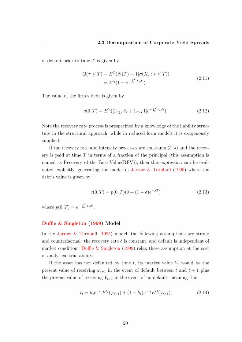
v(0, T ) = EQ([1τ≤T δτ + 1τ>T1]e−∫ T0 rsds). (2.12)
Note the recovery rate process is prespecified by a knowledge of the liability struc-
ture in the structural approach, while in reduced form models it is exogenously
supplied.
If the recovery rate and intensity processes are constants (δ, λ) and the recov-
ery is paid at time T in terms of a fraction of the principal (this assumption is
named as Recovery of the Face Value(RFV)), then this expression can be eval-
uated explicitly, generating the model in Jarrow & Turnbull (1995) where the
debt’s value is given by
v(0, T ) = p(0, T )(δ + (1− δ)e−λT ) (2.13)
where p(0, T ) = e−∫ T0 rsds.
Duffie & Singleton (1999) Model
In the Jarrow & Turnbull (1995) model, the following assumptions are strong
and counterfactual: the recovery rate δ is constant, and default is independent of
market condition. Duffie & Singleton (1999) relax these assumption at the cost
of analytical tractability.
If the asset has not defaulted by time t, its market value Vt would be the
present value of receiving ϕt+1 in the event of default between t and t + 1 plus
the present value of receiving Vt+1 in the event of no default, meaning that
Vt = hte−rtEQ(ϕt+1) + (1− ht)e−rtEQ(Vt+1), (2.14)
20
2.3 Decomposition of Corporate Yield Spreads
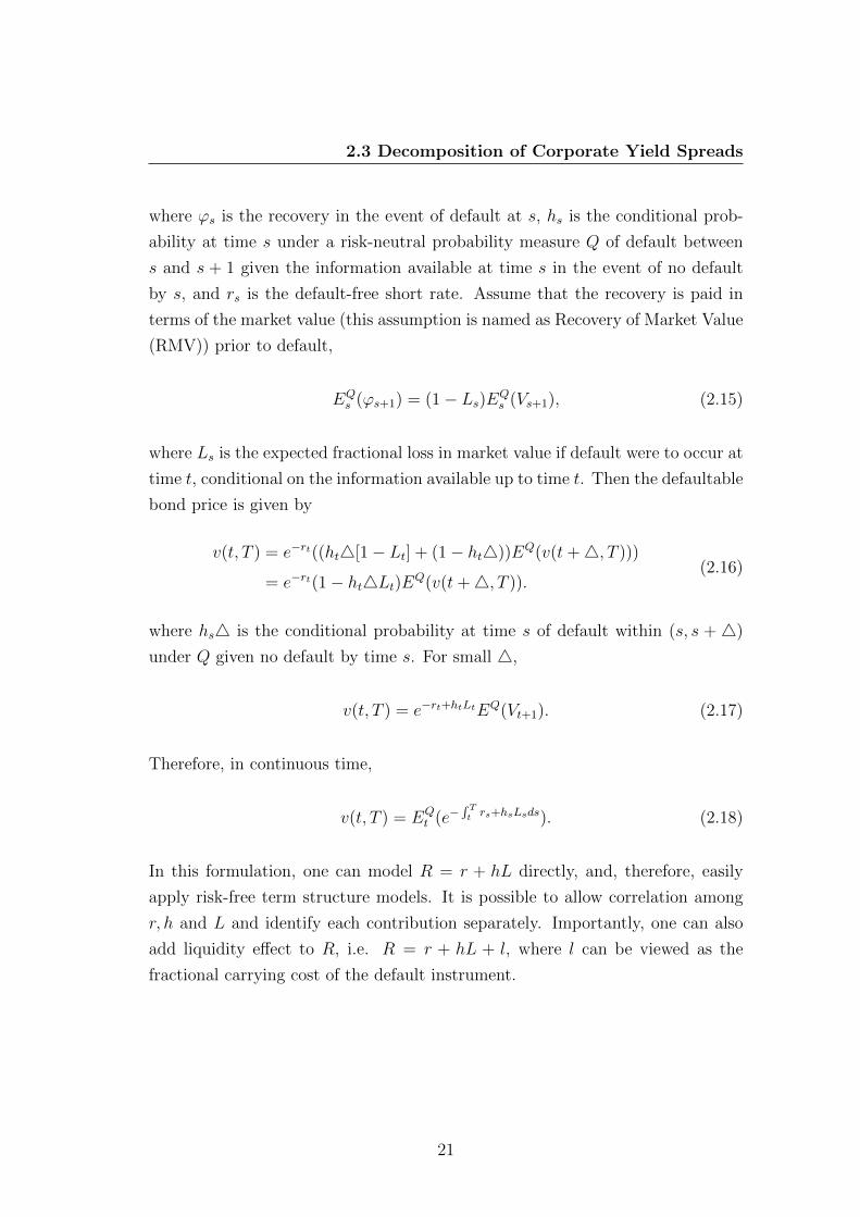
where ϕs is the recovery in the event of default at s, hs is the conditional prob-
ability at time s under a risk-neutral probability measure Q of default between
s and s + 1 given the information available at time s in the event of no default
by s, and rs is the default-free short rate. Assume that the recovery is paid in
terms of the market value (this assumption is named as Recovery of Market Value
(RMV)) prior to default,
EQs (ϕs+1) = (1− Ls)EQ
s (Vs+1), (2.15)
where Ls is the expected fractional loss in market value if default were to occur at
time t, conditional on the information available up to time t. Then the defaultable
bond price is given by
v(t, T ) = e−rt((ht4[1− Lt] + (1− ht4))EQ(v(t+4, T )))
= e−rt(1− ht4Lt)EQ(v(t+4, T )).(2.16)
where hs4 is the conditional probability at time s of default within (s, s +4)
under Q given no default by time s. For small 4,
v(t, T ) = e−rt+htLtEQ(Vt+1). (2.17)
Therefore, in continuous time,
v(t, T ) = EQt (e−
∫ Tt rs+hsLsds). (2.18)
In this formulation, one can model R = r + hL directly, and, therefore, easily
apply risk-free term structure models. It is possible to allow correlation among
r, h and L and identify each contribution separately. Importantly, one can also
add liquidity effect to R, i.e. R = r + hL + l, where l can be viewed as the
fractional carrying cost of the default instrument.
21
2.3 Decomposition of Corporate Yield Spreads
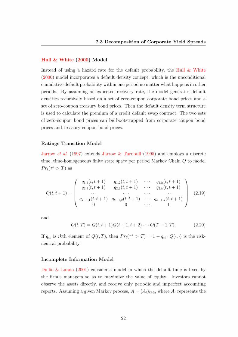
Hull & White (2000) Model
Instead of using a hazard rate for the default probability, the Hull & White
(2000) model incorporates a default density concept, which is the unconditional
cumulative default probability within one period no matter what happens in other
periods. By assuming an expected recovery rate, the model generates default
densities recursively based on a set of zero-coupon corporate bond prices and a
set of zero-coupon treasury bond prices. Then the default density term structure
is used to calculate the premium of a credit default swap contract. The two sets
of zero-coupon bond prices can be bootstrapped from corporate coupon bond
prices and treasury coupon bond prices.
Ratings Transition Model
Jarrow et al. (1997) extends Jarrow & Turnbull (1995) and employs a discrete
time, time-homogeneous finite state space per period Markov Chain Q to model
Prt(τ∗ > T ) as
Q(t, t+ 1) =
q1,1(t, t+ 1) q1,2(t, t+ 1) · · · q1,k(t, t+ 1)q2,1(t, t+ 1) q2,2(t, t+ 1) · · · q2,k(t, t+ 1)· · · · · · · · · · · ·
qk−1,1(t, t+ 1) qk−1,2(t, t+ 1) · · · qk−1,k(t, t+ 1)0 0 · · · 1
(2.19)
and
Q(t, T ) = Q(t, t+ 1)Q(t+ 1, t+ 2) · · ·Q(T − 1, T ). (2.20)
If qik is ikth element of Q(t, T ), then Prt(τ∗ > T ) = 1 − qik; Q(·, ·) is the risk-
neutral probability.
Incomplete Information Model
Duffie & Lando (2001) consider a model in which the default time is fixed by
the firm’s managers so as to maximize the value of equity. Investors cannot
observe the assets directly, and receive only periodic and imperfect accounting
reports. Assuming a given Markov process, A = (At)t≥0, where At represents the
22

2.3 Decomposition of Corporate Yield Spreads
firms value at time t, Duffie & Lando (2001) “obscure” the process A so that it
can be observed at only discrete time intervals, and add independent noise, and
which is observed at times ti for i = 1, ...,∞. The authors derive the distribution
of the firm’s asset value conditional on investors’ information, and, from this
distribution, the intensity of default in terms of the conditional asset distribution
and the default threshold.
Remarks
Many practitioners in the credit trading industry have tended to gravitate to-
ward the reduced form modelling approach given its mathematical tractability.
Jarrow & Protter (2004) argue further that, if one is using the model for risk
management purposes - pricing and hedging - then the reduced form perspective
is the correct one to take. Prices are determined by the market, and the market
reaches equilibrium based on the information that it has available to make its
decisions. In marking-to-market, or judging market risk, reduced form models
are the preferred modelling methodology.
Driessen (2005) provides evidence for a liquidity component in corporate bond
spreads using the Duffie & Singleton (1999) reduced-form pricing approach. They
model the default intensity as a function of several common factors and one firm-
specific factor as well as two terms that allow for correlation with default-free
rates. The liquidity component is modelled by a standard square-root diffusion
process. The model is calibrated using only corporate bonds.
Liu et al. (2006) use a five-factor affine term structure model to jointly model
the Treasury, Repo, and swap term structures and show that the swap spread
is driven by a persistent liquidity process and a rapidly mean-reverting default
intensity process. The state variables follow Gaussian processes with a general
correlation structure.
Another very important and related paper in this strand of the literature is
by Longstaff et al. (2005), who fit a simple reduced-form model to both credit
default swaps and corporate bonds, and find evidence of a significant non-default
component in the yield spread which can be related to the liquidity of a bond.
23

2.3 Decomposition of Corporate Yield Spreads
The ability of reduced form models to price a variety of fixed income and
credit risk products makes them very appealing for our purposes. Moreover, with
the rapid growth of the credit derivatives market, credit default swaps provide a
ideal way to directly measure default risk.
A Credit Default Swap (CDS) is a bilateral financial contract in which one
counterparty (the Protection Buyer) pays a periodic fee, typically expressed in
basis points per annum, paid on the notional amount, in return for a Contingent
Payment by the Protection Seller following a Credit Event with respect to a
Reference Entity. A standard definition of Credit Event1 includes one or more of
the following: bankruptcy, filing for protection, failure to pay, obligation default,
obligation acceleration and repudiation/moratorium.
It is possible, and increasingly easier, to terminate or unwind a credit default
swap before its maturity. In order to exit a credit position in corporate bonds
all the investors have to do is to sell the asset at the market. By contrast, a
CDS position involves negotiating the terms of the unwinding with the original
counterparty (termination), or getting their consent to have a third party step in
the trade in their place (novation or assignment). On a termination, the original
counterparties on the CDS agree to tear up the contact at a MTM price, playable
from Party A to Party B or vice versa depending on which side is in-the-money
at the time. The novation/assignment is more complex in the sense that the
original counterparty (eg. Party B) is required to consent that Party C steps into
the trade to replace Party A. There will be a cash flow between Parties A and C
as in the CDS termination case, and party A will then be out of the picture. The
trade will remain existing, only between Parties B and C from that point on.
There are important differences between corporate bond and CDS worth men-
tioning. A bond investor’s ability to take a certain amount of a specific credit risk
is limited by the possibility of finding such corporate bonds in the marketplace
and the availability of funding for the purchase. Illiquidity can arise from lim-
ited arbitrage in the corporate bond market, as sometimes it can be difficult and
costly to short sell corporate bonds. A CDS investor buying or selling protection,
only needs a fraction of the principal (initial collateral margins or upfront fees),
and the mark-to-market effect of interest rate fluctuations to a position is usually
1Restructuring has been excluded from the CDS contract by ISDA since April 8th, 2009.
24
2.3 Decomposition of Corporate Yield Spreads
negligible. In addition, the availability of CDS is not necessarily linked to the
aggregate amount of reference bonds outstanding, nor their maturities. With the
introduction of the new standard CDS contract and conventions, because of the
generic nature of the cash flows, credit default swaps cannot be demanded partic-
ularly in the way Treasury securities or popular equities may. Furthermore, it is
important to notice that credit default swaps are essentially insurance contracts.
Many investors who buy default protection may intend to hold the position for a
fixed time period.
Therefore, credit default swaps are much less sensitive to market liquidity,
compared to bonds. Ericsson et al. (2005) evaluate the price of default protec-
tion for a sample of US corporations. In bond residuals, they find strong evidence
for non-default components, in particular an illiquidity premium. CDS residuals
reveal no such dependence. This finding supports the assumption in Longstaff
et al. (2005) that CDS spreads do not contain liquidity premium. Blanco et al.
(2005) provide evidence that changes in the credit quality of the underlying name
are likely to be reflected more quickly in the default swap spread than in the
bond yield spread. This may be due to a strongly mean-reverting, non-default
component in bond spreads that obscure the impact of changes in credit qual-
ity. Ericsson et al. (2009) investigate the linear relationship between theoretical
determinants of default risk and default swap spreads. They find that there is
limited evidence for a common factor in residuals, indicating that the liquidity
premium in credit default swap spread is negligible.
As shown in Duffie (1999), under the no-arbitrage condition the credit default
swap premium equals the spread between the par defaultable floating rate note
and the par default-free floating rate note, the credit default swap premium is
a biased measure of the default component in the yield spread of fixed-coupon
corporate bonds. The adjustment from floating-rate spread to fixed-rate spread
can be made explicitly by applying a reduced-form model.
Now, our proposed approach to separate liquidity risk from credit risk is clear.
That is, we extract default intensities by fitting a reduced-form model to CDS
spreads, then use the estimated default intensities to calculate the fair value of
a corporate bond, and finally obtain the non-default price residual by taking the
25
2.3 Decomposition of Corporate Yield Spreads
difference between the fair value and market price. We will discuss in details how
to obtain the non-default price residual or non-default yield spread in Chapter 3.
2.3.3 Decomposition by regressions
A common feature of empirical research in liquidity is that it generally uses
transaction data such as trading volume, number of trades or the bid-ask spread
to construct measures of illiquidity. Empirical papers which examine liquidity in
bond or equity markets use both direct measures (based on transaction data), and
indirect measures (based on bond characteristics and/or last prices). However,
transaction data for illiquid securities are often rather sparse. Researchers have
to resort to indirect proxies. The most popular approach is to regress the yield
spreads on a range of proxies for credit risk, liquidity risk and other effects.
Meanwhile, panel regression analysis is often applied to take advantage of huge
data sets which contains cross-sectional time series data (e.g. time series of prices
of different bonds), as some measures are homogenous across individual bonds
but vary over time and others are invariant through time but different cross-
sectionally.
Measures of Illiquidity
We will now review some illiquidity measures frequently used in the empirical
liquidity literature. Our focus will be mainly on the recent literature.
Direct illiquidity measures include price impact, transaction cost, trading fre-
quencies and trading volume. Microstructure theory suggests that the transaction
cost combined with the price impact of trade is a good measure of an asset’s liq-
uidity.
Amihud (2002) examines the effect of illiquidity on the cross-section of stock
returns using an illiquidity measure that is related to Kyle (1985) price impact
coefficient λ. The measure is called ILLIQ = |R|/(P ∗ V OL), where R is daily
return, P is the closing daily price and V OL is the number of shares traded
during the day. ILLIQ reflects the relative price change that is induced by a
given dollar volume. The Amihud illiquidity measure has been used extensively
26
2.3 Decomposition of Corporate Yield Spreads
in the literature on equity. When applied to bond markets, this measure can be
defined as
ILLIQ =|pt − pt−1|/pt−1
Qt
(2.21)
where pt is the bond price and Qt is the dollar volume of a trade. Larger values
of the Amihud measure suggest more illiquid bonds, as a given trade size moves
prices more.
Transaction costs cause negative serial dependence in successive observed mar-
ket price changes. The bond price bounces back and forth within the bid-ask
bounce, and higher bid-ask bounces lead to higher negative covariance between
adjacent price changes. Assuming market efficiency, the effective bid-ask spread
can be measured by St = 2√−cov(4Pi,4Pi−1) where“cov” is the first-order
serial covariance of price changes, t is the time period for which the measure is
calculated and 4 represents the adjacent price difference. This is the famous
Roll measure Roll (1984). Two assumptions are needed: The asset is traded in
an informationally efficient market, and the probability distribution of observed
price changes is stationary. Roll’s model generates undefined spread estimates
almost half of the time when applied to daily transaction data on equities [Harris
(1990)]. It may also suffer from misspecification problem when applied to markets
with richer structures. However, despite of its simplicity, it is still very useful as
it provides a method to estimate the bid-ask spread based on only transaction
prices. Later in section ?? we will discuss Roll’s model and its extensions in
detail.
Mahanti et al. (2009) investigate the interaction between market liquidity
and the price of credit risk by relating the liquidity of corporate bonds to the
basis between the credit default swap price of the issuer and the par-equivalent
CDS spread of the bond. The liquidity of a bond is measured by the so-called
latent liquidity which is defined in Mahanti et al. (2007) as the weighted average
turnover of the investors holding the bond, where the weights are their fractional
holdings of the bond. They find that their measure has explanatory power for
the liquidity component of the CDS-bond basis.
Chen et al. (2007) investigate bond-specific liquidity effects on the yield spread
using three separate liquidity measures, namely bid-ask spread, the liquidity
27

2.3 Decomposition of Corporate Yield Spreads
proxy of zero returns and a model-based transaction cost estimator developed
by Lesmond et al. (1999). In the presence of transaction costs, investors will
trade less frequently. Bekaert et al. (2007) suggest that the magnitude of the
percentage of zero returns is a reasonable measure of illiquidity. Lesmond et al.
(1999) show that their estimator measures the underlying liquidity costs better
than the percentage of zero returns. They find that liquidity is priced in both
the levels and the changes of the yield spread. In our study we are also interested
in the cross-sectional differentials of both the level of liquidity and the liquidity
premium across individual bonds. However, unlike their study, we will be able
to make use of the information from the credit default swap market to control
credit risk, and examine the interaction between credit and liquidity risk.
Bao et al. (2011) examine the connection between their Roll measure and
bond trading activity measures (e.g. trade size, number of trades and turnover).
They find that bonds which have smaller trade sizes are more illiquid. Bond
trading activity measures may be able to capture the liquidity variations at the
individual bond level.
Indirect illiquidity measures include bond characteristics such as issue size or
outstanding amount, time-to-issue or time-to-maturity, and price volatility.
The earliest example of this kind of research on corporate bonds, that we
know of, is by Fisher (1959), who uses the amount outstanding of a bond as a
measure of liquidity and the earnings variability as a measure of the credit risk of
the firm, and finds that yield spreads on bonds with low issue sizes are higher. As
we discussed earlier, one of the sources of illiquidity is related to searching costs.
This searching friction is particularly relevant in over-the-counter markets such
as the corporate bond market. The amount outstanding measures the overall
availability of a bond, and therefore, reflects the liquidity of a bond.
Time-Since-Issue and Time-To-Maturity are popular proxies for bond liquid-
ity. Examining the corporate bond market, Schultz (2001) finds that newly issued
bonds trade more than old bonds. More recently, Edwards & Piwowar (2007)
study secondary transaction costs in the corporate bond markets. They find that
transaction costs decrease significantly with trade size, and highly rated bonds,
recently issued bonds, and bonds close to maturity have lower transaction costs
than do other bonds.
28

2.3 Decomposition of Corporate Yield Spreads
Alexander et al. (2000) find that bond issues with higher volume tend to be
larger and more recently issued. Bao et al. (2011) establish a robust connec-
tion between their illiquidity measure and liquidity-related bond characteristics.
Similarly, they find that the illiquidity measure is higher for older and smaller
bonds, and bonds with smaller average trade sizes and higher idiosyncratic return
volatility. These papers not only find strong evidence of a seasoning effect, but
also they both suggest that issue amount could be an indicator of bond liquid-
ity. Intuitively, bonds with smaller issue amount tend to be held by long-term
investors more easily, reducing the tradable amount and thus their liquidity.
Moreover, in the microstructure literature, market makers’ inventory holding
costs are often related to price volatility. Alexander et al. (2000) use the average
of absolute price returns to approximate the underlying volatility. However, they
find a negative relation between volatility and yields. Gwilym et al. (2002) con-
duct an examination of the determinants of the bid-ask spread and confirm that
credit rating, issue size, and price volatility affect liquidity.
Houweling & Vorst (2005) use liquidity-sorted portfolios in the European mar-
ket to test whether liquidity risk is priced by using nine proxies for liquidity in-
cluding issued amount, listing, currency, on-the-run or not, age, whether there
are missing prices, yield volatility, the number of quote contributors, and yield
dispersion.
Dick-Nielsen et al. (2012) analyze liquidity components of corporate bond
spreads by using TRACE data. They find that illiquidity premia increased dra-
matically during the crisis. As no liquidity measure is perfect and any measure
is able to capture some information about liquidity, they combine four liquid-
ity proxies, namely the price impact of trades(the Amihud measure), transaction
costs(Unique roundtrip cost) and the variability of these two variables, to capture
most of the liquidity-related variation of spreads.
In addition to the above research on the corporate bond market, by Covitz &
Downing (2007) find that liquidity plays a role in the determination of spreads
of commercial papers (CP), but credit quality is a more important determinant
of spreads. Their regression analysis is based on three liquidity measures (that
is trade volume, dollar volume and maturity) and three credit risk proxies (that
is Expected Default Frequency (EDF), credit rating and equity volatility). Li
29

2.3 Decomposition of Corporate Yield Spreads
et al. (2009) estimate a market-wide liquidity factor based on transaction data
and document a strong positive relation between expected Treasury returns and
liquidity. Their findings suggest that term structure modelling should consider
liquidity effects in order to capture yield curve dynamics.
Some researchers are interested in cross-market determinants of liquidity.
Chordia et al. (2005) explores cross-market liquidity dynamics by estimating a
vector autoregressive model for liquidity. They find that shocks to stock and
bond market liquidity and volatility are significantly correlated, implying that
common factors drive liquidity and volatility in these markets. Using time-series
regressions, controlling for market risk by using the stock market index return
and the change in implied equity index volatility, De Jong & Driessen (2007)
provide evidence that corporate bond returns are positively related to changes in
the equity and bond market liquidity measures.
The recent liquidity crisis in the interbank lending market warns us that great
attention has to be paid to the healthy functioning of this market, which is directly
related to the monetary policy of governments. Eisenschmidt & Tapking (2009)
propose a theoretical model for the funding liquidity risk of lenders in unsecured
term money markets and presents evidence that the unsecured interbank money
market rates reached levels that cannot be explained alone by higher credit risk.
Michaud & Upper (2008) and Taylor and Williams (2008)Taylor & Williams
(2009) try to decompose money market rates into credit risk, liquidity and other
components by applying regression techniques. Treated as independent variables,
the credit component is measured by CDS spreads and liquidity is measured by
dummy variables or treated as a residual. They demonstrate a significant impact
of liquidity on money market rates.
Remarks
As we can see, each liquidity measure has its strengths and weaknesses. More-
over, some measures are able to explain cross-sectional differences whereas other
measures capture common time series variations. We will use both direct and in-
direct measures in our panel regression analysis, as one of problems is how much
of the variations in the level of liquidity and liquidity premium are common and
30
2.3 Decomposition of Corporate Yield Spreads
how much are idiosyncratic. Panel regression techniques will be reviewed in the
next section.
2.3.4 Panel Data Analysis
Our data consist of a battery of corporate bonds and credit default spreads. These
data enable us to observe not only time series but also cross-sectional variations
in the level of liquidity as well as the liquidity premium. Recent developments in
econometric technique and statistical software offer us some great tools to analyze
panel data. In this section we will review some important issues in panel data
analysis. In particular, we will discuss two special cases, namely fixed-effects and
random-effects models1, followed by diagnostic tests.
Fixed-Effects and Random-Effects
Consider fitting models of the form
yit = α + xitβ + νi + εit. (2.22)
In this model, νi + εit is the residual, which we have little interest in; we
want estimates of β or perhaps α. νi is the unit-specific residual; it differs be-
tween units, but for any particular unit, its value is constant. εit is the “usual”
residual with the usual properties (mean 0, uncorrelated with itself, uncorrelated
with independent variables, uncorrelated with unit-specific residual νi, and ho-
moscedastic).
If equation 2.22 holds, we must have that
yi = α + xiβ + νi + εi, (2.23)
where yi =∑
t yit/Ti, xi =∑
t xit/Ti, and εi =∑
t εit/Ti. Subtracting equation
1Both Baltagi (2008) and Wooldridge (2009) provide good overviews of fixed-effects andrandom-effects models. Allison (2009) provides perspective on using fixed-effects and random-effects models.
31
2.3 Decomposition of Corporate Yield Spreads
2.23 from equation 2.22, we obtain
(yit − yi) = (xit − xi)β + (εit − εi). (2.24)
Equation 2.24 provides the fixed-effects (FE) estimator.
Fixed-effects (FE) should be applied if one is only interested in analyzing
the impact of variables that vary over time. FE explore the relationship between
predictor and outcome variables within an entity (country, person, company, etc.).
Each entity has its own individual characteristics which may or may not influence
the predictor variables. When using FE it is assumed that something within the
entity may impact or bias the predictor or outcome variables and we need to
control for this. This is the rationale behind the assumption of the correlation
between the entity’s error term and predictor variables. FE remove the effect of
those time-invariant characteristics from the predictor variables so we can assess
the predictors’ net effect.
Another important assumption of the FE model is that those time-invariant
characteristics are unique to the individual and should not be correlated with
other individual characteristics. Each entity is different, therefore, the entity’s
error term and the constant (which captures individual characteristics) should
not be correlated with other entities’ error terms and the constants. If the error
terms are correlated, then FE is not suitable any more, since inferences may
not be correct and you need to model that relationship (probably using random-
effects). In other words, the FE model controls for all time-invariant differences
between the individuals, so the estimated coefficients of the FE models cannot
be biased because of omitted time-invariant characteristics.
One side effect of the features of FE models is that they cannot be used to
investigate time-invariant causes of the dependent variables. Technically, time-
invariant characteristics of the individuals are perfectly collinear with the entity
dummies. FE models are designed to study the causes of changes within an
entity. A time-invariant characteristics cannot cause such a change, because it
is constant for each entity. In this case, one may resort to the random-effects
models.
32
2.3 Decomposition of Corporate Yield Spreads
The random-effects (RE) estimator turns out to be equivalent to estimation
of
(yit − θyi) = (1− θ)α + (xit − θxi)β + (1− θ)νi + (εit − θεi), (2.25)
where θ is a function of σ2ν and σ2
ε . If σ2ν = 0, meaning that νi is always 0, then
θ = 0 and equation 2.22 can be estimated by OLS directly. Otherwise, if σ2ε = 0,
meaning that εit is 0, then θ = 1 and the FE estimator returns all the information
available.
The rationale behind random effects (RE) model is that, unlike the FE model,
the variation across entities is assumed to be random and uncorrelated with the
predictor and with independent variables included in the model. An advantage of
RE is that it is possible to include time invariant variables. In the FE model these
variables are absorbed by the intercept. RE assume that the entity’s error term
is not correlated with the predictors which allows for time-invariant variables to
play a role as explanatory variables. In RE one needs to specify those individual
characteristics which may or may not influence the predictor variables. The
problem with this model is that some variables may not be available, therefore,
leading to omitted variable bias in the model.
Diagnostic Tests
According to Baltagi (2008), cross-sectional dependence is a problem in macro
panels with long time series. This is not much of a problem in micro panels. The
null hypothesis in the Breusch-Pagan LM test of independence is that residuals
across entities are not correlated. Alternatively, Pasaran’s CD test can be used
to test whether or not the residuals are correlated entities. The null hypothesis is
that residuals are not correlated. If cross-sectional dependence is present, it can
be corrected by using Driscoll and Kraaay standard errors (See Driscoll & Kraay
(1998)).
A modified Wald test and a likelihood ratio test for groupwise heteroscedas-
ticity are developed (See Baum (2006)). The null hypothesis is homoscedasticity
or constant variance . If the tests show that there is heteroscedasticity, then it
33
2.3 Decomposition of Corporate Yield Spreads
can be corrected by using robust standard errors or Huber-White standard errors
(See Green (2008) and White (1980)).
The disturbances may be serially correlated within the panel. Serial correla-
tion causes the standard errors of the coefficients to be smaller than they actually
are and higher R-squared values. A Lagram-Multiplier test for serial correlation
is derived by Wooldridge (2002). The null hypothesis is no serial correlation.
When first-order autocorrelation is present, then it can be corrected by using
Prais-Winsten estimation (See Wooldridge (2009)).
Additionally, to decide between fixed or random-effects one can run a Haus-
man test where the null hypothesis is that the preferred model is random-effects
against fixed-effects (See Green (2008)).
34
2.4 Estimation of the Effective Bid-ask Spread
2.4 Estimation of the Effective Bid-ask Spread
In the market microstructure literature on estimating and decomposing the bid-
ask spread, there are two classes of models: the serial covariance spread estimation
model, and the order flow spread estimation model. We found existing models
suffered from misspecification problems when applied to our data. Therefore, we
also review some techniques which may help when we develop our models.
2.4.1 Serial Covariance Spread Estimation Model
In the serial covariance spread estimation model, the spread measures are derived
from the serial covariance properties of transaction price changes.
Roll (1984) Model
The first such model was developed by Roll (1984). Transaction costs are inferred
from serial covariance of daily equity returns. In an efficient market the price
dynamics may be stated as
mt = mt−1 + εt, (2.26)
pt = mt + sqt, (2.27)
where mt is the unobservable efficient price, pt is the transaction price observed
at time t, s is one-half the bid-ask spread, and the qt are trade direction indi-
cators, which take the values +1 for buy orders or −1 for sell orders with equal
probability.
The changes in transaction prices between two successive trades is
pt − pt−1 = mt + sqt − (mt−1 + sqt−1), (2.28)
∆pt = s∆qt + εt. (2.29)
35

2.4 Estimation of the Effective Bid-ask Spread
Thus,
Cov(∆pt,∆pt−1) = E[∆qt∆qt−1s2] + E[∆qtεt−1s]
+ E[∆qt−1εts] + E[εtεt−1],(2.30)
where Cov(∆pt,∆pt−1) is the first-order autocovariance of the price changes.
In deriving the Method of Moments estimator Roll (1984) makes several as-
sumptions:
1. Successive transaction types are independent. Thus,
E[qtqt−1] = 0.
2. The half-spread s is constant.
3. Order flows do not contain information about future fundamental price
changes. Thus,
E[∆qt−1εt] = 0.
4. Changes in fundamental value cannot predict order flows:
E[∆qtεt−1] = 0.
5. The innovations in the fundamental price process reflect public information
and are assumed to be independent. Therefore,
E[εtεt−1] = 0.
Then,
Cov(∆pt,∆pt−1) = −s2. (2.31)
This gives Roll’s Method of Moments spread estimator
s =√−Cov(∆pt,∆pt−1). (2.32)
36

2.4 Estimation of the Effective Bid-ask Spread
If the innovations in the efficient price process are assumed to follow a normal
distribution with mean 0 and constant variance σ2ε , the Method of Moments
variance estimator is
σ2ε = V ar(∆pt)− s2V ar(∆qt) = V ar(∆pt)− 2s2. (2.33)
An advantage of Roll’s model is that it relies exclusively on transaction price
data.
Choi et al. (1988)) Model
Choi et al. (1988) modify Roll’s estimator and introduce a serial correlation as-
sumption regarding transaction type. An implicit hypothesis in Roll’s model is
that orders are not serially correlated, meaning that the probability of a buy order
is equal to that of a sell order, and is independent of the previous orders. However,
when large orders are broken up, there could be serial dependence transaction
type.
The probability of continuation is equal to
Pr(∆qt+1 = ∆qt) = (1− γ), (2.34)
and the covariance between the transaction price variations results in
Cov(∆pt,∆pt−1) = −s2γ2. (2.35)
whereas the spread estimator becomes
s =1
γ
√−Cov(∆pt,∆pt−1). (2.36)
Stoll (1989) Model
The probability of an order flow reversal or continuation may be different from12
when market makers adjust bid-ask spreads to equilibrate inventory. Stoll
37
2.4 Estimation of the Effective Bid-ask Spread
(1989) models the relation between the bid-ask spread and the serial covariance
of transaction price changes as a function of the probability of a price reversal
and the magnitude of a price reversal in order to decompose the bid-ask spread
into three components: adverse information costs, order processing costs, and
inventory holding costs. The model consists of two equations:
Cov(∆pt,∆pt−1) = s2[δ2(1− 2π)− π2(1− 2δ)], (2.37)
Cov(∆Mt,∆Mt−1) = δ2s2(1− 2π), (2.38)
where Mt is mid-quote which is calculated as the midpoint of the bid-ask quotes
that prevail just before a transaction, δ = ∆pt|pt−1=At−1,pt=Ats
= −∆pt|pt−1=Bt−1,pt=Bts
is the magnitude of a price continuation as a percentage of the bid-ask spread.
He shows that the compensation earned by a market maker for order processing
and inventory costs is 2(π − δ)s. The remainder of the spread [1 − 2(π − δ)]s
reflects the adverse selection costs.
George et al. (1991) Model
George et al. (1991) use daily data and consider changing expectations in their
model. As in Roll’s model, they also assume thet the spread is independent of
trade size and the probabilities of trades at the bid and ask are equal. Their
model for transaction prices can be written as
pt = mt + πsqt, (2.39)
mt = Et +mt−1 + (1− π)sqt + νt, (2.40)
where the “true” expected return of a security, Et, is varying over time.
38
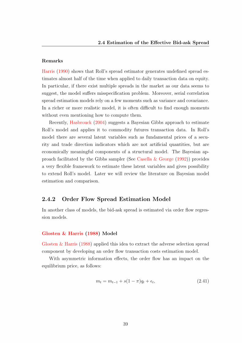
2.4 Estimation of the Effective Bid-ask Spread
Remarks
Harris (1990) shows that Roll’s spread estimator generates undefined spread es-
timates almost half of the time when applied to daily transaction data on equity.
In particular, if there exist multiple spreads in the market as our data seems to
suggest, the model suffers misspecification problem. Moreover, serial correlation
spread estimation models rely on a few moments such as variance and covariance.
In a richer or more realistic model, it is often difficult to find enough moments
without even mentioning how to compute them.
Recently, Hasbrouck (2004) suggests a Bayesian Gibbs approach to estimate
Roll’s model and applies it to commodity futures transaction data. In Roll’s
model there are several latent variables such as fundamental prices of a secu-
rity and trade direction indicators which are not artificial quantities, but are
economically meaningful components of a structural model. The Bayesian ap-
proach facilitated by the Gibbs sampler (See Casella & George (1992)) provides
a very flexible framework to estimate these latent variables and gives possibility
to extend Roll’s model. Later we will review the literature on Bayesian model
estimation and comparison.
2.4.2 Order Flow Spread Estimation Model
In another class of models, the bid-ask spread is estimated via order flow regres-
sion models.
Glosten & Harris (1988) Model
Glosten & Harris (1988) applied this idea to extract the adverse selection spread
component by developing an order flow transaction costs estimation model.
With asymmetric information effects, the order flow has an impact on the
equilibrium price, as follows:
mt = mt−1 + s(1− π)qt + εt, (2.41)
39

2.4 Estimation of the Effective Bid-ask Spread
where π is the parameter indicating order processing costs as a fraction of total
costs, and (1 − π) the fraction of adverse selection costs. This implies that the
equilibrium price includes the public information as well as the private informa-
tion revealed by the order flow qt.
If the ‘true’ price reflects adverse selection costs, then the transaction price pt
reflects order processing costs:
pt = mt + sqt. (2.42)
They allow the order processing cost and adverse selection cost to be function
of trade size. Assume the spread consists of an order processing cost component,
ct, and a price impact component, zt:
st = ct + zt. (2.43)
Both spread components are linear in trade size vt:
ct = c0 + c1vt, (2.44)
zt = z0 + z1vt. (2.45)
The model is estimated by Maximum Likelihood and intraday data on prices
and trading volume (or net order flow) are needed.
Madhavan et al. (1997) Model
Madhavan et al. (1997) develop an order flow regression model based on Glosten
& Harris (1988) to study intra-day patterns in bid-ask spreads, price volatility,
the serial correlations of transaction returns and quote revisions. Their model
can be written as
∆pt = (φ+ θ)qt − (φ+ ρθ)qt−1 + et (2.46)
40

2.4 Estimation of the Effective Bid-ask Spread
where θ is the adverse selection component, φ is the order processing and inven-
tory component. θ measures the degree of information asymmetry. Higher values
of θ indicate larger revisions for a given innovation in order flow. φ represents
market makers’ cost per share for supplying liquidity. Thus, φ captures the tran-
sitory effect of order flow on prices. ρ is the first-order autocorrelation of order
flow. When order flow is serially uncorrelated, ρ is equal to 0. Their model also
assumes a fixed order size.
Huang & Stoll (1997) Model
Huang & Stoll (1997) develop a model to decompose the components of the bid-
ask spread. In particular, the spread components differ according to trade size.
Let us look at their model in details.
The unobservable fundamental value mt follows:
mt = mt−1 + αsqt−1 + εt, (2.47)
where α is the percentage of the half-spread contributable to asymmetric informa-
tion. Assuming that past trades are of a normal size of one, the quote midpoint
is related to the fundamental value according to
Mt = mt + βst−1∑i=1
qi, (2.48)
where β is the proportion of the half-spread attributable to inventory holding
costs, and∑t−1
i=1 qi is the cumulated inventory from the market open until time
t− 1 with q1 as the initial inventory for the day. The transaction price follows
pt = Mt + sqt + ηt, (2.49)
where ηt captures the deviation of the observed half-spread from the constant
half-spread as well as rounding errors associated with price discreteness.
41

2.4 Estimation of the Effective Bid-ask Spread
Combining the above equations, the model can be written as the form of
observed price changes:
∆pt = s(qt − qt−1) + λsqt−1 + et, (2.50)
where λ = α+ β and et = εt + ∆ηt. The model provides estimates of the traded
spread, s, and the total adjustment of quotes to trades, λs.
In particular, they also generalize the model to allow coefficient estimates
depending on three trader size categories. Then, the model becomes
∆pt = ssqst+(λs−1)ssqst−1+smqmt +(λm−1)smqmt−1+slqlt+(λl−1)slqlt−1+et, (2.51)
where the half-spread s and λ differ for small, medium, and large trade sizes.
Ball & Chordia (2001) Model
Ball & Chordia (2001) generalize the Huang & Stoll (1997) model by explicitly
allowing for rounding onto the tick grid. More importantly, they allow the bid-
ask spread to vary from transaction to transaction and to continuously depend
on prior trade size and market depth. Similar to our approach in the first study,
the chosen model is determined by the marginal likelihood computed from the
Gibbs sampling output as suggested by Chib (1995).
The transaction price is modeled as follows:
pt = [mt + (1− λ)stqt]Round, (2.52)
where λ is the adverse selection component of the spread and the notation [.]Round
represents rounding onto the tick grid. The unobservable fundamental value is
assumed to evolve as follows:
mt = mt−1 + λstqt + ut. (2.53)
Here they allow the adverse selection to affect the fundamental value.
42

2.4 Estimation of the Effective Bid-ask Spread
They argue that the bid-ask spread may vary according to a micro information
flows and responding to large information-related trades. Therefore, they model
the bid-ask spread as follows:
ln(st) = α + βln(st−1) + δln(Vt−1/Dt−1) + τTIMEt−1 + d1BEG+ d2END + et.
(2.54)
where Vt−1 is the volume at the previous trade, Dt−1 is the corresponding depth
of trade for which the then prevailing bid-ask quote held, TIMEt−1 is the time
between the last trade and the one before it, and BEG(END) are dummy vari-
ables to represent the first (last) hour of the trading day. The model allows the
spread to depend on the volume and depth of previous transaction. The dummy
variables capture the intra-day seasonality.
They have observations on the transaction price, the trade direction, the size
and depth of the previous trade, and the time between trades as well as whether
the trade occurred at the beginning or end of the trading day. However, the latent
variables the fundamental value and the effective bid-ask spread are unknown.
The model is estimated by using Bayesian estimation method which provides a
relaxable framework to estimate the model parameters and the latent variables
given the observed data. The development in Bayesian econometric provides
an opportunity and reflexibility to estimate such complicated models as Ball
& Chordia (2001) model and our model in Chapter 3. With such a powerful
technique in hand, we will be able to develop a model whose structure is rich
enough to fit the market observations better.
Within a Bayesian framework we can also choose the best model from various
alternative specifications. For instance, Ball & Chordia (2001) consider four
alternative model specifications:
• M1: d1 = d2 = τ = 0,
• M2: d1 = d2 = 0,
• M3: τ = 0,
• M4: No restriction on the parameters.
43

2.4 Estimation of the Effective Bid-ask Spread
The first model assumes the spread is a first order autoregressive process and also
depends on the transaction size V and the depth D. The intuition is that the
greater the prior volume per unit depth, the wider the spread will become. The
second and third models capture the time-between-trades and intro-day effects
on the spread. The best model is chosen by comparing the marginal likelihood
computed using the Gibbs outputs from the estimation stage. Standard Markov
Chain Monte Carlo methods such as Gibbs sampling and Metropolis-Hastings
sampling will be reviewed later on.
Remarks
As explained by Hasbrouck (2004), in the serial correlation spread estimation
models, important latent variables such as bids, asks, efficient prices and trade
directions, which are economically meaningful information, are ignored. Modern
Bayesian econometric techniques boost the development of the order flow spread
estimation model. Equipping Bayesian econometrics, order flow spread estima-
tion models are able to capture a variety of market structures, e.g. the underlying
value process may depend on volume or depth, the bid-ask spread may take mul-
tiple values or vary continuously over time. Under Bayesian framework, one may
also infer the trade directions from the transaction data, although there exist
some simple rules to help us classify trades. However, Bayesian approach often
does not have close-form solution, and is not very attractive analytically. With
large data set or more parameters, the numerical estimation procedure may take
several hours or more to finally converge. Nevertheless, given many advantages
that the Bayesian approach has given, our extended models follow this approach.
In the following we will first review the literature on trade classification and
discuss their advantages and problems before introducing some Bayesian econo-
metric techniques recently developed, including Markov Chain Monte Carlo meth-
ods, Bayesian model selection, State space model and Kalman filer.
44

2.4 Estimation of the Effective Bid-ask Spread
2.4.3 Trade Classification
The data series of some products do not contain information about buy/sell
identifier for trades. However, trade classification is useful in the estimation of
the net order flow, the probability of informed trading, and the effective bid-ask
spread.
When bid-ask quotes are available, a natural method is to compare the trade
price with the quotes prevailing at the time of the trade. A trade is classified
as a buy trade if the transaction price is above the midpoint of the bid-ask
quotes. Trades below the midpoint will be classified as sells. The limitation of
this algorithm is that transactions executed at the midpoint cannot be classified
by the quote rule.
When bid-ask quotes are not available, a technique known as a ‘tick test’
is commonly used. Each trade is classified by the test into four categories: an
uptick, a downtick, a zero uptick, and finally a zero downtick. A trade will be
classified as an uptick (downtick) if the price is higher (lower) than the price prior
to the trade. When the price is the same as the previous price, if the last price
change was an uptick (downtick), then the trade is a zero-uptick (zero downtick).
A trade will be classified as a buy if it is an uptick or a zero uptick; otherwise it
will be classified as a sell. Similarly, a reverse ‘tick test’ uses the next trade price
to classify the current trade. If the next trade occurs on an uptick or zero uptick
(a downtick or zero downtick), the current trade will be classified as a sell (buy).
The third rule is a hybrid method, suggested by Lee & Ready (1991). Lee &
Ready (1991) method combines the quote rule and the tick rule by first classify all
trades that do not occur at the midpoint using the quote rule, and then classify
midpoint trades by the ‘tick test’. Using intra-day quote and trade prices on
equity, Finucane (2000) finds that using either Lee & Ready (1991) algorithm or
the ‘tick test’ results in significantly biased estimates of effective bid-ask spreads
and signed volume, however, the ‘tick test’ performs better than Lee & Ready
(1991) algorithm.
Using a Nasdaq proprietary data set, Ellis et al. (2000) find that the quote
rule, the tick rule, and the Lee & Ready (1991) rule correctly classify 76.4%,
77.66%, and 81.06% of the trades, respectively. But all rules do not enjoy much
45

2.4 Estimation of the Effective Bid-ask Spread
success in classifying trades executed inside the quotes. Therefore, Ellis et al.
(2000) propose a new classification rule: all trades executed at the ask (bid)
quote are classified as buys (sells). All other trades are classified by the ‘tick
test’. They show the new algorithm outperforms other classification rules.
2.4.4 Markov Chain Monte Carlo Method
Markov chain Monte Carlo (MCMC) methods are a class of algorithms for sam-
pling from probability distributions based on constructing a Markov chain that
has the desired distribution as its equilibrium distribution. The state of the chain
after a large number of steps is then used as a sample of the desired distribution.
The quality of the sample improves as a function of the number of steps. The
first such method is known as the Metropolis-Hastings (MH) algorithm (See Chib
& Greenberg (1995)). Another MCMC method is the Gibbs Sampling algorithm
(See Casella & George (1992)). Now we will briefly review these two algorithms.
Metropolis-Hastings
The general idea of the Metropolis-Hastings algorithm (Hastings (1970)) is to
generate a series of samples that are linked in a Markov chain. The MH algorithm
is an extension of the original Metropolis algorithm (Metropolis et al. (1953)).
The candidate-generating density is denoted q(x, y), where∫q(x, y)dy = 1.
This density can be interpreted as that when a process is at the point x, the den-
sity generates a value of y from q(x, y). If q(x, y) does not satisfy the reversibility
condition, for some x, y,
π(x)q(x, y) > π(y)q(y, x), (2.55)
where π(.) is the density from which we would like like to generate sample but
the transition kernel is unknown. A possible way is to introduce a probability
α(x, y) < 1 such that the reversibility condition is satisfied. Then,
π(x)q(x, y)α(x, y) = π(y)q(y, x). (2.56)
46
2.4 Estimation of the Effective Bid-ask Spread
Thus,
α(x, y) = π(y)q(y, x)/π(x)q(x, y). (2.57)
Therefore the transitions from x to y (y 6= x) are made according to pMH(x, y) =
q(x, y)α(x, y). In order for pMH(x, y) to be reversible, the probability of move
must be set to
α(x, y) = min[π(y)q(y, x)/π(x)q(x, y), 1], (2.58)
α(x, y) = min[π(y)q(y, x)/π(x)q(x, y), 1], if π(x)q(x, y) > 0, (2.59)
= 1, otherwise. (2.60)
In summary, the MH algorithm starts with an arbitrary value x(0):
1. Repeat for j = 1, 2, ..., N .
2. Generate y from q(x(j), ·) and u from u(0, 1).
3. If u ≤ α(x(j), , y), set x(j+1) = y.
4. Else set x(j+1) = x(j).
5. Return x(1), x(2), ..., x(N).
Gibbs Sampling
The Gibbs sampling is a technique for generating random variables from a marginal
distribution indirectly, without having to calculate the joint density. As a Markov
chain Monte Carlo method (Chib & Greenberg (1996)), the Gibbs sampler gen-
erates sample values from the distribution of each variable in turn, conditioned
on the current values of the other variables.
Suppose we are given a joint density f(x, y1, ..., yp), and are interested in
obtaining characteristics of the marginal density
f(x) =
∫...
∫f(x, y1, ..., yp)dy1...dyp, (2.61)
47
2.4 Estimation of the Effective Bid-ask Spread
such as the mean or variance. The most natural and straightforward way would
be to calculate f(x) and use it to obtain the desired characteristic. However, there
are many situations where such a integration in equation (2.61) are not available
in closed form or difficult to compute numerically. In such cases the Gibbs sampler
provides an alternative method for obtaining the marginal density.
Instead of computing f(x) directly, the Gibbs sampler allows us effectively to
generate a sample X1, ..., Xm ∼ f(x) without requiring f(x). By simulating a
large enough sample, the mean, variance, or any other characteristic of f(x) can
be calculated to the desired degree of accuracy.
Let us consider a bivariate random variable (x, y), and suppose we would like
to compute marginal densities, p(x) and p(y). The idea of Gibbs sampler is that
it would be easier to consider in terms of a sequence of conditional distributions,
p(x|y) and p(y|x), than it is to consider in terms of the marginal densities by
integrating the joint density p(x, y) over x or y.
The sampler starts with some initial values x(0) for x . Then we can obtain y(0)
by generating a random variable from the conditional distribution p(y|x = x(0)).
The sample uses y(0) to generate a new value x(1), drawing from the conditional
distribution p(x|y = y(0)). The Gibbs sampler continues as follows:
y(i) ∼ p(y|x = x(i−1)), (2.62)
x(i) ∼ p(x|y = y(i)). (2.63)
This process is repeated for k times, generating a sequence of length k, where a
subset of pairs (x(j), y(j)) for 1 ≤ m ≤ j < k are taken as the draws from the
full joint distribution. The Gibbs sequence converges to a stationary distribution
which is the target distribution.
2.4.5 Bayesian Model Comparison
Bayes factors have been considered as alternatives to classical P -values for testing
hypotheses and for quantifying the degree to which observable data support or
48

2.4 Estimation of the Effective Bid-ask Spread
conflict with a hypotheses. Bayesian model comparison can be based on Bayes
factors (Kass & Raftery (1995)). An alternative option is the Deviance Informa-
tion Criterion (DIC) developed by Spiegelhalter et al. (2002).
Bayes Factors
We begin with data D, assumed to be have arisen under one of the two hypothe-
ses H1 and H2 according to a probability density Pr(D|H1) or Pr(D|H2). Given
a prior probabilities Pr(H1) and Pr(H2) = 1− Pr(H1), the data produce a pos-
terior probabilities Pr(H1|D) and Pr(H2|D) = 1−Pr(H1|D). Because any prior
opinion gets transformed to a posterior opinion through consideration of the data,
the transformation itself represents the evidence provided by the data. In fact,
the same transformation is used to obtain the posterior probability, regardless of
the prior probability. Once we convert to the odds scale (odds = probability/(1-
probability)), the transformation takes a simple form, From Bayes’s theorem, we
obtain
Pr(Hk|D) =Pr(D|Hk)Pr(Hk)
Pr(D|H1)Pr(H1) + Pr(D|H2)Pr(H2)(k = 1, 2), (2.64)
so thatPr(H1|D)
Pr(H2|D)=Pr(D|H1)
Pr(D|H2)
Pr(H1)
Pr(H2), (2.65)
and the transformation is simply multiplication by
B12 =Pr(D|H1)
Pr(D|H2), (2.66)
which is the Bayes factor. Alternatively stated, posterior odds = Bayes factor ×prior odds, and the bayes factor is the ratio of the posterior odds of H1 to its
prior odds, regardless of the value of the prior odds.
Bayes factor allows multiple model comparison. It is consistent and easy to
interpret. However, the use of improper priors may lead to indeterminate answers.
Chib (1995) develops a method to evaluate Bayes factors numerically.
49

2.4 Estimation of the Effective Bid-ask Spread
Deviance Information Criteria (DIC)
Spiegelhalter et al. (2002) develop the DIC as a model choice criterion. Based on
the posterior distribution of D(θ), which is defined as
D(θ) = −2logf(y|θ) + 2logf(y), (2.67)
it consists of two components: a term that measures goodness-of-fit and a penalty
term for increasing model complexity.
The measure of fit consists of the posterior expectation of the deviance
Eθ|y[D] = D. (2.68)
The second part measures the complexity of the model by the effective number of
parameters, pD, defined as the difference between posterior mean of the deviance
and the deviance evaluated at the posterior mean of the parameters:
pD = Eθ|y[D]−D(Eθ|y[D]) = D −D(θ). (2.69)
The DIC is defined as the sum of both components
DIC = D + pD = D(θ) + 2pD. (2.70)
DIC is easily compatible with MCMC method and works with improper priors.
However, DIC lacks a formal derivation and it is intrinsically a large sample
measure based on point estimation and not a Bayesian measure.
2.4.6 State Space Model and Kalman Filter
State space models (See Chapter 50 written by James D. Hamilton in Engle &
Mcfadden (1986) and Kim (1999)), which typically deal with dynamic time series
models that involve latent variables, have had a wide range of applications in
economics and finance. A common tool used to deal with the standard state space
50

2.4 Estimation of the Effective Bid-ask Spread
model is the Kalman filter, a recursive procedure for computing the estimator
of the unobservable variable or the state vector at time t, based on available
information at time t. When the shocks to the model and the initial unobservable
variables are normally distributed, the Kalman filter also enables the likelihood
function to be calculated via the prediction error decomposition.
The state space model can be written as
yt = xtβt + εt, t = 1, 2, . . . , T, (2.71)
βt = µ+ Fβt−1 + νt, (2.72)
εt ∼ i.i.d.N(0, R), (2.73)
νt ∼ i.i.d.N(0, Q), (2.74)
where yt is 1 × 1; xt is 1 × k; βt is k × 1; F is k × k;R is k × k; Q is k × k and
εt and νt are independent. If µ = 0 and F = Ik, each regression coefficient in βt
follows a random walk.
The Kalman filter is a recursive procedure for computing the optimal estimate
of the unobserved state vector βt, t = 1, 2, 3, . . . , T based on the appropriate
information set, assuming that µ, F,R and Q are known. It provides a minimum
mean squared error estimate of βt given the appropriate information set.
The Kalman filter consists of the following two steps:
1. Prediction: At the beginning of time t, we may want to form an optimal
predictor of yt, based on all the available information up to time t−1: yt|t−1.
To do this, we need to calculate βt|t−1.
2. Updating: Once yt is realized at the end of time t, the prediction error
can be calculated: ηt|t−1 = yt − yt|t−1. This prediction error contains new
information about βt beyond that contained in βt|t−1.
51
2.4 Estimation of the Effective Bid-ask Spread
Thus, after observing yt, a more accurate information can be made of βt. βt|t, an
inference of βt based on information up to time t, may be of the following from:
βt|t = βt|t−1 +Ktηt|t−1, where Kt is the weight assigned to new information about
βt contained in the prediction error.
The basic filter is described by the following six equations:
1. Prediction:
βt|t−1 = µ+ Fβt−1|t−1, (2.75)
Pt|t−1 = FPt−1|t−1F′ +Q, (2.76)
ηt|t−1 = yt − yt|t−1 = yt − xtβt|t−1, (2.77)
ft|t−1 = xtPt|t−1x′t +R, (2.78)
2. Updating:
βt|t = βt|t−1 +Ktηt|t−1, (2.79)
Pt|t = Pt|t−1 −KtxtPt|t−1, (2.80)
where Kt = Pt|t−1x′tf−1t|t−1 is the Kalman gain, which determines the weight as-
signed to new information about βt contained in the prediction error.
The discussion above assumes that the model’s parameters are known. How-
ever, some of these parameters are usually unknown. In this case, one needs to
estimate the parameters first; then the estimate of βt, t = 1, 2, . . . , T is condi-
tioned on these estimated parameters.
For given parameters of the model, the Kalman filter provides us with predic-
tion error (ηt|t−1) and its variance (ft|t−1). In addition, if β0 and εt, νtTt=1 are
Gaussian, the distribution of yt conditioned on ψt−1 the information available up
to time t− 1 is also Gaussian:
yt|ψt−1 ∼ N(yt|t−1, ft|t−1), (2.81)
52

2.4 Estimation of the Effective Bid-ask Spread
and the sample log likelihood function is represented by
lnL = −1
2
T∑t=1
ln(2πft|t−1)− 1
2
T∑t=1
η′t|t−1f−1t|t−1ηt|t−1, (2.82)
which can be maximized with respect to unknown parameters of the model. For
non-stationary βt, the log likelihood function is evaluated from observation τ + 1
(τ 1), where τ is large enough.
53
2.5 Microstructure Models
2.5 Microstructure Models
2.5.1 Market Making
In this section we will discuss the role of the market maker in determining the
bid-ask prices or perhaps the bid-ask spreads.
In an efficient market, the price of a security should reflect its fundamental
value. The asynchronous arrival of buyers and sellers, who demand quick trans-
actions, limits liquidity in capital markets. The demand for immediacy creates
a role for financial intermediary. A market maker is a simple type of financial
intermediary. He stands ready to trade on either side the market for his own ac-
count when an order arrives. He may buy primary issues and issue a liability to
finance an inventory 1. A market maker may buy and sell the identical securities.
Therefore, transactions essentially can be summarized as a combination of
a primary transaction for the underlying security and a secondary transaction
for immediacy. The gap between the fundamental value and transaction prices
represents a cost of transacting. The price of immediacy is determined by two
factors: the costs of market making and the extent of competition among market
makers.
By assuming perfect competition in market making explicitly or implicitly, the
price of immediacy is determined as the marginal cost of supplying immediacy.
Garman (1976) presents a stochastic model of the dealership market which
is dominated by a centralized market maker, who possesses a monopoly on all
trading. The possible temporal discrepancy between market buy and sell orders,
and the obligation to maintain continuous trading, induce the market maker to
carry stock inventories. He suggests that the specialists must pursue a policy of
relating their prices to their inventories in order to avoid failure.
Stoll (1978b) considers an expected utility maximizing dealer whose quoted
prices are a function of the cost of taking a position which deviates from his desired
position and derives the implication of his inventory policy on the bid-ask spread
and on the structure of the dealership market. The holding cost depends on the
dollar size of the transaction, the variance of return of the stock being traded,
1The latter issue is normally omitted by theoretical papers.
54

2.5 Microstructure Models
the size of the initial holdings of all stocks in the dealer’s trading account, the
covariance between the return on the stock being traded and the return on the
trading account, the wealth of the dealer, and his attitude toward risk.
Amihud & Mendelson (1980) extend Garman’s model to allow the prices set
by the market maker to depend on his stock inventory position. They show that
the prices are monotone decreasing functions of the market maker’s stock, and
that there exists a desired inventory position.
Market makers bear the uncertainty about the return on their inventories as
well as the uncertainty about when future transactions will occur. Their attitude
toward risk should not be ignored. O’Hara & Oldfiled (1986) examine the pricing
policy of a risk-averse market maker. They show that as a result of order flow and
inventory value uncertainty, a risk-averse market maker may set a smaller spread
than a risk-neutral specialist, and that the market maker’s inventory affects both
the placement and the size of the spread.
Recently, Shen & Starr (2002) show that the cost of immediacy increases with
increasing absolute value of market makers’ inventories, volatility of security price
and order flow. Comerton-Forde et al. (2010) show that market makers’ financing
constraints affect liquidity.
It is also suggested that the market maker in supplying immediacy is facing
two kinds of traders, namely liquidity traders, who do not possess any superior
information, and information-motivated traders, who are better informed with
information that is not yet reflected in the price. In practice, market makers
may not only have to be faced with informed traders but also have to manage
their inventories. Copelan & Galai (1983) model the dealer’s bid-ask spread as
a tradeoff between expected losses to informed traders and expected gains from
uninformed traders. They characterize the cost of supplying quotes, as writing a
put and a call options to an informed trader.
In the information-based models, market makers are assumed to be risk neu-
tral. Glosten & Milgrom (1985) model a risk-neutral competitive specialist who
faces on transactions costs, that is, a specialist whose expected profit from each
transaction is zero. It is assumed that traders are asymmetrically informed. The
spread is the premium that the specialist demands for trading with traders with
superior information. Kyle (1985) models the strategic interaction between an
55

2.5 Microstructure Models
informed trader and a group of market makers who take the informed trader’s
strategy into account. He shows how information is incorporated into the equi-
librium prices. Easley & O’Hara (1987) show that there is a relationship between
price and trade size. This relationship arises because the larger the trade size,
the more likely it is that the market maker is trading with an informed trader.
Therefore, the market maker’s optimal pricing strategy depends on quantity.
Trading costs will be determined by competition among market makers, and
lower trading costs may induce more trading activity. Ho & Stoll (1981) and
Copelan & Galai (1983) analyze that the behavior of competing dealers and the
problem of determining the equilibrium market bid-ask spread. They show that
the market spread is determined by the second best dealers, while others solve the
pricing problem of a monopolistic dealer. Goldstein & Nelling (1999) study the
relations between the number of markets, trading activity, and price improvement
in Nasdaq stocks, and show that trading frequency may be more important than
trade size in determining the number of market makers.
2.5.2 Inventory-based Models
A fundamental source of illiquidity is the fragmentation of investors and markets
due to the fact that not all investors are present in the same market all of the
time. The gap between sellers and buyers is bridged by market makers who
provide immediacy through their continuous presence in the market and thus
enable continuous trading by any trader who wishes so. In particular, the market
maker can buy from the seller and later sell to the buyer. However, the market
maker faces a risk that the fundamental price may change adversely against him,
and must compensated for this risk.
Garman (1976) Model
Garman (1976), which is perhaps the earliest study of market microstructure,
modeled the relation between dealer quotes and inventory levels based on the
intuition above.
56

2.5 Microstructure Models
A single monopolistic market maker who receives the orders, sets the prices,
and clears the trades. His objective is to maximize the expected profit per unit
of time, subject to the avoidance of bankruptcy which happens whenever he runs
out of either inventory or cash. The market maker with an infinite horizon can
only decide at which price he fills the orders wishing to buy the asset (the ask
price pa) and at which price he fills the orders wishing to sell the asset (the bid
price pb), at the beginning of time.
The uncertainty or the risk arises from the arrival of the buy and sell orders,
which are assumed to follow independent Poisson processes, with stationary ar-
rival rate functions λa and λb. At time 0 the market maker holds Ic(0) units of
cash and Is(0) units of the asset. Let Na(t) (Nb(t)) be the cumulative number
of shares that have been sold to (bought from) traders. His inventories at time t
are therefore computed as
Ic(t) = Ic(0) + paNa(t)− pbNb(t), (2.83)
Is(t) = Is(0) +Nb(t)−Na(t). (2.84)
In Garman’s model, we can get the probability of failure:
limt→∞
=
(λbpbλapa
)Ic(0)/p
if λapa > λbpb, (2.85)
= 1 otherwise, (2.86)
where p is defined to be the average of the bid and ask prices.
To avoid his failure with probability one, the market maker has to set:
λapa > λbpb, (2.87)
λb > λa, (2.88)
which requires that:
pa >> pb. (2.89)
57

2.5 Microstructure Models
It follows that market makers must actively adjust not only the prices but the
spreads in relation to inventory.
Stoll (1978b) Model
Stoll (1978b) considers a two-period model in which a dealer quotes bid and ask
prices. The dealer is risk averse and demands compensation whenever he acts as
liquidity supplier. When he moves away from his efficient portfolio frontier, he
sets prices such that the expected utility of his terminal wealth when the portfolio
is on the efficient frontier, WEF , is equal to the expected utility of his terminal
wealth, W dealer, when he takes the other side of a order xi. This allows the dealer
to be compensated for the liquidity he supplies to the market. CARA utility
function is assumed with a coefficient of risk aversion equal to A.
The other relevant assumptions are the following: the dealer chooses an initial
portfolio of risky assets equal to:
N∑h=1
phq∗h = W0 (2.90)
where ph is the price of the asset h and q∗h is the optimal choice of the asset h’s
holding at time t = 0; the terminal wealth of the initial portfolio when no trade
occurs between t = 0 and t = 1 is thus equal to:
WEF =N∑h=1
(Vh − ph)q∗h = R∗W0, (2.91)
where Vh sinN(V , σ2h) is the price of the asset h at t = 1, and R∗ is the return on
the risky asset portfolio that lies on the dealer’s efficient frontier. The terminal
wealth of the new portfolio when a trade equal to qi − q∗i = −xi occurs at time
t = 0 is:
W dealer =N∑h=1
(Vh − ph)q∗h + (Vi − pi)(−xi), (2.92)
where pi is equal to the ask price pAi , when the incoming trader submits a buy
58

2.5 Microstructure Models
order of size xi > 0 and the dealer sells −xi = qi−q∗i < 0; conversely, pi is equal to
the bid price pBi , when the trader sell xi < 0 and the dealer buys −xi = qi−q∗i > 0
from this trader.
The dealer quotes competitive prices and he sets the price so that the expected
utility from the terminal wealth of the initial portfolio is equal to the expected
utility from the terminal wealth from the new portfolio, which includes xi:
E[U(WEF )] = E[U(W dealer)]. (2.93)
Then, the bid (pBi ) and ask (pAi ) prices for the asset i can be derived as:
pAi = Vi − AW0σ∗,i +A
2σ2i |xi|, with xi > 0, (2.94)
and
pBi = Vi − AW0σ∗,i −A
2σ2i |xi|, with xi < 0 (2.95)
where σ∗,i is the covariance of the asset i with the portfolio of risky asset lying on
the efficient frontier and σ2i is the variance if the ith asset. Therefore, the bid-ask
spread is Si = pAi − pBi = Aσ2i |xi|. Since inventory costs increase with the size of
the transaction, the equilibrium spread is increasing in the trade size.
Amihud & Mendelson (1986) Model
Amihud & Mendelson (1986) study the effect of having different types of investors
with different expected holding periods. Suppose that an agent of type i, i =
1, ...,M receives a liquidity shock with probability µi that forces him to sell and
leave the market. Assume that type 1 agent has the highest risk of a liquidity
shock, type 2 has the second highest, and so on, µ1 > µ2 > · · · > µM , and there
are j securities within which security 1 is most liquid, security 2 is second most
liquid, and so on, c1d1< c2
d2< · · · < cN
dN, where Sj is transaction cost per share and
dj is dividend.
They define the expected spread-adjusted return of asset j to investor of type
i as the difference between the gross market return on asset j and its expected
59

2.5 Microstructure Models
liquidation cost per unit time:
rij = dj/Vj − µiSj, (2.96)
where Vj is the ask price, and thus the bid price is Vj(1− Sj).With borrowing constraints and limited wealth, the optimal trading strategy
of agent i is to invest all his wealth in securities with the highest spread-adjusted
return,
r∗i = maxjrij, (2.97)
with r∗1 ≤ r∗2 ≤ ... ≤ r∗M .
They show that in equilibrium the agents with the shortest holding period
hold the riskless security and the illiquid securities with the lowest trading cost.
Agents with the next shortest holding period hold a portfolio of securities with
the next lowest trading costs and so on.
The gross return required by investor i on asset j is given by r∗i + µiSj,
which is effectively the sum of the required spread-adjusted return r∗i and the
expected liquidation cost µiSj. The equilibrium market observed return on asset
j is determined by
maxidj/(r∗i + µiSj) . (2.98)
This implies that the equilibrium value of asset j, is equal to the present value of
its perpetual cash flow, discounted at the market observed return r∗i +µiSj. They
show that in equilibrium the gross return is an increasing and concave function
of the spread.
Remarks
Garman (1976) explains the market makers’ control problem as to avoid bankruptcy
which is caused by the non-synchronous arrivals of buyers and sellers. However,
he assumes that the market maker can only set the quotes at the beginning
of the trading period. Stoll (1978b) generalizes Garman’s model to allow the
market maker to act as a liquidity provider who absorbs temporary order imbal-
ances. The market maker often holds a suboptimal portfolio position, and thus
60

2.5 Microstructure Models
requires compensation in the form of a bid-ask spread. Using this idea, Amihud
& Mendelson (1986) analyze a model in which investors with different expected
holding periods trade assets with different relative spreads. The size of the spread
is exogenously determined.
2.5.3 Information-based Models
Investors with private information choose to trade in order to maximize his profits,
and market makers strategically protect themselves against informed traders.
The information-based model studies the strategic interaction among risk-neutral
market makers, informed traders and liquidity providers.
Glosten & Milgrom (1985) Model
Glosten & Milgrom (1985) assume an economy where market makers quote bid-
ask prices and trade one single security with two types of agents, informed traders
and uninformed traders. The informed traders receive a perfectly informative
signal about the security’s value prior to trading. All traders are risk neutral
and arrive at the market sequentially and choose to buy or sell. The size of
the order is equal to one unit, and agents may only trade once. Nature chooses
the future value of the security, V , which can be high at V with probability
θ and low at V with probability 1 − θ. The market makers face an informed
trader with probability α and an uninformed trader with probability 1− α. The
informed trader is supposed to choose the trade that maximizes his profit, while
uninformed traders will buy and sell with probability 12. Trading occurs as a
sequence of bilateral trading opportunities.
At time t, market makers compete on the price of the security, realizing an
expected profit, Πt, equal to zero. There is a competition among dealers, driving
expected profits to zero. Market makers will end up setting a price that is equal
to their conditional estimate of the future of the asset, E(V |Φt), where Φt denotes
the information on the direction of trade. If the incoming order is an buy order
(Bt), then dealers will offer an ask price, at; conversely, if the incoming trade is
a sell order (St), then they will offer a bid price, bt. This conditional expectation
61

2.5 Microstructure Models
given an incoming buy order can be interpreted as the opportunity costs that
dealers face when selling the asst:
E(Πt|Bt) = E[(at − V )|Bt] = 0. (2.99)
Thus,
at = E(V |Bt), (2.100)
and
bt = E(V |St). (2.101)
The dealers will use the information to update their estimate of the future
value of the asset, the process being completed when all the private information
is incorporated into prices. This learning process affects only dealers’ beliefs,
whereas the uninformed traders do not learn anything from the market prices.
The price quoted equals the expected value of the asset conditional on the
information on the possible direction of the next trade. Therefore, the bid and
ask prices are:
at = E[V |Bt] = V PrV = V |Bt+ V PrV = V |Bt, (2.102)
and
bt = E[V |St] = V PrV = V |St+ V PrV = V |St. (2.103)
By setting θ = 1/2, we can get:
at = E[V |Bt] =1
2V (1− α) +
1
2V (1 + α), (2.104)
and
bt = E[V |St] =1
2V (1 + α) +
1
2V (1− α). (2.105)
Therefore, the spread is equal to:
St = at − bt = α(V − V ). (2.106)
62

2.5 Microstructure Models
Notice the spread arises from the probability of informed trading, α, and it is due
to adverse selection costs. Furthermore, the variance of the risky asset is equal
to:
V arV = θ(V − E(V ))2 + (1− θ)(V − E(V ))2 = θ(1− θ)(V − V )2. (2.107)
It follows that the spread is an increasing function of the variance. This is because
that the greater the variance is, the greater the informed traders’ information
advantage is, and thus the greater the market makers’ potential losses will be.
Kyle (1985) Model
In a one-period, one asset economy a battery of risk-neutral market-makers faces
one monopolistic risk-neutral informed trader and a group of liquidity traders.
At time t = 0 the informed trader receives a perfect signal δ on the future value
of the risky asset which is equal to:
V = V + δ, with δ ∼ N(0, σ0V ), (2.108)
and submits the net demand x(V ). Thus the informed trader knows the future
value of the asset in advance. Noise traders are uninformed and submit a random
net demand equal to z ∼ N(0, σ2z) at time t = 1. Their reasons for trading may
be a sudden need for consumption or idiosyncratic shocks to wealth, or needs
related to the cycle. It follows that at time t = 1, market makers receive a net
order flow equal to w = x(V ) + z, which they an only observe in the aggregate.
Holding this information, they compete on prices, offering a price function:
p(w) = E(V |w). (2.109)
Competition drives market makers’ expected profits to zero:
E(πM |w) = E((p(w)− V )w|w) = 0. (2.110)
63
2.5 Microstructure Models
Notice that the market makers’ pricing function depends on the informed agent’s
demand function, x(V ). If there were no informed traders, the aggregate order
flow observed by market makers would be equal to the noise traders’ net demand,
w = z. The pricing function that results would reduce to p(w) = E(V |z) = V
and the market would be infinitely deep.
The informed traders’ strategy depends on the market makers’ pricing func-
tion. Actually, the informed trader’s problem is choosing the demand function,
x(V ), that maximizes his expected end-of-period profits:
π = E[x(V − p(w))|V ]. (2.111)
An equilibrium can be obtained by considering that market makers maximize
their expected profits given their rational Bayesian interpretation of the informa-
tion content of the aggregate order flow, and that the informed trader set his own
demand function to maximize expected profits given his rational expectations of
the impact of his order, x(V ), on the market price.
He proves that there is a linear equilibrium for this strategic game, such that
the market makers’ pricing rule is:
p∗w = E(V |w = x∗(V ) + z) = V + λ∗w, (2.112)
and the informed trader’s trading strategy is:
x∗(V ) = β∗(δ) = β∗(V − V ), (2.113)
where
λ∗ =1
2
σVσz, (2.114)
and
β∗ =σzσV. (2.115)
The market liquidity, 1/λ, is equal to the inverse of the price impact of an
uninformed order and is a proxy for market depth. In equilibrium, the illiquidity
64

2.5 Microstructure Models
parameter λ increases in σV and decreases in σz. Intuitively, σV measures the
informed trader’s information advantage, which is positively related to the adverse
selection costs. Therefore, the greater σV is, the less deep the market becomes.
An increase in the volume of uninformed trading, σz, increases liquidity. Thus,
the greater σz, the more liquid the market becomes.
Remarks
Kyle (1985) shows that all available information will be eventually incorporated
in market prices. In his model the market maker does not act strategically,
but merely processes market orders, and sets market clearing prices. Glosten
& Milgrom (1985) also capture the costs of asymmetric information. In their
model, the trade size is assumed to be for one round lot and only the direction of
trades reveals information to the market makers. For our application, asymmetric
information may not be very relevant as traders in bond markets could manage
to evaluate the fair value of bonds based on other publicly traded assets, such as
credit default swaps and government bonds. Thus, we decide to directly address
illiquidity issues by only considering the inventory holding risk in our model.
In addition, some papers consider the strategic behaviors of traders in limit
order book models which will be reviewed in the next section.
2.5.4 Models of the Limit Order Book
The limit order book models describe price formation in an order-driven market,
where agents trade via a limit order book. In an order-driven market there are no
designated market makers who provide liquidity by setting bid and ask prices as
in a quote-driven market. Liquidity is supplied by anonymous traders who place
orders in the limit order book, and wait until the orders get executed.
Foucault et al. (2005) Model
Foucault et al. (2005) develop a model for a limit order market where there are
only strategic liquidity traders and the choice between limit and market orders
65
2.5 Microstructure Models
depends only on their degree of impatience. Traders value execution speed differ-
ently as some of them want to trade as soon as possible. In other words, traders
who demand immediacy submit market orders, and traders who supply liquidity
submit limit orders.
They assume that a risky security is traded in a continuous double auction
market organized as a limit order book. The market participants are strategic and
risk-neutral liquidity traders, arrive sequentially and differ in impatience defined
as the cost of a delay in order execution. Each trader minimizes his total execution
costs by choosing a market or a limit order, conditional on the state of the book.
There are two types of traders, type P traders who are relatively patient and
incur a waiting cost of σP per unit of time, and type I traders who are relatively
impatient, as they incur a bigger waiting cost of σI . The proportion of patient
traders is θP (1 > θP > 0). The proportions remain constant over time, and
the arrival rate is independent of the type distribution. Prices and spreads are
expressed as multiples of the tick size ∆. Traders arrives at the market according
to a Poisson process with parameter λ > 0.
The optimal order placement strategy of trader i when the spread is s is to
maximize the price improvement function:
maxj∈0,...,s−1
πi(j) ≡ j∆− σiT (j), (2.116)
where T (j) is the expected waiting time associated with each j-order’s execution.
They show that in equilibrium patient traders tend to submit limit orders
and impatient traders prefer market orders. Traders tend to submit more market
orders when either the proportion of patient traders, θP , or their waiting cost
costs, σP , increases. They will submit less market orders if the order arrival rate,
λ, decreases. They also define a measure of market resilience, which is equal to
θq−1P . This can be interpreted as the probability that the spread reverts back
to the competitive level from the current spread after q − 1 consecutive patient
traders submitting their orders.
66
2.5 Microstructure Models
Rosu (2009) Model
Rosu (2009) develops a dynamic limit order book model where traders are allowed
to modify and cancel their limit orders. He considers a market for an asset which
pays no dividends. Prices can take any value in a constant range between A and
B (A > B). There are only two types of trades, namely market orders and limit
orders. Limit orders can be canceled for no cost at any time.
Traders arrive randomly in the market, following a exogenously determined
arrival process. Similar to Foucault et al. (2005), once traders arrive, they will
choose strategically between market and limit orders. The risk neutral traders
are either buyers and sellers. Given the random execution time, τ , and the price
obtained at τ , Pτ , the expected utility of a seller (buyer) with patience coefficient
r is ft = EtPτ− r(τ− t) (gt = EtPτ + r(τ− t)). The patience coefficient takes
two values r for patient trader, and r′ for impatient trader (r < r′). The types
of equilibrium used in his model are subgame perfect equilibrium and Markov
perfect equilibrium. The model implies that higher trading activity and higher
competition among liquidity providers lead to smaller spreads and lower price
impact.
2.5.5 Transaction Costs and Liquidity Differentials
Vayanos & Vila (1999) Model
Vayanos & Vila (1999) study an over-lapping-generation model with a risky asset
with proportional trading costs and a liquid riskless asset in fixed supply, thus
endogenizing the riskless interest rate. They assume agents can invest in two
financial assets. Both assets pay dividends at a constant rate D. The first asset
is liquid and does not carry transaction costs, while the second asset is illiquid.
The supply of the liquid asset is 1 − k(0 < k < 1), its price is p, and its rate
of return is r = D/p. Similarly, the price of the illiquid asset is P and its
rate of return is R = D/P . The illiquid asset carries transaction costs that are
proportional to the value of traded, i.e. the costs of buying or selling x shares of
the illiquid asset are εxP , with ε ≥ 0. An agent of age t holds xt and Xt shares
of the liquid and illiquid assets, respectively. His “liquid wealth” is at = pxt, his
67
2.5 Microstructure Models
“illiquid wealth” is At = PXt, and his total wealth is wt = at + At. His dollar
investment in the liquid asset is it = p(dxt/dt) , and his dollar investment in the
illiquid asset is It = P (dXt/dt).
In equilibrium, they show that the prices p and P can be written as
p− P =∞∑l=0
Pε(1 + e−r∆)e−rl∆, (2.117)
where r is the risk-free rate and ∆ is the minimum holding period of the illiquid
asset. This implies that the price has to fall by the present value of the transaction
costs that a sequence of marginal investors incur.
The liquidity premium can be expressed as follow:
µ = r1 + E−R∆
1− E−R∆ε. (2.118)
Thus, the equilibrium liquidity premium which is the difference between the rates
of return on the two assets is a function of ε and the equilibrium ∆. For the liquid
asset, they show that the rate of return on the liquid asset r decreases in ε. For
the illiquid asset, they also show that transaction costs decrease the price of the
illiquid asset relative to the price of the liquid asset. but increase the price of
the liquid asset. If the risky asset has a higher trading cost then the risk-free
asset becomes a more attractive alternative. Therefore, the equilibrium price of
a risk-free asset is increasing in the trading cost of the risky asset.
Huang (2003) Model
Huang (2003) assumes that two consol bonds that are identical except that one
is liquid and the other is illiquid, i.e., it incurs proportional transaction costs. In-
vestors are risk averse and have a constant income stream. Each investor is hit by
a negative liquidity shock with a Poisson arrival rate and when this happens, the
investor must liquidate his securities and exit. He shows that in equilibrium the
illiquid asset security whose net return becomes stochastic will have a premium
68

2.5 Microstructure Models
over the liquid security which exceeds the magnitude of expected transaction
costs, reflecting the liquidity-induced risk premium.
At any time, each agent faces a constant probability per unit of time, λ, of
experiencing a liquidity shock which, upon arrival, will force him to liquidate
his securities and exit the economy. The arrivals of the liquidity shocks for all
existing agents are independent Poisson times. There are two financial securities.
Both are riskless consol bonds, that are perpetuities that pay a constant flow of
consumption dividends at a rate of d per unit of time. One consol is liquid, with
a price of p per share, and no transactions costs are required for trading it. The
other is illiquid, with a price of P per share, and agents who buy or sell x shares
of it pay a proportional transactions cost totalling εxP . The fractional supply of
the liquid consol is k ∈ (0, 1). The dividend flow rate for the liquid and illiquid
consols are r = d/p and R = d/P .
β is the constant time preference rate and γ is the relative risk-aversion of
CRRA utility.
They show that in equilibrium the agents holds the liquid consol exclusively
if the liquidity premium is lower than R∗ − r, where
R∗ = r + 2ε(β + λ+ γr − r/2), (2.119)
and holds the illiquid consol exclusively if the liquidity premium is higher than
R∗∗ − r, where
R∗∗ = r +2ε(β + λ+ γr
1+ε− r/2)
1− 2ε1+ε
γ. (2.120)
If the liquidity premium falls between (R∗ − r, R∗∗ − r), the agent holds constat
non-zero proportions of each consols. The illiquid consol proportion, 1 − θ(R),
increases with the return of the illiquid consol.
Remarks
For investors with relatively short holding period, transaction costs are important,
and a liquid asset is preferred regardless of its lower yield. For investors making
long-term investment, illiquidity is not a concern, and the cheap and illiquid
69

2.5 Microstructure Models
asset is the better investment. When buying assets, short-term traders will take
into account future transaction costs and therefore, require big price discount.
Investors do care about the illiquidity of the assets and indeed there is a well-
defined clientele for each asset.
However, we believe the liquidity differentials among assets, the heterogeneity
of transaction costs of liquidity premia, and ultimately the transaction prices
should be a result of an equilibrium where market participants optimally choose
their trading strategies. Therefore, assuming exogenous transaction costs or a
priori the liquidity condition of assets as in previous literature (e.g. Vayanos &
Vila (1999) and Huang (2003)) will not be appropriate.
Therefore, it is necessary to develop an equilibrium model where the het-
erogenous levels of liquidity in bonds are generated endogenously. This will be
the main research question in Chapter 5.
2.5.6 General Equilibrium Model
Consider an economy with I agents i ∈ I = 1, ..., I and L commodities l ∈ L =
1, ..., L. A bundle of commodities is a vector x ∈ RL+. Each agent i has an
endowment ei ∈ RL+ and a utility function ui : RL
+ → R. These endowments and
utilities are the primitives of the exchange economy, so let ε = ((ui, ei)i∈I).
Agents are assumed to take as given the market prices for the goods. The
vector of market prices is p ∈ RL+; all prices are nonnegative. Each agent chooses
consumption to maximize her utility given her budget constraint. Therefore,
agent i solves:
maxx∈RL
+
ui(x) s.t. p · x ≤ p · ei. (2.121)
The budget set is written as
Bi(p) = x : p · x ≤ p · ei. (2.122)
A Walrasian equilibrium is a vector of prices, and a consumption bundle of
each agent, such that
1. every agent’s consumption maximizes her utility given prices, and
70

2.5 Microstructure Models
2. markets clear: the total demand for each commodity just equals the aggre-
gate endowment.
Definition 1. A Walrasian equilibrium for the economy ε is a vector (p, (xi)i∈I)
such that:
1. Agents are maximizing their utilities: for all i ∈ I,
xi ∈ arg maxx∈Bi(p)
ui(x)
2. Markets clear: for all l ∈ L,
∑i∈I
xil =∑i∈I
eil.
Pareto optimality considers the set of feasible allocations and identifies those
allocations at which no consumer could be made better off without another being
worse off.
Definition 2. An allocation (xi)i∈I ∈ RI·L+ is feasible if for all l ∈ L :
∑i∈I x
il ≤∑
i∈I eil.
Definition 3. Given an economy ε, a feasible allocation x is Pareto optimal (or
Pareto efficient) if there is no other feasible allocation x such that ui(xi) ≥ ui(xi)
for all i ∈ I with strict inequality for some i ∈ I.
We need the following assumptions about consumers’ preferences and endow-
ments:
1. For all agents i ∈ I, ui is continuous.
2. For all agents i ∈ I, ui is increasing.
3. For all agents i ∈ I, ui is concave.
71

2.5 Microstructure Models
4. For all agents i ∈ I, ei 0.
Given the prices and endowments, consider the optimization problem facing
consumer i:
maxxi
ui(xi) s.t. p · xi ≤ p · ei. (2.123)
One can use the Kuhn-Tucker conditions to characterize the optimum. Letting
ν1, ..., νI denote the Lagrange multipliers on the budget constraints of agents
1, ..., I, the Kuhn-Tucker conditions state that a necessary and sufficient condition
for (x1, ..., xI , ν1, ..., νI) to solve the I utility maximization problems given prices
p is that for all i, l:∂ui
∂xil− νi · pl ≤ 0,
xil ≥ 0,(∂ui
∂xil− νi · pl
)· xil = 0,
and each of the resource constraints bind.
Remarks
There are three papers which are closely rated to our third study. Economides
& Siow (1988) using search-based model show that agents prefer to trade in
a spot market with high rather than low liquidity. Liquidity in a market can
only be increased by increasing the number of traders at that market. Vayanos &
Wang (2007) develop a search-based model in which investors of different horizons
can invest in two assets with identical payoffs. They show that there exists
such an equilibrium where all short-term investors search for the same asset.
This equilibrium dominates the one where all investor types split equally across
assets. Weill (2008) shows that although the search technology is the same for
all assets, heterogeneous trading costs arise endogenously. In equilibrium, an
asset return is negatively related to its number of tradable shares, its turnover,
its trading volume, and it is positively related to its bid-ask spread. Vayanos
& Weill (2008) use search-based model to explain the on-the-run phenomenon.
They show that short-sellers can endogenously concentrate in one asset because
72

2.5 Microstructure Models
of search externalities and the constraint that they must deliver the borrowed
asset. These models are all based on the notion that asset trading involves search.
However, bonds are normally traded at the over-the-counter markets where trades
are executed through the market makers. Moreover, in their models the investors
are assumed to be risk averse.
73
Chapter 3
An Extended Model of
Estimating Effective Bid-ask
Spread
3.1 Introduction
In a simple security market, potential traders purchase or sell securities at the
ask or the bid prices posted by the specialists. The difference between the bid
and the ask is often referred to as the bid-ask spread, which is one of the most
widely used measures of illiquidity. The quoted bid-ask spread represents the
prices available at a given time for transactions only up to some relatively small
amount.
Trades sometimes may execute either inside or outside the quoted spread. A
block trade negotiated (typically by institutional investors) with a credible guar-
antee that it is not information-motivated could receive a better price. Schultz
(2001) finds that trading costs are lower for larger trades and small institutions
pay more to trade than large institutions (all else being equal) in the over-the-
counter corporate bond market. Feldhutter (2012) develops a search-based model
74
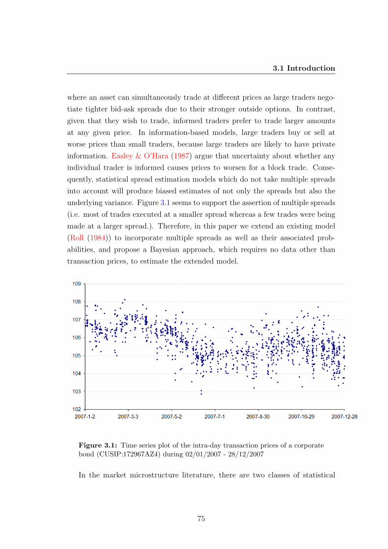
3.1 Introduction
where an asset can simultaneously trade at different prices as large traders nego-
tiate tighter bid-ask spreads due to their stronger outside options. In contrast,
given that they wish to trade, informed traders prefer to trade larger amounts
at any given price. In information-based models, large traders buy or sell at
worse prices than small traders, because large traders are likely to have private
information. Easley & O’Hara (1987) argue that uncertainty about whether any
individual trader is informed causes prices to worsen for a block trade. Conse-
quently, statistical spread estimation models which do not take multiple spreads
into account will produce biased estimates of not only the spreads but also the
underlying variance. Figure 3.1 seems to support the assertion of multiple spreads
(i.e. most of trades executed at a smaller spread whereas a few trades were being
made at a larger spread.). Therefore, in this paper we extend an existing model
(Roll (1984)) to incorporate multiple spreads as well as their associated prob-
abilities, and propose a Bayesian approach, which requires no data other than
transaction prices, to estimate the extended model.
Figure 3.1: Time series plot of the intra-day transaction prices of a corporatebond (CUSIP:172967AZ4) during 02/01/2007 - 28/12/2007
In the market microstructure literature, there are two classes of statistical
75

3.1 Introduction
models of estimating the effective bid-ask spread: the covariance model, and the
trade indicator model.
In the covariance models the spread measures are derived from the serial
covariance properties of transaction price changes. The first such model was de-
veloped by Roll (1984). By assuming an informationally efficient market and a
stationary probability distribution of observed price changes, the effective bid-ask
spread is inferred from the serial covariance of daily and weekly equity returns.
Choi et al. (1988) modify Roll’s estimator and introduce a serial correlation as-
sumption regarding transaction type. Stoll (1989) models the relation between
the quoted spread and the covariance estimate of the spread as a function of the
probability of a price reversal and the magnitude of a price reversal. The empir-
ical results imply that the average realized spread is less than the quoted spread.
George et al. (1991) show that positively autocorrelated time-varying expected
returns lead to downward biases in estimators of both the spread and its compo-
nents. They introduce an alternative approach based on the serial covariance of
the difference between transaction returns and returns calculated using bid prices
to adjust transaction returns for time-varying expected returns.
In the trade indicator models, the bid-ask spread is estimated as the coeffi-
cient of signed order flow in a price change regression. Glosten & Harris (1988)
applied this idea to separate the adverse selection spread component from the
one due to inventory costs, clearing fees, and/or monopoly profits. Their model
is estimated by integrating unobservable variables (underlying values and trade
directions) out of the conditional likelihood function and maximizing the uncon-
ditional likelihood function. Madhavan & Smidt (1991) develop a similar model
by explicitly modelling the learning process of the market maker. A reduced
form model and a measure of information asymmetry are estimated using Box-
Jenkins methods. Madhavan et al. (1997) develop and estimate a structural
model of price formation that decomposes intraday volatility into components
attributable to public information shocks and trading frictions. Both Madhavan
& Smidt (1991) and Madhavan et al. (1997) adopt trade classification procedure
to determine the trade directions. Huang & Stoll (1997) also construct a basic
trade indicator model which is estimated by GMM. They are able to observe in-
dicator variables and classify them for each size category. Ball & Chordia (2001)
76

3.1 Introduction
model the observed price as a discrete version of the sum of a permanent in-
formational component and the transient components arising out of the trading
mechanism. Since explicitly allowing for rounding onto the tick grid destroys the
Gaussian structure, they adopt Monte Carlo Markov Chain (MCMC) method to
estimate the models and to decide the best model specification. Recently, Has-
brouck (2004) suggested a Bayesian Gibbs approach by treating trade direction
as a latent variable and deriving a probability density for the sign of the trade,
and applied the approach to commodity futures transaction data.1
Our model belongs to the second category. Our purpose is to develop a par-
simonious but realistic model which does not have too many assumptions and
requires as few data to estimate as possible. Compared to Choi et al. (1988),
Stoll (1989), and George et al. (1991), our reduced-form model does not associate
price changes to transaction types, and thereby does not require data about quotes
and trade directions. Unlike Glosten & Harris (1988), Madhavan & Smidt (1991),
Madhavan et al. (1997), Huang & Stoll (1997), and Ball & Chordia (2001), we do
not intend to decompose the bid-ask spread into inventory cost and adverse selec-
tion components. Our model focuses on estimating the effective bid-ask spreads
as well as the underlying variance. In the original Roll model, it is not possible
to distinguish spreads of different magnitudes. The Roll measure is essentially a
weighted average of those spreads. We extend Roll’s model by adding an extra
parameter λ, the so-called ‘spread multiplier’, to separate different spreads. In
other words, we generalize Roll’s spread estimator (a scalar) to a vector of spreads
with associated probabilities. Different from Huang & Stoll (1997) where they
allow the components of the spread to explicitly depend on the trade size, our
extended model does not emphasize this link between the spread and the trade
size.
Our estimation procedure is based on a Bayesian Gibbs estimation method
proposed by Hasbrouck (2004). The trader direction is treated as a latent vari-
able which can be inferred from the transaction prices using a Bayesian trade
1Both Glosten & Harris (1988) and Madhavan & Smidt (1991) find strong evidence ofinformation asymmetry, whereas Huang & Stoll (1997) find a large order processing componentand smaller adverse selection and inventory components. Ball & Chordia (2001) focus ondiscreteness and find that for large stocks, most of the quoted spread is attributable to therounding of prices and the adverse selection component is small.
77

3.1 Introduction
classification method. Therefore, different from Madhavan & Smidt (1991) and
Madhavan et al. (1997), our model does not depend on a tick test to identify
trade directions. This estimation approach is very intuitive, and to some extent
similar to Huang & Stoll (1997) as we essentially integrate out the latent variables
numerically. We treat models with different values of λ as competitive models.
The value of λ is determined via a Bayesian model selection method, proposed
by Chib (1995).1
The simulation analysis shows that the model performs well when the un-
derlying volatility is low, and the difference between the inner and outer (half)
spreads is big compared to the underlying volatility. The empirical estimation
shows that our extended model fits the transaction data better than Roll’s model
(estimated using Method of Moments and Bayesian approaches).
We organize this chapter as follows. Section 2 presents the model specification
of the original Roll model, followed by the extended model. In Section 3, we
introduce the Bayesian model estimation and selection methodology, and the
details of the computational procedures. Simulation analysis is carried out in
Section 4 to assess the performance of the Bayesian estimators. An example of
an application to the actual transaction data is given in Section 5. Section 6
contains our conclusions.
1Bayes factors and various model selection criteria have been applied to compare financialmodels e.g. Osiewalski & Pipien (2004) and Deschamps (2011). In Ball & Chordia (2001), thechosen model is also determined by the Bayesian model selection method proposed by Chib(1995).
78

3.2 The Model
3.2 The Model
This section first gives a brief introduction to the basic Roll model. Based on
which, we present our extended model and discuss the key parameters.
3.2.1 The Roll Model
It has long been recognized that if trades fluctuate between bid and ask prices,
then observed price changes will be negatively autocorrelated. Roll (1984) uses
this property of transaction prices to derive an estimator of the bid-ask spread.
One advantage of his model is that it is based only on published transaction
prices.
In an efficient market the price dynamics may be stated as
mt = mt−1 + εt, (3.1)
pt = mt + sqt, (3.2)
where mt is the unobservable efficient price, pt is the transaction price observed
at time t, s is one-half the bid-ask spread, and the qt are trade direction indi-
cators, which take the values +1 for buy orders or −1 for sell orders with equal
probability.
The changes in transaction prices between two successive trades is
pt − pt−1 = mt + sqt − (mt−1 + sqt−1), (3.3)
∆pt = s∆qt + εt. (3.4)
Thus,
Cov(∆pt,∆pt−1) = E[∆qt∆qt−1s2] + E[∆qtεt−1s]
+ E[∆qt−1εts] + E[εtεt−1],(3.5)
where Cov(∆pt,∆pt−1) is the first-order autocovariance of the price changes.
79

3.2 The Model
In deriving the Method of Moments estimator Roll (1984) makes several as-
sumptions:
1. Successive transaction types are independent. Thus,
E[qtqt−1] = 0.
2. The half-spread s is constant.
3. Order flows do not contain information about future fundamental price
changes. Thus,
E[∆qt−1εt] = 0.
4. Changes in fundamental value cannot predict order flows:
E[∆qtεt−1] = 0.
5. The innovations in the fundamental price process reflect public information
and are assumed to be independent. Therefore,
E[εtεt−1] = 0.
Table 3.1: Joint probabilities of consecutive price changes
4qt−1
-2 0 +2
-2 0 18
18
4qt 0 18
14
18
+2 18
18
0
Then, from the joint probabilities in Table 3.1, Equation 3.5, and the assump-
tions, we obtain
Cov(∆pt,∆pt−1) = −s2. (3.6)
80
3.2 The Model
This gives Roll’s Method of Moments spread estimator
s =√−Cov(∆pt,∆pt−1). (3.7)
If the innovations in the efficient price process are assumed to follow a normal
distribution with mean 0 and constant variance σ2ε , the Method of Moments
variance estimator is
σ2ε = V ar(∆pt)− s2V ar(∆qt) = V ar(∆pt)− 2s2. (3.8)
However, Roll’s method of moments spread estimator has performed poorly,
generating undefined spread estimates almost half of the time when applied to
daily transaction data on equities [Harris (1990)]. In particular, Roll’s model is
not able to identify the multiple spreads with different magnitudes. The estimator
is only a scalar which is, essentially, a weighted average of those spreads. However,
several refinements of the Roll’s model are possible. Our extended model, which
will be introduced in the next section, provides a richer structure, and does not
produce undefined spread estimates.
3.2.2 The Extended Model
The fact that trades are sometimes executed either inside or outside the posted
bid and ask indicates that sometimes the posted spread may not represent the
transaction cost that investors can expect. This motivates our extended Roll
model aiming at separating spreads with two different magnitudes.
In our model the trade direction indicators qt are generalised as follow:
qt ∈ −λ,−1,+1,+λ, (3.9)
where λ is the so-called ‘spread multiplier’ which is used to distinguish different
spreads. Thus, for expositional ease, we define λ ∈ [1,+∞)1. λ 6= 1 implies
1Equivalently, we can define λ ∈ (0, 1]. For computational ease, we choose to use λ ∈ (0, 1]later in the estimation.
81
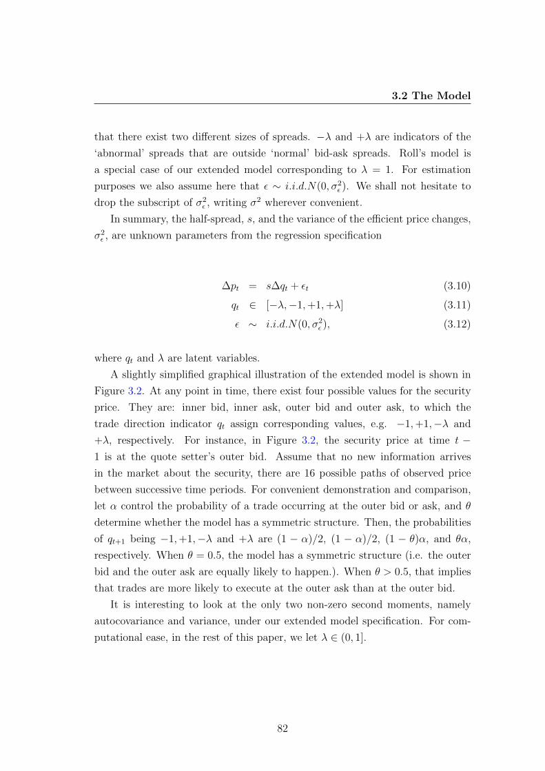
3.2 The Model
that there exist two different sizes of spreads. −λ and +λ are indicators of the
‘abnormal’ spreads that are outside ‘normal’ bid-ask spreads. Roll’s model is
a special case of our extended model corresponding to λ = 1. For estimation
purposes we also assume here that ε ∼ i.i.d.N(0, σ2ε ). We shall not hesitate to
drop the subscript of σ2ε , writing σ2 wherever convenient.
In summary, the half-spread, s, and the variance of the efficient price changes,
σ2ε , are unknown parameters from the regression specification
∆pt = s∆qt + εt (3.10)
qt ∈ [−λ,−1,+1,+λ] (3.11)
ε ∼ i.i.d.N(0, σ2ε ), (3.12)
where qt and λ are latent variables.
A slightly simplified graphical illustration of the extended model is shown in
Figure 3.2. At any point in time, there exist four possible values for the security
price. They are: inner bid, inner ask, outer bid and outer ask, to which the
trade direction indicator qt assign corresponding values, e.g. −1,+1,−λ and
+λ, respectively. For instance, in Figure 3.2, the security price at time t −1 is at the quote setter’s outer bid. Assume that no new information arrives
in the market about the security, there are 16 possible paths of observed price
between successive time periods. For convenient demonstration and comparison,
let α control the probability of a trade occurring at the outer bid or ask, and θ
determine whether the model has a symmetric structure. Then, the probabilities
of qt+1 being −1,+1,−λ and +λ are (1 − α)/2, (1 − α)/2, (1 − θ)α, and θα,
respectively. When θ = 0.5, the model has a symmetric structure (i.e. the outer
bid and the outer ask are equally likely to happen.). When θ > 0.5, that implies
that trades are more likely to execute at the outer ask than at the outer bid.
It is interesting to look at the only two non-zero second moments, namely
autocovariance and variance, under our extended model specification. For com-
putational ease, in the rest of this paper, we let λ ∈ (0, 1].
82
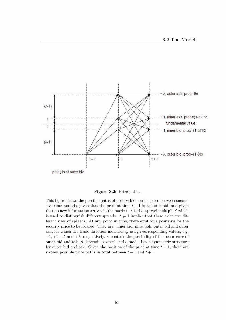
3.2 The Model
Figure 3.2: Price paths.
This figure shows the possible paths of observable market price between succes-sive time periods, given that the price at time t − 1 is at outer bid, and giventhat no new information arrives in the market. λ is the ‘spread multiplier’ whichis used to distinguish different spreads. λ 6= 1 implies that there exist two dif-ferent sizes of spreads. At any point in time, there exist four positions for thesecurity price to be located. They are: inner bid, inner ask, outer bid and outerask, for which the trade direction indicator qt assign corresponding values, e.g.−1,+1,−λ and +λ, respectively. α controls the possibility of the occurrence ofouter bid and ask. θ determines whether the model has a symmetric structurefor outer bid and ask. Given the position of the price at time t − 1, there aresixteen possible price paths in total between t− 1 and t+ 1.
83
3.2 The Model
Using the probabilities of different prices as just described, we have,
Cov(∆pt,∆pt−1) = − s2(1− α)3 − s2α2(1− α)[λ2(1 + 4θ − 4θ2) + 1]
− s2(1− α)2α(λ2 + 2)− 4s2α3λ2θ(1− θ), (3.13)
and
V ar(∆pt) = σ2ε+s
2[8λ2(θ−θ2)α2+2(λ2+1)α2(1−α)+2(λ2+2)(1−α)2α+2(1−α)3].
(3.14)
Assuming that s = 1, θ = 0.5, and λ 6= 1, Roll’s spread estimator will be biased
as shown in Figure 3.3. The bias increases while α increases. That is, the bias
increases as the probability of existence of the outer spread increases. The bias
also increases while λ decreases, as Roll’s spread estimator is a weighted average
of the inner and outer spreads. Roll’s variance estimator is also biased as shown in
Figure 3.4. The bias increases as α increases. This is because that the estimator
mistakenly treats some of the transitory effect due to big spreads as the permanent
effect. The bias again increases while λ decreases. This is due to the fact that
the outer spread increases while λ decreases. That is, if our extended model is
the true data generating process, Roll’s measure will be biased.
84

3.2 The Model
Figure 3.3: Plot of autocovariance I
This figure provides the autocovariances calculated under the extended model.s is the half-spread. λ is the ‘spread multiplier’ which is used to distinguishdifferent spreads. λ 6= 1 means that there exist two different sizes of spreads.α controls the possibility of the occurrence of outer bid and ask. θ determineswhether the model has a symmetric structure for outer bid and ask. Assumes = 1 and θ = 0.5. Different lines in this figure represent autocovariances as afunction of λ for a few values of α. Autocovariance under the extended modelis computed asCov(∆pt,∆pt−1) = −s2(1 − α)3 − s2α2(1 − α)[λ2(1 + 4θ − 4θ2) + 1] − s2(1 −α)2α(λ2 + 2)− 4s2α3λ2θ(1− θ).
85
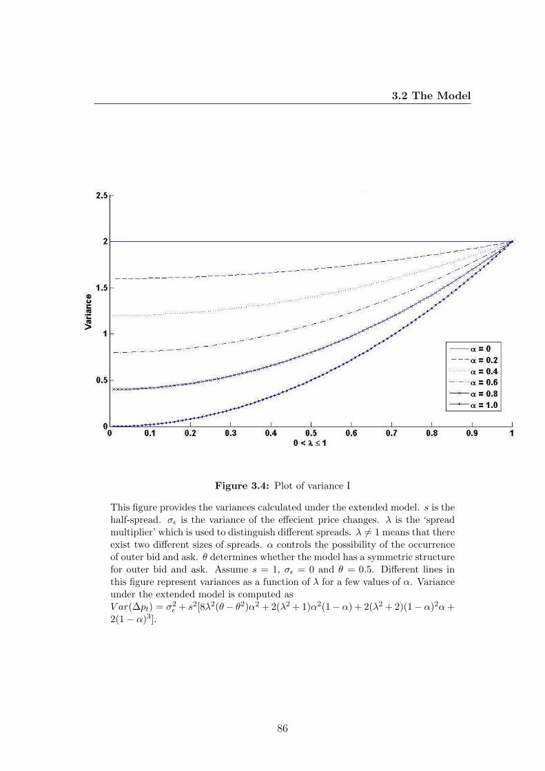
3.2 The Model
Figure 3.4: Plot of variance I
This figure provides the variances calculated under the extended model. s is thehalf-spread. σε is the variance of the effecient price changes. λ is the ‘spreadmultiplier’ which is used to distinguish different spreads. λ 6= 1 means that thereexist two different sizes of spreads. α controls the possibility of the occurrenceof outer bid and ask. θ determines whether the model has a symmetric structurefor outer bid and ask. Assume s = 1, σε = 0 and θ = 0.5. Different lines inthis figure represent variances as a function of λ for a few values of α. Varianceunder the extended model is computed asV ar(∆pt) = σ2
ε + s2[8λ2(θ− θ2)α2 + 2(λ2 + 1)α2(1− α) + 2(λ2 + 2)(1− α)2α+2(1− α)3].
86

3.3 The Model Estimation and Selection
3.3 The Model Estimation and Selection
The latent variables in the extended model are the trade direction indicators qt
and the spread multiplier λ. Since integrating out the latent variables is cum-
bersome, there is no attractive closed-form solution for the likelihood function.
Moreover, it is difficult to compute the higher moments, using GMM estima-
tion, which are needed in order to estimate the extended model. Therefore, our
extended model is estimated via a Bayesian approach proposed by Hasbrouck
(2004). More precisely, the model parameters, the half-spread s and the under-
lying variance σ2ε , are estimated using a Markov chain Monte Carlo (MCMC)
method, the Gibbs sampler. Then, we treat models with different specifications
of λ as competitive models. The best model is determined via a Bayesian model
selection method which is introduced by Chib (1995). The advantage of this
method is that it is also based on the Gibbs outputs.1 The most appealing mo-
tivation for the use of the Bayesian approach lies in the fact that the role of the
latent variables in the estimation can be intuitively understood. In the following,
we describe the parameter estimation procedure in detail, followed by the model
selection method.
3.3.1 The Bayesian Estimation Procedure
The extended model has two parameters s, σε, and T latent variables q =
(q1, q2, . . . , qT ) given the value of λ. We estimate the model parameters via a
Bayesian approach, using the Gibbs sampler. That is, given a known sequence of
observations p = (p1, p2, . . . , pT ), we estimate s and σε under mean squared error
risk rule by taking the mean of the posterior distributions of s and σε for fixed
λ.2
Gibbs sampling is a technique for generating random variables from a marginal
distribution indirectly, without having to calculate the joint density. As a Markov
1This approach shares some similarities with the Expectation-Maximization (EM) algorithmwhich is also an iterative method for finding maximum likelihood estimates in statistical models,which the model has some latent variables.
2Using the MSE as risk, the Bayes estimate of the unknown parameter is simply the meanof the posterior distribution.
87

3.3 The Model Estimation and Selection
chain Monte Carlo method, the Gibbs sampler generates sample values from the
distribution of each variable in turn, conditional on the current values of the other
variables.
Gibbs sampling is, essentially, an iterative procedure. An iteration is generally
termed a “sweep”. Initially, i.e., j = 0, for fixed λ the parameters and the latent
variables are set to any values, where tick test results can be used as initial values
for q, and the Method of Moments estimates for s and σε. Denote these initial
values (s(0), σ(0)ε , q(0)), where q(0) = (q
(0)1 , q
(0)2 , . . . , q
(0)T ).
The steps in the first sweep (j = 1) given λ and p are:
1. Draw s(1) from fs(s|σ(0)ε , q(0), p, λ),
2. Draw σ(1)ε from fσε(σε|s(1), q(0), p, λ),
3. Draw q(1) from fq(q|s(1), σ(1)ε , p, λ),
where f(·|·) is the complete conditional density.
Similarly, draws for q(1)t for t = 1, . . . , T are made sequentially using the Gibbs
sampler. The steps in the first sweep (j = 1) are then:
1. Draw q(1)1 from fq(q1|s(1), σ
(1)ε , p, λ, q
(0)2 , q
(0)3 , · · · , q(0)
T ),
2. Draw q(1)2 from fq(q2|s(1), σ
(1)ε , p, λ, q
(1)1 , q
(0)3 , · · · , q(0)
T ),
... · · ·
T. Draw q(1)T from fq(qT |s(1), σ
(1)ε , p, λ, q
(1)1 , q
(1)2 , · · · , q(1)
T−1).
Note that, all parameters and latent variables except for the component being
drawn are taken as given.
The next iteration starts with a draw of s(2) conditional on σ(1)ε , q(1), p and
λ. Repeating this n times, we generate a sequence of draws (s(j), σ(j)ε , q(j)) for
j = 1, . . . , n, where q(j) = (q(j)1 , q
(j)2 , . . . , q
(j)T ). The Gibbs principle ensures that
the limiting distribution of the nth draw (as n→∞) is F (s, σε, q|p, λ). The lim-
iting draw for any parameter is distributed in accordance with the corresponding
marginal posterior, i.e., the limiting density of s(n) is fs(s|p, λ). Given some
continuous function of the model parameters, h(s, σε, q) and a set of parameter
88
3.3 The Model Estimation and Selection
draws, (s(j), σ(j)ε , q(j) : j = 1, . . . , n), the corresponding sequence (h(s(j), σ
(j)ε , q(j) :
j = 1, . . . , n)) generally has a limiting distribution for h(s, σε, q).
The consistent estimates of population parameters θ = (s, σε) are given by the
posterior mean Eθ|p,λ(θ). If one is interested in some statistic g(θ), then Eθ|p,λg(θ)
is a consistent estimate of g(θ).
3.3.2 The Bayesian Model Selection
Suppose we have K models Mk (k = 1, 2, . . . , K), given the model-specific pa-
rameter vector θk. Our prior information on these models can be used to assign
each of them a prior probability π(θk|Mk). A data set y = (y1, y2, . . . , yn) is used
to update these prior probabilities. The marginal likelihood m(y|Mk) of y under
model Mk is defined by
m(y|Mk) =
∫f(y|θk,Mk)π(θk|Mk)dθk, (3.15)
where f(y|θk,Mk) is the probability density of y given the value of θk, or the
likelihood function of θk.
The Bayes factor is defined as the log of the ratio of the marginal likelihoods
for any two competing models k and l:
Bkl = ln
(m(y|Mk)
m(y|Ml)
). (3.16)
The preferred model is the one with the highest marginal likelihood. Therefore,
evaluating the marginal likelihood is the key to Bayesian model selection.
Using the Basic Marginal Likelihood Identity (BMI), the marginal likelihood
can be written as
m(y) =f(y|θ)π(θ)
π(θ|y), (3.17)
where the numerator is the product of the likelihood and the prior, and the
denominator is the posterior density. Conveniently, it can be expressed in a
89

3.3 The Model Estimation and Selection
logarithmic scale as
lnm(y) = ln f(y|θ)− lnπ(θ|y)
π(θ), (3.18)
where the first term measures how well the model fits the data given the most
probable parameter values, and the second term penalizes the model according
to its complexity. Hence, the marginal likelihood automatically incorporates a
tradeoff between model fit and its complexity.
The marginal likelihood can be evaluated from the Gibbs output, generated
during the simulation stage, as suggested by Chib (1995).
Let z denote latent data, and suppose that for a given set of vector blocks
θ = (θ1, θ2, . . . , θB), the Gibbs sampling algorithm is applied to the set of (B +
1) complete conditional densities, π(θr|y, θs(s 6= r), z)Br=1 and π(z|y, θ). The
goal is to compute the marginal likelihood m(y) from the output θ(j), z(j)nj=1
obtained from these full conditional densities. In some situations, the density
f(y|θ) =∫f(y, z|θ)dz is not available in closed form, however, the likelihood
f(y|θ, z) is. The marginal likelihood m(y) in this situation has the form
m(y) =f(y|θ, z)π(θ, z)
π(θ, z|y), (3.19)
where the likelihood f(y|θ, z), the prior π(θ, z), and the multivariate posterior
density π(θ, z|y) can be evaluated at the selected high density point (θ∗, z∗) (e.g.
the mode of the posterior density derived from the Gibbs sampler). When esti-
mating π(θ, z|y), z can be treated as an additional block, e.g. z ≡ θB+1. Evalu-
ating at a particular point θ∗, we have
lnm(y) = ln f(y|θ∗) + ln π(θ∗)− lnπ(θ∗|y). (3.20)
The posterior density at the selected high density point is given by
π(θ∗|y) = π(θ∗1|y)× π(θ∗2|y, θ∗1)× . . .× π(θ∗B+1|y, θ∗1, . . . , θ∗B), (3.21)
90
3.3 The Model Estimation and Selection
where the first term on the right hand side is the marginal ordinate, which
can be estimated from the draws of the initial Gibbs sampling, e.g. π(θ∗1|y) =
n−1∑n
j=1 π(θ∗1|y, θ(j)s (1 < s ≤ B + 1)), and the rest of the terms are the reduced
conditional ordinates with the typical form of π(θ∗r |y, θ∗1, θ∗2, . . . , θ∗r−1), which are
given by
∫π(θ∗r |y, θ∗1, θ∗2, . . . , θ∗r−1, θr+1, . . . , θB)dπ(θr+1, . . . , θB|y, θ∗1, θ∗2, . . . , θ∗r−1). (3.22)
To estimate the above integral, continue the sampling with the complete con-
ditional densities of θr, θr+1, . . . , θB+1, where in each of these full conditional
densities, θs is set equal to θ∗s , (s ≤ r − 1). If the draws from the reduced com-
plete conditional Gibbs sampling are denoted by θ(g)r , θ
(g)r+1, . . . , θ
(g)B+1, then an
estimate of (3.22) is
π(θ∗r |y, θ∗s(s < r)) = n−1
n∑g=1
π(θ∗r |y, θ∗1, θ∗2, . . . , θ∗r−1, θ(g)l (l > r)). (3.23)
Therefore, an estimate of the posterior density is
π(θ∗1|y)ΠBr=2π(θ∗r |y, θ∗s(s < r))π(z∗|y, θ∗s(s < B + 1)). (3.24)
The log of the marginal likelihood is
ln m(y) = ln f(y|θ∗, z∗) + ln π(θ∗, z∗)− ln π(θ∗1|y)
−B∑r=2
ln π(θ∗r |y, θ∗s(s < r))− lnπ(z∗|y, θ∗s(s < B + 1)).
(3.25)
In our situation for θ = (s, σε, q), where we suppress λ for convenience, Gibbs
sampling is applied to the complete conditional densities
π(θ1|y, θ2, z) = fs(s|p, σε, q), (3.26)
91
3.3 The Model Estimation and Selection
π(θ2|y, θ1, z) = fσε(σε|p, s, q), (3.27)
π(z|y, θ) = fq(q|p, s, σε). (3.28)
The goal is to estimate the posterior ordinate f(s∗, σ∗ε , q∗|p), which is now
expressed as fs(s∗|p)fσ∗
ε(σ∗ε |p, s∗)fq(q∗|p, s∗, σ∗ε ). The first term, fs(s
∗|p), can be
estimated by taking the average of the full conditional density with the posterior
draws of (σε, q), leading to the estimate
fs(s∗|p) = n−1
n∑j=1
fs(s∗|p, σ(j)
ε , q(j)). (3.29)
Continue sampling for an additional n iterations with the complete conditional
densities fσε(σε|p, s, q) and fq(q|p, s, σε), where in each of these densities, s is set
equal to s∗. It can be shown that the draws q(g) from this round of iterations
follow the density fq(q|p, s∗), as required. Therefore,
ˆfσ∗ε(σ∗ε |p, s∗) = n−1
n∑g=1
fσ∗ε(σ∗ε |p, s∗, q(g)). (3.30)
Substituting the density estimates into (3.25) yields the following estimate of the
marginal likelihood:
ln m(p) = ln f(p|s∗, σ∗ε , q∗)+ln f(s∗, σ∗ε , q∗)−ln fs(s
∗|p)−ln ˆfσ∗ε(σ∗ε |p, s∗)−ln fq(q
∗|p, s∗, σ∗ε ),(3.31)
where f(s∗, σ∗ε , q∗) = fs(s
∗)fσε(σ∗ε )fq(q
∗) which is the product of the prior densities
of s, σε and q evaluated at s∗, σ∗ε and q∗.
The performance of the Gibbs sampler and an example of the application of
the Bayesian model estimation and selection techniques are illustrated in the next
two sections.
92

3.4 Simulation Analysis
3.4 Simulation Analysis
The performance of the Bayesian estimators may be illustrated by considering
simulated samples under three different specifications. The specifications corre-
spond to typical situations in the marketplace. Assume trades can execute at two
bid-ask spreads, e.g. the inner spread and outer spread.
First scenario, trades execute at inner spread and outer spread with equal
probabilities. That means p(q = ±λ) = p(q = ±1), that is, p(q = λ) = p(q =
−λ) = p(q = 1) = p(q = −1) = 0.25 in Figure 3.5, where p(·) is the probability
of the trade direction indicator q.
Figure 3.5: Joint posteriors of half spread s and variance σ2 I
This figure provides the joint posteriors of half spread s and variance σ2, givenλ for four simulated series of length 300 with probabilities p(q = +λ) = 0.25,p(q = +1) = 0.25, p(q = −1) = 0.25, p(q = −λ) = 0.25: Top-left panel: s = 8,σ2 = 1, λ = 0.25; Top-right panel: s = 8, σ2 = 16, λ = 0.25; Bottom-left panel:s = 4, σ2 = 1, λ = 0.5; Bottom-right panel: s = 4, σ2 = 16, λ = 0.5.
Second scenario, most of trades are executed at the outer spread, while a few
orders execute at the inner spread. In other words, p(q = ±λ) > p(q = ±1), say,
p(q = λ) = p(q = −λ) = 0.40 and p(q = 1) = p(q = −1) = 0.10 in Figure 3.6.
93
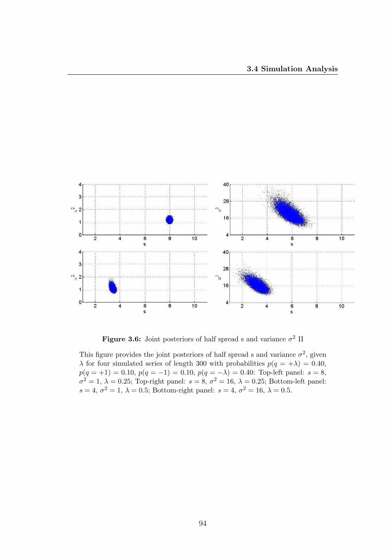
3.4 Simulation Analysis
Figure 3.6: Joint posteriors of half spread s and variance σ2 II
This figure provides the joint posteriors of half spread s and variance σ2, givenλ for four simulated series of length 300 with probabilities p(q = +λ) = 0.40,p(q = +1) = 0.10, p(q = −1) = 0.10, p(q = −λ) = 0.40: Top-left panel: s = 8,σ2 = 1, λ = 0.25; Top-right panel: s = 8, σ2 = 16, λ = 0.25; Bottom-left panel:s = 4, σ2 = 1, λ = 0.5; Bottom-right panel: s = 4, σ2 = 16, λ = 0.5.
94
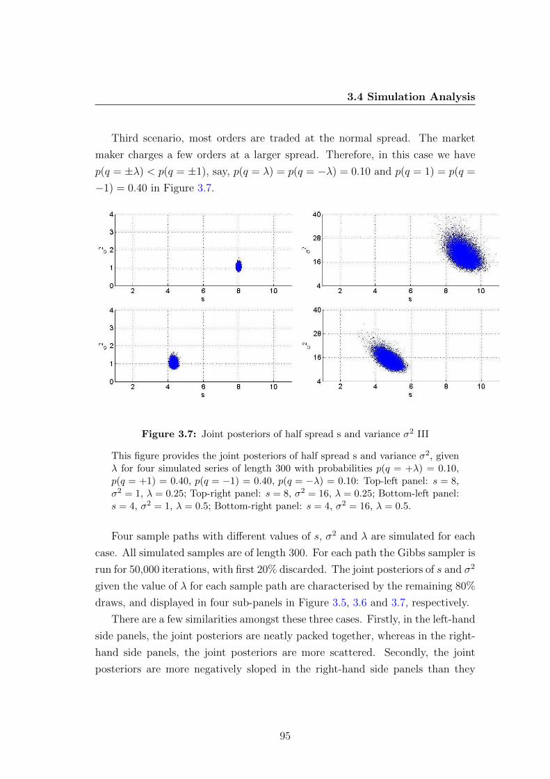
3.4 Simulation Analysis
Third scenario, most orders are traded at the normal spread. The market
maker charges a few orders at a larger spread. Therefore, in this case we have
p(q = ±λ) < p(q = ±1), say, p(q = λ) = p(q = −λ) = 0.10 and p(q = 1) = p(q =
−1) = 0.40 in Figure 3.7.
Figure 3.7: Joint posteriors of half spread s and variance σ2 III
This figure provides the joint posteriors of half spread s and variance σ2, givenλ for four simulated series of length 300 with probabilities p(q = +λ) = 0.10,p(q = +1) = 0.40, p(q = −1) = 0.40, p(q = −λ) = 0.10: Top-left panel: s = 8,σ2 = 1, λ = 0.25; Top-right panel: s = 8, σ2 = 16, λ = 0.25; Bottom-left panel:s = 4, σ2 = 1, λ = 0.5; Bottom-right panel: s = 4, σ2 = 16, λ = 0.5.
Four sample paths with different values of s, σ2 and λ are simulated for each
case. All simulated samples are of length 300. For each path the Gibbs sampler is
run for 50,000 iterations, with first 20% discarded. The joint posteriors of s and σ2
given the value of λ for each sample path are characterised by the remaining 80%
draws, and displayed in four sub-panels in Figure 3.5, 3.6 and 3.7, respectively.
There are a few similarities amongst these three cases. Firstly, in the left-hand
side panels, the joint posteriors are neatly packed together, whereas in the right-
hand side panels, the joint posteriors are more scattered. Secondly, the joint
posteriors are more negatively sloped in the right-hand side panels than they
95
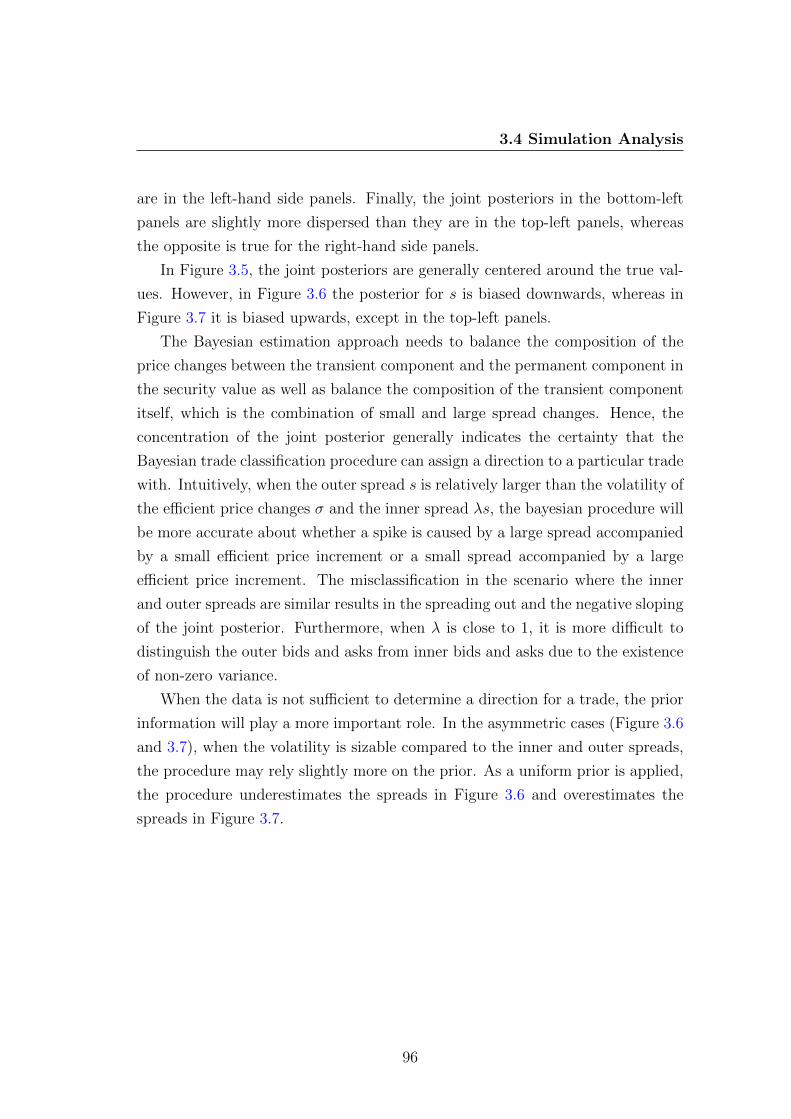
3.4 Simulation Analysis
are in the left-hand side panels. Finally, the joint posteriors in the bottom-left
panels are slightly more dispersed than they are in the top-left panels, whereas
the opposite is true for the right-hand side panels.
In Figure 3.5, the joint posteriors are generally centered around the true val-
ues. However, in Figure 3.6 the posterior for s is biased downwards, whereas in
Figure 3.7 it is biased upwards, except in the top-left panels.
The Bayesian estimation approach needs to balance the composition of the
price changes between the transient component and the permanent component in
the security value as well as balance the composition of the transient component
itself, which is the combination of small and large spread changes. Hence, the
concentration of the joint posterior generally indicates the certainty that the
Bayesian trade classification procedure can assign a direction to a particular trade
with. Intuitively, when the outer spread s is relatively larger than the volatility of
the efficient price changes σ and the inner spread λs, the bayesian procedure will
be more accurate about whether a spike is caused by a large spread accompanied
by a small efficient price increment or a small spread accompanied by a large
efficient price increment. The misclassification in the scenario where the inner
and outer spreads are similar results in the spreading out and the negative sloping
of the joint posterior. Furthermore, when λ is close to 1, it is more difficult to
distinguish the outer bids and asks from inner bids and asks due to the existence
of non-zero variance.
When the data is not sufficient to determine a direction for a trade, the prior
information will play a more important role. In the asymmetric cases (Figure 3.6
and 3.7), when the volatility is sizable compared to the inner and outer spreads,
the procedure may rely slightly more on the prior. As a uniform prior is applied,
the procedure underestimates the spreads in Figure 3.6 and overestimates the
spreads in Figure 3.7.
96

3.5 Empirical Application
3.5 Empirical Application
The extended model is applied to a time series of intra-day bond prices, as the
data in Figure 3.1 suggests that the extended model might be an appropriate
underlying model. Table 3.2 summarizes the basic information about the bond
and the descriptive statistics of the sample.
The Gibbs sampler is run for 10,000 iterations, with first 20% discarded.
Our results for the data are presented in Table 3.3. The Method of Moments
estimate for the spread s is about three standard deviations bigger than the
Bayesian estimate under Roll’s model. The Bayesian estimate of the spread s
under Roll’s model and the Method of Moments estimate are in between the
estimated inner and outer spreads (the grand average of the estimated inner and
outer spreads is 0.4762), suggesting that Roll’s spread measures estimated using
both the classic and Bayesian approaches are essentially some weighted averages
of the two spreads. For the variance σ2, the Method of Moments estimate is five
standard deviations smaller than the Bayesian estimate under Roll’s model, but
sixteen standard deviations bigger than the Bayesian estimate under the extended
model. The estimated log marginal likelihood is equal to -1182.8434 for Roll’s
model. By contrast with the extended model, the maximum of the estimated log
marginal likelihood is equal to -326.5221 at λ = 0.13. Therefore, the extended
model fits the data better than the original Roll’s model.
Additionally, the posterior median mt as the estimate of the efficient price mt
together with the estimated inner and outer bid-ask bounces, defined as mt ± sand mt± sλ respectively, are also shown in Figure 3.8. It is clear from the figure
that trades executed with different transaction costs are distributed between the
corresponding estimated bid-ask spreads. Furthermore, the estimates of α and
θ are 34% and 53%, respectively. The estimate of α indicates that 66% of the
trades happened at the inner spread and the estimate of θ supports a symmetric
structure (i.e. the outer bid and the outer ask are equally likely to happen.).
The estimated efficient price changes 4m under the extended model exhibits less
serial correlation than they do under Roll’s model, as shown in Table 3.4. This
implies that the permanent component of the transaction prices, which reflect
97
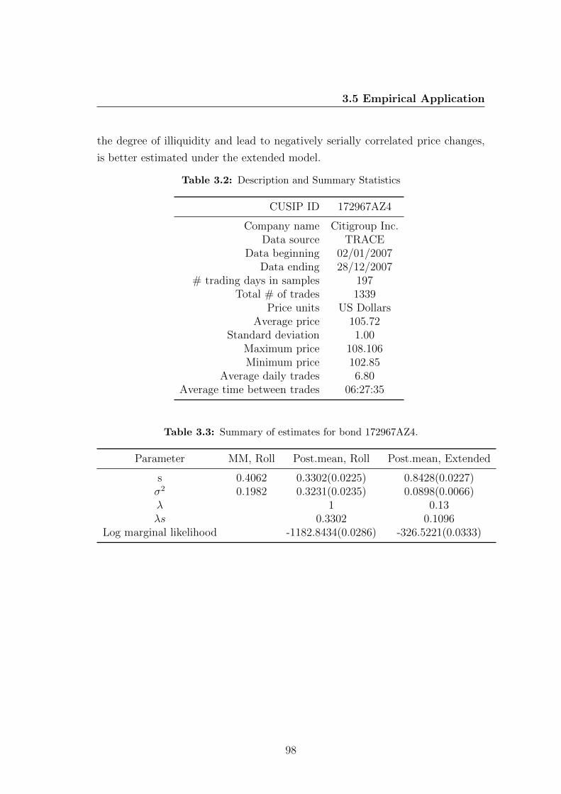
3.5 Empirical Application
the degree of illiquidity and lead to negatively serially correlated price changes,
is better estimated under the extended model.
Table 3.2: Description and Summary Statistics
CUSIP ID 172967AZ4
Company name Citigroup Inc.Data source TRACE
Data beginning 02/01/2007Data ending 28/12/2007
# trading days in samples 197Total # of trades 1339
Price units US DollarsAverage price 105.72
Standard deviation 1.00Maximum price 108.106Minimum price 102.85
Average daily trades 6.80Average time between trades 06:27:35
Table 3.3: Summary of estimates for bond 172967AZ4.
Parameter MM, Roll Post.mean, Roll Post.mean, Extended
s 0.4062 0.3302(0.0225) 0.8428(0.0227)σ2 0.1982 0.3231(0.0235) 0.0898(0.0066)λ 1 0.13λs 0.3302 0.1096
Log marginal likelihood -1182.8434(0.0286) -326.5221(0.0333)
98

3.5 Empirical Application
Figure 3.8: Time series plot of transaction prices with estimated bid-askbounces
Table 3.4: Serial correlation of 4m.
Lag Roll Extended
1 -0.1646 -0.06232 -0.1186 -0.03313 -0.1323 -0.08934 -0.0786 -0.08145 0.0132 -0.06896 0.0295 0.00597 -0.0153 -0.0138 0.0074 -0.04249 0.0046 -0.0311
10 -0.0056 0.0269
99

3.6 Conclusions
3.6 Conclusions
In this paper we extend the Roll model to allow trades to be executed at two
different spreads with associated probabilities. The parameters of the extended
model are determined via a Bayesian approach, based on only transaction data. A
numerical example based on a set of corporate bond transaction data shows that
the extended model fits the data better. The estimated efficient price changes
under the extended model exhibits less serial correlation than those under Roll’s
model. The new model together with the model estimation and selection proce-
dures offers an alternative way to estimate the effective bid-ask spread and the
underlying variance.
100
Chapter 4
Non-default Yield Spread and
Illiquidity of Corporate Bonds
4.1 Introduction
During the recent financial crisis, corporate yield spreads widened dramatically.
Spreads were much larger than can be explained by expected losses arising from
default.1 The objective of this study is to understand that whether time se-
ries and cross-sectional variations of non-default yield spreads can be explained
by liquidity, and in particular, why bonds issued by a single company exhibit
heterogeneous levels of liquidity and liquidity premia.
Recognizing that a reasonable method to accurately extract the non-default
component of yield spreads is essential to our task, we follow Longstaff et al.
(2005) to compute the fundamental value of a corporate bond, as if it is perfectly
liquid, by using the information from credit default swaps. To this point, the
difference between our method and the one by Longstaff et al. (2005) is that the
latter uses a reduced-form approach which includes both default and liquidity
yield processes to price corporate bonds and credit default swaps simultaneously,
while we adopt a non-parametric approach to extract default intensities from
1See, for example, Bao et al. (2011) and Dick-Nielsen et al. (2012).
101
4.1 Introduction
credit default swap spreads of the same name as the bond, and then utilize the
default intensities to obtain the fundamental value of the bond which is the price
when the market is perfectly liquid. Our approach is capable to generate flexible
default term structures and thus avoids the misspecification problem of reduced-
form models.
Bid-ask spreads have been widely used as a measure of illiquidity in the litera-
ture.1 We are interested in both the level of illiquidity (the transitory component)
of the bonds and the liquidity premium (the permanent component) embedded
in bond yields.2 Order flow spread models are capable of estimating both the two
components. However, Roll’s model is clearly misspecified when applied to our
transaction data which have a non-constant transitory component, and the other
models with a richer structure require more detailed data (e.g. quotes or trade
directions) which are difficult to obtain for corporate bonds as they are traded in
OTC markets.
Therefore, our next task is to develop a parsimonious model which has a
reasonably rich structure and does not require extra data to estimate. We de-
veloped two competing models based on the original Roll model. The first one
is the model developed in the previous chapter which allows two different mag-
nitudes of bid-ask spreads with associated probabilities. The model is estimated
via a Bayesian approach. The second one is a Kalman Filter model which allows
the transitory component to vary over time and take continuous values. Com-
putationally, the second model is preferred since it works more efficiently when
applied to a relatively large data set.
A second difference between this study and previous studies on bond illiquid-
ity is that the latter examine raw transactions data, while we apply our extended
Roll model to the non-default price residuals which are calculated by subtracting
the corporate bond market prices from the theoretical fundamental values implied
from the credit default swap spreads. Therefore, our approach essentially decom-
poses the non-default price residuals into a transitory component which arises
from the illiquidity of the market and a permanent component which reflects
1See, for example, Bessembinder & Maxwell (2008), Edwards & Piwowar (2007) and Gold-stein et al. (2007).
2The liquidity premium in bond yields does not violate market efficiency, but simply reflectsthe rational response by the investors when taking into account the illiquidity of the asset.
102
4.1 Introduction
public information including information about future bond liquidity. Our mea-
sure of illiquidity is derived from the transitory component, which is supposed
to be orthogonal to the fundamental value. The permanent component of the
non-default price residuals can be expressed in terms of yield as non-default yield
spreads. Longstaff et al. (2005) find that non-default yield spreads are strongly
related to bond-specific illiquidity. Ericsson & Renault (2006) find evidence of a
positive correlation between illiquidity and default components of yield spreads.
However, they did not distinguish non-default yield spreads from transitory ef-
fects. Chen et al. (2007) find that more illiquid bonds earn higher yield spreads.
As they use over 4000 corporate bonds to cover the universe of corporate bond
market, they could not make use of the information in credit default swap market.
This leads to the third and final difference between our study and other pa-
pers related to the liquidity of corporate bond markets. The latter concentrate
on either developing illiquidity measures and associating them to bond charac-
teristics which are known to be related to bond illiquidity or trying to explain
the unexplained yield spread or return as liquidity premia. In contrast, our study
focuses on understanding time series and cross-sectional variations in both illiq-
uidity and liquidity premia of bonds issued by a single corporation. De Jong
& Driessen (2007) show that liquidity risk is a pricing factor for the expected
returns on corporate bonds, and the credit spread puzzle can be explained by
the associated liquidity premia. Bao et al. (2011) uses their bond-level illiquidity
measure to explain individual bond yield spreads. Their results suggest that for
high-rated corporate bonds, the sudden increase in illiquidity during the crisis
was the dominating factor in driving up yield spreads. By developing a new illiq-
uidity measure, Dick-Nielsen et al. (2012) analyze the liquidity components of
corporate bond spreads during 2005-2009. They find that the spread contribu-
tion from illiquidity increased dramatically with the onset of the subprime crisis.
The increase was slow and persistent for high-rated bonds. Our analysis shows
that before the crisis (before July 2007) and during the crisis (from July 2007 to
June 2009), the non-default spread accounted for about 80% and 48% of the yield
spreads on average, respectively. The proportion dropped to around 23% after
the crisis (after June 2009) as a result of the emergency liquidity supply from the
U.S. Treasury.
103

4.1 Introduction
Our study also sheds light on how the common and idiosyncratic factors af-
fect bond illiquidity and non-default yield spreads. By analyzing the variations
in both our illiquidity measure and the estimated non-default yield spread dur-
ing 2006 - 2010, our results show that the illiquidity measure has a nonlinear
positive relationship with time-to-maturities, and is negatively correlated with
issue sizes and the trading activity measures. Both fundamental volatilities and
CDS spreads are positively correlated with the illiquidity measure. The common
factors such as fundamental volatilities and CDS spreads can explain 17.57% of
the variations in the illiquidity measure. Adding the idiosyncratic factors such
as time-to-maturities, issue sizes, and the trading activity measures improves the
R2 by roughly about 3%.
The regression results of non-default yield spreads show that non-default yield
spreads are positively correlated with our illiquidity measure. Adding the illiq-
uidity measure in the regression increases the R2 by 5.85%. Thus, non-default
yield spreads are indeed related to bond illiquidity. Our results support a positive
correlation between the credit risk and liquidity spreads, and an increasing and
concave term structure of liquidity spreads. Finally, 26.85% of the variations in
liquidity spreads can be explained by the common factors, such as CDS spreads
and fundamental volatilities. The idiosyncratic factors apart from the illiquidity
measure contribute to the R2 by only 0.29%.
The remainder of this chapter is organized as follows. Section II summarizes
the data, and Section III describes the methods to estimate the illiquidity measure
and the non-default yield spreads. Section IV conducts the regression analysis for
the illiquidity measure and the non-default yield spreads. Section V concludes.
104
4.2 Data
4.2 Data
In this section, we describe our main data sources that are used to decompose
corporate yield spreads, and construct various credit and illiquidity proxies.
Given that we are interested in understanding that how bonds issued by a
single company exhibit heterogeneous levels of liquidity and liquidity premia, we
will focus on a single but representative corporation (i.e. Citigroup Inc.) which
has a relatively large amount of corporate debts outstanding during the sample
period.
The two main types of Citigroup data used in this study are mid-quotes
of CDS spreads and transaction data of corporate bonds. Since January 2001
FINRA members have been required to report their secondary OTC corporate
bond transactions through TRACE.123 TRACE contains all reported OTC trades
in corporate bonds since 2002. By the end of 2004 about 99% of all trades
representing about 95% of the dollar value traded were disseminated within 15
minutes. In practice 80% of all transactions are reported within 5 minutes. For
each trade the NASD member is required to report: the bond identification, the
date and the time of execution, the trade price and the yield, the trade size and
the buy or sell side indication. Trade side indications since 3 November 2008
were made available. Our selective corporate bond transaction data set consists
of 17 fixed-rate senior unsecured (A rated) dollar-denominated debt obligations
of Citigroup during the period from February 7, 2006 to September 30, 2010.
Table 4.1 gives the information of the bonds in our sample.
The daily CDS spreads are obtained from Credit Market Analysis (CMA)
which sources its CDS data from a robust consortium which consists of around
40 members from the buy-side community (hedge funds, asset managers, and
major investment banks) who are active participants in the CDS market.4 Each
of these members contributes their CDS prices to a CMA database which they
receive in Bloomberg formatted messages (as well as forms) from their sell-side
1The Financial Industry Regulatory Authority formerly named National Association ofSecurity Dealers (NASD)
2Trade Reporting and Compliance Engine3For a detailed description of the TRACE system, see Zhou (2005).4CMA has been found to be one of the more reliable CDS data sources by Mayordomo &
Schwartz (2010)
105
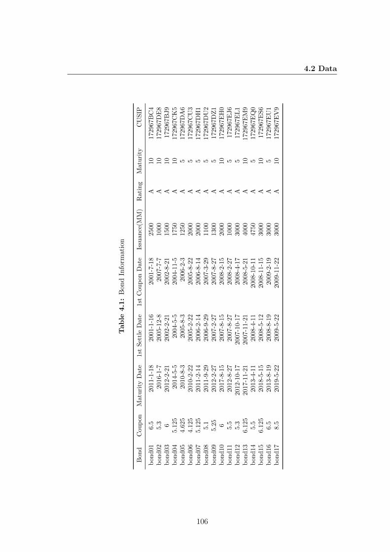
4.2 Data
Table
4.1:
Bon
dIn
form
atio
n
Bon
dC
oup
onM
atu
rity
Dat
e1s
tS
ettl
eD
ate
1st
Cou
pon
Date
Issu
an
ce(M
M)
Rati
ng
Matu
rity
CU
SIP
bon
d01
6.5
2011
-1-1
820
01-1
-16
2001-7
-18
2500
A10
172967B
C4
bon
d02
5.3
2016
-1-7
2005-1
2-8
2007-7
-71000
A10
172967D
E8
bon
d03
620
12-2
-21
2002-2
-21
2002-8
-21
1500
A10
172967B
J9
bon
d04
5.12
520
14-5
-52004-5
-52004-1
1-5
1750
A10
172967C
K5
bon
d05
4.62
520
10-8
-32005-8
-32006-2
-31250
A5
172967D
A6
bon
d06
4.12
520
10-2
-22
2005-2
-22
2005-8
-22
2000
A5
172967C
U3
bon
d07
5.12
520
11-2
-14
2006-2
-14
2006-8
-14
2000
A5
172967D
H1
bon
d08
5.1
2011
-9-2
920
06-9
-29
2007-3
-29
1100
A5
172967D
U2
bon
d09
5.25
2012
-2-2
720
07-2
-27
2007-8
-27
1300
A5
172967D
Z1
bon
d10
620
17-8
-15
2007-8
-15
2008-2
-15
2000
A10
172967E
H0
bon
d11
5.5
2012
-8-2
720
07-8
-27
2008-2
-27
1000
A5
172967E
J6
bon
d12
5.3
2012
-10-
1720
07-1
0-1
72008-4
-17
3000
A5
172967E
L1
bon
d13
6.12
520
17-1
1-21
2007-1
1-2
12008-5
-21
4000
A10
172967E
M9
bon
d14
5.5
2013
-4-1
120
08-4
-11
2008-1
0-1
14750
A5
172967E
Q0
bon
d15
6.12
520
18-5
-15
2008-5
-12
2008-1
1-1
53000
A10
172967E
S6
bon
d16
6.5
2013
-8-1
920
08-8
-19
2009-2
-19
3000
A5
172967E
U1
bon
d17
8.5
2019
-5-2
220
09-5
-22
2009-1
1-2
23000
A10
172967E
V9
106
4.2 Data
dealers. Because CMA receives prices from the buy-side community, who are
constantly receiving quotes from their dealers, these prices are very likely to be
tradable or even executable prices.1 These CDS spreads are mid-market price
quotes for contracts covering from 6-month to 10-year maturities. This enables
us to bootstrap hazard rates at any maturity within the range to match the
maturities of all the bonds issued by the company. Considering both the CDS
and corporate bond data we have, our analysis is conducted at a daily frequency.2
Finally, we choose Treasury rates as the risk-free rate, as it is widely used
by empirical studies in finance. The entire term structure of Treasury rates is
available from Federal Reserve H.15 Release3.
There are a few essential differences between market characterizations of cor-
porate bonds and CDSs, which are important for our applications.
Firstly, and most importantly, credit default swaps are contracts, not securi-
ties. Securities are in fixed supply, whereas the notional amount of credit default
swaps can be arbitrarily large. It may take time and effort to find a particular
corporate bond, whereas new credit default swaps of a underlying entity can be
created whenever they are needed. Moreover, the availability of CDS contracts
is not necessarily linked to the aggregate amount of reference bonds outstanding,
nor their maturities. In other words, CDS contracts are much less susceptible to
the market friction than the underlying corporate bonds.
Secondly, it is important to notice that credit default swaps are essentially
insurance contracts. Many investors who buy default protection may intend to
hold the position for a fixed time period, and may not generally plan to unwind
their position early. Even if an investor wants to unwind his current position,
it may be less costly to simply enter into a new swap in the opposite direction
1Mayordomo & Rodriguez-Moreno (2011) argue that the nature of the CMA data supposean advantage for the use of the bid-ask spread as a measure of liquidity because of the use ofinformation from the buy-sell sides.
2Bao et al. (2011) suggest that at daily frequency illiquidity effect is stronger.3Yields are interpolated by the Treasury from the daily yield curve. This curve, which
relates the yield on a security to its time to maturity is based on the closing market bid yieldson actively traded Treasury securities in the over-the-counter market. These market yields arecalculated from composites of quotations obtained by the Federal Reserve Bank of New York.The yield values are read from the yield curve at fixed maturities, currently 1, 3 and 6 monthsand 1, 2, 3, 5, 7, 10, 20, and 30 years.
107

4.2 Data
than to try to short his current position. Therefore, the liquidity of his current
position is less relevant since he is able to effectively replicate the short position
through other contracts.
Thirdly, a CDS investor buying or selling protection, only needs a fraction of
the principal (initial collateral margins or upfront fees), and the mark-to-market
effect of interest rate fluctuations to a position is usually negligible. It is generally
as easy to sell default protection as it is to buy default protection in CDS markets.
In contrast, sometimes it can be difficult and costly to short sell corporate bonds
due to limited arbitrage in the corporate bond market.
Finally, with the introduction of the new standard CDS contract and conven-
tions, and because of the generic nature of the cash flows, credit default swaps
cannot be demanded particularly in the way as Treasury securities or popular
equities may.
In the previous literature, empirical evidence is mixed. Ericsson et al. (2005)
use a set of credit risk models to evaluate the price of credit default swaps as
well as corporate bonds. They find that their models tend to systematically
underestimate bond spreads and, more importantly, that this is not the case for
CDS premia. They also find that bond spread residuals are largely unrelated
to default proxies but correlated with non-default proxies (such as illiquidity
proxies) and CDS premium residuals are uncorrelated with both. In other words,
the evidence supports the presence of illiquidity in bond residuals but not in
CDS residuals. Blanco et al. (2005) also provide evidence that changes in the
credit quality of the underlying name are likely to be reflected more quickly in
the default swap spreads than in the bond yield spreads. This may be due to
a non-default component in bond spreads that obscure the impact of changes in
credit quality. Ericsson et al. (2009) investigate the linear relationship between
theoretical determinants of default risk and default swap spreads. The principle
component analysis shows that there is limited evidence for a common factor in
the regression residuals. That implies that a liquidity-related component in credit
default swap spread may be negligible.
By contrast, Bongaerts et al. (2008) study the effect of liquidity on prices of
CDS from 2000 to 2006. They provide evidence of an economically and statisti-
cally significant expected liquidity premium attributable to the protection seller.
108

4.2 Data
Using data from 2002 to 2005, Lin et al. (2009) find both CDS and corporate
bond spreads contain significant liquidity components. Since there is no consen-
sus in the literature on whether CDS spreads contain a liquidity premium and
it is hard for us to check if CDS spreads contain a liquidity premium as that
requires a long history of default data, this study follows Longstaff et al. (2005)
in assuming that CDS spreads do not contain a liquidity premium.
109
4.3 The Methodology
4.3 The Methodology
In this section, first, we discuss the valuation of bonds and credit default swaps
in our non-parametric framework. Second, we elaborate on the assumption of
a constant recovery rate as well as the tenor effects in term structures post the
crisis. Third, descriptive statistics of the estimated non-default price residuals are
provided. Fourth, a detailed instruction of computing non-default price residuals
of a corporate bond is given. Fifthly, we introduce the extended Roll model to
estimate our liquidity measure as well as the non-default yield spread. Finally,
summary statistics of the non-default yield spread and the liquidity measure are
reported.
4.3.1 Valuing Bonds and Credit Default Swaps
Following Longstaff et al. (2005), we treat CDSs as a benchmark, that is, we
explain credit default swap spreads by only default risk (in terms of default prob-
ability) and apply the default probabilities backed out from the credit default
swap spreads of the same underlying entity to obtain the ‘fundamental value’ of
a corresponding corporate bond.1
We value credit default swaps and corporate bonds within the reduced-form
framework of Duffie & Singleton (1999). But, different from Longstaff et al.
(2005), we apply a non-parametric valuation approach in order to generate more
flexible shapes of default intensity term structures.
Let D(t, T ) denote the riskless discount factors at time t for maturity T and
assume them to be independent of the default time τ . The probability of the
name survives up to time T , observed at time 0, can be expressed as
Surv(T ) := Prob(τ > T ) (4.1)
The conditions for a valid survival probability function are Surv(0) = 1, Surv(t) >
0 and Surv(·) needs to be decreasing. By following the market, Surv(t) is defined
1The ‘fundamental value’ equals the value of a hypothetical liquid defaultable bond withthe same maturity date and coupon rate.
110

4.3 The Methodology
as
exp(−H(t)) = exp(−∫ t
0
h(s)ds), (4.2)
where the hazard rate h is assumed to be piecewise constant1 in time, eg. h(t) = hi
for t in [Ti−1, Ti]. Let 4i denote the accrual period from Ti−1 to Ti. The value of
the premium of a CDS at time 0 can be decomposed into the value of an annuity
paying one basis point and its accrual fee paid upon default, scaled by the spot
running spread:
PremLegN(SN ;D(0, ·), Surv(·))
= SN · (AnnuN(D(0, ·), Surv(·)) + AccrN(D(0, ·), Surv(·))),(4.3)
where
AnnuN(D(0, ·), Surv(·)) =N∑i=1
D(0, Ti)4i exp(−H(Ti)) (4.4)
and
AccrN(D(0, ·), Surv(·)) =N∑i=1
D(0, Ti)4i
2(exp(−H(Ti−1))− exp(−H(Ti))).
(4.5)
Note 4i2
is the average accrual period from Ti−1 to Ti and exp(−H(Ti−1)) −exp(−H(Ti)) is the probability of a credit event occurring during period Ti−1 to
Ti.
By assuming recovery of the face value in the event of default, the valuation
of the protection leg can be expressed similarly as
ProtLegN(R;D(0, ·), Surv(·))
= −(1−R)
∫ TN
0
D(0, s)dSurv(s)
≈ (1−R)M∑j=1
D(0, tj)(exp(−H(tj−1))− exp(−H(tj))),
(4.6)
1We also tried piecewise linear hazard rate term structure. The results generally remainthe same as we have data of CDS spreads at all maturities (1,2,3, up to 10 years).
111
4.3 The Methodology
where the Stieltjes integral is replaced by Riemann sums taken on a low enough
discretization time steps tj, j = 1, ...,M , given t0 = 0 and tM = TN .
Equating the values of the two legs and solving for the running spread gives
SN =(1−R)
∑Mj=1 D(0, tj)(exp(−H(tj−1))− exp(−H(tj)))∑N
i=1 D(0, Ti)4i[exp(−H(Ti)) + 12(exp(−H(Ti−1))− exp(−H(Ti)))]
.
(4.7)
Under the same framework, the ’fair value’ of a defaultable bond with coupon
c, face value F and maturity N can be expressed as
CPN = c ·N∑i=1
D(0, Ti)4i exp(−H(Ti))
+ F ·D(0, TN) exp(−H(TN))
+RM∑j=1
D(0, tj)(exp(−H(tj−1))− exp(−H(tj))),
(4.8)
where R is the recovery rate which is kept consistent to the recovery assumption
in the CDS pricing formulas with corresponding seniority and maturity.
4.3.2 Recovery Rate Assumption
The assumption of a constant recovery rate is often adopted for modelling and
estimation purposes in many credit literature. However, very few of them check
whether the assumption of recovery rates has any impact on the valuation. Re-
covery rates generally can be treated in two ways. The first method is to consider
it as another parameter, and to estimate it from the data along with other pa-
rameters. The second one is to a priori fix a value.
Now let us have a look at the relationship between recovery rates and default
probabilities in a simply case: the valuation of a risky zero-coupon bond in one-
period. Assuming the riskless rate is zero, consider the price of a defaultable
zero-coupon bondZCP = Prob ·R + (1− Prob)
= 1− Prob · (1−R)(4.9)
112
4.3 The Methodology
Then the valuation equation for CDS spreads is given by
S · (1− Prob) = (1−R) · Prob. (4.10)
We find that the credit spread or CDS spread S is given by
S = −(1−R)(1− 1
1− Prob)
≈ (1−R) · Prob.(4.11)
Note that both bond prices and CDS spreads are actually expressed by the prod-
uct of the expected loss (1 − R) and the default probability Prob. It turns out
that it is hard to identify both the recovery rate and the default probability from
only one data source, either bond prices or CDS spreads. This may pose a prob-
lem for some applications. For example, if market participants think the recovery
rate was 50%, but 40% was put in the formulas for calculating the upfront fee
for CDSs, then the hazard rate or the default probability must move down to
balance the larger loss incurred in the event of default. The difference between
the expected recovery rate and the assumed constant recovery rate will result in
a cheaper upfront fee, and therefore affect the conversion.
Fortunately, for our purpose of obtaining the fundamental value of a corporate
bond using CDS spreads, this does not cause any problem. Figure 4.1 shows the
price of a generic bond with 5-year maturity for varying recovery rates (and thus
varying default probabilities). The bond price increases very slowly when the
recovery rate is below 70%. As long as the recovery rate is kept between 10%
and 70%, the differences between estimated bond yields are essentially within 10
bps. Therefore, the defaultable bond price is relatively insensitive to the assumed
recovery rate. Therefore, following the market convention, the recovery rate for
senior unsecured corporate bonds is assumed to be 40%, as well as for senior CDS
contracts.
113

4.3 The Methodology
Figure 4.1: Sensitivity of Bond Prices to the Recovery Rate
A reduced form model with piecewise constant hazard rate term structure isused to price corporate bonds under the assumption of constant recovery rate.
114
4.3 The Methodology
4.3.3 Tenor Effects in the Term Structure
Since the beginning of the financial crisis in August 2007, the money markets
have exhibited an unprecedented behaviour. Interest rates, like for instance swap
rates with the same tenor but based on different floating-leg frequencies, that
previously had been following each other closely for a long time, have started to
keep a significant distance apart. This divergence in values does not create arbi-
trage opportunities when credit or liquidity issues are taken into account, which
means that the market is not pricing with a unique term structure any more.
The assumption of a unique discounting curve has been forsaken by practition-
ers, who seem to agree on an empirical approach based on the construction of
as many curves as possible rate tenors. For each given contract, they select a
specific discount curve, which they use to calculate the net present value (NPV)
of the contract’s future payments, consistently with the contract’s features such
as tenors or counterparties in question.1
All corporate bonds in our sample pay semi-annual coupons. Therefore, tenor
effects will not be a concern for our applications, as long as we keep the same
practice of building discounting curves for all bonds. To construct a riskless
discount curve, we download the Constant Maturity Treasury rates of maturities
0.5-year, 1-year, 2-year, 3-year, 5-year, 7-year and 10-year from Federal Reserve
website. We first interpolate these par rates at semiannual intervals by using
cubic spline. Then spot rates are obtained by bootstrapping these par rates at
semiannual intervals. A whole discount curve is provided by linearly interpolating
the corresponding forward curve.
1The valuation of interest rate derivatives under different curves, for generating future ratesand for discounting has received a lot of attention in the financial literature recently. Previousworks that started to deal with these issues, mainly concerning the valuation of cross currencyswaps, are Boenkost & Schmidt (2005), Kijima et al. (2008) and Henrard (2007). Bianchetti(2010), was the first to apply the methodology to the single currency case, while Chibane &Sheldon (2009) propose methods to extend yield curve bootstrapping to a multi-curve setting.In terms of new pricing models, Kijima et al. (2008), Mercurio (2010a) and Mercurio (2010b)apply the method using a stochastic volatility LMM, in order to price calets and swaptions,while Moreni & Pallavicini (2010), apply the new framework under the HJM model.
115

4.3 The Methodology
4.3.4 Computing Non-default Price Residuals of a Corpo-
rate Bond
To compute the non-default price residuals of a corporate bond, we use the fol-
lowing procedure. Firstly, a riskless discount function D(0, ·) is needed for each
trading date. The constant maturity 6-month, 1-year, up to 10-year Treasury
rates are downloaded from the Federal Reserve website. Then these par rates are
interpolated at semiannual intervals by using a cubic spline algorithm. A discount
curve at semiannual intervals can be obtained by bootstrapping the interpolated
par rates. A linear interpolation of the corresponding forward rates is applied to
provide the value of D(0, ·) at other maturities.
Secondly, given the discount curve and the mid-quotes of the CDS contracts
covering from 6-month to 10-year maturities, on each trading day a term structure
of hazard rates can be bootstrapped by using Equation 4.7 under the assumption
of a piecewise constant hazard rate term structure. Then, a survival probability
function Surv(·) is obtained by using Equation 4.2.
Thirdly, given the discount curve D(0, ·) and the survival probability func-
tion Surv(·), a ‘fundamental price’ of the corresponding corporate bond can be
computed by using Equation 4.8. In other words, the ‘fundamental price’ of a
corporate bond is equal to the value of a hypothetical liquid defaultable bond
with the same maturity date and coupon rate.
Finally, subtracting the market-based transaction prices from the model-based
‘fundamental prices’ gives the non-default price residuals of a corporate bond.
This procedure is similar to the one implemented in Longstaff et al. (2005). How-
ever, our approach does not depend on a parametric credit risk model, and is able
to generate very flexible shapes of hazard rate term structures. It is important
to notice that there is no regression involved in the procedure of computing the
non-default price residuals.
116
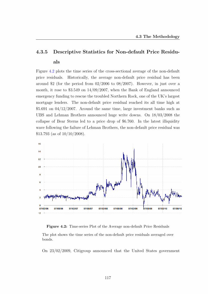
4.3 The Methodology
4.3.5 Descriptive Statistics for Non-default Price Residu-
als
Figure 4.2 plots the time series of the cross-sectional average of the non-default
price residuals. Historically, the average non-default price residual has been
around $2 (for the period from 02/2006 to 08/2007). However, in just over a
month, it rose to $3.549 on 14/09/2007, when the Bank of England announced
emergency funding to rescue the troubled Northern Rock, one of the UK’s largest
mortgage lenders. The non-default price residual reached its all time high at
$5.691 on 04/12/2007. Around the same time, large investment banks such as
UBS and Lehman Brothers announced huge write downs. On 18/03/2008 the
collapse of Bear Sterns led to a price drop of $6.760. In the latest illiquidity
wave following the failure of Lehman Brothers, the non-default price residual was
$13.793 (as of 10/10/2008).
Figure 4.2: Time-series Plot of the Average non-default Price Residuals
The plot shows the time series of the non-default price residuals averaged overbonds.
On 23/02/2009, Citigroup announced that the United States government
117
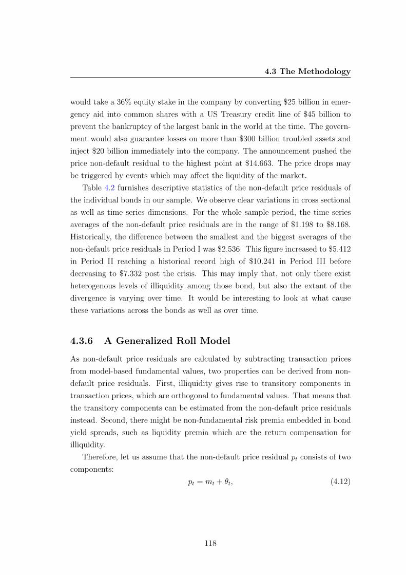
4.3 The Methodology
would take a 36% equity stake in the company by converting $25 billion in emer-
gency aid into common shares with a US Treasury credit line of $45 billion to
prevent the bankruptcy of the largest bank in the world at the time. The govern-
ment would also guarantee losses on more than $300 billion troubled assets and
inject $20 billion immediately into the company. The announcement pushed the
price non-default residual to the highest point at $14.663. The price drops may
be triggered by events which may affect the liquidity of the market.
Table 4.2 furnishes descriptive statistics of the non-default price residuals of
the individual bonds in our sample. We observe clear variations in cross sectional
as well as time series dimensions. For the whole sample period, the time series
averages of the non-default price residuals are in the range of $1.198 to $8.168.
Historically, the difference between the smallest and the biggest averages of the
non-default price residuals in Period I was $2.536. This figure increased to $5.412
in Period II reaching a historical record high of $10.241 in Period III before
decreasing to $7.332 post the crisis. This may imply that, not only there exist
heterogenous levels of illiquidity among those bond, but also the extant of the
divergence is varying over time. It would be interesting to look at what cause
these variations across the bonds as well as over time.
4.3.6 A Generalized Roll Model
As non-default price residuals are calculated by subtracting transaction prices
from model-based fundamental values, two properties can be derived from non-
default price residuals. First, illiquidity gives rise to transitory components in
transaction prices, which are orthogonal to fundamental values. That means that
the transitory components can be estimated from the non-default price residuals
instead. Second, there might be non-fundamental risk premia embedded in bond
yield spreads, such as liquidity premia which are the return compensation for
illiquidity.
Therefore, let us assume that the non-default price residual pt consists of two
components:
pt = mt + θt, (4.12)
118
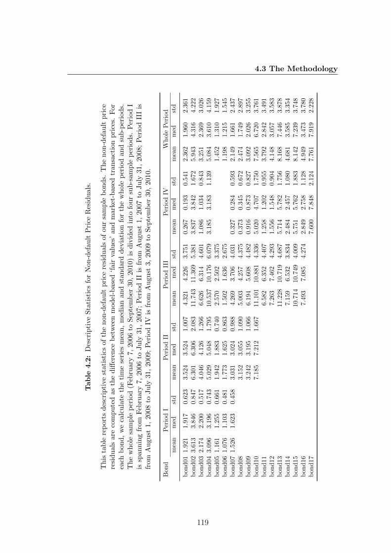
4.3 The Methodology
Table
4.2:
Des
crip
tive
Sta
tist
ics
for
Non
-def
ault
Pri
ceR
esid
ual
s.
Th
ista
ble
rep
orts
des
crip
tive
stati
stic
sof
the
non
-def
ault
pri
cere
sid
ual
sof
our
sam
ple
bon
ds.
Th
en
on-d
efau
ltp
rice
resi
du
als
are
com
pu
ted
as
the
diff
eren
ceb
etw
een
mod
el-b
ased
‘fai
rva
lues
’an
dm
arke
t-b
ased
tran
sact
ion
pri
ces.
For
each
bond
,w
eca
lcu
late
the
tim
ese
ries
mea
n,
med
ian
and
stan
dar
ddev
iati
onfo
rth
ew
hol
ep
erio
dan
dsu
b-p
erio
ds.
Th
ew
hole
sam
ple
per
iod
(Feb
ruary
7,
2006
toS
epte
mb
er30
,20
10)
isd
ivid
edin
tofo
ur
sub
-sam
ple
per
iod
s.P
erio
dI
issp
ann
ing
from
Feb
ruary
7,2006
toJu
ly31
,20
07;
Per
iod
IIis
from
Au
gust
1,20
07to
Ju
ly31
,20
08;
Per
iod
III
isfr
om
Au
gust
1,
2008
toJuly
31,
2009;
Per
iod
IVis
from
Au
gust
3,20
09to
Sep
tem
ber
30,
2010
.
Bon
dP
erio
dI
Per
iod
IIP
erio
dII
IP
erio
dIV
Wh
ole
Per
iod
mea
nm
edst
dm
ean
med
std
mea
nm
edst
dm
ean
med
std
mea
nm
edst
d
bon
d01
1.92
11.
917
0.62
33.
524
3.52
41.0
07
4.3
21
4.2
26
3.7
51
0.2
67
0.1
93
0.5
41
2.3
62
1.9
60
2.3
61
bon
d02
3.61
33.
846
0.84
76.
301
6.30
62.0
83
11.7
43
11.3
69
5.3
81
3.8
37
3.8
42
1.6
72
5.9
43
4.3
16
4.2
22
bon
d03
2.17
42.
200
0.51
74.
046
4.12
61.2
66
6.6
26
6.3
14
4.6
01
1.0
86
1.0
34
0.8
43
3.2
51
2.3
69
3.0
26
bon
d04
3.09
63.
196
0.74
35.
029
5.04
81.7
95
10.5
37
10.1
76
6.0
79
3.1
85
3.1
83
1.1
39
5.0
84
3.6
10
4.1
59
bon
d05
1.16
11.
255
0.66
11.
942
1.88
30.7
40
2.5
70
2.5
02
3.3
75
1.4
52
1.3
10
1.9
27
bon
d06
1.07
61.
103
0.48
11.
773
1.62
50.8
63
1.5
02
1.6
36
2.6
75
1.1
98
1.2
15
1.5
45
bon
d07
1.52
61.
623
0.45
83.
031
3.02
40.9
88
4.2
69
3.7
06
4.0
31
0.3
27
0.2
84
0.5
93
2.1
49
1.6
61
2.4
37
bon
d08
3.15
23.
055
1.0
90
5.0
03
4.2
57
4.3
75
0.3
73
0.3
45
0.6
72
2.4
74
1.7
49
2.8
97
bon
d09
3.24
23.
195
1.0
66
6.1
94
5.6
08
4.4
82
0.9
16
0.8
73
0.8
27
3.0
92
2.0
26
3.2
55
bon
d10
7.18
57.
212
1.6
67
11.1
01
10.8
81
4.3
36
5.0
20
4.7
07
1.7
50
7.5
65
6.7
20
3.7
61
bon
d11
6.5
82
6.3
52
4.4
07
1.2
58
1.2
02
0.9
55
3.7
92
2.8
42
3.4
91
bon
d12
7.2
63
7.4
62
4.2
93
1.5
56
1.5
48
0.9
04
4.1
48
3.0
57
3.5
83
bon
d13
11.2
28
10.7
19
4.6
87
5.7
14
5.7
82
1.7
56
8.1
68
7.4
46
3.8
78
bon
d14
7.1
59
6.5
32
3.8
34
2.4
84
2.4
57
1.0
80
4.6
81
3.5
85
3.3
54
bon
d15
10.7
14
10.7
49
4.0
09
5.7
51
5.7
62
1.8
83
8.1
42
7.2
39
3.7
48
bon
d16
7.4
93
7.0
85
4.2
74
2.8
49
2.7
58
1.1
28
4.9
49
3.4
73
3.7
80
bon
d17
7.6
00
7.8
48
2.1
24
7.7
61
7.9
19
2.2
28
119
4.3 The Methodology
The first component mt represents the permanent price effect, reflecting the unan-
ticipated information received by market participants, including the information
about the future illiquidity of the bonds. The permanent component is assumed
to follow a random walk process:
mt = mt−1 + εt, (4.13)
where εt describes changes in prices due to new information.
The second component θt comes from costs of illiquidity, which is transitory
and uncorrelated with the fundamental value. The absolute value of the transitory
component θt is essentially our illiquidity measure, which characterizes the degree
of current illiquidity in the market.
Now, let us assume that the transitory component θt is equal to a serially
uncorrelated disturbance, νt, with mean zero and variance Ht, and the innovation
term of the permanent component εt has mean zero and variance Qt. However,
in our application both νt and εt are i.i.d. normally distributed, and both H and
Q are independent of time.
The estimation of the state space model is carried out via a Kalman filter
approach by numerically maximizing the relevant log-likelihood function. Fur-
thermore, we assume νt ∼ N(0, H) with H = exp(c1) and εt ∼ N(0, Q) with
Q = exp(c2). The underlying volatility is computed as√Q. The model is esti-
mated respectively for each bond and each sub-period.
The estimates of the model parameters c1 and c2 are reported in Table 4.3.
The results show that the cross-sectional average of the underlying volatility was
0.047 prior to the crisis.1 It jumped to 0.266 in Period II and then reached the
highest level at 0.768 in Period III, before coming back to 0.247 post the crisis
period. The obvious structural breaks in the data force us to estimate the model
period by period.
We can also observe some degree of contemporaneous heteroscedasticity across
different bonds. Figure 4.3 plots the underlying volatilities of the 5-year and
10-year bonds, respectively, against their corresponding maturity dates in four
1It is important to notice that these volatilities are those of the unobservable non-defaultprice discounts, as the analysis is focusing on non-default bond residuals.
120
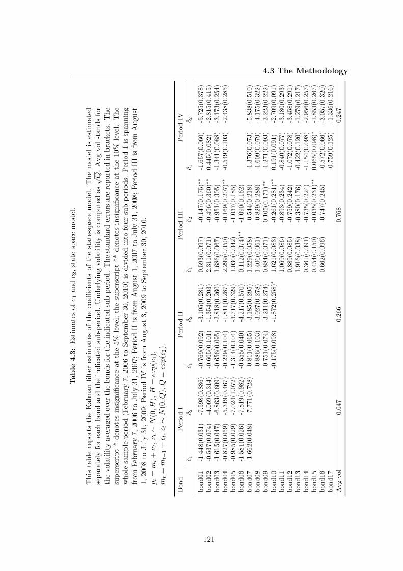
4.3 The MethodologyTable
4.3:
Est
imat
esofc 1
andc 2
,st
ate
spac
em
od
el.
Th
ista
ble
rep
ort
sth
eK
alm
anfi
lter
esti
mat
esof
the
coeffi
cien
tsof
the
stat
e-sp
ace
mod
el.
Th
em
od
elis
esti
mat
edse
par
atel
yfo
rea
chb
ond
an
dth
ein
dic
ate
dsu
b-p
erio
d.
Un
der
lyin
gvo
lati
lity
isco
mp
ute
das√Q
.A
vg
vol
stan
ds
for
the
vola
tili
tyav
erag
edov
erth
eb
on
ds
for
the
ind
icat
edsu
b-p
erio
d.
Th
est
and
ard
erro
rsar
ere
por
ted
inb
rack
ets.
Th
esu
per
scri
pt
*d
enot
esin
sign
ifica
nce
at
the
5%le
vel;
the
sup
ersc
rip
t**
den
otes
insi
gnifi
can
ceat
the
10%
leve
l.T
he
wh
ole
sam
ple
per
iod
(Feb
ruar
y7,
2006
toS
epte
mb
er30
,20
10)
isd
ivid
edin
tofo
ur
sub-p
erio
ds.
Per
iod
Iis
span
nin
gfr
omF
ebru
ary
7,20
06
toJu
ly31
,2007
;P
erio
dII
isfr
omA
ugu
st1,
2007
toJu
ly31
,20
08;
Per
iod
III
isfr
omA
ugu
st1,
200
8to
Ju
ly31
,2009
;P
erio
dIV
isfr
omA
ugu
st3,
2009
toS
epte
mb
er30
,20
10.
pt
=mt+ν t
,ν t∼N
(0,H
),H
=exp(c
1),
mt
=mt−
1+ε t
,ε t∼N
(0,Q
),Q
=exp(c
2).
Bon
dP
erio
dI
Per
iod
IIP
erio
dII
IP
erio
dIV
c 1c 2
c 1c 2
c 1c 2
c 1c 2
bon
d01
-1.4
48(0
.031
)-7
.598
(0.8
86)
-0.7
69(0
.092)
-3.1
05(0
.281)
0.5
93(0
.097)
-0.1
47(0
.175)∗
∗-1
.657(0
.060)
-5.7
25(0
.378)
bon
d02
-0.5
37(0
.074
)-4
.069
(0.3
14)
-0.6
05(0
.101)
-1.3
54(0
.203)
2.3
11(0
.071)
-0.4
96(0
.360)∗
∗0.4
45(0
.082)
-2.8
15(0
.415)
bon
d03
-1.6
15(0
.047
)-6
.863
(0.6
09)
-0.6
56(0
.095)
-2.8
18(0
.260)
1.6
86(0
.067)
-0.9
51(0
.305)
-1.3
41(0
.088)
-3.1
73(0
.254)
bon
d04
-0.8
27(0
.059
)-5
.319
(0.4
67)
-0.2
29(0
.104)
-1.8
11(0
.287)
2.2
99(0
.050)
-0.1
69(0
.207)∗
∗-0
.549(0
.103)
-2.4
38(0
.285)
bon
d05
-0.9
85(0
.029
)-7
.024
(1.0
72)
-1.3
14(0
.104)
-3.7
17(0
.329)
1.0
30(0
.042)
-1.0
37(0
.185)
bon
d06
-1.5
81(0
.026
)-7
.819
(0.9
82)
-0.5
55(0
.040)
-4.2
17(0
.570)
0.1
12(0
.074)∗
∗-1
.090(0
.162)
bon
d07
-1.6
62(0
.048
)-7
.771
(0.7
28)
-0.8
11(0
.065)
-3.1
85(0
.295)
1.2
29(0
.058)
-0.5
44(0
.218)
-1.3
76(0
.073)
-5.8
38(0
.510)
bon
d08
-0.8
86(0
.103)
-3.0
27(0
.278)
1.4
06(0
.061)
-0.8
29(0
.288)
-1.6
09(0
.079)
-4.1
75(0
.322)
bon
d09
-0.7
51(0
.074)
-3.2
11(0
.274)
0.8
84(0
.071)
0.1
05(0
.171)∗
∗-1
.271(0
.093)
-3.2
23(0
.222)
bon
d10
-0.1
75(0
.098)
-1.8
72(0
.258)∗
1.6
21(0
.083)
-0.2
61(0
.281)∗
∗0.1
91(0
.091)
-2.7
09(0
.091)
bon
d11
1.0
69(0
.086)
-0.8
93(0
.234)
-0.8
40(0
.077)
-3.1
80(0
.293)
bon
d12
0.8
89(0
.085)
-0.7
59(0
.242)
-1.0
72(0
.078)
-3.4
58(0
.291)
bon
d13
1.9
16(0
.038)
-0.3
80(0
.176)
-0.4
22(0
.120)
-1.2
79(0
.217)
bon
d14
0.3
61(0
.091)
-0.7
35(0
.224)
-1.1
54(0
.098)
-2.9
56(0
.257)
bon
d15
0.4
54(0
.150)
-0.0
35(0
.231)∗
∗0.0
65(0
.098)∗
-1.8
53(0
.267)
bon
d16
0.6
62(0
.096)
-0.7
47(0
.245)
-0.5
72(0
.066)
-3.0
57(0
.320)
bon
d17
-0.7
59(0
.125)
-1.3
36(0
.216)
Avg
vol
0.04
70.2
66
0.7
68
0.2
47
121
4.3 The Methodology
sub-periods, separately. As we can see, the volatility curves are generally linear
and positively sloped, indicating that uncertainty about future liquidity increases
in the time-to-maturity. In Period III and IV, there are a few outliers, which are
the bonds with small or medium issue sizes, indicating that issue sizes might be
the possible omitted variable.
In addition, we check whether the estimated unobservable non-default price
residuals mt are integrated of order one as the model assumes. In order to de-
termine the order of integration of mt for each bond in each sub-period, we use
Augmented Dickey-Fuller (ADF) tests with Mackinnon’s critical values. Table
4.4 reports the results (t-statistics) of the tests of the null hypothesis of a unit
root in mt. If the t-statistics differ significantly from zero, the null hypothesis of
existence of a unit root is reject and stationarity is concluded. We test for unit
roots in mt of each bond in each sub-period in terms of levels and first differences.
The ADF tests indicate that for almost all the series of mt the null hypothesis of
existence of a unit root cannot be rejected.
4.3.7 Preliminary Analysis on Unobservable Non-default
Yield Spread and Illiquidity Measure
Now, it is time to turn to the elements which we are really interested in, namely,
the unobservable non-default price discount mt (or in terms of yield) and the
illiquidity measure st. Table 4.5 reports the means and the standard deviations
of the estimated unobservable non-default price discounts mt for each bond in
the indicated sub-periods. The cross-sectional averages of the means of mt rose
from a level of about $2 in Period I to about $4 in Period II. In Period III, the
cross-sectional average increased dramatically to more than $7. Similar to the
volatility, post the crisis the unobservable non-default price discounts came back
to about the same level prior to the crisis. The results suggest that there exist
common processes that are driving the non-default components across the bonds.
Cross-sectionally, the time series averages of mt in Period I ranged from $3.605 to
$1.077, whereas in Period II, III, and IV they ranged from $7.018 to $1.761, from
$11.7657 to $1.505, and $7.605 to $0.276. In particular, the difference between
122

4.3 The Methodology
01/01/10 08/05/12 13/09/14 18/01/17 26/05/190
0.2
0.4
0.6
0.8
1
1.2
Maturity
Und
erly
ing
Vol
atili
ty
Period I
10−year5−year
01/01/10 08/05/12 13/09/14 18/01/17 26/05/190
0.2
0.4
0.6
0.8
1
1.2
Maturity
Und
erly
ing
Vol
atili
ty
Period II
10−year5−year
01/01/10 08/05/12 13/09/14 18/01/17 26/05/190
0.2
0.4
0.6
0.8
1
1.2
Maturity
Und
erly
ing
Vol
atili
ty
Period III
10−year5−year
01/01/10 08/05/12 13/09/14 18/01/17 26/05/190
0.2
0.4
0.6
0.8
1
1.2
Maturity
Und
erly
ing
Vol
atili
ty
Period IV
10−year5−year
Figure 4.3: Cross-sectional Plots of Underlying Volatility against MaturityDate
This figure plots the average underlying volatilities of the 5-year and 10-yearbonds against their maturity dates, respectively. > 10-year denotes 10-yearbond; 5-year denotes 5-year bond. Issue size might be the possible omittedvariable.
123
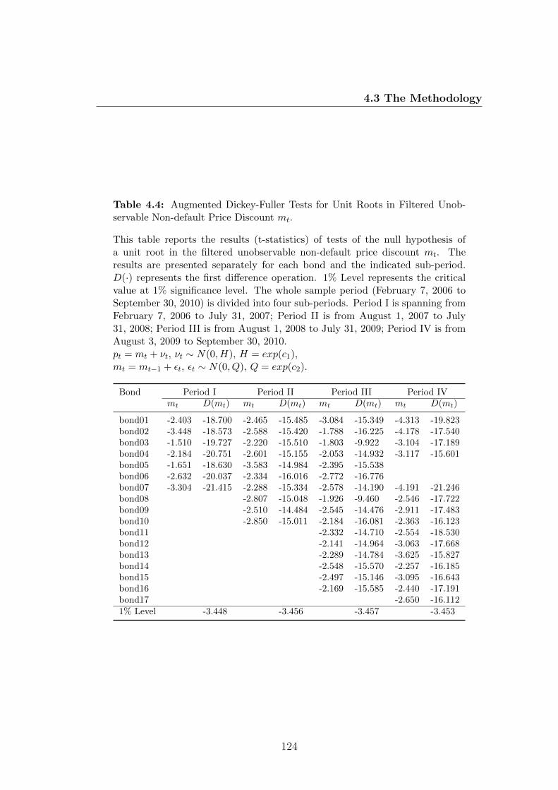
4.3 The Methodology
Table 4.4: Augmented Dickey-Fuller Tests for Unit Roots in Filtered Unob-servable Non-default Price Discount mt.
This table reports the results (t-statistics) of tests of the null hypothesis ofa unit root in the filtered unobservable non-default price discount mt. Theresults are presented separately for each bond and the indicated sub-period.D(·) represents the first difference operation. 1% Level represents the criticalvalue at 1% significance level. The whole sample period (February 7, 2006 toSeptember 30, 2010) is divided into four sub-periods. Period I is spanning fromFebruary 7, 2006 to July 31, 2007; Period II is from August 1, 2007 to July31, 2008; Period III is from August 1, 2008 to July 31, 2009; Period IV is fromAugust 3, 2009 to September 30, 2010.pt = mt + νt, νt ∼ N(0, H), H = exp(c1),mt = mt−1 + εt, εt ∼ N(0, Q), Q = exp(c2).
Bond Period I Period II Period III Period IVmt D(mt) mt D(mt) mt D(mt) mt D(mt)
bond01 -2.403 -18.700 -2.465 -15.485 -3.084 -15.349 -4.313 -19.823bond02 -3.448 -18.573 -2.588 -15.420 -1.788 -16.225 -4.178 -17.540bond03 -1.510 -19.727 -2.220 -15.510 -1.803 -9.922 -3.104 -17.189bond04 -2.184 -20.751 -2.601 -15.155 -2.053 -14.932 -3.117 -15.601bond05 -1.651 -18.630 -3.583 -14.984 -2.395 -15.538bond06 -2.632 -20.037 -2.334 -16.016 -2.772 -16.776bond07 -3.304 -21.415 -2.288 -15.334 -2.578 -14.190 -4.191 -21.246bond08 -2.807 -15.048 -1.926 -9.460 -2.546 -17.722bond09 -2.510 -14.484 -2.545 -14.476 -2.911 -17.483bond10 -2.850 -15.011 -2.184 -16.081 -2.363 -16.123bond11 -2.332 -14.710 -2.554 -18.530bond12 -2.141 -14.964 -3.063 -17.668bond13 -2.289 -14.784 -3.625 -15.827bond14 -2.548 -15.570 -2.257 -16.185bond15 -2.497 -15.146 -3.095 -16.643bond16 -2.169 -15.585 -2.440 -17.191bond17 -2.650 -16.1121% Level -3.448 -3.456 -3.457 -3.453
124
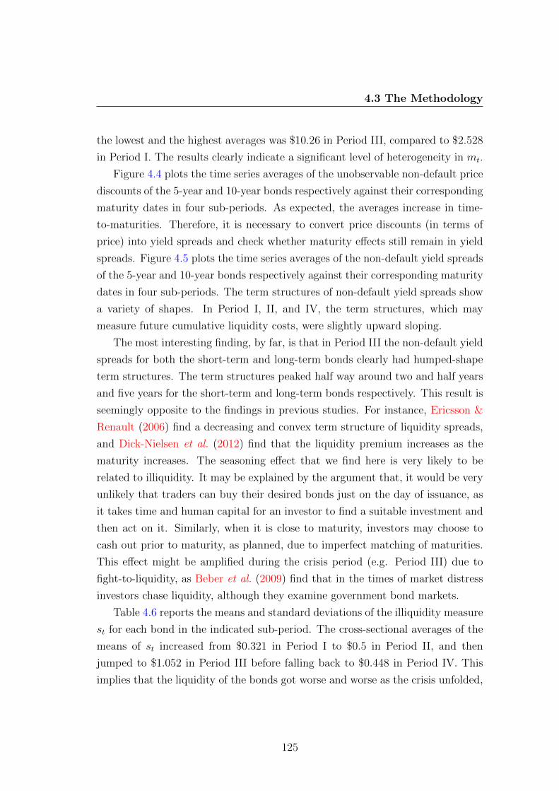
4.3 The Methodology
the lowest and the highest averages was $10.26 in Period III, compared to $2.528
in Period I. The results clearly indicate a significant level of heterogeneity in mt.
Figure 4.4 plots the time series averages of the unobservable non-default price
discounts of the 5-year and 10-year bonds respectively against their corresponding
maturity dates in four sub-periods. As expected, the averages increase in time-
to-maturities. Therefore, it is necessary to convert price discounts (in terms of
price) into yield spreads and check whether maturity effects still remain in yield
spreads. Figure 4.5 plots the time series averages of the non-default yield spreads
of the 5-year and 10-year bonds respectively against their corresponding maturity
dates in four sub-periods. The term structures of non-default yield spreads show
a variety of shapes. In Period I, II, and IV, the term structures, which may
measure future cumulative liquidity costs, were slightly upward sloping.
The most interesting finding, by far, is that in Period III the non-default yield
spreads for both the short-term and long-term bonds clearly had humped-shape
term structures. The term structures peaked half way around two and half years
and five years for the short-term and long-term bonds respectively. This result is
seemingly opposite to the findings in previous studies. For instance, Ericsson &
Renault (2006) find a decreasing and convex term structure of liquidity spreads,
and Dick-Nielsen et al. (2012) find that the liquidity premium increases as the
maturity increases. The seasoning effect that we find here is very likely to be
related to illiquidity. It may be explained by the argument that, it would be very
unlikely that traders can buy their desired bonds just on the day of issuance, as
it takes time and human capital for an investor to find a suitable investment and
then act on it. Similarly, when it is close to maturity, investors may choose to
cash out prior to maturity, as planned, due to imperfect matching of maturities.
This effect might be amplified during the crisis period (e.g. Period III) due to
fight-to-liquidity, as Beber et al. (2009) find that in the times of market distress
investors chase liquidity, although they examine government bond markets.
Table 4.6 reports the means and standard deviations of the illiquidity measure
st for each bond in the indicated sub-period. The cross-sectional averages of the
means of st increased from $0.321 in Period I to $0.5 in Period II, and then
jumped to $1.052 in Period III before falling back to $0.448 in Period IV. This
implies that the liquidity of the bonds got worse and worse as the crisis unfolded,
125
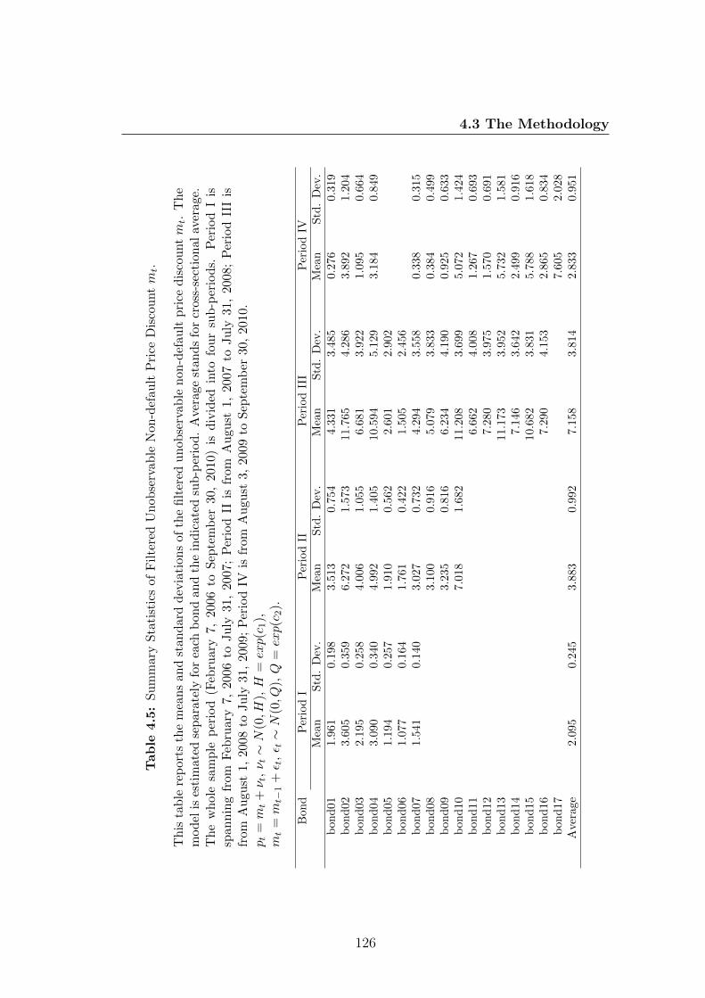
4.3 The Methodology
Table
4.5:
Su
mm
ary
Sta
tist
ics
ofF
ilte
red
Un
obse
rvab
leN
on-d
efau
ltP
rice
Dis
cou
ntmt.
Th
ista
ble
rep
orts
the
mea
ns
an
dst
and
ard
dev
iati
ons
ofth
efi
lter
edu
nob
serv
able
non
-def
ault
pri
ced
isco
untmt.
Th
em
od
elis
esti
mat
edse
par
ate
lyfo
rea
chb
ond
and
the
ind
icat
edsu
b-p
erio
d.
Ave
rage
stan
ds
for
cros
s-se
ctio
nal
aver
age.
Th
ew
hol
esa
mp
lep
erio
d(F
ebru
ary
7,20
06to
Sep
tem
ber
30,
2010
)is
div
ided
into
fou
rsu
b-p
erio
ds.
Per
iod
Iis
span
nin
gfr
omF
ebru
ary
7,
200
6to
Ju
ly31
,20
07;
Per
iod
IIis
from
Au
gust
1,20
07to
Ju
ly31
,20
08;
Per
iod
III
isfr
om
Au
gust
1,
2008
toJuly
31,
2009;
Per
iod
IVis
from
Au
gust
3,20
09to
Sep
tem
ber
30,
2010
.pt
=mt+ν t
,ν t∼N
(0,H
),H
=exp(c
1),
mt
=mt−
1+ε t
,ε t∼N
(0,Q
),Q
=exp(c
2).
Bon
dP
erio
dI
Per
iod
IIP
erio
dII
IP
erio
dIV
Mea
nS
td.
Dev
.M
ean
Std
.D
ev.
Mea
nS
td.
Dev
.M
ean
Std
.D
ev.
bon
d01
1.96
10.
198
3.5
13
0.7
54
4.3
31
3.4
85
0.2
76
0.3
19
bon
d02
3.60
50.
359
6.2
72
1.5
73
11.7
65
4.2
86
3.8
92
1.2
04
bon
d03
2.19
50.
258
4.0
06
1.0
55
6.6
81
3.9
22
1.0
95
0.6
64
bon
d04
3.09
00.
340
4.9
92
1.4
05
10.5
94
5.1
29
3.1
84
0.8
49
bon
d05
1.19
40.
257
1.9
10
0.5
62
2.6
01
2.9
02
bon
d06
1.07
70.
164
1.7
61
0.4
22
1.5
05
2.4
56
bon
d07
1.54
10.
140
3.0
27
0.7
32
4.2
94
3.5
58
0.3
38
0.3
15
bon
d08
3.1
00
0.9
16
5.0
79
3.8
33
0.3
84
0.4
99
bon
d09
3.2
35
0.8
16
6.2
34
4.1
90
0.9
25
0.6
33
bon
d10
7.0
18
1.6
82
11.2
08
3.6
99
5.0
72
1.4
24
bon
d11
6.6
62
4.0
08
1.2
67
0.6
93
bon
d12
7.2
80
3.9
75
1.5
70
0.6
91
bon
d13
11.1
73
3.9
52
5.7
32
1.5
81
bon
d14
7.1
46
3.6
42
2.4
99
0.9
16
bon
d15
10.6
82
3.8
31
5.7
88
1.6
18
bon
d16
7.2
90
4.1
53
2.8
65
0.8
34
bon
d17
7.6
05
2.0
28
Ave
rage
2.09
50.
245
3.8
83
0.9
92
7.1
58
3.8
14
2.8
33
0.9
51
126

4.3 The Methodology
01/01/10 08/05/12 13/09/14 18/01/17 26/05/190
2
4
6
8
10
12
14
Maturity
Ave
rage
Pric
e D
isco
unt
Period I
10−year5−year
01/01/10 08/05/12 13/09/14 18/01/17 26/05/190
2
4
6
8
10
12
14
Maturity
Ave
rage
Pric
e D
isco
unt
Period II
10−year5−year
01/01/10 08/05/12 13/09/14 18/01/17 26/05/190
2
4
6
8
10
12
14
Maturity
Ave
rage
Pric
e D
isco
unt
Period III
10−year5−year
01/01/10 08/05/12 13/09/14 18/01/17 26/05/190
2
4
6
8
10
12
14
Maturity
Ave
rage
Pric
e D
isco
unt
Period IV
10−year5−year
Figure 4.4: Cross-sectional Plots of Time Series Averaged Unobservable Non-default Price Discount against Maturity Date
This figure plots time series averaged filtered unobservable non-default pricediscounts of 5-year and 10-year bonds against their maturity dates. > 10-yeardenotes 10-year bond; 5-year denotes 5-year bond.
127
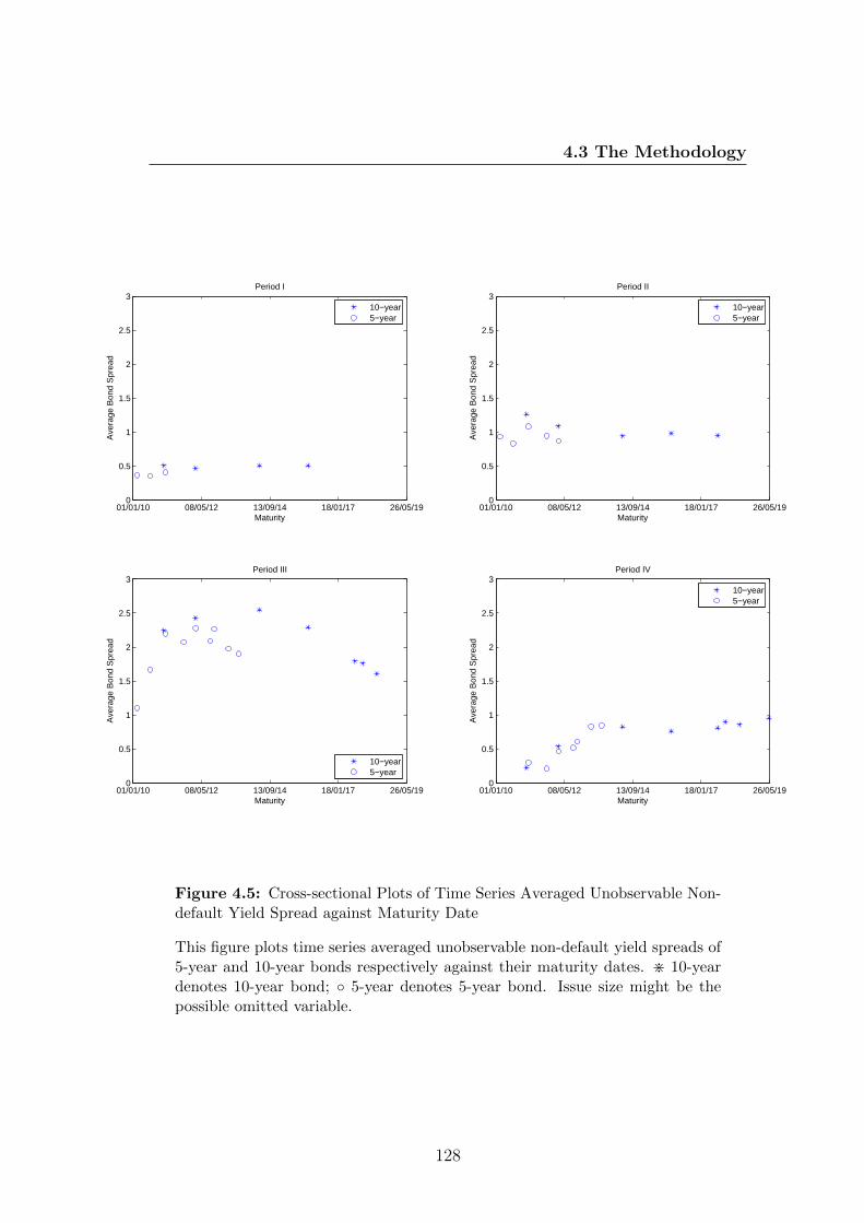
4.3 The Methodology
01/01/10 08/05/12 13/09/14 18/01/17 26/05/190
0.5
1
1.5
2
2.5
3
Maturity
Ave
rage
Bon
d S
prea
d
Period I
10−year5−year
01/01/10 08/05/12 13/09/14 18/01/17 26/05/190
0.5
1
1.5
2
2.5
3
Maturity
Ave
rage
Bon
d S
prea
d
Period II
10−year5−year
01/01/10 08/05/12 13/09/14 18/01/17 26/05/190
0.5
1
1.5
2
2.5
3
Maturity
Ave
rage
Bon
d S
prea
d
Period III
10−year5−year
01/01/10 08/05/12 13/09/14 18/01/17 26/05/190
0.5
1
1.5
2
2.5
3
Maturity
Ave
rage
Bon
d S
prea
d
Period IV
10−year5−year
Figure 4.5: Cross-sectional Plots of Time Series Averaged Unobservable Non-default Yield Spread against Maturity Date
This figure plots time series averaged unobservable non-default yield spreads of5-year and 10-year bonds respectively against their maturity dates. > 10-yeardenotes 10-year bond; 5-year denotes 5-year bond. Issue size might be thepossible omitted variable.
128

4.3 The Methodology
and recovered post the crisis. The liquidity conditions of the individual bonds
were quite different, as the standard deviations of the means of st in Period III
was 0.444, compared to 0.178 in Period IV.
Figure 4.6 plots the time series averages of st of the 5-year and 10-year bonds
respectively against their corresponding maturity dates for each bond and the
indicated sub-period. The illiquidity measure exhibited obvious seasoning effects
in all sub-periods except Period I where there were fewer observations. In par-
ticular, in Period III st was around four times as big for the most illiquid bond
compared to the most liquid bond. Our finding that seasoned bonds are more
illiquid than newly issued bonds and bonds close to maturity is consistent with
Schultz (2001) and Edwards & Piwowar (2007). Due to a flight-to-liquidity effect,
the plots in Period III had more curvature than those in other sub-periods, as
investors rebalance their portfolios towards more liquid securities. The volume
data in Figure 4.7 support that trading is more active just after the issuance as
well as before maturity.
Finally, as we want to explain non-default yield spreads as liquidity premia,
it is important to check their relation with the illiquidity measure. Figure 4.8
plots the time series averages of the unobservable non-default yield spreads of
the 5-year and 10-year bonds respectively against the time series averages of the
illiquidity measures for each bond and the indicated sub-period. The plots show
weak signs of a positive relationship between the non-default yield spread and the
illiquidity measure. However, this may result from omitting relevant variables,
such as issue sizes or time-to-maturities. We will further examine this relationship
in the next section.
We are also interested in the time series behaviour of both the default and
non-default components. Figure 4.9 gives a time series plot of both the daily
default component and the cross-sectionally averaged unobservable non-default
component in yield spreads. Before 26 July 2007, the non-default spread was
always above the default spread, and accounted for about 80% of the overall
spread. During the crisis (July 2007 - June 2009), the non-default component
accounted for about 48% of the overall spread on average. Its proportion dropped
to around 23% after the crisis (after June 2009). Between July 2007 and August
2008, there were four big jumps in both the default and non-default components,
129
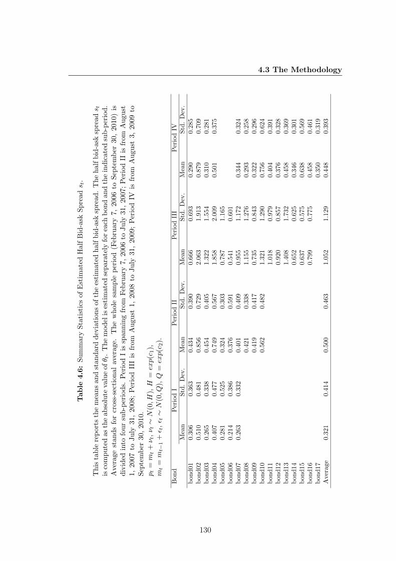
4.3 The MethodologyTable
4.6:
Su
mm
ary
Sta
tist
ics
ofE
stim
ated
Hal
fB
id-a
skS
pre
ads t
.
Th
ista
ble
rep
orts
the
mea
ns
and
stan
dar
dd
evia
tion
sof
the
esti
mat
edhal
fb
id-a
sksp
read
.T
he
hal
fb
id-a
sksp
read
s tis
com
pu
ted
asth
eab
solu
teva
lue
ofθ t
.T
he
mod
elis
esti
mat
edse
par
atel
yfo
rea
chb
ond
and
the
ind
icat
edsu
b-p
erio
d.
Ave
rage
stan
ds
for
cros
s-se
ctio
nal
aver
age.
Th
ew
hol
esa
mp
lep
erio
d(F
ebru
ary
7,20
06to
Sep
tem
ber
30,
2010
)is
div
ided
into
fou
rsu
b-p
erio
ds.
Per
iod
Iis
span
nin
gfr
omF
ebru
ary
7,20
06to
Ju
ly31
,20
07;
Per
iod
IIis
from
Au
gust
1,
2007
toJu
ly31,
200
8;
Per
iod
III
isfr
omA
ugu
st1,
2008
toJu
ly31
,20
09;
Per
iod
IVis
from
Au
gust
3,20
09to
Sep
tem
ber
30,
2010.
pt
=mt+ν t
,ν t∼N
(0,H
),H
=exp(c
1),
mt
=mt−
1+ε t
,ε t∼N
(0,Q
),Q
=exp(c
2).
Bon
dP
erio
dI
Per
iod
IIP
erio
dII
IP
erio
dIV
Mea
nS
td.
Dev
.M
ean
Std
.D
ev.
Mea
nS
td.
Dev
.M
ean
Std
.D
ev.
bon
d01
0.30
60.
363
0.43
40.3
90
0.6
66
0.6
93
0.2
90
0.2
85
bon
d02
0.51
00.
481
0.85
60.7
29
2.0
63
1.9
13
0.8
79
0.7
09
bon
d03
0.26
50.
338
0.45
40.4
05
1.3
22
1.5
54
0.3
10
0.2
81
bon
d04
0.40
70.
477
0.74
90.5
67
1.8
58
2.0
09
0.5
01
0.3
75
bon
d05
0.28
10.
525
0.32
40.3
03
0.7
87
1.1
65
bon
d06
0.21
40.
386
0.37
60.5
91
0.5
41
0.6
01
bon
d07
0.26
30.
332
0.40
10.4
09
0.9
55
1.1
72
0.3
44
0.3
24
bon
d08
0.42
10.3
38
1.1
55
1.2
76
0.2
93
0.2
58
bon
d09
0.41
90.4
17
0.7
35
0.8
43
0.3
22
0.2
96
bon
d10
0.56
20.4
82
1.3
21
1.2
90
0.7
56
0.6
24
bon
d11
1.0
18
0.9
79
0.4
04
0.3
91
bon
d12
0.9
20
0.8
57
0.3
76
0.3
28
bon
d13
1.4
08
1.7
32
0.4
58
0.3
69
bon
d14
0.6
52
0.6
25
0.3
46
0.3
01
bon
d15
0.6
37
0.5
75
0.6
38
0.5
69
bon
d16
0.7
99
0.7
75
0.4
58
0.4
61
bon
d17
0.3
50
0.3
19
Ave
rage
0.32
10.
414
0.50
00.4
63
1.0
52
1.1
29
0.4
48
0.3
93
130
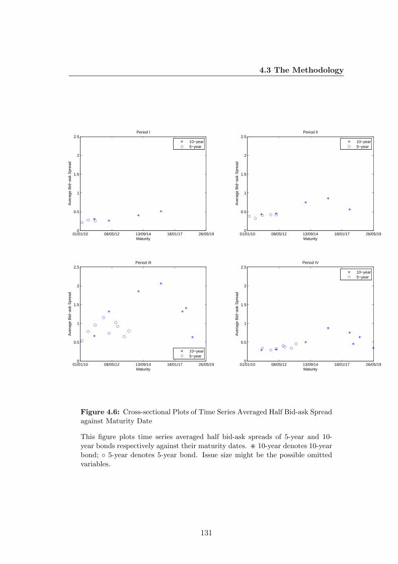
4.3 The Methodology
01/01/10 08/05/12 13/09/14 18/01/17 26/05/190
0.5
1
1.5
2
2.5
Maturity
Ave
rage
Bid
−as
k S
prea
d
Period I
10−year5−year
01/01/10 08/05/12 13/09/14 18/01/17 26/05/190
0.5
1
1.5
2
2.5
MaturityA
vera
ge B
id−
ask
Spr
ead
Period II
10−year5−year
01/01/10 08/05/12 13/09/14 18/01/17 26/05/190
0.5
1
1.5
2
2.5
Maturity
Ave
rage
Bid
−as
k S
prea
d
Period III
10−year5−year
01/01/10 08/05/12 13/09/14 18/01/17 26/05/190
0.5
1
1.5
2
2.5
Maturity
Ave
rage
Bid
−as
k S
prea
d
Period IV
10−year5−year
Figure 4.6: Cross-sectional Plots of Time Series Averaged Half Bid-ask Spreadagainst Maturity Date
This figure plots time series averaged half bid-ask spreads of 5-year and 10-year bonds respectively against their maturity dates. > 10-year denotes 10-yearbond; 5-year denotes 5-year bond. Issue size might be the possible omittedvariables.
131
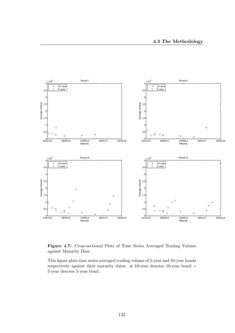
4.3 The Methodology
01/01/10 08/05/12 13/09/14 18/01/17 26/05/190
0.5
1
1.5
2
2.5
3
3.5
4x 10
4
Maturity
Ave
rage
Vol
ume
Period I
10−year5−year
01/01/10 08/05/12 13/09/14 18/01/17 26/05/190
0.5
1
1.5
2
2.5
3
3.5
4x 10
4
Maturity
Ave
rage
Vol
ume
Period II
10−year5−year
01/01/10 08/05/12 13/09/14 18/01/17 26/05/190
0.5
1
1.5
2
2.5
3
3.5
4x 10
4
Maturity
Ave
rage
Vol
ume
Period III
10−year5−year
01/01/10 08/05/12 13/09/14 18/01/17 26/05/190
0.5
1
1.5
2
2.5
3
3.5
4x 10
4
Maturity
Ave
rage
Vol
ume
Period IV
10−year5−year
Figure 4.7: Cross-sectional Plots of Time Series Averaged Trading Volumeagainst Maturity Date
This figure plots time series averaged trading volume of 5-year and 10-year bondsrespectively against their maturity dates. > 10-year denotes 10-year bond; 5-year denotes 5-year bond.
132
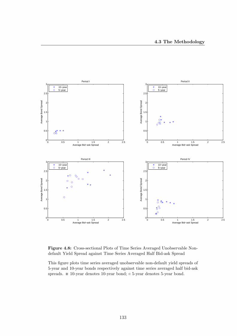
4.3 The Methodology
0 0.5 1 1.5 2 2.50
0.5
1
1.5
2
2.5
3
Average Bid−ask Spread
Ave
rage
Bon
d S
prea
d
Period I
10−year5−year
0 0.5 1 1.5 2 2.50
0.5
1
1.5
2
2.5
3
Average Bid−ask Spread
Ave
rage
Bon
d S
prea
d
Period II
10−year5−year
0 0.5 1 1.5 2 2.50
0.5
1
1.5
2
2.5
3
Average Bid−ask Spread
Ave
rage
Bon
d S
prea
d
Period III
10−year5−year
0 0.5 1 1.5 2 2.50
0.5
1
1.5
2
2.5
3
Average Bid−ask Spread
Ave
rage
Bon
d S
prea
d
Period IV
10−year5−year
Figure 4.8: Cross-sectional Plots of Time Series Averaged Unobservable Non-default Yield Spread against Time Series Averaged Half Bid-ask Spread
This figure plots time series averaged unobservable non-default yield spreads of5-year and 10-year bonds respectively against time series averaged half bid-askspreads. > 10-year denotes 10-year bond; 5-year denotes 5-year bond.
133
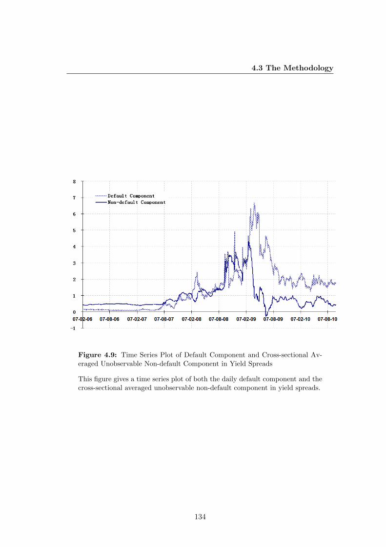
4.3 The Methodology
Figure 4.9: Time Series Plot of Default Component and Cross-sectional Av-eraged Unobservable Non-default Component in Yield Spreads
This figure gives a time series plot of both the daily default component and thecross-sectional averaged unobservable non-default component in yield spreads.
134

4.3 The Methodology
and each jump in the default component occurred ahead of each jump in the
non-default component. Between September 2008 and February 2009, both the
default and non-default components had sharp increases four times. By contrast,
they jumped almost at the same time. What is most surprising to us is that in
March 2009 the non-default component dropped sharply well before the default
component reached its historical highest point.1 After 2 March 2009 the default
component stayed well above the non-default component until the end of our
sample period. The non-default component fell below zero for a while during
June and July 2009.
1On February 23 2009, Citigroup announced that the United States government would takea 36% equity stake in the company by converting $25 billion in emergency aid into commonshares with a US treasury credit line of $45 billion.
135

4.4 Regression Results
4.4 Regression Results
Our sample consists of a cross-section of bonds, which allows us to examine
the connections amongst non-default yield spreads, our illiquidity measure and
various liquidity proxies. In particular, this enables us to answer the questions
that why bonds issued by a single company exhibit heterogenous levels of liquidity
and liquidity premia, how much of the time series variations are in common, and
how much are idiosyncratic. Therefore, we combine estimates over the whole
sample period to construct daily non-default yield spreads and the illiquidity
measure for each bond, and perform panel regressions on various liquidity proxies.
In doing this, it would be better to give some intuitive interpretation of the
liquidity proxies, their expected relationships with non-default yield spreads and
the illiquidity measure, and theoretical or empirical evidence.
4.4.1 Liquidity Proxies
Empirical papers, that examine liquidity in bond or equity markets, use both
direct measures (based on transaction data), and indirect measures (based on
bond characteristics and/or last prices). In our applications we will use both
direct and indirect measures, as they may provide different information about
bond liquidity.
The first proxy is the time-since-issue or time-to-maturity of a bond. The
intuition for these proxies is that traders buy bonds after the offering and sell
them shortly thereafter, as they expect that the bonds will get illiquid; while
bonds are close to maturity, some traders will start liquidating their holdings as
a result of imperfect match of maturities. Therefore, newly issued bonds and
bonds close to maturity may be more liquid than seasoned bonds. The difference
in the time-since-issue or time-to-maturity across bonds may explain the cross-
sectional difference in illiquidity and liquidity premia. Examining the corporate
bond market, Schultz (2001) find that newly issued bonds trade more than old
bonds. More recently, Edwards & Piwowar (2007) find, using transaction cost
estimates, that highly rated bonds, recently issued bonds, and bonds close to
maturity have lower transaction costs than do other bonds.
136

4.4 Regression Results
The second proxy is the issue amount of a bond. Intuitively, bonds with
smaller issue amount tend to get locked away by long-term investors more easily,
reducing the tradable amounts and thus their liquidity. Thus, the larger an issue,
the more liquid an bond is. Alexander et al. (2000) find that bond issues with
higher volume tend to be larger and more recently issued. Bao et al. (2011)
establish a robust connection between their illiquidity measure and liquidity-
related bond characteristics. Similarly, they find that the illiquidity measure is
higher for older and smaller bonds, and bonds with smaller average trade sizes
and higher idiosyncratic return volatilities. Not only these papers found strong
evidences of a seasoning effect, but also they both suggested that issue amounts
could be an indicator of bond liquidity.
Our third proxy is related to inventory holding costs. In microstructure litera-
ture, market makers’ inventory holding costs are often related to price volatilities.
Following Alexander et al. (2000), we use the average of absolute price returns to
approximate the volatility of fundamental prices.
The final three proxies are based on transaction level data and try to measure
trading frequencies. They are the daily turnover, the daily average trade size, and
the number of trades in a day of a bond. Obviously, all else equal, bonds which
trade more frequently will be more liquid. However, as they are constructed from
transaction-level data such as trading volumes, they do not tend to be forward-
looking, but rather reflect the current condition of market liquidity.
In addition to those measures of illiquidity, it would be interesting to look at
whether CDS spreads or the default risk will affect bond liquidity. There are good
reasons why they should be correlated. For example, when default probabilities
are high, it is plausible to believe that liquidity will be low, as there are fewer
buyers in the market willing to hold bonds with high default risk. Empirically,
Ericsson & Renault (2006) find evidence of a positive correlation between the
illiquidity and default components of bond yield spreads. Bao et al. (2011) also
find that bonds with higher CDS spreads are less liquid. However, it is important
to notice that CDS spreads are merely capturing the fundamental default risk,
rather than a measure of bond illiquidity.
Table 4.7 gives details on the definition of each liquidity proxy. It also shows
the expected relationship between each measure and the dependent variables,
137
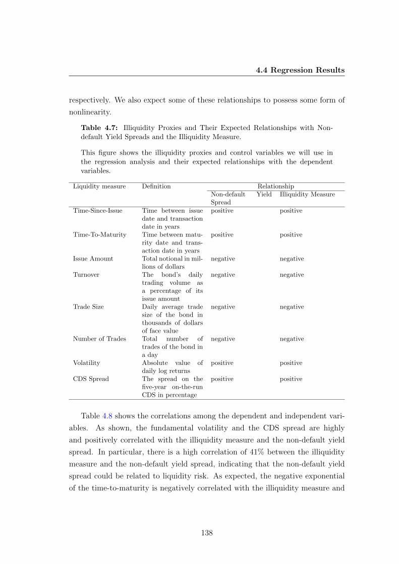
4.4 Regression Results
respectively. We also expect some of these relationships to possess some form of
nonlinearity.
Table 4.7: Illiquidity Proxies and Their Expected Relationships with Non-default Yield Spreads and the Illiquidity Measure.
This figure shows the illiquidity proxies and control variables we will use inthe regression analysis and their expected relationships with the dependentvariables.
Liquidity measure Definition RelationshipNon-default YieldSpread
Illiquidity Measure
Time-Since-Issue Time between issuedate and transactiondate in years
positive positive
Time-To-Maturity Time between matu-rity date and trans-action date in years
positive positive
Issue Amount Total notional in mil-lions of dollars
negative negative
Turnover The bond’s dailytrading volume asa percentage of itsissue amount
negative negative
Trade Size Daily average tradesize of the bond inthousands of dollarsof face value
negative negative
Number of Trades Total number oftrades of the bond ina day
negative negative
Volatility Absolute value ofdaily log returns
positive positive
CDS Spread The spread on thefive-year on-the-runCDS in percentage
positive positive
Table 4.8 shows the correlations among the dependent and independent vari-
ables. As shown, the fundamental volatility and the CDS spread are highly
and positively correlated with the illiquidity measure and the non-default yield
spread. In particular, there is a high correlation of 41% between the illiquidity
measure and the non-default yield spread, indicating that the non-default yield
spread could be related to liquidity risk. As expected, the negative exponential
of the time-to-maturity is negatively correlated with the illiquidity measure and
138
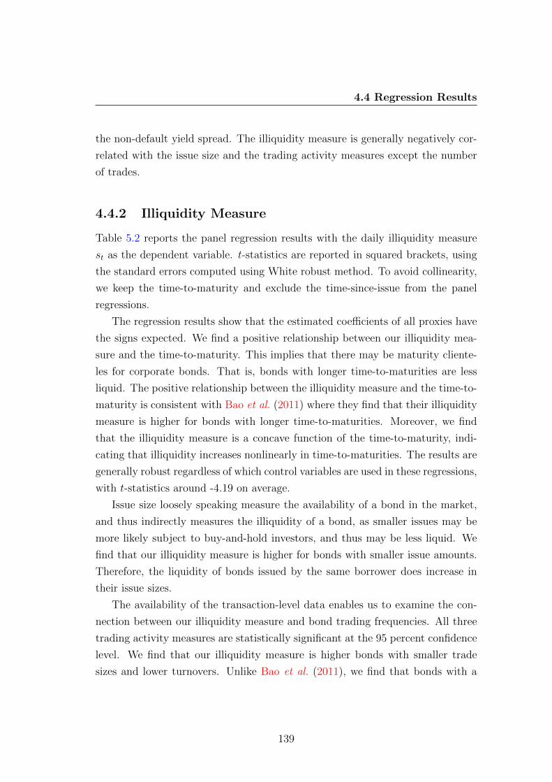
4.4 Regression Results
the non-default yield spread. The illiquidity measure is generally negatively cor-
related with the issue size and the trading activity measures except the number
of trades.
4.4.2 Illiquidity Measure
Table 5.2 reports the panel regression results with the daily illiquidity measure
st as the dependent variable. t-statistics are reported in squared brackets, using
the standard errors computed using White robust method. To avoid collinearity,
we keep the time-to-maturity and exclude the time-since-issue from the panel
regressions.
The regression results show that the estimated coefficients of all proxies have
the signs expected. We find a positive relationship between our illiquidity mea-
sure and the time-to-maturity. This implies that there may be maturity cliente-
les for corporate bonds. That is, bonds with longer time-to-maturities are less
liquid. The positive relationship between the illiquidity measure and the time-to-
maturity is consistent with Bao et al. (2011) where they find that their illiquidity
measure is higher for bonds with longer time-to-maturities. Moreover, we find
that the illiquidity measure is a concave function of the time-to-maturity, indi-
cating that illiquidity increases nonlinearly in time-to-maturities. The results are
generally robust regardless of which control variables are used in these regressions,
with t-statistics around -4.19 on average.
Issue size loosely speaking measure the availability of a bond in the market,
and thus indirectly measures the illiquidity of a bond, as smaller issues may be
more likely subject to buy-and-hold investors, and thus may be less liquid. We
find that our illiquidity measure is higher for bonds with smaller issue amounts.
Therefore, the liquidity of bonds issued by the same borrower does increase in
their issue sizes.
The availability of the transaction-level data enables us to examine the con-
nection between our illiquidity measure and bond trading frequencies. All three
trading activity measures are statistically significant at the 95 percent confidence
level. We find that our illiquidity measure is higher bonds with smaller trade
sizes and lower turnovers. Unlike Bao et al. (2011), we find that bonds with a
139
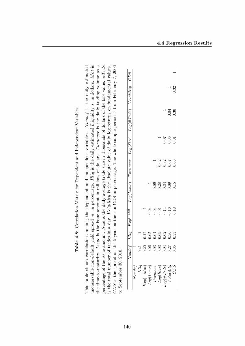
4.4 Regression Results
Table
4.8:
Corr
elat
ion
Mat
rix
for
Dep
enden
tan
dIn
dep
end
ent
Var
iab
les.
Th
ista
ble
show
sco
rrel
ati
ons
am
ong
the
dep
enden
tan
din
dep
end
ent
vari
able
s.Nondef
isth
ed
aily
esti
mat
edu
nob
serv
ab
len
on-d
efau
ltyie
ldsp
read
mt
inp
erce
nta
ge.Illiq
isth
ed
aily
esti
mat
edil
liqu
idit
ys t
indol
lars
.Mat
isth
eti
me-
to-m
atu
rity
.Issue
isth
eis
sue
amou
nt
inm
illion
sof
dol
lars
.Turnover
isth
ed
aily
trad
ing
volu
me
asa
per
centa
ge
of
the
issu
eam
ount.Size
isth
ed
aily
aver
age
trad
esi
zein
thou
san
ds
ofd
olla
rsof
the
face
valu
e.#Trds
isth
eto
tal
nu
mb
erof
trad
esin
aday
.Volalility
isth
eab
solu
teva
lue
ofd
aily
log
retu
rns
onfu
nd
amen
tal
valu
es.
CDS
isth
esp
read
on
the
5-ye
aron
-th
e-ru
nC
DS
inp
erce
nta
ge.
Th
ew
hol
esa
mp
lep
erio
dis
from
Feb
ruar
y7,
2006
toS
epte
mb
er30,
201
0.
Nondef
Illiq
Exp(−
Mat)
Log
(Issue)
Turnover
Log
(Size)
Log
(#Trds)
Volatility
CDS
Nondef
1Illiq
0.41
1Exp(−Mat)
-0.2
0-0
.12
1Log
(Issue)
0.06
-0.0
5-0
.04
1Turnover
-0.0
3-0
.04
0.04
0.0
91
Log
(Size)
-0.0
3-0
.09
-0.0
10.2
80.6
21
Log
(#Trds)
0.04
0.02
0.14
0.3
40.3
20.0
71
Volatility
0.27
0.36
-0.1
60.0
90.0
70.0
60.0
41
CDS
0.35
0.33
0.18
0.1
50.0
60.0
10.3
00.3
21
140

4.4 Regression Results
Table 4.9: Regression of the Illiquidity Measure on Illiquidity and CreditProxies.
This table reports the panel regressions with the daily illiquidity measure st asthe dependent variable. t-statistics are reported in square brackets using Whiterobust method. The daily illiquidity measure is in dollars. Mat is the time-to-maturity in years. Issue is the issue amount in millions of dollars. Turnoveris the daily trading volume as a percentage of the issue amount. Size is thedaily average trade size in thousands of dollars of the face value. #Trds is thetotal number of trades in a day. Nondef is the daily estimated unobservablenon-default yield spread in percentage. V olatility is the absolute value of dailylog returns on the fundamental price in percentage. CDS is the spread on the 5-year on-the-run CDS in percentage. The whole sample period is from February7, 2006 to September 30, 2010.
Coefficients on equations(1) (2) (3) (4) (5) (6) (7)
Cons 0.18** 1.94** 2.03** 1.96** 1.92** 1.92** 1.68**[3.20] [2.46] [3.27] [3.19] [3.25] [2.98] [2.65]
Exp(−Mat) -1.33** -1.01** -0.97** -0.99** -0.98** -0.32**[-4.43] [-4.09] [-4.08] [-3.87] [-4.46] [-2.14]
Log(Issue) -0.23** -0.25** -0.23** -0.21** -0.22** -0.22**[-2.15] [-2.97] [-2.87] [-2.72] [-2.53] [-2.57]
Turnover -7.24**[-6.24]
Log(Size) -0.03**[-4.90]
Log(#Trds) -0.04**[-2.29]
Nondef 0.23**[6.12]
V olatility 0.36** 0.34** 0.34** 0.34** 0.33** 0.28**[6.53] [6.56] [6.70] [6.74] [6.66] [6.13]
CDS 0.17** 0.24** 0.19** 0.19** 0.19** 0.20** 0.12**[5.56] [7.49] [6.53] [6.62] [6.56] [6.57] [6.23]
Obs 10206 13186 10196 10183 10184 10195 10196R2 17.57% 15.12% 20.50% 21.02% 21.24% 20.52% 26.43%
141

4.4 Regression Results
larger number of trades have smaller bid-ask spreads and are more liquid. Alter-
natively stated, more trades do lead to more liquidity. However, despite they are
statistically significant, their contributions to R2 appear to be modest. Adding
the turnover, the trade size and the number of trades only increases R2 by 0.52%,
0.74% and 0.02%, respectively.
In addition, we find that, after controlling for the time-to-maturity, the issue
size, the fundamental volatility and the other variables, our illiquidity measure
is positively correlated with the CDS spread. That is, the more likely the com-
pany will default, the less liquid its bonds become. The connection in terms of
magnitude and statistical significance is very strong as the t-statistics are about
6.57 on average. If the CDS spread increases by 1 percent, our illiquidity measure
would increase roughly about 19 percent which is sizeable given that the average
illiquidity measure before the crisis was only at 32.1 percent. However, the result
does not mean that CDS spreads contain any information on bond liquidity. This
is merely because that during distressed time there are fewer investors willing to
hold bonds with high default risk. Our result also confirms the finding in Ericsson
& Renault (2006) and Bao et al. (2011) that there is a close relationship between
credit and liquidity risks.
Interestingly, the absolute returns of the fundamental price as a proxy for price
uncertainty is found to be positively correlated with the illiquidity measure. It
is well-known that market makers’ inventory costs are higher if price uncertainty
is higher. An important source of uncertainty is related to the predictability of
future price movements. Thus, a higher price uncertainty leads to larger bid-ask
spreads, and thus lower liquidity. In addition, the non-default yield spread also
has some predictability for the illiquidity measure. Including the non-default
yield spread in the regression increases the R2 by 5.93%.
Finally, among the independent variables, some of them are common across
the bonds, such as the fundamental volatility and the CDS spread. Others are
viewed as the idiosyncratic factors, for instance, the time-to-maturity, the issue
size and the trading activity measures. The fundamental volatility and the CDS
spread all together can explain 17.57% of the variations in the illiquidity mea-
sure, in which 5.38% is attributable to the fundamental volatility. Adding the
142

4.4 Regression Results
idiosyncratic factors such as the time-to-maturity, the issue size and the non-
default yield spread increase the R2 by 8.86%. The contribution of the trading
activity measures to the R2 appears to be modest (less than 1%). It is important
to caution that the variations which are unexplained by our selected factors may
include the errors which are introduced in the process of separating the default
and non-default price components as well as estimating the illiquidity measure
and the non-default yield spread.
4.4.3 Non-default Yield Spread
Now we focus on the variations in the non-default component of the yield spreads.
Once again we regress the non-default yield spreads of the individual bonds on a
number of liquidity proxies and control variables. Table 4.10 reports the regres-
sion results.
As many studies explain non-default yield spreads as a liquidity premium
which is the compensation required by investors for the transaction costs in-
curred when trading the assets, it is important to check whether there is a strong
relationship between the non-default yield spread and the illiquidity measure.
Table 4.10 shows that the non-default yield spread is significantly and positively
related to the illiquidity measure. Thus, the size of the non-default yield spread
increases, while the liquidity of a bond decreases. This is consistent with the hy-
pothesis that illiquid bonds have larger liquidity premia embedded within their
yield spreads than liquid bonds. In particular, the regression coefficient on the
illiquidity measure is 0.06 with a t-statistic of 17.62. This means that for two
bonds issued by the company a difference of $1.0 in the illiquidity measure leads to
a difference of 6 bps in the yield spread. This is obviously much smaller than the
differences found in Longstaff et al. (2005) (a difference of 36.9% for AAA/AA-
rated firms) and Chen et al. (2007) (42% for Investment Grade bonds). This is
possibly because our analysis is limited to a set of single A-rated bonds, issued
by a specific company, and our sample (from February 2006 to September 2010)
is more recent than the one used in Longstaff et al. (2005) (from March 2001 to
October 2002) and Chen et al. (2007) (from 1995 to 2003).
143
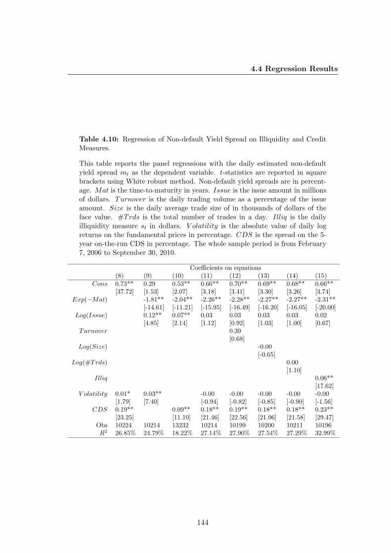
4.4 Regression Results
Table 4.10: Regression of Non-default Yield Spread on Illiquidity and CreditMeasures.
This table reports the panel regressions with the daily estimated non-defaultyield spread mt as the dependent variable. t-statistics are reported in squarebrackets using White robust method. Non-default yield spreads are in percent-age. Mat is the time-to-maturity in years. Issue is the issue amount in millionsof dollars. Turnover is the daily trading volume as a percentage of the issueamount. Size is the daily average trade size of in thousands of dollars of theface value. #Trds is the total number of trades in a day. Illiq is the dailyilliquidity measure st in dollars. V olatility is the absolute value of daily logreturns on the fundamental prices in percentage. CDS is the spread on the 5-year on-the-run CDS in percentage. The whole sample period is from February7, 2006 to September 30, 2010.
Coefficients on equations(8) (9) (10) (11) (12) (13) (14) (15)
Cons 0.73** 0.29 0.53** 0.66** 0.70** 0.69** 0.68** 0.66**[37.72] [1.53] [2.07] [3.18] [3.41] [3.30] [3.26] [3.74]
Exp(−Mat) -1.81** -2.04** -2.26** -2.28** -2.27** -2.27** -2.31**[-14.61] [-11.21] [-15.95] [-16.49] [-16.20] [-16.05] [-20.00]
Log(Issue) 0.12** 0.07** 0.03 0.03 0.03 0.03 0.02[4.85] [2.14] [1.12] [0.92] [1.03] [1.00] [0.67]
Turnover 0.39[0.68]
Log(Size) -0.00[-0.65]
Log(#Trds) 0.00[1.10]
Illiq 0.06**[17.62]
V olatility 0.01* 0.03** -0.00 -0.00 -0.00 -0.00 -0.00[1.79] [7.40] [-0.94] [-0.82] [-0.85] [-0.90] [-1.56]
CDS 0.19** 0.09** 0.18** 0.19** 0.18** 0.18** 0.23**[23.25] [11.10] [21.46] [22.56] [21.96] [21.58] [29.47]
Obs 10224 10214 13232 10214 10199 10200 10211 10196R2 26.85% 24.79% 18.22% 27.14% 27.90% 27.54% 27.29% 32.99%
144
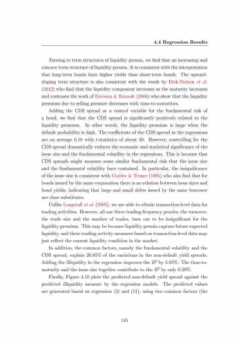
4.4 Regression Results
Turning to term structures of liquidity premia, we find that an increasing and
concave term structure of liquidity premia. It is consistent with the interpretation
that long-term bonds have higher yields than short-term bonds. The upward-
sloping term structure is also consistent with the result by Dick-Nielsen et al.
(2012) who find that the liquidity component increases as the maturity increases
and contrasts the work of Ericsson & Renault (2006) who show that the liquidity
premium due to selling pressure decreases with time-to-maturities.
Adding the CDS spread as a control variable for the fundamental risk of
a bond, we find that the CDS spread is significantly positively related to the
liquidity premium. In other words, the liquidity premium is large when the
default probability is high. The coefficients of the CDS spread in the regressions
are on average 0.18 with t-statistics of about 20. However, controlling for the
CDS spread dramatically reduces the economic and statistical significance of the
issue size and the fundamental volatility in the regressions. This is because that
CDS spreads might measure some similar fundamental risk that the issue size
and the fundamental volatility have contained. In particular, the insignificance
of the issue size is consistent with Crabbe & Truner (1995) who also find that for
bonds issued by the same corporation there is no relation between issue sizes and
bond yields, indicating that large and small debts issued by the same borrower
are close substitutes.
Unlike Longstaff et al. (2005), we are able to obtain transaction-level data for
trading activities. However, all our three trading frequency proxies, the turnover,
the trade size and the number of trades, turn out to be insignificant for the
liquidity premium. This may be because liquidity premia capture future expected
liquidity, and these trading activity measures based on transaction-level data may
just reflect the current liquidity condition in the market.
In addition, the common factors, namely the fundamental volatility and the
CDS spread, explain 26.85% of the variations in the non-default yield spreads.
Adding the illiquidity in the regression improves the R2 by 5.85%. The time-to-
maturity and the issue size together contribute to the R2 by only 0.29%.
Finally, Figure 4.10 plots the predicted non-default yield spread against the
predicted illiquidity measure by the regression models. The predicted values
are generated based on regression (3) and (11), using two common factors (the
145
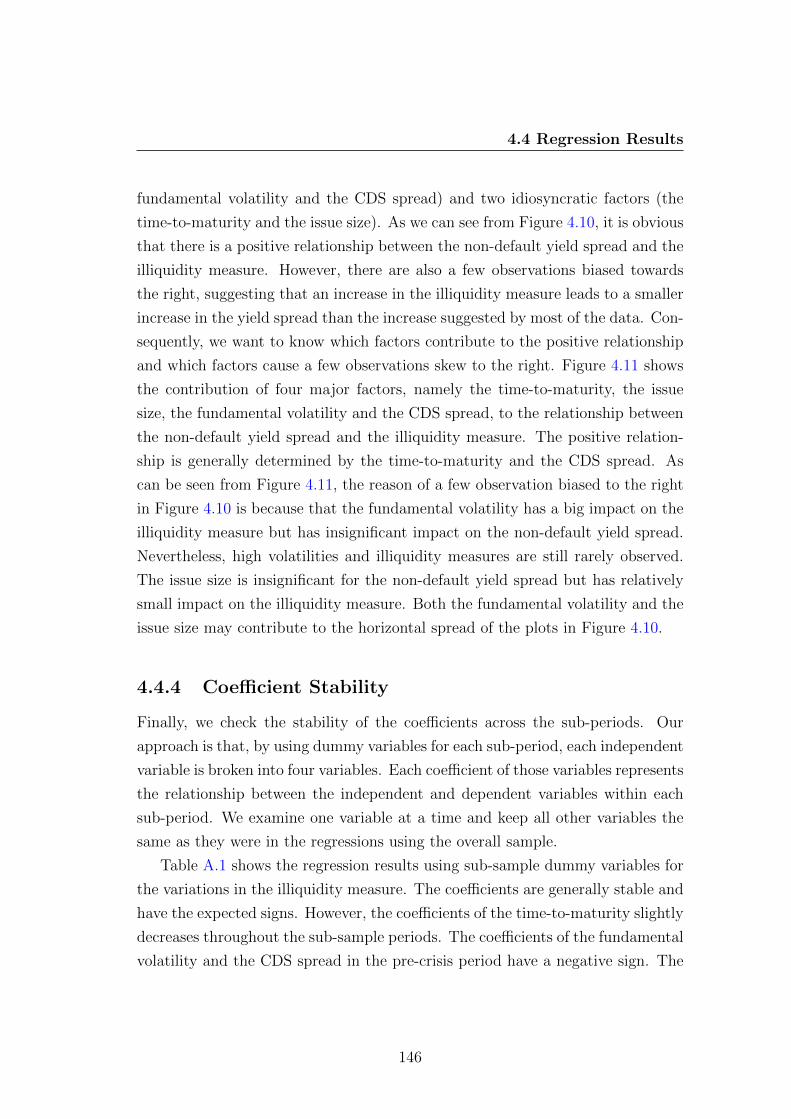
4.4 Regression Results
fundamental volatility and the CDS spread) and two idiosyncratic factors (the
time-to-maturity and the issue size). As we can see from Figure 4.10, it is obvious
that there is a positive relationship between the non-default yield spread and the
illiquidity measure. However, there are also a few observations biased towards
the right, suggesting that an increase in the illiquidity measure leads to a smaller
increase in the yield spread than the increase suggested by most of the data. Con-
sequently, we want to know which factors contribute to the positive relationship
and which factors cause a few observations skew to the right. Figure 4.11 shows
the contribution of four major factors, namely the time-to-maturity, the issue
size, the fundamental volatility and the CDS spread, to the relationship between
the non-default yield spread and the illiquidity measure. The positive relation-
ship is generally determined by the time-to-maturity and the CDS spread. As
can be seen from Figure 4.11, the reason of a few observation biased to the right
in Figure 4.10 is because that the fundamental volatility has a big impact on the
illiquidity measure but has insignificant impact on the non-default yield spread.
Nevertheless, high volatilities and illiquidity measures are still rarely observed.
The issue size is insignificant for the non-default yield spread but has relatively
small impact on the illiquidity measure. Both the fundamental volatility and the
issue size may contribute to the horizontal spread of the plots in Figure 4.10.
4.4.4 Coefficient Stability
Finally, we check the stability of the coefficients across the sub-periods. Our
approach is that, by using dummy variables for each sub-period, each independent
variable is broken into four variables. Each coefficient of those variables represents
the relationship between the independent and dependent variables within each
sub-period. We examine one variable at a time and keep all other variables the
same as they were in the regressions using the overall sample.
Table A.1 shows the regression results using sub-sample dummy variables for
the variations in the illiquidity measure. The coefficients are generally stable and
have the expected signs. However, the coefficients of the time-to-maturity slightly
decreases throughout the sub-sample periods. The coefficients of the fundamental
volatility and the CDS spread in the pre-crisis period have a negative sign. The
146

4.4 Regression Results
Figure 4.10: Scatter Plots of Predicted Non-default Yield Spread againstPredicted Illiquidity Measure
This figure plots the predicted non-default yield spread against the predictedilliquidity measure. The predicted values are generated based on the tworegressions:
Nondef = α+ β1Exp(−Mat) + β2Log(Issue) + β3V olatility + β4CDS + ε
and
Illiq = α′ + β′1Exp(−Mat) + β′2Log(Issue) + β′3V olatility + β′4CDS + ε′
where Mat is the time-to-maturity in years, Issue is the issue amountin millions of dollars, V olatility is the absolute value of daily log returns on thefundamental prices in percentage, CDS is the spread on the 5-year on-the-runCDS in percentage, Illiq is the daily illiquidity measure st in dollars andNondef is the daily estimated unobservable non-default yield spread mt inpercentage. The figure suggests a positive relation between the non-defaultyield spread and the illiquidity measure.
147

4.4 Regression Results
Figure 4.11: Contribution of Major Factors to the Relation between the Non-default Yield Spread and the Illiquidity Measure
This figure shows the contribution of the four major factors, namely the time-to-maturity, the issue size, the fundamental volatility and the CDS spread,to the relationship between the non-default yield spread and the illiquiditymeasure. The figure is constructed based on the coefficients estimated fromthe two regressions:
Nondef = α+ β1Exp(−Mat) + β2Log(Issue) + β3V olatility + β4CDS + ε
and
Illiq = α′ + β′1Exp(−Mat) + β′2Log(Issue) + β′3V olatility + β′4CDS + ε′,
where Mat is the time-to-maturity in years, Issue is the issue amountin millions of dollars, V olatility is the absolute value of daily log returnson the fundamental prices in percentage, CDS is the spread on the 5-yearon-the-run CDS in percentage, Illiq is the daily illiquidity measure st in dollarsand Nondef is the daily estimated unobservable non-default yield spreadmt in percentage. The figure suggests that the positive relationship betweenthe non-default yield spread and the illiquidity measure is mainly due to thetime-to-maturity and the CDS spread.
148

4.4 Regression Results
coefficient of the turnover in Period III has the largest magnitude. Both the trade
size and the number of trades are insignificant in Period III.
In Table A.2 the coefficients in the non-default yield spread regression show a
sign of slight instability. The coefficient of time-to-maturity in Period I is dramat-
ically smaller than those in other periods. The issue size becomes insignificant in
Period II and IV and has a negative coefficient in Period I. Coefficients of both
the fundamental volatility and the CDS spread have positive signs only in Period
III. Coefficients of the illiquidity measure in Period I and IV have negative signs.
We expect some variations in the coefficients across different sub-periods.
However, the overall sample is more suitable for our purpose as we generally try
to associate the variations in the illiquidity measure and the non-default yield
spread with various liquidity proxies.
149
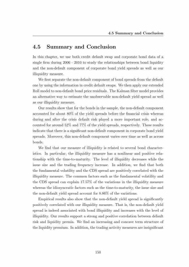
4.5 Summary and Conclusion
4.5 Summary and Conclusion
In this chapter, we use both credit default swap and corporate bond data of a
single firm during 2006 - 2010 to study the relationships between bond liquidity
and the non-default component of corporate bond yield spreads as well as our
illiquidity measure.
We first separate the non-default component of bond spreads from the default
one by using the information in credit default swaps. We then apply our extended
Roll model to non-default bond price residuals. The Kalman filter model provides
an alternative way to estimate the unobservable non-default yield spread as well
as our illiquidity measure.
Our results show that for the bonds in the sample, the non-default component
accounted for about 80% of the yield spreads before the financial crisis whereas
during and after the crisis default risk played a more important role, and ac-
counted for around 52% and 77% of the yield spreads, respectively. These results
indicate that there is a significant non-default component in corporate bond yield
spreads. Moreover, this non-default component varies over time as well as across
bonds.
We find that our measure of illiquidity is related to several bond character-
istics. In particular, the illiquidity measure has a nonlinear and positive rela-
tionship with the time-to-maturity. The level of illiquidity decreases while the
issue size and the trading frequency increase. In addition, we find that both
the fundamental volatility and the CDS spread are positively correlated with the
illiquidity measure. The common factors such as the fundamental volatility and
the CDS spread can explain 17.57% of the variations in the illiquidity measure
whereas the idiosyncratic factors such as the time-to-maturity, the issue size and
the non-default yield spread account for 8.86% of the variations.
Empirical results also show that the non-default yield spread is significantly
positively correlated with our illiquidity measure. That is, the non-default yield
spread is indeed associated with bond illiquidity and increases with the level of
illiquidity. Our results support a strong and positive correlation between default
risk and liquidity premia. We find an increasing and concave term structure of
the liquidity premium. In addition, the trading activity measures are insignificant
150

4.5 Summary and Conclusion
for the liquidity premium, suggesting that the liquidity premium may reflect
future expected illiquidity of a bond. Finally, 26.85% of the variations in the
liquidity premium is explained by the common factors, such as the CDS spread
and the fundamental volatility. The illiquidity measure is the most influential
idiosyncratic factor of the liquidity premium. Including the illiquidity measure
increases the R2 by 5.85%.
Our main analysis is based on the assumption that CDS spreads do not contain
a liquidity premium. However, if they do then it will create a common factor
(across bonds of similar maturity) in the residuals. Reduced but still significant
liquidity effects would then be estimated. It is also important to caution that
our results may not generalize to other bonds or other firms. There may be some
doubt about our results for the broader market of corporate bonds. In our future
research, we may extend our data set to include a larger number of corporate
bonds. Still, for the bonds that we analyzed, these results do suggest that there
is a significant non-default component in the corporate bond yield spread which is
associated with the illiquidity of a bond, and the illiquidity and liquidity premia
vary over time and across bonds deriving by both common and idiosyncratic
factors.
151

Chapter 5
An Equilibrium Model of
Liquidity in Bond Markets
5.1 Introduction
The recent financial crisis has revealed a strong need to gain a better understand-
ing of the influence of illiquidity on asset pricing. In particular, the illiquidity of
bond markets has captured the interest of researchers, practitioners, and policy
makers. Many empirical studies have found that very similar assets can exhibit
significantly different levels of liquidity.1 Therefore, fundamental asset pricing
questions have to be asked: why similar assets differ significantly in liquidity, and
in particular, why some bonds are more liquid and more expensive (in terms of
price) than other (otherwise identical) bonds.
1Amihud & Mendelson (1991) compare the yields on short-term U.S. Treasury notes andbills with the same maturities, and find that their liquidity is different. Krishnamurthy (2002)documents that on-the-run Treasury bonds are significantly more liquid than off-the-run bondsmaturing on nearby dates. In fact, one of long term capital management’s (LTCM) mainstrategies was to exploit the price differences between on-the-run and off-the-run Treasurybonds. Krishnamurthy & Vissing-Jorgensen (2012) examine the yield differences between 6-month Federal Deposit Insurance Corporation (FDIC) insured certificates of deposit (CDs) and6-month Treasury bills. They suggest that, given FDIC insurance, the yield differences canonly be due to liquidity.
152

5.1 Introduction
To answer the questions, a “partial equilibrium” analysis that imposes ex
ante assumptions on the liquidity of assets will be inappropriate. Some models
previously developed assume exogenously given transaction costs, the liquidity
differentials are explained by exogenously pre-specified differences in transac-
tion costs.1 In contrast, in this paper we characterize an equilibrium model
in which the heterogeneity of liquidity among bonds is determined endogenously,
and thereby, we focus on understanding how liquidity externalities arise in an
equilibrium framework.
Different from search-based models, our model assumes that a number of
(otherwise identical) bonds are exchanged amongst the market participants: a
set of risk neutral investors, with exogenously determined cash flow constraints
and having in mind their desire and ability to liquidate a proportion of their
bonds in a future date prior to maturity as they may experience liquidity shocks
or face surprise investment opportunities, purchase the bonds by maximizing
their post-investment residual surplus; another set of risk neutral traders, who
are willing to buy the bonds unwound by the former investors, come to the
marketplace randomly; a single risk averse competitive market maker acts as the
whole financial intermediaries by bridging the gaps between buyers and sellers
and requires a premium to cover expected inventory-holding costs when supplying
immediacy.23
1See, for example, Amihud & Mendelson (1986), Huang (2003), Vayanos & Vila (1999) andVayanos (1998).
2Economides & Siow (1988) using search-based model show that agents prefer to trade in aspot market with high rather than low liquidity. Vayanos & Wang (2007) develop a search-basedmodel in which investors of different horizons can invest in two assets with identical payoffs.They show that there exist such an equilibrium where all short-term investors search for thesame asset. Weill (2008) show that although the search technology is the same for all assets,heterogeneous trading costs arise endogenously. Vayanos & Weill (2008) use search-based modelto explain the on-the-run phenomenon.
3Another strand of market microstructure literature (e.g. Grossman (1980), Kyle (1985),Brennan & Subrahmanyam (1996), and Easley et al. (1996).) suggests that asymmetric infor-mation creates significant illiquidity costs. Our study focuses on inventory-holding risk facedby dealers in bond markets for the following reason. Main investors in corporate bond mar-kets are institutional investors such as pension funds and insurance companies whose long termobligations can be matched reasonably well to the relatively predictable, long term stream ofcoupon interest payments generated by bonds. As a result, most or all of a bond issue is oftenabsorbed into stable ‘buy-and-hold’ portfolios soon after issue. When pension funds or insur-ance companies liquidate, they liquidate for cash, rather than short term trades motivated byasymmetric information.
153
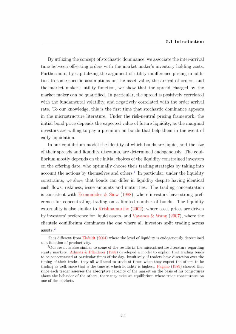
5.1 Introduction
By utilizing the concept of stochastic dominance, we associate the inter-arrival
time between offsetting orders with the market maker’s inventory holding costs.
Furthermore, by capitalizing the argument of utility indifference pricing in addi-
tion to some specific assumptions on the asset value, the arrival of orders, and
the market maker’s utility function, we show that the spread charged by the
market maker can be quantified. In particular, the spread is positively correlated
with the fundamental volatility, and negatively correlated with the order arrival
rate. To our knowledge, this is the first time that stochastic dominance appears
in the microstructure literature. Under the risk-neutral pricing framework, the
initial bond price depends the expected value of future liquidity, as the marginal
investors are willing to pay a premium on bonds that help them in the event of
early liquidation.
In our equilibrium model the identity of which bonds are liquid, and the size
of their spreads and liquidity discounts, are determined endogenously. The equi-
librium mostly depends on the initial choices of the liquidity constrained investors
on the offering date, who optimally choose their trading strategies by taking into
account the actions by themselves and others.1 In particular, under the liquidity
constraints, we show that bonds can differ in liquidity despite having identical
cash flows, riskiness, issue amounts and maturities. The trading concentration
is consistent with Economides & Siow (1988), where investors have strong pref-
erence for concentrating trading on a limited number of bonds. The liquidity
externality is also similar to Krishnamurthy (2002), where asset prices are driven
by investors’ preference for liquid assets, and Vayanos & Wang (2007), where the
clientele equilibrium dominates the one where all investors split trading across
assets.2
1It is different from Eisfeldt (2004) where the level of liquidity is endogenously determinedas a function of productivity.
2Our result is also similar to some of the results in the microstructure literature regardingequity markets. Admati & Pfleiderer (1988) developed a model to explain that trading tendsto be concentrated at particular times of the day. Intuitively, if traders have discretion over thetiming of their trades, they all will tend to trade at times when they expect the others to betrading as well, since that is the time at which liquidity is highest. Pagano (1989) showed thatsince each trader assesses the absorptive capacity of the market on the basis of his conjecturesabout the behavior of the others, there may exist an equilibrium where trade concentrates onone of the markets.
154

5.1 Introduction
When the quantity of bonds which do trade implies that there are some trad-
able and non-tradable bonds, the identity of the ones which are traded may result
from a ‘Sunspot’ equilibrium where it is optimal for traders to randomly label a
subset of the bonds as the liquid ones and concentrate trading on them.1 This
self-fulfilling prophecy is analogous to the on-the-run phenomenon where expect-
ing lower liquidity will themselves reduce liquidity.
The difference between our paper and the previous studies is that we relate
liquidity demands to liquidity conditions. Our model predicts that liquidity con-
ditions of investors may affect their liquidity demand, and thereby, prices and
spreads. The increase of liquid asset holdings can be the result of forwarding
looking investors shifting their preferences towards liquid assets, ahead of periods
when liquidity is in shortage. Alternatively, the investors with loose liquidity
constraints holding more illiquid bonds can be interpreted as long-term investors,
whereas the agents with tough liquidity constraints holding more liquid bonds
can be interpreted as short-term investors. This clientele effect is consistent with
Vayanos & Vila (1999) where they show that agents with short investment hori-
zon buy the liquid asset and agents with long investment horizon hold the illiquid
asset.
Our study contributes the existing literature in several ways. First, in pre-
vious theoretical studies of asset pricing, ex ante assumptions on asset liquidity
are normally made.2 Our study bridges the gap by characterizing an equilib-
1Market uncertainty can also be driven by extrinsic uncertainty, which includes such vari-ables as market psychology, self-fulfilling prophecies and ‘animal spirits’ (Keynes (1936)), col-lectively known as ‘sunspots’. The concept of ‘sunspot’ equilibrium was introduced by Cass& Shell (1983). Duffy (2005) interpret Sunspot equilibrium as a means of coordinating theexpectations and plans of market participants. For applications of ‘Sunspots’ equilibrium infinance, see Diamond (1983) and Peck & Shell (2003).
2Acharya & Pedersen (2005) derive an equilibrium model under exogenous stochastic trans-action costs. Amihud & Mendelson (1986) analyze a model in which investors with differentexpected holding periods trade assets with different relative spreads, which are pre-determined.To jointly explain the equity premium and the low risk-free rate, Aiyagari & Gertler (1991)introduce two kinds of securities in their model. One type of security is freely exchanged, whilethe other type is costly to trade. By assuming that one asset is liquid while the other assetcarries proportional transaction costs, Vayanos & Vila (1999) show that agents buy the liquidasset for short-term investment and the illiquid asset for long-term investment. In other words,there is a well-defined clientele for each asset. More recently, Huang (2003) shows that in equi-librium, by comparing the illiquid bond with the (otherwise identical) liquid bond, the illiquidbond should generate a higher expected return to compensate its holders.
155
5.1 Introduction
rium model in which the heterogeneity of liquidity among bonds is determined
endogenously. Second, our model, which is not search-based, offers an alternative
theory that explains why similar assets exhibits heterogenous levels of liquidity.
Third, by utilizing the concepts of stochastic dominance, utility indifference pric-
ing plus some specific assumptions on the asset value, the arrival of orders, the
market maker’s utility function and agents’ risk neutrality, the equilibrium bond
prices and spreads can be quantified.1 Forth, we show that the identity of which
bonds do trade can be a result of a ‘Sunspot’ equilibrium. Fifth, our model shows
that forward looking investors’ liquidity preference is affected by their liquidity
conditions.
Among microstructure studies on liquidity, Foucault et al. (2005) develop a
dynamic model of a limit order market in which agents are strategic and take
liquidity into account when trading. Their model predicts a negative relationship
between the order arrival rate and the market resiliency. Rosu (2009) models an
order-driven market where strategic traders tradeoff execution prices and waiting
costs. The model predicts that higher trading activity and higher trading com-
petition cause smaller spreads and lower price impact. Our model shares some
features of these models, moreover, complements this strand of microstructure
literature.
The rest of the chapter is structured as follows. Section 2 gives the intro-
duction and discussion of the general model, followed by a specific example. In
Section 3, we characterize the equilibrium. Then, we analyze the quantitative
implications of the equilibrium in Section 4. Section 5 concludes.
1Hodges & Neuberger (1989) were the first to introduce the concept of utility indifferencepricing in the context of option pricing under transaction costs in Black-Scholes model.
156

5.2 The General Model
5.2 The General Model
In this section, we introduce the general model, and provide the motivation,
the discussion of the model, and especially the behaviors of different market
participants.
5.2.1 Financial Market
The economy has three dates, 0, 1 and 2. The financial market consists of a
single consumption good, which is used as the numeraire, and N bonds, indexed
by j ∈ N = 1, 2, . . . , N.1 We assume:
(A) All the bonds issued on date 0 and maturing on date 2 has a face value of
1 dollar.2
(B) The total supply of the bonds is K, with the supply of bond j in terms of
dollar value, denoted kj (that is,∑N
j=1 kj = K, 0 < kj).
(C) All the bonds share the same level of default risk (i.e. perfectly correlated
defaults).3
One unique feature of our setup is that in contrast to previous literature we
do not impose ex ante assumptions on bond liquidity.4 The heterogenous levels
of liquidity can be determined endogenously by interactions among traders.
5.2.2 Agents
We consider a dealership market where there are three types of market partici-
pants trading the bonds, namely Type 1 trader, Type 2 trader and the market
maker. The following assumptions are made:
1Equivalently, one dollar one consumption good.2The analysis ignores coupons. It applies with coupons if all bonds pay the same coupon
rate.3Imperfectly correlated defaults are likely to change our results. However, perfectly corre-
lated defaults are suitable for our purpose, as we try to explain that why otherwise identicalbonds (e.g. bonds issued by a single company) differ in their liquidity.
4See, for example, Amihud & Mendelson (1986), Huang (2003), Vayanos & Vila (1999) andVayanos (1998).
157

5.2 The General Model
(D) A continuum of risk-neutral traders exist in the economy.1 Depending on
when they trade, the traders fall into two groups, namely Type 1 and Type
2.
(E) There are M Type 1 traders subject to exogenous cash flow constraints,
indexed by i ∈M = 1, 2, . . . ,M, purchasing bonds on the offering date 0.
In addition, they are facing the risk of reselling a proportion of their asset
holdings on the interim date 1.
(F) Since date 1 Type 2 traders arrive at the market randomly to buy the bonds.
(G) All trades are made through a single centralized risk-averse market maker,
who is characterized as a monopolistic competitor, subject to a zero-profit
condition. No direct exchanges between the traders are permitted.
One interpretation of Assumption (E) is that Type 1 traders are institutional
investors such as pension funds and insurance companies who buy bonds to gen-
erate cash flows, which match their long-term liabilities. Meanwhile, subject
to a limited budget, they must anticipate possibilities and costs of reselling a
proportion of their holdings back to the market at a later point in time. Each
Type 1 trader must make her investment decision on date 0 subject to the risk
of liquidating some of her holdings (only) on date 1.2
Vayanos & Vila (1999) show that agents purchase the liquid asset for short-
term investment and the illiquid asset for long-term investment. Amihud &
Mendelson (1986) also show that there is a clientele effect whereby investors
with longer holding periods select illiquid assets. That is, for a short holding
period, transaction costs are important, and a liquid asset is preferred regardless
of its lower yield; for a long holding period, illiquidity is not a concern, and thus
a cheap and illiquid asset is a better choice. In other words, illiquid long-term
investments are more productive but less flexible than liquid short term ones.
Although in some theoretical studies agents with pre-specified investment hori-
zons hold uniform assets (either short-term liquid or long-term illiquid assets),
1In search-based models, agents are assumed to be risk-averse. We believe that traders arelikely to be less risk averse than the market maker, as they are relatively tolerant to risk.
2When Type 1 traders liquidate, they liquidate for cash. Therefore, we do not consider thecase where Type 1 traders are allowed to buy bonds on date 1.
158

5.2 The General Model
in practice investors optimize their asset mix across the spectrum of high-yield
illiquid bonds to low-yield liquid ones. In our model investment horizons are de-
termined implicitly and endogenously in terms of the ratio of liquid holdings to
illiquid holdings, rather than are ex ante assumed.
Type 2 traders in Assumption (F) can be regarded as buyers in the secondary
market who potentially can buy any bond in the market. Their random arrivals
are due to the fact that they are liquidity traders who trade on noise. Included in
this category are large traders, such as some financial institutions, whose trades
reflect the liquidity needs of their clients or who trade for portfolio-balancing
reasons.
The centralized market maker in Assumption (G) represents all the market
makers in the over-the-counter (OTC) markets such as trading desks in major
investment banks and hedge funds.1 In the OTC markets, investors normally
negotiate trades with the market makers, rather than directly search for counter-
parties themselves. In the absence of information asymmetry, the market maker
is willing to take orders from traders, therefore acting as a liquidity provider who
accommodates temporary order imbalances.2 Obviously, the market maker needs
to manage the inventory-holding risk of his position, as at the time of trade he
does not know when an offsetting transaction will occur, and during the course of
waiting for the offsetting order the value of his inventory fluctuates. If the market
does not provide a viable hedging vehicle or the hedging cost exceeds the revenue
of market making, the risk-averse market maker must be compensated for bearing
the inventory-holding risk. This compensation is usually generated in the form of
a bid-ask spread, which is charged by the market maker for each trade. In other
words, the existence of the market maker merely reduces the market illiquidity
(or the search cost in Vayanos & Wang (2007) and Weill (2008)) and express it
in the form of a bid-ask spread.
1These market makers may not be present in the market all the time, like the traditionalspecialists in equity markets who constantly maintain a list of quotations for bid and ask orders.They might be simply the kind of investors who provide liquidity whenever other investors wantto buy or sell.
2We believe that the information in bond markets is relatively symmetric as interest ratesand credit default swap spreads are publicly observable.
159
5.2 The General Model
The zero profit condition in Assumption (G) implies that the bid-ask spread
required by the market maker compensates exactly the expected marginal cost
of supplying liquidity, which in our case is the inventory-holding costs.1 The
prefect competition drives down the spread until it is equal to the marginal cost,
as market makers who quote a spread which is higher than the marginal cost
will not receive any order at all. In the perfectly competitive market, market
makers need to rebalance their inventories as quickly as possible so as to provide
the competitive spreads. Therefore, the market makers’ business depends on how
quickly they can rebalance their inventories.
5.2.3 The Market Makers’ Behavior
In this section we characterize the behavior of the market maker, and then show
how the spread charged the market maker is quantified.
We take as given an arbitrage-free setting where each bond has an efficient
price P , which contains all relevant information including publicly available in-
formation as well as the information about the future liquidity of the asset.2 We
assume that
(H) The discounted price process P (s) (over a short time interval) is a martingale
under the ‘risk neutral’ measure Q with respect to some suitable numeraire
(e.g. bank account), where s is the calender time. In particular, denote the
bond price on the offering date (on date 0) P 0.
(I) A non-negative stochastic process t(s), which is assumed to be independent
of P (s), represents the random waiting time that the market maker at time
s must wait to see the arrival of the offsetting order.
Under the above two assumptions, over the random waiting time t which is
considered to be much shorter than the life of the bond, the discounted price
process P (s) is a martingale. Apparently, the shorter the waiting time is, the
1Another source of the costs of providing market making services is the order processingcosts: order taking, execution, computer, informational service and labor costs. For simplicitythe fixed costs are ignored here.
2Others also refer to P as the true price or fair price.
160
5.2 The General Model
more quickly the market makers can rebalance their inventories, and thus the
smaller risks she is facing.
Suppose at time s the market maker acquires one unit of the asset from a
customer. The change of her inventory value or her wealth w(s) until she unloads
the inventory to a new customer is given by
w(s) = P (s+ t(s))− P (s), (5.1)
where s+ t(s) is the random time at which the position gets unwound.
In Equation (5.1) the change of the inventory value can be positive or negative
as the price fluctuates over time. Moreover, it is affected by the random waiting
time, because the longer she waits, the more likely the inventory value will go
adversely against her. Therefore, apart from the underlying price volatility, the
inventory-holding risk borne by the market maker arises from the random waiting
time of rebalancing her inventory.
Now we will show that the market maker prefers to make the market for bonds
with shorter expected waiting time. Stochastic dominance provides a rather gen-
eral framework in which to model the market maker’s decisions. It will also be
sufficient for our purposes.
Given alternative distributions of the random waiting times tA and tB where
tA is first-order stochastically dominated by tB (i.e., tA provides shorter ex-
pected waiting time than tB does), tA will be preferred by a risk-averse mar-
ket maker as generating smaller inventory-holding risks through fewer mean-
preserving spreads.
This is formalized in Lemma 1:
Lemma 1. tB first-order stochastically dominates tA⇒ wA is second-order stochas-
tically dominant over wB.
Proof. tA has the distribution function GA and tB the distribution function GB,
as shown in Figure 5.1 graphically. Denote f(w) and F (w) the density and distri-
bution functions of the market maker’s inventory value changes. The value dis-
161
5.2 The General Model
tribution is generally determined by the random variable t. More precisely, there
exists a non-negative real-valued function h(w|t) such that the density function
of wi, fi(w), is defined with respect to Gi(t) as
fi(w) =
∫h(w|t)dGi(t), i = A,B. (5.2)
For all t in (5.2), there exists a mean-preserving spreads ε corresponding to the
shifting time from v to u = G−1B (GA(v)) (as shown by the dashed arrow sign in
Figure 5.1) such that wBd= wA + ε.
Therefore, by the Rothschild and Stiglitz Theorem, wA is second-order stochas-
tically dominant over wB.
As shown by Figure 5.1, changing the distribution from GA to GB means that
wB will have more weight in its tails than wA. Alternatively stated, shortening the
expected waiting time by shifting some probability mass of the distribution G(t)
to the left implies increasing the expected utility of the risk-averse market maker.
All risk-averse agents prefer wA to wB, and thus would like to make the markets
for bonds with shorter expected waiting time. The market maker’s inventory
holding cost, in turn, decreases in the expected waiting time, holding the price
volatility constant. This is consistent with the observations in the corporate bond
market that when taking up a long position from a trader who wants to sell an
issue at a certain price, a market maker would be more than happy to offer a
better price to the seller if she were sure that she could find a potential buyer to
whom she could quickly unload the position.
Under Second Order Stochastic Dominance in Lemma 1, the market maker
who is risk-averse can be characterized by a monotonically increasing and concave
utility function U . Let S denote the market maker’s reservation price (spread) of
buying or selling one unit of the asset. Now we assume that
(J) The spread S is determined in such a way that the market maker’s expected
utility remains unchanged after each transaction.
162
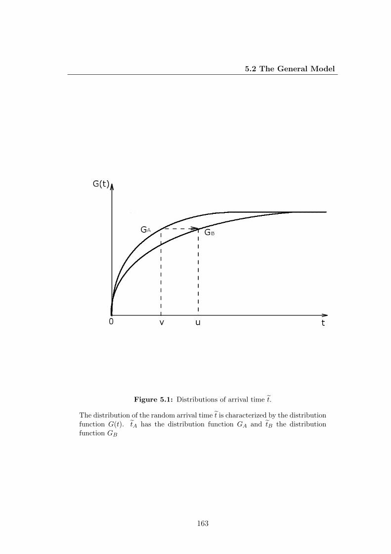
5.2 The General Model
Figure 5.1: Distributions of arrival time t.
The distribution of the random arrival time t is characterized by the distributionfunction G(t). tA has the distribution function GA and tB the distributionfunction GB
163

5.2 The General Model
That is, the expected utility of the market maker is kept constant throughout
transactions. Hereafter, we give the precise definition of S under the utility
indifference argument. Let w0 be the initial wealth of the market maker before a
purchase or a sell, and w be the change of his wealth during the course of waiting
to unwind the position (i.e. over the random waiting time t ).
Definition 4. The reservation price (spread) S, for the purchase or the sale of
one unit of the bond by the market maker, is defined as the solution of the equation
E[U(w0)] = E[U(w0 ± w + S)], (5.3)
where ± depends on whether the transaction is a purchase or a sell.
The reservation price S is essentially the spread at which the market maker is
indifferent (in the sense that his expected utility under competition is unchanged)
between doing nothing and receiving S now to have the position in his inventory.
Alternatively stated, S can be interpreted as the minimum amount that the mar-
ket maker wishes to receive to buy or sell one unit of the bond. Under Assumption
(G), the zero profit condition forces the market maker to post the spread S which
is exactly equal to the inventory holding cost in absence of information issues.
5.2.4 Brownian Motion and Poisson Arrivals
Now we will give an example of our general model, specified by a Brownian
Motion for asset prices and a homogeneous Poisson process for order arrivals.
Moreover, with some specific assumptions including the assumption about the
market maker’s utility function, the spread S can be quantified. We assume that
(K) The efficient price P of a bond under the ‘risk neutral’ measure moves as
an arithmetic Brownian Motion. That is, dP (s) = σ(s)dB(s), where B(s)
is a standard Brownian Motion. For expositional ease, σ(s) is assumed to
be time-invariant.
164

5.2 The General Model
(L) Except on the offering date 0, traders come to the market to buy or sell
one unit of the assets at a time. The arrivals of orders on a bond are
characterized by an independent homogeneous Poisson process, with the
arrival rate µ. Then, the random waiting time t follows an exponential
distribution with the expected waiting time 1/µ. The trading intensity
of each Type 1 trader is exogenously given and characterized by another
Poisson hazard rate, denoted by λ.
(M) The mean arrival rates from both sides (i.e. buying and selling) are approx-
imately equal so that the market is clear on average.1
Trading is performed via a monopolistic competitive market maker who stands
ready to trade. The market maker bridges the time gaps between the arrivals of
buyers and sellers to the market, and is compensated by charging the spread,
which is competitively set. Assumption (M) implies that the market maker is
seeking out the market spread that equilibrates buying and selling pressures.
Furthermore, we assume
(N) The risk-averse market maker has a negative exponential utility function,
i.e. U(w) = −e−γw, where γ is the absolute risk aversion of the market
maker and w is her wealth.
The negative exponential utility function combined with the above assump-
tions on asset prices and order arrivals enable us to calculate the spread analyti-
cally (as a function of the fundamental volatility and the order arrival rate).2
Proposition 1. The reservation price (spread) S for buying and selling one unit
of a bond is equal to γσ2
2µ, where γ is the absolute risk aversion of the market
maker, σ is the fundamental volatility, and µ is the arrival rate of orders on the
bond.
1From the perspective of the market maker, trading commences from the interim date 1.2Roger (1999) also derives the bid-ask spread in the utility indifference manner. However,
his derivation does not involve the order arrival rate or waiting time.
165

5.2 The General Model
Proof. By the definition of the reservation price S, Equation (5.3) can be written
as:
−e−γw0 = E[−e−γ(w0±w+S)|t], (5.4)
where w0 is the market maker’s initial wealth, t is the waiting time until the
offsetting order, and w is the change of the market maker’s wealth over the
waiting time t. Rearranging the terms in Equation (5.4) yield:
eγS = E[e±γw|t], (5.5)
Since under Assumption (K) and (N), w|t ∼ N(0, σ2t) and U(w) = −e−γw, we
have:
E[U(w)|t] = −eγ2σ2t/2, (5.6)
where ·|t means being conditional on t and E[·|t] is the conditional expectation.
Subsequently,
eγS = eγ2σ2t/2. (5.7)
Under Assumption (L) the expected waiting time is 1µ, thus the spread S is
obtained as:
S =γσ2
2µ. (5.8)
Hence, the spread increases while the price risk σ2 increases, and decreases
while the order arrival rate µ increases. As the market becomes more volatile,
the spread widens; as the orders arrive more frequently, the spread narrows. This
result is consistent with Stoll (1978a) and Bollen et al. (2004). Stoll (1978a) shows
that the relative bid-ask spread includes an inventory-holding-costs term which
equals the product of the return volatility and the expected time the market maker
166
5.2 The General Model
expects the position to be open. Bollen et al. (2004) show that the inventory
holding costs are positively related to the expected value of the square root of the
time between offsetting trades. If the market is perfectly liquid, that is µ→∞,
the spread vanishes (i.e. there is no transaction costs).
The expected waiting time is supposed to be far shorter than the maturity
of a bond. Intuitively, the market maker will not make a market for a bond, if
the waiting time of the offsetting order on this bond is too long. Alternatively
speaking, there is a probability that the market maker gets left with an inventory
of bonds on date 2. However, this probability is bound to be very small as the
expected waiting time of an offsetting order is much shorter than the maturity of
the bond. Moreover, the risk of getting left with an inventory is compensated by
charging bid-ask spreads. Therefore, we have
(O) A bond with the expected waiting time of orders 1/µ > C is considered to
be illiquid, where C is the cutoff value which is a constant. That is, if a
bond with the expected waiting time that is greater than C, the market
maker will choose not to make a market for this bond. The spread for an
illiquid bond is assumed to be 1 (that is S(µ) = 1, 1/µ > C, as in Figure
5.2.) .
In the next section we consider the decisions made by Type 1 traders. As we
will see later, the equilibrium is mostly determined by their actions.
5.2.5 The Investors’ Decisions
Recall that, on date 0 there are M Type 1 traders who make investment choices
out of a pool of N bonds. The total supply of the N bonds is K, with the supply
of Bond j ∈ N = 1, 2, . . . , N in terms of dollar value, denoted kj (that is,∑Nj=1 kj = K, 0 < kj).
Under Assumption (E) and (L), each Type 1 trader with an exogenously given
trading intensity is subject to the risk of liquidating some of her assets on date
1. More precisely, we assume that
167

5.2 The General Model
Figure 5.2: Spread
This figure shows that the spread is a function of the arrival rate:
S(µ) =
γσ2
2µ ,1µ < C,
1, 1µ ≥ C,
,
where µ is the order arrival rate, γ is the market maker’s absolute risk aversioncoefficient, σ is the volatility of the price dynamics of the bond, and C is thecutoff value which is a constant.
168
5.2 The General Model
(P) Each trader i ∈ M = 1, 2, . . . ,M with a trading intensity λi on date 0
purchases bonds with a total face value of Xi + Yi, where Xi is the total
tradable shares that she prepares for possible early liquidation on date 1
and Yi represents the total non-tradable shares that she will hold until
maturity (date 2). Let Xi = (Xi1, Xi2, ..., XiM) and Yi = (Yi1, Yi2, ..., YiM),
with Xi =∑
j∈NXij and Yi =∑
j∈N Yij, where Xij is the tradable shares of
bond j held by trader i, and Yij is the non-tradable shares of bond j held
by trader i.
Assumption (P) also implies that each trader i is essentially allocating her trading
intensity λi across the bonds.
Definition 5. An allocation of the trading intensity of trader i is defined as
hi = (hi1, hi2, ..., hiN), where hij the the normalized trading intensity of trader i
for bond j, with∑N
j=1 hij = 1 and hij ∈ [0, 1].
Therefore, the arrival rate of orders on bond j ∈ N can be expressed as
µj =∑i∈M
µij =∑i∈M
λihij, (5.9)
where µij is the arrival rate of orders on bond j from trader i. Moreover, we
assume that
(Q) The tradable shares Xij of bond j held by trader i is proportional to her
trading allocation. That is, Xij = hijXi.
Assumption (Q) basically means that, the more likely the trader will trade a
bond, the more tradable shares of the bond she holds.
Now we proceed to derive the initial bond price in the presence of illiquidity.
The introduction of transaction costs could change equilibrium prices. However,
it should be possible to identify equilibrium prices in a frictional cost economy as
being a function of the prices that prevail in a corresponding frictionless economy
plus some extra factor, and obviously the factor should depend upon the future
illiquidity of assets. Thus, price discounts or the extra yields are very likely to
169

5.2 The General Model
be associated with the future illiquidity of assets. In addition, equilibrium prices
may not be uniquely identifiable, but must preclude arbitrage opportunities.
In the presence of illiquidity or transaction costs, as previous stated, upon
purchasing a security a rational investor needs to take into account both the
likelihood and the potential costs of reselling the security back to the market at
a later point in time.
Let L ⊆ N and I ⊆ N represent the sets of liquid and illiquid bonds, respec-
tively. L⋃
I = N and L⋂
I = Φ, where Φ is the empty set. That is, a bond
must be either a liquid bond or an illiquid one, but not both at the same time.
On date 0, the price of a liquid bond P 0j , j ∈ L is determined as
P 0(µj) = 1− [1− e−µj ] · S(µj),1
µj< C, (5.10)
where µj = 1Mµj is the average arrival rate, and S(µj) is the spread, competitively
set by the market maker, which depends exclusively on µj.1
The price of a liquid bond in Equation 5.10 expressed as a discount of the
face value is derived using a risk-neutral pricing framework similar to the one
by Duffie & Singleton (1999) where the price of a defaultable bond is associated
with the default intensity as well as a factor which is related to liquidity effects
or carrying cost. Amihud & Mendelson (1986) and Vayanos & Vila (1999) show
that in order to induce the marginal investor to buy the asset, the price has to
fall by the present value of the transaction costs that he will incur.2 Therefore,
the discounted value which is the second term in Equation 5.10 is equal to the
probability of early liquidation (the term in the squared brackets) times the spread
charged by the market maker. The probability of early liquidation is a function of
the average arrival rate which could be interpreted as the trading intensity of the
marginal investors. The bond price P 0j is then equal to the marginal investors’
willingness to pay. In other words, risk-neutral investors are willing to pay a
1For expositional ease, we ignore the time value of interest or the risk-free interest rate asit is essentially the same across the bonds.
2In contrast, Vayanos (1998) shows that the PV term overstates the effect of transactioncosts on the risky stock price.
170
5.2 The General Model
premium on assets that help them when liquidity is needed.1
Since illiquid bonds are generally inferior to liquid ones, they should have
lower prices than those of liquid ones. Thus, we assume that:
(R) The price of the illiquid bond P 0j , j ∈ I is determined as
P 0(µj) = 1− γσ2
2M,
1
µj≥ C. (5.11)
The price of an illiquid bond in Equation 5.11 can be obtained by taking the
limit as µ approaches to zero in Equation 5.10. Therefore, bond prices across the
whole spectrum of liquid and illiquid bonds are expressed in terms of arrival rates
as shown in Figure 5.3.
With a subset of information, a reduced-form approach of modelling decision
making by pension funds or insurance companies is adopted. For Type 1 traders’
decisions on date 0, we assume that
(S) Each trader i ∈ M, with an endowment ei and a trading intensity λi solves
the following problem:
maxXi,Yi,hi
ei −∑j∈N
P 0j (hijXi + Yij), (5.12)
subject to:
1. total investment constraint:
Xi + Yi ≥ Fi, (5.13)
where Fi is the total face value required at maturity T .
2. pre-mature liquidation constraint:
∑j∈N
[1− S(µj)]hijXi ≥ Vi, (5.14)
1If we assume that traders are homogenous, in equilibrium every trader is essentially themarginal investor.
171
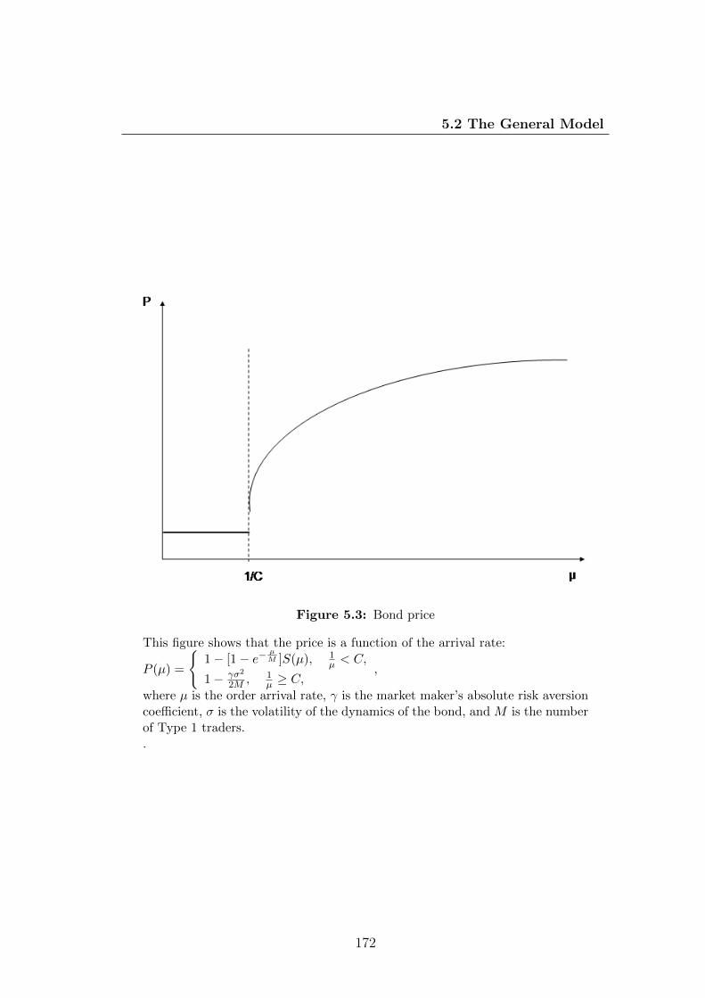
5.2 The General Model
Figure 5.3: Bond price
This figure shows that the price is a function of the arrival rate:
P (µ) =
1− [1− e−
µM ]S(µ), 1
µ < C,
1− γσ2
2M , 1µ ≥ C,
,
where µ is the order arrival rate, γ is the market maker’s absolute risk aversioncoefficient, σ is the volatility of the dynamics of the bond, and M is the numberof Type 1 traders..
172

5.2 The General Model
where Vi is the value required in the event of early liquidation,
3. market clearing constraints:
∑i∈M
hijXi + Yij = kj, j ∈ N, (5.15)
4. and nonnegativity constraints:
Xi ≥ 0, (5.16)
Yij ≥ 0, (5.17)
∑j∈N
hij = 1, 0 ≤ hij ≤ 1. (5.18)
The second term∑
j∈L P0j (hijXi + Yij) in the objective function (Equation
5.12) is the total investment, and thus, the objective function represents the post-
investment residual surplus, that is, the cash left over for trader i after making
her investment. In other words, the goal of each trader is to choose her portfolio
holding as well as her trading intensity allocation such that her residual surplus
is maximized.
The interpretation of the total investment constraint could be that pension
funds or insurance companies have long term liabilities which are hedged by
buying bonds. As being subject to the risk of pre-mature selling, a minimum
value in the event of early liquidation is required by each investor. It is the
minimum value that sellers expect to receive upon liquidation. This is similar
to the concept of the recovery value in the event of default in the credit risk
literature (e.g. Duffie & Singleton (1999)).
There are links between and restrictions on the values of the endowment ei,
the total face value Fi and the minimum value required upon liquidation Vi. ei
is greater than or equal to the (date 0) present value of Fi such that the investor
gets left with a non-negative surplus on the offering date. The sum of Fi is equal
173
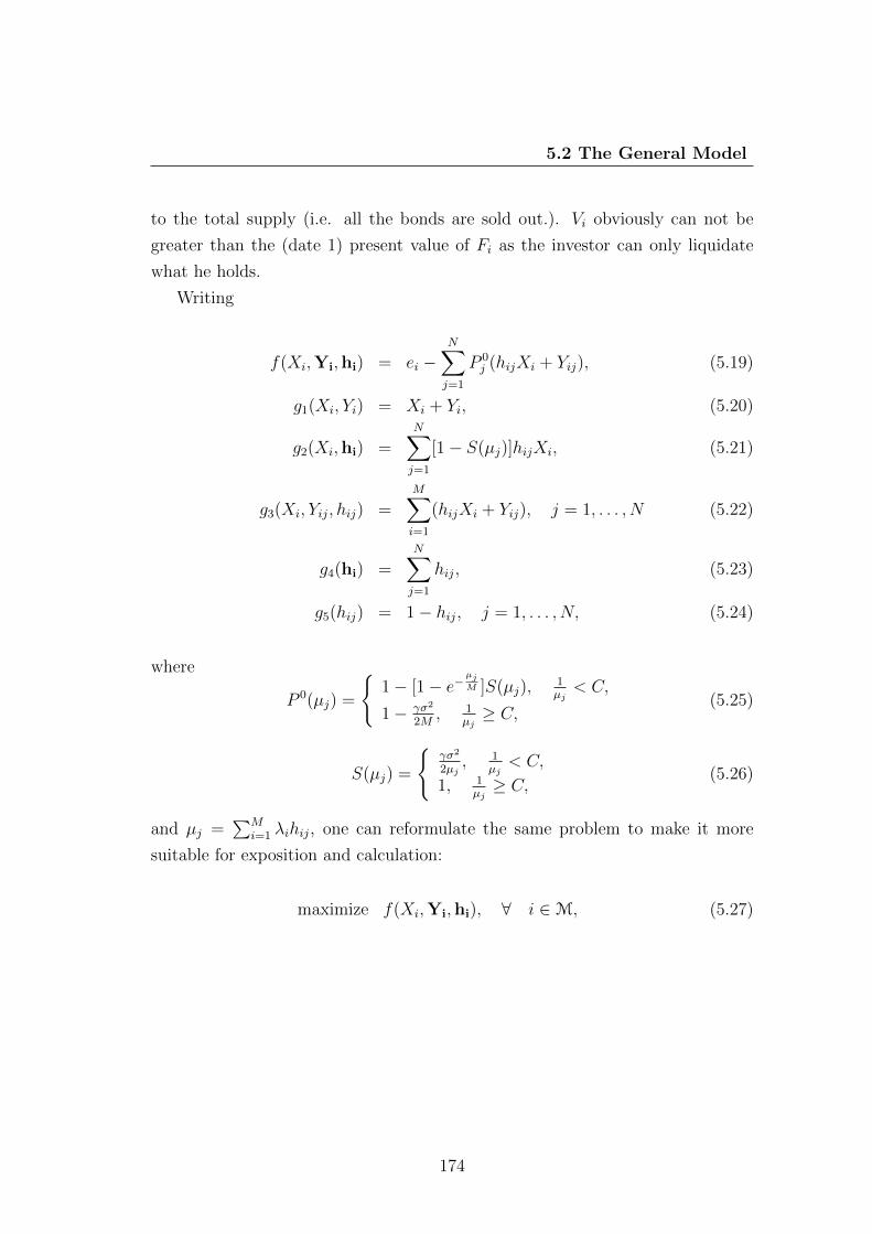
5.2 The General Model
to the total supply (i.e. all the bonds are sold out.). Vi obviously can not be
greater than the (date 1) present value of Fi as the investor can only liquidate
what he holds.
Writing
f(Xi,Yi,hi) = ei −N∑j=1
P 0j (hijXi + Yij), (5.19)
g1(Xi, Yi) = Xi + Yi, (5.20)
g2(Xi,hi) =N∑j=1
[1− S(µj)]hijXi, (5.21)
g3(Xi, Yij, hij) =M∑i=1
(hijXi + Yij), j = 1, . . . , N (5.22)
g4(hi) =N∑j=1
hij, (5.23)
g5(hij) = 1− hij, j = 1, . . . , N, (5.24)
where
P 0(µj) =
1− [1− e−
µjM ]S(µj),
1µj< C,
1− γσ2
2M, 1
µj≥ C,
(5.25)
S(µj) =
γσ2
2µj, 1
µj< C,
1, 1µj≥ C,
(5.26)
and µj =∑M
i=1 λihij, one can reformulate the same problem to make it more
suitable for exposition and calculation:
maximize f(Xi,Yi,hi), ∀ i ∈M, (5.27)
174

5.2 The General Model
subject to g1(Xi, Yi) ≥ Fi,g2(Xi,hi) ≥ Vi,g3(Xi, Yij, hij) = kj, j = 1, . . . , N,g4(hi) = 1,g5(hij) ≥ 0, j = 1, . . . , N,Xi ≥ 0,Yij ≥ 0, j = 1, . . . , N,hij ≥ 0, j = 1, . . . , N.
(5.28)
5.2.6 Time Line
For the economy defined above, we now summarize the sequence of events, agents’
actions, and the corresponding equilibria.
On date 0, each Type 1 trader given her endowment ei and trading intensity
λi maximizes her post-investment residual surplus by strategically choosing her
portfolio holding Xi,Yi and her trading intensity allocation hi, subject to
some external constraints (i.e. the total investment constraint Fi, pre-mature
liquidation constraint Vi, and market clearing constraints kj). The initial equilib-
rium is reached at the optimal portfolio holdings X∗i ,Y∗i , the optimal trading
intensity allocations h∗i , and the equilibrium bond prices P 0(µ∗j).
On date 1, Type 1 traders subject to early liquidation sell some of their
assets back to the marketplace. Since date 1 (but before date 2), Type 2 traders
randomly come to the market to buy bonds. The market maker stands ready to
bridge the gap between the sellers and the buyers by seeking the spreads which
equilibrate the market. Under Assumption (M), the subsequent equilibria are
reached at the market spreads S(µ∗j).
175
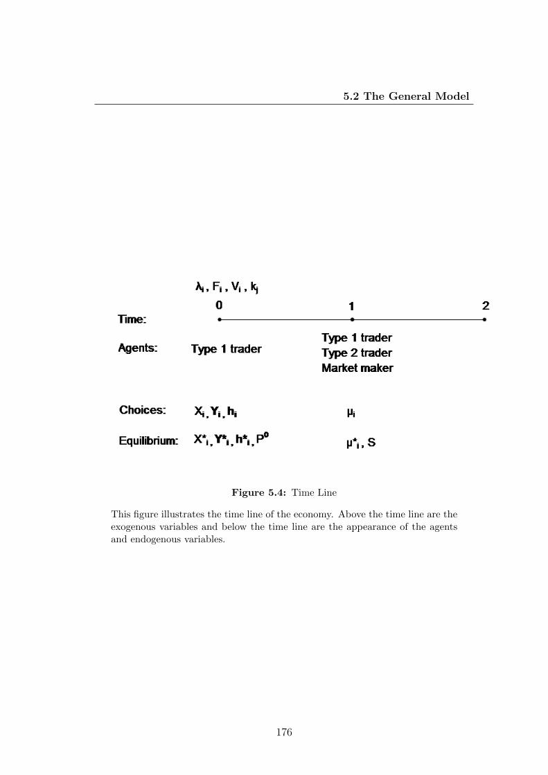
5.2 The General Model
Figure 5.4: Time Line
This figure illustrates the time line of the economy. Above the time line are theexogenous variables and below the time line are the appearance of the agentsand endogenous variables.
176
5.3 Characterization of Equilibrium
5.3 Characterization of Equilibrium
In this section, we describe how to obtain a characterization of the initial equilib-
rium. The objective of each investor i is to maximize the residual surplus given
in (5.27) by choosing her portfolio holding Xi,Yi, and her trading pattern hiand subject to some external constraints.
Now we can define the initial equilibrium:
Definition 6. An equilibrium (on date 0) consists of a collection of investors’
portfolio holdings X∗i ,Yi∗i∈M, trading patterns hi
∗i∈M, and a collection
of bond prices P 0(µ∗j)j∈N, such that the maximum in (5.27) is reached for all
i and the constraints in (5.28) are also satisfied.
The Lagrangian for the objective function in (5.27) that is to be maximized
is:
L(Xi,Yi,hi) = f(Xi,Yi,hi) + ν(g1(Xi, Yi)− Fi) + ω(g2(Xi,hi)− Vi) +N∑j=1
φjg5(hij)
−N∑j=1
ηj(g3(Xi, Yij, hij)− kj)− ξ(g4(hi)− 1)
+ εXi +N∑j=1
θjYij +N∑j=1
ϕjhij. (5.29)
Based on the above Lagrangian, the first order conditions implies that:
the equalities are
∂L
∂Xi
= 0 (5.30)
∂L
∂Yij= 0, j = 1, . . . , N, (5.31)
∂L
∂hij= 0, j = 1, . . . , N, (5.32)
177
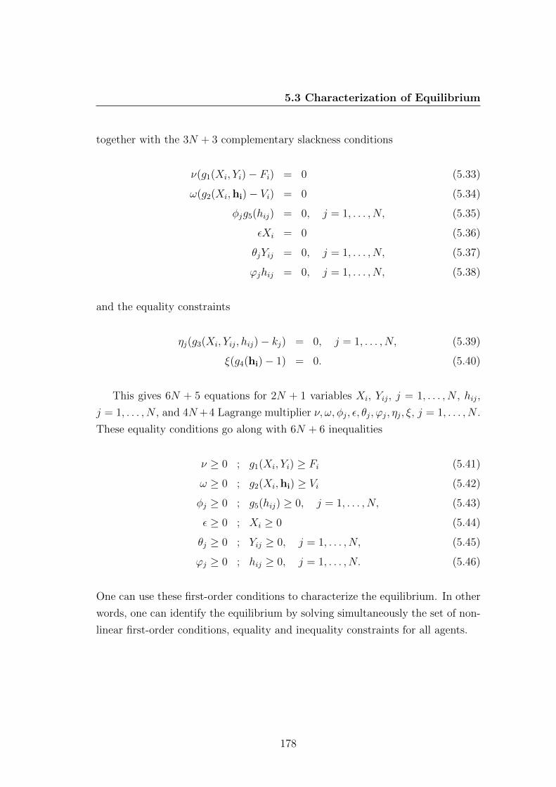
5.3 Characterization of Equilibrium
together with the 3N + 3 complementary slackness conditions
ν(g1(Xi, Yi)− Fi) = 0 (5.33)
ω(g2(Xi,hi)− Vi) = 0 (5.34)
φjg5(hij) = 0, j = 1, . . . , N, (5.35)
εXi = 0 (5.36)
θjYij = 0, j = 1, . . . , N, (5.37)
ϕjhij = 0, j = 1, . . . , N, (5.38)
and the equality constraints
ηj(g3(Xi, Yij, hij)− kj) = 0, j = 1, . . . , N, (5.39)
ξ(g4(hi)− 1) = 0. (5.40)
This gives 6N + 5 equations for 2N + 1 variables Xi, Yij, j = 1, . . . , N , hij,
j = 1, . . . , N , and 4N+4 Lagrange multiplier ν, ω, φj, ε, θj, ϕj, ηj, ξ, j = 1, . . . , N .
These equality conditions go along with 6N + 6 inequalities
ν ≥ 0 ; g1(Xi, Yi) ≥ Fi (5.41)
ω ≥ 0 ; g2(Xi,hi) ≥ Vi (5.42)
φj ≥ 0 ; g5(hij) ≥ 0, j = 1, . . . , N, (5.43)
ε ≥ 0 ; Xi ≥ 0 (5.44)
θj ≥ 0 ; Yij ≥ 0, j = 1, . . . , N, (5.45)
ϕj ≥ 0 ; hij ≥ 0, j = 1, . . . , N. (5.46)
One can use these first-order conditions to characterize the equilibrium. In other
words, one can identify the equilibrium by solving simultaneously the set of non-
linear first-order conditions, equality and inequality constraints for all agents.
178
5.4 Quantitative Implications
5.4 Quantitative Implications
To study the quantitative implications of our model, we consider the case where
the asset menu available to two homogeneous agents (e.g. with respect to the
constraints), who seek to maximize their residual surplus after the initial invest-
ments on date 0, consists of three bonds (e.g. bond 1, 2, and 3). In addition
to Assumption (A), (B) and (C), we assume that each of the three bonds are in
supply 100 dollars (i.e. k1 = k2 = k3 = $100).
Moreover, we use the following parameter values. We assume that on the
offering date 0 the investors, each with an endowment of 150 dollars (i.e. ei = 150,
i = 1, 2) and a trading intensity of 10 (i.e. λi = 10, i = 1, 2), seek to buy the
bonds to form their investment portfolios. For the total investment constraint,
we assume that each investor is required to realize a total face value of 150 dollars
at the maturity (i.e. Fi = 150, i = 1, 2). For the early liquidation constraint, we
vary the ratio of the minimum value required in the event of early liquidation to
the required total face value from 0 up to near 100 percent (i.e. ViFi∈ [0, 100%),
i = 1, 2). We will refer to it as the early liquidation ratio and for short the ratio
hereon.
We consider the setup where the competitive market maker has an exponential
utility with the absolute risk aversion coefficient γ = 1. The cutoff value C is
assumed to be equal to 1.1 This implies that the market maker is only willing to
make a market for a bond which they expect to be able to unwind before the bond
matures (i.e. the expected waiting time is less than 1 which is the time interval
between the interim date 1 and the maturity date 2.). For the price dynamics of
the bonds, we assume that the volatility σ is equal to 0.5.
5.4.1 Trading Behavior
We first consider the trading behaviors of the two agents in the equilibrium; one
can imagine this to be the case where each trader needs to allocate her trading
intensity among the three bonds.
1Altering the cutoff value will not change the results qualitatively.
179
5.4 Quantitative Implications
In Figure 5.5, we present the equilibrium allocations of the normalized trading
intensity of one of the agents. As we can see in Figure 5.5, when the early
liquidation ratio is below 33.10%, trading is concentrated almost on a single
bond whose trading intensity is 18. The trading intensities of both the other two
bonds are equal to 1 which is defined as the cutoff value of a bond being illiquid.
Correspondingly, Figure 5.6 shows that there exists only one tradable bond when
the ratio is below 33.10%.
When the quantity of bonds traded implies that there will be some tradable
and non-tradable bonds (e.g. the case described above), the identity of the ones
which are tradable could be the result of a ‘Sunspot’ equilibrium, where it is
optimal for traders to randomly label a subset of the bonds as the ‘liquid’ ones
and concentrate trading on them. A ‘Sunspot’ equilibrium is characterized as
a randomization over multiple certainty equilibria. In other words, the bonds
become liquid only because traders believe they will be liquid. It need not be
anything fundamental about the condition of those bonds. Anything that causes
them to anticipate a bond to be liquid will lead to concentration of trading in that
bond. A concentration of trading in liquid bonds results in liquidity externalities.
Bringing traders together creates liquidity externalities because the additional
traders arriving in the marketplace reduce trading costs for all traders.
There is extensive evidence that investors benefit from a liquidity externality
when they concentrate their trades in liquid assets. Amihud & Mendelson (1991)
compare the yields on short-term U.S. Treasury notes and bills both of which are
short-term single-payment instruments with the same maturities of 6 months or
less, generating the same cash flows and having identical risk. However, their
liquidity is different. Duffie (1996) mentions that it is common for traders to roll
a proportion of their positions into the successive current issues. Similar to our
argument, the tendency for reduced liquidity over time is to some extent a self-
fulfilling prophecy, since expecting lower liquidity will themselves lower liquidity.
Krishnamurthy (2002) find that variations in the off-the-run/on-the-run bond
spread are driven by aggregate factors related to investors’ preference for liquid
assets, although Goldreich et al. (2005) point out that the spread can also be
related to the expected future liquidity. Recently, Krishnamurthy & Vissing-
Jorgensen (2012) examine the spread between the interest rates customers receive
180

5.4 Quantitative Implications
on 6-month Federal Deposit Insurance Corporation (FDIC) insured certificates
of deposit (CDs) and 6-month Treasury bills, and find that the spread can only
be affected by liquidity.
Without loss of generality, when there is only one bond that is traded, bond
1 is labeled as the liquid one. Subsequently, when only two bonds are tradable,
bond 1 and 2 are labeled as the liquid ones. While the ratio increases from 33.10%
up to 65.79%, the normalized trading intensity of bond 1 decreases from 0.9 to
0.475, and the normalized trading intensity of bond 2 increases from 0.05 to 0.475.
At the same time the normalized trading intensity of bond 3 remains unchanged
at 0.05. Figure 5.6 shows that the number of tradable bonds becomes two when
the ratio is in between 33.10% and 65.79%.
As the ratio goes beyond 65.79%, the normalized trading intensities for both
bond 1 and 2 decrease from 0.475 to 1/3, whereas the normalized trading intensity
of bond 3 increases from 0.05 to 1/3. That means that, with µ1 = µ2 = µ3 = 20/3,
investors can achieve the highest early liquidation ratio. As shown in Figure 5.6,
all the three bonds are tradable or liquid when the ratio is above 65.79%.
In summary, for low early liquidation ratios, investors have strong preference
for concentrating trading on a small number of bonds. While the ratio increases,
investors start to spread trading over more bonds. Figure 5.6 shows that as the
ratio increases, the number of tradable bonds increases stepwise. Furthermore,
Figure 5.7 indicates that by concentrating trading on a limited number of bonds
investors could gain more surplus, whereas spreading trading over more issues
reduces their residual surplus and achieves higher liquidation ratio. The distance
between the blue solid line and the black dashed line is essentially the extra
surplus that investors gain by concentrating liquidity. The result is partially
consistent with Economides & Siow (1988) who show that liquidity consideration
will limit the number of markets in a competitive economy. Investors may prefer
fewer markets so that liquidity is enhanced in those markets, even though they
will have fewer assets to choose from.
181
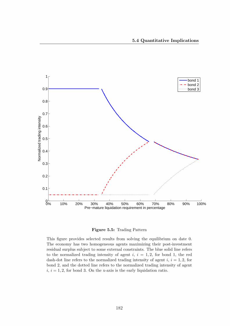
5.4 Quantitative Implications
Pre−mature liquidation requirement in percentage
Nor
mal
ized
trad
ing
inte
nsity
0% 10% 20% 30% 40% 50% 60% 70% 80% 90% 100%0
0.1
0.2
0.3
0.4
0.5
0.6
0.7
0.8
0.9
1bond 1bond 2bond 3
Figure 5.5: Trading Pattern
This figure provides selected results from solving the equilibrium on date 0.The economy has two homogeneous agents maximizing their post-investmentresidual surplus subject to some external constraints. The blue solid line refersto the normalized trading intensity of agent i, i = 1, 2, for bond 1, the reddash-dot line refers to the normalized trading intensity of agent i, i = 1, 2, forbond 2, and the dotted line refers to the normalized trading intensity of agenti, i = 1, 2, for bond 3. On the x-axis is the early liquidation ratio.
182
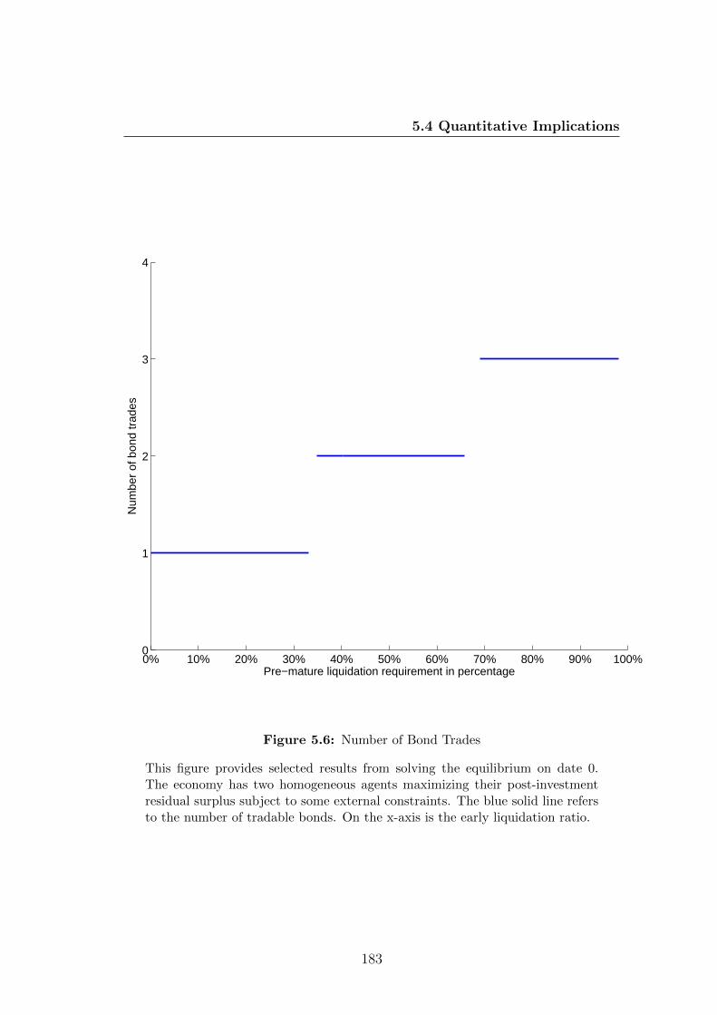
5.4 Quantitative Implications
0% 10% 20% 30% 40% 50% 60% 70% 80% 90% 100%0
1
2
3
4
Pre−mature liquidation requirement in percentage
Num
ber
of b
ond
trad
es
Figure 5.6: Number of Bond Trades
This figure provides selected results from solving the equilibrium on date 0.The economy has two homogeneous agents maximizing their post-investmentresidual surplus subject to some external constraints. The blue solid line refersto the number of tradable bonds. On the x-axis is the early liquidation ratio.
183
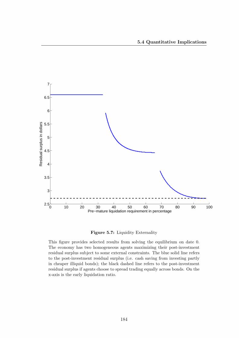
5.4 Quantitative Implications
0 10 20 30 40 50 60 70 80 90 1002.5
3
3.5
4
4.5
5
5.5
6
6.5
7
Pre−mature liquidation requirement in percentage
Res
idua
l sur
plus
in d
olla
rs
Figure 5.7: Liquidity Externality
This figure provides selected results from solving the equilibrium on date 0.The economy has two homogeneous agents maximizing their post-investmentresidual surplus subject to some external constraints. The blue solid line refersto the post-investment residual surplus (i.e. cash saving from investing partlyin cheaper illiquid bonds); the black dashed line refers to the post-investmentresidual surplus if agents choose to spread trading equally across bonds. On thex-axis is the early liquidation ratio.
184
5.4 Quantitative Implications
5.4.2 Portfolio Holdings
In Figure 5.8, we present the tradable shares held by one of the agents. As the
early liquidation ratio starts to increase, the tradable shares of bond 1 increase
sharply, whereas a very large proportion of the other two bonds remains illiquid.1
When the ratio passes 33.10%, the non-tradable shares of bond 1 decrease to
zero. Meanwhile more tradable shares are being supplied by bond 2. In the end,
investors need to keep all their portfolio holdings tradable in order to fulfill the
early liquidation constraint. For instance, in the top panel of Figure 5.9, when the
ratio is equal to 33.10%, investors are better off by keeping only bond 1 tradable
and locking away the other two bonds. Then, in the middle panel where the ratio
is increased to 65.79%, in order to fulfill a higher early liquidation constraint, all
the shares of bond 1 and 2 need to be tradable. Finally, in the bottom panel
investors need to have all their holdings of bond 1, 2 and 3 tradable so that
they can achieve an even tougher constraint, which means that they anticipate
to unwind all their holdings prior to maturity.
In summary, the aggravate tradable (non-tradable) shares increase (decrease)
as the early liquidation ratio increases. Intuitively, for low early liquidation ratios,
investors have a certain degree of freedom to fill a large part of their investment
portfolios with cheap and illiquid bonds. For high early liquidation ratios, in
order to avoid high transaction costs investors need to prepare themselves with
more liquid bonds. Therefore, our model predicts that economic conditions, or
funding conditions of investors or firms may affect liquidity demands. The equi-
librium results from the behaviors of the forward looking investors who increase
demand for liquid assets ahead of economic downturns. This is partially con-
sistent with Holmstrom & Tirole (2001) show that leverage ratios and capital
adequacy requirements affect the corporate demand for liquid assets.
5.4.3 Bond Prices
In Figure 5.10, we present the equilibrium bond prices on date 0. As we know from
the model, the bond prices are exclusively determined by the trading intensities
1The resulting tradable shares correspond to the equilibrium with equality pre-mature liq-uidation constraint.
185
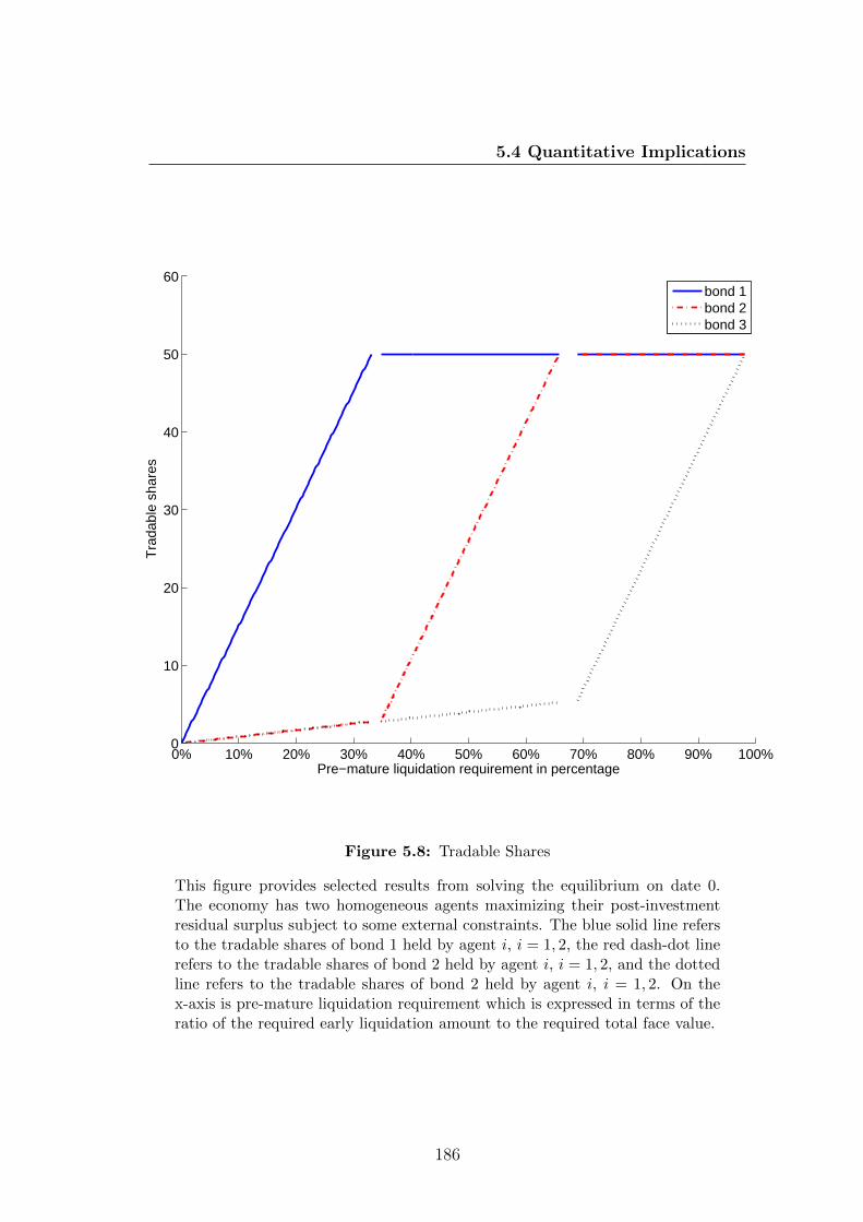
5.4 Quantitative Implications
0% 10% 20% 30% 40% 50% 60% 70% 80% 90% 100%0
10
20
30
40
50
60
Pre−mature liquidation requirement in percentage
Tra
dabl
e sh
ares
bond 1bond 2bond 3
Figure 5.8: Tradable Shares
This figure provides selected results from solving the equilibrium on date 0.The economy has two homogeneous agents maximizing their post-investmentresidual surplus subject to some external constraints. The blue solid line refersto the tradable shares of bond 1 held by agent i, i = 1, 2, the red dash-dot linerefers to the tradable shares of bond 2 held by agent i, i = 1, 2, and the dottedline refers to the tradable shares of bond 2 held by agent i, i = 1, 2. On thex-axis is pre-mature liquidation requirement which is expressed in terms of theratio of the required early liquidation amount to the required total face value.
186
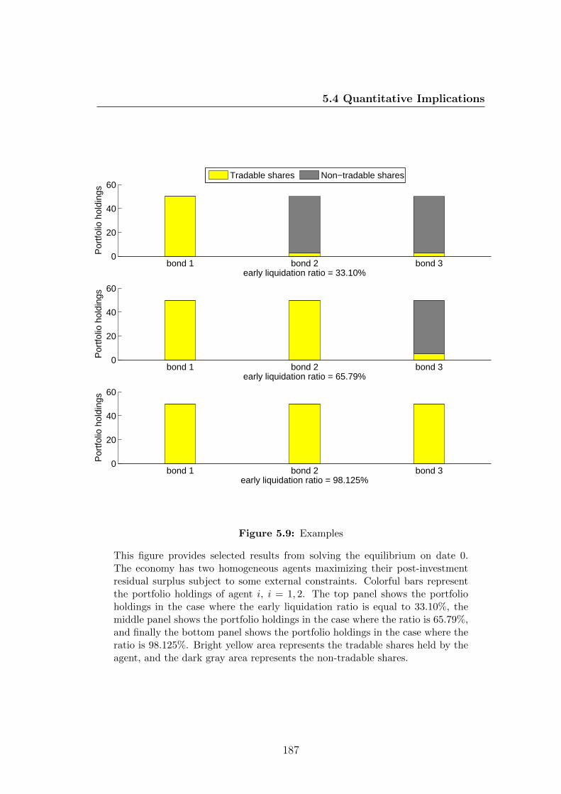
5.4 Quantitative Implications
bond 1 bond 2 bond 30
20
40
60
Por
tfolio
hol
ding
s
early liquidation ratio = 33.10%
bond 1 bond 2 bond 30
20
40
60
Por
tfolio
hol
ding
s
early liquidation ratio = 65.79%
bond 1 bond 2 bond 30
20
40
60
Por
tfolio
hol
ding
s
early liquidation ratio = 98.125%
Tradable shares Non−tradable shares
Figure 5.9: Examples
This figure provides selected results from solving the equilibrium on date 0.The economy has two homogeneous agents maximizing their post-investmentresidual surplus subject to some external constraints. Colorful bars representthe portfolio holdings of agent i, i = 1, 2. The top panel shows the portfolioholdings in the case where the early liquidation ratio is equal to 33.10%, themiddle panel shows the portfolio holdings in the case where the ratio is 65.79%,and finally the bottom panel shows the portfolio holdings in the case where theratio is 98.125%. Bright yellow area represents the tradable shares held by theagent, and the dark gray area represents the non-tradable shares.
187
5.4 Quantitative Implications
or the arrival rates of the bonds. When the early liquidation ratio is below
33.10%, the equilibrium price of bond 1 is much higher that those of the other
two bonds. As the ratio increases from 33.10% to 65.79%, the price of bond 2
increases steeply, while the price of bond 1 decreases very slowly. When the ratio
goes beyond 65.79%, the prices of the three bonds finally converge.
The feature, that bond prices increase faster than that they decrease, is the
ultimate reason that investors have strong preference for concentrating trading.
As investors spread trading over more bonds, the surplus they lose from making
more bonds tradable is much higher than the surplus gained by reducing the
prices of the perviously liquid bonds. Therefore, investors have an incentive to
concentrate trading, subject to economic or funding conditions.
In addition, one could imagine that agents with high early liquidation ratios
are short-term investors, and agents with low early liquidation ratios are long-
term investors. Long-term investors prefer high-yield illiquid bonds to low-yield
liquid ones, whereas short-term investors having in mind future transaction costs
would like to have more liquid bonds in their portfolios. This clientele effect is
well-documented in the literature (See Amihud & Mendelson (1986), Vayanos &
Vila (1999), and Vayanos & Wang (2007)).
188

5.4 Quantitative Implications
0% 10% 20% 30% 40% 50% 60% 70% 80% 90% 100%0.93
0.94
0.95
0.96
0.97
0.98
0.99
1
Pre−mature liquidation requirement in percentage
Equ
ilibr
ium
bon
d pr
ice
bond 1bond 2bond 3
Figure 5.10: Equilibrium Bond Price
This figure provides selected results from solving the equilibrium on date 0.The economy has two homogeneous agents maximizing their post-investmentresidual surplus subject to some external constraints. The blue solid line refersto the equilibrium price of bond 1, the red dash-dot line refers to the equilibriumprice of bond 2, and the dotted line refers to the equilibrium price of bond 3.On the x-axis is pre-mature liquidation requirement which is expressed in termsof the ratio of the required early liquidation amount to the required total facevalue.
189

5.5 Summary and Conclusion
5.5 Summary and Conclusion
Theoretical studies normally impose ex ante assumptions on asset liquidity. Our
study takes a step forward in bridging such a gap by developing an equilibrium
model in which trading concentration is created endogenously.
We show that (otherwise identical) bonds may differ in liquidity. Investors
have strong preference for trading concentration, subject to liquidity constraints.
We also show that the identity of which bonds do trade could be a result of
a ‘Sunspot’ equilibrium. Changing liquidity constraints can lead to different
equilibrium configurations where trading is spread over bonds. By capitalizing
the concepts of stochastic dominance and utility indifference price, and some
specific assumptions including the assumptions on the asset value and the order
arrival rate, the equilibrium prices and bid-ask spreads can be quantified.
190

Chapter 6
Further Research
There are potentially a few directions towards which we can further our current
studies. We will briefly discuss them in this section.
6.1 Higher Frequency and More Bonds
In our current study we analyze the corporate bond liquidity at a daily frequency,
it would be interesting to look at how liquidity and liquidity premium behave at
a higher frequency level, for instance, at a trade-by-trade frequency.
Moreover, one of the main limits of our extended Roll model is that the
variance of the nonpreservable efficient price is time-invariant. In the literature of
estimating realized variance, Bandi & Russell (2006) use sample moments of high
frequency returns to identify both the time-varying variance of the unobservable
efficient returns and the variance of the microstructure noise which in our model is
referred as the half spread. Hansen & Lunde (2006) study the implications of the
market microstructure noise in high-frequency data for the realized variance under
a general specification for the noise. Bandi & Russell (2008) derive a MSE optimal
high-frequency sampling theory to reduce the microstructure noise-induced bias.
Although the focus of these papers is on the realized variance, combining the time-
varying component and high frequency data with a more realistic microstructure
component (e.g. discreteness, different type of trades, and correlation between
191

6.2 Heterogenous agents
the underlying price process and the microstructure noise) will be producing a
cleaner estimation of the bid-ask spread.
Our empirical study only focuses on bonds issued by a specific company.
Blanco et al. (2005) use daily mid-market quotes of CDS and daily interpolated
bond yields on 33 reference entities to study the empirical relation between CDSs
and credit spreads. The sample used by Longstaff et al. (2005) consists of CDS
premia for 5-year contracts and corporate bond prices for 68 firms (Aaa through
BB). Bao et al. (2011) estimate their illiquidity measure by using either trade-by-
trade prices or end of the day prices of 1032 bonds (Aaa through C). Although
the availability and accuracy of high frequency transaction data of both CDSs
and corporate bonds significantly reduce the potential dataset, it is still possible
to apply our methodology to a larger sample set by including bonds with different
ratings or bonds issued by firms in different countries or industries. With a larger
set of data, we will be able to examine liquidity both at the market level and
at the individual bond level. We can analyse liquidity variations across rating
categories and sectors.
6.2 Heterogenous agents
In our third study, we analyze bond liquidity in an equilibrium economy with
multiple agents who are homogeneous (i.e. with respect to liquidity constraints).
Other studies also consider agents who are heterogeneous with respect to en-
dowments or preference. These include Bhamra & Uppal (2010) and Buss et al.
(2011) where agents have time-additive preferences or a recursive utility. In our
risk neutral approach, to allow agents with heterogeneous liquidity constraints,
which could lead to the case where agents with different trading allocations, might
be more challenging than the homogeneous case which is already complicated
enough.
192
Chapter 7
Conclusions
In this thesis we study liquidity in bond markets from both the empirical and
theoretical point of view. In the following, we recapitulate the key findings and
conclusions of our research.
7.1 Summary of Major Findings
7.1.1 An Extended Model of Estimating Effective Bid-ask
Spread
In this study we present an extended model for the estimation of the effective
bid-ask spread that allows trades to execute either inside or outside the quoted
bid-ask spread. We extend the Roll model by adding an extra parameter λ, the
so-called ‘spread multiplier’, which is constructed to separate spreads of different
magnitudes. In other words, we generalize Roll’s spread estimator (a scalar) to
include a vector of spreads with associated probabilities.
The extended model is estimated by a Bayesian Gibbs approach based on
only transaction data. Since we treat the models with different values of λ as
competitive models, the value of λ is determined via a Bayesian model selection
method by comparing marginal likelihoods evaluated from the Gibbs outputs.
The new model together with the model estimation and selection procedures
offers an alternative way to more accurately estimate the effective bid-ask spread
193
7.1 Summary of Major Findings
and the underlying return variance.
7.1.2 Non-default Yields Spreads and Illiquidity of Cor-
porate Bonds
In this study, we use the data from both credit default swap and corporate bond
markets to study the relationships between different liquidity proxies and the non-
default component of corporate bond spreads as well as our illiquidity measure.
Firstly, we separate the non-default component of bond spreads from the
default one by applying a non-parametric reduced-form credit risk model to si-
multaneously price credit default swaps and corporate bonds.
We then apply a Kalman filter extension of the original Roll model to estimate
the unobservable non-default bond residuals as well as our illiquidity measure.
By using the panel data during 2006 - 2010, we examine the relationships
between different liquidity proxies and the non-default component of corporate
bond yield spreads as well as the illiquidity measure via panel regressions. The
empirical results that the illiquidity measure is related to both the bond charac-
teristics and the liquidity proxies based on the transaction-level data, therefore
reflecting the current level of market liquidity. We also find that the non-default
component of the yield spreads has a nonlinear and positive relationship with the
time-to-maturity and a positive relationship with the illiquidity measure as well
as the default risk, therefore reflecting the future expected liquidity.
7.1.3 An Equilibrium Model of Liquidity in Bond Markets
This study provides an alternative theory of liquidity, exclusively based on inven-
tory holding risk, to understand why there exist heterogenous levels of liquidity
among otherwise identical bonds.
We develop an equilibrium model in which the identity of which bonds are
liquid, and how large their spreads and liquidity discounts (or liquidity premium)
are, are determined endogenously. We assume that in the economy a number
of (otherwise identical) bonds are exchanged among the market participants: a
194

7.1 Summary of Major Findings
set of risk neutral investors with exogenously determined cash flow and liquidity
constraints form their investment portfolios by maximizing their post-investment
residual surplus on the offering date; another set of risk neutral traders come
later on to buy these bonds; a risk averse competitive market maker acts as the
whole financial intermediaries by bridging the gaps between buyers and sellers
and charges spreads for bearing the inventory-holding risk.
By utilizing the concepts of stochastic dominance, utility indifference pricing
and the assumptions on the dynamics of bond prices and the order arrival rate,
the equilibrium bond prices and bid-ask spreads can be quantified.
Investors have strong preference for trading concentration, subject to liquidity
constraints. In particular, when the quantity of bonds which do trade implies
that there will be some tradable and non-tradable bonds, the identity of the
ones which do trade could be the result of a ‘Sunspot’ equilibrium. Traders with
tougher liquidity constraints need to spread trading over more bonds and have
more tradable shares in their portfolios. Therefore, asset holdings and trading
patterns are sensitive to liquidity constraints.
195
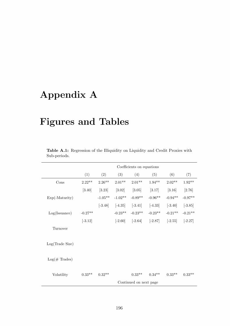
Appendix A
Figures and Tables
Table A.1: Regression of the Illiquidity on Liquidity and Credit Proxies withSub-periods.
Coefficients on equations
(1) (2) (3) (4) (5) (6) (7)
Cons 2.22** 2.26** 2.01** 2.01** 1.94** 2.02** 1.92**
[3.40] [3.23] [3.02] [3.05] [3.17] [3.16] [2.76]
Exp(-Maturity) -1.05** -1.02** -0.89** -0.96** -0.94** -0.97**
[-3.48] [-4.35] [-3.41] [-4.33] [-3.40] [-3.85]
Log(Issuance) -0.27** -0.23** -0.23** -0.23** -0.21** -0.21**
[-3.12] [-2.60] [-2.64] [-2.87] [-2.55] [-2.27]
Turnover
Log(Trade Size)
Log(# Trades)
Volatility 0.33** 0.32** 0.33** 0.34** 0.33** 0.33**
Continued on next page
196
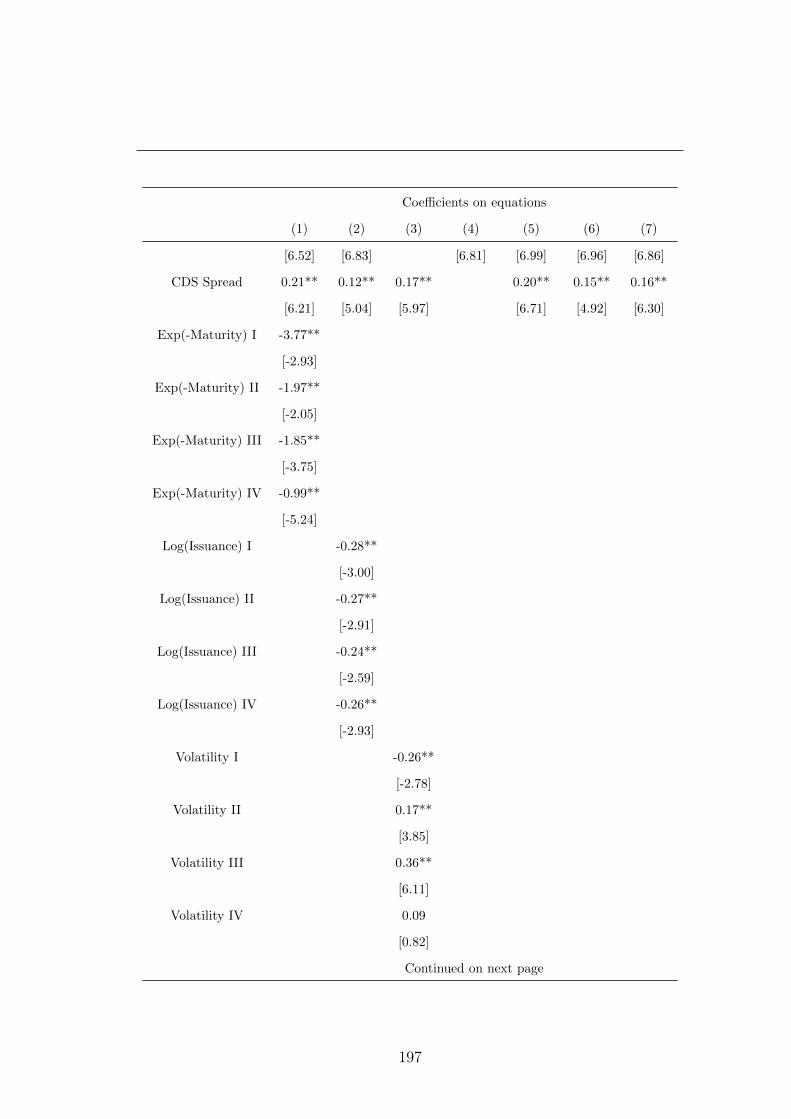
Coefficients on equations
(1) (2) (3) (4) (5) (6) (7)
[6.52] [6.83] [6.81] [6.99] [6.96] [6.86]
CDS Spread 0.21** 0.12** 0.17** 0.20** 0.15** 0.16**
[6.21] [5.04] [5.97] [6.71] [4.92] [6.30]
Exp(-Maturity) I -3.77**
[-2.93]
Exp(-Maturity) II -1.97**
[-2.05]
Exp(-Maturity) III -1.85**
[-3.75]
Exp(-Maturity) IV -0.99**
[-5.24]
Log(Issuance) I -0.28**
[-3.00]
Log(Issuance) II -0.27**
[-2.91]
Log(Issuance) III -0.24**
[-2.59]
Log(Issuance) IV -0.26**
[-2.93]
Volatility I -0.26**
[-2.78]
Volatility II 0.17**
[3.85]
Volatility III 0.36**
[6.11]
Volatility IV 0.09
[0.82]
Continued on next page
197
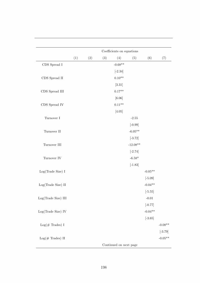
Coefficients on equations
(1) (2) (3) (4) (5) (6) (7)
CDS Spread I -0.68**
[-2.34]
CDS Spread II 0.10**
[3.31]
CDS Spread III 0.17**
[6.06]
CDS Spread IV 0.11**
[4.05]
Turnover I -2.55
[-0.99]
Turnover II -6.05**
[-3.72]
Turnover III -12.08**
[-2.74]
Turnover IV -6.58*
[-1.83]
Log(Trade Size) I -0.05**
[-5.09]
Log(Trade Size) II -0.04**
[-5.55]
Log(Trade Size) III -0.01
[-0.77]
Log(Trade Size) IV -0.04**
[-3.65]
Log(# Trades) I -0.08**
[-3.79]
Log(# Trades) II -0.05**
Continued on next page
198

Coefficients on equations
(1) (2) (3) (4) (5) (6) (7)
[-4.16]
Log(# Trades) III -0.01
[-0.58]
Log(# Trades) IV -0.05**
[-2.04]
Obs 10196 10196 10196 10196 10183 10184 10195
R2 20.36% 21.01% 20.87% 20.85% 21.07% 21.52% 20.68%
199
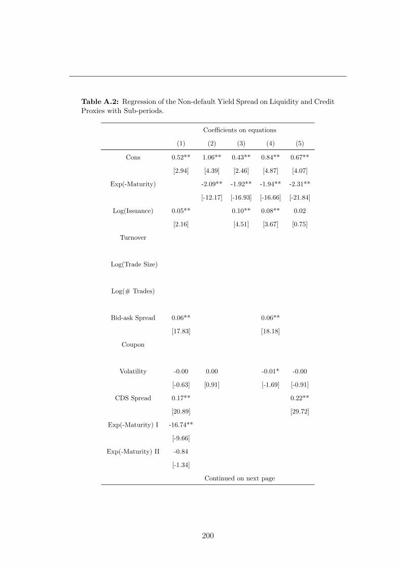
Table A.2: Regression of the Non-default Yield Spread on Liquidity and CreditProxies with Sub-periods.
Coefficients on equations
(1) (2) (3) (4) (5)
Cons 0.52** 1.06** 0.43** 0.84** 0.67**
[2.94] [4.39] [2.46] [4.87] [4.07]
Exp(-Maturity) -2.09** -1.92** -1.94** -2.31**
[-12.17] [-16.93] [-16.66] [-21.84]
Log(Issuance) 0.05** 0.10** 0.08** 0.02
[2.16] [4.51] [3.67] [0.75]
Turnover
Log(Trade Size)
Log(# Trades)
Bid-ask Spread 0.06** 0.06**
[17.83] [18.18]
Coupon
Volatility -0.00 0.00 -0.01* -0.00
[-0.63] [0.91] [-1.69] [-0.91]
CDS Spread 0.17** 0.22**
[20.89] [29.72]
Exp(-Maturity) I -16.74**
[-9.66]
Exp(-Maturity) II -0.84
[-1.34]
Continued on next page
200
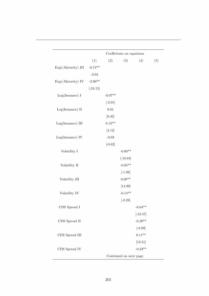
Coefficients on equations
(1) (2) (3) (4) (5)
Exp(-Maturity) III -0.74**
-3.04
Exp(-Maturity) IV -2.90**
[-24.15]
Log(Issuance) I -0.07**
[-2.01]
Log(Issuance) II 0.01
[0.42]
Log(Issuance) III 0.13**
[4.12]
Log(Issuance) IV -0.03
[-0.82]
Volatility I -0.60**
[-10.84]
Volatility II -0.05**
[-1.98]
Volatility III 0.08**
[14.99]
Volatility IV -0.14**
[-8.28]
CDS Spread I -6.64**
[-24.57]
CDS Spread II -0.29**
[-8.89]
CDS Spread III 0.11**
[13.51]
CDS Spread IV -0.33**
Continued on next page
201
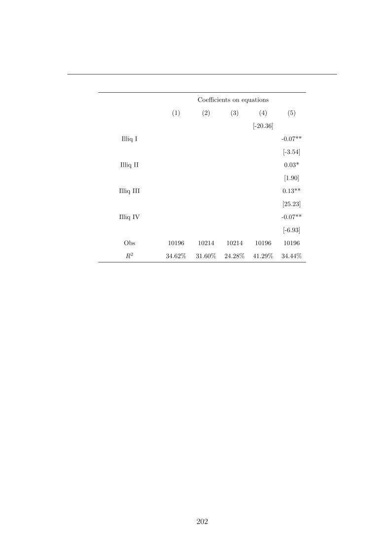
Coefficients on equations
(1) (2) (3) (4) (5)
[-20.36]
Illiq I -0.07**
[-3.54]
Illiq II 0.03*
[1.90]
Illiq III 0.13**
[25.23]
Illiq IV -0.07**
[-6.93]
Obs 10196 10214 10214 10196 10196
R2 34.62% 31.60% 24.28% 41.29% 34.44%
202
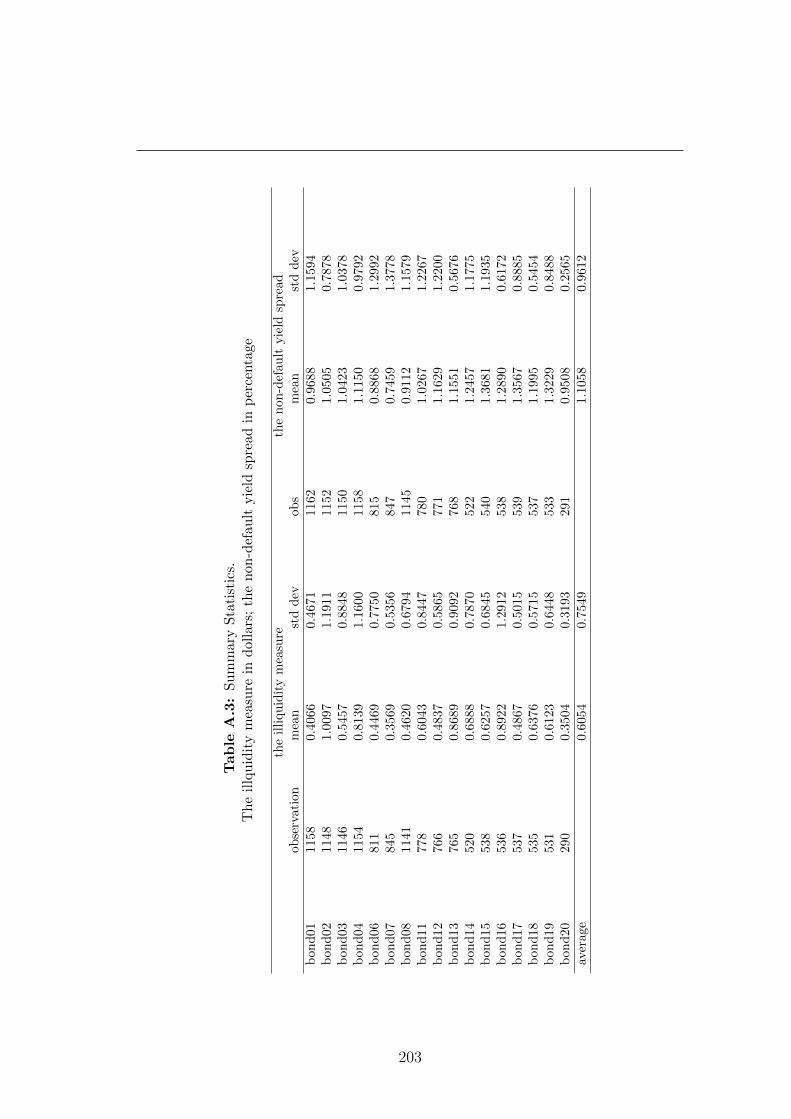
Table
A.3:
Su
mm
ary
Sta
tist
ics.
Th
eil
lqu
idit
ym
easu
rein
dol
lars
;th
en
on-d
efau
ltyie
ldsp
read
inp
erce
nta
ge
the
illi
qu
idit
ym
easu
reth
enon
-def
au
ltyie
ldsp
read
obse
rvat
ion
mea
nst
dd
evob
sm
ean
std
dev
bon
d01
1158
0.40
660.4
671
1162
0.9
688
1.1
594
bon
d02
1148
1.00
971.1
911
1152
1.0
505
0.7
878
bon
d03
1146
0.54
570.8
848
1150
1.0
423
1.0
378
bon
d04
1154
0.81
391.1
600
1158
1.1
150
0.9
792
bon
d06
811
0.44
690.7
750
815
0.8
868
1.2
992
bon
d07
845
0.35
690.5
356
847
0.7
459
1.3
778
bon
d08
1141
0.46
200.6
794
1145
0.9
112
1.1
579
bon
d11
778
0.60
430.8
447
780
1.0
267
1.2
267
bon
d12
766
0.48
370.5
865
771
1.1
629
1.2
200
bon
d13
765
0.86
890.9
092
768
1.1
551
0.5
676
bon
d14
520
0.68
880.7
870
522
1.2
457
1.1
775
bon
d15
538
0.62
570.6
845
540
1.3
681
1.1
935
bon
d16
536
0.89
221.2
912
538
1.2
890
0.6
172
bon
d17
537
0.48
670.5
015
539
1.3
567
0.8
885
bon
d18
535
0.63
760.5
715
537
1.1
995
0.5
454
bon
d19
531
0.61
230.6
448
533
1.3
229
0.8
488
bon
d20
290
0.35
040.3
193
291
0.9
508
0.2
565
aver
age
0.60
540.7
549
1.1
058
0.9
612
203
Appendix B
Useful Information
B.1 Stochastic Dominance
Stochastic dominance provides a rather general framework in which to model
the market maker’s decisions. It will also be sufficient for our purposes. Before
applying it we will briefly summarize the key results that we will need.
In comparing two prospects, stochastic dominance measures to what extent ei-
ther has higher probabilities associated with higher payoffs and lower probabilities
associated with lower payoffs. Any rational investor (who is an expected utility
maximizer) would prefer prospect A over prospect B if both have the same possi-
ble payoffs, but A has higher probabilities associated with higher-valued payoffs
and lower probabilities associated with lower-valued payoffs.
First-order stochastic dominance (FSD), originally developed by Quirk &
Saposnik (1962), attempts to order uncertain prospects assuming only that in-
vestors’ utility functions are monotonically increasing with respect to wealth.
Specifically, prospect A first-order stochastically dominates Prospect B, if and
only if there exist some ξ such that XBd=XA + ξ where ξ is a non-positive ran-
dom variable1. In other words, investors prefer A to B, regardless of their risk
1 d= means “is equivalent in distribution to”.
204

B.2 Mean-Preserving Spreads
preferences, as long as their utility function is monotonically increasing, i.e., more
wealth is preferred to less.
Second-order stochastic dominance (SSD) assumes, in addition to monotonic
utility functions, weak global risk aversion (i.e., diminishing marginal utility for
wealth). SSD was developed by Hadar & Russell (1969). In terms of distribution
functions FA and FB, prospect A is second-order stochastically dominant over
prospect B if and only if∫ x−∞[FB(t)−FA(t)]dt ≥ 0 for all x, with strict inequality
for some x. In other words, risk-averse investors (who are expected utility maxi-
mizers with monotonically increasing and concave utility function) prefer A to B
if and only if the above integral condition holds on their distribution functions.
B.2 Mean-Preserving Spreads
A mean-preserving spread (MPS) is a change from one probability distribution
FA to another probability distribution FB, where FB is formed by spreading out
one or more portions of FA’s probability density function while leaving the mean
unchanged. As such, the concept of mean-preserving spreads provides a stochastic
ordering of equal-mean probability distributions. SSD is closely related to mean-
preserving spread through Rothschild and Stiglitz Theorem.
Prospect A second-order stochastically dominates prospect B, if and only if
there exist some ξ and ε such that XBd=XA + ξ + ε, with ξ ≤ 0, and with
E(ε|XA + ξ) = 0 for all values of XA + ξ (ε is a fair game with respect to XA + ξ).
Therefore, by the Rothschild and Stiglitz Theorem (Rothschild (1970)), if A
and B have the same mean (so that the random variable ξ degenerates to the
fixed number 0), then B is second-order stochastically dominated by A if XB
differs from XA by the addition of mean-preserving spreads ε.
B.3 Sum of Poisson Random Variables
Let t1 and t2 be independent Poisson random variables where ti has a Poisson(λi)
distribution for i = 1, 2. Then, t1 + t2 has a Poisson distribution with λ1 + λ2.
205
B.4 Derivatives in the first order conditions
Proof. According to the convolution formula for discrete random variables, t =
t1 + t2 has probability distribution
P (t1 + t2 = t) = ft(t) =t∑
x=0
ft1(x)ft2(t− x). (B.1)
so,
ft(t) =t∑
x=0
λx1x!e−λ1
λt−x2
(t− x)!e−λ2 (B.2)
= e−(λ1+λ2)
t∑x=0
λx1x!
λt−x2
(t− x)!(B.3)
= e−(λ1+λ2) (λ1 + λ2)t
t!. (B.4)
Let t1, t2, ..., tM be independent Poisson random variables where ti has a
Poisson(λi) distribution for i = 1, 2, ...,M . Therefore, t1 + t2 + ... + tM has a
Poisson(λ1 + λ2 + ...+ λM) distribution.
B.4 Derivatives in the first order conditions
S ′j =
(γσ2
2∑M
i=1 λihij
)′= −γσ
2λi2µ2
j
,1
µj< 1, (B.5)
S ′j = 0,1
µj≥ 1, (B.6)
206
B.4 Derivatives in the first order conditions
P ′j =(
1− [1− e−µjN ]S(µj)
)′= −
(1− e−
µjN
)( γσ2
2∑M
i=1 λihij
)′−(
1− e−µjN
)′( γσ2
2∑M
i=1 λihij
)
=(
1− e−µjN
) γσ2λi2µ2
j
− λiNe−
µjNγσ2
2µj
= Sjλiµj− Sj
λiµje−
µjN − Sj
λiNe−
µjN
= Sjλi
[1
µj−(
1
µj+
1
N
)e−
µjN
],
1
µj< 1, (B.7)
P ′j = 0,1
µj≥ 1, (B.8)
∂f(Xi,Yi,hi)
∂Xi
= −N∑j=1
hijP0j (B.9)
∂f(Xi,Yi,hi)
∂Yij= −P 0
j , j = 1, . . . , N (B.10)
∂f(Xi,Yi,hi)
∂hij= −P 0
j Xi − P ′j(hijXi + Yij), j = 1, . . . , N (B.11)
∂g1(Xi,Yi)
∂Xi
= 1 (B.12)
∂g1(Xi,Yi)
∂Yij= 1, j = 1, . . . , N (B.13)
∂g2(Xi,hi)
∂Xi
=N∑j=1
[1− Sj]hij (B.14)
207

B.4 Derivatives in the first order conditions
∂g2(Xi,hi)
∂hij= [1− Sj]Xi − S ′jhijXi, j = 1, . . . , N (B.15)
∂g3(Xi, Yij, hij)
∂Xi
= hij, j = 1, . . . , N (B.16)
∂g3(Xi, Yij, hij)
∂Yij= 1, j = 1, . . . , N (B.17)
∂g3(Xi, Yij, hij)
∂hij= Xi, j = 1, . . . , N (B.18)
∂g4(hi)
∂hij= 1, j = 1, . . . , N (B.19)
∂g5(hij)
∂hij= −1, j = 1, . . . , N (B.20)
∂L
∂Xi
=∂f(Xi,Yi,hi)
∂Xi
+ν∂g1(Xi,Yi)
∂Xi
+ω∂g2(Xi,hi)
∂Xi
−N∑j=1
ηj∂g3(Xi, Yij, hij)
∂Xi
+ε = 0
(B.21)
∂L
∂Yij=∂f(Xi,Yi,hi)
∂Yij+ν
∂g1(Xi,Yi)
∂Yij−ηj
∂g3(Xi, Yij, hij)
∂Yij+θj = 0, j = 1, . . . , N
(B.22)
∂L
∂hij=∂f(Xi,Yi,hi)
∂hij+ω
∂g2(Xi,hi)
∂hij+φj
∂g5(hij)
∂hij−ηj
∂g3(Xi, Yij, hij)
∂hij−ξ ∂g4(hi)
∂hij+ϕj = 0, j = 1, . . . , N
(B.23)
208
References
Acharya, V. & Pedersen, L. (2005). Asset pricing with liquidity risk. The
Journal of Financial Economics , 77, 375–410. 155
Admati, A. & Pfleiderer, P. (1988). A theory of intraday patterns: Volume
and price variability. The Review of Financial Studies , 1, 3–40. 154
Aiyagari, R. & Gertler, M. (1991). Asset returns with transaction costs
and uninsured individual risl: A stage iii exercise. The Journal of Monetary
Economics , 27, 309–331. 155
Alexander, V., Edwards, A. & Ferri, M. (2000). The determinats of trad-
ing volume of hige-yield corporate bonds. The Journal of Financial Markets ,
3, 177–204. 28, 29, 137
Allison, P. (2009). Fixed Effects Regression Models . Newbury Park, CA:Sage.
31
Amihud, Y. (2002). Illiquidity and stock returns: Cross-section and time-series
effects. The Journal of Financial Markets , 5, 31–56. 26
Amihud, Y. & Mendelson, H. (1980). Dealership market: Market-making
with inventory. The Journal of Financial Economics , 8, 31–53. 55
Amihud, Y. & Mendelson, H. (1986). Asset pricing and the bid-ask spread.
The Journal of Financial Economics , 17, 223–249. 10, 59, 61, 153, 155, 157,
158, 170, 188
209

REFERENCES
Amihud, Y. & Mendelson, H. (1991). Liquidity, maturity, and the yields on
u.s. treasury securities. The Journal of Finance, 46, 1411–1425. 152, 180
Ball, C.A. & Chordia, T. (2001). True spreads and equilibrium prices. The
Journal of Finance, LVI, 1801–1835. 42, 43, 76, 77, 78
Baltagi, B. (2008). Econometric Analysis of Panel Data. 4th ed.. New
York:Wiley. 31, 33
Bandi, F.M. & Russell, J. (2006). Separating microstructure noise from
volatility. The Journal of Financial Economics , 79, 655–692. 191
Bandi, F.M. & Russell, J. (2008). Microstructure noise, realized variance,
and optimal sampling. The Review of Economic Studies , 75, 339–369. 191
Bao, J., Pan, J. & Wang, J. (2011). The illiquidity of corporate bonds. The
Journal of Finance, LXVI, 911–946. 2, 28, 29, 101, 103, 107, 137, 139, 142,
192
Baum, C. (2006). An introduction To Modern Econometrics Using Stata. Stata
Press. 33
Beber, A., Brandt, M. & Kavajecz, K. (2009). Flight-to-quality or flight-to-
liquidity? evidence from the euro-area bond market. The Review of Financial
Studies , 22, 925–957. 125
Bekaert, G., Campbell, H. & Lundblad, C. (2007). Liquidity and expected
returns: Lessons from emerging markets. The Review of Financial Studies , 20,
1783–1831. 28
Bessembinder, H. & Maxwell, W. (2008). Transparency and the corporate
bond market. The Jounral of Economic Perspectives , 22, 217–234. 12, 13, 102
Bhamra, H. & Uppal, R. (2010). Asset prices with heterogeneity in preferences
and beliefs. Working Paper . 192
Biais, B. & Green, R. (2007). The microstructure of the bond market in the
20th century. Working Paper . 11, 12
210
REFERENCES
Bianchetti, M. (2010). Two curve, one price. Risk Magazine. 115
Black, F. & Cox, J. (1976). Valuing corporate securities: Some effects of bond
indenture provisions. The Journal of Finance, 31, 351–367. 16
Black, F. & Scholes, M. (1973). The pricing of options and corporate liabil-
ities. The Journal of Political Economy , 81, 637–654. 14
Blanco, R., Brennan, S. & Marsh, I. (2005). An empirical analysis of the
dynamic relation between investment-grade bonds and credit default swaps.
The Journal of Finance, 60, 2255–2281. 25, 108, 192
Boenkost, W. & Schmidt, W. (2005). Cross currency swap valuation. Work-
ing Paper . 115
Bollen, N., Smith, T. & R.E., W. (2004). Modelling the bid/ask spread:
Measuring the inventory-holding premium. The Journal of Financial Eco-
nomics , 72, 97–141. 166, 167
Bongaerts, D., De Jong, F. & Driessen, J. (2008). Liquidity and liquidity
risk premia in the cds market. Working Paper . 108
Brennan, M. & Subrahmanyam, A. (1996). Market microstructure and asset
pricing: On the compensation for illiquidity in stock returns. The Journal of
Financial Economics , 41, 441–464. 153
Brunnermeier, M. (2009). Deciphering the liquidity and credit crunch 2007-08.
The Journal of Economic Perspectives , 23, 77–100. 2
Brunnermeier, M. & Pedersen, L. (2008). Market liquidity and funding
liquidity. The Review of Financial Studies , 22, 2201–2238. 2
Buss, A., Uppal, R. & Vilkov, G. (2011). Asset prices in general equilibrium
with transactions costs and recursive utility. Working Paper . 192
Casella, G. & George, E. (1992). Explaning the gibbs sampler. The Amer-
ican Statistician, 46, 167–190. 39, 46
211
REFERENCES
Cass, D. & Shell, K. (1983). Do sunspots matter? The Journal of Political
Economy , 19, 193–227. 155
Chen, L., Lesmond, D. & Wei, J. (2007). Corporate yield spreads and bond
liquidity. The Journal of Finance, 62, 119–149. 27, 103, 143
Chib, S. (1995). Marginal likelihood from the gibbs output. The Journal of the
American Statistical Association, 90, 1313–1321. 5, 42, 49, 78, 87, 90
Chib, s. & Greenberg, E. (1995). Understanding the metropolis-hastings al-
gorithm. The American Statistician, 49, 327–335. 46
Chib, S. & Greenberg, E. (1996). Markov chain monte carlo simulation meth-
ods in econometrics. Econometric Theory , 12, 409–431. 47
Chibane, M. & Sheldon, G. (2009). Building curves on a good basis. Working
Paper . 115
Choi, J., Salandro, D. & K., S. (1988). On the estimation of bid-ask spread:
Theory and evidence. The Journal of Financial and Quantitative Analysis , 23,
219–229. 37, 76, 77
Chordia, T., Sarkar, A. & Subrahmanyam, A. (2005). An empirical anal-
ysis of stock and bond market liquidity. The Review of Financial Studies , 18,
85–129. 30
Collin-Dufresne, P. & Goldstein, R. (2001). Do credit spreads reflect
stationary leverage ratios? The Journal of Finance, 56, 1929–1957. 18
Collin-Dufresne, P., Goldstein, R. & Martin, J. (2001). The determi-
nants of credit spread changes. The Journal of Finance, 56, 2177–2207. 2
Comerton-Forde, C., Hendershott, T., Jones, C., Moulton, P. &
Seasholes, M. (2010). Time variation in liquidity: The role of market-maker
inventories and revenues. The Journal of Finance, LXV, 295–331. 55
Copelan, T. & Galai, D. (1983). Information effects on the bid-ask spread.
The Journal of Finance, 38, 1457–1469. 55, 56
212
REFERENCES
Covitz, D. & Downing, C. (2007). Liquidity or credit risk? the determinants
of very short-term corporate yield spreads. The Journal of Finance, 62, 2303–
2328. 29
Crabbe, L. & Truner, C. (1995). Does the liquidity of a debt issue increase
with its size? evidence form the corporate bond and medium-term note mar-
kets. The Journal of Finance, L, 1719–1734. 145
Crosbie, P. & Bohn, J. (2003). Modelling default risk. Moody’s KMV . 17
De Jong, F. & Driessen, J. (2007). Liquidity risk premia in corporate bond
market. Management Science, 53, 1439–1451. 30, 103
Deschamps, P. (2011). Bayesian estimation of an extended local scale stochastic
volatility model. The Journal of Econometrics , 162, 369–382. 78
Diamond, P., D.and Dybvig (1983). Bonk runs, deposit insurance, and liq-
uidity. The Journal of Political Economy , 91, 401–419. 155
Dick-Nielsen, J., Feldhutter, P. & Lando, D. (2012). Corporate bond
liquidity before and after the onset of the subprime crisis. The Journal of
Financial Economics , 103, 471–492. 2, 29, 101, 103, 125, 145
Driessen, J. (2005). Is default event risk priced in corporate bonds? The Review
of Financial Studies , 18, 165–195. 23
Driscoll, J. & Kraay, A. (1998). Consistent covariance matrix estimation
with spatially dependent panel data. The Review of Economics and Statistics ,
80, 549–560. 33
Duffie, D. (1996). Special repo rates. The Journal of Finance, 51, 493–526.
180
Duffie, D. (1999). Credit swap valuation. Financial Analysts Journal , 55, 73–
87. 25
Duffie, D. & Lando, D. (2001). Term structures of credit spreads with in-
complete accounting information. Econometrica, 69, 633–664. 19, 22, 23
213
REFERENCES
Duffie, D. & Singleton, K. (1999). Modelling term structures of defaultable
bonds. The Review of Financial Studies , 12, 687–720. 19, 20, 23, 110, 170, 173
Duffy, E., J.and Fisher (2005). Sunspots in the laboratory. The American
Economic Review , 95, 510–529. 155
Easley, D. & O’Hara, M. (1987). Price, trade size, and information in secu-
rities markets. The Journal of Financial Economics , 19, 69–90. 56, 75
Easley, D., Kiefer, N., O’Hara, M. & Paperman, J. (1996). Liquidity,
information, and infrequently traded stocks. The Journal of Finance, 51, 1405–
1436. 153
Economides, N. & Siow, A. (1988). The division of markets is limited by the
extent of liquidity (spatial competition with externalities). American Economic
Review , 78, 108–121. 72, 153, 154, 181
Edwards, L., A.K.and Harris & Piwowar, M. (2007). Corporate bond
market transaction costs and transparency. The Journal of Finance, 62, 1421–
1450. 12, 28, 102, 129, 136
Eisenschmidt, J. & Tapking, J. (2009). Liquidity risk premia in unse-
cured interbank money markets. European Central Bank Working Paper Series ,
March. 30
Eisfeldt, A. (2004). Endogenous liquidty in asset markets. The Journal of
Finance, 59, 1–30. 154
Ellis, K., Michaely, R. & O’Hara, M. (2000). The accuracy of trade classifi-
cation rules: Evidence from nasdaq. The Journal of Financial and Quantitative
Analysis , 35, 529–551. 45, 46
Elton, E., Gruber, M., Agrawal, D. & Mann, C. (2001). Explaining the
rate spread on corporate bonds. The Journal of Finance, 56, 247–277. 18
Engle, R. & Mcfadden, D. (1986). Handbook of Econometrics 1th ed.. Else-
vier. 50
214

REFERENCES
Eom, Y., Helwege, J. & Huang, J. (2004). Structural models of corporate
bond pricing: An empirical analysis. The Review of Financial Studies , 17,
499–544. 18
Ericsson, J. & Renault, O. (2006). Liquidity and credit risk. The Journal of
Finance, 61, 2219–2250. 18, 19, 103, 125, 137, 142, 145
Ericsson, J., Reneby, J. & Wang, H. (2005). Can structural models price
default risk? evidence from bond and credit derivative markets. Working Pa-
per . 18, 25, 108
Ericsson, J., Jacobs, K. & Oviedo, R. (2009). The determinants of credit
default swap premia. The Journal of Financial and Quantitative Analysis , 44,
109–132. 25, 108
Feldhutter, P. (2012). Decomposing swap spreads. The Same Bond at Dif-
ferent Prices: Identifying Search Frictions and Selling Pressures , 25, 375–405.
74
Finucane, T. (2000). A direct test of methods for inferring trade direction from
intra-day data. The Journal of Financial and Quantitative Analysis , 35, 553–
576. 45
Fisher, L. (1959). Determinants of risk premiums on corporate bonds. The
Journal of Political Economy , 67, 217–237. 28
Foucault, T., Kadan, O. & E., K. (2005). Limit order book as a market for
liquidity. The Review of Financal Studies , 18, 1171–1217. 65, 67, 156
Garman, M. (1976). Market microstructure. The Journal of Financial Eco-
nomics , 3, 257–275. 54, 56, 60
George, T., Kanl, G. & Nimalendran, M. (1991). Estimation of the bid-
ask spreads and its components: A new approach. The Review of Financial
Studies , 4, 623–656. 38, 76, 77
Glosten, L. & Harris, L. (1988). Estimating the components of the bid-ask
spread. The Journal of Financial Economics , 21, 123–142. 39, 40, 76, 77
215
REFERENCES
Glosten, L. & Milgrom, P. (1985). Bid, ask, and transaction prices in a spe-
cialist market with heterogeneously informed traders. The Journal of Financial
Economics , 14, 71–100. 55, 61, 65
Goldreich, D., Hanke, B. & Nath, P. (2005). The price of future liquidity:
Time-varying liquidity in the u.s. treasury market. Review of Finance, 9, 1–32.
180
Goldstein, M. & Nelling, E. (1999). Market making and trading in nasdaq
stocks. The Financial Review , 34, 27–44. 56
Goldstein, M., Hotchkiss, E. & Sirri, E. (2007). Transparency and liq-
uidity: A controlled experiment on corporate bonds. The Review of Financial
Studiess , 20, 235–273. 102
Green, W. (2008). Econometric Analysis 6th ed.. Prentice Hall, Upper Saddle
River, N.J. 34
Grossman, J., S.J.and Stiglitz (1980). On the impossibility of information-
ally efficient markets. The American Economic Review , 70, 339–408. 153
Gwilym, A., Trevino, L. & Thomas, S. (2002). Bid-ask spreads and the
liquidity of international bonds. The Journal of Fixed Income, 12, 82–91. 29
Hadar, J. & Russell, W. (1969). Rules for ordering uncertain prospects. The
American Economic Review , 59, 25–34. 205
Hansen, P. & Lunde, A. (2006). Realized vairance and market microstructure
noise. The Journal of Business and Economic Statistics , 24, 127–161. 191
Harris, L. (1990). Statistical properties of the roll serial covariance bid-ask
spread estimator. The Journal of Finance, 45, 579–590. 27, 39, 81
Hasbrouck, J. (2004). Liquidity in the futures pits: Inferring market dynamics
from incomplete data. The Journal of Financial and Quantitative Analysis , 39,
305–326. 5, 39, 44, 77, 87
216

REFERENCES
Hastings, W. (1970). Monte carlo sampling methods using markov chains and
their applications. Biometrika, 57, 97–109. 46
Henrard, M. (2007). The irony in the derivatives discounting. Working Paper .
115
Ho, T. & Stoll, H. (1981). Optimal dealer pricing under transactions and
returen uncertainty. The Journal of Financial Economics , 9, 47–73. 56
Hodges, S. & Neuberger, A. (1989). Optimal replication of contingent claims
under transactions costs. Review of Rutures Markets , 8, 222–239. 156
Holmstrom, B. & Tirole, J. (2001). Lapm: a liquidity based asset pricing
model. Journal of Finance, 56, 1837–1867. 185
Houweling, P. & Vorst, T. (2005). Pricing default swaps: Empirical evi-
dence. The Journal of International Money and Finance, 24, 1200–1225. 29
Huang, M. (2003). Liquidity shocks and equilibrium liquidity premia. The Jour-
nal of Economic Theory , 109, 104–129. 68, 70, 153, 155, 157
Huang, R. & Stoll, H. (1997). The compoents of the bid-ask spread: a general
approach. The Review of Financial Studies , 10, 955–1034. 2, 17, 41, 42, 76,
77, 78
Hull, J. & White, A. (2000). Valuing credit default swaps i: No counterparty
default risk. The Journal of Derivatives , 8, 29–40. 19, 22
Jarrow, R. & Protter, P. (2004). Structural versus reduced form models: A
new information based perspective. The Journal of Investment Management ,
2, 1–10. 23
Jarrow, R. & Turnbull, S. (1995). Pricing derivatives on financial securities
subject to credit risk. The Journal of Finance, 50, 53–85. 19, 20, 22
Jarrow, R., Lando, D. & Turnbull, S. (1997). A markov model for the
term structure of credit risk spreads. The Review of Financial Studies , 10,
481–523. 19, 22
217

REFERENCES
Jones, E., Mason, S. & Rosenfeld, E. (1984). Contingent claims analysis
of corporate capital structures: An empirical investigation. The Journal of
Finance, 39, 611–625. 16
Kass, R. & Raftery, A. (1995). Bayes factors. The Journal of American
Statistical Association, 90, 773–795. 49
Kealhofer, S. (2003a). Quantifying credit risk i: Default prediction. Financial
Analysts Journal , January/February. 17
Kealhofer, S. (2003b). Quantifying credit risk ii: Debt valuation. Financial
Analysts Journal , March/April. 17
Keynes, J. (1936). The general theory of employment,interest and money. Lon-
don, Macmillan, 161–162. 155
Kijima, M., Tanaka, K. & Wong, T. (2008). A multi-quality model of in-
terest rates. Quantitative Finance, 9, 133–145. 115
Kim, C. (1999). State-Space Models with Regime Switching . MIT press. 50
Krishnamurthy, A. (2002). The bond/old-bond spread. The Journal of Fi-
nancial Economics , 66, 463–506. 152, 154, 180
Krishnamurthy, A. & Vissing-Jorgensen, A. (2012). The aggregate de-
mand for treasury debt. The Journal of Political Economy , 120, 233–267. 152,
180
Kyle, A. (1985). Continuous auctions and insider trading. Econometrica, 53,
1315–1335. 10, 26, 55, 63, 65, 153
Lee, C. & Ready, M. (1991). Inferring trade direction from intraday data. The
Journal of Finance, XLVI, 733–746. 45
Leland, H. & Toft, K. (1996). Optimal capital structure, endogenous
bankruptcy, and the term structure of credit spreads. The Journal of Finance,
51, 987–1019. 18
218
REFERENCES
Lesmond, D., Ogden, J. & Trzcinka, C. (1999). A new estimate of trans-
action costs. The Review of Financial Studies , 12, 1113–1141. 28
Li, H., Wang, J., Wu, C. & He, Y. (2009). Are liquidity and information risks
priced in the treasury bond markets? The Journal of Finance, 64, 467–503.
29
Lin, H., Liu, S. & Wu, C. (2009). Liquidity premia in the credit default swap
and corporate bond markets. Working Paper . 109
Liu, J., Longstaff, F. & Mandell, P. (2006). The market price of risk in
interest rate swaps: The roles of default and liquidity risks. The Journal of
Business , 79, 2337–2359. 23
Longstaff, F., Mithal, S. & Neis, E. (2005). Corporate yield spreads:
Default risk or liquidity? new evidence from the credit default swap market.
The Journal of Finance, 60, 2213–2253. 2, 18, 23, 25, 101, 103, 109, 110, 116,
143, 145, 192
Madhavan, A. & Smidt, S. (1991). A bayesian model of intraday specialist
pricing. The Jounral of Financial Economics , 30, 99–134. 76, 77, 78
Madhavan, A., Richardson, M. & Roomans, M. (1997). Why do security
prices fluctuate? a transaction-level analysis of nyse stocks. The Review of
Financial Studies , 10, 1035–1064. 40, 76, 77, 78
Mahanti, S., Nashikkar, A., Subrahmanyam, M. & Chacko, G. (2007).
Latent liquidity: A new measure of liquidity, with an application to corporate
bonds. Working Paper . 27
Mahanti, S., Nashikkar, A. & Subrahmanyam, M. (2009). Limited arbi-
trage and liquidity in the market for credit risk. Working Paper . 27
Mayordomo, J., S. Pena & Rodriguez-Moreno, M. (2011). Liquidity
commonalities in the credit default swap market. Working Paper . 107
Mayordomo, J., S. Pena & Schwartz, E. (2010). Are all credit default
swap databases equal? Working Paper . 105
219
REFERENCES
Mercurio, F. (2010a). Libor market models with stochastic basis. Working
Paper . 115
Mercurio, F. (2010b). Modern libor market models: Using different curves for
projecting rates and for discounting. The International Journal of Theoretcal
and Applied Finance, 13, 113–137. 115
Merton, R. (1974). On the pricing of corporate debt: The risk structure of
interest rates. The Journal of Finance, 29, 449–470. 14, 15
Metropolis, N., Rosenbluth, A., Rosenbluth, M., Teller, A. &
Teller, E. (1953). Equation of state calculations by fast computing machines.
The Journal of Chemical Physics , 21, 1087–1091. 46
Michaud, F. & Upper, C. (2008). What drives interbank rates? evidence from
the libor panel. BIS Quarterly Review , March, 47–58. 30
Moreni, N. & Pallavicini, A. (2010). Parsimonious hjm modelling for mul-
tiple yield curve dynamics. Working Paper . 115
Ogden, J. (1987). Determinants of the ratings and yields on corporate bonds:
Tests of the contingent claims model. The Journal of Financial Research, 10,
329–340. 16
O’Hara, M. & Oldfiled, G. (1986). The microeconomics of market making.
The Journal of Financial and Quantitative Analysis , 21, 361–376. 55
Osiewalski, J. & Pipien, M. (2004). Bayesian comparison of bivariate arch-
type models for the main exchange rates in poland. The Journal of Economet-
rics , 123, 371–391. 78
Pagano, M. (1989). Trading volume and asset liquidity. The Quarterly Journal
of Economics , 104, 255–274. 154
Peck, J. & Shell, K. (2003). Equilibrium bank runs. The Journal of Political
Economy , 111, 103–123. 155
220
REFERENCES
Quirk, J. & Saposnik, R. (1962). Admissibility and measurable utility func-
tions. The Review of Economic Studies , 29, 140–146. 204
Roger, P. (1999). Risk aversion and the bid-ask spread. European Financial
Management , 5, 323–340. 165
Roll, R. (1984). A simple implicit measure of the effective bid-ask spread in an
efficient market. The Journal of Finance, 39, 1127–1139. 27, 35, 75, 76, 79
Rosu, I. (2009). A dynamic model of the limit order book. The Review of Fi-
nancial Studies , 22, 4601–4641. 67, 156
Rothschild, J., M.and Stiglitz (1970). Increasing risk i:a definition. The
Journal of Economic Theory , 2, 225–243. 205
Schultz, P. (2001). Corporate bond trading costs: A peek behind the curtain.
The Journal of Finance, 56, 677–698. 28, 74, 129, 136
Shen, P. & Starr, R. (2002). Market-makers’ supply and prcing of financial
market liquidity. Economics Letters , 76, 53–58. 55
Spiegelhalter, D., Best, N., Garlin, B. & van der Linde, A. (2002).
Bayesian measures of model complexity and fit. The Journal of Royal Statistical
Society, Ser B , 64, 583–616. 49, 50
Stoll, H. (1978a). The pricing of security dealer service: An empirical study of
nasdaq stocks. The Journal of Finance, 33, 1153–1172. 166
Stoll, H. (1978b). The supply of dealer services in securities markets. The
Journal of Finance, 33, 1133–1151. 54, 58, 60
Stoll, H. (1989). Inferring the components of the bid-ask spread: Theory and
empirical tests. The Journal of Finance, 44, 115–134. 37, 76, 77
Taylor, J. & Williams, J. (2009). A black swan in the money market. Amer-
ican Economic Journal: Macroeconomics, American Economic Association, 1,
58–83. 30
221
REFERENCES
Vayanos, D. (1998). Transaction costs and asset prices: A dynamic equilibrium
model. The Review of Financial Studies , 11, 1–58. 153, 157, 170
Vayanos, D. & Vila, J.L. (1999). Equilibrium interest rate and liquidity pre-
mium with transaction costs. Economic Theory , 19, 509–539. 67, 70, 153, 155,
157, 158, 170, 188
Vayanos, D. & Wang, T. (2007). Search and endogenous concentration of
liquidity in asset markets. The Journal of Economic Theory , 136, 66–104. 72,
153, 154, 159, 188
Vayanos, D. & Weill, P.O. (2008). A search-based theory of the on-the-run
phenomenon. The Journal of Finance, 63, 1361–1389. 72, 153
Weill, P.O. (2008). Liquidity premia in dynamic bargaining markets. The Jour-
nal of Economic Theory , 140, 66–96. 72, 153, 159
White, H. (1980). A heteroskedasticity-consistent covariance matrix estimator
and a direct test for heteroskedasticity. Econometrica, 48, 817C838. 34
Wooldridge, J. (2002). Econometric Analysis of Cross Section and Panel
Data. The MIT Press, Cambridge, MA. 34
Wooldridge, J. (2009). Introductory Econometrics: A Modern Approach. 4th
ed.. South-Western, Cincinnati, OH. 31, 34
Zhou, X. (2005). Information-based trading in the junk bond market. Working
Paper . 105
222