Embed Size (px)
Citation preview
City, University of London Institutional Repository
Citation: Bergin, Ciara (2011). Improving measurements in perimetry for glaucoma. (Unpublished Doctoral thesis, City University London)
This is the unspecified version of the paper.
This version of the publication may differ from the final published version.
Permanent repository link: https://openaccess.city.ac.uk/id/eprint/930/
Link to published version:
Copyright: City Research Online aims to make research outputs of City, University of London available to a wider audience. Copyright and Moral Rights remain with the author(s) and/or copyright holders. URLs from City Research Online may be freely distributed and linked to.
Reuse: Copies of full items can be used for personal research or study, educational, or not-for-profit purposes without prior permission or charge. Provided that the authors, title and full bibliographic details are credited, a hyperlink and/or URL is given for the original metadata page and the content is not changed in any way.
City Research Online: http://openaccess.city.ac.uk/ [email protected]
City Research Online
CITY UNIVERSITY LONDON
Improving measurements
in perimetry for glaucoma
PhD Thesis
Department of Optometry and Visual Sciences
Ciara Bergin
May 2011
1 Improving measurements in perimetry for glaucoma 2011
2
Contents
List of figures, table and equations ......................................................................................................... 6
Acknowledgements ............................................................................................................................... 13
Declaration ............................................................................................................................................ 13
Abstract ................................................................................................................................................. 14
Acronyms ............................................................................................................................................... 15
1 Introduction ................................................................................................................................... 18
1.1 Overview of thesis ................................................................................................................. 18
1.2 Classification of Glaucoma .................................................................................................... 19
1.2.1 Presentation of Glaucoma ............................................................................................. 20
1.2.2 Epidemiology and risk factors ....................................................................................... 20
1.3 Detection and monitoring of Glaucoma ................................................................................ 22
1.4 Measurement error in glaucoma assessment ....................................................................... 24
1.4.1 IOP measurements ........................................................................................................ 24
1.4.2 Structural measurements .............................................................................................. 25
1.4.3 Function ......................................................................................................................... 26
1.5 An example of handling measurement error in glaucoma assessment ................................ 29
1.6 Impact of glaucoma ............................................................................................................... 31
1.7 Perimetry ............................................................................................................................... 32
1.7.1 How is automated perimetry used in glaucoma management? ................................... 34
1.7.2 Standard automated perimetry (SAP) ........................................................................... 35
1.7.3 Novel Perimetry ............................................................................................................. 37
1.8 Summary................................................................................................................................ 41
2 Frequency of seeing and the observer response simulator .......................................................... 43
1 Improving measurements in perimetry for glaucoma 2011
3
2.1 Observer response simulator ................................................................................................ 46
2.2 Frequency of seeing: methods and modelling ...................................................................... 47
2.2.1 Fitting models (curves) to FOS data .............................................................................. 53
2.3 Methods ................................................................................................................................ 55
2.3.1 Standard testing procedures ......................................................................................... 58
2.4 Results ................................................................................................................................... 66
2.5 Discussion .............................................................................................................................. 72
3 Developing and evaluating clinically useful threshold search methods ....................................... 75
3.1 Estimating measurement error and efficiency ...................................................................... 76
3.2 Review of established threshold search methods ................................................................ 77
3.2.1 Non parametric methods .............................................................................................. 78
3.2.2 Parametric threshold search methods .......................................................................... 79
3.2.3 Including spatial information in clinical threshold search methods ............................. 80
3.2.4 Efficiency in clinical threshold search methods ............................................................ 81
3.3 Threshold testing for the MMDT ........................................................................................... 83
3.3.1 Weight based search (WEBS) ........................................................................................ 83
3.4 Testing the strategies: Patient data approach ...................................................................... 86
3.4.1 Results ........................................................................................................................... 87
3.4.2 Conclusion ..................................................................................................................... 90
3.5 Testing the strategies: ORS approach ................................................................................... 91
3.5.1 Example of the ORS approach and change of parameters ............................................ 91
3.5.2 Methods ........................................................................................................................ 94
3.5.3 Results ........................................................................................................................... 96
3.5.4 Conclusion ................................................................................................................... 101
3.6 Discussion ............................................................................................................................ 101
4 Developing and evaluating a case-finding perimetry algorithm ................................................. 103
1 Improving measurements in perimetry for glaucoma 2011
4
4.1 Suprathreshold methods ..................................................................................................... 104
Conventional Suprathreshold (ST) Strategy (C 1/2) .................................................................... 104
Multisampling Suprathreshold (ST) Strategy (MS 1/2) ............................................................... 105
Multisampling Suprathreshold (ST) Strategy (MS 2/3) ............................................................... 105
Enhanced Suprathreshold Strategy (ESTA).................................................................................. 105
4.2 Patient data approach ......................................................................................................... 112
4.2.1 Methods ...................................................................................................................... 112
4.2.2 Results ......................................................................................................................... 113
4.2.3 Conclusion ................................................................................................................... 116
4.3 Discussion ............................................................................................................................ 116
5 Using the new test algorithms (ESTA and WEBS) ........................................................................ 119
5.1 The perimetry instrument comparison study ..................................................................... 120
5.2 Comparing the ‘screening’ strategies of three perimetry devices to discriminate between
healthy and ‘glaucomatous’ eyes (interim results) ......................................................................... 121
5.2.1 Background and purpose............................................................................................. 121
5.2.2 Methods ...................................................................................................................... 122
5.2.3 Results ......................................................................................................................... 122
5.2.4 Conclusion ................................................................................................................... 126
5.3 Comparing the diagnostic performance of four threshold perimetry tests to discriminate
between healthy and ‘glaucomatous’ eyes (interim analysis) ........................................................ 127
5.3.1 Background and purpose............................................................................................. 127
5.3.2 Methods ...................................................................................................................... 128
5.3.3 Results ......................................................................................................................... 130
5.3.4 Conclusion ................................................................................................................... 131
5.4 Discussion of Perimetry Instrument Comparison Study ..................................................... 131
5.5 Performance of MMDT ESTA in a ‘screening’ event for glaucoma ..................................... 132
5.5.1 The event and demographics of attendees ................................................................. 133
1 Improving measurements in perimetry for glaucoma 2011
5
5.5.2 Methods ...................................................................................................................... 134
5.5.3 Results ......................................................................................................................... 134
5.5.4 Discussion .................................................................................................................... 139
6 The effect of induced intraocular stray light on perimetric tests ............................................... 140
6.1 Method to detect difference in measurements with additional stray light........................ 142
6.1.1 Perimetric Stimuli ........................................................................................................ 143
6.1.2 White Opacity Filters (WOF) ........................................................................................ 143
6.1.3 Psychophysical measurements.................................................................................... 144
6.2 Analysis of the different effects of IOS ................................................................................ 146
6.3 Degree of the effect of IOS .................................................................................................. 147
6.4 Discussion ............................................................................................................................ 152
7 Conclusions .................................................................................................................................. 155
7.1 Summary of thesis ............................................................................................................... 155
7.2 Future work ......................................................................................................................... 157
8 List of supporting publications .................................................................................................... 160
Appendix – Summary description of the Enhanced Suprathreshold Algorithm (ESTA) as applied to the
Moorfields Motion Displacement Test (MMDT) ................................................................................. 162
Appendix- Matlab code of ESTA .......................................................................................................... 171
References ........................................................................................................................................... 174
1 Improving measurements in perimetry for glaucoma 2011
6
List of figures, table and equations
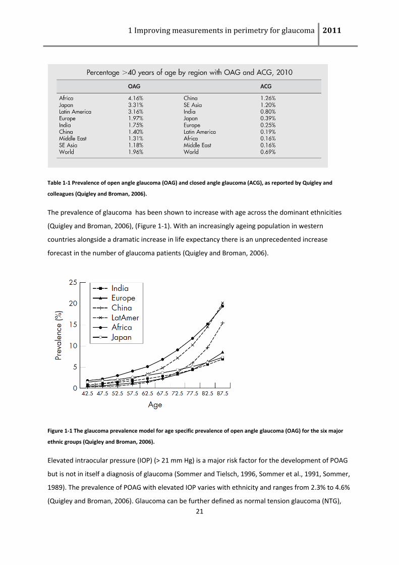
Table 1-1 Prevalence of open angle glaucoma (OAG) and closed angle glaucoma (ACG), as reported by
Quigley and colleagues (Quigley and Broman, 2006). .......................................................................... 21
Figure 1-1 The glaucoma prevalence model for age specific prevalence of open angle glaucoma (OAG)
for the six major ethnic groups (Quigley and Broman, 2006). .............................................................. 21
Figure 1-2 Disparity in measurement scales for an ideal device compared to a typical device. The
orange dashed line represents the normative range. Measures falling to the right of the normative
range make detection possible. The dotted grey lines demonstrate the non-uniformity present in a
typical device. The distance between a and b is less than that between c and d on measurement scale
(x-axis) whereas these are equidistant with the ideal device. .............................................................. 29
Figure 1-3 A schematic showing the line of sight and sensitivity of the hill of vision with respect to
eccentricity, where the brightest white represents the most sensitive area and sensitivity reduces
with eccentricity. ................................................................................................................................... 33
Figure 1-4 Normal hill of vision for contrast sensitivity (white stimulus on a white background) on the
z-axis. Respective luminance values are given for the mean stimulus perceived by the healthy subject
from 0˚-90˚. Beneath there is a diagrammatic example of a patient with pathology (Image courtesy of
M. Monhart). ......................................................................................................................................... 33
Figure 1-5 (A) Goldman type III stimulus (B) the central 24-2 threshold test pattern (right eye) (C)
Suprathreshold testing pattern (right eye). .......................................................................................... 36
Figure 1-6 Short Wave Automated Perimetry stimulus. ....................................................................... 38
Figure 1-7 (A) Frequency Doubling Technology stimulus (B) Frequency Doubling Technology test
pattern location 0-54 indicate left eye test locations, while locations 2-56 indicate right eye test
locations (courtesy of C. Johnson) (C) Suprathreshold screening pattern used in the FDT 1 C-20-5
strategy. ................................................................................................................................................. 39
Figure 1-8 Motion Displacement Test stimulus presentation and test pattern for the right eye......... 40
Figure 1-9 Schematic showing Frequency Defined Form stimuli
http://www.optech.net.au/optech_net_HEP.html. ............................................................................. 41
Figure 2-2 The FOS curve for a subject with reference threshold of 5.5 minutes of arc with the MMDT
stimulus. The green values represent increments of pixels (step size). These steps in intensity values
can be read by tracing down the respective green vertical line. The blue values are the y-value/
proportion seen at the given intensity level (intersection of blue curve and green vertical line to the
left of this value). ................................................................................................................................... 49
1 Improving measurements in perimetry for glaucoma 2011
7
Figure 2-3 The FOS curve for a subject with reference threshold of 5.5 minutes of arc with the MMDT
stimulus. The green values represent increments of pixels (step size). These steps in intensity values
are easily interpreted by tracing down the respective green vertical line. The blue values are the y-
value/ proportion seen at the given intensity level (intersection of blue curve and green vertical line
to the left of this value). ........................................................................................................................ 50
Figure 2-4 Frequency of seeing (FOS) data was collected at the indicated test locations (red markers).
Dummy stimuli were located at blue markers and the fixation target was location at the central point.
Remaining 32 line stimuli were displayed at the indicated locations, but remained stationary for the
duration of the data collection. ............................................................................................................. 52
Figure 2-5 Details of the Psignifit module analysis. Plot A shows the derived lognormal fit to MMDT
data at a single location (+15⁰,+15⁰) for a visually healthy subject. Plot B is the Monte Carlo
generated deviance values of the model; here the fit is indicated with a blue line, and the 95%
Confidence interval (CI) with a red line. Plot C shows the residuals of the fit to the raw data, plot D
gives the Monte Carlo generated deviance values of the residuals of the data (green line) against the
residuals fit is indicated with the green line and the 95% CI with red lines. ........................................ 54
Figure 2-6 An example fit using the Psignifit module on MMDT data (raw data points are represented
with green dots). Data was collected at location (+03⁰, +03⁰) in a healthy observer. The fit returns a
reference threshold of 5.8 minutes of arc (MoA), with a narrow 95% confidence interval of [5.0MoA,
6.9 MoA]. The 95% confidence limits for the 10% and 90% seen points of the curve are also denoted
with boxplots. ........................................................................................................................................ 55
Figure 2-7 Greyscale plots from SAP SITA 24-2 threshold measures taken on 14 glaucomatous
patients, including MD and PSD values (lower right corner). ............................................................... 62
Figure 2-8 Three FOS curves constructed from data collected at a single test location for three
different test subjects (rows) at the location (+03 o,+03 o ) an eccentricity of 4.2 degrees from fixation
target. Row 1 is data collected from a healthy subject, row 2 and 3 contain data collected from mild
and moderate glaucomatous patients respectively. The stimulus intensity (different ranges for each
curve) is given on the x-axis (minutes of arc), the probability of seeing the stimulus is given on the y-
axis (probability). To the right hand side the associated SAP greyscale plot is given with the test
location denoted with a red dot. The red vertical dashed line shows the healthy observers reference
MMDT threshold at this location for comparison with reference threshold of mild and moderate
patient examples. .................................................................................................................................. 63
Figure 2-9 Three FOS curves constructed from data collected at a single test location for three
different test subjects (rows) at the location (-09 o,-09 o) an eccentricity of 12.1 degrees from fixation
target. Row 1 is data collected from a healthy subject, row 2 and 3 contain data collected from mild
and moderate glaucomatous patients respectively. The stimulus intensity (different ranges for each
curve) is given on the x-axis (minutes of arc), the probability of seeing the stimulus is given on the y-
axis (probability). To the right hand side the associated SAP greyscale plot is given with the test
location denoted with a red dot. The red vertical dashed line shows the healthy observers reference
1 Improving measurements in perimetry for glaucoma 2011
8
MMDT threshold at this location for comparison with reference threshold of mild and moderate
patient examples. .................................................................................................................................. 64
Figure 2-10 Three FOS curves constructed from data collected at a single test location for three
different test subjects (rows) at the location (-27o, +03 o) an eccentricity of 27.1 degrees from fixation
target. Row 1 is data collected from a healthy subject, row 2 and 3 contain data collected from mild
and moderate glaucomatous patients respectively. The stimulus intensity (different ranges for each
curve) is given on the x-axis (minutes of arc), the probability of seeing the stimulus is given on the y-
axis (probability). To the right hand side the associated SAP greyscale plot is given with the test
location denoted with a red dot. The red vertical dashed line shows the healthy observers reference
MMDT threshold at this location for comparison with reference threshold of mild and moderate
patient examples. .................................................................................................................................. 65
Table 2-1 A summary of average threshold and slope parameters across glaucoma patient (red) and
visually healthy (green) groups, including standard deviation (STD) of threshold and slope estimates
and the p-value derived using a two sample T-test (threshold) between the groups is also given.
Significant p-values are highlighted in yellow. ...................................................................................... 66
Figure 2-11 Threshold with respect to eccentricity for glaucomatous patients (red circles) and visually
healthy subjects (blue triangles). .......................................................................................................... 67
Figure 2-12 Slope of each FOS collected with respect to eccentricity for glaucomatous patients (red
squares) and visually healthy subjects (blue triangles). ........................................................................ 69
Figure 2-13 The relationship between slope of the sensitivity profile as against reference threshold.
The red (glaucomatous) and blue (visually healthy) solid lines represents a fitted curve to the
respective dataset (of the form 2.69*x^(-0.54)), the dotted lines on either side of the curve represent
the prediction bounds. .......................................................................................................................... 70
Figure 2-14 The relationship between inverse slope of the sensitivity profile as against reference
threshold. The red (glaucomatous) and blue (visually healthy) solid lines represent a fitted line to the
respective dataset, the dotted lines on either side of the line represent the prediction bounds.
Equation of the red fitted line is 0.84x+0.76. For completeness the relationship between interquartile
range and threshold is also given. ......................................................................................................... 71
Figure 2-15 The relationship between interquartile range (width in minutes of arc from the 25% seen
to 75% seen points on the FOS curve) and threshold (minutes of arc) . .............................................. 72
Equation 3-1 Bias at one location .......................................................................................................... 76
Equation 3-2 Precision at one location ................................................................................................. 76
Equation 3-3 Accuracy ........................................................................................................................... 76
Equation 3-4 Test Duration ................................................................................................................... 77
Equation 3-5 Efficiency .......................................................................................................................... 77
1 Improving measurements in perimetry for glaucoma 2011
9
Figure 3-1 Methodology for presentation intensity selection of first presentation of WEBS (red) and
MOBS (green) ........................................................................................................................................ 84
Figure 3-2 A schematic of one possible WEBS tree. Nodes are represented by ovals, recovery points
by diamonds and threshold returned given by the number within the rectangles. Presentation
intensity is given by the number in the centre of each oval. Responses yes (Y) or no (N) from the
previous presentation is given in each oval. All possible search paths are contained within this
diagram. ................................................................................................................................................. 85
Figure 3-3 Summary of the comparative performance of clinical threshold search methods from eyes
of visually healthy subjects. Each blue dot represents the difference between estimated thresholds
using the respective clinical threshold search method against reference thresholds as calculated from
the constructed FOS curves in chapter 2. The black line represents the bias, the dashed black lines
represents the standard deviation, which is inversely proportional to the precision; the red lines
show the trend of estimated threshold with respect to reference threshold. Summary measures are
given in the table (test duration is average seconds per location). ...................................................... 88
Figure 3-4 Summary of the comparative performance of clinical threshold search methods from eyes
of glaucomatous patients. Each blue dot represents the difference between estimated thresholds
using the respective clinical threshold search method against reference thresholds as calculated from
the constructed FOS curves in chapter 2. The black line represents the bias, the dashed black lines
represents the standard deviation, which is inversely proportional to the precision; the red lines
show the trend of estimated threshold with respect to reference threshold. Summary measures are
given in the table (test duration is average seconds per location). ...................................................... 89
Figure 3-5 Number of presentations required to reach termination in visually healthy subjects and
glaucomatous patients. The height of the box represents the inter-quartile range. The median is
shown by the red horizontal line. If the notches (narrower portion) of one box do not overlap with
those of another box this indicates significant difference between the number of presentations
required. ................................................................................................................................................ 90
Figure 3-6 The FOS curve for a subject with threshold of 5.5 minutes of arc with the MMDT stimulus.
The green values represent the number of steps (increments of pixels), required to reach this
stimulus intensity. ................................................................................................................................. 92
Figure 3-7 Schematic showing outcome of 1000 trials with the 1-1 staircase with one reversal
prompting termination and threshold recorded as terminating presentation..................................... 93
Figure 3-8 The outcome of 1000 trials using the 1-1 staircase with two reversals prompting
termination and threshold returned as the last intensity corresponding to the seen response.......... 94
Figure 3-9 A box and whisker plot of 1,000 simulations for each strategy (step size of 1 minute of arc)
for one subject at one location. The red line denotes the mean difference between reference
threshold and estimated threshold (bias), the lower and upper extremes of the box represent the
1 Improving measurements in perimetry for glaucoma 2011
10
25th – 75th centile, and the ends of the whiskers the 5th -95th centiles. The spread of the data
represents the accuracy of the estimated measure. ............................................................................ 96
Figure 3-10 Blue symbols represent outcomes from 1-1 staircase search, green from a 2-1 staircase
search and pink from a WEBS search. Outcomes derived from glaucomatous patients are denoted
with cross and visually healthy subject by a diamond. ......................................................................... 97
Figure 3-11 Mean summary measures from Figure 3-10, for all data denoted ‘all’ on the x-axis, then
for three groupings; 1) where startpoint is within 2.5 minutes of arc of reference threshold, 2)
between 2.5 and 5 minutes of arc, or 3) greater than 5 minutes of arc from reference threshold. Blue
triangles represent outcomes from 1-1 staircases, green triangles outcomes from 2-1 staircases and
pink triangles outcomes from WEBS. .................................................................................................... 98
Figure 3-12 Efficiency calculated for all 5 step sizes and reported mean of all estimated thresholds
and for mean of each group with respect to the distance between startpoint and reference
threshold. 1) where startpoint is within 2.5 minutes of arc of reference threshold, 2) between 2.5 and
5 minutes of arc, or 3) greater than 5 minutes of arc from reference threshold. Blue triangles
represent outcomes from 1-1 staircases, green triangles outcomes from 2-1 staircases and pink
triangles outcomes from WEBS. .......................................................................................................... 100
Figure 4-1 gives a flowchart of the processes which comprise the ESTA method. PTD denotes the
Probability of True damage. ................................................................................................................ 106
Equation 4-1 Functional correlation to structural measures of optic nerve head angle and retinal
distance ............................................................................................................................................... 107
Figure 4-2 Example of initial sweep results, displayed in the grid like format of the 24-2 test pattern.
............................................................................................................................................................. 107
Figure 4-3 Two examples of functional coefficients (upper schematics) are shown. The seed locations
are marked in orange [(-15⁰,15⁰),(+03⁰,-09⁰)], and those correlations greater than 0.65 are marked in
yellow, thus the neighbourhood is highlighted. Below each is the normalized weightings of
neighbours, the seed location is marked in dark green and the neighbours in lighter green. ........... 108
Figure 4-4 Results of the initial sweep (A) are combined with each map of standardised correlations
(single map for location (+03,-09) shown in B) to derive the probability of true damage. ................ 109
Equation 4-2 ........................................................................................................................................ 113
Figure 4-5 Scatter plot of the number of presentations required to reach termination for all 14
visually healthy (green) and 14 glaucoma patients (red), for each suprathreshold strategy (ESTA,
C1/2, MS 1/2 and MS 2/3). Horizontal jitter has been added to help show the distribution of test
duration. A box and whisker plot for each group is superimposed on top of the data points. The
average number of presentations required is stated at the bottom of the graph under the
corresponding group. .......................................................................................................................... 114
1 Improving measurements in perimetry for glaucoma 2011
11
Table 4-1 Summary of agreement in classification between each suprathreshold method (ESTA,
Conventional, Multisampling 1/2 and Multisampling 2/3) and the reference standard of criterion 1.
............................................................................................................................................................. 115
Table 4-2 Summary of agreement in classification between each suprathreshold method (ESTA,
Conventional, Multisampling 1/2 and Multisampling 2/3) and the reference standard of criterion 2.
............................................................................................................................................................. 116
Figure 5-1 Receiver operator characteristic curve for suprathreshold tests on SAP (red line), MDT
(blue line) and FDT (green line). .......................................................................................................... 123
Figure 5-2 The partial receiver operator curve (85%-100% specificity) analysis for each instrument,
highlighting sensitivity at important high levels of specificty. The blue shaded area represents the
95% confidence interval for 95% specificity, while the lighter orange shaded area represents the 95%
confidence interval for 90% specificity. Within both intervals the measures for SAP, MMDT and FDT
overlap to a large extent. .................................................................................................................... 124
Table 5-1 Summary of the sensitivity and specificity values of the three screening perimetric devices.
............................................................................................................................................................. 125
Figure 5-3 Summary of test duration of the three screening perimetric devices. ............................. 126
Figure 5-4 example of clusters of defective locations for cluster size analysis ................................... 129
Table 5-2 Diagnostic characteristics for each instrument. .................................................................. 130
Figure 5-5 ROC curves of HEP, SAP, FDT and MMDT are shown in purple, green, blue and red,
respectively. Numbered points indicate the size of the largest depressed cluster and the
corresponding sensitivity and specificity. ........................................................................................... 130
Figure 5-6 Histogram of the age demographics of subjects attending WGD 2009. ............................ 133
Figure 5-7 Histogram of the distribution of test duration. ................................................................. 135
Figure 5-8 Bar chart of number of test sessions per instrument throughout the day. ....................... 135
Figure 5-9 The distribution of MMDT PTD for attendees of WGD 2009, for Left, Right and max of Right
and Left. ............................................................................................................................................... 136
Figure 5-10 Flow chart of referrals from WGD 2009. .......................................................................... 137
Figure 5-11 Bar chart of the assessment of the performance of the MMDT following phenotyping
with the cut-off criterion PTD of 2.0. .................................................................................................. 138
Table 5-3 Summary of each of positive predictive values and negative predictive values of IOP and
MMDT ESTA. ........................................................................................................................................ 138
1 Improving measurements in perimetry for glaucoma 2011
12
Figure 6-1(A) The measured change in IOS for each subject at baseline (no WOF) and fog filters 1-5.
(B) the age equivalent induced by each WOF across subjects, according to the C- Quant normative
database. This normative database gives the mean and the limits of normality, which have been
translated here into mean predicted age ........................................................................................... 145
Figure 6-2 Shows the Threshold Mean Sensitivity with respect to the (1-4) grade of White Opacity
Filter, where the grey area represents the normative range. It is clear that despite the negative trend
in Frequency Defined Form, Standard Automated Perimetry and Frequency Doubling Technology,
they mainly remain with the normative range of measured values. .................................................. 148
Figure 6-3 (A) Box and whisker plot of the z-scores against the respective increase in stray light, 3
subgroups 0-1.2dB, 1.2dB-1.6dB and 1.6-2.0dB (B) Box and whisker plot of the distribution of TMS
values for each instrument for 3 degress of increases in IOS; 10-50%, 50-100% and 100-200%. The
grey line bisecting each box is representative of the median z-score. The heavy black lines across the
graph show the confidence limits for the normative range corresponding to the 75% cut-off and 95%
cut-off. (* denotes a significant difference p<0.01, ** p<0.0001, ANOVA two way test) .................. 150
Figure 6-4 Scatterplot of standardised z-scores with respect to the change in stray light. Each symbol
represents a different instrument. Each marker shows a mean standardised z-score for one subject,
with one instrument and one filter. .................................................................................................... 151
Figure A-1 Example of ESTA MMDT graphical output showing an upper hemifield defect (right eye).
............................................................................................................................................................. 163
Figure. A- 2 The Optic nerve head location, in degrees, for each visual field point of the Standard
Automated Perimetry 24-2 program ................................................................................................... 164
Figure A-5 Detailed flow chart of ESTA, PTD denotes the probability of true damage, RA the results
array, WA the weighting array, the presentation intensity level on that sweep and
the upper and lower limits for retesting at the j the location. ..................................................... 169

1 Improving measurements in perimetry for glaucoma 2011
13
Acknowledgements
I would like to acknowledge the help and guidance of my supervisors in particular Professor David
Crabb, for his patience and help. I would also like to thank Dr J Oleszczuk for her careful proof
reading of this thesis in preparation for submission.
This work was chiefly supported by the Special Trustees of Moorfields Eye Hospital and an
unrestricted research award from Heidelberg Engineering.
Declaration
This thesis has been completed solely by the candidate, Ciara Bergin.
It has not been submitted for any other degrees, either now or in the past, where work contained
within it has been previously published this has been stated in the text.
All sources of information have been acknowledged and references given.
I hereby consent to allow the librarian of City University London to copy in whole or in part the thesis
for study purposes.
1 Improving measurements in perimetry for glaucoma 2011
14
Abstract
Improving measurement in perimetry for glaucoma
Ciara Bergin (City University London)
Glaucoma is a leading cause of visual impairment and, if untreated, irreversible blindness. Perimetry is the clinical tool for assessing the functional ‘seeing’ part of the field of view (visual field) and is widely used in the detection and clinical monitoring of glaucoma. These measurements rely on a psychophysical response making them inherently variable. This measurement noise can disguise both disease pathology and progression.
The work described in this thesis aims to improve the quality of perimetric measurements. The platform for this is the Moorfields Motion Displacement Test (MMDT), a perimetric test that uses unconventional test stimuli and can be delivered on an ordinary computer monitor. Specifically, this thesis describes efforts to develop novel, mathematically derived, test algorithms, designed to be used with the MMDT. The performance of these new testing methods is assessed using pilot studies involving patients and visually healthy people, computer simulation and interim results from a large prospective clinical study. One of these test algorithms, the Enhanced Suprathreshold Testing Algorithm [ESTA] provides shorter test duration, making it attractive for case-finding and screening for glaucoma, without seemingly negatively affecting diagnostic precision, and has become patented technology. Another bespoke test algorithm (Weighted Binary Search; WEBS) provides a threshold test for the MMDT.
The thesis also describes a study examining the resistance of several newer clinical perimetric instruments to the optical artefact of stray light that might be caused by media opacity. This is clinically important because cataract and degraded optical media is a leading cause of false-referral for glaucoma. This work, being the first of its kind, indicates that the MMDT has greater resilience to simulated effects of media opacity compared with other clinically used devices.

1 Improving measurements in perimetry for glaucoma 2011
15
Acronyms
APE Adaptive Probit Estimation
ASTA-Std Standard Adaptive Staircase Thresholding Algorithm
BP Blood Pressure
C 1/2 Conventional Suprathreshold
CC Correlation Coefficients
CCT Central Corneal Thickness
CI Confidence Interval
DLS Differential Light Sensitivity
EGS European Glaucoma Society
ESTA Enhanced Suprathreshold Testing Algorithm
FDT Frequency Doubling Technology
FDF Frequency Defined Form
FFS Full Field Simulator
FN False Negative
FoS Frequency of Seeing
FP False Positive
FT Full Threshold
GAT Goldmann Applanation Tonometry
GHT Glaucoma Hemifield Test
GON Glaucomatous Optic Neuropathy

1 Improving measurements in perimetry for glaucoma 2011
16
GRP Grating Resolution Perimetry
HEP Heidelberg Edge Perimeter
HFA Humphrey Field Analyzer
HoV Hill of Vision
HRT Heidelberg Retinal Tomograph
IOP Intraocular pressure
IOS Intraocular Straylight
MD Mean Defect
MMDT Moorfields Motion Displacement Test
MS 2/2 Multisampling Suprathreshold two out of two criterion
MS 2/3 Multisampling Suprathreshold two out of three criterion
MOBS Modified Binary Search
MOCS Method of Constant Stimuli
NTG Normal Tension Glaucoma
ONH Optic Nerve Head
ORS Observer Response Simulator
PACG Primary Angle Closure Glaucoma
PD Pattern Deviation
PDF Probability Density Function
PICS Perimetry Instrument Comparison Study
POAG Primary Open Angle Glaucoma
PP Pulsar Perimetry
1 Improving measurements in perimetry for glaucoma 2011
17
PSD Pattern Standard Deviation
ROC Receiver Operator Characteristic
RNFL Retinal Nerve Fibre Layer
SAP Standard Automated Perimetry
SITA Swedish Interactive Threshold Algortihm
SLv Standard Local Variance
ST Suprathreshold
SWAP Shortwave Automated Perimetry
TD Total Deviation
TOP Tendency Oriented Perimetry
VF Visual Field
WEBS Weighted Binary Search
WOF White Opacity Filter
YAAP Yet Another Adaptive Procedure
ZEST Zippy Estimation of Sequential Testing
1 Improving measurements in perimetry for glaucoma 2011
18
1 Introduction
1.1 Overview of thesis
In short, this thesis describes the development of two novel test strategies to improve visual field
assessment in glaucoma and a novel experiment examining the resistance of four clinical perimetric
instruments to the simulated effects of cataract. The test strategies developed within this thesis are
designed to be applicable to any perimetric instrument but were initially motivated by the practical
requirements of the Moorfields Motion Displacement Test (MMDT).
The MMDT is a software program which provides a test of the field of vision. It was developed from
the principles of a single-location MMDT (Fitzke et al., 1987). The test was refined and expanded to a
multi-location format prior to the start of this thesis (Verdon-Roe, 2006, Moosavi, In submission; MD
Thesis) (www.moorfieldsmdt.co.uk).
Chapter one provides an introduction to glaucoma diagnosis and management. A brief overview of
the risk factors and epidemiology of the disease is given, followed by an outline of the instruments
used for detection and monitoring of the disease. This leads to a discussion on the role of
measurement error, which causes misclassification errors, increases test variability and lowers
repeatability. This in turn leads to a discussion of the importance of reducing noise in perimetry
measures for glaucoma management. The chapter is concluded with an overview of newer
perimetric instruments.
Chapter two describes the development of a computer based ‘patient simulator’ via the collection of
so called Frequency of Seeing data on the MMDT, for perimetric testing which is used in chapters
three and four. Chapter three of the thesis outlines threshold testing algorithms used in perimetry
and discusses which of these provides a suitable method for the MMDT. Several clinical search
methods have been previously depicted in the literature; primarily these have the disadvantage of
being significantly slower, in terms of test time, for glaucoma patients than for subjects with healthy
vision. This chapter reports on the development of an alternative search method (threshold
algorithm), adapting a previously reported algorithm.
1 Improving measurements in perimetry for glaucoma 2011
19
Chapter four describes the development of a completely novel fast suprathreshold strategy which
implements spatial information contained within the visual field. The aim of this testing method is to
provide a quick test of the visual field making it potentially suitable in screening and case finding.
Chapter 5 illustrates how the two test strategies, as implemented on the Moorfields MMDT, were
used in a prospective study comparing different perimetric instruments. Also the outcome of a
screening type study implementing the MMDT suprathreshold test is reported.
The presence of cataract is an additional difficulty in glaucoma management for detection and
follow-up. In the screening or case-finding scenario, false referrals contribute a large proportion of
the referred cases (Bowling et al., 2005). When truly trying to identify glaucoma, especially in an
elderly population, the effect of cataract is a serious confounder to glaucoma patient care, which
underlines the importance of the estimation of effect of cataract on newer types of perimetric
stimuli. Chapter 6 of this thesis consists of a novel investigative study which was undertaken to
examine the resistance of several newer clinical perimetric instruments to the effects of induced
increases in stray light by comparison with standard automated perimetry (SAP), which is a measure
of differential light sensitivity. From a clinical perspective, this may be regarded as a simulation of the
effects of cataract on clinical perimetric measures. Chapter 7 concludes with a brief summary of the
prospective projects arising from discoveries made within this PhD.
1.2 Classification of Glaucoma
Glaucoma is a collective term for a complex group of conditions that have a common end point of
progressive optic neuropathy. Glaucomatous optic neuropathy (GON) is characterized by distinctive
patterns of structural changes at the optic nerve head (ONH) and of the retinal nerve fibre layer
(RNFL) with associated loss of visual function.
The conventional classification of primary glaucoma is by the anatomical configuration of the
drainage system of the eye: primary open angle glaucoma (POAG), where the drainage angle is non-
occludable, and primary angle closure (PACG), where the drainage angle is occluded. Secondary
glaucoma may be due to a variety of processes, which include, for example, steroid induction,
pseudoexfoliation, pigment dispersion, uveitis, diabetes (neovascular), central retinal vein occlusion
(neovascular), significant hyphema or trauma.
1 Improving measurements in perimetry for glaucoma 2011
20
The modern concept of glaucoma is that it is a primary neurodegenerative disease of the optic nerve,
with complex ocular and systemic contributions, which may be influenced by genetic and
environmental factors.
1.2.1 Presentation of Glaucoma
Within the UK there is no systematic screening program for glaucoma. Case finding usually occurs
during routine eye care examination. Therefore, optometrists initiate more than 96% of glaucoma
case referrals (Sheldrick et al., 1994, Bell and O'Brien, 1997). However, it has been estimated that up
to 63% of referrals are false positive (Lockwood et al., Sheldrick et al., 1994, Bowling et al., 2005),
which results in wastage of resources and unnecessary anxiety and inconvenience to the patient.
Training can reduce the false positive rate (Henson et al., 2003, Patel et al., 2005), but this has not
been implemented on a large scale. A recent Health Technology Assessment report by Burr and
colleagues (Burr et al., 2007) states that up to 67% of glaucoma in the UK is undiagnosed, the
insidious nature of the disease being a major confounder to its detection.
POAG has a gradual and painless progression. Due to the sensory adaptation to the gradual loss of
visual field the patient is often unaware of disease presence until an advanced stage has been
reached (Bunce and Wormald, 2006, Fraser et al., 1999). If glaucoma is detected early the prognosis
is good and the probability of bilateral blindness is low (Quigley and Broman, 2006, Chen, 2003,
Munoz et al., 2000, Quigley, 1999, Blomdahl et al., 1997).
1.2.2 Epidemiology and risk factors
Approximately 2.7% of the global population is affected by glaucoma (Table 1-1); there are large
differences in reported rates of prevalence with respect to sex, ethnicity and age (Figure 1-1). Two
per cent of the population is affected by PAOG and 0.7% by PACG. Those of African racial origin are
more than twice as likely to develop PAOG as Europeans. Chinese and South East Asians are 5 times
as likely to develop PACG as Europeans.
1 Improving measurements in perimetry for glaucoma 2011
21
Table 1-1 Prevalence of open angle glaucoma (OAG) and closed angle glaucoma (ACG), as reported by Quigley and
colleagues (Quigley and Broman, 2006).
The prevalence of glaucoma has been shown to increase with age across the dominant ethnicities
(Quigley and Broman, 2006), (Figure 1-1). With an increasingly ageing population in western
countries alongside a dramatic increase in life expectancy there is an unprecedented increase
forecast in the number of glaucoma patients (Quigley and Broman, 2006).
Figure 1-1 The glaucoma prevalence model for age specific prevalence of open angle glaucoma (OAG) for the six major
ethnic groups (Quigley and Broman, 2006).
Elevated intraocular pressure (IOP) (> 21 mm Hg) is a major risk factor for the development of POAG
but is not in itself a diagnosis of glaucoma (Sommer and Tielsch, 1996, Sommer et al., 1991, Sommer,
1989). The prevalence of POAG with elevated IOP varies with ethnicity and ranges from 2.3% to 4.6%
(Quigley and Broman, 2006). Glaucoma can be further defined as normal tension glaucoma (NTG),
1 Improving measurements in perimetry for glaucoma 2011
22
where IOP is < 21 mm Hg. From the Rotterdam 10 year follow-up study it is estimated that with every
1mmHg increase in IOP there is an 11% increase in risk of developing glaucomatous vision loss
(Czudowska et al., 2010).
Family history of glaucoma is a recognised risk factor for glaucoma. However, the assessment of
family history is subject to error where it is reliant on patient self-reporting (Craig et al., 2001, Tielsch
et al., 1994, Mitchell et al., 2002). Since the prevalence of POAG in first-degree relatives is low, this
suggests that not a single-gene but rather a multi-gene combination is responsible for the disease
(Garway-Heath, 2000). Several large family gene studies are currently being conducted to explore
this further, the results of which may have large ramifications for the screening and treatment of
glaucoma. Systemic factors such as hypertension (Sommer and Tielsch, 2008, Langman et al., 2005)
and diabetes (Frank and Dieckert, 1996, Tan et al., 2009) have also been shown to be associated with
glaucoma and more recently ocular biometry (Bourne et al., 2008, Kuzin et al., 2010, Perera et al.,
2010).
1.3 Detection and monitoring of Glaucoma
Different measurements are acquired during clinical examination for the detection and monitoring of
glaucoma, namely IOP measurement and gonioscopy for the assessment of the related structures
with respect to drainage or blockage, the health of the optic nerve head (referred to as structural
measures) and assessment of the visual field (functional measures). No single measure provides
conclusive evidence of presence or absence of glaucoma, nor is one measure sufficient for the
monitoring of the disease. Instead, the combination of evidence from all three groups of measures is
used to determine the presence and to monitor the progression of the glaucomatous damage.
Conventional IOP measures are taken with the current reference standard test, Goldmann
applanation tonometry (GAT) (Kotecha et al., 2010). The measure is then assessed as to whether it is
within or outside normal limits. 95% of the healthy European population has IOP≤21mmHg (95.4% of
the population had pressure below 22mmHg). Evidence of iridocorneal angle narrowing (including
evidence of previous apposition (peripheral anterior synechiae)), closure or blockage to the
trabecular mesh work (e.g. pigment dispersion) should also be investigated during routine
examination using the current gold standard of gonioscopic inspection in dark adaptation.
1 Improving measurements in perimetry for glaucoma 2011
23
A high IOP reading (>21mmHg; ocular hypertension) can be an indicator of glaucoma. The higher the
IOP reading the greater the probability of the disease (Davanger et al., 1991, Klein et al.,
1992).Tracking the level of IOP when following a patient provides important clinical information. An
increase in the IOP reading can indicate that medication is no longer yielding the desired efficacy.
However, all IOP measures are subject to inter/intra observer variability and diurnal changes or
associated measurement error (Kotecha et al., 2005, Sudesh et al., 1993, Kotecha et al., 2010).
The ONH (or optic disc) contains the neuro-retinal rim and the optic cup. The neuro-retinal rim is the
gathered retinal nerve bundles leaving the eye and is delimited peripherally by the edge of the RPE
and internally by the cup. The cup is the depression at the centre of the disc. As nerve fibres are lost
the amount of space taken up by the neuro-retinal rim reduces. The health of the ONH is assessed
clinically under slit lamp examination within routine glaucoma care. This is often summarised with
the parameter of cup to disc ratio, where a high ratio would represent an unhealthy disc (Armaly,
1969). Since this is a subjective measure there are associated variability issues. When monitoring for
glaucomatous change, a subjective measure such as cup to disc ratio is not sensitive to subtle
changes, instead large changes to the shape of the ONH, such as significant cupping, notching or
other changes such as haemorrhage must be noted. Most likely lesser but significant changes/losses
e.g. the cup to disc ratio changes from 0.70 to 0.80 will be disregarded as inter/intra-observer
differences.
Imaging devices using different optical techniques can also be used to assess the ONH and RNFL
thickness such as scanning laser ophthalmoscope (SLO) as in the commercially available Heidelberg
Retinal Tomograph (HRT)(Heidelberg engineering, Heidelberg Germany), scanning laser polarimetry
(SLP) as is implemented in the GDx (Carl Zeiss Meditec, Dublin, CA, USA), and ocular coherence
tomography (OCT) as with the Cirrus (Carl Zeiss Meditec, Dublin, CA, USA) or the RT-VUE (Optovue,
Fremont, CA, USA)(Greenfield and Weinreb, 2008, Townsend et al., 2009).
The HRT is an example of SLO technology and is used in the assessment and management of
glaucoma (Chauhan, 1996, Mikelberg et al., 1995, Zangwill et al., 2004, Zinser et al., 1989). In the
case of the HRT the neuroretinal rim area of the ONH can be assessed (statistically) to be within or
outside normal limits; this can be done within the software of the instrument, using the Moorfields
multivariate regression analysis (MRA)(Wollstein et al., 1998). The HRT is also useful for monitoring
for progression (Chauhan et al., 2000, Patterson et al., 2005). Another advantage that imaging
1 Improving measurements in perimetry for glaucoma 2011
24
methods such as these have is that little patient co-operation is required. This is a less subjective
measure.
Functional measures are unappealing clinically as they are time consuming and sometimes difficult
for patients (Gardiner et al., 2008). Despite these disadvantages, in terms of glaucoma management
visual field assessment is very important. This is because the classification of the ONH or the level at
which the IOP stands cannot provide any functional information and maintaining functional health is
the primary aim of glaucoma treatment (European glaucoma society guidelines, 2009).
Visual function loss is the lessening of ability to perceive/process visual information from the full
healthy visual function profile. The healthy visual function profile can be established from the normal
population. Comparison between the measured profile and the healthy profile is performed to
detect loss, this may be diffuse or local or a combination of both. ‘Progression’ or further visual
function loss is deterministic in treatment changes.
Treatment of glaucoma currently involves controlling IOP levels. This is achieved medically or
surgically or using a combination of both. The method is determined based on patient dependent
factors such as compliancy (Robin et al., 2007), IOP control needed, and/or whether maximal
tolerated treatment is reached. A moderate drop in IOP has been shown to change the course of
progression of visual field loss (Chauhan et al., 2010).
1.4 Measurement error in glaucoma assessment
All the clinical measures in glaucoma are subject to inter and intra test measurement noise. The
following provides a short overview.
1.4.1 IOP measurements
Apart from the large inter-observer and inter-visit variability inherent to this method of assessment
there are some less obvious sources of measurement error, where careful consideration has yielded
positive results with respect to reducing measurement noise.
1 Improving measurements in perimetry for glaucoma 2011
25
The normative cut off changes with age and with race are as previously described in Figure 1-1.
However less obvious was the different increment of IOP with age with respect to race (Klein et al.,
1992). Generally this was understood to be approximately 0.03mmHg per year as these limits were
originally established for a mixed population (Qureshi, 1995). With the introduction of race specific
normative cut offs and functions of change with respect to age, classification was significantly
improved. In Japanese populations for example, on switching to race specific database, significant
differences in the classification were made. In this population there is a much lower average IOP
(11.5mmHg) and a lower increase with age of 0.02mmHg per year (Nuramuro et al, 1999).
The GAT method of measuring IOP assumes a constant central corneal thickness (CCT) of
approximately 520 microns. The recent introduction of calibrating IOP according to CCT provides a
means of adjustment for the related measurement error. Previously, no allowance was made for
CCT, resulting in subjects with thicker CCT (> 600 microns) being more likely to be classified as having
raised IOP. Conversely, subjects with thin CCT were more likely to be wrongly classified as NTG
(Brusini et al., 2000, Brandt et al., 2001, Copt et al., 1999, Shah et al., 1999). The newly introduced
DCT (Pascal dynamic contour tonometer DCT; Swiss Microtechnology AG, Port, Switzerland) employs
a correction for CCT. On examination it shows similar reproducibility to GAT, however the inter
observer noise is significantly reduced (Kotecha et al., 2010).
In terms of assessing the structure of health/effectiveness of aqueous drainage pathways the large
inter-observer variability in the standard clinical setting associated with the current gold standard
method of clinical assessment (gonioscopy) is clear as it currently remains a purely subjective
measure (e.g. estimate of iridiocorneal angle in degrees (0⁰-40⁰). New measurement techniques such
as that provided by the anterior segment optical coherence tomography (Visante; Carl Zeiss
Meditec, Dublin, CA, USA) may offer automation of this assessment, providing objective
measurements in years to come (Kim et al., 2009).
1.4.2 Structural measurements
The ability of clinicians to detect glaucomatous eyes using subjective evaluation of ONH appearance
is limited with the direct ophthalmoscope, fundus photography and other similar tools. The use of
imaging systems to aid diagnosis and follow-up of POAG is becoming more widespread. Examples of
1 Improving measurements in perimetry for glaucoma 2011
26
these are the HRT (Heidelberg engineering, Heidelberg Germany), GDx (Carl Zeiss Meditec, Dublin
CA, USA) and RT-VUE (Optovue, Fremont, CA, USA). Studies have shown that whilst none of these
systems are likely to perform better than a glaucoma specialist clinician viewing stereo-photographs,
they can all perform at a similar level and have the potential to aid detection and monitoring of
POAG (e.g. Reus et al., 2007).
Measurement error plays a significant role in the ability to detect change using an optical imaging
device. Much of the responsible noise stems from image acquisition, which takes two forms: inter-
image misalignment due to pulse, head movements, cataract/media opacity etc. (Orgul et al., 1996,
Chauhan and McCormick, 1995, Kremmer et al., 2003) and poor instrument to eye alignment which
results in poorly illuminated images or magnification errors (Garway-Heath et al., 1998).
Imaging techniques have quickly gained high resolution and continue to reduce noise; the large
strides undertaken have resulted in a common misconception that they will lead to next to perfect
images and measures of the optic nerve head and thus a gold standard classification. However, the
images obtained will always be far less than perfect, since some measurement noise will likely
remain. Auto calibration and alignment algorithms have succeeded in significantly reducing image
acquisition noise but it remains difficult to remove this noise completely (for example see section
1.5). Detecting change between images will also remain difficult as any change or loss will have to be
greater than expected measurement noise and aging effects (Chang and Budenz, 2008a, Chang and
Budenz, 2008b).
Structural measures are heavily reliant on normative databases for classification, which is a
disadvantage in the detection of early damage. Early damage is likely to be on the less depressed end
of the measurement scale where the normal population will share the same measures. Therefore
with the current statistical cut-off values of 95%, 98%, 99% and 99.5% employed within most clinical
instruments this “loss” is easily overlooked. Until classification no longer relies on normative
populations, there will likely be considerable misclassification error.
1.4.3 Function
A single visual function assessment can produce an unreliable measure, because of its dependency
on the patient responses. In a visually healthy patient, responses will fluctuate according to fatigue,
1 Improving measurements in perimetry for glaucoma 2011
27
attention and understanding of the test as well as true retinal sensitivity (Henson and Emuh, 2009,
Anderson and McKendrick, 2007, Marra and Flammer, 1991, Johnson et al., 1988). In a glaucomatous
patient these fluctuations are likely to be much greater, and will increase with depth and/or extent of
loss (Artes et al., 2005, Spry et al., 2001), with additional variability along the edges of deficits (Wyatt
et al., 2007).
The presence of ocular media opacity (e.g. cataract) can mimic visual function loss (Superstein et al.,
1999, Moss et al., 1995, Siddiqui et al., 2007, Carrillo et al., 2005, Siddiqui et al., 2005, Matsumoto et
al., 1997). Depending on the type of ocular media opacity present e.g. different types of cataract
(Chylack Jr et al., 1993) focal or diffuse loss can be observed in visual functional assessments. Unlike
glaucoma, the visual functional loss associated with cataract is reversible with phacoemulsification;
therefore it is important to be able to differentiate between them. Efforts have been made to
achieve this (Åsman and Heijl, 1994).
Since both glaucoma and cataract are age related, it is not uncommon for them to occur in tandem.
The advance of cataract development in a glaucomatous patient can mask glaucomatous visual loss
progression, which confounds glaucoma monitoring (Siddiqui et al., 2007, Carrillo et al., 2005,
Siddiqui et al., 2005, Matsumoto et al., 1997). For example, in advanced glaucoma where surgical
interventions are more common, secondary cataract is an associated risk (Hylton et al., 2003, Gedde
et al., 2007b, Gedde et al., 2007a, Borisuth et al., 1999) and can confound the assessment of the
efficacy of the intervention in these high risk patients.
Clinical threshold search methods in functional testing are designed to find the point of subjective
equivalence, at which the subject is equally likely to provide a seen or unseen response, otherwise
known as threshold. The method used to search for threshold introduces bias and variability in
measures of both visually healthy subjects and glaucomatous patients (Turpin et al., 2003, Turpin et
al., 2002b, Bengtsson and Heijl, 2003, Bengtsson and Heijl, 1999b, Bengtsson and Heijl, 1999a).
The depth of the deficit is strongly associated with the amount of variability in a given measure of
retinal sensitivity (Henson et al., 2000, Chauhan et al., 1993, Spenceley and Henson, 1996). Therefore
given a threshold estimated by a clinical search method there is a distribution of thresholds which we
could reasonably expect this threshold estimate to originate from (interpretation error)(King-Smith
et al., 1994, Treutwein, 1995, Wichmann and Hill, 2001a). For change in a threshold measure to be
significant the underlying distributions associated with interpretation error should not overlap,
1 Improving measurements in perimetry for glaucoma 2011
28
however in clinical perimetry these distributions are so wide, that this is unlikely to occur until a large
degree of damage has occurred.
According to Swanson and colleagues, a true reduction in sensitivity from 33dB to 31dB, which is a
loss of 2dB, would equate to the loss of over 50% of ganglion cells (Swanson et al., 2004). However
this measure of 31dB would remain well inside the normative range of a young visually healthy eye at
a central location and thus with the current methodologies would not be isolated as a damaged
location. Considering the test retest variability at this end of the range (SD~±2dB, (Artes et al.,
2002b)), it is clear that a true reduction of 2dB would be indistinguishable from measurement noise.
The difference between two assessments of a given visual field must be greater than sources of
measurement noise, in addition to the possible depression in retinal sensitivity associated with aging
over follow-up, before any further depression in sensitivity is detectable. Depending on the innate
measure of function or structure in any given patient (thick RNFL versus thin RNFL, high sensitivity
versus low sensitivity), functional assessment or structural assessment likely will detect loss in
different orders to one another. This is a major confounder when dealing with individual patients as
the category to which they belong is unknown. One category of patients encompasses those with
innate lower sensitivities and thinner RNFL, when disease presence/progression is detected it is likely
to detected on both functional and structural measures. Conversely, loss in those subjects with
glaucoma but with innate high retinal sensitivity and thick RNFL are unlikely to be detected as
glaucoma sufferers until significant reductions have occurred. This idea could also explain the lack of
agreement between functional and structural measures; those with innate lower sensitivity and
thick RNFL are likely to be detected on functional loss, while those with innate higher sensitivity and
thinner RNFL are likely to be detected with structural loss first.
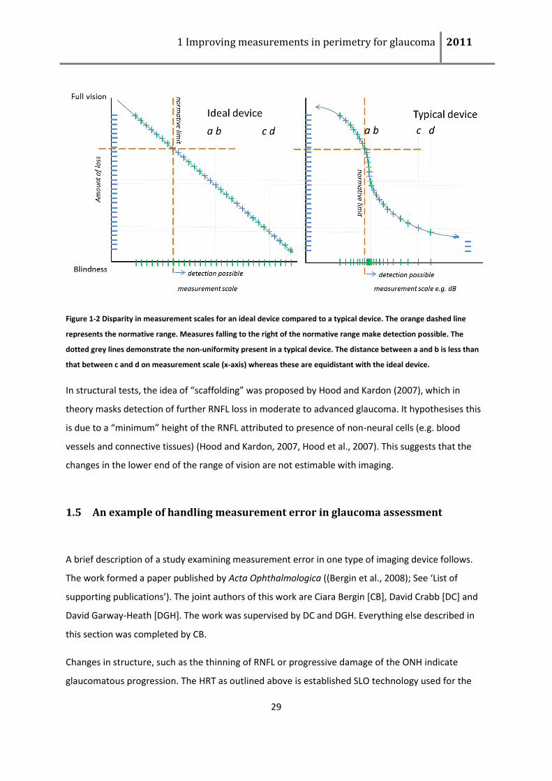
The lack of uniformity in the measurement scales is another large contributor to measurement noise.
With an ideal device the complete scale of vision, from full vision to blindness should be covered,
with uniformity. In typical structural and functional tests there has been no calibrating of
measurement scales, so there is no reason to expect uniformity or high correlations between
measures. Most likely adjacent increments of visual loss will sometimes fall far apart (c and d), while
others far within a small range (a and b) on the measurement scale (see Figure 1-2). This would in
part explain the large variability at the lower end of SAP estimates (<15dB)(Henson et al., 2000).
1 Improving measurements in perimetry for glaucoma 2011
29
Figure 1-2 Disparity in measurement scales for an ideal device compared to a typical device. The orange dashed line
represents the normative range. Measures falling to the right of the normative range make detection possible. The
dotted grey lines demonstrate the non-uniformity present in a typical device. The distance between a and b is less than
that between c and d on measurement scale (x-axis) whereas these are equidistant with the ideal device.
In structural tests, the idea of “scaffolding” was proposed by Hood and Kardon (2007), which in
theory masks detection of further RNFL loss in moderate to advanced glaucoma. It hypothesises this
is due to a “minimum” height of the RNFL attributed to presence of non-neural cells (e.g. blood
vessels and connective tissues) (Hood and Kardon, 2007, Hood et al., 2007). This suggests that the
changes in the lower end of the range of vision are not estimable with imaging.
1.5 An example of handling measurement error in glaucoma assessment
A brief description of a study examining measurement error in one type of imaging device follows.
The work formed a paper published by Acta Ophthalmologica ((Bergin et al., 2008); See ‘List of
supporting publications’). The joint authors of this work are Ciara Bergin [CB], David Crabb [DC] and
David Garway-Heath [DGH]. The work was supervised by DC and DGH. Everything else described in
this section was completed by CB.
Changes in structure, such as the thinning of RNFL or progressive damage of the ONH indicate
glaucomatous progression. The HRT as outlined above is established SLO technology used for the
1 Improving measurements in perimetry for glaucoma 2011
30
examination of the ONH and surrounding RNFL (Chauhan, 1996, Mikelberg et al., 1995, Zangwill et
al., 2004, Zinser et al., 1989); HRT is a useful tool for diagnosis and valuable in patient follow up by
assessing structural change of the ONH by using series of images acquired over time. Analysis of a
series of HRT images is done clinically to help distinguish between progressing glaucomatous patients
and non-progressing patients. However, these images are not identically scaled versions of the true
ONH and are affected by measurement variability during image acquisition (intra-scan noise) and
between the visits in follow-up (inter-scan noise). For example, scan-resolution is limited by the
optics of the human eye; the scanning laser must past through the tear film, cornea, lens and
vitreous humour to reach the ONH; these media produce wave aberrations that degrade the
resulting image (Artal et al., 2001) and add measurement noise. A number of other factors also
contribute to the measurement noise including eye movements, pupil size (Artal et al., 2001, Zangwill
et al., 1997), optic disc size (Iester et al., 1997), changes in intra-ocular pressure, placement of the
contour line (Orgül S et al., 1995) and the use of a reference plane in generating stereometric
parameters (Strouthidis et al., 2005a, Burk et al., 2000) and even the cardiac cycle (Chauhan and
McCormick, 1995).
The new image alignment algorithm was introduced as part of the HRT3 software (version 3.0.2.0)
and the exact detail is proprietary. The aim of this study was to examine the impact of this new
alignment algorithm on the inter-scan variability in series of HRT images, focusing on the
improvements in repeatability of global stereometric parameters (such as neuroretinal rim area
measurements) and also on the variability in the estimated height measurements at each pixel in a
series of images.
HRT image series from 124 patients with glaucoma or ocular hypertension were made available
from previously reported studies (Strouthidis et al., 2003, Strouthidis et al., 2005b, Strouthidis et al.,
2006a) and were re-processed with the old and new image alignment algorithms. Improvements
afforded by the new alignment algorithm were examined by considering statistically significant
improvement in repeatability of specific stereometric parameters (SP), namely Rim Area (RA), Rim
Volume (RV), Cup Volume (CV) and Cup Shape Measure (CSM). A further comparison was made by
examining reduction in the variability of pixel-by-pixel height measures within image series.
In some HRT image series the new algorithm automatically corrected obvious misalignment events
that occurred with the previous algorithm. However, average improvement in repeatability of the
SPs in HRTI image series was not statistically significant (p=0.13) and there was no statistically
1 Improving measurements in perimetry for glaucoma 2011
31
significant reduction in pixel-by-pixel height measurement variability (p=0.73). In HRTII image series,
there was evidence of improvement, on average, in the repeatability of some parameters (RA;
p=0.01, RV; p=0.02, CSM; p=0.05), but not in CV (p=0.22). There was, however, a large reduction in
pixel-by-pixel variability in HRT II image series (p<0.001). Therefore this study, only briefly described
here, revealed some evidence to show that the new algorithm improved repeatability.
1.6 Impact of glaucoma
The loss of nerve fibre layer caused by glaucoma, manifests in structural damage at the optic nerve
head. Considerable RNFL loss results in repeatable measurable visual function loss, manifesting as
depression of sensitivity locally and/or globally. In a glaucomatous eye this loss can progress to
severe visual impairment over time, including the possibility of blindness. As visual function is lost,
the quality of life is negatively affected.
Glaucoma has a major impact on quality of life. According to the European Glaucoma Society, the
goal of glaucoma treatment is to “maintain the patient’s visual function and related quality of life at a
sustainable cost”… “Quality of life is closely linked with visual function and overall patients with early
to moderate glaucomatous damage have good visual function and modest reduction in quality of
life”. To ensure that the functional loss remains early to moderate for the duration of life expectancy,
it is important to detect glaucoma as early as possible. With expected increase in prevalence the
balance between cost effectiveness and early detection and treatment is under review (Burr et al.,
2007).
A reference standard for automated glaucoma detection has not yet been established, but will be
required to facilitate the possibility of glaucoma screening (Hernandez et al., 2008). Currently,
significant damage of structure or function must be present, with the additional requirement of
disease progression detection before diagnosis confirmation (in early glaucomatous cases)
(Guidelines of European Glaucoma Society (EGS) 3rd edition). Due to the innate structures of the
population, as outlined above, it is unlikely that structural measures alone will achieve the
appropriate levels of sensitivity or specificity required for automated case detection. Ideally
detection of damage to both structure and function should determine disease presence; however the
weak relationship between structural measures and functional measures in early glaucomatous cases
1 Improving measurements in perimetry for glaucoma 2011
32
continues to impede a combined approach (Hood and Kardon, 2007, Gardiner et al., 2005, Bowd et
al., 2006). Significant reductions to error in both measures would be required to allow this.
Since a reduction in visual function is deterministic in treatment changes it will continue to serve as
an endpoint for clinical trials. The guidelines for treatment of glaucoma aim at preserving visual
function and avoiding visual impairment – it is reasonable that visual function assessment will remain
paramount in glaucoma care. Furthermore, if glaucoma screening is to be viable, more efficient and
reliable visual functional assessment will be required. Therefore, it is clear that all possible
reductions in measurement noise of functional measures should be pursued as vigorously as those in
structural measures.
1.7 Perimetry
The visual field (VF) was defined by Tate and Lynn (Tate and Lynn, 1977) ‘as all the space that one eye
can see in an instant’. Perimetry is defined as the study of the visual field (VF). Vision is most
sensitive in the line of sight (Henson, 1993). As field of view extends to the periphery, the sensitivity
reduces. From the line of sight the field of view extends 60˚ upwards, 75˚ downwards, 100˚
temporally and 60˚ nasally. The shape and sensitivity of the visual field can be described
geometrically by what is known as the hill of vision. In Figure 1-3 the height of the hill is
demonstrated by the luminance level, with the dark sections representing areas of no vision and the
brightest areas corresponding to the areas of best vision. In healthy eyes there are additional
components affecting the assessment of the hill of vision, the position of the blind spot and the
horizontal streak. This is due to the changes in the underlying ganglion cell mosaic (Dacey, 1993,
Curcio et al., 1991, Thibos, 1998). Furthermore, in eyes with pathology, any number of changes can
be made to the shape of the hill of vision (Weber and Rau, 1992, Chauhan et al., 1993)(Figure 1-4).
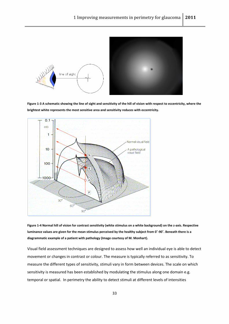
1 Improving measurements in perimetry for glaucoma 2011
33
Figure 1-3 A schematic showing the line of sight and sensitivity of the hill of vision with respect to eccentricity, where the
brightest white represents the most sensitive area and sensitivity reduces with eccentricity.
Figure 1-4 Normal hill of vision for contrast sensitivity (white stimulus on a white background) on the z-axis. Respective
luminance values are given for the mean stimulus perceived by the healthy subject from 0˚-90˚. Beneath there is a
diagrammatic example of a patient with pathology (Image courtesy of M. Monhart).
Visual field assessment techniques are designed to assess how well an individual eye is able to detect
movement or changes in contrast or colour. The measure is typically referred to as sensitivity. To
measure the different types of sensitivity, stimuli vary in form between devices. The scale on which
sensitivity is measured has been established by modulating the stimulus along one domain e.g.
temporal or spatial. In perimetry the ability to detect stimuli at different levels of intensities
1 Improving measurements in perimetry for glaucoma 2011
34
(size/brightness/contrast) is measured. To be able to determine differences between patients (or to
monitor patients) standardised methods of assessing the visual field were needed.
The existence of the visual field was known to Hippocrates but the modern tangent screen was
introduced by Bjerrum in 1889. With this screen it is possible to assess the extent of the field and
localised defects in the central field. This method remains the standard in campimetry. Perimetry,
which refers to the assessment of the field on a curved screen, has largely replaced campimetry. The
first perimeters were arc perimeters. They used light projection and were introduced in the 1930’s,
followed by the bowl perimeter in 1945. Computer technology was combined with the light
projection bowl perimeter in the 1970’s. In the subsequent years many bowl perimeters were
manufactured. Globally few manufactures remain, examples of which are Octopus perimeters (Haag
Streit, Koeniz, Switzerland) or Humphrey Visual Field Analyzer (Carl Zeiss Meditec, Dublin, CA, USA).
The repetitive nature of static perimetry made it an ideal test for adaptation by computer
automation (Koch et al., 1972). Furthermore with computer controlled presentation duration each
presentation remained above the critical presentation duration time (obeying Bloch’s law) and below
a duration which would allow fixation change to affect sensitivity (200ms). Therefore, Goldmann
static perimetry was modified from size modulation to contrast modulation and with the aid of
computer automation the current gold standard in perimetry was created. Automated static
perimetry employs static stimuli which are presented at set visual angles in the bowl perimeter. The
intensity of the stimulus is changed an encoded number of times based on patient responses. Since
more parameters of this perimetric method are preset before testing, it is not operator dependent
and is relatively fast to perform in comparison to manual perimetry.
1.7.1 How is automated perimetry used in glaucoma management?
As outlined above, measureable functional loss occurs in most cases of glaucomatous patients in the
periphery (outside the central 10 degrees). Automated static perimetry is the most popular clinical
tool for measuring visual function outside the fovea. Threshold perimetry offers an estimate of visual
function on a sensitivity scale derived from the perceptible intensity level. Based on the measure of
this level, sensitivity (or sensitivities) can range from those observed in the healthy eye to those in
1 Improving measurements in perimetry for glaucoma 2011
35
the defective eye. Suprathreshold perimetry provides an estimate as to whether sensitivity at a given
test location is within normal limits.
Perimetric measures are summarised, to aid interpretation of the health of a patient’s vision. This is
represented by indices for diffuse loss (Flammer et al., 1985, Airaksinen et al., 1985, Chauhan et al.,
1990), focal loss (Chauhan et al., 1989, Bebie et al., 1989), likelihood of glaucoma (Asman and Heijl,
1992) and inter-eye difference (Asman et al., 1992).
1.7.2 Standard automated perimetry (SAP)
One of the main clinical instruments employed in the UK is the Humphrey Field Analyser II (HFA II)
(Myint et al., 2010, Myint et al., 2011). Within the HFA II, the stimulus is an intensity-modulated
Goldman III achromatic white stimulus on a 10cd/m2 achromatic white background, presentation
time is 200ms (Figure 1-5 A) (Heijl, 1985b). This is conventionally known as white on white. The 24-2
standard test pattern comprises 54 test locations (Figure 1-5 B). Threshold is the lowest luminance at
which the stimulus is detectable 50% of the times it is presented. Suprathreshold testing was the
original testing method with SAP (Heijl, 1976, Johnson et al., 1979, Heijl and Krakau, 1975b, Heijl and
Krakau, 1975a) only with the addition of testing methods (Heijl, 1977, Bebie et al., 1976, Enoch and
Campos, 1980) could threshold perimetry be elevated to its current status. Threshold perimetry
alongside the introduction of numerical analysis quickly became an important clinical tool (Heijl and
Drance, 1980, Enger and Sommer, 1987, Heijl and Patella, 2002). The threshold search method used
to obtain the most reliable measure of threshold is Full-Threshold (Schaumberger et al., 1995,
Spenceley and Henson, 1996). Clinically the most used threshold search method is SITA-Standard
(Bengtsson et al., 1997) which has been shown to have comparable reliability to full-threshold (Wild
et al., 1999, Bengtsson and Heijl, 1999b, Bengtsson and Heijl, 1999a). Despite SAP originating with
suprathreshold methodologies (Johnson et al., 1979, Heijl, 1976) these have been largely neglected
since in favour of threshold methods. The current suprathreshold HFA SAP tool is the 64-point
screener, the test pattern is larger than threshold perimetry (52 points) and differently spaced
(Figure 1-5 (C)).
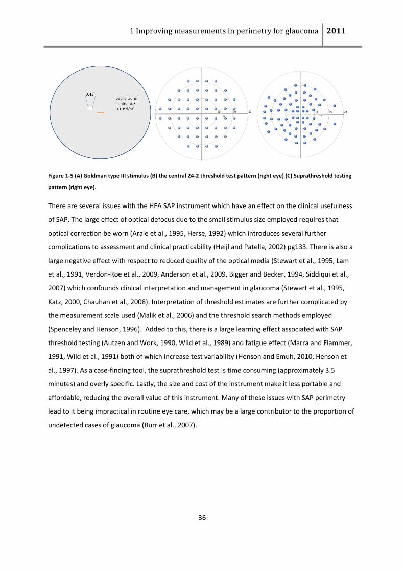
1 Improving measurements in perimetry for glaucoma 2011
36
Figure 1-5 (A) Goldman type III stimulus (B) the central 24-2 threshold test pattern (right eye) (C) Suprathreshold testing
pattern (right eye).
There are several issues with the HFA SAP instrument which have an effect on the clinical usefulness
of SAP. The large effect of optical defocus due to the small stimulus size employed requires that
optical correction be worn (Araie et al., 1995, Herse, 1992) which introduces several further
complications to assessment and clinical practicability (Heijl and Patella, 2002) pg133. There is also a
large negative effect with respect to reduced quality of the optical media (Stewart et al., 1995, Lam
et al., 1991, Verdon-Roe et al., 2009, Anderson et al., 2009, Bigger and Becker, 1994, Siddiqui et al.,
2007) which confounds clinical interpretation and management in glaucoma (Stewart et al., 1995,
Katz, 2000, Chauhan et al., 2008). Interpretation of threshold estimates are further complicated by
the measurement scale used (Malik et al., 2006) and the threshold search methods employed
(Spenceley and Henson, 1996). Added to this, there is a large learning effect associated with SAP
threshold testing (Autzen and Work, 1990, Wild et al., 1989) and fatigue effect (Marra and Flammer,
1991, Wild et al., 1991) both of which increase test variability (Henson and Emuh, 2010, Henson et
al., 1997). As a case-finding tool, the suprathreshold test is time consuming (approximately 3.5
minutes) and overly specific. Lastly, the size and cost of the instrument make it less portable and
affordable, reducing the overall value of this instrument. Many of these issues with SAP perimetry
lead to it being impractical in routine eye care, which may be a large contributor to the proportion of
undetected cases of glaucoma (Burr et al., 2007).
1 Improving measurements in perimetry for glaucoma 2011
37
1.7.3 Novel Perimetry
As previously discussed, structural loss is often observed at a retinal level before functional loss is
identified, and in particular of SAP, with the original white-on-white stimulus type and vice versa
(Quigley et al., 1982, Harwerth et al., 1999, Fraser and Manvikar, 2005). In an effort to detect
glaucoma earlier the search for newer perimetric techniques began. This was prompted by
histological studies undertaken in the late eighties and the early nineties (Glovinsky et al., 1993,
Quigley et al., 1987, Quigley et al., 1988), which suggested that in early glaucoma there may be
preferential damage to the M pathway (Weber et al., 2000, Chaturvedi et al., 1993). Recent work by
Yucel and colleagues has contradicted these findings, determining that no such preferential damage
occurs in glaucoma (Yücel et al., 2003, Ly et al., 2011, McKendrick et al., 2004). However, in the 20
year interim several new perimetric stimulus types were developed with the intention of exploiting
this phenomenon, mostly with stimulus types directed toward the M-pathway. While the
underpinning logic for development of the stimulus types has been eroded, potentially any of these
new perimetric instruments may offer improvements in value over the gold standard. This
improvement may manifest itself in simple things like the improvement of overall workflow of the
instrument, portability or affordability, or with a more stimulus based improvement such as
resilience to optical blur or media opacity or alternatively a simpler test may be more robust to
learning to fatigue effects. Here follows an overview of the some of these perimeters which are
commercially available or shortly will be.
1.7.3.1 Short Wavelength Automated Perimetry (SWAP)
SWAP has been implement within the HFA II, the stimulus is an intensity-modulated Goldman V blue
stimulus on a 100cd/m2 yellow background, presentation time is 200ms (Figure 1-6) (Johnson et al.,
1995). The standard test pattern remains the same as SAP, namely the 24-2 pattern (Figure 1-5 B).
Threshold is the lowest luminance at which the stimulus is detectable 50% of the times it is
presented. Similarly to SAP, the most used search method is SITA-Standard. Comparison in reliability
to full threshold has not been completed in the clinical instrument. SWAP has been shown to have
higher variability and there is a longer adaptation time than SAP (Moss et al., 1995). It has also been
shown to be more affected by lens opacity (Moss et al., 1995), and in particular with increases in
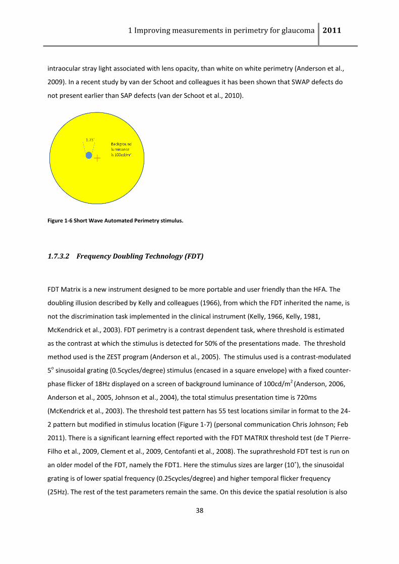
1 Improving measurements in perimetry for glaucoma 2011
38
intraocular stray light associated with lens opacity, than white on white perimetry (Anderson et al.,
2009). In a recent study by van der Schoot and colleagues it has been shown that SWAP defects do
not present earlier than SAP defects (van der Schoot et al., 2010).
Figure 1-6 Short Wave Automated Perimetry stimulus.
1.7.3.2 Frequency Doubling Technology (FDT)
FDT Matrix is a new instrument designed to be more portable and user friendly than the HFA. The
doubling illusion described by Kelly and colleagues (1966), from which the FDT inherited the name, is
not the discrimination task implemented in the clinical instrument (Kelly, 1966, Kelly, 1981,
McKendrick et al., 2003). FDT perimetry is a contrast dependent task, where threshold is estimated
as the contrast at which the stimulus is detected for 50% of the presentations made. The threshold
method used is the ZEST program (Anderson et al., 2005). The stimulus used is a contrast-modulated
5o sinusoidal grating (0.5cycles/degree) stimulus (encased in a square envelope) with a fixed counter-
phase flicker of 18Hz displayed on a screen of background luminance of 100cd/m2 (Anderson, 2006,
Anderson et al., 2005, Johnson et al., 2004), the total stimulus presentation time is 720ms
(McKendrick et al., 2003). The threshold test pattern has 55 test locations similar in format to the 24-
2 pattern but modified in stimulus location (Figure 1-7) (personal communication Chris Johnson; Feb
2011). There is a significant learning effect reported with the FDT MATRIX threshold test (de T Pierre-
Filho et al., 2009, Clement et al., 2009, Centofanti et al., 2008). The suprathreshold FDT test is run on
an older model of the FDT, namely the FDT1. Here the stimulus sizes are larger (10˚), the sinusoidal
grating is of lower spatial frequency (0.25cycles/degree) and higher temporal flicker frequency
(25Hz). The rest of the test parameters remain the same. On this device the spatial resolution is also
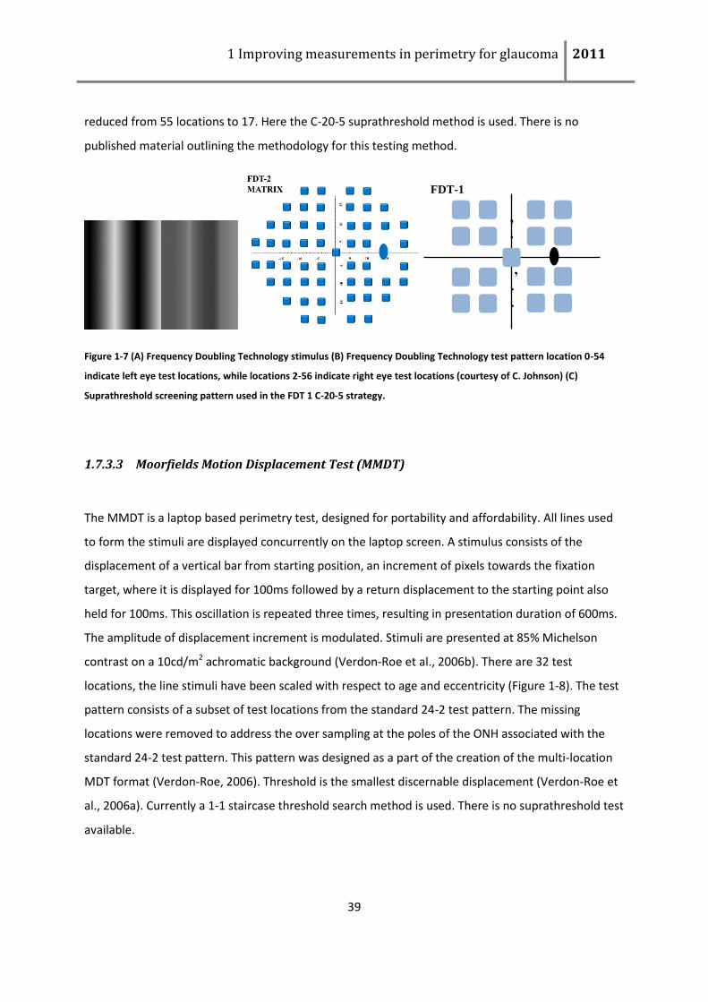
1 Improving measurements in perimetry for glaucoma 2011
39
reduced from 55 locations to 17. Here the C-20-5 suprathreshold method is used. There is no
published material outlining the methodology for this testing method.
Figure 1-7 (A) Frequency Doubling Technology stimulus (B) Frequency Doubling Technology test pattern location 0-54
indicate left eye test locations, while locations 2-56 indicate right eye test locations (courtesy of C. Johnson) (C)
Suprathreshold screening pattern used in the FDT 1 C-20-5 strategy.
1.7.3.3 Moorfields Motion Displacement Test (MMDT)
The MMDT is a laptop based perimetry test, designed for portability and affordability. All lines used
to form the stimuli are displayed concurrently on the laptop screen. A stimulus consists of the
displacement of a vertical bar from starting position, an increment of pixels towards the fixation
target, where it is displayed for 100ms followed by a return displacement to the starting point also
held for 100ms. This oscillation is repeated three times, resulting in presentation duration of 600ms.
The amplitude of displacement increment is modulated. Stimuli are presented at 85% Michelson
contrast on a 10cd/m2 achromatic background (Verdon-Roe et al., 2006b). There are 32 test
locations, the line stimuli have been scaled with respect to age and eccentricity (Figure 1-8). The test
pattern consists of a subset of test locations from the standard 24-2 test pattern. The missing
locations were removed to address the over sampling at the poles of the ONH associated with the
standard 24-2 test pattern. This pattern was designed as a part of the creation of the multi-location
MDT format (Verdon-Roe, 2006). Threshold is the smallest discernable displacement (Verdon-Roe et
al., 2006a). Currently a 1-1 staircase threshold search method is used. There is no suprathreshold test
available.
, . . .
. , . .
. . , .
.
-15
-10
-5
. . , .
. . . ,
. . . .
, . .
5
10
15
,
.
.
.
.
,
.
.
.
.
,
.
.
5
1
0
1
5
,
.
.
.
.
,
.
.
.
.
,
.
.
-
1
5
-
1
0
-
5
FDT-1
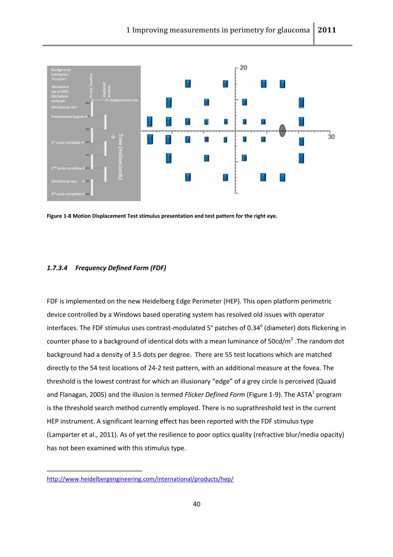
1 Improving measurements in perimetry for glaucoma 2011
40
Figure 1-8 Motion Displacement Test stimulus presentation and test pattern for the right eye.
1.7.3.4 Frequency Defined Form (FDF)
FDF is implemented on the new Heidelberg Edge Perimeter (HEP). This open platform perimetric
device controlled by a Windows based operating system has resolved old issues with operator
interfaces. The FDF stimulus uses contrast-modulated 5° patches of 0.34o (diameter) dots flickering in
counter phase to a background of identical dots with a mean luminance of 50cd/m2 .The random dot
background had a density of 3.5 dots per degree. There are 55 test locations which are matched
directly to the 54 test locations of 24-2 test pattern, with an additional measure at the fovea. The
threshold is the lowest contrast for which an illusionary “edge” of a grey circle is perceived (Quaid
and Flanagan, 2005) and the illusion is termed Flicker Defined Form (Figure 1-9). The ASTA1 program
is the threshold search method currently employed. There is no suprathreshold test in the current
HEP instrument. A significant learning effect has been reported with the FDF stimulus type
(Lamparter et al., 2011). As of yet the resilience to poor optics quality (refractive blur/media opacity)
has not been examined with this stimulus type.
http://www.heidelbergengineering.com/international/products/hep/
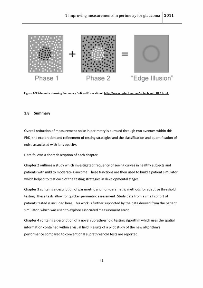
1 Improving measurements in perimetry for glaucoma 2011
41
Figure 1-9 Schematic showing Frequency Defined Form stimuli http://www.optech.net.au/optech_net_HEP.html.
1.8 Summary
Overall reduction of measurement noise in perimetry is pursued through two avenues within this
PhD, the exploration and refinement of testing strategies and the classification and quantification of
noise associated with lens opacity.
Here follows a short description of each chapter.
Chapter 2 outlines a study which investigated frequency of seeing curves in healthy subjects and
patients with mild to moderate glaucoma. These functions are then used to build a patient simulator
which helped to test each of the testing strategies in developmental stages.
Chapter 3 contains a description of parametric and non-parametric methods for adaptive threshold
testing. These tests allow for quicker perimetric assessment. Study data from a small cohort of
patients tested is included here. This work is further supported by the data derived from the patient
simulator, which was used to explore associated measurement error.
Chapter 4 contains a description of a novel suprathreshold testing algorithm which uses the spatial
information contained within a visual field. Results of a pilot study of the new algorithm’s
performance compared to conventional suprathreshold tests are reported.

1 Improving measurements in perimetry for glaucoma 2011
42
Chapter 5 describes studies that have used the test methods developed in the preceding chapters
and provides evidence for their utility and comparable performance with other perimetric methods
and devices.
Chapter 6 presents a study which investigates perimetric measurement error associated with lens
opacity. Lens opacity induces an increase in intraocular stray light, which in conventional perimetry is
often perceived as a lowering of the retinal sensitivity. In perimetric measures this is a major
confounder to correct interpretation. In this study the level of intraocular stray light is systematically
increased in visually healthy observers to examine the effect on retinal sensitivity measures.
Chapter 7 summaries the main findings from the work described in this thesis and offers some future
projects associated with the work.
2 Frequency of seeing and the observer response simulator
The work described in this chapter leads to the development of an observer response simulator
(ORS). This ORS was used to test potential testing strategies in chapter 3. The results in this chapter
have been presented, in part, as a read paper at the 18th International Symposium of the Imaging and
Perimetry Society Meeting in Nara, Japan in May 2008 (See ‘List of supporting publications’). Data
collected in this study were collected by CB and Reza Moosavi MD at Moorfields Eye Hospital.
In chapter 1 the sources of measurement noise with instruments in glaucoma diagnosis and
monitoring were discussed, in particular those associated with perimetric measures. Measurement
noise in perimetry may be due to the testing algorithm or other factors, for example, where retinal
sensitivity was underestimated due to the reduced quality of the optics. However, the most
convoluted source of measurement noise in perimetry originates from the subjective nature of the
test (dependence on observer response). In this case the false positive (FP) (or guess) rate and false
negative (FN) (or lapse) rate will significantly influence the test results, as will the response
confidence of the observer (Wichmann and Hill, 2001a) (Figure 2-1). FP rate is the proportion of
responses which were unseen but the observer provided a seen response. This is sometimes referred
to as ‘trigger happiness’. FN rate is the proportion of responses which were easily visible but the
observer provided an unseen response or in lapse in concentration. High confidence of an observer
in comparison to an observer with lower confidence (even with matching sensitivity), would equate
to a smaller interval of intensities which cover the range from where the stimulus is easily visible to
where it is not visible.
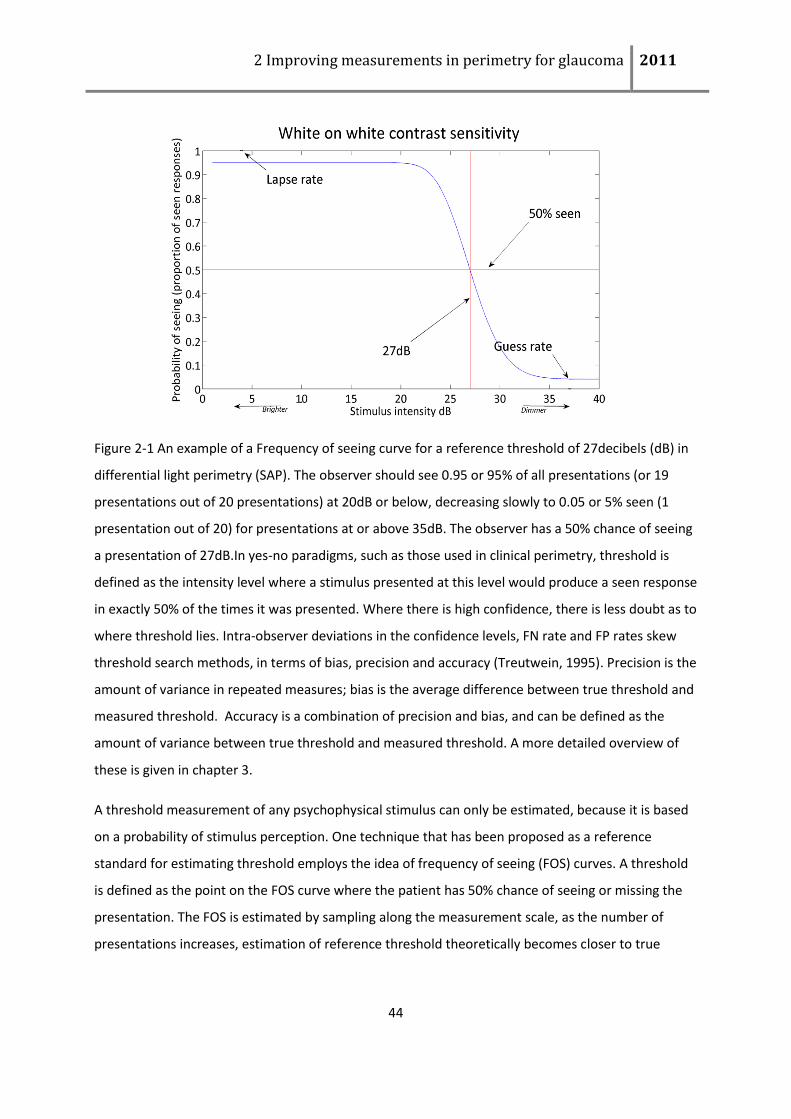
2 Improving measurements in perimetry for glaucoma 2011
44
Figure 2-1 An example of a Frequency of seeing curve for a reference threshold of 27decibels (dB) in
differential light perimetry (SAP). The observer should see 0.95 or 95% of all presentations (or 19
presentations out of 20 presentations) at 20dB or below, decreasing slowly to 0.05 or 5% seen (1
presentation out of 20) for presentations at or above 35dB. The observer has a 50% chance of seeing
a presentation of 27dB.In yes-no paradigms, such as those used in clinical perimetry, threshold is
defined as the intensity level where a stimulus presented at this level would produce a seen response
in exactly 50% of the times it was presented. Where there is high confidence, there is less doubt as to
where threshold lies. Intra-observer deviations in the confidence levels, FN rate and FP rates skew
threshold search methods, in terms of bias, precision and accuracy (Treutwein, 1995). Precision is the
amount of variance in repeated measures; bias is the average difference between true threshold and
measured threshold. Accuracy is a combination of precision and bias, and can be defined as the
amount of variance between true threshold and measured threshold. A more detailed overview of
these is given in chapter 3.
A threshold measurement of any psychophysical stimulus can only be estimated, because it is based
on a probability of stimulus perception. One technique that has been proposed as a reference
standard for estimating threshold employs the idea of frequency of seeing (FOS) curves. A threshold
is defined as the point on the FOS curve where the patient has 50% chance of seeing or missing the
presentation. The FOS is estimated by sampling along the measurement scale, as the number of
presentations increases, estimation of reference threshold theoretically becomes closer to true
2 Improving measurements in perimetry for glaucoma 2011
45
threshold. The slope of the FOS curve can be interpreted as the amount of ‘doubt’ around threshold
or confidence of the observer and therefore is directly related to precision.
FOS curves are designed to describe the signal strength required by an observer to accomplish a
given perceptual task. The method of constant stimuli (MOCS) refers to the data collection procedure
where an equivalent number of presentations are displayed at each intensity level and the order of
displaying intensity levels is randomised. These data are then used to construct the associated
frequency of seeing curve (Wichmann and Hill, 2001a, Treutwein and Strasburger, 1999). Despite
being time consuming (Watson and Fitzhugh, 1990), MOCS is a standard method in psychophysics
(Treutwein, 1995) for collecting FOS data.
In clinical perimetry, full VF assessment takes from about 4 to 7 minutes per eye for 24-2 SITA
standard but can take up to 15 minutes per eye for a full threshold 30-2 test. FOS data collection
requires anything between 40-120+ presentations per location depending on the level of precision
required and can last as long as 70 minutes for adaptive FOS at 52 locations (estimate using method
described by Turpin (Turpin et al., 2010)). This type of FOS data collection is clearly not feasible in the
clinical setting. Yet it is accepted that the estimated threshold measures from FOS data collection are
superior (have greater accuracy) to those estimated using clinical search methods (Turpin et al.,
2000, Treutwein, 1995). When threshold is calculated from constructed FOS curves it is generally
referred to as “reference” threshold (Treutwein, 1995).
With the ‘ideal’ visually healthy observer, systematic bias in measures should only be expected to
vary with eccentricity or with age. It has been shown that threshold and slope of the FOS curve will
vary between locations in healthy observers (Wall et al., 1996, Henson et al., 2000, Spry et al., 2001,
Gilmore et al., 2005, Verdon-Roe et al., 2006a, Olsson et al., 1993, Westcott et al., 1999): central
locations will have higher sensitivity presented by upward shifted FOS curves with steep slopes (Wall
et al., 1996). As the degree the stimulus is subtended from the fixation point (or eccentricity)
increases, the FOS curve experiences a downward shift (lowering of sensitivity) in threshold and a
decrease in slope.
The shape and position of the curve also vary between subjects, especially with respect to age or
glaucomatous field damage (Henson et al., 2000). In damaged test locations the shift will be
significantly greater than that expected with age alone (Henson et al., 2000, Chauhan et al., 1993,
Westcott et al., 1999). Thus to be able to simulate observer responses throughout the field, FOS data
2 Improving measurements in perimetry for glaucoma 2011
46
should ideally be collected at a range of eccentricities and subjects presenting with a whole spectrum
of disease stages and a wide age range.
By using FOS curves it is possible to estimate bias and precision of clinical threshold search methods
in two ways. Firstly, by constructing FOS curves and deriving a “reference threshold” in a cohort of
subjects, then comparing this to threshold measures yielded from clinical search methods collected
directly from the same cohort. Secondly by computer simulation; in this case the clinical search
method utilises simulated observer responses from the underlying probability function of the
respective FOS curve. The latter can be used to generate a series of ‘patient’ trials with each clinical
search method, returning a distribution of possible threshold values. Bias and precision can be
estimated from these data.
2.1 Observer response simulator
The aim of the work described in this chapter is to implement a series of FOS experiments to be used
in the development of an observer response simulator (ORS). This in turn will be used as a reference
standard and test-bed for the perimetry strategies developed in subsequent chapters. Simply put, an
ORS uses the FOS curve to assign a probability to how a given observer would respond to a given
“event” or stimulus presentation. An ORS acts like a ‘robot’ observer. Variants of this method were
previously described (Swanson and Birch, 1992, Spenceley and Henson, 1996) to assess variability.
Artes and colleagues used this approach (Artes et al., 2002a) to assess the comparative performance
of clinical suprathreshold methodologies and Turpin and colleagues (Turpin et al., 2002a) to assess
the comparative performance of the perimetric clinical threshold search methods. In the subsequent
chapters this patient simulated approach of assessing clinical perimetric testing methods will be
utilized to obtain relevant comparative threshold search data and comparative suprathreshold data.
The ORS is the simple idea of selecting a random value from a uniform distribution between 0 and 1.
Then a presentation response is simulated by ORS with the logical question, ‘is this random value
below the FOS curve at this presentation intensity level?’ If the answer is yes, then a seen response is
recorded. Otherwise an unseen response is recorded. For example, if the presentation is set at an
intensity which equates to an 88% probability of being seen (e.g. Figure 2-2, 4 pixel movement), then
the ORS will return a seen answer for on average 88/100 trials simulated.
2 Improving measurements in perimetry for glaucoma 2011
47
If an ORS is working in conjunction with a clinical threshold search method, then the stimulus
intensity is going to change as the search progresses. In the example illustrated in Figure 2-1 if a seen
response was returned after a presentation was made at a 28dB, then there will be a upwards shift in
sensitivity values (reduction in stimulus intensity) to 30dB for the subsequent presentation. At this
point the ORS assigns a 17% probability to seen response. In this way the ORS will give appropriate
answers at each stage.
By assessing clinical search methods with responses generated from ORS, it is possible to compile a
large set of trials. Each threshold testing strategy can be assessed in terms of accuracy, bias and
precision without requiring the test subject to return multiple times. Repeating the experiment
under variants of various parameters, including for example step size, starting point and termination
criteria, then the usefulness of this methodology quickly becomes apparent. Results are then used to
compare accuracy, bias and precision with respect to many variants of each clinical search method.
In this manner the most efficient parameters for each clinical search method can be found. This
methodology has been used previously by Turpin and colleagues for the development of testing
strategies for the FDT (Turpin et al., 2002a, Turpin et al., 2003).
2.2 Frequency of seeing: methods and modelling
FOS data has been collected in glaucomatous patients using the MMDT stimulus type once previously
(Westcott et al., 1998), but the test has had marked changes in screen, viewing distance, stimulus
and format. Previously a monochromatic monitor (Phillips green monochrome P31 monitor, model
number 750205, pixilation 300x920, frame rate 50 Hz) was used. In this new experiment a LCD screen
was used (Lenovo: Thinkpad W500, resolution 1920x1200 pixels, frame refresh rate of 60Hz).
Previously the viewing distance was 1.24 m (resulting in a minimum angle subtended of 1.1 minutes
of arc (+15⁰,+09⁰)), currently the test is performed at 30cm (resulting in a minimum angle subtended
of 1.8 minutes of arc (+15⁰,+09⁰)). On the original MMDT test instrument the stimulus size subtended
2.2 minutes of arc, however with the multi-location MMDT format the stimuli are scaled with ages
and eccentricity and so vary in size. Stimuli in the previous study had a background luminance of 7
cd/m2 and the stimulus luminance was 27 cd/m2. In this new experiment the background is on
average 10 cd/m2 (varying from 6cd/m2 to 14cd/m2 due to angular luminance) with a stimulus of
2 Improving measurements in perimetry for glaucoma 2011
48
105cd/m2 (varying between 100cd/m2 to 112 cd/m2). Michelson contrast is maintained at between
80% and 90% for all locations.
The primary aim of the study described in this chapter was to collect FOS type data on the new
MMDT stimuli in a group of glaucomatous patients and visually healthy subjects across a range of
eccentricities to develop an ORS for MMDT stimuli. This has not been done before. This ORS will be
used to assess the performance of the clinical threshold search methods for the MMDT invented in
subsequent chapters.
MOCS method was also used for the data collection within this study; however, some minor
modifications have been made. At each test location an effort was made to assess at least the 5% to
95% segment of the FOS curve of the MMDT stimulus type (section 1.4.3) as it was shown to be a
sampling scheme with less bias and better precision than alternative schemes (Wichmann and Hill,
2001a).
An important restriction with the MMDT stimulus type, left unexpanded until this point, is pixel pitch.
With MMDT the stimulus intensity is displacement size, the possible range of which is restricted by
the pixel pitch of the monitor used. (Up until this point a Dell monitor of pixel pitch 0.26mm was
used). In DLS the contrast can be reduced until the background and foreground are inseparable in all
observers. Unlike DLS where intensity levels are log units, the intensity levels of the MMDT are
minutes of arc subtended. With the MMDT, the minimum possible movement in some young
observers remains apparent, which means the lower end of the FOS curve is lower than that which is
measureable. An example of the pixel pitch dividing the FOS curve is shown in Figure 2-2 with the
green vertical lines (2.4 minutes of arc apart) representing the minimum step size available.
A further complication with working on a scale depending on pixel pitch and minutes of arc is the
inconsistency in intensity levels across the field. Pixel pitch is consistent across the screen, however
as eccentricity increases, the distance from the eye to the screen increases and as a consequence the
angle subtended decreases. Therefore, while a displacement of 9 pixels subtends 25.7 MoA at a
location positioned 3 degrees temporally and 3 degrees inferiorly (+3⁰,-3⁰), the same displacement of
9 pixels will subtend 20.5MoA at a location 27 degrees nasally and 3 degrees superiorly (-27⁰,+3⁰).
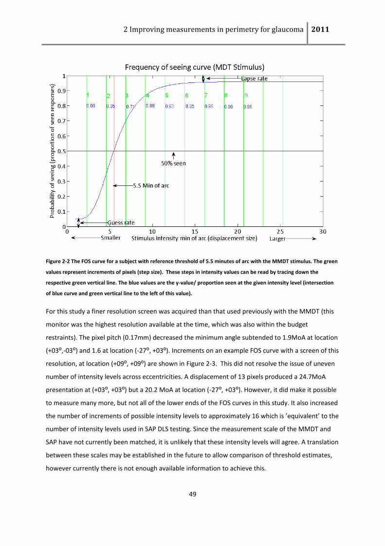
2 Improving measurements in perimetry for glaucoma 2011
49
Figure 2-2 The FOS curve for a subject with reference threshold of 5.5 minutes of arc with the MMDT stimulus. The green
values represent increments of pixels (step size). These steps in intensity values can be read by tracing down the
respective green vertical line. The blue values are the y-value/ proportion seen at the given intensity level (intersection
of blue curve and green vertical line to the left of this value).
For this study a finer resolution screen was acquired than that used previously with the MMDT (this
monitor was the highest resolution available at the time, which was also within the budget
restraints). The pixel pitch (0.17mm) decreased the minimum angle subtended to 1.9MoA at location
(+03⁰,-03⁰) and 1.6 at location (-27⁰, +03⁰). Increments on an example FOS curve with a screen of this
resolution, at location (+09⁰, +09⁰) are shown in Figure 2-3. This did not resolve the issue of uneven
number of intensity levels across eccentricities. A displacement of 13 pixels produced a 24.7MoA
presentation at (+03⁰, +03⁰) but a 20.2 MoA at location (-27⁰, +03⁰). However, it did make it possible
to measure many more, but not all of the lower ends of the FOS curves in this study. It also increased
the number of increments of possible intensity levels to approximately 16 which is ’equivalent’ to the
number of intensity levels used in SAP DLS testing. Since the measurement scale of the MMDT and
SAP have not currently been matched, it is unlikely that these intensity levels will agree. A translation
between these scales may be established in the future to allow comparison of threshold estimates,
however currently there is not enough available information to achieve this.
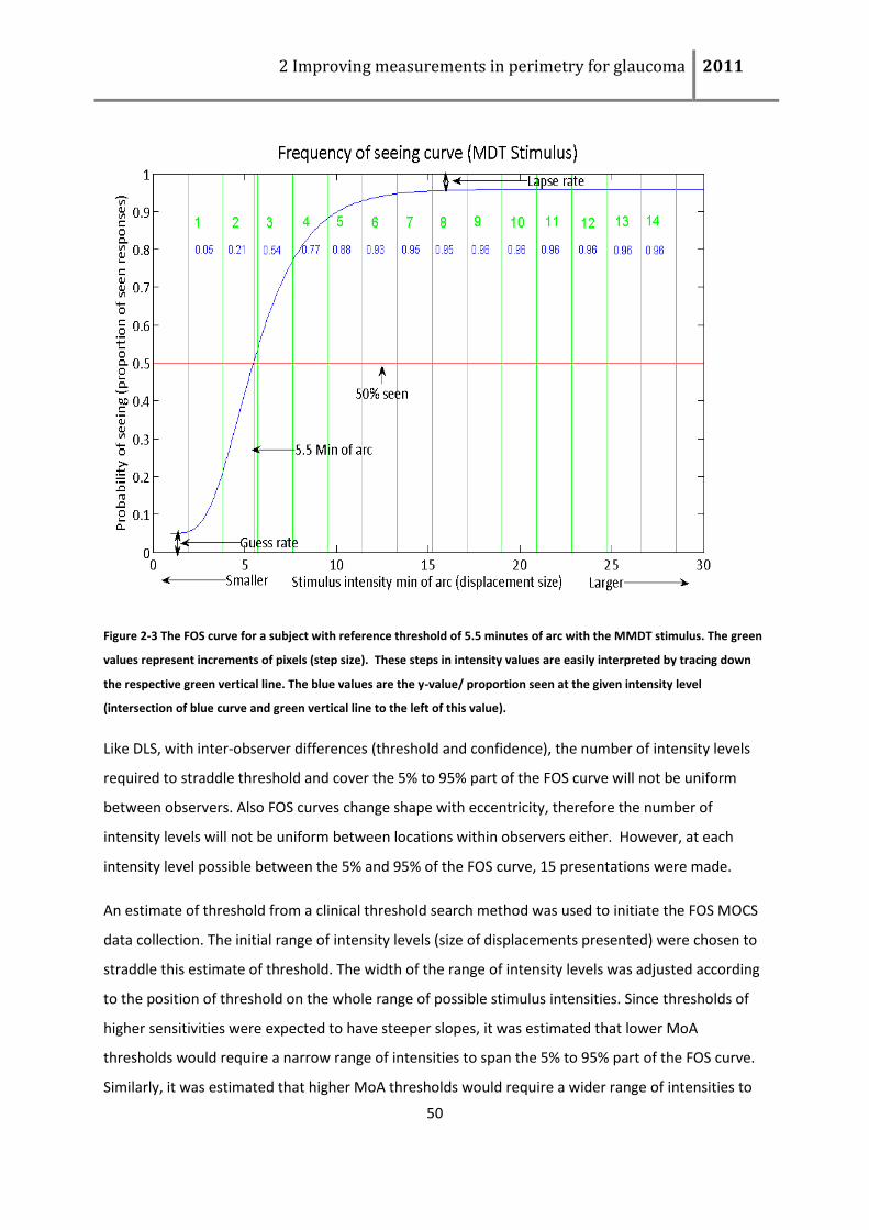
2 Improving measurements in perimetry for glaucoma 2011
50
Figure 2-3 The FOS curve for a subject with reference threshold of 5.5 minutes of arc with the MMDT stimulus. The green
values represent increments of pixels (step size). These steps in intensity values are easily interpreted by tracing down
the respective green vertical line. The blue values are the y-value/ proportion seen at the given intensity level
(intersection of blue curve and green vertical line to the left of this value).
Like DLS, with inter-observer differences (threshold and confidence), the number of intensity levels
required to straddle threshold and cover the 5% to 95% part of the FOS curve will not be uniform
between observers. Also FOS curves change shape with eccentricity, therefore the number of
intensity levels will not be uniform between locations within observers either. However, at each
intensity level possible between the 5% and 95% of the FOS curve, 15 presentations were made.
An estimate of threshold from a clinical threshold search method was used to initiate the FOS MOCS
data collection. The initial range of intensity levels (size of displacements presented) were chosen to
straddle this estimate of threshold. The width of the range of intensity levels was adjusted according
to the position of threshold on the whole range of possible stimulus intensities. Since thresholds of
higher sensitivities were expected to have steeper slopes, it was estimated that lower MoA
thresholds would require a narrow range of intensities to span the 5% to 95% part of the FOS curve.
Similarly, it was estimated that higher MoA thresholds would require a wider range of intensities to
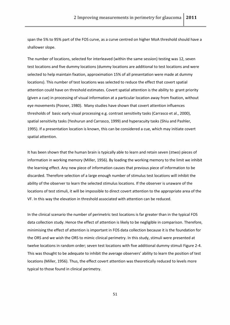
2 Improving measurements in perimetry for glaucoma 2011
51
span the 5% to 95% part of the FOS curve, as a curve centred on higher MoA threshold should have a
shallower slope.
The number of locations, selected for interleaved (within the same session) testing was 12, seven
test locations and five dummy locations (dummy locations are additional to test locations and were
selected to help maintain fixation, approximation 15% of all presentation were made at dummy
locations). This number of test locations was selected to reduce the effect that covert spatial
attention could have on threshold estimates. Covert spatial attention is the ability to grant priority
(given a cue) in processing of visual information at a particular location away from fixation, without
eye movements (Posner, 1980). Many studies have shown that covert attention influences
thresholds of basic early visual processing e.g. contrast sensitivity tasks (Carrasco et al., 2000),
spatial sensitivity tasks (Yeshurun and Carrasco, 1999) and hyperacuity tasks (Shiu and Pashler,
1995). If a presentation location is known, this can be considered a cue, which may initiate covert
spatial attention.
It has been shown that the human brain is typically able to learn and retain seven (±two) pieces of
information in working memory (Miller, 1956). By loading the working memory to the limit we inhibit
the learning effect. Any new piece of information causes that previous piece of information to be
discarded. Therefore selection of a large enough number of stimulus test locations will inhibit the
ability of the observer to learn the selected stimulus locations. If the observer is unaware of the
locations of test stimuli, it will be impossible to direct covert attention to the appropriate area of the
VF. In this way the elevation in threshold associated with attention can be reduced.
In the clinical scenario the number of perimetric test locations is far greater than in the typical FOS
data collection study. Hence the effect of attention is likely to be negligible in comparison. Therefore,
minimising the effect of attention is important in FOS data collection because it is the foundation for
the ORS and we wish the ORS to mimic clinical perimetry. In this study, stimuli were presented at
twelve locations in random order; seven test locations with five additional dummy stimuli Figure 2-4.
This was thought to be adequate to inhibit the average observers’ ability to learn the position of test
locations (Miller, 1956). Thus, the effect covert attention was theoretically reduced to levels more
typical to those found in clinical perimetry.
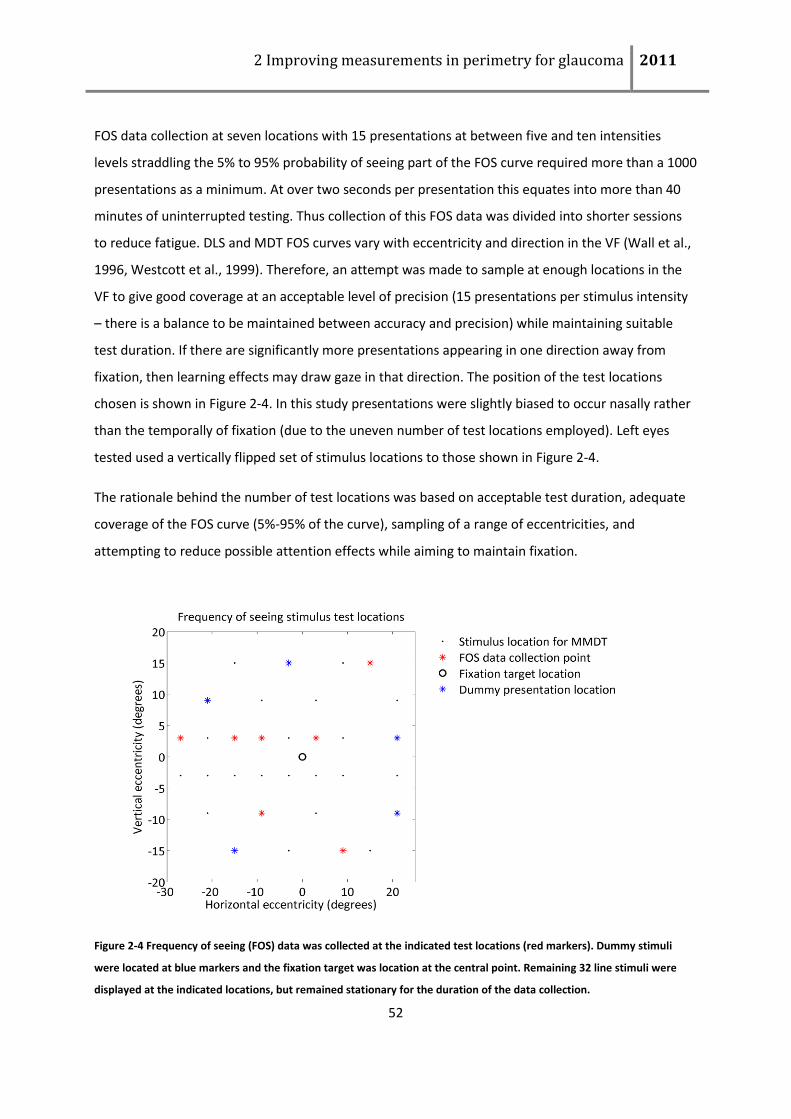
2 Improving measurements in perimetry for glaucoma 2011
52
FOS data collection at seven locations with 15 presentations at between five and ten intensities
levels straddling the 5% to 95% probability of seeing part of the FOS curve required more than a 1000
presentations as a minimum. At over two seconds per presentation this equates into more than 40
minutes of uninterrupted testing. Thus collection of this FOS data was divided into shorter sessions
to reduce fatigue. DLS and MDT FOS curves vary with eccentricity and direction in the VF (Wall et al.,
1996, Westcott et al., 1999). Therefore, an attempt was made to sample at enough locations in the
VF to give good coverage at an acceptable level of precision (15 presentations per stimulus intensity
– there is a balance to be maintained between accuracy and precision) while maintaining suitable
test duration. If there are significantly more presentations appearing in one direction away from
fixation, then learning effects may draw gaze in that direction. The position of the test locations
chosen is shown in Figure 2-4. In this study presentations were slightly biased to occur nasally rather
than the temporally of fixation (due to the uneven number of test locations employed). Left eyes
tested used a vertically flipped set of stimulus locations to those shown in Figure 2-4.
The rationale behind the number of test locations was based on acceptable test duration, adequate
coverage of the FOS curve (5%-95% of the curve), sampling of a range of eccentricities, and
attempting to reduce possible attention effects while aiming to maintain fixation.
Figure 2-4 Frequency of seeing (FOS) data was collected at the indicated test locations (red markers). Dummy stimuli
were located at blue markers and the fixation target was location at the central point. Remaining 32 line stimuli were
displayed at the indicated locations, but remained stationary for the duration of the data collection.
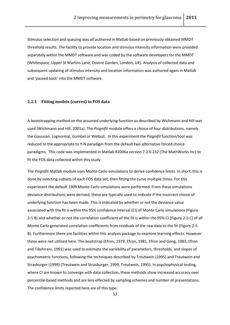
2 Improving measurements in perimetry for glaucoma 2011
53
Stimulus selection and queuing was all authored in Matlab based on previously obtained MMDT
threshold results. The facility to provide location and stimulus intensity information were provided
separately within the MMDT software and was coded by the software developers for the MMDT
(Whitespace, Upper St Martins Lane, Covent Garden, London, UK). Analysis of collected data and
subsequent updating of stimulus intensity and location information was authored again in Matlab
and ‘passed back’ into the MMDT software.
2.2.1 Fitting models (curves) to FOS data
A bootstrapping method on the assumed underlying function as described by Wichmann and Hill was
used (Wichmann and Hill, 2001a). The Psignifit module offers a choice of four distributions, namely
the Gaussian, Lognormal, Gumbel or Weibull. In this experiment the Psignifit function/tool was
reduced to the appropriate to Y-N paradigm from the default two alternative forced choice
paradigms. This code was implemented in Matlab R2006a version 7.2.0.232 (The MathWorks Inc) to
fit the FOS data collected within this study.
The Psignifit Matlab module uses Monte Carlo simulations to derive confidence limits. In short, this is
done by selecting subsets of each FOS data set, then fitting the curve multiple times. For this
experiment the default 1999 Monte Carlo simulations were performed. From these simulations
deviance distributions were derived; these are typically used to indicate if the incorrect choice of
underlying function has been made. This is indicated by whether or not the deviance value
associated with the fit is within the 95% confidence interval (CI) of Monte Carlo simulations (Figure
2-5 B) and whether or not the correlation coefficient of the fit is within the 95% CI (Figure 2-5 C) of all
Monte Carlo generated correlation coefficients from residuals of the raw data to the fit (Figure 2-5
B). Furthermore there are facilities within this analysis package to examine learning effects. However
these were not utilised here. The bootstrap (Efron, 1979, Efron, 1981, Efron and Gong, 1983, Efron
and Tibshirani, 1991) was used to estimate the variability of parameters, thresholds, and slopes of
psychometric functions, following the techniques described by Treutwein (1995) and Treutwein and
Strasburger (1999) (Treutwein and Strasburger, 1999, Treutwein, 1995). In psychophysical testing,
where CI are known to converge with data collection, these methods show increased accuracy over
percentile-based methods and are less effected by sampling schemes and number of presentations.
The confidence limits reported here are of this type.
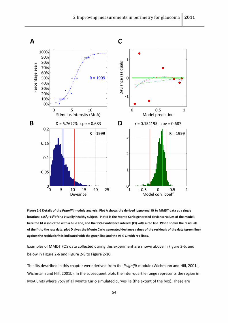
2 Improving measurements in perimetry for glaucoma 2011
54
Figure 2-5 Details of the Psignifit module analysis. Plot A shows the derived lognormal fit to MMDT data at a single
location (+15⁰,+15⁰) for a visually healthy subject. Plot B is the Monte Carlo generated deviance values of the model;
here the fit is indicated with a blue line, and the 95% Confidence interval (CI) with a red line. Plot C shows the residuals
of the fit to the raw data, plot D gives the Monte Carlo generated deviance values of the residuals of the data (green line)
against the residuals fit is indicated with the green line and the 95% CI with red lines.
Examples of MMDT FOS data collected during this experiment are shown above in Figure 2-5, and
below in Figure 2-6 and Figure 2-8 to Figure 2-10.
The fits described in this chapter were derived from the Psignifit module (Wichmann and Hill, 2001a,
Wichmann and Hill, 2001b). In the subsequent plots the inter-quartile range represents the region in
MoA units where 75% of all Monte Carlo simulated curves lie (the extent of the box). These are
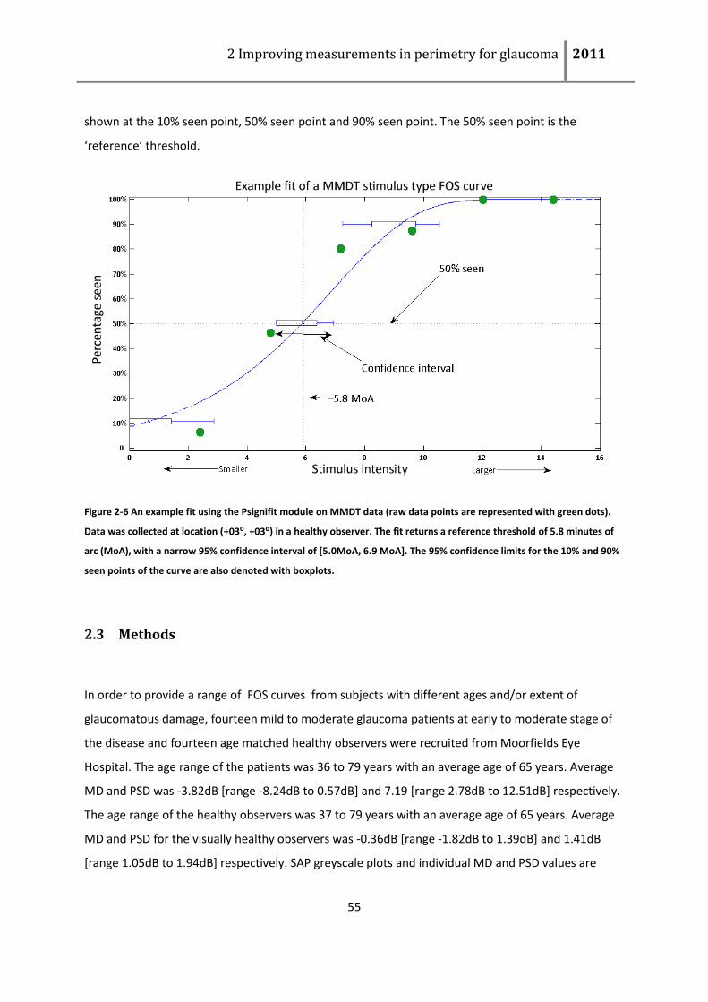
2 Improving measurements in perimetry for glaucoma 2011
55
shown at the 10% seen point, 50% seen point and 90% seen point. The 50% seen point is the
‘reference’ threshold.
Figure 2-6 An example fit using the Psignifit module on MMDT data (raw data points are represented with green dots).
Data was collected at location (+03⁰, +03⁰) in a healthy observer. The fit returns a reference threshold of 5.8 minutes of
arc (MoA), with a narrow 95% confidence interval of [5.0MoA, 6.9 MoA]. The 95% confidence limits for the 10% and 90%
seen points of the curve are also denoted with boxplots.
2.3 Methods
In order to provide a range of FOS curves from subjects with different ages and/or extent of
glaucomatous damage, fourteen mild to moderate glaucoma patients at early to moderate stage of
the disease and fourteen age matched healthy observers were recruited from Moorfields Eye
Hospital. The age range of the patients was 36 to 79 years with an average age of 65 years. Average
MD and PSD was -3.82dB [range -8.24dB to 0.57dB] and 7.19 [range 2.78dB to 12.51dB] respectively.
The age range of the healthy observers was 37 to 79 years with an average age of 65 years. Average
MD and PSD for the visually healthy observers was -0.36dB [range -1.82dB to 1.39dB] and 1.41dB
[range 1.05dB to 1.94dB] respectively. SAP greyscale plots and individual MD and PSD values are
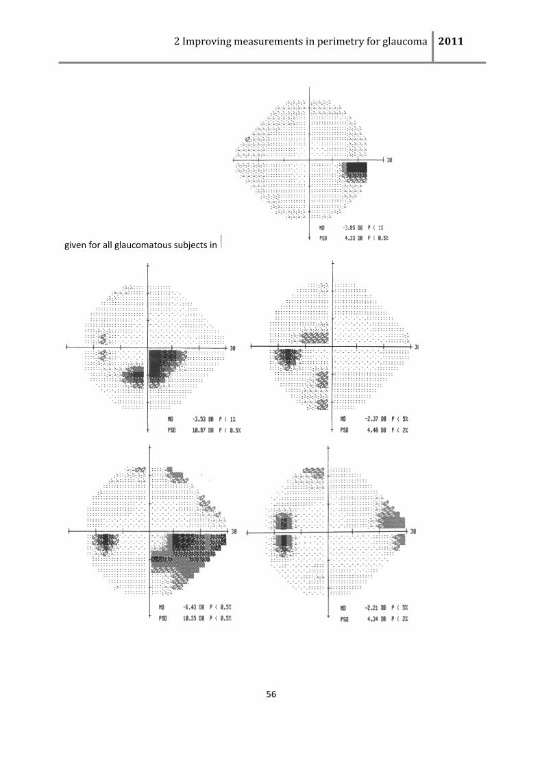
2 Improving measurements in perimetry for glaucoma 2011
56
given for all glaucomatous subjects in

2 Improving measurements in perimetry for glaucoma 2011
57
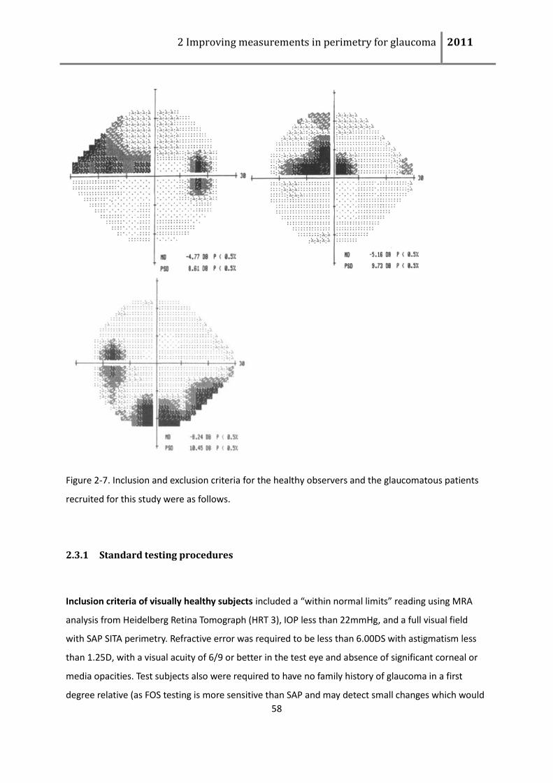
2 Improving measurements in perimetry for glaucoma 2011
58
Figure 2-7. Inclusion and exclusion criteria for the healthy observers and the glaucomatous patients
recruited for this study were as follows.
2.3.1 Standard testing procedures
Inclusion criteria of visually healthy subjects included a “within normal limits” reading using MRA
analysis from Heidelberg Retina Tomograph (HRT 3), IOP less than 22mmHg, and a full visual field
with SAP SITA perimetry. Refractive error was required to be less than 6.00DS with astigmatism less
than 1.25D, with a visual acuity of 6/9 or better in the test eye and absence of significant corneal or
media opacities. Test subjects also were required to have no family history of glaucoma in a first
degree relative (as FOS testing is more sensitive than SAP and may detect small changes which would
2 Improving measurements in perimetry for glaucoma 2011
59
be undetectable with SAP) or ocular/systemic disease which is likely to affect visual performance (e.g.
diabetes, thyroid disease). No history of previous ocular surgery (apart from uncomplicated cataract).
Inclusion criteria of glaucomatous patients included an “outside normal limits” reading using MRA
analysis from Heidelberg Retina Tomograph (HRT 3), IOP greater than 21mmHg before treatment, a
full visual field with SAP SITA perimetry, and a gonioscopically open angle. Refractive error was
required to be less than 6.00DS with astigmatism less than 1.25D, with a visual acuity of 6/12 or
better in the test eye and absence of significant corneal or media opacities. Exclusion criteria were
secondary causes of elevated IOP, other than pseudoexfoliation and pigment dispersion. No history of
diabetic retinopathy or previous retinal vein occlusion or history of ocular surgery, previous stroke,
ocular trauma or amblyopia. No history of previous ocular surgery (apart from uncomplicated
cataract).
All participant testing for this thesis was done at Moorfields Eye Hospital by CB and by Reza Moosavi
[RM] MD. The study was approved by an ethics committee and conformed to the Declaration of
Helsinki with all participants giving their informed written consent. All data was anonymised before
being transferred to a secure computer database at the university. Data was collected at all seven
test locations in the visually healthy subjects. In glaucomatous patients, data was collected at
corresponding test locations with early to moderate visual field damage, but test locations which fell
within deep focal defects were excluded from data collection. Presentations were made at a
minimum of 9 test locations in all subjects. The number of sessions varied between subjects
(between six and twelve sessions) due to the width of the range of intensities tested and number of
locations where data collection was possible. There was an extended break after every three
sessions. No test session was greater than 7 minutes long. Observers could take a break at any stage.
During session breaks, the probability of seeing at the chosen intensity levels was calculated. This
information was then used to review the interim FOS curve. If it was determined that the 5% to the
95% range of the FOS curve was not within the range of test intensities levels, then the range was
expanded to accommodate These (with new bins added).
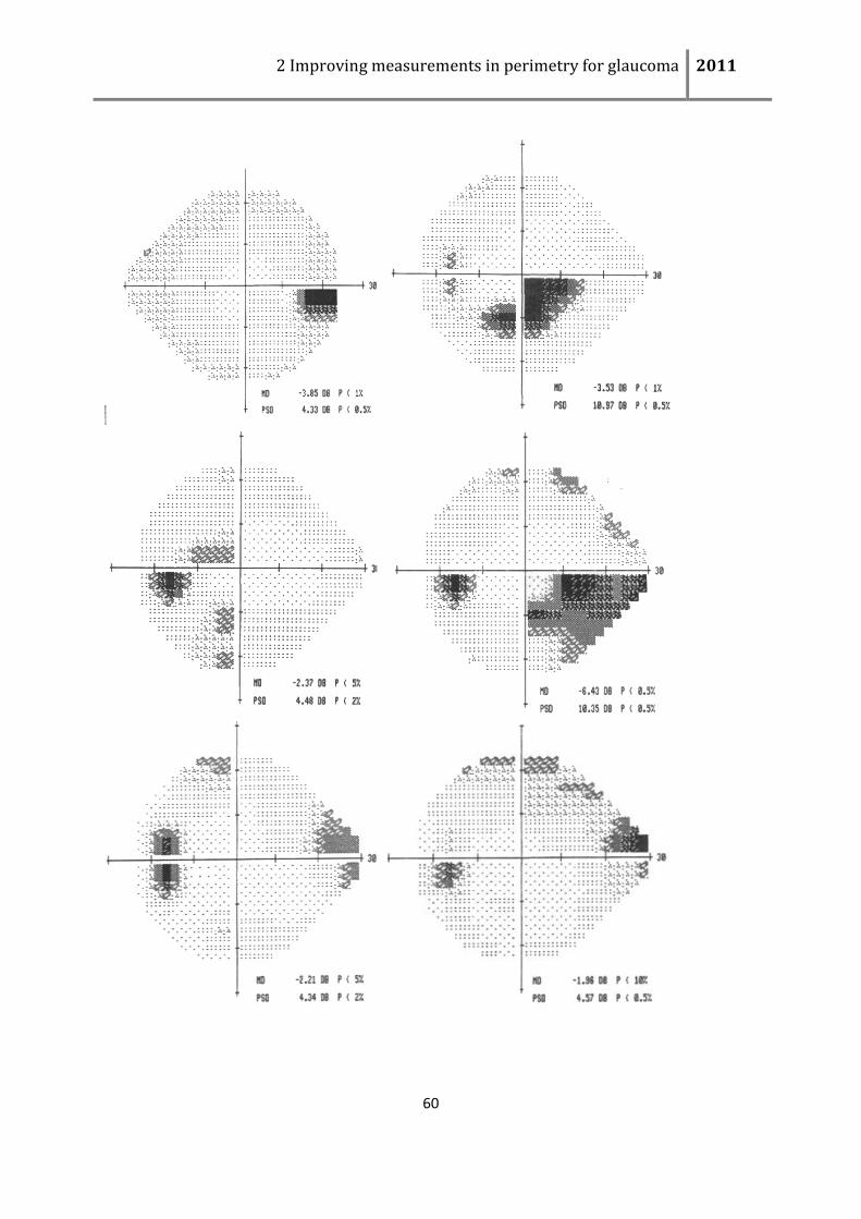
2 Improving measurements in perimetry for glaucoma 2011
60
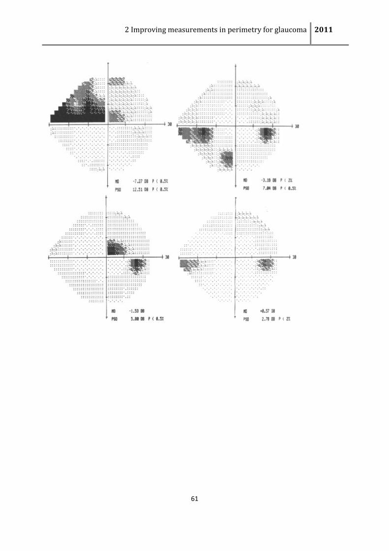
2 Improving measurements in perimetry for glaucoma 2011
61
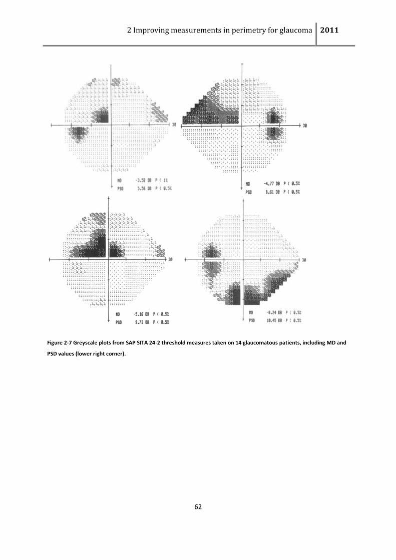
2 Improving measurements in perimetry for glaucoma 2011
62
Figure 2-7 Greyscale plots from SAP SITA 24-2 threshold measures taken on 14 glaucomatous patients, including MD and
PSD values (lower right corner).
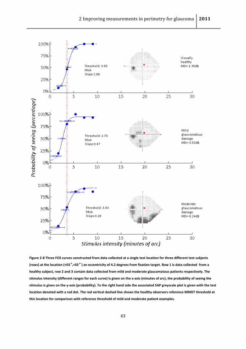
2 Improving measurements in perimetry for glaucoma 2011
63
Figure 2-8 Three FOS curves constructed from data collected at a single test location for three different test subjects
(rows) at the location (+03 o
,+03 o
) an eccentricity of 4.2 degrees from fixation target. Row 1 is data collected from a
healthy subject, row 2 and 3 contain data collected from mild and moderate glaucomatous patients respectively. The
stimulus intensity (different ranges for each curve) is given on the x-axis (minutes of arc), the probability of seeing the
stimulus is given on the y-axis (probability). To the right hand side the associated SAP greyscale plot is given with the test
location denoted with a red dot. The red vertical dashed line shows the healthy observers reference MMDT threshold at
this location for comparison with reference threshold of mild and moderate patient examples.
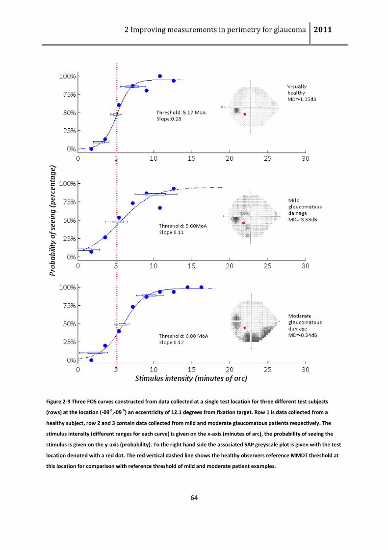
2 Improving measurements in perimetry for glaucoma 2011
64
Figure 2-9 Three FOS curves constructed from data collected at a single test location for three different test subjects
(rows) at the location (-09 o
,-09 o
) an eccentricity of 12.1 degrees from fixation target. Row 1 is data collected from a
healthy subject, row 2 and 3 contain data collected from mild and moderate glaucomatous patients respectively. The
stimulus intensity (different ranges for each curve) is given on the x-axis (minutes of arc), the probability of seeing the
stimulus is given on the y-axis (probability). To the right hand side the associated SAP greyscale plot is given with the test
location denoted with a red dot. The red vertical dashed line shows the healthy observers reference MMDT threshold at
this location for comparison with reference threshold of mild and moderate patient examples.
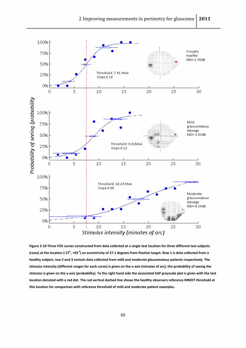
2 Improving measurements in perimetry for glaucoma 2011
65
Figure 2-10 Three FOS curves constructed from data collected at a single test location for three different test subjects
(rows) at the location (-27o, +03
o) an eccentricity of 27.1 degrees from fixation target. Row 1 is data collected from a
healthy subject, row 2 and 3 contain data collected from mild and moderate glaucomatous patients respectively. The
stimulus intensity (different ranges for each curve) is given on the x-axis (minutes of arc), the probability of seeing the
stimulus is given on the y-axis (probability). To the right hand side the associated SAP greyscale plot is given with the test
location denoted with a red dot. The red vertical dashed line shows the healthy observers reference MMDT threshold at
this location for comparison with reference threshold of mild and moderate patient examples.
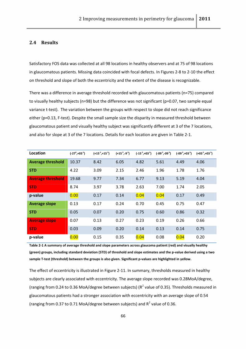
2 Improving measurements in perimetry for glaucoma 2011
66
2.4 Results
Satisfactory FOS data was collected at all 98 locations in healthy observers and at 75 of 98 locations
in glaucomatous patients. Missing data coincided with focal defects. In Figures 2-8 to 2-10 the effect
on threshold and slope of both the eccentricity and the extent of the disease is recognizable.
There was a difference in average threshold recorded with glaucomatous patients (n=75) compared
to visually healthy subjects (n=98) but the difference was not significant (p=0.07, two sample equal
variance t-test). The variation between the groups with respect to slope did not reach significance
either (p=0.13, F-test). Despite the small sample size the disparity in measured threshold between
glaucomatous patient and visually healthy subject was significantly different at 3 of the 7 locations,
and also for slope at 3 of the 7 locations. Details for each location are given in Table 2-1.
Location (-27o,+03 o) (+15 o,+15 o) (+15 o,-9 o) (-15 o,+03 o) (-09 o,-09 o) (-09 o,+03 o) (+03 o,+03 o)
Average threshold 10.37 8.42 6.05 4.82 5.61 4.49 4.06
STD 4.22 3.09 2.15 2.46 1.96 1.78 1.76
Average threshold 19.68 9.77 7.34 6.77 9.13 5.19 4.04
STD 8.74 3.97 3.78 2.63 7.00 1.74 2.05
p-value 0.00 0.17 0.14 0.04 0.04 0.17 0.49
Average slope 0.13 0.17 0.24 0.70 0.45 0.75 0.47
STD 0.05 0.07 0.20 0.75 0.60 0.86 0.32
Average slope 0.07 0.13 0.27 0.23 0.19 0.26 0.66
STD 0.03 0.09 0.20 0.14 0.13 0.14 0.75
p-value 0.00 0.15 0.35 0.04 0.08 0.04 0.20
Table 2-1 A summary of average threshold and slope parameters across glaucoma patient (red) and visually healthy
(green) groups, including standard deviation (STD) of threshold and slope estimates and the p-value derived using a two
sample T-test (threshold) between the groups is also given. Significant p-values are highlighted in yellow.
The effect of eccentricity is illustrated in Figure 2-11. In summary, thresholds measured in healthy
subjects are clearly associated with eccentricity. The average slope recorded was 0.28MoA/degree,
(ranging from 0.24 to 0.36 MoA/degree between subjects) (R2 value of 0.35). Thresholds measured in
glaucomatous patients had a stronger association with eccentricity with an average slope of 0.54
(ranging from 0.37 to 0.71 MoA/degree between subjects) and R2 value of 0.36.
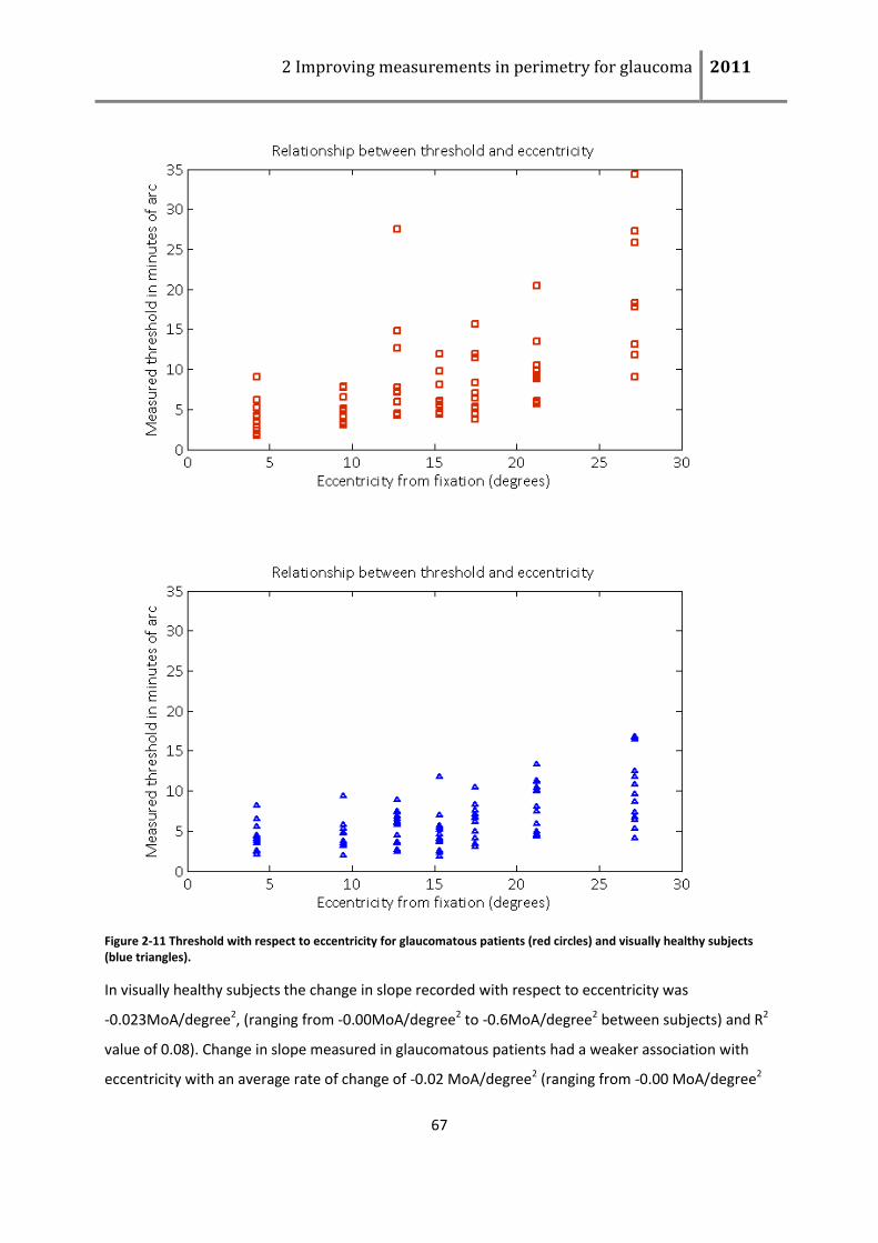
2 Improving measurements in perimetry for glaucoma 2011
67
Figure 2-11 Threshold with respect to eccentricity for glaucomatous patients (red circles) and visually healthy subjects (blue triangles).
In visually healthy subjects the change in slope recorded with respect to eccentricity was
-0.023MoA/degree2, (ranging from -0.00MoA/degree2 to -0.6MoA/degree2 between subjects) and R2
value of 0.08). Change in slope measured in glaucomatous patients had a weaker association with
eccentricity with an average rate of change of -0.02 MoA/degree2 (ranging from -0.00 MoA/degree2
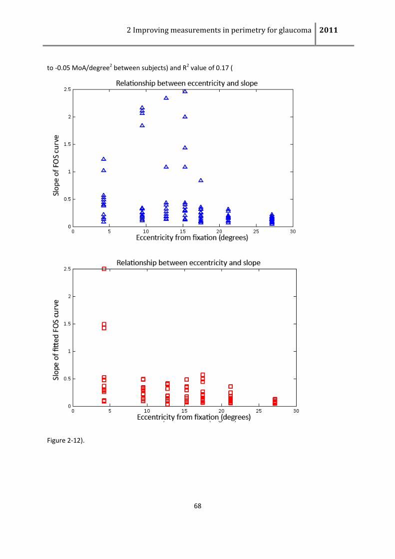
2 Improving measurements in perimetry for glaucoma 2011
68
to -0.05 MoA/degree2 between subjects) and R2 value of 0.17 (
Figure 2-12).
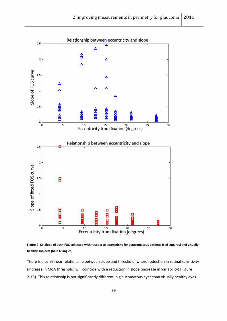
2 Improving measurements in perimetry for glaucoma 2011
69
Figure 2-12 Slope of each FOS collected with respect to eccentricity for glaucomatous patients (red squares) and visually
healthy subjects (blue triangles).
There is a curvilinear relationship between slope and threshold, where reduction in retinal sensitivity
(increase in MoA threshold) will coincide with a reduction in slope (increase in variability) (Figure
2-13). This relationship is not significantly different in glaucomatous eyes than visually healthy eyes.
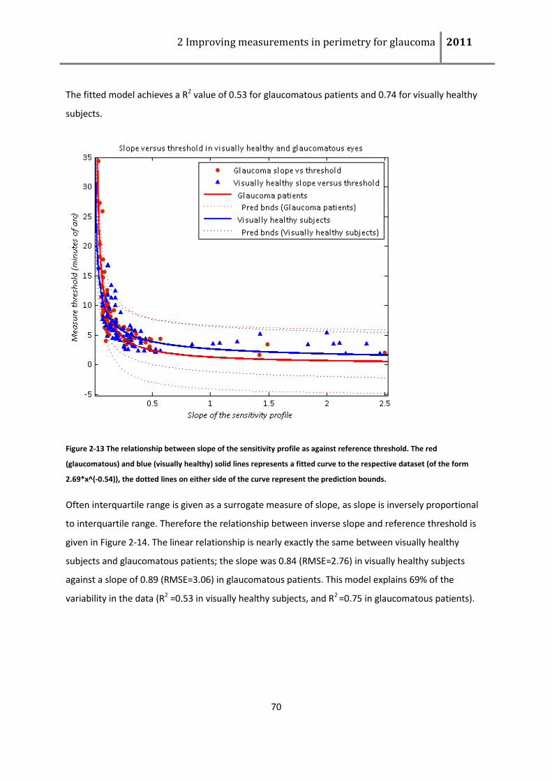
2 Improving measurements in perimetry for glaucoma 2011
70
The fitted model achieves a R2 value of 0.53 for glaucomatous patients and 0.74 for visually healthy
subjects.
Figure 2-13 The relationship between slope of the sensitivity profile as against reference threshold. The red
(glaucomatous) and blue (visually healthy) solid lines represents a fitted curve to the respective dataset (of the form
2.69*x^(-0.54)), the dotted lines on either side of the curve represent the prediction bounds.
Often interquartile range is given as a surrogate measure of slope, as slope is inversely proportional
to interquartile range. Therefore the relationship between inverse slope and reference threshold is
given in Figure 2-14. The linear relationship is nearly exactly the same between visually healthy
subjects and glaucomatous patients; the slope was 0.84 (RMSE=2.76) in visually healthy subjects
against a slope of 0.89 (RMSE=3.06) in glaucomatous patients. This model explains 69% of the
variability in the data (R2 =0.53 in visually healthy subjects, and R2 =0.75 in glaucomatous patients).
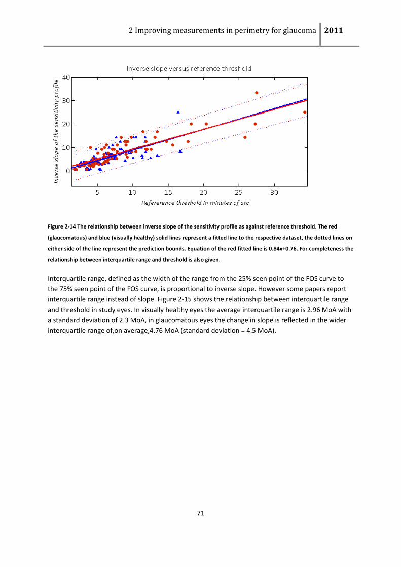
2 Improving measurements in perimetry for glaucoma 2011
71
Figure 2-14 The relationship between inverse slope of the sensitivity profile as against reference threshold. The red
(glaucomatous) and blue (visually healthy) solid lines represent a fitted line to the respective dataset, the dotted lines on
either side of the line represent the prediction bounds. Equation of the red fitted line is 0.84x+0.76. For completeness the
relationship between interquartile range and threshold is also given.
Interquartile range, defined as the width of the range from the 25% seen point of the FOS curve to
the 75% seen point of the FOS curve, is proportional to inverse slope. However some papers report
interquartile range instead of slope. Figure 2-15 shows the relationship between interquartile range
and threshold in study eyes. In visually healthy eyes the average interquartile range is 2.96 MoA with
a standard deviation of 2.3 MoA, in glaucomatous eyes the change in slope is reflected in the wider
interquartile range of,on average,4.76 MoA (standard deviation = 4.5 MoA).
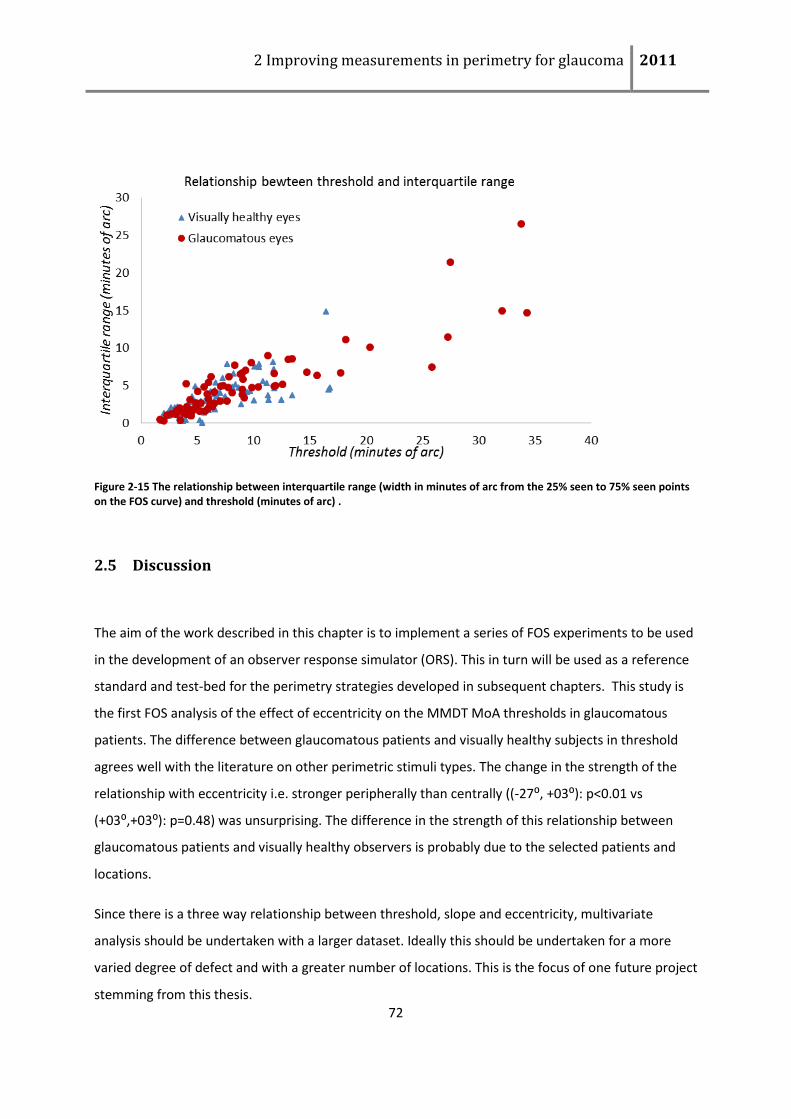
2 Improving measurements in perimetry for glaucoma 2011
72
Figure 2-15 The relationship between interquartile range (width in minutes of arc from the 25% seen to 75% seen points on the FOS curve) and threshold (minutes of arc) .
2.5 Discussion
The aim of the work described in this chapter is to implement a series of FOS experiments to be used
in the development of an observer response simulator (ORS). This in turn will be used as a reference
standard and test-bed for the perimetry strategies developed in subsequent chapters. This study is
the first FOS analysis of the effect of eccentricity on the MMDT MoA thresholds in glaucomatous
patients. The difference between glaucomatous patients and visually healthy subjects in threshold
agrees well with the literature on other perimetric stimuli types. The change in the strength of the
relationship with eccentricity i.e. stronger peripherally than centrally ((-27⁰, +03⁰): p<0.01 vs
(+03⁰,+03⁰): p=0.48) was unsurprising. The difference in the strength of this relationship between
glaucomatous patients and visually healthy observers is probably due to the selected patients and
locations.
Since there is a three way relationship between threshold, slope and eccentricity, multivariate
analysis should be undertaken with a larger dataset. Ideally this should be undertaken for a more
varied degree of defect and with a greater number of locations. This is the focus of one future project
stemming from this thesis.
2 Improving measurements in perimetry for glaucoma 2011
73
Despite the sizeable differences between the setup used by Westcott and colleagues (1998) and
those implemented in this study, the results of this experiment agree well with those reported
previously. Examining the location at 15 degrees eccentricity within this experiment with those
collected previously (albeit in a different quadrant but with the same eccentricity), we find good
agreement between the average thresholds (visually healthy subjects 4.8±2.5MoA vs. 5.9±1.7MoA
glaucomatous patients 6.8 ± 2.6MoA vs. 8.7 ± 3.4MoA). Slopes are not reported by Westcott and
colleagues but rather the inter-quartile ranges (3.39 ± 1.4 in visually healthy subjects vs. 5.39 ±2.3 in
glaucomatous patients), again showing good agreement with the current study.
The difference in slope between the patients and visually healthy subjects is not surprising and
reflects conclusions from several studies that previously described the reduction in slope with
decreased retinal sensitivity in DLS (Henson et al., 2000, Chauhan et al., 1993). The high correlation
between slope and threshold shown here suggests that this is true also with the MMDT stimulus
type.
The thresholds and slopes vary considerably between subjects which is representative of the true
population. Since the ORS will estimate for each subject (set of FOS curves) independently and since
ideally we want to examine a wide range of subjects, this was not perceived as a disadvantage. It was
concluded that FOS curves constructed would serve as an adequate estimate of observer responses
and would provide reasonable estimates of true threshold for simulation work as described by others
(Turpin et al., 2003).
Using the Psignifit module provides an independent methodology for eliminating the underlying
models which are less suitable for fitting the collected data. For example, the Gaussian was less
suitable than the Weibull. Furthermore Psignifit offers more reliable information on width of the
confidence intervals around threshold with the addition of the ‘worst’ CI based on sensitivity analysis
(Wichmann and Hill, 2001b). Finally Psignifit offers estimates on how well the turning points of the
FOS curve were assessed. There are more conventional methods of fitting the psychometric function.
One of these, Probit analysis, relies on an underlying Gaussian distribution in the model for the FOS
curve. However the estimate of error (the standard deviation) is calculated directly from empirical
data, which again would be fine if the data sets were large (and sampling scheme was correct). In
most psychophysical settings this is not the case, and substantial errors have been reported in Probit
estimates of variability (Foster & Bischof, 1987, 1991; McKee, Klein, & Teller, 1985).
2 Improving measurements in perimetry for glaucoma 2011
74
Adaptive frequency of seeing data collection methodologies may have significant advantages to the
standard MOCS approach, manifesting mostly in the reduction in required number of presentations
and subsequent reduction in test duration. The adaptive probit estimation (APE) approach as
described by Watt and Andrews (Watt and Andrews, 1981) or the Bayesian adaptive procedure of
Kontsevich and Tyler (Kontsevich and Tyler 1999) ,for example, outlines two such methods. In each
an adaptive approach to the choice of stimulus intensity presented is used, where presentations are
focused at the level of threshold. Intermediate assessment of threshold and slope is derived during
data acquisition and when variability falls within an acceptable level then testing is terminated.
However, with the adaptive probit approach it has been shown that there is associated bias and the
Probit fit used to calculate the variability may not be the correct model. Kaernbach and colleagues
also suggested an adaptive approach which focused presentations on the turning points of the
curves achieving quicker more reliable estimates than that of the APE methodology (Kaernbach,
2001). A more recent study by Turpin et al. (Turpin, McKendrick, 2010) has examined the Bayesian
approach to FOS data collection but further examination of bias is required. The study described in
this chapter did not aim to look at a ‘quick’ FOS method, but this is the subject of future work. But a
comparison with such a method against sampling using MOCS would be useful, because there is no
doubt that the latter is onerous even for people who are relatively experienced in psychophysics. The
main objective of this study was to gather FOS responses on the multi-locational MMDT to ‘fuel’ the
ORS, which in turn was used to develop the test strategies at the centre of this thesis. The idea was
to follow that approach used by others to test performance of test strategies notably Turpin (Turpin
et al., 2003) and accordingly to use this information on performance to iteratively test and improve
new test strategies. There are limitations to every ORS even when based on FOS data. Some of the
perceived limitations of the ORS originate from the assumption that the FOS curves do not change
with fatigue and learning effects are negligible. In addition, the FOS data was collected at only seven
locations and thus is not ideal for generation of a full field patient simulator. Still, the data gathered
here is useful since it provides, at least, a direct method of isolating the threshold algorithm most
likely to have highest efficiency for testing.
3 Developing and evaluating clinically useful threshold search
methods
The work described in this chapter, outlines the performance of clinical threshold search method
which was implemented on the MMDT. The results here have been presented in part as a poster
presentation at the Association for Research in Vision and Ophthalmology Meeting, Fort Lauderdale,
Florida, USA in May 2008 and, again in part, as a read paper at the 18th International Symposium of
the Imaging and Perimetry Society Meeting in Nara, Japan in May 2008 (See ‘List of supporting
publications’).
Using real patients to examine testing strategies is time consuming and difficult. Moreover, it is
impossible to know the true threshold because it is ever changing with respect to attention
(Carrasco, 2006), alertness (Henson and Emuh, 2010), eye movement and other factors. Testing real
observers and patients will be the ultimate aim of a clinical threshold search but should be reserved
for final stage assessment. A good method to objectively examine the accuracy and bias of any
threshold search method is with computer simulation. The sole limitation of this methodology is
accepted (Treutwein, 1995), namely: Does the chosen observer model represent real observers
behaviour? The previous chapter described how data was carefully collected to build an ORS used in
some of the studies described in the following chapters.
By using FOS curves derived in chapter 2 it is possible to measure error of clinical threshold search
methods in two ways. One approach allows FOS curves to provide a “reference threshold” in a cohort
of subjects, this reference standard can then be compared to threshold estimates yielded using
clinical search methods collected directly from the same cohort. This will be referred to as the
patient data approach. Alternatively the ORS approach utilises simulated observer responses directly
from the underlying probability function of the respective FOS curve. The latter can be used to
generate a series of patient trials with each clinical search method, returning a distribution of
possible threshold values. Estimates of error and efficiency can be derived from this data.
The methods and formulae used to calculate error and efficiency are provided below. Next, an
overview of the possible testing strategies and details of the necessary adaptations to the MMDT are
given. In the second half of this chapter reports the results of both methods, firstly the patient data
approach followed by the ORS approach.
3 Improving measurements in perimetry for glaucoma 2011
76
3.1 Estimating measurement error and efficiency
To detect differences in the performance between clinical test methods and threshold search
methods in particular, certain summary measures are helpful. In this chapter the reference threshold
was derived from the constructed FOS curves outlined in chapter 2. Bias is the average difference
between measured threshold and reference threshold. Equation 3-1 was used to calculate bias,
denoted B. The total number of trials with one variant of a clinical search method completed
(reaching termination) with ORS is denoted by n (in the patient data approach n is equal to 1).
denotes reference threshold as estimated from the constructed FOS curve at location i. is the
threshold as estimated from a clinical threshold search method.
Equation 3-1 Bias at one location
∑
Precision is a summary measure of the amount of variance in the estimate of threshold which is
unaffected by bias, denoted by P in Equation 3-2. For example if a method returns an estimate of
threshold which is consistently within a small range of values, this will have high precision even if
these values are not close to reference threshold.
Equation 3-2 Precision at one location
√
∑ ̅
Accuracy is the average variance between estimated threshold and reference threshold. This
combines bias and precision.
Equation 3-3 Accuracy
√
∑ ( )
Test duration can be measured in two ways the test duration in seconds or the number of
presentations required. In this chapter, in the patient data approach, average time per location as
3 Improving measurements in perimetry for glaucoma 2011
77
recorded within the software, for the ORS approach the number of presentations will be used, in the
latter case it is denoted TD and di denotes the total number of presentations during the ith simulated
threshold search.
Equation 3-4 Test Duration
∑
Efficiency is a parameter which combines time and accuracy, and in short summaries the
performance. Time and accuracy are weighted differently according to the requirements of the test;
there is debate on ideal efficiency, however in this case the simplest option was chosen.
Equation 3-5 Efficiency
3.2 Review of established threshold search methods
Method of constant stimuli (MOCS) can be thought of as a reference technique to obtain sensitivity
data (Fechner, 1860). It is reliable, providing data for threshold estimation; however for frequent use
it is impractical due to the long test duration.
The method of limits (Fechner, 1860) uses an up-down method to reach threshold estimation. In
predefined sized steps, the intensity is increased/decreased from one end of the range to the other
and then reversed and decreased/increased back through the range of intensities.
All threshold search methods including those employed in clinical use are really variants of these
basic approaches. Three questions determine the signatory attributes of a threshold search method:
what intensity level to set the next presentation; when to finish testing; and how to estimate
threshold from the collected data. Threshold search methods work under the assumption that the
underlying psychometric function is monotonic and continuous. Threshold, slope, FP and FN are
allowed to vary independently within predefined limits e.g. FP + FN < 1.
3 Improving measurements in perimetry for glaucoma 2011
78
3.2.1 Non parametric methods
A modification of the method of limits is the truncated method of limits, sometimes referred to as an
up-down staircase. Here step direction is altered with a change in response (direction - when steps
from incremented to decrementing or vice versa, this is known as a reversal). Therefore the
presentations are centred about threshold. This method for threshold search (without the estimation
of slope), had significant time saving properties over the MOCS or method of limits, by reducing the
number of necessary presentations by 30-40% (Dixon and Mood, 1948).
Staircases, truncated staircases, transformed up-down methods (Levitt, 1971), non-parametric up-
down (Derman, 1957), weighted up-down (Kaernbach, 1991), MOBS (Tyrrell and Owens, 1988),
stochastic approximation (Robbins and Monro, 1951) and PEST (Taylor and Creelman, 1967) (PEST
uses heuristic rules) are all variants of the methods of limits. In each, the number of reversals, step
size and/or how the threshold is estimated from the collected data varies. Every psychometric
threshold search method was developed to answer a particular need in psychometric testing;
Treutwein offers an elegant overview of each (Treutwein, 1995).
The advantages of non-parametric threshold search methods are numerous: they are, by design,
unbiased by priors, can be designed to terminate quicker for patients than parametric threshold
search methods. The disadvantages being that if they have been designed to terminate quicker for
patients, then visually healthy subjects will sometimes take longer to test, due to the proportion of
presentations directed toward the abnormal end of the scale. They are reportedly less precise in
threshold estimation throughout the whole range in comparison to parametric methods.
Staircases have formed the backbone of clinical threshold search methods since the 1970’s (Heijl,
1977, Heijl and Drance, 1980, Heijl, 1985a). For example, Full Threshold (FT) on the HFA is a
truncated staircase of the 4-2 variety (Heijl et al., 1987). In this case, the first presentation will occur
on, or near to the average value from normative data (or estimate from seed locations). Then, the
search method will take a step (ascending or descending; based on the response given) of four
decibels (dB), steps of size four dB will continue until the reversal occurs. On reversal, step size
changes and drops to two dB, on the next reversal the threshold search terminates.
3 Improving measurements in perimetry for glaucoma 2011
79
3.2.2 Parametric threshold search methods
In SAP, the underlying psychometric function is monotonically decreasing and continuous (in the case
of the MMDT it is monotonically increasing), in parametric methods some prior knowledge of the
general form of the psychometric function is required. This means that some template such as a
cumulative Gaussian, is assumed to fit the data, then one or two variables forming this model are
allowed to vary and are estimated from the collected data. Parametric methods were developed to
help circumvent heuristic rules used to set intermediate intensity levels. Theoretically the dynamic
terminating criteria based on “goodness of fit” allowed with parametric methods (rather than
presentation number or number of reversals) should isolate those cases where further data
collection would be beneficial (Treutwein, 1997).
These methods use a range of templates, or mathematical functions, to set a general form of the
psychometric function (e.g. Gaussian, Beta, Gamma, logistic or more typically Weibull). Data is
collected to inform the best guess estimate of the prior. Parametric methods are of two main types:
maximum likelihood (Pentland, 1980, Lieberman and Pentland, 1982) or Bayesian methods (Watson
and Pelli, 1979, Watson and Pelli, 1983, King-Smith et al., 1994). In maximum likelihood threshold
search methods, the search begins with the first presentation (start point) at the best estimate of
threshold (e.g. population based mean). An estimate of the likelihood of data collected in a given trial
belonging to a set of population values is maintained. For example, given the set of possible
threshold values, the likelihood of each threshold is calculated and the most plausible threshold is
selected. In Bayesian methodology the best guess estimate takes the form of a prior distribution
rather than estimate for the start point. Bayesian methods advance by multiplying the prior by the
likelihood function resulting in the updated likelihood function. Based on the prior selected, and
responses recorded, the step size/stimulus intensities will vary with both methodologies. The
terminating criteria can be based on number of reversals but can be based on goodness of fit
(Treutwein, 1997).
Parametric methods have recently been accepted as alternative quicker clinical threshold search
methods compared to the standard staircases. For example, the so called zippy estimation with
3 Improving measurements in perimetry for glaucoma 2011
80
sequential testing (ZEST) on the FDT Matrix is a Bayesian method (Anderson et al., 2005). The prior
was uniform and thus could not affect the threshold measure. The procedure was terminated after
four presentations as there was no perceived gain in precision (Anderson, 2003b).
3.2.3 Including spatial information in clinical threshold search methods
The visual field does not consist of a discrete number of locations, but rather of a vast number of
possible test locations with relationship between test locations defined by the underlying physiology
of the retinal nerve fibre layer. For example, to extrapolate the sensitivity at locations between test
locations, an interpolation of sensitivity estimates is performed after the test terminates to form the
familiar greyscale plot. The loss of retinal ganglion cells in glaucoma and associated sensitivity loss is
observed to follow the nerve fibre pattern (Hubel and Wiesel, 1960, Caprioli and Miller, 1989,
Morgan et al., 1998, Weber and Ulrich, 1990). There have been several studies examining the
structure function relationship in glaucomatous patients (Hood et al., 2007, Garway-Heath et al.,
2002, Harwerth et al., 2004). Whilst the relationship is not as strong as historically expected
(probably due to measurement noise and poor understanding of the measures as outlined in section
1.4.3), there is a significant association (Bowd et al., 2006). Therefore, if a low sensitivity is recorded
at a given location, Tp, it follows that in those locations shown to be associated with Tp, there is an
increased likelihood these locations will have reduced sensitivity (Heijl et al., 1989, Heijl and Asman,
1989, Crabb et al., 1997, Gardiner et al., 2004, Spry et al., 2002, Crabb et al., 1995, Chauhan et al.,
1989).
Sensibly, some clinical threshold search methods have been designed to use this ‘spatial’ information
to help improve performance. To achieve this, response information from surrounding locations is
allowed to influence intermediate threshold estimates of Tp. A seed location, for example, as
implemented in the full threshold methodology of the HFA, is one such example. In this scenario
there are four seed locations placed at (±09⁰, ±09⁰) and the test procedure begins with examination
of them. When threshold estimates of these locations are reached, the general height of the HoV is
set. Depending on whether this estimate is an under or over estimate of the height of HoV, every
location will require more presentations to cross the point of subjective equivalence, which due to
the probabilistic nature of the test it is less likely to achieve. Therefore, the bias introduced by the
3 Improving measurements in perimetry for glaucoma 2011
81
seed locations will remain in the estimate of every threshold. Considering a patient with high central
sensitivity and low peripheral sensitivity the increased variability introduced becomes apparent.
Tendency oriented perimetry (TOP), as implemented in the Octopus perimeter, presents a stimulus
at each location once, but threshold estimation is adjusted at each location four times. Estimates of
threshold are updated continuously, using linear interpolation of the neighbours tested, the test
advances by using a bracketing approach. In this case the bias is clearly apparent as the defects
recorded have been reported to be shallower, have softer edges and are smaller (Morales et al.,
2000). Another study indicated that the defect may be weighted out completely (Anderson, 2003a).
SITA offers an attractive alternative to FT. The reduction in test duration is derived from the partial
Bayesian approach taken, requiring fewer presentations overall, but also significantly from the
absence of catch trials. Again in SITA the seed locations set the general height of the HoV. An
empirical Bayesian approach is implemented at each test location. At each location two parameters
are maintained, threshold estimate and classification (‘defective’ or ‘non-defective’). The eight
closest neighbours contribute to the classification, while only the four closest neighbours contribute
to the estimate of threshold. Neighbours were derived from a “non-homogenous directional
dependence” between locations from an unpublished map developed by Airaksinen and colleagues
(Department of Ophthalmology, University of Oulu, Finland). The technique is underpinned by a
spatial model used in imaging reconstruction. Detail of the SITA algorithm has been published
(Olsson and Rootzén, 1994) but exact reproduction of the SITA method has not been achieved as
some of the necessary detail is unclear or missing. However, it is recognised that a Bayesian
approach is used and that the priors implemented do have a significant influence over threshold
estimate, in some cases the observer responses have less influence than prior used (Rootzén and
Olsson, 2006). Turpin and colleagues have investigated their SITA-like threshold extensively and have
shown that the bias introduced is equivalent (or less) than that in a full threshold methodology
(Turpin et al., 2003).
3.2.4 Efficiency in clinical threshold search methods
To have an efficient threshold search method the slope of the underlying sensitivity profile should be
fixed and the search for the position of threshold should be the only unknown. In this case the
3 Improving measurements in perimetry for glaucoma 2011
82
experimenter supplies not only the template of the psychometric function (general form) but also
the slope and the other parameters (FN, FP). In this case the possible psychometric functions are
single parameter translations of one another. However, it is clear that this is not true of the MMDT
stimulus type and measurement scale, as shown in chapter 2, nor is it true with DLS (Wall et al.,
1996). To achieve this in practice the x-axis (stimulus intensity) would have to be scaled
appropriately; as subjects at either end of the scale of sensitivity should then require the same
number of presentations to go from seen to unseen. In this case, the number of presentations would
be reduced for glaucomatous patients and the relative difference between intensities would be
closer to being standardised. Since there are less presentations and migration from seen to unseen is
quicker, the overall test time should be shorter, response confidence should be elevated and
together these should reduce the lapse and guess rates. The Dynamic strategy of the Octopus
perimeter attempts this type of strategy and reports similar results to the FT method with shorter
test duration (Weber, 1995). However it is not possible to implement this type of strategy correctly
without extensive FOS data collection in a large cohort of visually healthy subjects and glaucomatous
patients. It is also likely that there would be variation of the shape of the psychometric function
between disease types.
As mentioned, each threshold search method will be affected by prior information used. In some
cases population based priors can improve efficiency. Seed locations introduce bias, but spatial
information can improve performance, if applied correctly (Turpin et al., 2003). Ultimately spatial
information and priors should influence the starting point but should not influence the final estimate
of threshold. However, each method will be affected to varying degrees by these parameters
depending on how far the chosen initiation point of the search is from true threshold. Terminating
criteria will also affect performance, and as such will be different for each different search method.
Typical terminating criteria include the number of presentations (Anderson et al., 2005), the number
of reversals (Harvey, 1997) or difference between the prior and posterior mean/mode (Treutwein,
1997). The terminating criteria will largely decide the amount of data collected at a given test
location. The more data collected at a given location, the more accurate the estimate of threshold.
Estimates of threshold can be derived from collected data in several ways, however recording the of
the average of stimulus intensity at the last two reversal points is commonly used. The mean/median
of the posterior function is an option with parametric threshold search methods. Considering that
each perimetric stimulus type has a differently shaped FOS curve which will change with eccentricity
and glaucomatous damage, it is reasonable to assume that search methods which perform well with
3 Improving measurements in perimetry for glaucoma 2011
83
one stimulus type may not perform well with another. By adjusting the step size, start point,
terminating criterion and process of estimating threshold, the final estimate of threshold will be
significantly affected. Physical restrictions of the hardware will often influence these parameters (e.g.
step size or start point) and the measurement scales will differ significantly between stimuli types.
Therefore, in terms of threshold search strategies, one size does not fit all.
3.3 Threshold testing for the MMDT
As outlined in chapter 2, the MMDT is a perimetry test, restricted by the pixel pitch of the monitor.
The size of the pixel pitch determines the number of the possible steps that cover the test range.
Furthermore while pixel pitch is uniform across the screen, the angle subtended is not. Any selected
test strategy would have to hold this as a consideration. Simple staircases, like 2-1 (step size halved
on first reversal e.g. 2dB initial step size with 1dB step size on reversal) and 1-1 (same step size
before and after reversals) were selected as possibilities and these were the original methods used
with the MMDT (Verdon-Roe, 2006). Strategies like ASA, PEST, MOBS and several other variations
can also be eliminated because of their demands to half the step size on reversal.
The aim of the work described in this chapter is to examine the performance of three possible clinical
search strategies for the MMDT. The strategies investigated included a 1-1 staircase and a 2-1
staircase which are the current test strategies on the MDT against a new strategy WEBS, details of
which are described below.
3.3.1 Weight based search (WEBS)
WEBS utilises some of the properties of modified binary search (MOBS)) (Tyrrell and Owens, 1988).
With MOBS, threshold is filtered using a progressive bisection of the intensity range according to
responses given. For example, with a negative response the lower half the range is selected, the mid-
point of this range is chosen as the next stimulus presentation intensity etc. The ordered list of
presentation intensities displayed describes the search path. With the WEBS strategy, threshold is
filtered similarly; however the partitions are not uniform across the range, in this case divisions are
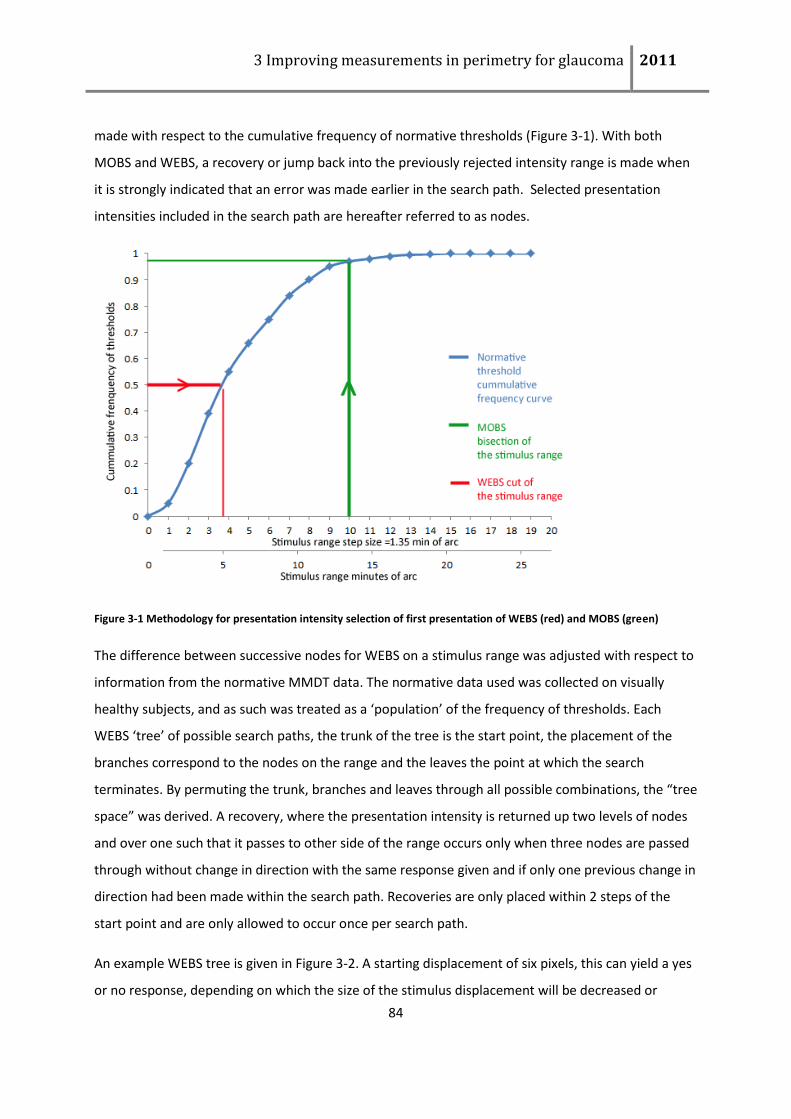
3 Improving measurements in perimetry for glaucoma 2011
84
made with respect to the cumulative frequency of normative thresholds (Figure 3-1). With both
MOBS and WEBS, a recovery or jump back into the previously rejected intensity range is made when
it is strongly indicated that an error was made earlier in the search path. Selected presentation
intensities included in the search path are hereafter referred to as nodes.
Figure 3-1 Methodology for presentation intensity selection of first presentation of WEBS (red) and MOBS (green)
The difference between successive nodes for WEBS on a stimulus range was adjusted with respect to
information from the normative MMDT data. The normative data used was collected on visually
healthy subjects, and as such was treated as a ‘population’ of the frequency of thresholds. Each
WEBS ‘tree’ of possible search paths, the trunk of the tree is the start point, the placement of the
branches correspond to the nodes on the range and the leaves the point at which the search
terminates. By permuting the trunk, branches and leaves through all possible combinations, the “tree
space” was derived. A recovery, where the presentation intensity is returned up two levels of nodes
and over one such that it passes to other side of the range occurs only when three nodes are passed
through without change in direction with the same response given and if only one previous change in
direction had been made within the search path. Recoveries are only placed within 2 steps of the
start point and are only allowed to occur once per search path.
An example WEBS tree is given in Figure 3-2. A starting displacement of six pixels, this can yield a yes
or no response, depending on which the size of the stimulus displacement will be decreased or
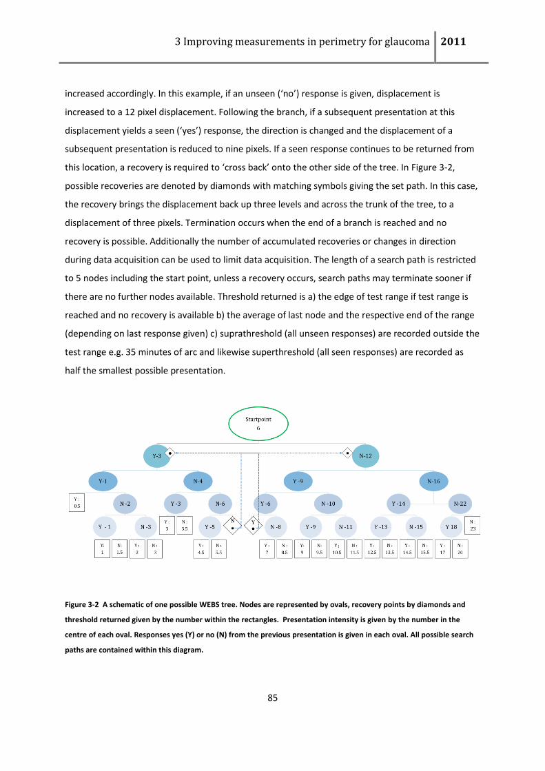
3 Improving measurements in perimetry for glaucoma 2011
85
increased accordingly. In this example, if an unseen (‘no’) response is given, displacement is
increased to a 12 pixel displacement. Following the branch, if a subsequent presentation at this
displacement yields a seen (‘yes’) response, the direction is changed and the displacement of a
subsequent presentation is reduced to nine pixels. If a seen response continues to be returned from
this location, a recovery is required to ‘cross back’ onto the other side of the tree. In Figure 3-2,
possible recoveries are denoted by diamonds with matching symbols giving the set path. In this case,
the recovery brings the displacement back up three levels and across the trunk of the tree, to a
displacement of three pixels. Termination occurs when the end of a branch is reached and no
recovery is possible. Additionally the number of accumulated recoveries or changes in direction
during data acquisition can be used to limit data acquisition. The length of a search path is restricted
to 5 nodes including the start point, unless a recovery occurs, search paths may terminate sooner if
there are no further nodes available. Threshold returned is a) the edge of test range if test range is
reached and no recovery is available b) the average of last node and the respective end of the range
(depending on last response given) c) suprathreshold (all unseen responses) are recorded outside the
test range e.g. 35 minutes of arc and likewise superthreshold (all seen responses) are recorded as
half the smallest possible presentation.
Figure 3-2 A schematic of one possible WEBS tree. Nodes are represented by ovals, recovery points by diamonds and
threshold returned given by the number within the rectangles. Presentation intensity is given by the number in the
centre of each oval. Responses yes (Y) or no (N) from the previous presentation is given in each oval. All possible search
paths are contained within this diagram.
3 Improving measurements in perimetry for glaucoma 2011
86
The shape of the tree determines the possible routes to termination. The product of number of
presentations to reach termination with the underlying probably density function of normative data
is averaged (over all simulations) to derive an efficiency coefficient. A comparison of these efficiency
coefficients for all possible trees is used to optimise the layout of the branches of the tree. This
provides a systematic a method to select strategy which will produce the most likely outcomes in the
shortest amount of time (quick for visually healthy subjects). Subsequently the normative data
distribution was adjusted to include a proportion of glaucomatous eyes to ensure that unseen
locations would terminate quickly and this optimisation process was repeated.
The restrictions that will affect the possible shapes (possible positions of the nodes) of the trees are
different step sizes (screen resolution), start point (corresponding to a set point on the normative
range e.g. 90% limit of normality), termination criteria and types of recoveries allowed. With the ORS
approach it is possible investigate the tree space that comprises a set number of increments of each
of these restrictions and the effect they have on the strategy. In the simulations reported here the
90% limit of normality was selected as the choice of start point; terminating criteria was as described
above; step sizes varied from 0.5 minutes of arc up to 2.5minutes of arc. These limits were selected
to correspond to current screen resolutions, e.g. a step size of 0.5 minutes of arc, corresponds to
screen resolution that is greater than is currently available (pixel pitch of 0.05mm, at location -
27⁰,+03⁰ at a test distance of 30cm). On the other end of this range a step size of 2.5 minutes of arc
this would correspond to a typical screen with pixel pitch of 0.22mm (corresponds approximately to a
15.4” laptop screen with SXGA display).
3.4 Testing the strategies: Patient data approach
Participants in the study detailed in Chapter 2 underwent additional testing on a different date but
within three months of the FOS data collection. This cohort of subjects consisted of 14 visually
healthy and 14 glaucomatous patients whom were invited to return for a study examining the
performance of threshold algorithms. The age range of the patients was 36 to 79 years with an
average age of 65 years. Average MD was -3.82dB [range -8.24dB to 0.57dB]. The age range of the
healthy observers was 37 to 79 years with an average age of 65 years. Average MD for the visually
healthy observers was -0.36dB [range -1.82dB to 1.39dB]. Inclusion and exclusion criteria for the
*
Y T=1
3 Improving measurements in perimetry for glaucoma 2011
87
healthy observers and the glaucomatous patients recruited for this study were as described in
section 2.3.1. The study was approved by Moorfields ethics committee and conformed to the
Declaration of Helsinki with all participants giving their informed written consent.
Each subject undertook one examination with each of the following test strategies, in a randomised
test order. The first trial algorithm was a 1-1 staircase with second reversal triggering termination,
threshold returned was the average of the last two reversal points. The second trial algorithm was
the 2-1 staircase with second reversal triggering termination, threshold returned was the average of
the last two reversal points. The third method was WEBS as outlined above in section 3.3.
The reference threshold at seven locations (namely (-27⁰,+03⁰), (-15⁰,+03⁰), (-9⁰,+03⁰), (+03⁰,+03⁰),
(-09⁰,-09⁰), (+09⁰, -15⁰), (+15⁰,+15⁰)) calculated from the FOS data collection from 98/98 locations in
healthy subjects and 75/98 in glaucomatous patients (the reduced number of locations with FOS data
in glaucomatous patients is due to a test location coinciding with a focal defect). Bias, precision, and
test duration were calculated for the four different strategies tested in the study outlined above in
section 3.1.
3.4.1 Results
The summary measures of bias and precision are shown for three clinical threshold search methods
in visually healthy subjects in Figure 3-2. Precision varies between strategies, the 1-1 staircase was
significantly more precise than 2-1 or WEBS (p<0.01; Krusal-Wallis test), and 2-1 was significantly
more precise than WEBS (p=0.05; Krusal-Wallis test). There is a relationship between increase in
reference threshold and an underestimation of threshold to varying degrees with all strategies,
however WEBS was least affected.
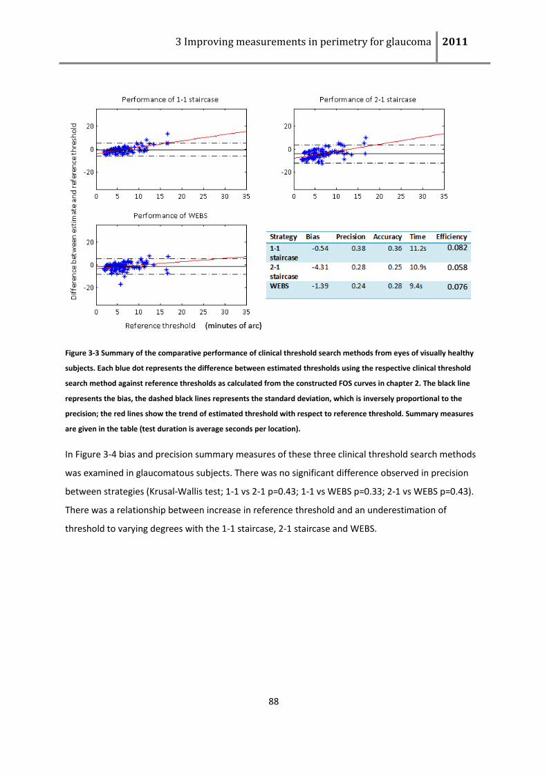
3 Improving measurements in perimetry for glaucoma 2011
88
Figure 3-3 Summary of the comparative performance of clinical threshold search methods from eyes of visually healthy
subjects. Each blue dot represents the difference between estimated thresholds using the respective clinical threshold
search method against reference thresholds as calculated from the constructed FOS curves in chapter 2. The black line
represents the bias, the dashed black lines represents the standard deviation, which is inversely proportional to the
precision; the red lines show the trend of estimated threshold with respect to reference threshold. Summary measures
are given in the table (test duration is average seconds per location).
In Figure 3-4 bias and precision summary measures of these three clinical threshold search methods
was examined in glaucomatous subjects. There was no significant difference observed in precision
between strategies (Krusal-Wallis test; 1-1 vs 2-1 p=0.43; 1-1 vs WEBS p=0.33; 2-1 vs WEBS p=0.43).
There was a relationship between increase in reference threshold and an underestimation of
threshold to varying degrees with the 1-1 staircase, 2-1 staircase and WEBS.
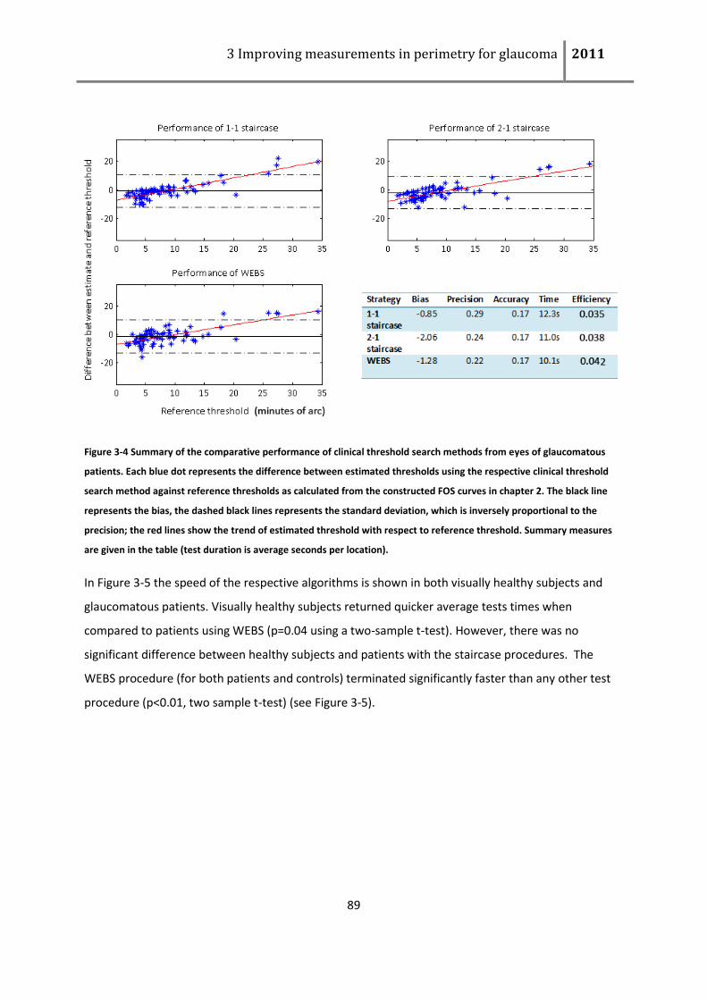
3 Improving measurements in perimetry for glaucoma 2011
89
Figure 3-4 Summary of the comparative performance of clinical threshold search methods from eyes of glaucomatous
patients. Each blue dot represents the difference between estimated thresholds using the respective clinical threshold
search method against reference thresholds as calculated from the constructed FOS curves in chapter 2. The black line
represents the bias, the dashed black lines represents the standard deviation, which is inversely proportional to the
precision; the red lines show the trend of estimated threshold with respect to reference threshold. Summary measures
are given in the table (test duration is average seconds per location).
In Figure 3-5 the speed of the respective algorithms is shown in both visually healthy subjects and
glaucomatous patients. Visually healthy subjects returned quicker average tests times when
compared to patients using WEBS (p=0.04 using a two-sample t-test). However, there was no
significant difference between healthy subjects and patients with the staircase procedures. The
WEBS procedure (for both patients and controls) terminated significantly faster than any other test
procedure (p<0.01, two sample t-test) (see Figure 3-5).
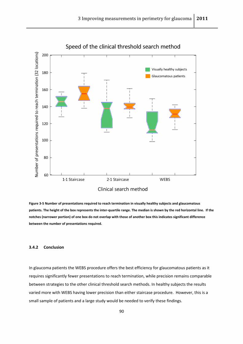
3 Improving measurements in perimetry for glaucoma 2011
90
Figure 3-5 Number of presentations required to reach termination in visually healthy subjects and glaucomatous
patients. The height of the box represents the inter-quartile range. The median is shown by the red horizontal line. If the
notches (narrower portion) of one box do not overlap with those of another box this indicates significant difference
between the number of presentations required.
3.4.2 Conclusion
In glaucoma patients the WEBS procedure offers the best efficiency for glaucomatous patients as it
requires significantly fewer presentations to reach termination, while precision remains comparable
between strategies to the other clinical threshold search methods. In healthy subjects the results
varied more with WEBS having lower precision than either staircase procedure. However, this is a
small sample of patients and a large study would be needed to verify these findings.
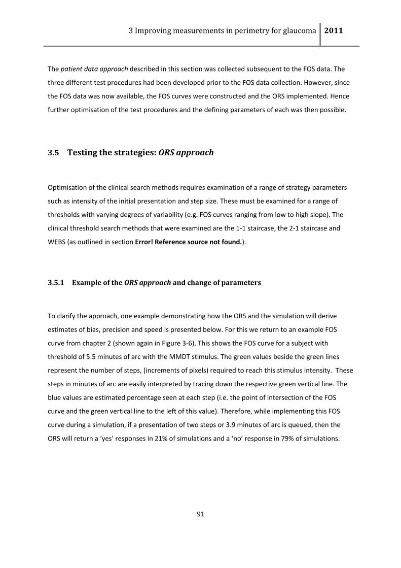
3 Improving measurements in perimetry for glaucoma 2011
91
The patient data approach described in this section was collected subsequent to the FOS data. The
three different test procedures had been developed prior to the FOS data collection. However, since
the FOS data was now available, the FOS curves were constructed and the ORS implemented. Hence
further optimisation of the test procedures and the defining parameters of each was then possible.
3.5 Testing the strategies: ORS approach
Optimisation of the clinical search methods requires examination of a range of strategy parameters
such as intensity of the initial presentation and step size. These must be examined for a range of
thresholds with varying degrees of variability (e.g. FOS curves ranging from low to high slope). The
clinical threshold search methods that were examined are the 1-1 staircase, the 2-1 staircase and
WEBS (as outlined in section Error! Reference source not found.).
3.5.1 Example of the ORS approach and change of parameters
To clarify the approach, one example demonstrating how the ORS and the simulation will derive
estimates of bias, precision and speed is presented below. For this we return to an example FOS
curve from chapter 2 (shown again in Figure 3-6). This shows the FOS curve for a subject with
threshold of 5.5 minutes of arc with the MMDT stimulus. The green values beside the green lines
represent the number of steps, (increments of pixels) required to reach this stimulus intensity. These
steps in minutes of arc are easily interpreted by tracing down the respective green vertical line. The
blue values are estimated percentage seen at each step (i.e. the point of intersection of the FOS
curve and the green vertical line to the left of this value). Therefore, while implementing this FOS
curve during a simulation, if a presentation of two steps or 3.9 minutes of arc is queued, then the
ORS will return a ‘yes’ responses in 21% of simulations and a ‘no’ response in 79% of simulations.
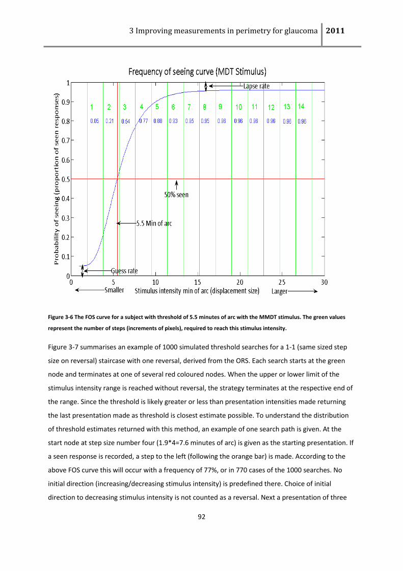
3 Improving measurements in perimetry for glaucoma 2011
92
Figure 3-6 The FOS curve for a subject with threshold of 5.5 minutes of arc with the MMDT stimulus. The green values
represent the number of steps (increments of pixels), required to reach this stimulus intensity.
Figure 3-7 summarises an example of 1000 simulated threshold searches for a 1-1 (same sized step
size on reversal) staircase with one reversal, derived from the ORS. Each search starts at the green
node and terminates at one of several red coloured nodes. When the upper or lower limit of the
stimulus intensity range is reached without reversal, the strategy terminates at the respective end of
the range. Since the threshold is likely greater or less than presentation intensities made returning
the last presentation made as threshold is closest estimate possible. To understand the distribution
of threshold estimates returned with this method, an example of one search path is given. At the
start node at step size number four (1.9*4=7.6 minutes of arc) is given as the starting presentation. If
a seen response is recorded, a step to the left (following the orange bar) is made. According to the
above FOS curve this will occur with a frequency of 77%, or in 770 cases of the 1000 searches. No
initial direction (increasing/decreasing stimulus intensity) is predefined there. Choice of initial
direction to decreasing stimulus intensity is not counted as a reversal. Next a presentation of three
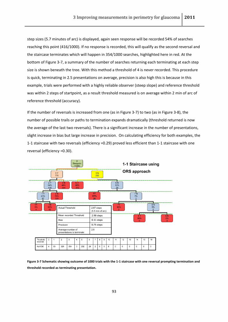
3 Improving measurements in perimetry for glaucoma 2011
93
step sizes (5.7 minutes of arc) is displayed, again seen response will be recorded 54% of searches
reaching this point (416/1000). If no response is recorded, this will qualify as the second reversal and
the staircase terminates which will happen in 354/1000 searches, highlighted here in red. At the
bottom of Figure 3-7, a summary of the number of searches returning each terminating at each step
size is shown beneath the tree. With this method a threshold of 4 is never recorded. This procedure
is quick, terminating in 2.5 presentations on average, precision is also high this is because in this
example, trials were performed with a highly reliable observer (steep slope) and reference threshold
was within 2 steps of startpoint, as a result threshold measured is on average within 2 min of arc of
reference threshold (accuracy).
If the number of reversals is increased from one (as in Figure 3-7) to two (as in Figure 3-8), the
number of possible trails or paths to termination expands dramatically (threshold returned is now
the average of the last two reversals). There is a significant increase in the number of presentations,
slight increase in bias but large increase in precision. On calculating efficiency for both examples, the
1-1 staircase with two reversals (efficiency =0.29) proved less efficient than 1-1 staircase with one
reversal (efficiency =0.30).
Figure 3-7 Schematic showing outcome of 1000 trials with the 1-1 staircase with one reversal prompting termination and
threshold recorded as terminating presentation.
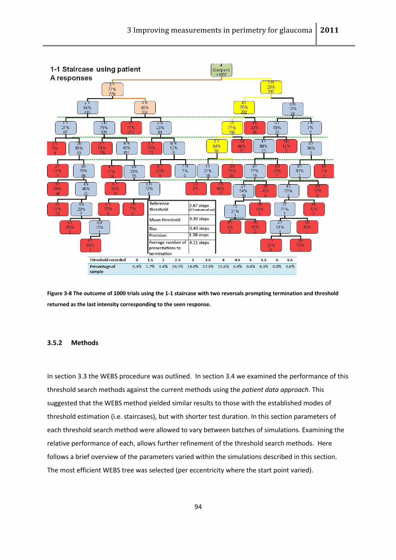
3 Improving measurements in perimetry for glaucoma 2011
94
Figure 3-8 The outcome of 1000 trials using the 1-1 staircase with two reversals prompting termination and threshold
returned as the last intensity corresponding to the seen response.
3.5.2 Methods
In section 3.3 the WEBS procedure was outlined. In section 3.4 we examined the performance of this
threshold search methods against the current methods using the patient data approach. This
suggested that the WEBS method yielded similar results to those with the established modes of
threshold estimation (i.e. staircases), but with shorter test duration. In this section parameters of
each threshold search method were allowed to vary between batches of simulations. Examining the
relative performance of each, allows further refinement of the threshold search methods. Here
follows a brief overview of the parameters varied within the simulations described in this section.
The most efficient WEBS tree was selected (per eccentricity where the start point varied).
3 Improving measurements in perimetry for glaucoma 2011
95
The Start point was set at the 90% limit of normality according to the normative database for the
MDT, the relative effect of start point on each threshold algorithm in terms of bias, precision and test
duration was examined.
The Step size which is the minimum possible displacement (in the conventional perimetry this would
equate to the minimum increment in contrast e.g. in the HFA II it is 2dB) was set to 5 step sizes to
examine the effect of step size on each threshold algorithm in terms of bias and precision namely:
0.5 minutes of arc; 1 minute of arc; 1.5minutes of arc; 2 minutes of arc and 2.5 minutes of arc. Step
size is of particular importance to the MMDT as it is determined absolutely by the pixel pitch of the
monitor.
The terminating criteria, staircases employed the number of reversals as the only terminating
criteria (two reversals was selected as three was too long to be comparable to WEBS). A WEBS
search path terminated if there were no further nodes available between end of the range and the
previous node or alternatively if the search path exceeded four nodes.
The method used to record threshold, here for staircases strategies the average of the last two
reversal points or in cases where one end of the range was reached the last seen/unseen
presentation was returned as threshold. For WEBS: threshold returned is a) the edge of test range if
test range is reached and no recovery is available b) the average of last node and the respective
(depending on last response given) end of the range. For all strategies the supra-threshold outcomes
(all unseen responses) are recorded outside the test range e.g. 35 minutes of arc and likewise super-
threshold outcomes (all seen responses) are recorded as half the smallest possible presentation.
For each FOS curve 1,000 simulations of each combination were performed. Summary measures of
bias, precision, accuracy, test duration and efficiency were calculated using the formulae outlined in
section 3.1. For example in Figure 3-9 the box and whisker plot of the outcomes of 1,000 simulations
for each of the three strategies for one FOS curve are shown. Bias summarises the distance from
estimated threshold to reference threshold. Accuracy is a summary measure of the spread of the
box and whiskers.
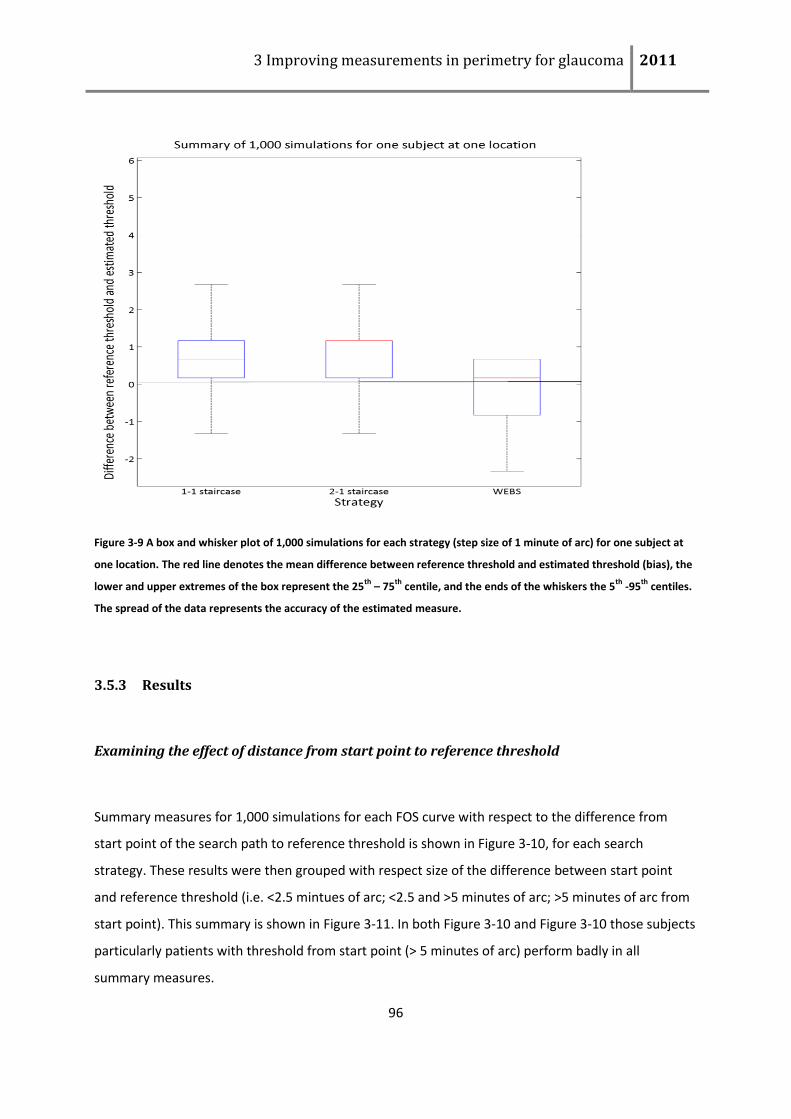
3 Improving measurements in perimetry for glaucoma 2011
96
Figure 3-9 A box and whisker plot of 1,000 simulations for each strategy (step size of 1 minute of arc) for one subject at
one location. The red line denotes the mean difference between reference threshold and estimated threshold (bias), the
lower and upper extremes of the box represent the 25th
– 75th
centile, and the ends of the whiskers the 5th
-95th
centiles.
The spread of the data represents the accuracy of the estimated measure.
3.5.3 Results
Examining the effect of distance from start point to reference threshold
Summary measures for 1,000 simulations for each FOS curve with respect to the difference from
start point of the search path to reference threshold is shown in Figure 3-10, for each search
strategy. These results were then grouped with respect size of the difference between start point
and reference threshold (i.e. <2.5 mintues of arc; <2.5 and >5 minutes of arc; >5 minutes of arc from
start point). This summary is shown in Figure 3-11. In both Figure 3-10 and Figure 3-10 those subjects
particularly patients with threshold from start point (> 5 minutes of arc) perform badly in all
summary measures.
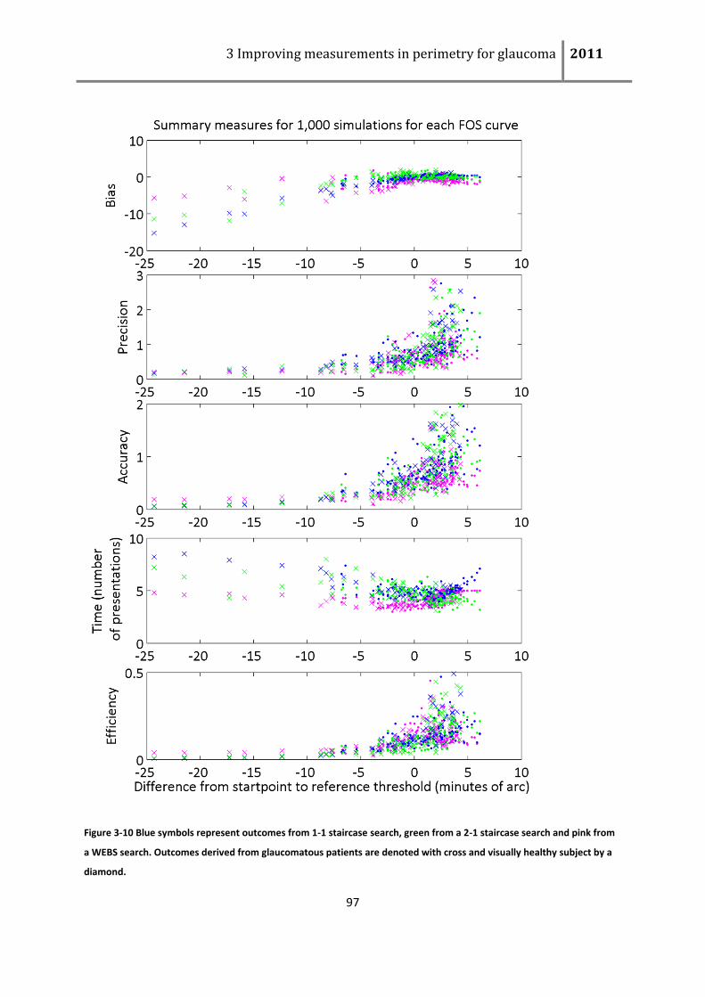
3 Improving measurements in perimetry for glaucoma 2011
97
Figure 3-10 Blue symbols represent outcomes from 1-1 staircase search, green from a 2-1 staircase search and pink from
a WEBS search. Outcomes derived from glaucomatous patients are denoted with cross and visually healthy subject by a
diamond.
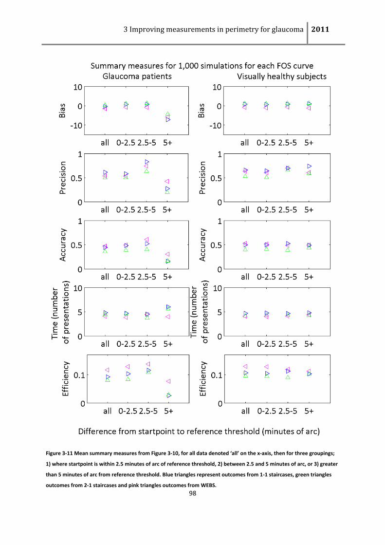
3 Improving measurements in perimetry for glaucoma 2011
98
Figure 3-11 Mean summary measures from Figure 3-10, for all data denoted ‘all’ on the x-axis, then for three groupings;
1) where startpoint is within 2.5 minutes of arc of reference threshold, 2) between 2.5 and 5 minutes of arc, or 3) greater
than 5 minutes of arc from reference threshold. Blue triangles represent outcomes from 1-1 staircases, green triangles
outcomes from 2-1 staircases and pink triangles outcomes from WEBS.
3 Improving measurements in perimetry for glaucoma 2011
99
In Figure 3-10 and Figure 3-11, it is apparent that WEBS is consistently faster than either staircase.
Bias is also much reduced with WEBS versus either staircase and in particularly for those FOS curves
where reference threshold is far from start point. Precision appears to be similar between the
groups, accuracy is low over all. There is a marked difference in accuracy between those with start
point greater than 5 minutes of arc above threshold and the other groups.
Examining the effect of Step size
In Figure 3-12, the effect of step size on efficiency each of the threshold strategies is examined. The
mean of all data irrespective of reference threshold is reported under grouping labelled ‘all’. Those
FOS curves with start point within 2.5 minutes of arc of reference threshold are reported under the
group labelled ‘0-2.5’. Those FOS curves with start point greater than 2.5 minutes of arc but less than
5 minutes of arc from reference threshold are reported under the group labelled ‘2.5-5’. Lastly those
FOS curves with start point greater than 5 minutes of arc from reference threshold are reported
under the group labelled ‘5+’. With FOS curves yielded from glaucoma patients, these groups
contained 41, 23 and 11 datasets respectively, and for FOS curves yielded from visually healthy
subjects, these groups contained 51, 38 and 8 datasets respectively. In most cases WEBS yields
higher efficiency especially for glaucomatous patients with start point far from reference threshold.
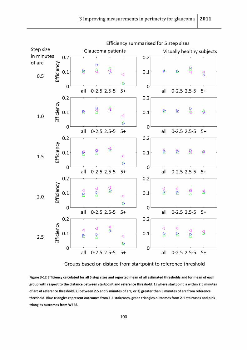
3 Improving measurements in perimetry for glaucoma 2011
100
Figure 3-12 Efficiency calculated for all 5 step sizes and reported mean of all estimated thresholds and for mean of each
group with respect to the distance between startpoint and reference threshold. 1) where startpoint is within 2.5 minutes
of arc of reference threshold, 2) between 2.5 and 5 minutes of arc, or 3) greater than 5 minutes of arc from reference
threshold. Blue triangles represent outcomes from 1-1 staircases, green triangles outcomes from 2-1 staircases and pink
triangles outcomes from WEBS.
3 Improving measurements in perimetry for glaucoma 2011
101
3.5.4 Conclusion
Distance from start point to reference threshold and step size impact the performance of clinical
threshold search methods. In the experiment described above, which was designed to meet the
needs of the MMDT, WEBS has greater test efficiency than either staircase procedure. Where start
point is far from reference threshold, there is increased bias and reduced precision, both of which
negatively impact accuracy, which in turn affect efficiency. With increased step size efficiency is
lowered for staircases but increased for WEBS. However, with patients with elevated threshold (start
point far from reference threshold) WEBS always had higher efficiency than staircases, this has
important implications for clinic based testing.
3.6 Discussion
The results agree well between the patient data approach and ORS approach in both cases the WEBS
had greater efficiency than either staircase strategy for glaucomatous eyes.
Each threshold estimation regardless on the distance from start point is important, ideally uniform
accuracy should be obtained at each possible threshold value. However, with a start point far below
threshold, particularly with staircases, the demand of a large number of responses to reach the point
of subjective equivalence introduces bias. For 2-1 staircase with start point set close to the mean of
the normative data will have much wider confidence intervals than a 1-1 staircase (with the same
start point )at the normal end of the scale and the converse is true when the start point is far from
threshold. In terms of perimetry the 4-2 staircase used in full threshold search method in the HVFA
would have much wider confidence limits in comparison to a 2-2 staircase at the ‘normal’ end of the
measurement scale, but the 2-2 would have greater bias at the abnormal end of the scale. This is
reduced with the use of prior information, in the example shown in Figure 3-10 and Figure 3-11, the
WEBS procedures were less affected by start point in terms of bias. This is of considerable
importance when assessing threshold in eyes with pathology, since they are likely to have threshold
values far from the start point set. This, at least in part, explains the large repeatability issues at the
lower end of the scale with the HFVA and the full threshold algorithm (Henson et al., 2000).
3 Improving measurements in perimetry for glaucoma 2011
102
While step size is a restriction of all perimetric instruments, step size has a large effect on
performance of threshold search methods and it has been somewhat overlooked in the published
literature. The work presented in this chapter may prompt FOS study to address this question in DLS
standard automated perimetry.
Most published simulation work uses FOS curves with estimates of threshold and slope derived
variability limits (Henson et al., 2000, Turpin and McKendrick, 2003, Turpin et al., 2002a, Turpin et al.,
2002b, Turpin et al., 2003, McKendrick and Turpin, 2005a). Since the data reported by Henson and
colleagues (2000) is derived with a threshold search method (full threshold) this will confound the
simulation work by introducing variability which originates from the threshold search method rather
than the patient. The FOS curves used in this work were carefully derived from visually healthy
subjects and glaucomatous patients at a large number of locations. It rendered the responses
generated by the ORS to be potentially more representative of real patient responses.
Additional factors influencing patient data approach, like fatigue and learning effect have not been
incorporated in the simulations reported in this chapter. These would be useful to implement, but
implement would be very difficult to assess properly.
Highly variable subjects (those with shallow FOS curves) produced low accuracy perimetric exams
outcomes. This will produce a large degree of noise in the measures confounds detection of
progression. In these cases regardless of the test strategy used this low signal to noise ratio likely will
persist and the overall test accuracy will remain low. Identifying these subjects at baseline and
eliminating them from threshold examination or adapting the test to a suprathreshold test in
locations of damage may prove a more efficient approach to data collection.
4 Developing and evaluating a case-finding perimetry algorithm
The full-threshold (FT) testing strategy used in automated perimetry has been a standard
measurement for mapping the extent and depth of visual field defects, especially in a hospital or
secondary/tertiary care setting. However, the patient examination time for this clinical test is long
and measurements yielded are still often unacceptably variable. Over the years attempts have been
made to develop faster and more efficient test strategies as discussed in chapter three (Turpin and
McKendrick, 2003, McKendrick and Turpin, 2005b, Turpin et al., 2007, Anderson and Johnson, 2006,
Morales et al., 2000, Weber and Klimaschka, 1995). There is a need to have a quick visual field test
while maintaining acceptable specificity and sensitivity, especially for glaucoma detection in primary
care, screening programmes and large epidemiological studies (Vitale et al., 2000, Quigley, 1998,
Henson and Artes, 2002, Henson et al., 1998, Quigley et al., 2007). In these settings, perimeters
employing suprathreshold (ST) testing strategies are typically used. Suprathreshold measurements
are simple: stimuli are presented to the subject, one at a time, typically at a level above the
estimated detection threshold of a normal visual field location. Normally, if a presentation at any
location is recorded as unseen, then later in the test another presentation (trial) is made at that same
location. If both presentations at a given location are unseen, then that point is classified as a defect.
ST offers simple pass/fail results to the clinician. Furthermore stimulus presentations are displayed at
the upper levels of the normal response (bright) and are displayed less frequently at each location:
for the test subject naïve to perimetry this improves test acceptability and eases understanding
(Gardiner et al., 2008, Artes et al., 2002a).
Not all ST testing strategies are limited to two trials and it would seem sensible, especially when the
aim is to minimise false positive diagnosis of a defective location, to have more trials per location
(multisampling). Artes and colleagues (Artes et al., 2003, Artes et al., 2002a) examined this idea
rigorously, concluding that measured VF defect area was less variable and exhibited lower systematic
error when using multisampling suprathreshold paradigms (3 or even 5 trials at each point). The
method has been implemented in Henson Pro perimeter (Sheen Instruments, Surrey, UK). Still, the
benefit of increased sampling at all test points does come at the cost of increased test time
compared to conventional ST.
This chapter describes the design of novel method of suprathreshold testing (Enhanced
Suprathreshold Testing Algorithm (ESTA)), which was developed with the aim of maintaining short
test duration, without negatively affecting diagnostic precision. This aim was pursued by exploiting
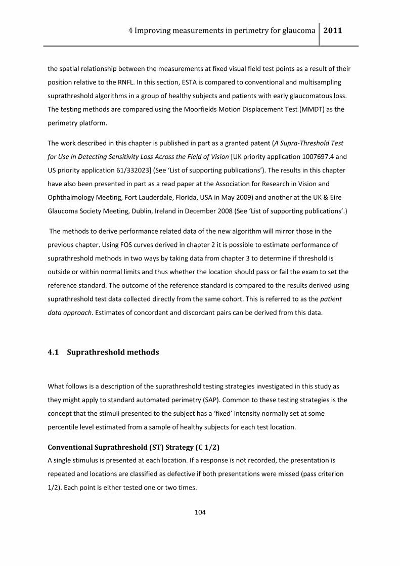
4 Improving measurements in perimetry for glaucoma 2011
104
the spatial relationship between the measurements at fixed visual field test points as a result of their
position relative to the RNFL. In this section, ESTA is compared to conventional and multisampling
suprathreshold algorithms in a group of healthy subjects and patients with early glaucomatous loss.
The testing methods are compared using the Moorfields Motion Displacement Test (MMDT) as the
perimetry platform.
The work described in this chapter is published in part as a granted patent (A Supra-Threshold Test
for Use in Detecting Sensitivity Loss Across the Field of Vision [UK priority application 1007697.4 and
US priority application 61/332023] (See ‘List of supporting publications’). The results in this chapter
have also been presented in part as a read paper at the Association for Research in Vision and
Ophthalmology Meeting, Fort Lauderdale, Florida, USA in May 2009) and another at the UK & Eire
Glaucoma Society Meeting, Dublin, Ireland in December 2008 (See ‘List of supporting publications’.)
The methods to derive performance related data of the new algorithm will mirror those in the
previous chapter. Using FOS curves derived in chapter 2 it is possible to estimate performance of
suprathreshold methods in two ways by taking data from chapter 3 to determine if threshold is
outside or within normal limits and thus whether the location should pass or fail the exam to set the
reference standard. The outcome of the reference standard is compared to the results derived using
suprathreshold test data collected directly from the same cohort. This is referred to as the patient
data approach. Estimates of concordant and discordant pairs can be derived from this data.
4.1 Suprathreshold methods
What follows is a description of the suprathreshold testing strategies investigated in this study as
they might apply to standard automated perimetry (SAP). Common to these testing strategies is the
concept that the stimuli presented to the subject has a ‘fixed’ intensity normally set at some
percentile level estimated from a sample of healthy subjects for each test location.
Conventional Suprathreshold (ST) Strategy (C 1/2)
A single stimulus is presented at each location. If a response is not recorded, the presentation is
repeated and locations are classified as defective if both presentations were missed (pass criterion
1/2). Each point is either tested one or two times.
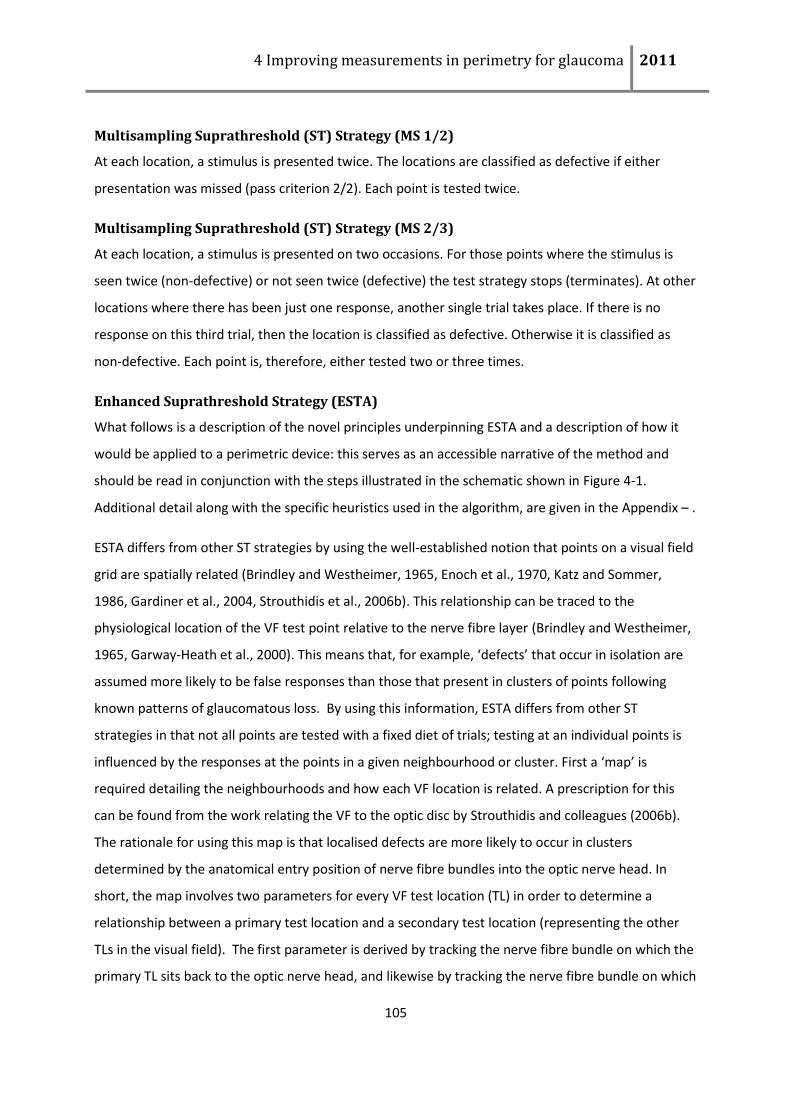
4 Improving measurements in perimetry for glaucoma 2011
105
Multisampling Suprathreshold (ST) Strategy (MS 1/2)
At each location, a stimulus is presented twice. The locations are classified as defective if either
presentation was missed (pass criterion 2/2). Each point is tested twice.
Multisampling Suprathreshold (ST) Strategy (MS 2/3)
At each location, a stimulus is presented on two occasions. For those points where the stimulus is
seen twice (non-defective) or not seen twice (defective) the test strategy stops (terminates). At other
locations where there has been just one response, another single trial takes place. If there is no
response on this third trial, then the location is classified as defective. Otherwise it is classified as
non-defective. Each point is, therefore, either tested two or three times.
Enhanced Suprathreshold Strategy (ESTA)
What follows is a description of the novel principles underpinning ESTA and a description of how it
would be applied to a perimetric device: this serves as an accessible narrative of the method and
should be read in conjunction with the steps illustrated in the schematic shown in Figure 4-1.
Additional detail along with the specific heuristics used in the algorithm, are given in the Appendix – .
ESTA differs from other ST strategies by using the well-established notion that points on a visual field
grid are spatially related (Brindley and Westheimer, 1965, Enoch et al., 1970, Katz and Sommer,
1986, Gardiner et al., 2004, Strouthidis et al., 2006b). This relationship can be traced to the
physiological location of the VF test point relative to the nerve fibre layer (Brindley and Westheimer,
1965, Garway-Heath et al., 2000). This means that, for example, ‘defects’ that occur in isolation are
assumed more likely to be false responses than those that present in clusters of points following
known patterns of glaucomatous loss. By using this information, ESTA differs from other ST
strategies in that not all points are tested with a fixed diet of trials; testing at an individual points is
influenced by the responses at the points in a given neighbourhood or cluster. First a ‘map’ is
required detailing the neighbourhoods and how each VF location is related. A prescription for this
can be found from the work relating the VF to the optic disc by Strouthidis and colleagues (2006b).
The rationale for using this map is that localised defects are more likely to occur in clusters
determined by the anatomical entry position of nerve fibre bundles into the optic nerve head. In
short, the map involves two parameters for every VF test location (TL) in order to determine a
relationship between a primary test location and a secondary test location (representing the other
TLs in the visual field). The first parameter is derived by tracking the nerve fibre bundle on which the
primary TL sits back to the optic nerve head, and likewise by tracking the nerve fibre bundle on which
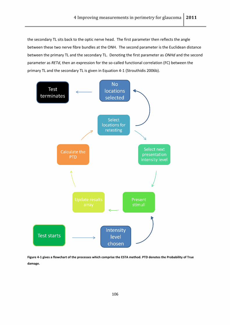
4 Improving measurements in perimetry for glaucoma 2011
106
the secondary TL sits back to the optic nerve head. The first parameter then reflects the angle
between these two nerve fibre bundles at the ONH. The second parameter is the Euclidean distance
between the primary TL and the secondary TL. Denoting the first parameter as ONHd and the second
parameter as RETd, then an expression for the so-called functional correlation (FC) between the
primary TL and the secondary TL is given in Equation 4-1 (Strouthidis 2006b).
Figure 4-1 gives a flowchart of the processes which comprise the ESTA method. PTD denotes the Probability of True
damage.
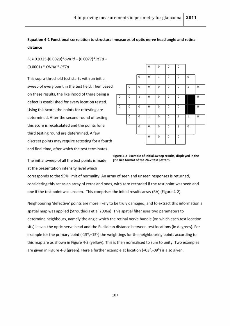
4 Improving measurements in perimetry for glaucoma 2011
107
Equation 4-1 Functional correlation to structural measures of optic nerve head angle and retinal
distance
FC= 0.9325-(0.0029)*ONHd – (0.0077)*RETd +
(0.0001) * ONHd * RETd
This supra-threshold test starts with an initial
sweep of every point in the test field. Then based
on these results, the likelihood of there being a
defect is established for every location tested.
Using this score, the points for retesting are
determined. After the second round of testing
this score is recalculated and the points for a
third testing round are determined. A few
discreet points may require retesting for a fourth
and final time, after which the test terminates.
The initial sweep of all the test points is made
at the presentation intensity level which
corresponds to the 95% limit of normality. An array of seen and unseen responses is returned,
considering this set as an array of zeros and ones, with zero recorded if the test point was seen and
one if the test point was unseen. This comprises the initial results array (RA) (Figure 4-2).
Neighbouring ‘defective’ points are more likely to be truly damaged, and to extract this information a
spatial map was applied (Strouthidis et al 2006a). This spatial filter uses two parameters to
determine neighbours, namely the angle which the retinal nerve bundle (on which each test location
sits) leaves the optic nerve head and the Euclidean distance between test locations (in degrees). For
example for the primary point (-15⁰,+15⁰) the weightings for the neighbouring points according to
this map are as shown in Figure 4-3 (yellow). This is then normalised to sum to unity. Two examples
are given in Figure 4-3 (green). Here a further example at location (+03⁰,-09⁰) is also given.
0 0 0 0
0 0 1 0 0 0
0 0 0 0 0 0 1 0
0 0 1 0 0 0 0 0
0 0 0 0 0 0 0 0
0 0 1 0 0 1 1 0
0 0 0 0 1 0
0 0 0 0
Figure 4-2 Example of initial sweep results, displayed in the grid like format of the 24-2 test pattern.
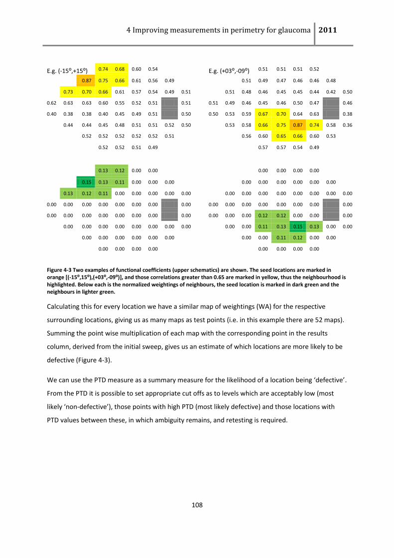
4 Improving measurements in perimetry for glaucoma 2011
108
E.g. (-15⁰,+15⁰) 0.74 0.68 0.60 0.54 E.g. (+03⁰,-09⁰) 0.51 0.51 0.51 0.52
0.87 0.75 0.66 0.61 0.56 0.49 0.51 0.49 0.47 0.46 0.46 0.48
0.73 0.70 0.66 0.61 0.57 0.54 0.49 0.51 0.51 0.48 0.46 0.45 0.45 0.44 0.42 0.50
0.62 0.63 0.63 0.60 0.55 0.52 0.51 0.51 0.51 0.49 0.46 0.45 0.46 0.50 0.47 0.46
0.40 0.38 0.38 0.40 0.45 0.49 0.51 0.50 0.50 0.53 0.59 0.67 0.70 0.64 0.63 0.38
0.44 0.44 0.45 0.48 0.51 0.51 0.52 0.50 0.53 0.58 0.66 0.75 0.87 0.74 0.58 0.36
0.52 0.52 0.52 0.52 0.52 0.51 0.56 0.60 0.65 0.66 0.60 0.53
0.52 0.52 0.51 0.49 0.57 0.57 0.54 0.49
0.13 0.12 0.00 0.00 0.00 0.00 0.00 0.00
0.15 0.13 0.11 0.00 0.00 0.00 0.00 0.00 0.00 0.00 0.00 0.00
0.13 0.12 0.11 0.00 0.00 0.00 0.00 0.00 0.00 0.00 0.00 0.00 0.00 0.00 0.00 0.00
0.00 0.00 0.00 0.00 0.00 0.00 0.00 0.00 0.00 0.00 0.00 0.00 0.00 0.00 0.00 0.00
0.00 0.00 0.00 0.00 0.00 0.00 0.00 0.00 0.00 0.00 0.00 0.12 0.12 0.00 0.00 0.00
0.00 0.00 0.00 0.00 0.00 0.00 0.00 0.00 0.00 0.00 0.11 0.13 0.15 0.13 0.00 0.00
0.00 0.00 0.00 0.00 0.00 0.00 0.00 0.00 0.11 0.12 0.00 0.00
0.00 0.00 0.00 0.00 0.00 0.00 0.00 0.00
Figure 4-3 Two examples of functional coefficients (upper schematics) are shown. The seed locations are marked in orange [(-15⁰,15⁰),(+03⁰,-09⁰)], and those correlations greater than 0.65 are marked in yellow, thus the neighbourhood is highlighted. Below each is the normalized weightings of neighbours, the seed location is marked in dark green and the neighbours in lighter green.
Calculating this for every location we have a similar map of weightings (WA) for the respective
surrounding locations, giving us as many maps as test points (i.e. in this example there are 52 maps).
Summing the point wise multiplication of each map with the corresponding point in the results
column, derived from the initial sweep, gives us an estimate of which locations are more likely to be
defective (Figure 4-3).
We can use the PTD measure as a summary measure for the likelihood of a location being ‘defective’.
From the PTD it is possible to set appropriate cut offs as to levels which are acceptably low (most
likely ‘non-defective’), those points with high PTD (most likely defective) and those locations with
PTD values between these, in which ambiguity remains, and retesting is required.
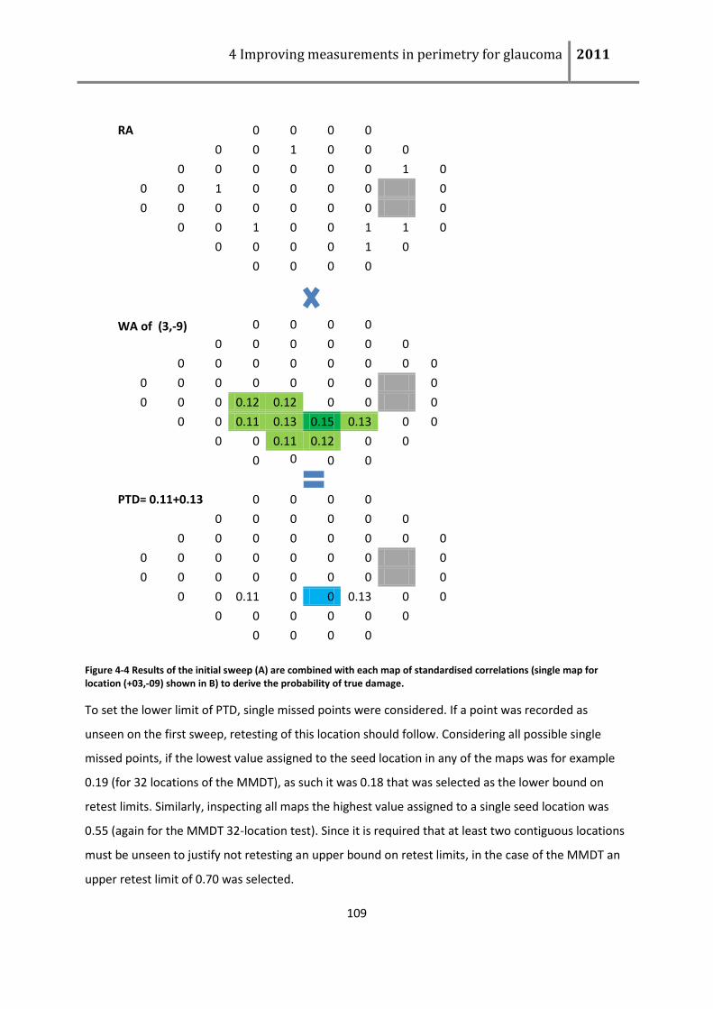
4 Improving measurements in perimetry for glaucoma 2011
109
Figure 4-4 Results of the initial sweep (A) are combined with each map of standardised correlations (single map for location (+03,-09) shown in B) to derive the probability of true damage.
To set the lower limit of PTD, single missed points were considered. If a point was recorded as
unseen on the first sweep, retesting of this location should follow. Considering all possible single
missed points, if the lowest value assigned to the seed location in any of the maps was for example
0.19 (for 32 locations of the MMDT), as such it was 0.18 that was selected as the lower bound on
retest limits. Similarly, inspecting all maps the highest value assigned to a single seed location was
0.55 (again for the MMDT 32-location test). Since it is required that at least two contiguous locations
must be unseen to justify not retesting an upper bound on retest limits, in the case of the MMDT an
upper retest limit of 0.70 was selected.
RA 0 0 0 0
0 0 1 0 0 0
0 0 0 0 0 0 1 0
0 0 1 0 0 0 0 0
0 0 0 0 0 0 0 0
0 0 1 0 0 1 1 0
0 0 0 0 1 0
0 0 0 0
WA of (3,-9) 0 0 0 0
0 0 0 0 0 0
0 0 0 0 0 0 0 0
0 0 0 0 0 0 0 0
0 0 0 0.12 0.12 0 0 0
0 0 0.11 0.13 0.15 0.13 0 0
0 0 0.11 0.12 0 0
0 0 0 0
PTD= 0.11+0.13 0 0 0 0
0 0 0 0 0 0
0 0 0 0 0 0 0 0
0 0 0 0 0 0 0 0
0 0 0 0 0 0 0 0
0 0 0.11 0 0 0.13 0 0
0 0 0 0 0 0
0 0 0 0
4 Improving measurements in perimetry for glaucoma 2011
110
With those points needing retesting now isolated we begin the second sweep. The intensity level can
be adjusted at this stage to increase specificity. For example testing twice at the 80% level of
normality would still equate to a 4% chance of missing a second presentation, in an average normal
observer. Considering that 32 or 52 locations are being tested in the above description, between 1
and 3 locations can reasonably be expected to return a defective result, which would increase as the
normal observer moved towards the upper centiles of the normative distribution. However,
increasing to an intensity level corresponding to the 95% limit would reduce this to less than 1
missed location in the average normal test subject.
At the locations which have been retested, ESTA uses the 2/3 Henson Pass/Fail criterion, therefore
to fail this test two points at or over the 95% limit level must be unseen for this location to be
classified as ‘defective’. Following the second sweep, the result array is updated and the PTD
recalculated for every location including those that were eliminated on the first sweep. Reapplying
the limits of acceptability, we isolate those test locations with ambiguous PTD values. These test
locations undergo a third iterative sweep. The results array (RA) is updated with the quotient of the
number of seen presentations and the total number of presentations at that location.
Following the third sweep the PTD is again recalculated. In a few cases there may be a fourth sweep
to satisfy the terminating criterion. After the test terminates the PTD is calculated again based on the
final results.
In short, each location will pass or fail the test based on two criteria:
The likelihood of a defect is either below 0.19 or above 0.7
Two presentations above the 95% have been missed by the observer
Generalising this, the ESTA algorithm begins with the simple ST strategy. Each TL is tested once with a
stimulus set at a fixed intensity level (this is an estimated threshold for the TL that would be seen in
95% of visually healthy subjects). Then each location has a recorded value of seen (beta) or unseen
(1-beta) in a results array (RA). For the purpose of this explanation beta will be taken as one, so seen
= 0 and unseen =1. In practice, the probability of the stimuli being seen at a fixed level (0.95) is
entered for a seen location and 0.05 for an unseen location (see appendix). This concludes the first
sweep or cycle of testing. Simultaneously, for each TL the WA and RA are convolved (see appendix).
This gives a value at each TL which represents the probability of the point being a glaucomatous
4 Improving measurements in perimetry for glaucoma 2011
111
defect dependent on the responses at TLs in the cluster of points that are considered to be
physiologically contiguous. For example, points missed in isolation are given a low so-called,
‘probability of true damage’ (PTD) whereas those close to, or at the edge of ‘physiologically likely’
clusters of defective points are given higher PTD.
∑
ESTA proceeds, in a novel fashion, to only examine those points without either a very high or very
low PTD. Thus, locations that have a high estimated PTD (above a first limit, U1) and those locations
that have a low estimated PTD (below a second limit, U2) are not selected for retesting. The only
locations selected for retesting have a value such that U1>PTD>U2. If no locations satisfy this
criterion, then the test terminates (see Figure 4-1). A stimulus is presented at a new intensity level
(see appendix) only at those locations selected by the algorithm for retesting. This concludes the
second sweep of testing.
The new (retest) results are recorded and combined with the previous results (see appendix) to
produce an updated version of the RA, and from that an updated set of estimated PTD values. These
estimated PTD values are now re-examined as before with locations selected for retesting by having
a value of PTD such that T1>PTD>T2 (where T1 is a lower arbitrary retest limit and T2 the upper
retest limit) and do not have two or more presentations giving the same result, i.e. both seen or both
unseen. A decision rule on the number of sweeps is now applied and if this is not satisfied a new
sweep of testing, using a stimuli set at a slightly different intensity, is carried out. One such set of
decision rules and termination criteria are given in the appendix. At the conclusion of the test each TL
has an estimated level of PTD. TLs that have an estimated PTD estimated above the associated upper
bound (>T1) are flagged, using standard ST terminology, as failed, and all other TLS are considered to
have passed the test. Each point has a PTD value and a simple summary measure of these values is
the sum of all PTD values. This gives a global index of VF loss as, for example, a mean deviation (MD)
measure in Humphrey SAP.
ESTA for the MMDT (Appendix- Matlab code of ESTA) was first developed in Matlab (version
7.2.0.232 (R2006a)) and then directly programmed into the MMDT software, and details of the ESTA
program as implemented with the official version of the MMDT are given in Appendix A. Other ST
testing is also available on the research version of the software.
4 Improving measurements in perimetry for glaucoma 2011
112
4.2 Patient data approach
The cohort of subjects described in chapter two and three all underwent suprathreshold testing. This
data was collected on a different and subsequent day to FOS data collection. Data were collected
equally by CB and RM. Fourteen patients with a clinical diagnosis of primary open angle glaucoma in
at least one eye were recruited from Moorfields Eye Hospital, London. Patients were purposely
selected to give a range of VF defect severity. All were experienced in SAP and had prior experience
with MMDT.
Inclusion and exclusion criteria for the healthy observers and the glaucoma patients recruited for this
study were as described in section 2.3.1. The study was approved by the Moorfields Ethics
Committee and conformed to the Declaration of Helsinki with all participants giving their informed
written consent.
4.2.1 Methods
For each participant in this study we needed to determine a ‘ground truth’ on whether a TL was
‘abnormal or ‘normal’. To do this we devised a surrogate value from the threshold testing conducted
in Chapter 3. From Moosavi and colleagues, the 95th centile normal limit of threshold was defined
(Moosavi, In submission; MD Thesis). Results of four threshold search trials collected from this cohort
were available. Examining threshold estimates at each location allowed a classification of whether a
location was within or outside normal limits. If the result of two or more trials returned threshold
estimations above the 95th centile then this test location was classified as outside normal limits
(criterion 1). An alternative stricter criterion was also examined: if a test location was classified as
outside normal limits on 3 or more of the threshold estimation examinations, this test location was
classified as outside normal limits (criterion 2).
For suprathreshold estimation, the test subjects (visually healthy and glaucomatous patients)
described in chapter two and three underwent an additional component during their second visit. In
addition, during the second visit, subsequent to threshold examination described in chapter 3, each
participant underwent MMDT testing with a customised ST tests strategy. During the ST strategy
each location was tested three times, such that each TL had 3 trials performed in randomised order.
4 Improving measurements in perimetry for glaucoma 2011
113
From this data C 1/2, MS 1/2 and MS 2/3 test outcomes were calculated. Each participant also
underwent ESTA suprathreshold test separately. The order in which the ST and ESTA strategies were
performed was randomised.
Each TL, in both the ST strategy and the ESTA strategy was examined in random order with a
displacement equivalent to that expected to be seen in an estimated 95th centile of visually healthy
subjects. These values were the current machine norms, being derived from a study of 120 visually
healthy subjects, where thresholds were established using a staircase algorithm (Moosavi, In
submission; MD Thesis).
The agreement and associated concordant/discordant pairs for each suprathreshold method against
criterion 1 (Table 4-1) and criterion 2 (Table 4-2) were examined. The overall agreement as defined
by Eqn 4-2 was also calculated, with the associated confidence limits.
Equation 4-2
4.2.2 Results
Figure 4-5 shows the summary of test duration for each of the suprathreshold methods. C1/2
suprathreshold method had shorter test duration than any other methodology. ESTA showed an
overall average increase of 17% (SD =17%, range = -7% to 73%) in test duration over C 1/2, being
broken down as a 12% increase for visually healthy eyes (SD=9%, range = 3% to 32%) and 21% for
glaucomatous eyes (std =22%, range = -7% to 73%). The increase in number of required
presentations for visually healthy and glaucomatous patients was significant (p=0.002 and P<0.001
respectively; two sample t-test). ESTA required significantly less presentations than MS 1/2 or MS 2/3
(p<0.0001 for all groups and subgroups, two sample t-test). MS 1/2 took 51% longer than ESTA (SD
=22%, range 8% to 85%), while MS 2/3 took 69% longer than ESTA (SD 22%, range 14% to 100%).
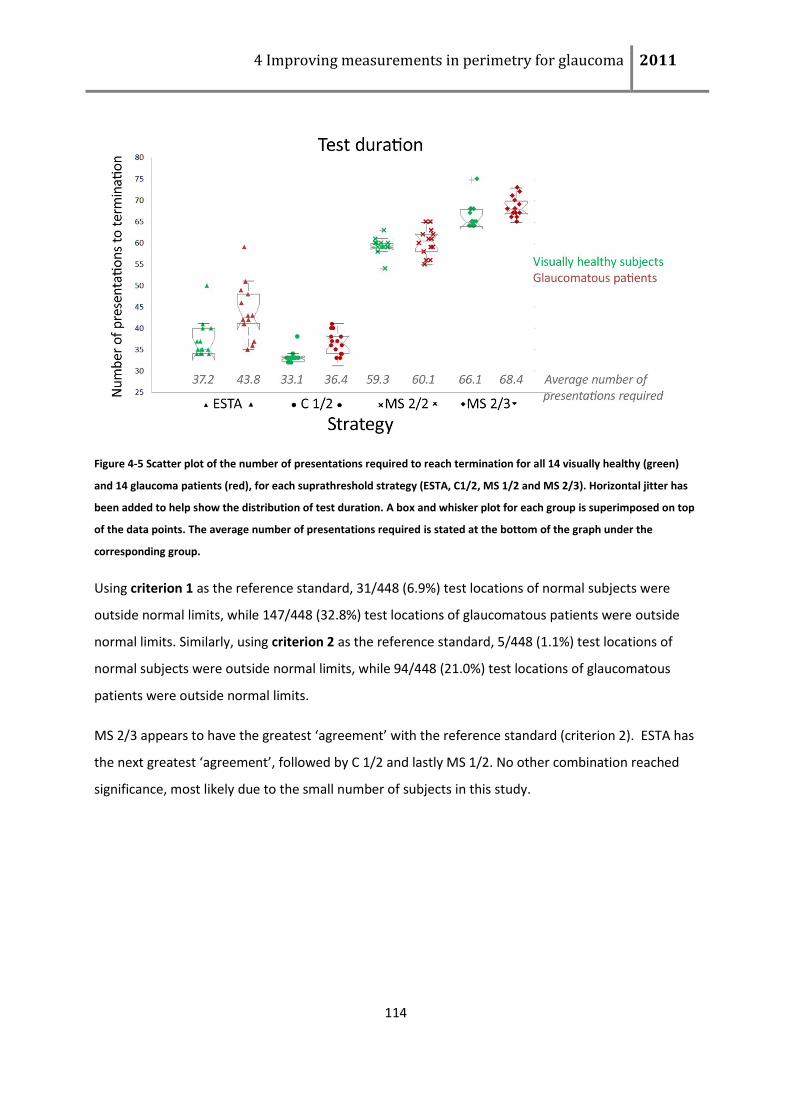
4 Improving measurements in perimetry for glaucoma 2011
114
Figure 4-5 Scatter plot of the number of presentations required to reach termination for all 14 visually healthy (green)
and 14 glaucoma patients (red), for each suprathreshold strategy (ESTA, C1/2, MS 1/2 and MS 2/3). Horizontal jitter has
been added to help show the distribution of test duration. A box and whisker plot for each group is superimposed on top
of the data points. The average number of presentations required is stated at the bottom of the graph under the
corresponding group.
Using criterion 1 as the reference standard, 31/448 (6.9%) test locations of normal subjects were
outside normal limits, while 147/448 (32.8%) test locations of glaucomatous patients were outside
normal limits. Similarly, using criterion 2 as the reference standard, 5/448 (1.1%) test locations of
normal subjects were outside normal limits, while 94/448 (21.0%) test locations of glaucomatous
patients were outside normal limits.
MS 2/3 appears to have the greatest ‘agreement’ with the reference standard (criterion 2). ESTA has
the next greatest ‘agreement’, followed by C 1/2 and lastly MS 1/2. No other combination reached
significance, most likely due to the small number of subjects in this study.
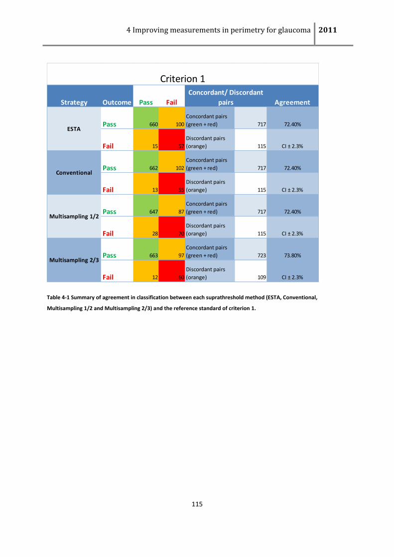
4 Improving measurements in perimetry for glaucoma 2011
115
Table 4-1 Summary of agreement in classification between each suprathreshold method (ESTA, Conventional,
Multisampling 1/2 and Multisampling 2/3) and the reference standard of criterion 1.
Strategy Outcome Pass Fail Agreement
Pass 660 100
Concordant pairs
(green + red) 717 72.40%
Fail 15 57
Discordant pairs
(orange) 115 CI ± 2.3%
Pass 662 102
Concordant pairs
(green + red) 717 72.40%
Fail 13 55
Discordant pairs
(orange) 115 CI ± 2.3%
Pass 647 87
Concordant pairs
(green + red) 717 72.40%
Fail 28 70
Discordant pairs
(orange) 115 CI ± 2.3%
Pass 663 97
Concordant pairs
(green + red) 723 73.80%
Fail 12 60
Discordant pairs
(orange) 109 CI ± 2.3%
Multisampling 2/3
Criterion 1Concordant/ Discordant
pairs
ESTA
Conventional
Multisampling 1/2
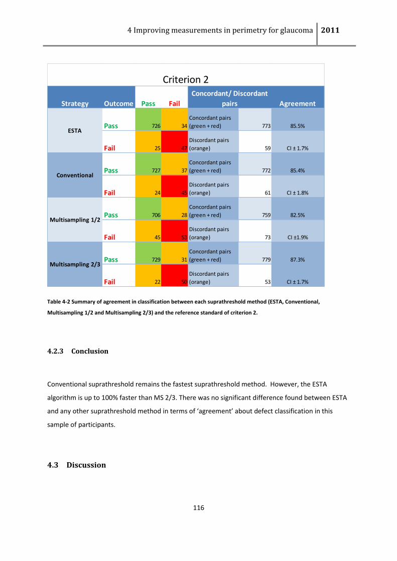
4 Improving measurements in perimetry for glaucoma 2011
116
Table 4-2 Summary of agreement in classification between each suprathreshold method (ESTA, Conventional,
Multisampling 1/2 and Multisampling 2/3) and the reference standard of criterion 2.
4.2.3 Conclusion
Conventional suprathreshold remains the fastest suprathreshold method. However, the ESTA
algorithm is up to 100% faster than MS 2/3. There was no significant difference found between ESTA
and any other suprathreshold method in terms of ‘agreement’ about defect classification in this
sample of participants.
4.3 Discussion
Strategy Outcome Pass Fail Agreement
Pass 726 34
Concordant pairs
(green + red) 773 85.5%
Fail 25 47
Discordant pairs
(orange) 59 CI ± 1.7%
Pass 727 37
Concordant pairs
(green + red) 772 85.4%
Fail 24 45
Discordant pairs
(orange) 61 CI ± 1.8%
Pass 706 28
Concordant pairs
(green + red) 759 82.5%
Fail 45 53
Discordant pairs
(orange) 73 CI ±1.9%
Pass 729 31
Concordant pairs
(green + red) 779 87.3%
Fail 22 50
Discordant pairs
(orange) 53 CI ± 1.7%
Multisampling 2/3
Criterion 2Concordant/ Discordant
pairs
ESTA
Conventional
Multisampling 1/2
4 Improving measurements in perimetry for glaucoma 2011
117
The data presented here is derived from a small sample of glaucomatous patients and visually
healthy subjects and as such may not be representative of the general population or, indeed, of the
glaucomatous patient population. However, this data demonstrates that ESTA performs to the
conventional suprathreshold methods in terms of ‘agreement' against a surrogate reference
standard determined from threshold testing. ESTA seems quicker than the multi-sampling
approaches described by Artes et al (Artes et al., 2003) but doesn’t appear to lose diagnostic
accuracy.
Time saving is important in the context of getting more reliable perimetric results. According to
Henson and Emuh the time between test onset and enlarged amplitude of the ‘fatigue wave’ is less
than three minutes (Henson and Emuh, 2010). After three minutes the mid amplitude ‘fatigue wave’
can occur, which is associated with a 20% decrease in probability of seeing from 90% to 70% at 3dB
above reference threshold. This shift in the FOS curve is associated with an ‘increase in amplitude of
fatigue waves’. In some cases of visually healthy subjects this manifests as an apparent increase in
lapse rate and corresponds to an increase in unseen presentations. In a suprathreshold test of
visually healthy subject the lapse rate is proportional to the number of locations flagged as
‘defective’. A quicker test will help keep ‘fatigue’ within acceptable limits, thus helping to maintain a
low number of ‘defective’ locations in visually healthy naïve subjects.
A higher presentation intensity level will be more robust to the fatigue effect described by Henson
and Emuh (2009). However, the ideal presentation intensity level is not obvious. In strategies like
that of the HEART algorithm, where the local normative value is estimated and a higher intensity
level (5dB above threshold) is used (Henson and Artes, 2002) the shift in the underlying FOS curve
associated with the ‘fatigue wave’ is likely to have a greater impact on the number of visually healthy
subjects flagged as ‘abnormal’ than on those where the presentation intensity level is set at a
predefined level from the normative database.
Full field simulation (FFS) becomes particularly difficult when spatial information is being used. If a
new test algorithm exploits the spatial connectivity of the retinal sensitivity values, then testing it on
a patient simulator that doesn’t incorporate the same information will, by experimental design, lead
to incongruous results. At the same time if both incorporate the same spatial information then the
results are likely to be unrealistic. To implement a FFS accurately, full field FOS data would be
required, since this is not available the ORS approach with a full field simulation implemented was
not attempted within this chapter.
4 Improving measurements in perimetry for glaucoma 2011
118
Theoretically, the more information gathered on each location the better the probability of correctly
labelling a location as ‘non- defective’ or ‘defective’ (Artes et al., 2003). Since the FOS curve changes
considerably with increased test duration, there is an argument that collecting more information in
suprathreshold testing weakens the ability of the test to correctly classify ‘normal’ and ‘abnormal’.
Using the spatial information incorporated in the ESTA algorithm, may allow isolation of the test
locations where further information is required, while minimally increasing test duration.
It is clear that there is a delicate balance between time and accuracy, and this depends on the testing
scenario. In the screening or case detection scenario, test duration is paramount to maintain both
accuracy of suprathreshold test and acceptability of the test for the patient and operator. Put in
context, a suprathreshold test such as ESTA, takes a little over one quarter of the time that a
threshold test takes. It is accepted clinical practice that perimetric exams utilising threshold search
methods are more suitable for secondary or tertiary care, where both the depth and the size of the
VF defects are monitored. However, it is clear that in the screening or case finding scenario, the
suprathreshold strategy has many advantages, for example, test results are easily interpretable and
the test has high presentation intensity levels with short test duration. Combined these make
suprathreshold testing more suitable for the naïve test subject. However, one question remains:
does the threshold search method have greater diagnostic accuracy? In section 5.5, this question is
revisited.
5 Using the new test algorithms (ESTA and WEBS)
One of the main outcomes from the work described in this thesis has been the development of novel
perimetry test algorithms. To recap, one of these methods is designed to provide a rapid test to be
used in screening and case finding (ESTA), whilst the other (WEBS, specifically designed for the
MMDT) is intended for measuring the severity of impairment to a displacement stimuli at the
different locations in the visual field, thus being equivalent to a ‘threshold’ test. This chapter first
briefly describes interim results from a multi-centre prospective trial (started in 2009) designed to
compare the performance of the MMDT, using the algorithms (ESTA and WEBS) as developed in this
thesis, against other perimetric instruments (This will be referred to as the The Perimetry Instrument
Comparison Study). A summary of this study will be given in section 5.1. The work reported in other
parts of the chapter (sections 5.2 and 5.3) formed two posters presented at the Association for
Research in Vision and Ophthalmology Meeting, Fort Lauderdale, Florida, USA in May 2010 ((Bergin
et al., 2010a, Sinapis et al., 2010); see ‘List of supporting publications’). The joint authors of this work
are Ciara Bergin [CB], Dimitrios Sinapis [DS], Angelos Sinapis [AS], Reza Moosavi [RM], Gay Verdon-
Roe [GVR], Richard Russell [RR], David Crabb [DC] and David Garway-Heath [DGH]. The study was
conceived and designed by DGH, GVR with help from DC. The prospective data was collected from
patients attending Moorfields Eye Hospital by DS, AS and RM. Other centres in Italy and Canada were
involved in data collection (see below). Extensive data management across all centres was performed
and co-ordinated by CB with help from GVR. All the data and graphical analyses, along with
development and conception of quantitative techniques, were performed by CB with some help from
RR. One of the posters was wholly written and first authored by CB (Bergin et al. 2010a) with all other
authors contributing in part. All the work was supervised by DGH and DC. The final study results are
due to be reported in 2012. The work reported towards the end of the chapter (section 5.5) formed a
read paper presentation at the 19th International Symposium of the Imaging and Perimetry Society
Meeting in Tenerife, Spain in May 2010 ((Bergin et al., 2010b); See ‘List of supporting publications’).
The joint authors of this work are Ciara Bergin [CB], Gay Verdon-Roe [GVR], Eamon Sharkawi [ES],
David Crabb [DC] and David Garway-Heath [DGH]. The study was conceived and designed by ES.
Subject testing and data collection was, in part, done by CB along with other workers at Hôpital
Ophthalmique Jules-Gonin, Lausanne, Switzerland. Data analysis was performed by CB. The
presentation was first authored by CB with all other authors contributing in part.
5 Improving measurements in perimetry for glaucoma 2011
120
5.1 The perimetry instrument comparison study
This study was conducted a four centres: Moorfields Eye Hospital, London, UK; Bietti Foundation,
Rome, Italy; Dalhousie University, Halifax, Nova Scotia, Canada; and Waterloo University, Toronto,
Canada. The study aimed to collect 160 visually healthy subjects and 160 glaucomatous patients.
There are different aspects to this study: relative comparative diagnostic accuracy of three different
perimeters with suprathreshold and four different perimeters with threshold testing strategies, and
comparing the repeatability of these perimeters in threshold estimation. The overall study did not
aim to assess the performance of the devices in routine clinical use. The index tests are all the
different perimeters investigated in the study. In this way, the index tests (the different perimetric
instruments) may be compared with each other and against a common reference standard. The
reference standard is not taken as the ‘gold standard’ (as there is no gold standard for the diagnosis
of glaucoma), so that the diagnostic accuracies determined in this study are relative, not absolute.
The primary research objective of the The Perimetry Instrument Comparison Study (PICS) is to
compare the sensitivity of the Humphrey visual field perimeter, Frequency Doubling Technology,
Moorfields Motion Displacement Test (SAP, FDT, and MMDT respectively) and The Heidelberg Edge
Perimeter (HEP using FDF perimetry) to detect glaucomatous RNFL loss. The study followed the
guidelines of the STARD steering committee (Standards for Reporting of Diagnostic Accuracy)
http://www.stard-statement.org/ (Bossuyt et al., 2003a, Bossuyt et al., 2003b). The design of the
experiment and sample calculations was primarily based on examining the performance of the
different instruments in terms of sensitivity of each device at a fixed specificity of 95%. The study is
powered (n=320) to give a 95% confidence interval (CI) of 90.4 to 97.4% for this fixed specificity
(95%).
All subjects underwent HRT imaging and IOP assessment (GAT). Visually healthy subjects were
required to be “within normal limits” on the global and each sector of the Moorfields Classification
with IOP≤21mmHg. Glaucomatous patients were classified based as those subjects “Outside normal
limits” for at least one sector of the Moorfields Classification with IOP>21mmHg at least once during
follow-up before treatment, but not during the PICS data collection period. It was also required that
both cohorts have no history of ocular surgery (apart from uncomplicated phacoemulsification) or
other ocular pathology (eg cataract) or systemic disease which may affect visual performance. Prior
5 Improving measurements in perimetry for glaucoma 2011
121
to participation all subjects provided written informed consent in accordance with a protocol
approved by NHS foundation trust, and in accordance to the tenets of the Declaration of Helsinki.
5.2 Comparing the ‘screening’ strategies of three perimetry devices to
discriminate between healthy and ‘glaucomatous’ eyes (interim results)
5.2.1 Background and purpose
Screening or case-finding perimetric tests demand higher specificity and shorter test duration than
those in secondary or tertiary care, making suprathreshold testing a favoured choice. Furthermore,
the ease of understanding and lower fatigue effect associated with ST tests is of added benefit in
naïve subjects. A comprehensive review of the published literature pertaining to screening tools for
glaucoma, including standard and newer types of perimetric devices, indicated that the FDT1 was a
perimetric device with potential as a glaucoma screening tool (Mowatt et al., 2008). MMDT and FDF,
however, were not included in that meta-analysis because these devices are not currently
commercially available. SAP was included in the meta-analysis, as both a threshold test and a
suprathreshold test.
There were three perimetric instruments involved in this aspect of the perimetry comparison study,
namely namely FDT1 (see section 1.7.3.2), MMDT (see section 1.7.3.3) and SAP (see section 1.7.2).
The FDF screening test was still in development at the start point of this study.
The FDT1 was selected over the FDT MATRIX as the screening tool, as it is reportedly the more widely
used clinical tool in the UK (Myint et al., 2010, Myint et al., 2011). The format of the FDT1 C-20 test is
of 17 test locations (see Figure 1-7 (C)). To the best of our knowledge details of the test strategy are
not published. The C-20 format was selected as it was previously reported to have good
discriminatory power (Cioffi et al., 2000, Nehmad and Madonna, 2008, Zwarts and Stoutenbeek,
2010), with low learning and fatigue effects (Brush and Chen, 2004), and has been included in several
comparative studies previously (De Tarso Ponte Pierre Filho et al., 2006, Iester et al., 2000).
Approximately 20% of eyes fail the initial test and repeat testing has been recommended to increase
specificity (Mansberger et al., 2007).
5 Improving measurements in perimetry for glaucoma 2011
122
The MMDT 32-location format (see Figure 1-8 (B)) using the ESTA strategy (see section 4.1) was
selected. This strategy had undergone the pilot study outlined in section 4.2, and also been included
in a multi-instrument screening scenario in St. Kitts (Artes et al., 2009), where it reportedly had
higher sensitivity than FDT MATRIX 24-2-1 and SAP 76-point screen 3 zone test at fixed levels of
specificity.
The SAP 64-point screener test format (see 1-5 (C)) with the C1/2 suprathreshold test is outlined in
chapter 4. According to the manufacturers’ guidelines it is the standard screening ST test available on
the HFA instrument (personal communication: John Hood October 2009). Suprathreshold testing in
the HFA device have been largely neglected with little or no development in recent years.
The aim of this aspect of the study was to consider interim study results of the relative diagnostic
precision and test duration of the screening strategies of three perimetry devices (including MMDT
using ESTA) to discriminate between healthy and ‘glaucomatous’ eyes, defined by neuroretinal rim
loss and intraocular pressure (IOP) level (Bergin et al., 2010a).
5.2.2 Methods
The results from the first test session were examined. Visually healthy subjects and glaucomatous
subjects were defined as outlined in section 5.1. One eye from each subject was selected for
inclusion in the study; if both eyes met the study criteria then one eye was selected randomly. The
order of the instruments was randomised between test subjects. Each subject underwent the
training demonstration program for each instrument. If the reliability indices did not meet the
criteria (SAP (FP<15%, FN<15%); FDT (FP<15%, FN<15%); MMDT (FP<15%)), the suprathreshold
program was repeated once. If on repeat test results were not within the criteria specified, the
subject was excluded from further testing and all data from this subject were excluded from analysis.
5.2.3 Results
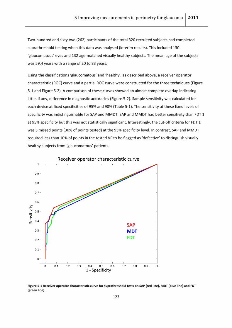
5 Improving measurements in perimetry for glaucoma 2011
123
Two-hundred and sixty two (262) participants of the total 320 recruited subjects had completed
suprathreshold testing when this data was analysed (interim results). This included 130
‘glaucomatous’ eyes and 132 age-matched visually healthy subjects. The mean age of the subjects
was 59.4 years with a range of 20 to 83 years.
Using the classifications ‘glaucomatous’ and ‘healthy’, as described above, a receiver operator
characteristic (ROC) curve and a partial ROC curve were constructed for the three techniques (Figure
5-1 and Figure 5-2). A comparison of these curves showed an almost complete overlap indicating
little, if any, difference in diagnostic accuracies (Figure 5-2). Sample sensitivity was calculated for
each device at fixed specificities of 95% and 90% (Table 5-1). The sensitivity at these fixed levels of
specificity was indistinguishable for SAP and MMDT. SAP and MMDT had better sensitivity than FDT 1
at 95% specificity but this was not statistically significant. Interestingly, the cut-off criteria for FDT 1
was 5 missed points (30% of points tested) at the 95% specificity level. In contrast, SAP and MMDT
required less than 10% of points in the tested VF to be flagged as ‘defective’ to distinguish visually
healthy subjects from ‘glaucomatous’ patients.
Figure 5-1 Receiver operator characteristic curve for suprathreshold tests on SAP (red line), MDT (blue line) and FDT (green line).
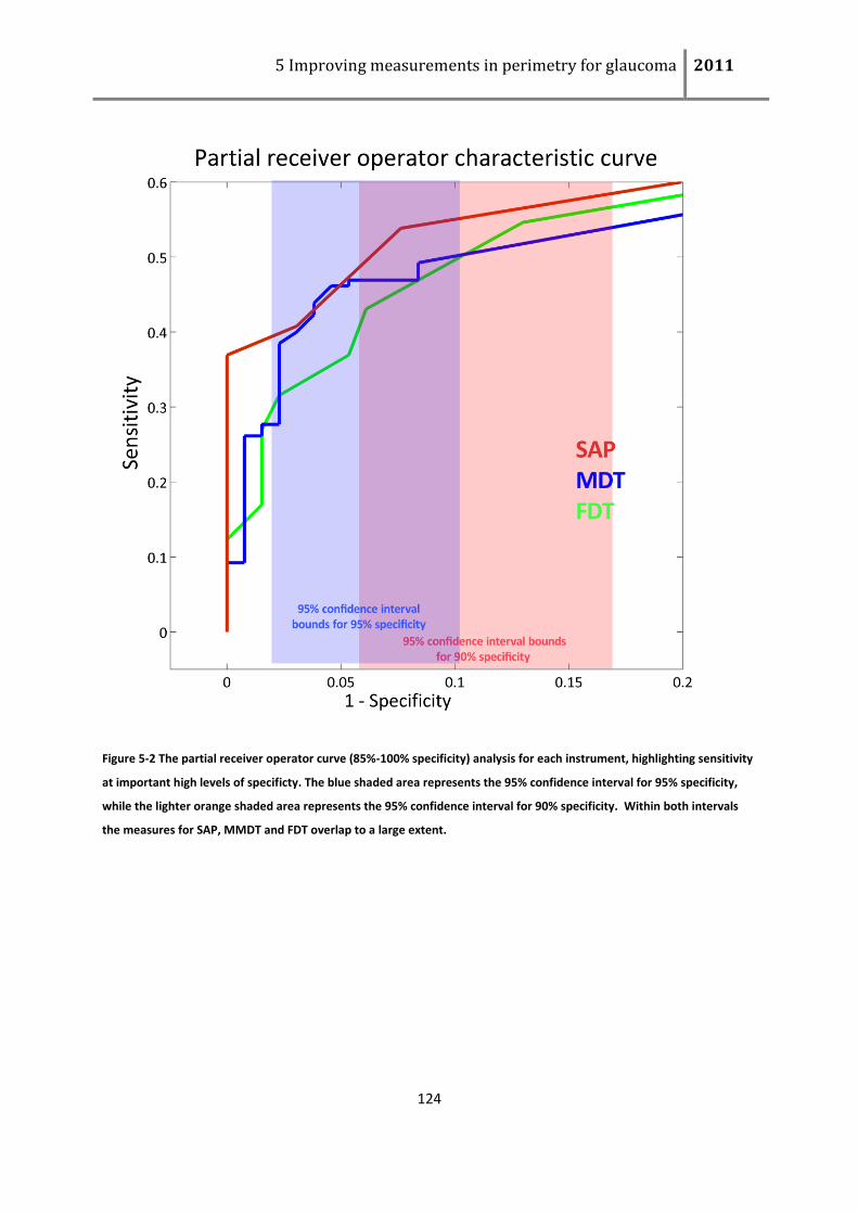
5 Improving measurements in perimetry for glaucoma 2011
124
Figure 5-2 The partial receiver operator curve (85%-100% specificity) analysis for each instrument, highlighting sensitivity
at important high levels of specificty. The blue shaded area represents the 95% confidence interval for 95% specificity,
while the lighter orange shaded area represents the 95% confidence interval for 90% specificity. Within both intervals
the measures for SAP, MMDT and FDT overlap to a large extent.
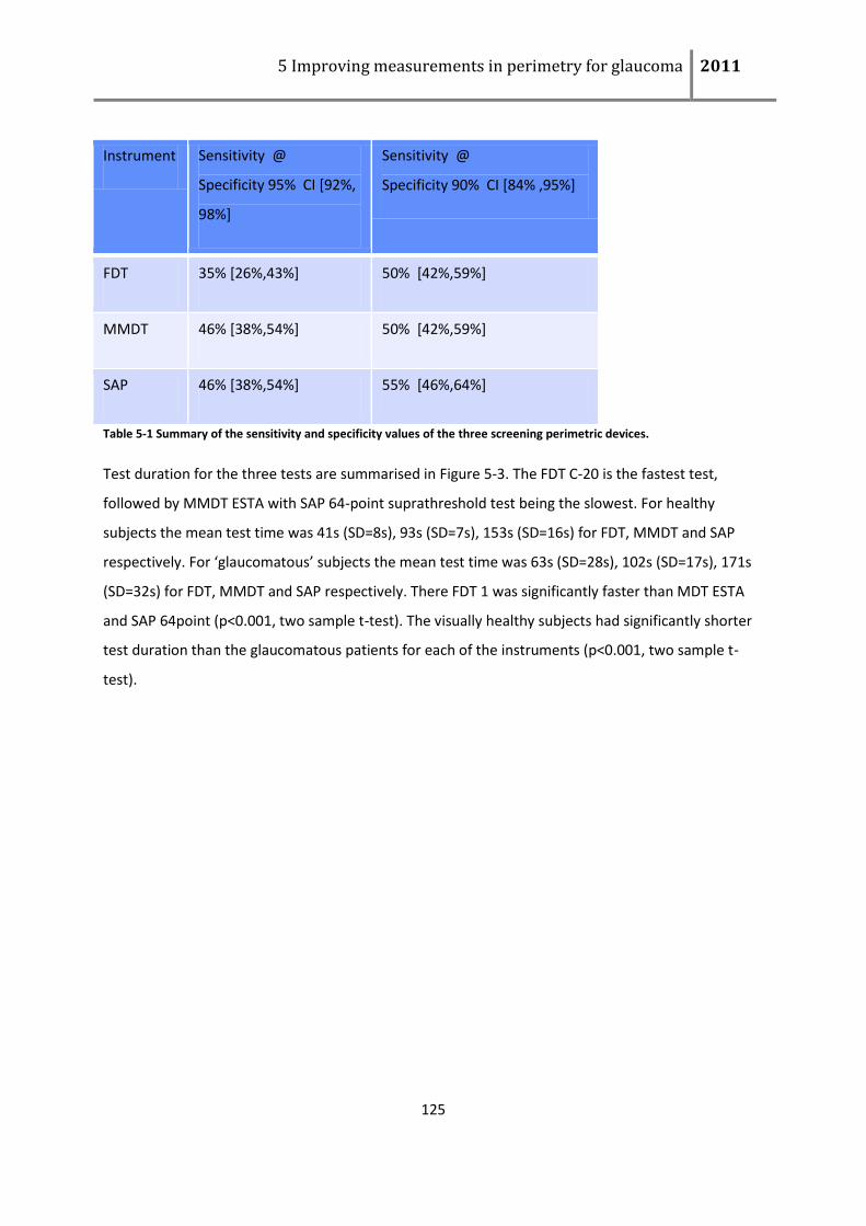
5 Improving measurements in perimetry for glaucoma 2011
125
Instrument Sensitivity @
Specificity 95% CI [92%,
98%]
Sensitivity @
Specificity 90% CI [84% ,95%]
FDT 35% [26%,43%] 50% [42%,59%]
MMDT 46% [38%,54%] 50% [42%,59%]
SAP 46% [38%,54%] 55% [46%,64%]
Table 5-1 Summary of the sensitivity and specificity values of the three screening perimetric devices.
Test duration for the three tests are summarised in Figure 5-3. The FDT C-20 is the fastest test,
followed by MMDT ESTA with SAP 64-point suprathreshold test being the slowest. For healthy
subjects the mean test time was 41s (SD=8s), 93s (SD=7s), 153s (SD=16s) for FDT, MMDT and SAP
respectively. For ‘glaucomatous’ subjects the mean test time was 63s (SD=28s), 102s (SD=17s), 171s
(SD=32s) for FDT, MMDT and SAP respectively. There FDT 1 was significantly faster than MDT ESTA
and SAP 64point (p<0.001, two sample t-test). The visually healthy subjects had significantly shorter
test duration than the glaucomatous patients for each of the instruments (p<0.001, two sample t-
test).
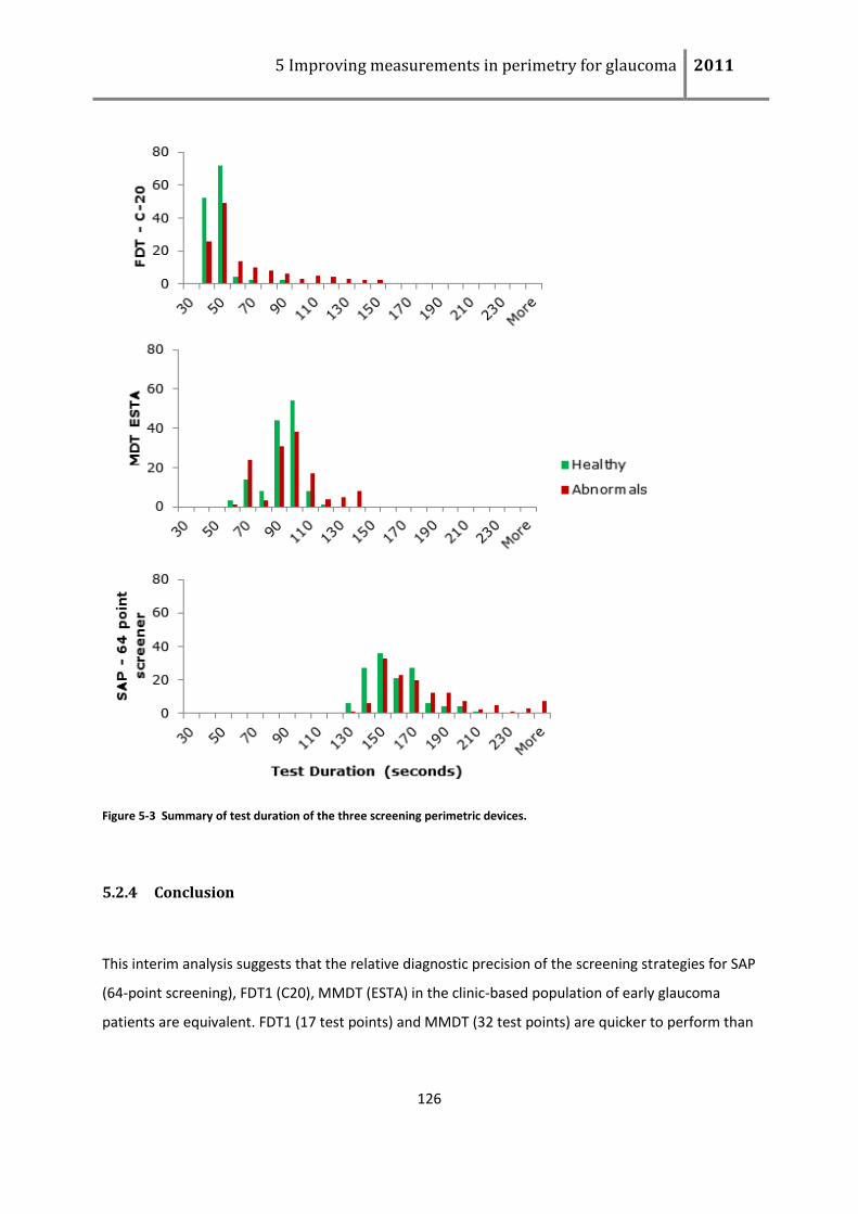
5 Improving measurements in perimetry for glaucoma 2011
126
Figure 5-3 Summary of test duration of the three screening perimetric devices.
5.2.4 Conclusion
This interim analysis suggests that the relative diagnostic precision of the screening strategies for SAP
(64-point screening), FDT1 (C20), MMDT (ESTA) in the clinic-based population of early glaucoma
patients are equivalent. FDT1 (17 test points) and MMDT (32 test points) are quicker to perform than
5 Improving measurements in perimetry for glaucoma 2011
127
the SAP screening strategy. It is most likely related to the number of test locations with the test
procedures having a lesser contribution.
The large proportion of ‘defective’ test locations isolated by the FDT1 C-20 in order to achieve similar
levels of specificity as MMDT and SAP, suggests that the referral criterion (2 ‘defective’ locations) is
not at present set to the correct level. This is likely to be a significant contributor to the large
proportion of tests failing the first screening (Mansberger et al., 2007). An adjustment to the referral
criterion may remove the need for repeat testing.
5.3 Comparing the diagnostic performance of four threshold perimetry tests to
discriminate between healthy and ‘glaucomatous’ eyes (interim analysis)
5.3.1 Background and purpose
Agreement between instruments and in particular agreement between structural and functional
measures aids clinical confirmation of glaucoma diagnosis and detection of glaucomatous
progression. In this part of the perimetric comparison study we are comparing the relative diagnostic
precision of each perimetric instrument, when diagnosis has been made independently of visual
function measures. There were four perimetric instruments involved in this aspect of the perimetry
comparison study, namely SAP (see section 1.7.2 ), FDT MATRIX (see section 1.7.3.2), HEP (with FDF
stimulus type; see section 1.7.3.4) and MMDT (see section Figure 1.7.3.3).
With SAP the standard 24-2 test pattern was selected (see Figure 1-5(B)). The SITA standard
threshold algorithm was used. This is the most commonly reported testing format in the literature,
therefore it is useful to continue to report on this format to allow comparison between this and
other previously reported studies. The agreement between SAP and structural measures has been
repeatedly examined; the outcomes have considerable variation dependent on disease severity of
the study population (Bowd et al., 2008, Bowd et al., 2006, Bowd et al., 2001, Bowd et al., 2000, Shah
et al., 2006).
5 Improving measurements in perimetry for glaucoma 2011
128
The FDT 24-2 test pattern (see Figure 1-7 (B)) with a ZEST algorithm (Anderson, 2003b, Anderson and
Johnson, 2006)(see section 3.2) was used. All threshold tests on the FDT MATRIX use the ZEST
algorithm (Zeppieri and Johnson, 2008). The 24-2 format closely matches the test format of the HFA
24-2 format, in terms of location placement, but it is not exact (see Figure 1-5 (B) and Figure 1-7 (B)).
In the literature this test format has been used previously to compare the diagnostic accuracy to that
of SAP SITA (Clement et al., 2009, Artes et al., 2005, Spry et al., 2005, Racette et al., 2008).
The test pattern on the HEP with the FDF stimulus type was also the 24-2. The test locations of this
format have been matched exactly to the stimulus locations reportedly used in the HFA SAP 24-2.
The so-called “Standard Adaptive Staircase Thresholding Algorithm” (ASTA-Std) has been
implemented on this instrument. There is no real detail about this algorithm in the literature and it
has simply been described as using up/down staircase procedure that is modified relative to the
expected normal database. This test format has recently been used to compare threshold and
deficits estimates of FDF to those of HFA SAP SITA (Calvo Perez et al., 2011, Gil, 2011).
The test format of the MMDT is different from the standard 52 point 24-2 test format. In this case a
subset, 32 of the 52 points, were selected for testing. These 32 test locations correspond directly to
32 of the 52 test locations tested in FDF and SAP. The test algorithm used in this scenario was WEBS
as documented in section 3.3.1. Until this time the multi-locational MMDT has not been included in
any large comparative studies.
The purpose of this aspect of the study was to consider interim results of the relative diagnostic
performance of four threshold tests, including MMDT using WEBS, to discriminate between healthy
and ‘glaucomatous’ eyes, defined by neuroretinal rim loss and intraocular pressure (IOP) level
(Sinapis et al., 2010).
5.3.2 Methods
For this aspect of the perimetry instrument comparison study, between the four test centres 274 of
the 320 test subjects were recruited and tested. Of these 136 were classified as ‘glaucomatous’
based on outside normal limits HRT MRA analysis and elevated IOP (>21mmHg), while 138 age
matched healthy controls were also examined. Test subjects were divided into visually healthy
(green) and ‘glaucomatous’ patients (orange) based on OHN appearance and IOP.
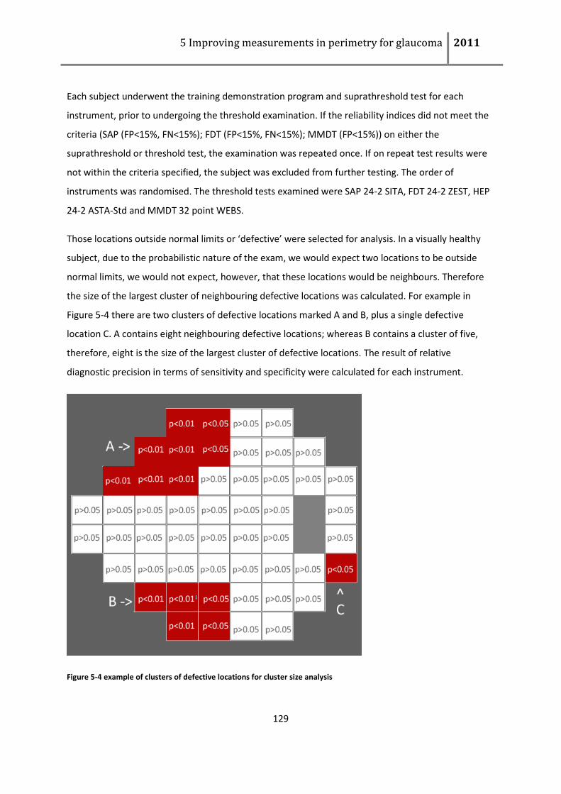
5 Improving measurements in perimetry for glaucoma 2011
129
Each subject underwent the training demonstration program and suprathreshold test for each
instrument, prior to undergoing the threshold examination. If the reliability indices did not meet the
criteria (SAP (FP<15%, FN<15%); FDT (FP<15%, FN<15%); MMDT (FP<15%)) on either the
suprathreshold or threshold test, the examination was repeated once. If on repeat test results were
not within the criteria specified, the subject was excluded from further testing. The order of
instruments was randomised. The threshold tests examined were SAP 24-2 SITA, FDT 24-2 ZEST, HEP
24-2 ASTA-Std and MMDT 32 point WEBS.
Those locations outside normal limits or ‘defective’ were selected for analysis. In a visually healthy
subject, due to the probabilistic nature of the exam, we would expect two locations to be outside
normal limits, we would not expect, however, that these locations would be neighbours. Therefore
the size of the largest cluster of neighbouring defective locations was calculated. For example in
Figure 5-4 there are two clusters of defective locations marked A and B, plus a single defective
location C. A contains eight neighbouring defective locations; whereas B contains a cluster of five,
therefore, eight is the size of the largest cluster of defective locations. The result of relative
diagnostic precision in terms of sensitivity and specificity were calculated for each instrument.
Figure 5-4 example of clusters of defective locations for cluster size analysis
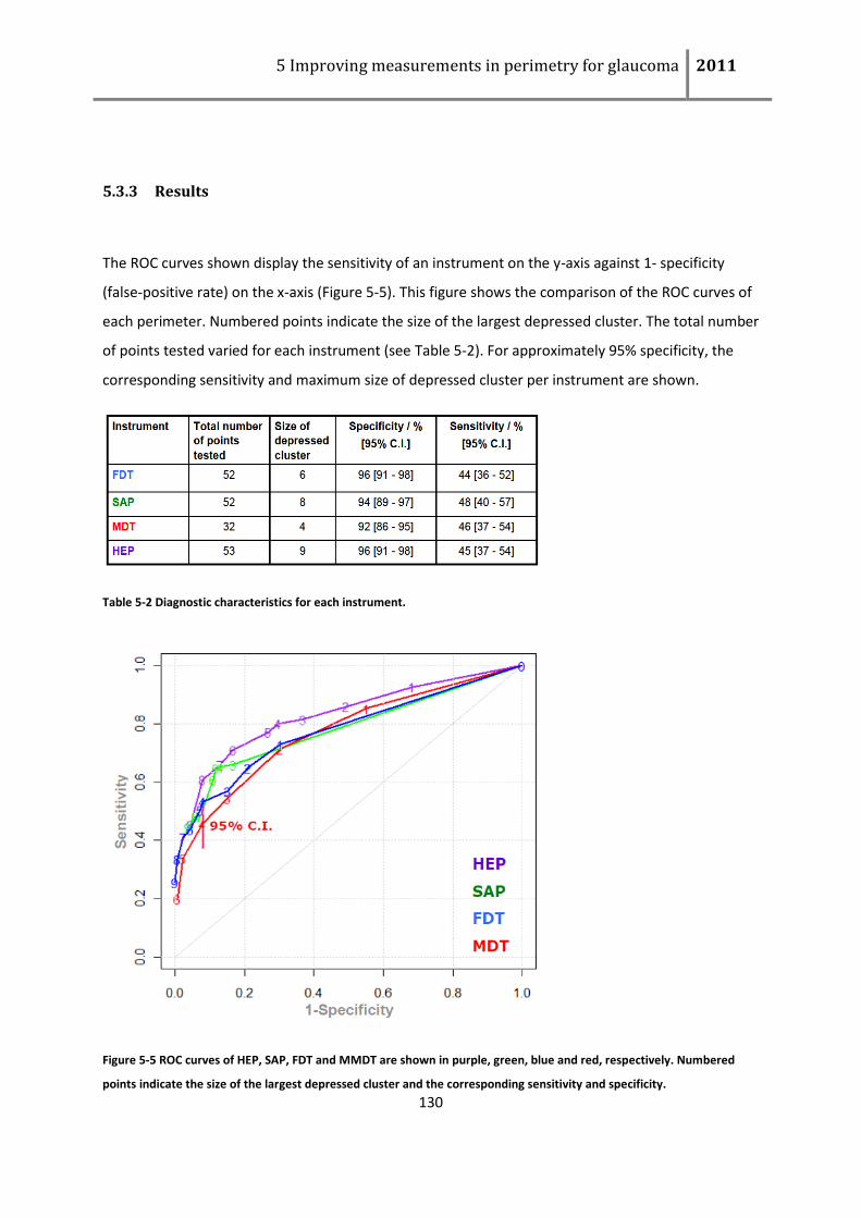
5 Improving measurements in perimetry for glaucoma 2011
130
5.3.3 Results
The ROC curves shown display the sensitivity of an instrument on the y-axis against 1- specificity
(false-positive rate) on the x-axis (Figure 5-5). This figure shows the comparison of the ROC curves of
each perimeter. Numbered points indicate the size of the largest depressed cluster. The total number
of points tested varied for each instrument (see Table 5-2). For approximately 95% specificity, the
corresponding sensitivity and maximum size of depressed cluster per instrument are shown.
Table 5-2 Diagnostic characteristics for each instrument.
Figure 5-5 ROC curves of HEP, SAP, FDT and MMDT are shown in purple, green, blue and red, respectively. Numbered
points indicate the size of the largest depressed cluster and the corresponding sensitivity and specificity.
5 Improving measurements in perimetry for glaucoma 2011
131
5.3.4 Conclusion
Diagnostic precision as estimated by ROC analysis suggest there is little difference between the perimeters,
there was no significant difference in the sensitivities of all four perimetry instruments at 95% specificity. Since
patients with early glaucoma were tested, a structure/function agreement is reportedly low at this stage.
5.4 Discussion of Perimetry Instrument Comparison Study
The results reported in section 5.3 and 5.4 are interim results and before any firm conclusions are
drawn the full dataset will have to be examined. The study is powered for a larger sample size
(n=320), with the current number (n≈260) the width of the confidence interval is slightly larger
(n=260 gives a 95% confidence interval (CI) of 89.8 to 97.8% for this fixed specificity (95%)). So, the
final results of the study are not expected to vary greatly from those reported here.
Unlike previous perimetric comparison studies, the definition of the presence of glaucoma was made
independent of functional measures. In this manner the large selection bias present in previously
reported studies was significantly reduced. This study has placed these perimetric devices on a
relatively level ‘playing-field’ for comparison. The key point is that the reference standard is
independent of the index tests following the recommendations of STARD (Bossuyt et al., 2003b).
Agreement between structural measures from images of the ONH on classifications (of disease
presence/progression) and that with functional measures has been examined (Wollstein et al., 2000,
Harwerth and Quigley, 2006, Shah et al., 2006). Reported agreement in classification of disease
presence is low in early glaucoma. As outlined in section 1.4.2, this is likely due in part to varying
sources of measurement error. Regardless of the cause, while examining relative diagnostic accuracy
of perimetric devices with diagnosis of glaucoma based on structural measures, this low level of
agreement between structure and function will cause relative sensitivity of all perimetric devices to
be low. Other approaches to the problem of comparing instruments could include that suggested by
Artes and colleagues (2009), using a technique that exposes the signal to noise ratio of a test.
5 Improving measurements in perimetry for glaucoma 2011
132
All test subjects included in this study underwent training and were prone to strict reliability
requirements with respect to false positive rates and false negative rates. Therefore learning effects
and highly variable subjects should not be a confounder of this study.
When comparing the ROC curves reported in section 5.3 and 5.4 it is interesting to find that at 95%
specificity there was no significant difference between the sensitivity reported with threshold or
suprathreshold testing methodologies. Therefore with respect to diagnostic accuracy there is no
discernable difference between threshold or suprathreshold methods. This is an important
observation, because this suggests that for glaucoma detection the suprathreshold tests would
perform as well as the threshold tests.
The results from sections 5.2 and 5.3 illustrate an important discussion point. In both the
suprathreshold test and the threshold test, a larger proportion than expected of test locations were
flagged as ‘defective’ to achieve high levels of specificity. In the FDT1 suprathreshold test, to achieve
specificity of 95% or greater, five out of 17 test locations must have been ‘defective’. In the MMDT
and SAP this remained at two/three missed locations. This suggests that the diagnostic accuracy of
the FDT1 may be undermined by its referral criterion. In threshold perimetry, the FDF stimulus
requires the largest sized cluster of missed locations, SAP the next, followed by FDT MATRIX and
finally the MDT, suggesting that the normative cut offs vary considerable between instruments. This
information is invaluable when considering the diagnostic precision of these methods.
The perimetry instrument comparison study demonstrates the utility of the testing algorithms
developed from the work of this thesis. The interim results suggest that both WEBS and ESTA, as
used on the MMDT platform, are at least ‘reliable’ and operational. Indeed, they appear to produce
results that are at least equivalent to those testing strategies that are used on other commercially
available perimeters. This is important evidence for the utility of these methods. This is recently
supported by another independent study where MMDT ESTA was used in a small screening study
(Artes et al., 2009).
5.5 Performance of MMDT ESTA in a ‘screening’ event for glaucoma
On World Glaucoma Day (WGD), the 12th of March 2009, citizens of Lausanne Switzerland and the
surrounding area were invited to attend a free glaucoma screening day at the Jules-Gonin ophthalmic
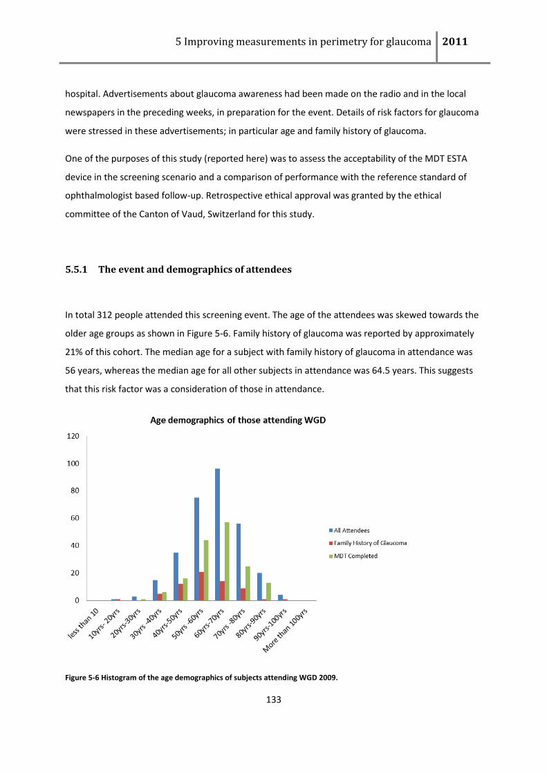
5 Improving measurements in perimetry for glaucoma 2011
133
hospital. Advertisements about glaucoma awareness had been made on the radio and in the local
newspapers in the preceding weeks, in preparation for the event. Details of risk factors for glaucoma
were stressed in these advertisements; in particular age and family history of glaucoma.
One of the purposes of this study (reported here) was to assess the acceptability of the MDT ESTA
device in the screening scenario and a comparison of performance with the reference standard of
ophthalmologist based follow-up. Retrospective ethical approval was granted by the ethical
committee of the Canton of Vaud, Switzerland for this study.
5.5.1 The event and demographics of attendees
In total 312 people attended this screening event. The age of the attendees was skewed towards the
older age groups as shown in Figure 5-6. Family history of glaucoma was reported by approximately
21% of this cohort. The median age for a subject with family history of glaucoma in attendance was
56 years, whereas the median age for all other subjects in attendance was 64.5 years. This suggests
that this risk factor was a consideration of those in attendance.
Figure 5-6 Histogram of the age demographics of subjects attending WGD 2009.
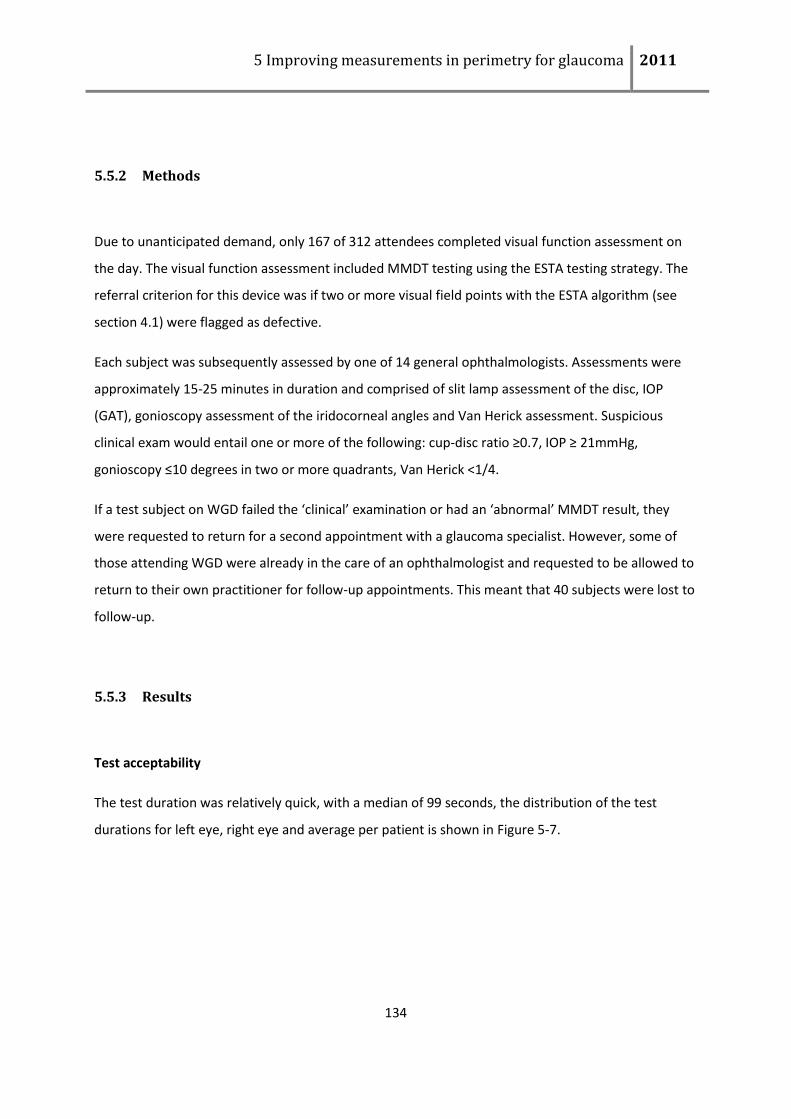
5 Improving measurements in perimetry for glaucoma 2011
134
5.5.2 Methods
Due to unanticipated demand, only 167 of 312 attendees completed visual function assessment on
the day. The visual function assessment included MMDT testing using the ESTA testing strategy. The
referral criterion for this device was if two or more visual field points with the ESTA algorithm (see
section 4.1) were flagged as defective.
Each subject was subsequently assessed by one of 14 general ophthalmologists. Assessments were
approximately 15-25 minutes in duration and comprised of slit lamp assessment of the disc, IOP
(GAT), gonioscopy assessment of the iridocorneal angles and Van Herick assessment. Suspicious
clinical exam would entail one or more of the following: cup-disc ratio ≥0.7, IOP ≥ 21mmHg,
gonioscopy ≤10 degrees in two or more quadrants, Van Herick <1/4.
If a test subject on WGD failed the ‘clinical’ examination or had an ‘abnormal’ MMDT result, they
were requested to return for a second appointment with a glaucoma specialist. However, some of
those attending WGD were already in the care of an ophthalmologist and requested to be allowed to
return to their own practitioner for follow-up appointments. This meant that 40 subjects were lost to
follow-up.
5.5.3 Results
Test acceptability
The test duration was relatively quick, with a median of 99 seconds, the distribution of the test
durations for left eye, right eye and average per patient is shown in Figure 5-7.
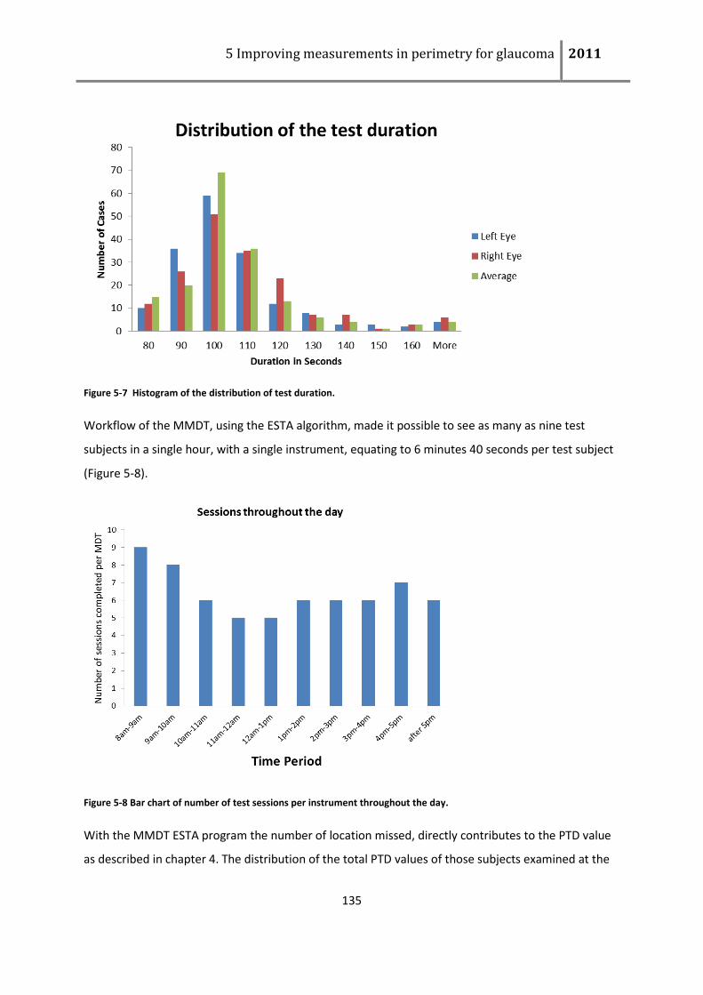
5 Improving measurements in perimetry for glaucoma 2011
135
Figure 5-7 Histogram of the distribution of test duration.
Workflow of the MMDT, using the ESTA algorithm, made it possible to see as many as nine test
subjects in a single hour, with a single instrument, equating to 6 minutes 40 seconds per test subject
(Figure 5-8).
Figure 5-8 Bar chart of number of test sessions per instrument throughout the day.
With the MMDT ESTA program the number of location missed, directly contributes to the PTD value
as described in chapter 4. The distribution of the total PTD values of those subjects examined at the
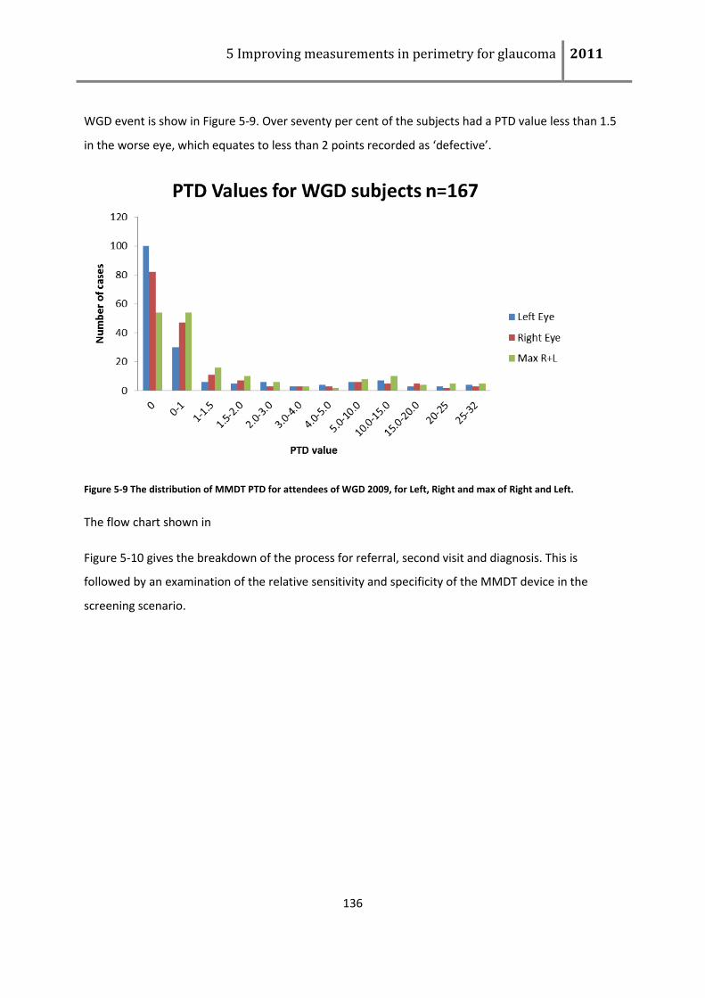
5 Improving measurements in perimetry for glaucoma 2011
136
WGD event is show in Figure 5-9. Over seventy per cent of the subjects had a PTD value less than 1.5
in the worse eye, which equates to less than 2 points recorded as ‘defective’.
Figure 5-9 The distribution of MMDT PTD for attendees of WGD 2009, for Left, Right and max of Right and Left.
The flow chart shown in
Figure 5-10 gives the breakdown of the process for referral, second visit and diagnosis. This is
followed by an examination of the relative sensitivity and specificity of the MMDT device in the
screening scenario.
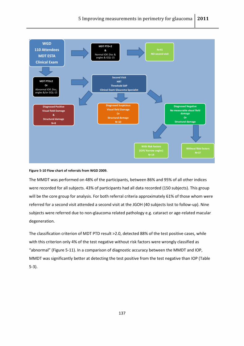
5 Improving measurements in perimetry for glaucoma 2011
137
WGD
110 Attendees
MDT ESTA
Clinical Exam
MDT PTD≥2
Or
Abnormal IOP, Disc, angles &/or GQL-15
Second Visit
HRT
Threshold SAP
Clinical Exam Glaucoma Specialist
Diagnosed Positive
Visual field Damage
&
Structural damage
N=8
Diagnosed Suspicious
Visual field Damage
Or
Structural damage
N=10
Diagnosed Negative
No measurable visual field damage
Or
Structural damage
With Risk Factors
(IOP/ Narrow angles)
N=14
Without Risk factors
N=37
MDT PTD<2
&
Normal IOP, Disc & angles & GQL-15
N=41
NO second visit
Figure 5-10 Flow chart of referrals from WGD 2009.
The MMDT was performed on 48% of the participants, between 86% and 95% of all other indices
were recorded for all subjects. 43% of participants had all data recorded (150 subjects). This group
will be the core group for analysis. For both referral criteria approximately 61% of those whom were
referred for a second visit attended a second visit at the JGOH (40 subjects lost to follow-up). Nine
subjects were referred due to non-glaucoma related pathology e.g. cataract or age-related macular
degeneration.
The classification criterion of MDT PTD result >2.0, detected 88% of the test positive cases, while
with this criterion only 4% of the test negative without risk factors were wrongly classified as
“abnormal” (Figure 5-11). In a comparison of diagnostic accuracy between the MMDT and IOP,
MMDT was significantly better at detecting the test positive from the test negative than IOP (Table
5-3).
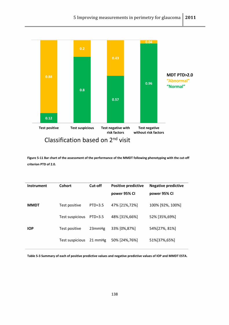
5 Improving measurements in perimetry for glaucoma 2011
138
Figure 5-11 Bar chart of the assessment of the performance of the MMDT following phenotyping with the cut-off
criterion PTD of 2.0.
Table 5-3 Summary of each of positive predictive values and negative predictive values of IOP and MMDT ESTA.
Instrument Cohort Cut-off Positive predictive
power 95% CI
Negative predictive
power 95% CI
MMDT
Test positive PTD=3.5 47% [21%,72%] 100% [92%, 100%]
Test suspicious PTD=3.5 48% [31%,66%] 52% [35%,69%]
IOP Test positive 23mmHg 33% [0%,87%] 54%[27%, 81%]
Test suspicious 21 mmHg 50% [24%,76%] 51%[37%,65%]
5 Improving measurements in perimetry for glaucoma 2011
139
5.5.4 Discussion
The speed of the ESTA MMDT in the screening scenario is clearly demonstrated in this study. In
Figure 5-8 the number of sessions achieved with one ESTA MMDT device is reported. At peak flow,
nine patients were tested on the same instrument in one hour. It follows that at this time point,
other eye occlusion, test explanation and testing both eyes including any required repeated fields
was taking on average 6.5 minutes. With this type of perimetric screening test, visual field
assessment cannot be labelled as “unfeasible”. This is an important observation for MMDT ESTA.
The results from this study illustrate the utility of the ESTA algorithm on the MMDT, in particular the
usefulness of a quick test that appears to produce ‘reliable’ results. In this study, MMDT ESTA
detected close to 90% of the glaucomatous patients (test positive), while only 4% of visually healthy
subject (test negative without risk factors) were recalled. However, it is very important to note, the
small number of participants and the large proportion lost to follow-up restricts the strength of this
study.
Patient acceptability and clinical practicability of perimetric devices are often undervalued when
determining the quality of visual function assessment. In a recent assessment of patient acceptability
the less patient dependent tests were rated with higher patient acceptability e.g. IOP has higher
patient acceptability than functional tests (Gardiner and Demirel, 2008). In the comparison of these
perimetric tests the FDT MATRIX rated higher than the SWAP despite having the longer test duration
(Gardiner and Demirel, 2008). This difference was attributed to ‘increased mental fatigue and
frustration caused by uncertainty about whether they saw the stimulus or not’. If the test is easier to
understand, for example is on a familiar platform like a laptop, and is of a short duration, then it
follows that both the patient and the clinician will be more willing to repeat the exam if there is a
doubtful result. Repeated fields will reduce the number of abnormal results, for example a reduction
of 30% was reported with the FDT1 in the screening scenario (Mansberger et al., 2007).
6 The effect of induced intraocular stray light on perimetric tests
As outlined in the introduction to this thesis perimetry has become a well-established and valuable
tool for the detection and monitoring of sensitivity loss that accompanies various diseases of the
visual pathway, especially glaucoma. While the structure/function debate continues, no consensus
has been reached on why, in some individuals, structural loss is observed at a retinal level before
functional loss is identified with standard automated (contrast) perimetry (SAP) using a white-on-
white stimulus (Quigley et al., 1982, Harwerth et al., 1999, Fraser and Manvikar, 2005). This has
prompted a search for newer perimetric techniques designed to detect functional changes earlier,
however these newer stimuli type may prove more robust to factors that affect the measurement of
retinal function. The seemingly reduced diagnostic sensitivity of perimetry is due, to a large degree,
to inherent variability within the normative data and measurement noise (Artes et al., 2002b). With
age being an important risk factor for glaucoma, it is imperative that other causes of age-related
losses of vision (particularly optical deficits) are accounted for when quantifying neural loss due to
pathology.
There have been many studies demonstrating the effect of cataract on visual field sensitivity, mainly
by comparing visual function before and after cataract extraction and intraocular lens implantation.
In several studies, Standard Automated Perimetry (SAP)(Lam et al., 1991, Hayashi et al., 2001,
Membrey and Fitzke, 2001) and Frequency Doubling Technology (FDT)(Tanna et al., 2004, Membrey
and Fitzke, 2001, Siddiqui et al., 2005) mean deviation was significantly reduced in the presence of
cataract. Although it is recognised that cataract can significantly affect perimetric thresholds, the
degree and nature of lens opacity or cataract was often poorly quantified or characterised in these
studies. In addition, it is not immediately clear which particular aspects of optics confound the
quantification of neural vision loss to the greatest degree. The ageing lens displays changes in general
light absorption (Werner, 1982, Pokorny et al., 1987) forward and backward light scatter (Van den
Berg et al., 2007) and spectral transmission characteristics (Said and Weale, 1959, Ruddock, 1965,
Sample et al., 1988). The relative contribution of each of these to perimetric threshold increase is not
clearly understood.
One result of ageing in general, and cataract formation in particular, is an increase in intraocular
stray light (IOS), arising from increased forward light scatter (de Waard et al., 1992, Van den Berg and
Od, 1995, Van den Berg et al., 2007). Increases in IOS cause a shortening and widening of the point-
spread function of the eye, resulting in reduced contrast sensitivity. Although IOS varies between
6 Improving measurements in perimetry for glaucoma 2011
141
individuals, even in the young healthy eye, largely as a result of differing ocular pigmentation
(Franssen et al., 2007, Van den Berg and Od, 1995), IOS values associated with cataract are greater
(de Wit et al., 2006, Ijspreet et al., 1990). It is reasonable to expect that some perimetric stimuli
might be more susceptible to the influence of additional IOS than others (as some are being
modulated in contrast while others are being modulated along a spatial scale). It follows that of the
various forms of commercially available perimeters (which often employ different stimulus types
with different configurations) some may be affected more than others with additional IOS.
Several studies have used white diffusing filters during perimetry to simulate the effects of cataract
(de Wit et al., 2006, Wood et al., 1987, Membrey et al., 1999, Budenz et al., 1993). These studies
have shown a general depression of the hill of vision with SAP (on both the Humphrey Field Analyzer
and the Octopus perimeter) and FDT perimetry; there were significant reductions in sensitivity after
the introduction in front of the eye of diffusing filters consisting of photographic filter foils (Membrey
et al., 1999), 500nm latex beads (Wood et al., 1987) or ground glass (Budenz et al., 1993). The results
found with these cataract simulations were consistent with those reported in patient cases of pre-
and post-operative cataract removal, although the degree of simulated cataract was not quantified in
a way that could be correlated with physiological or pathological states of the eye’s optical quality.
Membrey et al (1998) carried out a study to investigate the effects of simulated cataract (using one
white diffusing filter) on the FDT (FDT1, 24-2), SAP (HFA II, Full Threshold) and a prototype Motion
Discrimination Test (MMDT) (using single line presentation) and comparisons were made between
these three instruments using standardised values for the thresholds. They concluded that the
MMDT stimulus was more resilient to this form of simulated cataract compared to the stimuli used in
SAP and FDT. Significant modifications have been made to the test strategies, formats and stimuli
used in these clinical devices since this study was conducted and the relationship between the
properties of the diffusing filter and the various forms of lens opacity is not well defined.
Diffusing filters used for cataract simulation have traditionally been characterised either nominally or
by their optical density. However, a recent study by de Wit et al has considered the use of diffusing
filters as a simulation of cataract (de Wit et al., 2006) by comparing the light scattering properties of
the filters with those of cataract. Anderson et al, recently investigated the effects of intraocular stray
light, induced by white opacity filters (WOFs; LEE Filters, Andover, UK) of different grades on various
forms of perimetry (SAP, FDT1, short-wavelength automated perimetry (SWAP) and peripheral
grating resolution perimetry (GRP))(Anderson et al., 2009). The WOFs contain light-scattering
6 Improving measurements in perimetry for glaucoma 2011
142
particles within the matrix of the polymer rather than etchings on the surface, resulting in wide angle
scatter similar to that caused by cataract (Anderson et al., 2009, de Wit et al., 2006, Franssen et al.,
2007). A particular strength of the study by Anderson and colleagues (Anderson et al., 2009) was that
the magnitude of intraocular stray light induced by each filter was quantified using the Oculus C-
Quant cataract quantifier (Oculus, Wetzlar, Germany) as described by Franssen and colleagues
(Franssen et al., 2006).
The aim of this study is to examine the effect of IOS, using similar methodology to Anderson and
colleagues (Anderson et al., 2009) on threshold measurements for stimuli employed in four
perimeters: namely HFA SAP SITA, FDT MATRIX ZEST, MDT WEBS and HEP FDF ASTA-Std.
The work reported in this chapter has formed a paper published by Investigative Ophthalmology and
Visual Science ((Bergin et al., 2011); See ‘List of supporting publications’). The joint authors of this
work are Ciara Bergin [CB], Tony Redmond [TR], Neil Nathwani [NN], Gay Verdon-Roe [GVR], David
Crabb [DC], Roger Anderson [RA] and David Garway-Heath [DGH]. The experiments were conducted
by CB, TR and NN. The experiment was conceived jointly by all the authors. CB performed all the
data analysis and wrote the manuscript with contributions from all the authors and the work was
supervised by DC and DGH. The results in this chapter have also in part been presented as a poster
presentation at the Association for Research in Vision and Ophthalmology Meeting, Fort Lauderdale,
Florida, USA in May 2009 ((Verdon-Roe et al., 2009); See ‘List of supporting publications’).
6.1 Method to detect difference in measurements with additional stray light
Six healthy, psychophysically experienced volunteers (aged 21-29 [mean 26] years) participated in
this study. None had a history of ocular pathology or systemic disease that may affect visual
performance and none had previous ocular surgery. Inclusion criteria included optic disc rim area
classified as “within normal limits” by Moorfields Regression Analysis of the Heidelberg Retina
Tomograph (HRT II; Heidelberg Engineering, Heidelberg, Germany) and intraocular pressure
<21mmHg. The right eye was tested for all subjects and each wore appropriate near correction,
refractive error ranged from 0 to -4.25 [mean -2.10] dioptres sphere. Subjects had negligible
astigmatism (≤0.50 dioptres cylinder). Best-corrected visual acuity for each observer was 20/17 (6/5)
or better. All subjects were reliable (false positives <20%, false negatives <33% and fixation losses
6 Improving measurements in perimetry for glaucoma 2011
143
<33%) in two initial practice sessions on each perimeter. The study had local ethical approval from
City University, London with recruitment and experimentation adhering to the tenets of the
Declaration of Helsinki.
6.1.1 Perimetric Stimuli
Four types of perimetry were employed namely HFA II; SITA-Standard 24-2 program, FDT Matrix;
24-2 ZEST program, HEP; 24-2 ASTA, MMDT; 32 WEBS. As mentioned previously, each perimeter has
a different stimulus, detection task and thus scale on which threshold is measured. SAP is measured
on an inverse log scale of Michelson contrast, the dynamic range of the instrument is 0dB to 40dB
(which in terms of contrast >99% contrast to <1% contrast). FDT also has a contrast modulated
stimulus, Michelson contrast varies between 100% and 1%, and thresholds are measured on a log
scale ranging from 0dB to 38dB. FDF on the Heidelberg Edge Perimeter (HEP) is also a contrast
modulated stimulus, Michelson contrast varies between 100% and 1%, and is measured on a log
scale ranging from 0dB to 22dB. Within the software there is a default scale has been transformed to
match the dynamic range to that of the HFA clinical instrument. For this study we used the non-
transformed version of threshold measures from the HEP. Finally, the stimulus of the MMDT is
modulated in magnitude of displacement; displacements vary between 2min of arc and 40 min of
arc.
6.1.2 White Opacity Filters (WOF)
Five white resin opacity-containing filters were used (Fog 1 to 5). These WOFs had mean light
transmittance spectra ranging from 0.86 (Fog 1) to 0.42 (Fog 5) as measured against an achromatic
CRT screen (luminance: 10cd/m2; x = 0.218, y = 0.328) For ease of use, these filters were cut and
edged into spectacle frames with large aperture lens. Blenderm tape over a blank lens was used to
occlude the non-test eye in order to eliminate the detection of form or movement.
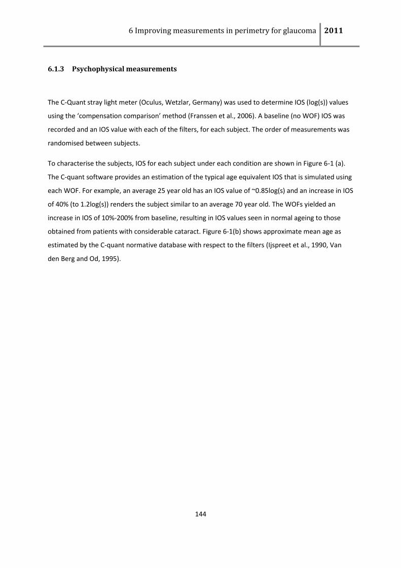
6 Improving measurements in perimetry for glaucoma 2011
144
6.1.3 Psychophysical measurements
The C-Quant stray light meter (Oculus, Wetzlar, Germany) was used to determine IOS (log(s)) values
using the ‘compensation comparison’ method (Franssen et al., 2006). A baseline (no WOF) IOS was
recorded and an IOS value with each of the filters, for each subject. The order of measurements was
randomised between subjects.
To characterise the subjects, IOS for each subject under each condition are shown in Figure 6-1 (a).
The C-quant software provides an estimation of the typical age equivalent IOS that is simulated using
each WOF. For example, an average 25 year old has an IOS value of ~0.85log(s) and an increase in IOS
of 40% (to 1.2log(s)) renders the subject similar to an average 70 year old. The WOFs yielded an
increase in IOS of 10%-200% from baseline, resulting in IOS values seen in normal ageing to those
obtained from patients with considerable cataract. Figure 6-1(b) shows approximate mean age as
estimated by the C-quant normative database with respect to the filters (Ijspreet et al., 1990, Van
den Berg and Od, 1995).
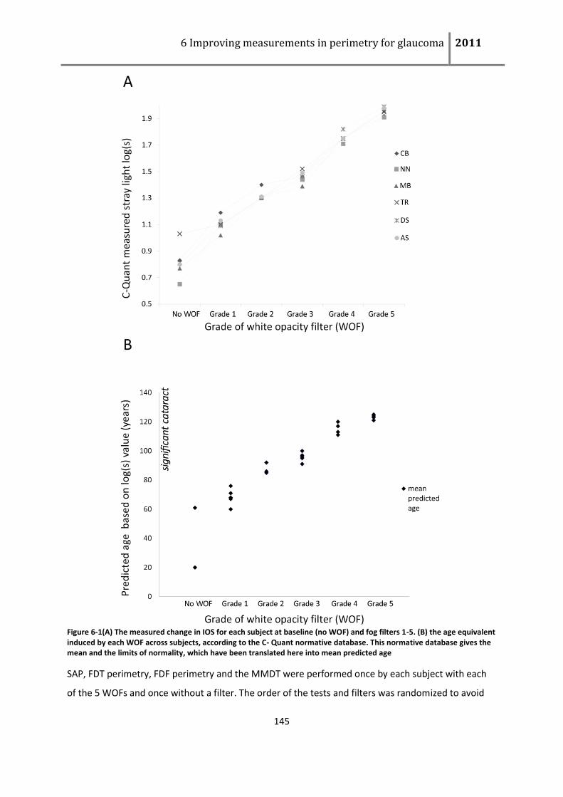
6 Improving measurements in perimetry for glaucoma 2011
145
Figure 6-1(A) The measured change in IOS for each subject at baseline (no WOF) and fog filters 1-5. (B) the age equivalent induced by each WOF across subjects, according to the C- Quant normative database. This normative database gives the mean and the limits of normality, which have been translated here into mean predicted age
SAP, FDT perimetry, FDF perimetry and the MMDT were performed once by each subject with each
of the 5 WOFs and once without a filter. The order of the tests and filters was randomized to avoid
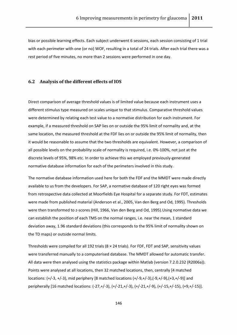
6 Improving measurements in perimetry for glaucoma 2011
146
bias or possible learning effects. Each subject underwent 6 sessions, each session consisting of 1 trial
with each perimeter with one (or no) WOF, resulting in a total of 24 trials. After each trial there was a
rest period of five minutes, no more than 2 sessions were performed in one day.
6.2 Analysis of the different effects of IOS
Direct comparison of average threshold values is of limited value because each instrument uses a
different stimulus type measured on scales unique to that stimulus. Comparative threshold values
were determined by relating each test value to a normative distribution for each instrument. For
example, if a measured threshold on SAP lies on or outside the 95% limit of normality and, at the
same location, the measured threshold at the FDF lies on or outside the 95% limit of normality, then
it would be reasonable to assume that the two thresholds are equivalent. However, a comparison of
all possible levels on the probability scale of normality is required, i.e. 0%-100%, not just at the
discrete levels of 95%, 98% etc. In order to achieve this we employed previously-generated
normative database information for each of the perimeters involved in this study.
The normative database information used here for both the FDF and the MMDT were made directly
available to us from the developers. For SAP, a normative database of 120 right eyes was formed
from retrospective data collected at Moorfields Eye Hospital for a separate study. For FDT, estimates
were made from published material (Anderson et al., 2005, Van den Berg and Od, 1995). Thresholds
were then transformed to z-scores (Hill, 1966, Van den Berg and Od, 1995).Using normative data we
can establish the position of each TMS on the normal ranges, i.e. near the mean, 1 standard
deviation away, 1.96 standard deviations (this corresponds to the 95% limit of normality shown on
the TD maps) or outside normal limits.
Thresholds were compiled for all 192 trials (8 × 24 trials). For FDF, FDT and SAP, sensitivity values
were transferred manually to a computerised database. The MMDT allowed for automatic transfer.
All data were then analysed using the statistics package within Matlab (version 7.2.0.232 (R2006a)).
Points were analysed at all locations, then 32 matched locations, then, centrally [4 matched
locations: (+/-3, +/-3), mid periphery [8 matched locations (+/-9,+/-3),(-9,+/-9),(+3,+/-9)] and
peripherally [16 matched locations: (-27,+/-3), (+/-21,+/-3), (+/-21,+/-9), (+/-15,+/-15), (+9,+/-15)].
6 Improving measurements in perimetry for glaucoma 2011
147
Since the results of this study were consistent throughout only those results from “all locations” are
reported below
6.3 Degree of the effect of IOS
Examining the change in Mean Deviation (MD), from baseline to WOF5 is clinically significant in SAP
FDT and FDF (SAP=-4.4dB; FDT=-6.5dB; MDT=+0.7Min of Arc and FDF=10.1dB). Since each instrument
measures along a different scale, we cannot compare one instrument with another; however we can
examine how each instrument behaves with increases in IOS. A two-way ANOVA with subjects acting
as blocks in the experiment and the main factor being each grade of WOF indicated that MD as
measured with FDT, SAP and FDF worsens across the different WOF (P<0.0001). Conversely, there
was no evidence of a difference in MD values for MMDT across the different WOFs (P=0.18).
Threshold Mean Sensitivity (TMS) is the average measured sensitivity; we examined the relationship
between TMS and grade of WOF used. We found that with WOF greater than grade 4, SAP (p<.001),
FDT (p=0.003) and FDF (p<0.001) were highly significantly affected and MMDT TMS values did not
have a significant association with the density of FOG filter used (p=0.73) (ANOVA).
All subjects had different stray light values for each of the WOF filters used. To reduce the spread of
the data points, TMS values were plotted against the respective C-Quant log(s) values; this is
represented in Figure 6-2, here the shaded area represents the approximate normative range for
each instrument. Using linear regression, the dB (or minutes of arc for MMDT) loss per log(s) for each
perimeter is estimated; the FDF, SAP and FDT are all significantly associated (p<.001) by IOS; MMDT
does not have significant slope (p=.34). The estimated slopes were: SAP=-1.6dB/log(s), FDT=-
1.7dB/log(s), FDF=-3.1dB/log(s) and MMDT=-0.1minutes of arc/log(s)).
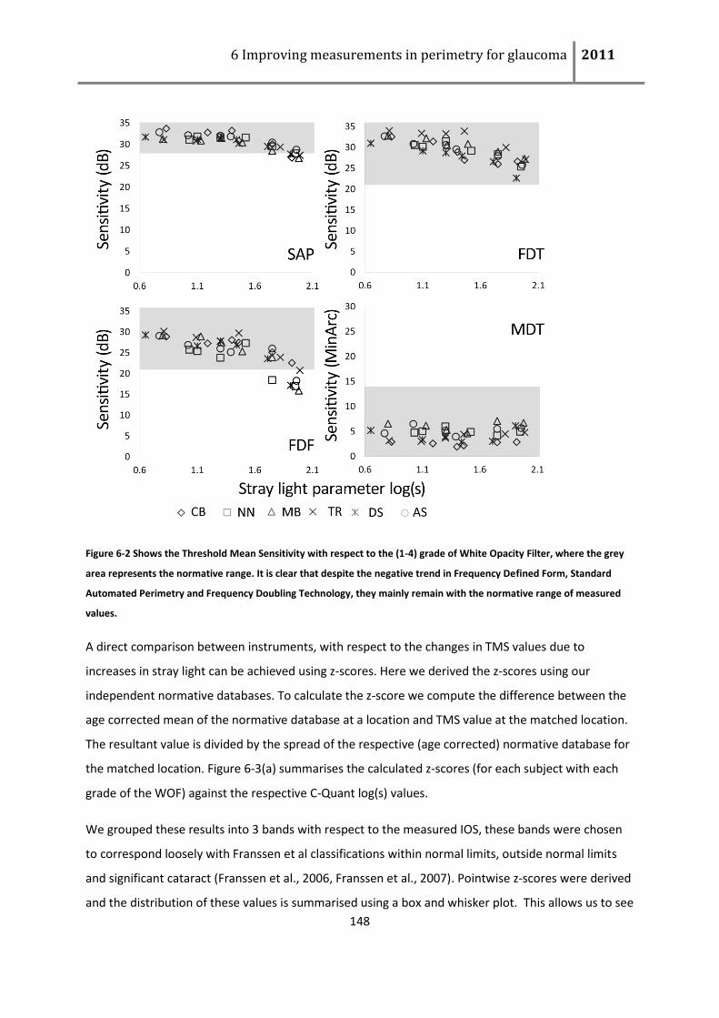
6 Improving measurements in perimetry for glaucoma 2011
148
Figure 6-2 Shows the Threshold Mean Sensitivity with respect to the (1-4) grade of White Opacity Filter, where the grey
area represents the normative range. It is clear that despite the negative trend in Frequency Defined Form, Standard
Automated Perimetry and Frequency Doubling Technology, they mainly remain with the normative range of measured
values.
A direct comparison between instruments, with respect to the changes in TMS values due to
increases in stray light can be achieved using z-scores. Here we derived the z-scores using our
independent normative databases. To calculate the z-score we compute the difference between the
age corrected mean of the normative database at a location and TMS value at the matched location.
The resultant value is divided by the spread of the respective (age corrected) normative database for
the matched location. Figure 6-3(a) summarises the calculated z-scores (for each subject with each
grade of the WOF) against the respective C-Quant log(s) values.
We grouped these results into 3 bands with respect to the measured IOS, these bands were chosen
to correspond loosely with Franssen et al classifications within normal limits, outside normal limits
and significant cataract (Franssen et al., 2006, Franssen et al., 2007). Pointwise z-scores were derived
and the distribution of these values is summarised using a box and whisker plot. This allows us to see
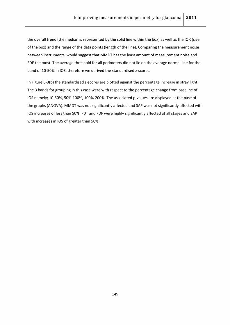
6 Improving measurements in perimetry for glaucoma 2011
149
the overall trend (the median is represented by the solid line within the box) as well as the IQR (size
of the box) and the range of the data points (length of the line). Comparing the measurement noise
between instruments, would suggest that MMDT has the least amount of measurement noise and
FDF the most. The average threshold for all perimeters did not lie on the average normal line for the
band of 10-50% in IOS, therefore we derived the standardised z-scores.
In Figure 6-3(b) the standardised z-scores are plotted against the percentage increase in stray light.
The 3 bands for grouping in this case were with respect to the percentage change from baseline of
IOS namely; 10-50%, 50%-100%, 100%-200%. The associated p-values are displayed at the base of
the graphs (ANOVA). MMDT was not significantly affected and SAP was not significantly affected with
IOS increases of less than 50%, FDT and FDF were highly significantly affected at all stages and SAP
with increases in IOS of greater than 50%.
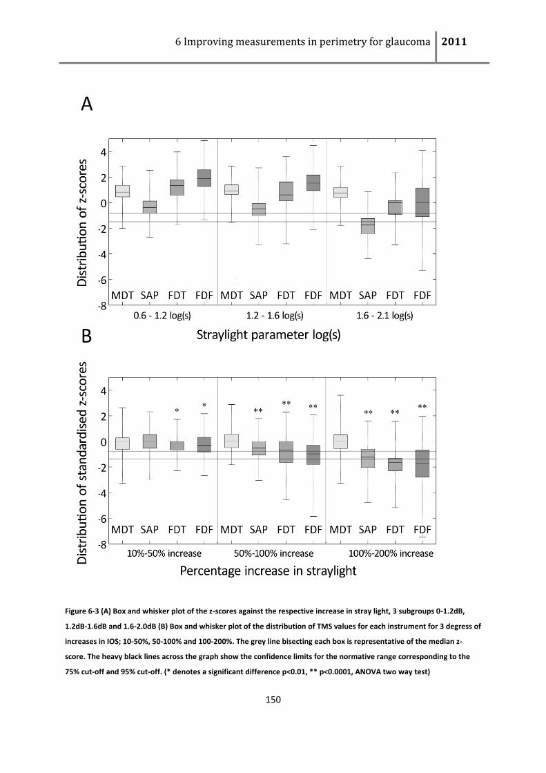
6 Improving measurements in perimetry for glaucoma 2011
150
Figure 6-3 (A) Box and whisker plot of the z-scores against the respective increase in stray light, 3 subgroups 0-1.2dB,
1.2dB-1.6dB and 1.6-2.0dB (B) Box and whisker plot of the distribution of TMS values for each instrument for 3 degress of
increases in IOS; 10-50%, 50-100% and 100-200%. The grey line bisecting each box is representative of the median z-
score. The heavy black lines across the graph show the confidence limits for the normative range corresponding to the
75% cut-off and 95% cut-off. (* denotes a significant difference p<0.01, ** p<0.0001, ANOVA two way test)
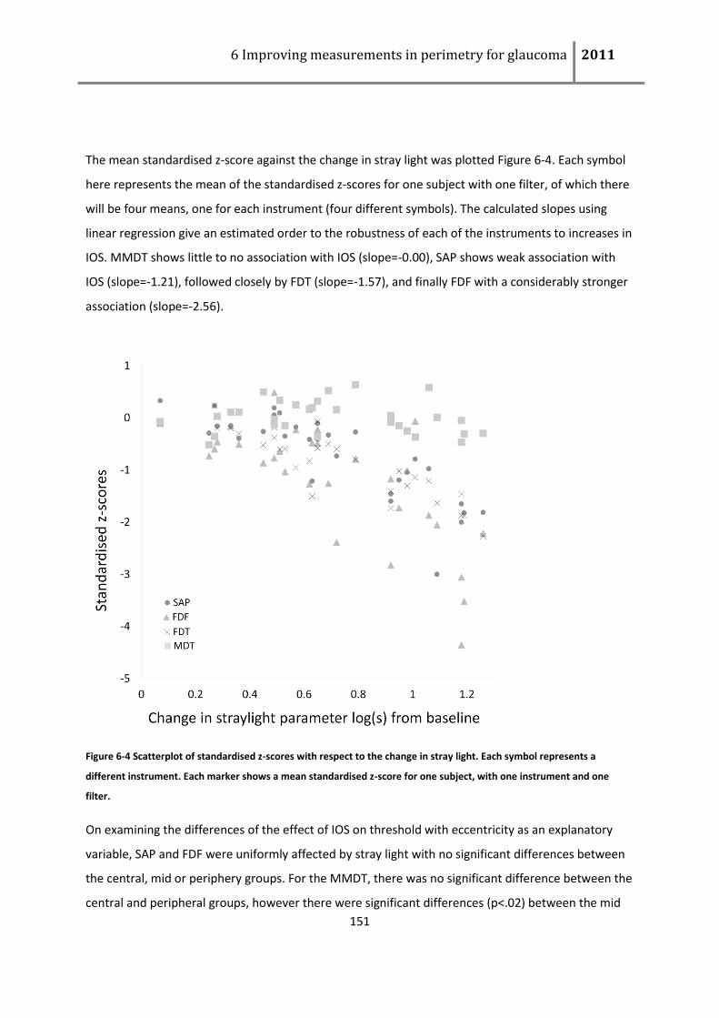
6 Improving measurements in perimetry for glaucoma 2011
151
The mean standardised z-score against the change in stray light was plotted Figure 6-4. Each symbol
here represents the mean of the standardised z-scores for one subject with one filter, of which there
will be four means, one for each instrument (four different symbols). The calculated slopes using
linear regression give an estimated order to the robustness of each of the instruments to increases in
IOS. MMDT shows little to no association with IOS (slope=-0.00), SAP shows weak association with
IOS (slope=-1.21), followed closely by FDT (slope=-1.57), and finally FDF with a considerably stronger
association (slope=-2.56).
Figure 6-4 Scatterplot of standardised z-scores with respect to the change in stray light. Each symbol represents a
different instrument. Each marker shows a mean standardised z-score for one subject, with one instrument and one
filter.
On examining the differences of the effect of IOS on threshold with eccentricity as an explanatory
variable, SAP and FDF were uniformly affected by stray light with no significant differences between
the central, mid or periphery groups. For the MMDT, there was no significant difference between the
central and peripheral groups, however there were significant differences (p<.02) between the mid
6 Improving measurements in perimetry for glaucoma 2011
152
and central and the mid and peripheral groups. For FDT mildly significant differences (p<.05) were
found between the central and mid-range groups. This may have be effect by the reduced Michelson
contrast and change in length of line stimuli (energy) see discussion.
6.4 Discussion
Perimetry has two purposes, for monitoring disease and for case-detection. For both roles, it is
important that the test result is not confounded by eye conditions other than the ‘target’ condition
(in this case glaucoma). For monitoring, progressive cataract in glaucomatous patients or suspects
may result in a change in thresholds that may mimic progressive glaucoma. For case-detection,
considering IOP level is a risk factor for glaucoma, but does not define the disease (Weinreb, 2007),
and sophisticated imaging devices are expensive for primary care settings, therefore many clinicians
rely on perimetric tests for diagnosis. It is unsurprising then that often false positive results may arise
from cataract. Thus, it would be advantageous to have a perimetric test that is robust to the effects
of cataract.
An analysis developed to compensate for the effects of loss of optical quality is the addition of
Pattern Deviation (PD) maps (as in STATPAC for the Humphrey Field Analyser). PD measures partly
account for diffuse (typically optical) loss by subtracting from the total deviation plot (deviation from
the sensitivity of age-matched normals), the value corresponding to the 85th centile of the TD
measures thus amplifying focal loss in the pattern deviation plot. However, this diffuse loss is not
individualised with respect to expected reduction in sensitivity due to loss of optical quality. For this
reason when diffuse loss is accounted for with summary measures such as PSD in the HFA, diffuse
glaucomatous loss is hidden. Thus, although pattern deviation plots are useful in that they help
identify sites of focal loss, they remain of limited value.
In this study we have created IOS environments ranging from those associated with normal ageing to
those encountered with significant cataract. This has allowed us to demonstrate the effect of various
levels of intraocular stray light on perimetric thresholds and give measure of the robustness of each
instrument to such ocular imperfections. Throughout the range of IOS levels, the MMDT stimulus
remained relatively robust while each of the other perimeters suffered greater loss in sensitivity with
markedly increased IOS.
6 Improving measurements in perimetry for glaucoma 2011
153
Using these WOFs we have attempted to demonstrate not only the effects on modern perimetry of
the additional IOS equivalent to those due to ageing but also with significant cataract. Real cataracts
have typically been graded in four different categories depending on location, colour, density and
shape of the opacity within the lens (Chylack et al, 1993). The WOFs used in this study are uniform
density filters and, as such, are simulations of only one form of cataract.
The spatial characteristics of the test stimuli may account for the notable difference in robustness to
the effects of IOS between the tests. Stimuli employed in SAP, FDT and FDF are contrast-modulated,
whereas the MMDT stimulus remains at constant contrast and the magnitude of displacement is
modulated. So while the MMDT suffers an approximate 10-20% decrease in Michelson contrast at
displacements at reference threshold, alternative contrast modulated methods may suffer 70-80%
decrease in contrast at respective reference thresholds. This result is therefore not surprising given
that contrast suffers at the hands of optical imperfections arising from conditions such as cataract.
Further to this we measured luminance for the MMDT stimuli with the densest of these WOF (FOG 5)
we calculated resultant energy where energy is a composite of area and change in luminance
between the stimulus and the background as described by Verdon-Roe et al. Using the relationship
between energy and MMDT threshold, we calculated the expected threshold with and without FOG 5
. We found that for stimuli of length greater than about 40 min of arc the estimated drop in
threshold according to this relationship should be less than 5 mins of arc, which is less than 2
standard deviations of the normative database, and so may not reach significance.
Anderson et al found a similar result for robustness with their peripheral grating resolution perimetry
(GRP) test; notably it is also a less contrast dependent test (Anderson et al., 1995, Anderson et al.,
2002, Anderson, 1996).
The effect of IOS on SAP thresholds is similar but less marked in this study compared to that of
Anderson et al (4.9dB/log(s) versus 3.5dB/log(s), respectively (Anderson et al., 2009). The difference
may be accounted for by the greater number of test locations in the present (52) as opposed to only
4 central test locations used in the analysis of Anderson et al (Anderson et al., 2009). On examining
the differences between central and peripheral locations with SAP and FDT from this study we found
that peripheral locations were weakly significantly more affected with IOS (p<.05). Also we compared
FDT1 from Anderson et al with FDT Matrix result from this study. However, we are conscious that the
stimulus size and testing procedures, screen resolution and appearance of each of these instruments
differ somewhat. The size of the effect in terms of z-scores is slightly greater (1.3/log(s) with FDT1
6 Improving measurements in perimetry for glaucoma 2011
154
versus 1.6/log(S) with FDT Matrix) and this may be due to the additional peripheral locations and also
the reduced stimulus size of the Matrix FDT (5 degree patch versus 10 degree patch of FDT1).
There is a need for further clarification of the role of IOS log(s) in baseline values in perimetry. Here,
we demonstrate measurable effects of increases in IOS, equivalent to those related to age, on SAP,
FDT and FDF (Figure 6-3 and Figure 6-4. The correlation of stray light with spread of normative values
may lead to tightening of normative ranges, or an improvement to standard normative databases as
suggested by Anderson et al(Anderson et al., 2009). This may lead to a methodology to correct for
the current issue with diffuse glaucomatous loss and clinical contrast modulated standard perimetric
measures. Tighter normal ranges would facilitate the identification of subtle sensitivity loss and
provide greater confidence for diagnostic decisions. Therefore further exploration of the influence of
individual IOS measures on the normative databases is required.
The main conclusion to be drawn from the study reported in this chapter has important ramifications
for the practical use of perimetric instruments. There was little difference in the performance of FDT
and SAP with respect to increases in IOS, both were significantly affected. FDF appears to be quite
sensitive to increases in IOS in comparison to SAP and FDT. There was little to no appreciable effect
of IOS on MMDT thresholds.
7 Conclusions
Glaucoma is the leading cause of preventable blindness worldwide. Automated perimetry currently
offers the best measure of functional impairment from the condition. However, the high level of
noise in automated perimetry erodes the value of these measurements. Reduction in this noise,
whether it comes in the form of better performing testing algorithms, or greater resilience of
perimetric stimuli to forms of optical blur or media opacity, is a welcome advance.
7.1 Summary of thesis
In chapter 2, the effect of eccentricity and threshold on the MMDT stimulus type was explored in
patients and visually healthy control subjects using a FOS analysis; this had not been done previously.
The primary outcome of this chapter was a sample of carefully collected FOS data collected in
patients and controls that could be used to develop reference standards and models for testing the
perimetric algorithms developed in subsequent chapters.
In chapter 3, a review of the types of clinical threshold search methods currently available was made.
A best parametric type algorithm and best non-parametric type algorithm (WEBS and NEST) were
modified and applied to the MMDT stimulus. The performance of these two algorithms was
compared against standard staircases that were initially implemented in the MMDT. Analyses of the
patient data approach and ORS approach were reported. The newer methods showed significant
improvements over the staircases. The ORS approach in particular showed that WEBS and ZEST were
less affected by start point and step size than staircases.
In chapter 4, a novel suprathreshold testing algorithm, ESTA, was developed. As in chapter 3, the
performance of this algorithm was then compared with alternative suprathreshold algorithms using
only the patient data approach. In the patient data approach the significant reduction in test
duration in comparison to multisampling suprathreshold perimetry was shown, while agreement
with the reference standard remained at a similar level for all suprathreshold methods. The
investigation into the diagnostic performance of the algorithm was limited by the sample size. Still,
7 Improving measurements in perimetry for glaucoma 2011
156
the ESTA algorithm provides a novel promising rapid perimetric strategy for glaucoma detection and
it has been patented (see ‘List of supporting publications’).
In chapter 5, studies using the test algorithms developed in the work described in this thesis (MMDT
WEBS and MMDT ESTA) were reported. In the main, these interim results suggest there is no
significant difference in the diagnostic accuracy of either MMDT WEBS or MMDT ESTA with any of
the compared devices. For example, the interim analysis suggests that the relative diagnostic
precision of the screening strategies for SAP (64-point screening), FDT1 (C20), MMDT (ESTA) in the
clinic-based population of early glaucomatous patients are equivalent. FDT1 (17 test points) and MDT
(32 test points) are quicker to perform than the SAP screening strategy. A further study reported in
this chapter indicated how the MMDT, running the ESTA algorithm in a ‘screening event, gives
evidence of the utility of this technique, suggesting that the device is truly portable and quick,
without losing accuracy for detection.
Chapter 6 reported a study examining the effect of intraocular stray light (IOS) on threshold
measurements made by four types of perimetry: Standard Automated Perimetry (SAP), Frequency
Doubling Technology Perimetry (FDT), the Frequency Defined Form (FDF) and the Moorfields Motion
Displacement Test (MMDT). Average response to SAP, FDT and FDF were highly affected by
moderate to large increases in IOS while MDT remained largely unaffected over the same range of
stray light levels. This work, being the first of its kind, indicates that MMDT has greater resilience to
simulated effects of media opacity compared with other clinically used devices. The practical
ramifications of this finding suggest that the MMDT stimulus could be preferred over other devices
when case finding glaucoma in the elderly population where media degradation in eyes will abound.
In summary, the key contributions, in order of importance, of the work described in this thesis to the
field of perimetry in glaucoma are:
Production of the novel suprathreshold testing method ESTA, which has been implemented
on the MMDT device. This work has title of a US and UK patent (see ‘List of supporting
publications’).
7 Improving measurements in perimetry for glaucoma 2011
157
Demonstration of the resilience of the MMDT to optical media opacity when compared to
other perimetric instruments.
Production of a clinical threshold search method (test algorithm) which is less variant with
respect to step size and starting point as compared to current used methods on the MMDT.
Providing interim results on the performance of the MMDT against other perimetric devices
in an instrument comparison study.
Providing frequency of seeing data in glaucomatous patients with the multi-locational
MMDT.
7.2 Future work
Several projects originating from outcomes of this thesis have already begun:
Examine additional perimetric devices to determine the effect of intraocular stray light.
Examining the resilience of the MMDT in comparison to alternative perimetric devices to
media opacity in pre and post cataract extraction patients.
Matching the dynamic ranges of SAP and MMDT using FOS data collection.
A search for a clinically acceptable FOS data collection algorithm to identify and eliminate
highly variable subjects/areas of loss from threshold data acquisition.
Development of a clinical threshold test which is a hybrid of FOS data collection and
suprathreshold assessment.
In conclusion, the MMDT appears to have some advantages over alternative perimetric methods,
such as robustness to increases in IOS (as demonstrated in chapter 6). Combined with the short test
duration delivered with the suprathreshold test ESTA (described in chapter 4), the test appears to
perform well in the screening environment (section 5.5). When compared to alternative perimetric
instruments, MMDT ESTA does not perform significantly differently in terms of diagnostic accuracy

7 Improving measurements in perimetry for glaucoma 2011
158
(section 5.1-5.4). Therefore, these results would suggest that the MMDT ESTA instrument would be
clinically useful as a case finding test for the community optometrist. Several studies are currently
investigating this.
Robustness to moderate levels of optical blur has been reported with the MMDT (-6.00DS: +4.00DS
Moosavi 2011; In submission), which removes the need for optical correction in the majority of
cases. Furthermore, the MMDT has reportedly low learning effects (Moosavi 2011; In submission)
which is likely to be related to the familiar hardware used, which will should reduce the need for
repeat testing and reduce the number of false referrals. Robustness to learning and optical blur will
also have significant implications for speed in the screening environment.
Screen characteristics play a large role in the development of the threshold monitoring version of the
MMDT. The MDT stimulus is set at 85% Michelson contrast however, with LCD screens and with
laptop LCD screens in particular, uniform contrast is difficult to maintain throughout the screen.
Currently each piece of hardware has to be calibrated manually. Moreover due to the restrictions of
pixel pitch with current screen technology, the threshold version of the MMDT has proved more
difficult to develop. However with the speed of technological advancement and introduction of
organic screens in particular, this restriction should soon be insignificant. The selection of
measurement scale that is calibrated to functional loss, such that uniformity between degree of
functional loss and MMDT measures is the next point of research (see 1.4.3). Since the relative step
size on the end of the measurement scale corresponding to functional loss would be increased (e.g.
the log scale of SAP does this in part) this should increase relative precision with threshold
estimation.
The construction of an ORS similar to that reported in this thesis which is robust enough for spatial
simulation would be useful but very difficult to achieve. Intense data collection at a large number of
locations throughout the field in a larger cohort of subjects (visually healthy and glaucomatous)
would be required. The incorporation of fatigue and learning would also be required to form an ORS
robust enough to simulated ESTA like procedures, in search procedures which are as short as ESTA
the learning effect will have a highly variable impact, which will be difficult to simulate correctly.
The development of ‘better’ threshold algorithms has long been attempted. There is no easy answer
to whether further investigation will yield significant results, and the low signal to noise ratio
7 Improving measurements in perimetry for glaucoma 2011
159
associated with perimetric testing suggest that improvements will always be difficult to make. The
construction of the WEBS procedure reported in this thesis outperformed the current methods used
for threshold assessment in the MMDT, however the implementation of individualised tests, where
either previous perimetric tests result are utilised in retesting (e.g. REMU (Turpin et al., 2007)) or
structural measures are used to inform and focus perimetric testing (Turpin et al, 2009) may provide
more reliable perimetric results. What was apparent from this work is that the slope of the frequency
of seeing curve has a significant impact on precision, notably subjects with shallow slopes or low
response confidence will always provide highly variable results. These subjects would likely perform
better with suprathreshold testing, where the size of the defect is monitored rather than the depth.
A method to identify these subjects early and eliminate from further threshold testing may prove
useful.
Baseline FOS data on all subjects could provide a method to identify these subjects. Clinical FOS data
collection at a large number locations would be unfeasible, however a suprathreshold threshold
method which migrated into intense sampling at one location in each disc quadrant (as defined by a
given map e.g. Garway-Heath 2000), may provide the relevant information for structure/function
assessment, broad functional information on size of defects and the necessary information on
reliability. This information on reliability of each of the quadrants could then be used to estimate
interpretation error (King-Smith 1994), the larger the interpretation error the more noise in
measures and the more difficult it will be to detect change (signal). Pre-set limits on signal to noise
ratios could then be used to determine whether it would be useful to any threshold information in
this quadrant. The additional benefit of this method is that the baseline could be repeated at any
stage and the FOS curves compared allowing disease progression to monitored with respect to
changes in threshold and changes in slope.

8 List of supporting publications
Peer reviewed papers
C. Bergin, D. F. Garway-Heath, D. P. Crabb. (2008)
Evaluating the effect of the new alignment algorithm for longitudinal series of Heidelberg retina
tomography images Acta Ophthalmologica 86 (2), 207–214
C Bergin, T Redmond, N Nathwani, GM Verdon-Roe, DP Crabb, RS Anderson DF Garway-Heath (2011)
The effect of induced intraocular stray light on perimetric tests Invest. Ophthalmol. Vis. Sci. Vol 52
No 6 3676-3682
Patents:
C.Bergin, DF Garway-Heath, DP Crabb, GM Verdon-Roe, M Westcott.
A Supra-Threshold Test for Use in Detecting Sensitivity Loss Across the Field of Vision [UK priority
application 1007697.4 and US priority application 61/332023], Applicant: UCLB,
Meeting abstracts
C. Bergin, R. Moosavi, D. P. Crabb, G. M. Verdon-Roe, M. Westcott, A. C. Viswanathan1, F. W. Fitzke,
D. F. Garway-Heath.
Developing and Evaluating Threshold Algorithms for the Moorfields Motion Displacement Test (MDT)
Invest. Ophthalmol. Vis. Sci. 2008 49: E-Abstract 1108
C. Bergin, R. Moosavi, G.M. Verdon-Roe, D.P. Crabb, M.C. Westcott, A.C. Viswanathan, F.W. Fitzke,
D.F. Garway-Heath. (2008)
How do different test strategies for estimating perimetry thresholds behave when the dynamic range
of measurement varies? 18th Imaging and Perimetric Society Symposium. Nara, Japan, May 2008
C. Bergin, G.M. Verdon-Roe, D. P. Crabb, M. Westcott, A. C. Viswanathan, F. W. Fitzke, and D. F.
Garway-Heath.
8 Improving measurements in perimetry for glaucoma 2011
161
New Advances in Moorfields Motion Displacement Perimetry. UK&Eire Glaucoma Society Meeting,
Dublin, December 2008
C. Bergin, D. P. Crabb, R. Moosavi, G.M. Verdon-Roe, M.C. Westcott, D.F. Garway-Heath. (2009)
Enhanced Supra-Threshold Testing Algorithm: A New Tool for Rapid Detection of Visual Field Loss
Invest. Ophthalmol. Vis. Sci. 2009 : E-Abstract 6196
G. M. Verdon-Roe, C. Bergin, T. Redmond, N. Nathwani, D. P. Crabb, R.S. Anderson and D. F. Garway-
Heath. (2009)
The Effect of Induced Intraocular Stray Light (Cataract Simulation) on Thresholds of Standard and
Newer Perimetric Tests Invest. Ophthalmol. Vis. Sci. 2009: E-Abstract 2921
C. Bergin, D. Sinapis, A. Sinapis, R. Moosavi, G.M.Verdon-Roe, D.P. Crabb, D.F. Garway-Heath.
Perimetry instrument comparison study: comparing the screening strategies of three perimetry
devices to discriminate between healthy and ‘glaucomatous’ eyes (Interim Results). Invest.
Ophthalmol. Vis. Sci. 010: E-Abstract
D. Sinapis, A. Sinapis, C. Bergin, R. Moosavi, R.A. Russell, G.M.Verdon-Roe, C. Balian, J. Flanagan, D.P.
Crabb, D.F. Garway-Heath.
Perimetry instrument comparison study: comparing the diagnostic performance of four threshold
perimetry tests to discriminate between healthy and ‘glaucomatous’ eyes (Interim Analysis). Invest.
Ophthalmol. Vis. Sci. 2010: E-Abstract
C. Bergin, G.M.Verdon-Roe, W Ferrini, D.P. Crabb, E. Sharkawi, D.F. Garway-Heath
A rapid testing strategy for the Moorfields Motion Displacement Test for glaucoma case detection.
19th Imaging and Perimetric Society Symposium. Tenerife, Spain, 2010.
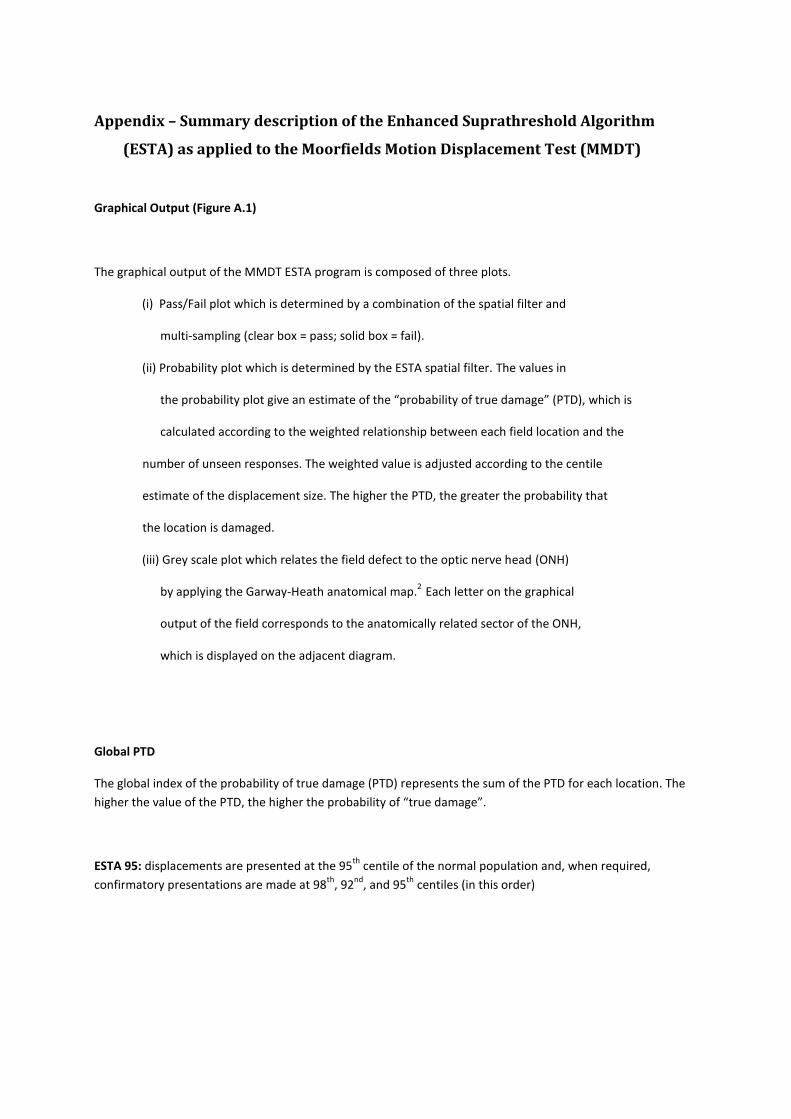
Appendix – Summary description of the Enhanced Suprathreshold Algorithm
(ESTA) as applied to the Moorfields Motion Displacement Test (MMDT)
Graphical Output (Figure A.1)
The graphical output of the MMDT ESTA program is composed of three plots.
(i) Pass/Fail plot which is determined by a combination of the spatial filter and
multi-sampling (clear box = pass; solid box = fail).
(ii) Probability plot which is determined by the ESTA spatial filter. The values in
the probability plot give an estimate of the “probability of true damage” (PTD), which is
calculated according to the weighted relationship between each field location and the
number of unseen responses. The weighted value is adjusted according to the centile
estimate of the displacement size. The higher the PTD, the greater the probability that
the location is damaged.
(iii) Grey scale plot which relates the field defect to the optic nerve head (ONH)
by applying the Garway-Heath anatomical map.2
Each letter on the graphical
output of the field corresponds to the anatomically related sector of the ONH,
which is displayed on the adjacent diagram.
Global PTD
The global index of the probability of true damage (PTD) represents the sum of the PTD for each location. The
higher the value of the PTD, the higher the probability of “true damage”.
ESTA 95: displacements are presented at the 95th
centile of the normal population and, when required,
confirmatory presentations are made at 98th
, 92nd
, and 95th
centiles (in this order)
9 Improving measurements in perimetry for glaucoma 2011
163
Figure A-1 Example of ESTA MMDT graphical output showing an upper hemifield defect (right eye).
General rules
All stimulus displacements (3 oscillations at 200 ms per cycle) are presented in randomised order The rules of the Pandora response algorithm are applied. Where a false response occurs the
displacement is represented within the randomised order of the test sequence.
Rules of the MMDT ESTA Spatial Filter
A spatial filter is applied to estimate the weighting array (WA) between each test location (TL). The ESTA spatial filter is static and the weightings are therefore only calculated once. Locations are clustered according to the anatomical entry of nerve fibre bundles into the optic nerve
head (ONH). The distance of each location to the ONH is traced. The angle between each primary test
TL relative to each of the secondary 31 TLs is calculated (ONHd). These values are integrated into the software through referencing a ready prepared look-up table which is derived from Figure A-2 (from Garway-Heath et al 2000).
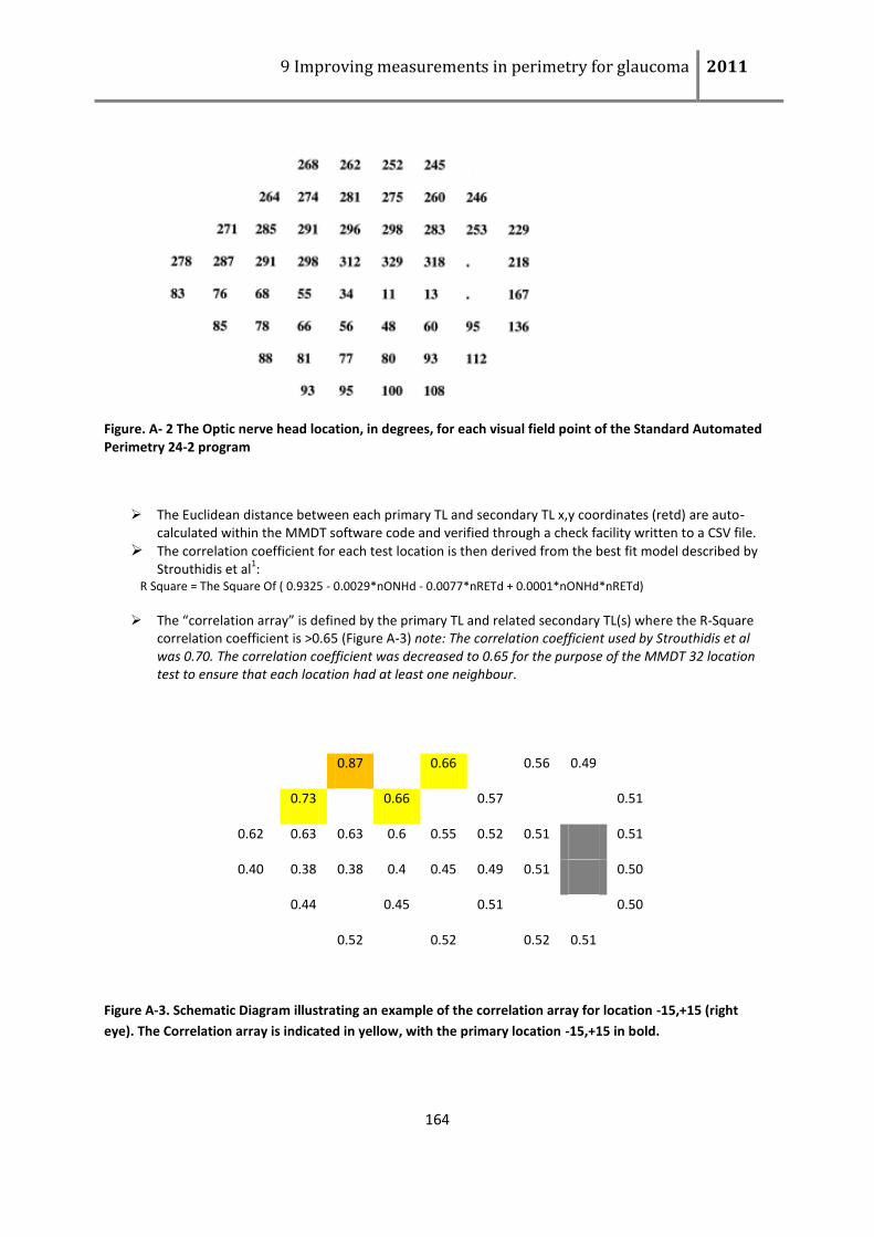
9 Improving measurements in perimetry for glaucoma 2011
164
Figure. A- 2 The Optic nerve head location, in degrees, for each visual field point of the Standard Automated Perimetry 24-2 program
The Euclidean distance between each primary TL and secondary TL x,y coordinates (retd) are auto-calculated within the MMDT software code and verified through a check facility written to a CSV file.
The correlation coefficient for each test location is then derived from the best fit model described by Strouthidis et al
1:
R Square = The Square Of ( 0.9325 - 0.0029*nONHd - 0.0077*nRETd + 0.0001*nONHd*nRETd)
The “correlation array” is defined by the primary TL and related secondary TL(s) where the R-Square correlation coefficient is >0.65 (Figure A-3) note: The correlation coefficient used by Strouthidis et al was 0.70. The correlation coefficient was decreased to 0.65 for the purpose of the MMDT 32 location test to ensure that each location had at least one neighbour.
0.87
0.66
0.56 0.49
0.73
0.66
0.57
0.51
0.62 0.63 0.63 0.6 0.55 0.52 0.51 0.51
0.40 0.38 0.38 0.4 0.45 0.49 0.51 0.50
0.44
0.45
0.51
0.50
0.52
0.52
0.52 0.51
Figure A-3. Schematic Diagram illustrating an example of the correlation array for location -15,+15 (right
eye). The Correlation array is indicated in yellow, with the primary location -15,+15 in bold.
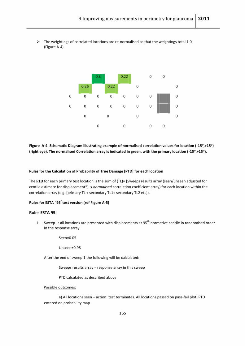
9 Improving measurements in perimetry for glaucoma 2011
165
The weightings of correlated locations are re-normalised so that the weightings total 1.0 (Figure A-4)
0.3
0.22
0 0
0.26
0.22
0
0
0 0 0 0 0 0 0 0
0 0 0 0 0 0 0 0
0
0
0
0
0
0
0 0
Figure A-4. Schematic Diagram illustrating example of normalised correlation values for location (-15⁰,+15⁰)
(right eye). The normalised Correlation array is indicated in green, with the primary location (-15⁰,+15⁰).
Rules for the Calculation of Probability of True Damage [PTD] for each location
The PTD for each primary test location is the sum of (TL)= [Sweeps results array (seen/unseen adjusted for
centile estimate for displacement*) x normalised correlation coefficient array) for each location within the
correlation array (e.g. [primary TL + secondary TL1+ secondary TL2 etc]).
Rules for ESTA “95” test version (ref Figure A-5)
Rules ESTA 95:
1. Sweep 1: all locations are presented with displacements at 95th
normative centile in randomised order In the response array:
Seen=0.05
Unseen=0.95
After the end of sweep 1 the following will be calculated:
Sweeps results array = response array in this sweep
PTD calculated as described above
Possible outcomes:
a) All locations seen – action: test terminates. All locations passed on pass-fail plot; PTD
entered on probability map

9 Improving measurements in perimetry for glaucoma 2011
166
b) > 10 locations unseen – action test terminates. Unseen locations failed on pass fail plot.
PTD entered on probability map
c) ≥1 ≤9 locations are missed: locations will be retested if they fall within the range L1 (lower
bound for sweep 1) to U1 (Upper bound for sweep 1) as specified in ini file.
Once a decision is taken not to test a location again, that decision is final. However the PTD for that
location will continue to be updated for subsequent sweeps. The location will not be re-tested even
if the updated PTD is within the boundaries for re-testing.
2. Sweeps 2 presents locations identified in 1c) with displacements at 98th
centile In the response array:
Seen=0.02
Unseen=0.98
After the end of sweep 2 the following will be calculated:
Sweeps results array = (response array1 + response array2)/n, where n is the number of
presentations made at that location
PTD calculated as described above
Actions:
If any of the following applies, the testing at that location terminates:
a) if both unseen
b) if both seen
c) if PTD >U2 (as specified in ini file)
d if PTD <L2 (as specified in ini file)
For each location, once a decision to not test it again has been made, that decision is final
3. Sweep 3 presents displacements at 92nd
centile

9 Improving measurements in perimetry for glaucoma 2011
167
In the response array:
Seen=0.08
Unseen=0.92
After the end of sweep 3 the following will be calculated:
Sweeps results array = (response array1 + response array2 + response array3)/n, where n is the
number of presentations made at that location
PTD calculated as described above
Actions:
If any of the following applies, the testing at that location terminates:
a) if seen in sweep 1, unseen in sweep 2 a. seen in sweep 3 (the pass/fail plot will record it as pass)
b) if unseen in sweep 2, seen in sweep 2 a. unseen in sweep 3 (the pass/fail plot will record it as fail)
c) if PTD >U3 (as specified in ini file) d) if PTD <L3 (as specified in ini file)
For each location, once a decision to not test it again has been made, that decision is final
4. sweep 4 presents displacements at 95th
centile In the response array:
Seen=0.05
Unseen=0.95
After the end of sweep 4 the following will be calculated:
Sweeps results array = (response array1 + response array2 + response array3 + response
array4)/n, where n is the number of presentations made at that location
PTD calculated as described above
Rules for the Pass-Fail graphical output for each location – 95 centile
Pass-Fail Rules (examples in the table below):
1. A location will be recorded as FAIL if one or all applies: a) PTD>U b) sweep 1 AND sweep 2 unseen c) two unseen in sweep 1, 3 or 4
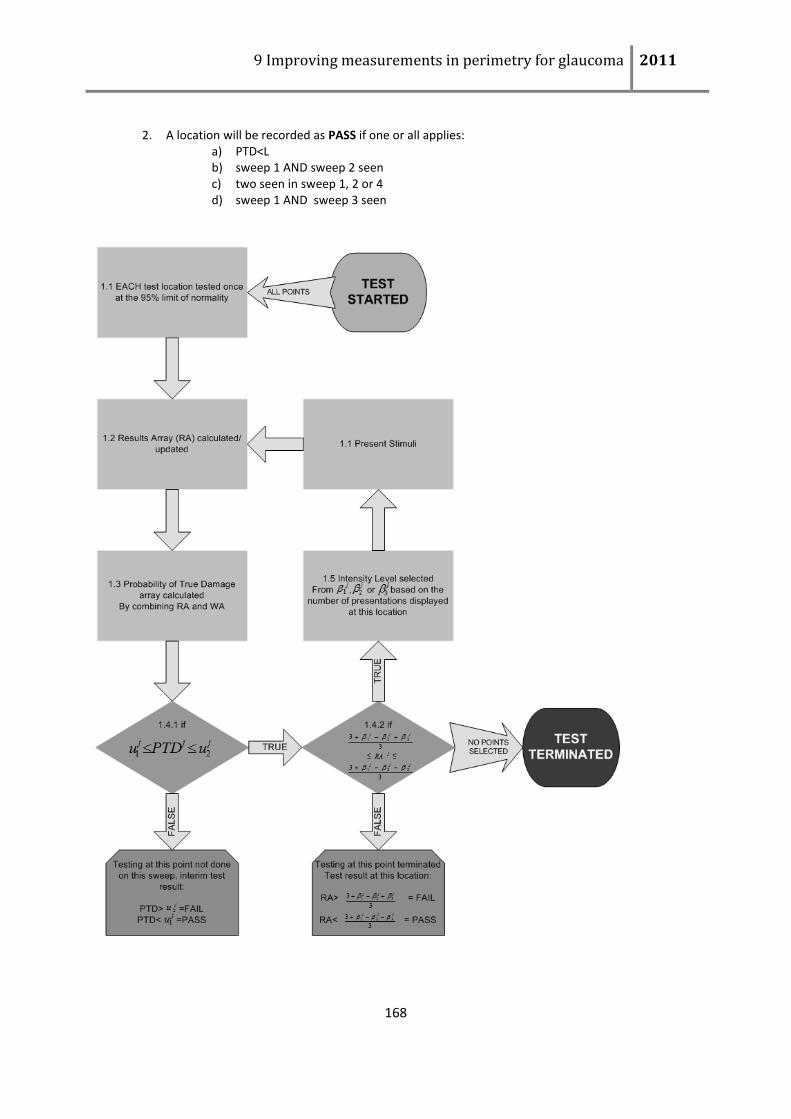
9 Improving measurements in perimetry for glaucoma 2011
168
2. A location will be recorded as PASS if one or all applies: a) PTD<L b) sweep 1 AND sweep 2 seen c) two seen in sweep 1, 2 or 4 d) sweep 1 AND sweep 3 seen

9 Improving measurements in perimetry for glaucoma 2011
169
Figure A-5 Detailed flow chart of ESTA, PTD denotes the probability of true damage, RA the results array, WA the
weighting array, the presentation intensity level on that sweep and
the upper and lower limits for retesting
at the j the location.
Table 1: Possible outcomes in the pass-fail graphical output.
Scenario Sweep 1 Sweep 2 Sweep 3 Sweep 4 Outcome
95% 98% 92% 95%
1 Seen (PTD<L1) Pass
2 Unseen
(PTD >U1) Fail
3 Unseen
(L1<PTD<U1) Unseen Fail
4 Seen
(L1<PTD<U1) Seen Pass
5 (a) Unseen
(L1<PTD<U1)
Seen
(PTD>U2) Fail
5 (b) Unseen
(L1<PTD<U1)
Seen
(PTD<L2) Pass
5 (c) Unseen
(L1<PTD<U1)
Seen
(PTD>U2) Unseen Fail
6 (a) Seen
(L1<PTD<U1)
Unseen
(PTD>U2) Fail
6 (b) Seen
(L1<PTD<U1)
Unseen
(PTD<L2) Pass
6 (c) Seen
(L1<PTD<U1)
Unseen
(L2<PTD<U2) Seen Pass
7 Unseen
(L1<PTD<U1)
Seen
(L2<PTD<U2)
Seen
(PTD>U3) Fail

9 Improving measurements in perimetry for glaucoma 2011
170
7 Unseen
(L1<PTD<U1)
Seen
(L2<PTD<U2)
Seen
(PTD<L3) Pass
7 Unseen
(L1<PTD<U1)
Seen
(L2<PTD<U2)
Seen
(L3<PTD<U3) Unseen Fail
8 Unseen
(L1<PTD<U1)
Seen
(L2<PTD<U2)
Seen
(PTD>U3) Fail
8 Unseen
(L1<PTD<U1)
Seen
(L2<PTD<U2)
Seen
(PTD<L3) Pass
8 Unseen
(L1<PTD<U1)
Seen
(L2<PTD<U2)
Seen
(L3<PTD<U3) Seen Pass
9 Seen
(L1<PTD<U1)
Unseen
(L2<PTD<U2)
Unseen
(PTD>U3) Fail
9 Seen
(L1<PTD<U1)
Unseen
(L2<PTD<U2)
Unseen
(PTD<L3) Pass
9 Seen
(L1<PTD<U1)
Unseen
(L2<PTD<U2)
Unseen
(L3<PTD<U3) Unseen Fail
10 Seen
(L1<PTD<U1)
Unseen
(L2<PTD<U2)
Unseen
(PTD>U3) Fail
10 Seen
(L1<PTD<U1)
Unseen
(L2<PTD<U2)
Unseen
(PTD<L3) Pass
10 Seen
(L1<PTD<U1)
Unseen
(L2<PTD<U2)
Unseen
(L3<PTD<U3) Seen Pass
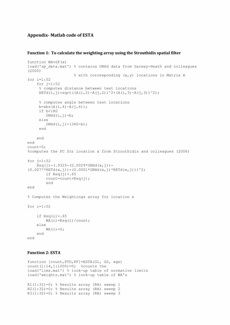
Appendix- Matlab code of ESTA
Function 1: To calculate the weighting array using the Strouthidis spatial filter
function WA=SF(x) load('sp_data.mat') % contains ONHd data from Garway-Heath and colleagues
(2000) % with corresponding (x,y) locations in Matrix A for i=1:52 for j=1:52 % computes distance between test locations RETd(i,j)=sqrt((A(i,2)-A(j,2))^2+(A(i,3)-A(j,3))^2);
% computes angle between test locations b=abs(A(i,4)-A(j,4)); if b<180 ONHd(i,j)=b; else ONHd(i,j)=(360-b); end
end end count=0; %computes the FC for location x from Strouthidis and colleagues (2006)
for j=1:52 Rsq(j)=(.9325-(0.0029*ONHd(x,j))-
(0.0077*RETd(x,j))+(0.0001*ONHd(x,j)*RETd(x,j)))^2; if Rsq(j)>.65 count=count+Rsq(j); end end
% Computes the Weightings array for location x
for i=1:52
if Rsq(i)>.65 WA(i)=Rsq(i)/count; else WA(i)=0; end end
Function 2: ESTA
function [count,PTD,PF]=ESTA(G1, G2, age) count(1:14,1:1000)=0; %counts the load('lims.mat') % look-up table of normative limits load('weights.mat') % look-up table of WA's
R1(1:32)=0; % Results array (RA) sweep 1 R2(1:32)=0; % Results array (RA) sweep 2 R3(1:32)=0; % Results array (RA) sweep 3
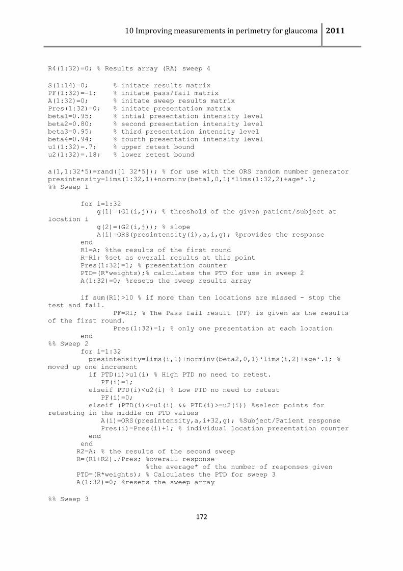
10 Improving measurements in perimetry for glaucoma 2011
172
R4(1:32)=0; % Results array (RA) sweep 4
S(1:14)=0; % initate results matrix PF(1:32)=-1; % initate pass/fail matrix A(1:32)=0; % initate sweep results matrix Pres(1:32)=0; % initate presentation matrix beta1=0.95; % intial presentation intensity level beta2=0.80; % second presentation intensity level beta3=0.95; % third presentation intensity level beta4=0.94; % fourth presentation intensity level u1(1:32)=.7; % upper retest bound u2(1:32)=.18; % lower retest bound
a(1,1:32*5)=rand([1 32*5]); % for use with the ORS random number generator presintensity=lims(1:32,1)+norminv(beta1,0,1)*lims(1:32,2)+age*.1; %% Sweep 1
for i=1:32 g(1)=(G1(i,j)); % threshold of the given patient/subject at
location i g(2)=(G2(i,j)); % slope A(i)=ORS(presintensity(i),a,i,g); %provides the response end R1=A; %the results of the first round R=R1; %set as overall results at this point Pres(1:32)=1; % presentation counter PTD=(R*weights);% calculates the PTD for use in sweep 2 A(1:32)=0; %resets the sweep results array
if sum(R1)>10 % if more than ten locations are missed - stop the
test and fail. PF=R1; % The Pass fail result (PF) is given as the results
of the first round. Pres(1:32)=1; % only one presentation at each location end %% Sweep 2 for i=1:32 presintensity=lims(i,1)+norminv(beta2,0,1)*lims(i,2)+age*.1; %
moved up one increment if PTD(i)>u1(i) % High PTD no need to retest. PF(i)=1; elseif PTD(i)<u2(i) % Low PTD no need to retest PF(i)=0; elseif (PTD(i)<=u1(i) && PTD(i)>=u2(i)) %select points for
retesting in the middle on PTD values A(i)=ORS(presintensity,a,i+32,g); %Subject/Patient response Pres(i)=Pres(i)+1; % individual location presentation counter end end R2=A; % the results of the second sweep R=(R1+R2)./Pres; %overall response- %the average* of the number of responses given PTD=(R*weights); % Calculates the PTD for sweep 3 A(1:32)=0; %resets the sweep array
%% Sweep 3
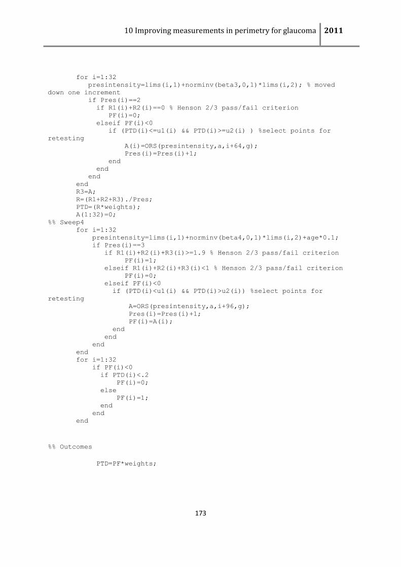
10 Improving measurements in perimetry for glaucoma 2011
173
for i=1:32 presintensity=lims(i,1)+norminv(beta3,0,1)*lims(i,2); % moved
down one increment if Pres(i)==2 if R1(i)+R2(i)==0 % Henson 2/3 pass/fail criterion PF(i)=0; elseif PF(i)<0 if (PTD(i)<=u1(i) && PTD(i)>=u2(i) ) %select points for
retesting A(i)=ORS(presintensity,a,i+64,g); Pres(i)=Pres(i)+1; end end end end R3=A; R=(R1+R2+R3)./Pres; PTD=(R*weights); A(1:32)=0; %% Sweep4 for i=1:32 presintensity=lims(i,1)+norminv(beta4,0,1)*lims(i,2)+age*0.1; if Pres(i)==3 if R1(i)+R2(i)+R3(i)>=1.9 % Henson 2/3 pass/fail criterion PF(i)=1; elseif R1(i)+R2(i)+R3(i)<1 % Henson 2/3 pass/fail criterion PF(i)=0; elseif PF(i)<0 if (PTD(i)<u1(i) && PTD(i)>u2(i)) %select points for
retesting A=ORS(presintensity,a,i+96,g); Pres(i)=Pres(i)+1; PF(i)=A(i); end end end end for i=1:32 if PF(i)<0 if PTD(i)<.2 PF(i)=0; else PF(i)=1; end end end
%% Outcomes
PTD=PF*weights;
References
AIRAKSINEN, P. J., DRANCE, S. M., DOUGLAS, G. R. & SCHULZER, M. (1985) Neuroretinal rim areas and visual field indices in glaucoma. Am J Ophthalmol, 99, 107-110.
ANDERSON, A. J. (2003a) Spatial resolution of the tendency-oriented perimetry algorithm. Invest Opthalmol Vis Sci, 44, 1962.
ANDERSON, A. J. (2003b) Utility of a dynamic termination criterion in the ZEST adaptive threshold method. Vis Res, 43, 165-170.
ANDERSON, A. J. & JOHNSON, C. A. (2006) Comparison of the ASA, MOBS, and ZEST threshold methods. Vis Res, 46, 2403-2411.
ANDERSON, A. J., JOHNSON, C. A., FINGERET, M., KELTNER, J. L., SPRY, P. G. D., WALL, M. & WERNER, J. S. (2005) Characteristics of the Normative Database for the Humphrey Matrix Perimeter. Invest Opthalmol Vis Sci, 46, 1540-1548.
ANDERSON, A. J. & MCKENDRICK, A. M. (2007) Quantifying Adaptation and Fatigue Effects in Frequency Doubling Perimetry. Invest Opthalmol Vis Sci, 48, 943-948.
ANDERSON, R. S. (1996) The selective effect of optical defocus on detection and resolution acuity in peripheral vision. Curr Eye Res, 15, 351-3.
ANDERSON, R. S. (2006) The psychophysics of glaucoma: Improving the structure/function relationship. Prog Retin Eye Res, 25, 79-97.
ANDERSON, R. S., DETKOVA, P. & O'BRIEN, C. (1995) Effect of temporal frequency and contrast on peripheral grating resolution. Curr Eye Res, 14, 1031-1033.
ANDERSON, R. S., REDMOND, T., MCDOWELL, D. R., BRESLIN, K. M. M. & ZLATKOVA, M. B. (2009) The Robustness of Various Forms of Perimetry to Different Levels of Induced Intraocular Stray Light. Invest Ophthalmol Vis Sci, 50, 4022-4028.
ANDERSON, R. S., ZLATKOVA, M. B. & BEIRNE, R. O. (2002) The contrast sensitivity function for detection and resolution of blue-on-yellow gratings in foveal and peripheral vision. Ophthalmic Physiol Opt, 22, 420-426.
ARAIE, M., ARAI, M., KOSEKI, N. & SUZUKI, Y. (1995) Influence of myopic refraction on visual field defects in normal tension and primary open angle glaucoma. Jpn J Ophthalmol, 39, 60-64.
ARMALY, M. F. (1969) The optic cup in the normal eye. Am J Ophthalmol, 68, 405-407. ARTAL, P., GUIRAO, A., BERRIO, E. & WILLIAMS, D. R. (2001) Compensation of corneal aberrations by
the internal optics in the human eye. J Vision, 1, 1-8. ARTES, P. H., HENSON, D. B. & CHAUDRY, S. J. (2002a) Pointwise pass/fail criteria in suprathreshold
perimetry. Perimetry Update, 283–291. ARTES, P. H., HENSON, D. B., HARPER, R. & MCLEOD, D. (2003) Multisampling Suprathreshold
Perimetry: A Comparison with Conventional Suprathreshold and Full-Threshold Strategies by Computer Simulation. Invest Ophthalmol Vis Sci, 44, 2582-2587.
ARTES, P. H., HUTCHISON, D. M., NICOLELA, M. T., LEBLANC, R. P. & CHAUHAN, B. C. (2005) Threshold and Variability Properties of Matrix Frequency-Doubling Technology and Standard Automated Perimetry in Glaucoma Invest Ophthalmol Vis Sci, 46, 2451-2457.
ARTES, P. H., IWASE, A., OHNO, Y., KITAZAWA, Y. & CHAUHAN, B. C. (2002b) Properties of perimetric threshold estimates from Full Threshold, SITA Standard, and SITA Fast strategies. Invest Ophthalmol Vis Sci, 43, 2654-2659.
ARTES, P. H., NICOLELA, M. T., AGOUMI, Y., SHARPE, G., CHAUHAN, B. C. & ST KITTS EYE STUDY GROUP (2009) The St Kitts Eye Study (SKES): Design and Initial Findings. Invest Ophthalmol Vis Sci (E-Abstract), 50, 4080-.
ASMAN, P. & HEIJL, A. (1992) Evaluation of methods for automated Hemifield analysis in perimetry. Arch Ophthalmol, 110, 820-826.

11 Improving measurements in perimetry for glaucoma 2011
175
ÅSMAN, P. & HEIJL, A. (1994) Diffuse visual field loss and glaucoma. Acta Ophthalmologica, 72, 303-308.
ASMAN, P., HEIJL, A., OLSSON, J. & ROOTZEN, H. (1992) Spatial analyses of glaucomatous visual fields; a comparison with traditional visual field indices. Acta Ophthalmologica, 70, 679-686.
AUTZEN, T. & WORK, K. (1990) The effect of learning and age on short-term fluctuation and mean sensitivity of automated static perimetry. Acta Ophthalmologica, 68, 327-330.
BEBIE, H., FANKHAUSER, F. & SPAHR, J. (1976) Static Perimetry: Accuracy and Fluctuations. Acta Ophthalmologica, 54, 339-349.
BEBIE, H., FLAMMER, J. & BEBIE, T. (1989) The cumulative defect curve: separation of local and diffuse components of visual field damage. Graefe's Arch Clin Exp Ophthalmol, 227, 9-12.
BELL, R. W. & O'BRIEN, C. (1997) Accuracy of referral to a glaucoma clinic. Ophthalmic Physiol Opt, 17, 7-11.
BENGTSSON, B. & HEIJL, A. (1999a) Comparing significance and magnitude of glaucomatous visual field defects using the SITA and Full Threshold strategies. Acta Ophthalmologica, 77, 143-6.
BENGTSSON, B. & HEIJL, A. (1999b) Inter-subject variability and normal limits of the SITA Standard, SITA Fast, and the Humphrey Full Threshold computerized perimetry strategies, SITA STATPAC. Acta Ophthalmologica, 77, 125-9.
BENGTSSON, B. & HEIJL, A. (2003) Normal intersubject threshold variability and normal limits of the SITA SWAP and full threshold SWAP perimetric programs. Invest Opthalmol Vis Sci, 44, 5029-34.
BENGTSSON, B., OLSSON, J., HEIJL, A. & ROOTZEN, H. (1997) A new generation of algorithms for computerized threshold perimetry, SITA. Acta Ophthalmologica, 75, 368-75.
BERGIN, C., GARWAY-HEATH, D. F. & CRABB, D. P. (2008) Evaluating the effect of the new alignment algorithm for longitudinal series of Heidelberg retina tomography images. Acta Ophthalmologica, 86, 207-14.
BERGIN, C., REDMOND, T., NATHWANI, N., VERDON-ROE, G. M., CRABB, D. P., ANDERSON, R. S. & GARWAY-HEATH, D. F. (2011) The effect of induced intraocular stray light on perimetric tests. Invest Opthalmol Vis Sci, 52, 3676-3682.
BERGIN, C., SINAPIS, D., SINAPIS, A., MOOSAVI, R., VERDON-ROE, G. M., CRABB, D. P. & GARWAY-HEATH, D. F. (2010a) Perimetry Instrument Comparison Study: Comparing the 'Screening' Strategies of Three Perimetry Devices to Discriminate Between Healthy and 'Glaucomatous' Eyes (Interim Results). Invest Ophthalmol Vis Sci (E-Abstract), 51, 5508-.
BERGIN, C., VERDON-ROE, G. M., SHARKAWI, E., CRABB, D. & GARWAY-HEATH, D. F. (2010b) ESTA a new screening strategy for glaucoma case-finding. Imaging and Perimetry Society Conference. Tenerife, Spain.
BIGGER, J. F. & BECKER, B. (1994) Cataracts and glaucoma. The effect of cataract extraction on visual fields. Am J Ophthalmol, 71, 335-340.
BLOMDAHL, S., CALISSENDORFF, B. M., TENGROTH, B. & WALLIN, O. (1997) Blindness in glaucoma patients. Acta Ophthalmologica, 75, 589-91.
BORISUTH, N., PHILLIPS, B. & KRUPIN, T. (1999) The risk profile of glaucoma filtration surgery. Curr Opin Ophthalmol, 10, 112.
BOSSUYT, P. M., REITSMA, J. B., BRUNS, D. E., GATSONIS, C. A., GLASZIOU, P. P., IRWIG, L. M., LIJMER, J. G., MOHER, D., RENNIE, D. & DE VET, H. C. W. (2003a) Towards complete and accurate reporting of studies of diagnostic accuracy: the STARD initiative. Clin Chem, 49, 1.
BOSSUYT, P. M., REITSMA, J. B., BRUNS, D. E., GATSONIS, C. A., IRWIG, L. M., MOHER, D., RENNIE, D., DE VET, H. C. W. & LIJMER, J. G. (2003b) The STARD statement for reporting studies of diadnostic accuracy: explanation and elaboration. Clin Chem, 49, 7-18.
BOURNE, R. R., FOSTER, P. J., BUNCE, C., PETO, T., HITCHINGS, R. A., KHAW, P. T., SEAH, S. K. & GARWAY-HEATH, D. F. (2008) The morphology of the optic nerve head in the Singaporean
11 Improving measurements in perimetry for glaucoma 2011
176
Chinese population (the Tanjong Pagar study): part 2--Biometric and systemic associations. Br J Ophthalmol, 92, 310-4.
BOWD, C., HAO, J., TAVARES, I. M., MEDEIROS, F. A., ZANGWILL, L. M., LEE, T. W., SAMPLE, P. A., WEINREB, R. N. & GOLDBAUM, M. H. (2008) Bayesian machine learning classifiers for combining structural and functional measurements to classify healthy and glaucomatous eyes. Invest Opthalmol Vis Sci, 49, 945-53.
BOWD, C., WEINREB, R. N., WILLIAMS, J. M. & ZANGWILL, L. M. (2000) The retinal nerve fiber layer thickness in ocular hypertensive, normal, and glaucomatous eyes with optical coherence tomography. Arch Ophthalmol, 118, 22-6.
BOWD, C., ZANGWILL, L., MEDEIROS, F., TAVARES, I., HOFFMANN, E., BOURNE, R., SAMPLE, P. & WEINREB, R. (2006) Structure-function relationships using confocal scanning laser ophthalmoscopy, optical coherence tomography, and scanning laser polarimetry. Invest Opthalmol Vis Sci (E-Abstract), 47, 2889.
BOWD, C., ZANGWILL, L. M., BERRY, C. C., BLUMENTHAL, E. Z., VASILE, C., SANCHEZ-GALEANA, C., BOSWORTH, C. F., SAMPLE, P. A. & WEINREB, R. N. (2001) Detecting early glaucoma by assessment of retinal nerve fiber layer thickness and visual function. Invest Opthalmol Vis Sci, 42, 1993-2003.
BOWLING, B., CHEN, S. & SALMON, J. (2005) Outcomes of referrals by community optometrists to a hospital glaucoma service. Br J Ophthalmol, 89, 1102.
BRANDT, J. D., BEISER, J. A., KASS, M. A. & GORDON, M. O. (2001) Central corneal thickness in the Ocular Hypertension Treatment Study (OHTS). Ophthalmology, 108, 1779-88.
BRINDLEY, G. & WESTHEIMER, G. (1965) The spatial properties of the human electroretinogram. J Physiol, 179, 518.
BRUSH, M. B. & CHEN, P. P. (2004) Test-retest variability in glaucoma patients tested with C-20-1 screening-mode frequency doubling technology perimetry. J Glaucoma, 13, 273.
BRUSINI, P., MIANI, F. & TOSONI, C. (2000) Corneal thickness in glaucoma: an important parameter? Acta Ophthalmol Scand Suppl, 41-2.
BUDENZ, D. L., FEUER, W. J. & ANDERSON, D. R. (1993) The effect of simulated cataract on the glaucomatous visual field. Ophthalmology, 100, 511-517.
BUNCE, C. & WORMALD, R. (2006) Leading causes of certification for blindness and partial sight in England & Wales. BMC Public Health, 6, 58.
BURK, R. O., VIHANNINJOKI, K., BARTKE, T., TUULONEN, A., AIRAKSINEN, P. J., VOLCKER, H. E. & KONIG, J. M. (2000) Development of the standard reference plane for the Heidelberg retina tomograph. Graefe's Arch Clin Exp Ophthalmol, 238, 375-84.
BURR, J. M., MOWATT, G., HERNANDEZ, R., SIDDIQUI, M. A., COOK, J., LOURENCO, T., RAMSAY, C., VALE, L., FRASER, C., AZUARA-BLANCO, A., DEEKS, J., CAIRNS, J., WORMALD, R., MCPHERSON, S., RABINDRANATH, K. & GRANT, A. (2007) The clinical effectiveness and cost-effectiveness of screening for open angle glaucoma: a systematic review and economic evaluation. Health Technology Assessment, 11, 1-190.
CALVO PEREZ, P., GIL ARRIBAS, L., FERRERAS, A., OTIN, S., ALTEMIR, I., FERNANDEZ, S., PABLO JULVEZ, L. & FUERTES, I. (2011) Relationship between flicker FDF perimetry and standard automated perimetry. Acta Ophthalmologica, 88, 0-0.
CAPRIOLI, J. & MILLER, J. M. (1989) Measurement of relative nerve fibre layer surface height in glaucoma. Ophthalmology, 96, 633-641.
CARRASCO, M. (2006) Covert attention increases contrast sensitivity: Psychophysical, neurophysiological and neuroimaging studies. Prog Brain Res, 154, 33-70.
CARRASCO, M., PENPECI-TALGAR, C. & ECKSTEIN, M. (2000) Spatial covert attention increases contrast sensitivity across the CSF: support for signal enhancement* 1. Vis Res, 40, 1203-1215.
11 Improving measurements in perimetry for glaucoma 2011
177
CARRILLO, M. M., ARTES, P. H., NICOLELA, M. T., LEBLANC, R. P. & CHAUHAN, B. C. (2005) Effect of cataract extraction on the visual fields of patients with glaucoma. Arch Ophthalmol, 123, 929-932.
CENTOFANTI, M., FOGAGNOLO, P., ODDONE, F., ORZALESI, N., VETRUGNO, M., MANNI, G. & ROSSETTI, L. (2008) Learning effect of Humphrey matrix frequency doubling technology perimetry in patients with ocular Hypertension. J Glaucoma, 17, 436.
CHANG, R. & BUDENZ, D. (2008a) Diagnosing glaucoma progression. Int Ophthalmol Clin, 48 (4), 13. CHANG, R. & BUDENZ, D. L. (2008b) New developments in optical coherence tomography for
glaucoma. Curr Opin Ophthalmol, 19, 127-35. CHATURVEDI, N., HEDLEY, W.-E. T. & DREYER, E. B. (1993) Lateral geniculate nucleus in glaucoma. Am
J Ophthalmol, 116, 182-8. CHAUHAN, B. C. (1996) Confocal scanning laser tomography. Canadian journal of ophthalmology, 31,
152-156. CHAUHAN, B. C., BLANCHARD, J. W., HAMILTON, D. C. & LEBLANC, R. P. (2000) Technique for
detecting serial topographic changes in the optic disc and peripapillary retina using scanning laser tomography. Invest Opthalmol Vis Sci, 41, 775-82.
CHAUHAN, B. C., DRANCE, S. M. & DOUGLAS, G. R. (1990) The use of visual field indices in detecting changes in the visual field in glaucoma. Invest Opthalmol Vis Sci, 31, 512-520.
CHAUHAN, B. C., DRANCE, S. M. & LAI, C. (1989) A cluster analysis for threshold perimetry. Graefe's Arch Clin Exp Ophthalmol, 227, 216-220.
CHAUHAN, B. C., GARWAY-HEATH, D. F., GONI, F. J., ROSSETTI, L., BENGTSSON, B., VISWANATHAN, A. C. & HEIJL, A. (2008) Practical recommendations for measuring rates of visual field change in glaucoma. Br J Ophthalmol, 92, 569-73.
CHAUHAN, B. C. & MCCORMICK, T. A. (1995) Effect of the cardiac cycle on topographic measurements using confocal scanning laser tomography. Graefe's Arch Clin Exp Ophthalmol, 233, 568-572.
CHAUHAN, B. C., MIKELBERG, F. S., ARTES, P. H., BALAZSI, A. G., LEBLANC, R. P., LESK, M. R., NICOLELA, M. T. & TROPE, G. E. (2010) Canadian Glaucoma Study: 3. Impact of Risk Factors and Intraocular Pressure Reduction on the Rates of Visual Field Change. Arch Ophthalmol, 128, 1249-1255.
CHAUHAN, B. C., TOMPKINS, J. D., LEBLANC, R. P. & MCCORMICK, T. A. (1993) Characteristics of frequency-of-seeing curves in normal subjects, patients with suspected glaucoma, and patients with glaucoma. Invest Opthalmol Vis Sci, 34, 3534-3540.
CHEN, P. P. (2003) Blindness in patients with treated open-angle glaucoma. Ophthalmology, 110, 726-33.
CHYLACK JR, L., WOLFE, J., SINGER, D., LESKE, M., BULLIMORE, M., BAILEY, I., FRIEND, J., MCCARTHY, D. & WU, S. (1993) The lens opacities classification system III. Arch Ophthalmol, 111, 831.
CIOFFI, G. A., MANSBERGER, S., SPRY, P., JOHNSON, C. & VAN BUSKIRK, E. M. (2000) Frequency doubling perimetry and the detection of eye disease in the community. Trans Am Ophthamol Soc, 98, 195.
CLEMENT, C. I., GOLDBERG, I., HEALEY, P. R. & GRAHAM, S. (2009) Humphrey matrix frequency doubling perimetry for detection of visual-field defects in open-angle glaucoma. Br J Ophthalmol, 93, 582-588.
COPT, R. P., THOMAS, R. & MERMOUD, A. (1999) Corneal thickness in ocular hypertension, primary open-angle glaucoma, and normal tension glaucoma. Arch Ophthalmol, 117, 14-6.
CRABB, D. P., EDGAR, D. F., FITZKE, F., MCNAUGHT, A. & WYNN, H. P. (1995) New approach to estimating variability in visual field data using an image processing technique. Br J Ophthalmol, 79, 213-217.
11 Improving measurements in perimetry for glaucoma 2011
178
CRABB, D. P., FITZKE, F. W., MCNAUGHT, A. I. & HITCHINGS, R. A. (1997) A profile of the spatial dependence of pointwise sensitivity across the glaucomatous visual field. Perimetry Update, 301-311.
CRAIG, J. E., BAIRD, P. N., HEALEY, D. L., MCNAUGHT, A. I., MCCARTNEY, P. J., RAIT, J. L., DICKINSON, J. L., ROE, L., FINGERT, J. H., STONE, E. M. & MACKEY, D. A. (2001) Evidence for genetic heterogeneity within eight glaucoma families, with the GLC1A Gln368STOP mutation being an important phenotypic modifier. Ophthalmology, 108, 1607-20.
CURCIO, C. A., ALLEN, K. A., SLOAN, K. R., LEREA, C. L., HURLEY, J. B., KLOCK, I. B. & MILAM, A. H. (1991) Distribution and morphology of human cone photoreceptors stained with anti-blue opsin. J Comp Neurol, 312, 610-24.
CZUDOWSKA, M., RAMDAS, W., WOLFS, R., HOFMAN, A., JONG, P., VINGERLING, J. & JANSONIUS, N. (2010) Incidence of Glaucomatous Visual Field Loss: A Ten-Year Follow-up from the Rotterdam Study. Ophthalmology, 117, 1705-1712.
DACEY, D. M. (1993) The mosaic of midget ganglion cells in the human retina. J Neurosci, 13, 5334-55.
DAVANGER, M., RINGVOLD, A. & BLIKA, S. (1991) The probability of having glaucoma at different IOP levels. Acta Ophthalmologica, 69, 565-568.
DE T PIERRE-FILHO, P., GOMES, P. R., PIERRE, E. T. & PIERRE, L. M. (2009) Learning effect in visual field testing of healthy subjects using Humphrey Matrix frequency doubling technology perimetry. Eye, 24, 851-856.
DE TARSO PONTE PIERRE FILHO, P., SCHIMITI, R. B., DE VASCONCELLOS, J. P. C. & COSTA, V. P. (2006) Sensitivity and specificity of frequency doubling technology, tendency oriented perimetry, SITA Standard and SITA Fast perimetry in perimetrically inexperienced individuals. Acta Ophthalmologica, 84, 345-350.
DE WAARD, P. W., IJSPEERT, J. K., VAN DEN BERG, T. J. & DE JONG, P. (1992) Intraocular light scattering in age-related cataracts. Invest Opthalmol Vis Sci, 33, 618-625.
DE WIT, G. C., FRANSSEN, L., COPPENS, J. E. & VAN DEN BERG, T. J. T. P. (2006) Simulating the straylight effects of cataracts. J Cataract Refract Surg, 32, 294-300.
DERMAN, C. (1957) Non-parametric up-and-down experimentation. Ann Math Stat, 28, 795-798. DIXON, W. & MOOD, A. (1948) A method for obtaining and analyzing sensitivity data. J Am Stat
Assoc, 43, 109-126. EFRON, B. (1979) Bootstrap methods: another look at the jackknife. Ann Statistics, 1-26. EFRON, B. (1981) Nonparametric standard errors and confidence intervals. Can J Statistics, 9, 139-
158. EFRON, B. & GONG, G. (1983) A leisurely look at the bootstrap, the jackknife, and cross-validation.
Am Statistician, 37, 36-48. EFRON, B. & TIBSHIRANI, R. (1991) Statistical data analysis in the computer age. Science, 253, 390. ENGER, C. & SOMMER, A. (1987) Recognizing glaucomatous field loss with the Humphrey STATPAC.
Arch Ophthalmol, 105, 1355-1357. ENOCH, J. M. & CAMPOS, E. C. (1980) New quantitative perimetric tests designed to evaluate
receptive- field- like properties in diseases of the retina and the optic nerve. Int Ophthalmol Clin, 20, 83-133.
ENOCH, J. M., SUNGA, R. N. & BACHMANN, E. (1970) Static perimetric technique believed to test receptive field properties. I. Extension of Westheimer's experiments on spatial interaction. Am J Ophthalmol, 70, 113-26.
FECHNER, G. T. (1860) Elemente der psychophysik, Breitkopf und Härtel. FITZKE, F. W., POINOOSAWMY, D., ERNST, W. & HITCHINGS, R. A. (1987) Peripheral displacement
thresholds in normals, ocular hypertensives and glaucoma. IN GREVE, E. & HEIJL, A. (Eds.) Perimetry Update 1986/1987. The Hague, The Netherlands, Kugler & Ghedini.
11 Improving measurements in perimetry for glaucoma 2011
179
FLAMMER, J., DRANCE, S. M., AUGUSTINY, L. & FUNKHOUSER, A. (1985) Quantification of glaucomatous visual field defects with automated perimetry. Invest Opthalmol Vis Sci, 26, 176-181.
FRANK, K. J. & DIECKERT, J. P. (1996) Diabetic eye disease: a primary care perspective. South Med J, 89, 463-470.
FRANSSEN, L., COPPENS, J. E. & VAN DEN BERG, T. J. T. P. (2006) Compensation Comparison Method for Assessment of Retinal Straylight. Invest Opthalmol Vis Sci, 47, 768-776.
FRANSSEN, L., TABERNERO, J., COPPENS, J. E. & VAN DEN BERG, T. J. T. P. (2007) Pupil Size and Retinal Straylight in the Normal Eye. Invest Opthalmol Vis Sci, 48, 2375-2382.
FRASER, S., BUNCE, C. & WORMALD, R. (1999) Risk factors for late presentation in chronic glaucoma. Invest Opthalmol Vis Sci, 40, 2251-7.
FRASER, S. & MANVIKAR, S. (2005) Glaucoma-the pathophysiology and diagnosis. Hosp Pharm Lond, 12, 251.
GARDINER, S., JOHNSON, C. & CIOFFI, G. (2005) Evaluation of the structure-function relationship in glaucoma. Invest Opthalmol Vis Sci, 46, 3712-3717.
GARDINER, S. K., CRABB, D. P., FITZKE, F. W. & HITCHINGS, R. A. (2004) Reducing noise in suspected glaucomatous visual fields by using a new spatial filter. Vis Res, 44, 839-48.
GARDINER, S. K. & DEMIREL, S. (2008) Assessment of patient opinions of different clinical tests used in the management of glaucoma. Ophthalmology, 115, 2127-2131.
GARWAY-HEATH, D. F. (2000) MD thesis: Correlation of structural and functional measurements in primary open angle glaucoma (optic disc morphology and psychophysics). University College London.
GARWAY-HEATH, D. F., CAPRIOLI, J., FITZKE, F. W. & HITCHINGS, R. A. (2000) Scaling the hill of vision: The physiological relationship between ganglion cell numbers and light sensitivity. Invest Opthalmol Vis Sci, 41, 1774-1782.
GARWAY-HEATH, D. F., HOLDER, G. E., FITZKE, F. W. & HITCHINGS, R. A. (2002) Relationship between electrophysiological, psychophysical, and anatomical measurements in glaucoma. Invest Opthalmol Vis Sci, 43, 2213-20.
GARWAY-HEATH, D. F., RUDNICKA, A. R., LOWE, T., FOSTER, P. J., FITZKE, F. W. & HITCHINGS, R. A. (1998) Measurement of optic disc size: equivalence of methods to correct for ocular magnification. Br J Ophthalmol, 82, 643-9.
GEDDE, S., HERNDON, L., BRANDT, J., BUDENZ, D., FEUER, W. & SCHIFFMAN, J. (2007a) Surgical complications in the Tube Versus Trabeculectomy Study during the first year of follow-up. Am J Ophthalmol, 143, 23-31.
GEDDE, S., SCHIFFMAN, J., FEUER, W., HERNDON, L., BRANDT, J. & BUDENZ, D. (2007b) Treatment outcomes in the tube versus trabeculectomy study after one year of follow-up. Am J Ophthalmol, 143, 9-22.
GIL, A. (2011) A comparison of perimetric results with standard automated perimetry and HEP perimetry in a group of glaucomatous patients. Acta Ophthalmologica, 88, 0-0.
GILMORE, E. D., HUDSON, C., NRUSIMHADEVARA, R. K. & HARVEY, P. T. (2005) Frequency of seeing characteristics of the short wavelength sensitive visual pathway in clinically normal subjects and diabetic patients with focal sensitivity loss. Br J Ophthalmol, 89, 1462-7.
GLOVINSKY, Y., QUIGLEY, H. A. & PEASE, M. E. (1993) Foveal ganglion cell loss is size dependent in experimental glaucoma. : Invest Ophthalmol Vis Sci, 34, 395-400.
GREENFIELD, D. S. & WEINREB, R. N. (2008) Role of optic nerve imaging in glaucoma clinical practice and clinical trials. Am J Ophthalmol, 145, 598-603.
HARVEY, L. (1997) Efficient estimation of sensory thresholds with ML-PEST. Spatial Vision, 11, 121-128.
11 Improving measurements in perimetry for glaucoma 2011
180
HARWERTH, R., CARTER-DAWSON, L., SHEN, F., SMITH, E. & CRAWFORD, M. (1999) Ganglion cell losses underlying visual field defects from experimental glaucoma. Invest Opthalmol Vis Sci, 40, 2242-2250.
HARWERTH, R. S., CARTER-DAWSON, L., SMITH, E. L., 3RD, BARNES, G., HOLT, W. F. & CRAWFORD, M. L. (2004) Neural losses correlated with visual losses in clinical perimetry. Invest Opthalmol Vis Sci, 45, 3152-60.
HARWERTH, R. S. & QUIGLEY, H. A. (2006) Visual field defects and retinal ganglion cell losses in patients with glaucoma. Arch Ophthalmol, 124, 853-9.
HAYASHI, K., HAYASHI, H., NAKAO, F. & HAYASHI, F. (2001) Influence of cataract surgery on automated perimetry in patients with glaucoma. Am J Ophthalmol, 132, 41-46.
HEIJL, A. (1976) Automatic perimetry in glaucoma visual field screening. Graefe's Arch Clin Exp Ophthalmol, 200, 21-37.
HEIJL, A. (1977) Computer test logics for automatic perimetry. Acta Ophthalmologica, 55, 837-853. HEIJL, A. (1985a) Computerised perimetry. Trans Ophthalmol Soc UK, 104, 76-87. HEIJL, A. (1985b) The Humphrey Field Analyser: Concepts and clinical results. Doc Ophthalmol, 43,
55-64. HEIJL, A. & ASMAN, P. (1989) Clustering of depressed points in the normal visual field. Perimetry
Update. Kugler & Ghedini. HEIJL, A. & DRANCE, S. M. (1980) Computerized profile perimetry in glaucoma. Arch Ophthalmol, 98,
2199-201. HEIJL, A. & KRAKAU, C. (1975a) An automatic static perimeter, design and pilot study. Acta
Ophthalmologica, 53, 293-310. HEIJL, A. & KRAKAU, C. E. T. (1975b) An automatic perimeter for glaucoma visual field screening and
control. Graefe's Arch Clin Exp Ophthalmol, 197, 13. HEIJL, A., LINDGREN, A. & LINDGREN, G. (1989) Inter-point correlations of deviations of threshold
values in normal and glaucomatous visual fields. Perimetry Update. Kugler & Ghedini. HEIJL, A., LINDGREN, G. & OLSSON, J. (1987) Normal variability of static perimetric threshold values
across the central visual field. Arch Ophthalmol, 105, 1544-1549. HEIJL, A. & PATELLA, V. M. (2002) Essential Perimetry, Carl Zeiss Meditec. HENSON, D., SPENCER, A., HARPER, R. & CADMAN, E. (2003) Community refinement of glaucoma
referrals. Eye, 17, 21-26. HENSON, D. B. (1993) Visual Fields., Oxford, Oxford University Press. HENSON, D. B. & ARTES, P. H. (2002) New developments in supra-threshold perimetry. Ophthalmic
Physiol Opt, 22, 463. HENSON, D. B., CHAUDRY, S., ARTES, P. H., FARAGHER, E. B. & ANSONS, A. (2000) Response
Variability in the Visual Field: Comparison of Optic Neuritis, Glaucoma, Ocular Hypertension, and Normal Eyes. Invest Ophthalmol Vis Sci, 41, 417-421.
HENSON, D. B. & EMUH, T. (2009) Measuring Patient Vigilance During Perimetry; The Pupillary Fatigue Index. Invest Ophthalmol Vis Sci, 50, 6195-.
HENSON, D. B. & EMUH, T. (2009) Measuring Patient Vigilance During Perimetry; The Pupillary Fatigue Index. Invest Ophthalmol Vis Sci, 50, 6195-.
HENSON, D. B. & EMUH, T. (2010) Monitoring Vigilance during Perimetry by Using Pupillography Invest Ophthalmol Vis Sci, 51(7), 3540-3543.
HENSON, D. B., SPENCELEY, S. E. & BULL, D. R. (1997) Artificial neural network analysis of noisy visual field data in glaucoma. Artif Intell Med, 10, 99-113.
HENSON, D. B., SPRY, P. G., SPENCER, I. C. & SPARROW, J. M. (1998) Variability in glaucomatous visual fields: implications for shared care schemes. Ophthalmic Physiol Opt, 18, 120-5.
11 Improving measurements in perimetry for glaucoma 2011
181
HERNANDEZ, R., RABINDRANATH, K., FRASER, C., VALE, L., BLANCO, A. A. & BURR, J. M. (2008) Screening for open angle glaucoma: systematic review of cost-effectiveness studies. J Glaucoma, 17, 159-68.
HERSE, P. R. (1992) Factors influencing normal perimetric thresholds obtained using the Humphrey Field Analyzer. Invest Opthalmol Vis Sci, 33, 611-7.
HILL, A. B. (1966) Principles of Medical Statistics, Lancet. HOOD, D. & KARDON, R. (2007) A framework for comparing structural and functional measures of
glaucomatous damage. Prog Retin Eye Res, 26, 688-710. HOOD, D. C., ANDERSON, S. C., WALL, M. & KARDON, R. H. (2007) Structure versus function in
glaucoma: an application of a linear model. Invest Opthalmol Vis Sci, 48, 3662. HUBEL, D. H. & WIESEL, T. N. (1960) Receptive fields of optic nerve fibres in the spider monkey. J
Physiol, 154, 572-580. HYLTON, C., CONGDON, N., FRIEDMAN, D., KEMPEN, J., QUIGLEY, H., BASS, E. & JAMPEL, H. (2003)
Cataract after glaucoma filtration surgery* 1. Am J Ophthalmol, 135, 231-232. IESTER, M., MERMOUD, A. & SCHNYDER, C. (2000) Frequency doubling technique in patients with
ocular hypertension and glaucoma: correlation with octopus perimeter indices. Ophthalmology, 107, 288-94.
IESTER, M., MIKELBERG, F. S. & DRANCE, S. M. (1997) The effect of optic disc size on diagnostic precision with the Heidelberg retina tomograph. Ophthalmology, 104, 545-8.
IJSPREET, J. K., DE WAARD, P. W. T., VAN DEN BERG, T. J. & DE JONG, P. (1990) The intraocular straylight function in 129 healthy volunteers: dependence on angle, age and pigmentation. Vis Res, 30, 699-707.
JOHNSON, C. A., ADAMS, C. W. & LEWIS, R. A. (1988) Fatigue effects in automated perimetry. Applied Optics, 27, 1030-7.
JOHNSON, C. A., BRANDT, J. D., KHONG, A. M. & ADAMS, A. J. (1995) Short-wavelength automated perimetry in low-, medium-, and high-risk ocular hypertensive eyes. Initial baseline results. Arch Ophthalmol, 113, 70-76.
JOHNSON, C. A., DEMIREL, S., ANDERSON, A. J., CHAUHAN, B. C., FINGERET, M. & SPRY, P. G. D. (2004) Detection of Glaucomatous Visual Field Loss Using the Humphrey Matrix Frequency Doubling Technology (FDT) Perimeter. Invest Ophthalmol Vis Sci (E-Abstract), 45, 3470-3470.
JOHNSON, C. A., KELTNER, J. L. & BALESTRERY, F. G. (1979) Suprathreshold static perimetry in glaucoma and other optic nerve disease. Ophthalmology, 86, 1278-1286.
KAERNBACH, C. (1991) Simple adaptive testing with the weighted up-down method. Perception & psychophysics, 49, 227-229.
KAERNBACH, C. (2001) Slope bias of psychometric functions derived from adaptive data. Percept Psychophys, 63, 1389-98.
KATZ, J. (2000) A comparison of the pattern- and total deviation-based Glaucoma Change Probability programs. Invest Opthalmol Vis Sci, 41, 1012-6.
KATZ, J. & SOMMER, A. (1986) Asymmetry and variation in the normal hill of vision. Arch Ophthalmol, 104, 65-68.
KELLY, D. H. (1966) Frequency doubling in visual responses. JOSA, 56, 1628-1632. KELLY, D. H. (1981) Nonlinear visual responses to flickering sinusoidal gratings. J Opt Soc Am, 71,
1051-5. KIM, D. Y., SUNG, K. R., KANG, S. Y., CHO, J. W., LEE, K. S., PARK, S. B., KIM, S. T. & KOOK, M. S. (2009)
Characteristics and reproducibility of anterior chamber angle assessment by anterior-segment optical coherence tomography. Acta Ophthalmologica, In press, 1-7.
KING-SMITH, P., GRIGSBY, S., VINGRYS, A., BENES, S. & SUPOWIT, A. (1994) Efficient and unbiased modifications of the QUEST threshold method: theory, simulations, experimental evaluation and practical implementation. Vis Res, 34, 885-912.
11 Improving measurements in perimetry for glaucoma 2011
182
KLEIN, B. E., KLEIN, R. & LINTON, K. L. (1992) Intraocular pressure in an American community. The Beaver Dam Eye Study. Invest Opthalmol Vis Sci, 33, 2224-2228.
KOCH, P., ROULIER, A. & FRANKHAUSER, F. (1972) Perimetry information theoretical basis for its automation. Vis Res, 12, 1619.
KONSEVICH, L., TYLER, C., (1999) Bayesian adaptive estimation of psychometric slope and threshold Vis Res, 39, 2729-2737
KOTECHA, A., WHITE, E., SCHLOTTMANN, P. & GARWAY-HEATH, D. (2010) Intraocular pressure measurement precision with the Goldmann applanation, dynamic contour, and ocular response analyzer tonometers. Ophthalmology, 117, 730-737.
KOTECHA, A., WHITE, E. T., SHEWRY, J. M. & GARWAY-HEATH, D. F. (2005) The relative effects of corneal thickness and age on Goldmann applanation tonometry and dynamic contour tonometry. Br J Ophthalmol, 89, 1572-5.
KREMMER, S., GARWAY-HEATH, D. F., DE CILLA, S., STEUHL, K. P. & SELBACH, J. M. (2003) Influence of cataract surgery with implantation of different intraocular lenses on scanning laser tomography and polarimetry. Am J Ophthalmol, 136, 1016-21.
KUZIN, A., VARMA, R., REDDY, H., TORRES, M. & AZEN, S. (2010) Ocular Biometry and Open-Angle Glaucoma: The Los Angeles Latino Eye Study. Ophthalmology, 117, 1713-1719.
LAM, B. L., ALWARD, W. L. & KOLDER, H. E. (1991) Effect of cataract on automated perimetry. Ophthalmology, 98, 1066-1070.
LAMPARTER, J., SCHULZE, A., SCHUFF, A. C., BERRES, M., PFEIFFER, N. & HOFFMANN, E. M. (2011) Learning Curve and Fatigue Effect of Flicker Defined Form Perimetry. Am J Ophthalmol, In press.
LANGMAN, M., LANCASHIRE, R., CHENG, K. & STEWART, P. (2005) Systemic hypertension and glaucoma: mechanisms in common and co-occurrence. Br J Ophthalmol, 89, 960.
LEVITT, H. (1971) Transformed up-down methods in psychoacoustics. J Acoust Soc Am, 49, 467–477. LIEBERMAN, H. & PENTLAND, A. (1982) Microcomputer-based estimation of psychophysical
thresholds: The best PEST. Behavior Research Methods & Instrumentation, 14, 21-25. LOCKWOOD, A., KIRWAN, J. & ASHLEIGH, Z. Optometrists referrals for glaucoma assessment: a
prospective survey of clinical data and outcomes. Eye, 24, 1515-1519. LY, T., GUPTA, N., WEINREB, R., KAUFMAN, P. & YÜCEL, Y. (2011) Dendrite Plasticity in the Lateral
Geniculate Nucleus in Primate Glaucoma. Vis Res, 51, 243-250. MALIK, R., SWANSON, W. H. & GARWAY-HEATH, D. F. (2006) Development and evaluation of a linear
staircase strategy for the measurement of perimetric sensitivity. Vis Res, 46, 2956-67. MANSBERGER, S. L., JOHNSON, C. A. & CIOFFI, G. A. (2007) The results of screening frequency
doubling technology perimetry in different locations of the community. J Glaucoma, 16, 73. MARRA, G. & FLAMMER, J. (1991) The learning and fatigue effect in automated perimetry. Graefe's
Arch Clin Exp Ophthalmol, 229, 501-504. MATSUMOTO, C., OGAWA, T., SUZUMURA, H., INOUE, H. & KIMURA, N. (1997) Influences of
cataracts on glaucomatous visual field changes. Perimetry Update, 1997, 139-145. MCKENDRICK, A. & TURPIN, A. (2005a) Combining perimetric suprathreshold and threshold
procedures to reduce measurement variability in areas of visual field loss. Optom Vis Sci, 82, 43.
MCKENDRICK, A. M., ANDERSON, A. J., JOHNSON, C. A. & FORTUNE, B. (2003) Appearance of the Frequency Doubling Stimulus in Normal Subjects and Patients with Glaucoma. Invest Opthalmol Vis Sci, 44, 1111-1116.
MCKENDRICK, A. M., BADCOCK, D. R. & MORGAN, W. H. (2004) Psychophysical measurement of neural adaptation abnormalities in magnocellular and parvocellular pathways in glaucoma. Invest Opthalmol Vis Sci, 45, 1846.
11 Improving measurements in perimetry for glaucoma 2011
183
MCKENDRICK, A. M. & TURPIN, A. (2005b) Advantages of terminating Zippy Estimation by Sequential Testing (ZEST) with dynamic criteria for white-on-white perimetry. Optom Vis Sci, 82, 981.
MEMBREY, L. & FITZKE, F. (2001) Effect of Lens Opacity on White-On-White Perimetry, Frequency Doubling Perimetry and Motion Detection Perimetry. Perimetry Update, 2001, 259-266.
MEMBREY, L., KOGURE, S. & FITZKE, F. (1999) A Comparison of the Effects of Neutral Density Filters and Diffusing Filters on Motion Detection Perimetry, White-On-White Perimetry and Frequency Doubling Perimetry. Perimetry Update, 999, 75-83.
MIKELBERG, F. S., PARFITT, C. M., SWINDALE, N. V., GRAHAM, S. L., DRANCE, S. M. & GOSINE, R. (1995) Ability of the Heidelberg Retina Tomograph to detect early glaucomatous visual field loss. J Glaucoma, 4, 242-247.
MILLER, G. (1956) The magic number seven, plus or minus two: Some limits on our capacity for processing information. Psychol Rev, 63, 81-97.
MITCHELL, P., ROCHTCHINA, E., LEE, A. J. & WANG, J. J. (2002) Bias in self-reported family history and relationship to glaucoma: the Blue Mountains Eye Study. Ophthalmic Epidemiol, 9, 333-45.
MOOSAVI, R. (In submission; MD Thesis) Normative database for the multi-location Moorfields Motion Displacement Test. Institute of Ophthalmology. London, University College London.
MORALES, J., WEITZMAN, M. & GONZÁLEZ DE LA ROSA, M. (2000) Comparison between tendency-oriented perimetry (TOP) and Octopus threshold perimetry. Ophthalmology, 107, 134-142.
MORGAN, J. E., WALDOCK, A., JEFFERY, G. & COWEY, A. (1998) Retinal nerve fibre layer polarimetry: histological and clinical comparison. Br J Ophthalmol, 82, 684-90.
MOSS, I. D., WILD, J. M. & WHITAKER, D. J. (1995) The influence of age-related cataract on blue-on-yellow perimetry. Invest Opthalmol Vis Sci, 36, 764-773.
MOWATT, G., BURR, J. M., COOK, J. A., SIDDIQUI, M. A., RAMSAY, C. R., FRASER, C., AZUARA-BLANCO, A. & DEEKS, J. J. (2008) Screening tests for detecting open angle glaucoma: systematic review and meta-analysis. Invest Opthalmol Vis Sci, 9, 9.
MUNOZ, B., WEST, S. K., RUBIN, G. S., SCHEIN, O. D., QUIGLEY, H. A., BRESSLER, S. B. & BANDEEN-ROCHE, K. (2000) Causes of blindness and visual impairment in a population of older Americans: The Salisbury Eye Evaluation Study. Arch Ophthalmol, 118, 819-25.
MYINT, J., EDGAR, D., KOTECHA, A., MURDOCH, I. & LAWRENSON, J. (2010) Barriers perceived by UK-based community optometrists to the detection of primary open angle glaucoma. Ophthalmic Physiol Opt, 30, 847-853.
MYINT, J., EDGAR, D., KOTECHA, A., MURDOCH, I. & LAWRENSON, J. (2011) A national survey of diagnostic tests reported by UK community optometrists for the detection of chronic open angle glaucoma. Ophthalmic Physiol Opt, In press.
NEHMAD, L. & MADONNA, R. J. (2008) Optimizing the use of frequency doubling technology perimetry in community vision screenings. Optom Vis Sci, 85, 559.
OLSSON, J., HEIJL, A., BENGTSSON, B. & ROOTZEN, H. (1993) Frequency-of-seeing in computerised perimetry. Perimetry Update, 551-556.
OLSSON, J. & ROOTZÉN, H. (1994) An image model for quantal response analysis in perimetry. Scand J Stat, 375-387.
ORGÜL S, KAISER HJ, FLAMMER J & P, G. (1995) Systemic blood pressure and capillary blood-cell velocity in glaucoma patients: a preliminary study. Eur J Ophthalmol, 5, 88-91.
ORGUL, S., CIOFFI, G. A., BACON, D. R. & VAN BUSKIRK, E. M. (1996) Sources of variability of topometric data with a scanning laser ophthalmoscope. Arch Ophthalmol, 114, 161-164.
PATEL, U., MURDOCH, I. & THEODOSSIADES, J. (2005) Glaucoma detection in the community: does ongoing training of optometrists have a lasting effect? Eye, 20, 591-594.
PATTERSON, A. J., GARWAY-HEATH, D. F., STROUTHIDIS, N. G. & CRABB, D. P. (2005) A new statistical approach for quantifying change in series of retinal and optic nerve head topography images. Invest Opthalmol Vis Sci, 46, 1659-67.
11 Improving measurements in perimetry for glaucoma 2011
184
PENTLAND, A. (1980) Maximum likelihood estimation: the best PEST. Perception & psychophysics, 28, 377.
PERERA, S., WONG, T., TAY, W., FOSTER, P., SAW, S. & AUNG, T. (2010) Refractive Error, Axial Dimensions, and Primary Open-Angle Glaucoma: The Singapore Malay Eye Study. Arch Ophthalmol, 128, 900.
POKORNY, J., SMITH, V. & LUTZE, M. (1987) Aging of the human lens. Applied Optics, 26, 1437-1440. POSNER, M. (1980) Orienting of attention. The Quarterly journal of experimental psychology, 32, 3-
25. QUAID, P. T. & FLANAGAN, J. G. (2005) Defining the limits of flicker defined form: effect of stimulus
size, eccentricity and number of random dots. Vis Res, 45, 1075-1084. QUIGLEY, H. (1998) Current and future approaches to glaucoma screening. J Glaucoma, 7, 210. QUIGLEY, H. A. (1999) Proportion of those with open-angle glaucoma who become blind [letter;
comment]. Ophthalmology, 106, 2039-41. QUIGLEY, H. A., ADDICKS, E. M. & GREEN, W. R. (1982) Optic Nerve Damage in Human Glaucoma - III.
Quantitative Correlation of Nerve Fiber Loss and Visual Field Defect in Glaucoma, Ischemic Neuropathy, Papilledema, and Toxic Neuropathy. Arch Ophthalmol, 100, 135-146.
QUIGLEY, H. A. & BROMAN, A. T. (2006) The number of people with glaucoma worldwide in 2010 and 2020. Br J Ophthalmol, 90, 262-7.
QUIGLEY, H. A., DUNKELBERGER, G. R. & GREEN, W. R. (1988) Chronic human glaucoma causing selectively greater loss of large optic nerve fibers. Ophthalmology, 95, 357-63.
QUIGLEY, H. A., FRIEDMAN, D. S. & HAHN, S. R. (2007) Evaluation of practice patterns for the care of open-angle glaucoma compared with claims data: the Glaucoma Adherence and Persistency Study. Ophthalmology, 114, 1599-606.
QUIGLEY, H. A., SANCHEZ, R. M., DUNKELBERGER, G. R., L'HERNAULT, N. L. & BAGINSKI, T. A. (1987) Chronic glaucoma selectively damages large optic nerve fibers. Invest Ophthalmol Vis Sci, 28, 913-20.
QURESHI, I. A. (1995) Age and intraocular pressure: how are they correlated? JPMA J Pak Med Assoc, 45, 150-152.
RACETTE, L., MEDEIROS, F. A., ZANGWILL, L. M., NG, D., WEINREB, R. N. & SAMPLE, P. A. (2008) Diagnostic Accuracy of the Matrix 24-2 and Original N-30 Frequency-Doubling Technology Tests Compared with Standard Automated Perimetry. Invest Opthalmol Vis Sci, 49, 954-960.
ROBBINS, H. & MONRO, S. (1951) A stochastic approximation method. Ann Math Stat, 22, 400-407. ROBIN, A., NOVACK, G., COVERT, D., CROCKETT, R. & MARCIC, T. (2007) Adherence in glaucoma:
objective measurements of once-daily and adjunctive medication use. Am J Ophthalmol, 144, 533-540.
ROOTZÉN, H. & OLSSON, J. (2006) On the influence of the prior distribution in image reconstruction. Comp Stat, 21, 431-444.
RUDDOCK, K. H. (1965) The effect of age upon colour vision. II. Changes with age in light transmission of the ocular media. Vis Res, 5, 47.
SAID, F. S. & WEALE, R. A. (1959) The variation with age of the spectral transmissivity of the living human crystalline lens. Gerontologia, 3, 213.
SAMPLE, P. A., ESTERSON, F. D., WEINREB, R. N. & BOYNTON, R. M. (1988) The aging lens: in vivo assessment of light absorption in 84 human eyes. Invest Opthalmol Vis Sci, 29, 1306-1311.
SCHAUMBERGER, M., SCHAFER, B. & LACHENMAYR, B. J. (1995) Glaucomatous visual fields. FASTPAC versus full threshold strategy of the Humphrey Field Analyzer. Invest Opthalmol Vis Sci, 36, 1390-1397.
SHAH, N. N., BOWD, C., MEDEIROS, F. A., WEINREB, R. N., SAMPLE, P. A., HOFFMANN, E. M. & ZANGWILL, L. M. (2006) Combining structural and functional testing for detection of glaucoma. Ophthalmology, 113, 1593-602.
11 Improving measurements in perimetry for glaucoma 2011
185
SHAH, S., CHATTERJEE, A., MATHAI, M., KELLY, S. P., KWARTZ, J., HENSON, D. & MCLEOD, D. (1999) Relationship between corneal thickness and measured intraocular pressure in a general ophthalmology clinic. Ophthalmology, 106, 2154-60.
SHELDRICK, J. H., NG, C., AUSTIN, D. J. & ROSENTHAL, A. R. (1994) An analysis of referral routes and diagnostic accuracy in cases of suspected glaucoma. Ophthalmic Epidemiol, 1, 31-9.
SHIU, L. & PASHLER, H. (1995) Spatial attention and vernier acuity. Vis Res, 35, 337-343. SIDDIQUI, M., AZUARA-BLANCO, A. & NEVILLE, S. (2005) Effect of cataract extraction on frequency
doubling technology perimetry in patients with glaucoma. Br J Ophthalmol, 89, 1569-1571. SIDDIQUI, M., KHAIRY, H. & AZUARA-BLANCO, A. (2007) Effect of Cataract Extraction on SITA
Perimetry in Patients With Glaucoma. J Glaucoma, 16, 205. SINAPIS, D., SINAPIS, A., BERGIN, C., MOOSAVI, R., RUSSELL, R. A., VERDON-ROE, G. M., BALIAN, C.,
FLANAGAN, J., CRABB, D. P. & GARWAY-HEATH, D. F. (2010) Perimetry Instrument Comparison Study: Comparing the Diagnostic Performance of Four Threshold Perimetry Tests to Discriminate Between Healthy and 'Glaucomatous' Eyes (Interim Analysis). Invest Ophthalmol Vis Sci (E-Abstract), 51, 5504-.
SOMMER, A. (1989) Intraocular pressure and glaucoma. Am J Ophthalmol, 107, 186-8. SOMMER, A. & TIELSCH, J. (2008) Blood Pressure, Perfusion Pressure, and Open-angle Glaucoma.
Arch Ophthalmol, 126, 741. SOMMER, A. & TIELSCH, J. M. (1996) Risk factors for open-angle glaucoma: the Barbados Eye Study.
Arch Ophthalmol, 114, 235. SOMMER, A., TIELSCH, J. M., KATZ, J., QUIGLEY, H. A., GOTTSCH, J. D., JAVITT, J. C., MARTONE, J. F.,
ROYALL, R. M., WITT, K. A. & EZRINE, S. (1991) Racial differences in the cause-specific prevalence of blindness in east Baltimore. N Engl J Med, 325, 1412-7.
SPENCELEY, S. E. & HENSON, D. B. (1996) Visual field test simulation and error in threshold estimation. Br J Ophthalmol, 80, 304-308.
SPRY, P. G., HUSSIN, H. M. & SPARROW, J. M. (2005) Clinical evaluation of frequency doubling technology perimetry using the Humphrey Matrix 24-2 threshold strategy. Br J Ophthalmol, 89, 1031-5.
SPRY, P. G., JOHNSON, C. A., BATES, A. B., TURPIN, A. & CHAUHAN, B. C. (2002) Spatial and temporal processing of threshold data for detection of progressive glaucomatous visual field loss. Arch Ophthalmol, 120, 173-80.
SPRY, P. G., JOHNSON, C. A., MCKENDRICK, A. M. & TURPIN, A. (2001) Variability components of standard automated perimetry and frequency-doubling technology perimetry. Invest Ophthalmol Vis Sci, 42, 1404-10.
STEWART, W. C., ROGERS, G. M., CRINKLEY, C. M. & CARLSON, A. N. (1995) Effect of cataract extraction on automated fields in chronic open-angle glaucoma. Arch Ophthalmol, 113, 875-879.
STROUTHIDIS, N. G., SCOTT, A., PETER, N. M. & GARWAY-HEATH, D. F. (2006a) Optic disc and visual field progression in ocular hypertensive subjects: detection rates, specificity, and agreement. Invest Opthalmol Vis Sci, 47, 2904-10.
STROUTHIDIS, N. G., VINCIOTTI, V., TUCKER, A. J., GARDINER, S. K., CRABB, D. P. & GARWAY-HEATH, D. F. (2006b) Structure and function in glaucoma: The relationship between a functional visual field map and an anatomic retinal map. Invest Opthalmol Vis Sci, 47, 5356-62.
STROUTHIDIS, N. G., WHITE, E. T. & GARWAY-HEATH, D. F. (2003) An evaluation of the test-retest variability of the HRT-II and the influence of degree of lenticular opacity Invest Opthalmol Vis Sci (E-Abstract), 44, 3351.
STROUTHIDIS, N. G., WHITE, E. T., OWEN, V. M., HO, T. A. & GARWAY-HEATH, D. F. (2005a) Improving the repeatability of Heidelberg retina tomograph and Heidelberg retina tomograph II rim area measurements. Br J Ophthalmol, 89, 1433-7.
11 Improving measurements in perimetry for glaucoma 2011
186
STROUTHIDIS, N. G., WHITE, E. T., OWEN, V. M., HO, T. A., HAMMOND, C. J. & GARWAY-HEATH, D. F. (2005b) Factors affecting the test-retest variability of Heidelberg retina tomograph and Heidelberg retina tomograph II measurements. Br J Ophthalmol, 89, 1427-32.
SUDESH, S., MOSELEY, M. J. & THOMPSON, J. R. (1993) Accuracy of Goldmann tonometry in clinical practice. Acta Ophthalmologica, 71, 185-8.
SUPERSTEIN, R., BOYANER, D. & OVERBURY, O. (1999) Functional complaints, visual acuity, spatial contrast sensitivity, and glare disability in preoperative and postoperative cataract patients. J Cataract Refract Surg, 25, 575-581.
SWANSON, W. H. & BIRCH, E. E. (1992) Extracting thresholds from noisy psychophysical data. Perception & psychophysics, 51, 409-422.
SWANSON, W. H., FELIUS, J. & PAN, F. (2004) Perimetric Defects and Ganglion Cell Damage: Interpreting Linear Relations Using a Two-Stage Neural Model. Invest Ophthalmol Vis Sci, 45, 466-472.
TAN, G., WONG, T., FONG, C. & AUNG, T. (2009) Diabetes, metabolic abnormalities, and glaucoma: the Singapore Malay Eye Study. Arch Ophthalmol, 127, 1354.
TANNA, A. P., ABRAHAM, C., LAI, J. & SHEN, J. (2004) Impact of cataract on the results of frequency-doubling technology perimetry. Ophthalmology, 111, 1504-1507.
TATE, G. W. & LYNN, J. R. (1977) Biophysics, Psychophysics, and the Visual Field. Principles of quantitative perimetry: testing and interpreting the visual field. New York, Grune & Stratton.
TAYLOR, M. & CREELMAN, C. (1967) PEST: Efficient estimates on probability functions. J Acoust Soc Am, 41, 782.
THIBOS, L. N. (1998) Acuity perimetry and the sampling theory of visual resolution. Optom Vis Sci, 75, 399-406.
TIELSCH, J. M., KATZ, J., SOMMER, A., QUIGLEY, H. A. & JAVITT, J. C. (1994) Family history and risk of primary open angle glaucoma. The Baltimore Eye Survey. Arch Ophthalmol, 112, 69-73.
TOWNSEND, K. A., WOLLSTEIN, G. & SCHUMAN, J. S. (2009) Imaging of the retinal nerve fibre layer for glaucoma. Br J Ophthalmol, 93, 139.
TREUTWEIN, B. (1995) Adaptive psychophysical procedures. Vis Res, 35, 2503-2522. TREUTWEIN, B. (1997) YAAP: yet another adaptive procedure. Spatial Vision, 11, 129. TREUTWEIN, B. & STRASBURGER, H. (1999) Fitting the psychometric function. Perception &
psychophysics, 61, 87-106. TURPIN, A., JANKOVIC, D. & MCKENDRICK, A. (2007) Retesting visual fields: Utilizing prior information
to decrease test-retest variability in glaucoma. Invest Opthalmol Vis Sci, 48, 1627. TURPIN, A., JANKOVIC, D. & MCKENDRICK, A. (2010) Identifying steep psychometric function slope
quickly in clinical applications. Vis Res, 2746-2458. TURPIN, A. & MCKENDRICK, A. (2003) EMU: A New Algorithm for Automated Perimetry. Invest
Opthalmol Vis Sci, 44, 70. TURPIN, A., MCKENDRICK, A., JOHNSON, C. & VINGRYS, A. (2002a) Development of efficient
threshold strategies for frequency doubling technology perimetry using computer simulation. Invest Opthalmol Vis Sci, 43, 322.
TURPIN, A., MCKENDRICK, A., JOHNSON, C. & VINGRYS, A. (2002b) Performance of efficient test procedures for frequency-doubling technology perimetry in normal and glaucomatous eyes. Invest Opthalmol Vis Sci, 43, 709.
TURPIN, A., MCKENDRICK, A., JOHNSON, C. & VINGRYS, A. (2003) Properties of perimetric threshold estimates from full threshold, ZEST, and SITA-like strategies, as determined by computer simulation. Invest Opthalmol Vis Sci, 44, 4787.
TYRRELL, R. & OWENS, D. (1988) A rapid technique to assess the resting states of the eyes and other threshold phenomena: the modified binary search (MOBS). Behavior Research Methods & Instrumentation, 20, 137-141.
11 Improving measurements in perimetry for glaucoma 2011
187
TURPIN A, SAMPSON G, MCKENDRICK AM. (2009) Combining ganglion cell topology and data of patients with glaucoma to determine a structure-function map; Invest Ophthalmol Vis Sci, 50(7), 3249-3256
VAN DEN BERG, T. J. T. P. & OD, F. (1995) Analysis of Intraocular Straylight, Especially in Relation to Age. Optom Vis Sci, 72, 52.
VAN DEN BERG, T. J. T. P., VAN RIJN, L. J., MICHAEL, R., HEINE, C., COECKELBERGH, T., NISCHLER, C., WILHELM, H., GRABNER, G., EMESZ, M. & BARRAQUER, R. I. (2007) Straylight Effects with Aging and Lens Extraction. Am J Ophthalmol, 144, 358-363.
VAN DER SCHOOT, J., REUS, N., COLEN, T. & LEMIJ, H. (2010) The Ability of Short-Wavelength Automated Perimetry to Predict Conversion to Glaucoma. Ophthalmology, 117, 30-34.
VERDON-ROE, G. (2006) Development of a multi-location motion displacement test for detection of early glaucoma. Institute of Ophthalmology. London, University College London.
VERDON-ROE, G. M., BERGIN, C., REDMOND, T., NATHWANI, N., CRABB, D. P., ANDERSON, R. S. & GARWAY-HEATH, D. F. (2009) The Effect of Induced Intraocular Stray Light (Cataract Simulation) on Thresholds of Standard and Newer Perimetric Tests. Invest Ophthalmol Vis Sci (E-Abstract), 50, 5292-.
VERDON-ROE, G. M., WESTCOTT, M. C., VISWANATHAN, A. C., FITZKE, F. W. & GARWAY-HEATH, D. F. (2006a) Exploration of the psychophysics of a motion displacement hyperacuity stimulus. Invest Opthalmol Vis Sci, 47, 4847-55.
VERDON-ROE, G. M., WESTCOTT, M. C., VISWANATHAN, A. C., FITZKE, F. W. & GARWAY-HEATH, D. F. (2006b) Exploration of the psychophysics of a motion displacement hyperacuity stimulus. Invest Ophthalmol Vis Sci, 47, 4847-55.
VITALE, S., SMITH, T. D., QUIGLEY, T., KERRIGAN-BAUMRIND, T. A., PEASE, T. E., VARMA, R., FRIEDMAN, T. S., KATZ, J. & TIELSCH, J. M. (2000) Screening performance of functional and structural measurements of neural damage in open-angle glaucoma: a case-control study from the Baltimore Eye Survey. J Glaucoma, 9, 346-56.
WALL, M., MAW, R. J., STANEK, K. E. & CHAUHAN, B. C. (1996) The psychometric function and reaction times of automated perimetry in normal and abnormal areas of the visual field in patients with glaucoma. Invest Opthalmol Vis Sci, 37, 878-885.
WATSON, A. & FITZHUGH, A. (1990) The method of constant stimuli is inefficient. Perception & psychophysics, 47, 87-91.
WATSON, A. & PELLI, D. (1979) The QUEST staircase procedure. Applied Vision Association Newsletter, 14, 6-7.
WATSON, A. & PELLI, D. (1983) QUEST: A Bayesian adaptive psychometric method. Attention, perception and Psychophysics, 33, 113-120.
WATT, R. J. & ANDREWS, D. P. (1981) APE: Adaptive probit estimation of psychometric functions. Curr Psychol Rev, 1, 205-213.
WEBER, A. J., CHEN, H., HUBBARD, W. C. & KAUFMAN, P. L. (2000) Experimental glaucoma and cell size, density, and number in the primate lateral geniculate nucleus. Invest Ophthalmol Vis Sci, 41, 1370-9.
WEBER, J. & KLIMASCHKA, T. (1995) Test time and efficiency of the dynamic strategy in glaucoma perimetry. Ger J Ophthalmol, 4, 25-31.
WEBER, J. & RAU, S. (1992) The properties of perimetric thresholds in normal and glaucomatous eyes. Ger J Ophthalmol, 1, 79-85.
WEBER, J. & ULRICH, H. (1990) A perimetric nerve fiber bundle map. Int Ophthalmol, 15, 193-200. WEINREB, R. (2007) Intraocular Pressure: Reports and Consensus Statements of the 4th Global AIGS
Consensus Meeting on Intraocular Pressure, Kugler Publications.
11 Improving measurements in perimetry for glaucoma 2011
188
WERNER, J. S. (1982) Development of scotopic sensitivity and the absorption spectrum of the human ocular media. J Opt Soc Am, 72, 247.
WESTCOTT, M., FITZKE, F. & HITCHINGS, R. (1998) Abnormal motion displacement thresholds are associated with fine scale luminance sensitivity loss in glaucoma. Vis Res, 38, 3171-3180.
WESTCOTT, M. C., FITZKE, F. W., CRABB, D. P. & HITCHINGS, R. A. (1999) Characteristics of frequency-of-seeing curves for a motion stimulus in glaucoma eyes, glaucoma suspect eyes, and normal eyes. Vis Res, 39, 631-9.
WICHMANN, F. A. & HILL, N. J. (2001a) The psychometric function: I. Fitting, sampling, and goodness of fit. Percept Psychophys, 63, 1293-313.
WICHMANN, F. A. & HILL, N. J. (2001b) The psychometric function: II. Bootstrap-based confidence intervals and sampling. Percept Psychophys, 63, 1314-29.
WILD, J. M., DENGLER HARLES, M., SEARLE, A. E., EC, O. N. & CREWS, S. J. (1989) The influence of the learning effect on automated perimetry in patients with suspected glaucoma. Acta Ophthalmologica, 67, 537-545.
WILD, J. M., PACEY, I. E., HANCOCK, S. A. & CUNLIFFE, I. A. (1999) Between-algorithm, between-individual differences in normal perimetric sensitivity: full threshold, FASTPAC, and SITA. Swedish Interactive Threshold algorithm. Invest Opthalmol Vis Sci, 40, 1152-61.
WILD, J. M., SEARLE, A. E., DENGLER HARLES, M. & EC, O. N. (1991) Long-term follow-up of baseline learning and fatigue effects in the automated perimetry of glaucoma and ocular hypertensive patients. Acta Ophthalmologica, 69, 210-216.
WOLLSTEIN, G., GARWAY-HEATH, D. F., FONTANA, L. & HITCHINGS, R. A. (2000) Identifying early glaucomatous changes. Comparison between expert clinical assessment of optic disc photographs and confocal scanning ophthalmoscopy. Ophthalmology, 107, 2272-7.
WOLLSTEIN, G., GARWAY-HEATH, D. F. & HITCHINGS, R. A. (1998) Identification of early glaucoma cases with the scanning laser ophthalmoscope. Ophthalmology, 105, 1557-63.
WOOD, J. M., WILD, J. M. & CREWS, S. J. (1987) Induced intraocular light scatter and the sensitivity gradient of the normal visual field. Graefe's Arch Clin Exp Ophthalmol, 225, 369-373.
WYATT, H., DUL, M. & SWANSON, W. (2007) Variability of visual field measurements is correlated with the gradient of visual sensitivity. Vis Res, 47, 925-936.
YESHURUN, Y. & CARRASCO, M. (1999) Spatial attention improves performance in spatial resolution tasks1. Vis Res, 39, 293-306.
YÜCEL, Y., ZHANG, Q., WEINREB, R., KAUFMAN, P. & GUPTA, N. (2003) Effects of retinal ganglion cell loss on magno-, parvo-, koniocellular pathways in the lateral geniculate nucleus and visual cortex in glaucoma. Prog Retin Eye Res, 22, 465-481.
ZANGWILL, L., IRAK, I., BERRY, C. C., GARDEN, V., DE SOUZA LIMA, M. & WEINREB, R. N. (1997) Effect of cataract and pupil size on image quality with confocal scanning laser ophthalmoscopy. Arch Ophthalmol, 115, 983-90.
ZANGWILL, L. M., WEINREB, R. N., BERRY, C. C., SMITH, A. R., DIRKES, K. A., LIEBMANN, J. M., BRANDT, J. D., TRICK, G., CIOFFI, G. A., COLEMAN, A. L., PILTZ-SEYMOUR, J. R., GORDON, M. O. & KASS, M. A. (2004) The confocal scanning laser ophthalmoscopy ancillary study to the ocular hypertension treatment study: study design and baseline factors. Am J Ophthalmol, 137, 219-27.
ZEPPIERI, M. & JOHNSON, C. A. (2008) Frequency Doubling Technology (FDT) Perimetry. Imaging and perimetry society.
ZINSER, G., WIJNAENDTS VAN RESANDT, R. W., DREHER, A. W., WEINREB, R. N., HARBARTH, U., SCHROEDER, H. & BURK, R. O. (1989) Confocal laser tomographic scanning of the eye. Proc. SPIE, 1161, 337-0.
ZWARTS, F. & STOUTENBEEK, R. (2010) Population based glaucoma screening. Medicine.

11 Improving measurements in perimetry for glaucoma 2011
189