The distributional impact of climate change on rich …nersp.osg.ufl.edu/~vecy/LitSurvey/Mendelsohn.06.pdfThe distributional impact of climate change on rich and poor countries ROBERT

Environment and Development Economics 11: 159–178 C© 2006 Cambridge University Pressdoi:10.1017/S1355770X05002755 Printed in the United Kingdom

The distributional impact of climate changeon rich and poor countries

ROBERT MENDELSOHN*Yale School of Forestry and Environmental Studies, 230 Prospect Street,New Haven CT 06511

ARIEL DINARWorld Bank, 1818 H Street NW, Washington DC 20433

LARRY WILLIAMSElectric Power Research Institute, 3412 Hillview Ave, Palo Alto, CA 94303

ABSTRACT. This paper examines the impact of climate change on rich and poor countriesacross the world. We measure two indices of the relative impact of climate across countries,impact per capita, and impact per GDP. These measures sum market impacts across theclimate-sensitive economic sectors of each country. Both indices reveal that climate changewill have serious distributional impact across countries, grouped by income per capita.We predict that poor countries will suffer the bulk of the damages from climate change.Although adaptation, wealth, and technology may influence distributional consequencesacross countries, we argue that the primary reason that poor countries are so vulnerableis their location. Countries in the low latitudes start with very high temperatures. Furtherwarming pushes these countries ever further away from optimal temperatures for climate-sensitive economic sectors.

1. IntroductionThere is a broad consensus among climate scientists that further emissionsof greenhouse gases will cause temperatures to increase 1.5◦C to 5.8◦C andprecipitation patterns to shift by 2100 (Houghton et al., 2001). These changesin temperature will in turn cause ecosystems to move poleward and seas torise. All of these changes will have effects on the global economy and thequality of life around the globe. In this paper, we focus on the distributionalimpact of climate change on the economies of rich and poor countries. Weprovide empirical support for a hypothesis, first suggested by Schelling(1992), that the poor may bear the brunt of the economic damages fromclimate change.

* Correspondence: Email: [email protected]

We want to thank the reviewers and editor for their very helpful comments. Theviews in this paper are those of the authors and should not be attributed to theWorld Bank.

160 Robert Mendelsohn, Ariel Dinar, and Larry Williams

climate change

mar

ket

imp

acts

experimentalcross sectional

temperate countrytropical country

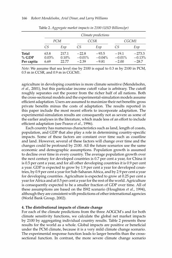
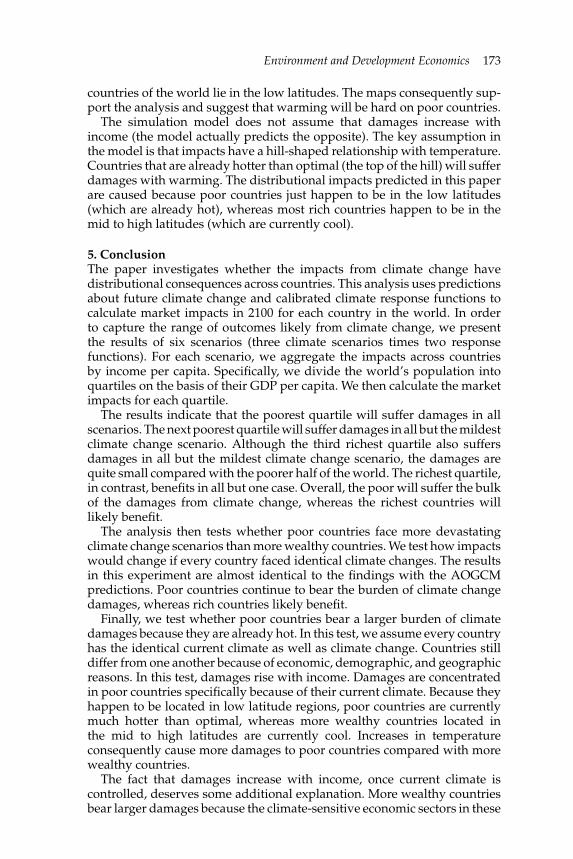
Figure 1. Generic hill-shaped impact response function

We want to make clear that this paper does not explain why some coun-tries are poor and others are rich. The standard neoclassical economicgrowth framework asserts that growth depends primarily on basic eco-nomic inputs such as trained labor, capital, and technological development(Solow, 1956). These basic economic factors have been extended to in-corporate government policies, the accumulation of human capital, fertilitydecisions, and the diffusion of technology (Barro, 1997; Bloom and Sachs,1999; Easterly and Devine, 1998; Barro and Sali-i-Martin, 2004). Our paperhas nothing to add to this important debate on growth.

The purpose of this paper is to examine whether there are importantdistributional consequences of climate change impacts. The early literatureon greenhouse gases did not raise serious concerns about the distributionalimpact of climate change (Nordhaus, 1991; Tol, 1995; Fankhauser, 1995;Pearce et al., 1996). This early literature largely assumed that damageswere a linear or quadratic function of the change in temperature. As aresult, the early models predicted that every country would suffer damagesfrom warming and that they would be roughly proportional to income.Developing countries were predicted to be slightly more vulnerable becauseso much of their economies were in climate-sensitive sectors such asagriculture and because low technology operations are expected to haveless substitution (Fankhauser, 1995; Tol, 1995). The literature at this time,however, assumed that almost every region would be damaged by warming(Pearce et al., 1996). Further, this sentiment extended to other chapters inthe Second Assessment Report of the IPCC where cross-country equity andcompensation to low-income countries was overlooked (Arrow et al., 1996;Jepma et al., 1996).

Subsequent empirical research on climate impact sensitivity has re-vealed new insights into how temperature affects climate-sensitive eco-nomic sectors (Mendelsohn and Neumann, 1999; McCarthy et al., 2001;Mendelsohn, 2001; Tol, 2002). The new research indicates that severalclimate-sensitive sectors have a hill-shaped relationship with absolutetemperature. Figure 1 illustrates this relationship in general. For each sector,

Environment and Development Economics 161

there is an optimum temperature that maximizes welfare in that sector. Forfarmers in regions that are cooler than the optimum temperature, warmingwould cause net revenues to go up. For farmers in regions that are warmerthan the optimum temperature, warming would cause net revenues tofall. These results imply that countries that happen to be in relatively coolregions of the world will likely benefit from warming and that countriesthat happen to be in relatively warm regions of the world will likely beharmed by warming.

We quantify the market impacts of climate change on every countryin the world by combining a range of future climate scenarios with arange of climate response functions and background information from eachcountry. The next section describes the country-specific climate forecastsfrom the three Atmospheric Ocean General Circulation Models (AOGCM’s)used in the paper (Houghton et al., 2001). Section 3 discusses the twosets of climate response functions used to evaluate the climate forecasts(Mendelsohn and Schlesinger, 1999). One set of response functions has ahigh and the other set a low climate sensitivity. Within each set, there is aseparate response function for each of the five major economic sectors thatare expected to be affected by climate: agriculture, water, energy, timber,and coasts1 (Smith and Tirpak, 1990; Pearce et al., 1996; Mendelsohn andNeumann, 1999; McCarthy et al., 2001). Using country-specific backgroundinformation on such variables as cropland, coastland, population, andGDP, we use previously calibrated response functions (Mendelsohn andSchlesinger, 1999) to develop quantitative forecasts of the impacts in eachsector for each country for each climate scenario (Mendelsohn et al., 2000a).We then sum these sectoral impacts to get an aggregate impact for eachcountry. These country-level market impacts are then summed to get multi-country/regional aggregate outcomes.

Non-market impacts to health, the environment, and aesthetics are notincluded in the calculations. Although non-market effects will certainlyadd to expected damages, reliable estimates of the magnitude of theresulting welfare impacts do not yet exist. The reported market impactsthus underestimate the total impacts of warming. However, it is likely thatthe non-market impacts will not change the distributional consequences ofwarming. Health effects and aesthetic effects are likely to strike low latitudecountries the hardest as well. Only ecological changes have an ambiguousdistributional outcome.

In section 4, we use these tools to evaluate the distributional impacts ofclimate change. First, the world’s population is divided into quartiles onthe basis of per capita income in 2100. The predicted impacts of the threeclimate models and two response functions are displayed for each quartile.The results indicate that the poorest half of the world’s nations suffer thebulk of the damages from climate change, whereas the wealthiest quarterhas almost no net impacts.

1 Technically, the early literature also assumed that there would be commercialfishery losses. They have not been included here because the ecological linkbetween warming and fishery losses is still speculative and so it is not knownhow fisheries would change. Further, fishery impacts are likely to be small sincethis is a small sector, but that may not be true for some countries.


There are many reasons why rich and poor countries are different andthey are all included in the results across quartiles. We consequently engagein two tests to isolate whether climate change and initial climate play animportant role. In order to test the role of climate change, we assume allcountries face identical climate change, although everything else about thecountries may differ. We do a similar test with respect to initial climateby assuming that every country has the identical initial climate. The testsreveal that forcing climate change to be the same has no effect on thedistributional outcome of impacts. The poor still bear the brunt of theworld’s damages. However, forcing the initial climate to be the same for allcountries changes the distributional results. If all countries had the sameinitial climate, the absolute magnitude of climate damages would rise withincome, because richer nations have larger climate-sensitive sectors. As afraction of GDP, poorer nations would still suffer higher climate damagesthan richer nations, but the difference is small. These tests reveal thatthe poor nations of the world bear the brunt of climate change damagesprimarily because they are located in the low latitudes and are already toohot. The rich nations may well benefit from climate change because they arelocated in the mid to high latitudes and are currently cool. The proportionof GDP in agriculture, technology, wealth, and adaptation contribute to thedistributional outcome, but play a smaller role. These strong distributionalresults across countries suggest that compensation needs to be a part of thegreenhouse gas policy agenda along with mitigation and adaptation. Thefinal section of the paper discusses some policy alternatives.

2. Climate scenariosWe explore the results of three AOGCM’s to predict the impact of green-house gases. The Parallel Climate Model (PCM) comes from the NationalCenter Atmospheric Research (Washington et al., 2000). The Center forClimate Research Studies (CCSR) model was developed at NIES (Emoriet al., 1999). The Canadian General Circulation Model (CGCM1) was de-veloped at the Canadian Climate Centre (Boer et al., 2000). All three modelsare dynamic coupled ocean–atmosphere models that include greenhousegases and sulfates. The PCM and CCSR models assume the IS92a path ofgreenhouse gases and the CGCM1 model assumes a 1 per cent exponentialpath of greenhouse gases. These two paths result in CO2 levels of 685ppmvfor PCM and CCSR and 808ppmv in CGCM1 by 2100.

These three models were selected to demonstrate the consequences of afull range of climate scenarios. Each model predicts changes in individualgrid points across the earth. We use the grid points in each country to createa climate change scenario by country for 2100. The grid points are weightedby population and not by area. We prefer the population weighting methodof evaluating climate change forecasts because most impacts occur nearwhere people are living (Williams et al., 1998; Mendelsohn et al., 2000b).The population-weighted changes for each country are the inputs to theimpact model. We also use population weights to generate regional averagechanges in temperature and precipitation.

The three models make very different forecasts of global temperaturechange: PCM predicts 2.5C, CCSR predicts 4.0C, and CGCM1 predicts 5.2C


Table 1. Changes in temperature and precipitation predicted by each climatemodel in 2100

PCM CCSR CGCM1

Region T(C◦) P(%) T(C◦) P(%) T(C◦) P(%)

L. Amer. 2.0 5.9 3.3 −10.8 4.9 −4.3Africa 2.3 11.9 3.9 11.6 6.2 −10.3S. Asia 2.4 21.5 3.6 16.1 4.5 −1.6Pacific 1.8 7.3 2.6 14.4 4.2 −8.6N. Amer. 2.4 7.9 5.5 −23.1 5.4 1.7Europe 2.4 8.2 5.3 −6.0 3.9 −1.8N. Asia 2.9 22.5 4.0 10.0 6.4 −12.6FSU 3.5 10.2 5.7 9.6 7.1 9.9Globe 2.5 15.5 4.0 7.7 5.2 −5.6

Note: Temperature changes measured in centigrade and precipitation inpercentage changes. The climate measurements are weighted by populationnot area.

by 2100. Global precipitation changes also vary by model. PCM predictsa 16 per cent increase, CCSR predicts an 8 per cent increase, and CGCM1predicts a 6 per cent decrease in global precipitation by 2100.

The distribution of population weighted temperature changes acrosscontinents varies as seen in table 1. Warming is expected to increase withlatitude (Houghton et al., 2001). PCM and CCSR follow this accepted patternand show more warming in the polar and temperate regions versus thetropical regions. CCSR predicts that this difference across latitudes will beextreme, whereas PCM shows more modest differences. CGCM1 shows amore random flux of temperatures, with Africa getting especially hot butWestern Europe warming less than the rest of the planet.

The AOGCM models also predict a wide range of changes in population-weighted precipitation. PCM predicts higher precipitation in every con-tinent, but especially in Africa, North Asia, and South Asia. CCSR predictslarge losses of precipitation in Latin America and North America and smalllosses in Europe but large gains elsewhere. CGCM1 predicts losses ofprecipitation in every continent except North America and North Asia.There is clearly no consensus across the models about what will happen tolocal precipitation. However, the models do suggest that local precipitationmight change significantly in very different ways across the planet.

The climate scenarios provide four driving forces that can have an effecton economic sectors: changes in mean or seasonal temperature, changes inmean or seasonal precipitation, increases in carbon dioxide, and increasesin sea level. In addition to these climate changes, global warming can alsocause an increase in the variance of temperature and precipitation, a slowingof the thermohaline circulation (resulting in northern cooling), and thesudden loss of ice sheets (rapid sea level rise). These latter forces were notevaluated in this paper, partially because they are more speculative andpartially because there is less known about their timing and magnitude.


3. Impact methodologyWe look at two different empirical approaches to determine the climatesensitivity of each economic sector: experimental and cross-sectionalstudies. The experimental studies have been done in controlled settingssuch as laboratories or greenhouses (see Reilly et al., 1996 for a goodsummary of experimental results in agriculture). These studies carefullycontrol for unwanted variables but they struggle to include adaptationfully. In contrast, cross-sectional studies examine actual outcomes fromplace to place in order to measure climate impacts. The Ricardian methodis a good example of this approach in agriculture where the values offarms in different climates are compared (Mendelsohn et al., 1994). Thecross-sectional studies include efficient adaptation by design, but theystruggle to control for unwanted influences. Comparing the experimentaland cross-sectional method, the strength of each empirical methodologyis the weakness of the other. The experimental method has the addedadvantage that it can measure the direct effect of carbon dioxide, whichthe cross-sectional method cannot.2 Both models predict that temperaturehas a hill-shaped relationship with agriculture, forestry, water, and energy;that increased precipitation is generally beneficial; and that coastal damagesincrease as sea level rises. Details about the shapes of these functions canbe found in Mendelsohn and Schlesinger (1999).

The results from experimental studies lead to steeper hill-shapedclimate response functions compared with the cross-sectional results. Theexperimental model predicts that countries that are cooler than optimumwill gain more from warming and countries that are warmer than optimumwill lose more than the cross-sectional model predicts. As in the cross-sectional model, precipitation is predicted to have a beneficial impact onagriculture, forestry, and water but no effect on energy. The experimentalmodel depends only on average annual climate, whereas the cross-sectionalmodel captures a full array of seasonal temperatures and precipitationlevels. Carbon dioxide, through fertilization, is strictly beneficial and helpsforestry and especially agriculture in all regions (see Reilly et al., 1996 andSohngen et al., 2002). It is assumed that carbon fertilization benefits increasewith the log of CO2 and are the same in both models.

In a complete general equilibrium model, global warming could changethe supply and demand of all goods and services, leading to new globalprices for everything. In practice, the climate changes expected over the nexthundred years will not change overall economic conditions enough to affectmost prices. For example, across a host of climate scenarios, market damagesas a fraction of GDP were estimated to be less than 1 per cent (Mendelsohnet al., 2000b). Even the higher estimates found in the early literature sug-gested that damages would be just 2 per cent of GDP (Pearce et al., 1996). Suchsmall changes in output do not warrant using a general equilibrium model.

Most price changes that will occur because of warming will be limitedto the sectors directly affected by climate change. In these sectors, warmingwould affect consumers and suppliers across the world through direct

2 Carbon dioxide effects from the experimental studies are used to predict carbondioxide impacts in the cross-sectional results.


effects and prices could change. Models that take these price effects intoaccount have been constructed to study climate impacts on timber (Sohngenet al., 2002). Reliable global models for agriculture and energy have notyet been developed.3 This paper relies on studies that assume climatehas no effect on output prices in agriculture, timber, and energy. Globalimpact studies of these sectors have not been done but it is likely thatclimate-induced global price changes would be small. However, if this isnot the case, assuming constant prices biases the welfare estimates. If climatechange causes global scarcity and therefore increases prices, the presentedresults will underestimate total damages and miss consumer damagescompletely. If climate change increases abundance and reduces prices,the presented results will overestimate total benefits and miss consumerbenefits completely. What will happen to supplier welfare is ambiguous.

In contrast to the sectors with global markets, water is likely to haveonly a regional market because it is hard to transfer across basins. Watersupply and demand in specific regions can change dramatically acrossclimate scenarios and so there could be profound local price effects. Theseare captured by the model, which measures basin water prices using watersupply and demand changes (Hurd et al., 1999).

Two response functions to sea level rise are used in the model (Neumannand Livesay, 2001). In the cross-section model, we assume that landownershave foresight and so they depreciate buildings, anticipating they will beabandoned to sea level rise. In the experimental model, we assume thatlandowners have no foresight and that leads to slightly higher costs. Thecoastal study examines a series of decisions made each decade to eitherprotect or abandon coastline in response to the rising seas. By stretchingout responses across the century, costs are held to a relatively low levelin each decade. At least in the US and Singapore, the model predictsthat valuable coastlines will be protected (Neumann and Livesay, 2001;Ng and Mendelsohn, 2005). However, coastal protection is an adaptiveresponse that generally requires government planning and coordination. Itis not clear whether governments will make efficient decisions to protectcoastlines.

We find that the hill-shaped response functions are slightly differentbetween developed and developing countries (Mendelsohn et al., 2001). Thedeveloping countries have lower crop net revenues per hectare and theyare more temperature sensitive. The agriculture crop response functions totemperature in both developed and developing countries are hill shaped.But the developed country response function is both higher and flatterthan the developing country response function, presumably because thehigh technology farmers have more capital and they can substitute capitalfor climate. The model predicts that agriculture in developing countriesis more vulnerable to higher than optimal temperatures. We assume thatthis more vulnerable climate response function applies to countries whose2100 per capita income is less than $7,000. Empirical research suggests that

3 There are some well-calibrated general equilibrium models in agriculture thatexamine country-specific impacts (see for example Adams et al., 1999), but thesesimply assume global price changes.


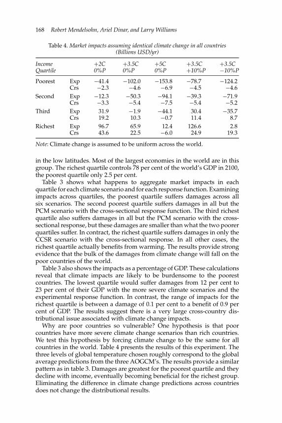
Table 2. Aggregate market impacts in 2100 (USD Billions/yr)

Climate predictions

PCM CCSR CGCM1

CS Exp CS Exp CS Exp

Total 63.8 217.1 −22.8 −93.5 −19.1 −273.3% GDP 0.03% 0.10% −0.01% −0.04% −0.01% −0.13%Per capita 6.69 22.77 −2.39 −9.81 −2.00 −28.7

Note: We assume that sea level rise by 2100 is equal to 0.3 m by 2100 in PCM,0.5 m in CCSR, and 0.9 m in CGCM1.

agriculture in developing countries is more climate sensitive (Mendelsohn,et al., 2001), but this particular income cutoff value is arbitrary. The cutoffroughly separates out the poorer from the richer half of all nations. Boththe cross-sectional models and the experimental-simulation models assumeefficient adaptation. Users are assumed to maximize their net benefits: grossprivate benefits minus the costs of adaptation. The results reported inthis paper include the most recent efforts to incorporate adaptation. Theexperimental-simulation results are consequently not as severe as some ofthe earlier analyses in the literature, which made less of an effort to includeefficient adaptation (see Pearce et al., 1996).

Each country has numerous characteristics such as land, length of coasts,population, and GDP that also play a role in determining country-specificimpacts. Some of these factors are constant over time such as coastlineand land. However, several of these factors will change over time and thechanges could be profound by 2100. All the future scenarios use the sameeconomic and demographic assumptions. Population growth is assumedto decline over time in every country. The average population growth overthe next century for developed countries is 0.7 per cent a year, for China itis 0.5 per cent a year, and for all other developing countries it is 0.9 per centa year. GDP is expected to grow by 1.9 per cent a year for developed coun-tries, by 0.9 per cent a year for Sub-Saharan Africa, and by 2.9 per cent a yearfor developing countries. Agriculture is expected to grow at 0.25 per cent ayear for Africa and at 0.5 per cent a year for the rest of the world. Agricultureis consequently expected to be a smaller fraction of GDP over time. All ofthese assumptions are based on the IS92 scenario (Houghton et al., 1994),although they are consistent with predictions of other international agencies(World Bank Group, 2002).

4. The distributional impacts of climate changeFor each of the climate predictions from the three AOGCM’s and for bothclimate sensitivity functions, we calculate the global net market impactsby 2100 by aggregating individual country results. Table 2 presents theseresults for the world as a whole. Global impacts are positive or beneficialunder the PCM climate, because it is a very mild climate change scenario.The experimental response function leads to larger benefits than the cross-sectional function. In contrast, the more severe climate change scenario


Table 3. Market impacts in 2100 by income (Billions USD/yr)

Impacts by climate predictions

PCM CCSR CGCM1

Income Cross Cross CrossGroup section Experimental section Experimental section Experimental

Poorest Impact −1.2 −8.0 −4.8 −69.4 −6.9 −140.7Quartile %GDP −0.2 −1.4 −0.8 −11.8 −1.2 −23.8Second Impact 4.5 19.7 −5.6 −30.2 −9.5 −92.0Quartile %GDP −0.4 1.6 −0.5 −2.4 −0.8 −7.4Third Impact 21.8 56.6 −0.7 −7.1 −4.5 −64.1Quartile %GDP 0.8 2.1 −0.0 −0.3 −0.2 −2.4Richest Impact 38.8 148.7 −11.7 13.2 1.8 23.5Quartile %GDP 0.2 0.9 −0.1 0.1 0.0 0.1

in CCSR is predicted to lead to small global net damages in both caseswith experimental results again being larger. Finally, under the severeclimate change scenario in CGCM1, damages will be slightly smaller forthe cross-sectional response function but much larger for the experimentalresponse function. This range of global net impacts is consistent with theThird Assessment Report of the IPCC, although the Report focuses moreon the potentially harmful end of this range (McCarthy et al., 2001). Annualmarket impacts as a fraction of GDP in 2100 range from slightly beneficial(+0.1 per cent of GDP) to slightly harmful (−0.12 per cent of GDP). Thesemarket impacts amount to an annual benefit of about $23 per person to aloss of about $27 per person.

It is clear that the different climate change scenarios have a large impacton the overall results one sees for the world. Specifically future climatescenarios that predict larger temperature increases and precipitation losses,lead to larger overall net global damages. However, the focus of this paperis upon the distributional impacts of these global changes, not their overallmagnitude.

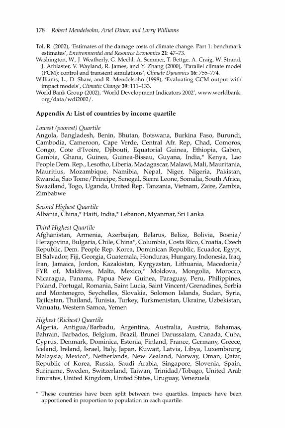
In order to understand how these climate impacts affect countries ofdifferent income levels, we order countries by per capita income in 2100.We then divide the country list into quartiles on the basis of their projectedpopulation in 2100. Each quartile represents one-fourth of the world’spopulation by 2100. A list of all countries and which quartile they fallin are shown in the Appendix. Table 3 shows the market impact resultsby quartile. The poorest quartile earns less than $4,380 per capita andincludes 53 countries, mostly from Africa. The second quartile group earnsfrom $4,380 to $5,785 per capita and includes only six countries, notablyIndia and China. The third quartile earns between $5,785 and $25,000and includes 65 countries from all over the world. Although the bulk ofthese countries are from warm latitudes, there are a few cooler countriesin this group. The richest quartile of the world’s population includes52 countries from North America, Europe, and the Middle East and ahandful of countries from other continents. The richest quartile includesmost of the countries in the mid–high latitudes and a scattering of countries


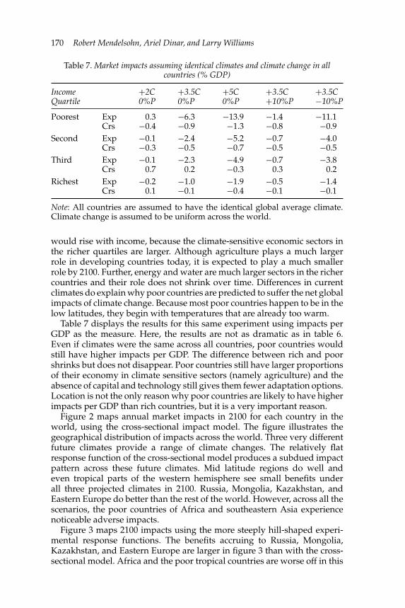
Table 4. Market impacts assuming identical climate change in all countries(Billions USD/yr)

Income +2C +3.5C +5C +3.5C +3.5CQuartile 0%P 0%P 0%P +10%P −10%P

Poorest Exp −41.4 −102.0 −153.8 −78.7 −124.2Crs −2.3 −4.6 −6.9 −4.5 −4.6

Second Exp −12.3 −50.3 −94.1 −39.3 −71.9Crs −3.3 −5.4 −7.5 −5.4 −5.2

Third Exp 31.9 −1.9 −44.1 30.4 −35.7Crs 19.2 10.3 −0.7 11.4 8.7

Richest Exp 96.7 65.9 12.4 126.6 2.8Crs 43.6 22.5 −6.0 24.9 19.3

Note: Climate change is assumed to be uniform across the world.

in the low latitudes. Most of the largest economies in the world are in thisgroup. The richest quartile controls 78 per cent of the world’s GDP in 2100,the poorest quartile only 2.5 per cent.

Table 3 shows what happens to aggregate market impacts in eachquartile for each climate scenario and for each response function. Examiningimpacts across quartiles, the poorest quartile suffers damages across allsix scenarios. The second poorest quartile suffers damages in all but thePCM scenario with the cross-sectional response function. The third richestquartile also suffers damages in all but the PCM scenario with the cross-sectional response, but these damages are smaller than what the two poorerquartiles suffer. In contract, the richest quartile suffers damages in only theCCSR scenario with the cross-sectional response. In all other cases, therichest quartile actually benefits from warming. The results provide strongevidence that the bulk of the damages from climate change will fall on thepoor countries of the world.

Table 3 also shows the impacts as a percentage of GDP. These calculationsreveal that climate impacts are likely to be burdensome to the poorestcountries. The lowest quartile would suffer damages from 12 per cent to23 per cent of their GDP with the more severe climate scenarios and theexperimental response function. In contrast, the range of impacts for therichest quartile is between a damage of 0.1 per cent to a benefit of 0.9 percent of GDP. The results suggest there is a very large cross-country dis-tributional issue associated with climate change impacts.

Why are poor countries so vulnerable? One hypothesis is that poorcountries have more severe climate change scenarios than rich countries.We test this hypothesis by forcing climate change to be the same for allcountries in the world. Table 4 presents the results of this experiment. Thethree levels of global temperature chosen roughly correspond to the globalaverage predictions from the three AOGCM’s. The results provide a similarpattern as in table 3. Damages are greatest for the poorest quartile and theydecline with income, eventually becoming beneficial for the richest group.Eliminating the difference in climate change predictions across countriesdoes not change the distributional results.


Table 5. Current observed temperature and precipitation in each region

Region Temperature (C) Precipitation

Africa 29.1 7.2South Asia 28.5 10.0Latin America 25.9 11.9Pacific 29.6 18.3North Asia 19.7 7.4North America 19.5 8.0Europe 13.7 6.1Former Soviet Union 12.0 4.8

Note: Observed measurements are population weighted averages not areaweighted averages as usually shown.

Table 6. Market impacts assuming identical climates and climate change in allcountries (Billions USD/yr)


Poorest Exp 1.8 −37.4 −82.0 −8.5 −65.3Crs −2.2 −5.0 −7.7 −5.0 −5.0

Second Exp −0.8 −29.7 −64.6 −9.2 −50.2Crs −3.4 −6.1 −8.8 −6.0 −5.9

Third Exp −2.1 −60.9 −131.7 −19.6 −102.3Crs 17.8 5.7 −8.6 7.0 4.6

Richest Exp −30.8 −156.2 −304.4 −80.0 −232.4Crs 21.9 −14.9 −59.3 −11.6 −17.0

Note: All countries are assumed to have the identical global average climate.Climate change is assumed to be uniform across the world.

An alternative hypothesis is that poor countries are more vulnerablebecause they are located in the low latitudes and have higher currentobserved temperatures. Table 5 shows the current variation in temperatureand precipitation by region. These starting climates can be very importantbecause they determine whether a sector is already too hot or too coolcompared with the optimum for that sector. Table 5 shows that the lowlatitude regions are currently hot. These temperatures are actually beyondthe optimum for most climate-sensitive economic sectors. In contrast,the mid latitude regions enjoy a range of current temperatures near theoptimum. The former Soviet Union and northern Europe have cool currenttemperatures that make warming good for their economy.

In tables 6 and 7, we assume that all countries have the same climateboth now and in the future. This assumption places every country underthe same climate experiment, although it allows countries to be different inother ways. As shown in table 6, if both present and future climates are thesame in every country, it would no longer be true that the poorest countrieswould suffer the brunt of the damages from climate change. In fact, damages


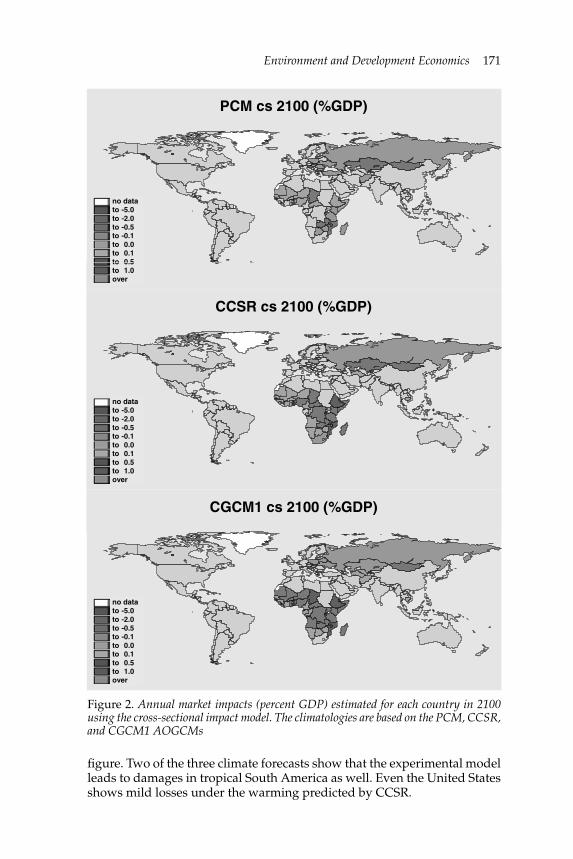
Table 7. Market impacts assuming identical climates and climate change in allcountries (% GDP)


Poorest Exp 0.3 −6.3 −13.9 −1.4 −11.1Crs −0.4 −0.9 −1.3 −0.8 −0.9

Second Exp −0.1 −2.4 −5.2 −0.7 −4.0Crs −0.3 −0.5 −0.7 −0.5 −0.5

Third Exp −0.1 −2.3 −4.9 −0.7 −3.8Crs 0.7 0.2 −0.3 0.3 0.2

Richest Exp −0.2 −1.0 −1.9 −0.5 −1.4Crs 0.1 −0.1 −0.4 −0.1 −0.1

Note: All countries are assumed to have the identical global average climate.Climate change is assumed to be uniform across the world.

would rise with income, because the climate-sensitive economic sectors inthe richer quartiles are larger. Although agriculture plays a much largerrole in developing countries today, it is expected to play a much smallerrole by 2100. Further, energy and water are much larger sectors in the richercountries and their role does not shrink over time. Differences in currentclimates do explain why poor countries are predicted to suffer the net globalimpacts of climate change. Because most poor countries happen to be in thelow latitudes, they begin with temperatures that are already too warm.

Table 7 displays the results for this same experiment using impacts perGDP as the measure. Here, the results are not as dramatic as in table 6.Even if climates were the same across all countries, poor countries wouldstill have higher impacts per GDP. The difference between rich and poorshrinks but does not disappear. Poor countries still have larger proportionsof their economy in climate sensitive sectors (namely agriculture) and theabsence of capital and technology still gives them fewer adaptation options.Location is not the only reason why poor countries are likely to have higherimpacts per GDP than rich countries, but it is a very important reason.

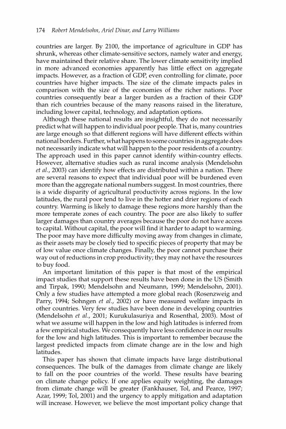
Figure 2 maps annual market impacts in 2100 for each country in theworld, using the cross-sectional impact model. The figure illustrates thegeographical distribution of impacts across the world. Three very differentfuture climates provide a range of climate changes. The relatively flatresponse function of the cross-sectional model produces a subdued impactpattern across these future climates. Mid latitude regions do well andeven tropical parts of the western hemisphere see small benefits underall three projected climates in 2100. Russia, Mongolia, Kazakhstan, andEastern Europe do better than the rest of the world. However, across all thescenarios, the poor countries of Africa and southeastern Asia experiencenoticeable adverse impacts.

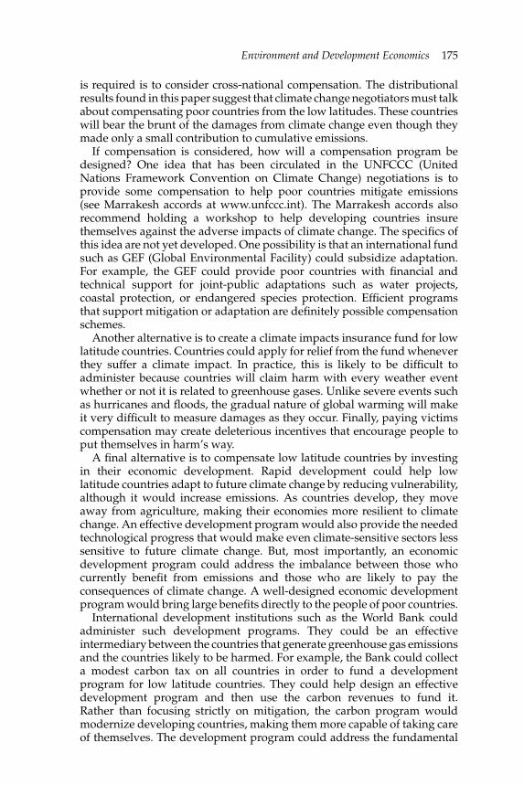
Figure 3 maps 2100 impacts using the more steeply hill-shaped experi-mental response functions. The benefits accruing to Russia, Mongolia,Kazakhstan, and Eastern Europe are larger in figure 3 than with the cross-sectional model. Africa and the poor tropical countries are worse off in this


PCM cs 2100 (%GDP)

no datato -5.0to -2.0to -0.5to -0.1to 0.0to 0.1to 0.5to 1.0over


CCSR cs 2100 (%GDP)



CGCM1 cs 2100 (%GDP)



Figure 2. Annual market impacts (percent GDP) estimated for each country in 2100using the cross-sectional impact model. The climatologies are based on the PCM, CCSR,and CGCM1 AOGCMs

figure. Two of the three climate forecasts show that the experimental modelleads to damages in tropical South America as well. Even the United Statesshows mild losses under the warming predicted by CCSR.


PCM exp 2100 (%GDP)



CCSR exp 2100 (%GDP)



CGCM1 exp 2100 (%GDP)



Figure 3. Annual market impacts (percent GDP) estimated for each country in 2100using the experimental impact model. The climatologies are based on the PCM, CCSR,and CGCM1 AOGCMs

The maps of figures 2 and 3 (color maps are available from the authorsupon request) reveal that under all climate forecasts and with both impactmodels, the poor countries of Africa and Southeast Asia are harmed byprojected climate change in 2100. These results demonstrate that the low lati-tude regions will be hard hit by climate change. Almost all of the poor


countries of the world lie in the low latitudes. The maps consequently sup-port the analysis and suggest that warming will be hard on poor countries.

The simulation model does not assume that damages increase withincome (the model actually predicts the opposite). The key assumption inthe model is that impacts have a hill-shaped relationship with temperature.Countries that are already hotter than optimal (the top of the hill) will sufferdamages with warming. The distributional impacts predicted in this paperare caused because poor countries just happen to be in the low latitudes(which are already hot), whereas most rich countries happen to be in themid to high latitudes (which are currently cool).

5. ConclusionThe paper investigates whether the impacts from climate change havedistributional consequences across countries. This analysis uses predictionsabout future climate change and calibrated climate response functions tocalculate market impacts in 2100 for each country in the world. In orderto capture the range of outcomes likely from climate change, we presentthe results of six scenarios (three climate scenarios times two responsefunctions). For each scenario, we aggregate the impacts across countriesby income per capita. Specifically, we divide the world’s population intoquartiles on the basis of their GDP per capita. We then calculate the marketimpacts for each quartile.

The results indicate that the poorest quartile will suffer damages in allscenarios. The next poorest quartile will suffer damages in all but the mildestclimate change scenario. Although the third richest quartile also suffersdamages in all but the mildest climate change scenario, the damages arequite small compared with the poorer half of the world. The richest quartile,in contrast, benefits in all but one case. Overall, the poor will suffer the bulkof the damages from climate change, whereas the richest countries willlikely benefit.

The analysis then tests whether poor countries face more devastatingclimate change scenarios than more wealthy countries. We test how impactswould change if every country faced identical climate changes. The resultsin this experiment are almost identical to the findings with the AOGCMpredictions. Poor countries continue to bear the burden of climate changedamages, whereas rich countries likely benefit.

Finally, we test whether poor countries bear a larger burden of climatedamages because they are already hot. In this test, we assume every countryhas the identical current climate as well as climate change. Countries stilldiffer from one another because of economic, demographic, and geographicreasons. In this test, damages rise with income. Damages are concentratedin poor countries specifically because of their current climate. Because theyhappen to be located in low latitude regions, poor countries are currentlymuch hotter than optimal, whereas more wealthy countries located inthe mid to high latitudes are currently cool. Increases in temperatureconsequently cause more damages to poor countries compared with morewealthy countries.

The fact that damages increase with income, once current climate iscontrolled, deserves some additional explanation. More wealthy countriesbear larger damages because the climate-sensitive economic sectors in these


countries are larger. By 2100, the importance of agriculture in GDP hasshrunk, whereas other climate-sensitive sectors, namely water and energy,have maintained their relative share. The lower climate sensitivity impliedin more advanced economies apparently has little effect on aggregateimpacts. However, as a fraction of GDP, even controlling for climate, poorcountries have higher impacts. The size of the climate impacts pales incomparison with the size of the economies of the richer nations. Poorcountries consequently bear a larger burden as a fraction of their GDPthan rich countries because of the many reasons raised in the literature,including lower capital, technology, and adaptation options.

Although these national results are insightful, they do not necessarilypredict what will happen to individual poor people. That is, many countriesare large enough so that different regions will have different effects withinnational borders. Further, what happens to some countries in aggregate doesnot necessarily indicate what will happen to the poor residents of a country.The approach used in this paper cannot identify within-country effects.However, alternative studies such as rural income analysis (Mendelsohnet al., 2003) can identify how effects are distributed within a nation. Thereare several reasons to expect that individual poor will be burdened evenmore than the aggregate national numbers suggest. In most countries, thereis a wide disparity of agricultural productivity across regions. In the lowlatitudes, the rural poor tend to live in the hotter and drier regions of eachcountry. Warming is likely to damage these regions more harshly than themore temperate zones of each country. The poor are also likely to sufferlarger damages than country averages because the poor do not have accessto capital. Without capital, the poor will find it harder to adapt to warming.The poor may have more difficulty moving away from changes in climate,as their assets may be closely tied to specific pieces of property that may beof low value once climate changes. Finally, the poor cannot purchase theirway out of reductions in crop productivity; they may not have the resourcesto buy food.

An important limitation of this paper is that most of the empiricalimpact studies that support these results have been done in the US (Smithand Tirpak, 1990; Mendelsohn and Neumann, 1999; Mendelsohn, 2001).Only a few studies have attempted a more global reach (Rosenzweig andParry, 1994; Sohngen et al., 2002) or have measured welfare impacts inother countries. Very few studies have been done in developing countries(Mendelsohn et al., 2001; Kurukulasuriya and Rosenthal, 2003). Most ofwhat we assume will happen in the low and high latitudes is inferred froma few empirical studies. We consequently have less confidence in our resultsfor the low and high latitudes. This is important to remember because thelargest predicted impacts from climate change are in the low and highlatitudes.

This paper has shown that climate impacts have large distributionalconsequences. The bulk of the damages from climate change are likelyto fall on the poor countries of the world. These results have bearingon climate change policy. If one applies equity weighting, the damagesfrom climate change will be greater (Fankhauser, Tol, and Pearce, 1997;Azar, 1999; Tol, 2001) and the urgency to apply mitigation and adaptationwill increase. However, we believe the most important policy change that


is required is to consider cross-national compensation. The distributionalresults found in this paper suggest that climate change negotiators must talkabout compensating poor countries from the low latitudes. These countrieswill bear the brunt of the damages from climate change even though theymade only a small contribution to cumulative emissions.

If compensation is considered, how will a compensation program bedesigned? One idea that has been circulated in the UNFCCC (UnitedNations Framework Convention on Climate Change) negotiations is toprovide some compensation to help poor countries mitigate emissions(see Marrakesh accords at www.unfccc.int). The Marrakesh accords alsorecommend holding a workshop to help developing countries insurethemselves against the adverse impacts of climate change. The specifics ofthis idea are not yet developed. One possibility is that an international fundsuch as GEF (Global Environmental Facility) could subsidize adaptation.For example, the GEF could provide poor countries with financial andtechnical support for joint-public adaptations such as water projects,coastal protection, or endangered species protection. Efficient programsthat support mitigation or adaptation are definitely possible compensationschemes.

Another alternative is to create a climate impacts insurance fund for lowlatitude countries. Countries could apply for relief from the fund wheneverthey suffer a climate impact. In practice, this is likely to be difficult toadminister because countries will claim harm with every weather eventwhether or not it is related to greenhouse gases. Unlike severe events suchas hurricanes and floods, the gradual nature of global warming will makeit very difficult to measure damages as they occur. Finally, paying victimscompensation may create deleterious incentives that encourage people toput themselves in harm’s way.

A final alternative is to compensate low latitude countries by investingin their economic development. Rapid development could help lowlatitude countries adapt to future climate change by reducing vulnerability,although it would increase emissions. As countries develop, they moveaway from agriculture, making their economies more resilient to climatechange. An effective development program would also provide the neededtechnological progress that would make even climate-sensitive sectors lesssensitive to future climate change. But, most importantly, an economicdevelopment program could address the imbalance between those whocurrently benefit from emissions and those who are likely to pay theconsequences of climate change. A well-designed economic developmentprogram would bring large benefits directly to the people of poor countries.

International development institutions such as the World Bank couldadminister such development programs. They could be an effectiveintermediary between the countries that generate greenhouse gas emissionsand the countries likely to be harmed. For example, the Bank could collecta modest carbon tax on all countries in order to fund a developmentprogram for low latitude countries. They could help design an effectivedevelopment program and then use the carbon revenues to fund it.Rather than focusing strictly on mitigation, the carbon program wouldmodernize developing countries, making them more capable of taking careof themselves. The development program could address the fundamental


inequity of greenhouse gases and provide the poor nations of the worldwith immediate benefits.

ReferencesAdams, R., B. McCarl, K. Segerson, C. Rosenzweig, K. Bryant, B. Dixon, R. Conner,

R. Evenson, and D. Ojima (1999), ‘The economic effect of climate change on USagriculture’, in R. Mendelsohn and J. Neumann (eds), The Economic Impact ofClimate Change on the United States Economy, Cambridge: Cambridge UniversityPress.

Arrow, K., W. Cline, K.-G. Maler, M. Munasinghe, R. Squitteri, and J.E. Stiglitz. (1996),‘Intertemporal equity, discounting, and economic efficiency’, in J. Bruce, H. Lee,and E. Haites (eds), Climate Change 1995: Economic and Social Dimensions of ClimateChange, Cambridge: Cambridge University Press, pp. 125–144.

Azar, C. (1999), ‘Weight factors in cost-benefit analysis of climate change’,Environmental and Resource Economics 13: 249–268.

Barro, R.J. (1997), Determinants of Economic Growth, Cambridge, MA: MIT Press.Barro, R.J. and X. Sala-i-Martin (2004), Economic Growth, 2nd edn, Cambridge, MA:

MIT Press.Bloom, D. and J. Sachs (1999), ‘Geography, demography, and economic growth in

Africa’, Brookings Papers on Economic Activity 1998 2: 207–273.Boer, G., G. Flato, and D. Ramsden (2000), ‘A transient climate change simulation

with greenhouse gas and aerosol forcing: projected climate for the 21st century’,Climate Dynamics 16: 427–450.

Easterly, W. and R. Devine (1998), ‘Africa’s growth tragedy: policies and ethnicdivisions’, Quarterly Journal of Economics 112: 1203–1250.

Emori, S., T. Nozawa, A. Abe-Ouchi, A. Namaguti, and M. Kimoto (1999), ‘Coupledocean-atmospheric model experiments of future climate change with an explicitrepresentation of sulphate aerosol scattering’, Journal Meteorological Society Japan77: 1299–1307.

Fankhauser, S. (1995), Valuing Climate Change: The Economics of the Greenhouse,London: Earthscan.

Fankhauser, S., R.S.J. Tol, and D.W. Pearce (1997), ‘The aggregation of climate changedamages: a welfare theoretic approach’, Environmental and Resource Economics 10:249–266.

Houghton, J. T., L.G. Meira Filho, J. Bruce, H. Lee, B.A. Callander, E. Haites, N.Harris, and K. Maskell (eds) (1994), Climate Change 1994: Radiative Forcing ofClimate Change and an Evaluation of the IPCC IS92 Emission Scenarios, Cambridge:Cambridge University Press, 339 pp.

Houghton, J., Y. Ding, D. Griggs, M. Noguer, P. van der Linden, X. Dai, K. Maskell,and C. Johnson (eds) (2001), Climate Change 2001: The Scientific Basis. ThirdAssessment Report of the Intergovernmental Panel on Climate Change, Cambridge:Cambridge University Press.

Hurd, B., M. Callaway, J. Smith, and P. Kirshen (1999), ‘Economic effects of climatechange on US water resources’, in R. Mendelsohn and J. Neumann (eds), TheEconomic Impact of Climate Change on the United States Economy, Cambridge:Cambridge University Press.

Jepma, C. et al. (1996), ‘A generic assessment of response options’, in J. Bruce,H. Lee, and E. Haites (eds), Climate Change 1995: Economic and Social Dimensions ofClimate Change, Cambridge: Cambridge University Press, pp. 225–262.

Kurukurasuriya, P. and S. Rosenthal (2003), Climate Change and Agriculture: AReview of Impacts and Adaptations, Climate Change Series, 91, Agriculture andRural Development Department and Environment Department Joint Publication,Washington DC: The World Bank.

McCarthy, J., O. Canziani, N. Leary, D. Dokken, and K. White (eds) (2001), ClimateChange 2001: Impacts, Adaptation, and Vulnerability. Third Assessment Report of the


Intergovernmental Panel on Climate Change, Cambridge: Cambridge UniversityPress.

Mendelsohn, R. (ed.) (2001), Global Warming and the American Economy: A RegionalAnalysis, Camberley, Surrey: Edward Elgar Publishing.

Mendelsohn, R., A. Dinar, and A. Sanghi (2001), ‘The effect of development onthe climate sensitivity of agriculture’, Environment and Development Economics 6:85–101.

Mendelsohn, R., W. Morrison, M. Schlesinger, and N. Adronova (2000a), ‘Country-specific market impacts from climate change’, Climatic Change 45: 553–569.

Mendelsohn, R. and J. Neumann (eds) (1999), The Impact of Climate Change on theUnited States Economy, Cambridge: Cambridge University Press.

Mendelsohn, R., W. Nordhaus, and D. Shaw (1994), ‘Measuring the impact of globalwarming on agriculture’, American Economic Review 84: 753–771.

Mendelsohn, R. and M. Schlesinger (1999), ‘Climate response functions’, Ambio 28:362–366.

Mendelsohn, R., M. Schlesinger, and L. Williams (2000b), ‘Comparing impacts acrossclimate models’, Integrated Assessment 1: 37–48.

Mendelsohn, R. and L. Williams (2001), ‘Assessing the market damages from climatechange’, in J. Griffin (ed.), Global Climate Change: The Science, Economics, and Politics,Camberley, Surrey: Edward Elgar Publishing, pp. 92–113.

Neumann, J. and N. Livesay (2001), ‘Coastal structures: dynamic economicmodeling’, in R. Mendelsohn (ed.), Global Warming and the American Economy:A Regional Analysis, Camberley, Surrey: Edward Elgar Publishing, pp. 132–148.

Ng, W. and R. Mendelsohn (2005), ‘The impact of sea-level rise on Singapore’,Environment and Development Economics 10: 201–215.

Nordhaus, W. (1991), ‘To slow or not to slow: the economics of the greenhouse effect’,The Economic Journal 101: 920–937.

Pearce, D., W. Cline, A. Achanta, S. Fankhauser, R. Pachauri, R. Tol, and P. Vellinga.(1996), ‘The social cost of climate change: greenhouse damage and the benefitsof control’, in J. Bruce, H. Lee, and E. Haites (eds), Climate Change 1995: Economicand Social Dimensions of Climate Change, Cambridge: Cambridge University Press,pp. 179–224.

Pearce, D. (2003), ‘The social cost of carbon and its policy implications’, Oxford Reviewof Economic Policy 19: 362–384.

Reilly, J. et al. (1996), ‘Agriculture in a changing climate: Impacts and adaptations’,in IPCC (Intergovernmental Panel on Climate Change), R. Watson, M. Zinyowera,R. Moss, and D. Dokken (eds), Climate Change 1995. Impacts, Adaptations, andMitigation of Climate Change: Scientific-Technical Analyses, Cambridge: CambridgeUniversity Press, pp. 427–468.

Rosenzweig, C. and M. Parry (1994), ‘Potential impact of climate change on worldfood supply’, Nature 367: 133–138.

Schelling, T. (1992), ‘Some economics of global warming’, American Economic Review82: 1–14.

Smith, J. and D. Tirpak (1990), The Potential Effects of Global Climate Change on theUnited States: Report to Congress, US, Washington DC: Environmental ProtectionAgency.

Sohngen, B., R. Mendelsohn, and R. Sedjo (2002), ‘A global model of climate changeimpacts on timber markets’, Journal of Agricultural and Resource Economics 26: 326–343.

Solow, R. (1956), ‘A contribution to the theory of economic growth’, Quarterly Journalof Economics 70: 65–94.

Tol, R. (1995), ‘The damage costs of climate change: towards more comprehensiveestimates’, Environmental and Resource Economics 5: 353–374.

Tol, R. (2001), ‘Equitable cost–benefit analysis of climate change policies’, EcologicalEconomics 36: 71–85.


Tol, R. (2002), ‘Estimates of the damage costs of climate change. Part 1: benchmarkestimates’, Environmental and Resource Economics 21: 47–73.

Washington, W., J. Weatherly, G. Meehl, A. Semmer, T. Bettge, A. Craig, W. Strand,J. Arblaster, V. Wayland, R. James, and Y. Zhang (2000), ‘Parallel climate model(PCM): control and transient simulations’, Climate Dynamics 16: 755–774.

Williams, L., D. Shaw, and R. Mendelsohn (1998), ‘Evaluating GCM output withimpact models’, Climatic Change 39: 111–133.

World Bank Group (2002), ‘World Development Indicators 2002’, www.worldbank.org/data/wdi2002/.

Appendix A: List of countries by income quartile

Lowest (poorest) QuartileAngola, Bangladesh, Benin, Bhutan, Botswana, Burkina Faso, Burundi,Cambodia, Cameroon, Cape Verde, Central Afr. Rep, Chad, Comoros,Congo, Cote d’Ivoire, Djibouti, Equatorial Guinea, Ethiopia, Gabon,Gambia, Ghana, Guinea, Guinea-Bissau, Guyana, India,* Kenya, LaoPeople Dem. Rep., Lesotho, Liberia, Madagascar, Malawi, Mali, Mauritania,Mauritius, Mozambique, Namibia, Nepal, Niger, Nigeria, Pakistan,Rwanda, Sao Tome/Principe, Senegal, Sierra Leone, Somalia, South Africa,Swaziland, Togo, Uganda, United Rep. Tanzania, Vietnam, Zaire, Zambia,Zimbabwe

Second Highest QuartileAlbania, China,* Haiti, India,* Lebanon, Myanmar, Sri Lanka

Third Highest QuartileAfghanistan, Armenia, Azerbaijan, Belarus, Belize, Bolivia, Bosnia/Herzgovina, Bulgaria, Chile, China*, Columbia, Costa Rico, Croatia, CzechRepublic, Dem. People Rep. Korea, Dominican Republic, Ecuador, Egypt,El Salvador, Fiji, Georgia, Guatemala, Honduras, Hungary, Indonesia, Iraq,Iran, Jamaica, Jordon, Kazakistan, Kyrgyzstan, Lithuania, Macedonia/FYR of, Maldives, Malta, Mexico,* Moldova, Mongolia, Morocco,Nicaragua, Panama, Papua New Guinea, Paraguay, Peru, Philippines,Poland, Portugal, Romania, Saint Lucia, Saint Vincent/Grenadines, Serbiaand Montenegro, Seychelles, Slovakia, Solomon Islands, Sudan, Syria,Tajikistan, Thailand, Tunisia, Turkey, Turkmenistan, Ukraine, Uzbekistan,Vanuatu, Western Samoa, Yemen

Highest (Richest) QuartileAlgeria, Antigua/Barbadu, Argentina, Australia, Austria, Bahamas,Bahrain, Barbados, Belgium, Brazil, Brunei Darussalam, Canada, Cuba,Cyprus, Denmark, Dominica, Estonia, Finland, France, Germany, Greece,Iceland, Ireland, Israel, Italy, Japan, Kuwait, Latvia, Libya, Luxembourg,Malaysia, Mexico*, Netherlands, New Zealand, Norway, Oman, Qatar,Republic of Korea, Russia, Saudi Arabia, Singapore, Slovenia, Spain,Suriname, Sweden, Switzerland, Taiwan, Trinidad/Tobago, United ArabEmirates, United Kingdom, United States, Uruguay, Venezuela

* These countries have been split between two quartiles. Impacts have beenapportioned in proportion to population in each quartile.

Documents

The distributional impact of climate change on rich …nersp.osg.ufl.edu/~vecy/LitSurvey/Mendelsohn.06.pdfThe distributional impact of climate change on rich and poor countries ROBERT