Embed Size (px)
Citation preview
DOT/FAA/AR-9 7/7
Office of Aviation Research Washington, D.C. 20591
Advanced Pavement Design: Finite Element Modeling for Rigid Pavement Joints, Report II: Model Development
March 1998
Final Report
This document is available to the U.S. public through the National Technical Information Service (NTIS), Springfield, Virginia 22161.
U.S. Department of Transportation Federal Aviation Administr ation

NOTICE
This document is disseminated under the sponsorship of the U.S. Department of Transportation in the interest of information exchange. The United States Government assumes no liability for the contents or use thereof. The United States Government does not endorse products or manufacturers. Trade or manufacturer's names appear herein solely because they are considered essential to the objective of this report.

��������� ������ ������������� ����
�� ������ ���
DOT/FAA/AR-97/7
�� ���������� ��������� ��� �� ����������� ������� ���
�� ����� ��� ��������
ADVANCED PAVEMENT DESIGN: FINITE ELEMENT MODELING FOR RIGID PAVEMENT JOINTS, REPORT II: MODEL DEVELOPMENT
�� ������ ����
March 1998
�� ���������� ������������ ����
�� ���������
Michael I. Hammons
�� ���������� ������������ ������ ���
�� ���������� ������������ ���� ��� �������
U.S. Army Engineer Waterways Experiment Station 3909 Halls Ferry Road Vicksburg, MS 39180-6199
��� ���� ���� ��� �������
��� �������� �� ����� ���
DTFA03-94-X-00010
��� ���������� ������ ���� ��� �������
U.S. Department of Transportation Federal Aviation Administration Office of Aviation Research Washington, DC 20591
��� ���� �� ������ ��� ������ �������
Final Report
��� ���������� ������ ����
AAR-410
��� ������������� �����
FAA William J. Hughes Technical Center COTR is Xioagong Lee
��� ��������
The contribution of a cement-stabilized base course to the strength of the rigid pavement structure is poorly understood. The objective of this research was to obtain data on the response of the rigid pavement slab-joint-foundation system by conducting laboratory-scale experiments on jointed rigid pavement models and to develop a comprehensive three-dimensional (3D) finite element model of the rigid pavement slab-joint-foundation system that can be implemented in the advanced pavement design concepts currently under development by the Federal Aviation Administration. Evidence from experiments conducted on six laboratory-scale jointed rigid pavement models suggests that the joint effic iency depends upon the presence and condition of a stabilized base. The presence of cracking in the base and the degree of bonding between the slabs and the stabilized base course influence the structural capacity and load transfer capability of the rigid pavement structure. The finite element model developed in this research indicates that a comprehensive 3D finite element modeling technique provides a rational approach to modeling the structural response of the jointed rigid airport pavement system. Modeling features which are required include explicit 3D modeling of the slab continua, load transfer capability at the joint (modeled springs between the slabs), explicit 3D modeling of the base course continua, aggregate interlock capability across the cracks in the base course (again, modeled by springs across the crack), and contact interaction between the slabs and base course. The contact interaction model feature must allow gaps to open between the slab and base. Furthermore, where the slabs and base are in contact, transfer of shear stresses across the interface via friction should be modeled.
��� ��� �����
Aggregate interlock Finite elements Rigid pavements Contact Friction Stabilized bases Dowels Joints
��� ������������ ���������
This document is available to the public through the National Technical Information Service (NTIS), Springfield, VA 22161.
��� �������� �������� ��� ���� �������
Unclassified
��� �������� �������� ��� ���� �����
Unclassified
��� ��� �� �����
180
��� �����
���� ��� � ������ ������������ �� ��������� ���� ����������

PREFACE
The research reported herein was sponsored by the U.S. Department of Transportation, Federal Aviation Administration (FAA), Airport Technology Branch under Interagency Agreement DTFA03-94-X-00010 by the Airfields and Pavements Division (APD), Geotechnical Laboratory (GL), U.S. Army Engineer Waterways Experiment Station (WES), Vicksburg, Mississippi. Dr. Xiaogong Lee, Airport Technology Branch, FAA, was the technical monitor. Dr. Satish Agrawal is Manager, Airport Technology Branch, FAA.
This study was conducted under the general supervision of Dr. W. F. Marcuson III, Director, GL, and Dr. Raymond S. Rollings, Acting Chief, APD. This report was prepared under the direct supervision of Mr. T. W. Vollor, Chief, Materials Analysis Branch (MAB), APD. The project principal investigator was Mr. Michael I. Hammons, MAB. This report was written by Mr. Hammons. The assistance of Dr. Don Banks, Acting Assistant Director, GL, is gratefully acknowledged.
The Director of WES during the preparation of this publication was Dr. Robert W. Whalin. The Commander and Deputy Director was Colonel Bruce K. Howard, EN.
iii/iv

CONTENTS
Page
EXECUTIVE SUMMARY
1 INTRODUCTION
1.1 Background1.2 Objective1.3 Scope
2 FINITE ELEMENT CODE DESCRIPTION
2.1 Background2.2 Isoparametric Element Considerations2.3 Element Descriptions
2.3.1 2D Element Descriptions2.3.2 3D Element Descriptions
xv
1-1
1-1 1-3 1-4
2-1
2-1 2-1 2-5
2-5 2-8
3 SINGLE-SLAB RESPONSE AND SENSITIVITY STUDIES 3-1
3.1 Background3.2 Example Problems for Sensitivity Studies
3.2.1 Interior Load Case I3.2.2 Interior Load Case II3.2.3 Interior Load Case III3.2.4 Edge Load Case I3.2.5 Edge Load Case II
3.3 Response and Sensitivity Study Results
3.3.1 Interior Load Case I3.3.2 Interior Load Case II3.3.3 Interior Load Case III3.3.4 Edge Load Case I3.3.5 Edge Load Case II
4 JOINTED SLABS-ON-GRADE MODEL
4.1 Background4.2 Representation of Joint Stiffness4.3 Example Problem
3-1 3-1
3-2 3-2 3-4 3-5 3-7
3-7
3-8 3-15 3-16 3-18 3-21
4-1
4-1 4-2 4-7
v

5 CONTACT AND FRICTION MODELING 5-1
5.1 Problem Statement 5-15.2 Contact and Friction Options in ABAQUS 5-15.3 Simple Example Problem 5-2
6 SUMMARY OF RESPONSE AND SENSITIVITY STUDIES 6-1
7 EXPERIMENTS ON LABORATORY-SCALE PAVEMENT MODELS 7-1
7.1 Introduction7.2 Experimental Plan7.3 Materials
7.3.1 Concrete Materials7.3.2 Cement-Stabilized Base Materials7.3.3 Unbond Granular Base Material7.3.4 Dowels
7.4 Model Construction
7.4.1 Base Course Construction7.4.2 Slab Construction
7.5 Loading7.6 Instrumentation7.7 Experimental Results7.8 Materials
7.8.1 Cement-Stabilized Bases7.8.2 Portland Cement Concrete7.8.3 Rubber Block
7.9 Experiment LSM-1
7.9.1 Experiment LSM-1A7.9.2 Experiment LSM-1B7.9.3 Summary
7.10 Experiment LSM-27.11 Experiment LSM-3R7.12 Experiment LSM-47.13 Experiment LSM-57.14 Experiment LSM-67.15 Comparison of Experimental Results
7-1 7-1 7-4
7-4 7-5 7-8 7-8
7-9
7-11 7-13
7-14 7-15 7-16 7-16
7-16 7-17 7-20
7-23
7-24 7-29 7-33
7-33 7-36 7-39 7-42 7-45 7-48
vi

8 ANAL YTICAL MODEL DEVELOPMENT AND VERIFICATION 8-1
8.1 Analytical Model Description 8-1 8.2 Analytical Model Results 8-3
8.2.1 Case I 8-38.2.2 Case II 8-78.2.3 Case III 8-108.2.4 Case IV 8-138.2.5 Case V 8-17
8.3 Slab/Base Interaction and Joint Response 8-19
9 CONCLUSIONS AND RECOMMENDATIONS 9-1
9.1 Conclusions 9-19.2 Recommendations 9-2
10 REFERENCES 10-1
APPENDICES
AAlgorithm for Assigning Spring Stiffnesses to Nodes Using the Abaqus “JOINTC” Option
BCompilation of Instrumentation Traces From Experiments
vii
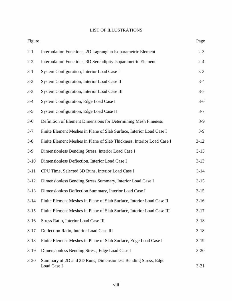
LIST OF ILLU STRATIONS
Figure Page
2-1 Interpolation Functions, 2D Lagrangian Isoparametric Element 2-3
2-2 Interpolation Functions, 3D Serendipity Isoparametric Element 2-4
3-1 System Configuration, Interior Load Case I 3-3
3-2 System Configuration, Interior Load Case II 3-4
3-3 System Configuration, Interior Load Case III 3-5
3-4 System Configuration, Edge Load Case I 3-6
3-5 System Configuration, Edge Load Case II 3-7
3-6 Definition of Element Dimensions for Determining Mesh Fineness 3-9
3-7 Finite Element Meshes in Plane of Slab Surface, Interior Load Case I 3-9
3-8 Finite Element Meshes in Plane of Slab Thickness, Interior Load Case I 3-12
3-9 Dimensionless Bending Stress, Interior Load Case I 3-13
3-10 Dimensionless Deflection, Interior Load Case I 3-13
3-11 CPU Time, Selected 3D Runs, Interior Load Case I 3-14
3-12 Dimensionless Bending Stress Summary, Interior Load Case I 3-15
3-13 Dimensionless Deflection Summary, Interior Load Case I 3-15
3-14 Finite Element Meshes in Plane of Slab Surface, Interior Load Case II 3-16
3-15 Finite Element Meshes in Plane of Slab Surface, Interior Load Case III 3-17
3-16 Stress Ratio, Interior Load Case III 3-18
3-17 Deflection Ratio, Interior Load Case III 3-18
3-18 Finite Element Meshes in Plane of Slab Surface, Edge Load Case I 3-19
3-19 Dimensionless Bending Stress, Edge Load Case I 3-20
3-20 Summary of 2D and 3D Runs, Dimensionless Bending Stress, EdgeLoad Case I 3-21
viii
3-21 Finite Element Meshes in Plane of Slab Surface, Edge Load Case II 3-22
3-22 Dimensionless Bending Stress, Default Transverse Shear Stiffness, EdgeLoad Case II 3-23
3-23 Dimensionless Bending Stress, 100 Times Default Transverse Shear Stiffness,Edge Load Case II 3-24
3-24 Dimensionless Deflection, Default Transverse Shear Stiffness, EdgeLoad Case II 3-24
3-25 Dimensionless Deflection, 100 Times Default Transverse Shear Stiffness,Edge Load Case II 3-25
3-26 Effect of Slab Width to Depth Ratio on Edge Stresses 3-26
3-27 Finite Element Distribution of τxzh2/p Through Slab Thickness 3-26
3-28 Theoretical and Experimental Dimensionless Bending Stress From Small-Scale Model Studies 3-27
3-29 Ratio of Theoretical to Experimental Bending Stress FromSmall-Scale Model Studies 3-28
4-1 Simply-Supported Beam Problem to Test JOINTC Element 4-6
4-2 Results From Simply-Supported Beam With JOINTC Element 4-7
4-3 Finite Element Mesh for 2D Jointed Rigid Pavement Model 4-9
4-4 Bending Stresses Predicted by 2D Finite Element Model of a JointedPavement 4-10
4-5 Comparison of Joint Response Parameters, 2D Finite Element Model 4-11
4-6 Comparison of Bending Stresses Predicted by 2D and 3D Finite ElementModels of a Jointed Pavement 4-12
4-7 Comparison of 3D Finite Element Model With Closed-Form Solution,Dimensionless Joint Stiffness Versus Deflection Load Transfer Efficiency 4-13
4-8 Comparison of 3D Finite Element Model With Closed-Form Solution, StressLoad Transfer Efficiency Versus Deflection Load Transfer Efficiency 4-13
5-1 Example of Overconstraint for Contact Problem 5-2
5-2 Simply-Supported Beam Problem to Test Contact Interaction Featuresof ABAQUS 5-2
ix

5-3 Results From Simply-Supported Beam With Contact and Friction 5-3
7-1 Experimental Configurations 7-3
7-2 Grain Size Distribution of Sand/Silica Flour Blend 7-6
7-3 Moisture-Density Curves for Cement-Stabilized Sand/Silica Flour Blend 7-7
7-4 Compressive Strength Test Results on Cement-Stabilized Sand/SilicaFlour Blend Compacted to Maximum Density 7-8
7-5 Dowel Locations 7-9
7-6 Photograph of Completed Reaction Box 7-10
7-7 Photograph of Adjustable Screed/Compaction Device 7-11
7-8 Installation of Polyethylene Film in Reaction Box 7-12
7-9 Placement of Thin Sand Layer 7-13
7-10 Bond Breaker and Doweled Joint Just Prior to Concrete Placement 7-13
7-11 Test Setup for Plate Bearing Test on Rubber Pad 7-21
7-12 Plate Bearing Stress-Displacement Data From Plate Bearing Test on RubberBlock in Load Control 7-22
7-13 Corrected Plate Bearing Stress 7-22
7-14 Plate Bearing Stress-Displacement Data From Plate Bearing Test on RubberBlock in Displacement Control 7-23
7-15 Instrumentation Plan, Experiment LSM-1A 7-24
7-16 Loading History, Experiment LSM-1A 7-25
7-17 Posttest Photograph, Experiments LSM-1A and LSM-1B 7-25
7-18 Raw and Corrected Displacement Data From LVDT’s PositionedPerpendicular to Edge, Experiment LSM-1A 7-26
7-19 Raw and Corrected Displacement Data From LVDT’s Positioned Parallel to Edge, Experiment LSM-1A 7-27
7-20 Analytical Relationship Between Modulus of Subgrade Reaction and DeflectionFrom ABAQUS Models, Experiment LSM-1A 7-28
x

7-21 Comparison of Experimental and Analytical Deflection Basin Profiles Perpendicular to Edge, Experiment LSM-1A 7-28
7-22 Comparison of Experimental and Analytical Deflection Basin Profiles Parallel to Edge, Experiment LSM-1A 7-29
7-23 Instrumentation Plan, Experiment LSM-1B 7-30
7-24 Loading History, Experiment LSM-1B 7-30
7-25 Raw and Corrected Displacement Data From LVDT’s, Experiment LSM-1B 7-31
7-26 Analytical Relationship Between Modulus of Subgrade Reaction and DeflectionFrom ABAQUS Models, Experiment LSM-1B 7-32
7-27 Comparison of Experimental and Analytical Deflection Basin Profiles, Experiment LSM-1B 7-32
7-28 Loading History, Experiment LSM-2 7-33
7-29 Instrumentation Plan, Experiments LSM-2, -3R, -4, -5, and -6 7-34
7-30 Posttest Photograph of Slab Top Surface, Experiment LSM-2 7-35
7-31 Series of Photographs in Vicinity of Joint, Experiment LSM-2 7-35
7-32 Selected Deflection Basin Profiles, Experiment LSM-2 7-36
7-33 Loading History, Experiment LSM-3R 7-37
7-34 Posttest Photograph of Top Surface of Slabs, Experiment LSM-3R 7-37
7-35 Selected Photographs of Joint Region During Testing, Experiment LSM-3R 7-38
7-36 Selected Deflection Basin Profiles, Experiment LSM-3R 7-39
7-37 Loading History, Experiment LSM-4 7-40
7-38 Posttest Photograph of Top Surface of Slabs, Experiment LSM-4 7-40
7-39 Selected Photographs of Joint Region During Testing, Experiment LSM-4 7-41
7-40 Selected Deflection Basin Profiles, Experiment LSM-4 7-42
7-41 Loading History, Experiment LSM-5 7-43
7-42 Posttest Photograph of Top Surface of Slabs, Experiment LSM-5 7-43
7-43 Selected Photographs of Joint Region During Testing, Experiment LSM-5 7-44
xi

7-44 Selected Deflection Basin Profiles, Experiment LSM-5 7-45
7-45 Loading History, Experiment LSM-6 7-46
7-46 Posttest Photograph of Top Surface of Slabs, Experiment LSM-6 7-46
7-47 Selected Photographs of Joint Region During Testing, Experiment LSM-6 7-47
7-48 Selected Deflection Basin Profiles, Experiment LSM-6 7-48
7-49 Load-Deflection Curves From Experiments, Loaded Side of Joint 7-49
7-50 Load-Deflection Curves From Experiments, Unloaded Side of Joint 7-49
7-51 Deflection Load Transfer Efficiencies From Experiments 7-50
8-1 Analytical Model Case Descriptions 8-2
8-2 Finite Element Model, Case I 8-5
8-3 Raw and Corrected Displacements, Experiment LSM-2 8-5
8-4 Experimental and Analytical Deflection Basin Profiles, Experiment LSM-2 8-6
8-5 Comparison of Experimental Deflection Load Transfer Efficiency With Analytical Value, Experiment LSM-2 8-6
8-6 Finite Element Model, Cases II, III, IV, and V 8-7
8-7 Comparison of Experimental Deflection Load Transfer Efficiency With Analytical Value, Experiment LSM-3R 8-9
8-8 Experimental and Analytical Deflection Basin Profiles, Experiment LSM-3R 8-9
8-9 Variation of Analytical Deflection Load Transfer Efficiency With Joint Stiffness, Case II 8-10
8-10 Variation of Analytical Deflection Load Transfer Efficiency With Changes in Aggregate Interlock in Cracked Base, Case III 8-11
8-11 Postulated Shift in Analytical Curve due to Direct Bearing in Joint, Case III 8-12
8-12 Experimental and Analytical Deflection Basin Profiles, Experiment LSM-4 8-13
8-13 Variation of Analytical Deflection Load Transfer Efficiency With Friction Between Base Course and Slab, Case IV 8-14
xii

8-14 Vertical Deflection Profiles Along Edge Illustrating Gap Between Slab and Base, Case IV 8-15
8-15 Gap Opening Between Slab and Base, Case IV 8-15
8-16 Horizontal Deflection Profiles Along Edge Illustrating Slip Between Slab and Base, Case IV 8-16
8-17 Relative Slip Between Slab and Base, Case IV 8-16
8-18 Experimental and Analytical Deflection Basin Profiles, Experiment LSM-5 8-17
8-19 Variation of Analytical Deflection Load Transfer Efficiency With Friction Between Base Course and Slab and Aggregate Interlock Across Crack, Case V 8-18
8-20 Comparison of Joint Responses From Cases III and V 8-18
8-21 Comparison of Joint Responses From Cases III, IV, and V 8-19
8-22 Comparison of Joint Responses From Finite Element Models and Experiments 8-20
8-23 Possible Implications of Slab/Base Interaction on Joint Performance 8-21
LIST OF TABLES
Table Page
1-1 Summary of Common Rigid Pavement Response Models 1-3 2-1 Description of ABAQUS 2D Shell Elements Used in Sensitivity Study 2-7 2-2 Description of ABAQUS 3D Hexahedral Elements Used in Sensitivity Study 2-8 3-1 Results of 2D Convergence Study, Interior Load Case I 3-8 3-2 Results of 3D Convergence Study, Interior Load Case I 3-11 3-3 Results of Convergence Study, Interior Load Case II 3-16 4-1 Material and Structural Parameters, Jointed Slabs-on-Grade Example Problem 4-8 7-1 Laboratory-Scale Experiment Matrix 7-2 7-2 Concrete Mixture Proportions 7-5 7-3 Concrete Mixture Evaluation Results 7-5 7-4 Typical Physical Model Construction Schedule 7-10 7-5 Results of Quality Control Tests on Cement-Stabilized Base 7-16 7-6 Results of Tests on Fresh Portland Cement Concrete 7-18 7-7 Results of Quality Control Tests on Hardened Portland Cement Concrete 7-19 8-1 Considerations for Model Development 8-2 8-2 Applicable Experimental Model Parameters 8-4 8-3 Applicable Experimental Model Parameters for Base 8-8
xiii/x iv

EXECUTIVE SUMMARY
Most modern airport pavements are constructed on cement-stabilized bases that are of high quality and substantial strength. The contribution of the base course to the strength of the pavement structure is poorly understood. Field observations have indicated that cracks occur in the stabilized base in a pattern that directly matches the jointing pattern in the surface layer. It is likely that some load transfer occurs across these cracks by aggregate interlock. To account for the increased capacity of the foundation caused by a stabilized layer, the modulus of subgrade reaction is increased in the Westergaard model. This approach, in which the “top-of-the-base” modulus is determined empirically, is required by the assumptions implicit in the Westergaard theory. Multilayered, linear elastic models consider the complete layered system in the vertical direction. In the horizontal direction, however, the layers are assumed to be infinitely long with no discontinuities such as edges or joints. Two-dimensional finite element plate programs may account for the stabilized layer by adding additional stiffness to the plate elements based upon the concept of the transformed section. The primary deficiency of these approaches is that none directly addresses the influence of the base course on the load transfer efficiency at a joint.
The objective of this research is to obtain data on the response of the rigid pavement slab-joint-foundation system by conducting laboratory-scale experiments on jointed rigid pavement models and to develop a comprehensive three-dimensional finite element model of the rigid pavement slab-joint-foundation system that can be implemented in the advanced pavement design concepts currently under development by the Federal Aviation Administration (FAA).
Evidence from experiments conducted on six laboratory-scale jointed rigid pavement models suggests that the joint efficiency depends upon the presence and condition of a stabilized base. The presence of cracking in the base and the degree of bonding between the slabs and stabilized base course influences the structural capacity and load transfer capability of the rigid pavement structure. The greatest experimental values of joint efficiency were obtained from the slabs founded on the monolithic stabilized base followed, in order, by slabs founded on a cracked monolithic base, founded on a monolithic base with a bond breaker, and finally, founded directly on the rubber pad. Maximum load transfer efficiency occurs at low loads with decreasing effectiveness for increasing load. This phenomenon is likely caused by localized crushing of the slabs’ concrete in the region of the dowels as the loads and resulting displacements increase.
The finite element models developed in this research indicate that a comprehensive 3D finite element modeling technique provides a rational approach to modeling the structural response of the jointed rigid airport pavement system. Modeling features which are required include explicit 3D modeling of the slab continua, load transfer capability at the joint (modeled springs between the slabs), explicit 3D modeling of the base course continua, aggregate interlock capability across the cracks in the base course (again, modeled by springs across the crack), and contact interaction between the slabs and base course. The contact interaction model feature must allow gaps to open between the slab and base. Furthermore, where the slabs and base are in contact, transfer of shear stresses across the interface via friction should be modeled.
xv/xvi

1. INTRODUCTION.
1.1 BACKGROUND.
A rigid pavement system consists of a number of relatively thin Portland cement concrete slabs finite in length and width over one or more foundation layers. When a slab-on-grade is subjected to a wheel load, it develops bending stresses and distributes the load over the foundation. However, the response of these finite slabs is controlled by joint or edge discontinuities. By their nature, joints are structurally weakening components of the system. Thus, the response and effectiveness of joints are primary concerns in rigid pavement analysis and design. Joint load transfer is very important and fundamental to the Federal Aviation Administration (FAA) rigid pavement design procedure because stresses and deflections in a loaded slab are reduced if a portion of the load is transferred to an adjacent slab.
When a joint is capable of transferring load, statics dictate that the total load (P) must be equal to the sum of that portion of the load supported by the loaded slab (PL) and the portion of the load supported by the unloaded slab (PU), i.e.,
L + P (1.1)P =P U
Load may be transferred across a joint by shear or bending moments. However, it has been commonly argued that load transfer is primarily caused by vertical shear. In either case the following relationship applies:
σ L + σ U = σ f (1.2)
where σL is the maximum bending stress in the loaded slab, σU is the maximum bending stress in the adjacent unloaded slab, and σf is the maximum bending stress for the free edge loading condition.
Because maximum slab deflections are also directly proportional to applied load under the stated conditions, it follows from equation 1.1 that
wL + w f (1.3)= wU
where wL is the maximum edge deflection of the loaded slab, wU is the maximum edge deflection of the adjacent unloaded slab, and wf is the maximum edge deflection with no joint.
Deflection load transfer efficiency (LTEδ) is defined as
wULTEδ = (1.4)
wL
1-1

Similarly, stress load transfer effic iency (LTEσ) is defined as the ratio of the edge stress in the unloaded slab-to-edge stress in the loaded slab as follows:
σ ULTEσ = (1.5)
σ L
Load transfer (LT) in the FAA rigid pavement design procedures (FAA AC 150/5320-6D and ACC 150/5320-16) is defined as that portion of the edge stress that is carried by the adjacent unloaded slab:
σU σE − σL Lt = =
σE
σE
(1.6) σL
= 1 −
σE
It should be noted from the above equations that the range of LTEδ and LTEσ is from zero to one, while the range of LT is from zero to one half. Equation 1.6 can be related to equation 1.5 as follows:
LT = LTEσ (1.7)1+ LTEσ
The FAA design procedure prescribes LT = 0.25, effectively reducing the design stress and allowing a reduced slab thickness. This accepted value is primarily based upon test sections trafficked from the mid-1940’s to the mid-1950’s.
Table 1-1 summarizes the most frequently used rigid pavement response models and their capabilities. The response model which forms the basis for the FAA rigid pavement structural design procedure is the Westergaard, 1939 idealization. In 1926, Westergaard developed a method for computing the response of rigid pavement slabs-on-grade subjected to wheel loads by modeling the pavement as a thin, infinite or semi-infinite plate resting on a bed of springs (Westergaard 1926). Although available Westergaard solutions have been extensively used, they are limited by two significant shortcomings: (a) only a single-slab panel is accommodated in the analysis; therefore, load transfer at joints is not accounted for and (b) the layered nature of the pavement foundation is not explicitly reflected in the Winkler (bed of springs) foundation model.
Multilayered, linear elastic models, as used in the new FAA design method released in 1995 (Federal Aviation Administration 1995), consider the complete layered system in the vertical direction, thereby addressing the second limitation. In the horizontal direction, however, the layers are assumed to be infinitely long with no discontinuities such as edges or joints. Consequently, the load transfer limitation remains unresolved.
1-2

TABLE 1-1. SUMMARY OF COMMON RIGID PAVEMENT RESPONSE MODELS
Response Model Subgrade Base Course Slabs Joints
Westergaard Theory
Bed of Springs (Top-of-Base Modulus of Subgrade Reaction)
Semi-Infinite Kirchoff Plate Not Considered
Elastic Layer Theory Elastic Continua, Infinite in Horizontal Extent Not Considered
Two-Dimensional (2D) Finite Element Models
Elastic Solid, Bed of Springs
Thin Plate Element (Transformed Section Concept)
Springs or Beam Elements
Two-dimensional (2D) finite element programs employ translational and rotational springs and beam elements to model load transfer capabilities at a joint. The slabs and base course layers are modeled as thin plates. The slabs and base course may be fully bonded or fully debonded. If the slab and base course are considered to be bonded (full strain compatibility between slab and base), transformed section concepts are used to formulate a plate element with an equivalent composite plate stiffness.
Most modern airport pavements are constructed on cement-stabilized bases that are of high quality and substantial strength. The contribution of the base course to the strength of the pavement structure is poorly understood. To account for the increased capacity of the foundation caused by a stabilized layer, the modulus of subgrade reaction is increased in the Westergaard model. This approach, in which the top-of-the-base modulus is determined empirically, is required by the assumptions implicit in the Westergaard theory. Similarly, 2D finite element plate programs may account for the stabilized layer by adding additional stiffness to the plate elements based upon the concept of the transformed section.
The primary deficiency of these approaches is that neither directly addresses the influence of the base course on the load transfer effic iency at a joint. In almost all instances, stabilized layers are constructed to be monolithic. However, field observations (Grogan, Weiss, and Rollings 1996) have indicated that cracks occur in the stabilized base in a pattern that directly matches the jointing pattern in the surface layer. It is likely that some load transfer occurs across these cracks by aggregate interlock.
1.2 OBJECTIVE.
Because the slab-joint-foundation system for a rigid pavement is three-dimensional (3D) in nature, comprehensive representation of this system requires a 3D analytical approach. The objective of this research is to obtain data on the response of the rigid pavement slab-joint-foundation system by conducting laboratory-scale experiments on jointed rigid pavement models and to develop a comprehensive three-dimensional finite element model of the rigid pavement slab-joint-foundation system that can be implemented in the advanced pavement design concepts currently under development by the FAA. The basic criteria to be used for this model
1-3

development will be (a) validated theory and (b) precision of the model consistent with therequirements of the FAA pavement design model. The model developed should be capable ofmodeling the slab-joint-foundation system and serve as an analytical stepping stone to increasedunderstanding of the behavior of rigid pavement systems. By judiciously applying this increasedunderstanding of behavior, improved design criteria can be developed resulting in enhanced rigidpavement performance in the field.
The objectives listed above will be accomplished by completing the following tasks:
Task 1Review and Evaluation of Existing Joint Models.Task 2Perform a Response and Sensitivity Analysis of Rigid Pavement Systems.Task 3Develop a General 3D Analytical Model.Task 4Perform Laboratory-Scale Testing.Task 5Model Application.Task 6Model Simplification for Implementation Into FAA Design Procedures.
1.3 SCOPE.
A previous report (Ioannides and Hammons 1995) presents a detailed review and evaluation of existing joint models, an analysis of experimental data on small-scale model data generated by the Corps of Engineers in the 1950’s, and a new Westergaard-type closed-form solution for load transfer at rigid pavement joints.
This report describes the results from the identified Tasks 2, 3, and 4. Chapters 2 through 5 of this report document a comprehensive finite element response and sensitivity study for rigid pavement single- and multiple-slab models founded on a Winkler subgrade using the finite element code ABAQUS. Chapter 6 reports the results of a series of laboratory-scale experiments on jointed rigid pavement models. In chapter 7 the development of a 3D finite element analysis system that includes the influence of the base course on the structural capacity of the rigid pavement slab-joint-foundation system is discussed. Finally, in chapter 9, a series of conclusions and recommendations based upon this research are presented.
1-4

2. FINITE ELEMENT CODE DESCRIPTION.
2.1 BACKGROUND.
The general-purpose finite element program ABAQUS 5.6, developed and marketed by Hibbitt, Karlsson, and Sorensen, Inc. of Pawtucket, Rhode Island, was used in this study. ABAQUS is written in transportable FORTRAN, although the input/output routines are optimized for specific computer systems.
One of the salient features of ABAQUS is its use of the library concept to create different models by combining different solution procedures, element types, and material models. The analysis module consists of an element library, a material library, a procedure library, and a loading library. Selections from each of these libraries can be mixed and matched in any reasonable way to create a finite element model. Among the element families in the element library are the following which are of specific interest for this research:
a. First- and second-order continuum elements in one, two, and three dimensions.
b. First- and second-order axisymmetric and general shell elements.
c. Contact elements for determining normal (or shear) stresses transmitted at the point of contact between two bodies.
d. Special purpose stress elements such as springs, dashpots, and flexible joints.
The material library includes linear and nonlinear elasticity models as well as plasticity and viscoplasticity formulations. The analysis procedure library includes static stress analysis, steady-state and transient dynamic analysis, and a number of other specialized procedures.
All AB AQUS computations were conducted on a Cray Y-MP or Cray C-90 supercomputer. Finite element models for ABAQUS were developed interactively on engineering workstations using The MacNeal-Schwendler Corporation’s PATRAN software incorporating an ABAQUS application interface. PATRAN was also used to postprocess many of the results from ABAQUS.
2.2 ISOPARAMETRIC ELEMENT CONSIDERATIONS.
All of the ABAQUS continuum finite elements considered for this study were modern, isoparametric element formulations. Isoparametric elements are elements for which the geometry and displacement formulations are of the same order. Stated more precisely, the interpolation of the element coordinates and element displacements use the same interpolation functions, which are defined in a natural coordinate system (Bathe 1982). A natural coordinate system is a local coordinate system which specifies the location of any point within the element by a set of dimensionless numbers whose magnitudes never exceed unity (Desai and Able 1972). An interpolation function Ni must be formulated such that its value in the natural coordinate
2-1

system is unity at node I and zero at all other nodes. The full development of isoparametric elements is documented in many finite element texts and will not be discussed here.
Isoparametric elements satisfy the following necessary and sufficient conditions for completeness and compatibility (Desai and Abel 1972):
a. The displacement models must be continuous within the elements, and the displacements must be compatible between adjacent nodes.
b. The displacement models must include the rigid body displacements of the elements.
c. The displacement models must include the constant strain states of the element.
The isoparametric concept is a powerful generalized technique for constructing complete and conforming elements of any order (Desai and Abel 1972). In the first-order or linear element, the interpolation functions of the elements are linear with respect to the natural coordinates. Similarly, for a quadratic or second-order element, the interpolation functions are quadratic with respect to the natural coordinates.
A second-order element which has interpolation function based solely upon nodes at the corners and midsides of the element is commonly referred to as a serendipity element, while those elements that feature an internal node and use full product forms of the LaGrange polynomials are referred to as Lagrangian elements. In one dimension (1D), an nth-order LaGrange polynomial is defined as
n+1 n x xi
Lk ({x }) = ∏ i=1 ( xk xi ) (2.1)
i≠k
where the element has n+1 nodes defined by the nodal coordinate vector
x1 x2
{x }= (2.2) . .
.
xn+1
In 2D and 3D, the LaGrange polynomials are made up of products of the 1D LaGrange polynomials.
2-2
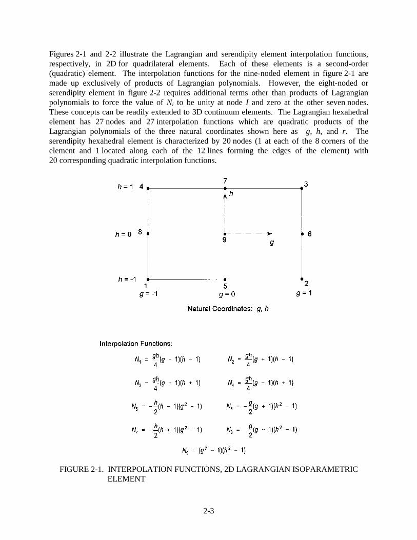
Figures 2-1 and 2-2 illustrate the Lagrangian and serendipity element interpolation functions, respectively, in 2D for quadrilateral elements. Each of these elements is a second-order (quadratic) element. The interpolation functions for the nine-noded element in figure 2-1 are made up exclusively of products of Lagrangian polynomials. However, the eight-noded or serendipity element in figure 2-2 requires additional terms other than products of Lagrangian polynomials to force the value of Ni to be unity at node I and zero at the other seven nodes. These concepts can be readily extended to 3D continuum elements. The Lagrangian hexahedral element has 27 nodes and 27 interpolation functions which are quadratic products of the Lagrangian polynomials of the three natural coordinates shown here as g, h, and r. The serendipity hexahedral element is characterized by 20 nodes (1 at each of the 8 corners of the element and 1 located along each of the 12 lines forming the edges of the element) with 20 corresponding quadratic interpolation functions.
FIGURE 2-1. INTERPOLATION FUNCTIONS, 2D LAGRANGIAN ISOPARAMETRIC ELEMENT
2-3

FIGURE 2-2. INTERPOLATION FUNCTIONS, 3D SERENDIPITY ISOPARAMETRIC ELEMENT
All of the isoparametric elements are integrated numerically. For many element types, the user has the option of selecting elements with full integration or reduced integration. The choice of order of integration is important, because it can have a significant affect on cost of the analysis and on the accuracy of the solution (Bathe 1982). Full integration means that the Gaussian integration employed will integrate the element stiffness matrix exactly if the determinant of the Jacobian matrix is constant over the element, i.e., if opposing sides for 2D elements or opposing faces for 3D elements are parallel. For reduced integration the integration scheme is one order less than that required to fully integrate the element stiffness matrix. Solution times may be significantly less with reduced integration resulting in considerable savings for large 3D models.
2-4

In problems where the predominant response mode is bending, fully integrated first-order elements may “lock”; i.e., the stiffness may be several orders of magnitude too great. Spurious shear stresses known as parasitic shear stresses are present. In these cases, a reduction in order of the numerical integration can lead to better results. The finite element displacement formulation overestimates the stiffness of the system; thus, by not evaluating the element stiffness matrices exactly, better results may be obtained if the error in the numerical integration compensates for the overestimation of the system stiffness. However, a possibility with reduced integration is a type of mesh instability known as hourglassing. For 2D and 3D reduced integration elements, the element stiffness matrix is rank deficient, causing problems with the solution if the element is not provided with sufficient stiffness restraint in the global assemblage of elements. When this occurs, the global stiffness matrix becomes ill-conditioned and, in some cases, singular. An hourglass mode does not result in strain (and therefore does not contribute to the energy integral) leading to spurious zero-energy displacement modes which behave like a rigid-body mode.
Hourglass modes for the first-order reduced integration quadrilateral and hexahedral elements can propagate through the mesh, and hourglassing can become be a serious problem. ABAQUS employs hourglass control for these elements in an attempt to suppress hourglassing. In effect, additional stiffness is artificially added to the system to restrain the hourglassing modes. Default hourglass stiffness values are based upon the elastic properties of the system. Values for these stiffnesses other than the default values may be specified by the user. The artific ial energy associated with the hourglass control stiffnesses must be much less than the total strain energy of the system. First-order reduced integration elements with hourglass control may perform satisfactorily for very fine meshes, but can be inaccurate for coarse meshes.
2.3 ELEMENT DESCRIPTIONS.
The ABAQUS element library contains a vast selection of element types and formulations. A basic understanding of the type of element and assumptions made in the formulation of the element is required before selecting an element for use in a finite element model. The following paragraphs contain brief descriptions of the 2D and 3D elements considered in this response and sensitivity study.
2.3.1 2D Element Descriptions.
Even though the purpose of this research was to develop a 3D finite element model for the rigid pavement system, it was instructive to conduct certain sensitivity studies in 2D. These 2D sensitivity studies were conducted using elements from the ABAQUS element library. The ABAQUS element library contains a large library of general shell elements for analysis of curved shell, plate bending, and membrane problems. For a flat plate subjected to both in-plane and transverse loads, the bending and membrane effects are uncoupled; thus, the total response can be obtained by superimposing the bending and membrane responses. In general this is not true of the shell element. The shell element is similar to a plate element, except that the midsurface of a general shell element can be curved. In this case the bending and membrane stresses are coupled, and it is no longer possible to superimpose the two conditions (Fagan 1992).
2-5

The basic assumption for thin-plate bending and shell elements is that the thickness, h, is small compared to the minimum in-plane dimension of the structure, L. Thus, the stress perpendicular to the midsurface of the plate or shell is zero, and material particles originally on a straight line perpendicular to the midsurface will remain on a strain line as the structure deforms. In the thin (or Kirchoff) theory, transverse shear deformations are neglected, and the straight line remains perpendicular to the midsurface during deformations. The rule of thumb is that for values of L/h >20, the Kirchoff assumptions hold. For case where the transverse shear deformations cannot be neglected, it can be shown that the transverse shear stresses τxz and τyz are distributed parabolically across the thickness of the plate or shell with the maximum value occurring at the midsurface (Timoshenko and Woinowsky-Krieger 1959).
Table 2-1 gives a description of the ABAQUS shell elements considered in this sensitivity study. These elements include first- and second-order finite elements with five or six degrees of freedom per node. All shell elements in ABAQUS employ a reduced integration scheme. Each of the elements with five degrees of freedom per node explicitly impose the Kirchoff shear constraints (i.e., transverse shear deformation is not allowed). Elements with six degrees of freedom per node, known as “shear flexible” elements, allow transverse shear deformations. When these elements are used for thin-shell applications, the default transverse shear stiffness (Gz) imposes the Kirchoff constraints approximately so that, in many cases, the results are not significantly different from the results from the thin-shell elements. Thus, ABAQUS calculates the default transverse shear stiffness as
5 5 Eh Gz=
6 Gh=
6 2(1+ µ )
(2.3)
where
G = shear modulus of shell h = thickness of shell E = modulus of elasticity of shell µ = Poisson’s ratio of shell.
Elements S4R and S8R are especially susceptible to hourglass displacement modes in the displacement components perpendicular to the shell surface. In general, the 8-node serendipity element is considered a good basic element for most shell problems. When reduced integration is employed (as is the case for all of the ABAQUS shell elements used in this study), shear locking is of no consequence. Although the reduced integration element can exhibit hourglassing, it too is nonconsequential because hourglass modes cannot propagate throughout the mesh (Schnobrich 1990).
2-6

TABLE 2-1. DESCRIPTION OF ABAQUS 2D SHELL ELEMENTS USED IN SENSITIVITY STUDY
Element Type General Description
Number of Nodes
Degrees of Freedom per Nodes Interpolation
No. of Gauss Points Notes on Usage
S4R Isoparametric shell element, reduced integration
4 (u, v, w, θx, θy, θz)
Linear 1 Subject to hourglassing, intended for thick-shell applications
S4R5 Isoparametric shell element, reduced integration
4 (u, v, w, θx, θy)
Linear 1 Subject to hourglassing, recommended for thin-shell applications
S8R Isoparametric brick element, reduced integration
8 (u, v, w, θx, θy, θz)
Serendipity quadratic
4 Intended for thick-shell applications
S8R5 Isoparametric shell element, reduced integration
8 (u, v, w, θx, θy)
Serendipity quadratic
4 Recommended for thin-shell applications
S9R5 Isoparametric shell element, reduced integration
8 (u, v, w, θx, θy)
Lagrangian quadratic
4 Recommended for thin-shell applications
6
5
6
5
5
2.3.2 3D Element Descriptions.
Table 2-2 contains a listing of the 3D hexahedral elements from the ABAQUS library considered in this study. Element types considered included both linear and quadratic elements employing both full and reduced integration. Furthermore, both Lagrangian and serendipity formulations were considered for the quadratic elements. Each element type features three translational degrees of freedom per node. The C3D27 and C3D27R elements are variable node elements; that is, the number of nodes can be reduced from 27 nodes per element down to 21 nodes per element (or any number between) by removing the interior node from each of the faces of the element as desired.
As is the case with 2D shell elements, fully integrated elements can exhibit locking where bending is the primary response mode. This is particularly true of the linear element. Reduced integration provides relief from locking but may lead to problems with hourglassing. However, for the quadratic elements, hourglassing is typically nonconsequential, because hourglass modes do not propagate throughout the mesh.
Solution times and the corresponding costs for 3D problems are considerably greater than for their 2D counterparts. This is due to the dramatic increase in the bandwidth and well as the increase in the time required to formulate the element stiffness matrices because of the time required to integrate in the third dimension (Schnobrich 1990).
2-7

TABLE 2-2. DESCRIPTION OF ABAQUS 3D HEXAHEDRAL ELEMENTS USED IN SENSITIVITY STUDY
Element Type General Description
Number of Nodes
Degrees of Freedom per Nodes Interpolation
No. of Gauss Points Notes on Usage
C3D8 Isoparametric brick element
8 (u, v, w)
Linear 8 Subject to parasitic shear stresses
C3D8R Isoparametric brick element, reduced integration
8 (u, v, w)
Linear 8 Subject to hourglassing
C3D20 Isoparametric brick element, reduced integration
20 3 (u, v, w)
Serendipity quadratic
27 May exhibit locking when used to analyze bending
C3D20R Isoparametric brick element, reduced integration
20 3 (u, v, w)
Serendipity quadratic
8 Subject to hourglassing, although rarely problematic
C3D27 Isoparametric brick element
21 27
3 (u, v, w)
Lagrangian quadratic
27 May exhibit locking when used to analyze bending
C3D27R Isoparametric brick element, reduced integration
21 27
3 (u, v, w)
Lagrangian quadratic
14 Subject to hourglassing, although rarely problematic
3
3
2-8

3. SINGLE-SLAB RESPONSE AND SENSITIVITY STUDIES.
3.1 BACKGROUND.
This chapter contains a discussion of response and sensitivity studies for single-slab models conducted with the finite element code ABAQUS. The purpose of these sensitivity studies was primarily to select the refinement of the discretization (referred to as the mesh fineness) and the approximations within the elements (choice of element type) for the 3D rigid pavement problem. This process involved producing a number of finite element models with varying mesh fineness and element types, solving those models to obtain approximate solutions, and observing the convergence trends for key response parameters such as bending stress, shear stress, and deflection. Where possible, these responses were compared to analytical solutions and experimental results. All discussions presented in this chapter are relevant to ABAQUS but would likely hold for any finite element code with identical element types and solution schemes.
First, a well-accepted analytical solution was chosen to check the accuracy of the approximations made by the various finite element models produced during the sensitivity studies. Because of the widespread acceptance and verification of Westergaard’s theory (Westergaard 1923, 1926, 1928, 1933, 1939, 1948), it was chosen for this study. For the sensitivity studies to be valid, the finite element models generated must be compatible with Westergaard’s assumptions. Thus, all sensitivity studies for this research were conducted for the general problem of an elastic plate resting on a bed of springs foundation considering interior or edge loading conditions. Solutions to Westergaard’s theory include Westergaard’s equations, Pickett and Ray (1951) response charts, and computerized solutions such as WESTER (Ioannides 1984). ILLI-SLAB (Tabatabaie-Raissi 1978, Ioannides 1984, Korovesis 1990) is perhaps the most widely used and verified 2D plate theory finite element solution for the rigid pavement problem. Thus, where possible, all finite element solutions were compared against a Westergaard theory solution obtained from WESTER. Also, an ILLI-SLAB solution, developed considering the user guidance given by Ioannides (1984), was used as a benchmark.
3.2 EXAMPLE PROBLEMS FOR SENSITIVITY STUDIES.
A set of example problems was selected for performing the sensitivity studies. These problems included three interior load cases and two edge load cases. Each case consisted of a 203.3-mm (8-in.) -thick elastic slab resting on a dense liquid foundation with a modulus of subgrade reaction k = 81.43 MPa/m (300 psi/in.). The elastic slab had a modulus of elasticity of E = 20,700 MPa (3,000,000 psi) and a Poisson’s ratio of� µ = 0.15.� The radius of relative stiffness, as defined by Westergaard (1926)
= 4� (3.1)k)2
3
(112 Eh
µ−
where k = modulus of subgrade reaction. These values yield a radius of relative stiffness of � = 653.1 mm (25.70 in.).
3-1

3.2.1 Interior Load Case I.
Figure 3-1 shows the configuration for Interior Load Case 1. The slab was square with the length of the sides set at L = 3.049 m (120 in.). The center of the slab was loaded with a uniform pressure of p = 6.895 MPa (100 psi) over a square area and the length of the sides of the loaded area being 609.8 mm (24 in.). An equivalent circular load would have a radius of a = 344.0 mm (13.54 in.); thus the dimensionless load size ratio is a/ � = 0.527. The total applied load was 256.2 kN (57,600 lb). The personal computer program WESTER, developed by Ioannides (1984), was used to obtain a Westergaard solution. Due to the very large size of the load, the Westergaard-type solution for Interior Load Case 1 may not be entirely accurate. For this case, the maximum interior bending stress predicted by Westergaard’s theory, which occurs beneath the centroid of the loaded area, was 4.434 MPa (643.2 psi); thus the maximum normalized bending stress can be expressed as
2 σ h2 4.434 MPa × (0.2033 m ) = 0.715 (3.2) =
P Interior Case I 0.2562 MN
The maximum deflection from the Westergaard theory, which also occurs beneath the centroid of the loaded area, is 0.8398 mm (0.00331 in.). The maximum deflection, expressed as a dimensionless quotient, was the following:
2 w k �2 0.0008398 m × 81.43 MPa/m × ( 0.6531 m ) = 0.114 (3.3) =
P Interior 0.2562 MN Case I
3.2.2 Interior Load Case II.
A second interior load case, shown in figure 3-2, was investigated. This load case was identical to Interior Load Case I, except that the size of the square loaded area decreased to 203.3 mm (8 in.) on a side. Thus, the magnitude of the load was total load was 28.47 kN (6400 lb) for Interior Load Case II. The equivalent radius for circular loaded area is a = 114.7 mm (4.51 in.), yielding a dimensionless load size ratio of a/ � = 0.175.
Again, WESTER was used to obtain the Westergaard solution for Interior Load Case II. For this case, the maximum bending stress was 0.8898 MPa (129.1 psi), yielding a maximum dimensionless bending stress of
2 σ h2 0.8898 MPa × (0.2033 m ) = 1.29 (3.4) =
P Interior Case II 0.02847 MN
3-2

p = 6.895 MPa (100 psi)k = 81.43 MPa/m (300 psi/in.)E = 20,700 MPa (3,000,000 psi)µ = 0.15h = 203.3 mm (8 in.)� = 653.1 mm (25.7 in.)
FIGURE 3-1. SYSTEM CONFIGURATION, INTERIOR LOAD CASE I
The maximum deflection predicted by Westergaard theory is 0.1010 mm (0.00397 in.), which expressed as a dimensionless quotient, was
2 wk � 2 0.0001010 m × 81.43 MPa/m × (0.6531 m ) = 0.123 (3.5) =
P Interior 0.02847 MN Case II
3-3

p = 6.895 MPa (100 psi)k = 81.43 MPa/m (300 psi/in.)E = 20,700 MPa (3,000,000 psi)µ = 0.15h = 203.3 mm (8 in.)� = 653.1 mm (25.7 in.)
FIGURE 3-2. SYSTEM CONFIGURATION, INTERIOR LOAD CASE II
3.2.3 Interior Load Case III.
A third interior load case, shown in figure 3-3, was studied. All slab parameters from Interior Load Case II were retained with the exception of the horizontal extent of the slab, which was varied from 2 � to 10 � . In all cases, the slab remained a perfect square. Therefore, the maximum bending stress and deflection as predicted by Westergaard’s theory are identical to those of Interior Load Case II.
3-4

p = 6.895 MPa (100 psi)k = 81.43 MPa/m (300 psi/in.)E = 20,700 MPa (3,000,000 psi)µ = 0.15h = 203.3 mm (8 in.)� = 653.1 mm (25.7 in.)
FIGURE 3-3. SYSTEM CONFIGURATION, INTERIOR LOAD CASE III
3.2.4 Edge Load Case I.
The edge load case considered in the sensitivity studies is illustrated in figure 3-4. The slab was rectangular with the maximum dimension of 3.049 m (120 in.) and the minimum dimension of 2.541 m (100 in.). A uniform pressure of p = 6.895 MPa (100 psi) was applied at the center of one edge of the slab over a square area and the length of the sides of the loaded area being 203.3 mm (8 in.). An equivalent circular load would have a radius of a = 114.7 mm (4.51 in.), yielding a dimensionless load size ratio of a/ � = 0.175. The magnitude of the load was total load was 28.47 kN (6400 lb).
3-5

3.049 m
p = 6.895 MPa (100 psi)k = 81.43 MPa/m (300 psi/in.)E = 20,700 MPa (3,000,000 psi)µ = 0.15h = 203.3 mm (8 in.)� = 653.1 mm (25.7 in.)
FIGURE 3-4. SYSTEM CONFIGURATION, EDGE LOAD CASE I
WESTER was used to obtain a Westergaard solution for the edge loading problem. The maximum bending stress, which occurs at the edge of the slab underneath the centroidal axis of the loaded area, was 1.719 MPa (249.3 psi) which can be expressed as the dimensionless quotient as
2 σ h2 1.719 MPa × (0.2033 m )
= 2.49 (3.6) = P Edge Case I
0.02847 MN
The maximum deflection predicted by Westergaard was 0.3028 mm (0.01192 in.). The dimensionless deflection is
2 wk � 2 0.0003028 m × 81.43 MPa/m × (0.6531 m ) = 0.369 (3.7) =
P Edge Case I 0.02847 MN
3-6

3.2.5 Edge Load Case II.
A plot of the system configuration for Edge Load Case II is shown in figure 3-5. The lengths of the sides of the square slab were varied from 2 � to 10 � . The load, slab thickness, slab elastic properties, and modulus of subgrade reaction were identical to that of Edge Load Case I; thus, the radius of relative stiffness of the system was identical and the expected bending stress and deflection remained unchanged from Edge Load Case I.
p = 6.895 MPa (100 psi)k = 81.43 MPa/m (300 psi/in.)E = 20,700 MPa (3,000,000 psi)µ = 0.15h = 203.3 mm (8 in.)� = 653.1 mm (25.7 in.)
FIGURE 3-5. SYSTEM CONFIGURATION, EDGE LOAD CASE II
3.3 RESPONSE AND SENSITIVITY STUDY RESULTS.
Some of the questions to be answered by the response and sensitivity study are summarized as the following:
a. What 3D hexahedron element is appropriate for the slab-on-grade problem?
b. What mesh fineness is required in the plane of the slab surface?
c. What mesh fineness is required in the plane of the slab thickness?
3-7

d. Should the analyst be concerned about transverse shear deformations for interior and edge load cases for rigid pavements?
e. What is the minimum slab dimension in the plane of the slab surface required to meet Westergaard’s assumption of a semi-infinite or infinite slab? How significant is this boundary effect for finite element modeling?
These issues are addressed in the remainder of this chapter.
3.3.1 Interior Load Case I.
Interior Load Case I was the most general load case studied and was primarily intended to study mesh fineness and element selection issues. Studies were conducted in both 2D and 3D. These studies are described and summarized below.
3.3.1.1 2D Convergence Studies.
Four finite element meshes representing different degrees of mesh fineness were generated. Table 3-1 is a summary of the results of these calculations. The degree of mesh fineness is characterized by the dimensionless ratio h/2a were h is the thickness of the slab and 2a is the minimum length of the side of an element. Figure 3-6(a) shows a diagram of the lengths of the sides of the 2D shell elements. Each of the finite element meshes are shown in figure 3-7.
TABLE 3-1. RESULTS OF 2D CONVERGENCE STUDY, INTERIOR LOAD CASE I
ABAQUS
h/2a Mesh Fineness
ILLISLAB S4R S4R5 S8R5
S8R (Default Gz)
S8R (100 x Default Gz) S9R5
Dimensionless Maximum Interior Bending Stress��σ�2/P
0.67 Coarse 0.804 0.575 0.575 0.804 0.805 0.802 0.716
1.33 0.751 0.695 0.694 0.748 0.748 0.751 0.727
2.67 0.739 0.722 0.722 0.735 0.735 0.739 0.730
4.00 Fine 0.736 0.727 0.727 0.733 0.733 0.736 0.733
Dimensionless Maximum Interior Deflection, wk � 2/P
0.67 Coarse 0.129 0.130 0.130 0.132 0.132 0.131 0.132
1.33 0.129 0.132 0.132 0.132 0.132 0.139 0.132
2.67 0.129 0.132 0.132 0.132 0.132 0.129 0.132
4.00 Fine 0.128 0.132 0.132 0.132 0.132 0.129 0.132
3-8

FIGURE 3-6. DEFINITION OF ELEMENT DIMENSIONS FOR DETERMINING MESH FINENESS
FIGURE 3-7. FINITE ELEMENT MESHES IN PLANE OF SLAB SURFACE, INTERIORLOAD CASE I
3-9

For each mesh the slab was modeled using double symmetry, i.e., both the x and y axis were axes of symmetry, thus reducing the memory requirements and computing time. The elements were all square and uniform throughout each mesh. Identical meshes were used for ILLI-SLAB and ABAQUS, with the exception that midside nodes were required for the quadratic shell elements in ABAQUS. For the nine-noded ABAQUS shell element, an additional node was required at the centroid of each element.
The Westergaard solution for this problem predicts a greater stress and a lessor deflection compared to the ILLI-SLAB solution. This is due to the quite large load size ratio (a/ � > 0.5) for this problem. In this case, the ILLI-SLAB solution is more accurate and should be used as the baseline calculation for this load case.
It is immediately apparent from table 3-1 that for both ILLI-SLAB and the ABAQUS shell elements that deflections converge much faster than stresses. The linear shell elements (S4R and S4R5) performed poorly for the coarser meshes, while the quadratic shell elements (S8R5, S8R, and S9R5) performed much better. The differences observed between the ABAQUS shell elements with six degrees of freedom per node (S4R and S8R) and their conjugate element with five degrees of freedom per node (S4R5 and S8R5, respectively) were small.
3.3.1.2 3D Convergence Studies.
A partial matrix of convergence studies was conducted in 3D for Interior Load Case I. The results of these studies are summarized in table 3-2. This load case was used to study the choice of element types for 3D modeling, the mesh fineness in the plane of the pavement surface, and the mesh fineness through the depth of the slab. As in the case of the 2D shell elements, the fineness of the mesh in the plane of the slab was characterized by the element aspect ratio in that plane defined by h/2a where 2a is the length of the smallest side of the element in the horizontal plane. Likewise, in the plane of the slab thickness, the fineness of the mesh was characterized by the aspect ratio h/2c, where 2c is the length of the smallest side of the element in the vertical plane. These dimensions are indicated in figure 3-6(b). In plan view the meshes were composed of square elements whose aspect ratios were identical to those shown in figure 3-7. Figure 3-8 shows a diagram of selected 3D meshes through the thickness of the slab.
The results in table 3-2 indicate that the linear hexahedral elements, both fully integrated (C3D8) and under integrated (C3D8R), under predict the dimensionless stress parameter for the rigid pavement problem. This is due to locking of the element. However, the responses of the quadratic elements (C3D20, C3D20R, C3D27, and C3D27R) are much better than those of the linear elements. Each of the serendipity formulation elements (C3D20 and C3D20R) and the Lagrangian elements (C3D27 and C3D27R) performed quite well. The convergence trends for dimensionless bending stress and dimensionless deflection are shown in figures 3-9 and 3-10, respectively. One of the primary distinctions between the serendipity and Lagrangian elements is in the amount of CPU time required to perform the calculations as illustrated in figure 3-11. The solution time for the C3D27 element is over two times that required for the C3D20 element. For both the C3D20R and C3D27R, use of reduced integration results in a reduction of CPU time by about 10 percent over its fully integrated counterpart.
3-10

3-11
TABLE 3-2. ULTS OF 3D CONVERGENCE STUDY, INTERIOR LOAD CASE I
ILLI-SLAB ABAQUS
h/2a (2D) h/2c C3D8 C3D8R C3D20 C3D20R C3D27 C3D27R
Dimensionless Stress at Center of Loaded Area (σyyh2/P)
0.67 0.751 1.0 0.414 0.431 0.754 0.751 0.753 0.750
1.5 0.476 0.505 0.754 0.755 0.752 0.751
2.0 0.509 0.545 0.753 0.757 0.752 0.752
1.33 0.739 1.0 -- -- -- -- -- --
1.5 -- -- -- -- -- --
2.0 0.582 0.571 0.746 0.744 0.746 0.745
2.00 0.736 1.0 -- -- 0.745 -- -- --
1.5 -- -- 0.745 -- -- --
2.0 0.597 0.575 0.745 0.742 0.745 0.743
Dimensionless Deflection at Center of Loaded Area (wk� 2/P)
0.67 0.129 1.0 0.128 0.146 0.131 0.131 0.131 0.131
1.5 0.124 0.137 0.131 0.131 0.131 0.131
2.0 0.123 0.134 0.131 0.131 0.131 0.131
1.33 0.129 1.0 -- -- -- -- -- --
1.5 -- -- -- -- -- --
2.0 0.130 0.135 0.131 0.131 0.131 0.131
2.00 0.128 1.0 -- -- 0.131 -- -- --
1.5 -- -- 0.131 -- -- --
2.0 0.132 0.135 0.131 0.131 0.131 0.131
CPU Time on CRAY Y-MP Computer, sec
0.67 -- 1.0 8.6 7.4 25.1 20.9 28.4 32.6
1.5 12.8 11.0 38.3 32.1 57.3 50.4
2.0 17.0 14.7 52.7 44.2 81.2 54.0
1.33 -- 1.0 -- -- -- -- -- --
1.5 -- -- -- -- -- --
2.0 57.6 60.4 180.2 225.3 298.8 268.7
2.00 -- 1.0 -- -- 202.2 -- -- --
1.5 -- -- 325.9 -- -- --
2.0 165.7 144.3 773.4 695.3 1636.6 1560.6
Table entries of “--” indicate that this computation was not performed or is not applicable.
RES

FIGURE 3-8. FINITE ELEMENT MESHES IN PLANE OF SLAB THICKNESS, INTERIOR LOAD CASE I
The results in table 3-2 show that increasing the mesh fineness in the plane of the slab thickness from h/2c = 0.67 (in this case, two elements through the slab thickness) to h/2c = 2 (four elements through the slab thickness) has a negligible affect on the accuracy of the solution for the quadratic hexahedron elements. Thus, at least three elements through the slab thickness is likely a good choice since it is desirable to maintain the element aspect ratios in all three dimensions to reasonable values.
3-12

FIGURE 3-9. DIMENSIONLESS BENDING STRESS, INTERIOR LOAD CASE I
FIGURE 3-10. DIMENSIONLESS DEFLECTION, INTERIOR LOAD CASE I
3-13

FIGURE 3-11. CPU TIME, SELECTED 3D RUNS, INTERIOR LOAD CASE I
3.3.1.3 Summary.
Figure 3-12 shows a comparison of dimensionless bending stress between ILLI-SLAB and the ABAQUS S8R (with both the default transverse shear stiffness and 100 times the default transverse shear stiffness) and C3D27R elements as a function of mesh fineness as measured by h/2a. It is apparent from this plot that the response of the S8R element most nearly matches that of ILLI-SLAB when the transverse shear stiffness is increased over that of the default value. The data in this plot also indicate that the C3D27R element predicts slightly greater stresses than either of the two ABAQUS models and ILLI-SLAB. Figure 3-13 shows a similar plot for dimensionless deflection. These data show that the deflection convergence curves for ABAQUS are completely flat, indicating that additional mesh fineness does not increase accuracy. It is of interest to note that the deflection of the C3D27R element lies between the two indicated curves for the S8R element.
Thus, it would appear that any of the quadratic hexahedron elements would perform successfully in a general, 3D model of the rigid pavement system. Strictly based upon indicated solution times, the C3D20R would appear to be the optimum element for this problem. However, other concerns (such as compatibility with interface and joint elements) make the C3D27R a more pragmatic choice for further model development.
3-14

FIGURE 3-12. DIMENSIONLESS BENDING STRESS SUMMARY, INTERIOR LOAD CASE I
FIGURE 3-13. DIMENSIONLESS DEFLECTION SUMMARY, INTERIOR LOAD CASE I
3.3.2 Interior Load Case II.
Interior Load Case II was studied to obtain a more direct comparison of the finite element solutions to the Westergaard interior load case. The finite element meshes used for Interior Load Case II are shown in figure 3-14. Three models were used with h/2a ratios of 2, 4, and 8, respectively. For each case a quarter-slab model was used, taking advantage of symmetric boundary conditions along both the x and y axes to enforce the interior loading condition. For the C3D27R model, the aspect ratio in the plane of the slab thickness was set at h/2c = 2. The results of these analyses are summarized in table 3-3.
3-15

FIGURE 3-14. FINITE ELEMENT MESHES IN PLANE OF SLAB SURFACE, INTERIOR LOAD CASE II
TABLE 3-3. RESULTS OF CONVERGENCE STUDY, INTERIOR LOAD CASE II
ABAQUS
Westergaard h/2a ILLI-SLAB S8R5 S8R5
(Default Gz) S8R
(100*Default Gz) C3D27R (h/2c = 2)
Dimensionless Bending Stress (σh2/P)
1.295 2 1.405 1.403 1.405 1.407 1.354
4 1.347 1.342 1.342 1.346 1.330
8 1.330 1.323 1.328 1.327 1.322
Dimensionless Deflection (wk � 2/P)
0.123 2 0.139 0.146 0.146 0.138 0.143
4 0.138 0.146 0.146 0.138 0.143
8 0.138 0.146 0.146 0.138 0.143
These data indicate that the finite element models considered tend to predict maximum interior bending stresses that are in reasonable agreement with those predicted by Westergaard when the mesh fineness in the plane of the slab surface is given by h/2a ≤ 4. For deflections, the results are virtually insensitive to mesh fineness over the ranges considered in this study. However, it should be noted that the deflections calculated from the finite element analyses are approximately 15 percent greater than those predicted by Westergaard, except for the S8R element with 100 Gz.
3.3.3 Interior Load Case III .
The lengths of the sides of the square slab were varied from 2 � to 10 � to investigate the effects of the slab dimensions on Westergaard’s assumption of an infinite slab using the S8R element with the ABAQUS default transverse shear stiffness. The finite element meshes used for Interior Load Case III are shown in figure 3-15. A quarter-slab model was used, taking advantage of
3-16

symmetric boundary conditions along both the x and y axes to enforce the interior loading condition. �Figure 3-16 summarizes the results of these calculations expressed as the ratios of the maximum stress calculated from the finite element method (σFEM) to the maximum Westergaard interior stress (σWestergaard). Based upon these calculations, one can conclude that the minimum slab dimensions required to approximate an infinite slab for the interior loading case is approximately L/ � = 6. Also, the commonly held rule of thumb for the transition between thin-and thick-plate theory of L/h ≈ 20 appears to be borne out by these calculations. Figure 3-17 shows a plot of the maximum deflection calculated from the finite element method (wFEM) to the maximum Westergaard interior deflection (wWestergaard). Similar conclusions can be drawn from this plot.
FIGURE 3-15. FINITE ELEMNET MESHES IN PLANE OF SLAB SURFACE, INTERIOR LOAD CASE III
3-17

FIGURE 3-16. STRESS RATIO, INTERIOR LOAD CASE III
FIGURE 3-17. DEFELCTION RATIO, INTERIOR LOAD CASE III
3.3.4 Edge Load Case I.
Edge Load Case I was developed to study the response of the finite element model for the edge load case. As with the interior load cases, ILLI-SLAB runs were made using identical meshes for
3-18

purposes of comparison. Based upon the results of the previously described interior load cases, the only ABAQUS 2D element considered for this load case was the S8R. However, the transverse shear stiffness of the element was varied to study its influence on the response of the model. A half-slab model was employed, taking advantage of symmetric boundary conditions along the x axis to enforce the edge loading condition. Figure 3-18 shows the finite element model developed for this purpose. The model consisted of square elements with an h/2a ratio of 4.
FIGURE 3-18. FINITE ELEMENT MESHES IN PLANE OF SLAB SURFACE, EDGE LOAD CASE I
3-19

Figure 3-19 shows dimensionless bending stresses from ABAQUS and ILLI-SLAB for Edge Load Case I plotted versus distance from the edge of the slab as a function of the transverse shear stiffness. These data show a perplexing result from ABAQUS; the stresses do not increase monotonically to the edge of the slab, but decrease near the edge. This finding disagrees with the ILLI-SLAB solution, which increases monotonically to the edge of the slab. Away from the edge of the slab, ILLI-SLAB and ABAQUS S8R agree quite well. In fact, as the transverse shear stiffness of the S8R element is increased, the response approaches that of ILLI-SLAB until at a transverse shear stiffness of 100 times the default the ABAQUS S8R response approximates the ILLI-SLAB response.
FIGURE 3-19. DIMENSIONLESS BENDING STRESS, EDGE LOAD CASE I
A 3D model was developed using the ABAQUS C3D27R element with three elements through the thickness of the slab (h/2c = 1.67). In the plane of the slab surface, the mesh was identical to that shown in figure 3-18. Figure 3-20 shows a plot of dimensionless bending stresses from ABAQUS and ILLI-SLAB plotted versus distance from the edge of the slab as a function of the transverse shear stiffness including the ABAQUS C3D27R model. Also shown in the plot are the responses predicted by the ABAQUS S8R element for three values of transverse shear stiffness: one, two, and 100 times the ABAQUS default values. Interestingly enough, the ABAQUS C3D27R response more nearly matches the response of the S8R element with the default transverse shear stiffness than the ILLI-SLAB response. In fact, the 3D model matches the response from the S8R model very closely when the default transverse shear stiffness is twice the default value.
3-20
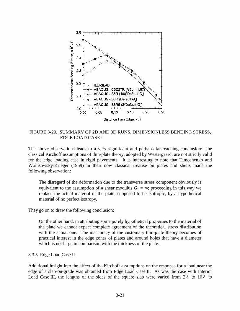
FIGURE 3-20. SUMMARY OF 2D AND 3D RUNS, DIMENSIONLESS BENDING STRESS, EDGE LOAD CASE I
The above observations leads to a very significant and perhaps far-reaching conclusion: the classical Kirchoff assumptions of thin-plate theory, adopted by Westergaard, are not strictly valid for the edge loading case in rigid pavements. It is interesting to note that Timoshenko and Woinsowsky-Krieger (1959) in their now classical treatise on plates and shells made the following observation:
The disregard of the deformation due to the transverse stress component obviously is equivalent to the assumption of a shear modulus Gz = ∞; proceeding in this way we replace the actual material of the plate, supposed to be isotropic, by a hypothetical material of no perfect isotropy.
They go on to draw the following conclusion:
On the other hand, in attributing some purely hypothetical properties to the material of the plate we cannot expect complete agreement of the theoretical stress distribution with the actual one. The inaccuracy of the customary thin-plate theory becomes of practical interest in the edge zones of plates and around holes that have a diameter which is not large in comparison with the thickness of the plate.
3.3.5 Edge Load Case II.
Additional insight into the effect of the Kirchoff assumptions on the response for a load near the edge of a slab-on-grade was obtained from Edge Load Case II. As was the case with Interior Load Case III, the lengths of the sides of the square slab were varied from 2 � to 10 � to
3-21

investigate the effects of the slab dimensions on Westergaard’s assumption of an infinite slab using the S8R element with two values of the transverse shear stiffness: the default Gz, and 100 times the default Gz. The finite element meshes used for Edge Load Case II are shown in figure 3-21. A half-slab model was used, taking advantage of symmetric boundary conditions along the x axis to enforce the edge loading condition.
FIGURE 3-21. FINITE ELEMENT MESHES IN PLANE OF SLAB SURFACE, EDGE LOAD CASE II
3-22

The results of these analyses are shown in figures 3-22 and 3-23 as plots of dimensionless bending stress versus distance from the edge of the joint expressed as a function of � . In figure 3-22 the S8R transverse shear stiffness was set to the ABAQUS default value. Clearly, the maximum stress occurs at a distance of about 0.1 � from the edge of the slab for all values of L. Only for the case where L = 2 � is the response significantly different. Figure 3-23 is a similar plot for the case where the transverse shear stiffness was set to 100 times the default Gz. In this case, each of the response curves increase monotonically to the edge of the slab, as predicted by Westergaard and thin-plate finite element programs such as ILLI-SLAB. Again, the response is significantly different for the case where L = 2 � .
Figures 3-24 and 3-25 show similar curves for dimensionless deflection versus distance from the edge of the slab for the two values of transverse shear stiffness investigated. These curves indicate that deflections are not significantly influenced by the choice of transverse shear stiffness. Also, it can be observed that the deflection response is essentially the same for all curves were L/ � ≥ 6.
Based upon these observations, it can be stated that, like the interior load case, the ratio of the minimum slab dimension to the radius of relative stiffness of at least 6 is required to model a semi-infinite slab. It can also be concluded that the magnitude and distribution of bending stresses near the edge of a slab are strongly dependent upon the transverse shear stiffness of the slab, while deflections are not sensitive to this parameter.
FIGURE 3-22. DIMENSIONLESS BENDING STRESS, DEFAULT TRANSVERSE SHEAR STIFFNESS, EDGE LOAD CASE II
3-23

FIGURE 3-23. DIMENSIONLESS BENDING STRESS, 100 TIMES DEFAULTTRANSVERSE SHEAR STIFFNESS, EDGE LOAD CASE II
FIGURE 3-24. DIMENSIONLESS DEFLECTION, DEFAULT TRANSVERSE SHEARSTIFFNESS, EDGE LOAD CASE II
3-24

FIGURE 3-25. DIMENSIONLESS DEFLECTION, 100 TIMES DEFAULT TRANSVERSE SHEAR STIFFNESS, EDGE LOAD CASE II
To develop further insight into the effect of the transverse shear stiffness on the edge loading response, a set of finite element calculations were performed to determine the limiting value of L/h for which thin-plate theory was acceptable for the edge load case. Figure 3-26 shows the result of these analyses. From these data, it appears that for L/h > 100, the effects of transverse shear stiffness on the edge loading response is negligible. Thus for any practical rigid pavement, the edge stress is influenced by the assumption of the Kirchoff plate theory.
A special 3D finite element calculation was conducted to study the distribution of transverse shear stresses throughout the slab. The mesh in the plane of the slab surface was identical to that used in Edge Load Case I with h/2a ratio set to 4. Four elements were used across the thickness of the slab so that the slab’s midsurface would be located at an element boundary. The load was identical to that described for Edge Load Cases I and II.
These results indicate the magnitude of the maximum value of τxz is approximately 20 percent of the magnitude of the maximum edge stress in the slab. The maximum value occurs just to the right edge of the loaded area near the centerline of the slab. The magnitude of the maximum value of τyz is approximately 30 percent of the magnitude of the maximum edge stress in the slab. The maximum value occurs near the edge of the free edge of the slab in the vicinity of the loaded area.
Figure 3-27 shows a cross section of the distribution of τyzh2/P through the thickness of the slab
near where its maximum value occurs. These data show that the transverse shear stress is distributed in a manner that is very nearly parabolic with the maximum value occurring at the slab’s midsurface. Thus, the finite element solution agrees with the theorized distribution of transverse shearing stresses across the slab.
3-25

FIGURE 3-26. EFFECT OF SLAB WIDTH TO DEPTH RATIO ON EDGE STRESSES
Sla
b T
hick
ness
FIGURE 3-27. FINITE ELEMENT DISTRIBUTION OF τxzh2/p THROUGH SLAB
THICKNESS
3-26

Experimental data to confirm the above observations are inconclusive. Full-scale accelerated test tracks as well as small-scale model tests conducted by the Corps of Engineers have indicated that the Westergaard analytical model overestimates the stresses and strains experienced in pavement (Rollings and Pittman 1992). Similar trends were found on small-scale model tests conducted by the Corps in the 1950’s. Figure 3-28 shows results from small-scale model tests conducted by the Corps of Engineers (1954). These data indicate that the Westergaard theory solution is conservative for both edge and interior load cases. In figure 3-29, the ratio of the Westergaard theory stresses to the experimental stresses is shown for both interior and edge loads over a range of a/ � . For these experiments, the discrepancy between theoretical and experimental stresses for the edge load case was less than that for the interior load case. However, two factors may have led to some errors in this data:
a. Stresses were not directly measured. Strains were measured by resistance strain gages bonded to the slab. For the edge load case, the strain gages were located at some finite distance from the edge, and the strains were extrapolated to the edge. This is equivalent to assuming that the Kirchoff theory applies.
b. The modulus of subgrade reaction of the rubber foundation used in these tests was estimated from the volume of the deflection basin produced by an edge loading and an interior loading. This method, at best, gives a composite estimate of the modulus of subgrade reaction but may lead to errors in the calculation of theoretical stresses.
FIGURE 3-28. THEORETICAL AND EXPERIMENTAL DIMENSIONLESS BENDING STRESS FROM SMALL-SCALE MODEL STUDIES
3-27

FIGURE 3-29. RATIO OF THEORETICAL TO EXPERIMENTAL BENDING STRESS FROM SMALL-SCALE MODEL STUDIES
3-28
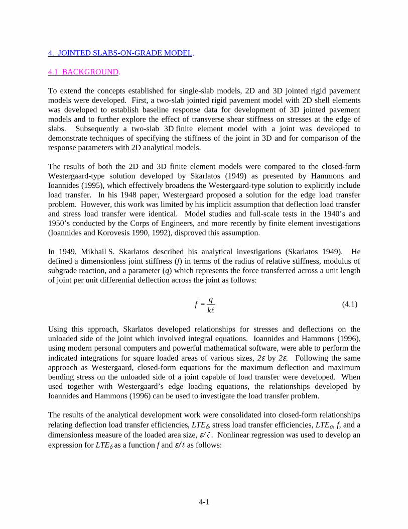
�
4. JOINTED SLABS-ON-GRADE MODEL.
4.1 BACKGROUND.
To extend the concepts established for single-slab models, 2D and 3D jointed rigid pavement models were developed. First, a two-slab jointed rigid pavement model with 2D shell elements was developed to establish baseline response data for development of 3D jointed pavement models and to further explore the effect of transverse shear stiffness on stresses at the edge of slabs. Subsequently a two-slab 3D finite element model with a joint was developed to demonstrate techniques of specifying the stiffness of the joint in 3D and for comparison of the response parameters with 2D analytical models.
The results of both the 2D and 3D finite element models were compared to the closed-form Westergaard-type solution developed by Skarlatos (1949) as presented by Hammons and Ioannides (1995), which effectively broadens the Westergaard-type solution to explicitly include load transfer. In his 1948 paper, Westergaard proposed a solution for the edge load transfer problem. However, this work was limited by his implicit assumption that deflection load transfer and stress load transfer were identical. Model studies and full-scale tests in the 1940’s and 1950’s conducted by the Corps of Engineers, and more recently by finite element investigations (Ioannides and Korovesis 1990, 1992), disproved this assumption.
In 1949, Mikhail S. Skarlatos described his analytical investigations (Skarlatos 1949). He defined a dimensionless joint stiffness (f) in terms of the radius of relative stiffness, modulus of subgrade reaction, and a parameter (q) which represents the force transferred across a unit length of joint per unit differential deflection across the joint as follows:
f =q
(4.1)k
Using this approach, Skarlatos developed relationships for stresses and deflections on the unloaded side of the joint which involved integral equations. Ioannides and Hammons (1996), using modern personal computers and powerful mathematical software, were able to perform the indicated integrations for square loaded areas of various sizes, 2ε by 2ε.� � Following the same approach as Westergaard, closed-form equations for the maximum deflection and maximum bending stress on the unloaded side of a joint capable of load transfer were developed. When used together with Westergaard’s edge loading equations, the relationships developed by Ioannides and Hammons (1996) can be used to investigate the load transfer problem.
The results of the analytical development work were consolidated into closed-form relationships relating deflection load transfer efficiencies, LTEδ, stress load transfer efficiencies, LTEσ, f, and a dimensionless measure of the loaded area size, ε/ � . Nonlinear regression was used to develop an expression for LTEδ as a function f and ε/ � as follows:
4-1

�
1 LTEδ =
ε 0.214- 0.18
� (4.2)
3 - log f 1-1+ log 1.180
Likewise, nonlinear regression was used to develop an expression for LTEδ as a function of LTEσ
and ε/ � . The following regression formula was obtained:
ε 7 3 2 ε 1206 + 37
LTEσ - 69 3 LTEσ � �
LTEδ = (4.3) ε ε 29
37 - 15
LTEσ41+ 68 �
LTEσ + 0
Nonlinear regression was used to develop an expression for LTEσ�as a function of ε/ � and����δ. The functional form of this regression algorithm was arbitrary from an engineering viewpoint and was selected from among a large number of choices investigated. The resulting algorithm was obtained:
ε 0
4. ε 8 2
10.14 + 4.0
LTEδ - 3 + 3.9
LTEδ � �
LTEσ = (4.4) ε 5.7
�
821.03+ 4 - 20.9 LTEδ
These relationships, based upon sound analytical principles, provide a complete solution for the load transfer problem in jointed rigid pavements in a form that is convenient for routine engineering calculations.
4.2 REPRESENTATION OF THE JOINT STIFFNESS.
The analytical work of Ioannides and Korovesis (1992) using ILLI-SLAB led them to conclude that the response of both aggregate interlock and doweled joints can be represented by the concepts of dimensionless joint stiffness. This conclusion, verified experimentally by small-scale model studies conducted by the Corps of Engineers in the 1950’s as reanalyzed in this study, eliminates the need to explicitly model dowels in finite element models. Coupled with the analytical developments of Skarlatos (1949), as presented by Ioannides and Hammons (1996), a powerful, yet simple, way of characterizing the dimensionless joint stiffness for finite element modeling emerges.
Selection of an appropriate ABAQUS finite element spring model for use in modeling the interaction of nodes across a joint was required. The ABAQUS element library contains a
4-2

collection of three simple spring models, each having its own unique properties. The SPRINGA element is an axial spring between two nodes whose line of action is the line joining the two nodes. The SPRING2 element allows the user more control over the line of action of the spring than the SPRINGA element by acting only a user-specified direction. The third simple spring element, the SPRING1 element, is a spring between a node and ground (a fixed, unmoveable fictitious node) which acts in a fixed, user-specified direction.
For each of these element types, the force-displacement relationship may be linear or nonlinear. For a linear force-displacement relationship, the user simply inputs the spring constant. For a nonlinear spring, the user must input a table containing ordered pairs of force-displacement data. ABAQUS then linearly interpolates between the input values to obtain a complete nonlinear description of the force-displacement relation of the spring.
ABAQUS also includes a more general spring and dashpot element called the JOINTC element. The JOINTC element, more formally known as flexible joint element, models the interaction between two nodes which may have internal stiffness or damping. The stiffness and damping properties, which may be linear or nonlinear, are defined by the user in three orthogonal directions. In a static analysis, damping is of no consequence and may be ignored; therefore, the JOINTC element reduces to a general spring element which may have a user-defined stiffness value in three orthogonal directions. Nonlinear force-displacement relationships for the JOINTC element are input by the user in a manner identical to that for the simple spring elements.
The stiffness of the joint in most finite element codes for rigid pavement analysis (for example ILLI-SLAB (Tabatabaie 1978, Ioannides 1984, Korovesis 1990)) consists of springs which have stiffness in the vertical direction only. Following this pattern, the interaction between nodes across a joint in ABAQUS could be modeled using the SPRING2 element. In the simplest case, the stiffness of the JOINTC element could be specified to be in the vertical direction only, reducing its effect to that of the SPRING2 element. However, the additional capabilities of the truly general 3D JOINTC element render it an attractive alternative to the more limited SPRING2 element. For example, for future research studies in which dynamic analysis may be considered or for environmental analysis in which temperature and moisture gradients are important, the JOINTC element offers some attractive capabilities. Based upon these considerations, the JOINTC element was selected for use in this study. However, where the stiffness of the JOINTC element is limited to only a single direction and damping is ignored, the simpler SPRING2 element would give identical results.
For an aggregate interlock load transfer mechanism, the joint stiffness is prescribed by the parameter q, which defines the force transmitted per unit length along the joint per unit differential deflection across the joint. This term is identical to the AGG term defined in ILLISLAB. For the dowel load transfer mechanism, q is defined as
D q= (4.5)
s where s is the dowel spacing.
4-3

The value of D depends upon the vertical stiffness caused by the support of the concrete, called the dowel-concrete interaction (DCI), and a vertical stiffness caused by beam bending. These two spring stiffnesses are summed as springs in series as follows:
1D=
1+
1 (4.6) DCI 12C
The value of DCI is based on assuming the dowel to be a beam on a spring foundation and is given by the following relationship:
34 βDCI =
(2+ βω ) Ed I d (4.7)
where ω is the width of the joint opening. The term β is identical to that used by Friberg (1940)
β = 4
d d
d
I E4 K (4.8)
where K is the modulus of dowel support.
The term C in equation 4.6 is defined by the relationship
C= Ed I d
ω3(1+ φ ) (4.9)
where
12Ed I dφ = Gd Azω 2 (4.10)
Gd is the shear modulus of the dowel bar as defined by
EdGd =
2(1+ µ d ) (4.11)
The term Az is the effective cross-sectional area in shear and is assumed to be 0.9 times the circular area as follows:
A z= 0.9 π d2 (4.12) 4
4-4

Once q has been established, it is necessary to distribute the stiffness to the nodes along the joint in a rational manner. One method of allocating the stiffness to the nodes is by using the concept of contributing area, which is commonly used in structural analysis. In this method the stiffness values assigned to each node, κ, are determined based upon the length (in 2D) or area (in 3D) that contributes to the stiffness of the node. For equally spaced nodes in a 2D model, the nodes along a joint may be categorized into one of two types: interior nodes or edge nodes. Edge nodes are those which occupy the ends of the joint, while all other nodes are interior nodes. Based upon the concepts of contributing area, the stiffness of the interior nodes must be twice that of the edge nodes. If the length of the joint is given by λ, and the number of nodes along the joint (for a 2D model) is given by N, then
κ =qλ
(4.13)2(N -1)
and
κ interior = 2κ (4.14)
κ edge= κ
For 3D finite element models, the nodes along the face of the solid model at a joint must be categorized into three types: corner, edge, and interior nodes. Corner nodes are those nodes which occupy the four corners of the face, while edge nodes are all other nodes on the edge of the face. Interior nodes make up the remainder of the nodes. If the spacing of the nodes on the face of the joint is uniform, the unit stiffness value is given by
κ =qλ
(4.15)4( N R - 1)( NC - 1)
where
NR = the number of rows of nodes on the face of the joint NC = number of columns of nodes on the face of the joint
The complete development of equation 4.15 is given in appendix A. Using the concept of contributing areas, the following stiffness can be assigned to each type of node:
κ = κcorner
κ edge = 2κ (4.16)
κ interior = 4κ
A simply-supported beam with a uniformly distributed load (figure 4-1) was used to investigate the behavior of the JOINTC element. The material properties chosen for the beam were E = 27,600 MPa and µ = 0.18. The maximum deflection of this beam, calculated from the beam
4-5

theory, is 0.906 m. The beam was modeled with C3D27R elements. Three cases were explored. First, the beam was modeled as a monolith elastic solid. For this case ABAQUS predicted a maximum deflection (δES) of 0.913 m, approximately 99 percent of that expected from beam theory.
FIGURE 4-1. SIMPLY-SUPPORTED BEAM PROBLEM TO TEST JOINTC ELEMENT
For the second case, the beam was split into two parts at its centerline, and the nodes across the joint were joined with JOINTC elements, as indicated in the inset labeled “DETAIL A” in figure 4-1. Values of q ranging from 103 to 107 MN/m/m were selected, and the individual spring constants, κ, were calculated using equations 4.15 and 4.16. Because it was desired to transfer both shear and bending moments across the joint, the JOINTC elements were assigned identical stiffnesses in all three degrees of freedom. These models were submitted as ABAQUS runs and the maximum corresponding deflections (δJOINTC) extracted from the output fi les. The results of these computations, presented in figure 4-2, indicate that as q approaches infinity the deflection approaches that calculated for the case in which the beam was monolithic. This could be true only if the JOINTC elements were effective in transferring shear and bending moments across a joint.
In the third and final case investigated for this beam problem, the JOINTC elements were replaced with a type of kinematic restraint known in ABAQUS as multipoint constraints (MPC). MPCs are used to specify constraints between nodes. These constraints may be quite general, and a full description is not warranted here. The type of MPC option chosen for the beam problem is referred to as a “TI E”; that is, all active degrees of freedom are set equal at two nodes. It is intended to be used to join two parts of a mesh when corresponding nodes are to be fully connected. The results from this analysis, as expected, indicated that the maximum deflection was 0.913 m, identical to that from the monolithic elastic solid beam. Thus, MPCs with the TIE option invoked may be used to rigidly connect two bonded elastic bodies.
4-6

FIGURE 4-2. RESULTS FROM SIMPLY-SUPPORTED BEAM WITH JOINTC ELEMENT
4.3 EXAMPLE PROBLEM.
An example jointed slabs-on-grade problem was developed to verify the usefulness of the proposed ABAQUS model. The structural response obtained from the finite element solutions was compared with the closed-form, Westergaard-type solution for load transfer developed by Ioannides and Hammons (1996). The concepts of the dimensionless joint stiffness were used to determine the structural parameters for the joint.
Two 6-m square slabs-on-grade separated by a doweled joint were chosen for the example problem. Table 4-1 contains of summary of the material and structural parameters for this problem. Where applicable, the germane equation numbers have been listed in the table. The material parameters assumed in this problem were typical of those commonly used in analysis. Similarly, the joint structural parameters were selected to be representative of those which might be expected in airport pavements. The load consisted of a uniformly pressure of p = 2.5 MPa distributed over an area of 0.06 m2. The structural response calculated from the Westergaardtype solution is also tabulated in table 4-1.
A 2D shell element model of the example problem was developed to obtain response parameters for comparison with 3D models and to study the effect of the Kirchoff assumptions on load transfer at a joint. Figure 4-3 shows a plot of the finite element mesh used for this problem along with the material and structural properties assumed in the analysis. The ABAQUS shell element used in this model was the S8R element. The shell elements were supported on a bed of springs using the ABAQUS “FOUNDATION” option. Because calculations using this element are relatively inexpensive on the Cray computer, a fine mesh was employed to mitigate any effects from mesh fineness concerns.
4-7

--
--
--
--
--
--
--
--
--
--
--
-- --
--
--
--
--
TABLE 4-1. MATERIAL AND STRUCTURAL PARAMETERS, JOINTED SLABS-ON-GRADE EXAMPLE PROBLEM
Parameter Equation No. Dimensions Value
Slabs-on-Grade Material Parameters
Es F/L2 27,600 MPa
µs — — 0.15
k F/L3 115 MPa/m
Slabs-on-Grade Structural Parameters
h L 0.432 m
� 3.1 L 1.133 m
a L 0.138 m
ε L 0.123 m
ε/ � — — 0.108
Joint Material Parameters
Ed F/L2 200,000 MPa
µd — — 0.30
K F/L3 407,000 MPa/m
Joint Structural Parameters
s L 0.457 m
d L 0.0508 m
Id L4 0.0327×10⁻⁶ m4
Az 4.12 L2 1.82×10⁻³ m2
Gd 4.11 F/L2 76,900 MPa
ω — L 0.00254 m
φ 4.10 867
C 4.9 F/L 4600 MN/m
β 4.8 L-1 16.8 m-1
DCI 4.7 F/L 604 MN/m
D 4.6 F/L 597 MN/m
f = D/sk � 10.0
q = D/s F/L2 1300 MN/m/m
Structural Response Parameters
LTEδ 1.4 0.828
LTEσ 1.5 0.281
LT 1.6 0.220
4-8

Two Slabs at 6 m Each JOINT
E = 27,600 MPa L/h = 13.89 p = 2.5 MPa µ = 0.15 L/ � = 5.30 A = 0.06 m2
h = 0.432 m q = 1300 MN/m/m Ρ = 0.15 MN k = 115 MPa/m kinterior = 65 MN/m ε = 0.123 m � = 1.133 m kedge = 32.5 MN/m ε/ � = 0.108 Gz = 4320 MPa
FIGURE 4-3. FINITE ELEMENT MESH FOR 2D JOINTED RIGID PAVEMENT MODEL
Analyses were conducted using several multiples of the default transverse shear stiffness to investigate the effect this parameter might be having on load transfer. Figure 4-4 shows plots of dimensionless bending stress versus distance from the joint. The loaded slab was to the left of the joint. This plot shows that transverse shear stiffness has the same effect near a joint as near a free edge. For values of transverse shear stiffness less than approximately 100 times the ABAQUS default value, the maximum transverse bending stress values were predicted to be at some finite distance from the joint rather than at the joint. This phenomenon is evident on both the loaded and unloaded sides of the joint.
The influence of the transverse shear stiffness on the commonly used measures of joint response is indicated in figure 4-5. Here, load transfer was calculated by forming the ratios of the slab responses (deflection or stress) at the joint, not at the peak values. Also shown on these plots are the Skarlatos solutions. It can be seen in figure 4-5 that LTEδ converges to the Skarlatos solution from below as transverse shear stiffness increases, while LTEσ and LT converge from above. It should be recognized that the Skarlatos solution is based upon Westergaard’s theory and implicitly assumes that the slab can be modeled as a thin plate. Deflection load transfer effic iency for values of default transverse shear stiffness greater than approximately 10 times the ABAQUS default values agrees well with the Skarlatos solution. However, load transfer and stress load transfer efficiencies predicted by the finite element model are consistently greater than those predicted by Skarlatos.
4-9

FIGURE 4-4. BENDING STRESSES PREDICTED BY 2D FINITE ELEMENT MODEL OF A JOINTED PAVEMENT
A 3D finite element model using ABAQUS C3D27R elements was created and executed. The model was identical in plane view to the 2D shell element model shown in figure 4-3. Four elements were used through the depth of the model. The lowest layer of elements was supported on a bed of springs using the ABAQUS “FOUNDATION” option. All material and structural parameters were the same as those used for the 2D shell element model (as described in figure 4-3). However, one exception should be noted. In 3D the individual spring constants were assigned according to equations 4.15 and 4.16 as follows:
κ corner= 2.301MN/m
κ edge= 4.063 MN/m (4.17)
κ interior = 8.125MN/m
4-10

0.1 1 10 100
FIGURE 4-5. COMPARISON OF JOINT RESPONSE PARAMETERS, 2D FINITE ELEMENT MODEL
Figure 4-6 shows the a plot of the dimensionless bending stress from the 3D model along with selected data from the 2D shell element model. On the loaded side of the joint, the 3D model predicted lower stress than the 2D models. As was the case for a free edge, the 3D model predicts that the maximum stress does not occur at the joint, but some small distance away from
4-11

the joint. The higher bending stresses predicted by the 2D model were believed to be an artifact of the 2D shell element formulation, and the 3D bending stresses are likely more accurate.
FIGURE 4-6. COMPARISON OF BENDING STRESSES PREDICTED BY 2D AND 3D FINITE ELEMENT MODELS OF A JOINTED PAVEMENT
The 3D finite element model was repeatedly executed, varying the value of q to get a range of responses. These data were then plotted against results from the relationships developed by Ioannides and Hammons (1996) from the Skarlatos model. The results of these comparisons are presented in figures 4-7 and 4-8. The ABAQUS 3D example problem is indicated in each plot.
These figures indicate that over a wide range of values of joint stiffnesses and load transfer efficiencies, the trends predicted by the 3D finite element models are in agreement with those predicted by the closed-form solution. From figure 4-8, it can be observed that the Skarlatos model predicts lower values of stress load transfer efficiencies over a range of deflection load transfer efficiencies from 0.6 to 0.9, the range commonly encountered in airport pavements. Thus, the Skarlatos closed-form solution is more conservative than the finite element solutions over this range of values. This conclusion is also confirmed by the results from the example problem as shown in figure 4-5. However for many, if not all, heavily loaded rigid airport pavement slabs, the slab thickness is great enough that thin-plate theory is not strictly valid. For these slabs, load transfer is greater than that predicted by thin-plate theory.
4-12

FIGURE 4-7. COMPARISON OF 3D FINITE ELEMENT MODEL WITH CLOSED-FORM SOLUTION, DIMENSIONLESS JOINT STIFFNESS VERSUS DEFLECTION LOAD TRANSFER EFFICIENCY
FIGURE 4-8. COMPARISON OF 3D FINITE ELEMENT MODEL WITH CLOSED-FORM SOLUTION, STRESS LOAD TRANSFER EFFICIENCY VERSUS DEFLECTION LOAD TRANSFER EFFICIENCY
4-13/4-14

5. CONTACT AND FRICTION MODELING.
5.1 PROBLEM STATEMENT.
In a rigid pavement structure, the interface between the slab and base course may be bonded, debonded, or perhaps some condition in between. In the bonded case, full strain compatibility is enforced between the slab and base course. In the debonded case, movement along the interface between the two bodies may be resisted by friction (aggregate interlock). If the slab and base are debonded, gaps between them are a possibility, particularly in the vicinity of a loaded joint.
Contact interaction problems pose a challenge for the finite element modeler. When two solid bodies touch, a contact stress will be transmitted across the common surface. If there is friction between the two surfaces, a shear stress will also be present. The contact areas must be determined, and then the normal and shearing stresses transmitted through the contact area must be calculated. This gives rise to a highly nonlinear problem which requires an iterative solution procedure.
5.2 CONTACT AND FRICTION OPTIONS IN ABAQUS.
Two methods of modeling the mechanical interaction between element faces in ABAQUS are germane to the rigid pavement problem. The first of these methods involves the use of interface elements, referred to in ABAQUS as “INTER” elements, for contact and friction analysis. These elements are formulated to calculate the contact direction, contact area, and the normal and shear stresses transmitted across the contact surface. For 3D problems, three INTER elements are available in the ABAQUS element library: the INTER4 element, intended for use with 8-node hexahedral elements and 4-node shell elements; the INTER8 element, intended for use with 20-node hexahedral elements and 8-node shell elements; and the INTER9 element, intended for use with 21- to 27-node hexahedral elements and 9-node shell elements. Use of the INTER8 element is discouraged because uniform pressure on the 8-node surface produces negative contact forces at the corner nodes. The use of INTER elements is tedious, since they require the creation of zero-thickness elements along the contact interface.
The second method of modeling the contact and friction between two bodies is the ABAQUS contact interaction option. This option, recently added to ABAQUS, is more convenient than the INTER element because creation of additional elements is not required. The two surfaces which may be in contact are defined by the user along with a choice of several friction models. Because of negative contact forces which arise at the corners of elements with 8 nodes on a face, the use of contact interaction for 20-node hexahedral elements is not recommended. For purposes of this research, a simple Coulomb friction model will be adopted.
For both the INTER elements and the contact interaction option, the selection of boundary conditions at the interface is important to avoid certain numerical solver problems. Over constraint of the model results in “zero pivot” and “numerical singularity” warning messages from the solver and in most cases leads to an abnormal termination of the analysis. Because the contact interaction provides a kinematic constraint, these errors occur when two nodes on either
5-1

side of a contact surface are constrained with redundant kinematic boundary conditions. Figure 5-1 shows examples of an overconstrained and a nonoverconstrained contact surface problem.
FIGURE 5-1. EXAMPLE OF OVERCONSTRAINT FOR CONTACT PROBLEM
5.3 SIMPLE EXAMPLE PROBLEM.
Figure 5-2 shows a simply-supported beam problem investigated using the friction and contact capabilities in ABAQUS. The beam was loaded with a uniformly distributed load of 1 MN/m and was assigned the elastic constants E = 27,600 MPa and µ = 0.18. The symmetry of the problem was used to model only half of the beam. The beam was split into two parts along its neutral axis, and various friction values were assigned to the contact surface along the neutral axis. The beam was modeled using C3D27R elements, while both the INTER9 elements and the contact interaction element were used (in separate analyses) to model the contact and friction at the neutral axis. The maximum deflection of this beam (if it were monolithic) predicted by beam theory is 0.906 m.
FIGURE 5-2. SIMPLY-SUPPORTED BEAM PROBLEM TO TEST CONTACT INTERACTION FEATURES OF ABAQUS
5-2

Results from these analyses normalized by the predictions from beam theory are plotted in figure 5-3. For both of the investigated methods of modeling and friction, deflections calculated by the finite element method approach that predicted by beam theory as the coefficient of friction becomes large. The results also indicate that the contact interaction option predicts deflections closer to the theoretical deflection for values of the coefficient of static friction greater than approximately ten. Because the contact interaction method is easier to use than interface elements and because the contact interaction method appears to be slightly more accurate than the interface element method, it is recommended that the contact interaction method should be used to model contact and friction where required.
FIGURE 5-3. RESULTS FROM SIMPLY-SUPPORTED BEAM WITH CONTACT AND FRICTION
5-3/5-4

6. SUMMARY OF RESPONSE AND SENSITIVITY STUDIES.
Based upon the response and sensitivity studies conducted with the finite element code ABAQUS, the following conclusions can be drawn:
a. For slabs where L/h is less than 100, classical Kirchoff assumptions, adopted by Westergaard, lead to errors in predicting edge stresses. The maximum edge stress is in fact less than that predicted by Westergaard. Furthermore, the maximum edge stress does not occur at the edge of the slab but at some finite distance from the edge. For most practical rigid pavement systems, the maximum edge stress will occur within 0.1 � of the edge of the slab and will be approximately 10 percent less than that predicted by the Westergaard theory. Experimental studies done by the Corps of Engineers have shown that edge and interior stresses predicted by the Westergaard theory are conservative, but direct experimental evidence of the above conclusion could not be located in the literature.
b. The phenomenon described above is also present on the loaded and unloaded sides of a joint in the FEM analysis of jointed pavements. Thus, the Kirchoff assumptions have an effect on the calculated values of load transfer. However, most airport rigid pavement slabs are thick enough that the Kirchoff thin-plate assumptions are not strictly valid. Based upon the analytical results from this chapter, it appears that load transfer values for slabs in which transverse shear deformations cannot be ignored are greater than those predicted by the thin-plate theory. Therefore, the classical assumptions used in developing the FAA design criteria have a fortuitous intrinsic margin of safety which previously had gone unrecognized.
c. The joint stiffness was allocated to the nodes along the joint based upon the concept of contributing area. Furthermore, the ABAQUS JOINTC element was chosen for the connecting nodes at the joint due to its capabilities and versatility.
d. For purposes of this study, the ABAQUS C3D27R element was chosen for development of the general rigid pavement model. The primary advantages and disadvantages of this element were the following:
(1) Accuracy. This Lagrangian quadratic element with reduced integration is not subject to locking when the primary response mode is bending. Furthermore, spurious, zero-energy displacement modes (hourglassing) cannot propagate through the mesh; thus, hourglassing is not problematic.
(2) Compatibility with contact interaction model. The C3D27R element is compatible with both the INTER9 interface element and the contact surface method of modeling contact interaction. Use of the C3D20R element leads to numerical instability due to negative contact forces at the corner nodes.
6-1

(3) Computational efficiency. The primary disadvantage of this element is that it is more expensive than the corresponding serendipity quadratic element (ABAQUS C3D20R).
e. The multipoint, kinematic constraint capability in ABAQUS (known as the MPC “TIE” option) can be used to rigidly connect two bonded elastic bodies.
f. Example 3D finite element calculations conducted for jointed slabs-on-grade indicated that the finite element solution compares favorably with the closed-form Westergaardtype solution of Skarlatos. Therefore, it is reasonable to extend the techniques developed in this chapter to the more challenging problem of slabs founded on stabilized bases.
g. The ABAQUS contact interaction method is recommended in lieu of interface elements for further use where contact and friction modeling is required.
6-2

7. EXPERIMENTS ON LABORATORY-SCALE PAVEMENT MODELS.
7.1 INTRODUCTION.
Laboratory-scale experiments were conducted on jointed rigid pavement models to supplement the data from the small-scale model studies conducted in the 1950’s (Hammons and Ioannides 1995). Specifically, the objectives of these experiments were to:
a. Observe the qualitative response of the rigid pavement slab-joint-base system at the phenomenological level.
b. Obtain quantitative data to verify certain aspects of the analytical models developed in this study.
In this chapter the experimental test plan and materials used to construct the models are described, and the results of the experiments are presented and discussed.
7.2 EXPERIMENTAL PLAN.
Experiments were conducted on six laboratory-scale jointed rigid pavement models. A matrix describing the parameters of each experiment is given in table 7-1. Each rigid pavement model consisted of two Portland cement concrete slabs, 915 mm (36 in.) by 1,220 mm (48 in.) by 51 mm (2 in.) thick, separated by a joint. In each experiment, the subgrade was modeled by a 1,800-mm (72-in.) -long by 1,200-mm (48-in.) -wide by 300-mm (12-in.) -thick rubber block. This block, purchased by the Waterways Experiment Station in about 1968 from the Goodyear Tire and Rubber Company, was composed of styrene butadiene (automobile tire) rubber. To develop baseline data, an experiment was conducted in which the jointed slabs were founded directly on the rubber block without a base course. Other slabs were founded on one of three different configurations of 38-mm (1-1/2-in.) -thick cement-stabilized base constructed directly on the rubber block:
a. A monolithic cement-stabilized base.
b. A cement-stabilized base with a discontinuity beneath the joint.
c. A cement-stabilized base with the bond between the base course and slabs intentionally broken.
Finally, one experiment was conducted with the slabs founded on a 102-mm (4-in.) -thick unbound granular base course.
Studies by Ioannides and Korovesis (1992) showed that the response of both the aggregate interlock and dowel load transfer mechanisms can be described by a single relationship involving a dimensionless joint stiffness. Therefore, only one type of load transfer mechanism, the
7-1

TABLE 7-1. LABORATORY-SCALE EXPERIMENT MATRIX
Experiment Load Transfer
Device Foundation Loading
LSM-1 None Rubber Block Edge and Corner
LSM-2 Doweled Joint Rubber Block Corner
LSM-3 Doweled Joint Monolithic CementStabilized Over Rubber Block
Corner
LSM-4 Doweled Joint Induced Crack, CementStabilized Over Rubber Block
Corner
LSM-5 Doweled Joint Monolithic CementStabilized Over Rubber Block With Bond Breaker
Corner
LSM-6 Doweled Joint Unbound Granular Base Corner
Note: Experiment LSM-3 was flawed due to technical difficulties. xperiment was repeated as LSM-3R.
This e
doweled construction joint, was studied. The doweled construction joint was selected because the joint stiffness can be more easily duplicated, from one model to another, than possible with a contraction joint even under controlled laboratory conditions. The response of the plain contraction joint could be inferred analytically using the methods pioneered by Ioannides and Korovesis (1992).
Configurations for each experiment are shown in figure 7-1. Experiment LSM-1 was constructed to give no load transfer in order to obtain data required to estimate the modulus of subgrade reaction of the rubber block. All other models were constructed with uniformly spaced dowels. A 1.58-mm (1/16-in.) -thick piece of Teflon was placed between the two slabs to simulate a fixed-joint opening and to minimize the possibility of additional load transfer caused by aggregate interlock between the slabs.
The rigid pavement slab-joint-foundation models were constructed and tested in a steel reaction box. One vertical face of the box featured a transparent window, allowing the cross section of the model in the region of the joint to be observed during loading. The ends of the slabs were restrained to prevent rotation, thereby increasing their effective length. Loads were provided by a closed-loop, servo-hydraulic structural testing system.
7-2

FIGURE 7-1. EXPERIMENTAL CONFIGURATIONS
7-3

7.3 MATERIALS.
The materials used in the experimental program were selected to meet three criteria:
a. They must, to the extent practical, be representative of materials used to construct airport pavement facilities.
b. They must be capable of being produced in the laboratory without large variations in material properties from model to model.
c. They must be selected to expedite the testing schedule to meet the milestones set forth in the Interagency Agreement between WES and the FAA.
A discussion of the selection of the concrete materials for the slabs, cement-stabilized material for the base, and steel for the dowels follows.
7.3.1 Concrete Materials.
All slabs were Portland cement concrete with 9.5-mm (3/8-in.) nominal maximum size aggregate. The mixture was proportioned to obtain a compressive strength of approximately 27.6 MPa (4,000 psi) and an elastic modulus of approximately 27,600 MPa (4,000,000 psi) at 7 days with accelerated curing. To achieve these properties, a blend of ASTM C 150, Type I and Type III cements, in equal proportions, was used along with an ASTM C 494, Type C accelerating admixture. The fine and coarse aggregates chosen for this study were from natural (uncrushed) river deposits, consisting primarily of rounded, dense chert and silica particles.
The concrete mixture used for the slabs was selected from four trial concrete mixtures prepared in the laboratory. Water-cement ratios (by mass) varied from 0.60 to 0.70. A set of six 152-mm (6-in.) by 305-mm (12-in.) cylindrical concrete specimens was prepared from each mixture. To expedite the testing schedule for the pavement models, accelerated curing was investigated. Two curing regimens were evaluated:
a. Continuous moist curing at room temperature.
b. Accelerated curing defined as 2 days moist curing at room temperature, followed by 2 days curing in an environmental chamber at 60°C (140°F), followed by moist curing at room temperature until time of testing.
The final concrete mixture proportions selected for the model along with a listing of the sources of the materials are shown in table 7-2. This mixture had a water-cement ratio of 0.64 by mass. Results of tests to determine compressive strength (per ASTM C 39) and modulus of elasticity (per ASTM C 469) are presented in table 7-3. Accelerated curing resulted in an almost 10 percent increase in compressive strength and elastic modulus at 7 days over curing at room temperature.
7-4

TABLE 7-2. CONCRETE MIXTURE PROPORTIONS
Constituent Manufacturer/Source SI Units U.S. Customary Units
Cement, ASTM C 150, Type I
Capital Cement San Antonio, Texas
148 kg/m3 250 lb/yd3
Cement, ASTM C 150, Type III
Capital Cement San Antonio, Texas
148 kg/m3 250 lb/yd3
Natural Sand Fine Aggregate
C. J. Horner Hot Springs, Arkansas
891 kg/m3 1,502 lb/yd3
Natural Coarse Aggregate Mississippi Materials Vicksburg, Mississippi
891 kg/m3 1,485 lb/yd3
Pozztec 20 Admixture, ASTM C 4 94, Type C
MasterBuilders Cleveland, Ohio
2.32 l/m3 60 fl oz/yd3
Water Municipal Water Supply Vicksburg, Mississippi
191 kg/m3 322 lb/yd3
TABLE 7-3. CONCRETE MIXTURE EVALUATION RESULTS
Test Age days
No. of Specimens
No. of Days at 60°C (140°F)
Mean Compressive Strength MPa (psi)
Modulus of Elasticity MPa (106 psi)
7 2 0 23.9 (3470) 25,000 (3.60)
7 2 2 25.7 (3730) 27,000 (3.90)
14 2 2 28.1 (4080) Not Available
7.3.2 Cement-Stabilized Base Materials.
Cement-stabilized bases were composed of ASTM C 150, Type I, Portland concrete and a silty-sand aggregate. The cement was obtained from Quikcrete of Jackson, Mississippi. The aggregate consisted primarily of a rather uniformly graded natural siliceous sand purchased from Mississippi Materials, Vicksburg, Mississippi. Additional fines in the form of silica flour, passing a 75-µm (No. 200) sieve, manufactured by Haliburton Services of Duncan, Oklahoma, were blended with the sand in the ratio of 10 percent silica flour to 90 percent sand. A particle size analysis was conducted on the blend using the methods prescribed in AASHTO T 88. The gradation is shown in figure 7-2.
7-5

FIGURE 7-2. GRAIN SIZE DISTRIBUTION OF SAND/SILICA FLOUR BLEND
General guidance for the cement-stabilized base was provided by FAA Advisory Circular 150/5370-10A, Item P-304 (FAA 1989). Based upon the recommendations in ACI 230.1R-90, “State-of-the-Art Report on Soil Cement” (American Concrete Institute 1994), cement contents of 7.5 and 10 percent (by mass) were selected for evaluation. The protocol in ASTM D 558 was used to determine moisture-density relationships for the silty-sand/cement blend. Moisture-density curves for both cement contents are shown in figure 7-3. Maximum dry density for both mixtures occurred at a water content of approximately 8 percent. The mixture containing 10 percent cement had a dry density approximately 2 percent greater than the mixture containing 7.5 percent cement. Three curing treatments of these mixtures were evaluated:
a. Curing at room temperature for 7 days.
b. Curing at room temperature for 14 days.
c. Curing at room temperature for 3 days followed by oven curing at 60°C (140°F) for 2 days, followed by curing at room temperature until a total of 7 days had elapsed.
7-6

FIGURE 7-3. MOISTURE-DENSITY CURVES FOR CEMENT-STABILIZED SAND/SILICA FLOUR BLEND
Compressive strength tests (three replicates per treatment) were conducted on 51-mm (2-in.) by 102-mm (4-in.) cylinders for the two cement contents. Specimens were prepared at a water content of 8 percent and compacted to maximum density. The results of these tests are presented graphically in figure 7-4. The bar graphs present the mean value of the three replicates, while the error bars represent one standard deviation from the mean. For each treatment the compressive strengths for the mixture containing 10 percent cement are approximately 40 percent greater than the compressive strengths for the mixture containing 7.5 percent cement. For both cement contents the mean strengths at 7 days cured at room temperature were approximately 65 percent of those for specimens cured 14 days at room temperature. Curing at elevated temperature increased the compressive strengths at 7 days by 30 to 35 percent to levels slightly greater than that of the specimens cured at room temperature for 14 days. Based upon these considerations, the mixture with 7.5 percent cement with accelerated curing was selected for use in the models.
7-7

FIGURE 7-4. COMPRESSIVE STRENGTH TEST RESULTS ON CEMENT-STABILIZED SAND/SILICA FLOUR BLEND COMPACTED TO MAXIMUM DENSITY
7.3.3 Unbound Granular Base Material.
The silty-sand material used as the cement-stabilized base for Experiments LSM-3R, LSM-4, and LSM-5 was placed and compacted at 2 percent water content (without cement) to form the unbound granular base for Experiment LSM-6. At water contents of greater than 2 percent, excess pore water precluded compaction; therefore, attempts to develop a moisture-density curve for this material for water contents greater than 2 percent were unsuccessful. At 2 percent water content, the wet density was 115 kg/m3 (72 pcf).
7.3.4 Dowels.
All dowels were smooth steel bars, round in cross section, with a diameter of 6 mm (0.25 in.). The dowel bars were 394 mm (15.5 in.) long and were spaced at 102 mm (4 in.) center to center (figure 7-5).
7-8

FIGURE 7-5. DOWEL LOCATIONS
7.4 MODEL CONSTRUCTION.
A steel box was fabricated at the Waterways Experiment Station to house the pavement models during construction and testing. The side walls of the box were constructed of 12.7-mm (0.5-in.) -thick structural steel plate, while the floor of the box was 19.1-mm (0.75-in.) -thick structural steel plate. Structural steel angles were welded to the side and bottom plates. These angles were drilled and tapped so that the sides could be bolted together. Similarly, the bottom plate was constructed so that the vertical walls could be secured with bolts. The interior dimensions of the box were 1,830 mm (72 in.) by 1,220 mm (48 in.) by 762 mm (30 in.) deep. One wall of the box featured a 610-mm (24-in.) -square cutout for insertion of a transparent pane of plexiglass to observe the model during testing. Three 102-mm (4-in.) -square structural steel tubes were tack welded underneath the box’s floor to transport the assembled box about the laboratory by forklift. After the reaction box was painted, the rubber block was placed on the floor of the reaction box, and the vertical walls were assembled around the box and attached with bolts. Figure 7-6 shows a photograph of the completed reaction box.
7-9

FIGURE 7-6. PHOTOGRAPH OF COMPLETED REACTION BOX
The testing proceeded along a 2-week turnaround schedule as shown in table 7-4. This expedited schedule was made possible by the use of high-early-strength cement and an accelerating admixture along with curing at elevated temperature. The concrete reached a level of maturity sufficient to produce the target strength and modulus of elasticity within approximately 1 week of placement.
TABLE 7-4. TYPICAL PHYSICAL MODEL CONSTRUCTION SCHEDULE
Week Day of Week Activity
Week 1 Monday Prepare materials for model construction
Tuesday Place base course
Wednesday Place first slab
Thursday Place second slab
Friday 3:00 p.m. Place reaction box in environmental chamber at 60 °C (140°F) over weekend
Week 2 Monday 9:00 a.m. Remove from environmental chamber and allow to cool
Tuesday Instrument model
Wednesday Conduct experiment
Thursday Reduce data and conduct posttest photography
Friday Remove model and prepare reaction box for construction of next model
7-10
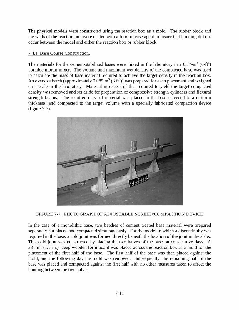
The physical models were constructed using the reaction box as a mold. The rubber block and the walls of the reaction box were coated with a form release agent to insure that bonding did not occur between the model and either the reaction box or rubber block.
7.4.1 Base Course Construction.
The materials for the cement-stabilized bases were mixed in the laboratory in a 0.17-m3 (6-ft3) portable mortar mixer. The volume and maximum wet density of the compacted base was used to calculate the mass of base material required to achieve the target density in the reaction box. An oversize batch (approximately 0.085 m3 (3 ft3)) was prepared for each placement and weighed on a scale in the laboratory. Material in excess of that required to yield the target compacted density was removed and set aside for preparation of compressive strength cylinders and flexural strength beams. The required mass of material was placed in the box, screeded to a uniform thickness, and compacted to the target volume with a specially fabricated compaction device (figure 7-7).
FIGURE 7-7. PHOTOGRAPH OF ADJUSTABLE SCREED/COMPACTION DEVICE
In the case of a monolithic base, two batches of cement treated base material were prepared separately but placed and compacted simultaneously. For the model in which a discontinuity was required in the base, a cold joint was formed directly beneath the location of the joint in the slabs. This cold joint was constructed by placing the two halves of the base on consecutive days. A 38-mm (1.5-in.) -deep wooden form board was placed across the reaction box as a mold for the placement of the fi rst half of the base. The first half of the base was then placed against the mold, and the following day the mold was removed. Subsequently, the remaining half of the base was placed and compacted against the first half with no other measures taken to affect the bonding between the two halves.
7-11

Three 51-mm (2-in.) -diameter by 102-mm (4-in.) -high cylinders were prepared from each batch of cement-treated base. The cylinders were prepared by compacting the base material into heavy, brass molds with a small, hand-held tamper. Also, three 76-mm (3-in.) -wide by 76-mm (3-in.) -deep by 286-mm (11-1/4-in.) -long beams were prepared from one batch of cement-treated base per model. The base material was compacted into steel molds using a hand-held tamper with a square footprint. These cylinders and beams were cured under the same conditions as the models and were tested on the date the corresponding experiment was conducted to determine the compressive strength, flexural strength, and modulus of elasticity of the cement-treated base.
The bond breaker for Experiment LSM-5 was constructed of two layers of 0.152-mm (6-mil) polyethylene sheets separated by a thin layer of uniformly graded fine silica sand. Prior to casting the concrete slabs, the first sheet of polyethylene was carefully cut and fitted on top of the base, as shown in the photograph in figure 7-8. Next, as fine a layer of the uniform sand as possible was spread on top of the polyethylene sheet (figure 7-9), and a second sheet, covering the entire surface, was placed on top of the sand layer. Then, the slabs were placed on top of the bond-breaking layer. Figure 7-10 is a photograph of the reaction box just prior to placement of the loaded slab.
Experiment LSM-6 featured an unbound granular base. The unbound base was placed in four lifts of approximately 25 mm (1 in.). The colors of the lifts were alternated between the natural color of the sand-silica blend and black. The black material was manufactured by mixing a black dye with the sand-silica blend during batching. Each lift was batched and mixed in a large Hobart paddle-type dough mixer. The mass required to achieve the targeted wet density was weighed out and placed in the reaction box. With the compaction device set to yield the required volume of compacted base, the material was compacted uniformly to yield the target wet density.
FIGURE 7-8. INSTALLATION OF POLYETHYLENE FILM IN REACTION BOX
7-12

FIGURE 7-9. PLACEMENT OF THIN SAND LAYER
FIGURE 7-10. BOND BREAKER AND DOWELED JOINT JUST PRIOR TO CONCRETE PLACEMENT
7.4.2 Slab Construction.
The two concrete slabs for each experiment were placed on consecutive days. The first slab was placed against a 51-mm (2-in.) -deep wooden mold faced with a 1.59-mm (1/16-in.) -thick sheet of Teflon. The dowels were inserted in 6-mm (0.25-in.) -diameter holes which had been predrilled through the mold and Teflon. Prior to their placement in the mold, a light coating of rust scale was removed from the dowels. The position of the dowels in the mold was adjusted to insure that equal lengths of dowel bars would be present in both slabs. A clamping device,
7-13

composed of pieces of wood cut to the proper dimensions and held together with screws, was used to insure that the dowels were held orthogonal to the mold. The bonded end of the dowel was placed in the fi rst slab; therefore, care was taken to insure that no form release agent, grease, or oil was present on the dowels.
The concrete was batched and mixed in the laboratory, carefully placed in the reaction box, and consolidated with an external spud-type concrete vibrator. The surface was floated and finished by hand, and the concrete was allowed to set for approximately 24 hours.
After 24 hours the transverse mold along the joint was carefully removed. The free ends of the dowels (unbonded ends) were greased with an automotive-type grease. To further insure that no bond could be developed between the dowel bars and the slab, plastic drinking straws with an inside diameter of 6 mm (0.25 in.) were slipped over the greased dowels. The second slab was then placed, consolidated, and finished.
The ends of the slabs were constrained by 76-mm (3-in.) equal leg structural steel angles, 9.5 mm (3/8 in.) thick. One leg of the angle was embedded in the fresh concrete just after placement, and the other leg was bolted to the side of the reaction box with 12.7-mm (0.5-in.) -diameter steel bolts. The bolts were later torqued to near yield to maximize the clamping force on the angles.
The slabs were moist cured using wet burlap and plastic sheeting at room temperature until they were placed in the environmental chamber at 60°C (140°F) over the weekend for accelerated curing. After they were removed from the environmental chamber, the slabs were allowed to cool in the laboratory to room temperature with no additional wet curing.
Three 152-mm (6-in.) -diameter by 305-mm (12-in.) -high cylinders were cast from each batch of concrete used to fabricate the model slabs. Also, a single 152-mm (6-in.) -wide by 152-mm (6-in.) -deep by 508-mm (20-in.) -long beam was cast from one batch of concrete for each model. These cylinders and beam were cured under the same accelerated curing conditions as the model slabs and were tested on the date the corresponding experiment was conducted to determine the compressive and flexural strengths, modulus of elasticity, and Poisson’s ratio of the slabs.
7.5 LOADING.
All experiments were conducted on the structural test floor at the Concrete Technology Division, Structures Laboratory, Waterways Experiment Station. Loads were applied to the physical model by a closed-loop, servo-hydraulic materials testing system through a thin, circular rubber pad. The radius of the loaded area, a, was 57 mm (2 1/4 in.). The testing system was controlled by an MTS LoadStar digital controller which could be programmed through a graphical user interface to output the desired control signals to the system. So that post-peak response could be captured, the load was applied in displacement control at a rate of 0.25 mm/min (0.01 in/min).
The testing frame consisted of four vertical steel columns bolted to attachment points in the structural test floor. A stiff, deep steel beam spanned the opening between the columns.
7-14

A 222-kN (50,000-lbs) capacity actuator attached to this beam provided the loading for the experiment.
7.6 INSTRUMENTATION.
Instrumentation for the physical model experiments consisted of the following:
a. Applied load measured by a load cell. b. Surface strains measured by surface-applied foil resistance strain gages. c. Displacement measured by linear variable displacement transducers (LVDT’s).
Al l strain and deformation measurements were made on the top surface of the slabs. The load cell was located between the testing machine actuator and the slab. The maximum range of the load cell was ±222 kN (50,000 lb).
Strain gages employed for these experimental studies had an electrical resistance of 350 ohms and a gage length of 25 mm (1 in.). When the gage was strained, it experienced a change in electrical resistance. These very small changes in resistance were measured by placing the gage in one leg of a Wheatstone bridge circuit, which is sensitive to small resistance changes. The maximum range of the strain gages was ±50,000 microstrains.
The locations for the strain gages were prepared by first applying a thin coat of Epicast, a low-modulus, white epoxy. This epoxy coat served two primary functions: to provide a moisture barrier to prevent water in the concrete from affecting the strain gage and to provide a smooth, uniform surface to which the strain gage could be bonded. After a 24-hour setting period, the Epicast was sanded to a uniform thickness, and the strain gages were bonded using Super Glue.
The LVDT is a transformer-type device that translates straight-line mechanical motion into an alternating current (AC) analog voltage. Each LVDT contained a movable magnetic core which rested on the surface of the concrete. As the surface of the concrete was displaced, the movement of the core caused an electromagnetic imbalance in the transformer, which in turn, output a proportional AC voltage. As calibrated for these experiments, the maximum range of the LVDT’s was approximately 2.5 mm (0.1 in). All L VDT’s were mounted to one or more steel angles which spanned the reaction box. The ends of these angles were rigidly attached to the reaction box using machine screws.
All data from these instruments were acquired in real time using a MEGADAC data acquisition system manufactured by Optim Electronics Corporation of Germantown, Maryland. The MEGADAC system is programmed and controlled by a Pentium personal computer running Optim’s Test Control Software, which converts the analog signals to digital data using the appropriate gage calibration factors and saves the digital data to disk.
A Kodak DC 40 digital still-image camera was positioned approximately 200 mm (8 in.) from the transparent window on the side of the box. This camera was set to record digital images of the slab-joint-base region.
7-15

7.7 EXPERIMENTAL RESULTS.
Experiments LSM-1 through LSM-6 were conducted during the period from March 27, 1996, to June 5, 1996. However, Experiment LSM-3 was not considered to be a valid test due to problems encountered during the conduct of the experiment. An error was made in programming the loading function into the MTS TestStar controller, and the loading was not carried out as planned. Therefore, the results from LSM-3 were thrown out, and a repeat of the experiment (LSM-3R) was conducted on June 19, 1996. The results of quality control tests conducted on the construction materials as well as data from each of the experiments is presented and discussed in this section.
7.8 MATERIALS.
7.8.1 Cement-Stabilized Bases.
The results of the quality control tests on the cement-stabilized bases are summarized in table 7-5. Each numerical value reported in the table represents the mean of three replicates. Compressive strength tests were conducted on 51-mm (2-in.) by 102-mm (4-in.) cylindrical specimens. The compressive strengths of the stabilized bases were at or below that expected from the 7-day accelerated curing tests conducted during the initial materials investigation (figure 7-4). It is believed that the lower strengths can be attributed to drying out of the cement/silty-sand material between batching and preparation of the test specimens. The material to be used to make the specimens was set aside while the bases were placed and compacted in the reaction box. Typically, more than 1 but less than 2 hours elapsed between the batching of the base materials and preparation of the quality control specimens. It is likely that some of the moisture evaporated during this period, resulting in lower densities and strengths in the quality control specimens.
TABLE 7-5. RESULTS OF QUALITY CONTROL TESTS ON CEMENT-STABILIZ ED BASE
Experiment Location
Compression Tests Flexural Tests
Replicates
Compressive Strength
MPa (psi)
Modulus of Elasticity
MPa (106 psi) Flexural Strength
MPa (psi)
Mean Std. Dev. Mean
Std. Dev. Replicates Mean
Std. Dev.
LSM-3R Top Li ft 3
6.59 (826)
1.35 (196)
1,520 (0.220)
662 (0.096) 3
1.23 (179)
0.05 (8)
Bottom Li ft 3
6.24 (904)
0.48 (69)
1,822 (0.264)
693 (0.100) No Tests Conducted
LSM-4 Right Half 3
4.50 (653)
0.51 (73)
1,220 (0.177)
645 (0.093) 3
1.18 (171)
0.04 (5)
Left Half 3
4.49 (652)
0.76 (110)
1,390 (0.202)
248 (0.036) No Tests Conducted
LSM-5 Top Li ft 3
5.92 (858)
0.29 (41)
1,440 (0.208)
395 (0.057) 3
1.20 (174)
0.05 (8)
Bottom Li ft 3
4.45 (645)
0.99 (144)
1,070 (0.155)
383 (0.056) No Tests Conducted
7-16

The modulus of elasticity of the cement-stabilized base was determined from the compressive strength tests on the cylinders. The modulus of elasticity (in compression), as calculated from the tangent to the steepest portion of the compressive stress-strain curve, is tabulated in table 7-5. These data indicate that as the compressive strength increases, the compressive modulus of elasticity increases. The modulus of elasticity of the cement-stabilized base was approximately 5 percent of the target modulus of elasticity of the Portland cement concrete slabs.
The modulus of rupture (flexural strength) of the cement-stabilized base was determined from tests on 76-mm (3-in.) by 76-mm (3-in.) by 286-mm (11 1/4-in.) beams loaded at the third points. These data are also reported in table 7-5.
Statistical techniques were employed to determine if the observed variations in the material properties from batch to batch within an experiment and between experiments were statistically significant at the 0.05 significance level. Student’s t-tests were conducted on the compressive strength and modulus of elasticity data from the two batches of cement-stabilized base material within each experiment. For each of the Experiments LSM-3R, LSM-4, and LSM-5, the differences in the mean values of compressive strength and modulus of elasticity between batches were not great enough to exclude the possibility that the differences were due to random sampling variability.
Therefore, it can be concluded that there was no statistically significant difference in compressive strength and elastic modulus between batches in any given experiment at the 0.05 significance level.
One-way analysis of the variance (ANOVA) procedures were used to test for statistically significant differences in material properties between experiments. The results of these analyses indicated that for the case of compressive strength, the differences in the mean values of compressive strength between experiments were greater than would be expected by chance at the 0.05 significance level. A pairwise multiple comparison test indicated that the compressive strength values from Experiment LSM-3R were statistically different from those of LSM-4 and LSM-5. However, for the cases of modulus of elasticity and flexural strength, the differences in the mean values between experiments were not great enough to exclude the possibility that the difference was due to random sampling variability; therefore, no statistically significant differences in these two parameters were detected at the 0.05 significance level.
7.8.2 Portland Cement Concrete.
The properties of the fresh Portland cement concrete used to construct the slabs for the laboratory-scale model experiments are tabulated in table 7-6. Tests conducted on the fresh concrete included slump (per ASTM C 143-90a) and unit weight (per ASTM C 131-92). The theoretical air content was calculated from the measured unit weight. The results of tests on hardened concrete cylinders and beams are reported in table 7-7. Tests on 152-mm (6-in.) by 305-mm (12-in.) concrete cylinders included compressive strength (per ASTM C 39-93) and modulus of elasticity and Poisson’s ratio (per ASTM C 469-94). Flexural strength (modulus of rupture) tests were conducted on 152-mm (6-in.) by 152-mm (6-in.) by 305-mm (12-in.)
7-17

prismatic beams loaded as the third points per ASTM C 78-94. As noted in table 7-7, all hardened concrete tests results for Experiment LSM-2 were lost due to failure of the concrete testing machine on the day of the tests.
TABLE 7-6. RESULTS OF TESTS ON FRESH PORTLAND CEMENT CONCRETE
Experiment Casting
Date
Batch Placement Location
Slump mm (in.)
Unit Weight kg/m3 (pcf)
Air Content Percent
LSM-1 3/20/96 Left Slab 70 (2¾) 2,268 (141.6) 1.8
3/21/96 Right Slab 51 (2) 2,243 (140.0) 2.8
LSM-2 4/3/96 Left Slab 70 (2¾) 2,236 (139.6) 3.1
4/4/96 Right Slab 64 (2½) 2,230 (139.2) 3.5
LSM-3R 6/12/96 Left Slab 51 (2) 2,252 (140.6) 2.5
6/13/96 Right Slab 64 (2½) 2,243 (140.0) 2.8
LSM-4 5/1/96 Left Slab 70 (2¾) 2,256 (140.8) 2.3
5/2/96 Right Slab 102 (4) 2,246 (140.2) 2.7
LSM-5 5/14/96 Left Slab 76 (3) 2,236 (139.6) 3.2
5/16/96 Right Slab 127 (5) 2,217 (138.4) 4.0
LSM-6 5/29/96 Left Slab 127 (5) 2,243 (140.0) 2.8
5/30/96 Right Slab 152 (6) 2,236 (139.6) 3.1
The slump of the fresh concrete varied from 51 mm ( 2 in.) to 127 mm (5 in.), with the majority of the measurements between 51 mm (2 in.) and 76 mm (3 in.). Models LSM-1, LSM-2, and the left slab of LSM-4 were all fabricated from the same lot of Type III cement, while models LSM-3R, LSM-5, LSM-6, and the right slab of LSM-4 were fabricated from a different lot of Type III cement from the same manufacturer. The higher slump values noted for models LSM-4 (right slab), LSM-5, and LSM-6 were attributed to the changes in the cement between the two lots. The second lot had less water demand than the first resulting in an increase in the slump of the fresh concrete. This effect was mitigated for Experiment LSM-3R by reducing the mix water by 6 percent (by mass) thus bringing the slump back in line with the models fabricated from the first lot of cement. Unit weights of the fresh concrete varied from 2,217 kg/m3 (138.4 pcf) to 2,268 kg/m3 (141.6 pcf), while air contents ranged from 1.8 to 4.0 percent.
The mean concrete compressive strengths ranged from a low of 25.6 MPa (3,710 psi) to a high of 29.0 MPa (4,200 psi). The modulus of elasticity ranged from 26,800 MPa (3.9 × 10⁶ psi) to 29,000 psi (4.2 × 10⁶ psi), while Poission’s ratio ranged from 0.17 to 0.19. The modulus of rupture varied from a minimum of 2.90 MPa (420 psi) to a maximum of 3.28 MPa (475 psi).
7-18

7-19
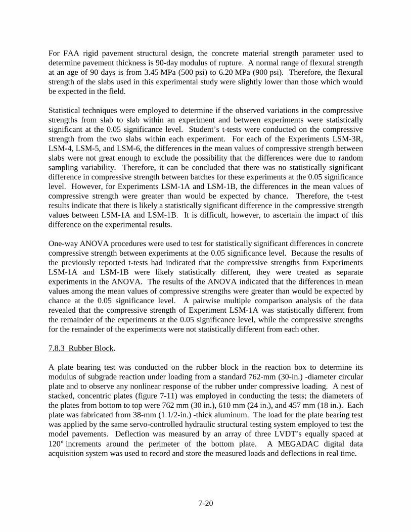
For FAA rigid pavement structural design, the concrete material strength parameter used to determine pavement thickness is 90-day modulus of rupture. A normal range of flexural strength at an age of 90 days is from 3.45 MPa (500 psi) to 6.20 MPa (900 psi). Therefore, the flexural strength of the slabs used in this experimental study were slightly lower than those which would be expected in the field.
Statistical techniques were employed to determine if the observed variations in the compressive strengths from slab to slab within an experiment and between experiments were statistically significant at the 0.05 significance level. Student’s t-tests were conducted on the compressive strength from the two slabs within each experiment. For each of the Experiments LSM-3R, LSM-4, LSM-5, and LSM-6, the differences in the mean values of compressive strength between slabs were not great enough to exclude the possibility that the differences were due to random sampling variability. Therefore, it can be concluded that there was no statistically significant difference in compressive strength between batches for these experiments at the 0.05 significance level. However, for Experiments LSM-1A and LSM-1B, the differences in the mean values of compressive strength were greater than would be expected by chance. Therefore, the t-test results indicate that there is likely a statistically significant difference in the compressive strength values between LSM-1A and LSM-1B. It is difficult, however, to ascertain the impact of this difference on the experimental results.
One-way ANOVA procedures were used to test for statistically significant differences in concrete compressive strength between experiments at the 0.05 significance level. Because the results of the previously reported t-tests had indicated that the compressive strengths from Experiments LSM-1A and LSM-1B were likely statistically different, they were treated as separate experiments in the ANOVA. The results of the ANOVA indicated that the differences in mean values among the mean values of compressive strengths were greater than would be expected by chance at the 0.05 significance level. A pairwise multiple comparison analysis of the data revealed that the compressive strength of Experiment LSM-1A was statistically different from the remainder of the experiments at the 0.05 significance level, while the compressive strengths for the remainder of the experiments were not statistically different from each other.
7.8.3 Rubber Block.
A plate bearing test was conducted on the rubber block in the reaction box to determine its modulus of subgrade reaction under loading from a standard 762-mm (30-in.) -diameter circular plate and to observe any nonlinear response of the rubber under compressive loading. A nest of stacked, concentric plates (figure 7-11) was employed in conducting the tests; the diameters of the plates from bottom to top were 762 mm (30 in.), 610 mm (24 in.), and 457 mm (18 in.). Each plate was fabricated from 38-mm (1 1/2-in.) -thick aluminum. The load for the plate bearing test was applied by the same servo-controlled hydraulic structural testing system employed to test the model pavements. Deflection was measured by an array of three LVDT’s equally spaced at 120° increments around the perimeter of the bottom plate. A MEGADAC digital data acquisition system was used to record and store the measured loads and deflections in real time.
7-20

FIGURE 7-11. TEST SETUP FOR PLATE BEARING TEST ON RUBBER PAD
Two loading regimes were followed for this testing. The first was conducted in load control following the applicable procedures specified in Section XII, FM 5-530 (Department of the Army, 1987). A seating load of 6.8 kPa (1 psi) was applied to the plate. This was considered to be the zero point of the test. An additional load increment was then applied to bring the plate bearing stress to 68.9 kPa (10 psi), where the load was held for several minutes until the rate of deformation was less than 0.005 mm/min (0.0002 in./min). Subsequently, an additional increment of load was applied to bring the plate bearing stress to 103 kPa (15 psi), where the load was again held until the rate of deformation was less than 0.005 mm/min (0.0002 in./min). This procedure was repeated at increments of plate bearing stress of 34.4 kPa (5 psi) up to a maximum stress of 207 kPa (30 psi). Finally, the load was decreased slowly until the applied stress was zero. A plot of plate bearing stress versus plate displacement is presented in figure 7-12. It is apparent from this plot that the rubber pad crept during the portions of the tests where the plate bearing stress was held constant. It can also be seen that the amount of creep deformation which occurs until the rate of creep deformation falls below 0.005 mm/min (0.0002 in./min) increases with increasing plate bearing stress. The accumulated creep deformation at the end of the loading was approximately 0.4 mm (0.016 in.).
The data from this test were used to determine the modulus of subgrade reaction, k, for the rubber block for the standard 762-mm (30-in.) -diameter plate. Figure 7-13 shows a plot of corrected plate bearing stress versus displacement as prescribed by FM 5-530 (Department of the Army, 1987). Each of the data points denoted by the filled triangles represents the deflection and stress at the end of each increment of applied stress, adjusted for the 6.8 kPa (1 psi) initial seating load. These data were then corrected, using the procedures described in FM 5-530 (Department of the Army 1987), to account for bending of the plates. From the slope of the corrected curve, the modulus of subgrade reaction was determined to be 111 MPa/m (409 psi/in.). This value is high for a subgrade material and would be more representative of the modulus of subgrade reaction for a dense, well-graded gravel.
7-21

Plate Bearing Test in Load Control (762-mm (30-in.) -Diameter Plate)
FIGURE 7-12. PLATE BEARING STRESS-DISPLACEMENT DATA FROM PLATE BEARING TEST ON RUBBER BLOCK IN LOAD CONTROL
762-mm (30-in.) -Diameter Plate
FIGURE 7-13. CORRECTED PLATE BEARING STRESS
The second loading regime was conducted in displacement control at a load rate of 0.25 mm/min (0.01 in./min) to mimic the loading conditions during testing of a pavement model. The bearing
7-22

plate was displaced continuously and monotonically until a maximum bearing stress of 0.1 MPa (14.5 psi) was reached, at which point the displacement was reversed continuously and monotonically until the bearing stress was reduced to zero. A plot of bearing stress versus deformation is shown in figure 7-14. In the range in which the bearing stress was less than 0.01 MPa (1.5 psi), the response was relatively soft. For bearing stresses greater than approximately 0.1 MPa (1.5 psi) the response was stiffer. Upon unloading, the response was characterized by a hysterisis loop typical of visco-elastic materials. Thus, it can be concluded that the response of the rubber block in the reaction box was nonlinear visco-elastic over the range of loading expected during testing of a pavement model. These nonlinear responses of the rubber block are considerably different from those assumed for the bed-of-springs foundation in Westergaard’s theory. The influence of the nonlinear visco-elastic response on the pavement model is not known.
Plate Bearing Test in Displacement Control (762-mm (30-in.) -Diameter Plate)
FIGURE 7-14. PLATE BEARING STRESS-DISPLACEMENT DATA FROM PLATE BEARING TEST ON RUBBER BLOCK IN DISPLACEMENT CONTROL
7.9 EXPERIMENT LSM-1.
Experiment LSM-1 consisted of two 51-mm (2-in.) -thick slabs founded directly on the rubber subgrade. The right- and left-hand slabs were constructed with no load transfer capabilities from either dowel bars or aggregate interlock. A 5-mm (3/16-in.) gap separated the slabs to insure that no incidental contact could occur between the slabs during testing. The experiment consisted of two separate loadings: an edge loading near the center of the right-hand slab, referred to as LSM-1A, and a corner loading near the transparent window pane on the left-hand slab, referred to as LSM-1B. The results from both of these experiments are presented and discussed in this section.
7-23

7.9.1 Experiment LSM-1A.
The instrumentation locations for LSM-1A are presented in figure 7-15. The LVDT locations were selected to give two deflection basin profiles: one perpendicular to the free edge and one parallel to the free edge. The strain gage array was set to give only one strain profile perpendicular to the free edge.
FIGURE 7-15. INSTRUMENTATION PLAN, EXPERIMENT LSM-1A
Figure 7-16 is a plot of the load-time history of the test. The test was conducted by applying 10 preloading cycles of 1.78 kN (400 lb) triangular pulses. The purpose of these pulses was to “work” the model so that any potential restrictions to deformation that might be present as a result of the model construction would be overcome before actual loading began. These preloading cycles were followed by cycles of increasing loading intensity until the testing was stopped. This included the application of four additional cycles of loading until the test was stopped at a maximum load of approximately 26 kN (5,850 lbs).
7-24

FIGURE 7-16. LOADING HISTORY, EXPERIMENT LSM-1A
Figure 7-17 is a posttest photograph of the slabs after both Experiments LSM-1A and LSM-1B. Failure of the slab in Experiment LSM-1A, loaded near the edge, was characterized by a semi-circular crack labeled LSM-1A in the photograph. This cracking pattern is not typical of those observed in airport pavement condition surveys. Visible cracks were first observed with the naked eye at a load of approximately 17.3 kN (3,900 lb).
FIGURE 7-17. POSTTEST PHOTOGRAPH, EXPERIMENTS LSM-1A AND LSM-1B
Data traces from the LVDT’s on the surface of the slab are contained in appendix B. The traces from the ten preloading cycles have been removed for clarity. For all LVDT measurements, a downward displacement is considered to be positive, while an upward movement is negative. Gage D4 overranged at a displacement of approximately 2.5 mm (0.1 in.). One obvious
7-25

observation is that the overall shape of the load-displacement curves was similar to that recorded during the plate bearing test in displacement control. The slope of the curves changed at a load of approximately 5 kN (1,125 lb), as was observed in the plate bearing tests. Therefore, it was concluded that this change in stiffness can be attributed to the rubber block foundation and not to the Portland cement concrete slab. Hysteresis loops and the attendant viscous deformations can be seen with each unloading cycle.
Data traces from the strain gages on the surface of the slab are found in appendix B. For strain gage measurements, tensile strains are positive, and compressive strains are negative. The strains are compressive at loads less than approximately 7 kN (1,575 lb). Beyond first cracking, the gages nearest the edge of the slab (S4 and S3) reverse directions and go into the tensile regime possibly indicating localized cracking.
In order to compare the data from this experiment with linear elastic calculations made with a finite element code, it was desirable to correct the load-displacement data to remove the nonlinear response of the rubber block. A technique similar to that used to correct for nonlinear response in the plate bearing test was used to perform this correction. Figures 7-18 and 7-19 show the raw and corrected load-displacement curves for the third cycle of loading for the LVDT’s along a line perpendicular and parallel to the edge, respectively. The slopes of the linear portions of the load-deflection curves (that portion of the curve above approximately 5 kN (1,125 lb)) were determined numerically. The load-deflection curves were then shifted right such that the extension of the linear portion of the curve would pass through the origin as shown in figures 7-18 and 7-19.
FIGURE 7-18. RAW AND CORRECTED DISPLACEMENT DATA FROM LVDT’S POSITIONED PERPENDICULAR TO EDGE, EXPERIMENT LSM-1A
7-26

FIGURE 7-19. RAW AND CORRECTED DISPLACEMENT DATA FROM LVDT’S POSITIONED PARALLEL TO EDGE, EXPERIMENT LSM-1A
Deflection basins from the corrected load-deflection curves were then compared with linear elastic finite element calculations made with ABAQUS using the S8R5 reduced integration, second-order shell element. Initial calculations were made with the foundation modulus of subgrade reaction set at k = 27, 54, 82, and 109 MPa/m (100, 200, 300, and 400 psi/in.). The ABAQUS deflection profiles at points identical to the locations of the LVDT’s along lines parallel and perpendicular to the edge were compared with the experimental deflection basin profiles.
Figure 7-20 shows a log-log plot obtained analytically of the modulus of subgrade reaction versus deflection (w) at gage location D4 for a load of 6 kN (1,350 lb) from the ABAQUS finite element calculations. This magnitude of load was chosen because it is midway between the value at which the change in slope occurs in the response of the rubber foundation at 5 kN (1,125 lb) and the load at which the onset of possible cracking occurred at 7 kN (1,575 lb). Upon entering this plot with the experimental deflection obtained from gage D4 at P = 6 kN (1,350 lb), the value of k for the edge loading case can be estimated as about 70 MPa/m (258 psi/in.). An additional ABAQUS calculation was made using this value of k. The deflection basin profiles along the lines of LVDT’s are shown in figures 7-21 and 7-22. These figures show excellent agreement between the ABAQUS runs and experiment at the location of gage D4. However, the agreement deteriorates for gages distant from D4, particularly for the basin perpendicular to the edge. This disagreement was expected, because it is well known that backcalculated values of k vary as one moves away from the edge of a rigid pavement slab.
The backcalculated modulus of subgrade reaction for the rubber block in the reaction box differs significantly from that obtained from the plate bearing test. Again, this was not surprising, because it has been known at least since the 1940’s that modulus of subgrade reaction is not an intrinsic material property, but rather the value of k is dependent upon the conditions of the test run to estimate it.
7-27

FIGURE 7-20. ANAL YTICAL RELATIONSHIP BETWEEN MODULUS OF SUBGRADE REACTION AND DEFLECTION FROM ABAQUS MODELS, EXPERIMENT LSM-1A
Distance From Joint, mm
FIGURE 7-21. COMPARISON OF EXPERIMENTAL AND ANAL YTICAL DEFLECTION BASIN PROFILES PERPENDICULAR TO EDGE, EXPERIMENT LSM-1A
7-28

Distance From Front of Slab, mm
FIGURE 7-22. COMPARISON OF EXPERIMENTAL AND ANAL YTICAL DEFLECTION BASIN PROFILES PARALLEL TO EDGE, EXPERIMENT LSM-1A
7.9.2 Experiment LSM-1B.
The instrument locations for test LSM-1B are indicated in figure 7-23. A single array of LVDT’s were placed along a line perpendicular to the free of the left-hand slab near the loaded area. Similarly, a line of foil strain gages were placed on the surface of the left-hand slab along a line perpendicular to the edge. The left-hand slab in figure 7-17 shows the cracking patterns observed after the test was completed. Visible cracking was first observed with the unaided eye at a load of approximately 16.9 kN (3,800 lb).
The loading plan followed in Experiment LSM-1B was identical to that followed in Experiment LSM-1A. Figure 7-24 shows the loading history for Experiment LSM-1B. A brief power outage lasting a few seconds occurred during the 10 preloading cycles. The MTS LoadStar control system and MEGADAC data acquisition systems were powered by uninterruptible power supplies during the power outage and thus were not affected. However, the hydraulic system of the loader was briefly without power, and the load dropped off until power was restored. At this point the control system reassumed control of the loader, and the test was continued.
The load-deflection traces from the LVDT’s are presented in appendix B. The trends observed in these traces are similar to those discussed for Experiment LSM-1A.
7-29

FIGURE 7-23. INSTRUMENTATION PLAN, EXPERIMENT LSM-1B
FIGURE 7-24. LOADING HISTORY, EXPERIMENT LSM-1B
7-30

The plots from the strain gages are also presented in appendix B. These data traces show that the strain gages on the top surface of the slab registered tensile strains. Even though the crack passed close to Gage S1, cracking cannot be discerned in the strain gage traces.
The load-deflection curves from LSM-1B were corrected for the nonlinear response of the rubber foundation in the manner described for Experiment LSM-1A. The shifted raw data traces along with the corrected data are presented in figure 7-25. Deflection basins from the corrected load-deflection curves were then compared with linear elastic finite element calculations made with ABAQUS using the S8R5 reduced integration, second-order shell elements. Again, initial calculations were made with the modulus of subgrade reaction set at k = 27, 54, 82, and 109 MPa/m (100, 200, 300, and 400 psi/in.). The ABAQUS deflection profiles at points identical to the locations of the LVDT’s were compared with the experimental deflection basin profile.
FIGURE 7-25. RAW AND CORRECTED DISPLACEMNT DATA FROM LVDT’S, EXPERIMENT LSM-1B
Figure 7-26 shows a log-log plot obtained analytically of the modulus of subgrade reaction versus deflection (w) at gage location D4 for a load of 6.1 kN (1,370 lb) from the ABAQUS finite element calculations. Entering this plot with the experimental deflection obtained from gage D4 at P = 6.1 kN (1,370 lb), the value of k can be estimated as about 90 MPa/m (330 psi/in.). An additional ABAQUS calculation was made using this value of k. The deflection basin profiles along the line of LVDT’s are shown in figure 7-27. As was the case for Experiment LSM-1A, excellent agreement between the ABAQUS runs and experiment at the location of gage D4 was obtained.
7-31
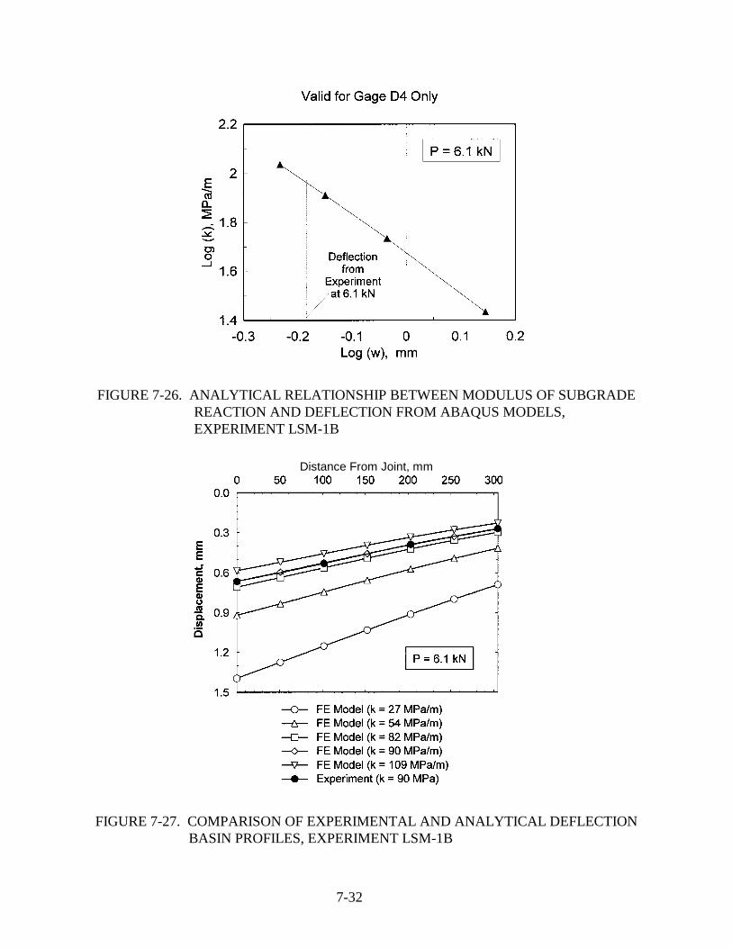
FIGURE 7-26. ANAL YTICAL RELATIONSHIP BETWEEN MODULUS OF SUBGRADE REACTION AND DEFLECTION FROM ABAQUS MODELS, EXPERIMENT LSM-1B
Distance From Joint, mm
FIGURE 7-27. COMPARISON OF EXPERIMENTAL AND ANAL YTICAL DEFLECTION BASIN PROFILES, EXPERIMENT LSM-1B
7-32
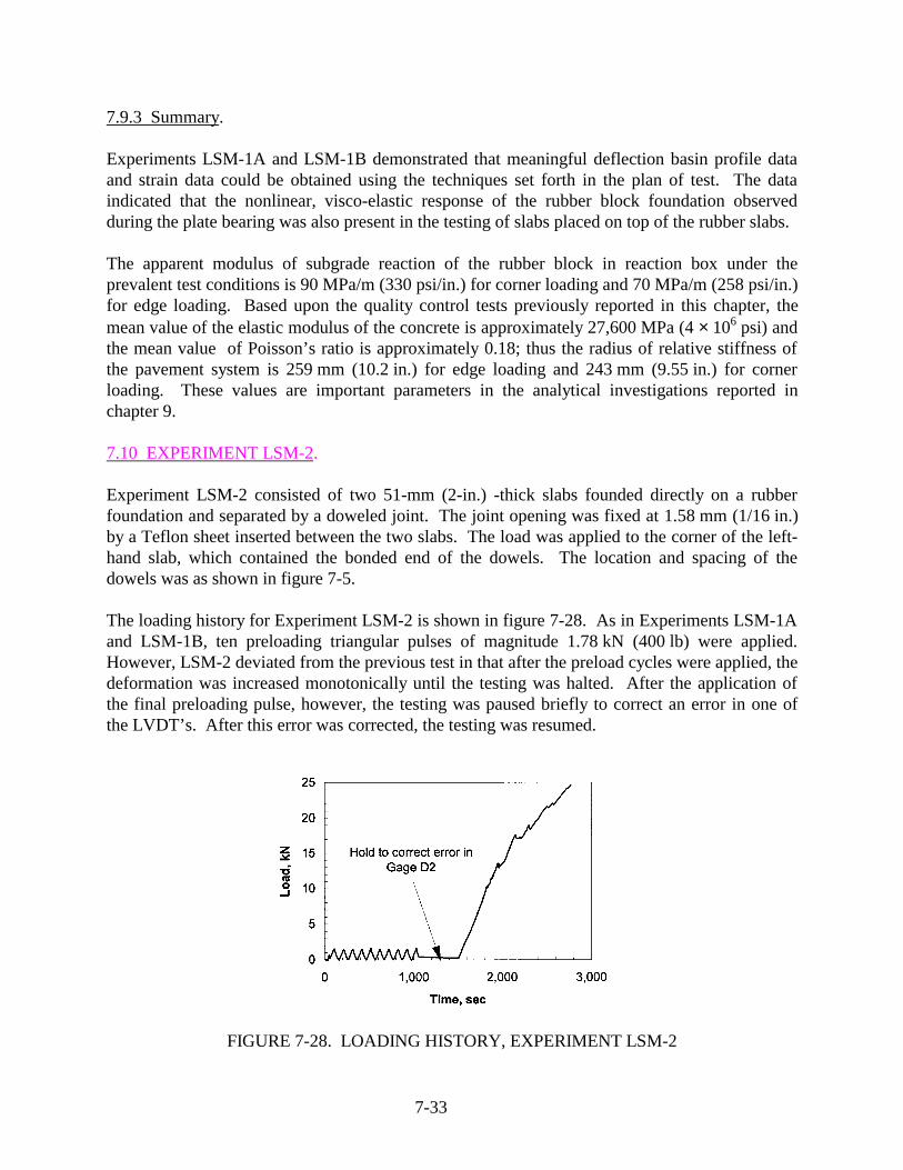
7.9.3 Summary.
Experiments LSM-1A and LSM-1B demonstrated that meaningful deflection basin profile data and strain data could be obtained using the techniques set forth in the plan of test. The data indicated that the nonlinear, visco-elastic response of the rubber block foundation observed during the plate bearing was also present in the testing of slabs placed on top of the rubber slabs.
The apparent modulus of subgrade reaction of the rubber block in reaction box under the prevalent test conditions is 90 MPa/m (330 psi/in.) for corner loading and 70 MPa/m (258 psi/in.) for edge loading. Based upon the quality control tests previously reported in this chapter, the mean value of the elastic modulus of the concrete is approximately 27,600 MPa (4 × 10⁶ psi) and the mean value of Poisson’s ratio is approximately 0.18; thus the radius of relative stiffness of the pavement system is 259 mm (10.2 in.) for edge loading and 243 mm (9.55 in.) for corner loading. These values are important parameters in the analytical investigations reported in chapter 9.
7.10 EXPERIMENT LSM-2.
Experiment LSM-2 consisted of two 51-mm (2-in.) -thick slabs founded directly on a rubber foundation and separated by a doweled joint. The joint opening was fixed at 1.58 mm (1/16 in.) by a Teflon sheet inserted between the two slabs. The load was applied to the corner of the left-hand slab, which contained the bonded end of the dowels. The location and spacing of the dowels was as shown in figure 7-5.
The loading history for Experiment LSM-2 is shown in figure 7-28. As in Experiments LSM-1A and LSM-1B, ten preloading triangular pulses of magnitude 1.78 kN (400 lb) were applied. However, LSM-2 deviated from the previous test in that after the preload cycles were applied, the deformation was increased monotonically until the testing was halted. After the application of the final preloading pulse, however, the testing was paused briefly to correct an error in one of the LVDT’s. After this error was corrected, the testing was resumed.
FIGURE 7-28. LOADING HISTORY, EXPERIMENT LSM-2
7-33

The instrumentation plan for Experiment LSM-2 is presented in figure 7-29. This is the instrumentation plan which would be adhered to for the remainder of the experimental program. A line of LVDT’s spanned across the joint to capture the deflection basin profile. Also, a line of strain gages were placed on the top surface of the slabs.
FIGURE 7-29. INSTRUMENTATION PLAN, EXPERIMENTS LSM-2, -3R, -4, -5, AND -6
A posttest photograph of the top surface of the slabs is shown in figure 7-30. The cracking highlighted on the left (loaded) slab was first observed at a load of approximately 17 kN (3,800 lb), while the cracking on the unloaded side was first observed at a load of approximately 19.1 kN (4,300 lb). A series of three photographs taken through the transparent window in the side of the reaction box is shown in figure 7-31. The faint grids in the foreground of the photographs are spaced at 12.7 mm (1/2 in.). As the load is increased from zero to 13.3 kN (3,000 lb), the deflection of the top surface of the slabs is evident. Also note that no visible cracking can be noted in the sides of the slabs at 13.3 kN (3,000 lb). However, by the time the load had increased to 17.8 kN (4,000 lb), a vertical crack was clearly visible directly beneath the loaded area in the left slab. Also, a crack which runs more or less horizontally from the joint is visible in the right (unloaded) slab. A posttest examination of the crack revealed that it originated at the dowel directly opposite the center of the loaded area and ran out and down toward the edge and base of the right slab.
7-34

FIGURE 7-30. POSTTEST PHOTOGRAPH OF SLAB TO SURFACE, EXPERIMENT LSM-2
FIGURE 7-31. SERIES OF PHOTOGRAPHS IN VICINITY OF JOINT, EXPERIMENT LSM-2
The load-displacement traces from the array of LVDT’s are presented in appendix B. As noted in the figure, Gage D4 was overranged at a load of approximately 23 kN (5,000 lb). These traces indicate clear evidence of cracking at loads greater than approximately 10 kN (2,350 lb). Selected deflection basin profiles are plotted in figure 7-32. Highly nonlinear response indicating severe cracking near the loaded area is evident for the deflection basins at 20 kN (4,500 lb) and 24 kN (5,500 lb).
The traces from the strain gages bonded to the surface of the slabs are found in appendix B. These data clearly show the formation of the cracking which is visible on the top surface of the slab: on the left (loaded) slab at approximately 17 kN (3,800 lb) and on the right (unloaded) slab at 19.1 kN (4,300 lb).
7-35

Distance From Joint, mm
FIGURE 7-32. SELECTED DEFLECTION BASIN PROFILES, EXPERIMENT LSM-2
7.11 EXPERIMENT LSM-3R.
Experiment LSM-3 was scrapped because of an operator error in programming the loading function into the MTS Test Star loader. Therefore, a second model was fabricated and tested with the designation of LSM-3R. The model consisted of two 51-mm (2-in.) -thick slabs (separated by a doweled joint) founded on a monolithic 38.1-mm (1 1/2-in.) -thick cement-stabilized base. The base was placed directly on the rubber block subgrade model. A Teflon sheet inserted between the two slabs maintained the joint opening at 1.58 mm (1/16 in.). A circular load was applied near the corner of the left-hand slab, which contained the bonded end of the dowels. The location and spacing of the dowels is shown in figure 7-5. Instrumentation type and locations for LSM-3R were identical to that for LSM-2 (figure 7-29).
The loading history for LSM-3R (figure 7-33) indicates that the load underwent several cycles of unloading and reloading near the peak load as cracks formed and the stresses were redistributed in the model. A transient reduction in stiffness of the pavement model was evident between approximately 12 kN (2,700 lb) and 16 kN (3,600 lb). Figure 7-34 is a posttest photograph of the top surface of the model. Several corner breaks are evident on the surface of the left-hand or loaded slab. The occurrence of the outermost corner break corresponded with the first peak in the loading history plot at approximately 38 kN (8,550 lb), while the inner break corresponded with the second major peak at approximately 37 kN (8,300 lb). Posttest observations indicated that these cracks in the slab propagated through the stabilized base as well. No debonding of the base from the slabs at their interface was observed. Considerable crushing or punching shear deformations were noted in and around the circular loaded area.
7-36
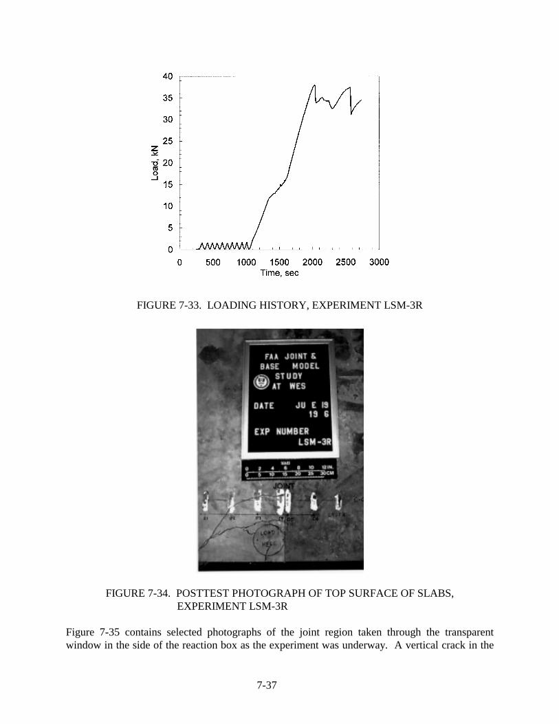
FIGURE 7-33. LOADING HISTORY, EXPERIMENT LSM-3R
FIGURE 7-34. POSTTEST PHOTOGRAPH OF TOP SURFACE OF SLABS, EXPERIMENT LSM-3R
Figure 7-35 contains selected photographs of the joint region taken through the transparent window in the side of the reaction box as the experiment was underway. A vertical crack in the
7-37

cement-stabilized base was clearly visible to the unaided eye at a load of 7.9 kN (2,000 lb). The lower left photograph was taken at a load of 37.8 kN (8,500 lb), which is near the first peak in the load-deflection curve. The lower right photograph was taken just prior to halting the test. Note that the vertical crack in the base has opened considerably, and horizontal cracking is evident in the left- and right-hand slabs and in the base underneath the right-hand slab.
FIGURE 7-35. SELECTED PHOTOGRAPHS OF JOINT REGION DURING TESTING, EXPERIMENT LSM-3R
The load-displacement and load-strain traces are presented in appendix B. The effects of the cracking which occurred near peak load are evident in these data. Selected deflection basin profiles are plotted in figure 7-36. Insight into the influence of the stabilized base course on the postcracking response of the slabs can be gained by comparing the deflection basin profiles in figure 7-36 with those from Experiment LSM-2 (figure 7-32). The basins from Experiment LSM-2 (with no base course) are highly nonlinear after cracking has occurred indicating the slab is breaking apart under increasing loads. However, for Experiment LSM-3R (with stabilized
7-38

base), the postcracking deflection basins do not indicate that the slab response is nearly as nonlinear as that observed in Experiment LSM-2.
Distance From Joint, mm
FIGURE 7-36. SELECTED DEFLECTION BASIN PROFILES, EXPERIMENT LSM-3R
7.12 EXPERIMENT LSM-4.
Two 51-mm (2-in.) -thick slabs (separated by a doweled joint) founded on a 37.1-mm (1 1/2-in.) -thick cement-stabilized base were constructed and tested for Experiment LSM-4. The base was divided into two equal halves by a cold-joint discontinuity directly beneath the slab construction joint. The base was founded directly on the rubber block subgrade model.
A Teflon sheet inserted between the two slabs maintained the slab joint opening at 1.58 mm (1/16 in.). A circular load was applied near the corner of the left-hand slab, which contained the bonded end of the dowels. The location and spacing of the dowels is shown in figure 7-5. Instrumentation type and locations for LSM-4 were identical to that for LSM-2 and LSM-3R (figure 7-29).
The loading history for LSM-4 (figure 7-37) is similar in form to that of LSM-3R. A transient reduction in stiffness of the pavement model occurred in the vicinity of a load of 15 kN (3,400 lb). Figure 7-38 is a posttest photograph of the top surface of the model. The cracking shown in the photograph occurred on both the loaded and unloaded sides of the joint and is nearly symmetrical about the joint. As was the case for Experiment LSM-3R, the cracking pattern in the slabs was reflected in the base course as well. Again, no debonding of the slab-base interface was observed.
7-39

FIGURE 7-37. LOADING HISTORY, EXPERIMENT LSM-4
FIGURE 7-38. POSTTEST PHOTOGRAPH OF TOP SURFACE OF SLABS, EXPERIMENT LSM-4
Figure 7-39 contains selected photographs of the joint region taken through the transparent window in the side of the reaction box during the experiment. Before the testing commenced,
7-40

the cold-joint discontinuity is visible in the base. As the deflection increased, the cold joint opened up.
Cold Joint
FIGURE 7-39. SELECTED PHOTOGRAPHS OF JOINT REGION DURING TESTING, EXPERIMENT LSM-4
The load-displacement traces from the LVDT’s are shown in appendix B. As noted on the plots in appendix B, gages D3, D4, and D5 experienced overranging before the test was halted. Selected deflection basin profiles are plotted in figure 7-40. Again, these data indicate, as was the case for Experiment LSM-3R, the presence of the stabilized base course, even though it was
7-41

initially cracked, led to a much more ductile (post-peak capacity) response than that observed for the slabs founded directly on the rubber pad (Experiment LSM-2). Strain gage traces are also presented in appendix B. Gage S5 failed during the test. It was postulated that the gage was inadequately bonded to the slab.
Distance From Joint, mm
FIGURE 7-40. SELECTED DEFLECTION BASIN PROFILES, EXPERIMENT LSM-4
7.13 EXPERIMENT LSM-5.
A polyethylene-sand-polyethylene sandwich was constructed as a bond-breaking layer between the two 51-mm (2-in.) -thick slabs (separated by a doweled joint) and the 37.1-mm (1 1/2-in.) -thick cement-stabilized base for Experiment LSM-5. The monolithic base was founded directly on the rubber block subgrade model. A Teflon sheet inserted between the two slabs maintained the slab joint opening at 1.58 mm (1/16 in.). A circular load was applied near the corner of the left-hand slab, which contained the bonded end of the dowels. The location and spacing of the dowels is shown in figure 7-5. Instrumentation type and locations for LSM-5 were identical to that for LSM-2, -3R, and -4 (figure 7-29).
The loading history for LSM-5 is presented in figure 7-41. As was the case for Experiments LSM-3R and LSM-4, a transient reduction in stiffness of the pavement model occurred in the vicinity of a load of 15 kN (3,400 lb). A posttest photograph of the top surface of the model is presented in figure 7-42. Several corner breaks are evident on the surface of the left-hand, loaded, slab and a single corner break on the right-hand, unloaded, slab. The occurrence of the outermost corner break on the left side occurred at a load of approximately 25 kN (5,600 lb), and the corner break on the left occurred at a load of approximately 28 kN (6,300 lb). The interior corner breaks on the loaded side happened progressively as the load dropped from its maximum value of approximately 33 kN (7,400 lb).
7-42

FIGURE 7-41. LOADING HISTORY, EXPERIMENT LSM-5
FIGURE 7-42. POSTTEST PHOTOGRAPH OF TOP SURFACE OF SLABS, EXPERIMENT LSM-5
Figure 7-43 shows selected photographs taken through the transparent window in the side of the reaction box. Perhaps the most interesting observation from these photographs is that no cracking was observed in the cement-stabilized base. Based upon the results of the previous experiments, it can be concluded that breaking the bond between the slabs and base may reduce the potential for cracking beneath the surface joint.
7-43

FIGURE 7-43. SELECTED PHOTOGRAPHS OF JOINT REGION DURING TESTING, EXPERIMENT LSM-5
The load-displacement and strain traces from the experiment are presented in appendix B. Gages D3, D4, and D5 experienced overranging before the test was halted. Selected deflection basin profiles are plotted in figure 7-44. It can be noted from figure 7-44 that the response was less ductile than that observed in Experiments LSM-3R and LSM-4, in which bonding between the slabs and base was not prevented.
7-44
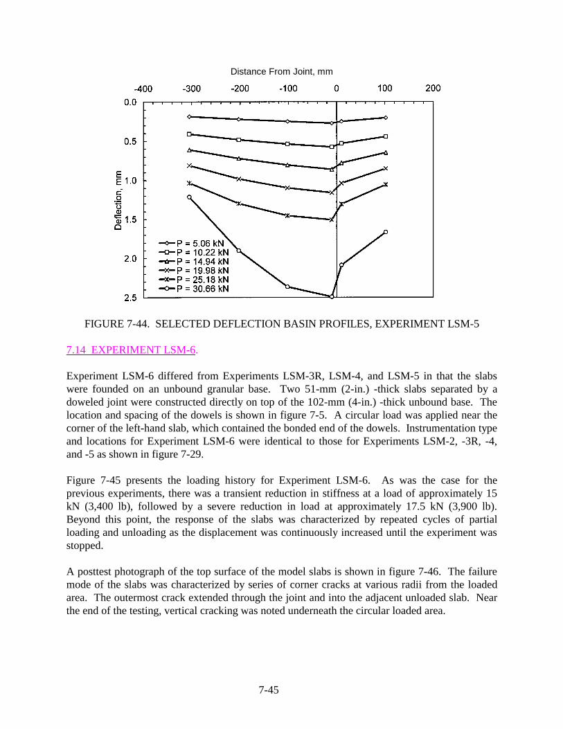
Distance From Joint, mm
FIGURE 7-44. SELECTED DEFLECTION BASIN PROFILES, EXPERIMENT LSM-5
7.14 EXPERIMENT LSM-6.
Experiment LSM-6 differed from Experiments LSM-3R, LSM-4, and LSM-5 in that the slabs were founded on an unbound granular base. Two 51-mm (2-in.) -thick slabs separated by a doweled joint were constructed directly on top of the 102-mm (4-in.) -thick unbound base. The location and spacing of the dowels is shown in figure 7-5. A circular load was applied near the corner of the left-hand slab, which contained the bonded end of the dowels. Instrumentation type and locations for Experiment LSM-6 were identical to those for Experiments LSM-2, -3R, -4, and -5 as shown in figure 7-29.
Figure 7-45 presents the loading history for Experiment LSM-6. As was the case for the previous experiments, there was a transient reduction in stiffness at a load of approximately 15 kN (3,400 lb), followed by a severe reduction in load at approximately 17.5 kN (3,900 lb). Beyond this point, the response of the slabs was characterized by repeated cycles of partial loading and unloading as the displacement was continuously increased until the experiment was stopped.
A posttest photograph of the top surface of the model slabs is shown in figure 7-46. The failure mode of the slabs was characterized by series of corner cracks at various radii from the loaded area. The outermost crack extended through the joint and into the adjacent unloaded slab. Near the end of the testing, vertical cracking was noted underneath the circular loaded area.
7-45

FIGURE 7-45. LOADING HISTORY, EXPERIMENT LSM-6
FIGURE 7-46. POSTTEST PHOTOGRAPH OF TOP SURFACE OF SLABS,EXPERIMENT LSM-6
7-46

Figure 7-47 contains selected photographs from the camera mounted just outside the transparent window in the reaction box. These photographs show the relative large displacement of the loaded slab to the left of the joint. However, no evidence of shearing can be seen in the banded layers of the unbound granular base.
FIGURE 7-47. SELECTED PHOTOGRAPHS OF JOINT REGION DURING TESTING, EXPERIMENT LSM-6
The load-displacement and strain traces from the experiment are presented in appendix B. Gage D2 failed to produce data during the experiment due to a short in the instrumentation cable. Gage D6 also failed during the conduct of the experiment. Gages D3, D4, and D5 experienced overranging during the experiment. Selected deflection basin profiles from the experiment are plotted in figure 7-48.
7-47

Distance From Joint, mm
FIGURE 7-48. SELECTED DEFLECTION BASIN PROFILES, EXPERIMENT LSM-6
7.15 COMPARISON OF EXPERIMENTAL RESULTS.
In figures 7-49 and 7-50, the load-deformation traces from D4 and D5, respectively, from Experiments LSM-2, -3R, -4, -5, and -6 have been plotted on the same graphs. These plots indicate the relative stiffness and strength of the various experimental model configurations. To compare the slopes of the five curves, instantaneous slope values were calculated for loads between 5 and 10 kN for the cases of the loaded and unloaded sides of the joint. ANOVA techniques were subsequently used to determine if a statistically significant difference in the precracking slopes could be observed. The instantaneous slope measurements failed a normality test; therefore the ANOVA was conducted based upon ranks. Differences in the median values among the experiments were greater than would be expected by chance; therefore, there was a statistically significant difference at the 0.05 significance level. A multiple pairwise comparison procedure was used to isolate the experiments that were significantly different. The results of this procedure indicated that the slope measured for Experiment LSM-6 was significantly different for that of Experiments LSM-2, -3R, -4, and -5.
7-48

FIGURE 7-49. LOAD-DEFLECTION CURVES FROM EXPERIMENTS, LOADED SIDE OF JOINT
FIGURE 7-50. LOAD-DEFLECTION CURVES FROM EXPERIMENTS, UNLOADED SIDE OF JOINT
The postcracking responses of the five experiments revealed some striking differences. As expected, the load carrying capacity of the models with stabilized bases exceeded that of the experiment without a stabilized base (Experiment LSM-2) and that for the unbound granular base (Experiment LSM-6). For the two experiments in which bonding between the slabs and base was
7-49
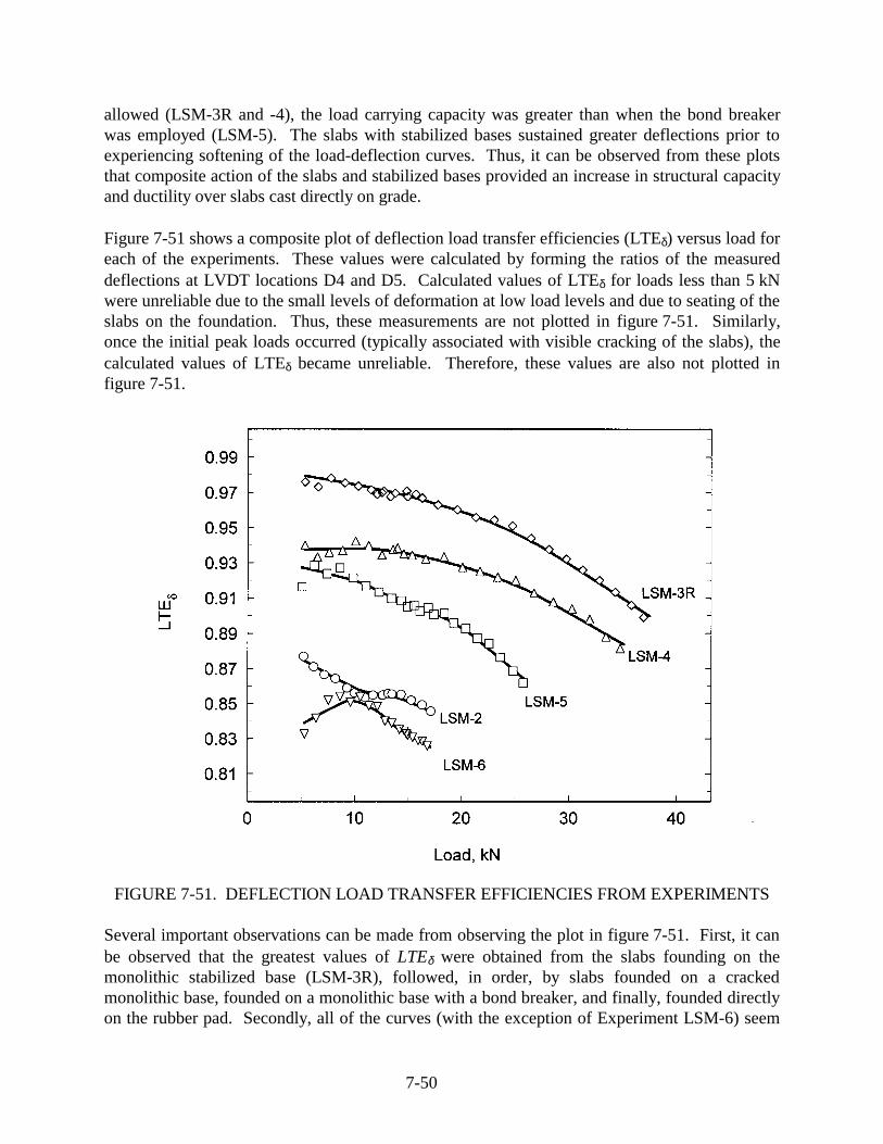
allowed (LSM-3R and -4), the load carrying capacity was greater than when the bond breaker was employed (LSM-5). The slabs with stabilized bases sustained greater deflections prior to experiencing softening of the load-deflection curves. Thus, it can be observed from these plots that composite action of the slabs and stabilized bases provided an increase in structural capacity and ductility over slabs cast directly on grade.
Figure 7-51 shows a composite plot of deflection load transfer efficiencies (LTEδ) versus load for each of the experiments. These values were calculated by forming the ratios of the measured deflections at LVDT locations D4 and D5. Calculated values of LTEδ for loads less than 5 kN were unreliable due to the small levels of deformation at low load levels and due to seating of the slabs on the foundation. Thus, these measurements are not plotted in figure 7-51. Similarly, once the initial peak loads occurred (typically associated with visible cracking of the slabs), the calculated values of LTEδ became unreliable. Therefore, these values are also not plotted in figure 7-51.
FIGURE 7-51. DEFLECTION LOAD TRANSFER EFFICIENCIES FROM EXPERIMENTS
Several important observations can be made from observing the plot in figure 7-51. First, it can be observed that the greatest values of LTEδ were obtained from the slabs founding on the monolithic stabilized base (LSM-3R), followed, in order, by slabs founded on a cracked monolithic base, founded on a monolithic base with a bond breaker, and finally, founded directly on the rubber pad. Secondly, all of the curves (with the exception of Experiment LSM-6) seem
7-50

to have the same general shape indicating the maximum load transfer efficiency occurred at low loads with decreasing effectiveness for increasing load. This phenomenon is likely caused by localized crushing of the slabs’ concrete in the region of the dowels as the loads and resulting displacements increase. This crushing occurs where high localized loads are being transferred from the concrete to the bars or visa versa. This effect has been predicted by finite element modelers (Channakeshava, Barzegar, and Voyiadjis 1993) and can also occur as the result of localized fatigue in pavement slabs under the influence of repeated service loads. The deviance from this pattern observed for Experiment LSM-6 may be caused by the nonlinear response of the unbound granular base.
Certain observations from this experimental program point to some significant challenges for modelers seeking to predict rigid pavement behavior and performance. Among these are the following challenges:
a. The presence of bonding between the slabs and base has an effect on the strength and ductility of the rigid pavement structure. The concept of the composite or “ top of the base” modulus of subgrade reaction, which involves increasing the subgrade modulus to account for stabilized bases, ignores the composite action of the slab-stabilized base structural system. This concept, which was adopted out of necessity when the only method of predicting rigid pavement behavior was the Westergaard theory, should be abandoned in favor of a more realistic model that explicitly includes the structural benefits of the stabilized base.
b. The presence and quality of stabilized base has an influence on the load transfer effectiveness of a rigid pavement joint. From the experimental data, it appears that a monolithic stabilized base provides superior joint performance. However, field observations by Grogan, Weiss, and Rollings (1996) at Dallas-Fort Worth, Stapleton (Denver), and Hartsfield (Atlanta) International Airports have indicated that the majority of both the longitudinal and transverse cracking in cement stabilized bases was found to occur under the joints in the rigid pavement surface. Thus, it may reasonably be expected that, for the majority of in-service rigid pavements, cracks are present in the stabilized base in a pattern matching the jointing pattern of the slabs. The net effect of this cracking is that the load transfer mechanism includes not only the load transfer devices (dowels, aggregate interlock, key ways) in the slab, but also some degree of load transfer due to aggregate interlock in the stabilized base. The effectiveness of this aggregate interlock in the base is likely to depend upon the magnitude and cycles of loading, quality of the stabilized base materials, and moisture and temperature (and attending volume changes) in the base.
c. The presence and degree of bonding between the slabs and the stabilized base course has an influence on the structural capacity and load transfer capability of the rigid pavement structure. Research by Wesivich, McCullough, and Burns (1987) has shown that the magnitude of friction between the slab and the base is dependent upon bearing, shear, and adhesion between the slab and the base. They also concluded that if the adhesion is great enough, the failure plane will not be at the interface between the slab and base, but rather
7-51
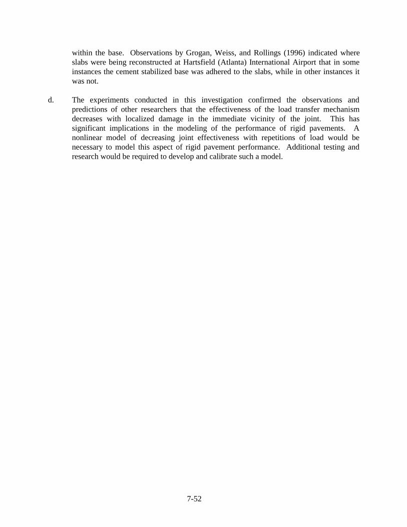
within the base. Observations by Grogan, Weiss, and Rollings (1996) indicated where slabs were being reconstructed at Hartsfield (Atlanta) International Airport that in some instances the cement stabilized base was adhered to the slabs, while in other instances it was not.
d. The experiments conducted in this investigation confirmed the observations and predictions of other researchers that the effectiveness of the load transfer mechanism decreases with localized damage in the immediate vicinity of the joint. This has significant implications in the modeling of the performance of rigid pavements. A nonlinear model of decreasing joint effectiveness with repetitions of load would be necessary to model this aspect of rigid pavement performance. Additional testing and research would be required to develop and calibrate such a model.
7-52
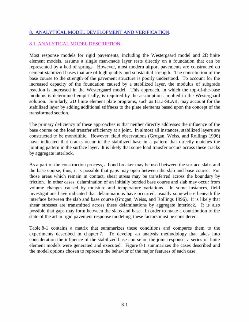
8. ANAL YTICAL MODEL DEVELOPMENT AND VERIFICATION.
8.1 ANAL YTICAL MODEL DESCRIPTION.
Most response models for rigid pavements, including the Westergaard model and 2D finite element models, assume a single man-made layer rests directly on a foundation that can be represented by a bed of springs. However, most modern airport pavements are constructed on cement-stabilized bases that are of high quality and substantial strength. The contribution of the base course to the strength of the pavement structure is poorly understood. To account for the increased capacity of the foundation caused by a stabilized layer, the modulus of subgrade reaction is increased in the Westergaard model. This approach, in which the top-of-the-base modulus is determined empirically, is required by the assumptions implied in the Westergaard solution. Similarly, 2D finite element plate programs, such as ILLI-SLAB, may account for the stabilized layer by adding additional stiffness to the plate elements based upon the concept of the transformed section.
The primary deficiency of these approaches is that neither directly addresses the influence of the base course on the load transfer effic iency at a joint. In almost all instances, stabilized layers are constructed to be monolithic. However, field observations (Grogan, Weiss, and Rollings 1996) have indicated that cracks occur in the stabilized base in a pattern that directly matches the jointing pattern in the surface layer. It is likely that some load transfer occurs across these cracks by aggregate interlock.
As a part of the construction process, a bond breaker may be used between the surface slabs and the base course; thus, it is possible that gaps may open between the slab and base course. For those areas which remain in contact, shear stress may be transferred across the boundary by friction. In other cases, delamination of an initially bonded base course and slab may occur from volume changes caused by moisture and temperature variations. In some instances, field investigations have indicated that delaminations have occurred, usually somewhere beneath the interface between the slab and base course (Grogan, Weiss, and Rollings 1996). It is likely that shear stresses are transmitted across these delaminations by aggregate interlock. It is also possible that gaps may form between the slabs and base. In order to make a contribution to the state of the art in rigid pavement response modeling, these factors must be considered.
Table 8-1 contains a matrix that summarizes these conditions and compares them to the experiments described in chapter 7. To develop an analysis methodology that takes into consideration the influence of the stabilized base course on the joint response, a series of finite element models were generated and executed. Figure 8-1 summarizes the cases described and the model options chosen to represent the behavior of the major features of each case.
8-1

TABLE 8-1. CONSIDERATIONS FOR MODEL DEVELOPMENT
Case Are Base and Slabs
Bonded? Is Base Course Cracked
Beneath Slab Joint? Experiment Most Closely
Matching Case
I No Base No Base LSM-2
II Yes No LSM-3R
III Yes Yes LSM-4
IV No No LSM-5, LSM-6
V No Yes Not in experimental matrix
C3D27R
FIGURE 8-1. ANAL YTICAL MODEL CASE DESCRIPTIONS
The slabs and base course continua were modeled by C3D27R reduced-integration, Lagrangian hexahedral elements. The joint between the slabs was modeled by JOINTC elements with stiffnesses assigned in the z direction only. Thus, the load transfer mechanism was implicitly a shear only mechanism, with no load transfer due to bending. The interface between the slabs and base course was modeled by the ABAQUS contact interaction feature. Where the base and slabs were bonded (Cases II and III) , the tied option was invoked to force the displacements of all three degrees of freedom (u, v, and w) to be equal for all node pairs across the interface. Where the
8-2

slabs and base were not bonded (Cases IV and V), the friction option was used to allow transfer of shear contact stresses across the interface. For Cases II and IV in which the base course was not cracked, ABAQUS MPCs with the tie option invoked was used to set equal displacements (u, v, and w) of corresponding node pairs across the crack. Conversely, for Cases III and V in which a crack was present in the base course, JOINTC elements were employed to allow load transfer across to the crack. Again, stiffnesses were assigned to the JOINTC elements in the z direction only, limiting load transfer to shear only. For each of the cases, the subgrade was modeled as a bed of springs using the ABAQUS foundation option. In all cases, the slabs and base were considered to be weightless.
8.2 ANAL YTICAL MODEL RESULTS.
8.2.1 Case I.
The material and structural parameters from the experimental pavement models (summarized in table 8-2) were used to develop the analytical model. Because of concerns about execution times and memory requirements, a relatively coarse mesh (figure 8-2) was adopted. The aspect ratio for the elements in the plane of the slab surface was 1:1, while the aspect ratio in the plane of the slab thickness was 4:1. The spring stiffnesses assigned to the individual JOINTC elements were calculated from the data in table 8-2 using equations 4.15 and 4.16. The loaded area was equal to that of the circular loaded area in the experimental program. The load consisted of a uniform pressure of 1 MPa, and the loaded area was 0.0104 m2 resulting in a total load of 10.4 kN.
The boundary conditions for the finite element model were selected to match those of the experiment as closely as possible. The ends of the experimental slabs were restrained by the stiff, steel reaction box and by structural steel angles embedded in the top surface of each slab and bolted to the reaction box. Thus, all three degrees of freedom were restrained (u ≡ v ≡ w ≡ 0) along these ends in the finite element model. The other sides of the experimental slabs were prevented from deforming laterally by the steel reaction box. Therefore, in the finite element model, translation perpendicular to the sides of the box was restrained (v ≡ 0). Because the sides of the box were coated with a form-release agent prior to casting the slabs, the other two degrees of freedom were not restrained.
The results from the finite element analysis were compared with results from Experiment LSM-2. In order to directly compare the load-deflection results from the finite element model to the experiment, the experimental load-deflection data were corrected to remove the nonlinearity introduced by the rubber subgrade. This was done in a manner identical to that described in chapter 7 for Experiments LSM-1A and LSM-1B. The original experimental data along with the corrected experimental data (up to a load of 10 kN) are shown in figure 8-3. The resulting experimental deflection basin profiles at a load of approximately 10 kN are shown in figure 8-4 along with the deflection basin profile from the finite element model. These data indicate that the finite element model matches the corrected experimental data well.
8-3

--
--
--
--
--
--
--
--
--
--
--
--
--
-- --
--
TABLE 8-2. APPLICABLE EXPERIMENTAL MODEL PARAMETERS
Parameter Equation No. Dimensions Value
Slabs-on-Grade Material Parameters
Es F/L2 27,600 MPa
µs — 0.18
h L 0.051 m
k F/L3 90 MPa/m
Slabs-on-Grade Structural Parameters
� 3.1 L 0.243 m
ε L 0.0508 m
ε� � — — 0.209
Joint Material Parameters
Ed F/L2 200,000 MPa
µd — 0.30
K F/L3 407,000 MPa/m
Joint Structural Parameters
s L 0.102 m
d L 0.00635 m
Id L4 7.98×10⁻¹¹ m 4
Az 4.12 L2 28.5×10⁻⁶ m 2
Gd 4.11 F/L2 76,900 MPa
ω L 0.00159 m
φ 4.10 34.7
C 4.9 F/L 112 MN/m
β 4.8 L-1 79.8 m-1
DCI 4.7 F/L 15.2 MN/m
D 4.6 F/L 15.1 MN/m
f = D/sk � 6.79
q = D/s F/L2 148 MN/m/m
8-4

E = 27,600 MPa q = 148 MN/m/m p = 1 MPa
µ= 0.18 kcorner = 0.47 MN/m A = 0.0104 m2
h = 0.051 m kedge = 0.94 MN/m P = 0.0104 MN
k = 90 MPa/m kinterior = 1.88 MN/m a = 0.0575 m
� = 0.243 m a/ � = 0.237
FIGURE 8-2. FINITE ELEMENT MODEL, CASE I
FIGURE 8-3. RAW AND CORRECTED DISPLACEMENTS, EXPERIMENT LSM-2
8-5

Deflection Basin Profile at P = 10 kN
Distance From Joint, mm
FIGURE 8-4. EXPERIMENTAL AND ANAL YTICAL DEFLECTION BASIN PROFILES, EXPERIMENT LSM-2
Figure 8-5 shows a plot of LTEδ (calculated as the ratio of LVDTs D5 and D4) as a function of applied load. Superimposed on this data is the deflection load transfer effic iency predicted at the location of LVDTs D5 and D4 by the finite element model. Again, the agreement between the model and the experimental data is acceptable over the linear range of response of the experimental slabs. At loads above approximately 17 kN, significant cracking occurred in the experiment, thus changing the experimental boundary conditions.
FIGURE 8-5. COMPARISON OF EXPERIMENTAL DEFLECTION LOAD TRANSFER EFFICIENCY WITH ANALYTICAL VALUE, EXPERIMENT LSM-2
8-6

Based upon these results it was concluded all aspects of the finite element model, including the density of finite element mesh, the modeling of the load transfer at the joints, and the boundary conditions imposed on the slab by the reaction box, were adequate.
8.2.2 Case II.
Figure 8-6 shows a diagram of the 3D finite element mesh used to predict the response from Experiments LSM-3R. In plan view, the mesh was identical to the mesh employed for Experiment LSM-2. The surface layer consisted of two slabs separated by a joint, which was modeled using the ABAQUS JOINTC elements. The individual spring stiffnesses assigned to the JOINTC elements across the joint in the slabs were identical to those employed for the finite element model of Case I (Experiment LSM-2).
Eslab = 27,600 MPa Ebase = 1,410 MPa p = 1 MPa
µslab = 0.18 µbase = 0.20 A = 0.0104 m2
hslab = 0.051 m hbase = 0.038 m P = 0.0104 MN
k = 90 MPa/m a = 0.0575 m
qslab = 148 MN/m/m
FIGURE 8-6. FINITE ELEMENT MODEL, CASES II, III, IV, AND V
The material and structural properties of the slabs and subgrade were identical to those described in table 8-2. Additional material and structural parameters for the base course are listed in table 8-3.
8-7

--
-- --
--
--
�
TABLE 8-3. APPLICABLE EXPERIMENTAL MODEL PARAMETERS FOR BASE
Parameter Equation No. Dimensions Value
Base Material Parameters
Eb F/L2 1,410 MPa
µb 0.20
h L 0.038 m
Base Structural Parameters
� b 8.1 L 13.056 m
B 8.2 2.903
Two additional structural parameters, used by Kuo (1994), were introduced to describe the structural properties of the base course. The radius of relative stiffness defined as follows:
� b= Eb (8.1)k (1- µb )
The base factor relates the structural properties of the base and slab as follows:
B= � hb b (8.2)
The finite element model was extended in the vertical direction (z direction) to include the base course. The base course was modeled by a single layer of ABAQUS C3D27R hexahedral elements with aspect ratios of 1:1 in the plane of the base surface and 2.67:1 in the plane of the base thickness. The nodes along the interface between the slab and base were tied so that no delaminations or slip occurred between the slabs and base course. The lower surfaces of the elements in the base course were supported by a bed of springs using the ABAQUS foundation option.
As was the situation for the Case I finite element model, the boundary conditions were chosen to match as closely as possible the experimental conditions. The boundary conditions, as indicated in figure 8-6, were thus the same as those used for Case I.
The results from the finite element model were compared with data from Experiment LSM-3R. Figure 8-7 shows a plot of LTEδ versus load from Experiment LSM-3R along with the value of LTEδ predicted from the Case II finite element model at the location of the LVDT array in the experiment. The finite element model predicted almost perfect joint effic iency (LTEδ = 0.998). Figure 8-8 shows the deflection basin profile (raw data, no corrections applied) from Experiment LSM-3R at a load of approximately 10 kN plotted alongside the analytical deflection basin profile for that load. The magnitude of the deflections predicted less than that observed in the experiment.
8-8

FIGURE 8-7. COMPARISON OF EXPERIMENTAL DEFLECTION LOAD TRANSFER EFFICIENCY WITH ANALYTICAL VALUE, EXPERIMENT LSM-3R
Distance From Joint, mm
FIGURE 8-8. EXPERIMENTAL AND ANAL YTICAL DEFLECTION BASIN PROFILES, EXPERIMENT LSM-3R
A second finite element run was made with the Case II model. In this run, the stiffness of the joint was decreased by a factor of 100 from q = 148 MN/m/m to q = 1.48 MN/m/m. As indicated in figure 8-9, decreasing the stiffness of the joint by two orders of magnitude had little effect on the resulting LTEδ. In Case II, the slabs and base were not free to separate. Furthermore, the base was monolithic, and thus the slabs are forced to have equal displacements at the intersection of the joint with the slab/base course interface. Because of this effect, there was essentially no
8-9

differential movement across the joint. Thus, the magnitude of the stiffness of the JOINTC elements makes virtually no difference because the differential displacements across the joint are small.
FIGURE 8-9. VARIATION OF ANALYTICAL DEFLECTION LOAD TRANSFER EFFICIENCY WITH JOINT STIFFNESS, CASE II
8.2.3 Case III .
The finite element model employed for Case III was identical to that employed for Case II with one major exception: a crack with aggregate interlock was present in the base course model. Material and structural properties for the model were identical to those listed in tables 8-1 and 8-3. The stiffness of the joint, qjoint , for Case III was identical to that for Cases I and II. The effect of aggregate interlock in the base course on joint response was investigated. Aggregate interlock across the crack was modeled using ABAQUS JOINTC elements connecting corresponding node pairs across the crack. A range of conditions were modeled, varying from the case of an open crack in the base with no load transfer to the case of a monolithic base, by choosing a spectrum of values of the crack stiffness parameter qbase. The individual spring constants (κ) for the joint and base were calculated from the�qbase and qjoint using equations 4.15 and 4.16.
The results from these analyses are plotted in figure 8-10. The horizontal axis is the ratio of qbase
to qjoint, while the vertical axis is LTEδ calculated at the location of the LVDT array in the experimental program. For the case of a doweled joint with no aggregate interlock, qjoint is a function of the dowel diameter, dowel spacing, and joint opening. However, qbase is an unknown quantity which may approach zero in the case of an open crack (no aggregate interlock) to near infinity in the case of a monolithic base course.
8-10

Several important observations can be made concerning the analytical curve in figure 8-10. Results from the finite element analyses indicate that the amount of load transfer in the base influences the deflection load transfer at the joint. As would be intuitively expected, the deflection load transfer efficiency increases with increasing shear stiffness across the crack in the base course.
The deflection load transfer efficiencies from Experiments LSM-3R and LSM-4 are also shown in figure 8-10. The data from LSM-4 indicates that one would predict that the crack stiffness due to aggregate interlock in the base course was over twice the stiffness of the doweled joint. However, this observation is irrational because the dowels in the slabs should provide more shear stiffness than the aggregate interlock in the base. Similarly, the data from LSM-3R indicates that the experimental deflection load transfer efficiency intersects the curve in a location somewhat below the point predicted for a monolithic base.
FIGURE 8-10. VARIATION OF ANALYTICAL DEFLECTION LOAD TRANSFER EFFICIENCY WITH CHANGES IN AGGREGATE INTERLOCK IN CRACKED BASE, CASE III
The stiffness of the doweled joint can be decomposed into components from shearing action in the dowel, bending action in the dowel, and from direct bearing (or aggregate interlock) across the joint as follows:
q joint = qdowel shear+ qdowel bending+ qaggregateinterlock (8.3)
8-11

Most researchers have concluded that the component due to dowel bending is negligible, particularly for the ranges of joint openings which typically occur in airport pavements. Therefore, the joint stiffness can be thought of as the sum of the components from dowel shear and from aggregate interlock. In the case of the experimental program, the dowel shear component may be calculated directly from the dowel diameter, dowel spacing, and joint opening. Even though the joint opening in the experiments contained a Teflon strip to minimize load transfer due to direct bearing, it is likely that direct bearing made some contribution to the stiffness of the joint. If direct bearing contributed to the stiffness of the joint, qjoint is greater than that calculated from the dowels alone. As qjoint increases, the ratio of qbase to qjoint decreases. Thus, the curve in figure 8-10 would be translated to the left, as indicated in figure 8-11. This postulated shift in the locus of the curve would result in a rational intersection of the experimental data with the analytical curve.
FIGURE 8-11. POSTULATED SHIFT IN ANALYTICAL CURVE DUE TO DIRECT BEARING IN JOINT, CASE III
Deflection basins from selected Case III r uns along the location of the experimental LVDT array are plotted versus the experimental deflection basin profile from Experiment LSM-4 at a load of approximately 10 kN in figure 8-12. The deflection on the loaded (left) side of the joint for the case where qbase/q joint = 0.1 is very nearly the same as the experimental deflection at that location. However, the deflection just across the joint is less than that observed in the experiment. Also note that as the q ratio increases, the ratio of deflections across the joint becomes closer to unity.
8-12

FIGURE 8-12. EXPERIMENTAL AND ANAL YTICAL DEFLECTION BASIN PROFILES, EXPERIMENT LSM-4
8.2.4 Case IV.
In Case IV, the base was considered to be monolithic. However, the contact interaction feature was implemented between the base course and the slabs allowing slip to occur between the slabs and base as well as gaps to open. Coulomb friction was modeled on the contact surfaces with a range of coefficients of static friction from 0.1 to 100. A coefficient of friction greater than 1 represents a shear stress which is greater than the normal pressure causing the shear stress. This condition, which may not be realistic, is nonetheless instructive to consider as a modeling tool.
Figure 8-13 shows a plot of deflections and LTEδ versus coefficient of static friction. The upper plot in figure 8-13 shows that the magnitude of deflection on both the loaded and unloaded sides of the joint decreases with an increase in friction. However, the deflection on the loaded side decreases more sharply than the deflection on the unloaded side as friction increases. This gives rise to the trend of decreasing LTEδ as the coefficient of friction increases, as shown in the lower plot of figure 8-13. A less than 1 percent difference in LTEδ was predicted as the coefficient of friction rose from 0.1 to 100. These values of LTEδ were at least 8 percent less than those for Case II (fully bonded slabs and base, no crack in base).
8-13

FIGURE 8-13. VARIATION OF ANALYTICAL DEFLECTION LOAD TRANSFER EFFICIENCY WITH FRICTION BETWEEN BASE COURSE AND SLAB, CASE IV
Figure 8-14 shows a plot of the vertical deflection profiles calculated along the edge of the model at the top of the base course and the bottom of the slabs for the coefficient of friction = 1. These curves clearly indicate that gaps were forming between the slabs and base course on both the loaded and unloaded side of the joint. The largest gap was located on the unloaded side of the joint. This response was typical of that predicted across the range of coefficient of friction studied. Figure 8-15 shows a plot of the gap between the slabs and base course, denoted as Δz, as a function of distance from the joint and friction. Clearly, gaps were present in all cases; the largest gaps occurred for the lowest value of coefficient of friction.
8-14

Coefficient of Friction = 1 Distance From Joint, mm
FIGURE 8-14. VERTICAL DEFLECTION PROFILES ALONG EDGE ILLUSTRATING GAP BETWEEN SLAB AND BASE, CASE IV
Distance From Joint, mm
FIGURE 8-15. GAP OPENING BETWEEN SLAB AND BASE, CASE IV
Figure 8-16 shows profiles of the horizontal deformations for selected nodes on the top of the base course and on the bottom of the slab. A positive deformation indicates movement to the right, while negative values indicate movement to the left. This plot indicates that the slabs were moving relative to one another. The top of the base was moving right on the loaded side of the joint and left on the unloaded side. Conversely, the loaded side moved left while the unloaded slab moved right. The discontinuity between the slabs at the joint shows clearly in this plot. Figure 8-17 shows a plot of differential horizontal movement between the slabs and base as a
8-15

function of distance from the joint and friction. As expected, the largest differential movements occurred for the lowest value of coefficient of friction.
Coefficient of Friction = 1
Distance From Joint, mm
FIGURE 8-16. HORIZONTAL DEFLECTION PROFILES ALONG EDGE ILLUSTRATING SLIP BETWEEN SLAB AND BASE, CASE IV
Distance From Joint, mm
FIGURE 8-17. RELATIVE SLIP BETWEEN SLAB AND BASE, CASE IV
8-16

Figure 8-18 shows plots of the deflection basin profiles from Cases II and IV compared with the deflection basin profiles from Experiment LSM-5. It is obvious that the deflection basin from the run with the lowest coeffic ient of friction most closely matches that of the experiment.
Distance From Joint, mm
FIGURE 8-18. EXPERIMENTAL AND ANAL YTICAL DEFLECTION BASIN PROFILES, EXPERIMENT LSM-5
8.2.5 Case V.
Case V was distinguished from the other four cases in that the base course was considered to be cracked with some value of aggregate interlock across the crack, and the base course and slabs were not bonded allowing gaps to form between the slabs and base. Where the slabs and base were in contact, shear stress was transmitted via friction between the slabs and base course.
The joint response over a range of coefficients of friction and aggregate interlock across the crack in the base are plotted in figure 8-19. As expected, these results indicate that joint efficiency decreases as aggregate interlock across the crack in the base decreases. It also indicates that the joint efficiency decreases with increasing values of the coefficient of friction, as was found for Case IV. In figure 8-20, results from the Case III analyses have been plotted along with the results from Case V. It can be seen from figure 8-20 that allowing gaps to form between the slab and base course tends to flatten the joint response curves and thereby reduces the range of possible joint efficiencies compared to a cracked base.
8-17

FIGURE 8-19. VARIATION OF ANALYTICAL DEFLECTION LOAD TRANSFEREFFICIENCY WITH FRICTION BETWEEN BASE COURSE ANDSLAB AND AGGREGATE INTERLOCK ACROSS CRACK, CASE V
FIGURE 8-20. COMPARISON OF JOINT RESPONSES FROM CASES III AND V
8-18

8.3 SLAB/BASE INTERACTION AND JOINT RESPONSE.
The analytical results reported in this chapter indicate that a wide range of joint efficiencies are possible from a given joint subjected to a given loading depending on the following factors:
a. Presence of stabilized base layer.
b. The amount of load transfers by aggregate interlocks across cracks in the stabilized base layer directly below slab joints.
c. The bonding properties between concrete slabs and stabilized base layer as well as interface conditions between these two layers.
These effects are illustrated by the bar chart shown in figure 8-21. This plot compares the calculated joint efficiencies from Cases III, IV, and V. It can be seen from this graph that the case of the monolithic base bonded to the slabs gives nearly perfect joint efficiency. If the monolithic base is cracked, the joint effic iency is decreased, with a trend of decreasing joint efficiency as the aggregate interlock across the crack decreases. If gaps are allowed to form between the base and slabs, joint efficiency is decreased compared to the bonded cases, and the coefficient of friction between the slabs and base has only a small effect on the load transfer obtained.
FIGURE 8-21. COMPARISON OF JOINT RESPONSES FROM CASES III, IV, AND V
8-19

Figure 8-22 shows a plot of the maximum load transfer values obtained in the experimental program (chapter 7) compared with the ranges of values calculated from the analyses described in this chapter. For the analytical data, the solid bar represents the lower bound of possible values of LTEδ, while the error bar represents the upper bound values. In all cases, with the exception of Case IV, the experimental response is within the range of possible responses predicted by the experiments. This experimental and analytical agreement lend credibility to the validity of the analytical models.
FIGURE 8-22. COMPARISON OF JOINT RESPONSES FROM FINITE ELEMENT MODELS AND EXPERIMENTS
The implications of these responses upon the response and performance of rigid pavements in the field is not explicitly predicted by the analytical model. However, it is possible to discuss in general terms the potential impact. Refer to figure 8-23. Suppose a particular joint were constructed on a stabilized base such that the base course was initially monolithic and the base and slabs were initially bonded. Over a period of time, here indicated by aircraft departures, repeated cycles of aircraft and/or environmental loading may result in cracking of the base directly beneath the joint. Depending upon the degree of aggregate interlock across the crack in the base, the finite element analyses indicated that a range of responses (indicated by the two solid curves in figure 8-23) is possible.
Next, suppose that an identical joint were constructed in the same manner. However, in this case, suppose that the base and slabs were debonded by repeated cycles or aircraft or environmental loading such that it was possible that gaps could form between the slabs and base in the vicinity of the joint. For the sake of argument, suppose that the base were monolithic. The
8-20

finite element analyses indicate a range of possible responses, depending upon the amount of shear stresses transmitted across the interface by friction, denoted by the dashed curves in figure 8-23. Note that the range of possible responses is much less than that possible due to cracking of the base.
FIGURE 8-23. POSSIBLE IMPLICATIONS OF SLAB/BASE INTERACTION ON JOINT PERFORMANCE
Finally, suppose that the identical joint were again constructed in the same manner. Now, in this case, suppose that aircraft or environmental loadings cause the base to crack beneath the joint and also cause delamination or debonding between the slabs and base. Again the finite element models indicated a range of possible responses plotted as dash-dot curves in figure 8-23. Again, the range of potential responses is much less than that for the cracked base alone. However, as expected, the efficiency of a joint associated with a cracked and debonded base is predicted to be less than that of the joint associated with a debonded base without a crack.
It should be noted that the exact values of LTEδ obtained in a particular case depend not only on the slab/base interaction factors but also upon the slab and base geometry, subgrade strength, material properties, and load geometry. Therefore, the values plotted on the vertical axis in figure 8-23 are intended to be representative values of the LTEδ obtained in these analytical cases.
8-21/8-22

9. CONCLUSIONS AND RECOMMENDATIONS.
9.1 CONCLUSIONS.
The response of the rigid pavement slab-joint-base structural system is complex, and accurately predicting the response of such a system requires a significant degree of analytical sophistication. The research reported in this report has defined some essential features required to adequately model the system and has demonstrated a technique to develop a comprehensive 3D finite element model of the rigid pavement slab-joint-foundation structural system. These findings represent a significant advancement in the state of the art of rigid pavement response modeling. Specifically, the following conclusions can be drawn from this study:
a. Analysis of experimental data obtained by the Corps of Engineers in the 1950's confirms the usefulness of the concepts of dimensionless joint stiffness as a means of characterizing the response of the doweled joint. Thus, the response of both the aggregate interlock joint and the doweled joint can be characterized by the same family of curves. Explicit modeling of the dowel in the 3D finite element model, while perhaps useful for research purposes, is unnecessary for predicting the gross response of the structural system. The usefulness of the dimensionless joint stiffness for characterizing the response of the keyed joint was not addressed by this research. The ease of application of the concepts of dimensionless joint stiffness has been increased by the development of closed-form equations based upon the theoretical developments of Skarlatos (1949).
b. For most practical rigid pavement slabs, the classical Kirchoff assumptions, adopted by Westergaard and Skarlatos, lead to small errors in predicting edge stresses. Results from 3D finite element models show that the maximum edge stress does not occur at the edge of the slab but at some finite distance from the edge. Fortunately, the Westergaard edge stress is conservative; for most rigid pavement slabs, the maximum edge stress will occur within 0.1 � of the edge of the slab and will be approximately 10 percent less than that predicted by the Westergaard theory.
c. Experimental evidence from this research suggests that the joint efficiency depends upon the presence and condition of a stabilized base. The presence of cracking in the base and the degree of bonding between the slabs and stabilized base course influences the structural capacity and load transfer capability of the rigid pavement structure. The greatest experimental values of joint efficiency were obtained from the slabs founding on the monolithic stabilized base followed, in order, by slabs founded on a cracked monolithic base, founded on a monolithic base with a bond breaker, and finally, founded directly on the rubber pad. Maximum load transfer efficiency occurs at low loads with decreasing effectiveness for increasing load. This phenomenon is likely caused by localized crushing of the slabs’ concrete in the region of the dowels as the loads and resulting displacements increase.
d. The finite element models developed in this research indicate that a comprehensive 3D finite element modeling technique provides a rational approach to modeling the structural
9-1

response of the jointed rigid airport pavement system. Modeling features which are required include explicit 3D modeling of the slab continua, load transfer capability at the joint (modeled springs between the slabs), explicit 3D modeling of the base course continua, aggregate interlock capability across the cracks in the base course (again, modeled by springs across the crack), and contact interaction between the slabs and base course. The contact interaction model feature must allow gaps to open between the slab and base. Furthermore, where the slabs and base are in contact, transfer of shear stresses across the interface via friction should be modeled.
9.2 RECOMMENDATIONS.
The following recommendations are drawn from this research:
a. Mechanistic design criteria for doweled joints should be developed using the concepts of dimensionless joint stiffness in concert with the closed-form Westergaard-type solution for load transfer in rigid pavements. Given the slab thickness, support conditions, and loading, it is possible to use these developments to establish criteria for dowel diameter and spacing for a critical joint opening. These criteria should then be verified by full-scale testing.
b. The concept of the composite or top-of-the-base modulus of subgrade reaction ignores the composite action of the slab-stabilized base structural system. This concept should be abandoned in favor of a more realistic model that explicitly includes the structural benefits of the stabilized base.
c. Certain issues pertaining to the effects on new- and future-generation aircraft and rigid pavement behavior and performance can be addressed by the finite element modeling techniques developed in this research. A research study should be initiated to study the effects of multiple-wheel loadings on the response of jointed rigid pavements.
d. The effects of environmental factors on the findings of this research should be investigated. It should be possible to add to the analytical complexity of this research by superimposing the effects of temperature and moisture gradients on the response of the rigid pavement structure. With the tools presented in this study, it is possible to develop and implement an algorithm which could change the joint effic iency with joint opening.
e. The 3D finite element modeling technique presented in this dissertation is suited to studying more complex material behavior which may affect pavement performance. For example, fracture mechanics concepts could be used to study the effects of repeated traffic loadings on rigid pavement structures in view of a possible replacement for the current Minor’s hypothesis fatigue laws.
f. The results of this study point to some critical issues which should be considered in developing test plans for its full-scale, instrumented test facility currently under construction. Specifically, instrumentation should be installed to detect the presence of
9-2

cracking in the stabilized base course, particularly directly beneath the joint. Also, instrumentation should be selected and installed to detect the presence of gaps between the slabs and base course.
g. The incremental finite element analysis procedure used to solve the contact interaction problem can be computer intensive. In the event that solution times and memory requirements are greater than the available computer resources, the slabs can be modeled by thick plate or shell elements with little sacrifice in accuracy. However, the capability to predict load transfer across cracks in the base course and debonding between the slabs and base are critical and must be retained.
9-3/9-4

10. REFERENCES.
Bathe, K. J., 1982. Finite Element Procedures in Engineering Analysis, Englewood Cliffs, NJ: Prentice-Hall, Inc.
Channakeshava, C., F. Barzegar, and G. Z. Voyiadjis, 1993. “Nonlinear FE Analysis of Plain Concrete Pavements with Dowel Joints,” Journal of Transportation Engineering, Vol. 119, No. 5, pp. 763-781.
Corps of Engineers, 1954. “A Model Study of the Effect of High Contact Pressures on Stresses in Rigid Pavements,” Mariemont, OH: Ohio River Division Laboratories.
Desai, C. S. and J. F. Able, 1972. Introduction to the Finite Element Method, New York: Van Nostrand Reinhold Company.
Department of the Army, 1987. Materials Testing, FM 5-530, Washington: Headquarters, Department of the Army.
Fagan, M. J., 1992. Finite Element Analysis, Essex, UK: Longman Scientific and Technical.
Federal Aviation Administration, 1995. “Airport Pavement Design for the Boeing 777 Airplane,” Advisory Circular AC 150/5320-16, Washington: Department of Transportation, Federal Aviation Administration.
Friberg, B. F., 1940. “Design of Dowels in Transverse Joints of Concrete Pavements,” Transactions of the American Society of Civil Engineers, Vol. 105, pp. 1076-1095.
Grogan, W. P., C. A. Weiss, Jr., and R. S. Rollings, 1996. “Stabilized Base Courses for Advanced Pavement Design, Report 1: Literature Review and Field Performance Data,” FAA Technical Center, Atlantic City International Airport, NJ, DOT/FAA/AR-97/65.
Hammons, M. I. and A. M. Ioannides, 1995. “Advanced Pavement Design: Finite Element Modeling for Rigid Pavement Joints, Report I: Background Investigation,” DOT/ FAA/AR-95/85, Federal Aviation Administration, Atlantic City International Airport, NJ.
Ioannides, A. M., 1984. “Analysis of Slabs-On-Grade for a Variety of Loading and Support Conditions,” Ph.D. thesis, Urbana, IL: University of Illinois.
Ioannides, A. M. and G. T. Korovesis, 1990. “Aggregate Interlock: A Pure-Shear Load Transfer Mechanism,” Transportation Research Record 1286, Washington: Transportation Research Board, pp. 14-24.
Ioannides, A. M. and G. T. Korovesis, 1992. “Analysis and Design of Doweled Slab-on-Grade Pavement Systems,” Journal of Transportation Engineering, Vol 118, No. 6, pp. 745-768.
Ioannides, A. M. and M. I. Hammons, 1996. "A Westergaard - Type Solution for the Load Transfer Problem,” presented at 1996 Annual Meeting, Transportation Research Board, Washington, DC.
10-1

Korovesis, G. T., 1990. “Analysis of Slab-On-Grade Pavement Systems Subjected to Wheel and Temperature Loadings,” Ph.D. thesis, Urbana, IL: University of Illinois.
Kuo, C. M., 1994. “Three-Dimensional Finite Element Analysis of Concrete Pavement,” Ph.D. dissertation, Urbana, IL: University of Illinois.
Pickett, G. and G. K. Ray, 1951. “I nfluence Charts for Concrete Pavements,” Transactions of the American Society of Civil Engineers, Vol. 116, pp. 49-73.
Rollings, R. S. and D. W. Pittman, 1992. “Field Instrumentation and Performance Monitoring of Rigid Pavements,” Journal of Transportation Engineering, Vol 118, No. 3, pp. 361-370.
Schnobrich, W. C., 1990. “Structural Analysis, Part 2. Continua: The Finite Element Method,” In Structural Engineering Handbook, Third Edition, E. H. Gaylord, Jr. and C. N. Gaylord (eds.), New York: McGraw-Hill.
Skarlatos, M. S., 1949. “Deflections and Stresses in Concrete Pavements of Airfields With Continuous Elastic Joints,” Mariemont, OH: Ohio River Division Labs.
Tabatabaie-Raissi, A. M., 1978. “Structural Analysis of Concrete Pavement Joints,” Ph.D. dissertation, Urbana, IL: University of Illinois.
Timoshenko, S. and S. Woinowsky-Krieger, 1959. Theory of Plates and Shells, New York: McGraw-Hill Book Company.
Wesevich, J. W., McCullough, B. F., and Burns, N. H., 1987. “Stabilized Subbase Friction Study for Concrete Pavements,” Research Report 459-1, Austin, Texas: Center for Transportation Research, University of Texas at Austin.
Westergaard, H. M, 1923. “Om Beregning Af Plader Paa Elastisk Underlag Med Særligt Henblik Pass Ppørgsmaalet Om Spændinger I Betonveje,” Ingeniøren, No. 42, pp. 513-524. (In Danish).
Westergaard, H. M., 1926. “Stresses in Concrete Pavements Computed by Theoretical Analysis,” Public Roads, Vol. 7, No. 2, pp. 25-35.
Westergaard, H. M., 1928. “Spacing of Dowels,” Proceedings, Highway Research Board, No. 8., Washington: Highway Research Board, pp. 154-158.
Westergaard, H. M., 1933. “Analytical Tools for Judging Results of Structural Tests of Concrete Pavements,” Public Roads, Vol. 14, No. 10, pp. 129-151.
Westergaard, H. M., 1939. “Stresses in Concrete Runways of Airports,” Proceedings, Highway Research Board, No. 19, Washington: National Research Council, pp. 197-205.
Westergaard, H. M., 1948. “New Formulas for Stresses in Concrete Pavements of Airfields,” Transactions, American Society of Civil Engineers, Vol. 113, pp. 425-444.
10-2

APPENDIX AALGORITHM FOR ASSIGNING SPRING STIFFNESSES TO
NODES USING THE ABAQUS “JOINTC” OPTION
PROBLEM STATEMENT
It is desired to represent the stiffness of a rigid pavement joint in ABAQUS using a 3D finite element model of the rigid pavement slabs. Each node on the joint face of a slab will be connected to the corresponding node on the joint face of the adjacent slab with a spring element. The algorithm described in this appendix provides a rational way to distribute the joint stiffness per unit length along the joint to the nodes along the joint. The ABAQUS element chosen for this study is the “JOINTC” element, a general, nonlinear spring and dashpot element which can have stiffness (and damping, as well) in three orthogonal directions. For most purposes of this study, the elements will be assigned stiffness values assigned in the vertical direction only. Furthermore, a linear force-displacement relationship will be assumed. Because all analyses are static, damping will be of no consequence.
ASSUMPTIONS
1. Let nodes be equally spaced in the y direction. Let the distance between nodes be given by 2a (figure A-1).
2. Let nodes by equally spaced in the z direction. Let the distance between nodes by given by 2b.
3. Let the number of rows of nodes be given by NR and the number of columns of nodes by given by NC.
4. Let the length of the joint to be modeled be given by λ.
5. Let the joint stiffness per unit length be given by q (Units: F/L2).
6. Let κ be the unit spring stiffness (Units: F/L).
GEOMETRY
1. There are three types of nodes: corner, edge, and interior (see figure A-1).
2. The contributing areas for each type of node are the following:
a. Corner node: AC = ab
b. Edge node: AE = 2ab
c. Interior node: AI = 4ab
A-1

FIGURE A-1. FACE OF TYPICAL ONE-LAYER 3D FINITE ELEMENT MESH SHOWING LOCATION OF NODES
3. Develop general statements for the number of each type of node as a function of NC andNR.
a. Number of corner nodes = 4
b. Number of edge nodes = 2(NR + NC -4)
c. Number of interior nodes = (NR - 2)(NC - 2)
SOLVE FOR SPRING STIFFNESSES AS A FUNCTION OF q:
1. Assign spring stiffness to types of node based on contributing areas:
a. Corner node: κ
b. Edge node: 2κ
c. Interior node: 4κ
A-2

2. Set joint stiffness equal to sum of spring stiffnesses.
q x λ = κ x (number of corner nodes) + 2κ (number of edge nodes) + 4κ x (number of interior nodes)
= κ (4) + 2κ[2(NR + NC - 4)] + 4κ(NR - 2)(NC -2)
= 4κ(1 + NR + NC - 4 + NRNC - 2NR - 2NC +4)
= 4κ(NR - 1)(NC - 1)
Therefore:
qλκ =
4(NR − 1)(N C − 1)
A-3/A-4

APPENDIX BCOMPILATION OF INSTRUMENTATION TRACES FROM EXPERIMENTS
FIGURE B-1. GAGES D1 THROUGH D4, EXPERIMENT LSM-1A
B-1

FIGURE B-2. GAGES D5 THROUGH D7, EXPERIMENT LSM-1A
B-2

FIGURE B-3. GAGES D8 AND D9, EXPERIMENT LSM-1A
B-3

FIGURE B-4. GAGES S1 THROUGH S4, EXPERIMENT LSM-1A
B-4
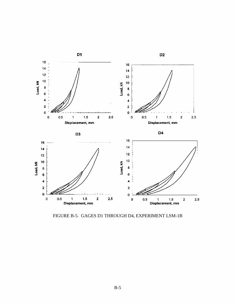
FIGURE B-5. GAGES D1 THROUGH D4, EXPERIMENT LSM-1B
B-5

FIGURE B-6. GAGES D5 AND D6, EXPERIMENT LSM-1B
B-6

FIGURE B-7. GAGES S1 THROUGH S4, EXPERIMENT LSM-1B
B-7

B-8

FIGURE B-9. GAGES D7 THROUGH D10, EXPERIMENT LSM-2
B-9

B-10

FIGURE B-11. GAGE S7, EXPERIMENT LSM-2
B-11
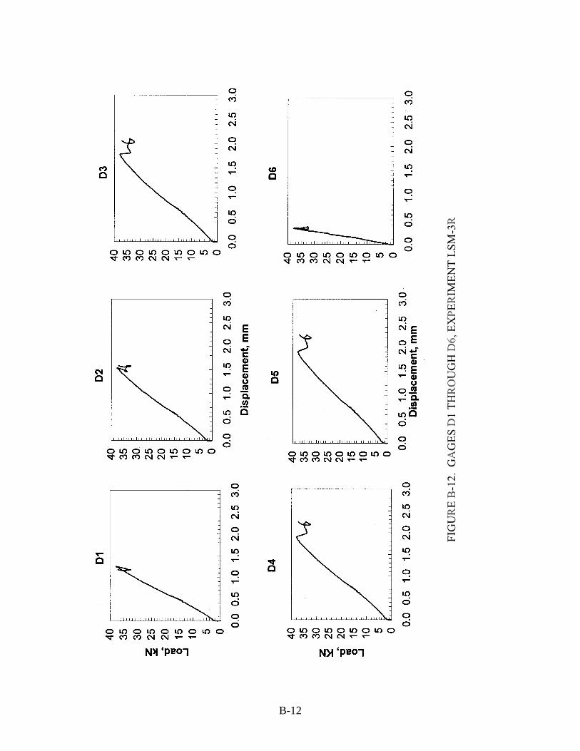
B-12

FIGURE B-13. GAGES D7 THROUGH D10, EXPERIMENT LSM-3R
B-13

B-14

FIGURE B-15. GAGE S7, EXPERIMENT LSM-3R
B-15

B-16
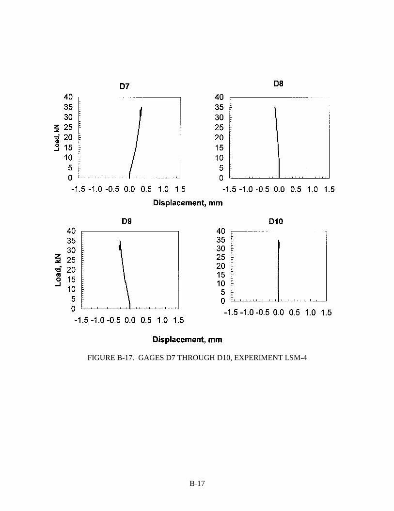
FIGURE B-17. GAGES D7 THROUGH D10, EXPERIMENT LSM-4
B-17

B-18

FIGURE B-19. GAGE S7, EXPERIMENT LSM-4
B-19

B-20

FIGURE B-21. GAGES D7 THROUGH D10, EXPERIMENT LSM-5
B-21

B-22

FIGURE B-23. GAGE S7, EXPERIMENT LSM-5
B-23

B-24

FIGURE B-25. GAGES D7 THROUGH D10, EXPERIMENT LSM-6
B-25

B-26

FIGURE B-27. GAGE S7, EXPERIMENT LSM-6
B-27/B-28