DOT/FAA/AR-05/27 Real-Time Scheduling Analysis · Real-Time Scheduling Analysis ... The first job was to explore and report the industry approaches to scheduling real-time ... and

DOT/FAA/AR-05/27 Office of Aviation Research and Development Washington, D.C. 20591

Real-Time Scheduling Analysis November 2005 Final Report This document is available to the U.S. public through the National Technical Information Service (NTIS), Springfield, Virginia 22161.

U.S. Department of Transportation Federal Aviation Administration

NOTICE

This document is disseminated under the sponsorship of the U.S. Department of Transportation in the interest of information exchange. The United States Government assumes no liability for the contents or use thereof. The United States Government does not endorse products or manufacturers. Trade or manufacturer's names appear herein solely because they are considered essential to the objective of this report. This document does not constitute FAA certification policy. Consult your local FAA aircraft certification office as to its use. This report is available at the Federal Aviation Administration William J. Hughes Technical Center's Full-Text Technical Reports page: actlibrary.tc.faa.gov in Adobe Acrobat portable document format (PDF).

Technical Report Documentation Page 1. Report No. DOT/FAA/AR-05/27

2. Government Accession No. 3. Recipient's Catalog No.

5. Report Date

November 2005

4. Title and Subtitle REAL-TIME SCHEDULING ANALYSIS 6. Performing Organization Code

7. Author(s)

Joseph Leung and Hairong Zhao

8. Performing Organization Report No. 10. Work Unit No. (TRAIS)

9. Performing Organization Name and Address

Department of Computer Science New Jersey Institute of Technology Newark, NJ 07102

11. Contract or Grant No.

NJIT/WOW 01/C/AW/NJIT Amendment 2 13. Type of Report and Period Covered

12. Sponsoring Agency Name and Address

U.S. Department of Transportation Federal Aviation Administration Office of Aviation Research and Development Washington, DC 20591

14. Sponsoring Agency Code

AIR-120

15. Supplementary Notes The Federal Aviation Administration Airport and Aircraft Safety R&D Division COTR was Charles Kilgore. 16. Abstract This project was concerned with scheduling analysis of real-time tasks. It consisted of two major tasks. The first task explored and reported the industry approaches to scheduling real-time tasks and the tools they used in the verification of temporal correctness. To carry out this task, a questionnaire was designed and sent to a number of industry people who are involved in developing software for real-time systems. Their responses were analyzed and conclusions were drawn. The second task consisted of developing scheduling algorithms and temporal verification tools for a model of periodic, real-time tasks. An optimal scheduling algorithm, called Deadline-Monotonic-with-Limited-Priority-Levels, was developed for a system with a single processor and a limited number of priority levels. A procedure to determine if a given set of periodic, real-time tasks is feasible on one processor with m priority levels, where m is less than the number of tasks, was also developed. Two heuristics for a multiprocessor system with a limited number of priority levels were given. Additionally, a conjecture on the processor utilization bound, U(n), below which a set of unit-execution-time tasks is always schedulable was provided. While a complete proof of the conjecture has not been accomplished, it has been demonstrated that it is valid for several special cases. 17. Key Words

Periodic, real-time tasks; Rate-monotonic and deadline-monotonic algorithms; Validation procedure; Real-time scheduling

18. Distribution Statement

This document is available to the public through the National Technical Information Service (NTIS) Springfield, Virginia 22161.

19. Security Classif. (of this report)

Unclassified

20. Security Classif. (of this page)

Unclassified

21. No. of Pages

135

22. Price

Form DOT F 1700.7 (8-72) Reproduction of completed page authorized

TABLE OF CONTENTS Page EXECUTIVE SUMMARY vii 1. INTRODUCTION 1-1

1.1 Purpose and Background 1-1 1.2 Report Overview 1-5 1.3 Using This Report 1-5

2. SURVEY OF INDUSTRY APPROACHES 2-1

3. TUTORIAL ON DIFFERENT SCHEDULING APPROACHES 3-1

4. DESCRIPTION OF SCHEDULING MODEL 4-1

5. RESULTS AND FUTURE WORK 5-1

5.1 Results 5-1 5.2 Future Work 5-2

6. REFERENCES 6-1

APPENDICES

A—Industry Survey and Responses B—The Research Project Details With Assumptions C—The Implementation of the Algorithm DM-LPL

iii

LIST OF FIGURES

Figure Page 1-1 Digital Controller 1-1 1-2 Software Control Structure of a Flight Controller 1-2 1-3 Air Traffic and Flight Control Hierarchy 1-3

iv

LIST OF ACRONYMS

A/D Analog to digital controller ATC Air Traffic Control (System) D/A Digital to analog controller DM Deadline-Monotonic (Algorithm) DM-LPL Deadline-Monotonic-with-Limited-Priority-Level (Algorithm) EDF Earliest-Deadline-First (Algorithm) FCFS First-come-first-serve FF First-Fit (Algorithm) FFDU First-Fit-Decreasing-Utilization (Algorithm) I/O Input/Output (Activities) NP Nondeterministic Polynomial RM Rate-Monotonic (Algorithm) RMFF Rate-Monotonic-First-Fit (Algorithm) RMNF Rate-Monotonic-Next-Fit (Algorithm) RTSA Real-Time Scheduling Analysis TS Task system

v/vi

EXECUTIVE SUMMARY

Real-time (computing, communication, and information) systems have become increasingly important in every day life. A real-time system is required to complete its work and deliver its services on a timely basis. Examples of real-time systems include digital control, command and control, signal processing, and telecommunication systems. Such systems provide important and useful services to society on a daily basis. For example, they control the engine and brakes on cars; regulate traffic lights; schedule and monitor the takeoff and landing of aircraft; enable aircraft control system; monitor and regulate bodily functions (e.g., blood pressure and pulse); and provide up-to-date financial information. Many real-time systems are embedded in sensors and actuators and function as digital controllers. Typically, in these type of applications, signals arrive periodically at fixed periods. When the signals arrive, they must be processed before the arrival of the next batch of signals. Real-time tasks can be classified as hard real-time or soft real-time. Hard real-time tasks are those that require a strict adherence to deadline constraints, or else the consequence is disastrous. By contrast, soft real-time tasks are those that do not require a strict adherence to deadline constraints, but it is desirable to do so. Most real-time systems have a combination of both hard and soft real-time tasks. Hard real-time tasks create another dimension in verifying their correctness. Not only do their logical correctness need to be verified (i.e., the program implements exactly the things it is supposed to do), their temporal correctness must also be verified (i.e., all deadlines are met). A hard real-time task must be both logically and temporally correct for it to be usable. Since a hard real-time task is executed periodically during its entire operational time and since the period of every task is very small compared to the duration of its operation, the schedule can be regarded as an infinite schedule for all practical purposes. Verifying the temporal correctness of an infinite schedule is a challenging problem since there are infinitely many deadlines to check. One of the main goals of this project is to develop tools to solve this verification problem. This project consists of two major jobs. The first job was to explore and report the industry approaches to scheduling real-time tasks and the tools they use in the verification of temporal correctness. A questionnaire was developed and sent to a number of industry representatives who are involved in developing software for real-time systems. Based on their responses, some conclusions were drawn, which are described in this report. The second job consisted of developing scheduling algorithms and temporal verification tools for a model of periodic, real-time tasks. An optimal scheduling algorithm, called Deadline-Monotonic-with-Limited-Priority-Levels, was developed for a system with a single processor and a limited number of priority levels. As a byproduct of the work on the Deadline-Monotonic-with-Limited-Priority-Levels algorithm, a procedure to determine if a given set of periodic, real-time tasks is feasible on one processor with m priority levels, where m is less than the number of tasks, was also developed. This report begins with a summary of the industry survey results, then the three approaches that were used to schedule a real-time task system are discussed: (1) Clock-Driven, (2) Processor-Sharing, and (3) Priority-Driven. It was reasoned that the Priority-Driven approach is far

vii

superior to the Clock-Driven and Processor-Sharing approaches. The report then reviews the literature on Priority-Driven scheduling algorithms, which can be divided into two categories: Dynamic-Priority and Fixed-Priority. While Dynamic-Priority scheduling algorithms are more effective than Fixed-Priority scheduling algorithms, they are rarely used in practice because of the overhead involved. Therefore, the report concentrates on Fixed-Priority scheduling algorithms. The Deadline Monotonic algorithm is an optimal Fixed-Priority scheduling algorithm for one processor. Unfortunately, the algorithm assumes that the number of priorities is the same as the number of real-time tasks. In practice, one can only have a limited number of priorities, say m, supported by a system. Under this scenario, the Deadline Monotonic algorithm fails to be optimal, and as a result of the work to find an optimal scheduling algorithm, the Deadline-Monotonic-with-Limited-Priority-Levels algorithm was developed, along with a procedure to check if a given set of real-time tasks is feasible on one processor with m priority levels. The same problem was explored for multiprocessor systems. It was demonstrated that finding an optimal assignment is strongly nondeterministic polynomial (NP)-hard, which is tantamount to showing that there is no efficient algorithm to solve this problem. Motivated by the computational complexity, several heuristics for solving this problem are suggested. The minimum processor utilization, U(n), for a set of n unit-execution-time tasks, was also studied. U(n) is the threshold for the total processor utilization of the n tasks, below which they are always schedulable. It is conjectured that

1 1 1 1 11 1 2 3( ) ...n n n nU n − + −= + + + + + 2n .

Some special cases of this conjecture are proven, but a complete proof failed to be solvable. Some other jobs were planned for this research effort (i.e., study of fault-tolerant issues, which are concerned with schedulability analysis when there are time losses due to transient hardware or software failures, and study of CPU scheduling coupled with I/O activities). However, due to time constraints, significant progress was not made in these areas.

viii

1. INTRODUCTION.

1.1 PURPOSE AND BACKGROUND.

Real-time computing, communication, and information systems have become increasingly important in every day life. A real-time system is required to complete its work and deliver its services on a timely basis. Examples of real-time systems include digital control, command and control, signal processing, and telecommunication systems. Such systems provide important and useful services to society on a daily basis. For example, they control the engine and brakes on cars; regulate traffic lights; schedule and monitor the takeoff and landing of aircraft; enable aircraft control systems; monitor and regulate bodily functions (e.g., blood pressure and pulse); and provide up-to-date financial information. Many real-time systems are embedded in sensors and actuators and function as digital controllers. An example of a digital controller, taken from Liu [1] is shown in figure 1-1. The term plant in the figure refers to a controlled system (such as an engine, a brake, an aircraft, or a patient), A/D refers to analog-to-digital converter, and D/A refers to digital-to-analog converter. The state of the plant is monitored by sensors and can be changed by actuators. The real-time (computing) system estimates from the sensor readings the state of the plant, y(t), at time t and computes a controlled output, u(t), based on the difference between the current state and the desired state (called reference input in the figure), r(t). This computation is called the control-law computation in the figure. The output generated by the control-law computation activates the actuators, which bring the plant closer to the desired state.

Control-lawcomputation

Actuator Sensor

A/D

Plant

reference

input r(t)

controller

D/A A/D

yk

uk

u(t) y(t)

rk

FIGURE 1-1. DIGITAL CONTROLLER In figure 1-1, r(t) and y(t) are sampled periodically every sampling period, T units of time. Therefore, the control-law computation needs to be done periodically every T units of time. For each sampled data, the computation must be completed within T units of time, or else it will be erased by the next sampled data. Each computation is fairly deterministic in the sense that the maximum execution time can be estimated fairly accurately.

1-1

A plant typically has more than one state variable; e.g., the rotation speed and temperature of an engine. Therefore, it is controlled by multiple sensors and by multiple actuators. Because different state variables may have different dynamics, the sampling periods may be different. As an example, also taken from Liu [1], figure 1-2 shows the software structure of a flight controller. The plant is a helicopter, which has three velocity components: forward, side-slip, and altitude rates, which together are called collective in the figure. It also has three rotational (angular) velocities, referred to as roll, pitch, and yaw. The system uses three sampling rates: 180, 90, and 30 Hz; i.e., the sampling periods are 1/180, 1/90, and 1/30 seconds, respectively.

• Wait until the beginning of the next cycle.

• Carry out built-in-test.

• Output commands.

• Compute the control laws of the inner yaw-control loop, using outputs produced by90-Hz control-law computations as input.

• Do the following 90-Hz computations once every two cycles, using outputs producedby 30-Hz computations and avionics tasks as input:

control laws of the inner pitch-control loop control laws of the inner roll- and collective-control loop

• Do the following 30-Hz computations, each once every six cycles: control laws of the outer pitch-control loop control laws of the outer roll-control loop control laws of the outer yaw- and collective-control loop

• Do the following 30-Hz avionics tasks, each every six cycles: keyboard input and mode selection data normalization and coordinate transformation tracking reference update

Do the following in each 1/180 –seconds cycle:

• Validate sensor data and select data source; in the presence of failures, reconfigure thesystem.

FIGURE 1-2. SOFTWARE CONTROL STRUCTURE OF A FLIGHT CONTROLLER The above controller controls only flight dynamics. The control system on board an aircraft is considerably more complex. It typically contains many other equally critical subsystems (e.g., air inlet, fuel, hydraulic, and anti-ice controllers) and many noncritical subsystems (e.g., compartment lighting and temperature controllers). So, in addition to the flight control-law computations, the system also computes the control laws of these subsystems. Controllers in a complex monitor and control system are typically organized hierarchically. One or more digital controllers at the lowest level directly control the physical plant. Each output of a

1-2

higher-level controller is a reference input of one or more lower-level controllers. One or more of the higher-level controller interfaces with the operator(s). Figure 1-3, also taken from Liu [1], shows the hierarchy of flight control, avionics, and air traffic control (ATC) systems. The ATC system is at the highest level. It regulates the flow of flights to each destination airport. It does so by assigning to each aircraft an arrival time at each metering fix en route to the destination: The aircraft is supposed to arrive at the metering fix at the assigned arrival time. At any time while in flight, the assigned arrival time to the next metering fix is a reference input to the onboard flight management system. The flight management system chooses a time-referenced flight path that brings the aircraft to the next metering fix at the assigned arrival time. The cruise speed, turn radius, descend/ascend rates, and so forth required to follow the chosen time-referenced flight path are the reference inputs to the flight controller at the lowest level of the control hierarchy.

State estimator

Air-traffic control

Flight management

flight control

Air data

navigation

State estimator

State estimator

interface

commands

Operator-system

response

virtual plant

virtual plant

physical plant

sensors

from

FIGURE 1-3. AIR TRAFFIC AND FLIGHT CONTROL HIERARCHY

1-3

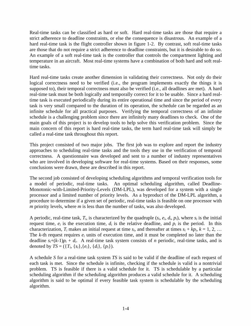
Real-time tasks can be classified as hard or soft. Hard real-time tasks are those that require a strict adherence to deadline constraints, or else the consequence is disastrous. An example of a hard real-time task is the flight controller shown in figure 1-2. By contrast, soft real-time tasks are those that do not require a strict adherence to deadline constraints, but it is desirable to do so. An example of a soft real-time task is the controller that controls the compartment lighting and temperature in an aircraft. Most real-time systems have a combination of both hard and soft real-time tasks.

Hard real-time tasks create another dimension in validating their correctness. Not only do their logical correctness need to be verified (i.e., the program implements exactly the things it is supposed to), their temporal correctness must also be verified (i.e., all deadlines are met). A hard real-time task must be both logically and temporally correct for it to be usable. Since a hard real-time task is executed periodically during its entire operational time and since the period of every task is very small compared to the duration of its operation, the schedule can be regarded as an infinite schedule for all practical purposes. Verifying the temporal correctness of an infinite schedule is a challenging problem since there are infinitely many deadlines to check. One of the main goals of this project is to develop tools to help solve this verification problem. Since the main concern of this report is hard real-time tasks, the term hard real-time task will simply be called a real-time task throughout this report.

This project consisted of two major jobs. The first job was to explore and report the industry approaches to scheduling real-time tasks and the tools they use in the verification of temporal correctness. A questionnaire was developed and sent to a number of industry representatives who are involved in developing software for real-time systems. Based on their responses, some conclusions were drawn, these are described in this report.

The second job consisted of developing scheduling algorithms and temporal verification tools for a model of periodic, real-time tasks. An optimal scheduling algorithm, called Deadline-Monotonic-with-Limited-Priority-Levels (DM-LPL), was developed for a system with a single processor and a limited number of priority levels. As a byproduct of the DM-LPL algorithm, a procedure to determine if a given set of periodic, real-time tasks is feasible on one processor with m priority levels, where m is less than the number of tasks, was also developed. A periodic, real-time task, Ti, is characterized by the quadruple (si, ei, di, pi), where si is the initial request time, ei is the execution time, di is the relative deadline, and pi is the period. In this characterization, Ti makes an initial request at time si, and thereafter at times si + kpi, k = 1, 2, … The k-th request requires ei units of execution time, and it must be completed no later than the deadline si+(k-1)pi + di. A real-time task system consists of n periodic, real-time tasks, and is denoted by TS = ({Ti, {si},{ei}, {di}, {pi}). A schedule S for a real-time task system TS is said to be valid if the deadline of each request of each task is met. Since the schedule is infinite, checking if the schedule is valid is a nontrivial problem. TS is feasible if there is a valid schedule for it. TS is schedulable by a particular scheduling algorithm if the scheduling algorithm produces a valid schedule for it. A scheduling algorithm is said to be optimal if every feasible task system is schedulable by the scheduling algorithm.

1-4

1.2 REPORT OVERVIEW.

This report begins with a summary of the industry survey results. Three approaches that have been used to schedule a real-time task system are (1) Clock-Driven, (2) Processor-Sharing, and (3) Priority-Driven. It was reasoned that the Priority-Driven approach was far superior to the Clock-Driven and Processor-Sharing approaches. The report then reviews the literature on Priority-Driven scheduling algorithms, which can be divided into two categories: Dynamic-Priority and Fixed-Priority. While Dynamic-Priority scheduling algorithms are more effective than Fixed-Priority scheduling algorithms, they are rarely used in practice because of the overhead involved. Therefore, the report concentrates on Fixed-Priority scheduling algorithms. The remaining portions of the report focus on specific scheduling model. Leung and Whitehead have shown that the Deadline Monotonic algorithm is an optimal Fixed-Priority scheduling algorithm for one processor. Unfortunately, the algorithm assumes that the number of priorities is the same as the number of real-time tasks. In practice, one can only have a limited number of priorities, say m, supported by a system. Under this scenario, the Deadline Monotonic (DM) algorithm fails to be optimal, and the optimal scheduling algorithm DM-LPL was developed, along with a separate procedure to check if a given set of real-time tasks is feasible on one processor with m priority levels. The same problem is explored for multiprocessor systems. It is demonstrated that finding an optimal assignment is strongly nondeterministic polynomial (NP)-hard, which is tantamount to showing that there is no efficient algorithm to solve this problem. A problem Q is NP-hard if all problems in the NP-class are reducible to Q. Motivated by the computational complexity, several heuristics for solving this problem are suggested. The minimum processor utilization, U(n), for a set of n unit-execution-time tasks is also studied. U(n) is the threshold for the total processor utilization of the n tasks, below which they are always schedulable. It is conjectured that 1 1 1 1 1

1 1 2 3( ) ...n n n nU n − + −= + + + + + 2n Some special cases of this conjecture are proven, but time was not available to perform the complete proof. Some other tasks were planned for this research effort (i.e., study of fault-tolerant issues, which are concerned with schedulability analysis when there are time losses due to transient hardware or software failures, and study of central processing unit (CPU) scheduling coupled with input/output (I/O) activities). However, due to time constraints, significant progress was not made in these areas. These remain topics to be considered in future research. 1.3 USING THIS REPORT.

There are a number of potential uses for this report. Since this research task falls more into the category of basic research than many of the Federal Aviation Administration (FAA) Software and Digital System Safety Project research and development initiatives, some explanation of

1-5

how various readers may use the report is provided. The intended audience for this report is certification authorities, industry representatives, and researchers. A brief summary of how each audience can use this report is listed below. • Certification Authorities. Certification authorities will primarily benefit from the

summary of the industry survey, the tutorial of the different scheduling approaches, and the research results (sections 2, 3, and 5). Additionally, certification authorities might desire to browse section 4 and appendix B for information purposes, realizing that these sections are research-focused and will require significant work before they can be implemented in an actual aircraft project.

• Industry Representative. The industry can benefit from this entire report but should

realize that section 4 and appendix B are at a research stage. The proofs will require verification by a qualified independent entity before they can be implemented in an actual aviation project. It is also likely that the industry would need to develop tools to help implement the algorithms of this report into a usable format.

• Researchers. As mentioned before and discussed throughout this report, this research

effort is really the beginning of what needs to be done before implementing the algorithms. Researchers will likely benefit most from section 4 and appendix B, and will likely want to build upon these in additional work. Section 5 provides specific information about where the future research needs to go.

1-6

2. SURVEY OF INDUSTRY APPROACHES.

A Real-Time Scheduling Analysis (RTSA) Questionnaire was sent out to industry representatives who are involved in developing software for real-time systems. The questionnaire is shown in appendix A. Fifteen questionnaires were returned and are tabulated in appendix A.

Of the 15 respondents, the majority (12) of them work for avionics or engine control developers or aircraft or engine manufacturers. The majority either verify/test real-time scheduling performance, perform RTSA on aviation system projects, or develop real-time operating systems (RTOS) that support RTSA. On the whole, the respondents had the appropriate background to answer this questionnaire. The responses and questions are summarized below. Question A.2.1 asked, “What type of events are typically used to trigger time-critical functions of your real-time system (e.g., interrupts, data message queries, data refresh rates, (pilot) user input, change of state, certain conditions, display refresh rates, etc.)?” Interrupts were mentioned by ten respondents as the main events that are typically used to trigger the time-critical functions of their real-time systems. This fits well with the DM algorithm, which is essentially interrupt-driven. Question A.2.2 asked, “What are typical performance requirements that your real-time system must meet?” The majority of the respondents mentioned that critical tasks must meet hard real-time deadline constraints. The response times mentioned are from a few milliseconds to hundreds of milliseconds. This justifies the study of scheduling analysis of hard real-time tasks, which is the main topic in this project. Question A.2.3 asked, “Where are your performance requirements for time-critical functions typically defined (e.g., system requirements or interface control documents, software requirements document)?” System requirements, interface requirements, and software requirements are the most popular responses. It appears that performance requirements for time-critical functions are typically defined in those documents. Question A.2.4 asked, “How do you distinguish time-critical functions from other functions in your application?” The majority of the respondents answer that time-critical functions are explicitly stated in the requirement. Question A.2.5 asked, “Do your time-critical functions have dependencies on hardware or shared hardware devices (central processing unit, memory, data buses, I/O ports, queues, etc.) with other software functions of your application or other applications resident in the system? If yes, please explain.” The answers were mixed. Some say that there are no dependencies, while others say that there are. The results are inconclusive. Question A.2.6 asked, “What are some mechanisms that your application (software and hardware) uses to ensure that “time-critical triggers” get handled at the appropriate priority and gain the relevant resources to ensure that your performance requirements are achieved?” Priority levels assigned to interrupts were mentioned by several people as the mechanism used to

2-1

schedule time-critical tasks. Some people mentioned that the computers they use have only one priority level, such as the PowerPC. This fits well with the model that the system has a limited number (m) of priority levels (as proposed for this research project). In this case, m = 1. Question A.2.7 asked, “What type of reviews, analyses and testing does your team use to ensure that time-critical functions will satisfy their performance requirements, especially in worst-case condition scenarios?” The majority of respondents mentioned that they can obtain worst-case execution time by analyzing the code. As for validation, most respondents use emulator or some ad hoc approach to test. This is risky because an emulator can only show that it will work most of the time. It does not show that it will work all of the time. There is a definite need for a formal validation procedure which gives a guarantee that it will work all the time. Question A.3.1 asked, “What approaches to message passing have your projects utilized?” The answers are so different that it was difficult to draw any conclusions. It seems that message passing mechanism is a function of the hardware and operating systems used by the organization. This explains the diverse answers. Question A.3.2 asked, “Do your messages communicate with each other? If yes, please explain how.” The majority answered that messages do not communicate with each other. Question A.4.1 asked, “What type of processors have you used for your systems?” The majority of respondents currently use Intel processors; however, PowerPC seems to be gaining momentum. A small number of respondents use Motorola or TI chips. By far, the largest number use Intel family of processors. Question A.4.2 asked, “Have you found any peculiarities with any of the processors that affect the real-time scheduling analysis? If yes, please explain the peculiarities and how they were addressed.” The answers to this question varied significantly. Some pointed out that the lack of multiple interrupt priorities in PowerPC makes it difficult to schedule real-time tasks. This confirms the hypothesis of this research effort that more priority levels make scheduling easier. Some mentioned that the cache memory makes it difficult to analyze the worst-case running time, since the execution time depends on the hit ratio of the cache. Some mentioned that the pipeline processor also makes it difficult to estimate the worst-case running time. Question A.4.3 asked, “Do your systems use a single processor or multiple processors? If multiple processors, how is the system functionality distributed and handled across processors?” Nine respondents said that they use a single processor while six respondents said that they use multiple processors. One respondent mentioned that they use both single and multiple processors. It seems that they are about evenly divided, with the single processor having a slight edge. Question A.5.1 asked, “What scheduling algorithms/approaches have you used to schedule your system tasks at run time? Please match the algorithm (e.g., preemptive priority, round robin, etc.) with the system type (e.g., display, communication, navigation, etc.).” The majority responded that they use pre-emptive priority scheduling algorithm, of which the DM algorithm is a member. One respondent mentioned that they use Rate Monotonic (RM) Analysis.

2-2

Question A.5.2 asked, “If you used priority scheduling, how many priorities levels were assigned? How was priority inversion avoided? How did the number of priority levels compare to the number of processes?” The majority of the respondents said that they used 3 to 20 levels. One can conclude that the number of priority levels is relatively small, compared to the number of real-time tasks in the system. Question A.5.3 asked, “What kind of scheduling problems have you encountered in multitasking systems and how were they addressed?” A fair number of respondents did not comment on this question. Therefore, it was not possible to draw any valid conclusions. Question A.5.4 asked, “Have you used real-time operating systems to support your schedule guarantees? If yes, what kind of operating systems have you used and what kind of scheduling challenges have you encountered?” Most respondents said that they did not use real-time operating systems to support their schedule guarantees. For the few who said they did, they used in-house proprietary systems. It seems that there is a learning curve here. If the tools are made available to them free of charge, they may in fact use these tools in the future. Question A.5.5 asked, “Do you verify what data gets dumped, due to priority settings and functions getting preempted? If yes, how does it affect your system?” Most respondents replied No or N/A. Therefore, there was insufficient data to draw any conclusions. Question A.5.6 asked, “Do you use tools to assist in the real-time scheduling analysis? If yes, what kind of tools? How are the outputs of these tools verified?” Most respondents replied No or that they use emulators and simulators. This can create problems since these are not rigorous and formal analyses. Question A.5.7 asked, “What trends in commercial aviation systems do you think will challenge the current scheduling approaches (i.e., may lead to the need for new scheduling algorithms)?” Some said that multiple thread real-time deadline scheduling analysis will be the future trends that challenge the current scheduling approaches. Some said that the desire to reuse, the desire to inherit confidence from reuse, and the desire to use nondevelopmental items will be the major challenges to the current scheduling approaches. These comments point to the importance of a theory of scheduling on multiple processors. Question A.6.1 asked, “After system development, do you verify that deadlines are met and scheduling analysis assumptions are correct? If yes, please explain how.” The majority of the respondents said that they verified that deadlines are met and scheduling analysis assumptions are correct after system development. Question A.6.2 asked, “In what areas of timing verification or validation have you encountered problems and how were they addressed?” The answers were so diverse that it was difficult to draw any conclusions. It seems that the problems encountered is highly dependent on the specific problems and the hardware or software used in the company. Question A.7.1 asked, “Does your testing allow for faults? If yes, please explain.” Most respondents said that their testing allow for faults. This is mostly handled by injecting faults into

2-3

the system and checking to see how the system responds to the faults. Responses indicated that no worst-case analysis is done; i.e., it is mostly done in an ad hoc manner. Question A.8.1 asked, “In your opinion, what are the major issues regarding RTSA and its verification?” Responses varied significantly and are summarized below. • Confirmation of timing issues under all foreseeable circumstances is a major issue

regarding RTSA and its verification.

• Testing is difficult when modifications and/or changes are made.

• The tools are very expensive and not always available.

• The analysis tends to be intuitive and lacks formal analysis.

• The operating systems are so general that they are of little use in dealing with real-time systems.

From the responses of the questionnaire, the following conclusions were drawn: • There is a need for scheduling analysis and verification in the avionics industry.

• The current practice is by ad hoc methods. Tools are seldom used either because they are expensive and not available, or the operating systems are for general purpose and not usable for real-time systems.

• The trend is towards multiprocessor systems.

• Software developers do test for fault tolerance, but the main method used is by means of fault injection which is rather ad hoc.

It was concluded that developing defined approaches and algorithms for scheduling, deadline verification, and fault tolerance will significantly help the avionics industry. Furthermore, these theories should be implemented into a software tool suite that can be made available to anyone who desires to use it. As more and more people use these tools (which may need to be qualified), future systems will be less error-prone and easy to maintain and modify.

2-4

3. TUTORIAL ON DIFFERENT SCHEDULING APPROACHES.

Whether a set of real-time tasks can meet all their deadlines depends on the characteristics of the tasks (e.g., periods and execution times) and the scheduling algorithms used. Scheduling algorithms can be classified as pre-emptive and non-pre-emptive. In non-pre-emptive scheduling, a task once started must be executed to completion without any interruptions. By contrast, pre-emptive scheduling permits suspension of a task before it completes, to allow for execution of another more critical task. The suspended task can resume execution later on from the point of suspension. While pre-emptive scheduling incurs more system overhead (e.g., context switching time due to pre-emptions) than non-pre-emptive scheduling, it has the advantage that processor utilization (the percentage time that the processor is executing tasks) is significantly higher than non-pre-emptive scheduling. For this reason, most of the scheduling algorithms presented in the literature are pre-emptive scheduling algorithms. There are three major approaches in designing pre-emptive scheduling algorithms for real-time tasks: Clock-Driven, Processor-Sharing, and Priority-Driven. Each approach is described below. The Clock-Driven approach is the oldest method used to schedule real-time tasks. In this method, a schedule is handcrafted and stored in memory before the system is put in operation. At run time, tasks are scheduled according to the scheduling table. After the scheduler dispatches a task, it will set the hardware timer to generate an interrupt at the next task switching time. The scheduler will then go to sleep until the timer expires. This process is repeated throughout the whole operation. The Clock-Driven approach has several disadvantages that render it undesirable to use: (1) it requires a fair amount of memory to store the scheduling table; (2) a slight change in task parameters (e.g., execution time and period) requires a complete change of the scheduling table, which can be very time-consuming, and (3) this approach is not adaptive to any change at run time. For example, if a system fault occurs or a task runs for less (or more) time than predicted, it is not clear how the scheduling decisions can be adapted to respond to the change. The Processor-Sharing approach is to assign a fraction of a processor to each task, depending on the utilization factor (execution time divided by period) of the task. Since a processor cannot be used by more than one task at the same time, the processor sharing is approximated by dividing a time interval into smaller time slices and giving each task an amount proportional to the fraction of processor assigned to the task. For example, if a task is assigned 0.35 of a processor, then the task would receive 35 percent of the time slices in the time interval. The time slice has to be made very small to obtain a close approximation of processor sharing. But when the time slice is very small, a significant amount of time will be spent in context switching. This is a major drawback of the Processor-Sharing approach. In the Priority-Driven approach, each task is assigned a priority. At run time, the ready task that has the highest priority will receive the processor for execution. Priorities can be assigned at run time (Dynamic-Priority) or fixed at the beginning before the operation starts (Fixed-Priority). Fixed-Priority scheduling algorithms incur far less system overhead (context switching time)

3-1

than Dynamic-Priority scheduling algorithms, since the scheduler does not need to determine the priority of a task at run time. Furthermore, Fixed-Priority scheduling algorithms can be implemented at the hardware level by attaching the priority of a task to the hardware interrupt level. On the other hand, processor utilization under Fixed-Priority scheduling algorithms is usually not as high as Dynamic-Priority scheduling algorithms. It is known that Fixed-Priority scheduling algorithms may yield a processor utilization as low as 70 percent, while Dynamic-Priority scheduling algorithms may yield a processor utilization as high as 100 percent. One of the most well-known Dynamic-Priority scheduling algorithm is the Earliest-Deadline-First (EDF) algorithm, which assigns the highest priority to the task whose deadline is closest to the current time. It is known that EDF is optimal for one processor [2 and 3], in the sense that any set of tasks that can be feasibly scheduled by any Dynamic-Priority scheduling algorithms can also be feasibly scheduled by EDF. However, EDF is not optimal for two or more processors [4]. At the present time, no scheduling algorithm is known to be optimal for two or more processors. The two most well known Fixed-Priority scheduling algorithms are the Rate-Monotonic (RM) and Deadline-Monotonic (DM) algorithms [3 and 5]. RM assigns the highest priority to the task with the smallest period (or equivalently, the highest request rate), while DM assigns the highest priority to the task with the smallest relative deadline. It should be noted that DM and RM are identical if the relative deadline of each task is identical to its period. Leung and Whitehead [5] have shown that DM is optimal for one processor, in the sense that any set of tasks that can be feasibly scheduled by any Fixed-Priority scheduling algorithms can also be feasibly scheduled by DM. Liu and Layland [3] have shown that RM is optimal when the relative deadline of each task coincides with its period; it fails to be optimal if the deadline of some task is not identical to its period. Both DM and RM fail to be optimal for two or more processors [6]. At the present time, no scheduling algorithm is known to be optimal for two or more processors. The following documents are specifically recommended to further describe the scheduling approaches, and also see references 1-6.

• S. Natarajan, ed., (1995), Imprecise and Approximate Computation, Kluwer, Boston.

• A.M. Van Tilborg and G.M. Koob, eds., Foundations of Real-Time Computing: Scheduling and Resources Management, Kluwer, Boston.

3-2

4. DESCRIPTION OF SCHEDULING MODEL.

The research topics in this project were planned to be (1) priority assignment, (2) multiprocessor scheduling, (3) fault tolerant issue, and (4) I/O activities. However, because of time limitations, only the first two topics were studied. In this report, the scheduling model for the first two topics is defined. A periodic, real-time task, Ti, is characterized by a quadruple (si, ei, di, and pi), where si is the initial request time, ei is the execution time, di is the relative deadline, and pi is the period. In this characterization, Ti makes an initial request at time si, and thereafter at times si + kpi, k = 1, 2, . . . The kth request requires ei units of execution time and it must be completed no later than the deadline si + (k-1)pi + di. A real-time task system consists of n periodic, real-time tasks, and is denoted by TS = ({ Ti } , { si } , { ei } , { di } , { pi }). A schedule S for a real-time task system TS is said to be valid if the deadline of each request of each task is met. Since the schedule is infinite, checking if the schedule is valid is a non-trivial problem. TS is said to be feasible if there is a valid schedule for it. TS is said to be schedulable by a particular scheduling algorithm if the scheduling algorithm produces a valid schedule for it. A scheduling algorithm is said to be optimal if every feasible task system is schedulable by the scheduling algorithm. With respect to the above model, there are several important questions whose answers are essential in validating the temporal correctness of a real-time task system. First, how does one determine if a real-time task system is feasible? Second, how does one determine if a real-time task system is schedulable by a particular scheduling algorithm? Third, what are the optimal scheduling algorithms? By definition, a real-time task system is feasible if and only if it is schedulable by an optimal scheduling algorithm. Thus, these three questions are interrelated. There are several important assumptions associated with this model. First, ei is assumed to be the maximum execution time required by Ti. At run time, it is assumed that Ti never requires more than ei units of execution time at each request, although it could use less time. Second, it is assumed that context switching time is negligible. If this is not a valid assumption, ei must be adjusted to account for the time loss due to context switching. Third, the minimum time lapse between two consecutive requests of Ti is pi. At run time, the time lapse between two consecutive requests is at least pi; it could be more than pi, but not less. Fourth, the relative deadline of each request is di. At run time, the relative deadline of each request can be longer than di but not shorter. These assumptions must be strictly adhered to in order for the theory to work.

4-1/4-2

5. RESULTS AND FUTURE WORK.

5.1 RESULTS.

This project consisted of two major jobs. The first job was to explore and report the industry approaches to scheduling real-time tasks and the tools they use in the verification of temporal correctness. A questionnaire was developed and sent to a number of industry representatives who were involved in developing software for real-time systems. From the responses of the questionnaire, the following conclusions can be drawn: • There is a need for scheduling analysis and verification in the avionics industry.

• The current practice is by ad hoc methods. Tools are seldom used either because they are expensive and not available, or the operating systems are for general purpose and not usable for real-time systems.

• The trend is towards multiprocessor systems.

• Software developers do test for fault tolerance, but the main method used is by means of fault injection which is rather ad hoc.

It was concluded that developing defined approaches and algorithms for scheduling, deadline verification, and fault tolerance will significantly help the avionics industry. Furthermore, these theories should be implemented into a software tool suite that can be made available to anyone who desires to use it. As more and more people use these tools (which may need to be qualified), future systems will be less error-prone and easy to maintain and modify. The second job consisted of developing scheduling algorithms and temporal verification tools for a model of periodic, real-time tasks. The report began with a discussion of the three approaches that have been used to schedule a real-time task system: (1) Clock-Driven, (2) Processor-Sharing, and (3) Priority-Driven. It was reasoned that the Priority-Driven approach is far superior to the Clock-Driven and Processor-Sharing approaches. The report then reviewed the literature on Priority-Driven scheduling algorithms, which can be divided into two categories: Dynamic-Priority and Fixed-Priority. While Dynamic-Priority scheduling algorithms are more effective than Fixed-Priority scheduling algorithms, they are rarely used in practice because of the overhead involved. Therefore, the report concentrated on Fixed-Priority scheduling algorithms. Priority-Driven scheduling is probably the most appropriate approach in scheduling periodic, real-time tasks. In this project, Fixed-Priority scheduling algorithms for computing systems with limited priority levels were studied. A procedure to test if a given priority assignment is valid (i.e., all deadlines are met) was developed. Furthermore, an optimal priority assignment algorithm, DM-LPL, for one processor was given. The algorithm was implemented using the C language and is shown in appendix C.

5-1

For multiprocessors, the problem of finding the minimum number of processors with m priority levels to schedule a set of tasks was shown to be NP-hard. Two heuristics were provided, FF and FFDU, for this problem. The special delivery case where each task’s execution time is one unit was also considered. Under this model, an attempt was made to develop a utilization threshold, U(n), below which a set of n tasks is always schedulable. For the unlimited priority levels, it was

conjectured that 2 3

1 12

1( )

n

ii n

U n−

= −

⎛ ⎞= +⎜ ⎟⎝ ⎠∑ n , which is better than the bound of given by Liu

and Layland [3]. This conjecture was proved for two special cases.

1/(2 1)nn −

5.2 FUTURE WORK.

There are four areas where future work should be performed: • Develop a full proof of the conjecture started in this report.

− The special case when d1 and d2 are arbitrary has been proved. It remains to be

shown that the conjecture is valid when d3, d4, …, dn-1 are also arbitrary. • Perform an independent verification of the algorithms in the report, as well as a

verification of the full proof.

− The results obtained in this report should be reviewed by an independent expert in scheduling theory.

• Perform a study of fault-tolerant issues, which are concerned with schedulability analysis

when there are time losses due to transient hardware/software failures.

− A major issue in this area is to characterize the worst-case scenario due to time losses.

• Perform a study of central processing unit (CPU) scheduling coupled with input/output

(I/O) activities.

− The main issue in this area is to couple pre-emptive scheduling (CPU scheduling) with non-pre-emptive scheduling (I/O activities).

5-2

6. REFERENCES.

1. Liu, J.W.S., Real-Time Systems, Prentice Hall, New Jersey, 2000.

2. Labetoulle, J., “Some Theorems on Real-Time Scheduling,” in Computer Architecture and Networks, E. Gelenbe and R. Mahl, eds., North-Holland, Amsterdam, 1974.

3. Liu, C.L., and Layland, J.W., “Scheduling Algorithms for Multiprogramming in a Hard Real-Time Environment,” J. of ACM, Vol. 20, 1973, pp. 46-61.

4. Leung, J.Y-T., “A New Algorithm for Scheduling Periodic, Real-Time Tasks,” Algorithmica, Vol. 4, 1989, pp. 209-219.

5. Leung, J.Y-T. and Whitehead, J., “On the Complexity of Fixed-Priority Scheduling of Periodic, Real-Time Tasks,” Performance Evaluation, Vol. 2, 1982, pp. 237-250.

6. Dhall, S.K. and Liu, C.L., “On a Real-Time Scheduling Problem,” Operations Research, Vol. 26, 1978, pp. 127-140.

6-1/6-2

APPENDIX A—INDUSTRY SURVEY AND RESPONSES The following is the Real-Time Scheduling Analysis (RTSA) Questionnaire Analysis A.1 BACKGROUND QUESTION. A.1.1 BACKGROUND QUESTION #1. What kind of organization do you work for?

Avionics or engine control developer Aircraft or engine manufacturer Communications, navigation, or surveillance system developer for air traffic

management Software tool developer Third party software developer (e.g., operating system or library) Consultant Federal Aviation Administration Other government agency (please specify): ___________________ Other, (please specify):

________________________________________________________ Of the 15 surveys responding, the breakdown was as follows:

8 Avionics or engine control developer 4 Aircraft or engine manufacturers 1 Software tool developer 1 Consultant

1 Other, (please specify): Software Verification Co.

A.1.2 BACKGROUND QUESTION #2.

What is your role relevant to RTSA? (Check all that apply) I perform RTSA on aviation system projects I develop real-time operating systems (RTOS) that support RTSA I use tools to perform RTSA I verify/test real-time scheduling performance I am an FAA engineer who approves compliance to DO-178B I am a Designated Engineering Representative (DER) who approves compliance to

DO-178B Other, (please specify):

Of the 16 surveys responding, with many individuals responsible for more than one role, the breakdown was as follows:.

6 I perform RTSA on aviation system projects 2 I use tools to perform RTSA 9 I verify/test real-time scheduling performance

A-1

5 I am a Designated Engineering Representative (DER) who approves compliance To DO-178B

A.2 REAL-TIME SYSTEM DEVELOPMENT. A.2.1 REAL-TIME SYSTEM DEVELOPMENT QUESTION A. What type of events are typically used to trigger time-critical functions of your real-time systems (e.g., interrupts, data message queries, data refresh rates, (pilot) user input, change of state, certain conditions, display refresh rates, etc.)? Of the 15 surveys responding, their answers were as follows: 1. Combination of fixed schedule (i.e., clock time) plus certain conditions (for example,

tracked signal weakness switches mode from tracking to acquisition) 2. Data inputs, data refresh rates, data queries, display refresh rates 3. In the OS all of the above are supported 4. Elapsed time, message update due 5. Interrupts 6. Interrupts, RTOS messages, RTOS semaphores or other similar mechanisms. 7. Fixed time interval scheduling interrupts only 8. RTSA is interrupt driven by time-to-go counters. We use an executive routine to

establish priorities. Our Run Time Executive was written In-house. 9. Interrupts and change of state 10. Table driven scheduler based upon statically built table by an external, qualified tool.

The table contains information regarding I/O timing (when to send data and when to read data), as well as process scheduling information

11. Time-based interrupts 12. Hardware interrupts, sensor/hardware inputs, airframe computer inputs, etc 13. Typically we use interrupts. In some instances it is an external input, such as incoming

data, from another device that causes an interrupt to be generated. 14. Incoming data messages (interrupt or polled), timer expiration, user input (Key press,

toggle switch, etc), sensor state change (interrupts or polled).

A-2

15. Interrupts are used for the initiation of the real-time processing. Analysis of Question A Real-Time System Development Interrupts were mentioned by 10 respondents as the main events that are typically used to trigger time-critical functions of their real-time systems. A.2.2 REAL-TIME SYSTEM DEVELOPMENT QUESTION B. What are typical performance requirements that your real-time system must meet? Of the 15 surveys responding, their answers were as follows: 1. There are hardware and software deadlines. For the software, three independent bits need

to be assembled and delivered every 0.6 microseconds. 2. Some requirements need to meet millisecond response times/tolerances; others have

multiple second responses with millisecond tolerances. 3. The clock ticks at 1 kHz. All scheduling operations are driven by the ‘ticking clock’.

User ‘frame’ times are typically 40-80 Hz 4. Servo loop closure without overshoot or significant lag. Service data bus and access

information from the data bus according to schedule. Determine fault state based on successive out of range input for time frame.

5. Critical task must meet their real-time dead-line scheduled activities. 6. Sample rates in excess of 50 Hhz. For DSP applications. Multiple 8 KHz. Sample rate

audio channels. 7. Level A assurance that all functions are completed before the next interrupt. 8. Max min limits on input/output events, gain phase margin on control loops, iteration rates

and transport delay times on selected functions 9. Throughput margins of 50% were required by government contract. There were similar

hardware reserve margin requirements on memory and I/O 10. There is a 1 KHz interrupt and several I/O devices interrupt 11. All aircraft I/O includes transmission and jitter requirements. Typical data rates range

from 1 Hz to 80 Hz. 12. 80 Hz update rate

A-3

13. The hardware/computer shall operate without adverse affect on the engine or aircraft, such as lost of engine thrust, adverse increase or decrease of engine thrust or cause in-flight shut down.

14. As a military application our performance requirements are mainly based off of our 1553

bus rates. Thus we have certain message rates that our system must maintain for example rates of 50Hz or 25Hz etc. In addition – we may interface to an external device that requires data to be transferred to it within a few milliseconds after the data has changed.

15. Digital signal processing incoming data rate (radio IF): 200 ksam

Radio push-to-talk to RF on: < 50 ms; user input to display update: < 100 m Sensor change to display update: < 100 ms

16. Performance requirements that are most critical include the time that the system detects

an engine threshold exceedance (such as overspeed; under speed; excessive engine temperature; etc.) until the fuel flow is terminated to shut the engine down. This is usually on the order of a few milliseconds.

A.2.3 REAL-TIME SYSTEM DEVELOPMENT QUESTION C. Where are your performance requirements for time-critical functions typically defined? (e.g., system requirements or interface control documents, software requirements document) Of the 15 surveys responding, their answers were as follows:

1. System requirements and interface requirements 2. Time critical requirements may show up in our system requirements, software

requirements or software design (low level requirements) 3. System requirements 4. Software Requirements Document 5. Software requirements Documents 6. System requirements, interface control documents, software requirements document 7. All the above 8. Ours were specified by government contract- typically some version of the TADSTAND 9. Through system design analysis or from similarity to previous systems, we can usually

distinguish time-critical functions.

A-4

10. System requirements and interface control documents. On occasion, lower level performance requirements may appear in the software requirements document. Hardware documents also contain performance requirements as they pertain to the support of the I/O and O/S.

11. Systems requirements 12. Interface control document, computer hardware operation requirements and software

requirement documents 13. Critical time with max latencies would be defined in our System and Sub-System

Specification (i.e., our system requirements) document. 1553 message rates would be defined in our Interface Control Documents and some timing would be documented in our Software Requirements.

14. For inter-process communications timing. System requirements for input to output

timings and user interface performance, software requirement 15. These are typically defined in the software requirements document- with some being

defined in the system requirements document. A.2.4 REAL-TIME SYSTEM DEVELOPMENT QUESTION D.

How do you distinguish time-critical functions from other functions in your application? Of the 15 surveys responding, their answers were as follows: 1. All requirements must be met eventually. Some deadlines are obviously easy to meet;

others will require some effort and/or have some risk associated with them. Perhaps it would be helpful to imagine all requirements having a deadline to be filled in, and if a recipient of an item (data, for example) really doesn’t care by when something is accomplished, they should say so. NASA/JPL sometimes uses a time constraint network, where timing is stated with respect to other events, rather than with respect to time deadlines. For example, some aspects of a flight might not be required to be delivered until the flight arrives at the gate.

2. By the time element of the requirement (i.e., must respond within 200 mS, or must do x

after y +/- z seconds. 3. Time critical information is embedded in the requirement 4. Error reporting has a unique identifier for each malfunction 5. By creating software or system requirements specifying the timing 6. Badly

A-5

7. I believe your question refers to arbitration done by the Executive. Levels of priority were established and the Executive routine carried them out. Priorities were established during the software design phase following analysis of the requirements.

8. Through system design analysis or from similarity to previous systems, we can usually

distinguish time-critical functions. 9. From an O/S perspective, all functions are time critical. That is, they have specific

timing constraints placed upon them that must be honored. The determination of who is “more time critical” than others is a system architecture exercise.

10. We don’t 11. We don’t 12. Time-critical functions would be documented as such 13. Listed in software design description, notation in function comment header 14. All functions in the application are time-driven and are treated as time-critical- with the

exception of the low-level transmission and reception of serial data. This serial communication is interrupt-driven and will be serviced when data is available from the host computer to which the electronic control unit is communicating or when new data needs to be sent to the host computer. The processing and responding to complete messages in the system is also time-driven (a determination is made for whether a completed message has been received that needs to be acted on). Consequently, distinguishing from the time-critical functions and those that are not time-critical is done by dedicating separate memory resources to the serial.

A.2.5 REAL-TIME SYSTEM DEVELOPMENT QUESTION E. Do your time-critical functions have dependencies on hardware or shared hardware devices (central processing unit, memory, data buses, I/O ports, queues, etc.) with other software functions of your application or other applications resident in the system? If yes, please explain. Of the 15 surveys responding, their answers were as follows: 1. Multiple software entities can be incomplete at one time; knowledge about which ones

are incomplete is used in deciding which entities get resource use assigned to them. 2. Sometimes, might have multi-processor system that must meet data bus timing protocol.

Might be a hardware event that triggers the start of a time critical function. 3. The application has a dependency on the RTOS. The RTOS has a dependency on the

system and applications, e.g. cache usage, memory configurations (coherent or non-coherent etc).

A-6

4. No 5. Yes. A system clock (counter/timer) is used for all software related timing functions.

The RTS owns the system clock. A hardware watch dog is also used, which must be updated on a periodic basis

6. Yes, A/Ds and D/As for RF and audio sampling 7. No 8. It depends- hardware limitations that were known were part of the design. These

dependencies were usually noted in the System and/or Software Requirements Specification. They were occasionally “discovered” during the Requirements Analysis phase- at great embarrassment.

9. Yes. Generally the interrupt servicing functions must share hardware devices and

memory with other applications. 10. Typically the answer is yes, when looking at I/O hardware devices. However, our

hardware designers use queues, state machines and other methods to abstract as much timing critical “stuff” away from the software, as possible.

11. No 12. Yes. There is memory loader software that is activated only when certain hardware and

software conditions are set. 13. Yes, we must receive data from one subsystem and within a specified amount of time

pass the information onto another subsystem – in some case using the input data to calculate the data that is to be output.

14. Time-critical functions typically share CPU, memory and other resources with other

functions 15. Yes, the time-critical functions do have hardware dependencies on I/O devices. A.2.6 REAL-TIME SYSTEM DEVELOPMENT QUESTION F. What are some mechanisms that your application (software and hardware) uses to ensure that “time-critical triggers” get handled at the appropriate priority and gain the relevant resources to ensure that your performance requirements are achieved? Of the 15 surveys responding, their answers were as follows:

A-7

1. A look-up table is provided (all at once) with input describing the tasks currently incomplete. The content of the look-up table tells which software task is to receive the processing resources next.

2. We don’t use RTOS, so we write software to achieve desired responses (when possible). 3. Interrupt locking is used, OS/kernel locking, semaphores and priority inheritance, work

queues for work deferrals, etc. 4. High Interrupt priority, also time critical code has hard vectors to interrupt service

routines that cannot be modified by a run time operation. We are concerned about software maintenance activities adding new priority sets with higher priorities for less important processes. We document heavily the priority rationale.

5. Task priorities and interrupt priorities. 6. They are given the highest priority level within the RTOS. Or else they are handled

outside of the RTOS with independent interrupts 7. By restricting to the one interrupt, and insisting on completion of time critical tasks. 8. Careful Integration testing and thorough V&V was our preferred path. Demonstration,

analysis, whatever was appropriate. 9. Interrupt and task priorities are assigned appropriate values 10. All resources are defined statically at build time by a qualified tool. Processes are

assigned specific resources. This ensures the resources will be ready when needed, and permits the O/S to detect any resource usage violations (i.e., partitioning violations).

11. Check on process completion and hardware watchdog 12. Our software uses watch dog monitor and certain CPU interrupt handlers. 13. As we use a PowerPC with only one external interrupt the “time critical” issues have to

be designed into the system. There is NO way to prioritize interrupts in our system so the top level design must take this issue into account. Software must ensure all interrupt handlers are as quick as possible.

14. Hardware timers, prioritized hardware and software interrupts, pre-emptable and

prioritized tasks. No (or very low iteration count) loops in round-robin systems.

15. There are no priority mechanisms in an interrupt occurs at a pre-defined interval and this

initiates real-time processing. The software verifies that the processing from the previous interval has completed. If it has not, the first time the anomaly occurs, it is simply

A-8

recorded and processing for the next interval is initiated directly after the completion of the tasks from the previous interval. If two such overruns occur in a row, then the application simply executes an infinite loop, which will cause the engine to shut down. In addition, there is a hardware watchdog discrete output that needs to get strobed each interval. If the watchdog is NOT strobed during each interval, then the hardware will cause the engine to shut down our software.

A.2.7 REAL-TIME SYSTEM DEVELOPMENT QUESTION G. What type of reviews, analyses and testing does your team use to ensure that time-critical functions will satisfy their performance requirements, especially in worst-case condition scenarios? Of the 15 surveys responding, their answers were as follows: 1. We know the instructions and the instruction execution times. 2. Worst case timing analysis, overloaded resource tests 3. Need a two day essay to answer this.

In the past we analyzed the paths of the RTOS and determined what the relationship to time was with inputs. Things have got a lot trickier since then. We are currently doing this as a study for a partitioned RTOS that we are certifying.

4. Reviews are requirements based reviews. Analysis includes calculation of worst case

safety margin for timing, for memory usage, and for stack usage. Verification tests use emulators that track the percentage of time spent different areas of the software, so we can get a good estimate of how much timing margin remains in the testing stage.

5. Unit test are run on all related software modules. Integration tests are run to verify

functionality in the system. Built-in-tests check functionality each time the unit is powered up.

6. Requirements, Design and code reviews are conducted. A worst-case throughput

analysis is conducted. 7. Two aspects – one at the requirement level, one at the implementation level. 8. Requirements are peer reviewed for ‘within our product’ issues and reviewed with data

source / sink suppliers for external stuff. Code modules are all path tested and execution time monitored. Each module is assigned its longest run time. The total of these times for all modules that execute between timer interrupts are summed and must be less than the minimum interrupt time.

9. For interrupts, endurance testing with appropriate monitors allows us to determine the

effective worst-case timing as well as the average conditions.

A-9

10. Automated test cases are developed that exercise the limits of the system. A “rogue

partition” is used to stress the partitioning aspects of the O/S. 11. Timing measurements 12. All of them. Software requirements/design review, test readiness review, code/design

review, unit tests, integration tests, software/hardware system tests 13. The systems team uses MatrixX to output equations. These equations are then modeled

and simulated using MatLab which also does bode plots. The software team utilizes a tool (WindView) to verify that the tasks are being scheduled as required and pre-empted as required.

14. End to end testing of LRU inputs and outputs. Test cases designed to assure full loading

on data inputs 15. The worst-case interval time is measured and recorded. The fact that the system is so

time-deterministic combined with the above handling of overrun conditions assures that while we are executing the engine control software, we will be meeting our time-critical functions.

A.3 MESSAGE PASSING. A.3.1 MESSAGE PASSING QUESTION A. What approaches to message passing have your projects utilized? Of the 15 surveys responding, their answers were as follows: 1. Write to hardware buffers that are swapped on a fixed time. 2. Typically we’ve used dual port ram for multiply processor systems, we don’t use mult-

threaded executives. 3. Message passing library is provided in the RTOS. Priority and FIFO based.

Semaphores of various types are also used. (Binary, Counting and MUTEX) 4. We pass messages in one of two ways. The preferred method is to place the data packet

in general purpose registers, and call the service routine with the knowledge that the service routine will look for specific data in specific registers. An alternate way is to pass a pointer to the data specific to the message to the service routine.

5. Events flags; rendezvous; data passed through shared memory, and through shared

buffers owned by the RTS.

A-10

6. RTOS based messages 7. Don’t do it 8. Or was Unfamiliar with the term- don’t understand the question. Our communications

software was either internally developed code to do data handling within the processor system unit formatted to one of the popular protocols such as ARINC 429, RS 232, RS422 MIL STD 1558, etc.

9. Shared memory accesses using semaphores, double buffering, and interrupt blocking

have all been used 10. Periodic inter-process messages and mailboxes 11. None 12. ARINC 13. Information passed internal on the same processor is often passed via message queues.

Information passed to other processors is passed in dual-port memory. 14. Shared memory and semaphores, mailboxes, queues 15. And not via message passing mechanisms. The major components in the system

communicate largely via memory interfaces A.3.2 MESSAGE PASSING QUESTION B. Do your messages communicate with each other? If yes, please explain how: Of the 15 surveys responding, their answers were as follows: 1. Processing entities communicate with each other according to the following paradigm

“Fast but dumb vs. smart but slow.” If the messages are simple, the sender communicates directly with the recipient. If the message is not simple, it goes to a processing unit with more processing capability, which can figure out what’s to be done, and inform all interested other processing

2. No 3. Tasks communicate with interrupt routines and other tasks. Messages are just the

carriers. 4. No 5. No

A-11

6. No. They only pass information to other tasks. 7. Still not clear how to answer- we have serial digital communications and traditional

analog /discrete I/O and follow a popular industry standard. Handshaking, parity etc. are used as required.

8. No 9. No 10. ARINC 615 protocol 11. No, our messages internal to our system tend to go one direction 12. Tasks and processes communicate with each other using messages, messages don’t

communicate with Each other. 13. N/A A.4 PROCESSOR TYPES. A.4.1 PROCESSOR TYPES QUESTION A. What types of processors have you used for your systems? Of the 15 surveys responding, their answers were as follows: 1. Custom CPUs for the fast but dumb, and commercial CPUs for smart but slow. 2. 8051, 68332, TMS34020, and we are eyeing power PC style processors for future

products 3. PowerPC. / Intel X86 4. 8051 eight bit microcontrollers 5. Intel 486DX4, 486DX2, 486Dx, 486SX, 80186, 6802, 8085

DSPs, TMS320C6711, Intel x86 class processors 80186, 80386ex, & 80486DX4100 6. Currently, home grown 7. TI9900 (I’m a really OLD guy), Intel 80C186, 80C386EX, 68HC11, Motorola 380020

and 380040(memory is hazy- probably wrong), TI 320C30 DSP (as I said, I’m an old guy)

8. Intel 80186, Motorola 68HC11, Motorola 68HC16, Motorola 683XX and PowerPC403

A-12

9. Intel x86 family (386, 486, Pentium I, II, III) 10. Intel 80960, Motorola 68332 11. 68000, 68020 Power PC 12. Currently we are using the PowerPC for our controlling processor. Previously we used

the Intel i960MC. 13. 8051 (8-bit), XAG49 (16-bit)

80186 (16-bit), 80386 (32-bit), TI and Motorola DSP (16, 24, and 32-bit) 14. PowerPC 603e, PowerPC 555, i960, Intel x86

A.4.2 PROCESSOR TYPES QUESTION B. Have you found any peculiarities with any of the processors that affect the real-time scheduling analysis? If yes, please explain the peculiarities and how they were addressed: Of the 15 surveys responding, their answers were as follows: 1. Yes, don’t details aren’t readily available 2. Memory management units and cache memory make a difference 3. We have found that the uncertainty in the number of instruction cycles to vector to an

interrupt service routine has led us to utilize external hardware clocks for timing in certain cases

4. Great care must be used when using non-maskable interrupts 5. No 6. Slightly off topic – a long time ago a Texas Instruments processor which claimed an

asynchronous reset capability was shown to have a synchronous window when it did not reset. We changed processors.

7. We were doing the work during a time when simulation tools didn’t exist, and when they

did- it was usually too rich for our pocketbook. The general approach was to “let it fly” for many times the expected mission time and fully exercise all modes of the application code and pray we had timing margins by looking at what was felt to be a “worst case” data moving scenario. I’m certain those tools have developed and are more affordable today.

A-13

8. Different processors have different mechanisms for assigning interrupt priorities and for interrupt masking

9. Not that I am aware of 10. Caching makes timing measurements using bus analyzers a nightmare 11. Don’t know 12. The limitation of the PowerPC (not a peculiarity), as I see it, is that it only allows for one

external interrupt into the processor. As we rely on multiple interrupts, our system hardware has to design external interrupt controls to handle the multiple interrupts – but it is impossible to prioritize the interrupts since the PowerPC accepts only one external interrupt. The Intel i960MC handled multiple interrupts that could easily be prioritized. The interrupt limitation is addressed at design attempting to ensure that the interrupt will be spaced out and then the software works to ensure the handlers are as quick as possible.

13. Instruction pipelines. Avoid software timing loops 14. No A.4.3 PROCESSOR TYPES QUESTION C. Do your systems use a single processor or multiple processors? If multiple processors, how is the system functionality distributed and handled across processors? Of the 15 surveys responding, their answers were as follows: 1. Multiple. Minimize the amount of communication that must flow between processors.

Try to have a predominant direction for communication: A with respect to B is mainly A sends to B.

2. Both single and multiple processor products.

We establish functionality responsibilities up front and don’t adjust in real time 3. Our current work uses a single processor. Many years ago a multiprocessor system was

used with shared memory. 4. Single 5. Multiple. Functionality is allocated at the System document level. Inter-processor

communication is by dual port shared memory or through a RS232 serial link or a synchronous link.

6. Typically single processor. However, one was a multi-processor system that

communicated via Dual Port RAM. An ICD was created to describe this communication.

A-14

7. Redundant single 8. Our applications were generally single processor. We did do some multiple processor

work, but it was usually with some form of shared dual port registers or RAM. We felt interaction needed to be minimized to mitigate control problems where one unit might “jam” another one. Unambiguous synchronization was occasionally a problem.

9. Sometimes multiple processors are used. Usually the functionality is distributed

according to high level function and re-uses considerations. 10. Multiple processors, however, each is treated as an independent processor. That is, they

work as federated LRUs interconnected by an avionics bus. 11. Single 12. It is a dual channel operation with each channel having the same software. Each channel

is executing during operation with one channel being in control and active while the other channel is in the stand-by mode.

13. Our system contains multiple processors but each processor handles a separate function.

One processor is the controller, another processor handles displays, another processor communicates to recording devices, etc. Information between the processors is communicated through dual-port shared memory.

14. Multiple. Display/keyboard, communications I/O, sensor I/O, high level radio functions,

low level radio functions, DSP Serial data link is typically used between processors. 15. The system is a single processor architecture A.5 SCHEDULING. A.5.1 SCHEDULING QUESTION A. What scheduling algorithms/approaches have you used to schedule your system tasks at run time? Please match the algorithm (e.g., preemptive priority, round robin, etc.) with the system type (e.g., display, communication, navigation, etc.)

Scheduling algorithm/approach System type

Of the 15 surveys responding, their answers were as follows: 1. Combination of schedule established in advance

with varying situation-dependent priority with no pre-emption, (but also with critical sections).

communication

A-15

2. Do not use real time schedulers 3.

Round robin with time-outs Overheat detection systems

Periodic tasks, with messaging and semaphores Temperature monitoring system

Interrupt driven FADEC

Priority Control systems

4. Preemptive priority Display

Preemptive priority Navigation - DME 5. Preemptive priority Map Display

Preemptive priority Communication

Cooperative multi-tasking Communication/Display

Simple sequencer Communications/DSP

6. Strict list scheduled Engine control 7. Preemptive priority Navigation 8. Preemptive priority Autonomous central control of a UAV 9. Preemptive priority Navigation 10. Rate Monotonic Analysis (RMA) All 11. Our systems utilize very simple interrupt-based schedulers for efficiency and safety

reasons. There are no priorities – process run when invoked; completion is checked using Boolean flags.

A-16

12. Foreground/background with minor frame watch dog monitor

Engine control 13. Preemptive Priority Scheduling System Controller

(Communication and Navigation) 14. Preemptive Communications (radio)

Single Main Loop With Interrupts User-interface, navigation A.5.2 SCHEDULING QUESTION B. If you used priority scheduling, how many priorities levels were assigned? How was priority inversion avoided? How did number of priority levels compare to number of processes? Of the 15 surveys responding, their answers were as follows: 1. Each process had its own priority level, that is, we really used process identification

directly, rather than a classification according to priority. Furthermore, depending upon the situation at hand, different processes were chosen for resource allocation. That is, in one situation where tasks A, B and C were all ready to run, process B would be chosen, but in another situation, process C would be chosen. There was a look-up table which was provided with an “address” constructed of the Booleans for each runnable task, true for each of the tasks that were ready to run, and other situation bits of interest. The content of the look-up table was the identification of the task that was to be run in that situation. Each task had at most a very small critical section. On completion of each task, the situation is detected and supplied as input to the look-up table. Each task is very short.

2. N/A 3. Temperature system was event driven. Each task has a unique priority. 5 task system 4. Three priority levels, priority inversion was eliminated with using priority registers

initialized and subsequently left alone. There are six processes. 5. On one particular project: 12 levels. Priority inversion was avoided by careful software

design. Some tasks share the same priority number; (round robin effect); Total tasks: 15 6. 5-10 levels and we never encountered priority inversion 7. I recall there were at least three levels, possibly as many as five- our applications were

tiny- less than 100K lines of HOL code.

A-17

8. 10-20 priority levels are typical. Priority inversion is avoided by limiting the amount of resource sharing between widely disparate priority tasks.

9. N/A 10. N/A 11. Ten priority levels are assigned. Each rate group is assigned its own priority level.

Message queues are not deleted and non-blocking queues are defined. 12. Four tasks at different priority levels. Design high priority tasks do not wait on low

priority tasks 13. N/A A.5.3 SCHEDULING QUESTION C. What kind of scheduling problems have you encountered in multitasking systems and how were they addressed? Of the 15 surveys responding, their answers were as follows: 1. One (more instructions needed in a time interval) was solved by increasing the clock

speed on the processor. One (couldn’t figure out which task to run next examining successive status bits, because status bits changed so quickly) was solved by latching status into an address register for a look-up table. One (priority inversion) was addressed by aggressively pruning the content of critical sections.

2. N/A 3. Working with duration time for periodic delays caused us to change the implementation

to work with Absolute time for delays (delay until) Problem solved in OS by incrementing time in a non-preemptable block.

4. N/A 5. Not enough bandwidth for the processor (this is a common problem). Rates of tasks are

adjusted as well as shifting task work loads. 6. None 7. Crashes were painfully examined with support from debuggers and a logic analyzer.

Most troubles were traced to improper manipulation of the memory register stack rather than some undocumented hardware feature.

A-18

8. I’ve encountered “deadly embrace” problems which were addressed by a re-design of the affected tasks.

9. Don’t know 10. Minor frames overrun, which causes a watch dog interrupt thus cause a software reset 11. We have seen task overruns. When this occurs sometimes a code problem is found and

fixed. If indeed more is scheduled then can be completed in the allocated time – all functions in the task are evaluated to determine which functions can be done at a slower rate or divided up slightly different.

12. No comment 13. N/A A.5.4 SCHEDULING QUESTION D. Have you used real-time operating systems to support your schedule guarantees? If yes, what kind of operating systems have you used and what kind of scheduling challenges have you encountered?

Real-time operating system type Scheduling challenges Of the 15 surveys responding, their answers were as follows: 1. NO 2. Home grown only 3. Preemptive priority More robust RTS means slower RTS 4. Not really, we typically use C language asserts to detect their occurrence and then design

them out. 5. NA 6.

I left the field before using commercial RTOS 7. Preemptive multi-tasking Interrupt latency, excessive overhead 8. In-house proprietary, using RMA. 9. Operating system using Ada or assembly Keeping from cause a minor frame

overrun

A-19

VxWorks 5.4 Main challenge is to interface to our

custom hardware 10. A.5.5 SCHEDULING QUESTION E. Do you verify what data gets dumped, due to priority settings and functions getting preempted? If yes, how does it affect your system? Of the 15 surveys responding, their answers were as follows: 1. N/A 2. We have verified context switching during our work on certification of the VxWorks/Cert

OS 3. Preempted functions because of priority settings are only delayed. In our designs, pre-

emption generally happens when we are trying to simultaneously transmit on an ARINC 429 bus while we are receiving data. This means functions that come up while the transmitter is on will have to wait until it is off to complete. We guarantee that this will happen in less than 200 mSec.

4. Yes. If the problem is severe enough then the system is declared invalid and

functionality is removed 5. No 6. N/A 7. Not sure I understand where the question is going. 8. Yes. The impact varies. In some cases the loss of data is acceptable and in other cases it

is absolutely critical that no data is lost. 9. Don’t know 10. N/A 11. No 12. Buffer sizes and interrupt/task priorities are selected to assure that no data are lost 13. N/A

A-20

A.5.6 SCHEDULING QUESTION F. Do you use tools to assist in the real-time scheduling analysis? If yes, what kind of tools? How are the outputs of these tools verified? Scheduling Tool Type Approach to Verifying Tool Output Of the 15 surveys responding, their answers were as follows: 1.

review of source code, test of executable on platform

2. Emulators and simulators 3. None yet 4. Emulator We can insert test patterns on port pins

that model one or two of the module entry points, then monitor them with an oscilloscope to validate the emulator calculations.

5. Real-time timing and analysis tools assisted

by debugger tools Timing measurements and analysis of data.

6. MS Excel

We just use MS Excel for analysis. We then attempt to create a design that accommodates the worst case. This has worked well so far.

7. Not sure I understand where the question is going. 8. No 9. In-house proprietary. Qualified tools, via DO-178B 10. Scope and ARINC bus analyzer Monitor certain variables in software 11. WindView Off the shelf tool - it is not verified in

house 12. NO 13. No tools were utilized in RTSA

A-21

A.5.7 SCHEDULING QUESTION G. What trends in commercial aviation systems do you think will challenge the current scheduling approaches (i.e., may lead to the need for new scheduling algorithms)? Of the 15 surveys responding, their answers were as follows: 1. Desire to reuse, desire to inherit confidence from re-use, desire to use non-developmental

items 2. Don’t know 3. Partition based OS’s, Event based scheduling 4. A virtual explosion in the use of very high speed data buses will be very challenging. 5. Multiple thread real-time dead line scheduling analysis 6. High speed data busses 7. The regulatory environment 8. More display and I/O requirements 9. Don’t know. 10. Partitioning (ARINC-653) 11. Don’t know 12. The move to 178B will challenge our existing approach. Thus we are looking into off the

shelf RTOSs that handle these challenges. It seems that data protection and proof of code coverage will be bigger challenges then the scheduling algorithms.

13. Fly-by-wire, automated landing, 14. Collision avoidance A.6 TIMING. A.6.1 TIMING QUESTION A. After system development, do you verify that deadlines are met and scheduling analysis assumptions are correct? If yes, please explain how.

A-22

Of the 15 surveys responding, their answers were as follows: 1. Yes. Test all the paths through the logic, which we did, using test inputs and a logic

analyzer. Also, in a communication system, the achievable bit error rate vs. signal-to-noise ratio is calculable. We could control the signal and the noise, and we used end-to-end bit error rate testing over very long periods of time, and could observe performance to be that predicted by theory.

2. Yes, by test and analysis 3. Not yet, we leave this to our customers 4. Yes, we verify at the board level using functional tests, we incorporate flight tests with

parameter evaluation, and we measured during software verification and validation. 5. Yes. Real-time checks are continually made in the software. Status codes are stored in

NVRAM for after the fact viewing. 6. All deadlines specified as system or software requirements are verified. Less formal

analysis is not always verified. 7. As mentioned above, I’m an old guy and we were rather primitive in the 1970s and1980s. 8. Yes. Software monitors are inserted to verify scheduling performance 9. Yes, via a combination of system/function testing (based upon system requirements) and

also standard software testing. 10. Yes, timing analyzers 11. Yes. Per our software requirements, we review the timing analysis data. 12. Yes, several methods are used for verification. Running special system scripts an

oscilloscope is used to verify timing of certain events. 1553 Bus captures are done to ensure specific data is sent out at the required time. Inputs are stimulated and latency to the associated output is measured to verify it is within tolerance. In addition, inspections are done to analyze that the code is performing certain operations at a specified time – if the previous methods cannot be used to verify this.

13. Yes. Apply data at maximum rate to LRU inputs, check for timely and appropriate

response at LRU outputs. Error messages emitted on buffer overflow 14. Yes. The critical timing functions are verified by externally recording the time from the

input initiation to the required action. This recording is done external to the electronic control unit by inputting stimuli to the unit and measuring the action from the system.

A-23

A.6.2 TIMING QUESTION B. In what areas of timing verification or validation have you encountered problems and how were they addressed? Of the 15 surveys responding, their answers were as follows: 1. Timing verification for us was much easier using test equipment than by using software

self-monitoring tools. Writing to a logic-analyzer accessible output register at known points in the software can be helpful.

2. Biggest problems have been in area of system response times following application of

power. Most often means of addressing problem has been to shed tasks needed to be performed before system responses are supplied (e.g., BIT).

3. Other area is in time base data processing systems where uneven work load has resulted

in some main loop overruns, solution has been to reallocate tasks to even processing out. 4. Timing is hard in a tasking preemptive OS in the presence of caching 5. Problems have occurred in measurement uncertainties in the emulator. We discovered

that we can not rely on snap shot measurements; we need to allow a long elapsed time measurement to get the most accurate picture.

6. If an abnormality occurs, there is never enough data to help in analysis. If the problem is

very intermittent then special modified software may be needed to analyze the problem. 7. People not doing what they should 8. I think you’re asking a question that may be a no-brainer because we tended to be rather

conservative in our designs. It just wasn’t part of our culture to press the envelope since we lacked adequate simulation tools that should be part of a designer’s kit in handling timing issues.

9. Throughput problems have lead to a re-balancing of tasks and priorities 10. Timing problems typically appear because of shortcomings in the original requirements. 11. Instrumentation requires access to the address and data buses; this is not possible in

production (sealed box) hardware. 12. Cannot test every possible failure mode or condition. It gets even harder to test multiple

failure modes/conditions. 13. Verifying the rate of data exchange between processors has been challenging. Special

“debug” code is left in a build to be used for verification

A-24

14. Unknown 15. None A.7 FAULT-TOLERANT. Does your testing allow for faults? If yes, please explain. Of the 15 surveys responding, their answers were as follows: 1. Situation bits in the “what to do next” look-up table included error conditions having

been signaled. Error detection and error handlers appear in the system at several levels. We controlled the communication input, as well as the signal-to-noise ratio, and we could inject faults in many places to test responses to faults.

2. Don’t understand the question 3. N/A 4. Our testing incorporates fault injection at times to evaluate failure mechanism monitors.

For example, we turn off the watchdog toggle and evaluate the impact it has on timing. We also write patches that allow delay loops to extend to infinity while doing nothing. This helps us evaluate the effectiveness of our monitors and our protection schemes.

5. Yes. A persistence count of faults is maintained and monitored continuously 6. C language asserts are set up in the code to catch timing faults that occur during run-time.

These cause a pre-defined software fault that can be detected and traced external to the system.

7. External to the processor system – yes. See above ‘all paths’ comments 8. Our faults were externally inserted through the I/O, but generally we ignored this area by

creating an environment where program execution was assumed by a Watchdog Timer that was updated at some regular interval from the Executive. Being a UAV had its advantages.

9. Yes. In some cases, things such as task slippage are completely acceptable 10. Fault injection testing is included as a part of robustness testing 11. Yes. When we try to accommodate it by using other sensor data if condition is adverse

we switch to the stand-by channel 12. No

A-25

13. Unknown 14. No A.8 OPINION ABOUT RTSA AND ITS VERIFICATION. In your opinion, what are the major issues regarding RTSA and its verification? Of the 15 surveys responding, their answers were as follows: 1. The greatest difficulty I have experienced is from sources of requirements who believe

what they want can be had sufficiently instantaneously that they do not examine their needs, and are therefore not able to establish what their requirements are. The second largest source of difficulty is from software teams that do not want to have to meet real time requirements, and tend to claim that whatever the task, their code and their favorite operating system is bound to be good enough. This gets reflected to the team manager who cannot force the programmers to use the appropriate tools.

2. Confirmation of timing issues under all foreseeable circumstances 3. The OS, the hardware, the device drivers, are trying to abstract the performance of the

underlying application so that it appears to run on a virtual processing system. This virtual processing system is trying to optimize performance by ‘globalizing’ information, e.g. cache (instruction and data), pipelining, speculative instruction scheduling, shared resources (e.g. memory). At the same time the OS is trying its best to keep throughput high using buffering, interrupt driven drivers, asynchronous peripherals, bus snooping etc. This makes time determinism very hard.

4. The major issue is not the first implementation of the real time system. It is the

modifications and changes that occur later as the system evolves, picks up more features and functions. Regression testing is supposed to discover all those added anomalies, but it doesn’t always.

5. The tools are very expensive and not always available; ore is training for the tools

available 6. Poor early analysis and design. Poor institutionalization of worst case throughput

analysis 7. Without a doubt- the FAA is the ONLY issue. 8. It tends to be somewhat intuitive and has the potential for being sub-optimal 9. Operating systems are typically driven by derived or implementation requirements (i.e.,

low level). Any system requirements (i.e., high level) levied against an OS are so general and broad, that they are of little value. They really can't be tested (other than to say, yup,

A-26

it does that). Consequently, the resulting documentation for an OS consists of very detailed software requirements -- without any real system requirements. DO-178B and the FAA/JAA seem to have a difficult time with this reality. I have attended SOI audits were much discussion was spent on the requirements, so they were so detailed and didn't trace up to high level requirements. This is a fact of life, when dealing with platform/foundation/utility software.

10. Don’t know 11. I think the issues for the future mainly have to do with the verification not so much the

actual scheduling. Better non-intrusive tools with more visibility into the scheduling aspects. Possibly the processors themselves need build-in hooks/functionality that can be tapped into.

12. No comment A.9 ADDITIONAL INFORMATION. What other real-time scheduling experience or issues would you like to share? Of the 15 surveys responding, their answers were as follows: 1. I chaired a session at an FAA Data conference (sponsored by ASD/Carol Uri/Felix

Rausch) and tried to discuss requirements. A vocabulary for communication of requirements between system users and system developers seems to be needed.

2. None

3. Need more time to think about this?

4. None

5. None

6. None

7. None

II. Would you be interested in participating in FAA-sponsored efforts to address real-time scheduling analysis (e.g., participate in an interview, participate in development of policy or guidance, etc.)? Of the 15 surveys responding, their answers were as follows:

6 yes 8 no 1 Maybe

A-27

III: If you said “yes” to II, what is your area of interest? Of the surveys responding, yes their answers were as follows: 1. ATC systems 2. We certified Ada RTS’s, VxWorks/Cert, a BSP and continue certification work with a

Partitioned Integrated Modular Architecture. We are particularly interested in solving time analysis problem. Right now we push the problem back to the user of the RTOS, but I expect we will be asked many more questions about the contribution that the OS makes to the timing of the application.

3. We have thought about this a lot, and while we can produce a lot of data we don’t know

what format this should be to be useful to the user. 4. Real time control systems and networking issues 5. Software development. 6. Verification and certification 7. Obviously- Drive-By-Wire technology transfer from the automotive industry 8. I think Cots and partitioned operating systems are getting more & more attention – I’d

like to learn more about these IV. If you said “yes” to II, how can we contact you? No additional information was provided by the responders.

A-28

APPENDIX B—THE RESEARCH PROJECT DETAILS WITH ASSUMPTIONS In this appendix, the known results are described in sections B.1 and B.2. The new results obtained in this research effort are described in sections B.3 through B.6. B.1 DYNAMIC-PRIORITY SCHEDULING DISCIPLINE. As mentioned in section 3, the Earliest-Deadline-First (EDF) algorithm is optimal on one processor with respect to the Dynamic-Priority scheduling discipline [B-1 and B-2]. This means that any real-time task system (TS) schedulable on one processor by any Dynamic-Priority scheduling algorithm is also schedulable by EDF. It also means that a real-time TS is feasible on one processor with respect to Dynamic-Priority scheduling discipline if, and only if, it is schedulable by EDF. Since EDF is optimal for one processor, there is no compelling reason to consider other Dynamic-Priority scheduling algorithms. Therefore, this effort is restricted to EDF only. EDF can be implemented by maintaining a queue of active tasks (i.e., tasks that have made a request but have not yet finished execution) arranged in ascending order of the deadlines of the requests of the tasks. Whenever the processor becomes free for assignment, the task at the head of the queue will be assigned to the processor. When a new request arrives, its deadline will be compared with the deadline of the task that is currently executing, and if the deadline of the newly arrived request is closer to the current time, it will receive the processor. The task that was executing before will be pre-empted and put back in the queue. EDF is usually implemented by software because of the operations involved. This makes it not as appealing as Fixed-Priority scheduling algorithms, since the context switching time is higher than those of Fixed-Priority scheduling algorithms. On the other hand, EDF yields a higher processor utilization than Fixed-Priority scheduling algorithms. Table B-1 shows a real-time TS whose EDF schedule is shown in figure B-1.

TABLE B-1. A REAL-TIME TASK SYSTEM (EXAMPLE 1)

Ti si ei di piT1 0 2 6 15 T2 1 1 3 5 T3 0 1 2 3

0 1 2 3 4 5 6 7 8 9 10 11 12 13 14 15 16

T3 T2 T1 T3 T1 T3 T2 T3 T2 T3 T3 …

FIGURE B-1. EARLIEST-DEADLINE-FIRST SCHEDULE OF THE TASK SYSTEM

IN TABLE B-1

B-1

The question of determining if a real-time task system (TS) is schedulable on one processor by EDF is considered. This is tantamount to determining if the schedule produced by EDF is valid. As the next theorem [B-3] shows, some simple cases of this question can be determined efficiently. Theorem 1: Let TS = ({ Ti }, { si } , { ei } , { di } , { pi }) be a real-time TS consisting of n

periodic, real-time tasks. Then (1) 1

1i

i

ned

i=≤∑ is a sufficient condition for TS to be schedulable by

EDF and (2) 1

1i

i

nep

i=≤∑ is a necessary condition for TS to be schedulable by EDF. In the special

case where di = pi for each 1 , i n≤ ≤1

1i

i

nep

i=≤∑ is both a necessary and sufficient condition for TS

to be schedulable by EDF.

Theorem 1 gives a simple test for schedulability in the special case where for each

. The TS is schedulable if, and only if,

id p= i

1 i n≤ ≤1

1i

i

nep

i=≤∑ .

There is no simple test for schedulability when is not equal to id ip for some 1 . If i n≤ ≤

11i

i

nep

i=>∑ , one can safely say that it is not schedulable. On the other hand, if

11i

i

nep

i=≤∑ , one

cannot conclude that it is schedulable. Similarly, if 1

1i

i

ned

i=≤∑ , one can safely say that it is

schedulable. On the other hand, if 1

1i

i

ned

i=>∑ , one cannot conclude that it is not schedulable.

While there is no simple test for the general case, one can still test schedulability by checking if the deadline of each request of each task in the EDF schedule is met. For this method to work, one needs to establish an a priori time-bound for which one needs to construct the EDF schedule. If the initial request times of all tasks are identical, an obvious time-bound would be P = least common multiple of . This is because all tasks simultaneously make a request at their initial request time, and then again simultaneously make a request at P time units later. The EDF schedule will be cyclic with a cycle length equal to P. Thus, if the EDF schedule is valid for a period of P time units, it will be valid for any length of time.

1{ ,..., }np p

On the other hand, if the initial request times of the tasks are not identical, it is not clear that such a time-bound necessarily exists. Leung and Merrill [B-3] showed that such a time-bound indeed exists and is given by , where 2s P+ 1max{ ,..., }ns s s= . In the following discussions,

is assumed. 1min{ ,..., } 0ns s =

B-2

Let S be the EDF schedule of the real-time TS. Define the configuration of S at time t, denoted by CS(t), to be the n-tuple (e1,t ,…, en,t ), where ei,t is the amount of time for which has executed since its last request up until time t, and is undefined if

iT

,i te it s< . Leung and Merrill [B-3] proved the following theorem. Theorem 2: Let S be the EDF schedule of a real-time TS. TS is schedulable by EDF on one processor if, and only if, (1) all deadlines in the interval [0, t2] are met in S, where 2 2t s P= + , and (2) , where . 1( ) ( )S SC t C t= 2

2

1 2t t P= − An algorithm to determine if a real-time TS is schedulable by EDF on one processor consists of constructing an EDF schedule S and checking if all deadlines in the interval [0, t2] are met in S and . By Theorem 2, TS is schedulable by EDF if, and only if, both conditions are satisfied.

1( ) ( )S SC t C t=

Note that the running time of the above algorithm is an exponential function of the input parameters, . One wonders whether there are more efficient algorithms, e.g., algorithms whose running time is a polynomial function of the input parameters. Unfortunately, Leung and Merrill [B-3] showed that it is unlikely that such an algorithm could be found, as the next theorem shows.

1,..., np p

Theorem 3: The problem of deciding if a real-time TS is schedulable by EDF on one processor is nondeterministic polynomial (NP)-complete. NP-complete problems are a class of notorious computational problems. This class of problems has the property that if any problem in the class has a polynomial-time algorithm, then every problem in the class would have a polynomial-time algorithm. At the present time, none of the NP-complete problems can be solved in polynomial time. Since this class contains many notorious problems (such as traveling salesman problem, Hamiltonian path problem, etc.), which had been studied for more than a century, it is widely conjectured that none of the NP-complete problems can be solved in polynomial time. The reader is referred to the excellent book by Garey and Johnson [B-4] for a discussion of the concept and implications of NP-completeness and NP-hardness (which will be discussed later in this theorem, as well as in theorems 4, 7, 10, and 11). Leung [B-5] showed that EDF is not optimal for m > 1 processors. At the present time, no simple algorithm is known to be optimal for more than one processor. Lawler and Martel [B-6] used the idea of network flow to construct a valid schedule on m processors if the TS is indeed feasible on m processors. At run time, the scheduler must schedule tasks according to the scheduling table. This is essentially the Clock-Driven approach, which, as discussed in section 3, is not desirable. There are two general approaches in scheduling on m > 1 processors: the global approach and the partition approach. In the global approach, the m processors are treated as a pool, and an active task is assigned to an available processor if there is one. Otherwise, it will be put into a

B-3

waiting queue until a processor becomes available. The waiting queue is ordered by the priorities of the tasks. By contrast, the partition approach partitions the set of tasks into m groups, with each group of tasks assigned to a processor. Tasks assigned to a processor can only be executed by that processor. The partition approach is generally preferred over the global approach because of the ease in processor management and the availability of optimal algorithms for one processor. The following discussions are restricted to the partition approach only. The main goal in multiprocessor scheduling is to partition a set of real-time tasks into the smallest number of groups such that each group is schedulable by EDF on one processor. Unfortunately, this problem is also NP-hard, as shown by Leung and Whitehead [B-7]. (Note: An NP-hard problem is at least as hard as an NP-complete problem, and possibly harder. At the present time, there are no known polynomial-time algorithms to solve either an NP-complete or an NP-hard problem. It is widely conjectured that none of these can be solved in polynomial time.) Theorem 4: The problem of partitioning a set of real-time tasks into the smallest number of groups such that each group is schedulable by EDF on one processor is NP-hard. Theorem 4 suggests that it is extremely unlikely to solve this problem in polynomial time. Thus, there is a need to develop fast heuristics that will yield near-optimal solutions. In the literature, there seems to be a pronounced absence of fast heuristics for the general case. This is probably due to the fact that it is time-consuming to check if a set of tasks is schedulable on one processor by EDF. However, for the special case where each task has its relative deadline identical to its period, there is a simple test for schedulability; a set of n tasks is schedulable on one processor

by EDF if, and only if, 1

1i

i

nep

i=≤∑ . One would expect that fast heuristics exist for this special case.

As it turns out, this special case can be modeled as a bin packing problem. In the bin packing problem, an infinite collection of unit-capacity bins and a list of pieces with sizes between 0 and 1 are given. The goal is to pack the pieces into a minimum number of bins so that no bin contains pieces with sizes totaling more than 1. The bin packing problem is known to be NP-hard, but there are numerous effective heuristics for it; see Coffman, Garey, and Johnson [B-8] for a survey. One can model the task partition problem as a bin packing problem as follows. Each processor is viewed as a unit-capacity bin. The tasks are treated as pieces with sizes given by i

i

ep . The problem of partitioning the tasks into a minimum number of groups so that each

group is schedulable by EDF is equivalent to packing the pieces into a minimum number of bins so that no bin contains pieces with sizes totaling more than 1. B.2 FIXED-PRIORITY SCHEDULING DISCIPLINE. As mentioned in section 3, the Deadline Monotonic (DM) algorithm is optimal on one processor with respect to the Fixed-Priority scheduling discipline [B-7]. This means that any real-time TS schedulable on one processor by any Fixed-Priority scheduling algorithm is also schedulable by DM. It also means that a real-time TS is feasible on one processor with respect to Fixed-Priority scheduling discipline if, and only if, it is schedulable by DM. Since DM is optimal on one

B-4

processor, there is no compelling reason to consider other Fixed-Priority scheduling algorithms. For this reason, the study will be restricted to DM only. DM assigns the highest priority to the task with the smallest relative deadline and the lowest priority to the task with the largest relative deadline. When the relative deadline of each task is identical to its period, DM converges to the Rate-Monotonic (RM) algorithm due to Liu and Layland [B-2]. DM and RM can be implemented by attaching the priority of the task to the hardware interrupt level; i.e., the task with the highest priority is assigned to the highest level interrupt. Scheduling is implemented by hardware interrupt, and context switching is done in the interrupt handling routine. Thus, the overhead involved in scheduling can be kept to a minimum. Table B-2 shows a real-time TS whose DM schedule is shown in figure B-2.

TABLE B-2. ANOTHER REAL-TIME TASK SYSTEM (EXAMPLE 2)

Ti si ei di piT1 0 1 2 2 T2 1 1 4 4 T3 0 1 8 8

0 1 2 3 4 5 6 7 8 9 10 11 12 13 14 15 16 17 18 19 20 21 22 23

T1 T2 T1 T3 T1 T2 T1 T1 T2 T1 T3 T1 T2 T1 T1 T2 T1 T3 T1 T2 …

FIGURE B-2. DEADLINE-MONOTONIC SCHEDULE OF THE TASK SYSTEM

IN TABLE B-2 The question of determining if a real-time TS is schedulable on one processor by DM is considered. This is tantamount to determining if the schedule produced by DM is valid. Liu and Layland [B-2] gave an effective procedure for this, as the next theorem shows. Theorem 5: The schedule produced by DM is valid if the deadline of the first request of each task is met when all tasks make their first request simultaneously at the same time. The procedure to determine if a real-time TS is schedulable by DM consists of constructing a schedule from time 0 when all tasks make their first request and checking if the deadline of the first request of each task is met. The TS is schedulable by DM if the deadline of each task is met. This is a sufficient condition for all situations, even if the initial request times of the tasks are not identical.

( )is

So far, the study had been assuming that tasks make requests periodically. In some situations, tasks may make requests at random times, but it is guaranteed that two consecutive requests of the same task, say Ti, are separated by a minimum time interval, say pi. These kind of tasks will be called sporadic tasks, while tasks defined earlier will be called periodic tasks. Note that DM is also optimal and Theorem 5 is also applicable for sporadic tasks.

B-5

Liu and Layland [B-2] gave a sufficiency test for a real-time TS to be schedulable by DM (or RM). Their sufficiency test assumes that the relative deadline of each task is identical to its period. (Under this assumption, DM and RM are identical.) As the following theorem shows, this gives a test to check schedulability faster than the above method. Theorem 6: Let TS be a real-time TS consisting of n real-time tasks, where each task’s relative

deadline is identical to its period. TS is schedulable by DM (or RM) if 1/

1(2 1)i

i

ne np

in

=

≤ −∑ .

A simple test for schedulability consists of comparing the sum of the utilization factors ( )i

i

ep of

the n tasks against the value . If the sum of the utilization factors is less than or equal to , then the real-time TS is schedulable by DM (or RM). Otherwise, there is no conclusive evidence; it may or may not be schedulable. The function is a decreasing function of n. When n approaches infinity, the function approaches ln 2 = 0.69....

1/(2 1)nn −1/(2 1)nn −

1/(2 1)nn −

Leung and Whitehead [B-7] showed that DM is not optimal for m > 1 processors. At the present time, no simple algorithm is known to be optimal for more than one processor. Researchers have considered the partition approach in scheduling on multiprocessor systems. Unfortunately, theorem 7 was shown by Leung and Whitehead [B-7]. Theorem 7: The problem of partitioning a set of real-time tasks into a minimum number of groups so that each group is schedulable by DM on one processor is NP-hard. Theorem 7 shows that it is extremely unlikely that a fast algorithm exists to schedule a set of real-time tasks on a minimum number of processors. Motivated by the computational complexity, Dhall and Liu [B-9] considered two heuristics, the Rate-Monotonic-Next-Fit (RMNF) and the Rate-Monotonic-First-Fit (RMFF) algorithms, both of them are adapted from bin packing heuristics. They showed that the worst-case bounds for RMNF and RMFF are 2.67

and ( )31

31

2124

+

× , respectively. Specifically, they showed the following theorem.

Theorem 8: Let NRMNF and NRMFF be the numbers of processors required to feasibly schedule a set of tasks by the RMNF and RMFF algorithms, respectively, and let NOPT be the minimum number required. Then, as NOPT approaches infinity, 2.4 2.67RMNF

OPT

NN≤ ≤ and 1/ 3

1/ 34 2

(1 2 )2 RMFF

OPT

NN

×+

≤ ≤ .

B.3 FIXED-PRIORITY SCHEDULING WITH LIMITED PRIORITY LEVELS. In section B.2, it was assumed that the system has as many priority levels as the number of real-time tasks. Consequently, each task can be assigned a distinct priority. In practice, the number of priority levels in a computer system is very limited and is far exceeded by the number of real-time tasks. Thus, several tasks need be mapped to the same priority level. In the remainder of this section, it is assumed that there are m priority levels into which n tasks are mapped, where m < n. When tasks with the same priority make a request, it is assumed that they are

B-6

scheduled in a first-come, first-serve (FCFS) manner. This is usually how the hardware service interrupts. Two important questions naturally arise. First, how does one determine if a given priority assignment produces a valid schedule? Note that several tasks at the same priority level may simultaneously make a request, and it is not clear how to characterize the worst-case scenario. Second, what is an optimal priority assignment? Here, an optimal priority assignment means that it can always schedule any set of tasks that can be feasibly scheduled on m priority levels. Pertaining to the first question, theorem 5 (stated in section B.2) is still applicable to this model, but one more condition needs to be satisfied as well. The additional condition is that tasks at the same priority level are serviced in the reverse order of their relative deadlines; i.e., the task with the largest relative deadline is serviced first and the task with the smallest relative deadline is serviced last. This is because tasks at the same priority level may make requests in the reverse order of their relative deadlines. Since they are scheduled in a FCFS manner, this represents the worst-case scenario. Thus, the following theorem exists. Theorem 9: The schedule produced by a given priority assignment is valid if the deadline of the first request of each task is met when all tasks make their first request simultaneously at the same time, with the stipulation that tasks at the same priority level are serviced in the reverse order of their relative deadlines (i.e., tasks with the largest relative deadline serviced first). An alternative method is to carry out time-demand analysis, as described in reference B-10. Let G denote a priority assignment, and let Gi denote the set of tasks having priority i, 1 . By convention, assume that priority 1 is the highest priority and priority m is the lowest. Suppose there are k tasks in G

i m≤ ≤

i. Use Gi,j to denote the j-th task in the set. Without loss of generality, assume that the relative deadline of Gi,j is less than or equal to that of Gi,j +1, for each 1 . j k≤ ≤ For a given task , suppose it makes a request at time 0, along with all tasks at an equal or higher priority than . Then, the total time demand of this request of , along with all tasks at an equal or higher priority than T

aT G∈ i

aT ( )aw t aTa in the time interval [0, t) is:

( ) , for 0l

l i l j

j it

a l lpT G T G

w t e e t d<

∈ ∈

⎡ ⎤= + < ≤⎢ ⎥∑ ∑ a

Task can meet its deadline if, and only if, there is a time instant t, , such that . Thus, all one needs to do is to check those time instants, t, which are integral

multiples of the periods of some tasks belonging to G

aT 0 at d< ≤( )aw t t≤

j, 1 j i≤ < , to see if there is a time instant t such that . ( )aw t t≤ It is easy to see that for the task set Gi, if can meet its deadline, then all other tasks in G,1iG i can also meet its deadline. Therefore, to show that the schedule produced by a given priority assignment is valid, all one needs to show is that can meet its deadline using the time-demand analysis, for all i = 1, 2, . . . , m.

,1iG

B-7

The running time of the above procedure is a polynomial function of m, n and . It is a pseudo-polynomial time algorithm. A pseudo-polynomial time algorithm is one that runs in polynomial time with respect to the size of the input, provided that all integer parameters are represented in unary (base 1) notation. (Note: normally, integer parameters are represented in binary (base 2) notation. The effect of representing integers in unary is to inflate the size of the input so that an exponential-time algorithm looks like polynomial.)

max{ }id

Again, pertaining to the second question, recall that DM assigns the highest priority to the task with the smallest relative deadline and that DM is optimal when there are as many system priority levels as the number of tasks. One can adapt DM to systems with limited priority levels as follows. Assign the highest priority to the task with the smallest relative deadline. Keep on assigning the same priority to the task with the next smallest relative deadline until it is infeasible (according to the time-demand analysis given above), at which point assign the next priority level to the task. This assignment is called the Deadline-Monotonic-with-Limited-Priority-Level (DM-LPL) assignment. Shown below is algorithm DM-LPL. It tries to assign m priority levels to n tasks, where m < n. If the resulting assignment is not valid, it will output Not schedulable. In the algorithm, Gi denotes the set of tasks with priority level i, 1 i m≤ ≤ ; it is assumed that priority level 1 is the highest priority and priority level m is the lowest. Sort the jobs in ascending order of their relative deadlines; i.e., 1 2 ... nd d d≤ ≤ ≤ . Let for all i, 1iG = ∅ i m≤ ≤ . i = 1. For j = 1 to n

{ }i i jG G T= ∪ . Use time-demand analysis to check if Gi,1 can meet its deadline. If Gi,1 cannot meet its deadline, then

Gi = Gi - { Tj } . If i + 1 > m, then output “Not Schedulable” and exit, else

1 1 { }i iG G T+ += ∪ j Use time demand analysis to check if Gi+1,1 can meet its deadline. If cannot meet its deadline, 1,1iG +

then output ”Not Schedulable” and exit. Else i = i + 1.

Output . 1 2, ,... mG G G The running time of algorithm DM-LPL is a polynomial function of n, m, and . It is a pseudo-polynomial time algorithm. The algorithm was implemented in C language. The source code has been tested using a Tornado computer. In reference to this algorithm, see the implementation show in appendix C.

max{ }id

B-8

DM-LPL will be proved to be optimal in the sense that any TS feasible on one processor with m system priority levels is also schedulable by DM-LPL. Before proving the theorem, the next lemma will be proved first. Lemma 1 shows that if a TS is feasible, there is always a priority assignment such that tasks with small relative deadlines have equal or higher priority than tasks with large relative deadlines. Lemma 1: If TS is feasible on one processor with m system priority levels, then there is a valid priority assignment such that tasks with small relative deadlines have equal or higher priority than tasks with large relative deadlines. In other words, there is no task with a large relative deadline having a higher priority than a task with a small relative deadline. Proof. Since TS is feasible, there must be a valid priority assignment, say G, for the set of tasks. If G satisfies the property of the lemma, then the lemma is proven. Otherwise, there must be two tasks, Ta and Tb with such that ad d< b kbT G∈ and 1a kT G +∈ . Create a new priority assignment

such that T'G b has the same priority as Ta and is still valid. Repeating this argument will finally prove Lemma 1.

'G

' ' '1 2' { , ,... }mG G G G= is defined as: , , and for all others,

, . will be shown to be a valid priority assignment next.

' { }k k bG G T= − '1 1 { }k kG G T+ += ∪ b

, 1i k k≠ + 'i iG G= 'G

Note that the only priority change in is T'G b; the priority of all other tasks remain the same as before. Since a lower priority is assigned to Tb in , it is clear that all tasks having equal or higher priority as T

'Gb in G can still meet their deadlines. Similarly, all tasks having lower priority

than Ta in G can also meet their deadlines, since the priority change of Tb will not affect their operation. Therefore, it remains to prove that the tasks in '

1kG + can meet their deadlines under the new priority assignment. To prove this, it is sufficient to show that the task can still

meet its deadline. Note that is the same task as

'1,1kG +

'1,1kG + 1,1kG + . Let this task be Tc.

Since Tc can meet its deadline under G, there must be a time instant t1, , such that the following inequality holds

10 ct d< ≤

1

1

1

1 1( )i

i k i j

j kt

c i pT G T G

w t e e t+

< +

∈ ∈

⎡ ⎤ i= + ≤⎢ ⎥∑ ∑

Under , the maximum response time for T'G c is

' '

1

1' ( ) , for 0

i

i k i j

j kt

c i ipT G T G

w t e e t d+

< +

∈ ∈

⎡ ⎤= + < ≤⎢ ⎥∑ ∑ c

B-9

By assumption, . Moreover, c a bd d d p≤ < ≤ a b

tp1⎡ ⎤ = 1⎢ ⎥ , since 1 ct d pb≤ ≤ . Thus, the

maximum response time for Tc at time t1 is

' '1

'1

'1

1

1'

1

1

1

1

1

1

( )

( )

.

i

i k i j

i

i k i j

b i

i k i j

i

i k i j

j kt

c i pT G T G

j kt

i b ipT G T G

j kt t

i bp pT G T G

j kt

i ipT G T G

c

c

w t e e

e e e

e e

e e

w ttd

1

+

1

+

1 1

+

1

+

< +

∈ ∈

< +

∈ ∈

< +

∈ ∈

< +

∈ ∈

⎡ ⎤= + ⎢ ⎥

⎡ ⎤= + + ⎢ ⎥

i

ie⎡ ⎤ ⎡= + + ⎤⎢ ⎥ ⎢

⎡ ⎤= + ⎢ ⎥

=

≤≤

∑ ∑

∑ ∑

∑ ∑

∑ ∑

⎥

But this means that Tc can meet its deadline under . 'G

Theorem 10: DM-LPL is an optimal priority assignment for one processor. Proof. Let TS be a feasible task system on one processor and let G be a valid priority assignment for TS. By Lemma 1, it can be assumed that in G tasks with small relative deadlines have equal or higher priority than tasks with large relative deadlines. If G is identical to the priority assignment obtained by DM-LPL, then the lemma is proved. Otherwise, there must be a task Tb in Gk+1 that can be feasibly assigned to Gk. Without loss of generality, assume that Tb is 1,1kG + .

Let be T,1kG a. Since Tb can be feasibly assigned to Gk, there must be a time instant t1,

, such that . Construct a new priority assignment such that , , and for all other

10 at d< ≤ 1( )a bw t e t+ ≤ 1' ' '1 2' { , ,... }mG G G G=

' { }k k bG G T= ∪ '1 1 { }k k bG G T+ += − , 1i k k≠ + , . '

i iG G= One can claim that is also a valid priority assignment. It is easy to see that all tasks in ,

, can still meet their deadlines, since 'G '

iG,i k k≠ +1 i

'iG G= for ,i k k 1≠ + . Suppose is T'

1,1kG + c. If it can be proved that both Ta and Tc can meet their deadlines under , then is also valid. 'G 'G By assumption, Tb can be feasibly assigned to Gk. Therefore, under the new assignment , T'G a can still meet its deadline. Since Tb can meet its deadline under G, there must be a time instant t1, , such that 10 bt d< ≤

B-10

1

'1

1

1

1

1

( )i

i k i j

i

i k i j

j kt

b i pT G T G

j kt

i b ipT G T G

w t e e

e e e

t

1

+

1

+

< +

∈ ∈

< +

∈ ∈

i⎡ ⎤= + ⎢ ⎥

⎡ ⎤= + + ⎢ ⎥

≤

∑ ∑

∑ ∑

For Tc, the maximum response time under is 'G

' '

1

1'

1( ) for 0i

i k i j

j kt

c i ipT G T G

w t e e t d1

+

< +

∈ ∈

⎡ ⎤= + < ≤⎢ ⎥∑ ∑ c .

Since , 1 b bt d p≤ ≤ 1

b

tp1⎡ ⎤ =⎢ ⎥ . Letting 1t t= , '

1 1( ) ( )c bw t w t t1= ≤ . Since , T1 bt d d≤ ≤ c c can meet

its deadline under the new priority assignment G’. B.4 PRIORITY ASSIGNMENT ON MULTIPROCESSORS WITH LIMITED PRIORITY LEVELS. Theorem 6 shows that the processor utilization is at least 0.69 when the computing system has infinite priority levels. When the computing system has limited priority levels, however, the processor utilization can be quite poor. Consider n tasks with the following characteristics. All n tasks have their relative deadlines identical to their periods. Task 1 has its execution time much smaller than its period; i.e., 1e 1p<< . Task 2 has its execution time equal to the period of the first task (i.e., ), but is much smaller than its own period (i.e., ). Similarly, task 3 has its execution time equal to the period of the second task (i.e., ), but is much smaller than its own period (i.e.,

2e p= 1 2p

2

3p

2e <<

3e p=

3e << ). The remaining tasks have execution times and periods following the same pattern. Since 1i ie e p+ i+ > for all 1 i n≤ < , no two tasks can be assigned the same priority level. Therefore, n

m⎡ ⎤⎢ ⎥ processors are needed, where each processor has exactly m priority levels. Notice that the processor utilization in each processor is very low. On the other hand, if the computing system has infinite priority levels, all n tasks can be scheduled on one processor by DM. The above example reveals that the processor utilization can be quite low for some pathological situations. It is unlikely that this kind of situation occurs frequently in practice. The above example also suggests that more processors are necessary when computing systems with limited priority levels are used, compared with systems that have infinite priority levels. In this subsection, the problem of scheduling tasks on multiprocessors with limited priority levels is considered. The goal is to find the minimum number of processors necessary to schedule n tasks. Such an algorithm will be called an optimal algorithm.

B-11

In a search for an optimal algorithm, a natural candidate is the greedy algorithm, which works as follows. • Sort the tasks in ascending order of their relative deadlines.

• Starting with the first task, schedule as many tasks as possible by the DM-LPL algorithm onto the current processor, until a task that cannot be feasibly scheduled by DM-LPL is encountered, at which point schedule the task onto a new processor (which now becomes the current processor).

• The above process is repeated until all tasks have been scheduled. One wonders if the above greedy algorithm is optimal. Unfortunately, the answer is negative. Consider the following six tasks, all of which have their relative deadlines identical to their periods and all have their initial requests made at time 0. In the following, each task Ti is represented by an ordered pair : T( , )i ie d 1 = (1, 5), T2 = (2, 6), T3 = (3, 9), T4 = (5, 10), T5 = (6, 16), and T6 = (1, 20). Suppose each processor has two priority levels. The greedy algorithm yields three processors, with P1: G1 = {T1, T2}, G2 = { T3 }; for P2: G1 = {T4} , G2 = {T5}; and for P3: G1 = {T6}. However, these six tasks can be scheduled on two processors such that P1: G1 = {T1, T3}, G2 = {T5}; for P2: G1 = {T2}, G2 = {T4, T6}. As it turns out, the problem of finding the minimum number of processors is NP-hard. By a simple modification of the proof in reference B-7, the following theorem can be proved. Theorem 11: The problem of finding the minimum number of processors with m priority levels to schedule a set of tasks is NP-hard. Theorem 11 suggests that there is no efficient algorithm to schedule a set of tasks on the minimum number of processors. Motivated by the computational complexity of the problem, two heuristics, called First-Fit (FF) and First-Fit-Decreasing-Utilization (FFDU), respectively, are considered. The FF algorithm sorts the tasks in ascending order of their relative deadlines, while the FFDU algorithm sorts the tasks in ascending order of their utilization factors ( i

i

ep ).

Both algorithms try to schedule the next task into the lowest-indexed processor by the DM-LPL algorithm. Algorithm FF: Sort the tasks in ascending order of their deadlines. Let k be the largest index of the processor to which tasks have been assigned. Initially, k=1. For each processor , let be the lowest priority index (highest priority level) to which tasks have been assigned. Initially,

iP iL m≤

1iL = for each . Let denote all the tasks assigned to

priority index j on . Initially, iP i

jG

iP ijG = ∅ for each i and j.

B-12

For j = 1 to n Assign task Tj as follows. i = 1 (i is processor index). While Tj has not been assigned Use time-demand analysis to test if Tj can be assigned to .

i

iLG

If Tj can be assigned to i

iLG

Assign Tj to . i

iLG

Else if and T1iL + ≤ m j can be assigned to 1i

iLG +

1i iL L= + . Assign Tj to i

iLG .

Else if i < k i = i + 1.

Else k = k + 1, i = k.

Output k. The running time of FF is a polynomial function of m, n, and . It is a pseudo-polynomial time algorithm.

max{ }id

Algorithm FFDU: Sort the tasks in descending order of their utilization factors. Let k be the largest index of the processor to which tasks have been assigned. Initially, k=1. For each processor , let denote all the tasks assigned to . Initially, for each i. iP iG iP iG = ∅For j = 1 to n

Assign task Tj as follows. i = 1 (i is processor index). While Tj has not been assigned Use the DM-LPL algorithm to test if Tj can be assigned to . iPIf Tj can be assigned iP

Assign Tj to . i

iLG

Else if i < k i = i + 1.

Else k = k + 1, i = k.

Output k. The running time of FFDU is a polynomial function of m, n and . It is a pseudo-polynomial time algorithm.

max{ }id

The worst-case bounds for FF and FFDU are not known yet.

B-13

B.5 UNIT-EXECUTION-TIME TASK SYSTEMS: UNLIMITED PRIORITY LEVELS. In the previous section, it was shown that processor utilization can be quite low when the computing system has limited priority levels. The situation could be better if each task has identical execution time, say 1 unit. Unit-execution-time task systems are interesting in its own right, since it models bus communication where each packet of information takes 1 unit time to send. Here, the communication bus is the processor. In this section, the case where the computing systems have unlimited priority levels is considered. A set of n real-time tasks, where each task has 1 unit of execution time (i.e., for each

) and the relative deadline of each task is identical to its period (i.e., for each ), is considered. Thus, each task is completely characterized by its relative deadline (or

equivalently, its period), which is assumed to be an integer. Assume that the tasks have been sorted in ascending order of their relative deadlines; i.e.,

1ie =1 i n≤ ≤ id p= i

1 i n≤ ≤

1 2 ... nd d d≤ ≤ ≤ . The goal is to find a utilization bound for n tasks, U(n), such that if the n tasks have total utilization less than or equal to U(n), then they are always schedulable on a single processor by DM. If the task set has total utilization larger than U(n), then it may or may not be schedulable by DM, depending on the relationships among their relative deadlines. It is conjectured that: 1 1 1 1 1

1 1 2 3( ) ...n n n nU n − + −= + + + + + 2n A full proof has not been obtained. Two special cases as described in appendix B.5.1 and B.5.2 were proved. Definition 1: A task set is said to perfectly utilize the processor with respect to a priority assignment if it is schedulable, but a decrease in the largest period will make the task set unschedulable under the same priority assignment. B.5.1 PERFECT INSTANCE WHEN d1 IS ARBITRARY. Given the number of tasks n and T1(1, d1) where 1 1d n≤ − , construct T2(1,d2), T3(1, d3), …, Tn(1,dn) as follows. For , is the maximum integer such that 2 2i n≤ ≤ − id

1

1

( 4)

( 4) for

idi d

tid

d n i

t n i t

⎧ ⎡ ⎤= + + −⎪ ⎢ ⎥⎨

⎡ ⎤≤ + + − <⎪ ⎢ ⎥⎩ d (B-1)

To define dn-1 and dn, define two variables t1 and t2, which will also be referred throughout the report hereforth.

B-14

Let t1 be the maximum integer such that

1

1

1

1

1

2 5

2 5 for

td

td

t n

t n

⎧ ⎡ ⎤= + −⎪ ⎢ ⎥⎨

⎡ ⎤ t t≤ + − <⎪ ⎢ ⎥⎩ (B-2)

Let t2 be the minimum integer such that

2

1

1

2

2

2 3

2 3 for

td

td

t n

t n t

⎧ ⎡ ⎤= + −⎪ ⎢ ⎥⎨

⎡ ⎤ t< + − <⎪ ⎢ ⎥⎩ (B-3)

If for some k, then 2 2 1t kd= + 2 1nd t= + and 1nd − 1t= . Otherwise, if , then 2 1 2t t= +

2

11 1 21 1 2tn n dd d t t n− ⎡ ⎤= = + = − = + −⎢ ⎥ 4 ; else , let d2 1 3t t≥ + n-1 = t1 and dn = t2.

For convenience, the constructed instance will be called the perfect instance for n and d1. The constructed perfect instance will be shown to have several properties, and then the instance will be shown to perfectly utilize the processor. 1. For 2 , is not a multiple of . 1i n≤ ≤ − id 1d

Proof: Suppose and 1id kd= 2 2i n≤ ≤ − , then by definition

1( 4id

i dd n i⎡ ⎤= + + −⎢ ⎥ ) .

Since 1

11 (idi dd n+⎡ ⎤+ = + + −⎢ ⎥ 4)i

1

, one can always increase di by 1 and still satisfy equation

B-1. But this contradicts the fact that di is the maximum integer satisfying equation B-1. For , by construction, either 1i n= − 1nd t− = or 1 1 1nd t− = + . In the former case, t1 cannot be a multiple of d1, because otherwise the same contradiction as above will arise. In the latter case, , which means that t1 1 1nd t− = + 2 = t1+2. By equations B-2 and B-3,

1

1

2td d+⎡ ⎤ ⎡=⎢ ⎥ ⎢

1

1

t ⎤⎥ . However, this holds only when t1+1, is not a multiple of d1. Therefore, in

both cases, dn-1 is not a multiple of d1.

2. d2 satisfies the following equation: 1

1

( 1)2 1 for some such that 1 1n d r

dd r− −−= 1r d≤ ≤ −

r 1

(B-4)

Proof: It has already been shown that is not a multiple of . So, assume that for some integers k and r such that

2d 1d

2 1d kd= + 11 r d≤ ≤ − . According to the construction, satisfies equation B-1. Therefore,2d 2 11 2d k n kd r= + + − = + , which

B-15

implies that 1

1

( 1)2 1

n d rdd − −

−= . Throughout this section, when r is mentioned, by default, it means r as defined above.

3. For each 2 3 , either i n≤ ≤ − 1 1i id d+ = + or 1 2i id d+ = + . Hence,

1

32 12 i r

i dd d i + −−

⎢ ⎥= + − + ⎣ ⎦

for . 3 2i n≤ ≤ −

Proof: For , let 2 3i n≤ ≤ − 1i id k d ir= + for some integers and such that .

ik ir

11 1ir d≤ ≤ −

If , then 1 2ir d≤ −1 1

1i id dd d

+⎡ ⎤ ⎡ ⎤=⎢ ⎥ ⎢ ⎥ . It is easy to show that 1id + satisfies equation B-1 for

, and it is indeed the maximum integer that satisfies equation B-1. Therefore, and .

1i +1 1i id d+ = + 1 1i ir r+ = +

If , then 1 1ir d= −

1 1

2 1i id dd d+⎡ ⎤ ⎡ ⎤= +⎢ ⎥ ⎢ ⎥ . Similarly, one can show that di + 2 is the maximum

integer satisfying equation B-1 for 1i + . So 1 2i id d+ = + and 1 1ir + = . In summary, for , 2 3i n≤ ≤ −

1

32 12 for 3 2i r

i dd d i i n+ −−

⎢ ⎥= + − + ≤ ≤ −⎣ ⎦ (B-5)

4. Either , or , or 1 22t d= −1 2 31 22t d= − 1 22t d= − . Either 2 22t d= or . 2 22 1t d= +

Proof: Let for some integers k and 2 1d kd= + r 11 r d≤ < . It is desirable to express t1 in terms of d2.

• . Then, 1r =

( )( )

2

1

2

1

2

1

2

2 3

2 3

2 3 2 2 3

2 2 7

2 5

dd

dd

dd

d n

n

n

−

−

⎡ ⎤− = + − −⎢ ⎥

⎡ ⎤= + + −⎢ ⎥

⎡ ⎤= + −⎢ ⎥

One can easily show that

12t

dt ⎡ ⎤ 5n≤ + −⎢ ⎥ for t < 2d2-3 and 1

2tdt n⎡ ⎤> + −⎢ ⎥ 5 for

t > 2d2-3. Therefore, by the definition of t1, t1 = 2d2 -3.

B-16

• 1 22

dr +< .

( )( )

2

1

2

1

2

1

2

2 2

2 2

2 2 2 2 2

1 2 6

2 5

dd

dd

dd

d n

n

n

−

−

⎡ ⎤− = + − −⎢ ⎥

⎡ ⎤= + + −⎢ ⎥

⎡ ⎤= + −⎢ ⎥

As in above, it can be shown that 2d2-2 is the maximum integer satisfying equation B-2. Hence, by definition t1 = 2d2-2 in this case.

• 1 1

2dr +> .

( )( )

2

1

2

1

2

1

2

2 1

2 1

2 1 2 2 1

2 2

2 5

dd

dd

dd

d n

n

n

−

−

⎡ ⎤− = + − −⎢ ⎥

⎡ ⎤ 5= + + −⎢ ⎥

⎡ ⎤= + −⎢ ⎥

Similarly, it can be shown that t1 = 2d2-2 in this case.

Next, express t2 in terms of d2.

• 12dr ≤ .

( )2

1

2

1

2

1

2

2

2

2 2 2

1 2( 2)

2 3

dd

dd

dd

d n

n

n

⎡ ⎤= + −⎢ ⎥

⎡ ⎤= + + −⎢ ⎥⎡ ⎤= + −⎢ ⎥

• 1

2dr > .

( )2

1

2

1

2

1

2

2

2 1

2 1 2 2

2 3

2 3

dd

dd

dd

d n

n

n+

⎡ ⎤ 1+ = + −⎢ ⎥

⎡ ⎤= + −⎢ ⎥⎡ ⎤= + −⎢ ⎥

+

Using the same argument as for t1 and by the definition of t2, it can be shown that t2 = 2d2 when 1

2dr ≤ and t2 =2d2+1 when 1

2dr > .

According to the construction of , if nd 2 1 2t t= + , then . In summary, tables B-3 and B-4 show the relationships between d

1 2 1n nd d t−= = −

n-1, dn and d2.

B-17

TABLE B-3. RELATIONSHIP BETWEEN dn-1, dn, AND d2 WHEN d1 IS EVEN

t1 t2 dn-1 dn

r = 1 2d2-3 2d2 2d2-3 2d2

122 dr≤ ≤ 2d2 - 2 2d2 2d2 - 1 2d2 - 1

1 212 1d r d+ ≤ ≤ − 2d2 - 1 2d2 + 1 2d2 - 1 2d2+2

TABLE B-4. RELATIONSHIP BETWEEN dn-1, dn, AND d2 WHEN d1 IS ODD

1t 2t 1nd − nd

1r = 22 3d − 2d2 22 3d − 22d

1 122 dr −≤ ≤ 2d2 - 2 2d2 2d2 - 1 2d2 - 1

1 12

dr += 2d2 - 2 2d2 + 1 2d2 - 2 2d2+2

1 312 1d r d+ ≤ ≤ − 2d2 - 1 2d2 + 1 2d2 - 1 2d2+2

5. Either or for some integers and r1n nd k d= 1n nd k d r= + n

1

nk n, where . 2nr ≥

Proof: There are three cases depending on the relationship between dn and d2. (i) . From tables B-3 and B-4, d1 22n nd d d−= = − n = dn-1 happens when 1 1

22 dr −≤ ≤ if

is even or when 1d

122 dr≤ ≤ if is odd. In either case, 1d 2 12 1 2 2nd d kd r 1= − = + − and

. Therefore r13 2 1 1r d≤ − ≤ − n = 2r –1 ≥ 3. (ii) . From tables B-3 and B-4, 22nd d= 1r = , i.e., 2 1 1d kd= + . Therefore,

. If , then r12 2nd kd= + 1 2d = n = 0; otherwise, rn = 2. (iii) . If , then r2 1 1 12 2 2( ) 2 (2 1) (2 2)nd d kd r k d r d= + = + + = + + − + 1 1r d= − n = 0;

otherwise, if is even, then 1d 1 22

d r+ ≤ and rn ≥ 4, else 1 12

d r+ ≤ and rn = 3.

6. The perfect instance T1, T2, … , Tn constructed as above perfectly utilizes the processor.

Proof: Some characterizations about the deadline monotonic schedule of the perfect instance will be given first. The claim follows directly from these characterizations and the definition of perfectly utilization.

B-18

a. There is no idle time before . 1t

It is enough to prove that at any time 1t t< , the number of requests R from T1, T2, … , Tn-1 is greater than or equal to t. There are two cases depending on t.

• . it d=

If i = 1, at time 1t d= , R = n - 1. Since 1 1d n≤ − , . For 2 2 , t R≤ i n≤ ≤ −

1 12( 2) ( ) ( 4)i id d

d dR i n i n i⎡ ⎤ ⎡ ⎤= + − + − = + + −⎢ ⎥ ⎢ ⎥ . By construction, it d R= = .

• . 1i id t d +< <

It has already been shown either 1 1i id d+ = + or for

. So, 1 2i id d+ = +

2 2i n≤ ≤ −1 11 id

i dt d n i d3 i+⎡ ⎤= + = + + − <⎢ ⎥ in this case. Therefore,

at time t, each makes one request, while each makes exactly two requests. Hence, the total number of requests

1 2, ,...,i i nT T T+ + −1 T2 ,..., iT

1 1

1 12( 1) ( 1) ( 3)i id dd dR i n i n+ +⎡ ⎤ ⎡ ⎤= + − + − − = + + −⎢ ⎥ ⎢ ⎥ i

id

. It is obvious that

. t R≤

b. All requests from T2, … , Tn-1 during the period [0, t1) have been executed at . 1t From the construction, 2 1 1 22 2n nd t d d− −< ≤ < < for 3 < i < n. So, at time ,

all make exactly two requests, and 1t

2 ,..., nT T −2 1nT − makes one request. Therefore, the total number of requests made by T1, T2, … , Tn-1 is

1 1

1 12( 3) 1 2 5t t

d dR n⎡ ⎤ ⎡ ⎤ n= + − + = + −⎢ ⎥ ⎢ ⎥

which is equal to . Therefore, all requests from 1t 2 ,..., nT T 1− have been executed.

c. None of will make any request during the period [t3,..., nT T −2

i

1, dn-1].

First, , 3 ≤ i ≤ n-2. So T1id t< 3, … , Tn-2 have all made their second requests before . On the other hand, 1t 1 1 2nt d d< − < . Therefore, T3, … , Tn-2 will not make their third requests from until 1t 1nd − .

d. There is no idle time during the period [t1, dn-1] and there is no request from

at d1 2 1, ,..., nT T T − n-1. Therefore, the first request from will be executed at dnT n-1 and finished just before its deadline dn.

B-19

By (c), T3,…,Tn-2 will not make any request during the period [t1, dn-1), neither will these tasks make any request at dn-1. Therefore, it remains to show that the requests from T1, T2, and Tn-1 will occupy the period [t1, dn-1) and will not make any requests at dn-1. It has been shown that t1 is not a multiple of d1 and t1 < 2d2. So, neither T1 nor T2

will make a request at . For T1t n-1, there are two cases depending on the relationship between t1 and dn-1:

• . Then, t1 1 1n nd d t− = = + 1 = dn-1 < dn-1. Therefore, Tn-1 will not make a

request at t1. Hence, the first request of will be executed at tnT 1 and the claim is true.

• . Task 1nd − = 1t 1nT − makes the second request at t1 and the request is

executed right away. Again, There are the following cases:

− and 1 22t d= − 3 2 22t d= .

Then, 1 22 3nd d− = − , 22nd d= , and 21 2 1nd d− = − . From tables B-3 and B-4, 1r = . Therefore, 1 11 2( 1) 3 1 2t kd 1kd+ = + − + = . So,

must make a request at t1T 1+1. will not make a request before . Therefore, at times

2T

22d 22d 3− and 22d 2− , the processor will execute the requests from 1nT − and , respectively. 1T

− and 1 22t d= −1 2 22 1t d= + .

Then, 1 22 1nd d− = − , 22nd d 2= + , and 21 2 1nd d− = + . will not make a request at

1T

1 21 2t d+ = since is not a multiple of , nor will it make a request at

2d 1d

21 2 1nd d− = + because it has been proved that is either a multiple of or a multiple of plus an integer greater than 1.

nd 1d 1d

T2 makes a request at 2d2. Therefore, at times 2d2 –1 and 2d2, the processor will execute the requests from Tn-1 and T2, respectively.

− and 1 22t d= − 2 12 22t d= + . Then, 1 22 2nd d− = − , 22 2nd d= + ,

1 12

dr += and 1 1

1 2 1 21 2 1 2( ) 1 (2 1)dt d kd k++ = − = + − = + 1d .

B-20

So, T1 will make a request at 2d2 -1, and it will not make a request at 2d2 and 2d2 + 1. T2 makes a request at 2d2. Therefore, at times 2d2-2, 2d2-1, and 2d2, the processor will execute the requests from Tn-1, T1, and T2, respectively.

Claim 1: Given n, the perfect instance gets the minimum utilization when d1 = n-1. Proof: For n ≤ 5, the claim can be proved by just enumerating all task sets. Tables B-5 and B-6 show the perfect instances for n = 4 and n = 5, respectively. For n = 3, the claim is obviously true because there is only one possible value of , which is 2. Therefore, assume that n ≥ 6 in the following.

1d

TABLE B-5. PERFECT TASK SET INSTANCES WHEN n = 4

1d 2d 3d 4d U

2 5 7 10 0.942857

3 4 5 8 0.908333

TABLE B-6. PERFECT TASK SET INSTANCES WHEN n = 5

1d 2d 3d 4d 5d U

2 7 9 11 14 0.916306

3 5 7 8 12 0.884524

4 5 6 7 10 0.859524

For each n and , let the corresponding 1 1d n≤ − 1

1

( 1)2 1

n d rdd − −

−= for some 11 1r d≤ ≤ − .

Let

1

2

131 2 1

2

331 2 12 1

1 1 1 1 1( )

1 1 1 1 12

n

i i n n

n

i ri n nd

U dd d d d d

d d d dd i

−

= −

−

+ −= −−

⎛ ⎞= + + + +⎜ ⎟

⎝ ⎠⎛ ⎞⎜ ⎟= + + + +⎜ ⎟⎢ ⎥+ − + ⎣ ⎦⎝ ⎠

∑

∑ (B-6)

B-21

It will be proved that attains its minimum when 1( )U d 1 1d n= − by showing that (1) the minimum of occurs when 1( )U d 1 2

nd > ⎡ ⎤⎢ ⎥ and (2) 1 1( 1) (U d U d )+ < for 12 2n d n≤ ≤ −⎡ ⎤⎢ ⎥ . 1. The minimum of occurs when 1( )U d 1 2

nd > ⎡ ⎤⎢ ⎥ . From tables B-3 and B-4,

1 2 2

1 1 1 12 1 2n nd d d d−

+ ≥ +2− +

.

Applying the above inequality to equation B-6 and removing the floor function,

1

2

1 331 2 2 2 21

21

31 2 1 2 2

1 1 1 1 1( )2 2 1 2

1 1 1 1 1( 3) 1 2 1 2

n

i ri d

n

i

U dd d d i d d

dd d n i d d d

−

+ −= −

−

=

⎛ ⎞≥ + + + +⎜ ⎟⎜ ⎟ 2

2

+ − + − +⎝ ⎠⎛ ⎞−

= + + + +⎜ ⎟+ − − − +⎝ ⎠

∑

∑

For convenience, let

2

11

31 2 1 2 2

1 1 1 1 1( )( 3) 1 2 1 2

n

i

df dd d n i d d d

−

=

⎛ ⎞−= + + + +⎜ ⎟ 2+ − − − +⎝ ⎠

∑ (B-7)

Then . 1 1( ) ( )U d f d≥ Next, it will be proved that 1( )f d is a decreasing function and that ( )2( 1) nU n f− < ⎡ ⎤⎢ ⎥ .

B-22

a. 1( )f d decreases with respect to . 1d

( ) ( )

( ) ( )

( ) ( )

( ) ( )

2

1 2 2231 1 1

2 211

2

2 2231 1 1 1 1

2 21 1 11 1

21

1 ( 1 ) 4'( )1 3 1

2 2 2 12 12 3 2 1

1 ( 1 1) 41 3

2 2 2 1 122 3 2

1 1

n

i

n

i

n r n if dd n d r n i d

n r n rnd rn d r

n n id n d d n i d d

n nnd d dn d d

d

−

=

−

=

− − + −= − + +

− − + − −⎡ ⎤ ⎡ ⎤⎣ ⎦ ⎣ ⎦− − − −

+ +− −− − +⎡ ⎤⎣ ⎦

− − + −< − + +

− − + − −⎡ ⎤ ⎡ ⎤⎣ ⎦ ⎣ ⎦− − − −

+ +− −− −⎡ ⎤⎣ ⎦

< − +

∑

∑

( ) ( )

( ) ( )

( ) ( ) ( )

2

2 23

2 2

2

2231

( 2) 41 1 3 1

2 4 22 5 2 2

1 1 1 2 4 11( 2) 4 2 22 5

0

n

i

n

i

n n in n i

n nn n

nd n n i nn

−

=

−

=

⎛ − + −⎜ +⎜ − − + − −⎡ ⎤ ⎡ ⎤⎣ ⎦ ⎣ ⎦⎝

⎞− −+ + ⎟

⎟− − ⎠⎛ ⎞−

= − + + + +⎜ ⎟⎜ ⎟− + − −−⎝ ⎠

<

∑

∑

In summary, for any n, 1( )f d strictly decreases when increases. When

, 1d

1 1d n= − 1( )f d has the minimum value.

b. ( ) ( )2 2( 1) n nU n f U− < ≤⎡ ⎤ ⎡ ⎤⎢ ⎥ ⎢ ⎥ . The proof is by showing that ( ) ( )2 1 0nf U n− − >⎡ ⎤⎢ ⎥ . It has been shown that:

2

3

1 1 1 1 1( 1)1 2 2

n

i

U nn n n i n

−

=

⎛ ⎞− = + + + +⎜ ⎟− + − −⎝ ⎠∑ 3 2n

(B-8)

Let 1 2

nd = ⎡ ⎤⎢ ⎥ . It is desirable to remove the floor function in f (d1) (see equation B-7). There are two cases, depending on whether n is odd or even. • n is even.

Then, 1 2

nd = =⎡ ⎤⎢ ⎥ 2n . By equation B-1, 2 1d n= + and . Applying to

equation B-7, 1r =

B-23

( ) ( )

( )

( )

2 2

22

3 22

2

3

1 1 1 1 11 3 1 2 1

2 1 2 1 11 3 2 2 1

n n

n n

n ni

n

i

f f

n n i n n

nn n n i n n n

−

=

−

=

=⎡ ⎤⎢ ⎥

⎛ ⎞−= + + + +⎜ ⎟⎜ ⎟+ + − − +⎝ ⎠

⎛ ⎞−= + + + +⎜ ⎟⎜ ⎟+ + − − +⎝ ⎠

∑

∑

2 4

2 4

+

+

(B-9)

Let

( )( )( ) ( )( )

( )( )( )( )( )

1

3 2

5 4 3 2

2 1 1 1 1 1 1 11 2 1 2 4 1 2 3 2

5 13 8 1 3 41 2 2 1 1 2 3

4 12 27 23 27 31 2 2 1 1 2 3

Sn n n n n n n

n n n nn n n n n n

n n n n nn n n n n n

⎛ ⎞ ⎛= + + + − + + +⎜ ⎟ ⎜+ + + − −⎝ ⎠ ⎝+ + + −

= −+ + + − −

− − + + +=

+ + + − −

n⎞⎟⎠

For , let 3 1i n≤ ≤ −

( )

1 22 3i

nSn i n i n

⎛ ⎞−= −⎜ ⎟⎜ ⎟2+ − + − −⎝ ⎠

.

iS is a decreasing function with respect to i. When i = 3,

( )( )3 2 2

1 21 2 1 2

n nSn n n n

−= − =

+ − + − .

Equation B-9 minus B-8 gives: ( )

( )( )( )( )( )

( )( )( )( )( ) ( )( )

( )( )( )( ) ( )

2

2

13

5 4 3 2 2

3

5 4 3 2

2

6 5 4 3 2

2

( 1)

4 12 27 23 27 31 2 2 1 1 2 3

4 12 27 23 27 3 ( 4)1 2 2 1 1 2 3 1 2

1 4 20 18 95 19 54 61 1 2 2 1 2 3 2

0

n

n

ii

n

ii

f U n

S S

n n n n n Sn n n n n n

n n n n n nnn n n n n n n n

n n n n n nn n n n n n n

−

=

−

=

− −

= −

− − + + += −

+ + + − −

− − + + +> − −

+ + + − −⋅

+ −

− − + − − −=

+ − + + − −

>

∑

∑

B-24

• n is odd. Then 1

1 2n nd 2

+= =⎡ ⎤⎢ ⎥ . By equation B-1, 2d n= and 12

nr −= . Applying to equation B-7,

( )( )

( ) ( )

( ) ( )( )

( ) ( )( )

122

2 1132 2

2

4

2

4

11 1 1 12 1 2 23 1

2 1 1 1 1 11 1 2 3 1 2 2 1 2

5 1 1 1 12 1 2 3 1 2 2 1

nnn

nni

n

i

n

i

fn n nn i

n nn n n n n i n n n

nn n n n i n n

+−

++=

−

=

−

=

⎛ ⎞−= + + + +⎜ ⎟⎡ ⎤⎢ ⎥ ⎜ ⎟ − ++ − −⎝ ⎠

⎛ ⎞− −= + + + + +⎜ ⎟⎜ ⎟+ + − + − + − −⎝ ⎠

⎛ ⎞−= + + + +⎜ ⎟⎜ ⎟+ + + − + − −⎝ ⎠

∑

∑

∑

2+ (B-10)

Let

( )

( )( )( ) ( )( )

( )( )( )( )( )

1

2 2

5 4 3 2

3 1 1 1 1 12 1 2 2 1 1 2 3 2

12 17 4 8 13 32 1 2 2 1 2 1 2 3

8 40 6 85 41 62 1 2 2 1 1 2 3

Sn n n n n

n n n nn n n n n n

n n n n nn n n n n n

⎛ ⎞ ⎛ ⎞= + + − + +⎜ ⎟ ⎜ ⎟⎜ ⎟+ + − − −⎝ ⎠⎝ ⎠+ − − +

= −+ + − − −

− − + − +=

+ + − − −

n

For , let 4i ≥ ( )( )

112 3 1 2

ni n i n i nS −

+ − + − + −= − . is a decreasing function with

respect to i. When i = 4, iS

( )( ) ( ) ( )21 11

4 2 1 1 2 2 1 2n n

n n n n nS − +

+ + + − ⎡ ⎤+ + −⎢ ⎥⎣ ⎦

= − = .

Equation B-10 minus B-8 gives:

( )( )

( )( )( )

( )( )( )( )( )

2

124

1 4

1 2

6 5 4 3 2

2

( 1)

5

( 5) 12 2 1

1 24 116 9 195 105 23 62 2 1 1 2 1 2 3 2 1

0

nn

ii

f U n S S

S n S

n nS

n n n

n n n n n nn n n n n n n n

−

=

− − = −⎡ ⎤⎢ ⎥

> − −

− += −

+ + −

− + + − + −= ⋅

+ + − − − + −

>

∑

To summarize, it was first proved that f (d1) is a decreasing function with respect to d1. So for any 1 2

nd ≤ , ( )1 2( ) nf d f> ⎡ ⎤⎢ ⎥ . On the other hand,

B-25

1( ) ( )U d 1f d> for any . Therefore, 1d ( )1 2( ) nU d f> ⎡ ⎤⎢ ⎥ for any 1 2nd ≤ . It

was next proved that ( )2( 1) nU n f− < ⎡ ⎤⎢ ⎥ . Combining them together, the

minimum of U must occur when 1 2nd ≥ .

2. for 1 1( 1) (U d U d+ < ) 12 2n d n< ≤ − .

Let , and corresponding to r, d'

1 1 1d d= + n-1 and dn, r′, d′n-1, and d′n are defined. Based on tables B-3 and B-4, the relationship between d1, r, dn-1, dn, and , d′'r n-1, d′n are shown in tables B-7 and B-8. The tables are built as follows. First, because the case 1 2

nd > is being considered, by equation B-1, 2d n= and 1r n d= − . When d1 is increased by 1, d′1

= d1+1, d′2 = d2, and r′ = r-1. From tables B-3 and B-4, the expression of dn-1 and dn only changes when r changes at some values. So only these special values of r and r′ will be examined. Given r and d1, depending on the parity of d1, check either table B-3 or B-4 to find the corresponding dn-1 and dn for r. If dn-1 and dn are obtained from table B-3, then get d′n-1 and d′n from table B-4, and if dn-1 and dn are obtained from table B-4, then get d′n-

1 and d′n from table B-3. Look at entries of the table according to the relationship between r′1 and d′1 instead of r and d1. U(d1) is expressed by equation B-6, and U(d1+1) can be expressed in the following equation:

1

11

2

1 '( 1) 331 2 1 1

1 1 1 1( 1)1 2

n n

n

i n di d

U dd d dn i

−

−

+ − − −= + −

⎛ ⎞⎜ ⎟+ = + + + +⎜ ⎟+ ⎢ ⎥+ − + ⎣ ⎦⎝ ⎠∑ '

1d

(B-11)

Let ( ) ( )' '1 1

1 1 1 1n n n nd d d d

H− −

= + − + .

Let 1

1

31

i n di dk + − −

−⎢ ⎥= ⎣ ⎦ and 1

1

4' i n di dk + − −⎢ ⎥= ⎣ ⎦ .

Let 1 1

1 1

' 4 31

1 1 1 1( )2 2 2 2i n d i n d

i i d d

g in i k n i k n i n i+ − − + − −

−

= − = −+ − + + − + ⎢ ⎥ ⎢+ − + + − + ⎥⎣ ⎦ ⎣ ⎦

.

a. 2 6

12n d −< ≤ 3

n

n +

n +

. Then

1

1 1

1

0 if 3 2 21 if 2 2 3 12 if 3 1 2

i

i d nk d n i d

d n i n

≤ < − +⎧⎪= − + ≤ < −⎨⎪ − + ≤ ≤ −⎩

1

'1 1

1

0 if 3 2 41 if 2 4 3 42 if 3 4 2

i

i d nk d n i d

d n i n

≤ < − +⎧⎪= − + ≤ < −⎨⎪ − + ≤ ≤ −⎩

B-26

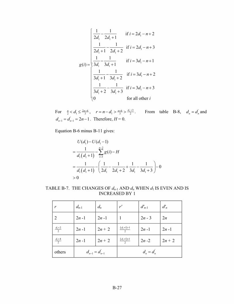
11 1

11 1

11 1

11 1

11 1

1 1 if 2 22 2 1

1 1 if 2 32 1 2 21 1 if 3 1

3 3 1( )1 1 if 3 2

3 1 3 21 1 if 3 3

3 2 3 30 for all other

i d nd d

i d nd d

i d nd dg i

i d nd d

i d nd d

i

⎧ − = − +⎪ +⎪⎪ − = − +⎪ + +⎪⎪

− = − +⎪ += ⎨

− = − ++ +

− = − ++ +

⎪⎪⎪⎪⎪⎪⎪⎩

For 2 6

12 3n nd −< ≤ , 1 36

1 3 2dnr n d ++= − > > . From table B-8, '

nd dn= and . Therefore, H = 0. '

1 1 2n nd d n− −= = −1 Equation B-6 minus B-11 gives:

( )

( )

1 12

31 1

1 1 1 1 1 1

( ) ( 1)1 ( )

1

1 1 1 1 1 01 2 2 2 3 3 3

0

n

i

U d U d

g i Hd d

d d d d d d

−

=

− −

= − −+

⎛ ⎞= − − + −⎜ ⎟+ + +⎝ ⎠>

∑

−

TABLE B-7. THE CHANGES OF dn-1 AND dn WHEN d1 IS EVEN AND IS

INCREASED BY 1

r dn-1 dn r′ d′n-1 d′n

2 2n -1 2n -1 1 2n - 3 2n

1 22

d + 2n -1 2n + 2 ( )1 1 12

d + − 2n -1 2n -1

1 42

d + 2n -1 2n + 2 ( )1 1 12

d + + 2n -2 2n + 2

others '1 1n nd d− −= '

n nd d=

B-27

TABLE B-8. THE CHANGES OF dn-1 AND dn WHEN IS ODD AND IS INCREASED BY 1

1d

r dn-1 dn r′ d′n-1 d′n

2 2n -2 2n -1 1 2n - 3 2n

1 12

d + 2n -1 2n + 2 ( )1 1 22

d + − 2n -1 2n -1

1 32

d + 2n -1 2n + 2 ( )1 12

d + 2n -1 2n -1

others '1 1n nd d− −= '

n nd d=

b. 2 6 2 3

13 3n d− −< ≤ n

n +

. Then

1

1 1

1

0 if 3 2 21 if 2 2 3 12 if 3 1 2

i

i d nk d n i d

d n i n

≤ < − +⎧⎪= − + ≤ < −⎨⎪ − + ≤ ≤ −⎩

1'

1

0 if 3 2 41 if 2 4 2i

i d nk

d n i n≤ < − +⎧

= ⎨ − + ≤ ≤ −⎩

• 2 3

1 3nd −= .

11 1

11 1

11 1

1 1 if 2 22 2 1

1 1 if 2 32 1 2 2( )1 1 if 3 1 2

3 3 10 for all other

i d nd d

i d nd dg i

i d n nd d

i

⎧ − = − +⎪ +⎪⎪ − = − +⎪ + += ⎨⎪⎪ − = − + = −

+⎪⎪⎩

1 33

3 2dnr ++= = , 1 2 1nd n− = − , 2 2nd n= + and

1

' ' 2n nd d n

−1= = − . Therefore,

( ) ( )( )32 1 1

2 1 2 1 2 2 2 1 2 2n n n n nH − − + − += − + = .

B-28

( )

( )

( ) ( )

( )

1 12

31 1

1 1 1 1 1 1

1 1 1 1

2 3 2 33 3

3 2

( ) ( 1)1 ( )

1

1 1 1 1 11 2 2 2 3 3 1

1 12 1 3 3 1

1 1 32 1 (2 3)(2 2) (2 1)(2 2)

1 7 9 32 2 (2 3)( 1) (2 1)( 1)

2 19 34 94 (2

n

i

n n

U d U d

g i Hd d

Hd d d d d d

Hd d d d

n n n n

nn n n n n

n n nn n

−

=

− −

− −

= − −+

⎛ ⎞= − − + − −⎜ ⎟+ + +⎝ ⎠

= − −+ +

= − −+ − − − +

⎛ ⎞−= ⋅ −⎜ ⎟− − − +⎝ ⎠

+ − +=

−

∑

3)( 1)(2 1)( 1)0

n n n− − +>

• 2 4

1 3nd −= . Then

11 1

11 1

11 1

11 1

1 1 if 2 22 2 1

1 1 if 2 32 1 2 2

( ) 1 1 if 3 1 33 3 1

1 1 if 3 2 23 1 3 20 for all other

i d nd d

i d nd d

g i i d n nd d

i d n nd d

i

⎧ − = − +⎪ +⎪⎪ − = − +⎪ + +⎪⎪= ⎨ − = − +⎪ +⎪⎪

= −

− = − + = −⎪ + +⎪⎪⎩

1 44

3 2dnr ++= = . Note that 2n-4 is an even number and is an integer. So, 1d

2 41 3

nd −= must also be even. Checking the corresponding entries in table B-7, ' 2 2n nd d n= = + ,

12

nd n

−1= − , and

1

' 2 2n

d n−

= − .

B-29

( ) ( ) ( )( )1 1 1 1 1

2 2 2 2 2 1 2 2 2 1 2 2n n n n n nH − + − + − −= + − + = .

( )

( )

( ) ( )

( )

1 12

31 1

1 1 1 1 1 1

1 1 1 1

2 4 2 43 3

( ) ( 1)1 ( )

1

1 1 1 1 11 2 2 2 3 3 2

1 22 1 3 3 2

1 2 12 1 (2 4)(2 2) (2 1)(2 2)

9 1 12(2 4)(2 1) (2 4)( 1) (2 1)( 2)

1 5 72 2( 2)(2 1)

n

i

n n

U d U d

g i Hd d

Hd d d d d d

Hd d d d

n n n n

n n n n n n

nn n

−

=

− −

− −

= − −+

⎛ ⎞= − − + − −⎜ ⎟+ + +⎝ ⎠

= − −+ +

= − −+ − − − −

= − −− − − − − −

−= ⋅

− −

∑

1( 1) (2 1)( 2)

1 32 2(2 1)( 2)0

n n n

n n

⎡ ⎤−⎢ ⎥− − −⎣ ⎦

= ⋅− −

>

• 2 5

1 3nd −= . Then

11 1

11 1

11 1

11 1

11 1

1 1 if 2 22 2 1

1 1 if 2 32 1 2 21 1 if 3 1 4

3 3 1( )1 1 if 3 2 3

3 1 3 21 1 if 3 3 2

3 2 3 30 for all oth

i d nd d

i d nd d

i d n nd dg i

i d n nd d

i d n nd d

− = − ++

− = − ++ +

− = − + =+=

−

− = − + = −+ +

− = − + = −+ +

er i

⎧⎪⎪⎪⎪⎪⎪⎪⎨⎪⎪⎪⎪⎪⎪⎪⎩

1 35

3 2dnr ++= > and 1( 1) 22

3 2' dnr + ++= = . Note that 2n-5 is an odd number and is an integer. So, 1d 2 5

1 3nd −= must also be odd. Checking the

corresponding entries of table B-8, and . Therefore,

' 2n nd d n= = + 21

1 1

' 2n n

d d n− −

= = − 0H = .

B-30

( )

( )

( )

1 12

31 1

1 1 1 1 1 1

1 1

( ) ( 1)1 ( )

1

1 1 1 1 1 01 2 2 2 3 3 3

16 10

n

i

U d U d

g i Hd d

d d d d d d

d d

−

=

− −

= − −+

⎛ ⎞= − − + −⎜ ⎟+ + +⎝ ⎠

=+

>

∑

−

c. 2 3

13 2n d n− < ≤ − .

1

1

0 if 3 2 21 if 2 2 2i

i d nk

d n i n≤ < − +⎧

= ⎨ − + ≤ ≤ −⎩

1'

1

0 if 3 2 41 if 2 4 2i

i d nk

d n i n≤ < − +⎧

= ⎨ − + ≤ ≤ −⎩

( )

⎪⎪⎪⎪

⎩

⎪⎪⎪⎪

⎨

⎧

+−=+−

+

+−=+−

=

i

ndidd

ndidd

ig

other allfor 0

32 if221

121

22 if121

21

111

111

Equation B-6 minus B-11 gives:

( )

( )

( )

1 12

31 1

1 1 1 1

1 1

( ) ( 1)1 ( )

1

1 1 11 2 2 2

12 1

n

i

U d U d

g i Hd d

Hd d d d

Hd d

−

=

− +

= − −+

⎛= − −⎜ ⎟+ +⎝ ⎠

= −+

∑

⎞−

(B-12)

Depending on d1, H takes on different values. There are four cases: • 2 2

1 3nd −= . Then 1 2

2dr += . Because 2n-2 is an even number and d1 is an

integer, 2 21 3

nd −= must be even. From table B-7, , ' '1 2 1

n nd d n−= = −

B-31

1 2nd n− = −1 , and 2 2nd n= + . Hence, 1 12 1 2 2n nH − −= − . Applying to

equation B-12 gives:

( )

( )( )( )

1 1

2 2 2 23 3

2

( ) ( 1)1 1

2 1 2 1 2

6 15 34 1 1 2 1 (2 1)0

n n

U d U d

n n

n nn n n n

− −

12

− +

⎛ ⎞= − −⎜ ⎟+ − −⎝ ⎠

+ −=

+ − − +

>

• 2 1

1 3nd −= . Then 1 1

2dr += . Because 2n-1 is an odd number and d1 is an

integer, 2 11 3

nd −= must be even. From table B-8, ,

, and

' '1 2 1

n nd d n−= = −

1 2nd n− = − 2 2 2nd n= + . Hence, ( )2 1 12 1 2 2 2 2n n nH − − += − + . Applying

to equation B-12 gives:

( )

( )( )( )

1 1

2 1 2 13 3

( ) ( 1)

1 2 1 12 1 2 1 2 2 2

5 14 2 1 1 10

n n

U d U d

n n nn

n n n

− − 2

− +

⎡ ⎤⎛ ⎞= − − +⎜ ⎟⎢ ⎥+ − − +⎝ ⎠⎣ ⎦−

=− + −

>

• 2

13 2n d n< < − . Then 'nd dn= and '

1n nd d 1− −= . So . 0H =

1 11 1

1( ) ( 1) 0 02 ( 1)

U d U dd d

− + = − >+

• . Then 1 2d n= − 2r = . From tables B-7 and B-8, ,

, and . Therefore, 1 2 1n nd d n−= = −

'1 2nd n− = − 3 n' 2nd = ( )1 1 2

2 3 2 2 1n n nH − −= + − . Applying to equation B-12 gives:

( )( )

( )( )( )

1 1

3 2

( ) ( 1)

1 1 12 2 2 1 2 3 2 2 1

2 5 8 62 2 1 2 1 (2 3)0

U d U d

n n n n n

n n nn n n n n

2

− +

⎡ ⎤⎛ ⎞= − +⎜ ⎟ −⎢ ⎥− − + − −⎝ ⎠⎣ ⎦

− + −=

− − − −

>

B-32

Claim 2: Given the number of tasks n and 12 d n 2≤ ≤ − , the Perfect Instance for n and d1 constructed above yields the minimum utilization of n tasks that perfectly utilize the processor among all those task sets that have the same and as the Perfect Instance. 1d 2d Proof: For n ≤ 9, the claim can be proved by enumeration. So, assume that n ≥ 10. Then d2 ≥ n ≥10. Let the perfect instance for d1 and n be . It will be proved by contradiction that TS has the minimum utilization among all task set instances that have the same and as TS. Suppose there is another task set

that perfectly utilizes the processor and

1 1 2 2{ (1, ), (1, ),..., (1, )}n nTS T d T d T d=

1d 2d' ' ' ' ' '

1 1 2 2' { (1, ), (1, ),..., (1, )}n nTS T d T d T d= '

1d d1= and

, but has a smaller utilization. Then there must be some task T'2d d= 2

j

2

j, 3 ≤ j ≤ n, such that . Let T'

jd d< i be such a task that has the minimum deadline. It will be shown that , , and i case by case. {3,..., 2}i n∉ − 1i n≠ − n≠

1. . {3,..., 2}i n∉ −

Proof. Suppose on the contrary, there is an i, 3 i n≤ ≤ − , such that . Using time demand analysis, it can be proved that:

i idd >′

1 2 21 2 2 'i i n i… d dd d d+ d= = = = + < =′ ′ ′ .

2

1

1 1 1 11

1 1 1( )1

n n n

j i j i j ij j i j

n

j ii i n

n iU Ud d dd

n id d j i d

= = =

−

= −

− +′ − ≥ − = −+′

− +> − + +

+ + −

∑ ∑ ∑

∑ 1

nd

There are two cases: • . 2i n= −

Then,

2 2 1

3 1 1 11 (

n n nd d dU U− − −+′ − = − + + )

nd . By construction of , id

− Either . 1 2 2n n nd d d− −= ≥ +

2 2 2 2

3 1 1 1( )1 2n n n n

U Ud d d d− − − −

′ − > − + + >+ + +

02

− Or and . 1 2 1n nd d− −≥ + 1 3n nd d −≥ +

2 2 2 2

3 1 1 1( )1 1n n n n

U Ud d d d− − − −

′ − > − + + >+ + +

04

B-33

• For all other i ,

1 1 1 1 01 1

n n

j i j ii j i i

n i n iU Ud d d d j i= =

− + − +′ − = − > − >+ + +∑ ∑ −

.

2. . 1i n≠ −

Proof. Suppose on the contrary 1i n= − . By construction, either 1nd − 1t= or . It will be proved that under both cases, 1 1 1nd t− = + 0U U′ − > , where U and U are

the total utilization of TS′ and TS, respectively. ′

• . 1 1nd t− =

For 2 ≤ j ≤ n - 2, dj < t1 < 2d2 ≤ 2d′j. So T′j makes exactly two requests before time . The total number of requests from T′1t 1, T′2… T′, n-1 before is 1t

1

12( 3) 1t

dR n⎡ ⎤= + − +⎢ ⎥ . By equation B-2, 1R t= . None of T′1, T′2 ,…, T′i-1, T′i+1, …,

T′n-2 will make their third requests at time t1. Because , T1 1 1t'n nd d− −> = 1'n− will not make a request at time t1. Thus, the first request of T′n will be executed. This means that . 1 1 21 2n n nd dd d − −= = + ≤′ ′ For , by assumption, 3 2j n≤ ≤ − j jdd ≤′ .

1 1 1 1

1 1 1 1 2 1 1( ) ( )' ' 1n n n n n n

U Ud d d d d d d− − − −

′ − ≥ + − + = − ++ n

1t

'

By tables B-3 and B-4, one can find that for each pair of and such that

, the right-hand side of the above inequality is positive, i.e., . 1nd − nd

1nd − = 0U U′ − >

• . 1 1 1n nd d t− = = +

It will be shown that in this case it is impossible that . By tables B-3 and B-4, , where 2

1 1n ndd − −>′

1 22 2 2 jt d d= − < 2j n≤ ≤ − . So at time t1, task makes exactly two requests. By equation B-2, all requests from T′

' jT1, …, T′n-1 will be

executed before , and no request is released at t1t 1 by task , where , because

' jT2 j n≤ ≤ − 2 1 2 ' jt d< . It has been proved that t1 is not a multiple of

. Thus, will not make a request at t1'd d= 1 1'T 1. If 1 1'n nd d− −> , will not make the second request at t

1'nT −

1. In order to be a task set perfectly utilizing the processor, the first request of T′n must be executed at t1. Therefore,

, which is a contradiction to the assumption that . 1 1' nnd d − −= =′ nd 1 1'n nd d− −>

B-34

3. . i n≠ Suppose , i.e., is the only task such that i n= nT 'id d i< . There are two cases to consider depending on the relationship between and . nd 2d • . 22nd d≤

By assumption, and 2'd d= 2 2' jd d≤ for 3j ≥ . So 2 'n jd d≤ for 2j ≥ . On the other hand, . So, for all ' j jd d d< < n 2 1j n≤ ≤ − , task makes exactly two requests before time

' jT1nt d= − , and it will not make the third request before time

. It has been shown that all those requests by nd 1, 2 1,..., nT T T −′ ′ ′ can be executed before time , and will not make a request at 1nd − 1'T 1nd − . So the first request of will be executed at time nT ′ 1nd − . However, this means that , which contradicts the assumption that

n ndd =′'n nd d< .

• . 22 2nd d= +

It is known that . To prove the claim, there are two cases to consider, depending on whether or

3 2' 'd d d≥ = 2

2 23'd d> 3'd d= . If , then 3 2dd >′ 3T ′ will not make its third request before 22nd d 2= + . So, using the same argument for the case , it can be shown that 22nd ≤ d n ndd =′ , which contradicts the assumption that dn < d′n. Consider now the case 3 2dd =′ . The proof is quite involved. The idea is to show that the task set TS can be obtained from TS by a series of modifications of and for . Each step can be described as follows: Starting from i = 3, if

, then decrease d

′ id

nd 3i ≥

i idd <′ i to id ′ and if necessary, increase to make the modified task set to continue perfectly utilizing the processor. Let the modified

be , the new task set be , and be the total utilization of . Let S denote the maximum index i such that

nd

nd ( )nd i iTS iU iTS'id id< . By assumption, . After

S steps, the instance 1S n≤ −

TS ′ is obtained. Let U denote the total utilization of the perfect instance. In the following, it will be proved that U , which is a contradiction. For convenience let

U ′<2U U= and 2(2) 2 2nd d= + .

The proof is by induction on i - the index of the task besides that is changed at each step.

nT

B-35

Induction hypotheses: There are three hypotheses:

1. For 3 1 , either i S≤ ≤ − ( ) ( 1) 1n nd i d i= − + , or ;( ) ( 1) 2n nd i d i= − + 2 ' ( 1) 2i nd d i di< − ≤ .

2. For 3 1 , i S≤ ≤ − 2( ) 3nd i d≤ , and

1 12 2

1 1

2 2 (2 2( ) 2 21 1n

i r d i d rd i d i d id d

)⎡ ⎤ ⎡+ − − − −= + + = + +

⎤⎢ ⎥ ⎢− − ⎥⎢ ⎥ ⎢ ⎥

(B-13)

3. for iU U< 3 i S≤ ≤ .

Base case: . 3i = 1. or (3) (2) 1n nd d= + (3) (2) 2n nd d= + ; 3 32 ' (2) 2nd d d< ≤ .

By assumption, 3 2 22 ' 2 (2) 2 2 2nd d d d 3d= < = + ≤ . To prove the remainders, there are two cases depending on r.

a. . 1 1r d= − Then . The number of requests of before time

is 2 . When is changed to , which is equal to , the number of requests by in the new task instance before

time is 3, i.e., one more than that of in the original instance. In order to make the new instance perfectly utilize the processor, needs to be increased by at least 1. However, because

3 2 2d d= + 3T

2(2) 2 2n nd d d= = + 3d 3'd

2d 3'T 3TS

nd 3T

nd

22nd d 2= + is a multiple of , at time , will make another request. Therefore, needs to be

increased by at least 2. In fact, needs to be increased by exactly 2. Because the period of any other task has not been changed, 4 ≤ j ≤ n - 1, . So, it makes exactly two requests before time

, which is the same as in the original task set. The requests of task T

1d nd 1T nd

nd

jT

22 2 2j nd d d> + = 4+

2nd +

2 before 2d2 + 4 is still the same -- 3. Therefore, . (3)n nd d=

b. . 1 1r d< −

Then . The number of requests of before is 2 . When is changed to , which is equal to

, the number of requests by in the new task instance before

3 2 1d d= + 3T

2(2) 2 2n nd d d= = + 3d 3'd

2d 3'T 3TS nd

B-36

is 1 more than that of in the original instance. In order to make the new instance perfectly utilizes the processor, needs to be increased by at least 1. It is enough that is increased by exactly 1. Because

is not a multiple of , will not make any request at time . The period of any other tasks ,

3T

nd

nd

22 2d d= +n 1d 1T

nd jT 4 1j n≤ ≤ − , is not changed. So makes exactly two requests before time ' jT 2nd + , which is the same as

in the original task set. Therefore, 2(3) 1 2 3n nd d d= + = + . 2. and 2(3) 3nd d≤ 1 1

1 1

3 2 2 3 (2 2r− )2 21 1(3) 2 3 2 3r d d

n d dd d d+ − − −− −

⎡ ⎤ ⎡ ⎤= + + = + +⎢ ⎥ ⎢ ⎥ .

It has already been shown that if 1 1r d= − , then ; otherwise,

2(3) 2 4nd d= +

2(3) 2 3nd d= + . It is obvious that . In both cases, can be written in the following way:

2(3) 3nd ≤ d(3)nd

1 12 2

1 1

3 2 2 3 (2 2 )(3) 2 3 2 31 1n

r d d rd d dd d

⎡ ⎤ ⎡+ − − − −= + + = + +

⎤⎢ ⎥ ⎢− − ⎥⎢ ⎥ ⎢ ⎥

3. . 3U U<

Since only the deadlines of and are modified, the difference between the total utilization of the new instance and that of the original instance

is

3T nT

3UU

33 3 2 3

1 1 1 1 1 1 1 1( ) ((3) (3) 2 2n n n

U Ud d d d d d d d

− = + − + = + − ++2

) .

It has been shown that either 3 2 2d d= + and , or

and 2(3) 2 4nd d= +

3 2 1d d= + 2(3) 2 3nd d= + . It is easy to show that in both cases, . Therefore, 3 0U U− > 3U U< .

Induction step: Suppose the hypotheses are true for 3, 4, …, i-2, where i ≤ S. Now there is the task set 1iTS − . One needs to change to d′id i, and change

to if necessary. The hypotheses need to be proved to be true for i . ( 1)nd i − ( )nd i

First, it will be proved that 2 ( 1)i nd d i< − . Suppose . It will be shown that there is a contradiction to the assumption that TS has a smaller utilization than the perfect instance. When is decreased to d′

2 ( 1)i nd d i≥ −′

id i, the number of requests of T′i before time ( 1)nd i − has not changed, i.e., it makes two requests.

B-37

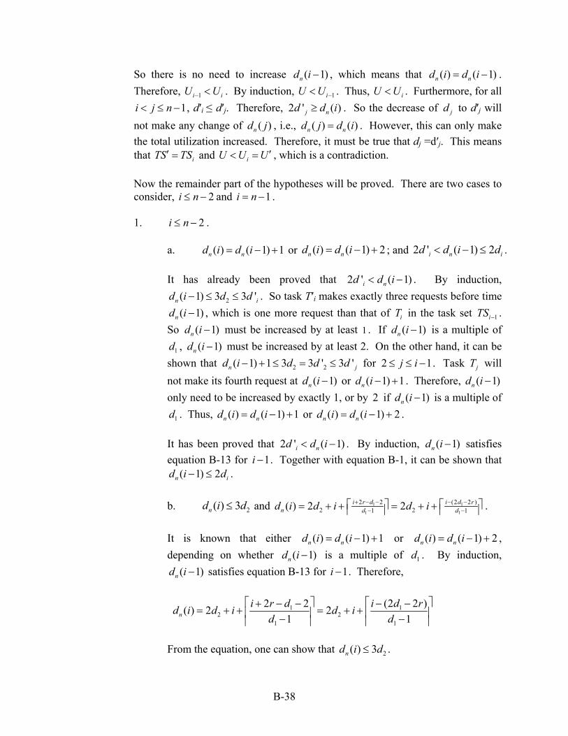
So there is no need to increase ( 1)nd i − , which means that . Therefore, . By induction,

( ) ( 1)n nd i d i= −

1iU U− < i 1iU U −< . Thus, iU U< . Furthermore, for all , d′1i j n< ≤ − i ≤ d′j. Therefore, . So the decrease of to d′2 ' ( )j nd d i≥ jd j will

not make any change of , i.e., ( )nd j ( ) ( )n nd j d i= . However, this can only make the total utilization increased. Therefore, it must be true that dj =d′j. This means that and iTS TS′ = iU U U ′< = , which is a contradiction. Now the remainder part of the hypotheses will be proved. There are two cases to consider, and 2i n≤ − 1i n= − . 1. . 2i n≤ −

a. or ( ) ( 1) 1n nd i d i= − + ( ) ( 1) 2n nd i d i= − + ; and . 2 ' ( 1) 2i nd d i d< − ≤ i

It has already been proved that 2 ' ( 1)i nd d i< − . By induction,

. So task T′2( 1) 3 3 'nd i d d− ≤ ≤ i i makes exactly three requests before time , which is one more request than that of in the task set ( 1)nd i − iT 1iTS − .

So must be increased by at least 1 . If is a multiple of , must be increased by at least 2. On the other hand, it can be

shown that

( 1)nd i − ( 1)nd i −

1d ( 1)nd i −

2 2( 1) 1 3 3 ' 3 'n jd i d d d− + ≤ = ≤ for 2 1j i≤ ≤ − . Task will not make its fourth request at

jT( 1)nd i − or ( 1) 1nd i − + . Therefore, ( 1)nd i −

only need to be increased by exactly 1, or by if is a multiple of . Thus,

2 ( 1)nd i −

1d ( ) ( 1) 1n nd i d i= − + or ( ) ( 1) 2n nd i d i= − + . It has been proved that 2 ' ( 1)i nd d i< − . By induction, satisfies equation B-13 for

( 1)nd i −1i − . Together with equation B-1, it can be shown that

. ( 1) 2n id i d− ≤ b. and 2( ) 3nd i d≤ 1 1

1 1

2 2 (2 2 )2 21 1( ) 2 2i r d i d r

n d dd i d i d i+ − − − −− −

⎡ ⎤ ⎡= + + = + + ⎤⎢ ⎥ ⎢ ⎥ .

It is known that either ( ) ( 1) 1n nd i d i= − + or , depending on whether

( ) ( 1) 2n nd i d i= − +( 1)nd i − is a multiple of . By induction,

satisfies equation B-13 for 1d

( 1)nd i − 1i − . Therefore,

1 12 2

1 1

2 2 (2 2( ) 2 21 1n

i r d i d rd i d i d id d

)⎡ ⎤ ⎡+ − − − −= + + = + +

⎤⎢ ⎥ ⎢− − ⎥⎢ ⎥ ⎢ ⎥

From the equation, one can show that 2( ) 3nd i d≤ .

B-38

c. . iU U< It has already been proved that 2 ' ( 1) 2i nd d i di< − < . So

and . It has already been proved that . Therefore,

' ( ( 1) 1) 2i nd d i≤ − − / ( 1) 2i nd d i≥ − /( ) ( 1) 2n nd i d i≤ − +

11 1 1 1( ) ( )

( ) ( 1)2 1 2( ) (

( 1) 1 ( 1) 2 ( 1) ( 1)3 ( 1) 3 3

( ( 1) 1)( ( 1) 2) ( 1)6

( 1) ( ( 1) 1)( ( 1) 2)0

i ii n i n

n n n n

n

n n n

n n n

U Ud d i d d i

d i d i d i d id i

d i d i d i

d i d i d i

− − = + − +−

> + − +1 )

− − − + − −− +

= −− − − + −

=− ⋅ − − − +

≥

2. . 1i n= −

It is known that 1S n≤ − and i ≤ S. So i = S. What remains to be proved for this case is 1nU U −< .

Like the previous case, it can be proved that 1 12 ' ( 2) 2n n nd d n d− −< − ≤ . To prove the remaining hypotheses, there are two cases to consider:

a. . 2( 2) 3nd n d− < If is changed to 1nd − 1'nd − , the number of requests by T′n-1 increases by 1 before time ( 2)nd n − . ( 2)nd n − must be increased by at least 1. If

is a multiple of , then ( 2)nd n − +1 1d ( 2)nd n − needs to be increased by at least 2. It will be shown that one needs to increase by exactly 1 or 2.

It is necessary to ensure that other tasks T′j, 2 2j n≤ ≤ − , does not make an extra request after ( 2)nd n − is increased by 1 or 2. If

, then 2( 2) 3nd n d− ≤ − 2 2( 2) 2 3nd n d− + ≤ and T′j will not make its fourth request before . Thus, 23d 2( 1) 3nd n d− ≤ . As before, it can be shown that 2nU U 1n− −< by simple calculation. Therefore, 1nU U −< . Otherwise, 2( 2) 3nd n d 1− = − . In this case, will not make a request at

time , since 1T

23d −1 1 12

d r+ ≤ (which is implied by the assumption that and table B-3). Similarly, T′22nd d= + 2 j will not make its fourth request

before . Thus, 23d 2( 1) 3nd n d− = and one can show that . 1nU U −<

B-39

b. . 2( 2) 3nd n d− = In this case, if dn-1 is changed to d′n-1, it is not true that one only needs to increase ( 2)nd n − by 1 or 2 as before, because after is increased by 1 or , T′

( 2)nd n −2 2, and T′3 will make their fourth requests. It may happen that

while these requests are being executed, T′4, …also make requests during this period. So there is no chance to execute the first request of T′n before finishing other requests with higher priority. In order to prove the hypotheses, one cannot do the simple calculation this time. One needs to compare U and 1nU − term by term. d′i can be estimated based on the induction.

1

1

1

1

1

1

1 (2 2 )2 1

1 (2 2 )1

2

(2 2 )1

2

( 1) 1'2

2 ( 1) 1

2

2

2

2

2

ni

i d rd

i d rd

i d rd

d id

d i

id

id

− − −−

− − −−

− −−

− −⎡ ⎤≤ ⎢ ⎥⎢ ⎥⎡ ⎤⎡ ⎤+ − + −⎢ ⎥⎢ ⎥=⎢ ⎥⎢ ⎥

⎡ ⎤⎡ ⎤− + ⎢ ⎥⎢ ⎥≤ +⎢ ⎥⎢ ⎥

⎡ ⎤− + ⎢ ⎥≤ +

1

2 21 1

12

1

1

1

3 22 21 1

( 1)21

( 3) 11

ii r i r dd d i d id d

i d rd id

n i dd

( 1)⎡ ⎤ ⎡+ − + − − −= + − + = + − +

⎤⎢ ⎥ ⎢− − ⎥⎢ ⎥ ⎢⎡ ⎤− − +

= + − + ⎢ ⎥−⎢ ⎥+ − −

≤−

⎥

1 1

1 1

( 1) (2 2 ) (11 1

i d r i d r i d rd d d

⎡ ⎤ ⎡ ⎤ ⎡− − + − − − − +− ≤ ≤⎢ ⎥ ⎢ ⎥ ⎢− −⎢ ⎥ ⎢ ⎥ ⎢

1

1

1)1

⎤⎥− ⎥

1

1

1

1

( 1)1

( 1)1

1

1

2'

22

2(2 3) 3

2( 1)

i d rd

i i

i d rd

i

id d

id

n i d rd

− − +−

− − +−

⎡ ⎤− + ⎢ ⎥≤ −

− +≤ −

+ − − −≤

−

B-40

( 1)111

1 1

1

1 1

1 1

22

( 2)( 1) ( 1)2( 1)

( 3) 1 (2 3) 31 2( 1)

11

1 1

11

1 1

1

'1 1' '

'

( 3) 3( 1)[( 3) 1][(2 3) 3]

( 3)( 1)[( 3) ][(2 3) ]

1

i d rd

i i

i i i i

i

i i

i d i d rd

n i d n i d rd d

d dd d d d

d d

i d rdn i d n i d r

i ddn i d n i d

d

− − +−− +

− − + − + −−

+ − − + − − −− −

−− =

≥

≥

− + +≥ −

+ − − + − − −−

≥ −+ − + −

−≥

1

3( 3)(2 3)

id n i n i

−⋅

+ − + −

11 3

2

3 1 1

2

3 2 2 2

222

23 2 2

2

23 2 2 2

2

3

1 1 1 1( ) ( )' '

1 1 1 1 1( ) ( ) (0 )' '

1 1 2 1 1( ) ( ) (0 )' 3 2 2 2 2

21 1( )' 3 ( 1)

1 1 1 1( )' 3 ( 1)

i n n

ni ii i i i

n

i i i n n n

n

i i i

n

i i i

n

i i i

n

i

U Ud d d d

d d d d d

d d d d d

dd d d d

d d d d d

=

−= =

−

= − −

−

=

−

=

−

=

−

=

− = − = −

> − + − + −

> − + − + −− +

+= − −

−

> − − +−

>

∑ ∑

∑

∑

∑

∑

∑ 22 2

21 1

23 1 12

1 12

3 1 1

21

231

1 1 1 1( )' 3 ( 1)

1 11 1( ) ( )' 3[( 1) ] [( 1) ]( 1)

1 11 1( ) [ ]' (3 6) ( 2)( 1)

1 3 1 1[( ) ( )]( 3)(2 3) (3 6) ( 2)( 1)

0 when

i in

i i in

i i i

n

i

d d d d nd d

d d n d r n d r nd d

d d n d n n dd i

d n i n i n n n

−

=

−

=

−

=

− − +−

− −> − − +

− − − − −

− −> − − +

− − −

− −> − +

+ − + − − − −>

∑

∑

∑10n ≥

It has just been proved that SU U< . Note that STS TS ′= , so U U ′< .

B-41

B.5.2 PERFECT INSTANCE WHEN d1 AND d2 ARE ARBITRARY.

In the following, an instance of n tasks for given d1 and d2 will be constructed. For convenience, the constructed instance will be called the perfect instance for n, d1, and d2. It will first be shown that the instance perfectly utilizes the processor. It is then proved that the instance constructed for d1 = n - 1 has the minimum total utilization among all task instances that have n tasks and perfectly utilize the processor. Construction of Perfect Instances. Given the number of tasks n, T1(1, d1) and T2(1, d2), where d1 ≤ n-1, d2 ≤ n and d1≤ d2, construct T3(1, d3), . . . , Tn(1, dn) as follows: 1. For 3 ≤ i ≤ n - 2, let di be the maximum integer such that

1 2

1 2

( 6)

( 6) for

i id di d d

t tid d

d n i

t n i t

⎧ ⎡ ⎤ ⎡ ⎤= + + + −⎪ ⎢ ⎥ ⎢ ⎥⎨

⎡ ⎤ ⎡ ⎤⎪ ≤ + + + − ≤⎢ ⎥ ⎢ ⎥⎩d

(B-14)

2. In order to define dn-1 and dn, define the first two variables t1 and t2

• Let t1 be the maximum integer such that

1 1

1 2

1 2

1

1

(2 7)

(2 7) for

t td d

t td d

t n

t n

⎧ ⎡ ⎤ ⎡ ⎤= + + −⎪ ⎢ ⎥ ⎢ ⎥⎨

⎡ ⎤ ⎡ ⎤⎪ ≤ + + − ≤⎢ ⎥ ⎢ ⎥⎩t t

(B-15)

• Let t2 be the minimum integer such that

2 2

1 2

1 2

2

2

(2 5)

(2 5) for

t td d

t td d

t n

t n

⎧ ⎡ ⎤ ⎡ ⎤= + + −⎪ ⎢ ⎥ ⎢ ⎥⎨

⎡ ⎤ ⎡ ⎤⎪ < + + − <⎢ ⎥ ⎢ ⎥⎩t t

(B-16)

If t2 = kd3 + 1 for some k, then dn = t2 + 1 and dn-1 = t1. Otherwise, t2 ≠ kd3 + 1 for any k. If t2 = t1 +2, let dn-1 = dn = t1 +1 = t2 –1; else t2 ≥ t1 +3, let dn-1 = t1 and dn = t2. It will first be proved that the constructed perfect instance has several properties. It will then be proved that this instance perfectly utilizes the processor.

Claim 3: For 3 ≤ i ≤ n - 1, di is neither a multiple of d1 nor a multiple of d2. Proof. Consider first the case 3 ≤ i ≤ n-2. Let di = ki1d1 +r i1 = ki2d2 + ri2, where ki1and ki2 are integers, 0 ≤ ri1 ≤ d1 – 1 and 0 ≤ ri2 ≤ d2 - 1. It will be proved that both ri1 and ri2 are greater than 0; if not, then there are two cases to consider.

B-42

a. Either ri1 = 0 or ri2= 0. Suppose that ri1= 0, then 1 1

1 1i id dd d+⎡ ⎤ ⎡ ⎤= +⎢ ⎥ ⎢ ⎥ and

2 2

1i id dd d+⎡ ⎤ ⎡ ⎤=⎢ ⎥ ⎢ ⎥ .

Therefore, equation B-14 also holds for i when t = di + 1. But by definition, di is the largest integer that satisfies equation B-14. This is a contradiction. The same conclusion can be reached for the case ri2= 0.

b. ri1 = ri2= 0, because 2 ≤ d1 ≤ d2, 1 1

2 1i id dd d+⎡ ⎤ ⎡ ⎤= +⎢ ⎥ ⎢ ⎥ and

2 2

2 1i id dd d+⎡ ⎤ ⎡ ⎤= +⎢ ⎥ ⎢ ⎥ . Therefore,

equation B-14, also holds when t = di + 2, again, a contradiction.

If i = n - 1, by the construction, either dn-1 = t1 or dn-1 = t1 + 1. In the former case, t1 cannot be a multiple of d1, because otherwise the same contradiction can be obtained as before. In the latter case, dn-1 = t1 +1, which means that t2 = t1 +2. By equations B-15 and B-16,

1 1 1

1 2 1

2 2t t td d d d+ +⎡ ⎤ ⎡ ⎤ ⎡ ⎤ ⎡ ⎤+ = +⎢ ⎥ ⎢ ⎥ ⎢ ⎥ ⎢ ⎥

1

2

t . However, this equation holds only when t1 + 1 is not a multiple of d1

or d2. Therefore, in both cases, dn-1 is not a multiple of d1 or d2. Claim 4: di +1 = di + x for 3 ≤ i ≤ n – 3, where x = 1 or 2 or 3. Proof. Let di = ki1 d1 + ri1 = ki2d2 + ri2, where 1 ≤ ri1 ≤ d1 –1 and 1 ≤ ri2 ≤ d2 -1. Similarly, let di+1 = k(i+1)1 d1 + r(i+1)1= k(i+1)2 d2 + r(i+1)2 ,where 1 ≤ r(i+1)1 ≤ d1 - 1 and 1 ≤ r(i+1)2 ≤ d2 – 1. There are three cases to consider: • ri1 ≤ d1 – 2 and ri2 ≤ d2 - 2.

Then

1 1

1 1i id dd d+⎡ ⎤ ⎡ ⎤= +⎢ ⎥ ⎢ ⎥ and

2

1idd d+⎡ ⎤ ⎡ ⎤=⎢ ⎥ ⎢ ⎥2

id . Let t = di + 1. It is easy to show that equation B-

14 holds for i + 1, but for any t′ > t, equation B-14 does not hold. Therefore, di+1 = di + 1.

• ri1= d1 - 1 and ri2

≤ d2 – 3, or ri1 ≤ d1 - 3 and ri2

= d2 - 1.

Suppose that ri1 = d1-1 and ri2

≤ d2-3, then 1 1

2 1i id dd d+⎡ ⎤ ⎡ ⎤= +⎢ ⎥ ⎢ ⎥ and

2

2idd d+

2

id⎡ ⎤ ⎡ ⎤=⎢ ⎥ ⎢ ⎥ . Let t = di +

2. One can show that equation B-14 holds for i + 1, but for any t′ > t , equation B-14 does not hold. Therefore, di+1 = di + 2 in this case. For the case ri1

≤ d1 - 3 and ri2 = d2 -

1, the proof is the same.

• ri1= d1 - 1 and ri2

≤ d2 – 2, or ri1 ≤ d1 - 2 and ri2

= d2 - 1.

Using the same argument as above, one can prove that di+1 = di + 3.

Claim 5: Let d3 = k1d1 + r1 = k2d2 + r2, where 1 ≤ r1 ≤ d1 - 1 and 1 ≤ r2 ≤ d2 - 1. Express t1 in terms of d3. The expression depends on the value of r1 and r2, and it is shown in tables B-9 to B-16.

B-43

• r1 = r2 = 1. See table B-9.

TABLE B-9. VALUE OF t1 WHEN r1 = r2 = 1

d2 = 3 d2 = 4 d2 = 5 or 6 or 7 d2 ≥ 8 d1 = 2 2d3 – 15 2d3 – 11 2d3 – 9 2d3 – 7 d1 = 3 2d3 – 9 2d3 – 7 2d3 – 6 2d3 – 6 d1 ≥ 4 - 2d3 – 7 2d3 – 5 2d3 – 5

• r1 = 1 and r2 = 2. See table B-10.

TABLE B-10. VALUE OF t1 WHEN r1 = 1 AND r2 = 2

d2 = 3 d2 = 4 d2 ≥ 5 d1 = 2 2d3 – 11 2d3 – 9 2d3 – 7 d1 = 3 2d3 – 6 2d3 – 6 2d3 – 6 d1 ≥ 4 2d3 – 5 2d3 – 5

• r1 = 1 and 22

23 dr ≤≤ . See table B-11.

TABLE B-11. VALUE OF t1 WHEN r1 = 1 AND 2223 dr ≤≤

d1 = 2 and r2 = 1 d1 = 2 and r2 ≥ 4 d1≥3 2d3 – 7 2d3 – 5 2d3 – 4

• r1 = 1 and 22

2dr > . If d2 = 5 and r2 = 3, then t1 = 2d3 –7; otherwise, see table B-12.

TABLE B-12. VALUE OF t1 WHEN r1 = 1 AND 222dr >

r2 = 2 1

2d + or 2 2

2d + or 2 3

2d + r2 = 2 4

2d + r2 ≥ 2 5

2d +

d1 = 2 2d3 – 5 2d3 – 5 2d3 – 3 d1≥ 3 2d3 – 4 2d3 – 3 2d3 – 3

• 21

12 dr ≤≤ and r2 = 1. If r1 = 2, then t1 = 2d3– 5; otherwise, t1 = 2d3 - 4.

• 2112 dr ≤≤ and 22

22 dr ≤≤ .

If r1 = r2 = 2, then t1 = 2d3 – 5; otherwise t1 = 2d3 - 3.

B-44

• 2112 dr ≤≤ and 22

2dr > , or 211dr > and 22

22 dr ≤≤ . See tables B-13 and B-14, respectively.

TABLE B-13. VALUE OF t WHEN1 21

12 dr ≤≤ AND 222dr >

r2 = 2 12

d + r2 = 2 22

d + r2 ≥ 2 32

d +

2d3 – 3 2d3– 3 2d3 – 2

TABLE B-14. VALUE OF t1 WHEN 211dr > AND 22

22 dr ≤≤

r1 = 1 12

d + r1 = 1 22

d + r1 ≥ 1 32

d +

2d3 – 3 2d3– 3 2d3 – 2

• 211dr > and r2 = 1. See table B-15.

TABLE B-15. VALUE OF t1 WHEN 21

1dr > AND r2 = 1

r1 = 1 12

d + and d1 = 3 r1 = 1 12

d + and d3 > 3 r1 = 1 22

d + or 1 32

d + r1 ≥ 1 42

d +

2d3 – 5 2d3 – 4 2d3– 4 2d3 – 3 • 21

1dr > and 222dr > . See table B-16.


1dr > AND 222dr >

r2 = 2 12

d + r2 = 2 22

d + r2 ≥ 2 32

d +

r1 = 1 12

d + 2d3 – 3 2d3– 3 2d3 – 2

r1 = 1 22

d + 2d3– 3 2d3– 3 2d3 – 1

r1 ≥ 1 32

d + 2d3– 2 2d3 – 1 2d3 – 1

To check the correctness of the values of t1 for different cases, it is sufficient to show that in each case

1 1

1 2

1 11 1 (t t

d dt n− −⎡ ⎤ ⎡ ⎤− ≤ + + −⎢ ⎥ ⎢ ⎥ 2 7)

B-45

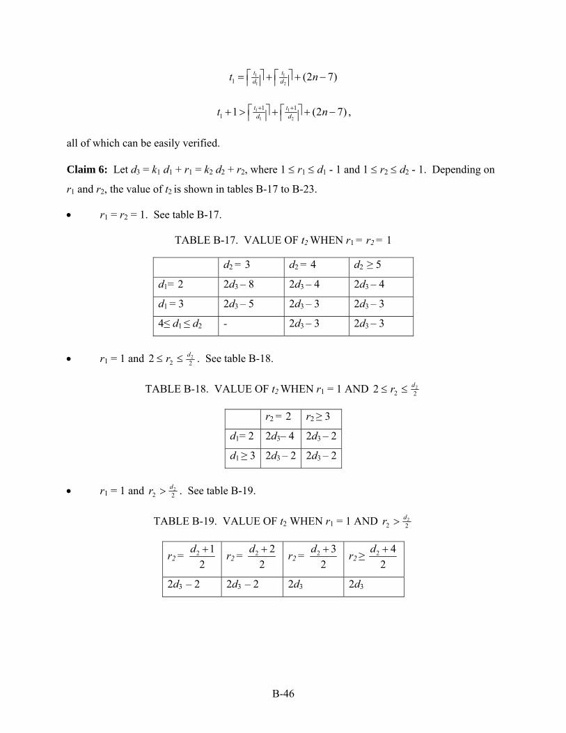
1 1

1 21 (2 7)t td dt n⎡ ⎤ ⎡ ⎤= + + −⎢ ⎥ ⎢ ⎥

1 1

1 2

1 11 1 (t t

d dt n+ +⎡ ⎤ ⎡ ⎤+ > + + −⎢ ⎥ ⎢ ⎥ 2 7) ,

all of which can be easily verified. Claim 6: Let d3 = k1 d1 + r1 = k2 d2 + r2, where 1 ≤ r1 ≤ d1 - 1 and 1 ≤ r2 ≤ d2 - 1. Depending on

r1 and r2, the value of t2 is shown in tables B-17 to B-23.

• r1 = r2 = 1. See table B-17.

TABLE B-17. VALUE OF t2 WHEN r1 = r2 = 1

d2 = 3 d2 = 4 d2 ≥ 5

d1= 2 2d3 – 8 2d3 – 4 2d3 – 4

d1 = 3 2d3 – 5 2d3 – 3 2d3 – 3

4≤ d1 ≤ d2 - 2d3 – 3 2d3 – 3

• r1 = 1 and 22

22 dr ≤≤ . See table B-18.

TABLE B-18. VALUE OF t2 WHEN r1 = 1 AND 2222 dr ≤≤

r2 = 2 r2 ≥ 3

d1= 2 2d3– 4 2d3 – 2

d1 ≥ 3 2d3 – 2 2d3 – 2

• r1 = 1 and 22

2dr > . See table B-19.

TABLE B-19. VALUE OF t2 WHEN r1 = 1 AND 222dr >

r2 = 2 12

d + r2 = 2 22

d + r2 = 2 32

d + r2 ≥ 2 42

d +

2d3 – 2 2d3 – 2 2d3 2d3

B-46

• 2112 dr ≤≤ and r2 = 1.

t2 = 2d3- 2.

• 2112 dr ≤≤ and 22

22 dr ≤≤ .

t2 = 2d3 – 1.

• 2112 dr ≤≤ and 22

2dr > , or 211dr > and 22


TABLE B-20. VALUE OF t2 WHEN 2112 dr ≤≤ AND 22

2dr >

r2 = 2 12

d + r2 = 2 22

d + r2 ≥ 2 32

d +

2d3 – 1 2d3 2d3


1dr > AND 2222 dr ≤≤

r1 = 1 12

d + r1 = 1 22

d + r1 ≥ 1 32

d +

2d3 – 1 2d3 2d3

• 21

1dr > and r2 = 1. See table B-22.

TABLE B-22. VALUE OF t2 WHEN 211dr > AND r2 = 1

r1 = 1 12

d + or 1 22

d + r1 = 1 32

d + r1 ≥ 1 42

d +

2d3 – 2 2d3 2d3

• 21


B-47

TABLE B-23. VALUE OF t2 WHEN 211dr > AND 22

2dr >

r2 = 2 12

d + r2 = 2 22

d + R2 ≥ 2 32

d +

r1 = 1 12

d + 2d3 – 1 2d3 + 1 2d3+ 1

r1 = 1 22

d + 2d3 + 1 2d3 +1 2d3 + 1

r1 ≥ 1 32

d + 2d3+ 1 2d3+ 1 2d3 + 1

Claim 7: Based on t1 and t2, dn-1 and dn are constructed as shown in tables B-24 to B-26.

• r1 = r2 = 1. See table B-24.

TABLE B-24. VALUE OF dn-1 AND dn WHEN r1 = r2 = 1

d2 = 3 d2 = 4 d2 = 5 or 6 d2 ≥ 7

d1 =2 dn-1 = 2d3 – 15

dn = 2d3 – 8

dn-1 = 2d3 – 11

dn = 2d3 – 4

dn-1 = 2d3 – 9

dn = 2d3 – 4

dn-1 = 2d3 – 7

dn = 2d3 – 4

d1 = 3 dn-1 = 2d3 – 9

dn = 2d3 – 5

dn-1 = 2d3 – 7

dn = 2d3 – 3

dn-1 = 2d3 – 6

dn = 2d3 – 3

dn-1 = 2d3 – 6

dn = 2d3 – 3

4 ≤ d1≤ d2 -

-

dn-1 = 2d3 – 7

dn = 2d3 – 3

dn-1 = 2d3 – 4

dn = 2d3 – 4

dn-1 = 2d3 – 4

dn = 2d3 – 4

• r1 = 1 and r2 = 2. See table B-25.

TABLE B-25. VALUE OF dn-1 AND dn WHEN r1 = 1 AND r2 = 2

d2 = 3 d2 = 4 d2 ≥ 5

d1 =2 dn-1 = 2d3 – 11

dn = 2d3 – 4

dn-1 = 2d3 – 9

dn = 2d3– 4

dn-1 = 2d3 – 7

dn = 2d3– 4

d1 = 3 dn-1 = 2d3 – 6

dn = 2d3 – 2

dn-1 = 2d3 – 6

dn = 2d3 – 2

dn-1 = 2d3 – 6

dn = 2d3 – 2

d1 ≥ 4 dn-1 = 2d3 – 5

dn = 2d3 – 2

dn-1 = 2d3 – 5

dn = 2d3 – 2

B-48

• r1 = 1 and 2223 dr ≤≤ . See table B-26.

TABLE B-26. VALUE OF dn-1 AND dn WHEN r1 = 1 AND 2223 dr ≤≤

d1 = 2 and r2 = 3 d1 = 2 and r2 ≥ 4 d2 ≥ 3

dn-1 = 2d3 – 7

dn = 2d3 – 2

dn-1 = 2d3 – 5

dn = 2d3 – 2

dn-1 = 2d3 – 3

dn = 2d3 – 3

• r1 = 1 and 22

23 dr ≤≤ .

If d2 = 5 and r2 = 3, then dn-1 = 2d3-7 and dn = 2d3-2; otherwise, see table B-27.

TABLE B-27. VALUE OF dn-1 AND dn WHEN r1 = 1 AND 2223 dr ≤≤

r2 = 2 12

d + or 2 22

d + r2 = 2 32

d + r2 = 2 42

d + r2 ≥ 2 52

d +

d1 = 2 dn-1 = 2d3 – 5

dn = 2d3 – 2

dn-1 = 2d3 – 5

dn = 2d3

dn-1 = 2d3 – 5

dn = 2d3

dn-1 = 2d3 – 3

dn = 2d3

d1 ≥ 3 dn-1 = 2d3 – 3

dn = 2d3 – 3

dn-1 = 2d3 – 4

dn = 2d3

dn-1 = 2d3 – 3

dn = 2d3

dn-1 = 2d3 – 3

dn = 2d3

• 21

12 dr ≤≤ and r2 = 1.

If r1 = 2, then dn-1= t1= 2d3-5 and dn = t2 = 2d3 – 2; otherwise, dn-1 = dn = 2d3 - 3.

• 2112 dr ≤≤ and 22

22 dr ≤≤ .

If r1 = r2 = 2, then dn-1 = 2d3 - 5 and dn = 2d3 –1; otherwise, t2 = t1 + 2 and hence

dn-1 = dn = t1 + 1 = 2d3 - 2.

• 2112 dr ≤≤ and 22

2dr > , or 211dr > and 22


TABLE B-28. VALUE OF dn-1 AND dn WHEN 2112 dr ≤≤ AND 22

2dr >

r2 = 2 12

d + r2 = 2 22

d + r2 ≥ 2 32

d +

dn-1 = 2d3 – 2 dn = 2d3 – 2

dn-1 = 2d3 – 3 dn = 2d3

dn-1 = 2d3 – 1 dn = 2d3 – 1

B-49

TABLE B-29. VALUE OF dn-1 AND dn WHEN 211dr > AND 22

22 dr ≤≤

r1 = 1 12

d + r1 = 1 22

d + r1 ≥ 1 32

d +

dn-1 = 2d3– 2 dn = 2d3 – 2

dn-1 = 2d3 – 3 dn = 2d3

dn-1 = 2d3 – 1 dn = 2d3 – 1

• 211dr > and r2 = 1. See table B-30.

TABLE B-30. VALUE OF dn-1 AND dn WHEN 211dr > AND r2 = 1

r1 = 1 12

d + and d1=3 r1 = 1 12

d + and d1 >3 r1 = 1 22

d + r1= 1 32

d + r1 ≥ 1 42

d +

dn-1 = 2d3 – 5

dn = 2d3

dn-1 = 2d3 – 3

dn = 2d3 – 3

dn-1 = 2d3 – 3

dn = 2d3

dn-1 = 2d3 – 4

dn = 2d3

dn-1 = 2d3 – 3

dn = 2d3

• 21


TABLE B-31. VALUE OF dn-1 AND dn WHEN 211dr > AND 22

2dr >

r2 = 2 1

2d + r2 = 2 2

2d + r2 ≥ 2 3

2d +

r1= 1 12

d + dn-1 = 2d3 – 2

dn = 2d3 – 2

dn-1 = 2d3 – 3

dn = 2d3 + 2

dn-1 = 2d3 – 2

dn = 2d3 + 2

r1= 1 22

d + dn-1 = 2d3 – 3

dn = 2d3 + 2

dn-1 = 2d3 – 3

dn = 2d3 + 2

dn-1 = 2d3 – 1

dn = 2d3 + 2

r1 ≥ 1 32

d + dn-1 = 2d3 – 2

dn = 2d3 + 2

dn-1 = 2d3 – 1

dn = 2d3 + 2

dn-1 = 2d3 – 1

dn = 2d3 + 2

Claim 8: dn - 1 is not a multiple of d1 nor d2.

Proof. There are three cases to consider:

• dn - 1 = t2, i.e., dn = t2 + 1.

By construction of dn, this case happens when t2 = kd3 + 1 for some k. From the tables in claim 7, one can see that this case happens only when 21

1dr > and 222dr > , where t2 = 2d3

+ 1. Let d3 = k1d1 + r1. Then t2 = 2k1d1+2r1+1. Since 11121 −≤≤ drd ,

B-50

1111 212121 ddrd <−≤+≤+ . Therefore, (2k1 + 1)d1 < t2 < (2k1 + 2)d1, which implies that t2 cannot be a multiple of d1. Similarly, one can prove that t2 is not a multiple of d2.

• dn - 1 = t2 - 1, i.e., dn = t2.

Suppose that t2 - 1 is a multiple of d1 but not d2, then 2 2

1 1

1 1t td d−⎡ ⎤ ⎡ ⎤= −⎢ ⎥ ⎢ ⎥ and 2 2

2 2

1 1t td d−⎡ ⎤ ⎡ ⎤= −⎢ ⎥ ⎢ ⎥ .

Hence, equation B-16 also holds for t2 - 1. However, by definition, t2 is the minimum integer that satisfies equation B-16. This is a contradiction. Using a similar argument, one can prove that dn - 1 cannot be a multiple of d2.

• dn - 1 = t2 - 2, i.e., dn = t2 - 1.

In this case, dn = dn-1, which means that t2 = t1 + 2. By equation B-15 and B-16, one must have 2 2

1

2td d−⎡ ⎤ ⎡=⎢ ⎥ ⎢ 1

t ⎤⎥ and 2

2

2td d−⎡ ⎤ ⎡=⎢ ⎥ ⎢

2

2

t ⎤⎥ . Thus, dn - 1 or t2 - 2 cannot be a multiple of d1 or d2.

Theorem 12: The perfect instance T1, T2, . . . , Tn constructed above perfectly utilizes the processor. Below are some lemmas about the DM schedule for the perfect instance. The theorem follows directly from these lemmas and the definition of perfect utilization. Lemma 2: For the DM schedule of the perfect instance, there is no idle time before t1. Proof. It is enough to prove that at any time t < t1, the number of requests R from T1, . . . , Tn-2, Tn-1 is greater than or equal to t. There are two cases depending on t.

• t = di. t ≤ dj for j ≥ i. So Ti, …, Tn-1 each makes exactly one request before t. On the other hand, dk ≤ t ≤ 2dk for 3 ≤ k ≤ i –1. So T3, . . ., Ti-1 each makes exactly two requests. Therefore, the total number of requests before time t from T1, . . . , Tn-1 is

1 26t t

d dR n i⎡ ⎤ ⎡ ⎤= + + + −⎢ ⎥ ⎢ ⎥ . By construction, t =di = R.

• di < t < di+1. • t < dj for j ≥ i+1. So Ti+1, … ,Tn-1 each makes exactly one request before t. On the other

hand, dj < t ≤ 2dj for 3 ≤ j ≤ i. So T3, . . ., Ti each makes exactly two requests. Therefore, at time t, the total number of requests from T1, . . . , Tn-1 is

1 2( 1) 6t t

d dR n i⎡ ⎤ ⎡ ⎤= + + + + −⎢ ⎥ ⎢ ⎥ . By the construction of di+1, t ≤ R.

Lemma 3: There is no suspending request from T3, . . . , Tn-2, Tn-1 at t1.

B-51

Proof. One can show that the number of requests from T1, . . . ,Tn-1 during the period [0, t1) is equal to t1. Lemma 4: None of T4, . . ., Tn-2 will make a request during the period [t1, dn-1]. Proof. Because for 4 ≤ j ≤ n-2, T1 31 2 1 2j nd t d d d< < − ≤ + < j

3

j makes exactly two requests before t1 and will not make its third request before dn-1. Lemma 5: There is no idle time during the period [t1, dn-1) and there is no request from T1, T2, T3, and Tn-1 at dn-1. Therefore, the first request from Tn will be executed at dn-1. Proof. Let t1 ≤ t ≤ dn-1. To prove that there is no idle time from t1 to dn-1, it is sufficient to show that at t the number of requests from all tasks except Tn is greater than or equal to t.

Consider first . At the requests from T2 2nd t d= ≤ t 1 and T2 are

1

td⎡ ⎤⎢ ⎥ and

2

td⎡ ⎤⎢ ⎥ , respectively.

Task Tj, 2 ≤ j ≤ n-1, has two requests. Together with T3, … , Tn-1, there are 2n-6 requests. The total number of requests by T1, . . . , Tn-1 is

1 2(2 6)t t

d dR ⎡ ⎤ ⎡ ⎤ n= + + −⎢ ⎥ ⎢ ⎥ . By the definition of t2,

1 2(2 5)t t

d dt n⎡ ⎤ ⎡ ⎤< + + − ≤⎢ ⎥ ⎢ ⎥ R .

If dn = t2 -1 or dn = t2 + 1, one can use a similar argument. It will now be shown that there is no request released at dn-1. It has already been shown that dn-1 is not a multiple of d1 or d2, so neither T1 nor T2 makes a request at dn-1. Since either d3 < dn-1 < 2d3 or , T31 2 1nd d− = + 1 will not make its third or fourth request at dn-1. By construction, either dn-1 = dn-1 – 1 or dn-1 < dn-1 < 2dn-1. So Tn-1 will not make its second or third request at time dn-1. Combining Lemmas 2, 3, and 4, the processor is busy from time 0 to dn-1, all requests from T1, …, Tn-1 have been executed before time dn-1, and there is no request released at time dn-1. So the first request of Tn will be executed at time dn-1. By definition, the perfect instance perfectly utilizes the processor. Thus, theorem 12 is proved. B.5.3 PERFECT INSTANCE WHEN 1

2 1 2nd d +≥ > .

First, the following lemma is very easy to verify. Lemma 6: Given n and 1

2 1 2nd d +≥ > , let the perfect instance for , dn 1, and d2 be

, then d1 1 2 2 3 3{ (1 ) (1 ) (1 ) ..., (1 )}n nTS T d T d T d T d= , , , , , , , 3 = n + 1. Claim 9: Given n and 1

2 1 2nd d +≥ > , let the perfect instance for , dn 1, and d2 be

, and the total utilization be U(d1 1 2 2 3 3{ (1 ) (1 ) (1 ) ..., (1 )}n nTS T d T d T d T d= , , , , , , , 2). Let

B-52

1 2 3 3

' ' ' '1 2 2{ (1 ) (1 1) (1 ) ..., (1 )}

n nTS T d T d d T d T d′ = , , , = + , , , , '

) be the perfect instance for , dn 1, and

, and its total utilization be 2 1d + 2( 1U d + , then U(d2) ≥ U(d2+1).

The proof is by showing that '1 1

2 21

( ) ( 1) 0i i

n

d di

U d U d=

− + = − >∑ for every possible d1 and d2. The

cases are listed in table B-32.

TABLE B-32. THE CASES OF di AND d′i DEPENDING ON d1 AND d2

d2 d1

2 2 42 3[ ,n n+ − ] 2 3

3n− 2 2

3n− 2 1

3n− 2

3n 2 1

3n+ 2 2

3n+ 2 3

3[ , 3n n+ − ] n-2 n-1

2 2 42 3[ ,n n+ − ] 7 8 9 10 11 11 11 12 12 15

2 33

n− * 16 ** ** 17 ** ** 12 12 15 2 2

3n− * * 18 ** ** 17 ** 12 12 19

2 13n− * * * 20 ** ** 21 13 14 19

23n * * * * 20 ** ** 13 22 19

2 13n+ * * * * * 20 ** 13 23 19

2 23

n+ * * * * * * 20 24 23 19 2 3

3[ , 3n n+ − ] * * * * * * * 25 23 19 n-2 * * * * * * * * 26 19 n-1 * * * * * * * * * 27

Note: * impossible cases because d1 ≤ d2. ** impossible cases because both d1 and d2 are integers. Other entries are the numbers of lemmas that prove the corresponding cases. From lLemma 6, it follows that d3 = d′3 = n+1, 1 11r n d= + − , 2 1r n d2= + − and r′2 = r2-1. Let

'

2 1 11 3

(ii

ndi d

S −

== ∑ )− and ' ' 11

1 1 1 12 ( ) (

n nn nd dd d

S++

= + − + ) . Then 2 2

12 2 1( 1)( ) ( 1) d dU d U d S S⋅ + 2− + = − − .

The values of di, 4 ≤ i ≤ n, depend on the values of d1 and d2. Since and depend on the values of d

1S 2Si, their values depend on d1 and d2 as well. The claim will be proved for each case.

For all cases, the idea is the same: From d1 and d2, one can obtain , r1r 2 and r′2. Applying claim 7, it is easy to calculate S2. To calculate S1, one needs to find di and d′i for 4 ≤ i ≤ n-2. Specifically, one needs to express di and d′i in terms of . As it has been shown in claim 4, d3d i+1 is usually greater than di by 1. Thus, di = d3+i-3. But it has been proved that cannot be a multiple of d

id1 or d2. Therefore, one needs to do some corrections to this formula to jump over

those multiples of d1 or d2. Initially, di is increased by 1 to get di+1, so di = d3 + i-3. At some point di = 2d1 –1. To jump over 2d1, the formula becomes di = d3+i-2. After that di is continuously increased by 1 to di+1, until at another point where di = 2d2-1 or di = 3d1-1, then the formula is changed again. These points (the indices of the tasks i, 3 ≤ i ≤ n-2) where the formula is corrected varies with d1 and d2.

B-53

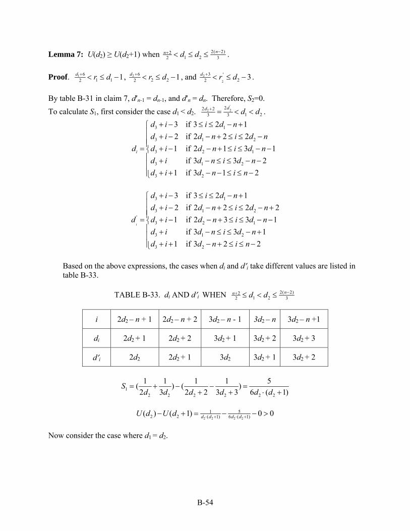
Lemma 7: U(d2) ≥ U(d2+1) when 2( 2)21 22 3

nn d d −+ < ≤ ≤ . Proof. 1 6

1 12 1d r d+ < ≤ − , 2 62 22 1d r d+ < ≤ − , and 2

2

3 '22 3d r d+ < ≤ − .

By table B-31 in claim 7, d′n-1 = dn-1, and d′n = dn. Therefore, S2=0.

To calculate S1, first consider the case d1 < d2. '

2 222 21 23 3

dd d d+ = < < .

3 1

3 1 2

3 2 1

3 1 2

3 2

3 if 3 2 1 2 if 2 2 2 1 if 2 1 3 1

if 3 3 2 1 if 3 1 2

i

d i i d nd i d n i d n

d d i d n i d nd i d n i d nd i d n i n

+ − ≤ ≤ − +⎧⎪ + − − + ≤ ≤ −⎪⎪= + − − + ≤ ≤ − −⎨⎪ + − ≤ ≤ − −⎪

+ + − − ≤ ≤ −⎪⎩

3 1

3 1 2'

3 2 1

3 1 2

3 2

3 if 3 2 12 if 2 2 2 21 if 2 3 3 1

if 3 3 11 if 3 2 2

i


d d i d n i d nd i d n i d nd i d n i n

+ − ≤ ≤ − +⎧⎪ + − − + ≤ ≤ − +⎪⎪= + − − + ≤ ≤ − −⎨⎪ + − ≤ ≤ − +⎪

+ + − + ≤ ≤ −⎪⎩

Based on the above expressions, the cases when di and d′i take different values are listed in table B-33.

TABLE B-33. di AND d′i WHEN 2( 2)2

1 22 3nn d d −+ ≤ < ≤

i 2d2 – n + 1 2d2 – n + 2 3d2 – n - 1 3d2 – n 3d2 – n +1

di 2d2 + 1 2d2 + 2 3d2 + 1 3d2 + 2 3d2 + 3

d′i 2d2 2d2 + 1 3d2 3d2 + 1 3d2 + 2

12 2 2 2 2 2

1 1 1 1 5( ) ( )2 3 2 2 3 3 6 (

Sd d d d d d

= + − − =1)+ + ⋅ +

2 2 2 2

512 2 ( 1) 6 ( 1)( ) ( 1) 0 0d d d dU d U d ⋅ + ⋅ +− + = − − >

Now consider the case where d1 = d2.

B-54

3 1

3 1 1

3 1

3 if 3 2 11 if 2 2 3 11 if 3 2

i

d i i d nd d i d n i d n

d i d n i n

+ − ≤ ≤ − +⎧⎪= + − − + ≤ ≤ − −⎨⎪ + + − ≤ ≤ −⎩

3 1

3 1'

3 1 1

3 1 1

3 1

3 if 3 2 12 if 2 21 if 2 3 3 1

if 3 or 3 11 if 3 2 2

i

d i i d nd i i d n

d d i d n i d nd i i d n d nd i d n i n

+ − ≤ ≤ − +⎧⎪ + − = − +⎪⎪= + − − + ≤ ≤ − −⎨⎪ + = − − +⎪

+ + − + ≤ ≤ −⎪⎩


TABLE B-34. di AND d′i WHEN 2( 2)21 22 3

nn d d −+ ≤ = ≤

i 2d2 – n + 2 3d2 – n 3d2 – n +1

di 2d2 + 2 3d2 + 2 3d2 + 3

d′i 2d2+1 3d2 + 1 3d2 + 2

11 1 1 1

1 1 1 1( ) (2 1 3 1 2 2 3 3

Sd d d d

= + − − )+ + + +

2 22 2 1 1 1 1

1 1 1 1 1( ) ( 1) (( ) ( )) 0 0( 1) 2 1 3 1 2 2 3 3

U d U dd d d d d d

− + = − + − − − >+ + + + +

.

Lemma 8: U(d2) ≥ U(d2+1) when 2 2

12 3n nd 4+ −≤ ≤ and 2 3

2 3nd −= .

Proof. 1 6

1 2dr +≥ , 2 56

2 3 2dnr ++= = , ' 2

2 2 31 nd d= + = , and 2

2

2' 33 2

dnr ++= = . By table B-31 in claim 7, d′n = dn and d′n-1 = dn-1 = 2d3 + 2 = 2(n+2). Therefore, S2 = 0.

3 1

3 1 2

3 2 1

3 1 2

3

3 if 3 2 12 if 2 2 21 if 2 1 3 1

if 3 1 3 21 if 4 or 3 or 2

i


d d i d n i d nd i d n i d nd i i n n n

+ − ≤ ≤ − +⎧⎪ + − − + ≤ ≤ −⎪⎪= + − − + ≤ ≤ − −⎨⎪ + − − ≤ ≤ −⎪

+ + = − − −⎪⎩

−

B-55

3 1

3 1 2'

3 2 1

3 1

3 if 3 2 12 if 2 2 2 21 if 2 3 3 1

if 3 2

i


dd i d n i d nd i d n i n

+ − ≤ ≤ − +⎧⎪ + − − + ≤ ≤ + −⎪= ⎨ + − − + ≤ ≤ − −⎪⎪ + − ≤ ≤ −⎩


TABLE B-35. di AND d′i WHEN 2 21 22 3

n nd d 3+ −≤ = ≤

i 2d2 – n + 1 2d2 – n + 2 n -4 n -3 n -2

di 2d2 + 1 2d2 + 2 2n-2 2n-1 2n

d′i 2d2 2d2+1 2n-3 2n-2 2n-1

12 2

1 1 1 1( ) (2 2 3 2 2 2

Sd n d n

= + − +− +

)

2 2 2 2

1 1 1 1 12 2 ( 1) 2 2 3 2 2 2( ) ( 1) ( ) ( ) 0 0d d d n d nU d U d ⋅ + − +− + = − + − + − > .

Lemma 9: U(d2) ≥ U(d2+1) when 2 2

12 3n nd 4+ −≤ ≤ and 2 2

2 3nd −= .

Proof. 1 61 2

dr +≥ , 2 452 3 2

dnr ++= = , 2

' 2 12 31 nd d += + = , and

'2

2

1' 23 2

dnr ++= = . By table B-31 in claim 7, dn-1 = 2d3-1 = 2n+1, dn = 2d3+2 = 2n+4, d′n-1 = 2d3 –2 = 2n, and d′n = 2d3 + 2 = 2n + 4. Therefore,

21

2 (2 1)S

n n=

+

3 1

3 1 2

3 2 1

3 1 2

3

3 if 3 2 12 if 2 2 21 if 2 1 3 1

if 3 3 2 41 if 3 or 2

i


d d i d n i d nd i d n i d n nd i i n n

+ − ≤ ≤ − +⎧⎪ + − − + ≤ ≤ −⎪⎪= + − − + ≤ ≤ − −⎨⎪ + − ≤ ≤ − − =⎪

+ + = − −⎪⎩

−

B-56

3 1

3 1 2'

3 2 1

3 1

3 if 3 2 12 if 2 2 2 21 if 2 3 3 1

if 3 2

i



+ − ≤ ≤ − +⎧⎪ + − − + ≤ ≤ − +⎪= ⎨ + − − + ≤ ≤ − −⎪⎪ + − ≤ ≤ −⎩



n nd d 2+ −≤ = ≤

i 2d2 – n + 1 2d2 – n + 2 n -4 n -3

di 2d2 + 1 2d2 + 2 2n-1 2n

d′i 2d2 2d2+1 2n-2 2n-1

12 2

1 12 ( 1) 2 ( 1)

Sd d n n

= ++ −

2 2 2 2

1 1 1 12 2 ( 1) 2 ( 1) (2 1) 2 (2 1)( ) ( 1) ( ) 0d d d d n n n nU d U d ⋅ + + − +− + = − + − > .

Lemma 10: U(d2) ≥ U(d2+1) when 2 2

12 3n nd 4+ −≤ ≤ and 2 1

2 3nd −= .

Proof. 1 6

1 2dr +≥ , 2 34

2 3 2dnr ++= = ,

2

' 2 22 31 nd d += + = , and 21

2 3dnr +2= = . By tables B-29 and B-31 in

claim 7, dn-1 = 2d3-1 = 2n+1, dn = 2d3+2 = 2n+4, and d′n-1 = d′n = 2d3 -1 = 2n+1. Therefore,

23

(2 1)(2 4)S

n n=

+ +

3 1

3 1 2

3 2 1

3 1 2

3

3 if 3 2 12 if 2 2 21 if 2 1 3 1

if 3 3 2 31 if 2

i


d d i d n i d nd i d n i d n nd i i n

+ − ≤ ≤ − +⎧⎪ + − − + ≤ ≤ −⎪⎪= + − − + ≤ ≤ − −⎨⎪ + − ≤ ≤ − − =⎪

+ + = −⎪⎩

−

3 1

3 1 2'

3 2 1

3 1

3 if 3 2 12 if 2 2 2 21 if 2 3 3 1

if 3 2

i



+ − ≤ ≤ − +⎧⎪ + − − + ≤ ≤ − +⎪= ⎨ + − − + ≤ ≤ − −⎪⎪ + − ≤ ≤ −⎩

B-57



n nd d 1+ −≤ = ≤

i 2d2 – n + 1 2d2 – n + 2 n -3

di 2d2 + 1 2d2 + 2 2n

d′i 2d2 2d2+1 2n-1

12 2

1 12 ( 1) 2 (2 1)

Sd d n n

= ++ −

2 2 2 2

31 1 12 2 ( 1) 2 ( 1) 2 (2 1) (2 1)(2 4)( ) ( 1) 0d d d d n n n nU d U d ⋅ + + − + +− + = − − − > .

Lemma 11: U(d2) ≥ U(d2+1) when 2 2

12 3n nd 4+ −≤ ≤ and 2

2 3nd = or 2 1

3n+ or 2 2

3n+ .

Proof. First, calculate S1.

3 1

3 1 2

3 2 1

3 1

3 if 3 2 12 if 2 2 21 if 2 1 3 1

if 3 2

i



+ − ≤ ≤ − +⎧⎪ + − − + ≤ ≤ −⎪= ⎨ + − − + ≤ ≤ − −⎪⎪ + − ≤ ≤ −⎩

3 1

3 1 2'

3 2 1

3 1

3 if 3 2 12 if 2 2 2 21 if 2 3 3 1

if 3 2

i



+ − ≤ ≤ − +⎧⎪ + − − + ≤ ≤ − +⎪= ⎨ + − − + ≤ ≤ − −⎪⎪ + − ≤ ≤ −⎩


TABLE B-38. di AND d′i WHEN 2 2

12 3n nd 4+ −≤ ≤ AND 2

2 3nd = OR 2 1

3n+ OR 2 2

3n+

i 2d2 – n + 1 2d2 – n + 2

di 2d2 + 1 2d2 + 2

d′i 2d2 2d2+1

B-58

12 2

12 ( 1)

Sd d

=+

To calculate S2, consider the following three cases: 1. 2

2 3nd = .

1 6

1 2dr +≥ , 2 23

2 3 2dnr ++= = ,

2

' 2 32 31 nd d += + = , and

'2

2

1'3 2

dnr −= = . By tables B-29 and B-31 in claim 7, dn-1 = 2d3-1 = 2n+1, dn = 2d3+2 = 2n+4, and d′n-1 = d′n=2d3 -1 =2n+1. Therefore,

23

(2 1)(2 4)S

n n=

+ +

2 2 2 2

31 12 2 ( 1) 2 ( 1) (2 1)(2 4)( ) ( 1) 0d d d d n nU d U d ⋅ + + + +− + = − − > .

2. 2

2 3nd = .

1 6

1 2dr +≥ , 2 12

2 3 2dnr ++= = ,

2

' 2 42 31 nd d += + = , and

'2

2

2' 13 2

dnr −−= = . By tables B-29 and B-31 in claim 7, dn-1= 2d3-2 = 2n, dn = 2d3+2 = 2n+4, and d′n-1 = d′n= 2d3 -1 = 2n+1. Therefore,

22 1

2 1 2 4 2S

n n= − −

+ +1n

2 2 2 2

1 1 2 1 12 2 ( 1) 2 ( 1) 2 1 2 4 2( ) ( 1) ( ) 0d d d d n n nU d U d ⋅ + + + +− + = − − − − > .

3. 2

2 3nd = .

1 6

1 2dr +≥ , 21

2 3 2dnr += = ,

2

' 2 52 31 nd d += + = , and 2

2

3' 23 2

dnr −−= = . By table B-29 in claim 7, dn-1 = dn = 2d3 -1 = 2n + 1 and d′n-1 = d′n = 2d3 -1 = 2n+1. Therefore, S2 = 0.

2 2 2 2

1 12 2 ( 1) 2 ( 1)( ) ( 1) 0 0d d d dU d U d ⋅ + +− + = − − > .

Lemma 12: U(d2) ≥ U(d2+1) when 2 2

12 3n nd 2+ −≤ ≤ and 2 3

23 3n d n+ ≤ ≤ − . Proof. 1 42

1 3 2dnr ++≥ ≥ , 2

2 3 24 dnr≤ ≤ < , and 2

2

'2 23 1 dr r≤ = − < . By table B-29 in claim 7, dn = d′n

and dn-1 = d′n-1. Therefore, S2 = 0.

B-59

1. 22 21 3

dd −≤ .

3 1

3 1 1

3 1 2

3 2

3 if 3 2 12 if 2 2 31 if 3 1 2 1

if 2 2

i



+ − ≤ ≤ − +⎧⎪ + − − + ≤ ≤ −⎪= ⎨ + − − + ≤ ≤ − −⎪⎪ + − ≤ ≤ −⎩

3 1

3 1 1'

3 1 2

3 2

3 if 3 2 12 if 2 2 31 if 3 1 2 1

if 2 2 2

i



+ − ≤ ≤ − +⎧⎪ + − − + ≤ ≤ −⎪= ⎨ + − − + ≤ ≤ − +⎪⎪ + − + ≤ ≤ −⎩

If i = 2d2-n, then di = n + 1 + 2d2 – n = 2d2 – n = 2d2 + 1 and d′i = di –1 = 2d2. If i = 2d2 - n + 1, then di = n + 1 + 2d2 - n + 1 = 2d2+ 2 and d′i = di – 1 = 2d2+1.

12 2 2 2

1 1 12 2 2 2 ( 1

Sd d d d

= − =)+ ⋅ +

2 22 2 2 2

1 1( ) ( 1) 0 0( 1) 2 ( 1)

U d U dd d d d

− + = − − >⋅ + ⋅ +

.

2. 22 1

1 3dd −= .

3 1

3 1 1 2

3 2

3 if 3 2 12 if 2 2 3 2 1

if 2 2i

d i i d nd d i d n i d n d n

d i d n i n

+ − ≤ ≤ − +⎧⎪= + − − + ≤ ≤ − = − −⎨⎪ + − ≤ ≤ −⎩

3 1

3 1 1 2'

3 2 2

3 2

3 if 3 2 12 if 2 2 3 2 11 if 2 or 2 1

if 2 2 2

i

d i i d nd i d n i d n d n

dd i i d n d nd i d n i n

+ − ≤ ≤ − +⎧⎪ + − − + ≤ ≤ − = − −⎪= ⎨ + − = − − +⎪⎪ + − + ≤ ≤ −⎩

If i = 2d2 - n, then di = n + 1 + 2d2 - n = 2d2+ 1 and d′i = di – 1 = 2d2. If i = 2d2 - n + 1, then di = n + 1 + 2d2 - n + 1 = 2d2+ 2 and d′i = di – 1 = 2d2+1.

12 2

12 ( 1)

Sd d

=+

B-60

2 22 2 2 2

1 1( ) ( 1) 0 0( 1) 2 ( 1)

U d U dd d d d

− + = − − >⋅ + ⋅ +

.

3. 22

1 3dd = .

212if222if123if

23

2

21

1

3

3

3

−≤≤+−−≤≤+−

+−≤≤

⎪⎩

⎪⎨

⎧

+−+−+

=nind

ndindndi

ididid

di

3 1

3 1 1'

3 2

3 2

3 if 3 2 12 if 2 2 3 21 if 2 1

if 2 2 2

i

d i i d nd i d n i d n d n

dd i i d nd i d n i n

+ − ≤ ≤ − +⎧⎪ + − − + ≤ ≤ − = −⎪= ⎨ + − = − +⎪⎪ + − + ≤ ≤ −⎩

2

If i = 2d2 - n + 1, then di = n + 1 + 2d2 - n + 1 = 2d2 + 2 and d′i = di – 1 = 2d2 + 1.

12 2

12(2 1)( 1)

Sd d

=+ +

2 22 2 2 2

1 1( ) ( 1) 0 0( 1) 2(2 1) ( 1)

U d U dd d d d

− + = − − >⋅ + + ⋅ +

.

4. 22 1

1 3dd += .

3 1

3 1

3 2

3 if 3 2 12 if 2 2 2

if 2 1 2i

d i i d nd d i d n i d

d i d n i n

+ − ≤ ≤ − +⎧⎪= + − − + ≤ ≤ −⎨⎪ + − + ≤ ≤⎩

2 n−

3 1

'3 1 2

3 2

3 if 3 2 12 if 2 2 2 1

if 2 2 2i


d i d n i n

+ − ≤ ≤ − +⎧⎪= + − − + ≤ ≤ − +⎨⎪ + − + ≤ ≤ −⎩

.

If i = 2d2 - n + 1, then di = n + 1 + 2d2 - n + 1 = 2d2 + 2 and d′i = di – 2= 2d2.

12 2

12 ( 1)

Sd d

=+

2 22 2 2 2

1 1( ) ( 1) 0 0( 1) 2 ( 1)

U d U dd d d d

− + = − − >⋅ + ⋅ +

.

B-61

5. 22 21 3

dd += .

3 1

3 1

3 2

3 2

3 if 3 2 12 if 2 2 21 if 2 1

if 2 2 2

i


dd i i d nd i d n i n

+ − ≤ ≤ − +⎧⎪ + − − + ≤ ≤ −⎪= ⎨ + − = − +⎪⎪ + − + ≤ ≤⎩

2

−

If , 2 2d n= −

3 1'

3 1 2

3 if 3 2 12 if 2 2 2 2 2i

d i i d nd

d i d n i d n n+ − ≤ ≤ − +⎧

= ⎨ + − − + ≤ ≤ − + = −⎩

Otherwise,

3 1

'3 1 2

3 2

3 if 3 2 12 if 2 2 2 2

if 2 3 2i


d i d n i n

+ − ≤ ≤ − +⎧⎪= + − − + ≤ ≤ − +⎨⎪ + − + ≤ ≤ −⎩

.

If i = 2d2 - n + 1, then di = n + 1 + 2d2 - n + 1 –1 = 2d2 + 1 and d′i = di – 1 = 2d2. If i = 2d2 - n + 2, then di = n + 1 + 2d2 - n + 2 = 2d2 + 3 and d′i = di – 2 = 2d2 +1.

12 2 2 2

1 1 32 2 3 2 (2

Sd d d d

= − =3)+ +

2 22 2 2 2

1 1( ) ( 1) 0 0( 1) 2 ( 1)

U d U dd d d d

− + = − − >⋅ + ⋅ +

.

6. 22 3

1 3dd += .

3 1

3 1 2

3 2 2

3 2

3 if 3 2 12 if 2 2 21 if 2 1 or 2 2

if 2 3 2

i


dd i i d n d nd i d n i n

+ − ≤ ≤ − +⎧⎪ + − − + ≤ ≤ −⎪= ⎨ + − = − + − +⎪⎪ + − + ≤ ≤ −⎩

3 1

'3 1 2

3 2

3 if 3 2 12 if 2 2 2 2

if 2 3 2i


d i d n i n

+ − ≤ ≤ − +⎧⎪= + − − + ≤ ≤ − +⎨⎪ + − + ≤ ≤ −⎩

B-62

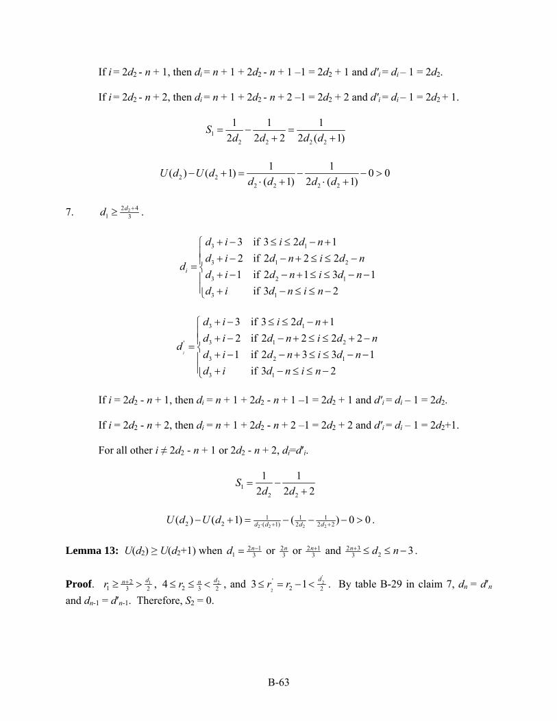
If i = 2d2 - n + 1, then di = n + 1 + 2d2 - n + 1 –1 = 2d2 + 1 and d′i = di – 1 = 2d2. If i = 2d2 - n + 2, then di = n + 1 + 2d2 - n + 2 –1 = 2d2 + 2 and d′i = di – 1 = 2d2 + 1.

12 2 2 2

1 1 12 2 2 2 (

Sd d d d

= − =1)+ +

2 22 2 2 2

1 1( ) ( 1) 0 0( 1) 2 ( 1)

U d U dd d d d

− + = − − >⋅ + ⋅ +

7. 22 4

1 3dd +≥ .

3 1

3 1 2

3 2 1

3 1

3 if 3 2 12 if 2 2 21 if 2 1 3 1

if 3 2

i



+ − ≤ ≤ − +⎧⎪ + − − + ≤ ≤ −⎪= ⎨ + − − + ≤ ≤ − −⎪⎪ + − ≤ ≤ −⎩

3 1

3 1 2'

3 2 1

3 1

3 if 3 2 12 if 2 2 2 21 if 2 3 3 1

if 3 2

i



+ − ≤ ≤ − +⎧⎪ + − − + ≤ ≤ + −⎪= ⎨ + − − + ≤ ≤ − −⎪⎪ + − ≤ ≤ −⎩

If i = 2d2 - n + 1, then di = n + 1 + 2d2 - n + 1 –1 = 2d2 + 1 and d′i = di – 1 = 2d2. If i = 2d2 - n + 2, then di = n + 1 + 2d2 - n + 2 –1 = 2d2 + 2 and d′i = di – 1 = 2d2+1. For all other i ≠ 2d2 - n + 1 or 2d2 - n + 2, di=d′i.

12 2

1 12 2

Sd d

= −2+

2 2 2 2

1 1 12 2 ( 1) 2 2 2( ) ( 1) ( ) 0 0d d d dU d U d ⋅ + +− + = − − − > .

Lemma 13: U(d2) ≥ U(d2+1) when 2 1

1 3nd −= or 2

3n or 2 1

3n+ and 2 3

23 3n d n+ ≤ ≤ − .

Proof. 121 3 2

dnr +≥ > , 22 3 24 dnr≤ ≤ < , and

'2

2

'2 23 1 dr r≤ = − < . By table B-29 in claim 7, dn = d′n

and dn-1 = d′n-1. Therefore, S2 = 0.

B-63

3 1

3 1

3 2

3 if 3 2 12 if 2 2 21 if 2 1 2

i


d i d n i n

+ − ≤ ≤ − +⎧⎪= + − − + ≤ ≤ −⎨⎪ + − − + ≤ ≤ −⎩

2

3 1

'3 1 2

3 2

3 if 3 2 12 if 2 2 2 21 if 2 3 2

i


d i d n i n

+ − ≤ ≤ − +⎧⎪= + − − + ≤ ≤ + −⎨⎪ + − − + ≤ ≤ −⎩

If i = 2d2 - n + 1, then di = n + 1 + 2d2 - n + 1 –1 = 2d2 + 1 and d′i = di – 1 = 2d2. If i = 2d2 - n + 2, then di = n + 1 + 2d2 - n + 2 –1 = 2d2 + 2 and d′i = di – 1 = 2d2+1. For all other i ≠ 2d2 - n + 1 or i ≠ 2d2 - n + 2, di = d′i.

12 2

1 12 2

Sd d

= −2+

2 2 2 2

1 1 12 2 ( 1) 2 2 2( ) ( 1) ( ) 0 0d d d dU d U d ⋅ + +− + = − − − > .

Lemma 14: U(d2) ≥ U(d2+1) when 2 1

1 3nd −= and 2 2d n= − .

Proof. 1 3

1 2dr +≥ , , , and 2 3r =

2

'2 1d d n= + = −1 '

2 2r = . By claim 7, dn = dn-1 = 2d3 –1 = 2n +1 and d′n = d′n-1 = 2d3 –1 = 2n +1. Therefore, S2=0.

3 1

3 1 2

3

3 if 3 2 12 if 2 2 2 41 if 3 or 2

i

d i i d nd d i d n i d n n

d i i n n

+ − ≤ ≤ − +⎧⎪= + − − + ≤ ≤ − = −⎨⎪ + − = − −⎩

3 1'

3 1 2

3 if 3 2 12 if 2 2 2 2 2i

d i i d nd

d i d n i d n n+ − ≤ ≤ − +⎧

= ⎨ + − − + ≤ ≤ − + = −⎩



1 3nd −= AND 2 2d n= −

i n -3 n -2

di 2n-3 2n-2

d′i 2n-4 2n-3

B-64

11

2( 1)( 2)S

n n=

− −

2 2

1 12 2 ( 1) 2( 1)( 2)( ) ( 1) 0 0d d n nU d U d ⋅ + − −− + = − − > .

Lemma 15: U(d2) ≥ U(d2+1) when 2 2

12n d 3

3n+ −≤ ≤ and d2 = n-1 .

Proof. 1 4

1 2dr +≥ , r2 = 2, and r′2 = 1. By table B-29 in claim 7, ,

, and . Therefore, 1 32 1 2n nd d d n− = = − = +1

1 21

'32 3 2

nd d n

−= − = − '

32 2n

d d n= = +

24 1 2

(2 1)(2 2) 2 1nS

n n n+

= −− + +

1. 2 4

1 3nd −≤ .

3 1

3 1 1

3 1 2

3

3 if 3 2 12 if 2 2 31 if 3 1 2 1 3

if 2

i


dd i d n i d n nd i i n

+ − ≤ ≤ − +⎧⎪ + − − + ≤ ≤ −⎪= ⎨ + − − + ≤ ≤ − − = −⎪⎪ + = −⎩

3 1

'3 1

3 1

3 if 3 2 12 if 2 2 31 if 3 1 2

i


d i d n i n

+ − ≤ ≤ − +⎧⎪= + − − + ≤ ≤ −⎨⎪ + − − + ≤ ≤ −⎩

1 n

When , , and 2i n= − 2 1id n= − ' 2 2

id n= − .

11

2( 1)(2 1)S

n n=

− −.

2 2

4 11 1 22 2 ( 1) 2( 1)(2 1) (2 1)(2 2) 2 1( ) ( 1) ( ) 0n

d d n n n n nU d U d +⋅ + − − − + +− + = − − − > .

2. 2 3

1 3nd −= .

3 1

3 1 1

3

3 if 3 2 12 if 2 2 3 3

if 2i


d i i n

+ − ≤ ≤ − +⎧⎪= + − − + ≤ ≤ − = −⎨⎪ + = −⎩

B-65

3 1

3 1 1

3

3 if 3 2 1' 2 if 2 2 3

1 if 2i


d i i n

+ − ≤ ≤ − +⎧⎪= + − − + ≤ ≤ − = −⎨⎪ + − = −⎩

3

When , , and 2i n= − 2 1id n= − ' 2 2

id n= − .

11

2( 1)(2 1)S

n n=

− −

2 2

4 11 1 22 2 ( 1) 2( 1)(2 1) (2 1)(2 2) 2 1( ) ( 1) ( ) 0n

d d n n n n nU d U d +⋅ + − − − + +− + = − − − > .

Lemma 16: U(d2) ≥ U(d2+1) when 2 3

1 2 3nd d −= = .

Proof. 2 56

1 2 3 2dnr r ++= = = ,

2

' 22 31 nd d= + = , and 2

2

2' 33 2

dnr ++= = . By claim 7, , d1 32 1 2nd d n− = − = +1 n = 2d3 + 2 = 2n + 4, d′n-1 = 2d3-1 = 2n +1, and d′n = 2d3 + 2 = 2n + 4.

Therefore, S2 = 0.

3 2

3 2 2

3

3 if 2 11 if 2 1 3 11 if 3 or 2

i


d i i n n

+ − ≤ − +⎧⎪= + − − + ≤ ≤ − −⎨⎪ + + = − −⎩

3 2

3 2'

3 2 2

3

3 if 2 12 if 2 21 if 2 3 3 1 4

if 3 or 2

i

d i i d nd i i d n

dd i d n i d n nd i i n n

+ − ≤ − +⎧⎪ + − = − +⎪= ⎨ + − − + ≤ ≤ − − = −⎪⎪ + = − −⎩



nd d −= =

i 2d2 – n + 2 n -3 n -2

di 2d2 + 2 2n-1 2n

d′i 2d2+1 2n-2 2n-1

12 2 2 2

1 1 1 1 1 1( ) ( )2 1 2 2 2 2 2 (2 1)(2 2) 2 ( 1

Sd n d n d d n n

= + − + = ++ − + + + − )

.

2 2 2 2

1 1 12 2 ( 1) (2 1)(2 2) 2 ( 1)( ) ( 1) ( ) 0 0d d d d n nU d U d ⋅ + + + −− + = − + − > .

B-66

Lemma 17: U(d2) ≥ U(d2+1) when 2 3 2 21 3 nd or 3

n− −= and d2 =d1+1. Proof. First calculate S1.

3 1

3 1

3 1 2 1

3

3 if 3 2 12 if 2 21 if 2 3 2 1 3 1 4

if 3 or 2

i

d i i d nd i i d n

dd i d n d n i d n nd i i n n

+ − ≤ ≤ − +⎧⎪ + − = − +⎪= ⎨ + − − + = − + ≤ ≤ − − = −⎪⎪ + = − −⎩

3 1

3 1 2'

3 2 1

3

3 if 3 2 12 if 2 2 2 21 if 2 3 3 1 4

if 3 or 2

i


dd i d n i d n nd i i n n

+ − ≤ ≤ − +⎧⎪ + − − + ≤ ≤ − +⎪= ⎨ + − − + ≤ ≤ − − = −⎪⎪ + = − −⎩



1 3 or nd 3n− −= AND d2 =d1+1

i 2d2 – n + 1 2d2 – n + 2 di 2d2 + 1 2d2 + 2 d′i 2d2 2d2+ 1

12 2 2 2 2 2

1 1 1 1 1( ) ( )2 2 1 2 1 2 2 2 (

Sd d d d d d

= + − + =+ + + 1)+

.

Now calculate S2. 1. 2 3

1 3nd −= and 2

2 3nd = .

1 561 3 2

dnr ++= = , 2 232 3 2

dnr ++= = , 2

' 2 32 31 nd d += + = , and

'2

2

1'3 2

dnr −= = . By tables B-31 and B-29 in claim 7, , d1 32 1 2nd d n− = − = +1 n = 2d3 + 2 = 2n + 4, and d′n-1 = d′n = 2d3 – 1 = 2n + 1. Therefore,

22 1 1 3( )

2 1 2 1 2 4 2(2 1)( 2)S

n n n n n= − + =

+ + + + +

2 2 2 2

31 12 2 ( 1) 2 ( 1) (2 1)(2 4)( ) ( 1) 0d d d d n nU d U d ⋅ + + + +− + = − − > .

B-67

2. 2 21 3

nd −= and 2 12 3

nd += .

1 451 3 2

dnr ++= = , 2 122 3 2

dnr ++= = , 2

' 2 42 31 nd d += + = , and

'2

2

2' 13 2

dnr −−= = . By table B-31 in claim 7, dn-1 = 2d3 – 1 = 2n +1, dn = 2d3 + 2 = 2n +4, d′n-1 = 2d3 – 2 = 2n, and d′n= 2d3 + 2 = 2n +4. Therefore,

21 1 1 1 1( ) ( )

2 2 4 2 1 2 4 2 (2 1S

n n n n n n= + − + =

+ + + )+

2 2 2 2

1 1 12 2 ( 1) 2 ( 1) 2 (2 1)( ) ( 1) 0d d d d n nU d U d ⋅ + + +− + = − − > .

Lemma 18: U(d2) ≥ U(d2+1) when 2 2

1 2 3nd d −= = .

Proof. 2 451 2 3 2

dnr r ++= = = , 2

' 2 12 31 nd d += + = , and

'2

2

1' 23 2

dnr ++= = . By table B-31 in claim 7, dn-1 = 2d3-1 = 2n+1, dn = 2d3+2 = 2n+4, d′n-1 = 2d3 –2 = 2n, and d′n = 2d3+2 = 2n+4 . Therefore,

21 1 1 1 1( ) ( )

2 2 4 2 1 2 4 2 (2 1S

n n n n n n= + − + =

)+ + + +

3 2

3 2 2

3

3 if 2 11 if 2 1 3 11 if 2

i


d i i n

+ − ≤ − +⎧⎪= + − − + ≤ ≤ − −⎨⎪ + + = −⎩

3 2

3 2'

3 2 2

3

3 if 2 12 if 2 21 if 2 3 3 1 3

if 2

i

d i i d nd i i d n

dd i d n i d n nd i i n

+ − ≤ − +⎧⎪ + − = − +⎪= ⎨ + − − + ≤ ≤ − − = −⎪⎪ + = −⎩



nd d −= =

i 2d2 – n + 2 n - 2 di 2d2 + 2 2n d′i 2d2+ 1 2n -1

12 2 2 2

1 1 1 1 1 1( ) ( )2 1 2 1 2 2 2 (2 1)(2 2) 2 (2 1

Sd n d n d d n n

= + − + = ++ − + + + − )

B-68

2 2 2 2

1 1 1 12 2 ( 1) (2 1)(2 2) 2 (2 1) 2 (2 1)( ) ( 1) ( ) 0d d d d n n n nU d U d ⋅ + + + − +− + = − + − > .

Lemma 19: U(d2) ≥ U(d2+1) when 2 2

13 2n d n− ≤ ≤ − and 2 1d n= − . Proof.

3 1

3 1

3 if 3 2 12 if 2 2 2i

d i i d nd

d i d n i n+ − ≤ ≤ − +⎧

= ⎨ + − − + ≤ ≤⎩ −

3 1'

3 1

3 if 3 2 12 if 2 2 2i

d i i d nd

d i d n i n+ − ≤ ≤ − +⎧

= ⎨ + − − + ≤ ≤⎩ −

1 0S = 1. 2 2

1 3nd −=

1 41 2

dr += , r2 = 2 and r′2 = 1. By tables B-29 and B-30 in claim 7, one can get table B-43.

TABLE B-43. dn-1, dn, d′n-1, AND d′n WHEN 2 21 3

nd −= AND d2 = n-1

r2 dn-1 dn r′2 d′n-1 d′n

2 2n+1 2n+1 1 2n-1 2n+2

24 1 2

(2 1)(2 2) 2 1nS

n n n+

= −− + +

2 22 2

1 4 1 2( ) ( 1) ( ) 0 0( 1) (2 1)(2 2) 2 1

nU d U dd d n n n

+− + = − − − >

⋅ + − + +.

2. 2 1

1 3nd −= .

1 31 2

dr += , r2 =2, and r′2 =1. By tables B-29 and B-30 in claim 7, one can get table B-44.


nd −= AND d2 = n-1


2 2n+1 2n+1 1 2n-2 2n+2

B-69

22

( 1)( 1) 2nS

n n n= −

1− + +

2 22 2

1 2( ) ( 1) ( ) 0( 1) ( 1)( 1) 2 1

nU d U dd d n n n

− + = − − >⋅ + − + +

.

3. 2

1 3nd = .

1 21 2

dr += , r2 =2, and r′2 = 1. By tables B-29 and B-30 in claim 7, one can get table B-45.

TABLE B-45. dn-1, dn, d′n-1, AND d′n WHEN 21 3

nd = AND d2 = n-1


2 2n-1 2n+2 1 2n-1 2n-1

23

(2 1)(2 2)S

n n=

− +

2 22 2

1 3( ) ( 1) 0 0( 1) (2 1)(2 2)

U d U dd d n n

− + = − − >⋅ + − +

.

4. 2 1

1 3nd += .

1 11 2

dr += , r2 =2, and r′2 =1. By tables B-29 and B-30 in claim 7, one can get table B-46.


nd += AND d2 = n-1


2 2n 2n 1 2n-1 2n-1

21

(2 1)S

n n=

−

2 22 2

1 1( ) ( 1) 0( 1) (2 1)

U d U dd d n n

− + = − >⋅ + −

5. 2 2

13 2n d n+ ≤ ≤ − .

11 23 dr≤ ≤ , r2 =2 and r′2 = 1. By tables B-29 and B-30 in claim 7, one can get table B-47.

B-70

TABLE B-47. dn-1, dn, d′n-1 AND d′n WHEN 2 213 2n d n+ ≤ ≤ − AND d2 = n-1


2 2n 2n 1 2n-1 2n-1

21

(2 1)S

n n=

−

2 22 2

1 1( ) ( 1) 0( 1) (2 1)

U d U dd d n n

− + = − >⋅ + −

.

Lemma 20: U(d2) ≥ U(d2+1) when 2 1 2 2 1 2 2

1 3 3 3 or or orn n nd 3n− + += and d2 =d1.

Proof. First consider S1.

3 2

3 2 2

3 if 2 11 if 2 1 3 1 2i

d i i d nd

d i d n i d n n+ − ≤ − +⎧

= ⎨ + − − + ≤ ≤ − − = −⎩

3 2

'3 2

3 2 2

3 if 2 12 if 2 21 if 2 3 3 1 2

i

d i i d nd d i i d n

d i d n i d n n

+ − ≤ − +⎧⎪= + − = − +⎨⎪ + − − + ≤ ≤ − − = −⎩

If i = 2d2 –n +2, then di = 2d2+2 and d′i = 2d2+1.

12 2 2 2

1 1 12 1 2 2 (2 1)(2 2

Sd d d d

= + =)+ − + +

Now consider S2. 1. 2 1

1 2 3nd d −= = .

2 34

1 2 3 2dnr r ++= = = ,

2

' 2 22 31 nd d += + = , and

'2

2

' 13 2

dnr += = . By tables B-29 and B-30 in claim 7, dn-1 = 2d3-1 = 2n+1, dn = 2d3+2 = 2n+4, and d′n-1 = d′n = 2d3 -1 = 2n+1. Therefore,

22 1 1 3( )

2 1 2 1 2 4 (2 4)(2 1S

n n n n n= − + =

)+ + + + +

2 2 2 2

31 12 2 ( 1) (2 1)(2 2) (2 4)(2 1)( ) ( 1) ( ) 0d d d d n nU d U d ⋅ + + + + +− + = − − > .

B-71

2. 21 2 3

nd d= = .

2 231 2 3 2

dnr r ++= = = , 2

' 2 32 31 nd d += + = , and

'2

2

1'3 2

dnr −= = . By claim 7, dn-1 = 2d3-3 = 2n-1, dn=2d3+2 = 2n+4, d′n-1 = 2d3 –3 = 2n-1, and d′n = 2d3 = 2n+2 . Therefore,

21 1 1 1 1( ) ( )

2 1 2 4 2 1 2 2 2( 2)( 1)S

n n n n n n= + − + =

− + − + + +.

2 2 2 2

1 1 12 2 ( 1) (2 1)(2 2) 2( 2)( 1)( ) ( 1) ( ) 0d d d d n nU d U d ⋅ + + + + +− + = − − > .

3. 2 1

1 2 3nd d += = .

2 12

1 2 3 2dnr r ++= = = ,

2

' 2 42 31 nd d += + = , and

'2

2

2' 13 2

dnr −−= = . By claim 7, dn-1 = dn = 2d3 – 2 = 2n, and d′n-1 = d′n = 2d3 – 2 = 2n. Therefore, S2 = 0.

2 2 2 2

1 12 2 ( 1) (2 1)(2 2)( ) ( 1) ( ) 0 0d d d dU d U d ⋅ + + +− + = − − > .

4. 2 2

1 2 3nd d += = .

21

1 2 3 2dnr r += = = ,

2

' 2 52 31 nd d += + = , and

'2

2

3' 23 2

dnr −−= = . By claim 7, dn-1 = dn = 2d3 – 2 = 2n, d′n-1 = d′n = 2d3 – 2 = 2n. Therefore, S2 = 0.

2 2 2 2

1 12 2 ( 1) (2 1)(2 2)( ) ( 1) ( ) 0 0d d d dU d U d ⋅ + + +− + = − − > .

Lemma 21: U(d2) ≥ U(d2+1) when 2 1

1 3nd −= and 2 2

2 3nd += .

Proof. 1 341 3 2

dnr ++= = , 212 3 2

dnr += = , 2

' 2 52 31 nd d += + = , and

'2

2

3' 23 2

dnr −−= = . By claim 7, dn-1 = dn = 2d3 – 1 = 2n +1, and d′n-1 = d′n = 2d3 – 1 = 2n + 1. Therefore, S2 = 0.

3 1

3 1

3 1 2 1

3 if 3 2 12 if 2 21 if 2 3 2 1 3 1 2

i


d i d n d n i d n n

+ − ≤ ≤ − +⎧⎪= + − = − +⎨⎪ + − − + = − + ≤ ≤ − − = −⎩

3 1

'3 1 2

3 2 1

3 if 3 2 12 if 2 2 2 21 if 2 3 3 1 2

i


d i d n i d n n

+ − ≤ ≤ − +⎧⎪= + − − + ≤ ≤ − +⎨⎪ + − − + ≤ ≤ − − = −⎩

B-72

Based on the above expressions, the cases when di and d′i take different values are listed in the table B-48.

TABLE B-48. di AND d′i WHEN 2 11 3

nd −= AND 2 22 3

nd +=

i 2d2 – n + 1 2d2 – n + 2 di 2d2 + 1 2d2 + 2 d′i 2d2 2d2+1

12 2 2 2 2 2

1 1 1 1 1( ) ( )2 1 2 2 2 2 1 2 ( 1

Sd d d d d d

= + − + =+ + + )+

.

2 2 2 2

1 12 2 ( 1) 2 ( 1)( ) ( 1) 0 0d d d dU d U d ⋅ + +− + = − − > .

Lemma 22: U(d2) ≥ U(d2+1) when 2

1 3nd = and 2 2d n= − .

Proof. 1 2

1 2dr += , 2 3r = , , and r′

2

'2 1d d n= + = −1

nd d n− = − = − 32 2 2nd d n= = +2 = 2. By table B-29 in claim 7,

, , d′1 32 3 2 1 n-1 = 2d3 – 3 = 2n-1, and d′n = 2d3 = 2n +2. Therefore, S2=0.

3 1

3 1 2

3

3 if 3 2 12 if 2 2 2 41 if 3 or 2

i


d i i n n

+ − ≤ ≤ − +⎧⎪= + − − + ≤ ≤ − = −⎨⎪ + − = − −⎩

3 1'

3 1 2

3 if 3 2 12 if 2 2 2 2 2i

d i i d nd

d i d n i d n n+ − ≤ ≤ − +⎧

= ⎨ + − − + ≤ ≤ − + = −⎩


TABLE B-49. di AND d′i WHEN 2

1 3nd = AND 2 2d n= −

i n -3 n -2 di 2n -3 2n -2 d′i 2n -4 2n -3

11

2( 1)( 2)S

n n=

− −

2 2

1 12 2 ( 1) 2( 1)( 2)( ) ( 1) 0 0d d n nU d U d ⋅ + − −− + = − − > .

B-73

Lemma 23: U(d2) ≥ U(d2+1) when 2 113 3n d n+ ≤ ≤ − and d2 = n-2.

Proof. 1 1

1 24 dr +≤ ≤ , , , and r′2 3r =2

'2 1d d n= + = −1

n2 = 2. By table B-29 in claim 7,

and d′1 32 2 2n nd d d− = = − = n-1 = d′n = 2d3 – 2 = 2n. Therefore, S2=0.

3 1

3 1 2

3

3 if 3 2 12 if 2 2 2 41 if 3 or 2

i


d i i n n

+ − ≤ ≤ − +⎧⎪= + − − + ≤ ≤ − = −⎨⎪ + − = − −⎩

3 1'

3 1 2

3 if 3 2 12 if 2 2 2 2 2i

d i i d nd

d i d n i d n n+ − ≤ ≤ − +⎧

= ⎨ + − − + ≤ ≤ − + = −⎩



13 3n d n+ ≤ ≤ − AND 2 2d n= −

i n -3 n -2 di 2n -3 2n -2 d′i 2n -4 2n -3

11

2( 1)( 2)S

n n=

− −

2 2

1 12 2 ( 1) 2( 1)( 2)( ) ( 1) 0 0d d n nU d U d ⋅ + − −− + = − − > .

Lemma 24: U(d2) ≥ U(d2+1) when 2 2

1 3nd += and 2 5

23 3n d n+ ≤ ≤ − .

Proof. It can be shown that 111 3 2

dnr += = , 22 2

dr < , and '2

2

'2

dr < . By claim 7, dn-1 = dn = 2d3 – 2 = 2n and d′n-1 = d′n = 2d3 – 2 = 2n. Therefore, S2 = 0.

3 1

3 1

3 2

3 if 3 2 12 if 2 2 21 if 2 1 2

i


d i d n i n

+ − ≤ ≤ − +⎧⎪= + − − + ≤ ≤ −⎨⎪ + − − + ≤ ≤ −⎩

2 n

3 1

'3 1 2

3 2

3 if 3 2 12 if 2 2 2 21 if 2 3 2

i


d i d n i n

+ − ≤ ≤ − +⎧⎪= + − − + ≤ ≤ − +⎨⎪ + − − + ≤ ≤ −⎩

B-74



1 3nd += AND 2 5

23 3n d n+ ≤ ≤ −

i 2d2 – n + 1 2d2 – n + 2 di 2d2 + 1 2d2 + 2 d′i 2d2 2d2+1

12 2

12 ( 1)

Sd d

=+

2 2 2 2

1 12 2 ( 1) 2 ( 1)( ) ( 1) 0 0d d d dU d U d ⋅ + +− + = − − > .

Lemma 25: U(d2) ≥ U(d2+1) when 2 2

1 23 3n d d n+ < ≤ ≤ − . Proof. One can show that 1

1 23 dr≤ < , 22 23 dr≤ < and 2

2

'22 dr≤ < . By claim 7, dn = dn-1 = 2d3-2 =

2n and d′n = d′n-1 = 2d3 -2 = 2n. Therefore, S2 = 0. First, suppose that d1 < d2. Then

3 1

3 1

3 2

3 if 3 2 12 if 2 2 21 if 2 1 2

i


d i d n i n

+ − ≤ ≤ − +⎧⎪= + − − + ≤ ≤ −⎨⎪ + − − + ≤ ≤ −⎩

2

3 1

'3 1 2

3 2

3 if 3 2 12 if 2 2 2 21 if 2 3 2

i


d i d n i n

+ − ≤ ≤ − +⎧⎪= + − − + ≤ ≤ + −⎨⎪ + − − + ≤ ≤ −⎩

If i = 2d2 - n + 1, then di = n + 1 + 2d2 - n + 1 –1 = 2d2+ 1 and d′i = di – 1 = 2d2. If i = 2d2 - n + 2, then di = n + 1 + 2d2 - n + 2 –1 = 2d2+ 2 and d′i = di – 1 = 2d2+1. For all other i ≠ 2d2 - n + 1 or i ≠ 2d2 - n + 2, di = d′i.

12 2

1 12 2

Sd d

= −2+

2 22 2 2 2

1 1 1( ) ( 1) ( ) 0 0( 1) 2 2 2

U d U dd d d d

− + = − − − >⋅ + +

.

B-75

Now, consider the case where d1 = d2.

3 1

3 1

3 if 3 2 11 if 2 2 2i

d i i d nd

d i d n i n+ − ≤ ≤ − +⎧

= ⎨ + − − + ≤ ≤⎩ −

3 1

'3 1

3 1

3 if 3 2 12 if 2 21 if 2 3 2

i


d i d n i n

+ − ≤ ≤ − +⎧⎪= + − = − +⎨⎪ + − − + ≤ ≤⎩ −

If i = 2d2 - n + 2, then di = n + 1 + 2d2 - n + 2 –1 = 2d2+ 2 and d′i = di – 1 = 2d2+1. For all other i ≠ 2d2 - n + 2, di = d′i.

11 1 2 2

1 1 12 1 2 2 (2 1)(2 2)

Sd d d d

= − =+ + + +

2 22 2 2 2

1 1( ) ( 1) 0 0( 1) (2 1)(2 2)

U d U dd d d d

− + = − − >⋅ + + +

.

Lemma 26: U(d2) ≥ U(d2+1) when d1 = d2 = n-2. Proof. r1 = r2 = 3 and r′2 = 2. By claim 7, dn = dn-1 = 2d3-2 = 2n and d′n = d′n-1 = 2d3 -2 = 2n. Therefore, S2 = 0.

3 1

3

3 if 3 2 1 31 if 2 i

d i i d n nd

d i i n+ − ≤ ≤ − + = −⎧

= ⎨ + − = −⎩

3 1'

3

3 if 3 2 1 32 if 2 i

d i i d n nd

d i i n+ − ≤ ≤ − + = −⎧

= ⎨ + − = −⎩

If i = n - 2, then di = 2n - 2 and d′I = 2n - 3.

11

2( 1)(2 3)S

n n=

− −.

2 2

1 12 2 ( 1) 2( 1)(2 3)( ) ( 1) 0 0d d n nU d U d ⋅ + − −− + = − − > .

B-76

Lemma 27: U(d2) ≥ U(d2+1) when d1 = d2 = n-1. Proof. r1 = 3, r2 = 2 and r′2 =1. The values of dn-1, dn , d′n-1, and d′n are listed in table B-52.

TABLE B-52. dn-1, dn, d′n-1, AND d′n WHEN d1 = d2 = n-1


2 2n-3 2n+1 1 2n-3 2n

21

2 (2 1)S

n n=

+.

For i ≤ n - 2, di = d3+ i –3 and d′i = d3+ i -3. S1 = 0.

2 2

1 12 2 ( 1) 2 (2 1)( ) ( 1) 0 0d d n nU d U d ⋅ + +− + = − − > .

B.6 UNIT-EXECUTION-TIME TASK SYSTEMS: LIMITED PRIORITY LEVELS. It was planned that the same problem be studied as in section B.5, with the assumption that each processor has m priority levels. Unfortunately, because of limited time, no significant progress was made. It was, however, conjectured that the same threshold holds for computing systems with m priority levels, where m < n. B.7 REFERENCES.

B-1. Labetoulle, J., “Some Theorems on Real-Time Scheduling,” in Computer Architecture and Networks, E. Gelenbe and R. Mahl, eds., North-Holland, Amsterdam, 1974.

B-2. Liu, C.L. and Layland, J.W., “Scheduling Algorithms for Multiprogramming in a Hard Real-Time Environment,” J. of ACM, Vol. 20, 1973, pp. 46-61.

B-3. Leung, J.Y-T. and Merrill, M.L., “A Note on Preemptive Scheduling of Periodic, Real-Time Tasks,” Information Processing Letters, Vol. 11, 1980, pp. 115-118.

B-4. Garey, M.R. and Johnson, D.S., Computers and Intractability: A Guide to the Theory of NP-Completeness, Freeman, New York, 1979.

B-5. Leung, J.Y-T., “A New Algorithm for Scheduling Periodic, Real-Time Tasks,” Algorithmica, Vol. 4, 1989, pp. 209-219.

B-6. Lawler, E.L. and Martel, C.U., “Scheduling Periodically Occurring Tasks on Multiple Processors,” Information Processing Letters, Vol. 12, 1981, pp. 9-12.

B-7. Leung, J.Y-T. and Whitehead, J., “On the Complexity of Fixed-Priority Scheduling of Periodic, Real-Time Tasks,” Performance Evaluation, Vol. 2, 1982, pp. 237-250.

B-77

B-8. Coffman, Jr., E.G., Garey, M.R., and Johnson, D.S., “Approximation Algorithms for Bin Packing: A Survey,” in Approximation Algorithms for NP-hard Problems, D. Hochbaum ed., PWS Publishing Company, 1996.

B-9. Dhall, S.K. and Liu, C.L., “On a Real-Time Scheduling Problem,” Operations Research, Vol. 26, 1978, pp. 127-140.

B-10. Liu, J.W.S., Real-Time Systems, Prentice Hall, New Jersey, 2000.

B-78

APPENDIX C—THE IMPLEMENTATION OF THE ALGORITHM DM-LPL /******************

greedy-single.h *********************/ #ifndef _GREEDY_SINGLE_H_ #define _GREEDY_SINGLE_H_ #include <stdlib.h> #include <string.h> #include <math.h> #include <limits.h> #define INFINITY INT_MAX /*Priority 1 is the highest*/

typedef struct Task{

int priority; int exe; int deadline; int period; } Task;

int greedy_single(int num_task, int num_priority, Task *task_sys);

#endif

/****************** greedy-single.c

Function:

int greedy-single(int num_task, int num_priority, Task *task_sys)

input:

num_task: number of tasks num_priority: number-of-prioritie levels task_sys: pointer to the tasks array

output: The priority assignment to tasks

Algorithm:

1. sort the tasks in non-decreasing order of deadline 2. starting with priority level 1 and the first task, repeat for each task:

2-1: try to assign the current task to the current priority level

2-2: if 2-1 fails, if there is no task assigned the current priority level,

then the task system is not schedulable, return ‘-1’

else if there are available priorities,

C-1

increase the current priority level by ‘1’ else there is not enough priorities, return ‘0’

2-3: if 2-1 succeeds, let the next task be the current task.

3. all tasks are assigned priorities, return ‘1’

Hairong Zhao 07/06/2003

******************/ #include “greedy-single.h”

/********************************************************/ int compare( const void *task1, const void *task2);

/* Compare deadlines: return value = (deadline of task1 - deadline of task2) **/

/********************************************************/ /*******************Main program ************************/

int greedy_single(int num_task, int num_priority, Task *task_sys)

{

int i; int return_val; int cur_priority; int cur_exe_sum; int cur_first_task;

/**************************************/ /** Sort according to deadline ***/

/**************************************/

qsort((void *)task_sys, num_task, sizeof(Task), compare); /**************************************/ /********** assign priority in a greedy way **********/

/*********************************************/

cur_priority = 1;

C-2

/* the task with the smallest deadline in the current level */

cur_first_task = 0 ;

task_sys[cur_first_task].priority = cur_priority;

/* assign the first task with highest priority */

cur_exe_sum = task_sys[cur_first_task].exe ;

/* the total execution time of the tasks in the current priority level */

i=1; /* assign priority to task 2,... n */

while (i < num_task){

int time;

/* try to assign current task to current priority */

task_sys[i].priority = INFINITY; /* initialize */

cur_exe_sum = cur_exe_sum + task_sys[i].exe;

/* verify whether the smallest task in this priority is still schedulable */

for(time= cur_exe_sum; time <= task_sys[cur_first_task].deadline; time ++){

int requests = cur_exe_sum;

int j;

for(j = 0; j < i; j++){

if(task_sys[j].priority < cur_priority)

requests = requests + task_sys[j].exe * ceil(time*1.0/task_sys[j].period);

}

if(time == requests){

task_sys[i].priority = cur_priority;

break;

}

}

if(task_sys[i].priority == INFINITY){

/* task i can’t be assigned to the current level */

if(i== cur_first_task)

C-3

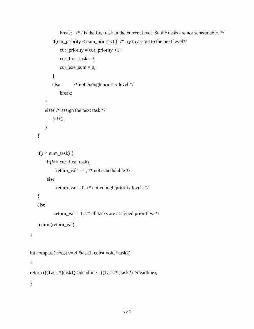
break; /* i is the first task in the current level. So the tasks are not schedulable. */

if(cur_priority < num_priority) { /* try to assign to the next level*/

cur_priority = cur_priority +1;

cur_first_task = i;

cur_exe_sum = 0;

}

else /* not enough priority level */

break;

}

else{ /* assign the next task */

i=i+1;

}

}

if(i < num_task) {

if(i== cur_first_task)

return_val = -1; /* not schedulable */

else

return_val = 0; /* not enough priority levels */

}

else

return_val = 1; /* all tasks are assigned priorities. */

return (return_val);

}

int compare( const void *task1, const void *task2)

{

return (((Task *)task1)->deadline - ((Task * )task2)->deadline);

}

C-4