DOT HS 809 050 April 2000 - NHTSA · PDF fileDOT HS 809 050 April 2000 ... blood alcohol content (BAC), drinking and driving, ... The objective of the present research is to re-examine

DOT HS 809 050 April 2000

RELATIVE RISK OF FATAL CRASHINVOLVEMENT BY BAC, AGE, AND GENDER

This document is available to the public from the National Technical Information Service, Springfield, VA 22161.

i

Technical Report Documentation Page1. Report No. 2. Government Accession No. 3. Recipient's Catalog No.

5. Report Date4. Title and Subtitle

Relative Risk of Fatal and Crash Involvement by BAC, Age and Gender6. Performing Organization Code

7. Author(s)

P.L. Zador, S.A. Krawchuk, R.B. Voas8. Performing Organization Report No.

10. Work Unit No. (TRAIS)9. Performing Organization Name and Address

Westat1650 Research BoulevardRockville, MD 20850

11. Contract or Grant No.

DTNH22-97-P-05174

13. Type of Report and Period Covered

Final Report12. Sponsoring Agency Name and Address

National Highway Traffic Safety AdministrationOffice of Research and Traffic Records400 7th Street, S.W., Washington, DC 20590

14. Sponsoring Agency Code

15. Supplementary Notes

Paul J. Tremont, Ph.D., was the Contracting Officer’s Technical Representative for this project.

16. Abstract

Objective: To re-examine and refine estimates for alcohol-related relative risk of driver involvement in fatal crashes by age andsex as a function of BAC using recent data.Methods: Logistic regression was used to estimate age/sex specific relative risk of fatal crash involvement as a function of theBAC of fatally injured and surviving drivers by combining crash data from the Fatality Analysis Reporting System withexposure data from the 1996 National Roadside Survey of Drivers.Results: In general, the relative risk of involvement in a fatal passenger vehicle crash increased steadily with increasing driverBAC in every age/sex group among both fatally injured and surviving drivers. A 0.02 percentage point BAC increase among16-20 year old male drivers was estimated to more than double the relative risk of fatal single vehicle crash injury. At the mid-point of the 0.08% - 0.10% BAC range, the relative risk of a fatal single-vehicle crash injury varied between 11.4 (drivers 35and older) and 51.9 (male drivers, 16-20). With only very few exceptions, older drivers had lower risk of being fatally injuredin a single vehicle crash than younger drivers, and females than males in the same age range. When comparable, results largelyconfirmed existing prior estimates.Conclusions: This is the first study that systematically estimated relative risk for drinking drivers with BACs between 0.08%and 0.10% (these relative risk estimates apply to BAC range mid-points at 0.09%). The results clearly show that drivers atnon-zero BACs somewhat below 0.10% pose highly elevated risk both to themselves and to other road users.

17. Key Words

relative risk, motor vehicle crash, motor vehicle fatality,blood alcohol content (BAC), drinking and driving,FARS, national survey, logistic regression, multipleimputation

18. Distribution Statement

19. Security Classif. (of this report) 20. Security Classif. (of this page) 21. No. of Pages 22. Price

Form DOT F 1700.7 (8-72) Reproduction of completed page authorized

THE PLAYER

April 2000

THE PLAYER

This report is available from the National Technical Information Service (NTIS), Springfield, VA 22161, tel. 703.605.6000, and from the NHTSA web site at www.nhtsa.dot.gov.

iii

Table of Contents

Section Page

1 Introduction and Background........................................................................... 12 Methods............................................................................................................ 23 Results .............................................................................................................. 54 Discussion ........................................................................................................ 95 References ........................................................................................................ 18

List of Appendices

A Weight adjustments to the exposure data ......................................................... AB Driver selection from FARS............................................................................. BC Logistic regression models............................................................................... CD Fay's method for generating replicate weights ................................................. DE Estimating design-based variances in the presence

of multiply imputed BACs ............................................................................... EF Alternative models logistic regression models for

involvement/exposure ratios............................................................................. F

iv

Table of Contents (continued)

List of Figures

Figure Page

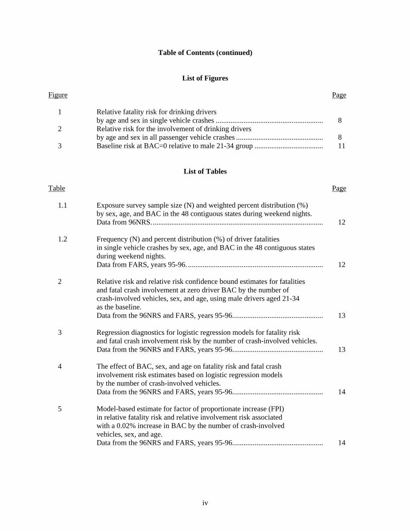
1 Relative fatality risk for drinking driversby age and sex in single vehicle crashes .......................................................... 8

2 Relative risk for the involvement of drinking driversby age and sex in all passenger vehicle crashes ............................................... 8

3 Baseline risk at BAC=0 relative to male 21-34 group ..................................... 11

List of Tables

Table Page

1.1 Exposure survey sample size (N) and weighted percent distribution (%)by sex, age, and BAC in the 48 contiguous states during weekend nights.Data from 96NRS............................................................................................. 12

1.2 Frequency (N) and percent distribution (%) of driver fatalitiesin single vehicle crashes by sex, age, and BAC in the 48 contiguous statesduring weekend nights.Data from FARS, years 95-96. ......................................................................... 12

2 Relative risk and relative risk confidence bound estimates for fatalitiesand fatal crash involvement at zero driver BAC by the number ofcrash-involved vehicles, sex, and age, using male drivers aged 21-34as the baseline.Data from the 96NRS and FARS, years 95-96................................................. 13

3 Regression diagnostics for logistic regression models for fatality riskand fatal crash involvement risk by the number of crash-involved vehicles.Data from the 96NRS and FARS, years 95-96................................................. 13

4 The effect of BAC, sex, and age on fatality risk and fatal crashinvolvement risk estimates based on logistic regression modelsby the number of crash-involved vehicles.Data from the 96NRS and FARS, years 95-96................................................. 14

5 Model-based estimate for factor of proportionate increase (FPI)in relative fatality risk and relative involvement risk associatedwith a 0.02% increase in BAC by the number of crash-involvedvehicles, sex, and age.Data from the 96NRS and FARS, years 95-96................................................. 14

v

Table of Contents (continued)

List of Tables (continued)

Table Page

6.1 Model-based relative driver facility risk and risk confidence boundestimates for single vehicle crashes by BAC, sex, and age, usingzero BAC as the baseline.Data from the 96NRS and FARS, years 95-96................................................. 15

6.2 Model-based relative driver involvement risk and risk confidencebound estimates for single vehicle crashes by BAC, sex, and age,using zero BAC as the baseline.Data from the 96NRS and FARS, years 95-96................................................. 15

6.3 Model-based relative driver fatality risk and risk confidence boundestimates for two vehicle crashes by BAC, sex, and age, usingzero BAC as the baseline.Data from the 96NRS and FARS, years 95-96................................................. 16

6.4 Model-based relative driver involvement risk and risk confidencebound estimates for two vehicle crashes by BAC, sex, and age,using zero BAC as the baseline.Data from the 96NRS and FARS, years 95-96................................................. 16

6.5 Model-based relative driver fatality risk and risk confidencebound estimates for all passenger vehicle crashes byBAC, sex, and age, using zero BAC as the baseline.Data from the 96NRS and FARS, years 95-96................................................. 17

6.6 Model-based relative driver involvement risk and risk confidenceestimates for all passenger vehicle crashes by BAC, sex, and age,using zero BAC as the baseline.Data from the 96NRS and FARS, years 95-96................................................. 17

1

1. Introduction and Background

According to National Highway Traffic Safety Administration (NHTSA) information, as of theend of September 1999, 31 states defined driving with a blood alcohol concentration (BAC) above 0.10%as a crime per se, while another 17 states plus the District of Columbia set their per se1 limit at 0.08%.Due to a combination of legal measures, enforcement actions, and changes in voluntary behavior patterns,alcohol-related fatalities have been declining for nearly two decades, both in absolute numbers and as aproportion of all fatalities. Nonetheless, there were still 15,936 alcohol-related traffic fatalities in theUnited States which accounted for nearly 38% of total traffic fatalities in 1998 (U.S. DOT, 1999)indicating that much more needs to be done.

Based on extensive research over several decades, we now have overwhelming evidence showingthat even BACs as low as 0.02% impair driving-related skills. One line of such evidence grows out oflaboratory research with dosed subjects (Moskowitz and Robinson, 1987; see also U.S. Department ofHealth and Human Services (HHS), 1997, Chapter 7). Confirming evidence comes from field researchthat compares the BACs of crash-involved with non-crash-involved drivers to determine the relative riskof crash involvement (Zador, 1991; see also Perrine et al., 1989, for a review). Two types of relative riskstudies have been conducted. “Classical” studies such as that of Borkenstein et al. (1974) used aprocedure in which data from non-crash-involved drivers were collected at the same times and locationsas the reference crash had occurred. This procedure was adopted in an effort to ensure that the onlypotential difference between the crash and non-crash driver would be the presence or absence of alcohol.An alternative survey procedure was employed by Zador (1991). He compared crash-involved driversfrom the National Highway Traffic Administration, Fatality Analysis Reporting System (FARS), withdata from the 1986 National Roadside Survey (NRS) (Wolfe, 1986). This procedure loses some of theprecision provided by using the site of the reference crash as the basis for selecting comparison cases.However, it gains reliability because it uses larger numbers and a broader representation that relates to thecountry as a whole, rather than to a single locality.

The selection of cases that define the crash-involved and non-crash-involved drivers bearssignificantly on the resulting risk curves. Clearly, many drivers are involved in crashes through no faultof their own but because of the mistakes of others. Therefore, it is important to consider responsibility inselecting the crash-involved drivers. This is generally accomplished by including only drivers in singlevehicle crashes (i.e., other drivers were not involved). Previous relative risk studies have demonstratedthat the relationship between BAC and crash risk is much stronger for drivers in single vehicle crashesthan for drivers in multiple vehicle crashes (Perrine et al., 1989; Zador, 1991). Three methods ofselecting comparison cases have been used in previous studies. As noted above, comparison drivers havebeen interviewed at crash sites (Borkenstein et al., 1974), through national roadside surveys (Zador, 1991;for overview, see also Chapter 10 in HHS, 1993) and through the selection of nonresponsible drivers inmultiple vehicle crashes — so called “induced exposure” (Hurst, 1974; Borkenstein et al., 1974). Hurst’sanalysis of nonresponsible drivers indicated that their crash risk curve was flat and did not increase withhigher BACs.

The objective of the present research is to re-examine and refine relative fatal crash risk estimatesin a systematic fashion using more recent data. The study was based on U.S. data on drivers in fatalcrashes during 1995 and 1996 obtained from the Fatality Analysis Reporting System (NHTSA, FARS),and driver exposure data obtained from the 1996 National Roadside Survey (Voas et al., 1997). It extendssimilar prior work by the first author in three important ways. Firstly, we estimate relative risk for thepolicy-relevant BAC range between 0.08% and 0.10%. Secondly, we estimate relative risk for six driver

1 A per se law defines it as a crime to drive with a BAC at or above the proscribed level.

2

groups: (1) Driver fatalities in single vehicle crashes, (2) Driver involvements in single vehicle fatalcrashes, (3) Driver fatalities in two vehicle crashes, (4) Driver involvements in two vehicle fatal crashes,(5) Driver fatalities in all crashes, and (6) Driver involvement in all fatal crashes. Thirdly, we employstatistical methods to estimate both the effect of sampling roadside exposure, and the effect of multipleimputation of missing BACs on the uncertainty of relative risk estimates.

2. Methods

Data Sources

Driver Exposure Data: the 1996 Roadside Survey

Following the same principles as its two predecessors in 1973 and 1986, the 1996 NationalRoadside Survey (96NRS) of weekend, nighttime drivers in the 48 contiguous states, interviewed andbreath-tested a sample of noncommercial operators of four-wheel vehicles during a roughly one monthperiod in the Fall of 1996. Counties with a population of less than 20,000 were not sampled, and incounties with larger populations, roadways with average daily traffic below 2,000 were excluded from thesurveys (for details, see Lestina et al., 1999). Drivers were selected for interviews and breath tests using ageographically stratified multi-stage cluster sample. This survey was designed based on the NationalAutomotive Sampling System/Crashworthiness Data System (NASS/CDS, 1995). The first stage of thedesign comprised 24 Primary Sampling Units (PSUs) employed by NASS/CDS, six each in the Northeast,South, West, and Midwest. Only the section of the NASS PSUs appropriate for the 48 states wereemployed in the 1996 sampling plan. The second stage comprised a total of 46 police jurisdictions, 11-12per region. At the third stage, square grids with sides roughly equal to one mile were superimposed onthe sampled jurisdictions, and then randomly sampled to obtain the requisite number of squares (thisprocedure was modified for areas with low road density). Once a square was chosen, the survey wasconducted at the first safe area found in it by the survey team leader. Driver selection represented thefinal stage: the first driver who approached the site after an interviewer became available was stopped forthe next interview. Field operations were conducted on Friday and Saturday nights during two two-hourperiods at separate sites, at one site between 10 PM and midnight, and at the other between 1 AM and 3AM. Data from the 96NRS is representative only of locations and periods when drinking and driving ismost prevalent (i.e., not all times or roadways in the 48 contiguous states).

Data from 96NRS were used to estimate the approximate distribution of driver exposure by sex,age (16-20, 21-34, and > 35), and BAC (0.000, 0.001-0.019, 0.020-0.049, 0.050-0.079, 0.080-0.099,0.100-0.149, and 0.150+). Specifically, we approximated the statistical distribution of drivers onweekend nights using the distribution of driver sampling weights after adjustments for nonrespondents(see Appendix A).

Data on Drivers in Fatal Crashes

The Fatality Analysis Reporting System (FARS) is a census of all motor vehicle crashes thatoccur on a public trafficway in the United States and result in a fatality within 30 days. Although FARSis maintained by NHTSA of the U.S. Department of Transportation, the data in FARS are obtainedthrough cooperative agreements with agencies in each state's government, and are managed by RegionalContracting Officer’s Technical Representatives located in the ten NHTSA Regional Offices. For basicdata elements associated with a fatal motor vehicle crash, reporting is usually of very high quality withrelatively few missing values with one exception: even in recent years, BACs were not available for manydrivers involved in fatal crashes. To deal with this problem, NHTSA has employed a statistical methodfor imputing missing BACs since the early 1980s, (Klein, 1986). More recently, the method of multiple

3

imputation (Rubin, 1987) was adopted to handle the problem of missing BACs on FARS (Rubin et al.,1999). Under multiple imputation, each missing value is replaced by a small number of imputed values(10, in the present case) which are generated by a statistical procedure designed to reflect the statisticalproperties of the missing driver BACs. We used the ten complete-data versions of FARS in our statisticalanalyses. Note that while the data files for the multiple imputation method are available, NHTSA is notyet using the multiple imputation method for its published alcohol estimates. The same method used inprevious years is to be used for the 1998 FARS estimates.

We classified drivers of four-wheel passenger vehicles involved in fatal crashes during 1995 or1996 by the number of crash-involved vehicles (one, two, and any number (one, two, or more) ofvehicles) and by whether or not the driver was just involved in the crash, or was also fatally injured in thecrash. We thus defined six driver groups for analysis: drivers fatally injured in single vehicle crashes,drivers involved in fatal single vehicle crashes, drivers fatally injured in two vehicle crashes, driversinvolved in fatal two vehicle crashes, drivers fatally injured in a crash, and drivers involved in a fatalcrash. We then screened drivers using criteria that approximately matched the criteria for selecting theexposure sample. We included drivers of passenger vehicles involved in crashes during weekend nightsand excluded crashes that occurred on interstates, other urban freeways, and expressways (for additionaldetails, see Appendix B). There were only two notable differences between the exposure and the crashscreening criteria, and both were disregarded to increase the sample size for drivers retained for theanalyses. First, we accepted crashes that occurred between midnight and 1 AM, since those crashes wereexcluded from the exposure sample only to permit the survey team to change location, and not becauseBAC distribution between midnight and 1 AM was thought to be different. Second, we did not restrictcrashes to the weekend nights during which the surveys were conducted. Including weekend nights forthe whole year increased sample sizes almost 12-fold, and introduced no substantial difference in thedistribution of driver BACs since driver BACs varied little between the survey period and the rest of theyear.

We classified the six groups of driver fatalities and involvements in the same way as we classifiedthe exposure sample, by sex, age (16-20, 21-34, and > 35), and BAC (0.000, 0.001-0.019, 0.020-0.049,0.050-0.079, 0.080-0.099, 0.100-0.149, and 0.150+).

Statistical Methods

Using Odds Ratios and Logistic Regression to Estimate Relative Risk

Following Zador (1991), we base our methods on the intuitive notion that comparisons betweenthe frequency distribution of fatal crash involvement by sex, age and BAC and the frequency distributionof roadside exposure by sex, age, and BAC can provide a good yardstick for measuring the effect of thesefactors on the relative likelihood of fatal crash involvement per unit of driving exposure. Since the96NRS did not provide a national estimate for total miles driven on weekend nights, it was not possible toscale fatal involvement and exposure count ratios to the corresponding involvement rates per milesdriven. However, since our involvement (or fatality) count per exposure ratios are proportional tonational involvement (or fatality) rates, dividing two such ratios, say at different BACs, gives thecorresponding ratio of involvement (or fatality) rates. Thus, data on fatal involvement from FARS anddriving exposure from 96NRS can be used to estimate involvement per exposure ratios which, in turn,effectively approximate relative crash risk.2

2 For a general discussion of relative risk, see Schlessellman, J.J. Case-Control Studies: Design, Conduct and Analysis. New York: Oxford

University Press, 1982.

4

More specifically, consider a two way table formed of fatality and (weighted) survey counts fortwo populations (group 1 and group 2):

Population Fatality Count Exposure Count

Group 1 F1 E1

Group 2 F2 E2

The odds ratio:

Odds Ratio = (F1/E1)/(F2/E2) (1)

compares the fatality/exposure ratio between groups 1 and 2. Taking group 2 as the baseline, this oddsratio compares fatality odds in group 1 to fatality odds in group 2. Odds ratios (OR) being scale invariant,we can substitute cE1 and cE2 in (1) for exposure counts E1 and E2, where c is the scaling constant,without affecting the numeric value of the OR. Now, for a large value of c, the odds in the numerator andthe denominator of (1) have approximately the same value as the corresponding crash rates: F1/(F1+cE1)and F2/(F2+cE2). The unknown value of c that would scale up survey-based exposure counts to thenational total of miles driven is extremely large relative to observed involvement/exposure ratios.Therefore, it is legitimate to use the odds ratios (F1/E1)/(F2/E2) to estimate relative risk,F1/(F1+cE1)/F2/(F2+cE2). Given this discussion, and following the common practice in epidemiology,3

we used odds ratios to estimate relative risk, and henceforth we will refer to estimates of relative risk,rather than to estimates of odds ratios.

We used logistic regression4 to model involvement (or fatality) counts relative to exposurecounts, and performed two sets of analyses for each of our six driver sets. In the first set (results arefound in Table 2), we estimated relative risk among drivers with zero BAC by age and gender. In thesemodels, we chose male drivers between ages 21 and 34 for baseline, and estimated relative involvementrisk for the other five driver groups. In the second set (results in Table 6.1 - 6.6), we estimated relativerisk as a function of driver BAC within sex and age groups. In the latter models, drivers with BAC = 0were chosen as baseline. Note that any non-significant interaction terms were not retained in the finalmodel. For both analyses, in addition to relative risk, we also estimated lower and upper confidencebounds for relative risk.

We estimated relative risk by exponentiating model parameter estimates for the effect of BAC fordriver groups of interest. The formula for relative risk (RR) associated with a BAC value was,RR(BAC) = exp(b BAC), where b denotes the regression coefficient estimate for a BAC variable.Similar other formulae are given in Appendix C for estimating lower/upper bounds for relative risk.

Model Performance

We assessed model performance using four statistics: 1) the heterogeneity factor estimated as thePearson chi-square statistic divided by its degrees of freedom, 2) the maximum of rescaled R2, 3) theHosmer-Lemeshow goodness-of-fit test p-value, and 4) the Wilk-Shapiro statistic p-value for testing the

3 For a general discussion of relative risk, see Schlessellman, J.J. Case-Control Studies: Design, Conduct and Analysis. New York: Oxford

University Press, 1982.

4 Logistic regression was implemented using the SAS procedure, Proc Logistic (SAS Institute, Inc. 1996).

5

normality of standardized Pearson residuals. For data that are conditionally binomial, the dispersionparameter is approximately equal to 1. A heterogeneity factor substantially larger than one is indicativeof overdispersion that is, more variation than would be expected under the assumption thatconditionally on the sum of exposure and fatality counts, the fatalities were binomially distributed. Weadjusted all variance and confidence bounds for the presence of overdispersion. The maximum rescaledR2 (Nagelkerke, 1991) can be used to assess model quality somewhat in the manner of the customary R2

statistic for linear regressions. The Hosmer-Lemeshow test statistic is a direct measure for a logisticregression model's ability to predict outcome probabilities (Hosmer and Lemeshow, 1989). We haveapplied the Wilk-Shapiro test to determine whether standardized residuals followed an approximatenormal distribution. In the ideal case, heterogeneity factor and rescaled R2 are near one, and the p valuesare between 0.05 and 0.95.

Variance Estimation

As described earlier, the 1996 National Roadside Survey had a complex, multi-stage design. Ifno special steps were taken, standard statistical packages would tend to underestimate true variability fordata collected under a complex design. We used Fay’s method of balanced repeated replications (BRR)to obtain design-consistent variance estimates for important model parameters. This involved three steps.First, we used Westat’s implementation of Fay’s method (WesVarPC, 1998) to create replicate weightsfrom the adjusted full-sample weight (see Appendix D). Second, we repeatedly estimated our modelsusing the full-sample weight, and each set of replicate weights. Finally, we combined the resultingestimates using a simple formula to obtain design-unbiased variance estimates (see Appendix E).

As part of data preparation, NHTSA had replaced missing driver BACs on FARS by ten imputedBAC values (Rubin et al., 1999). On the one hand, having imputed values on FARS made it possible toemploy complete-data methods in our analyses. On the other hand, unless special care is exercised, usingimputed values as if they were actual values would result in underestimating variability (Rubin, 1987).We followed Rubin’s two-step method to eliminate this bias. In Step 1, we re-estimated our models usingeach of the ten imputed BAC values and averaged the results. In Step 2, we combined the 10 sets ofestimates into one single unbiased variance estimate (see Appendix E). Since there were 12 replicateweights for exposure and 10 multiply-imputed completed sets of driver counts, we estimated modelparameters for each of the six driver populations a total of 130 times in order to compute imputation-adjusted and design-consistent parameter variances

3. Results

According to Table 1.1, about 84% of the weighted drivers in the exposure sample had a zeroBAC, about 9.2% had a non-zero BAC under 0.05%, 4.7% had a BAC between 0.05% and 0.1%, 2.1%had a BAC between 0.1% and 0.15%, and only 0.6% of the weighted roadside sample had a BAC over0.15%. Overall, males accounted for about 65% of all exposure. Drivers between 21 and 34 years of ageand drivers over 34 years of age were represented roughly in equal proportions among both males andfemales. Drivers 16-20 accounted for about half the exposure of the other two age groups amongfemales, but less than half among males.

For all six driver involvement groups, driver BAC distributions differed strikingly from thecorresponding exposure distribution in every sex-age group, as shown by comparing Table 1.1 to Table1.2. Even among sober drivers (i.e. BAC = 0), striking differences were found in involvement/exposureratios across sex and age groups, as indicated in Table 2. Taking the risk of being killed in a singlevehicle crash to be 1.00 for sober male drivers 21-34, the comparable risk was 1.75 for sober male drivers16-20, and it was 0.71 for sober male drivers over age 34. In every age group, sober female drivers had a

6

lower risk of being killed in a single vehicle crash than sober male drivers, with relative risks decreasingfrom 1.18, among the youngest group of females, to 0.28 among the oldest group. Note that controllingfor sex, confidence intervals for adjacent age groups did not overlap (except for the two highest age groupfemales), and controlling for age groups, the confidence intervals for males and females, did not overlap(except for the youngest age group). Thus, most sex and age group related differences in single vehicledriver fatality rates were not attributable to chance variation. Note that the distributions of fatally injureddrivers for each driver involvement group are available from the first author.

Sex and age affected a driver's relative risk of being involved in a fatal single vehicle crash inmuch the same way as it affected the driver's relative risk of being killed in one. In contrast, Table 2shows that the pattern of results differed markedly for two vehicle crashes from the pattern of results forsingle vehicle crashes, especially for females. First, although relative risk still decreased with increasingage among males, the differences were smaller for two vehicle crashes than for single vehicle crashes.Moreover, relative involvement risk was lower for sober 21-34 females than for any of the two otherfemale age groups, but the confidence intervals overlapped for females. Also, the relative fatality risk ofsober females 35 and over exceeded the relative fatality risk of sober males 21-34.

Tables 3, 4, 5, and the Table 6 series, present selected model diagnostics, logistic regressionmodel parameter estimates and standard errors, model-based estimates of proportionate increase inrelative involvement risk and fatal injury risk associated with a 0.02% increase in BAC, and model-basedrelative risk estimates with their confidence intervals, respectively. Models in Table 4 include nineparameters.

1. Indicator variables (N = 3) for AGE groups: 16-20, 21-34, and > 34,2. Indicator variable for being female,3. Indicator variable for interaction term involving low positive BAC (0.001%-0.019%) among

drivers > 20 ,4. Continuous variables (interaction terms) (N = 3) for the effect of BAC by age group: 16-20,

21-34, and > 34,5. Continuous variable (interaction term) for the effect of BAC for females 16-20.

As evidenced by the results of the Hosmer-Lemeshow goodness-of-fit test and the Shapiro-Wilktest for the normal distribution of standardized Pearson residuals, relative risk was adequately representedby the models in Table 4 for three of the driver groups: drivers involved in a fatal single vehicle crash,drivers killed in a single vehicle crash, and drivers killed in any crash (see Table 3). These modelsaccounted for substantial percentages of the explainable variation: 68% among drivers killed in a singlevehicle crash, 53% among drivers killed in any crash, and 49% among drivers involved in a fatal singlevehicle crash. These data also exhibited statistically significant, but relatively modest heterogeneity.While the Hosmer-Lemeshow test statistic (p = 0.032) rejected the hypothesis of model fit for fatallyinjured drivers in two vehicle crashes, the regression model explained 65% of all explainable relative riskvariation, and the standardized Pearson residuals were normally distributed. All-in-all, we deem model fitacceptable for driver fatalities in two vehicle crashes. In contrast, the models performed poorly for thetwo remaining driver groups drivers in fatal crashes involving two vehicles or drivers in fatal crashesinvolving any number of vehicles. Specifically, both Hosmer-Lemeshow test statistics rejected thehypothesis of model fit, both models explained only about 30% of the explainable relative risk variation,both heterogeneity factors were over 3, and even the residuals were not normally distributed for drivers infatal crashes involving any number of vehicles.

7

We explored the way our models broke down for fatal two vehicle crashes in considerable detail.We examined model fit statistics for the models in Table 4, and for several other model specifications,5

including specifications obtained by stepwise regression. The results clearly showed that sober driverinvolvement in two vehicle crashes is not closely related to driver involvement at positive BACs, and wediscovered that only the inclusion of indicator variables representing overall sober driver risk, and soberdriver risk by age and gender, would produce acceptable model fit. This result was, in fact, not toosurprising for two reasons. First, in crashes involving more than a single vehicle, some driver(s) may beinnocent, and probably sober, victim(s) whose vehicle(s) were struck by a high BAC at-fault driver.Secondly, in multi-vehicle crashes, crash configuration and vehicle occupancy become importantdeterminants of relative risk. However, we decided not to use regression models that included soberdriver risk variables (e.g., main effect for zero BAC, zero BAC by age interaction, etc., see Appendix F)because it was not clear how these models can be used to estimate relative risk with BAC = 0 as thebaseline. Therefore, relatively poor model fit notwithstanding, we believe that the relative risk estimatespresented from the model parameter estimates in Table 4 provide reasonable, albeit conservative,approximations of the true relative risk even for driver involvement in multi-vehicle fatal crashes.Additional research will be needed to improve model fit for these driver groups.

We computed relative risk as a function of BAC from one or more regression coefficients relativeto sober driver risk, that is relative to the risk of drivers with 0.0% BAC (for positive BACs, we re-scaledpercent BAC by a factor of a 1000 so that 0.1% was entered in formulas as 100). For example, therelative risk of receiving a fatal injury in a single vehicle crash by a driver 21-34 whose BAC is 0.13%was estimated at RR(0.13) = exp(0.029 x 130) = 43.4, where 130 = 0.13 x 1000, and b = 0.029 is theregression coefficient from Table 4 for the parameter “BAC, Age 21-34”. In other words, among drivers21-34, a BAC of 0.13% increased the chance of being killed in a single vehicle crash by a factor of about43. Table 5 shows model-based estimates for factor of proportionate increase in relative risk associatedwith an increase of 0.02% in BAC level for each driver group, by age and sex. Of noteworthy mention, itwas estimated that each 0.02 percentage point increase in the BAC of a driver with a non-zero BAC morethan doubled the risk of receiving a fatal injury in a single vehicle crash among male drivers 16-20, andnearly doubled the comparable risk among the other driver groups. Proportionality factors were estimatedfrom age-specific regression coefficients of BAC in Table 4 except that for female drivers 16-20, theestimates were adjusted for the effect of being female. For the relative risk estimates in subsequenttables, relative risk was also adjusted for the effect of low BAC (0.001% - 0.019%) for drivers 21 orolder. For the purpose of fitting models, we represented BAC class intervals (by sex and age) by averagedriver BAC. However, to facilitate comparisons across driver populations, we present relative riskestimates at constant BACs (0.0%, 0.01%, 0.035%, 0.065%, 0.090%, 0.125%) that correspond to classinterval midpoints for the first five BAC categories, and 0.220% for the last BAC category, whichcorresponds to the average BAC of those with BAC values greater than 0.15%.

The relative risk of receiving a fatal injury in a single vehicle crash increases steadily withincreasing driver BAC for both males and females in every age group with one exception (see Figure 1and Table 6.1). Among all male and female drivers, except those in the 16-20 group, the relative risk ofreceiving a fatal injury is lower for drivers with a positive BAC under 0.02% than for drivers with 0.0%BAC. Remarkably, however, for the 16-20 age group, the comparable relative risk was substantiallyincreased even at this low positive BAC, by 55% among males, and by 35% among females. Looking atrelative risk across the six age and gender groups, we find that at a BAC of 0.035%, it was elevated by afactor between 2.6 and 4.6, at a BAC of 0.065%, by a factor between 5.8 and 17.3, at a BAC of 0.09%, bya factor between 11.4 and 52, at a BAC of 0.125%, by a factor between 29.3 and 240.9, and at a BAC of0.220%, by a factor between 382 and 15,560. Figure 1 indicates that relative risk increased fastest for

5 Dozens of other models were examined; for a few, results are summarized in Appendix F.

8

males 16-20, and slowest for drivers of either sex 35 and over. In general, controlling for age, relativerisk increased faster for males than for females, and controlling for sex, it increased faster for drivers 16-20 and slowest for drivers 35 and over. In addition, in every comparison, relative risk increased fasterwith increasing BAC for fatally injured drivers than for driver involvement in fatal crashes.

Figure 1. Relative fatality risk for drinking drivers by age and sex in single-vehicle crashes6

In general, the pattern of results for the other driver groups was quite similar to the pattern justdescribed (see Tables 6.2 - 6.6). Figure 2 and Table 6.6 show a similar pattern for driver involvement inall fatal crashes. The following represent major differences among the other driver groups. (1) Forfatally injured drivers, relative risk increased slower with increasing BAC in two vehicle than in singlevehicle crashes. As indicated earlier, this was to be expected since in multi-vehicle fatal crashes, someinvolved drivers were likely to be no more than marginally at-fault. (2) Also, since most fatally injureddrivers were killed in a single vehicle or in a two vehicle crash, the overall rate of increase in relative riskwas between the rates of increase for single vehicle and two vehicle crashes.

Figure 2. Relative risk for the involvement of drinking drivers by age and sex in all passenger vehiclecrashes7

6 BAC values are the midpoints of the intervals depicted in Table 6.1.

Risks off scale for BAC = 0.220: 16-20 Male = 15,560; 16-20 Female = 738;21-34 All = 573; 35+ All = 382.

Risk off scale for BAC = 0.125 16-20 Male = 241.Risk off scale for BAC = 0.090 16-20 Male = 52.

7 BAC values are the midpoints of the intervals depicted in Table 6.6.Risks off scale for BAC = 0.220: 16-20 Male = 2,372; 16-20 Female = 74;

21-34 All = 88; 35+ All = 84.Risk off scale for BAC = 0.125 16-20 Male = 83.

0

10

20

30

40

50

0 .0 0 0 0 .0 1 0 0 .0 2 0 0 .0 3 0 0 .0 4 0 0 .0 5 0 0 .0 6 0 0 .0 7 0 0 .0 8 0 0 .0 9 0 0 .1 0 0 0 .1 1 0 0 .1 2 0 0 .1 3 0

BAC

Rel

ativ

e fa

talit

y ri

sk

16-20 Male

16-20 Female

21-34 All

35+ All

0

10

20

30

40

50

0 .000 0 .010 0 .020 0 .030 0 .040 0 .050 0 .060 0 .070 0 .080 0 .090 0 .100 0 .110 0 .120 0 .130 0 .140 0 .150 0 .160 0 .170 0 .180 0 .190 0 .200 0 .210 0 .220

BAC

Rel

ativ

e ri

sk

16-20 Male 16-20 Female 21-34 All 35+ All

9

4. Discussion

Confirmatory Findings

This study has confirmed that, in general, relative risks of fatal injury and fatal crash involvementboth steadily increased with increasing driver BAC within each of the six driver age and sex groupsstudied. The only exception was that among drivers 21 and over, relative risk was lower at near-zeropositive BAC than at zero BAC. The classical Grand Rapids study by Borkenstein et al. (1974) found asimilar “dip” in the risk curve. Hurst (1973) showed that controlling self-reported drinking frequencyeliminates the Grand Rapids dip. The customary interpretation of these results is that the anomalous dipprobably results from differing alcohol tolerance between crash-involved and non-crash involved drivers.Since drinking frequency data were not available in our study, we were unable to estimate risk curves bydrinking frequency. With few exceptions, relative risk was found to decrease with increasing driver ageat every BAC level, both for males and for females a finding that extends similar age trends reportedfor moderate BACs by Zador (1991).

The current study also confirms the substantially higher relative risk for involvement in a singlevehicle crash of young drivers at a zero BAC previously reported by Mayhew et al. (1986). Overall,young drivers experienced higher relative risks of single vehicle crashes than did older drivers of the samesex. Additionally, female drivers exhibited substantially lower relative risk than male drivers of the sameage. To a somewhat lesser extent, both sets of findings were also true for most of the other five drivergroups studied.

In this study, lower and upper 95% confidence bound estimates for relative risk as a function ofdriver BAC take into account both the sampling variation of the roadside driver exposure sample, and theeffect of multiple BAC imputations performed by Rubin et al. (1999) for NHTSA. Not surprisingly,relative risk confidence intervals are wide. For example, lower and upper confidence bounds were 16.5and 164 for male drivers 16-20 killed in single vehicle crashes with a BAC between 0.08% and 0.10%.8

We note that the width of 95% confidence intervals increases with increasing BACs for mathematicalreasons.9 We also note that allowing for comparable variation in prior estimates, the relative riskestimates presented here are largely in line with estimates published elsewhere.10

New Findings

This is the first study that estimated relative risk from compatible data sources using the samemethods for six driver groups of interest defined by the number of crash-involved vehicles and, whetherthe driver was just involved, or also fatally injured in the crash. Drivers killed in single vehicle crashesare of particular interest for assessing the pure effect of drinking and driving because in single vehiclecrashes: driver fault is not shared, crash configuration is less of a factor, vehicle occupancy is notrelevant, and the seating position of the fatally injured occupant is fixed. In two vehicle crashes, thepossibility that fault may be split between two drivers, one or both of whom may have a (possiblydifferent) positive BAC, would seem to make it difficult to estimate the pure effect of BAC on crash risk.It was all the more gratifying to find the relative risk of a fatal driver injury depend on driver BAC in

8 These relative risk estimates apply to BAC range mid-points at 0.09%.

9 Both relative risk and its confidence bounds depend exponentially on the corresponding logistic regression parameters.

10 Relative risk estimates in this paper differ in several ways from similar estimates in Zador (1991). In the former study, the baseline BAC groupwas defined to include drivers at or below a BAC of 0.01%, age groups and BAC groups were defined differently, driver fatalities wereincluded from only 29 states with low rates of missing BACs, missing BACs were not imputed, and the numeric BAC values were not used inanalyses except to classify drivers.

10

almost the same way for single vehicle crashes as for two vehicle crashes provided that the relative riskmodel of two vehicle crashes statistically accounted for the possible roles of not at-fault sober drivers (seeAppendix F). In this study, we focused on the general effect on relative risk of a positive driver BAC,rather than on its pure effect. Our main statistical model for estimating relative risk did not, therefore,adjust relative risk estimates for the over-representation of sober (probably not-at-fault) drivers.Consequently, the model we used in this study appears to have generally underestimated the pure effect ofpositive driver BAC on relative risk, except for drivers in single vehicle crashes.

As noted earlier, this study confirmed that relative risk and driver age are inversely related atevery BAC. However, somewhat surprisingly in part contrary to Zador (1991), relative risk was found tobe generally lower at all BAC levels for females than for males for the 16-20 group. This lower relativerisk (roughly comparable to adult drivers 21 to 34 at BACs of 0.02% and over) is important because ofthe increasing incidence of drinking females in that age group in the nighttime driving populationobserved in the 96NRS. In that most recent survey, there were more, but not significantly more, womendrinking drivers in the 16-20 age group than males. Perhaps the lower relative risk could attributed tofemales driving more cautiously than their male age counterparts.

Finally, this study is the first that systematically estimated relative risk for drinking drivers withBACs between 0.08% and 0.10%,11 and the relative risk estimates obtained here provide clear evidencethat drinking and driving at BACs under 0.10% is very dangerous. For driver fatalities in single vehiclecrashes with a BAC in this range, relative risk estimates ranged from a low of 11.4 for drivers 35 andover, to a high of 51.9 for male drivers under 21, and even the lowest among the six lower confidencebounds indicated a nearly six fold rise in fatality risk. This similar pattern was also found overall (i.e., forany involvement in a fatal motor vehicle crash), although with smaller magnitudes. Drivers 35 and overhad the lowest relative risk of involvement at about 6.1, followed by those in the 21-34 age group at 6.3.The youngest male age group had a relative risk of about 24 – four times that of the other age groups(Table 6.6 and Figure 2). Naturally, relative risk was considerably higher for drivers with a BAC between0.10% and 0.15%, and ranged between 29 for drivers 35 and over and 241 for male drivers under 21 fordriver fatalities in single vehicle crashes. Relative risk for drinking drivers with a BAC at or above 0.15%ranged from 382 for drivers 35 and over, to 15,560 for male drivers under 21.

Policy Implications

There is considerable evidence that lowering state BAC limits to 0.08% from 0.10% reduced fatalmotor vehicle crashes (e.g., Hingson et al., 1996; Voas and Tippetts, 1999), and according to recentNHTSA information, 17 states plus the District of Columbia defined a driver BAC of 0.08% as illegal perse. New findings from this study lend support to lowering the illegal per se limit by showing that drivingat BACs under 0.10% is indeed very dangerous. Additionally, an ongoing laboratory investigation at theSouthern California Research Institute with participation by the first author of this study, has providedstrong evidence that impairment of driving-related performance occurs at very low BAC levels evenamong experienced drinkers.

Obviously, baseline differences are important for comparing driver groups in absolute terms sinceoverall crash risk is affected both by baseline risk differences among sober drivers, and by age- and sex-related differences in the effects of drinking and driving. For example, when considering policy optionsfor young drivers, it is important to bear in mind overall risk, not just sober-driving or drinking anddriving risks. Since young male drivers in the 16-20 age group start from an already high baseline risklevel in all driver groups (see Figure 3), even at slightly elevated BACs in the 0.02% - 0.05% range, this

11 These relative risk estimates apply to BAC range mid-points at 0.09%.

11

group experienced fatal driver injuries in single vehicle crashes more than eight times as often as sobermale drivers 21-34. Policy measures designed to reduce drinking and driving and alcohol-related crashesin the youngest age group include the enforcement of minimum drinking age laws that prohibit thepurchase of alcoholic beverages by persons under age 21, and the establishing and enforcing of near-zeroBAC limits (zero tolerance) for drivers under 21. Complementary strategies designed to reduce bothsober-driving and drinking and driving crashes among the youngest drivers include graduated licensureand young curfews (U.S. DOT, 1998).

Figure 3. Baseline risk at BAC=0 relative to male 21-34 group

With the new findings of this study, and parallel results currently being observed in laboratorystudies at the Southern California Research Institute, one can state with confidence that driving at non-zero BACs somewhat lower than 0.10% is indeed very dangerous. Thus, reducing BAC limits from0.10% to 0.08% is an effective method of saving lives. Moreover, these results show that with suchelevated relative risks, reducing drinking and driving at any BAC level is likely to further reduce alcohol-related motor vehicle fatalities in the United States.

0

0.2

0.4

0.6

0.8

1

1.2

1.4

1.6

1.8

2

M F M F M F

Rel

ativ

e R

isk

Fatalities,Single Vehicle CrashesInvolvement,All Crashes

16-20 21-34 35+

12

Table 1.1. Exposure survey sample size (N) and weighted percent distribution (%) by sex, age, andBAC in the 48 contiguous states during weekend nights.Data from 96NRS.

BAC

000 001-019 020-049 050-079 080-099 100-149 150+Total

Sex Age N % N % N % N % N % N % N % N %

Male 16-20 566 9.9 16 0.3 26 0.2 10 0.1 5 0.2 1 0.0 1 0.0 625 10.6

21-34 1,279 19.0 97 1.4 139 1.7 105 1.7 34 0.4 70 1.0 25 0.3 1,749 25.4

35+ 1,292 24.0 86 1.4 90 1.4 44 0.6 31 0.3 32 0.6 19 0.3 1,594 28.5

All 3,137 52.9 199 3.0 255 3.3 159 2.3 70 0.9 103 1.6 45 0.5 3,968 64.6

Female 16-20 303 6.6 7 0.1 7 0.3 6 0.2 3 0.0 3 0.0 0 0.0 329 7.2

21-34 617 11.9 32 0.5 72 0.9 37 0.6 15 0.2 18 0.3 3 0.0 794 14.4

35+ 643 12.1 27 0.5 28 0.6 12 0.2 8 0.2 10 0.2 1 0.0 729 13.7

All 1,563 30.6 66 1.1 107 1.7 55 0.9 26 0.5 31 0.5 4 0.0 1,852 35.4

All 16-20 869 16.5 23 0.4 33 0.5 16 0.3 8 0.2 4 0.0 1 0.0 954 17.9

21-34 1,896 30.9 129 1.9 211 2.6 142 2.3 49 0.7 88 1.2 28 0.3 2,543 39.8

35+ 1,935 36.1 113 1.9 118 1.9 56 0.7 39 0.5 42 0.8 20 0.3 2,323 42.3

All 4,700 83.5 265 4.1 362 5.1 214 3.3 96 1.4 134 2.1 49 0.6 5,820 100.0

Table 1.2. Frequency (N) and percent distribution (%) of driver fatalities in single vehicle crashes bysex, age, and BAC in the 48 contiguous states during weekend nights.Data from FARS, years 95-96.

BAC

000 001-019 020-049 050-079 080-099 100-149 150+Total

Sex Age N % N % N % N % N % N % N % N %

Male 16-20 113 4.4 3 0.1 21 0.8 27 1.1 26 1.0 89 3.5 156 6.1 435 17.0

21-34 124 4.9 1 0.0 15 0.6 41 1.6 41 1.6 200 7.8 619 24.3 1,041 40.8

35-97 111 4.3 0 0.0 11 0.4 16 0.6 17 0.7 84 3.3 420 16.5 659 25.8

All 348 13.6 4 0.2 47 1.8 84 3.3 84 3.3 373 14.6 1,195 46.8 2,135 83.7

Female 16-20 51 2.0 3 0.1 4 0.2 6 0.2 2 0.1 11 0.4 15 0.6 92 3.6

21-34 33 1.3 0 0.0 2 0.1 11 0.4 10 0.4 36 1.4 99 3.9 191 7.5

35-97 22 0.9 0 0.0 3 0.1 4 0.2 6 0.2 15 0.6 84 3.3 134 5.3

All 106 4.2 3 0.1 9 0.4 21 0.8 18 0.7 62 2.4 198 7.8 417 16.3

All 16-20 164 6.4 6 0.2 25 1.0 33 1.3 28 1.1 100 3.9 171 6.7 527 20.7

21-34 157 6.2 1 0.0 17 0.7 52 2.0 51 2.0 236 9.2 718 28.1 1,232 48.3

35-97 133 5.2 0 0.0 14 0.5 20 0.8 23 0.9 99 3.9 504 19.7 793 31.1

All 454 17.8 7 0.3 56 2.2 105 4.1 102 4.0 435 17.0 1,393 54.6 2,552 100.0

13

Table 2. Relative risk and relative risk confidence bound estimates for fatalities and fatal crashinvolvement at zero driver BAC by the number of crash-involved vehicles, sex, and age,using male drivers aged 21-34 as the baseline.Data from the 96NRS and FARS, years 95-96.

Number of vehicles in fatal crashSingle vehicle Two vehicle Any

Injury Injury InjurySex Age Fatal Involv. Fatal Involv. Fatal Involv.Male 16-20 Relative risk 1.75 1.89 1.44 1.23 1.52 1.48

Lower 1.33 1.58 1.05 1.02 1.23 1.29Upper 2.30 2.27 1.98 1.48 1.88 1.71

21-34 Relative risk 1.00 1.00 1.00 1.00 1.00 1.00Lower 1.00 1.00 1.00 1.00 1.00 1.00Upper 1.00 1.00 1.00 1.00 1.00 1.00

35+ Relative risk 0.71 0.61 0.90 0.69 0.81 0.67Lower 0.54 0.51 0.68 0.59 0.67 0.59Upper 0.93 0.73 1.19 0.82 0.98 0.76

Female 16-20 Relative risk 1.18 1.04 0.89 0.80 1.02 0.91Lower 0.83 0.82 0.58 0.63 0.78 0.76Upper 1.67 1.32 1.35 1.01 1.33 1.08

21-34 Relative risk 0.43 0.63 0.67 0.59 0.57 0.65Lower 0.29 0.51 0.46 0.48 0.44 0.56Upper 0.63 0.79 0.98 0.73 0.75 0.76

35+ Relative risk 0.28 0.39 1.10 0.69 0.62 0.58Lower 0.18 0.31 0.80 0.56 0.48 0.49Upper 0.44 0.51 1.51 0.84 0.80 0.68

Table 3. Regression diagnostics for logistic regression models for fatality risk and fatal crashinvolvement risk by the number of crash-involved vehicles.Data from the 96NRS and FARS, years 95-96.


Injury Injury InjuryDiagnostic Fatal Involv. Fatal Involv. Fatal Involv.Heterogeneity factor 1.6979 1.7774 1.8783 3.3159 2.0918 3.7070Max-rescaled rsquare 0.6844 0.4935 0.6524 0.3142 0.5297 0.3171H-L goodness-of-fit, p 0.1998 0.6806 0.0317 0.0001 0.4008 0.0002Normality of residuals, p 0.2813 0.0606 0.5701 0.4175 0.2189 0.0165

14

Table 4. The effect of BAC, sex, and age on fatality risk and fatal crash involvement risk estimatesbased on logistic regression models by the number of crash-involved vehicles.Data from the 96NRS and FARS, years 95-96.


Injury Injury InjuryParameter Fatal Involv. Fatal Involv. Fatal Involv.Age 16-20 Regression coefficient -1.547 -0.572 -2.184 -0.873 -1.077 0.085

Standard error of R.C. 0.072 0.063 0.060 0.057 0.065 0.057Age 21-34 Regression coefficient -2.352 -1.205 -2.643 -1.187 -1.654 -0.331

Standard error of R.C. 0.042 0.028 0.051 0.034 0.036 0.025Age 35+ Regression coefficient -2.540 -1.656 -2.425 -1.291 -1.672 -0.591

Standard error of R.C. 0.043 0.039 0.037 0.036 0.036 0.039Female Regression coefficient -0.580 -0.509 -0.065 -0.265 -0.351 -0.356

Standard error of R.C. 0.069 0.053 0.054 0.043 0.053 0.042BAC = 000-019, Age 21+ Regression coefficient -2.861 -1.889 -1.593 -2.004 -2.031 -1.925

Standard error of R.C. 0.375 0.126 0.121 0.134 0.137 0.106BAC, Age 16-20 Regression coefficient 0.044 0.039 0.032 0.031 0.041 0.035

Standard error of R.C. 0.007 0.006 0.005 0.005 0.006 0.005BAC, Age 16-20, Female Regression coefficient -0.014 -0.015 -0.006 -0.015 -0.016 -0.016

Standard error of R.C. 0.006 0.005 0.006 0.005 0.006 0.005BAC, Age 21-34 Regression coefficient 0.029 0.024 0.023 0.019 0.026 0.020

Standard error of R.C. 0.001 0.001 0.001 0.001 0.001 0.001BAC, Age 35+ Regression coefficient 0.027 0.024 0.020 0.018 0.023 0.020

Standard error of R.C. 0.001 0.001 0.001 0.001 0.001 0.001Negative parameters have the effect of reducing the relative risk.Positive parameters increase the relative risk.

Table 5. Model-based estimate for factor of proportionate increase (FPI) in relative fatality risk andrelative involvement risk associated with a 0.02% increase in BAC by the number of crash-involved vehicles, sex, and age.Data from the 96NRS and FARS, years 95-96.


Injury Injury InjuryFatal Involvement Fatal Involvement Fatal Involvement

Sex Age FPI FPI FPI FPI FPI FPIMale 16-20 2.41 2.17 1.94 1.84 2.29 2.01

21-34 1.78 1.62 1.56 1.45 1.66 1.5135+ 1.73 1.62 1.49 1.44 1.61 1.50

Female 16-20 1.80 1.63 1.71 1.39 1.65 1.4721-34 1.78 1.62 1.56 1.45 1.66 1.5135+ 1.73 1.62 1.49 1.44 1.61 1.50

15

Table 6.1. Model-based relative driver facility risk and risk confidence bound estimates for singlevehicle crashes by BAC, sex, and age, using zero BAC as the baseline.Data from the 96NRS and FARS, years 95-96.

BACSex Age 000 001-019 020-049 050-079 080-099 100-149 150+Male 16-20 Relative risk 1.00 1.55 4.64 17.32 51.87 240.89 15,559.85

Lower 1.00 1.36 2.97 7.56 16.45 48.87 939.22Upper 1.00 1.76 7.26 39.70 163.57 1,187.33 257,777.67

21-34 Relative risk 1.00 0.08 2.75 6.53 13.43 36.89 572.55Lower 1.00 0.04 2.53 5.61 10.89 27.57 342.99Upper 1.00 0.16 2.98 7.60 16.57 49.36 955.76

35+ Relative risk 1.00 0.07 2.57 5.79 11.38 29.30 381.68Lower 1.00 0.04 2.34 4.84 8.87 20.73 207.56Upper 1.00 0.16 2.84 6.93 14.60 41.42 701.86

Female 16-20 Relative risk 1.00 1.35 2.86 7.04 14.91 42.63 738.36Lower 1.00 1.21 1.96 3.50 5.68 11.15 69.67Upper 1.00 1.50 4.16 14.14 39.15 163.01 7,824.89



Table 6.2. Model-based relative driver involvement risk and risk confidence bound estimates for singlevehicle crashes by BAC, sex, and age, using zero BAC as the baseline.Data from the 96NRS and FARS, years 95-96.


Lower 1.00 1.32 2.63 6.03 12.05 31.71 438.76Upper 1.00 1.66 5.83 26.44 93.16 543.26 65,105.68






16

Table 6.3. Model-based relative driver fatality risk and risk confidence bound estimates for two vehiclecrashes by BAC, sex, and age, using zero BAC as the baseline.Data from the 96NRS and FARS, years 95-96.


Lower 1.00 1.24 2.12 4.04 6.91 14.65 112.69Upper 1.00 1.52 4.30 15.01 42.54 182.88 9,580.91






Table 6.4. Model-based relative driver involvement risk and risk confidence bound estimates for twovehicle crashes by BAC, sex, and age, using zero BAC as the baseline.Data from the 96NRS and FARS, years 95-96.

BACSex Age 000 001-019 020-049 050-079 080-099 100-149 150+Male 16-20 Relative risk 1.00 1.36 2.93 7.38 15.91 46.68 866.22

Lower 1.00 1.22 2.03 3.72 6.16 12.49 85.12Upper 1.00 1.51 4.24 14.64 41.11 174.42 8,814.92



Female 16-20 Relative risk 1.00 1.17 1.74 2.79 4.15 7.22 32.40Lower 1.00 1.08 1.30 1.63 1.96 2.55 5.21Upper 1.00 1.27 2.33 4.80 8.77 20.39 201.63



17

Table 6.5. Model-based relative driver fatality risk and risk confidence bound estimates for allpassenger vehicle crashes by BAC, sex, and age, using zero BAC as the baseline.Data from the 96NRS and FARS, years 95-96.


Lower 1.00 1.33 2.71 6.37 13.00 35.24 528.22Upper 1.00 1.71 6.49 32.23 122.57 795.33 127,338.85






Table 6.6. Model-based relative driver involvement risk and risk confidence estimates for all passengervehicle crashes by BAC, sex, and age, using zero BAC as the baseline.Data from the 96NRS and FARS, years 95-96.


Lower 1.00 1.28 2.37 4.98 9.23 21.91 228.91Upper 1.00 1.58 4.99 19.82 62.53 312.31 24,574.14



Female 16-20 Relative risk 1.00 1.22 1.98 3.56 5.80 11.50 73.62Lower 1.00 1.10 1.40 1.88 2.39 3.35 8.41Upper 1.00 1.34 2.80 6.76 14.10 39.47 644.68



18

5. References

Borkenstein, R.F., Crowther, R.F., Shumate, R.P., Ziel, W.B., and Zylman, R. (1974). The role of thedrinking driver in traffic accidents. Blutalkohol 11 (Suppl. No. 1), 1-32.

Hingson, R., Heeren, Th., and Winter, M. (1996). Lowering state legal blood alcohol limits to 0.08%: Theeffect on fatal motor vehicle crashes. AJPH, 86(9), 1297-1299.

Hosmer, D.W., and Lemeshow, S. (1989). Applied logistic regression. New York: Wiley & Sons, Inc.

Hurst, P.M. (1973). Epidemiological aspects of alcohol in driver crashes and citations. Journal of SafetyResearch, 5(3), 130–148.

Hurst, P.M. (1974). Epidemiological aspects of alcohol in driver crashes and citations. In Perrine, M.W.(Ed.), Alcohol, drugs, and driving. Abstracts and reviews (Technical report DOT HS 801 096).Washington, DC: National Highway Traffic Safety Administration.

Judkins, D. (1990). Fay’s Method for variance estimation. Journal of Official Statistics, 6, 223-240.

Klein, T.M. (1986). A Method for estimating posterior BAC distributions for persons involved in fataltraffic accidents (DOT HS-807-094). Washington, DC: U.S. Department of Transportation.

Lestina, D.C., Greene, M., Voas, R.B., and Wells, J. (1999). Sampling procedures and surveymethodologies for the 1996 survey with comparisons to earlier national roadside surveys. EvaluationReview, 23(1), 28–46.

Mayhew, D.R., Donelson, A.C., Beirness, D.J., and Simpson H.M. (1986). Youth, alcohol, and relativerisk of crash involvement. Accid. Anal. and Prev., 52, 273-287.

Moskowitz, H., and Robinson, C. (1987). Driving-related skills impairment at low blood alcohol levels.In Noordzij, P.C., and Roszbach., T. (Eds.), Alcohol, drugs, and safety - T86. Amsterdam: ElsevierSciences Publishers, B.V.

Nagelkerke, N.J.D. (1991). A note on the general definition of the coefficient of determination.Biometrika, 78, 691-692.

NASS/CDS Analytical user's manual 1988-1997. (1995). Washington, DC: U.S. Department ofTransportation; National Highway Traffic Safety Administration; National Center for Statistics andAnalysis, 67-68.

National Highway Traffic Safety Administration. (1995-96). Fatality Analysis Reporting System.Washington, DC: U.S. Department of Transportation.

Perrine, M.W., Peck, R.C., and Fell, J.C. (1989). Epidemiologic perspectives on drunk driving. InU.S.P.H.S. Office of the Surgeon General (Ed.). Surgeon General’s workshop on drunk driving:Background papers (pp. 35-76). Washington, DC: U.S. Department of Health and Human Services.

Rubin, D.B. (1987). Multiple imputation of nonresponse in surveys. New York: Wiley & Sons, Inc.

19

Rubin, D.B., Schafer, J.L. and Subramanian, R. (1999). Multiple imputation of missing blood alcoholconcentration (BAC) values in FARS (Report DOT-HS-808-816). Washington, DC: U.S. Departmentof Transportation, National Highway Traffic Safety Administration.

SAS Institute, Inc. (1996). SAS /STAT Software. Changes and enhancements: Release 6.11.

U.S. Department of Health and Human Services (HHS), NIH, NIAAA. (1993). Eighth Special Report tothe U.S. on Alcohol and Health.

U.S. Department of Health and Human Services (HHS), NIH, NIAAA. (1997). Ninth Special Report tothe U.S. on Alcohol and Health.

U.S. Department of Transportation. (1999). National Highway Traffic Safety Administration. PressRelease No. 23-99. 1998 Traffic fatalities decline; Alcohol-related deaths reach record low.

U.S. Department of Transportation. (1998). Saving teenage lives: The Case for graduated driver licensing.National Highway Traffic Safety Administration (Technical report No. DOT HS 808 801).

Voas, R.B. and Tippetts, A.S. (April, 1999). The relationship of alcohol safety laws to drinking drivers infatal crashes. National Highway Traffic Safety Administration Report.

Voas, R.B., Wells, J., Lestina, D., Williams, A., and Greene, M. (1997). Drinking and driving in the US:The 1996 National Roadside Survey. In Mercier-Guyon, C. (Ed.), Proceedings of the 14thInternational Conference on Alcohol, Drugs and Traffic Safety – T97, Annecy, 21 – 26 September1997 (Vol. 3, pp. 1159–1166). Annecy, France: Centre d’études et de recherches en médecine dutrafic.

WesVarPC Complex Samples Software: Version 3.0, User's guide. (1998). Chicago: SPSS Inc.

Wolfe, A.C. (1986). National Roadside Breathtesting Survey: Procedure and results. Washington, DC:Insurance Institute for Highway Safety.

Zador, P.L. (1991). Alcohol-related relative risk and fatal driver injuries in relation to driver age and sex.Journal of Studies on Alcohol, 52(4), 302-310.

20

Acknowledgments. This research was funded by the National Highway Traffic Safety Administrationunder Purchase Order DTNH22-97-P-05174. The authors would like to express their thanks to JoAnnWells and Chuck Farmer from the Insurance Institute for Highway Safety for assistance with the roadsidesurvey data, and to Doug Duncan, consultant to Westat for data processing.

A

Appendix A

Weight adjustments to the exposure data

Before receiving the survey exposure data, two adjustments were made for first and second stageselection refusals. The first involved the recalculation of sample selection probabilities for PSUs andpolice departments that refused to participate, or for which state laws about roadside checkpoints made itunlikely that they would participate. The second adjustment was made for one urban PSU where thesurvey site was only operated from 10:00 PM to midnight. Imputation was accomplished by estimatingthe number of drivers that would have passed the site and their BAC distribution using the early eveningtotals at this PSU and the traffic counts and BAC distribution of the other urban PSU in the geographicregion. The sampling weights were adjusted using this calculation to account for the missing hours.

After the data were received, the full sample weight and the replicate weights were adjusted fornonresponse. Nonrespondents included the 485 observations that had missing values for one or more ofthe variables sex, age, or BAC level. Cross-classifications of the following variables were used to formthe weighting classes required for the calculation of nonresponse adjustments: Region, Stratum, PSU,Police Jurisdiction, PRE_12PM (an indicator variable indicating whether or not the observation was takenbefore or after midnight), Site (indicating weekend day and time period of interview), and Sitenum(physical location within police jurisdiction). Adjustments were only considered acceptable if they wereless than pre-determined upper bounds for both the full sample weight and the replicate weights, and ifthey were based on at least the predetermined minimum number of observations in each weighting class.Often the latter criterion was not met, and collapsing of cells was done to rectify this. Cells werecollapsed, first within Site, then within PRE_12PM, then within Police Jurisdiction, and then within PSU,as necessary.

B

Appendix B

Driver selection from FARS

Drivers involved in a fatal crash during years 1995 or 1996 were selected using the NHTSA'sFatality Analysis Reporting System subject to the following criteria. The crash occurred in one of the 48contiguous states in a county with a 1990 population of at least 20,000, outside of special jurisdictions, ona paved road that was not classified as an interstate, other urban freeways or an expressway. Onlypassenger vehicle drivers 16 and over were included in the analyses.

We classified the selected drivers on injury and on the number of crash-involved vehicles into six(non-exclusive) driver groups obtained by crossing a two-way classification of driver survival (driversurvived crash: yes or no) with a three-way classification of the number of crash-involved vehicles (1, 2,any number).

C

Appendix C

Logistic regression models

We classified driver involvement and driver exposure data on sex, age, and BAC level into42 = 2 x 3 x 7 levels each, determined the frequency distribution of involvement and weighted exposure,and calculated average BACs for crash involved drivers for every cell. We defined indicator variables forsex, age, selected BAC levels, and for certain of their interactions. We also calculated average BACs fordriver groups by sex, age, and BAC level. We then used logistic regression to describe the relationshipbetween involvement and exposure using these variables.

Our general model was of the following form:

Logit (psab) = log(Csab/Esab) = α + β' xsab + residual, (C-1)

where

Logit(p) = log(p/(1-p)) is the logistic transform of p, andCsab is the involvement frequency of drivers by sex (s), age (a), and BAC (b),Esab is the exposure weight of drivers by sex (s), age (a), and BAC (b),psab is the proportion Csab/(Csab + Esab) of involved drivers among exposed

and involved drivers, by sex (s), age (a), and BAC (b),xsab is a vector of explanatory variables for the s, a, b cell, andα, β are regression coefficients (β' is the transpose of β).

We used the LOGISTIC procedure of the SAS system to estimate regression coefficients, theirvariances, and other model properties. Inverting equation C-1 (and disregarding residuals), provides anexpression for involvement odds in terms of model parameters:

Csab/Esab = exp(α + β' xsab) (C-2)

One can compare the involvement odds between two cells with explanatory variables x2 and x1:

(C2/E2)/(C1/E1) = exp(β'(x2 - x1)) (C-3)

If the two cells differ only in BAC, and b is the corresponding regression coefficient, then theodds ratio, OR = (C2/E2)/(C1/E1) = exp(b(BAC2-BAC1)). Thus, the odds ratio depends exponentiallyon the regression coefficient of BAC. Taking BAC1 = 0 for baseline, we see that driver BAC has anexponential effect on the involvement odds ratio relative to zero-BAC drivers, i.e., OR(BAC) = exp(bBAC). We note that these odds ratio estimates are adjusted for all other covariates in the model. Wenote, also, that relative risk of crash involvement is well-approximated by the odds ratio provided that thenumber of crashes is small compared to total exposure.

In analogy to formula C-3, we estimated the lower and upper confidence bounds of a relative riskestimate by exponentiating the corresponding lower and upper confidence bounds of the correspondingregression coefficient.

D

Appendix D

Fay's method for generating replicate weights

Balanced repeated replication (BRR) is generally used with multistage stratified sample designs.PSUs are first stratified and then two PSUs per stratum are selected using replacement sampling. Eachreplicate half sample estimate is formed by selecting one of the two PSUs from each stratum based on aHadamard matrix and then using only the selected PSUs to estimate the parameter of interest. Theweights for the units selected, in a standard BRR design, are multiplied by a factor of 2 to form theweights for the replicate estimate. For Fay’s method however, the basic idea is to modify the sampleweights less than in BRR, where half the sample is zero-weighted and the other half is double-weighted.Using Fay’s method, one-half of the sample is weighted down by a factor K and the remaining half isweighted up by a factor 2-K. The usual variance estimate formed by using the replicates is adjusted forthe effects of the Fay factor by dividing by (1-K)2. In this study, K was chosen as 0.50 as suggested inJudkins (1990).

E

Appendix E

Estimating design-based variances in the presence of multiply imputed BACs

Rubin's method (1987) of estimating the total variance of a parameter estimate is constructedfrom repeated complete-data estimates for that parameter. Since we were interested in design-basedvariance estimates, we needed to generate these complete-data estimates using both full-sample (k = 0),and replicate weights (k = 1,...,12). Let, therefore, Qsab denote the estimate of parameter Q based on thecomplete-data set that included the m-th BAC impute, and was calculated using the k-th weight (the valuek = 0 refers to the full-sample weight). We employed the following procedure to estimate total variance.

Step 1. Compute sampling variances for full-sample estimators Qm0, m = 1 ,..., M = 10, of Q, using theformula:

Vm = c Σk=1G(Qsab- Qm0)

2 (E-1)

where

Q is any parameter of interest,Qm0 is the m-th complete-data estimator of Q based on the full-sample weight,Qsab is the m-th complete-data estimator of Q based on the k-th replicate weight,G is the number of replicate weights for the roadside survey, G = 12,c is the constant we used for Fay's replication method, 1/[(12 (1-K)2], K = 0.5,Vm is the design-based variance of full-sample estimator, Qm0, of parameter Q.

Step 2. Compute parameter Q's total variance across the 10 imputes as follows:

Average complete-data estimators based on the full-sample weight across the imputes:

QM = ΣM m=1 Qm0/M (E-2)

Average the design-based variances of the full-sample estimators across the imputes:

VM = ΣM m=1 Vm/M (E-3)

Compute the variance among the complete-data estimators:

BM = ΣMm=1(Qm0 - QM)2/(M-1) (E-4)

Compute the total variance of the quantity (Q - QM) from average design-based variance and betweencomplete-data variance:

TM = VM + (1 + 1/M) BM

= ΣM m=1 Vm/M + (1+1/M)ΣM m=1 (Qm0 - QM)2 /(M-1) (E-5)

We used total variance for estimating lower and upper confidence bounds of relative risk, as discussed inAppendix C.

F

Appendix F

Alternative models logistic regression models for involvement/exposure ratios

We used stepwise logistic regression to model involvement/exposure ratios in terms of optimallyselected combinations of 18 main effects and interactions for age, age by sex, zero BAC,1 zero BAC byage, BAC under 0.02%,2 and BAC under 0.02% by age. The model selected by stepwise regression fordriver involvement in fatal two vehicle crashes brought all diagnostic statistics into the acceptable range.Specifically, the final model was judged adequate based on p=0.57 (6 DF.) for the Hosmer-Lemeshowstatistic of model fit. Unfortunately, this improvement was achieved by including two terms for soberdrivers that showed sober drivers, especially sober drivers under age 35, to be overrepresented relative totheir expected involvement frequency based on models in which the effect of BAC on involvement islinear on the Logit scale. However, this model was not used for generating our estimates because it wasnot clear how it could be used to estimate relative risk with BAC=0 as the baseline.

In the following exhibit, we display the regression coefficients of BAC by age in three models forinvolvement/exposure ratios. Two of these models, which did not include zero BAC terms, one forfatally injured drivers in single vehicle crashes and the other for driver involvement in two vehicle fatalcrashes are also included in Table 4. The third model, which includes a zero BAC term is for driverinvolvement in two vehicle fatal crashes. Somewhat unsurprisingly, in every age group, the regressioncoefficients of BAC for driver involvement in fatal two vehicle crashes are substantially higher in themodel that incorporates a zero BAC term, than in the corresponding model that does not.3 It is moresurprising, however, that in every age group, the regression coefficients of BAC in the model for driverinvolvement in fatal two vehicle crashes that incorporates a zero BAC term is only slightly smaller thansimilar age-group regression coefficients for fatally injured drivers in single vehicle crashes. Thissuggests that positive BAC affects single vehicle fatalities and two vehicle crash involvement to roughlythe same extent provided that not at-fault sober drivers are suitably accounted for. However, untilconfirmed by additional research, this finding must be considered more as a hypothesis than a definitiveconclusion. Note, however, that similar suggestions were also made in Zador (1991).

Age

Driver involvement,two vehicle fatal crashes,zero BAC term included

Fatally injured drivers,single vehicle crashes

Driver involvement,two vehicle fatal crashes

16-20 0.041 0.044 0.031

21-34 0.024 0.029 0.019

35+ 0.024 0.027 0.018

1 BAC0 = 1 if BAC = 0, BAC0 = 0 if BAC > 0.

2 BAC02 = 1 if BAC < 0.02, BAC02 = 0 if BAC >= 0.02.

3 This finding is, in fact, a mathematical consequence of the fact that zero BAC coefficients are always positive.

Documents

DOT HS 809 050 April 2000 - NHTSA · PDF fileDOT HS 809 050 April 2000 ... blood alcohol content (BAC), drinking and driving, ... The objective of the present research is to re-examine