Doppler Shift

7/17/2019 Doppler Shift

http://slidepdf.com/reader/full/doppler-shift 1/9

IEEE TRANSACTIONS ON GEOSCIENCE AND REMOTE SENSING, VOL. 50, NO. 7, JULY 2012 2901

On the Use of Doppler Shift for Sea SurfaceWind Retrieval From SAR

Alexis A. Mouche, Fabrice Collard, Bertrand Chapron, Knut-Frode Dagestad, Gilles Guitton,Johnny A. Johannessen, Vincent Kerbaol, and Morten Wergeland Hansen

Abstract—The synthetic aperture radar (SAR) Doppler cen-troid has been used to estimate the scatter line-of-sight radarvelocity. In weak to moderate ocean surface current environment,the SAR Doppler centroid is dominated by the directionalityand strength of wave-induced ocean surface displacements. Inthis paper, we show how this sea state signature can be usedto improve surface wind retrieval from SAR. Doppler shifts of C-band radar return signals from the ocean are thoroughly in-vestigated by colocating wind measurements from the ASCATscatterometer with Doppler centroid anomalies retrieved fromEnvisat ASAR. An empirical geophysical model function (CDOP)

is derived, predicting Doppler shifts at both VV and HH polar-ization as function of wind speed, radar incidence angle, and winddirection with respect to radar look direction. This function is usedinto a Bayesian inversion scheme in combination with wind from a priori forecast model and the normalized radar cross section(NRCS). The benefit of Doppler for SAR wind retrieval is shownin complex meteorological situations such as atmospheric fronts orlow pressure systems. Using in situ information, validation revealsthat this method helps to improve the wind direction retrieval.Uncertainty of the calibration of Doppler shift from Envisat ASARhampers the inversion scheme in cases where NRCS and modelwind are accurate and in close agreement. The method is howeververy promising with respect of future SAR missions, in particularSentinel-1, where the Doppler centroid anomaly will be morerobustly retrieved.

Index Terms—Doppler, surface wind, synthetic aperture radar(SAR).

I. INTRODUCTION

WIND vectors over ocean are linked to the ocean rough-

ness and the normalized radar cross section (NRCS)

as detected by active radar sensors such as scatterometers or

synthetic aperture radar (SAR).

Scatterometers provide daily global wind estimates which

have made a unique and invaluable contribution to the con-

tinuously improving accuracy of weather forecast models over

the last decades. The relatively coarse spatial resolution of

Manuscript received December 13, 2010; revised August 31, 2011; acceptedOctober 15, 2011. Date of publication March 12, 2012; date of current versionJune 20, 2012.

A. A. Mouche, F. Collard, andV.Kerbaolare with theDirection of Radar Ap-plications, CLS, 29280 Plouzané, France (e-mail: [email protected]; [email protected]; [email protected]).

B. Chapron and G. Guitton are with CERSAT, IFREMER, 29280 Plouzané,France (e-mail: [email protected]; [email protected]).

K. F. Dagestad, J. A. Johannessen, and M. W. Hansen are withthe Nansen Environmental and Remote Sensing Center, 5006 Bergen,Norway (e-mail: [email protected]; [email protected]; [email protected]).

Color versions of one or more of the figures in this paper are available onlineat http://ieeexplore.ieee.org.

Digital Object Identifier 10.1109/TGRS.2011.2174998

scatterometers (order of 10 km) is still a limitation in coastal

regions, where most human offshore activities are confined.

Mesoscale variations of wind, often induced by topography

effects, land-sea breezes, or convective structure, are usually

not resolved, and strong radar backscatter from land inhibits

wind retrieval closer than 15 km from the coast.

SAR systems, on the other hand, provide a spatial resolution

of the order of tens of meters, to provide information even

inside narrow bays and fjords [1]. However, a SAR is a single

antenna instrument, while the relationship between wind andNRCS depends strongly on the radar look direction relative

to the wind direction (e.g., [2]). Scatterometers use a rotating

antenna, or several fixed antennas, to view a given area of the

ocean from different directions, to help interpret the measured

radar signal intensity in terms of wind speed and direction. For

SAR, the wind inversion becomes an underconstrained prob-

lem. The simplest and most common solution is to estimate the

wind by assuming the wind direction is known from a numer-

ical weather prediction (NWP) model or scatterometry mea-

surements close in time [3] and obtaining the high-resolution

wind speed by the interpretation of the NRCS. This works

generally well offshore, where gradients of wind directions

are quite small, but is not always adequate in coastal regionswhere local effects are not properly resolved by the forecast

models. Moreover, in cases of rapidly changing meteorological

situations such as wind fronts or cyclones, a phase shift (in

space and/or time) between prediction and actual situation often

occurs, making this solution inadequate. Another resource is to

retrieve the wind direction from image processing of visible

streaks on the SAR image, caused by boundary layer rolls

which are aligned with the wind direction [4], [5]. This is not al-

ways satisfactory. The streaks are indeed not always detectable,

and nonwind related features may also give linear features on

the image. On the top of that, wind directions deduced from

streaks analysis and wind direction from NWP can be verydifferent [6]. To overcome these difficulties, a scheme for an

optimal retrieval of both wind components was suggested by [6]

who introduced a statistical (Bayesian) method to combine the

NRCS as measured by SAR with both wind speed and direction

from a NWP model.

Recently, a new resource for SAR wind inversion has become

available. [7] demonstrated how the Doppler centroid anomaly

from ENVISAT ASAR could be used to retrieve geophysical

information about both wind and sea surface current. Indeed,

a residual Doppler comes from the line-of-sight motions of

the surface scattering elements relative to the fixed earth. Only

the component along the SAR look direction is detected. The

0196-2892/$31.00 © 2012 IEEE



2902 IEEE TRANSACTIONS ON GEOSCIENCE AND REMOTE SENSING, VOL. 50, NO. 7, JULY 2012

ocean surface current contributes to a degree which depends

on the relative velocities of the wind and currents, as well as

their directions relative to the SAR look direction. After [7],

a jointly developed model to interpret both radar cross section

and Doppler information has been reported by [9], and Doppler

has been used to study strong surface current signatures [10].

This paper is the first study to focus on use of SAR Dopplercentroid anomalies for wind retrieval.

In Section II, we discuss the wind signature in the Doppler

shift with respect to the radar configuration and present an em-

pirical function (CDOP) to relate wind intensity and direction

to C-band Doppler shift. In Section III-A, we describe a method

to take into account this Doppler information into a SAR wind

retrieval scheme. In Section III-B, this method is demonstrated

for two SAR images with complex wind conditions, followed

by validation against in situ buoy measurements. Summary and

further perspectives are given in Section IV.

II. WIN D S IGNATURE IN THE SAR DOPPLER

CENTROID A NOMALY

A. Doppler Shift From Envisat ASAR

The Doppler centroid has been regularly available in Envisat

ASAR WSM products as an auxiliary data set since July

2007, following the demonstration by [7] that it contains useful

geophysical information. It is available with a pixel spacing

of about 8 km along the azimuth direction, and in the range

direction varying from 8 km in near range to 3.5 km in far range.

Details on Doppler centroid estimation algorithm are given in

ASAR Handbook [8].

The dominant contribution to the Doppler centroid frequencyis the relative velocity of the satellite and the surface of the

rotating earth. This can be estimated using a geometric model

and removed. The residual Doppler shift or Doppler anomaly,

of interest here, reflects the radar detected motions relative

to the fixed earth. However, even after geometric correction,

two strong biases still mask the geophysical information in the

Doppler anomaly and must first be corrected for.

One source of bias is caused by azimuthal variations of

the NRCS within the Doppler resolution cell over which a

single Doppler centroid is estimated. The part of the Doppler

resolution cell which is ahead/behind (in the flight direction) of

the zero Doppler line contributes positively/negatively to theDoppler Centroid estimate. These contributions are however

weighted by the local NRCS, and hence any azimuthal vari-

ations of NRCS may lead to a bias of the Doppler centroid

anomaly, independent of any surface motions. A postprocessing

correction for this “azimuth bias” is to find an empirical average

linear fit between the Doppler centroid values and the corre-

sponding linear gradient of NRCS in the azimuth direction.

For a given ASAR WSM scene, this mapping is then used to

calculate a Doppler Centroid bias which is removed.

A second independent bias is due to the deviation of the

actual azimuth antenna pattern from the theoretical antenna

pattern used within the SAR processor. This leads to an elec-

tronical mispointing, which adds to the physical mispointingfrom imperfectly known satellite attitude parameters. Together,

this causes an offset which varies strongly with the look angle

(in the range direction), but varies slowly with time, and can be

regarded as constant along azimuth for a standard SAR scene.

A first order correction for this “range bias” is obtained by

subtracting the average Doppler Centroid value for the portion

of each azimuth line which is over land.

The details of calculating and calibrating the Doppler cen-troid anomaly, even when land coverage is not available, are

given in [11]. An accuracy of the 5 Hz was found by [11], cor-

responding to a horizontal surface velocity change of 20 cm/s

at an incidence angle of 40◦, and of 40 cm/s at an incidence

angle of 20◦. The contribution to the Doppler shift from (wind

induced) ocean waves is discussed in the next section.

B. Relationship Between Doppler Shift and Wind

To perform wind inversion from the normalized radar cross

section, empirical geophysical model functions (GMFs) such

as CMOD (e.g., [2], [12], or [13]) are normally used. Such

functions relate the wind speed and direction (with respect to

the antenna look direction) to the NRCS with respect to radar

configuration (radar wavelength, polarization, and incidence

angle). In this paper, we assess the variation of the Doppler shift

as a function of wind and radar configurations, and a GMF for

Doppler shift by colocating wind measurements at 10 m height

from ECMWF (updated every 6 h with 0.5◦ spatial resolution)

with C-band ASAR Doppler anomalies. We built a match-up

database between wind speed and direction from ECMWF,

collocated with incidence angle and Doppler measurements

from ASAR leading to 277211 and 350007 colocations for

VV and HH polarizations, respectively. Fig. 1(a) and (d) show

the Doppler anomaly (squares) with respect to incidence an-gle (±0.5◦) for a 7 m/s (±2 m/s) wind speed in upwind

(wind blowing toward the antenna ±20◦) and downwind (wind

blowing away from the antenna ±20◦) directions. Fig. 1(b)

and (e) shows the Doppler anomaly (squares) with respect to

wind speed (±1 m/s) for 40◦ (±1◦) incidence angle in upwind

(±20◦) and downwind (±20◦) directions. Fig. 1(c) and (f) show

the Doppler anomaly (squares) with respect to azimuth angle

(±1◦) for 40◦ (±1◦) incidence angle and a 7 m/s (±2 m/s) wind

speed. The top and bottom panels are respectively for VV and

HH polarization. The vertical bars indicate the spread of the

Doppler measurements. As observed, the spread is significant.

It can be explained by several factors such as the shift in timebetween ECMWF outputs and ASAR acquisition, errors in the

wind from the model, other geophysical phenomena such as

rain (it impacts the roughness and the local wind speed at

a resolution not resolved by NWP models), the errors in the

Doppler estimates and the nongeophysical corrections applied

to the Doppler centroid to get the geophysical Doppler. The

areas where strong currents occur have been filtered out.

In the absence of an underlying sea surface current, the

Doppler shift induced by the near surface wind is interpreted

as the mean line-of-sight of sight velocity of the radar detected

scatter elements [7]. Considering the Bragg mechanism, the

velocity of these roughness elements is fixed and related to

their phase velocity. However, as tilted by longer waves, theNRCS varies along these wave profiles, leading to correlation



MOUCHE et al.: ON THE USE OF DOPPLER SHIFT FOR SEA SURFACE WIND RETRIEVAL 2903

Fig. 1. CDOP and Doppler anomaly with respect to radar configuration and 10 m height wind properties. Top (respectively bottom) panel is for VV (respectivelyHH) polarization. (a) and (d) Doppler anomaly as a function of incidence angle for 7 m/s wind speed in upwind (blue) and downwind (red) configurations. (b) and(e) Doppler anomaly as a function of wind speed for upwind (blue) and downwind (red) at 40◦ incidence angle. (c) and (f) Doppler anomaly as a function of winddirection (relative to the antenna look direction) for a 7 m/s wind speed at 40◦ incidence angle.

with horizontal and vertical orbital velocities. Consequently,

the Doppler shift is first strongly dependent upon the strength

of the tilt modulation. Thus, for a given incidence angle and

wind direction, the Doppler shift increases with increasing

wind speed [see Fig. 1(b) and (e)]. The contribution of the

tilting surface waves relative to the Bragg waves contribution

is expected to depend also on the incidence angle. Since the

weight of the smallest and slowest waves (Bragg) contributing

to the backscattering increases with incidence, the Doppler shift

decreases when incidence increases [see Fig. 1(a) and (d)].

For a given incidence angle and wind speed, the Doppler is

also strongly dependent on the wind direction relative to the

antenna look direction. The Doppler shift reaches a maximum

(minimum) in upwind (downwind) configuration and becomes

zero when the wind is blowing in the azimuth direction [see

Fig. 1(c) and (f)]. The Doppler shift is thus sensitive to the

wind direction, which is particularly interesting for SAR wind

retrieval, as reliable wind direction estimates are rare. Doppler

shifts obtained at HH polarization are always larger than

at VV. This is due to the relative weaker contribution of Bragg

waves (compared to the larger and faster scales) in HH than

in VV polarization [9], [14]. To interpret upwind/downwind

Doppler shift differences, both hydrodynamical modulation and

nature of the scattering mechanism can be invoked, as well as

possible skewness asymmetries for the tilting waves. To leadingorder, these combined effects all contribute to increase the

mean NRCS and Doppler shift in the upwind situation. As also

previously discussed by [15], the relative weight of the Bragg

scattering mechanism is also measurably larger for downwind

looking configuration, and the Doppler shift will then decrease

accordingly.

From the database of colocated ASAR Doppler measure-

ments and ECMWF winds, we then developed an empirical

function which relates the Doppler shift at C-band to wind and

radar configuration

f DA = CDOP(φ, u10, θ, pol). (1)

The function, called CDOP, is developed using a three-layer

neural network and is based on the method outlined by [17].

The full expression of the GMF and its coefficients are given in

the Appendix. Doppler shift from CDOP is plotted on Fig. 1

as black lines and fits the data. To validate CDOP on an

independent data set, we collocated wind measurements at 10 m

height from the ASCAT scatterometer (ASCAT 12.5-km wind

product, [16]) with C-band ASAR Doppler anomalies. We built

a match-up database between wind speed and direction from

ASCAT, collocated with incidence angle and Doppler measure-

ments from ASAR leading to 576830 and 113462 colocations

for VV and HH polarizations, respectively. For HH the RMSand mean difference between simulated and measured Doppler




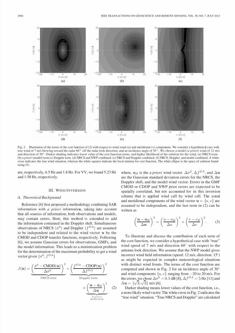
Fig. 2. Illustration of the terms of the cost function of (2) with respect to wind zonal (u) and meridional (v) components. We consider a hypothetical case withtrue wind of 7 m/s blowing toward the radar 60◦ off the radar look direction, and an incidence angle of 30◦. We choose a model (a priori) wind of 12 m/sand direction of 30◦. Darker shading indicates lower value of the cost function terms, and higher likelihood of the solution for the wind, (a) NRCS term.(b) a priori (model) term (c) Doppler term. (d) NRCS and NWP combined. (e) NRCS and Doppler combined. (f) NRCS, Doppler, and model combined. A whitecross indicates the true wind situation, whereas the white squares indicate the local minima for cost function. The white ellipse is the space of solution foundusing (5).

are, respectively, 6.5 Hz and 1.8 Hz. For VV, we found 5.23 Hz

and 1.58 Hz, respectively.

III. WIN D I NVERSION

A. Theoretical Background

Reference [6] first proposed a methodology combining SAR

information with a priori information, taking into account

that all sources of information, both observations and models,

may contain errors. Here, this method is extended to add

the information contained in the Doppler shift. Simultaneous

observations of NRCS (σ0) and Doppler (f DA) are assumed

to be independent and related to the wind vector u by theCMOD and CDOP transfer functions, respectively. Following

[6], we assume Gaussian errors for observations, GMFs, and

the model information. This leads to a minimization problem

for the determination of the maximum probability to get a wind

vector given {σ0, f DA}

J (u) =

σ0 − CMOD(u)

∆σ0

2

NRCS term

+

f DA − CDOP(u)

∆f DA

2

Doppler term

+u− uB

∆u

2

A priori

model term

(2)

where, uB is the a priori wind vector. ∆σ0, ∆f DA, and ∆u

are the Gaussian standard deviation errors for the NRCS, the

Doppler shift, and the model wind vector. Errors in the GMF

CMOD or CDOP and NWP prior errors are expected to be

spatially correlated, but not accounted for in this inversion

scheme that is applied wind cell by wind cell. The zonal

and meridional components of the wind vector u = {u, v} are

assumed to be independent, and the last term in (2) can be

written as

u− uB

∆u

2

=

u − uB

∆u

2

+

v − vB

∆v

2

. (3)

To illustrate and discuss the contribution of each term of

the cost function, we consider a hypothetical case with “true”

wind speed of 7 m/s and direction 60◦ with respect to the

antenna look direction. We assume that the NWP model gives

incorrect wind field information (speed: 12 m/s, direction: 15◦)

as might be expected in complex meteorological situations

with distinct wind fronts. The terms of the cost function are

computed and shown in Fig. 2 for an incidence angle of 30◦

and wind components {u, v} ranging from −20 to 20 m/s. For

the errors, we chose ∆σ0 = 0.5 dB [8], ∆f DA = 5 Hz [11] and

∆u = {√ 3;√

3} m/s [6].

Darker shading means lower values of the cost function, i.e.,

a more likely wind vector. The white cross in Fig. 2 indicates the“true wind” situation. “True NRCS and Doppler” are calculated




using CMOD and CDOP, respectively. The white squares indi-

cate the result obtained after minimization of the cost function.

Fig. 2(a)–(c) illustrates the contribution to the cost function

from the NRCS, model, and Doppler terms, respectively. When

only the NRCS is used to compute the cost function, there are

several minima (elliptic shape) corresponding to an undercon-

strained problem. The addition of the model term [Fig. 2(b)and (d)] accounts for both wind speed and direction and their

associated errors. When the a priori information departs too

much from the real wind situation, the Bayesian approach

cannot compensate the error. As shown in Fig. 2(c), the use

of Doppler shift alone would also lead to an underconstrained

problem. On the other hand, as shown in Fig. 2(e), the NRCS

and Doppler cost functions have distinct different shapes which

complement each other. In this case, the number of possible

solutions is dramatically reduced. Yet, ambiguities remain, and

a priori information is still needed in our inversion scheme

when a unique solution is required. The total cost function [(2)]

is shown on Fig. 2(f). All in all, the comparison of results with

[Fig. 2(d)] and without [Fig. 2(d)] the Doppler term in the cost

function illustrates how the Doppler shift helps to get better

winds.

As noticed by [18], the minimization can be reformulated if

the NRCS is assumed free of noise and if an inverse GMF is

used to relate radar configuration, NRCS, and wind direction

(with respect to the antenna look angle) to the wind speed

u10 = GMF−1(θ , φ, σ0, pol)φ∈[0,360◦]

. (4)

This inverse GMF enables to determine the possible solutions

{u10, φ} (or {u, v}) for a given radar configuration and NRCS.

Thus, combining (2) and (4), the cost function becomes

J (u) =

f DA − CDOP(u)

∆f DA

2

+

u− uB

∆u

2{u10=GMF−1(θ,φ,σ0,pol),φ}

. (5)

The space of solutions obtained with (4) in the context of the

previous simulation exercise is presented by the white ellipse

on Fig. 2.

Such kind of minimization performed wind cell by wind cell

in the SAR image is a local inversion. It does not take account

of spatially correlated errors, e.g., sea state errors in the GMF

and NWP prior errors are expected to be spatially correlated,

but not accounted for.

B. Application and Validation

We have selected two cases of complex meteorological sit-

uations to illustrate the wind signature of the Doppler shift,

and the performance of the method outlined in Section III. The

NRCS and the Doppler shift in VV polarization from Envisat

ASAR are shown in Fig. 3 together with ASCAT scatterometer

winds for a case with an atmospheric front (upper panels) and

for a low pressure system (lower panels). The NRCS winddependency is more driven by the wind speed than the direction,

whereas strong gradients of NRCS are generally associated

with rapid changes of the wind direction on short spatial scales.

Concerning the Doppler shift, in agreement with Section II,

there is expectedly a strong dependency on the wind direction

relative to the antenna look direction. For wind blowing along

the azimuth direction, the Doppler signal due to wind vanishes

and becomes positive (negative) for wind blowing toward (awayfrom) the radar. In addition, for a given direction, the Doppler

shift increases with wind speed. For an easier geophysical

interpretation, the Doppler shifts are converted to surface radial

velocity by the relation

V rad = −λ0f DA

2sin θ

where λ0 is the radar wavelength and θ is the incidence angle.

In the case of the atmospheric front [Fig. 3(a)–(c)],

ASCAT indicates that north of the front, the wind blows from

north—northeast and turns abruptly to become north-westerly

oriented. Comparing with ASAR NRCS, it can be observed

that no matter the wind direction, the NRCS increases with

increasing wind speed. Near the front, strong ASAR NRCS

gradients, ASCAT wind direction changes and radial velocities

sign switches are correlated. Thus, the combination of NRCS

and Doppler, can give a qualitative indication about the wind

field structure for a given scene.

In the case of the low pressure system [Fig. 3(d)–(f)], ASCAT

wind exhibits a clear circular pattern of the wind due to the low

pressure system. The changes of sign for the radial velocities

are consistent with this circular pattern. The sign is positive

south of the low pressure center where the circulation of the

flow is easterly, and negative to the north, where the flow iswesterly. The radial velocities are also in very good agreement

with ASCAT wind field.

For both these cases, we compared three different schemes:

1) scatterometry approach where wind is calculated with the

CMOD function [12] and the wind direction is given by a

model; 2) the Bayesian scheme where only NRCS and model

information are used; and 3) the Bayesian scheme combin-

ing Doppler, NRCS and model. Results by using the cost

function of (5) are presented in Fig. 4. Comparison with the

ASCAT wind fields clearly demonstrates the benefit of using

the Doppler with NRCS for wind inversion. When the Doppler

shift is included, the wind pattern as obtained with ASARcompares very well with ASCAT results. For the low pressure

system, the circular wind pattern is well captured by SAR

when Doppler is used [see Fig. 4(f)]. For the case with the

atmospheric front, when Doppler is used, the location of the

abrupt shift of wind direction is located where there is a strong

gradient of NRCS, in agreement with the ASCAT wind [see

Fig. 3(c)].

For a quantitative validation, we have colocated 103 SAR

images with wind measured by NDBC buoy number 42056

in the Caribbean Sea without any particular selection of me-

teorological situations. These cases do not correspond to any

particular complex meteorological situations, and the model is

not expected to be dramatically wrong. The statistics of theresults obtained using the Bayesian scheme with and without




Fig. 3. Two examples of wind signatures in the NRCS (left) and Doppler velocity signal (center) as measured by ASAR and corresponding wind field retrievedwith ASCAT (right). The upper panels show a case with an atmospheric front on 11 June 2010 at 21:27:32 UTC, and the lower panels show a case with a lowpressure system on 12 August 2008 at 21:20:58 UTC. The sign convention for the radial velocity is such that when radial velocity is positive (respectively negative)wind is blowing from the west (respectively east).

the Doppler are shown in Table I. The wind direction is much

more accurate for the scheme including the Doppler shift, with a

RMS of 14◦, compared to 30◦ for the same scheme without the

Doppler information. This improvement in the wind direction

RMS is due to the few cases where the a priori information and

the in situ measurement are strongly inconsistent. For the wind

speed, we find in fact a slightly decreased performance when

Doppler shift is included. It is likely due to the high uncertainty

of the Doppler centroid anomaly, as it is still to be considered as

an experimental derived quantity in the Envisat ASAR ground

segment. In particular, when the a priori wind information and

the NRCS are very consistent, the use of Doppler anomaly

can add noise to lower the performance the inversion scheme

(Table II).

IV. CONCLUSION

Hitherto the investigations of the Doppler shift signals have

mostly been conducted in areas with strong surface currents,

such as in the Agulhas Current, to derive and analyze estimatesof the surface current [9]. However, as demonstrated by [7]

the Doppler shift anomaly results from a mixture of sea state

displacements from the wind, waves, and currents.

This study shows that the Doppler anomaly as measured

by SAR at C-band is indeed wind dependent with respect

to polarization, incidence angle, and antenna look direction.

This dependency is found to be complementary to the NRCS.

Using a Bayesian scheme, we demonstrate how these two

radar quantities, i.e., NRCS and Doppler anomaly, could be

advantageously used to increase the weight of the SAR data in

the SAR wind inversion schemes. In particular, it is found that

the high sensitivity of the Doppler to the wind direction is useful

to retrieve more realistic wind patterns in cases of complex and

rapidly changing meteorological situations. Thus, for coastal

wind regimes and extreme events such as hurricanes, typhoons,

and polar lows where the SAR images may be colocated with

incorrect a priori wind field information (particularly the wind

direction) the incorporation of the Doppler shift will provide

highly valuable information.

Today, the Doppler shift is not provided as a geophysical

product and is not routinely used for geophysical inversion by

the scientific community. Accordingly, the precision require-ments, which are a few Hertz for sea surface current estimation




Fig. 4. (Top panel) Case of an atmospheric front on 11 June 2010 at 21:27:32 UTC. (a) Scatterometry approach, where the wind direction is given by the a priori

information. (b) Bayesian scheme without Doppler shift, (c) Bayesian scheme including Doppler. (Bottom panel) The same for the case of a low pressure systemon 11 June 2010 at 21:27:32 UTC.

TABLE I

STATISTIC OF VALIDATION E XERCISE PERFORMED

AGAINST I N -S ITU MEASUREMENTS

or wind estimation, are not yet achieved. Additional correction

steps must thus be performed. In particular, antenna characteris-

tics have to be more accurately known. Yet, the results found in

this study are very encouraging. In particular, for future SAR

missions such as Sentinel-1, the Doppler anomaly will be a

standard component of the L2 ocean product. The method will

then benefit of more accurate Doppler anomalies and a new

improved version of CDOP could be developed. In the future,

the Bayesian scheme could further be improved by using a

nonlocal inversion scheme and a better description of the errorstructures.

New more accurate radar quantities are then foreseen to

provide improved information for both wind field and surface

current inversions. Ideally, next refined step could thus be

a more consistent synergetic approach where the NRCS and

the Doppler shift information would be combined to derive

improved estimates of both the near surface wind field and

the sea surface currents (using a priori routine atmosphere and

ocean circulation model first guess). A complementary Doppler

and NRCS capability may be interesting for future scatterom-

eter systems. Indeed, the multi-azimuth angular dependenceassociated with NRCS and Doppler measurements would then

allow better constraining the inversion problems.

APPENDIX

Doppler shift due to sea surface wind can be written as

∆f pp = α ppF [X (θ , φ, u10, pp)] + β pp

where θ is the incidence angle in degree, φ the wind direction

with respect to the antenna look angle in degrees (where 0

(respectively, 180◦) means wind blows toward (respectively,

against) the antenna. Thus, 90◦ and 270◦ mean wind blow indirection perpendicular to the antenna look direction.), u10 the




TABLE IISET OF ωi,j C OEFFICIENTS FOR HH A ND VV POLARIZATIONS

wind speed and pp denotes the polarization. α pp and β pp are

two coefficients depending on polarization

αvv =111.528184073 and β vv = −52.2644487109

αhh =136.216953823 and β hh = −

66.9554922921

and F [x] is defined as

F (x) = 1

1 + e−x

X (θ , φ, u10, pp) = γ pp0 +

11i=1

γ ppi F

Γ ppi (θ, φ̃, u10)

where

Γ ppi (θ, φ̃, u10) = ω ppi,0 + ω

ppi,1V 1(φ̃) + ω

ppi,2V 3(u10) + ω

ppi,3V 2(θ)

V pp = V pp1

V pp2

V pp3

= φ̃

·λ pp20 + λ

pp21

θ · λ pp00 + λ pp01

u10 ·λ pp10 + λ

pp11

φ̃ =

360◦ −φ, if φ < 180◦

φ, otherwise.

The set of coefficients ω for each polarization is given in

Table II.

ACKNOWLEDGMENT

The authors would like to thank the European Space Agency

(ESA) and in particular Betlem Rosich that helped modify

ENVISAT ASAR Wide swath products to include Dopplercentroid grids. This work was supported by ESA under

wind/wave/current study contract and ccn, by the French Ma-

rine Hydrographic and Oceanographic center (SHOM) under

contract 05.87.028.00.470.29.25 contract and the European

Commission through NORSEWIND contract.

REFERENCES

[1] F. M. Monaldo and V. Kerbaol, “The SAR measurement of ocean surfacewids: An overview,” in Proc. 2nd Workshop Coastal Marine Appl. SAR,8–12 September 2003, Svalbard, Norway, Jun. 2004, ESA SP-565.

[2] A. Stoffelen and D. Anderson, “Scatterometer data interpretation: Estima-tion and validation of the transfer function CMOD4,” J. Geophys. Res.,vol. 102, no. C3, pp. 5767–5780, 1997.

[3] F. M. Monaldo, D. R. Thompson, W. G. Pichel, and P. Clemente-Colon,“A systematic comparison of QuikSCAT and SAR ocean surface windspeeds,” IEEE Trans. Geosci. Remote Sens., vol. 42, no. 2, pp. 283–291,Feb. 2004.

[4] W. Koch, “Directional analysis of SAR images aiming at wind direc-tion,” IEEE Trans. Geosci. Remote Sens., vol. 42, no. 4, pp. 702–710,Apr. 2004.

[5] C. C. Wackerman, C. L. Rufenach, R. A. Shuchman, J. A. Johannessen,

and K. L. Davidson, “Wind vector retrieval using ERS-1 synthetic aper-ture radar imagery,” IEEE Trans. Geosci. Remote Sens., vol. 34, no. 6,pp. 1343–1352, Nov. 1996.

[6] M. Portabella, A. Stoffelen, and J. A. Johannessen, “Toward an optimalinversion method for SAR wind retrieval,” J. Geophys. Res., vol. 107,p. 8, 2002, doi:10.1029/2001JC000925.

[7] B. Chapron, F. Collard, and F. Ardhuin, “Direct measurements of oceansurface velocity from space: Interpretation and validation,” J. Geophys.

Res., vol. 110, p. C07008, Jul. 2005.[8] ASAR Product Handbook , 2007, issue 2.2.[9] J. A. Johannessen, B. Chapron, F. Collard, V. Kudryavtsev, A. Mouche,

D. Akimov, and K.-F. Dagestad, “Direct ocean surface velocity mea-surements from space: Improved quantitative interpretation of EnvisatASAR observations,” Geophys. Res. Lett., vol. 35, p. L22608, Nov. 2008,doi:10.1029/2008GL035709.

[10] M. J. Rouault, A. Mouche, F. Collard, J. A. Johannessen, and B.

Chapron, “Mapping the Agulhas current from space: An assessment of ASAR surface current velocities,” J. Geophys. Res., vol. 115, p. C10026,Oct. 2010, doi:10.1029/2009JC006050.




[11] M. W. Hansen, F. Collard, K. Dagestad, J. A. Johannessen, P. Fabry, andB. Chapron, “Retrieval of sea surface range velocities from Envisat ASARDoppler centroid measurements,” IEEE Trans. Geosci. Remote Sens.,vol. 49, no. 10, pp. 3582–3592, 2011, doi:10.1109/TGRS.2011.2153864.

[12] Y. Quilfen, B. Chapron, T. Elfouhaily, K. Katsaros, and J. Tournadre,“Observation of tropical cyclones by high-resolution scatterometry,”

J. Geophys. Res., vol. 103, no. C4, pp. 7767–7786, 1998, doi:10.1029/ 97JC01911.

[13] H. Hersbach, A. Stoffelen, and S. de Haan, “An improved C-band scat-terometer ocean geophysical model function: CMOD5,” J. Geophys. Res.,vol. 112, p. C03006, Mar. 2007, doi:10.1029/2006JC003743.

[14] A. Mouche, B. Chapron, N. Reul, and F. Collard, “Predicted Dopplershifts induced by ocean surface displacements using asymptotic elec-tromagnetic wave scattering theories,” Waves Random Complex Media,vol. 18, no. 1, pp. 185–196, Feb. 2008.

[15] B. Chapron, V. Kerbaol, and D. Vandemark, “A note on relationshipbetween sea-surface roughness and microwave polarimetric backscat-ter measurements: Results from POLRA-96,” in Proc. POLRAD’96 Int.

ESA Workshop, ESA WPP-135, ESTEC , Noordwijk, The Netherlands,Apr. 29, 1997.

[16] ASCAT 12.5 km Wind Product User Manual v 1.8, OSI-SAF Project Team,2010.

[17] F. Collard, A. Mouche, B. Chapron, C. Danilo, and J. Johannessen, “Rou-tine high resolution observation of selected major surface currents fromspace,” in Proc. SEASAR Symp., SP-656, ESA, ESA-ESRIN , Frascati,

Italy, 2008.[18] V. Kerbaol, “Improved Bayesian wind vector retrieval scheme using

ENVISAT ASAR data: Principles and validation results,” in Proc. ENVISAT Symp., Montreux, Switzerland, Apr. 23–27, 2007.

Alexis A. Mouche received the Master degree inphysics for remote sensing from the University of Pierre et Marie Curie, Paris, France, in 2002. From2002 to 2005, he worked as a Ph.D. student atCETP/IPSL/CNRS (National Research Center) andreceived the Ph.D. degree in physics with a focus onocean remote sensing in 2005.

Since January 2006, he has been working onapproximate scattering wave theories from random

ocean surface in the Spatial Oceanography group atIFREMER, Brest, France. This postdoctoral positionwas Granted by CNES (French Space Agency). He joined BOOST Technolo-gies in 2008 and works now in the R&D Department at the Radar ApplicationsDivision of CLS, Plouzané, France.

Fabrice Collard received the M.S. degree from theEcole Centrale de Lyon, Ecully, France, in 1996,where he studied off-shore engineering and thePh.D. degree in oceanography and meteorology fromParis 6 University, Paris, France, in 2000.

Histhesis wasdedicated to the3-D aspectof wind-wave field. He spent two years working on HF radarsas a postdoctoral research associate at RSMAS,Miami. He is currently Head of the R&D Depart-

ment at the Radar Applications Division of CLS,Plouzané, France, working on the development andvalidation of surface wind, wave, and current retrieval from synthetic apertureradar.

Bertrand Chapron was born in Paris, France, in1962. He received the B.Eng. degree from the Insti-tut National Polytechnique de Grenoble, Grenoble,France, in 1984 and the Doctorat National (Ph.D.)degree in fluid mechanics from the University of Aix-Marseille II, Marseille, France, in 1988.

He spent three years as a Post-Doctoral Re-search Associate at the NASA/GSFC/Wallops FlightFacility, Wallops Island, VA. He has experiencein applied mathematics, physical oceanography,

electromagnetic waves theory, and its application toocean remote sensing. He is currently responsible for the Oceanography fromSpace Laboratory, IFREMER, Plouzané, France.

Knut-Frode Dagestad received the Cand. Scient.and Dr. Scient. degrees from University of Bergen,Bergen, Norway, in 2000 and 2005, respectively.

The thesis work was performed at the Geophys-ical Institute, in the field of atmospheric radiativetransfer with application to solar energy. Since 2005,he has been working with remote sensing at theNansen Environmental and Remote Sensing Center,

Bergen. The main research interest is retrieval of wind, waves, and currents from remote sensing data,with focus on synthetic aperture radar.

Gilles Guitton received the M.Sc. degree fromENST-Bretagne, Brest, France, in 2007, within spa-tial oceanography and ocean monitoring, where heis currently working toward the Ph.D. degree onhurricanes.

During his M.Sc. degree study, he visited Norut,Tromsø, Norway, from April 2006 to October 2006,as a Trainee, where he worked with an EM scatteringmodel for the ocean surface.

Johnny A. Johannessen received the Dr. Philos. de-gree from the University of Bergen, Bergen, Norway,in 1997.

He is Vice Director at the Nansen Environmentaland Remote Sensing Center, Bergen. His experiencein satellite remote sensing in oceanography and seaice research is broad and comprehensive. In particu-lar, he has focused on the use of synthetic apertureradarimaging capabilities to advance the understand-ing of mesoscale processes along the marginal icezone and in vicinity of ocean fronts and eddies. In

the last 10 years, he has also been involved in development and implementationof operational oceanography and marine forecasting both at national andinternational level.

Vincent Kerbaol graduated from the Ecole Na-tionale Supérieure des Télécommunications deBretagne, Bretagne, France, in 1992 with emphasisin image processing. He received the Ph.D. degree insignal/image processing and remote sensing from theUniversity of Rennes 1, Rennes, France, in 1997.

He is Head of the Radar Applications Divisionsat CLS, Plouzané, France. After doing his civil ser-vice in Tromsoe, Norway, he worked as a Ph.D.student on ocean synthetic aperture radar (SAR) Im-ages at the Oceanography from Space laboratory at

IFREMER, Brest France. He stayed at IFREMER up to February 1999, as apostdoc Granted by CNES (French spaceagency), mainly working on altimetry.In March 1999, He joined the ENST Bretagne in the Départment Signal and

Communications as an Assistant Professor. His works mainly include sea stateretrieval, from SAR imagery and altimetry, radar technology, and signal/imageprocessing.

Morten Wergeland Hansen received the Cand. Sci-ent. degree in astrophysics from the University of Oslo, Oslo, Norway, in 2004, with a thesis on theorbits of Jupiter’s Galilean satellites and the M.Sc.degree in space studies from the International SpaceUniversity, Strasbourg, France, in 2006, with a thesison the validation of level-2 products from the atmo-spheric instruments aboard Envisat.

He has been with the Nansen Environmental andRemote Sensing Center, Bergen, Norway, since 2007

as a Research Assistant and later as a Ph.D. candidatewith focus on the development and utilization of the Doppler velocity productfrom Envisat ASAR.

Documents

Doppler Shift