Embed Size (px)
Citation preview

1
Does the Model Matter? A Valuation Analysis
of Employee Stock Options
Manuel Ammann and Ralf Seiz1
This version: March 2004
Abstract
We present a numerical analysis of valuation models for employee stock options. In
particular, we analyze the impact of the model on the resulting option prices and
investigate the sensitivity of pricing differences between models with respect to changes in
the parameters. We show that, for most models such as the FASB 123 model, the utility-
maximizing model by Rubinstein, the Hull-White model, and a simple reference model
proposed in this paper, the price reduction relative to standard options is uniquely
determined by the expected life of the option. In fact, with the exception of the FASB 123
model, pricing differences are negligible if the models are calibrated to the same expected
life of the option. Consequently, the application of models with several hard-to-estimate
parameters such as the utility-maximizing model can be greatly simplified by this
calibration approach because expected life is easier to estimate than utility parameters.
1 Manuel Ammann is professor of finance and Ralf Seiz is research assistant at the University of St. Gallen. Address: Swiss Institute of Banking and Finance, University of St. Gallen, Rosenbergstrasse 52, 9000 St.Gallen, Switzerland. Tel: +4171-224-7090, Fax +4171-224-7088, Email: [email protected], [email protected].

2
1 Introduction
Employee stock options present a number of specific issues that prevent their valuation
with standard option pricing models. Although several pricing models for employee stock
options have been proposed, no standard model has been established to this date. As a
contribution to the ongoing model discussion, we present a detailed side-by-side
comparison of option prices obtained with several models. In particular, we investigate a
utility-maximizing model as proposed by Kulatilaka and Marcus (1994), Huddart (1994)
and Rubinstein (1995), a recent model by Hull and White (2002, 2004), and the model
proposed by the Financial Accounting Standards Board (1995), referred to as FASB 123.
Furthermore, we propose a new model that accounts for sub-optimal exercise because of
non-tradability by a simple adjustment of the exercise price. This model is called Enhanced
American because of its similarity with a standard American option. In addition, all these
models are also compared to standard Black-Scholes and American-style options.
We show that, with the exception of the FASB 123 model and the standard Black-Scholes
and American models, these models produce virtually identical option prices (differences
in the range of -0.4% and +0.4%) if they are calibrated to the same expected life. In fact,
for most models accounting for premature exercise of the option, expected life is a
sufficient parameter to determine the price of an employee stock option relative to a
standard option. In other words, even though the models tested derive their exercise
policies using completely different approaches, the pricing effect of the different exercise
schemes is negligible as long as the expected life of the option is the same.
3
As a consequence, the drawback of the dependence on unobservable and hard-to-estimate
parameters, such as the risk aversion coefficient in the utility-maximizing model, can be
overcome by using the expected life, which is much easier to estimate, to calibrate the
model. Expected life can replace the utility parameters because, as shown below, any
combination of utility parameters implying the same expected life for the option produces
the same option price.
In the following section, the modeling methodology is described in general. In Section 3,
the specific models investigated are outlined and a new model is proposed as a simple
reference. Section 4 compares the prices derived by different models and Section 5 adds a
sensitivity analysis to the comparison. In Section 6, we extend the existing models by
allowing a variable employee exit rate depending on the moneyness of the option during
the vesting period. Section 7 concludes.
2 General Setup of Pricing Models for Employee Stock Options
The models for valuing employee stock options discussed in this paper are implemented
with a generalized binomial-tree method. For the binomial-tree method, we use the
standard specifications as originally proposed by Cox, Ross, and Rubinstein (1979). A
technical description of the general binomial-tree framework used in this paper is included
in Appendix A.

4
Employee stock options (ESO) differ from standard exchange-traded options in important
aspects (see, for example, Rubinstein 1995) and several researchers have noted the
shortcomings of using traditional option formulas to value employee stock options2. In the
following, we identify the three main differences and explain how they can be
implemented in a valuation model for employee stock options:
A. Vesting Period: Employee stock options can only be exercised after the vesting period
v. Delayed vesting can be handled easily by modifying the standard binomial model such
that exercise is not allowed during the vesting period.
B. Exit Rate: Employees lose unvested employee stock options if they leave voluntarily or
involuntarily during the vesting period and may be forced to exercise unexercised but
vested options prematurely upon leaving the firm. Thus, employee stock options are
exercised earlier than optimally exercised standard American options. The probability of
employees leaving the firm is modeled by the exit rate3 w and given for each period of time
∆t as (1 − ∆− w te ). In a first step we assume that the exit rate w (pre- and post-vesting) is
constant over time. In a second step, in Section 6, we implement an extended model that
incorporates a (pre-vesting) exit rate contingent on the moneyness of the option.
If an employee leaves during the vesting period v, employee stock options are forfeited and
the exit value of the option equals 0. If the employee leaves after the vesting period v, the
option is forfeited if it is out of the money and exercised (immediately) if it is in the
2 See especially Lambert, Larcker, and Verrecchia (1991), Smith and Zimmerman (1976), Kulatilaka and Marcus (1994), Rubinstein (1995), Carpenter (1998), DeTemple and Sundaresan (1999), Hall and Murphy (2000, 2002).
5
money. On the other hand, if the employee does not leave during the vesting period, the
value of the option equals the holding value using risk-neutral valuation. Furthermore, if
the employee does not leave after the vesting period, there are two possibilities: either the
option will be exercised or held.
Appendix A describes the setup of the binomial model for standard American options
adjusted for the exit rate and the vesting period. We refer to the binomial model for
standard American options as AM-model and the binomial model adjusted for the exit rate
and the vesting period as described in Appendix A as AM Ex&Vest-model.
C. Non-Transferability: Employees are not allowed to sell their employee stock options.
Because of this non-transferability, an earlier exercise is often the only way of raising cash
from the option. Several researchers have documented that employee stock options are
exercised relatively early in their term, even when the underlying stock pays no dividends
(see, for example, Huddart and Lang 1996). Such sub-optimal exercise reduces the
option’s value. The time when a particular employee exercises the option may depend on
several factors such as risk-aversion, liquidity requirements, diversification motives, non-
option-wealth, expected stock-return, utility function, underlying stock price, etc. Thus, an
individual exercise scheme will be determined that characterizes an employee or a group of
employees with similar exercising behavior. Therefore, for a group of employees of a
certain exercise type, the expected life of the option can be estimated with reasonably
accuracy. For calculating the expected life we use the conditional procedure described by
3 We refer to the continuous exit rate as w and to the annually compounded exit rate as wa.c.
6
Hull and White (2002), which is an expectation conditional on the option vesting.
Appendix B describes the calculation of the risk-neutral expected life in the binomial tree.
The expected life of a set of employee stock options is defined as the length of time that
options remain unexercised on average given that they vest. We choose this definition for
empirical convenience because only options that have vested need to be considered for
empirical estimation of expected life. Note that, using this definition, the expected life of
the option is always smaller than the maturity because the exit rate is greater than zero after
the vesting period. Of course, several alternative definitions of expected life are possible,
such as expected life conditional on no exit or on exercise of the option. However, the
contributions of this paper are not dependent on the definition of expected life.4
The expected life is not invariant to the probability measure. Our definition of expected life
is a risk-neutral expected life. In risk-averse economies, employee stock options are
exercised sooner than in risk-tolerant economies (see Garman 1989). The results in this
paper, however, are unaffected by this issue because we use the same definition of
expected life for all models.5
4 We also calculated the option prices presented in Sections 4 and 5 using different definitions of expected life. Because the results are very similar and do not add any new insights, they are not presented. 5 See Section 4.2.

7
3 Employee Stock Option Pricing Models
3.1 The FASB 123 model
The Financial Accounting Standards Board (1995) announced a proposal, denoted FASB
123, for a valuation model for employee stock options. In that document, both the Black-
Scholes model and the binomial tree model are deemed acceptable. FASB 123 proposes to
set the maturity of the option equal to the expected life (L). This is the average time the
option stays in existence assuming the employee does not leave during the vesting period.
Thus, FASB 123 accounts for the non-transferability after the vesting period by
substituting6 the options’ contractual life (T) for their expected life (L) (i.e., T=L).
FASB 123 makes another adjustment to reflect that the employee stock option might be
forfeited during the vesting period because the employee leaves, i.e.,
123 ,. .(1 )FASB AM L T v
a cf f w== ⋅ − (3.1)
where 123FASBf denotes the value of the option using the FASB 123 method, AMf the value
of an American-style option using the binomial-tree framework, wa.c the annually
compounded exit rate, and v the duration of the vesting period. Although FASB 123 allows
also the Black-Scholes model, the binomial-tree method used in this paper (AM-model)
6 FASB exposure draft recognizes the potential for early exercise. However, the procedure accounting for an employee’s propensity to exercise the option early is overly simplistic. This model drawback is described in Kulatilaka and Marcus (1994), Hemmer and Matsunaga (1994), and Rubinstein (1995).

8
seems more appropriate because employee stock options can generally be exercised prior
to maturity.
3.2 The Utility Maximization Model
3.2.1 Setup of the model
The utility maximization model7 (UM-model) assumes that employees do not maximize
the expected value of the option but rather their utility. Kulatilaka and Marcus (1994) and
Rubinstein (1995) propose the following utility function U,
1
( ) ; ( ) ln if 11
−γ
= = γ =− γ
WU W U W W (3.2)
where W is the total wealth of an employee consisting of non-option wealth8 W0 and wealth
in the form of employee stock options. The model assumes that both non-option wealth
and cash realized from exercising the options are reinvested in risk-free assets. γ is the
coefficient of the employee’s risk aversion. At the end of the binomial tree, at time T, the
option is either exercised or forfeited. Thus, in the end nodes (i=N) we have the following
utility function,
, 0 ,[ max( ,0)]= ⋅ + −rTN j N jU U W e S X . (3.3)

9
where ,N jS denotes the stock prices in the end nodes, X the strike price of the option, and
W0 the initial non-option wealth of the employee.
By working back through the tree from the end to the beginning of the life of the option,
we have to keep in mind that employees base their exercise decisions on their own
subjective expectation about the expected stock return µ and not on risk-neutral
expectations. Consequently, for the probability of an up-movement
( )( ) /( )µ− ⋅∆π = − −D te d u d , the risk-free rate r is replaced by the subjective expected stock
return µ , where ∆t denotes the time step in the binomial tree, D the continuous expected
dividend yield, u and d the up- and down-movement factors of the stock price.
The rules for calculating the utility in each node of the binomial tree are described in
Appendix C. The option is exercised after the vesting period if the expected utility derived
from holding the option (conditional expectation using probabilities π ) is smaller than the
utility from exercising (this is the utility of the non-option wealth plus the cash realized
from exercising the option, both invested in risk-free assets). This utility tree determines
the individual exercise scheme of the employee. Using this exercise scheme and working
backward through the tree, the value of the option can be determined.
7 See Kulatilaka and Marcus (1994), Huddart (1994) and Rubinstein (1995). 8 The non-option wealth must be adapted to the number of options held.
10
3.2.2 Calibrating the UM-Model
An apparent drawback of the UM-model is its dependence on a specific utility function and
the need for estimation of three parameters µ (expected return), W0 (non-option wealth) and
γ (risk aversion). Whereas non-option wealth can be observed for individual employees,
the expected return on the stock and the risk-aversion coefficient are unobservable and
notoriously hard to estimate.
However, it turns out that the specification of the utility function and the three parameters
imply an expected life of the option and that this expected life is sufficient for computing
the price of the option. Thus, if the expected life of the option is known or can be
estimated, the price of the option can be computed without estimating the three parameters.
Although unobservable, the expected life of the option is easier to estimate than the three
parameters because empirical data on exercise behavior exists for different groups of
employees.
To demonstrate the relationship between the original parameters of the UM-model, the
expected life of the option, and the value of the option, we compute the expected life as
well as the option price from a given set of example parameters. In particular, we show
that, for arbitrary parameter combinations, the same price results for the same expected
life. In other words, the price of the option can be written as a function of the expected life
only.

11
We define S as the initial stock price, X as the strike price of the option, σ as the volatility
of the underlying stock, r as the continuous risk-free rate, D as the continuous expected
dividend yield, T as the life of the option (time-to-expiration), wa.c. as the annually
compounded exit rate and v as the vesting period. For a given set of standard input
parameters9 (sample option with S = $50, X = $50, σ = 30%, r = 5%, D = 2.5%, T = 10
years, wa.c. = 6%, v = 3 years) we choose the risk aversion from the set [0, 1, 2, .., 9, 10],
the expected stock return from the set [5.0%, 5.5%, 6.0%, .., 9.5%, 10.0%] and the non-
option wealth from the set10 [$0, $20, $40, .., $180, $200]. All possible combinations of
these parameter sets give 1331 unique triples of parameter combinations, each
characterizing an employee. For each of the triples, the expected life and the price of the
option is computed.
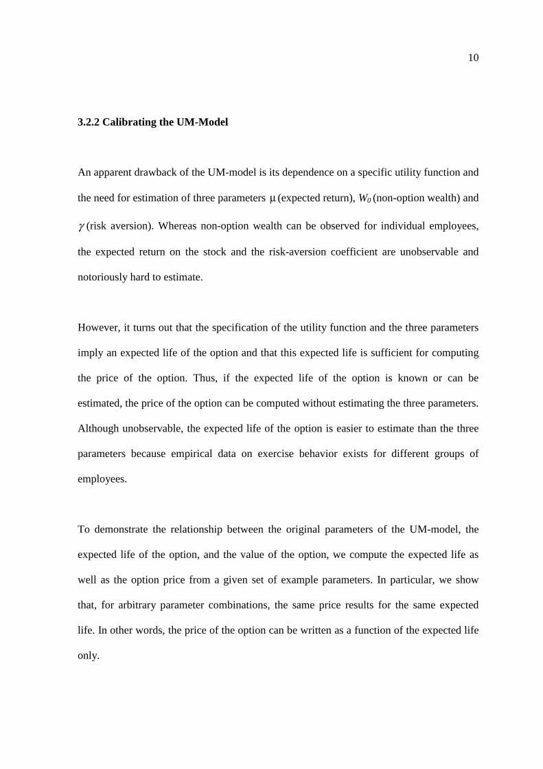
[Figure 1]
Figure 1 shows the price of the option in relation to the expected life for all 1331 parameter
combinations. It can be seen that the expected life of the option uniquely determines the
value of the option. It is possible to show that this is a general result valid also for other
input parameters and other option specifications.
Because arbitrary combinations of the three parameters risk aversion, expected stock
return, and non-option wealth determine a unique relation between the expected life and
the value of the option, the UM-model can be used without estimating those parameters.
9 The standard example (example option) used in this paper is similar to the example used by Hull and White (2002), but the risk-free rate is set to 5%. The parameters are annualized with r and D assumed to be continuously and wa.c annually compounded.
12
All that is needed is an estimation of the expected life of the option, from which the
parameter values can be inferred using a calibration procedure.
Figure 1 shows a maximum price at an expected life of 8.16 years and a value of the option
of $14.30. Because of the dividend yield, it is optimal to exercise the option before
maturity. For firms with dividend yields closer to the risk-free rate, this effect is more
pronounced because early exercise is even more desirable, thus reducing the expected life
of the option. Note that in Figure 1 the contractual life T cannot be reached because the
non-zero exit rate implies an expected life of less than the time to maturity of the option.
3.3 The Hull-White Model
Hull and White (2002, 2003, 2004) propose a model for valuing employee stock options
that they refer to as the Enhanced FASB 123 model. They model the early exercise
behavior of employees by assuming that exercise takes place whenever the stock price ,i jS
reaches a certain multiple M of the strike price X (i.e., ,i jS X M≥ ⋅ ) and the option has
vested. The Hull-White model (HW-model) is an extension of the binomial tree model.
Unlike the FASB 123-model described in Section 3.1, the HW-model explicitly considers
the possibility that the employee will leave the company after the vesting period and it
explicitly incorporates the employee’s early exercise policy. Appendix D gives the rules
for calculating the value of the option in the binomial-tree framework for the HW-model.
10 For technical reason we use $10-12 instead of $0.

13
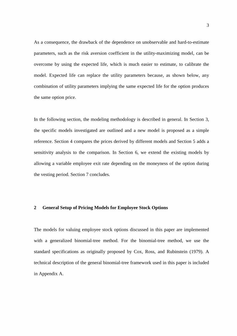
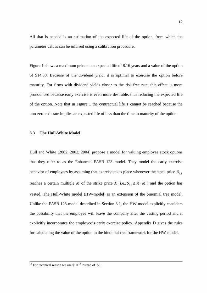
[Figure 2]
Figure 2 shows the relation between the multiple M that determines the exercise policy and
the value of the option. As we can see, there is a multiple M where the option has a
maximum price. However the value of the option for the HW-model is always below the
value using an American model adjusted for the exit rate and the vesting period
(see Section 2 and Appendix A for the AM Ex&Vest-model). Compared to the optimal
exercise strategy in the AM Ex&Vest-model, the HW-model always uses a sub-optimal
exercise strategy even at the maximum price attainable by the model due to the rigid
exercise scheme.
3.4 The Enhanced American model
In this section, we present a new model for valuing employee stock options. The model
belongs to the family of the UM- and HW-models as seen later. It considers a vesting
period, the possibility that employees may leave the company during the life of the option,
and non-transferability.
The general approach is similar to the American model adjusted for the exit rate and the
vesting period, but this model (called Enhanced American or EA-model) explicitly
incorporates the employee’s early exercise policy. This incorporation is simple: it consists
only of an adjustment of the strike price of the option. Of course, the adjusted strike price
is used only to determine the time of exercise, not to calculate the payoff of the option. The

14
adjustment factor is denoted by a multiple M* that triggers premature or late exercise
depending on its value.
We model the early exercise behavior of employees by assuming that exercise takes place
whenever there is a positive intrinsic value and the exercise value adjusted by the factor M*
is larger than the holding value11 (i.e., *, 1, 1 1,max( ,0) [ (1 ) ]r t
i j i j i jS M X e pf p f− ∆+ + +− ⋅ ≥ ⋅ + − )
and the option has vested. Appendix E describes the Enhanced American model in detail.
For a multiple of M*=1, the EA-model and American model (AM Ex&Vest) are the same.
For M* smaller and greater than 1, the EA model accelerates or delays exercise,
respectively, and thus allows for the individual, sub-optimal exercise policy similar to the
UM- and the HW-models.
The Enhanced American model shows that by making a very small adjustment to the
standard American-model (AM Ex&Vest, i.e., adjusted for the exit rate and the vesting
period), a model with all the features of the UM-model and the HW-model can be obtained
in a very simple way.
The multiple M* used in the Enhanced American model is similar to the one used in the
HW-model, because M* is also a multiple of the strike price X. However, in contrast to the
HW-model, M* multiplied by the strike price X represents a virtual strike price of a specific
employee. In the EA-model the employee decides to exercise the option if he is satisfied
with the intrinsic value relative to his virtual strike price M*X.

15
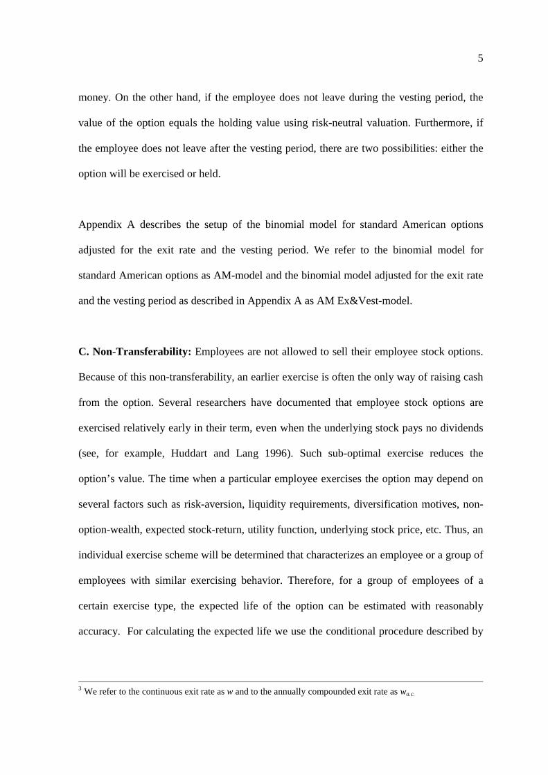
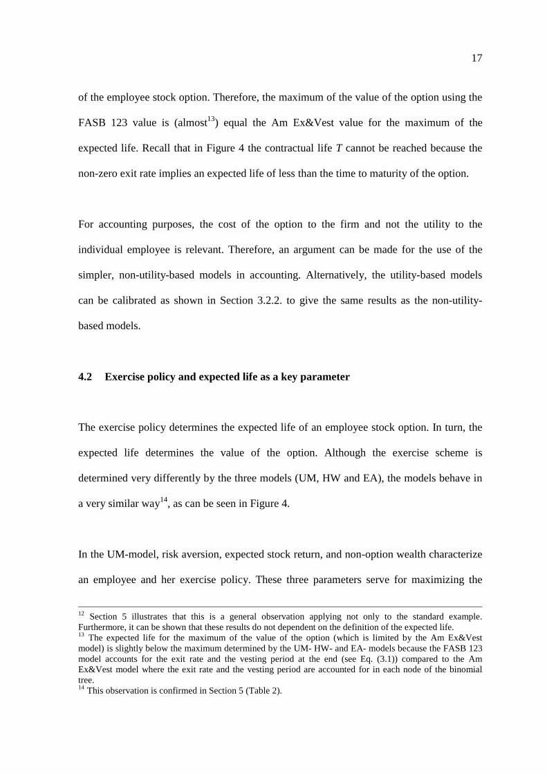
[Figure 3]
Figure 3 shows the relation between the multiple M*, which determines the exercise policy,
and the value of the option. As we can see, there exists a multiple M* where the value of
the option has a maximum price. In contrast to the HW-model, where the best achievable
exercise strategy is still sub-optimal, this maximum price implies an optimal exercise
policy and is therefore equal to the price obtained by the American-model adjusted for the
exit rate and the vesting period (AM Ex&Vest model).
4 Comparison of the Models
4.1 Two different types of models
Two types of models for employee stock options can be identified. The first type accounts
for the individual exercise policy (i.e., accounts for the non-transferability), the second
type does not. The FASB 123, UM, HW, and the EA models belong to the first type, the
Black-Scholes model, the standard American model, the adjusted American model (AM
Ex&Vest) belong to the second type where the exercise policy is assumed to be optimal
and therefore the same for all employees.
Furthermore, we have seen that for the first model type, the exercise policy and therefore
the expected life of an option can be determined differently. Note that in the UM-, HW-,
11 For a detailed variables description see Appendix A and Appendix E.

16
and EA-model the exercise policy is implemented more precisely than in the FASB 123-
model, where the life of the option is set to the expected life. In the UM-model, the
parameters risk aversion, expected stock return and non-option wealth trigger the exercise,
in the HW-model the multiple M and in the EA-model the multiple M*. These factors
determine therefore the expected life of the option.
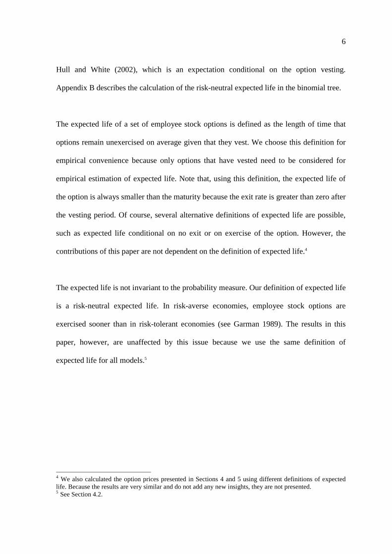
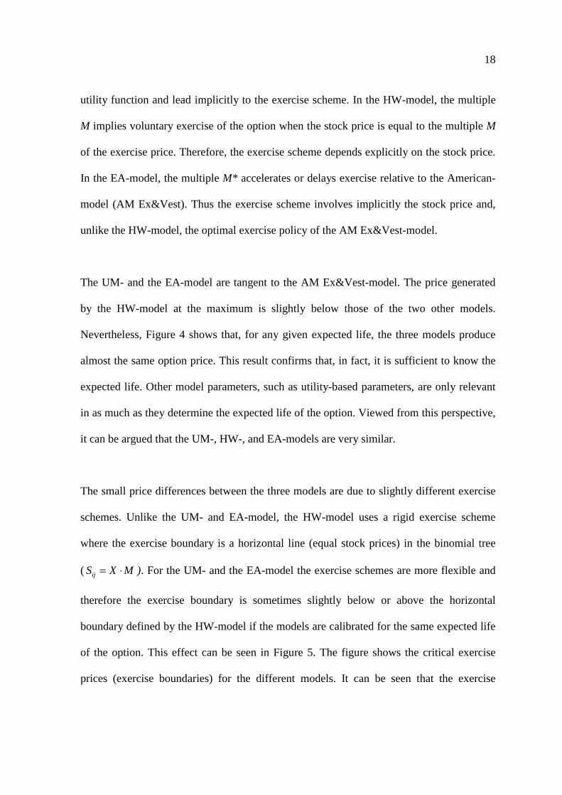
[Figure 4]
Figure 4 shows the value of an employee stock option depending on the expected life
calculated for a number of models. For models of the second type, the expected life
remains constant for all employees because there is only one exercise scheme possible.
This exercise scheme is optimal and determined by the input parameters S, X σ, r, D, T, w,
and v only. This applies to the standard American model (AM), the American model
adjusted for the vesting period only (AM Vest), the American model adjusted for the exit
rate only (AM Ex), the American model adjusted for the exit rate and the vesting period
(AM Ex&Vest) and the Black-Scholes model (B/S).
With the exception of the FASB 123 model, the models of the first type (UM-, HW- and
EA-model) show a very similar price behavior12. Figure 4 also indicates that expected life
is one of the driving factors for the value of an employee stock option (valued by models
allowing for individual exercise policies). In fact, the price can be expressed as a function
of the expected life of the option. Furthermore the maturity of T=10 years is not
incorporated in the FASB 123 model because the maturity is replaced by the expected life
17
of the employee stock option. Therefore, the maximum of the value of the option using the
FASB 123 value is (almost13) equal the Am Ex&Vest value for the maximum of the
expected life. Recall that in Figure 4 the contractual life T cannot be reached because the
non-zero exit rate implies an expected life of less than the time to maturity of the option.
For accounting purposes, the cost of the option to the firm and not the utility to the
individual employee is relevant. Therefore, an argument can be made for the use of the
simpler, non-utility-based models in accounting. Alternatively, the utility-based models
can be calibrated as shown in Section 3.2.2. to give the same results as the non-utility-
based models.
4.2 Exercise policy and expected life as a key parameter
The exercise policy determines the expected life of an employee stock option. In turn, the
expected life determines the value of the option. Although the exercise scheme is
determined very differently by the three models (UM, HW and EA), the models behave in
a very similar way14, as can be seen in Figure 4.
In the UM-model, risk aversion, expected stock return, and non-option wealth characterize
an employee and her exercise policy. These three parameters serve for maximizing the
12 Section 5 illustrates that this is a general observation applying not only to the standard example. Furthermore, it can be shown that these results do not dependent on the definition of the expected life. 13 The expected life for the maximum of the value of the option (which is limited by the Am Ex&Vest model) is slightly below the maximum determined by the UM- HW- and EA- models because the FASB 123 model accounts for the exit rate and the vesting period at the end (see Eq. (3.1)) compared to the Am Ex&Vest model where the exit rate and the vesting period are accounted for in each node of the binomial tree. 14 This observation is confirmed in Section 5 (Table 2).
18
utility function and lead implicitly to the exercise scheme. In the HW-model, the multiple
M implies voluntary exercise of the option when the stock price is equal to the multiple M
of the exercise price. Therefore, the exercise scheme depends explicitly on the stock price.
In the EA-model, the multiple M* accelerates or delays exercise relative to the American-
model (AM Ex&Vest). Thus the exercise scheme involves implicitly the stock price and,
unlike the HW-model, the optimal exercise policy of the AM Ex&Vest-model.
The UM- and the EA-model are tangent to the AM Ex&Vest-model. The price generated
by the HW-model at the maximum is slightly below those of the two other models.
Nevertheless, Figure 4 shows that, for any given expected life, the three models produce
almost the same option price. This result confirms that, in fact, it is sufficient to know the
expected life. Other model parameters, such as utility-based parameters, are only relevant
in as much as they determine the expected life of the option. Viewed from this perspective,
it can be argued that the UM-, HW-, and EA-models are very similar.
The small price differences between the three models are due to slightly different exercise
schemes. Unlike the UM- and EA-model, the HW-model uses a rigid exercise scheme
where the exercise boundary is a horizontal line (equal stock prices) in the binomial tree
( = ⋅ijS X M ). For the UM- and the EA-model the exercise schemes are more flexible and
therefore the exercise boundary is sometimes slightly below or above the horizontal
boundary defined by the HW-model if the models are calibrated for the same expected life
of the option. This effect can be seen in Figure 5. The figure shows the critical exercise
prices (exercise boundaries) for the different models. It can be seen that the exercise

19
boundary is perfectly horizontal for the HW-model and roughly, but not perfectly,
horizontal for the other models.
[Figure 5]
For models that have a horizontal exercise boundary, such as the HW-model, calibration
with respect to expected life and with respect to expected stock price is equivalent. For all
other models, however, calibration with respect to expected stock prices is not equivalent,
although the resulting pricing difference is small.
Carpenter (1998) provides some empirical evidence on exercise statistics. She analyzes a
sample of 10-year employee stock options at 40 firms between 1979 and 1994. The
average stock price at exercise15 is 2.75 times the exercise price, the average time of
exercise is 5.83 years. Using the parameters of Carpenter (1998), the maximum price in the
HW-model is achieved if the multiple is set to approximately 3.3. This is an indication that
employees tend to exercise their options earlier than optimal.
The average time to exercise of 5.83 observed by Carpenter (1998) also seems low if
compared to 7.17, as implied by the HW-model. The difference might have several
reasons. First, the exit rate may be underestimated. As a proxy for the exit rate, we use the
cancellation rate measured by Carpenter (1998). However, cancellation rates and exit rates
are defined differently. Second, the empirically observed expected life is based on the
15 As Hull and White (2004) point out, the average ratio of the stock price to the exercise price at the time of exercise is only an approximate estimate of an employee's exercise policy. Because, on one hand, it is
20
physical probability measure whereas the expected life in the pricing model is based on the
risk-neutral probability measure. Because agents are risk-averse, the empirical expected
life is smaller than the risk-neutral expected life. For example, if the expected return of the
underlying stock is set to 15.5%, as measured historically by Carpenter (1998), instead of
the riskless rate, expected life is reduced to 6 years. Third, the sample of Carpenter (1998)
is somewhat biased towards high-performing stock16. Higher performance tends to decrease
the time to exercise.
5 Detailed Model Comparison and Sensitivity Analysis
We expand the comparison of the models for changing input parameters (expected
dividend yield D, volatility σ, risk-free rate r, strike price X, exit rate w, life of the option
T, and vesting period v) for different expected life L. Moreover, we determine the
sensitivity of the models presented in Section 3 with respect to changes of their input
parameters.
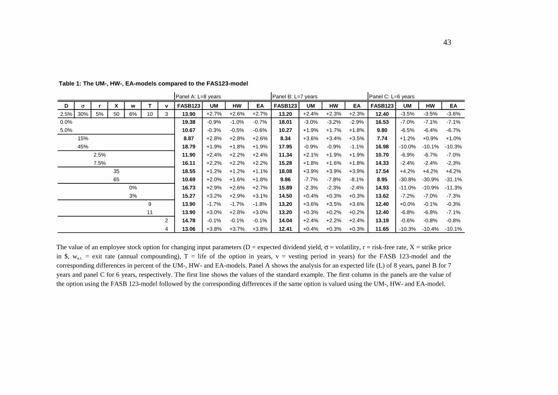
Table 1 shows a comparison of the four models FASB 123, UM, HW and EA. The value of
an option for changing input parameters are calculated and calibrated to a certain expected
life. Prices are calibrates to expected lives of 8, 7, and 6 years, displayed in adjacent panels
possible that the stock price is well above the critical value at the end of the vesting period and, on the other hand, exercise will take place for all stock prices above the exercise price at the end of the option's life. 16 The average of the ratio between the stock price at the time of exercise and the strike price of 2.75 seems somewhat high given an average appreciation ratio of 1.7 of the S&P500 Composite index within a rolling window of 5.83 years between 1979 and 1994. This indicates that the performance of the firms in the Carpenter (1998) sample is unusually high.
21
A, B, and C, respectively. The differences in percentage prices refer to the FASB 123
model, which serves as a benchmark, displayed in the leftmost column of each panel.
The differences between the FASB 123 model and the other models appear to be fairly
small, at least for expected lives of 8 and 7 years, where percentage deviations remain
within single digits. However, as Panel C shows, the differences between the FASB 123
model and the UM, HW-, and EA-models increase significantly for an expected life of 6
years, where they can be as high as -31.1% for out-of-the-money options considered in this
table. Particularly a higher volatility, a higher strike price, a smaller exit rate, and a higher
vesting period lead to different option values for the FASB 123 model compared to the
three other models. The results in Table 1 are consistent with Figure 4, where the FASB
123-model’s substantial deviation from other models can be seen very clearly. Table 1 also
shows that the sign of the deviation is usually the same for UM, HW, and EA models.
Table 2 shows a comparison of the three models UM, HW and EA. As before, the value of
an option for changing input parameters is calculated and calibrated for a certain expected
life. The percentage differences in Table 2 refer to the HW-model, which serves as a
benchmark. As Table 2 shows, the three models produce nearly the same values for the
employee stock options when the expected life for a set of input parameters is fixed. There
are very small differences between the three models in the range of –0.4% to +0.4%. A
more extensive numerical analysis confirmed that this result pertains also for other
parameter combinations not displayed in the table. Thus, the conclusion can be drawn that
the three models are almost numerically equivalent if they are calibrated to the same
expected life.

22
Table 3 presents a sensitivity analysis for the four models. It shows that the sensitivities are
similar for all four models. However, the FASB 123 model responds sometimes rather
differently compared to the three other models, especially for a smaller expected life,
confirming earlier observations. Volatility, expected dividend yield, and moneyness (strike
price) are the parameters where the employee stock option value is most sensitive,
followed by the exit rate, risk-free rate, vesting period and life of the option. The analysis
in this section shows that the interpretations of Figure 4 can be generalized to other option
specifications and other parameter combinations.
[Table 1]
[Table 2]
[Table 3]
6 State-Dependent Exit Rate
In this section, we quantify the impact of a time-varying exit rate during the pre-vesting
period. Previously, the exit rate was assumed to be constant. This may not be a realistic
assumption because employees will be less likely to leave the firm if they own a significant

23
number of in-the-money options vesting soon than if those options are deeply “under
water” (out-of-the-money)17. Therefore, if the employee stock option is in the money
during the vesting period, the exit rate is reduced because the employee has an incentive to
wait for the options to vest and thus not leave the firm voluntarily during this time18. A
model that allows for a state-dependent exit rate is not equivalent to other models that do
not contain this feature. Therefore, the following model with its state-dependent exit rate is
not directly comparable to the models proposed above.
We present a simple and easily implemented procedure for modifying the pre-vesting exit
rate. The procedure can be directly applied to the models discussed in Section 3. During
the vesting period, a new parameter m reduces the exit rate w if the option is in the money
at that node of the binomial tree. We refer to this adjustment as the modified (pre-vesting)
exit rate m w⋅ . The exit rate w after the vesting period and if the option is out-of-the-
money remains the same.
The decision rule for calculating the value of the employee stock option for the modified
UM-, HW-, as well as the EA-model adjusted19 during the vesting period (if ∆ <i t v ) is
modified according to20
, 1, 1 1,[ (1 ) ]m w t r ti j i j i jf e e p f p f− ⋅ ∆ − ∆
+ + += ⋅ ⋅ ⋅ + − ⋅ (6.1)
17 See for example Cuny and Jorion (1995) and Jennergren and Naslund (1993). 18 We neglect the likely conjecture that the probability of forfeiture may be positively correlated with the time remaining to the end of the vesting period, as pointed out by Rubinstein (1995). 19 The FASB 123 model cannot be adjusted in the same way, otherwise the modified FASB 123 model would be equal to a modified AM Ex&Vest-model adjusted for the expected life.
24
[Table 4]
Table 4 illustrates the impact of a changing exit rate on the value of the employee options.
All figures refer to the standard example from before and to expected lives of
approximately 8, 7, and 6 years (Panels A, B, and C, respectively). In each panel, the exit
rate is alternatively reduced to 3% or 0% during the vesting period if the option is in-the-
money. Table 4 shows that the effect of a reduced exit rate is non-negligible. It is possible
that the value of an employee stock option increases by as much as 15%. It can be shown
that for other input parameters (S, X, D, r, σ, T, v, w and different expected life), similar
results pertain. For example, if at time 0 the option is in the money (e.g. X=$35, S=$50 in
the standard example) value increases of up to 18.3% can occur. This analysis
demonstrates that a constant exit rate may underestimate the value of employee options by
a significant margin as employees change their exit behavior to maximize the value of their
compensation.
7 Conclusion
We have presented a comparative analysis of current models for employee stock options.
In particular, we have analyzed the model proposed by the Financial Accounting Standards
Board (1995), a utility-maximizing model as proposed by Kulatilaka and Marcus (1994),
20 For a detailed variables description see Appendix A.

25
Huddart (1994) and Rubinstein (1995), a recent model by Hull and White (2002, 2004),
and a new model (Enhanced American) proposed in this paper.
We found that the differences among the utility-maximizing, Hull-White, and Enhanced
American-models are minimal. Only the FASB 123 model produces different prices. To
make those models comparable, we used a common implicit parameter, the expected life of
the option, and calibrated the models to this parameter. We showed that, for parameter
combinations implying the same expected option life, the price differences are extremely
small for all parameter combinations tested. In other words, the exercise scheme generated
by a particular model is relevant only to the extent it affects the expected life of the option.
The pricing effect of differences in the exercise schemes resulting in the same expected life
is minimal.
Furthermore, for the utility-maximizing model, we found that arbitrarily chosen
combinations of the utility-relevant parameters, such as risk aversion, expected return, and
non-option wealth, produce identical option prices if they imply the same expected life of
the option. Therefore, by using the expected life of the option as an implicit parameter, the
utility-maximizing model, which relies on unobservable and hard to estimate parameters,
can be simplified in its application because, instead of the original model parameters, only
the expected life parameter needs to be estimated.
As a further contribution, we show that modeling a time-varying employee exit rate can
increase the value of the option if it is assumed that the exit rate decreases during the

26
vesting period if the option is in-the-money. Hence, valuation models using constant exit
rates tend to underestimate the value of employee options.
Acknowledgement
We would like to thank Bernd Brommundt, Michael Genser, Stephan M. Kessler, Peter
Raupach and Michael Verhofen for their helpful comments.
References
Carpenter, J. 1998. ”The exercise and valuation of executive stock options.” Journal of
Financial Economics, vol. 48, no. 2:127-158.
Cuny, J.C., and P. Jorion. 1995. ”Valuing executive stock options with endogenous
departure.” Journal of Accounting and Economics, vol. 20, no. 2:193-205.
Cox, J.C., Ross S. and M. Rubinstein. 1979. “Option Pricing: A Simplified Approach.”
Journal of Financial Economics, vol. 7, no. 3:229-263.
DeTemple, J. and S. Sundaresan. 1999. ”Nontraded asset valuation with portfolio
constraints: A binomial approach.” The Review of Financial Studies, vol. 12, no. 4:835-
872.
Financial Accounting Standards Board. 1995. “FASB 123: Accounting for Stock-Based
Compensation."
Garman, M. 1989. “Semper Tempus Fugit.” RISK, vol. 2, no. 5 (May):34-35.

27
Hall, B.J. and K.J. Murphy. 2000. ”Optimal exercise prices for risk averse executives.”
American Economic Review, vol. 90, no. 2:209-214.
Hall, B.J. and K.J. Murphy. 2002. ”Stock options for undiversified executives.” Journal of
Accounting and Economics, vol. 33, no.1:3-42.
Hemmer, T. and S. Matsunaga. 1994. “Estimating the ‘Fair Value’ of Employee Stock
Options with Expected Early Exercise.” Accounting Horizons, vol. 8, no. 4:23-42.
Huddart, S. 1994. “Employee Stock Options.” Journal of Accounting and Economics, vol.
18, no. 2:207-231.
Huddart, S. and M. Lang. 1996. “Employee stock options exercises: An empirical
analysis.“ Journal of Accounting and Economics, vol. 21, no. 1:5-43.
Hull, J. and A. White. 2002. “Determining the Value of Employee Stock Options.” Report
Produced for the Ontario Teachers Pension Plan.
Hull, J. and A. White. 2003. “Accounting for Employee Stock Options.” Working Paper,
University of Toronto.
Hull, J. and A. White. 2004. “How to value Employee Stock Options.” Financial Analysts
Journal, vol. 60, no. 1:114-119.
Jennergren, L. and B. Naslund. 1993. “A comment on ‘Valuation of executive stock
options and the FASB proposal’.” The Accounting Review, vol. 68, no.1:179-183.
Kulatilaka, N. and A. J. Marcus. 1994. “Valuing Employee Stock Options.” Financial
Analyst Journal, vol. 50, no. 6:46-56.
Lambert, R.A. and D.F. Larcker and R. E. Verrecchia. 1991. ”Portfolio considerations in
valuing executive compensation.” Journal of Accounting Research, vol. 29, no. 1:129-
149.

28
Rubinstein, M. 1995. “On the Accounting Valuation of Employee Stock Options. ” Journal
of Derivatives, vol. 3, no. 1:8-24.
Smith, C. W. and J. L. Zimmerman. 1976. ”Valuing employee stock option plans using
option pricing models.” Journal of Accounting Research, vol. 14, no.2 (Autumn):357-364.
29
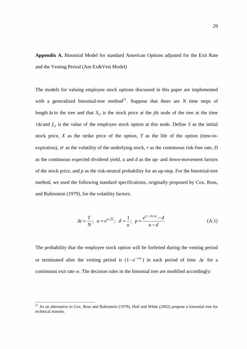
Appendix A. Binomial Model for standard American Options adjusted for the Exit Rate
and the Vesting Period (Am Ex&Vest Model)
The models for valuing employee stock options discussed in this paper are implemented
with a generalized binomial-tree method21. Suppose that there are N time steps of
length ∆t in the tree and that Si,j is the stock price at the jth node of the tree at the time
∆i t and fi,j is the value of the employee stock option at this node. Define S as the initial
stock price, X as the strike price of the option, T as the life of the option (time-to-
expiration), σ as the volatility of the underlying stock, r as the continuous risk-free rate, D
as the continuous expected dividend yield, u and d as the up- and down-movement factors
of the stock price, and p as the risk-neutral probability for an up-step. For the binomial-tree
method, we used the following standard specifications, originally proposed by Cox, Ross,
and Rubinstein (1979), for the volatility factors:
( )1
; ; ; − ⋅∆
σ ∆ −∆ = = = =−
r D ttT e d
t u e d pN u u d
(A.1)
The probability that the employee stock option will be forfeited during the vesting period
or terminated after the vesting period is (1 − ∆− w te ) in each period of time ∆t for a
continuous exit rate w. The decision rules in the binomial tree are modified accordingly:
21 As an alternative to Cox, Ross and Rubinstein (1979), Hull and White (2002) propose a trinomial tree for technical reasons.
30
The value of the employee stock option in each node of the tree is denoted by fi,j for time i
and node j. At maturity of the option (i=N), the value of the option is given as the option’s
intrinsic value , ,max( ,0)= −N j N jf S X . For all other nodes ( 0 1≤ ≤ −i N ), the rules are as
follows:
─ During the vesting period (if ∆ <i t v ):
If there is an exit, occurring with probability (1 − ∆− w te ), the option will be forfeited
and the exit value equals 0. Therefore the component of the option price will be the
probability multiplied by the exit value: (1 ) 0 0w te− ∆− ⋅ = .
If there is no exit, occurring with probability − ∆w te , the option will be held and the
holding value using risk-neutral valuation gives 1, 1 1,[ (1 ) ]r ti j i je p f p f− ∆+ + +⋅ ⋅ + − ⋅ .
Therefore, the component of the option price will be the probability multiplied by
the holding value: 1, 1 1,[ (1 ) ]w t r ti j i je e p f p f− ∆ − ∆+ + +⋅ ⋅ ⋅ + − ⋅ .
The value of the option is the sum of these two components (exit and no exit), i.e.,
, 1, 1 1,
0
(1 ) 0 [ (1 ) ]w t w t r ti j i j i jf e e e p f p f− ∆ − ∆ − ∆
+ + +
=
= − ⋅ + ⋅ ⋅ ⋅ + − ⋅14243
(A.2)
─ After the vesting period (if ∆ ≥i t v ):

31
If there is an exit with probability (1 − ∆− w te ), the option will be exercised
immediately and the exit value is given by the option’s intrinsic value, namely
,max( ,0)i jS X− . Therefore, the component of the option price will be the
probability multiplied by the exit value: ,(1 ) max( ,0)w ti je S X− ∆− ⋅ − .
If there is no exit with probability − ∆w te , the option will either be exercised or held:
If the option will be exercised: the component of the option price will be
,max( ,0)w ti je S X− ∆ ⋅ − .
If the option will be held: the component of the option price will be
1, 1 1,[ (1 ) ]w t r ti j i je e p f p f− ∆ − ∆+ + +⋅ ⋅ ⋅ + − ⋅ .
The value of the option is the sum of these two components (exit and no exit):
If the option will be exercised:
, , ,
,
(1 ) max( ,0) max( ,0)
max( ,0)
w t w ti j i j i j
i j
f e S X e S X
S X
− ∆ − ∆= − ⋅ − + ⋅ −
= − (A.3)
If the option will be held:
, , 1, 1 1,(1 ) max( ,0) [ (1 ) ]w t w t r ti j i j i j i jf e S X e e p f p f− ∆ − ∆ − ∆
+ + += − ⋅ − + ⋅ ⋅ ⋅ + − ⋅ (A.4)
We refer to the binomial model for standard American options as AM-model and the
binomial model adjusted for the exit rate and the vesting period as described above as AM
Ex&Vest-model.
32
Appendix B. Expected Life
In this appendix, the calculation of the risk-neutral expected life is described. Define ,i jL
as the risk-neutral expected life of the option at time i t∆ . The stock price is ,i jS . Set
, 0N jL = for the expected life at the end nodes. For all other nodes ( 0 1≤ ≤ −i N ), expected
life is calculated as follows:
─ During the vesting period (if ∆ <i t v ), the option cannot be exercised and,
according to the risk-neutral valuation principle, the expected life, for a time
increase of one binomial step ( t∆ ), is calculated as (recall that the exit rate is
ignored because the expectation is conditional)
, 1, 1 1,(1 )i j i j i jL p L p L t+ + += ⋅ + − ⋅ + ∆ . (B.1)
─ After the vesting period (if ∆ ≥i t v ), expected life is calculated as follows:
If the option is exercised, then
, 0i jL = . (B.2)
If the option is held, then22
, 1, 1 1,
0
(1 ) 0 [ (1 ) ]w t w ti j i j i jL e e p L p L t− ∆ − ∆
+ + +
=
= − ⋅ + ⋅ ⋅ + − ⋅ + ∆14243
(B.3)
The expected life of an option today, i.e., in the first node, is L0,0.
22 Hull and White (2002) use ∆w t instead of (1 )− ∆− w te .

33
Appendix C. The Utility Maximization Model
The rules for calculating the utility in each node ( 0 1≤ ≤ −i N ) are as follows:
If the option is held, the utility at the node (i, j), ,H
i jU is the conditional expectation
using the probability π, i.e.,
, 1, 1 1,(1 )+ + += π⋅ + − π ⋅Hi j i j i jU U U . (C.1)
If the option is exercised, the utility at the node (i, j), ,E
i jU is defined as the utility
of the non-option wealth plus the cash realized from exercising the option, both
invested in risk-free assets, giving
( )
, 0 ,( [max( ,0)] )−
⋅= ⋅ + − ⋅N i
rTE r T Ni j i jU U W e S X e (C.2)
─ During the vesting period (if ∆ <i t v ), where the option cannot be exercised, the utility
,i jU is defined as the probability of no exit − ∆w te multiplied by the utility in the case of
holding the option plus the probability of an exit (1 )− ∆− w te multiplied by the utility of
the non-option wealth invested in risk-free assets only. This gives
, , 0(1 ) ( )− ∆ − ∆= ⋅ + − ⋅ ⋅Hw t w t rTi j i jU e U e U W e . (C.3)

34
─ After the vesting period (if ∆ ≥i t v ) and if there is no exit with probability − ∆w te , the
exercise scheme is determined by the maximum of the utility if the option is exercised
,E
i jU and the utility if the option is held ,H
i jU . If there is an exit with probability
(1 )− ∆− w te , the utility is given as the exercise utility ,E
i jU , i.e.,
, , , ,max[ , ] (1 )− ∆ − ∆= ⋅ + − ⋅E H Ew t w ti j i j i j i jU e U U e U . (C.4)
This utility tree determines the individual exercise scheme of the employee. Using the
exercise scheme and working backward through the tree, the value of the option, UMf , can
be determined. In the end nodes the value of the option is given as the option’s intrinsic
value, , ,max( ,0)= −N j N jf S X . For all other nodes ( 0 1≤ ≤ −i N ) the rules are as follows:
─ During the vesting period (if ∆ <i t v ) the value of the option is calculated as:
, 1, 1 1,[ (1 ) ]− ∆ − ∆+ + += ⋅ ⋅ ⋅ + − ⋅w t r t
i j i j i jf e e p f p f . (C.5)
─ After the vesting period (if ∆ ≥i t v ):
If the option is exercised, then the value of the option is its intrinsic value, i.e.,
, ,= −i j i jf S X . (C.6)

35
If the option is held, then the value is
, , 1, 1 1,(1 ) max( ,0) [ (1 ) ]w t w t r ti j i j i j i jf e S X e e p f p f− ∆ − ∆ − ∆
+ + += − ⋅ − + ⋅ ⋅ ⋅ + − ⋅ . (C.7)
The value of the option at time 0 is given as 0,0f .
36
Appendix D. The Hull-White Model
The rules for calculating the value of the option are as follows23: At the end nodes the
value of the option is given as the option’s intrinsic value , ,max( ,0)= −N j N jf S X , and for
all other nodes ( 0 1i N≤ ≤ − ), the rules are:
─ During the vesting period (if ∆ <i t v ), the value of the option is calculated as
, 1, 1 1,[ (1 ) ]w t r ti j i j i jf e e p f p f− ∆ − ∆
+ + += ⋅ ⋅ ⋅ + − ⋅ . (D.1)
─ After the vesting period (if ∆ ≥i t v ):
If ,i jS X M≥ ⋅ (stock price above or equal exercise criterion), then the
option will be exercised, i.e.,
, ,i j i jf S X= − . (D.2)
If ,i jS X M< ⋅ (stock price below exercise criterion) then the option will be
held, i.e.,
23 Hull and White (2002, 2003) propose w1 as the employee exit rate during the vesting period and w2 as the
employee exit rate after the vesting period and they use 1 iw t
iw t e
− ∆∆ = − for 1, 2i = . For comparison reasons
we assume that w1=w2=w.

37
, ,
1, 1 1,
(1 ) max( ,0)
[ (1 ) ]
w ti j i j
w t r ti j i j
f e S X
e e p f p f
− ∆
− ∆ − ∆+ + +
= − ⋅ −
+ ⋅ ⋅ ⋅ + − ⋅ (D.3)
The value of the option is 0,0f .

38
Appendix E. The Enhanced American Model
The rules for calculating the value of the option 0,0f are: At the end nodes the value of the
option is given as the option’s intrinsic value , ,max( ,0)= −N j N jf S X . For all other nodes
( 0 1i N≤ ≤ − ), the rules for calculating the value of the employee stock option are as
follows:
─ During the vesting period (if ∆ <i t v ), the value of the option is calculated as
, 1, 1 1,[ (1 ) ]w t r ti j i j i jf e e p f p f− ∆ − ∆
+ + += ⋅ ⋅ ⋅ + − ⋅ . (E.1)
─ After the vesting period (if ∆ ≥i t v ):
If there is a positive intrinsic value (i.e. , 0i jS X− > ) and the exercise
criterion, i.e.,
*, 1, 1 1,max( ,0) [ (1 ) ]r t
i j i j i jS M X e pf p f− ∆+ + +− ⋅ ≥ ⋅ + − , (E.2)
is satisfied, then the option will be exercised. Its value is therefore
, , ,max( ,0)i j i j i jf S X S X= − = − . (E.3)
Otherwise, the option is held and its value is therefore

39
, ,
1, 1 1,
(1 ) max( ,0)
[ (1 ) ]
w ti j i j
w t r ti j i j
f e S X
e e p f p f
− ∆
− ∆ − ∆+ + +
= − ⋅ −
+ ⋅ ⋅ ⋅ + − ⋅ (E.4)

40
Value of employee stock options with respect to the expected life of the option (S = $50, X = $50, σ = 30%, r = 5%, D = 2.5%, T = 10 years, wa.c. = 6%, v = 3 years). The 1331values are calculated using changing risk aversion from the set [0, 1, 2, .., 9, 10], changing expected stock return from the set [5%, 5.5%, .., 9.5%, 10%] and changing non-option wealth from the set [$0, $20, $40, .., $180, $200].
8
9
10
11
12
13
14
15
4 5 6 7 8 9 10
Expe cte d Life (Years )
Val
ue
of
the
Op
tio
n (
$)Figure 1. Utility Maximization Model
Figure 2. Hull-White Model
Value of employee stock options with respect to the multiple M; (S = $50, X = $50, σ = 30%, r = 5%, D = 2.5%, T = 10 years, wa.c. = 6%, v = 3 years). The limit is given by the American model adjusted for the exit rate and the vesting period.
13.5
13.6
13.7
13.8
13.9
14
14.1
14.2
14.3
14.4
14.5
1 2 3 4 5 6 7 8 9 10
Multiple M
Val
ue
of
the
Op
tio
n (
$)
Hull-White Am Ex&Vest

41
Value of employee stock options with respect to the expected life (S = $50, X = $50, σ = 30%, r = 5%, D = 2.5%, T = 10 years, wa.c. = 6%, v = 3 years).
8
10
12
14
16
18
0 2 4 6 8 10Expected Life (Years)
Val
ue
of
the
Op
tio
n (
$)
AM Ex&Vest
AM Ex
AM AM Vest
B/S
FASB 123
UM, HW and EA
Figure 4. Comparison of the employee stock option valuation models
13.5
13.6
13.7
13.8
13.9
14.0
14.1
14.2
14.3
14.4
14.5
0.97 0.99 1.01 1.03 1.05
Multiple M*
Val
ue
of
the
Op
tio
n (
$)
Enhanced American Am Ex&Vest
Figure 3. Enhanced American Model
Value of employee stock options with respect to the multiple M* that triggers an earlier or delayed exercise (S = $50, X = $50, σ = 30%, r = 5%, D = 2.5%, T = 10 years, wa.c. = 6%, v = 3 years). The limit is given by the American model adjusted for the exit rate and the vesting period.

42
excercise region
Boundary of the HW-model
Boundary of the UM-model
Boundary of the EA-model
Time (Years) 0 10
Vesting
Sto
ck P
rice
Figure 5. Schematic binomial tree with exercise boundaries
Graphical representation of the schematic exercise boundaries for the HW-/ UM- and EA-model for the standard example (S = $50, X = $50, σ = 30%, r = 5%, D = 2.5%, T = 10 years, wa.c. = 6%, v = 3 years). Expected life is set to 7.04 years.
43
The value of an employee stock option for changing input parameters (D = expected dividend yield, σ = volatility, r = risk-free rate, X = strike price in $, wa.c. = exit rate (annual compounding), T = life of the option in years, v = vesting period in years) for the FASB 123-model and the corresponding differences in percent of the UM-, HW- and EA-models. Panel A shows the analysis for an expected life (L) of 8 years, panel B for 7 years and panel C for 6 years, respectively. The first line shows the values of the standard example. The first column in the panels are the value of the option using the FASB 123-model followed by the corresponding differences if the same option is valued using the UM-, HW- and EA-model.
Table 1: The UM-, HW-, EA-models compared to the FAS123-model
Panel A: L=8 years Panel B: L=7 years Panel C: L=6 years
D σ r X w T v FASB123 UM HW EA FASB123 UM HW EA FASB123 UM HW EA
2.5% 30% 5% 50 6% 10 3 13.90 +2.7% +2.6% +2.7% 13.20 +2.4% +2.3% +2.3% 12.40 -3.5% -3.5% -3.6%
0.0% 19.38 -0.9% -1.0% -0.7% 18.01 -3.0% -3.2% -2.9% 16.53 -7.0% -7.1% -7.1%
5.0% 10.67 -0.3% -0.5% -0.6% 10.27 +1.9% +1.7% +1.8% 9.80 -6.5% -6.4% -6.7%
15% 8.87 +2.8% +2.8% +2.6% 8.34 +3.6% +3.4% +3.5% 7.74 +1.2% +0.9% +1.0%
45% 18.79 +1.9% +1.8% +1.9% 17.95 -0.9% -0.9% -1.1% 16.98 -10.0% -10.1% -10.3%
2.5% 11.90 +2.4% +2.2% +2.4% 11.34 +2.1% +1.9% +1.9% 10.70 -6.9% -6.7% -7.0%
7.5% 16.11 +2.2% +2.2% +2.2% 15.28 +1.8% +1.6% +1.8% 14.33 -2.4% -2.4% -2.3%
35 18.55 +1.2% +1.2% +1.1% 18.08 +3.9% +3.9% +3.9% 17.54 +4.2% +4.2% +4.2%
65 10.69 +2.0% +1.6% +1.8% 9.86 -7.7% -7.8% -8.1% 8.95 -30.8% -30.9% -31.1%
0% 16.73 +2.9% +2.6% +2.7% 15.89 -2.3% -2.3% -2.4% 14.93 -11.0% -10.9% -11.3%
3% 15.27 +3.2% +2.9% +3.1% 14.50 +0.4% +0.3% +0.3% 13.62 -7.2% -7.0% -7.3%
9 13.90 -1.7% -1.7% -1.8% 13.20 +3.6% +3.5% +3.6% 12.40 +0.0% -0.1% -0.3%
11 13.90 +3.0% +2.8% +3.0% 13.20 +0.3% +0.2% +0.2% 12.40 -6.8% -6.8% -7.1%
2 14.78 -0.1% -0.1% -0.1% 14.04 +2.4% +2.2% +2.4% 13.19 -0.6% -0.8% -0.8%
4 13.06 +3.8% +3.7% +3.8% 12.41 +0.4% +0.3% +0.3% 11.65 -10.3% -10.4% -10.1%

44
The value of an employee stock option for changing input parameters (D = expected dividend yield, σ = volatility, r = risk-free rate, X = strike price
in $, wa.c. = exit rate (annual compounding), T = life of the option in years, v = vesting period in years) for the HW-model and the corresponding differences in percent of the UM- and EA-models. Panel A shows the analysis for an expected life (L) of 8 years, panel B for 7 years and panel C for 6 years, respectively. The first line shows the values of the standard example. The first column in the panels is the value of the option using the HW- model followed by the corresponding differences if the same option is valued using the UM- and the EA-model.
Table 2: The UM- and EA-models compared to the HW-model
Panel A: L=8 years Panel B: L=7 years Panel C: L=6 years
D σ r X w T v HW UM EA HW UM EA HW UM EA
2.5% 30% 5% 50 6% 10 3 14.26 +0.1% +0.1% 13.50 +0.1% +0.1% 11.97 +0.0% -0.2%
0.0% 19.18 +0.1% +0.4% 17.44 +0.2% +0.3% 15.36 +0.1% -0.1%
5.0% 10.62 +0.2% -0.1% 10.44 +0.2% +0.1% 9.17 -0.1% -0.3%
15% 9.12 +0.0% -0.2% 8.62 +0.2% +0.1% 7.81 +0.3% +0.1%
45% 19.12 +0.2% +0.2% 17.79 +0.0% -0.2% 15.27 +0.1% -0.3%
2.5% 12.16 +0.2% +0.2% 11.56 +0.2% +0.0% 9.98 -0.2% -0.3%
7.5% 16.46 +0.0% +0.0% 15.53 +0.2% +0.1% 13.98 +0.0% +0.1%
35 18.78 +0.0% -0.1% 18.78 +0.1% +0.1% 18.27 +0.1% +0.1%
65 10.86 +0.4% +0.2% 9.09 +0.1% -0.3% 6.18 +0.2% -0.2%
0% 17.16 +0.3% +0.1% 15.53 +0.0% -0.1% 13.30 -0.1% -0.4%
3% 15.72 +0.3% +0.2% 14.54 +0.1% +0.0% 12.66 -0.2% -0.3%
9 13.67 +0.0% -0.1% 13.66 +0.1% +0.1% 12.39 +0.1% -0.2%
11 14.29 +0.2% +0.2% 13.22 +0.2% +0.1% 11.56 +0.0% -0.3%
2 14.77 +0.0% +0.0% 14.35 +0.2% +0.2% 13.09 +0.2% +0.0%
4 13.54 +0.1% +0.1% 12.45 +0.1% +0.0% 10.44 +0.1% +0.3%

45
The value of an employee stock option for changing input parameters (D = expected dividend yield, σ = volatility, r = risk-free rate, X = strike price in $, wa.c. = exit rate (annual compounding), T = life of the option in years, v = vesting period in years) for the FASB 123-, UM-, HW- and EA-models Panel A shows the analysis for an expected life (L) of 8 years, Panel B for 7 years and Panel C for 6 years, respectively. The first line shows the values of the standard example. The columns in the panels are the differences between the value of the standard option and the value of the option with changed input parameters.
Table 3: Sensitivity analysis for the FASB123-, UM-, HW-, EA-models
Panel A: L=8 years Panel B: L=7 years Panel C: L=6 years
D σ r X w T v FASB123 UM HW EA FASB123 UM HW EA FASB123 UM HW EA
2.5% 30% 5% 50 6% 10 3 13.90 14.28 14.26 14.27 13.20 13.52 13.50 13.51 12.40 11.97 11.97 11.950.0% +39.4% +34.5% +34.5% +34.9% +36.4% +29.2% +29.2% +29.5% +33.3% +28.4% +28.3% +28.5%
5.0% -23.2% -25.5% -25.5% -25.6% -22.2% -22.6% -22.7% -22.6% -21.0% -23.5% -23.4% -23.5%
15% -36.2% -36.1% -36.0% -36.2% -36.8% -36.1% -36.1% -36.1% -37.6% -34.6% -34.8% -34.6%
45% +35.2% +34.1% +34.1% +34.2% +36.0% +31.6% +31.8% +31.4% +36.9% +27.7% +27.6% +27.4%
2.5% -14.4% -14.6% -14.7% -14.6% -14.1% -14.3% -14.4% -14.4% -13.7% -16.8% -16.6% -16.7%
7.5% +15.9% +15.3% +15.4% +15.3% +15.8% +15.1% +15.0% +15.1% +15.6% +16.8% +16.8% +17.2%
35 +33.5% +31.5% +31.7% +31.5% +37.0% +39.0% +39.1% +39.1% +41.5% +52.7% +52.6% +53.0%
65 -23.1% -23.7% -23.8% -23.8% -25.3% -32.7% -32.7% -32.9% -27.8% -48.3% -48.4% -48.4%
0% +20.4% +20.5% +20.3% +20.4% +20.4% +14.9% +15.0% +14.8% +20.4% +11.0% +11.1% +10.9%
3% +9.9% +10.4% +10.2% +10.4% +9.8% +7.7% +7.7% +7.6% +9.8% +5.6% +5.8% +5.6%
9 +0.0% -4.3% -4.1% -4.3% +0.0% +1.2% +1.2% +1.3% +0.0% +3.6% +3.5% +3.4%
11 +0.0% +0.3% +0.2% +0.4% +0.0% -2.1% -2.1% -2.1% +0.0% -3.4% -3.4% -3.6%
2 +6.3% +3.4% +3.6% +3.5% +6.4% +6.4% +6.3% +6.4% +6.4% +9.5% +9.4% +9.5%
4 -6.0% -5.0% -5.0% -5.0% -6.0% -7.8% -7.8% -7.8% -6.0% -12.7% -12.8% -12.4%

46
Table 4. Modified Pre-Vesting Exit Rate
Modified Exit Rate Modified UM Modified HW Modified EA
Panel A: Excepted Life = 7.99
6.0% 14.27 14.26 14.27
3.0% +7.0% +7.0% +7.0%
0.0% +14.6% +14.6% +14.6%
Panel B: Excepted Life = 7.04
6.0% 13.57 13.55 13.56
3.0% +7.0% +7.0% +7.1%
0.0% +14.6% +14.6% +14.7%
Panel C: Excepted Life = 5.95
6.0% 11.87 11.88 11.86
3.0% +7.2% +7.2% +7.2%
0.0% +15.0% +15.0% +15.0%
The first line of Panel A, B and C shows the values of the option for the unchanged pre-vesting exit rate. The post-vesting exit rate remains constant at 6%. The values are calculated for the standard example:
S = $50; X = $50; D = 2.5%; r = 5%; σ = 30%; T = 10 years; v = 3 years; wa.c. = 6%