Does the Launch of the Euro Hinder the Current Account Adjustment of the

Eurozone?

Jo-wei Wu

Assistant Research Fellow

Chung-Hua Institution for Economic Research, Taipei, Taiwan

Email: roweiwu9@yahoo.com.tw

Jyh-Lin Wu*

Professor

Institute of Economics, National Sun Yat-sen University, Taiwan.

Email: jlwu2@mail.nsysu.edu.tw

Department of Economics, National Chung Cheng University, Taiwan.

Email:ecdjlw@ccu.edu.tw

* Corresponding author. We are grateful to William Branch (Co-editor) and two

anonymous referees for very valuable comments and suggestions on the previous

version of the paper. Our appreciation also go to seminar participants at the 2016

Asian and Chinese Meeting of Econometric Society. Remaining Errors are our own.

1  

Does the Launch of the Euro Hinder the Current Account Adjustment of the

Eurozone?

Abstract This paper examines current account adjustments before and after the launch of the

euro. After controlling for nonlinear smooth changes in mean, contemporaneous

dependence of disturbances, and the finite sample bias of estimates, we provide robust

evidence to support that the adoption of the euro facilitates rather than hinders the

adjustment of current accounts. This finding agrees with our results that the use of the

euro assists real exchange rate and inflation rate adjustments.

Keywords: current accounts, real exchange rates, contemporaneous dependence,

half-life, exchange rate regimes.

JEL: C33, F32 , F41.

1. Introduction

The advocates of a flexible exchange-rate system highlight the usefulness of

flexible exchange rates to promote the adjustment of international relative prices

towards equilibrium even when goods prices are sticky (Friedman, 1953). This is

because nominal exchange rate changes are easier and more efficient than price

changes. Under a fixed exchange-rate regime, the adjustment depends entirely on

sticky goods and factor prices. Therefore, a country’s current account is supposed to

reveal a faster adjustment under a flexible exchange-rate regime than under a

fixed-rate regime. The empirical support of the above Friedman hypothesis has an

important policy recommendation of using exchange rate flexibility to reduce current

account imbalances. However, there is no general consensus on the link between the

exchange rate regime and current account adjustment.

The purpose of this paper is to re-examine whether the speed of current account

adjustment is systematically associated with a country’s nominal exchange rate

flexibility. The paper differs from the existing literature in several important ways.

First, we specify a dynamic panel model that allows for regime-specific nonlinear

smooth changes in the equilibrium level of the current account, which are supported

by theoretical explanations and a pre-test model specification. Allowing nonlinear

2  

smooth changes in the equilibrium level is important since parameter estimates suffer

the omitted-variable bias if they appear in data but are ignored in estimation. Second,

controlling for contemporaneous dependence of disturbances is important in panel

data estimation but it is generally ignored in standard panel data estimators such as the

least squares dummy variables (LSDV) and the pooling ordinary least squares (POLS)

estimators. The standard panel data estimators are inconsistent when disturbances are

contemporaneously correlated. To control for cross-sectional dependence of

disturbances, the common correlated effect pooled (CCEP) estimator of Pesaran

(2006) is applied to estimate the specified model. Furthermore, Kilian’s (1998) double

bootstrap method is applied to correct the finite sample bias of CCEP estimates due to

the inclusion of lagged dependent variables as regressors.1 Third, three key

components in our methodology are allowing nonlinear smooth shifts in mean,

controlling for cross-sectional dependence of disturbances, and correcting the finite

sample bias of estimates. This paper examines how failing to take into account these

components in methodology affects the results. Finally, we examine to what extent

these components account for the different conclusions in the literature.

We focus on the original countries in the eurozone over 1973-2015.2 These

countries used the floating exchange-rate regime (1973-1978) and the Exchange Rate

Mechanism (ERM, 1979-1998) regime before 1999 and switched to a completely

fixed-rate regime after the adoption of the common currency. We combine the float

rate regime before 1979 and the crawling pegged ERM regime from 1979 to 1998 into

a single regime.3 Hence, nominal exchange rates had some degree of flexibility

before 1999 (pre-euro period) and have been completely fixed since 1999 (euro

period). An important concern when examining the association between exchange rate

regimes and the dynamics of macro-variables is the regime endogeneity: the

possibility that the dynamics of current accounts drive exchange-rate regimes (Chinn

and Wei, 2013). This concern is no longer important in our case since the decision to

form the eurozone in 1991 was part of a broader historical process of European

economic integration.4 It is unlikely that current accounts among the eurozone

1 A Monte Carlo study of the bias of the CCEP estimator when a lag dependent variable appears in the model can be found in Bergin et al. (2013). 2 We restrict our discussion on the Friedman hypothesis under the pre-euro and euro periods since quarterly current account data are available starting from 1977 for most industrial countries. 3 As discussed in section 6, our empirical results are generally robust if the years of floating rate regime (1973-1978) are removed from the pre-euro period. 4 Major concerns for European economic integrations are to allow for the realization of economic

3  

countries in the pre-euro period influenced the decision to form the European

Currency Union (Ghosh et al., 2014).

Our empirical results first point out that the launch of the euro facilitates rather

than hinders current account adjustment. This result is surprising since it challenges

the Friedman hypothesis. To understand why our finding above is reasonable, we

examine the effects of exchange rate regimes on real exchange rate dynamics. Current

accounts respond to real exchange rates instead of nominal exchange rates. If real

exchange rates adjust faster in the euro period than in the pre-euro period, then current

accounts would adjust faster in the euro period than in the pre-euro period. We find

that the speed of real exchange rate reversal increases after the launch of the euro. A

theoretical explanation for the finding of faster current account and real exchange rate

adjustments under the euro period is that inflation adjustment is faster under the euro

period than under the pre-euro period (Alogoskoufis and Smith, 1991). Indeed, we

find that the adoption of the euro assists inflation adjustment, echoing the results

found from current accounts and real exchange rates. Furthermore, the above results

are robust to different scenarios.

How important are the three key components of our methodology in affecting

the results of the paper? We find that our results are not significantly affected even

though the finite sample bias of estimates is not corrected. However, current accounts

adjust faster instead of slower for the pre-euro period than the euro period, although

their difference is insignificant, when the model with a constant intercept is adopted,

and when standard panel estimation methods are adopted. The irrelevance of

exchange rate regimes to real exchange rate and inflation adjustments tends to be

observed when time-varying smooth equilibrium of variables is not allowed, when

contemporaneous dependence in disturbances is not controlled, and when standard

panel estimation methods are adopted.

The paper makes three contributions to the existing literature. First, our model

specification is a general one that nests existing specifications as special cases.

Second, the estimation method controls for contemporaneous dependence across

individuals and the finite sample bias of estimates, which are generally ignored in the

existing literature. Third, the Friedman hypothesis is examined by either using data

scales by removing non-tariff barriers, to result in allocative and productive efficiency gains by increasing competition in the market, and to achieve dynamic efficiency by increasing investment in product and process innovations.

4  

from current accounts or real exchange rates. We investigate the hypothesis using data

from current accounts, real exchange rates and inflation rates and provide consistent

evidence to oppose the hypothesis. The paper enhances our understanding of the

Friedman hypothesis.

The organization of the paper is given as follows. Section 2 reviews related

literature on current accounts and real exchange rates. Section 3 discusses model

specification and estimation methods, and Section 4 reports empirical results. Section

5 examines the importance of the three key components in our methodology. Section

6 discusses the robustness of our results. Finally, the last section concludes.

2. Related Literature

Related literature in current accounts and real exchange rates is too large to be

comprehensively reviewed here. We focus on recent literature that applies panel data

analysis.5 Many articles apply de facto exchange rate classification schemes to

examine whether a more rapid adjustment in current accounts occurs under more

flexible exchange rate regimes.6 Using a panel of 170 countries over the 1971-2005

period, Chinn and Wei (2013, 2008) present the first empirical study that

systematically tests the Friedman hypothesis and find no strong and robust link

between exchange rate regimes and the adjustment of the ratios of current accounts

over gross domestic products (GDP) (called current accounts hereafter). Clower and

Ito (2011) find similar results based on a panel of 70 countries.7 On the other hand,

using a panel of 151 countries from 1980-2007, Ghosh et al. (2010) find that, when

allowing for the threshold effect of large imbalances, exchange rate regimes seem to

be highly relevant for current account dynamics, in ways that generally support

Friedman’s argument.

Instead of using the above discrete de facto classifications, several authors

measure exchange rate regimes using exchange rate volatility based on Ghosh et al.

(2003). Applying a panel of 171 countries for 1970-2008, Tippkotter (2010) finds

faster current account convergence for more flexible exchange rate regimes when the

system GMM estimator of Blundell and Bond (1998) is applied. Using a

5 Clarida (2007) collected an excellent set of empirical articles on current account adjustment. 6 The differences among several well-known exchange rate regime classifications and the causes and consequences of a country’s choice of its exchange rate regime are reviewed in Rose (2011). 7 Several other papers indicate no straightforward relation between current account dynamics and exchange rate rigidity since the former can be driven by many other factors (Decressin and Stavrev, 2009; Ju and Wei, 2007).

5  

trade-weighted bilateral exchange rate volatility measure for 159 countries over 1980–

2010, Ghosh et al. (2013) show that exchange rate flexibility indeed matters for

current account dynamics. Herrmann (2009) focuses on 11 emerging economies in

central, eastern and south-eastern Europe from 1994-2007. Her empirical results

support the Friedman hypothesis.

Instead of using current accounts, some authors examine the Friedman

hypothesis via trade accounts. Berger and Nitch (2014) support Friedman’s argument

by finding that the degree of current account persistence is much higher for EMU

countries based on a panel of 18 European countries over the period 1948-2008.

Finally, Ghosh et al. (2014) point out the importance of differentiating the degree of

exchange rate flexibility across various trading partners and hence construct a novel

dataset of bilateral exchange rate regimes for 181 countries from 1980-2010. Using

their data set with bilateral trade account balances, Ghosh et al. (2014) support a

significant and robust relationship between exchange rate flexibility and the speed of

trade balance adjustment.8 In addition, they find that their findings are also supported

by several “natural experiments” of exogenous changes in exchange-rate regimes,

including the launch of the euro.

In short, the empirical supports for the Friedman hypothesis are mixed in the

existing literature, and the reasons are due to the differences in empirical methods,

data used, and the measure of exchange rate regimes. However, none of the above

literature control for contemporaneous dependence of residuals, regime-specific

nonlinear smooth shifts in mean, and the finite-sample bias of estimates.

There are also several papers that use real exchange rates to examine the

Friedman hypothesis of a positive association between exchange-rate flexibility and

real exchange rate adjustment; they obtain mixed results. Taylor (2002) shows no

clear-cut differences in the mean reversion behavior of real exchange rates across

exchange rate regimes. However, Parsley and Popper (2001) and Bergin et al. (2014)

show faster real exchange rate adjustment under a peg and hence oppose the Friedman

hypothesis. These articles did not examine the adjustment of real exchange rates

before and after the launch of the euro. Nor do they allow regime-specific nonlinear

smooth shifts in mean in their dynamic models. In addition, except for Bergin (2014),

8 The adjustment of bilateral trade balances could be very different from that of current account balances since a bilateral trade surplus between i and j and a bilateral trade deficit between i and k cancel out in aggregation causing smooth current account balances.

6  

they fail to control for contemporaneous dependence of disturbances and correct the

finite-sample bias of estimates. Although Bergin et al. (2014) did control for

contemporaneous dependence in disturbances and correct the finite-sample bias of

estimates, their model includes neither a trend nor smooth shifts in the intercept. They

focus on the persistence of real exchange rates over the period before and after the

Bretton Woods rather than the launch of the euro. They did not examine the

importance of their innovations in methodology to empirical results. Nor do they

examine the hypothesis using data on current accounts and inflation rates.

There are also several other papers focusing on the eurozone countries. Huang

and Yang (2015) apply a vector error correction model to examine the link between

exchange rate regimes and real exchange rate adjustment. They support the Friedman

hypothesis by finding the evidence for the mean reversion of real exchange rates

being weaker during the euro period than during the pre-euro period. Using micro

data of commodity prices, Parsely and Wei (2008) find no evidence of a significant

improvement in market integration due to the launch of the euro, implying that the

adoption of the euro does not facilitate real exchange rate adjustment. However, the

above two articles fail to consider the three key components in our methodology.

The paper by Bergin et al. (2016) is the one that is closest to our paper. They

develop a methodology that distinguishes between the roles of the nominal exchange

rate as an adjustment mechanism and as a source of shocks. They point out that the

launch of the euro facilitates real exchange rate adjustment, which contradicts the

Friedman hypothesis.9 There are several important differences between their paper

and ours. First, Bergin et al. (2016) focus on real exchange rate dynamics rather than

current account dynamics, and they apply monthly data instead of quarterly data.

Second, their model includes a trend but assumes no smooth shifts in the intercept.

Third, although Bergin et al. (2016) control for cross-sectional dependence of

disturbances and correct the bias of estimates, they do not examine how important

each of the components in their methodology is. Nor do they examine to what extent

these components account for different conclusions in the literature.

3. Model specifications and estimation methods

9 Half-life is the amount of time it takes for half of the current account (the real exchange rate) deviations to be eliminated (Steinsson, 2008). We set 1t to be the first period where the impulse

response function, h(t), falls from a value above 0.5 to a value below 0.5 in the subsequent periods. The half-life is 1t plus (h( 1t )-0.5)/(h( 1t )-h( 1t +1)).

7  

Does the adoption of the euro facilitate the adjustments of current accounts, real

exchange rates and inflation rates? A dynamic panel model with nonlinear smooth

shifts in mean is specified for these variables, respectively. The specified model is

then estimated by the CCEP estimator of Pesaran (2006), which controls for the

contemporaneous dependence of residuals. The finite sample bias of CCEP estimates

is corrected by Kilian’s (1998) method.

3.1 The specification of current accounts

Three interesting features appear in current accounts plotted in Figure 1. First,

time-varying means appear for each country’s current account in the sample. For

example, the 10-year means of the current account during the periods of

1979-1988,1989-1998 and 1999-2008 are -0.18%, -0.94% and 0.59% for Germany,

-0.08%, 0.09% and 0.06% for France, -0.16%, 1.03% and -0.61% for Italy and

-0.67%, 0.09% and 0.52% for the Netherlands. Second, current accounts appear to

have a trend, especially during the euro period. Third, significant current account

deficits appear for most countries during the years of the ERM crisis (1992-1993) and

the recent global financial crisis (2008-2011).

Theoretical explanations for the first two characteristics of current accounts are

provided. First, the global perspective of current accounts considers how differential

rates of return affect financial flows, exchange rates and the desired portfolio

allocation of wealth (Frenkel and Mussa, 1985; Mann, 2002). Hence, changes in

agents' perceptions regarding risk, portfolio allocation decisions, future fiscal policies,

and transaction costs in international financial flows, etc., could lead to smooth

changes in holding foreign assets and hence result in nonlinear smooth shifts in the

mean of current accounts (Christopoulos and Leo´n-Ledesma, 2010a; Leybourne and

Mizen, 1999).

Next, explaining a trending current account challenges theoretical models. Choi

et al. (2008) and Choi and Mark (2009) point out that a standard two-country dynamic

stochastic general equilibrium model with an endogenous discount factor is able to

generate a trend in current accounts. Besides, Chen et al. (2013) find that while

current account imbalances of euro area deficit countries vis-à-vis the rest of the

world increased, they were financed mostly by intra-euro area capital inflows, which

permitted external imbalances to grow over time. Based on the above discussion, we

apply an autoregressive process that incorporates a trend and nonlinear smooth shifts

8  

in the intercept to model the dynamics of current accounts. Following Enders and Lee

(2012), we combine a single-frequency nonlinear Fourier intercept with a linear trend

to model nonlinear smooth changes in the mean of the current account for empirical

tractability.

Chinn and Wei (2013) find that fixed exchange rate regimes are associated with

faster current account mean reversion in the event of large imbalances. Ghosh et al.

(2014) find that trade account balances tend to be less persistent under flexible

exchange rates in the case of large imbalances. However, Ghosh et al. (2010) indicate

that current account balances are more (less) persistent under a fixed exchange rate

regime in the case of large surpluses (deficits). These findings point out the

importance of controlling for the events of financial crises. We therefore remove the

years of the ERM currency crisis (1992-1993) from the pre-euro period and the recent

global financial crisis (2008-2011) from the euro period.

Chinn and Prasad (2000) and Blanchard and Giavazzi (2002) indicate that many

determinants affect current account balances over the medium term.10 Chinn and Wei

(2013) control for trade and financial openness in their empirical analysis and allow

financial and trade openness to affect both the mean and the dynamics of current

accounts.11 Their trade openness is measured by the ratio of the sum of exports and

imports to GDP, and financial openness is taken from Chinn and Ito (2006).

In this paper, we control for the effects of trade openness instead of financial

openness due to the following two reasons. First, based on the annual index of Chinn

and Ito (2006), the values of financial openness are the same for all countries in our

sample after 1999. Moreover, the values of financial openness for the Netherlands and

Germany have been the same since 1977. Second, although the values of financial

openness differ for other countries in the panel before 1999, the values for an

individual country change infrequently since the countries in the panel are all highly

developed with well integrated financial systems during our sample period.

Furthermore, we ignore the impact of trade openness on the dynamics of current

10 Among the many determinants affecting the medium term current account balances, Chinn and Prasad (2000) indicate that government budget balances/GDP and the stock of net foreign assets/GDP are two empirically supported determinants of current account balances over the medium term for industrial countries. They obtained annual data for the former from the World Bank Saving Database, in which data is available only from 1971-1995, and for the latter from Lane and Milesi and Ferretti (1999). However, quarterly data for the above mentioned two variables are short. Quarterly data for government budget balances are available for eurozone countries starting from 1999Q1 in IFS. We therefore did not use these two variables as alternative controls. 11 Greater trade openness and greater financial openness result in faster current account reversals.

9  

accounts since Chinn and Wei (2013) find that trade openness does not appear to be

an important determinant of current account persistence, especially for industrial

countries.

To capture the features of current accounts discussed above, we estimate the

following nested dynamic panel model of current accounts:

1 2

, , , , , , ,1 1

p pa a b b

it at it ca i ca it j ca it j bt it ca i ca it j ca it j it caj j

ca d x ca d x ca

, (1)

where itca indicates the ith country’s current account, itx denotes trade openness,

, , ,n n nit ca it ca i cat in which , 0, 1, 2,sin(2 / ) cos(2 / )n n n n

it ca i ca i ca n i ca nkt T kt T ,

for n=a, b and b aT T T , is a single-frequency Fourier function applied to model

nonlinear smooth shifts in the intercept, k is the frequency component of the Fourier

function, and =3.1416.12 aT and T are the last dates in the pre-euro and euro

periods, respectively.13 atd is a dummy variable for the pre-euro period, equaling

one in the pre-euro period and zero in the euro period, and btd is a dummy variable

for the euro period, equaling one for 21at T p and zero otherwise. Equation (1)

degenerates to a model with a linear trend if 1, 2, 0n ni ca i ca , for n=a, b, to a model

with a nonlinear smoothing shifts in the intercept if , , 0a bi ca i ca , and to a model

with a constant intercept if 1, 2,n ni ca i ca , 0n

i ca , for n=a, b. Based on (1), we

examine the speed of the current account reverting to the time-varying equilibrium

level, similar to Chinn and Wei (2013), rather than to the constant mean.14

3.2 The specification of real exchange rates.

Several papers point out that current accounts are affected by real exchange rates

(Friedman, 1953, Mundell, 1962, Dornbusch, 1976, Obstfeld and Rogoff, 1995). One

reason that the launch of the euro facilitates current account adjustment could be that

12Enders and Lee (2012) suggest using a single frequency to approximate the Fourier expansion in empirical study since the use of many frequency components reduces the degree of freedom and can lead to an over-fitting problem. 13 We regress current accounts on a trend and a Fourier smoothing intercept for each country under the pre-euro and euro periods. The results indicate that the trend is significant for 7 out of 8 countries and at least one slope coefficient in the Fourier function is significant for 8 out of 8 countries under the pre-euro period. As for the euro period, the trend is significant for 5 out of 8 countries and at least one slope coefficient in the Fourier function is significant for 5 out of 8 countries. 14 Chinn and Wei (2013) include trade and financial openness in the mean of current account process. Their persistence estimate measures the speed of current accounts reverting to the time-varying equilibrium level.

10  

it assists real exchange rate adjustment. To consider this possibility, we examine the

adjustment of real exchange rates over the pre-euro and euro periods.

Berka et al. (2012) and Berka and Devereux (2011) point out that real exchange

rates of euro countries reveal a trend since they tie very closely to GDP per capita

relative to the European average. Theoretically, trending real exchange rates are

consistent with the Balassa-Samuelson effect. Besides, temporary breaks and long-life

bubbles cause a long swing of real exchange rates resulting in nonlinear smooth

changes in the mean of the real exchange rate (Engel and Hamilton, 1990; Papell,

2002). We therefore include a linear trend and apply the Fourier function in (1) to

control for nonlinear smooth changes in the mean of the real exchange rate

(Christopoulos and Leo´n-Ledesma, 2010b). Since existing literature, such as Bergin

et al. (2014, 2016), Chinn and Wei (2013) and Parsely and Popper (2002), do not

include controls in their real exchange rate specifications, we estimate the following

nested model for real exchange rates:15

1 2

, , ,1 1

, p p

a bit at it q j it j bt it q j it j it q

j j

q d q d q

(2)

where ,nit q , n=a, b, is analogously defined in (1). To control for the events of

financial crises, we remove the years of 1992-1993 and 2008-2011.

3.3 The specification of inflation rates.

The Maastricht Treaty, entered into force in 1993, placed an inflation

convergence criterion for the eurozone countries to achieve price stability within the

zone. Inflation rates should not appear to have a trend for the euro period. In addition,

existing literature such as Alogoskoufis and Smith (1991), Obstfeld (1995) and

Burdekin and Siklos (1999) apply the model without a linear trend for inflation rates.

We therefore examine the dynamics of inflation rates based on the model without a

linear trend but with nonlinear smooth changes in the intercept:

1 2

, , ,1 1

, p p

a bit at it j it j bt it j it j it

j j

d d

(3)

where , ,, a bit it are analogously defined in (1). Burdekin and Siklos (1999)

15 We regress real exchange rates on a trend and a Fourier intercept for each country under the pre-euro and euro periods. The results indicate that the trend is significant for 6 out of 9 countries and at least one slope coefficient in the Fourier function is significant for 9 out of 9 countries under the pre-euro period. As for the euro period, the trend is significant for 8 out of 9 countries and at least one slope coefficient in the Fourier function is significant for 9 out of 9 countries.

11  

examine the relationship between exchange rate regime shifts and inflation

adjustments using an autoregressive model with a constant regime-specific mean.

Equation (3) degenerates to their model if 1, 2, 0n ni i for n=a, b. The energy

crises of 1973 and 1979 raise inflation rates significantly. To control for the events of

energy and financial crises, we remove the years of 1973, 1979Q3-1980Q2,

1992-1993 and 2008-2011.

3.4 Estimation Methods

For each country in the pre-euro and euro periods, the Bayesian information

criterion (BIC) is applied to determine the lag order of the model for each country

with the maximum lag order being 4. The optimal lag length is set to the mean of the

BIC lags across countries. The start dates of estimations are adjusted for the number

of lags, so that data for lagged and contemporaneous variables are drawn consistently

from the same subsample. Specifically, (3) is estimated using the sample starting from

21aT p to avoid using pre-euro data in estimation.

Given the selected lag orders for the pre-euro and euro periods, we estimate a

nested model that contains the pre-euro period’s model and the euro period’s model.

Most existing literature estimate dynamic panel models with standard panel data

estimators, such as the LSDV and POLS estimators. These estimators are inconsistent

with finite observations (T) even when the number of individuals (N) tends to infinity

(Nickell, 1981). The presence of contemporaneous correlation complicates the

discussion about the asymptotic properties of estimators. The standard panel

estimators are inconsistent in a dynamic panel model with contemporaneous

dependence of disturbances even when N tends to infinity (Philips and Sul, 2003;

Everaert and Groote, 2016).

To control for contemporaneous correlation of disturbances, we employ the

common correlated effects pooled (CCEP) estimator of Pesaran (2006), which

eliminates the cross-sectional dependence of disturbances by using cross-sectional

means of data. The CCEP estimator is inconsistent in a dynamic panel model with

contemporaneous dependence of disturbances as N tends to infinity with T fixed

(Everaert and Groote, 2016). We therefore apply Kilian’s (1998) method to correct the

finite sample bias of CCEP estimates.16

16 Except for the bias-correction method of Kilian (1998), there are several other bias-corrected estimators in literature. De Vos and Everaert (2016) develop a bias-corrected CCEP estimator based on

12  

We estimate the augmented equations of (1) - (3) in which the cross-sectional

means of dependent and explanatory variables during the two regimes are included.

After obtaining the CCEP estimates, we employ the standard double bootstrap

procedure of Kilian (1998) to obtain bias-adjusted estimates, with 1000 iterations, and

the 5%-95% confidence intervals with 2000 iterations.17 The speed at which current

accounts, real exchange rates and inflation rates revert to their nonlinear long-run

equilibrium levels is measured by their half-lives. The impulse response function

(IRF), constructed from the bias-adjusted estimates, is applied to estimate the half-life

of variables.

4. Empirical investigation

We discuss data used, explain estimation results, and compare our results with

the existing literature in this section.

4.1 Data Description

Eleven original eurozone countries are included, and they are Austria, Belgium,

Finland, France, Germany, Ireland, Italy, Luxemberg, the Netherlands, Portugal and

Spain. Quarterly data consisting of current accounts, GDP, exports, imports, nominal

exchange rates, and consumer price indices (CPI) for different countries from the

second quarter of 1973 (1973Q2) to the first quarter of 2015 (2015Q1) are

downloaded from International Financial Statistics. For current accounts, Belgium,

Ireland and Luxembourg are excluded, and the sample period covers from 1977Q1 to

2011Q4 due to data availability.18 The ratios of current accounts over GDP are

seasonally adjusted using seasonal dummies.

For real exchange rates, Luxembourg is excluded and the sample period is

an asymptotic bias expression. Chudik and Pesaran (2015) consider jackknife and recursive de-meaning bias correction procedures to mitigate the small sample time series bias. Moon and Weidner (2014) propose a bias-corrected least squares with interactive fixed effects estimator. The finite sample performance of these estimators are discussed and compared in De Vos and Everaert (2016). 17 In implementing the double bootstrap procedure, we resample residuals (filtering out time varying intercept, trend and trade openness) with replacement, initialize with demeaned data and discard the first fifty simulated observations to eliminate the initial value effect. We use them to generate a pseudo data series of current accounts. We then estimate the autoregressive process of current accounts with CCEP using this pseudo data. After adjusting for bias in CCEP estimates, we compute the half-life accordingly. The bootstrap distributions of estimates and half-life are constructed with 2000 iterations. Finally, we report the 5% and 95% percentiles of estimates and half-lives from the constructed bootstrap distribution. STATA codes for our empirical analysis are available upon request from the authors. 18 The quarterly data for current accounts start from 1995, 1990 and 1995 for Belgium, Ireland and Luxembourg, respectively. Hence they are excluded from the sample.

13  

1973Q2 to 2015Q1.19 The base country is Germany and hence the nominal exchange

rate is expressed as foreign currencies per Deutsche Mark. Inflation rates are

constructed by 4(ln ln ) 100it it itCPI CPI . The sample periods for inflation

rates are the same as those in the real exchange rate panel, and all 11 countries are

included.

4.2 Empirical Results

The results from the top panel of Table 1 indicate that the estimated first

autoregressive coefficients are significant at the 5% level for both subsamples and the

difference between subsamples ( 1, 1,ˆ ˆca ca ) is significant at the 5% level. The

difference of half-lives between subsamples is also significant at the 5% level.

Current account adjustment is slower instead of faster in the pre-euro period than in

the euro period.20

In recent literature, Chinn and Wei (2013) and Clower and Ito (2011) find that

nominal exchange rate regimes are independent of current account adjustment, but

Ghosh et al. (2010, 2014) provide some evidence for a positive association of

exchange rate flexibility with current account adjustment. This paper found that the

adjustment of current accounts to its nonlinear long-run equilibrium level is pretty fast,

and the adjustment increases significantly from the pre-euro period to the euro period.

Our results oppose Friedman’s argument about the positive association of nominal

exchange-rate flexibility with external adjustment.21 As for real exchange rates,

nominal exchange rate regimes matter for real exchange-rate persistence, and real

exchange rate adjustment is faster in the euro period than in the pre-euro period.

These results are consistent with those found in the top panel of Table 1 for current

accounts.

Friedman (1953) highlights the usefulness of flexible exchange rates in

promoting faster adjustments in international relative prices. It is also true that

flexibility may also be a source of destabilizing shocks. Bergin et al. (2016) provide 19 Luxembourg is not included since the Luxembourg franc was equal to 1 Belgian franc before 1999. 20 Based on non-nested estimation, the estimated half-life of current accounts for the euro and pre-euro periods are very close to those in Table 1. Furthermore, the results from Table 1 are not qualitatively affected if trade openness is not controlled. These results are available upon request from the authors. 21 The speed of adjustment in our paper measures the speed of reverting to the time-varying equilibrium current accounts instead of the constant mean of current accounts. If current accounts appear to have a trend, then measuring the speed of mean reversion based on the model with an intercept is misleading. In such a case, one should measure the speed of the current account toward its time-varying equilibrium.

14  

evidence to support that the loss of exchange rates as an adjustment mechanism is

(more than) offset by the elimination of the potential shocks. Our results from Table 1

echo their findings.

Bergin et al. (2014, 2016) and Berka et al. (2012) reject the Friedman hypothesis

and indicate that flexible exchange rates are not essentially needed for improving

international relative price adjustments. Glushenkova and Zachariadis (2016) support

that the adoption of the euro improves goods market integration, which can also be

interpreted as increasing real exchange rate adjustment. Our results are consistent with

their findings.

One reason for observing that half-lives of current accounts and real exchange

rates are shorter in the euro period than in the pre-euro period is that inflation

adjustment is faster for the euro period. Monetary policies can accommodate price

shocks under floating rates, causing stronger inflation persistence than under pegged

rates (Dornbusch, 1982; Alogoskoufis and Smith, 1991; Obstfeld, 1995).

The results from the bottom panel of Table 1 indicate that inflation rates adjust

faster in the euro period than in the pre-euro period.22 Dornbusch (1982) theoretically

finds that monetary policy is more accommodative of inflation under floating rates.

Using time series data of the United States and the United Kingdom, Alogoskoufis

and Smith (1991) find that monetary and exchange-rate accommodation increased

when there were shifts from the gold standard and Bretton Woods to managed

exchange-rate regimes. Similar results are also obtained by Obstfeld (1995) using

time series data for 12 OECD countries. Our results agree with the aforementioned

papers and echo the findings that real exchange rate and current account adjustments

are faster for the euro period than for the pre-euro period.

Figure 2 plots the IRFs of current accounts, real exchange rates and inflation

rates for the pre-euro and euro periods. The 5%-95% confidence intervals are also

plotted. In all cases, the euro period’s IRF is steeper than the pre-euro period’s IRF,

supporting the findings in Table 1.23

If our results in Table 1 are mainly due to the adoption of the euro, then we

22 The results in the bottom panel of Table 1 are not qualitatively affected if the model in (3) includes a linear trend. In such a case, the estimated autoregressive coefficients are significant at the 5% level. The half-life is 2.77 quarters for the pre-euro period and 1.73 quarters for the euro period. The half-life differential between the pre-euro and euro periods is significant at the 10% level. 23 Based on non-nested estimation, the estimated half-life of current accounts is 0.74 quarters for the pre-euro period and 0.40 quarters for the euro period, which are very close to those in Table 1.

15  

should find that the adjustments of current accounts, real exchange rates, and inflation

rates are not significantly different between the pre-euro and euro periods for a group

of non-eurozone countries. We, therefore, examine if the use of the euro affects the

above-mentioned adjustments for a group of non-eurozone countries. The countries in

the non-eurozone group are similar to the eurozone countries in terms of geography

and income. They are Denmark, Norway, Sweden, Switzerland and the United

Kingdom.24

The results from Table 2 indicate that the half-life differential is not statistically

significant at the 10% level for all three variables.25 Hence, the use of the euro does

not significantly assist the adjustments of current accounts, real exchange rates, and

inflation rates for those non-eurozone countries, which are in sharp contrast to those

in Table 1. The results from Tables 1 and 2 together indicate that the use of the euro

matters for the adjustments of current accounts, real exchange rates and inflation rates

for the eurozone countries.

5 The importance of the three key components in the methodology

Are our results in Table 1 affected if the three key components in our methodology

are not controlled? To find out, we assume identically and independently distributed

(i.i.d.) disturbances and impose the restrictions of 1, 2, 0n ni z i z , n=a,b, in (1)-(3).

The resulting equations are estimated using the LSDV method without including

cross-sectional means and without correcting the finite sample bias of estimates. The

years of the currency, financial and energy crises are removed.

The results in Table 3 reveal that the half-life estimates increase significantly,

especially for real exchange rates and inflation rates. Besides, current account and

inflation rate adjustments are faster under the euro period than under the pre-euro

period, but the opposite is found for real exchange rates. Although the half-life

differential between the pre-euro and euro periods is significant for current accounts,

it is insignificant for real exchange rates and inflation rates. The above results from

real exchange rates and inflation rates differ from those in Table 1. Hence, we fail to

find consistent evidence to oppose the Friedman hypothesis once the three key 24 In addition to the 5 non-eurozone countries that are listed, Parsely and Wei (2008) also include Turkey and seven eastern European countries in their comparison group. However quarterly GDP and current accounts are short for these eight countries, and they are generally available since 1995. We therefore restrict our comparison countries to the 5 non-eurozone countries. 25 The sample period for current accounts starts from 1981 since current account data are only available starting from 1981, 1980 and 1981 for Norway, Sweden and Switzerland, respectively. The years of currency, financial and energy crises are removed as discussed in Section 2.3.

16  

components in our methodology are not controlled.

How do these components contribute individually to the conclusion from Table 1?

First, almost all related articles estimate their models without correcting the

finite-sample bias of estimates. Does omitting bias correction of estimates affect our

results in Table 1? We apply the CCEP estimator to estimate (1)-(3) but do not correct

the bias of estimates. Interestingly, the estimates in Table 4 are close to those in Table

1, and all variables adjust faster in the euro period than in the pre-euro period.

Everaert and de Groote (2016) and Song (2013) find that the CCEP estimator can be

used to estimate dynamic panel data models provided T is not too small and that the

size of N is of less importance. Our results support their findings.

Second, our empirical model differs from Bergin et al. (2016) in that we control

for nonlinear smooth shifts in the mean of the real exchange rate but they do not. To

examine the significance of the above component, we impose the restrictions of

1, 2, 0n ni z i z , n=a, b, and apply the CCEP estimator to estimate (1)-(3) with bias

adjustments using the method in Kilian (1998). The results are reported in Table 5.

The estimated half-lives are longer than those in Table 1. Although the half-lives of

current accounts, real exchange rates and inflation rates are longer under the pre-euro

period than under the euro period, the half-life differential between subsamples is

insignificant for real exchange rates and inflation rates.

Several existing papers examine Friedman’s argument applying a model with a

constant intercept (Chinn and Wei, 2013; Ghosh et al., 2014; Bergin et al., 2014). We

therefore remove smoothing terms and trend by imposing the restrictions of

1, 2, ,n n ni z i z i z 0 , z=ca, q, in (1) – (2) and then estimate the resulting equations

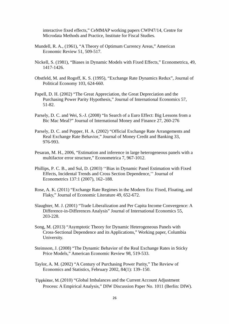
using the CCEP estimator with bias adjustments. The results from Table 6 reveal that

although the speed of current account (real exchange rate) adjustment is slower (faster)

for the euro period than for the pre-euro period, their difference is not significant at

conventional levels.26 These results agree with the results found by Chinn and Wei

(2013) and Ghosh et al. (2010) but differ qualitatively with those in Table 1 and

contrast with the predominant view that greater flexibility would be conducive to

these adjustments.

Third, we examine how the results in Table 1 are affected if cross-sectional

dependence of disturbances is not controlled and the bias of estimates is not adjusted. 26 The results for inflation rates are not reported since they are the same as those in Table 5.

17  

We therefore estimate (1)-(2) with the LSDV method without including

cross-sectional means. The results from Table 7 are similar to those in Table 1 for

current accounts and real exchange rates although the half-life estimates are generally

longer in Table 7. Inflation rate adjustment under the pre-euro period is faster instead

of slower than under the euro period although the difference is insignificant.

Finally, we examine how the results in Table 1 are affected if standard panel

data estimation methods are applied. Chinn and Wei (2013) and Ghosh et al. (2010,

2014) consider a dynamic panel model with a common intercept and a common set of

slope coefficients under each exchange rate regime. The standard POLS method is

applied to examine the effect of exchange rate regimes on current account adjustment.

We therefore postulate a common intercept, a common set of slope coefficients for all

individuals, and i.i.d. disturbances. This is equivalent to imposing the following

restrictions in (1)-(3): , ,n ni ca ca 1, 2, , 0n n n

i z i z i z , 0,z 0,n ni z , n=a, b,

, , .z ca q

The persistence of a variable is measured by the sum of its autoregressive

coefficients (Chinn and Wei, 2013; Ghosh et al., 2010, 2014). The hypothesis that the

persistence of current accounts for the pre-euro period is equal to that for the euro

period is examined by the F statistic. Only autoregressive coefficients are reported to

save space. The results from the left panel of Table 8 indicate that autoregressive

coefficients are all significant at the 5% level. The adjustment, measured by 1 minus

the sum of autoregressive coefficients, is slightly faster (slower) under the pre-euro

period than under the euro period for current accounts and real exchange rates

(inflation rates). Besides, real exchange rates are highly persistent in both regimes.

The sum of autoregressive coefficients under the pre-euro period is not significantly

different from that under the euro period for all variables.

Next, we relax the assumption of a common intercept but retain the assumption

of a common vector of slope coefficients for all individuals and of i.i.d. disturbances.

The resulting model is the standard fixed effects model and is estimated by LSDV.27

The results from the right panel of Table 8 are similar to those in the left panel.28

Although current account and real exchange rate adjustments are faster for the

27 We impose the following restrictions in (1)-(3): 1, 2, , 0n n n

i z i z i z , ,ca ,n ni ca n=a, b,

, , .z ca q 28 The models for current accounts, real exchange rates and inflation rates in Table 8 do not include a linear trend. This is the reason why only the results for inflation rates are the same as those in Table 3.

18  

pre-euro period than the euro period, the difference of the estimated adjustment before

and after the launch of the euro is not statistically significant for all three variables.

Applying the standard panel data estimation methods, we observe that current

accounts adjust faster under the pre-euro period than under the euro period although

the difference is not statistically significant. This finding differs from that in Ghosh et

al. (2014). The reason could be that Ghosh et al. (2014) use bilateral exchange rate

regimes and bilateral trade balances in their empirical analysis. In addition, the

irrelevance of the exchange rate regime to the adjustments of current accounts and

real exchange rates is observed, which is consistent with that for industrial countries

in Chinn and Wei (2013) and Ghosh (2010).

Three findings can be summarized from Tables 3-8. First, our finding that the

use of the euro is conducive to the adjustments of current accounts, real exchange

rates and inflation rates is not qualitatively affected if finite sample biases of estimates

are not corrected. Second, current accounts adjust faster for the pre-euro period than

for the euro period, although their difference is insignificant, when the model with a

constant intercept is applied, and when standard panel estimation methods are adopted.

Finally, the irrelevance of exchange rate regimes to the adjustments of current

accounts, real exchange rates and inflation rates tends to be observed when

contemporaneous dependence in disturbances is not controlled, when time-varying

smooth equilibrium of variables is not allowed, and when standard panel estimation

methods are applied.

6. Robustness

This section examines the robustness of the results in Table 1 with the years of

the currency, financial and energy crises being removed. Several different scenarios

are considered: shortening the sample period, removing the pre-ERM period

(1973Q2-1978Q4), changing the lag selection criteria, considering asymmetries

arising from the divergence of current account balances between the core and

periphery countries, and applying the difference-in-differences analysis. The lag

orders of the model are re-determined in each scenario based on the mean of the BIC

lags unless a specific lag selection criterion is clearly stated. The results for robustness

checks are not reported but they are available upon request from the authors.

First, we consider a shorter sample period that removes the years since the recent

global financial crisis (2008-2015). The estimated results are reported in Table A1,

19  

and they are similar to those in Table 1.29 In short, the adjustments of current

accounts, real exchange rates and inflation rates are slower in the pre-euro period

compared to the euro period. Second, the pre-euro period includes two exchange rates

regimes: the floating rate regime from 1973-1978 and the ERM regime from

1979-1998. It may not be appropriate to combine these two regimes into a single

regime. We therefore re-estimate the nested model with the sample period starting

from 1979. The empirical results reported in Table A2 are generally consistent with

those in Table 1.30

Third, we determine the optimal lag length by the median of the BICs, and the

results in Table A3 are not qualitatively different from those in Table 1. Fourth, the

Akaike information criterion (AIC) is applied to determine the lag length of the model

for each country, and the optimal lag length for each sub-period is determined by the

mean of the AICs. The results in Table A4 agree with those in Table 1.

Fifth, current account balances within the eurozone have been diverging since

1999. Figure 3 reports time series plots of current accounts for 11 European countries

after 1999. In a small group of countries, the periphery countries (mainly Italy, Spain,

Portugal, Ireland, and Greece), deficits become large and persistent, while another

group, the core countries (Austria, Belgium, Finland, France, Germany, and the

Netherland), registered large surpluses. To take into account this type of asymmetry in

current account adjustment, we start the empirical period from 1999 and estimate the

adjustment of current accounts for core and periphery countries. According to Figure

3, a core country’s current account over 1999-2011 generally appears to have a linear

trend. However, a periphery country’s current account appears to have nonlinear

smooth shifts in mean but without trend. We therefore apply the models with a linear

trend and with smooth shifts in the intercept, respectively, to estimate current account

adjustment for core and periphery countries. The years of financial crisis over

2008-2009 are removed in estimation.

The results from the first panel of Table A5 reveal that the half-life for core

29 We do not report the estimation results of current accounts in Table A1. This is because the sample period for current account ends at 2011Q4. Hence the results from removing 2008-2015 are the same as those from removing 2008-2011. 30 The significant enlargement and increasing integration of European communities between 1980 and 1993 lead to the creation of the European Union in 1993. Furthermore, the Maastricht Treaty, agreed to in 1991 and entered into force in 1993, placed an inflation convergence criterion for eurozone countries to achieve price stability within the zone. These could explain why inflation persistence in the ERM period is not significantly different from that in the euro period.

20  

countries is mildly larger than that for periphery countries when the model with

smooth shifts in the intercept is applied. Hence, the core-periphery effects do not have

a significant impact on current account adjustment. Similar results are obtained when

the model with a linear trend is applied as indicated in the second panel of Table A5.

Chinn and Wei (2013) examine the asymmetric effect of the sign of current accounts

on current account adjustment and find the adjustment of current account surpluses is

slower than that of current account deficits, but no statistically significant adjustment

differential is observed. Ghosh et al. (2010) find that the speed of current account

adjustment decreases when it is in deficits. Both papers adopt the model without trend.

Our results from the first panel of Table A5 are consistent with those in Ghosh et al.

(2010).

Sixth, to mitigate the concern that the paper’s findings are attributable, not to the

euro launch, but to broader and more global changes in monetary conditions, we

adopt a difference-in-differences (DID) analysis. Given the selected lag order of 2 for

both periods, the standard DID equation based on Slaughter (2001) is specified as

follows:

, 1 , 1 2 , 1 , 1 2 , 1 3 , 1

11 , 1 21 , 1 31 , 1 , ,

j j j j j jri t ri t ri t k ri t r ri t j ri t rj

j j j jri t r ri t j ri t rj ri t

z z z z d z d z d

z d z d z d

(4)

where , iti tz ca , , it itq is a filtered variable in which the regime-specific nonlinear

smoothing mean and trend are filtered out. The subscript r indicates the exchange rate

regime with r=0 for the flexible rate regime before 1999 and r=1 for the euro regime

after 1998. rd is the regime dummy variable, and it is equal to one if r=1 and zero

otherwise. The superscript j indicates the country group with j=0 for the control group

(non-eurozone countries) and j=1 for the treatment group (eurozone countries). jd is

the group dummy variable, and it is one if j=1 and zero otherwise. rjd is the

interaction of dummy variables, and it is one if 1r jd d and zero otherwise.31

The difference in persistence estimates between the pre-euro and euro periods is

31 The treatment group includes 8 eurozone countries for current accounts, 9 countries for real exchange rates (Germany is excluded but Belgium and Ireland are included), and 10 countries for inflation rates (Germany is included). The control group includes 9 countries having flexible exchange rates after 1998: Australia, Canada, Denmark, Japan, Norway, Sweden, Switzerland, the United Kingdom, and the United States for current accounts and real exchange rates. The control group for inflation rates includes 10 countries (Korea is included). Therefore, the numbers of countries in the treatment and control groups are also comparable.

21  

1 within the control group and 1 3 within the treatment group. Thus the

difference in differences is given by 3 = [( 1 3 ) - 1 ]. If the launch of the euro

speeds up the adjustment of current accounts among the eurozone countries, then 3

is significantly negative. The sample period starts from 1985 for current accounts and

from 1983 for real exchange rates and inflation rates in order to have comparable

observations before and after the euro period.

The results from the second column of Table A6 indicate that 1 is

insignificantly negative, but 1 3 and 3 are significantly negative for the case

of current accounts. These results indicate that the difference of current account

adjustment between the pre-euro and euro periods is insignificant for the control

group but is significant for the treatment group, which echoes our results in Tables 1

and 2. Furthermore, the significance of 3 supports that the adoption of the euro

significantly facilitates current account adjustment. As for real exchange rates, the use

of the euro does not significantly facilitate real exchange rate adjustment since 3 is

not significantly negative. The last column of Table A6 indicates that 1 is

significantly positive, 1 3 is insignificantly negative, and 3 is significantly

negative when inflation rates are applied.32 Again, the adoption of the euro quickens

the adjustment of inflation rates. In sum, the results from the DID estimation

generally echo our findings in Table 1, which oppose the Friedman hypothesis.

7. Conclusions

Are currency unions unduly inhibit the efficient adjustment of current accounts?

If nominal exchange rates provide a useful adjustment mechanism internationally,

current account adjustment should be faster for a flexible exchange-rate regime than

for a fixed-rate regime. Focusing on the event of the launch of the euro in 1999, we

examine if it facilitates the current account adjustment of the eurozone. Our model

allows nonlinear smooth shifts in mean, and the empirical method controls for

cross-sectional dependence of disturbances and the finite-sample bias of estimates.

We find that the adoption of the euro facilitates rather than hinders the

adjustments of current accounts, real exchange rates and inflation rates, which are

32 The lag order of the model for inflation rates is 2 under the pre-euro period and 1 under the euro period for the eurozone countries. This leads to the difficulty of specifying an appropriate DID equation. Our specification in (4) assumes that the lag order is 2 for both periods. The results are not qualitatively affected if the lag order is assumed to be 1 for both periods.

22  

robust to different scenarios. The above results are not qualitatively affected even

when the finite sample bias of CCEP estimates is not corrected. However, current

accounts adjust faster for the pre-euro period than for the euro period although in a

statistically insignificant manner, when the model with a constant intercept is applied,

and when standard panel estimation methods are adopted. The independence of

exchange rate regimes to current account, real exchange rate and inflation rate

adjustments tends to be observed when contemporaneous dependence in disturbances

is not controlled, when time-varying smooth equilibrium of variables is not allowed,

and when standard panel estimation methods are adopted.

23  

References

Alogoskoufis, G. S. and Smith, R. (1991) “The Phillips Curve, the Persistence of Inflation, and the Lucas Critique: Evidence from Exchange-Rate Regimes,” American Economic Review, Vol. 81, pp. 1254–75.

Berger, H. and Nitch, V. (2014) “Wearing Corset, Losing Shape: The Euro’s Effect on

Trade Imbalances,” Journal of Policy Modeling 36, 136-155. Bergin, P., Glick, R.,Wu, J.-L. (2013) “The Micro–Macro Disconnect of Purchasing

Power Parity.” Review of Economics and Statistics 95, 798–812. ---- (2014) “Mussa Redux and Conditional PPP.” Journal of Monetary Economics 68,

101-114. ---- (2016) “Conditional PPP and Real Exchange Rate Convergence in the Euro Area,”

NBER working paper no. 21979. Berka, M., Devereux, M. B. and Engel, C. (2012) “Real Exchange Rate Adjustment in

and out of the Eurozone,” American Economic Review: Papers and Proceedings 102, 179-185.

Berka, M. and Devereux, M. B. (2011) “What determines European Real Exchange

Rates,” Working paper, University of British Columbia. Blanchard, O. and Giavazzi, F. (2002) “Current Account Deficits in the Euro Area:

The End of the Feldstein-Horioka Puzzle,” Brooking Papers on Economic Activity 2, 148-186.

Burdekin, R. C. K. and Siklos, P. L. (1999) “Exchange Rate Regimes and Shifts in

Inflation Persistence: Does Nothing Else Matter,” Journal of Money, Credit and Banking 31, 235-247.

Chen, R., Milesi-Ferretti, G. M. and Tressel, T. (2013) “External Imbalances in the

Eurozone,” Economic Policy 28, 101-142. Chinn, M. D. and H. Ito (2006) “What Matters for Financial Development? Capital

Controls, Institution and Interactions,” Journal of Development Economics 82, 163-192.

Chinn, M. D. and Prasad, E. S. (2000) “Medium-Term Determinants of Current

Accounts in Industrial and Developing Countries: An Empirical Exploration,” NBER Working Paper 7581.

Chinn, M. D. and Wei, S.-J. (2013) “A Faith-Based Initiative Meets the Evidence:

Does A Flexible Exchange Rate Regime Really Facilitate Current Account Adjustment?” Review of Economics and Statistics 95, 68-184.

Chinn, M. D. and Wei, S.-J. (2008) “A Faith-Based Initiative: Does A Flexible

Exchange Rate Regime Really Facilitate Current Account Adjustment?” NBER

24  

Working Paper No. 14420 Choi, H. and Mark, N. C. (2009) “Trending Current Accounts,” Working paper,

University of Notre Dame. Choi, H. and Mark, N. C. and Sul, D. (2008) “Endogenous Discounting, the World

Saving Glut and the U.S. Current Account,” Journal of International Economics 75, 30-53.

Christopoulos, D. K. and Leo´n-Ledesma, M. A. (2010a) “Current

Account Sustainability in the US: What Did We Really Know About It? ” Journal of International Money and Finance 29, 442-459.

---- (2010b) “Smooth Breaks and Non-linear Mean Reversion: Post-Bretton Woods

Real Exchange Rates,” Journal of International Money and Finance 29, 1076-1093.

Chudik, A. and Pesaran, M. H. (2015) “Common correlated effects estimation of

heterogeneous dynamic panel data models with weakly exogenous regressors,” Journal of Econometrics 188, 393-420.

Clarida, R. H. (ed.) (2007) G7 Current Account Imbalances: Sustainability and

Adjustment? Chicago: University Chicago Press. Clower, E. and Ito, H. (2011) “The Persistence and Determinants of Current Account

Balances: The Implications for Global Rebalancing,” Working paper, University of Washington.

Decressin, J. and Stavrev, E. (2009) “Current Accounts in a Currency Union,”IMF

Working paper. (No, 09/127) De Vos, I. and Everaert, G. (2016), “Bias-corrected Common Correlated Effects

Pooled estimation in homogeneous dynamic panels,” Working paper, Ghent University.

Dornbusch, R. (1976) “Expectations and Exchange Rate Dynamics” Journal of

Political Economy 84, 1161-1176. ------ (1982), “PPP Exchange Rate Rules and Macroeconomic Stability,” Journal of

Political Economy, Vol. 90, pp. 158-65. Enders, W. and Lee, J., (2012), “A Unit Root Test Using a Fourier Series to

Approximate Smooth Breaks”, Oxford Bulletin of Economics and Statistics 74, 574-599.

Engel, C. and Hamilton, J.D. (1990) “ Long Swings in the Dollar: Are They in the

Data and Do Markets Know It?” American Economic Review 80, 689-713. Everaert, G. and De Groote, T. (2016) “Common Correlated Effects Estimation of

Dynamic Panels with Cross-Sectional Dependence,” Econometric Review 35,

25  

428-463. Frenkel, J. A. and Mussa, M. L (1985) “Asset Markets, Exchange Rates, and the Bal-

ance of Payments,” in Handbook of International Economics, Volume 2. Ronald W. Jones and Peter B. Kenen, eds. New York: Elsevier, North- Holland, 679–747.

Friedman, M. (1953) “The Case for Flexible Exchange Rates,” in M. Friedman,

Essays in Positive Economics, The University of Chicago Press. 157–203. Ghosh, A. R., Qureshi, M. S., & Tsangarides, C. G. (2014) “Friedman Redux:

External Adjustment and Exchange rate Flexibility,” IMF Working Paper 146, International Monetary Fund.

---- (2013), “Is the exchange rate regime really irrelevant for external adjustment?”

Economics Letters 118, 104-109. Ghosh, R. A., Terrones, M. and Zettelmeyer, J. (2010) “Exchange Rate Regimes and

External Adjustment: New Answers to an Old Debate,” The new international monetary system: Essays in honor of Alexander Swoboda, C. Wyplosz, ed.

Glushenkova, M. and Zachariadis, M. 2016. Understanding Law-Of-One-Price

Deviations Across Europe Before and After the Euro, forthcoming in the Journal of Money, Credit and Banking.

Herrmann, S. (2009) “Do We Really Know that Flexible Exchange Rates Facilitate

Current Account Adjustment? Some New Empirical Evidence for CEE Countries,” Applied Economics Quarterly 55, 295-312.

Huang, C.-H. and Yang, C.-Y. (2015) “European Exchange Rates and Purchasing

Power parity: An Empirical Study on Eleven Eurozone Countries,” International Review of Economics and Finance 35, 100-109.

Ju, J. and Wei, S.-J. (2007) “Current Account Adjustment: Some New Theory and

Evidence,” NBER Working Paper. (N. 13388). Kilian, L. (1998) ‘‘Small-Sample Confidence Intervals for Impulse Response

Functions,’’Review of Economics and Statistics 80, 218–230. Lane, P., Maria, and Milesi-Ferreti, G. M. (1999) “The External Wealth of Nations:

Measures of Foreign Assetsand Liabilities for Industrial and Developing Countries,” IMF working paper 99/115.

Leybourne, S., Mizen, P. (1999) “Understanding the Disinflations in Australia,

Canada and New Zealand Using Evidence from Smooth Transition Analysis,” Journal of International Money and Finance 18, 799–816.

Mann, C. (2002) “Perspectives on the U.S. Current Account Deficit and

Sustainability,” Journal of Economic Perspectives 16, 131-152. Moon, H. R. and Weidner, M. (2014) “Dynamic linear panel regression models with

26  

interactive fixed effects,” CeMMAP working papers CWP47/14, Centre for Microdata Methods and Practice, Institute for Fiscal Studies.

Mundell, R. A., (1961), “A Theory of Optimum Currency Areas,” American

Economic Review 51, 509-517. Nickell, S. (1981), “Biases in Dynamic Models with Fixed Effects,” Econometrica, 49,

1417-1426. Obstfeld, M. and Rogoff, K. S. (1995), “Exchange Rate Dynamics Redux”, Journal of

Political Economy 103, 624-660. Papell, D. H. (2002) “The Great Appreciation, the Great Depreciation and the

Purchasing Power Parity Hypothesis,” Journal of International Economics 57, 51-82.

Parsely, D. C. and Wei, S.-J. (2008) “In Search of a Euro Effect: Big Lessons from a

Bic Mac Meal?” Journal of International Money and Finance 27, 260-276 Parsely, D. C. and Popper, H. A. (2002) “Official Exchange Rate Arrangements and

Real Exchange Rate Behavior,” Journal of Money Credit and Banking 33, 976-993.

Pesaran, M. H., 2006, “Estimation and inference in large heterogeneous panels with a

multifactor error structure,” Econometrica 7, 967-1012. Phillips, P. C. B., and Sul, D. (2003) ‘‘Bias in Dynamic Panel Estimation with Fixed

Effects, Incidental Trends and Cross Section Dependence,’’ Journal of Econometrics 137:1 (2007), 162–188.

Rose, A. K. (2011) “Exchange Rate Regimes in the Modern Era: Fixed, Floating, and

Flaky,” Journal of Economic Literature 49, 652-672. Slaughter, M. J. (2001) “Trade Liberalization and Per Capita Income Convergence: A

Difference-in-Differences Analysis” Journal of International Economics 55, 203-228.

Song, M. (2013) “Asymptotic Theory for Dynamic Heterogeneous Panels with

Cross-Sectional Dependence and its Applications,” Working paper, Columbia University.

Steinsson, J. (2008) “The Dynamic Behavior of the Real Exchange Rates in Sticky

Price Models,” American Economic Review 98, 519-533. Taylor, A. M. (2002) “A Century of Purchasing Power Parity,” The Review of

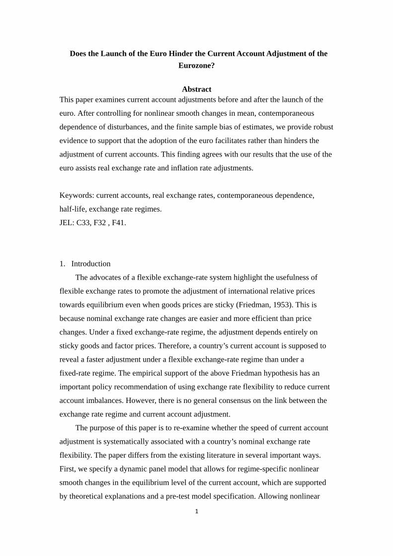
Economics and Statistics, February 2002, 84(1): 139–150. Tippkotter, M. (2010) “Global Imbalances and the Current Account Adjustment

Process: A Empirical Analysis,” DIW Discussion Paper No. 1011 (Berlin: DIW).

27  

Austria

-.6

-.4

-.2

.0

.2

.4

.6

1980 1985 1990 1995 2000 2005 2010

Finland

-1.5

-1.0

-0.5

0.0

0.5

1.0

1.5

2.0

2.5

1980 1985 1990 1995 2000 2005 2010

France

-.6

-.4

-.2

.0

.2

.4

.6

1980 1985 1990 1995 2000 2005 2010

Germany

-3

-2

-1

0

1

2

3

4

1980 1985 1990 1995 2000 2005 2010

Italy

-6

-4

-2

0

2

4

6

1980 1985 1990 1995 2000 2005 2010

Netherland

-3

-2

-1

0

1

2

3

4

1980 1985 1990 1995 2000 2005 2010

Portugal

-.10

-.08

-.06

-.04

-.02

.00

.02

.04

.06

1980 1985 1990 1995 2000 2005 2010

Spain

-.06

-.04

-.02

.00

.02

.04

1980 1985 1990 1995 2000 2005 2010 Figure 1. Plots of the ratio of current account to gross domestic product.

28  

A. Current accounts Pre-euro period Euro period

B. Real exchange rates Pre-euro period Euro period

C. Inflation rates Pre-euro period Euro period

Figure 2. The impulse response functions of current accounts, real exchange rates and inflation rates. The broken and dotted lines are the 5%-95% confidence intervals constructed based on Kilian’s (1998) double bootstrap method through 2000 iterations.

‐0.4

‐0.2

0

0.2

0.4

0.6

0 5 10 15 20 25 30 35

‐0.4

‐0.2

0

0.2

0.4

0.6

0 5 10 15 20 25 30 35

0

0.01

0.02

0.03

0 5 10 15 20 25 30 35

0

0.01

0.02

0.03

0 5 10 15 20 25 30 35

0

0.5

1

1.5

1 6 11 16 21 26 31 36

0

0.5

1

1.5

1 6 11 16 21 26 31 36

29  

Panel A: Core countries

Austria Belgium Finland

France Germany Netherlands

Panel B: Periphery countries

Italy Portugal Spain

Greece Ireland

Figure 3: Plots of the ratio of current account to gross domestic product for core and

periphery countries since 1999

-.4

-.3

-.2

-.1

.0

.1

.2

.3

99 00 01 02 03 04 05 06 07 08 09 10 11

-8

-6

-4

-2

0

2

4

6

99 00 01 02 03 04 05 06 07 08 09 10 11-1.5

-1.0

-0.5

0.0

0.5

1.0

1.5

99 00 01 02 03 04 05 06 07 08 09 10 11

-.6

-.4

-.2

.0

.2

.4

.6

.8

99 00 01 02 03 04 05 06 07 08 09 10 11

-4

-3

-2

-1

0

1

2

3

99 00 01 02 03 04 05 06 07 08 09 10 11-4

-3

-2

-1

0

1

2

3

99 00 01 02 03 04 05 06 07 08 09 10 11

-.03

-.02

-.01

.00

.01

.02

.03

99 00 01 02 03 04 05 06 07 08 09 10 11-.04

-.03

-.02

-.01

.00

.01

.02

.03

99 00 01 02 03 04 05 06 07 08 09 10 11

-8

-6

-4

-2

0

2

4

6

8

99 00 01 02 03 04 05 06 07 08 09 10 11-6

-4

-2

0

2

4

6

99 00 01 02 03 04 05 06 07 08 09 10 11

30  

Table 1. Nested estimation without data over 1992-1993 and 2008-2011 1 2

,z , , ,z , , ,1 1

,p p

a a b bit at it i z it j z it j bt it i z it j z it j it z

j j

z d x z d x z

where ,z 0, 1, 2, ,sin(2 / ) cos(2 / )n n n n nit i z i n i n iz zz kt T kt T t , for n=a, b,

b aT T T ; = , , ;it it i t itz ca q 1, , , 1, , .i N t T

Pre-Euro Euro Diff

Current accounts ( =it itz ca )

1itca 0.325** [0.21, 0.44] -0.236** [-0.44, -0.03] 0.561** [0.33, 0.80]

2itca -0.058 [-0.18, 0.06] -0.079 [-0.27, 0.12] 0.021 [-0.20, 0.25]

HL 0.741 [0.63, 0.89] 0.405 [0.35, 0.48] 0.336** [0.20, 0.50]

Real exchange rates ( =it itz q ), , , 0a bi z i z .

1itq 1.019** [0.95, 1.09] 0.673** [0.52, 0.81] 0.346** [0.19, 0.51]

2itq -0.160** [-0.23, -0.09] -0.010 [-0.14, 0.12] -0.150* [-0.30, -0.00]

HL 4.972 [3.87, 6.67] 1.750 [1.14, 2.65] 3.222** [1.80, 5.01]

Inflation rates ( =it itz ), , , 0n ni z i z , n=a,b.

1t 0.892** [0.80, 0.99] 0.697** [0.61, 0.78] 0.194** [0.07, 0.32]

2t -0.097 [-0.19, 0.00] --- --- --- ---

HL 3.294 [2.49, 4.67] 1.936 [1.47, 2.78] 1.358* [0.17, 2.90] Notes: itca , itq and it are the ratio of current account to gross domestic product,

real exchange rate and inflation rate, respectively, for the ith country at time t. Pre-euro and Euro stand for the pre-euro and euro periods, and they are 1977Q1-1998Q4 and 1999Q1-2011Q4 for current accounts and are 1973Q2-1998Q4 and 1999Q1-2015Q1 for real exchange rates and inflation rates. The lag length of the model is determined by the mean of the BIC lags. Numbers in the table are bias-adjusted estimates using the common correlated effects pooled (CCEP) methodology of Pesaran (2006) with bias adjustments using Kilian’s (1998) double bootstrap method with 1000 iterations. The 5%-95% confidence bands of bias adjusted estimates are reported in brackets and are constructed by bootstrap through 2000 replications. atd is a dummy variable for the pre-euro period, and its value is

one in the pre-euro period and zero in the post-euro period. btd is a dummy variable

for the euro period, and its value is one for 21at T p and zero otherwise, in

which aT is the last date of the pre-euro period. HL denotes the half-life in quarters,

which is calculated from the simulated impulse response function based on bias-adjusted estimates. Diff denotes the difference of autoregressive coefficients and half-lives between subsamples. The model includes a linear trend and a control ( itx )

for current accounts, a linear trend but no control for real exchange rates, and no trend and control for inflation rates. Two additional years of energy crises (1973 and 1979Q3-1980Q2) are also removed when inflation rates are applied. “**” and “*” indicate significance at the 5% and 10% level, respectively.

31  

Table 2. Nested Estimation for the 5 non-eurozone countries without data over

1992-1993 and 2008-2009 1 2

,z , , ,z , , ,1 1

,p p

a a b bit at it i z it j z it j bt it i z it j z it j it z

j j

z d x z d x z

where ,z 0, 1, 2, ,sin(2 / ) cos(2 / )n n n n nit i z i n i n iz zz kt T kt T t , for n=a, b,

b aT T T ; = , , ;it it i t itz ca q 1, , , 1, , .i N t T

Pre-Euro Euro Diff

Current accounts ( =it itz ca )

1itca 0.251** [0.14, 0.37] 0.142 [-0.01, 0.29] 0.108 [-0.08, 0.31]

2itca 0.020 [-0.10, 0.14] --- --- --- ---

HL 0.667 [0.58, 0.80] 0.583 [0.49, 0.70] 0.084 [-0.06, 0.24]

Real exchange rates ( =it itz q ), , , 0a bi z i z

1itq 0.856** [0.80,0.91] 0.901** [0.82, 0.97] -0.045 [-0.13, 0.06]

HL 4.478 [3.07, 7.47] 6.665 [3.41, 19.12] -2.187 [-14.39, 2.17]

Inflation rates ( =it itz ), , , 0n ni z i z , n=a, b

1t 1.040** [0.93, 1.15] 0.761** [0.61, 0.92] 0.279** [0.08, 0.47]

2t -0.241** [-0.39, -0.08] -0.052 [-0.20, 0.10] -0.188 [-0.40, 0.03]

3t -0.021 [-0.13, 0.09] --- --- --- ---

HL 3.510 [2.78, 4.64] 2.161 [1.51, 3.47] 1.349 [-0.16, 2.67] Notes: the 5 non-eurozone countries are Denmark, Norway, Sweden, Switzerland and the United Kingdom. Numbers in the table are CCEP estimates with bias adjustments. The 5%-95% confidence bands of CCEP estimates are reported in brackets, which are constructed by bootstrap through 2000 replications. Two additional years of energy crises (1973 and 1979Q3-1980Q2) are also removed when inflation rates are applied. Others are the same as those in Table 1.

32  

Table 3: Nested estimation without controlling for the three key components in

methodology and without data over 1992-1993 and 2008-2011 1 2

,z , , ,z , , ,1 1

,p p

a a b bit at it i z it j z it j bt it i z it j z it j it z

j j

z d x z d x z

,z 0, ,n n nit i z i zt , b aT T T ; = , , ;it it i t itz ca q 1, , , 1, , .i N t T

Pre-Euro Euro Diff

Current accounts ( =it itz ca )

1itca 0.660** [0.54, 0.77] 0.132 [-0.03, 0.29] 0.528** [0.32, 0.72]

2itca 0.134* [0.01, 0.24] 0.124 [-0.05, 0.27] 0.009 [-0.18, 0.21]

HL 2.652 [1.65, 4.00] 0.576 [0.48, 0.71] 2.076** [1.07, 3.41]

Real exchange rates ( =it itz q ), , , 0a bi z i z .

1itq 1.079** [0.99, 1.17] 0.692** [0.60, 0.80] 0.387** [0.24, 0.52]

2itq -0.160** [-0.26, -0.07] 0.250** [0.14, 0.34] -0.410** [-0.55, -0.27]

HL 8.735 [5.60, 13.96] 9.496 [6.31, 14.47] -0.761 [-7.01, 5.42]

Inflation rates ( =it itz ), , , 0n ni z i z , n=a,b.

1t 1.102** [1.01, 1.19] 0.941** [0.90, 0.97] 0.161** [0.07, 0.26]

2t -0.151** [-0.24, -0.06] --- --- --- ---

HL 14.506 [8.51, 25.03] 11.44 [6.51, 20.39] 3.065 [-7.80, 14.84]Notes: Disturbances are assumed to be identically and independently distributed, and the intercept for each individual is assumed to be a regime-specific constant. Numbers in the table are least squares dummy variables estimates, and the 5%-95% confidence bands are reported in brackets constructed by bootstrap through 2000 replications. Two additional years of energy crises (1973 and 1979Q3-1980Q2) are also removed when inflation rates are applied. Others are the same as those in Table 1.

33  

Table 4. Nested estimation without bias adjustments of estimates and without data over 1992-1993 and 2008-2011

1 2

,z , , ,z , , ,1 1

,p p

a a b bit at it i z it j z it j bt it i z it j z it j it z

j j

z d x z d x z

where ,z 0, 1, 2, ,sin(2 / ) cos(2 / )n n n n nit i z i n i n iz zz kt T kt T t , for n=a, b,

b aT T T ; = , , ;it it i t itz ca q 1, , , 1, , .i N t T

Pre-Euro Euro Diff

Current accounts ( =it itz ca )

1itca 0.319** [0.19, 0.43] -0.225* [-0.42, -0.01] 0.543** [0.29, 0.76]

2itca -0.060 [-0.18, 0.06] -0.077 [-0.27, 0.12] 0.017 [-0.21, 0.24]

HL 0.734 [0.62, 0.87] 0.408 [0.35, 0.49] 0.326** [0.18, 0.47]

Real exchange rates ( =it itz q ), , , 0a bi z i z

1itq 1.006** [0.92, 1.07] 0.657** [0.49, 0.78] 0.348** [0.20, 0.51]

2itq -0.157** [-0.23, -0.08] -0.013 [-0.15, 0.11] -0.144 [-0.29, 0.01]

HL 4.654 [3.48, 5.61] 1.660 [0.99, 2.28] 2.994** [1.66, 4.16] Inflation rates ( =it itz ), , , 0n n

i z i z , n=a, b

1t 0.874** [0.76, 0.95] 0.678** [0.57, 0.74] 0.196** [0.07, 0.33]

2t -0.093 [-0.19, 0.01] --- --- --- ---

HL 3.040 [2.20, 3.92] 1.818 [1.29, 2.37] 1.222* [0.23, 2.37] Notes: Numbers in the table are CCEP estimates without correcting the bias of estimates. The 5%-95% confidence bands of CCEP estimates are reported in brackets, which are constructed by bootstrap through 2000 replications. Two additional years of energy crises (1973 and 1979Q3-1980Q2) are also removed when inflation rates are applied. Others are the same as those in Table 1.

34  

Table 5. Nested estimation without smooth shifts in mean and without data over

1992-1993 and 2008-2011 1 2

,z , , ,z , , ,1 1

,p p

a a b bit at it i z it j z it j bt it i z it j z it j it z

j j

z d x z d x z

where ,z 0, ,n n nit i z i zt , for n=a, b; b aT T T ; = , , ;it it i t itz ca q

1, , , 1, , .i N t T Pre-Euro Euro Diff

Current accounts ( =it itz ca )

1itca 0.447** [0.32, 0.57] 0.090 [-0.11, 0.31] 0.357** [0.11, 0.60]

2itca 0.049 [-0.08, 0.18] 0.170 [-0.04, 0.36] -0.121 [-0.34, 0.14]

HL 0.904 [0.74, 1.29] 0.550 [0.45, 0.73] 0.355** [0.11, 0.74]

Real exchange rates ( =it itz q ), , , 0a bi z i z

1itq 1.086** [1.01, 1.16] 0.826** [0.69, 0.96] 0.260** [0.11, 0.42]

2itq -0.170** [-0.24, -0.10] 0.058 [-0.06, 0.18] -0.227** [-0.37, -0.08]

HL 8.588 [6.06, 13.03] 5.403 [3.02, 11.73] 3.185 [-3.31, 7.98]

Inflation rates ( =it itz ), , , 0n ni z i z , n=a, b

1t 0.939** [0.84, 1.04] 0.822** [0.75, 0.89] 0.117 [-0.00, 0.24]

2t -0.076 [-0.17, 0.02] --- --- --- ---

HL 4.952 [3.44, 8.13] 3.560 [2.44, 5.90] 1.392 [-1.33, 4.66] Notes: Numbers in the table are CCEP estimates with bias adjustments. The 5%-95% confidence bands of CCEP estimates are reported in brackets, which are constructed by bootstrap through 2000 replications. Two additional years of energy crises (1973 and 1979Q3-1980Q2) are also removed when inflation rates are applied. Others are the same as those in Table 1.

35  

Table 6. Nested estimation with a constant mean and without data over 1992-1993 and

2008-2011 1 2

,z , , ,z , , ,1 1

,p p

a a b bit at it i z it j z it j bt it i z it j z it j it z

j j

z d x z d x z

where ,z 0,n nit i z , for n=a, b; b aT T T ; = , , ;it it i t itz ca q

1, , , 1, , .i N t T Pre-Euro Euro Diff

Current accounts ( =it itz ca )

1itca 0.479** [0.35, 0.60] 0.369** [0.18, 0.57] 0.110 [-0.12, 0.34]

2itca 0.086 [-0.04, 0.22] 0.430** [0.23, 0.60] -0.344** [-0.56,-0.10]

HL 0.960 [0.77, 1.52] 2.334 [0.66, 6.89] -1.374 [-5.89, 0.47]

Real exchange rates ( =it itz q ), , , 0a bi z i z

1itq 1.090** [1.00, 1.18] 0.730** [0.64, 0.85] 0.359** [0.21. 0.50]

2itq -0.160** [-0.25, -0.07] 0.210** [0.10, 0.30] -0.370** [-0.50, -0.22]

HL 10.159 [6.59,18.55] 9.695 [6.69, 15.93] 0.464 [-7.22, 9.21] Notes: Numbers in the table are CCEP estimates with bias adjustments. The 5%-95% confidence bands of CCEP estimates are reported in brackets, which are constructed by bootstrap through 2000 replications.. The 5%-95% confidence bands of CCEP estimates are reported in brackets, which are constructed by bootstrap through 2000 replications. Others are the same as those in Table 1.

36  

Table 7. Nested estimation with i.i.d. disturbances, without correcting the bias of estimate, and without data over 1992-1993 and 2008-2011

1 2

,z , , ,z , , ,1 1

,p p

a a b bit at it i z it j z it j bt it i z it j z it j it z

j j

z d x z d x z

where ,z 0, 1, 2, ,sin(2 / ) cos(2 / )n n n n nit i z i n i n iz zz kt T kt T t , for n=a, b,

b aT T T ; = , , ;it it i t itz ca q 1, , , 1, , .i N t T

Pre-Euro Euro Diff

Current accounts ( =it itz ca )

1itca 0.611** [0.49, 0.72] -0.111 [-0.27, 0.05] 0.722** [0.51, 0.92]

2itca 0.097 [-0.02, 0.21] -0.079 [-0.24, 0.07] 0.176 [-0.02, 0.37]

HL 1.792 [0.99, 2.63] 0.450 [0.39, 0.53] 1.342** [0.55, 2.18]

Real exchange rates ( =it itz q ), , , 0a bi z i z

1itq 1.025** [0.93, 1.12] 0.562** [0.45, 0.68] 0.464** [0.31, 0.61]

2itq -0.186** [-0.28, -0.09] 0.186** [0.07, 0.29] -0.372** [-0.22, -0.51]

HL 4.475 [3.26, 6.15] 2.013 [0.91, 2.75] 2.462** [1.07, 4.59]

Inflation rates ( =it itz ), , , 0n ni z i z , n=a, b

1t 1.064** [0.97, 1.15] 0.910 [0.85, 0.95] 0.153** [0.06, 0.26]

2t -0.167** [-0.26, -0.07] --- --- --- ---

HL 6.870 [4.69, 10.15] 7.384 [4.38, 12.62] -0.514 [-6.29, 3.74] Notes: Disturbances are assumed to be identically and independently distributed (i.i.d.). Numbers in the table are least squares dummy variables (LSDV) estimates. The 5%-95% confidence bands of LSDV estimates are reported in brackets, which are constructed by bootstrap through 2000 replications. Two additional years of energy crises (1973 and 1979Q3-1980Q2) are also removed when inflation rates are applied. Others are the same as those in Table 1.

37  

Table 8. Nested estimation with standard POLS and LSDV and without data over 1992-1993 and 2008-2011

1 2

0, , 0, , ,1 1

,p p

a a b bit at i z z it j z it j bt i z z it j z it j it z

j j

z d x z d x z

= , , it it it itz ca q i=1,…,N; t=1,…T.

Model A (POLS) Model B (LSDV) Pre-Euro Euro Pre-Euro Euro Current accounts ( =it itz ca )

1itca 0.704** (0.067) 0.475** (0.077) 0.690** (0.067) 0.440** (0.082)

2itca 0.164** (0.069) 0.416** (0.069) 0.153** (0.069) 0.416** (0.074)

0.867 0.891 0.843 0.856

F 0.15 [0.70] 0.03 [0.86] Real exchange rates ( =it itz q ), 0a b

z z

1itq 1.130** (0.049) 0.812** (0.047) 1.087** (0.046) 0.725** (0.059)

2itq -0.131** (0.049) 0.188** (0.047) -0.162** (0.049) 0.212** (0.056)

0.999 0.999 0.925 0.937

F 0.001 [0.91] 0.33 [0.57] Inflation rates ( =it itz ), 0a b

z z

1it 1.109** (0.056) 0.945** (0.027) 1.102** (0.057) 0.941** (0.025)

2it -0.145** (0.054) --- -0.151** (0.055) ---

0.964 0.945 0.951 0.941

F 0.40 [0.54] 0.11 [0.74] Notes: Model A is the model with a common intercept and a common set of slope coefficients: 0,z 0,

n ni z , n=a, b, , , .z ca q However, model B is the fixed effects

model with heterogeneous intercepts. Model A is estimated by pooled ordinary least squares (POLS) method, and model B is estimated by the standard least squares dummy variables (LSDV) method. The standard error of an estimate is reported in a parenthesis. indicates the sum of autoregressive coefficients. F is the F statistic testing the hypothesis that the sum of autoregressive coefficients for the pre-euro period is the same as that for the euro period ( PE E ). The p-value of the F statistic

is reported in a bracket. Two additional years of energy crises (1973 and 1979Q3-1980Q2) are also removed when inflation rates are applied. Others are the same as those in Table 1.

38  

Table Appendix for the paper “Does the Launch of the Euro Hinder the Current

Account Adjustment of the Eurozone?”

Table A1. Nested estimation without data over 1992-1993 and 2008-2015

Table A2. Nested estimation without data over 1973-1978, 1992-1993 and 2008-2011

Table A3. Nested estimation with the lag order being determined by the median of

BICs and without data over 1992-1993 and 2008-2011

Table A4. Nested estimation with the AIC criterion and without data over 1992-1993

and 2008-2011

Table A5. Nested estimation for current accounts for core and periphery countries

without data over 2008-2009

Table A6. Difference in differences estimation without data over 1992-1993 and

2008-2011

39  

Table A1. Nested estimation without data over 1992-1993 and 2008-2015 1 2

,z , , ,z , , ,1 1

,p p

a a b bit at it i z it j z it j bt it i z it j z it j it z

j j

z d x z d x z

where ,z 0, 1, 2, ,sin(2 / ) cos(2 / )n n n n nit i z i n i n iz zz kt T kt T t , for n=a, b,

b aT T T ; = , , ;it it i t itz ca q 1, , , 1, , .i N t T

Pre-Euro Euro Diff

Real exchange rates ( =it itz q ), , , 0a bi z i z

1itq 1.019** [0.95, 1.09] 0.417** [0.32, 0.51] 0.603** [0.49, 0.73]

2itq -0.162** [-0.24, -0.09] --- --- --- ---

HL 4.959 [3.86, 6.65] 0.857 [0.73, 1.03] 4.101** [2.96, 5.77]

Inflation rates ( =it itz ), , , 0n ni z i z , n=a, b

1t 0.890** [0.79, 0.99] 0.654** [0.55, 0.75] 0.236** [0.10, 0.38]

2t -0.094 [-0.19, 0.00] --- --- --- ---

HL 3.294 [2.48, 4.69] 1.678 [1.19, 2.45] 1.615** [0.54, 3.01] Notes: Numbers in the table are CCEP estimates with bias adjustments. The 5%-95% confidence bands of CCEP estimates are reported in brackets, which are constructed by bootstrap through 2000 replications. The 5%-95% confidence bands of CCEP estimates are reported in brackets, which are constructed by bootstrap through 2000 replications. The end of sample period for current accounts is 2011Q4, and hence removing 2008-2011 from the whole sample yields the same results as removing 2008-2015 from the whole sample. We therefore do not repeatedly report the estimation results of current accounts in Table 5. Two additional years of energy crises (1973 and 1979Q3-1980Q2) are also removed when inflation rates are applied. Others are the same as those in Table 1.

40  

Table A2. Nested estimation without data over 1973-1978, 1992-1993 and 2008-2011 1 2

,z , , ,z , , ,1 1

,p p

a a b bit at it i z it j z it j bt it i z it j z it j it z

j j

z d x z d x z

where ,z 0, 1, 2, ,sin(2 / ) cos(2 / )n n n n nit i z i n i n iz zz kt T kt T t , for n=a, b,

b aT T T ; = , , ;it it i t itz ca q 1, , , 1, , .i N t T

Pre-Euro Euro Diff Current accounts ( =it itz ca )

1itca 0.356** [0.22, 0.49] -0.238** [-0.44, -0.03] 0.593** [0.34, 0.83]

2itca -0.084 [-0.21, 0.06] -0.082 [-0.27, 0.11] -0.002 [-0.24, 0.23]

HL 0.776 [0.64, 0.98] 0.404 [0.35, 0.48] 0.372** [0.22, 0.59]

Real exchange rates ( =it itz q ), , , 0a bi z i z

1tq 0.798** [0.74, 0.85] 0.654** [0.50, 0.80] 0.144 [-0.01, 0.31]

2tq --- --- 0.011 [-0.13, 0.15] --- ---

HL 3.079 [2.31, 4.27] 1.713 [1.00, 2.70] 1.365* [0.15, 2.71] Inflation rates ( =it itz ), , , 0n n

i z i z , n=a, b

1t 0.891** [0.79, 0.99] 0.706** [0.61, 0.80] 0.185** [0.05, 0.32]

2t -0.129** [-0.23, -0.03] --- --- --- ---

HL 2.879 [2.24, 3.99] 1.990 [1.48, 3.05] 0.890 [-0.36, 2.13]

Notes: Numbers in the table are CCEP estimates with bias adjustments. The 5%-95% confidence bands of CCEP estimates are reported in brackets, which are constructed by bootstrap through 2000 replications. The 5%-95% confidence bands of CCEP estimates are reported in brackets, which are constructed by bootstrap through 2000 replications. Two additional years of energy crises (1973 and 1979Q3-1980Q2) are also removed when inflation rates are applied. Others are the same as those in Table 1.

41  

Table A3. Nested estimation with the lag order being determined by the median of BICs and without data over 1992-1993 and 2008-2011

1 2

,z , , ,z , , ,1 1

,p p

a a b bit at it i z it j z it j bt it i z it j z it j it z

j j

z d x z d x z

where ,z 0, 1, 2, ,sin(2 / ) cos(2 / )n n n n nit i z i n i n iz zz kt T kt T t , for n=a, b,

b aT T T ; = , , ;it it i t itz ca q 1, , , 1, , .i N t T

Pre-Euro Euro Diff

Current accounts ( =it itz ca )

1itca 0.326** [0.21, 0.44] -0.184 [-0.37, 0.01] 0.510** [0.28, 0.72]

2itca -0.058 [-0.18, 0.06] --- --- --- ---

HL 0.742 [0.63, 0.89] 0.422 [0.37, 0.51] 0.320** [0.18, 0.48]

Real exchange rates ( =it itz q ), , , 0a bi z i z

1itq 1.019** [0.95, 1.09] 0.654** [0.54, 0.75] 0.365** [0.24, 0.50]

2itq -0.160** [-0.23, -0.09] --- --- --- ---

HL 4.975 [3.88, 6.67] 1.678 [1.17, 2.47] 3.296** [1.95, 5.07]

Inflation rates ( =it itz ), , , 0n ni z i z , n=a, b

1t 0.892** [0.80, 0.99] 0.697** [0.61, 0.78] 0.194** [0.07, 0.32]

2t -0.097 [-0.19, 0.00] --- --- --- ---

HL 3.294 [2.49, 4.67] 1. 936 [1.47, 2.78] 1.358* [0.17, 2.90] Notes: The lag orders of the model for the pre-euro and euro periods are determined by the median of BICs. Numbers in the table are CCEP estimates with bias adjustments. The 5%-95% confidence bands of CCEP estimates are reported in brackets, which are constructed by bootstrap through 2000 replications. The 5%-95% confidence bands of CCEP estimates are reported in brackets, which are constructed by bootstrap through 2000 replications. Two additional years of energy crises (1973 and 1979Q3-1980Q2) are also removed when inflation rates are applied. Others are the same as those in Table 1.

42  

Table A4. Nested estimation with the AIC criterion and without data over 1992-1993

and 2008-2011 1 2

,z , , ,z , , ,1 1

,p p

a a b bit at it i z it j z it j bt it i z it j z it j it z

j j

z d x z d x z

where ,z 0, 1, 2, ,sin(2 / ) cos(2 / )n n n n nit i z i n i n iz zz kt T kt T t , for n=a, b,

b aT T T ; = , , ;it it i t itz ca q 1, , , 1, , .i N t T

Pre-Euro Euro Diff Current accounts ( =it itz ca )

1itca 0.336** [0.22, 0.46] -0.236* [-0.44, -0.03] 0.572** [0.33, 0.81]

2itca -0.075 [-0.20, 0.06] -0.080 [-0.28, 0.11] -0.006 [-0.22, 0.25]

3itca 0.092 [-0.03, 0.22] --- --- --- ---

HL 0.754 [0.64, 0.92] 0.405 [0.35, 0.49] 0.349** [0.21, 0.52]

Real exchange rates ( =it itz q ), , , 0a bi z i z

1itq 1.018** [0.94, 1.10] 0.773** [0.62, 0.92] 0.245** [0.08, 0.41]

2itq -0.149** [-0.26, -0.04] 0.090 [-0.09, 0.25] -0.239** [-0.43, -0.03]

3itq -0.015 [-0.09, 0.06] -0.285** [-0.40, -0.16] 0.269** [0.13, 0.40]

HL 4.902 [3.82, 6.65] 2.506 [2.05, 3.13] 2.396** [1.17, 4.15]

Inflation rates ( =it itz ), , , 0n ni z i z , n=a, b

1t 0.883** [0.79, 0.99] 0.820** [0.70, 0.94] 0.063 [-0.09, 0.22]

2t 0.056 [-0.08, 0.18] -0.177** [-0.29, -0.06] 0.233** [0.05, 0.40]

3t -0.180** [-0.29, -0.08] --- --- --- ---

HL 3.587 [2.85, 4.59] 1.987 [1.60, 2.61] 1.599** [0.60, 2.60]

Notes: The optimal lag length is determined by the mean of AICs. Numbers in the table are CCEP estimates with bias adjustments. The 5%-95% confidence bands of CCEP estimates are reported in brackets, which are constructed by bootstrap through 2000 replications. The 5%-95% confidence bands of CCEP estimates are reported in brackets, which are constructed by bootstrap through 2000 replications. Two additional years of energy crises (1973 and 1979Q3-1980Q2) are also removed when inflation rates are applied. Others are the same as those in Table 1.

43  

Table A5. Nested estimation for current accounts for core and periphery countries without data over 2008-2009

, , , ,1

,p

it it ca i ca it j ca it j it caj

ca x ca

where , 0, 1, 2, ,sin(2 / ) cos(2 / )it ca i ca i ca i ca n i cakt T kt T t ,

1, , , 1, , .i N t T

Core countries Periphery Countries The model with nonlinear smooth shits in mean, , 0i ca .

1itca 0.273** [0.07, 0.47] 0.122 [-0.06, 0.30]

2itca 0.070 [-0.13, 0.27] --- --- HL 0.687 [0.54, 0.96] 0.569 [0.47, 0.72] The model with a linear trend, 1, 2, 0i ca i ca .

1itca 0.239** [0.04, 0.43] 0.271** [0.06, 0.47]

2itca 0.056 [-0.13, 0.25] --- --- HL 0.657 [0.52, 0.88] 0.685 [0.53, 0.94] Notes: The core group includes six eurozone countries having a current account surplus for most of the time after 1999: Austria, Belgium, Finland, France, Germany, the Netherlands. The periphery Group includes 5 eurozone countries having a current account deficit for most of the time after 1999: Greece, Ireland, Italy, Portugal, Spain. Numbers in the table are CCEP estimates with bias adjustments. The 5%-95% confidence bands of CCEP estimates are reported in brackets, which are constructed by bootstrap through 2000 replications. The 5%-95% confidence bands of CCEP estimates are reported in brackets, which are constructed by bootstrap through 2000 replications. Others are the same as those in Table 1.

44  

Table A6. Difference in differences estimation without data over 1992-1993 and

2008-2011

, 1 , 1 2 , 1 , 1 2 , 1 3 , 1

11 , 1 21 , 1 31 , 1 , ,

j j j j j jri t ri t ri t k ri t r ri t j ri t rj

j j j jri t r ri t j ri t rj ri t

z z z z d z d z d

z d z d z d

z ca z q z ( , )T CN N (8,9) (9,9) (10,10)

1 -0.271** (0.090) -0.166** (0.027) -0.082* (0.050)

2 -0.114 (0.100) 0.324** (0.050) 0.621** (0.162)

1 -0.155 (0.118) 0.021 (0.054) 0.113** (0.051)

2 -0.261** (0.141) -0.027 (0.061) -0.032 (0.059)

3 -0.435** (0.206) -0.107 (0.124) -0.130* (0.076)

11 -0.036 (0.125) -0.150** (0.069) -0.351* (0.198)

21 0.076 (0.131) -0.086 (0.102) -0.325* (0.181)

31 0.122 (0.170) -0.233* (0.131) 0.126 (0.221)

F 12.21 [0.00] 0.59 [0.44] 0.09 [0.76] Notes: Numbers in parentheses (brackets) are standard errors (p-values). TN and

CN are the number of countries in the treatment and control groups. , iti tz ca , , it itq

is a filtered variable in which the regime-specific nonlinear smoothing mean and trend are filtered out. F is the F statistic testing the hypothesis that the sum of 1 and 3

is zero. To have comparable observations before and after the launch of the euro, the sample period is from 1985Q1 to 2011Q4 for current accounts and from 1983Q1 to 2015Q1 for real exchange rates. The years of currency and financial crises (1992-1993, 2008-2011) are removed. The treatment group includes 8 eurozone countries for current accounts, 9 countries for real exchange rates (Germany is excluded but Belgium and Ireland are included), and 10 countries for inflation rates (Germany is included). The control group includes 9 countries having flexible exchange rates after 1998 for current accounts and real exchange rates: Australia, Canada, Denmark, Japan, Norway, Sweden, Switzerland, the United Kingdom, and the United States. The control group for inflation rates includes 10 countries (Korea is included). Therefore, the numbers of countries in the treatment and control groups are also comparable. “**” and “*” indicate significance at the 5% and 10% level, respectively.