Embed Size (px)
Citation preview
RAFAEL SAULO MARQUES RIBEIRO
JOHN S. L. McCOMBIE
GILBERTO TADEU LIMA
WORKING PAPER SERIES Nº 2017-11
Department of Economics - FEA/USP
Does Real Exchange Rate Undervaluation Really Promote Economic Growth?
DEPARTMENT OF ECONOMICS, FEA-USP WORKING PAPER Nº 2017-11
Does Real Exchange Rate Undervaluation Really Promote Economic Growth?
Rafael Saulo Marques Ribeiro ([email protected])
John S. L. McCombie ([email protected])
Gilberto Tadeu Lima ([email protected])
JEL Codes: F43; F31; D63; O33.
Keywords: Exchange rate; growth; income distribution; technological capabilities.
Abstract:
This article seeks to reassess the empirical literature on real exchange rate misalignment and growth in light of the extensive discussion about the relationship between income distribution and growth in developing economies. We state that the relationship between changes in the real exchange rate and growth can be characterised by two conflicting partial effects, as follows: i) undervaluation stimulates technological change and knowledge spillovers, thus affecting positively output growth; ii) undervaluation raises income inequality and hence harms output growth. Though there are a vast number of empirical studies presenting robust evidence of a positive relationship between currency undervaluation and growth for developing economies, none has yet explicitly considered the potentially negative distributional effects of undervaluation on growth. Our empirical model adds to this literature by suggesting that, once both functional income distribution and the level of technological capabilities are explicitly taken into account, the direct impact of real exchange rate misalignment on growth becomes statistically non-significant for a sample of developing countries. Further, based on our results, we state that the real exchange rate only affects growth indirectly through its impacts on functional income distribution and technological innovation. Our estimates have shown that the indirect impact of undervaluation on growth in developing countries is negatively signed.
Does Real Exchange Rate Undervaluation Really Promote
Economic Growth?
Rafael S. M. Ribeiro
(corresponding author) Department of Land Economy, University of Cambridge, Cambridge, UK
John S. L. McCombie Department of Land Economy, University of Cambridge, Cambridge, UK
Gilberto Tadeu Lima Department of Economics, University of São Paulo, São Paulo, Brazil
Abstract: This article seeks to reassess the empirical literature on real exchange rate misalignment and growth in light of
the extensive discussion about the relationship between income distribution and growth in developing economies. We state
that the relationship between changes in the real exchange rate and growth can be characterised by two conflicting partial
effects, as follows: i) undervaluation stimulates technological change and knowledge spillovers, thus affecting positively
output growth; ii) undervaluation raises income inequality and hence harms output growth. Though there are a vast number
of empirical studies presenting robust evidence of a positive relationship between currency undervaluation and growth for
developing economies, none has yet explicitly considered the potentially negative distributional effects of undervaluation on
growth. Our empirical model adds to this literature by suggesting that, once both functional income distribution and the
level of technological capabilities are explicitly taken into account, the direct impact of real exchange rate misalignment on
growth becomes statistically non-significant for a sample of developing countries. Further, based on our results, we state
that the real exchange rate only affects growth indirectly through its impacts on functional income distribution and
technological innovation. Our estimates have shown that the indirect impact of undervaluation on growth in developing
countries is negatively signed.
Keywords: Exchange rate, growth, income distribution, technological capabilities.
JEL Codes: F43, F31, D63, O33.
July
2017
2
1 Introduction
The impact of the real exchange rate (RER) misalignments on growth has been extensively documented in
the empirical literature but no solid consensus has emerged yet. First, there are different concepts of ‘RER
misalignment’1. Second, the concept of ‘RER misalignment’ presupposes the concept of ‘equilibrium RER’,
which creates some disagreement since different authors sometimes use different sets of explanatory
variables to estimate the equilibrium RER. Third, the literature also presents different results stemming from
different econometric techniques used to estimate the models2. In spite of these technical issues, the majority
of the literature seems to suggest that there is a positive relationship between a more competitive currency
and growth in emerging markets (Bleaney and Greenaway, 2001; Cottani, Cavallo and Khan, 1990; Dollar,
1992; Gala, 2007; Gala and Libanio, 2010; Ghura and Grennes, 1993; Gluzmann, Levy-Yeyati and
Sturzenegger, 2012; Levy-Yeyati, Sturzenegger, and Gluzmann, 2013; Loayza, Fajnzylber, and Calderón,
2005; Razmi, Rapetti and Skott, 2012; Rodrik, 2008; Vaz and Baer, 2014). Some theoretical arguments are
used to support this empirical relationship. It is claimed that outward-oriented policies, expressed in terms of
a devalued currency, in East Asian countries encouraged foreign trade and propelled economic growth,
whereas inward-oriented policies employed in Latin America and Africa, associated with overvalued
currencies hampered the growth of these regions (Cottani, Cavallo and Khan, 1990; Dollar, 1992). It is also
stated that bad institutions and market failures affect disproportionately more the tradable sector than the
non-tradable sector, and hence a currency undervaluation, that is an increase in the relative price of
tradables, might work as a second-best mechanism on developing countries to correct this distortion,
promote desirable structural change, and increase growth (Rodrik, 2008). Gala and Libanio (2010), from a
Kaldorian perspective, argue that a competitive currency is good for growth because it boosts the industrial
sector of the economy, which is where the increasing-returns activities are predominantly located. Therefore,
currency undervaluation may spur growth through incentives to technological capabilities, capital
accumulation and information spillovers to other firms and industries in the economy. Gala (2007) and
Levy-Yeyati, Sturzenegger, and Gluzmann (2013) suggest that RER undervaluation increases profit margins
by reducing real wages, hence boosting savings, investments and output growth3. Lastly, Guzman, Ocampo
and Stiglitz (2017) argue that a stable and competitive RER may encourage economic diversification
towards activities with higher technological content in developing economies.
However, very few empirical studies in this literature have explored the underlying distributional effects
of undervalued currency on growth4. Currency undervaluation, by increasing the price in domestic currency
of imported intermediate inputs used in the production process or by raising the service in domestic currency
of the private external debt, feeds through into the domestic prices, thus causing an inflationary effect in the
1 According to the literature, the most commonly used methods to estimate the RER misalignment are: (i) the PPP-based
measure, which uses deviations of the actual RER with respect to the Purchasing Power Parity (PPP) in a benchmark year; (ii) the black market premium, which consists of calculating the difference between the black market and the official exchange rates; and (iii) the model-based measure, which is calculated as a deviation of the actual RER with respect to the equilibrium RER. 2 Early studies employed pooled Ordinary Least Squares and fixed-effects panel data, whereas Generalized Method of Moments
and panel cointegration have become more common very recently. 3 Nonetheless, it is worth noting that a more recent empirical literature offers a more nuanced notion about the RER-growth
nexus. By incorporating non-linearities in the baseline regressions, some studies suggest that overvaluation and undervaluation may impact differently on growth (Nouira and Sekkat, 2012; Schroder, 2013), and also that the level of the RER misalignment matters (Aguirre and Calderon, 2005; Couharde and Sallenave, 2013). 4 Gala (2007) and Levy-Yeyati, Sturzenegger, and Gluzmann (2013) do not test the robustness of their models to the inclusion of
any measure of income distribution as control variable. However, it is worth noting that the post-Keynesian theory of growth in open economies has largely documented the impact of the RER on growth via changes in functional income distribution (see Bhaduri and Marglin, 1990; Blecker, 1989; Lima and Porcile, 2012; Ribeiro, McCombie and Lima, 2016).
3
economy and so reduces the real wages. In addition, undervaluation also enhances the price competitiveness
of domestic goods in the foreign markets and hence allows capitalists to increase the profit margins set over
prime costs. In short, a reduction of real wages associated with a possible increase in the profit margins due
to currency undervaluation redistributes income from workers to capitalists. Ergo, the supporters of currency
undervaluation, by and large, are somehow in line with a long tradition in economics that can be traced back
to the classics, Marx, Kaldor and Robinson which claims that growth is mainly driven by capital
accumulation financed by saving. The redistribution of income from wages to profits increases aggregate
saving (since capitalists have a higher marginal propensity to save than workers) and hence spurs capital
accumulation and output growth.
Alternatively, another tradition in the growth literature drawing upon the works of Kalecki, Keynes and
Steindl argues that rising inequality may lead to economic stagnation. The rationale behind this argument is
that higher inequality reduces aggregate consumption since households in the lower end of the income
distribution have a higher propensity to consume than those at the top of the income distribution, which
results in low levels of aggregate sales, low expected profits and so discourages capital accumulation. While
the existing research suggests that RER undervaluation may boost technological progress and growth, it
remains largely silent regarding the fact that undervaluation also raises income inequality and thus may
adversely impact economic growth. A number of other transmission channels through which income
inequality can harm growth can also be pointed out. Sociopolitical instability: more unequal societies tend to
lead individuals to engage in rent-seeking activities or other manifestations such as violent protests and
assassinations (e.g. Alesina and Rodrik, 1994). Human capital investment with borrowing constraints: if
wealth is more equally distributed more individuals are able to invest in human capital (e.g. Perotti, 1996;
Castelló-Climent and Doménech, 2002). Education/fertility decisions: More equal societies have lower
fertility rates and higher rates of investment within each family to finance the education of each child (e.g.
Perotti, 1996). Endogenous fiscal policy: the more equal the society is, the lesser the demand for
redistribution of income and, consequently, the lower the taxation on private investments (e.g. Alesina and
Rodrik, 1994; Persson and Tabellini, 1994). Foellmi and Zweimüller (2006) also argue that, from a demand-
side approach, a greater income inequality may harm innovation by reducing the consumption of a poor
majority, which could otherwise form mass markets. A vast empirical literature has also documented the
effects of greater inequality on growth. Nonetheless, there are still a number of methodological challenges to
be dealt with. The early literature on the subject largely used OLS estimation method and found a negative
impact of inequality on growth (e.g. Alesina and Rodrik, 1994; Persson and Tabellini, 1994; Clarke, 1995;
Perotti, 1996). Subsequent works using fixed-effects and random-effects panel and 3SLS models found
either positive or non-significant coefficients (e.g. Li and Zou, 1998; Barro, 2000). However, more recent
studies estimate the models through GMM difference and system and find that greater inequality reduces
growth for the whole sample. These studies also show that the impact seems to be negative for poorer
countries and positive for richer countries (Castelló-Climent, 2010; Halter, Oechslin and Zweimüller, 2014;
Ostry, Berg and Tsangarides, 2014; OECD, 2015). There is also little available data on inequality; inequality
measures usually differ with respect to the time span, countries coverage and reference unit. Despite all these
issues, the majority of the empirical literature seems to support the idea that an increase in income inequality
tends to reduce growth rates in developing countries.
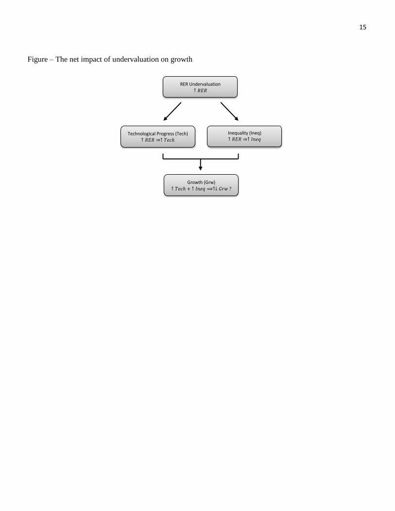
Motivated by these considerations, our paper seeks to contribute to the literature by reassessing the
undervaluation-growth nexus in light of the extensive research documenting the adverse impacts of greater
inequality on growth in emerging markets. As discussed above, the relationship between RER variations and
growth can be characterised by two conflicting partial effects, as follows: i) undervaluation stimulates
technological progress and knowledge spillovers, thus affecting positively output growth; and ii)
undervaluation raises income inequality by reducing real wages and hence harms aggregate consumption and
4
output growth. Ergo, the aim of this paper is to empirically verify the net impact of undervaluation on
growth.
[FIGURE ABOUT HERE]
We estimate two different cases: i) a baseline scenario in which growth depends on a set of conventional
explanatory variables including an index of RER misalignment; ii) a scenario of interest wherein growth is
regressed against the same set of explanatory variables (including the RER misalignment index) plus the
wage share in income and the relative level of technological capabilities of the country as control variables.
Unlike the previous studies, our findings suggest that by allowing for both the wage share and the relative
level of technological content of the country into the baseline growth equation the RER misalignment index
loses statistical significance indicating that relative prices have no direct impact on growth. Further empirical
tests have shown that a competitive currency may have an adverse, indirect impact on growth through
distributional effects and technological change.
In the next section we present very briefly the underlying theoretical framework of this article. In section
3 we discuss the data and methodology used in our estimates. In section 4 we test empirically our
hypotheses. Lastly, we conclude.
2 Technological progress, income distribution and growth: a brief overview
Now we must address the two key hypotheses of this work: i) the relationship between the level of
technological capabilities and growth; and ii) the impact of income distribution on output growth.
2.1 Technological progress, non-price competitiveness and growth
The first assumption is that in open economies an increase in the home country’s relative technological
capabilities spurs growth by improving its non-price competitiveness in foreign trade. This hypothesis is
strongly supported by the literature on theoretical and empirical grounds. Fagerberg (1988) questions the
traditional wisdom by suggesting that technology and the ability to compete on delivery are the main factors
affecting differences in international competitiveness, rather than relative unit labour costs reflecting
differences in price-competitiveness. He also finds evidence for 15 industrial countries during the period
1960-83 supporting his arguments. Amable and Verspagen (1995) find strong empirical evidence of the
positive impact of technological progress on exports market shares for 5 industrialised countries and 18
industries over the period 1970-91. Hughes (1986) proposes the hypothesis that there is a two-way
relationship between exports and innovation due to differences in the specificities of demand between export
and domestic markets in a study for 46 UK manufacturing industries. Léon-Ledesma (2002) extends also
finds a positive and statistically significant impact of technological innovations on exports and labour
productivity growth for 17 OECD countries from 1965-94. Araujo and Lima (2007) developed a
disaggregated multi-sectoral version of Thirlwall’s Law, where a country can reach higher growth rates only
by specialising in sectors with relatively high (low) income elasticities of demand for exports (imports).
Gouvea and Lima (2010) test the multi-sectoral model and their results, in general, support the hypothesis
that goods from relatively high technology-intensive sectors have higher (lower) income elasticities of
demand for exports (imports) and higher growth rates.
2.2 Income distribution and growth in open economies
As aforementioned, there are two traditions in the economic growth literature. On the one hand, we have the
classical-Marxian profit-led growth approach claiming that growth is mainly determined by saving and
5
capital accumulation. On the other hand, we have the Kaleckian-Steindlian wage-led growth tradition stating
that growth is driven by aggregate demand and capital accumulation (Dutt, 2017). Blecker (1989) and
Bhaduri and Marglin (1990) extend the demand-led growth approach in a more general formal framework
that accounts for both wage- and profit-led expansion patterns. In their model, if aggregate consumption is
more (less) responsive to an increase in the wage share than investment and net exports, then we have a
wage-led (profit-led) growth regime. According to this model, while a rising wage share boosts aggregate
consumption (due to the marginal propensity to consume differential), it reduces expected profitability and
harms price competitiveness of domestic goods in foreign trade and so adversely affects investment and net
exports. This is why many economists argue that it is less likely to observe a wage-led growth regime in
open economies.
However, there is a large body of theoretical and empirical works showing that rising wages may
stimulate labour-saving technological progress, capital deepening and so increase labour productivity (e.g.
Rowthorn, 1999; Storm and Naastepad, 2011; Vergeer and Kleinknecht, 2010-11). These results suggest that
the net effect of rising wages on relative unit labour cost and price competitiveness in open economies is an
empirical question. More recently, Blecker (2016) argues that demand is more likely to be profit led in the
short run and more likely to be wage led in the long run. Some empirical evidence support this conclusion by
showing that the effect of a rising wage share on aggregate demand is highly sensitive to lag lengths (Kiefer
and Rada, 2015; Vargas Sánchez and Luna, 2014).
In the context of open economies, variations in income distribution may also affect growth via changes in
the consumption pattern and, consequently, the country’s non-price competitiveness. International trade in
manufactured goods amongst developed countries can be heavily influenced by within-country income
levels and income inequality. Given the existence of non-homothetic preferences5, the more unequally
distributed the domestic income of a country, the greater its expenditures on luxury goods (Francois and
Kaplan, 1996). Latin American structuralists also claimed that high levels of income inequality in
developing countries led to sharp differences in the patterns of consumptions between the poor and the rich
within these countries. As the upper class in these countries used to imitate the pattern of consumption of
households from developed countries, a significant part of domestic saving leaked out of those countries in
order to maintain the imports of superfluous and highly technological products from developed countries,
thus slowing down investment and growth (Furtado 1968, 1969). A more recent literature also shows that,
given the non-homothetic preferences hypothesis, countries with higher levels of income inequality tend to
export more necessity goods and import more luxury goods (Mitra and Trindade, 2005; Bohman and
Nilsson, 2007; Dalgin, Trindade and Mitra, 2008; Lee and Hummels, 2017).
3 Methodology and data sources
3.1 The real exchange rate misalignment
To keep consistency and straight comparability with the literature, we draw on Rodrik (2008) to build an
undervaluation index. First of all, we take the data from the Penn World Tables for exchange rate (XRAT)
and PPP conversion factors (PPP) to calculate the log of the actual RER as follows:
ln(RER𝑖,𝑡) = ln(𝑋𝑅𝐴𝑇𝑖,𝑡 𝑃𝑃𝑃𝑖,𝑡⁄ ) (1)
5 Ernst Engel shows that consumers tend to substitute luxury (income elasticity of demand greater than unity) for necessity
(income elasticity of demand less than unity) goods, as income grows. Thus, the concept of non-homothetic preferences state that the share of income that consumers spend on luxury and necessity goods change as income increases.
6
The subscripts 𝑖 and 𝑡 account for country and time-period, respectively. The price of tradable goods is
usually given internationally, and the price of non-tradable goods is usually higher in developed countries.
This is the widely known Balassa-Samuelson effect and we must consider that in our index. To do so, we
must regress the log of the RER on the log of the GDP per capita (𝑞𝑖,𝑡):
ln(RER𝑖,𝑡̅̅ ̅̅ ̅̅ ̅̅ ) = 𝛾0 + 𝛾1𝑞𝑖,𝑡 + 𝑢𝑖,𝑡 (2)
Assuming the Balassa-Samuelson is statistically significant, we can specify the undervaluation index as
follows:
ln𝑈𝑁𝐷𝐸𝑅𝑉𝐴𝐿𝑖,𝑡 = ln(RER𝑖,𝑡) − ln(RER𝑖,𝑡̅̅ ̅̅ ̅̅ ̅̅ ) (3)
Our next step is to describe the growth equation in the light of our theoretical framework.
3.2 The growth equation
Here we seek to explain the growth performance of developing countries by using regression analysis. This
empirical analysis is based on a sample of several countries over several periods of time. We follow a well-
stablished empirical growth literature by describing a country’s growth rate as a function of economic
variables and then comparing the estimated model with the expected parameter values.
Most of the growth regressions in the literature follow the general specification below:
(𝑞𝑖,𝑡 − 𝑞𝑖,𝑡−1) 𝑛⁄ = 𝛽0 + 𝛽1𝑞𝑖,𝑡−1 + 𝛽2𝑆𝑖,𝑡 + 𝛽3𝜎𝑖,𝑡 + 𝛽4ln𝑈𝑁𝐷𝐸𝑅𝑉𝐴𝐿𝑖,𝑡 + 𝛽5𝑋𝑖,𝑡 + 𝜈𝑖 + 𝜅𝑡 + 𝜉𝑖,𝑡 (4)
where 𝛽0, 𝛽1, 𝛽2, 𝛽3, 𝛽4 and 𝛽5 are parameters (𝛽0 ≷ 0, 𝛽1 ≷ 0, 𝛽2 > 0, 𝛽3 > 0, 𝛽4 ≷ 0 and 𝛽5 ≷ 0 are the
expected signs), 𝑛 is the number of periods included, 𝑆 is the log of the relative level of technological
capabilities of each country, 𝜎 is the log of the wage share of income, 𝑋 is a set of control variables (all in
log), 𝜈 represent unobserved country-specific effect, 𝜅 is a period-specific effect, and 𝜉 is the regression
residual. The left-hand side of the equation above stands for the growth rate of the output per capita. On the
right-hand side, the equation includes the log of the initial output per capita to account for transitional
convergence, country- and time-specific effects, and a set of explanatory variables consisting of economic,
political and social variables according to the theoretical framework and the questions to be answered by the
model.
As discussed above, we can also say that both 𝑆𝑖,𝑡 and 𝜎𝐿𝑖,𝑡, in turn, depend on the currency
undervaluation index (𝑈𝑁𝐷𝐸𝑅𝑉𝐴𝐿𝑖,𝑡):
𝑆𝑖,𝑡 = 𝜁(ln𝑈𝑁𝐷𝐸𝑅𝑉𝐴𝐿𝑖,𝑡) + 𝜉𝑆𝑖,𝑡 (5)
𝜎𝐿𝑖,𝑡 = 𝜆(ln𝑈𝑁𝐷𝐸𝑅𝑉𝐴𝐿𝑖,𝑡) + 𝜉𝜎𝑖,𝑡 (6)
where 𝜁 and 𝜆 are parameters (𝜁 > 0 and 𝜆 < 0 are the expected signs), and 𝜉𝑆𝑖,𝑡 and 𝜉𝜎𝑖,𝑡 are the residuals
of equations (5) and (6) respectively. Once we have these equations, we can combine them all in order to
analyse and see the net impact of an undervaluation on long-run growth during a given time span as follows:
(𝑞𝑖,𝑡 − 𝑞𝑖,𝑡−1) 𝑛⁄ = 𝛽0 + 𝛽1𝑞𝑖,𝑡−1 + 𝛽∗ln𝑈𝑁𝐷𝐸𝑅𝑉𝐴𝐿𝑖,𝑡 + 𝛽5𝑋𝑖,𝑡 + 𝜈𝑖 + 𝜅𝑡 + 𝜉𝑖,𝑡
∗ (7)
7
where 𝛽∗ = 𝛽2𝜁 + 𝛽3𝜆 + 𝛽4 ≷ 0 and 𝜉𝑖,𝑡∗ = 𝜉𝑖,𝑡 + 𝛽2𝜉𝑆𝑖,𝑡 + 𝛽3𝜉𝜎𝑖,𝑡 are the extended parameter and residual
vectors, respectively. In our empirical study we intend to estimate the extended parameter 𝛽∗ = 𝛽2𝜁 + 𝛽3𝜆 +𝛽4. This extended parameter yields the indirect impact of undervaluation on growth of output per capita.
3.3 Database
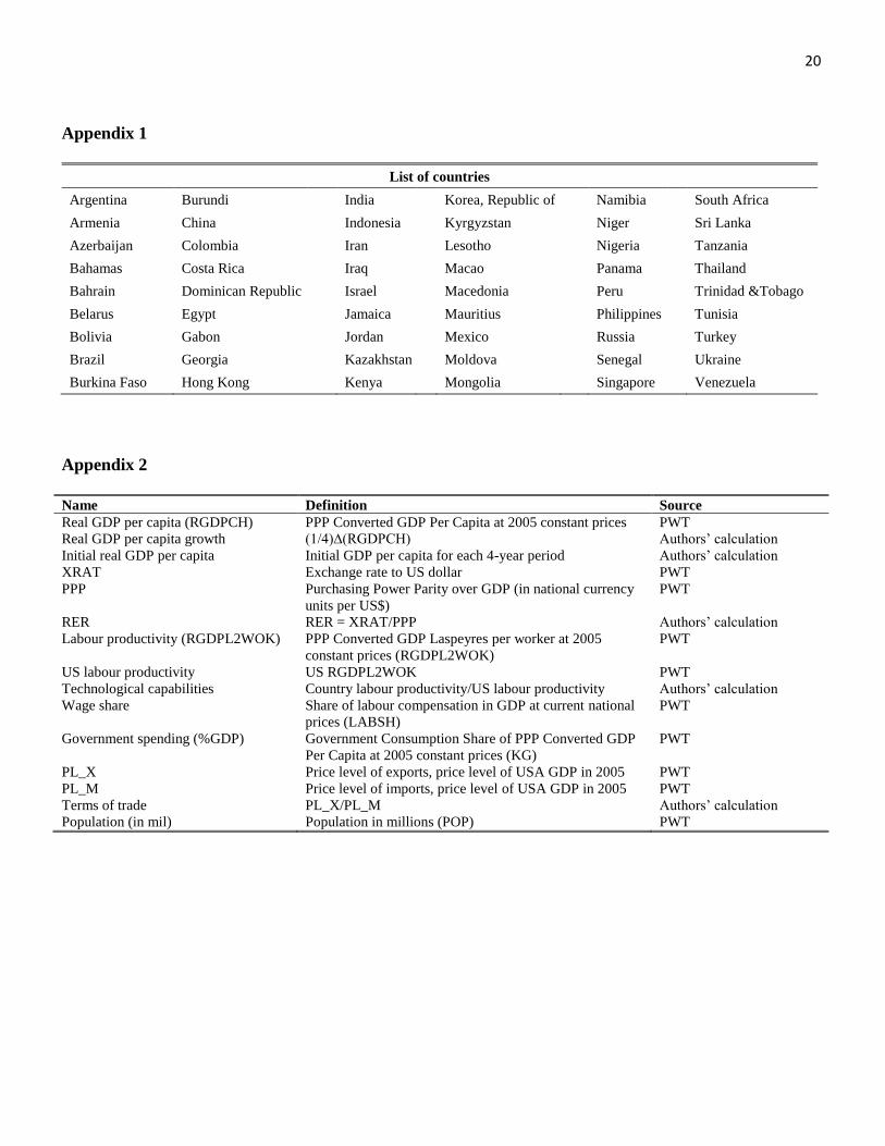
The sample consists of 54 developing countries and covers the period 1990-2010 (see the list of countries in
the Appendix 1 and the descriptions of the variables in the Appendix 2). Since in the literature a very weak
statistical relationship between a competitive currency and higher growth rates is usually observed for
developed countries (Gala, 2007; Rodrik, 2008), we decided to take into account only developing countries
in our sample. For the econometric estimates, all the variables were transformed into logarithms.
There are a large number of variables that can be used to explain growth. In order to maintain our work
consistent and comparable with the existing empirical literature, we have decided to take into account some
of the most commonly used variables in the previous studies.
The ‘initial real GDP per capita’ stands for the hypothesis of transitional dynamics. In mainstream growth
models, a country’s growth rate depends on the initial level of the GDP. The conditional convergence
hypothesis states that, other things held constant, economies that are lagging behind should grow faster than
the rich countries usually due to the existence of diminishing returns to factors of production. Even though
there is nothing in the Kaleckian-Steindlian theoretical approach that generates a tendency to convergence,
we nonetheless follow the existing literature and include the log of the initial GDP per capita as a potentially
explanatory variable in our regression.
Mainstream growth models also use ‘government spending (%GDP)’ as a proxy for government burden.
These models argue that governments can be a heavy burden on the economy when they impose high taxes,
promote inefficient programs, do not eliminate unnecessary bureaucracy, and distort market signals. The
proxy commonly used to account for the government burden is the ratio of government current expenditures
to GDP. However, mainstream economists, by and large, also acknowledge the importance of public
investments on health, education, and security to promote growth.
The ‘terms of trade’ and ‘period-specific dummy’ variables account for external factors that can affect
growth. Terms of trade tend to capture the external influence on each country, whereas the period-specific
dummies are used to capture external factors affecting all countries simultaneously. Terms of trade account
for changes in the foreign demand, relative costs of production, external financial inflows, etc. Period-
specific dummies capture worldwide conditions at a given period of time such as booms and recessions,
waves of technological change, economic reforms, etc.
The ‘population’ is included as an explanatory variable that accounts for the growth of the labour force.
The ‘technological capabilities’ variable is the ratio of each country’s labour productivity to the US
labour productivity. This is a proxy for 𝑆 from our growth equation (4), which is the relative technological
capability of the home country with respect to the foreign country. The rationale behind this proxy is based
on the assumption that countries with a higher level of technological capabilities also tend to have a higher
level of labour productivity. The US is used as a benchmark and represents the rich country pushing forward
the world technological frontier.
Here we use the ‘wage share’ as a measure of functional income distribution. In the analysis of wage-led
and profit-led growth regimes, income distribution is measured by the wage share of income. Inklaar and
Timmer (2013) show how the wage share displayed in the Penn World Tables is calculated.
8
3.4 Estimation method
In this subsection we outline the econometric technique used to estimate the growth equation. Here we use a
dynamic model of panel data. The growth regression presented above presents some challenges due to the
existence of unobserved time- and country-specific effects. Normally, we can solve this problem by allowing
into the baseline model period- and country-specific dummy variables. However, the methods used to
account for country-specific effects, that is, the fixed-effect or difference estimators, tend not to be
appropriate given the dynamic nature of the regression (Loayza, Fajnzylber and Calderón, 2005). Moreover,
most of the explanatory variables tend to be endogenous to the growth rate and hence simultaneity or reverse
causality must be properly controlled for.
In order to deal with these problems, we follow Arellano and Bond (1991), Arellano and Bover (1995)
and Blundell and Bond (1998), and use the Generalized Method of Moments (GMM) to estimate the
parameters of the model. These estimators are based on differencing regressions and instruments to control
for unobserved country-specific effects. Moreover, it also uses previous observations of dependent and
explanatory variables as instruments. There are two types of GMM estimation techniques: first-difference
GMM and the system GMM.
The GMM difference method represents a great improvement with respect to the standard fixed-effects
and first difference estimators. The first-difference GMM estimator by Arellano and Bond (1991) seeks to
eliminate country-specific effects and also uses lagged observations of the explanatory variables as
instruments. However, the first-difference GMM method has a disadvantage in dealing with variables that
tend to have a low degree of variability over time within a country, like income distribution for instance.
This implies that we eliminate most of the variation in the variable(s) by taking the first difference. In this
context, lagged observations of the explanatory variables tend to be weak instruments for the variables in
difference, thus yielding also weak estimators.
In order to solve this problem, we also use the system GMM by Arellano and Bover (1995) and Blundell
and Bond (1998). This method creates a system of regressions in difference and in level. The instruments of
the regressions in first difference remain the same as in the GMM difference. The instruments used in the
regressions in level are the lagged differences of the explanatory variables. Admittedly, in this estimation
technique, the explanatory variables can still be correlated with the country-specific effects; nevertheless, the
difference of these variables presents no correlation with these country-specific effects.
The validity of the GMM estimators depends greatly on the exogeneity of the instruments used in the
baseline model. The exogeneity of the instruments can be tested by the J statistics of the commonly used
Hansen test. The null hypothesis implies the joint validity of the instruments. In other words, a rejection of
the null hypothesis indicates that the instruments are not exogenous and hence the GMM estimator is not
consistent. Roodman (2009) advises researchers not to take comfort in a Hansen test p-value below 0.1. As
for the instruments, a large number of instruments is likely to overfit the endogenous variables. The
literature is not very specific in determining the maximum number of instruments to be used in each case.
Roodman (2009) suggests, as a relatively arbitrary rule of thumb, that instruments should not outnumber
individual units in the panel (or countries in our case). Here we tried to keep the number of instrumental
variables to a minimum and used up to 2 lags of the endogenous variables with the “collapse” function in
order to limit the proliferation of instruments.
The estimations were done using 4-year averages. This is a standard procedure in panel data analysis, as it
reduces the unwanted effects caused by unit roots. We have two types of variables: endogenous and
exogenous. The only exogenous variables in our model are ‘population’ and the period dummies.
9
4 Empirical assessment
To begin with, we estimate the relationship between RER and growth using the same procedure and similar
control variables employed in the literature (e.g. Gala, 2007; Rodrik, 2008). These results are reported in
Table 1. It can be seen that our finding is in accordance with the previous literature and also supports the
narrative that countries could spur growth by keeping the currency at competitive levels over long periods of
time.
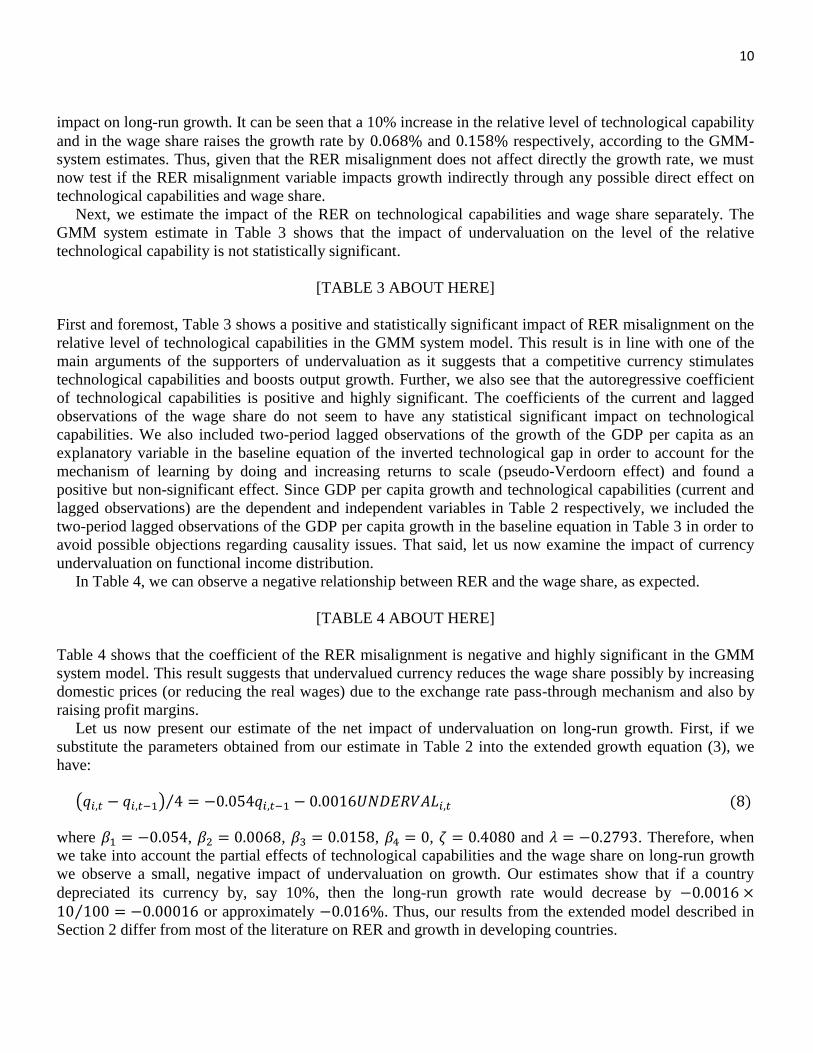
[TABLE 1 ABOUT HERE]
The first column shows the results of the pooled OLS estimator and the second column shows the results of
the fixed effects (within) OLS estimator. As previously mentioned, both methods are inconsistent. The third
and fourth columns present the results of the GMM difference and system, respectively. Our analysis will
focus on the estimates displayed in the fourth column, since the GMM-system is the preferred method of
estimation. As for the variable of interest, RER misalignment, we can see that its coefficient is positive and
statistically significant. A coefficient of 0.0142 means that if a country devalues its currency by 10%, then
the country growth rate increases by 0.0142x10/100 = 0.00142 or approximately 0.1%. This result is in
accordance with the previous studies cited above that estimate a linear relationship between RER
misalignment and growth6. Also note that the Hansen test does not reject the null hypothesis of non-
correlation between the instruments and the residuals.
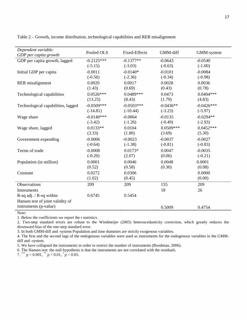
Nonetheless, when we include the level of technological capabilities and wage share in income as control
variables in the growth equation, we find very different results. Table 2 shows that when we allow for the
relative level of technological capabilities (current and lagged) and wage share (current and lagged) into the
baseline equation, the impact of RER misalignment on growth becomes statistically non-significant.
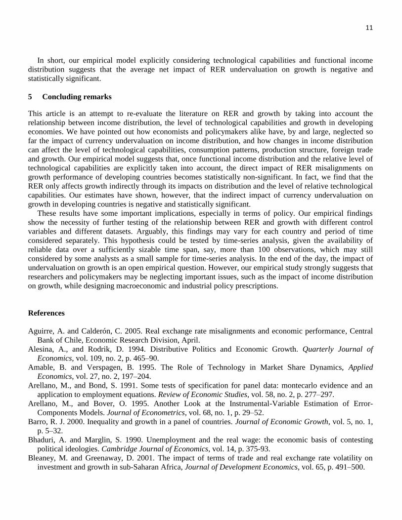
[TABLE 2 ABOUT HERE]
Table 2 shows that the coefficient of the autoregressive GDP per capita growth rate is negative, and
statistically significant. However, the most striking result of this estimation is that, once we control the GDP
per capita growth rate by the relative level of technological capabilities and wage share variables, the RER
misalignment coefficient becomes statistically non-significant.
Considering the GMM system estimates, the only statistically significant coefficients of the extended
growth equation are the coefficients of the technological capabilities and wage share variables. As for the
technological capabilities variable, the coefficient of the current impact of technological innovation on
growth is positive (0.0494), whereas the coefficient of the technological capabilities from the previous
period is negative -0.0426). This means that the overall impact of technological capabilities on growth is
0.0494 − 0.0426 = 0.0068. As for the wage share, we have also incorporated its current and the lagged
observations into the baseline equation. Table 2 shows that the current impact of the wage share on GDP per
capita growth is negative (-0.0294) and the lagged impact is positive (0.0452), thus yielding a positive
overall effect of an increased wage share on growth of −0.0294 + 0.0452 = 0.0158; therefore, our
empirical model is in accordance with the literature on growth and inequality and also shows that a more
evenly distributed income boosts growth.
Ergo, in the extended growth equation with technological capabilities and wage share the coefficient of
the RER misalignment loses its statistical significance. Moreover, if we consider the net impact of
technological capabilities and wage share on growth over time we find that both have a small, but significant
6 Rodrik and Gala estimates using GMM system found a coefficient of 0.015 and 0.0153 respectively.
10
impact on long-run growth. It can be seen that a 10% increase in the relative level of technological capability
and in the wage share raises the growth rate by 0.068% and 0.158% respectively, according to the GMM-
system estimates. Thus, given that the RER misalignment does not affect directly the growth rate, we must
now test if the RER misalignment variable impacts growth indirectly through any possible direct effect on
technological capabilities and wage share.
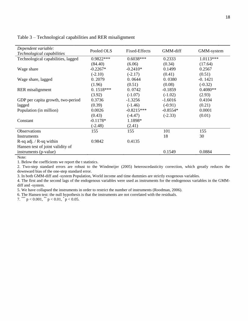
Next, we estimate the impact of the RER on technological capabilities and wage share separately. The
GMM system estimate in Table 3 shows that the impact of undervaluation on the level of the relative
technological capability is not statistically significant.
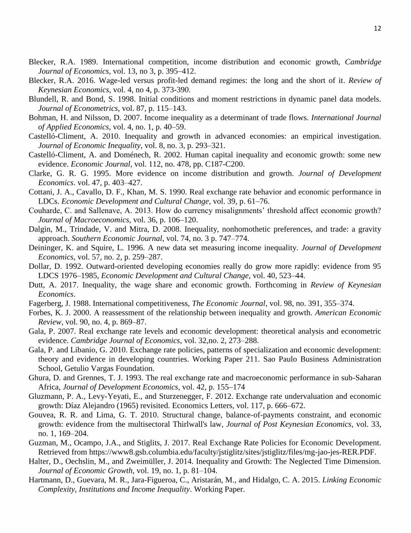
[TABLE 3 ABOUT HERE]
First and foremost, Table 3 shows a positive and statistically significant impact of RER misalignment on the
relative level of technological capabilities in the GMM system model. This result is in line with one of the
main arguments of the supporters of undervaluation as it suggests that a competitive currency stimulates
technological capabilities and boosts output growth. Further, we also see that the autoregressive coefficient
of technological capabilities is positive and highly significant. The coefficients of the current and lagged
observations of the wage share do not seem to have any statistical significant impact on technological
capabilities. We also included two-period lagged observations of the growth of the GDP per capita as an
explanatory variable in the baseline equation of the inverted technological gap in order to account for the
mechanism of learning by doing and increasing returns to scale (pseudo-Verdoorn effect) and found a
positive but non-significant effect. Since GDP per capita growth and technological capabilities (current and
lagged observations) are the dependent and independent variables in Table 2 respectively, we included the
two-period lagged observations of the GDP per capita growth in the baseline equation in Table 3 in order to
avoid possible objections regarding causality issues. That said, let us now examine the impact of currency
undervaluation on functional income distribution.
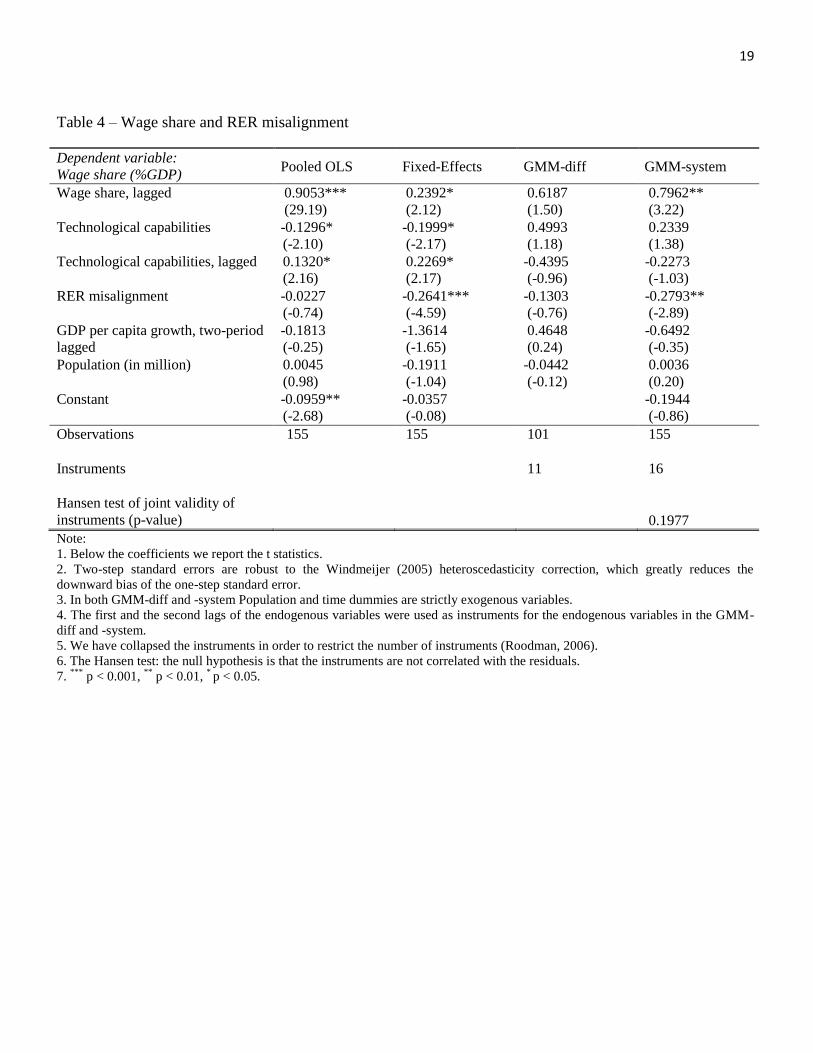
In Table 4, we can observe a negative relationship between RER and the wage share, as expected.
[TABLE 4 ABOUT HERE]
Table 4 shows that the coefficient of the RER misalignment is negative and highly significant in the GMM
system model. This result suggests that undervalued currency reduces the wage share possibly by increasing
domestic prices (or reducing the real wages) due to the exchange rate pass-through mechanism and also by
raising profit margins.
Let us now present our estimate of the net impact of undervaluation on long-run growth. First, if we
substitute the parameters obtained from our estimate in Table 2 into the extended growth equation (3), we
have:
(𝑞𝑖,𝑡 − 𝑞𝑖,𝑡−1) 4⁄ = −0.054𝑞𝑖,𝑡−1 − 0.0016𝑈𝑁𝐷𝐸𝑅𝑉𝐴𝐿𝑖,𝑡 (8)
where 𝛽1 = −0.054, 𝛽2 = 0.0068, 𝛽3 = 0.0158, 𝛽4 = 0, 𝜁 = 0.4080 and 𝜆 = −0.2793. Therefore, when
we take into account the partial effects of technological capabilities and the wage share on long-run growth
we observe a small, negative impact of undervaluation on growth. Our estimates show that if a country
depreciated its currency by, say 10%, then the long-run growth rate would decrease by −0.0016 ×10 100⁄ = −0.00016 or approximately −0.016%. Thus, our results from the extended model described in
Section 2 differ from most of the literature on RER and growth in developing countries.
11
In short, our empirical model explicitly considering technological capabilities and functional income
distribution suggests that the average net impact of RER undervaluation on growth is negative and
statistically significant.
5 Concluding remarks
This article is an attempt to re-evaluate the literature on RER and growth by taking into account the
relationship between income distribution, the level of technological capabilities and growth in developing
economies. We have pointed out how economists and policymakers alike have, by and large, neglected so
far the impact of currency undervaluation on income distribution, and how changes in income distribution
can affect the level of technological capabilities, consumption patterns, production structure, foreign trade
and growth. Our empirical model suggests that, once functional income distribution and the relative level of
technological capabilities are explicitly taken into account, the direct impact of RER misalignments on
growth performance of developing countries becomes statistically non-significant. In fact, we find that the
RER only affects growth indirectly through its impacts on distribution and the level of relative technological
capabilities. Our estimates have shown, however, that the indirect impact of currency undervaluation on
growth in developing countries is negative and statistically significant.
These results have some important implications, especially in terms of policy. Our empirical findings
show the necessity of further testing of the relationship between RER and growth with different control
variables and different datasets. Arguably, this findings may vary for each country and period of time
considered separately. This hypothesis could be tested by time-series analysis, given the availability of
reliable data over a sufficiently sizable time span, say, more than 100 observations, which may still
considered by some analysts as a small sample for time-series analysis. In the end of the day, the impact of
undervaluation on growth is an open empirical question. However, our empirical study strongly suggests that
researchers and policymakers may be neglecting important issues, such as the impact of income distribution
on growth, while designing macroeconomic and industrial policy prescriptions.
References
Aguirre, A. and Calderón, C. 2005. Real exchange rate misalignments and economic performance, Central
Bank of Chile, Economic Research Division, April.
Alesina, A., and Rodrik, D. 1994. Distributive Politics and Economic Growth. Quarterly Journal of
Economics, vol. 109, no. 2, p. 465–90.
Amable, B. and Verspagen, B. 1995. The Role of Technology in Market Share Dynamics, Applied
Economics, vol. 27, no. 2, 197–204.
Arellano, M., and Bond, S. 1991. Some tests of specification for panel data: montecarlo evidence and an
application to employment equations. Review of Economic Studies, vol. 58, no. 2, p. 277–297.
Arellano, M., and Bover, O. 1995. Another Look at the Instrumental-Variable Estimation of Error-
Components Models. Journal of Econometrics, vol. 68, no. 1, p. 29–52.
Barro, R. J. 2000. Inequality and growth in a panel of countries. Journal of Economic Growth, vol. 5, no. 1,
p. 5–32.
Bhaduri, A. and Marglin, S. 1990. Unemployment and the real wage: the economic basis of contesting
political ideologies. Cambridge Journal of Economics, vol. 14, p. 375-93.
Bleaney, M. and Greenaway, D. 2001. The impact of terms of trade and real exchange rate volatility on
investment and growth in sub-Saharan Africa, Journal of Development Economics, vol. 65, p. 491–500.
12
Blecker, R.A. 1989. International competition, income distribution and economic growth, Cambridge
Journal of Economics, vol. 13, no 3, p. 395–412.
Blecker, R.A. 2016. Wage-led versus profit-led demand regimes: the long and the short of it. Review of
Keynesian Economics, vol. 4, no 4, p. 373-390.
Blundell, R. and Bond, S. 1998. Initial conditions and moment restrictions in dynamic panel data models.
Journal of Econometrics, vol. 87, p. 115–143.
Bohman, H. and Nilsson, D. 2007. Income inequality as a determinant of trade flows. International Journal
of Applied Economics, vol. 4, no. 1, p. 40–59.
Castelló-Climent, A. 2010. Inequality and growth in advanced economies: an empirical investigation.
Journal of Economic Inequality, vol. 8, no. 3, p. 293–321.
Castelló-Climent, A. and Doménech, R. 2002. Human capital inequality and economic growth: some new
evidence. Economic Journal, vol. 112, no. 478, pp. C187-C200.
Clarke, G. R. G. 1995. More evidence on income distribution and growth. Journal of Development
Economics. vol. 47, p. 403–427.
Cottani, J. A., Cavallo, D. F., Khan, M. S. 1990. Real exchange rate behavior and economic performance in
LDCs. Economic Development and Cultural Change, vol. 39, p. 61–76.
Couharde, C. and Sallenave, A. 2013. How do currency misalignments’ threshold affect economic growth?
Journal of Macroeconomics, vol. 36, p. 106–120.
Dalgin, M., Trindade, V. and Mitra, D. 2008. Inequality, nonhomothetic preferences, and trade: a gravity
approach. Southern Economic Journal, vol. 74, no. 3 p. 747–774.
Deininger, K. and Squire, L. 1996. A new data set measuring income inequality. Journal of Development
Economics, vol. 57, no. 2, p. 259–287.
Dollar, D. 1992. Outward-oriented developing economies really do grow more rapidly: evidence from 95
LDCS 1976–1985, Economic Development and Cultural Change, vol. 40, 523–44.
Dutt, A. 2017. Inequality, the wage share and economic growth. Forthcoming in Review of Keynesian
Economics.
Fagerberg, J. 1988. International competitiveness, The Economic Journal, vol. 98, no. 391, 355–374.
Forbes, K. J. 2000. A reassessment of the relationship between inequality and growth. American Economic
Review, vol. 90, no. 4, p. 869–87.
Gala, P. 2007. Real exchange rate levels and economic development: theoretical analysis and econometric
evidence. Cambridge Journal of Economics, vol. 32,no. 2, 273–288.
Gala, P. and Libanio, G. 2010. Exchange rate policies, patterns of specialization and economic development:
theory and evidence in developing countries. Working Paper 211. Sao Paulo Business Administration
School, Getulio Vargas Foundation.
Ghura, D. and Grennes, T. J. 1993. The real exchange rate and macroeconomic performance in sub-Saharan
Africa, Journal of Development Economics, vol. 42, p. 155–174
Gluzmann, P. A., Levy-Yeyati, E., and Sturzenegger, F. 2012. Exchange rate undervaluation and economic
growth: Díaz Alejandro (1965) revisited. Economics Letters, vol. 117, p. 666–672.
Gouvea, R. R. and Lima, G. T. 2010. Structural change, balance-of-payments constraint, and economic
growth: evidence from the multisectoral Thirlwall's law, Journal of Post Keynesian Economics, vol. 33,
no. 1, 169–204.
Guzman, M., Ocampo, J.A., and Stiglits, J. 2017. Real Exchange Rate Policies for Economic Development.
Retrieved from https://www8.gsb.columbia.edu/faculty/jstiglitz/sites/jstiglitz/files/mg-jao-jes-RER.PDF.
Halter, D., Oechslin, M., and Zweimüller, J. 2014. Inequality and Growth: The Neglected Time Dimension.
Journal of Economic Growth, vol. 19, no. 1, p. 81–104.
Hartmann, D., Guevara, M. R., Jara-Figueroa, C., Aristarán, M., and Hidalgo, C. A. 2015. Linking Economic
Complexity, Institutions and Income Inequality. Working Paper.
13
Hughes, K. S. 1986. Exports and innovation: a simultaneous model, European Economic Review, vol. 30,
383–399.
Inklaar, R. and Timmer, M. P. 2013. Capital, labor and TFP in PWT8.0. Groningen Growth and
Development Centre, University of Groningen.
Kaldor, N. 1955. Alternative Theories of Distribution, Review of Economic Studies, Vol. 23, p. 83–100
Kiefer, D., and Rada, C. 2015. Profit maximising goes global: the race to the bottom, Cambridge Journal of
Economics, vol. 39, no. 5, p. 1333–50.
León-Ledesma, M. A. 2002. Accumulation, innovation and catching-up: an extended cumulative growth
model, Cambridge Journal of Economics, vol. 26, 201–216.
Levy-Yeyati, E., Sturzenegger, F., and Gluzmann, P. A. 2013. Fear of appreciation. Journal of Development
Economics, vol. 101, p. 233–247.
Lee, K.Y, and Hummels, D. 2017. The income elasticity of import demand: micro evidence and an
application. NBER Working Paper, no. 23338.
Li, H. and Zou, H. 1998. Income inequality is not harmful for growth: theory and evidence. Review of
Development Economics, vol. 2, no 3, p. 318–334.
Lima, G.T., and Porcile, G. 2013. Economic growth and income distribution with heterogeneous preferences
on the real exchange rate, Journal of Post Keynesian Economics, vol. 35, no. 4, p. 651–674.
Loayza, N., Fajnzylber, P., Calderón, C., 2005. Economic growth in Latin America and the Caribbean:
stylized facts, explanations, and forecasts. The World Bank Latin America and the Caribbean Regional
Studies Program, Washington, DC: The World Bank.
Matsuyama, K. 2000. Endogenous Inequality. The Review of Economic Studies, vol. 67, no. 4, p. 743–759
Mirrlees, J. 1971. An Exploration in the Theory of Optimum Income Taxation, Review of Economic Studies,
vol. 38, no. 114, p. 175–208.
Mitra, D. and Trindade, V. 2003. Inequality and trade, NBER Working Paper No. 10087.
Nouira, R. and Sekkat, K. 2012. Desperately seeking the positive impact of undervaluation on growth,
Journal of Macroeconomics, vol. 34, p. 537–552.
OECD. 2015. In It Together: Why Less Inequality Benefits All, OECD Publishing, Paris.
Ostry, J., Berg, A. and Tsangarides, C. 2014. Redistribution, Inequality, and Growth. IMF Staff Discussion
Note.
Perotti, R. 1996. Income distribution, and democracy: what the data say. Journal of Economic Growth, vol.
1, no. 2, p. 149–187.
Perraton, J. 2003. Balance-of-payments constrained economic growth and developing countries: an
examination of Thirlwall’s hypothesis. International Review of Applied Economics, vol. 17, no. 1, 1–22.
Persson, T., and Tabellini, G. 1994. Is inequality harmful for growth? The American Economic Review. vol.
84, no. 3, p. 600–621.
Razmi, A., Rapetti, M., and Skot, P. 2012. The real exchange rate and economic development, Structural
Change and Economic Dynamics, vol. 23, p. 151–169.
Ribeiro, R.S.M., McCombie, J.S.L., and Lima, G.T. 2016. Exchange rate, income distribution and technical
change in a balance-of-payments constrained growth model. Review of Political Economy, vol. 28, no. 4,
p. 545–565.
Rodrik, D. 2008. The real exchange rate and economic growth, Brookings Papers on Economic Activity, vol.
2008, no. 2, 365–412.
Roodman, D. 2009. How to do xtabond2: an introduction to difference and system GMM in Stata. The Stata
Journal, vol. 9, no. 1, p. 86–136.
Rosenzweig, M.R. and Binswanger, H. P. 1993. Wealth, weather risk and the composition and profitability
of agricultural investments. The Economic Journal, vol. 103, no. 416, p. 56–78.
14
Rowthorn, R.E. 1999. Unemployment, wage bargaining and capital-labour substitution. Cambridge Journal
of Economics, vol. 23, no 4, p. 413-425.
Schröder, M. 2013. Should developing countries undervalue their currencies? Journal of Development
Economics, vol. 105, p. 140–151.
Storm, S. and Naastepad, C.W.M. 2011. The productivity and investment effects of wage-led growth.
International Journal of Labour Research, vol. 3, no 2, p. 197-218.
Thirlwall, A.P. 1979. The balance of payments constraint as an explanation of international growth rate
differences. Banca Nazionale del Lavoro Quarterly Review, no. 128, March, 45–53.
Vargas Sánchez, G., and Luna, A. 2014. Slow growth in the Mexican economy, Journal of Post Keynesian
Economics, vol. 37, no. 1, p. 115–33.
Vaz, P. H. and Baer, W. 2014. Real exchange rate and manufacturing growth in Latin America. Latin
American Economic Review, vol. 23.
Vergeer, R. and Kleinknecht, A. 2010-11. The impact of labor market deregulation on productivity: a panel
data analysis of 19 OECD countries (1960-2004). Journal of Post Keynesian Economics, vol. 33, no 2, p.
369-405.
[APPENDIX 1 ABOUT HERE]
[APPENDIX 2 ABOUT HERE]
15
Figure – The net impact of undervaluation on growth
RER Undervaluation
Technological Progress (Tech)
Inequality (Ineq)
+ Growth (Grw)

16
Table 1 – Growth and RER misalignment
Dependent variable:
GDP per capita growth Pooled OLS Fixed-Effects GMM-diff GMM-system
GDP per capita growth, lagged 0.0923
(1.72)
-0.0044
(-0.07)
-0.0161
(-0.22)
0.0369
(0.43)
Initial GDP per capita -0.0005
(-0.88)
-0.0128**
(-2.65)
-0.0248
(-1.83)
-0.0011
(-0.56)
RER misalignment 0.0083***
(4.13)
0.0037
(1.10)
0.0021
(0.28)
0.0142**
(2.71)
Government spending -0.0022
(-1.46)
-0.0062**
(-2.65)
-0.0093*
(-2.38)
-0.0085*
(-2.18)
Terms of trade -0.0116
(-1.89)
0.0076
(0.64)
-0.0692
(-1.47)
-0.0456
(-1.39)
Population (in million) 0.0000
(0.12)
-0.0136
(-1.33)
-0.0112
(-0.56)
-0.0005
(-0.91)
Constant 0.0626*
(2.06)
0.1016
(1.36)
0.2227
(1.40)
Observations 209 209 155 209
Instruments 27 43
R-sq adj. / R-sq within 0.2556 0.0593
Hansen test of joint validity of
instruments (p-value)
0.0807 0.3024
Note:
1. Below the coefficients we report the t statistics.
2. Two-step standard errors are robust to the Windmeijer (2005) heteroscedasticity correction, which greatly reduces the
downward bias of the one-step standard error.
3. In both GMM-diff and -system Population and time dummies are strictly exogenous variables.
4. The first and the second lags of the endogenous variables were used as instruments for the endogenous variables in the GMM-
diff and -system.
5. We have collapsed the instruments in order to restrict the number of instruments (Roodman, 2006).
6. The Hansen test: the null hypothesis is that the instruments are not correlated with the residuals.
7. ***
p < 0.001, **
p < 0.01, * p < 0.05.
17
Table 2 – Growth, income distribution, technological capabilities and RER misalignment
Dependent variable:
GDP per capita growth Pooled OLS Fixed-Effects GMM-diff GMM-system
GDP per capita growth, lagged -0.2125***
(-5.15)
-0.1377**
(-3.03)
-0.0643
(-0.63)
-0.0540
(-1.00)
Initial GDP per capita -0.0011
(-0.56)
-0.0140*
(-2.36)
-0.0101
(-0.34)
-0.0084
(-0.98)
RER misalignment 0.0020
(1.43)
0.0017
(0.69)
0.0028
(0.43)
0.0036
(0.78)
Technological capabilities 0.0526***
(13.25)
0.0489***
(8.43)
0.0473
(1.79)
0.0494***
(4.83)
Technological capabilities, lagged -0.0509***
(-14.81)
-0.0503***
(-10.44)
-0.0436**
(-3.23)
-0.0426***
(-5.97)
Wage share -0.0140***
(-3.42)
-0.0064
(-1.26)
-0.0135
(-0.49)
-0.0294**
(-2.93)
Wage share, lagged 0.0133**
(3.33)
0.0104
(1.80)
0.0509***
(3.69)
0.0452***
(5.30)
Government expending -0.0006
(-0.64)
-0.0023
(-1.38)
-0.0037
(-0.81)
-0.0027
(-0.83)
Terms of trade -0.0008
(-0.20)
0.0173*
(2.07)
0.0047
(0.06)
-0.0035
(-0.21)
Population (in million) 0.0001
(0.52)
0.0046
(0.58)
0.0048
(0.30)
0.0001
(0.08)
Constant 0.0272
(1.02)
0.0306
(0.45)
0.0000
(0.00)
Observations 209 209 155 209
Instruments 18 26
R-sq adj. / R-sq within 0.6745 0.5454
Hansen test of joint validity of
instruments (p-value)
0.5009 0.4754
Note:
1. Below the coefficients we report the t statistics.
2. Two-step standard errors are robust to the Windmeijer (2005) heteroscedasticity correction, which greatly reduces the
downward bias of the one-step standard error.
3. In both GMM-diff and -system Population and time dummies are strictly exogenous variables.
4. The first and the second lags of the endogenous variables were used as instruments for the endogenous variables in the GMM-
diff and -system.
5. We have collapsed the instruments in order to restrict the number of instruments (Roodman, 2006).
6. The Hansen test: the null hypothesis is that the instruments are not correlated with the residuals.
7. ***
p < 0.001, **
p < 0.01, * p < 0.05.
18
Table 3 – Technological capabilities and RER misalignment
Dependent variable:
Technological capabilities Pooled OLS Fixed-Effects GMM-diff GMM-system
Technological capabilities, lagged 0.9822***
(84.40)
0.6038***
(6.06)
0.2333
(0.34)
1.0113***
(17.64)
Wage share -0.2267*
(-2.10)
-0.2410*
(-2.17)
0.1499
(0.41)
0.2567
(0.51)
Wage share, lagged 0. 2079
(1.96)
0. 0644
(0.51)
0. 0380
(0.08)
-0. 1421
(-0.32)
RER misalignment 0. 1518***
(3.92)
0. 0742
(-1.07)
-0.1859
(-1.02)
0.4080**
(2.93)
GDP per capita growth, two-period
lagged
0.3736
(0.39)
-1.3256
(-1.46)
-1.6016
(-0.91)
0.4104
(0.21)
Population (in million) 0.0026
(0.43)
-0.8215***
(-4.47)
-0.8554*
(-2.33)
0.0001
(0.01)
Constant -0.1178*
(-2.48)
1.1898*
(2.41)
Observations 155 155 101 155
Instruments 18 30
R-sq adj. / R-sq within 0.9842 0.4135
Hansen test of joint validity of
instruments (p-value)
0.1549 0.0884
Note:
1. Below the coefficients we report the t statistics.
2. Two-step standard errors are robust to the Windmeijer (2005) heteroscedasticity correction, which greatly reduces the
downward bias of the one-step standard error.
3. In both GMM-diff and -system Population, World income and time dummies are strictly exogenous variables.
4. The first and the second lags of the endogenous variables were used as instruments for the endogenous variables in the GMM-
diff and -system.
5. We have collapsed the instruments in order to restrict the number of instruments (Roodman, 2006).
6. The Hansen test: the null hypothesis is that the instruments are not correlated with the residuals.
7. ***
p < 0.001, **
p < 0.01, * p < 0.05.
19
Table 4 – Wage share and RER misalignment
Dependent variable:
Wage share (%GDP) Pooled OLS Fixed-Effects GMM-diff GMM-system
Wage share, lagged 0.9053***
(29.19)
0.2392*
(2.12)
0.6187
(1.50)
0.7962**
(3.22)
Technological capabilities -0.1296*
(-2.10)
-0.1999*
(-2.17)
0.4993
(1.18)
0.2339
(1.38)
Technological capabilities, lagged 0.1320*
(2.16)
0.2269*
(2.17)
-0.4395
(-0.96)
-0.2273
(-1.03)
RER misalignment -0.0227
(-0.74)
-0.2641***
(-4.59)
-0.1303
(-0.76)
-0.2793**
(-2.89)
GDP per capita growth, two-period
lagged
-0.1813
(-0.25)
-1.3614
(-1.65)
0.4648
(0.24)
-0.6492
(-0.35)
Population (in million) 0.0045
(0.98)
-0.1911
(-1.04)
-0.0442
(-0.12)
0.0036
(0.20)
Constant -0.0959**
(-2.68)
-0.0357
(-0.08)
-0.1944
(-0.86)
Observations 155 155 101 155
Instruments 11 16
Hansen test of joint validity of
instruments (p-value)
0.1977
Note:
1. Below the coefficients we report the t statistics.
2. Two-step standard errors are robust to the Windmeijer (2005) heteroscedasticity correction, which greatly reduces the
downward bias of the one-step standard error.
3. In both GMM-diff and -system Population and time dummies are strictly exogenous variables.
4. The first and the second lags of the endogenous variables were used as instruments for the endogenous variables in the GMM-
diff and -system.
5. We have collapsed the instruments in order to restrict the number of instruments (Roodman, 2006).
6. The Hansen test: the null hypothesis is that the instruments are not correlated with the residuals.
7. ***
p < 0.001, **
p < 0.01, * p < 0.05.
20
Appendix 1
List of countries
Argentina Burundi
India
Korea, Republic of Namibia
South Africa
Armenia
China
Indonesia Kyrgyzstan Niger
Sri Lanka
Azerbaijan Colombia
Iran
Lesotho
Nigeria
Tanzania
Bahamas
Costa Rica Iraq
Macao
Panama
Thailand
Bahrain
Dominican Republic Israel
Macedonia Peru
Trinidad &Tobago
Belarus
Egypt
Jamaica
Mauritius
Philippines Tunisia
Bolivia
Gabon
Jordan
Mexico
Russia
Turkey
Brazil
Georgia
Kazakhstan Moldova
Senegal
Ukraine
Burkina Faso Hong Kong Kenya
Mongolia
Singapore Venezuela
Appendix 2
Name Definition Source
Real GDP per capita (RGDPCH) PPP Converted GDP Per Capita at 2005 constant prices PWT
Real GDP per capita growth (1/4)∆(RGDPCH) Authors’ calculation
Initial real GDP per capita Initial GDP per capita for each 4-year period Authors’ calculation
XRAT Exchange rate to US dollar PWT
PPP Purchasing Power Parity over GDP (in national currency
units per US$)
PWT
RER RER = XRAT/PPP Authors’ calculation
Labour productivity (RGDPL2WOK) PPP Converted GDP Laspeyres per worker at 2005
constant prices (RGDPL2WOK)
PWT
US labour productivity US RGDPL2WOK PWT
Technological capabilities Country labour productivity/US labour productivity Authors’ calculation
Wage share Share of labour compensation in GDP at current national
prices (LABSH)
PWT
Government spending (%GDP) Government Consumption Share of PPP Converted GDP
Per Capita at 2005 constant prices (KG)
PWT
PL_X Price level of exports, price level of USA GDP in 2005 PWT
PL_M Price level of imports, price level of USA GDP in 2005 PWT
Terms of trade PL_X/PL_M Authors’ calculation
Population (in mil) Population in millions (POP) PWT