Embed Size (px)
Citation preview

200
.... Does investment cause growth? A test of an endogenous demand-driven theory of growth applied to India 1950-96
Ramesh Chandra and Roger J. Sandilands
…1. INTRODUCTION
From the early development literature of the 1940s and 1950s, notably that of Paul Rosenstein-Rodan (1943, 1961), Ragnar Nurkse (1953) and Arthur Lewis (1954), a mainstream view emerged that capital accumulation was the key to growth. Capital was the ‘missing component’ which if applied in adequate amounts could help break the vicious circle of poverty. Underdevelopment and low productivity were diagnosed as the result of an acute shortage of material capital, so the key to enhanced productivity lay in measures to boost the savings and investment rates.
For various reasons, there has been growing scepticism that physical capital is the main constraint on development. First, the neoclassical growth accounting exercises have found that increase in capital per worker explains only a small proportion of per capita income growth, a large portion of which is attributed to the unexplained residual or exogenous technical progress. Second, the new endogenous growth theory focuses on the externalities associated with new knowledge and emphasises the importance of human capital and research and development in offsetting the tendency to diminishing returns. Thus the above theories all tend to focus on supply constraints: physical or human capital, or the supply of new knowledge. The aim of the present paper is to offer and test a contrasting approach that is based on the demand side. Its essence can be summarised by reference to Adam Smith’s famous aphorism that the division of labour is limited by the size of the market, or Allyn Young’s extension of this theme – that the division of labour is limited by the division of labour.

Does investment cause growth? 201
The Indian five-year plans did not diverge from the early mainstream view on development issues. India’s development strategy since the second plan (1956–61) has come to be known as the Nehru-Mahalanobis strategy. This strategy accorded primacy to the capital goods sector and advocated a socialist framework in which the public sector would play a dominating role. In line with mainstream thinking, India’s planners subscribed to the supply-side view of the growth process in which capital accumulation was key (see, for example, Chakravarty, 1987). Given the added assumption of low elasticity of export demand (i.e., elasticity pessimism) and the need to convert high savings into real investment, primacy to capital goods production at home was thought to be the logical outcome.
As a result of policies derived from this thinking, India’s planners succeeded in pushing up the rates of saving and investment from around 10% in 1950 to around 22 percent by 1980; but there was no commensurate increase in the growth rate. Bhagwati (1993) stated that the weak growth performance reflected, not a disappointing saving performance, but rather a disappointing productivity performance.
Thus the theoretical, but also the empirical, question is: Is capital accumulation (or investment) really the main key to growth? The empirical literature seems divided on the issue. The observed strong relationship between fixed capital formation (as a percentage of GDP) and growth rates since World War II led DeLong and Summers (1991, 1992) to suggest that the rate of capital formation determines the rate of a country’s economic growth. Lipsey and Kravis (1987), on the other hand, find that the observed long-term relationship between the capital formation rate and the growth rate is due more to the effect of growth on capital formation than to the effect of capital formation on growth. In a recent paper Blomström et al. (1996) test the causality between the fixed investment rate and the growth rate by using the Granger (1969) and Sims (1972) framework. They find that economic growth precedes capital formation and that there is no evidence that capital formation precedes growth.
Given the importance attached to capital formation in India’s planning process and the evidence that the observed strong relationship between the fixed capital formation rate and the growth rate since World War II does not prove causality, the objective of this paper is to explore whether higher investment leads to higher growth in India. Our aim is to investigate which of the two contrasting approaches to development is supported by the Indian data: the capital accumulation approach which gives a causative role to capital accumulation, or the Smith–Young demand-based approach in which capital accumulation is more an effect than a cause of growth. Using data from the National Accounts Statistics, we investigate the issue of causality by using cointegration and error-correction modelling.

202 Old and New Growth Theories: an Assessment
The next section of this paper reviews in greater detail the nature of these contrasts. Methodological issues are discussed in Section ....3. Section ....4 then subjects to empirical test, with reference to the important case of post-independence India, the competing hypotheses as to whether it is investment that causes growth, or growth that causes investment. Finally, in Section ....5 we draw out the policy implications for India’s development strategy.
....2. THE ROLE OF CAPITAL IN DEVELOPMENT: A CRITICAL REVIEW
The post-war period saw the grant of political freedom to many developing countries. The issue of development therefore was pushed to centre stage. The mainstream view emphasised the need to push up the saving and investment rates to achieve growth. For Nurkse (1953), the heart of the problem was that ‘[t]he so-called underdeveloped areas, as compared with advanced, are underdeveloped with capital in relation to their population and natural resources’ (p. 1). Further, his emphasis was on accumulation of physical capital to the neglect of investment in education, health and skills (human capital), and technical progress. A larger share of society’s currently available resources had to be diverted to increase the stock of capital to make possible an expansion of consumable output in the future. Nurkse did mention the vicious circle of poverty on the demand side but his solution was a supply-side strategy of balanced growth – ‘a more or less synchronised application of capital to a wide range of different industries’ – which he took to be an implication of Rosenstein-Rodan’s theory. His view was that though ‘capital formation is not entirely a matter of capital supply ... this is no doubt the more important part of the problem’. To finance the required investment a high savings ratio (or massive foreign borrowing) would be necessary.
Rosenstein-Rodan (1943, 1961) emphasised indivisibilities and externalities in the production process, and suggested that in underdeveloped countries individual investment decisions would be frustrated by the small size of the market. An incrementalist approach would therefore yield insignificant contributions to growth. Instead, a coordinated ‘big push’ (the minimum quantum of investment needed ‘to jump over the economic obstacles to development’) was needed to launch these countries into self-sustaining growth.
Likewise, in Lewis’s (1954) theory of development the central problem was the process by which a community previously saving and investing only around 4 or 5 percent of national income was converted into one whose voluntary saving rate was 12 to 15 percent or more. Here,

Does investment cause growth? 203
[t]he key to the process is the use which is made of the capitalist surplus. In so far as it is reinvested in creating new capital, the capitalist sector expands, taking more people into capitalist employment out of the subsistence sector. The surplus is then larger still, capital formation is still greater, and so the process continues until the labour surplus disappears (pp. 151–2).
This too was primarily a supply-side view of development; with demand constraints either not considered important or ignored. Lewis discounted Ricardian and Malthusian concerns over a potential fall in the rate of profit, and the consequent emergence of a stationary state, in the following words: ‘If we assume technical progress in agriculture, no hoarding, and unlimited labour at a constant wage, the rate of profit on capital cannot fall. On the contrary it must increase, since all the benefit of technical progress in the capitalist sector accrues to the capitalists’ (Lewis, 1954, p. 154).
The Harrod–Domar growth model (Harrod, 1939; Domar, 1946) also emphasised saving and investment in growth. Given a constant capital–output ratio, the growth rate is strictly determined by the savings rate. The model indicates the additional savings (or foreign aid) required to achieve a targeted rate of growth.
Along with the desirability of high savings and investment ratios, a major role for state intervention in resource allocation was also thought necessary. The state was expected not only to push up the rates of saving and investment through appropriate policies, but also to intervene directly through public sector investment. Further, the trade–pessimism philosophies of Nurkse (1962), Raúl Prebisch (1950), Hans Singer (1950) and Gunnar Myrdal (1957) implied an import–substitution model of growth, and typically this also involved a greater direct and indirect role for the public sector.
In 1956 Robert Solow produced his seminal paper on neoclassical growth. This invoked an aggregate Cobb–Douglas production function with constant returns to scale but diminishing returns to each input. A related paper (Solow, 1957), following similar work by Moses Abramovitz (1956), attempted to measure the contribution of capital to growth based on the neoclassical assumption that factors are paid their marginal product, but again with diminishing marginal product if one factor should grow faster than coöperant factors. Thus capital deepening (a secular rise in the capital–labour ratio) would involve diminishing returns (unlike the Harrod–Domar assumption of a constant capital–output ratio), and a rise in savings and investment rates would boost growth only temporarily. In the long run, absent (exogenous, unexplained) technical progress, growth could be sustained only at the rate of growth of the labour force. Per capita output growth would be zero. However, the temporary effect on growth of a higher rate of capital accumulation would place countries on a higher level of income per head

204 Old and New Growth Theories: an Assessment
even in the long run. The conclusion was that the savings rate should still be encouraged for its levels effect.
Without abandoning the neoclassical framework, modern endogenous growth theory seeks to explain why per capita income growth continues in capital-abundant countries and is often faster than in capital-poor countries. It suggests that capital deepening may avoid diminishing returns thanks to various externalities and productivity gains that are explained endogenously in these models. The aggregate production function then exhibits increasing rather than constant returns to scale. While Allyn Young’s (1928) seminal paper on increasing returns is often cited as an early exposition of this general insight (e.g., Romer, 1987, 1989; Murphy, Shleifer and Vishny, 1989a, 1989b; Krugman, 1990, 1993; Shaw, 1992; Aghion and Howitt, 1998), modern theorists claim to explain what he had in mind in greater detail and rigor.
Young’s 1928 paper was an amplification of Adam Smith’s insight that the division of labour is limited by the size of the market, and of Alfred Marshall’s distinction between internal and external economies. He insisted that growth of the market explained the fuller exploitation of the cost-reducing economies to be gained from more specialized, roundabout, capital-intensive methods. Thus demand was at least as important as the supply of inputs in explaining growth. Young’s conception of a market, and its growth, was as ‘an aggregate of productive activities tied together by trade’ (Young, 1928, p. 533; italics added). Thus demand involved the exchange of real products for other products, a variant on Say’s law that supply creates its own demand:
[The] capacity to buy depends upon capacity to produce. In an inclusive view, considering the market not as an outlet for the products of a particular industry, and therefore external to that industry, but as the outlet for goods in general, the size of the market is determined and defined by the volume of production … Adam Smith’s dictum amounts to the theorem that the division of labour depends in large part upon the division of labour … Thus change becomes progressive and propagates itself in a cumulative way (Young, 1928, p. 533).
Two of Young’s own students have contributed to this cumulative-causation, demand-side approach: Lauchlin Currie (1902–93) who studied under him at Harvard, 1925–27; and Nicholas Kaldor (1908–86) who studied under him at the London School of Economics from 1927 until Young’s untimely death in 1929. The present paper is based largely on Currie’s interpretations of Young’s 1928 paper on the causes of economic progress (Currie, 1966, 1974, 1981, 1997), and offers an alternative to the mainstream views outlined above.1

Does investment cause growth? 205
Young attempted to explain growth not in terms of the apparent measured contributions of increased supplies of labour and capital that are subject to diminishing returns absent some exogenous technical progress, but as a process which is self-perpetuating rather than self-exhausting. From Young’s insight that ‘the division of labour depends in large part upon the division of labour’ Currie (1981, 1997) drew the implication that ‘growth begets growth’: that there is a built-in tendency for the trend rate of growth, whether fast or slow, to be perpetuated unless interrupted by exogenous shocks or significant policy changes that act upon the size of the market and the degree of competition and mobility. In this view, increased factor inputs (and technology too) were largely the consequence of the growth process rather than its cause.
Young thought that while the law of diminishing returns may apply to individual inputs employed by individual firms at a particular time, it did not characterise the dynamic laws of motion of the whole economy. For the individual firm an increase in output may typically appear to be obtainable only at rising marginal cost while also tending to depress the product price. An increase in aggregate output, however, may engender productivity-enhancing changes in organisation and methods, via increased specialisation and aggregate exchange (or aggregate real demand)2 that could offset the microeconomic tendency to diminishing returns that would be expected under the theoretical assumption of static ceteris paribus conditions.
In the aggregate the whole economic environment is in continuous process of transformation (ceteris non paribus) through the interactive multiplicity of individual actions. Microeconomic diminishing returns may confront the individual firm as it expands output with given techniques and organisation (so there appears to be declining but positive marginal product, in physical and value terms). But if the effect of multiple individual actions is to increase aggregate output, then, in Young’s theory, microeconomic constraints and rising supply price are converted into macroeconomic opportunities for economic progress with increasing returns and falling unit costs. This was his demand-based view of growth in which specialisation and division of labour (limited by, but also determining, the size and growth of the market) play a crucial role.
Thus Young viewed the overall market size as flexible and extendable. By contrast, while Nurkse (1953) quotes Smith with approval on the link between division of labour and size of market, we have seen that he comes to a mainly supply-based prescription for growth that emphasises capital formation. Currie (1966) took Nurkse and others to task for this excessive preoccupation with capital formation in which investment is ‘good’ and consumption ‘bad’. Nurkse overlooked the possibilities for boosting consumer goods as well as investment goods by providing incentives to the

206 Old and New Growth Theories: an Assessment
mobilisation and use of chronically underemployed labour and capital resources. In particular, he overlooked the possibility that labour may be unproductive or poorly employed not because of lack of capital but because of lack of effective demand in relation to supply. For example, a girl’s labour may be worth almost nothing in agriculture but be quite remunerative as urban domestic labour, while utilising no more capital.
According to Currie, given the gross inequalities in incomes and expenditures in developing countries and also the existence of idle labour, it makes little sense to talk of increasing saving by holding back consumption of the masses. The solution may lie not in restraining consumption but by creating incentives to the provision of more remunerative work, whether in consumption (textiles) or in investment (housing). Increases in saving and investment would follow as derivative rather than initiating factors of growth.
In his ‘leading sector’ model of growth Currie (1974) distinguishes a ‘Keynesian’ increase in money demand from an increase in ‘Sayian’ demand. While the former may be effective in stimulating an economy undergoing depression, it may have little impact on the underlying trend growth of intersectoral demand for products and services. In the classical, Sayian sense of demand, an increase in one sector’s output constitutes its real demand for the products of other sectors. When and if this is met by an induced increase in the traded output of other sectors in exchange, then the overall rate of growth is raised by the weighted average of the ‘leading’ and ‘following’ sectors’ individual growth rates.
By contrast, the Keynesian mechanism may not operate to increase real demand (hence real output) even when there is much slack in the system if this slack arises not because of deficient monetary demand but because of the chronic institutional barriers in underdeveloped countries that impede mobility or the better utilisation of existing equipment. In that case Keynesian demand may be dissipated in general inflation, with no incentives to better and fuller resource allocation. In Currie’s words, one may expect that ‘measures to ensure better mobility or a better combination of factors will ... lead to an increase in real output even while aggregate money demand may be falling’ (Currie, 1974 p. 4).
We have seen that the neoclassical growth-accounting framework emphasises exogenous technical progress as the theoretically and empirically dominant element in growth rather than the traditional inputs of labour and capital because, with diminishing returns, capital deepening leads to a steady-state of zero per capita income growth, absent technical change. Modern endogenous growth models retain the neoclassical framework but try to explain the unexplained residual – variously called exogenous technical progress, a ‘measure of our ignorance’ (Abramovitz, 1956), or ‘total factor productivity growth’ – by placing even more emphasis on the supply of

Does investment cause growth? 207
inputs but with the difference that capital inputs generate positive externalities, especially skilled human capital inputs engaged in the dissemination of ‘non-rivalrous’ or non-excludable knowledge via investment in research and development activities.
Sandilands (2000) explains that while the modern endogenous growth literature stresses patents, protectionism and subsidies to new knowledge and R&D expenditures, Young showed how the fuller exploitation and adaptation of existing as well as new knowledge is enhanced via greater rather than less competition, and by opening up rather than closing off markets. Thus the modern literature in this respect neglects or misrepresents Young’s concept of increasing returns in the process of self-sustaining growth.
Young’s vision is of a process in which competition and mobility hasten the overall increase in purchasing power by ensuring that resources flow to where they are used most efficiently – at lowest cost and lowest prices. As the size of the market thus increases so does the incentive to continue the process of innovation with cost and price reductions. These further enhance the size of the market via greater specialization within and between firms. This calls for new modes of industrial organization, with or without large investments in physical capital. But in any case the financing of new capital, new processes and new products comes largely from the increased sales revenues in the growing economy. This is an endogenous process in which growth itself breeds further growth, so that growth is self-sustaining rather than self-exhausting.
That is the theory. The need now is to consider the empirical implications of the theory and subject it to test. A major implication is that efficient capital accumulation – the kind that yields increased value to cover its cost, and so to increase GDP – is to a large extent induced by an increase in aggregate demand (as measured by overall real GDP) rather than being the main force determining an increase in GDP. Of course, investment is itself a part of GDP so an increase in investment spending will itself enhance GDP. But investment is only a fraction of GDP and in many countries where growth is strong this fraction is relatively small. After discussing the methodological issues in the next section we shall look at our hypothesis in the light of the Indian experience.3
....3. METHODOLOGY
....3.1. Definition of Causality
We start by defining Granger’s (1969) concept of causality. X is said to Granger-cause Y if Y can be predicted with greater accuracy by past values of

208 Old and New Growth Theories: an Assessment
X rather than not using such past values, all other relevant information in the model remaining the same. Consider the equation:
Yt = α0 + α1Yt–1 + α2Yt–2 + β1Xt–1 + β2Xt–2 + ut If β1 = β2 = 0, X does not Granger cause Y. If, on the other hand, any of
the β coefficients are non-zero, then X does Granger cause Y. The null hypothesis that β1 = β2 = 0 can be tested by using the standard F-test of joint significance. Note that we have taken two-period lags in the above equation. In practice, the choice of the lag length is arbitrary. Varying the lag length may lead to different test results. As a practical guide one can include as many lags as are necessary to ensure non-autocorrelated residuals.
Another well-known test for causality is that of Sims (1972). This makes use of the notion that the future cannot cause the present. Consider another equation:
Xt = a0 + a1Xt–1 + a2Xt–2 + b1Yt+2 + b2Yt+1 + b3Yt–1 + b4Yt–2 + et Here X rather than Y is the dependent variable and the leading values of Y
such as Yt+1 and Yt+2 are included. Here the F-test is H0: b1 = b2 = 0. Rejection of H0 must imply that X causes Y because non-zero b1 and b2 cannot be interpreted as implying that causation runs from leading values of Y to X. Since the Sims test includes leading values, it has the disadvantage of using more degrees of freedom as compared to the Granger test.
Bahmani-Oskooee and Alse (1993) have criticised studies based on the above procedures on the grounds that they do not check the cointegrating properties of the concerned variables. If these variables – investment and GDP in our case – are cointegrated then the standard causality techniques outlined above lead to misleading conclusions because these tests will miss some of the ‘forecastability’ which becomes available through the error-correction term. Secondly, the traditional tests use growth of the concerned variables and this is akin to first differencing. This filters out the long-run information. To remedy the situation they recommend cointegration and error-correction modelling to combine the short-term information with the long run.
....3.2. Cointegration and Error-Correction Modelling
Before cointegration is applied, it is essential to test a time series for stationarity4. At an informal level stationarity can be tested by plotting the correlogram5 of a time series. At a formal level, stationarity can be tested by determining whether the data contain a unit root. This can be done by the

Does investment cause growth? 209
Dickey-Fuller (1979), Augmented Dickey-Fuller (ADF) and Phillips-Perron (1988) tests.6 The ADF test is used here for testing for stationarity as well as for the order of integration of a series.7
We shall take the log of concerned variables so that the first differences can be interpreted as growth rates. If two variables LI (the log of real investment) and LY (the log of real GDP at factor cost) are integrated to the order one, i.e., I(1), then the next step is to find whether they are cointegrated. This can be done by estimating the following cointegrating equations by OLS and testing their residuals for stationarity.
LY = a + bLI + u (1) LI = α + βLY + e (2) If LY and LI are both I(1), then for them to be cointegrated u and e should
be stationary or I(0). Once it is established that two variables are cointegrated, the next issue is which variable causes the other. Before the advent of cointegration and error-correction modelling, the standard Granger or Sims tests were used widely to determine the direction of causality. However, as noted earlier, the standard Granger and Sims methods are likely to be misleading if the concerned variables are cointegrated. This is because the standard Granger or Sims tests do not contain an error-correction term. The error-correction models are formulated as follows:
∆LY = f(lagged ∆LI, lagged ∆LY) + λut–1 (3) ∆LI = f(lagged ∆LI, lagged ∆LY) + φet–1 (4)
where the error-correction terms ut–1 and et–1 are stationary residuals from the cointegrating equations. By introducing error-correction terms an additional channel is opened up through which causality is tested. For example, in equation (3), growth of real investment (∆LI) is said to Granger cause real income growth (∆LY) either when the coefficients of lagged ∆LI are positive and jointly significant through the F-test, or if λ is significant, or both. If income growth causes investment growth, either the coefficients of the lagged ∆LY are positive and jointly significant (F-test), or φ is significant, or both (equation 4). Thus error-correction models allow for the fact that causality can be manifest through the lagged changes of the independent variable, or through the error-correction term, or through both.
In the above analysis, it is important to distinguish between short-term and long-term causality. Following Jones and Joulfaian (1991), Bahmani-Oskooee (1993), Doraisami (1996), and others we interpret the lagged

210 Old and New Growth Theories: an Assessment
changes in the independent variable to represent short-run causal impact, while the error-correction term is interpreted as representing the long-run impact.
In the autoregressive models represented by the above equations where there is more than one lag on the right hand side, one has to devise an appropriate strategy for choosing the optimum number of lags on each variable. One way would be that followed by Hsiao (1987), Bahmani-Oskooee et al. (1991), and Love (1994) by employing Akaike’s final prediction error (FPE) criterion to identify the optimum number of lags. Another way would be to include a sufficient number of lags on the right hand side of the equation to ensure that there is no autoregression in the estimated equation, and then proceed from general to specific search. Yet another way is the ‘simple to general’ search recommended by Engle and Granger (1987) in which one starts with fewer lags and then goes ahead to test for added lags. The idea is that if non-autocorrelated residuals are achieved by a smaller number of lags then that model is preferred to one with a larger number, in the interests of parsimony. Moreover, this method has the added advantage of not overparameterising the model and preserving the degrees of freedom particularly if the sample size is relatively small. Keeping these considerations in mind, we shall follow the third method of simple to general search.
....4. RESULTS
We have employed various concepts of investment such as private investment, government investment, total investment and fixed investment to investigate the issue of causality.8 As noted above, the standard Granger procedure is inapplicable if LY and LI are cointegrated. If the variables are not cointegrated, the standard procedure can be applied. As we shall see below, except for government investment all other proxies for investment cointegrate with real income. So in all cases, except the one involving government investment, cointegration and error-correction modelling will be applied.
Before cointegration can be applied it is essential to test a time series for stationarity as well as its order of integration. Table ....1 presents the results of ADF test for unit root. It can be seen that since the ADF test statistic for all level variables is more than the 95% critical value, the null of non-stationarity is accepted. First differences are, however, stationary as the ADF statistic in all cases is less than the 95% critical value. Since first differences are I(0), the original series are all I(1). Given that all level variables are I(1), there is no problem in applying cointegration analysis.

Does investment cause growth? 211
Table ....1 – ADF test for unit root
Test Statistic 95% Critical Value
Variable Levels First differences Levels First differences
LY –1.216(0) –7.611(0) –3.522 –2.936
LGI –2.285 (4) –4.024(3) –2.934 –2.936
LPI 0.481(3) –5.637(2) –2.934 –2.936
LTI –0.397(4) –5.561(3) –2.934 –2.936
LFI –0.126(3) –5.570(2) –2.934 –2.936
Notes: 1. Computations are performed by using Microfit 4.0 (Pesaran and Pesaran, 1997). 2. Terms in the parenthesis show the number of augmentations or lags (k) in ADF regressions. 3. k is chosen with the help of a model selection criterion such as Akaike Information Criterion
(AIK), Schwarz Bayesian Criterion (SBC) and Hannan-Quinn Criterion (HQC). 4. Microfit 4.0 uses critical values from Dickey and Fuller (1979).
Let us first take up the causality between the growth of government investment (∆LGI) and income growth (∆LY). Table ....2 shows that LY and LGI are not cointegrated as the ADF test statistic in both regressions exceeds the 95% critical value. Moreover, the CRDW statistic is also quite low ruling out any cointegration between the concerned variables. So there is no long-term relationship between real government investment and real GDP. Therefore, the methodology of cointegration and error-correction modelling could not be applied. However, the application of simple Granger-causality (minus the error-correction term) suggested that growth of government investment has a negative and significant impact on economic growth; i.e., government investment acts as a negative engine of growth. The sign of the reverse causality was positive and significant; i.e., economic growth had a positive impact on growth of government investment.
Next, we take up the causality between the growth of private investment (∆LPI) and growth of income (∆LY). Table 3a shows that the CRDW statistic in both regressions is quite large and greater than the 95% critical value of 0.78. The ADF test statistic in both regressions is less than the 95% critical value. The conclusion is that LY and LPI are cointegrated and there is a long-term relationship between these variables. The next step is to estimate error-correction models. The results are shown in Table 3b. It can be seen that the error-correction term for the model with ∆LPI as the dependent variable is quite significant and has the correct sign, whereas the error-correction term

212 Old and New Growth Theories: an Assessment
Table ....2 – Causality Between Growth of Government Investment and Income Growth. ADF test for cointegration
Regression R 2 CRDW ADF 95% CV
LY = f(LGI) 0.908 0.302 –1.030(4) –3.489
LGI = f(LY) 0.908 0.324 –1.962 –3.489
Notes: 1. Critical values are from MacKinnon (1991). 2. The critical values for CRDW in the vicinity of 50 observations are 0.78 at 5% and 0.69 at
10% levels of significance respectively (Engle and Yoo). CRDW is a useful test for cointegration if the disequilibrium errors of the cointegrating regression are generated by first-order AR process.
3. Causality results based on error-correction models could not be presented as LY and LG are not cointegrated.
Regression R 2 CRDW ADF 95% CV
LY = f(LPI) 0.958 1.114 –4.600(0) –3.489
LPI = f(LY) 0.958 1.161 –4.897(0) –3.489
Table ....3b – Causality Between Growth of Private Investment and Income Growth. Results of Error-Correction Models
Regression Lags E(–1) F ( i →y) F (y→ i )
∆LY= f ( lagged ∆LPI, lagged ∆LY) + λE(–1) 1 0.081(.160) .740(.395)
∆LPI= f ( lagged ∆LPI, lagged ∆LY) + φE(–1) 1 –0.908(.000) .991(.326)
Notes: 1. E(–1) stands for the error-correction term 2. i stands for rate of growth of investment and y for rate of growth of income. 3. In Table 3a the terms in the brackets are the number of lags, while in Table 3b they are the
probability values.
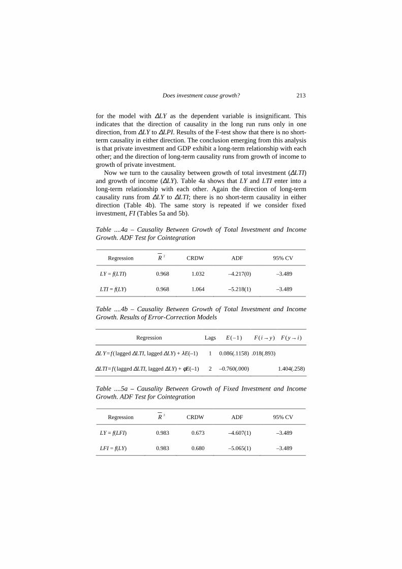
Does investment cause growth? 213
for the model with ∆LY as the dependent variable is insignificant. This indicates that the direction of causality in the long run runs only in one direction, from ∆LY to ∆LPI. Results of the F-test show that there is no short-term causality in either direction. The conclusion emerging from this analysis is that private investment and GDP exhibit a long-term relationship with each other; and the direction of long-term causality runs from growth of income to growth of private investment.
Now we turn to the causality between growth of total investment (∆LTI) and growth of income (∆LY). Table 4a shows that LY and LTI enter into a long-term relationship with each other. Again the direction of long-term causality runs from ∆LY to ∆LTI; there is no short-term causality in either direction (Table 4b). The same story is repeated if we consider fixed investment, FI (Tables 5a and 5b).
Table ....4a – Causality Between Growth of Total Investment and Income Growth. ADF Test for Cointegration
Regression R 2 CRDW ADF 95% CV
LY = f(LTI) 0.968 1.032 –4.217(0) –3.489
LTI = f(LY) 0.968 1.064 –5.218(1) –3.489
Table ....4b – Causality Between Growth of Total Investment and Income Growth. Results of Error-Correction Models
Regression Lags E(–1) F ( i →y) F (y→ i )
∆LY= f ( lagged ∆LTI, lagged ∆LY) + λE(–1) 1 0.086(.1158) .018(.893)
∆LTI= f ( lagged ∆LTI, lagged ∆LY) + φE(–1) 2 –0.760(.000) 1.404(.258)
Table ....5a – Causality Between Growth of Fixed Investment and Income Growth. ADF Test for Cointegration
Regression R 2 CRDW ADF 95% CV
LY = f(LFI) 0.983 0.673 –4.607(1) –3.489
LFI = f(LY) 0.983 0.680 –5.065(1) –3.489

214 Old and New Growth Theories: an Assessment
Table ....5b – Causality Between Growth of Fixed Investment and Income Growth. Results of Error-Correction Models
Regression Lags E(–1) F ( i →y) F (y→ i )
∆LY= f ( lagged ∆LFI, lagged ∆LY) + λE(–1) 1 .063(.432) .009(.923)
∆LFI = f ( lagged ∆LFI, lagged ∆LY) + φE(–1) 2 –0.443(.000) .028(.868)
Some authors (for example Sheehey, 1990) have argued that there is bound to be a problem of built-in correlation between GDP and any category (such as exports or investment) which is a substantial portion of GDP. To take account of this objection the above regressions were re-estimated after netting out the relevant investment variable from the GDP. Although the results are not reported here, this adjustment makes no difference to our results. Moreover, when the income variable is defined in terms of per capita income in place of GDP and the investment variable is defined as investment/GDP ratio, the results remain the same. It thus appears that the results are quite robust to the way we define the investment or income variable.
So the basic conclusion which emerges is that in India capital accumulation is the result rather than the cause of growth. This finding is in line with that obtained by other researchers such as Lipsey and Kravis (1987) and Blomstrom et al. (1996). The findings are also in consonance with the Young and Currie view that saving and investment are derivative rather than initiating factors of growth.
Our finding that the rate of capital accumulation exercises an insignificant influence over the rate of growth of the Indian economy is similar to that obtained by Chandra (2000). In a multivariate model involving the investment ratio and trade policy variables, he finds that the investment ratio has an insignificant impact on per capita income growth. This result contradicts the mainstream view that the investment rate is crucial to explaining growth, and this in turn requires an explanation.
This result, inter alia, may be the outcome of large unutilised capacity in Indian industry. Studies have shown that the protectionist policies of the past have had an adverse impact on capacity utilisation in India. For example, Paul (1974) and Goldar and Renganathan (1991) found a negative relationship between the effective rate of protection and the rate of capacity utilisation across industries. It appears that protection from foreign competition insulates domestic firms from any competitive pressures to reduce production costs by utilising capacity more fully. Moreover,

Does investment cause growth? 215
protectionist policies do not allow imported inputs and intermediates to be readily available, resulting in large unutilised capacity.
Other factors inhibiting fuller utilisation of capacity may include infrastructural bottlenecks (in the form of power shortage or transportation difficulties), shortage of domestic demand, incompatibility of the structure of capacities with the evolving structure of demand, and management deficiencies.
Large unutilised capacity may also result from archaic policies that prevent redeployment of resources from unproductive uses to more productive ones. For example, an industrial unit in India cannot be closed down unless permitted by the government and such permission is rarely forthcoming. Similarly, labour laws are heavily loaded in favour of labour, as a result of which it is almost impossible to retrench labour.9 Restructuring and redeployment of resources are an essential ingredient of competition; in India laws prohibit this. Competition is not only about easy entry but easy exit as well. In India an exit policy has yet to be evolved. As a result, large parts of her industry remain sick or unviable.
....5. CONCLUSIONS
Development literature has regarded accumulation of material capital as the key to growth; the emphasis has therefore been placed on increasing the rates of saving and investment in strategies followed by developing countries in the post-war period.
Indian planning has not deviated from this mainstream thinking. Accordingly, policies aimed at pushing up the rates of savings and investment were vigorously pursued. While India succeeded in pushing up the these rates from a low of 10% in the 1950s to around 22% by the end of 1970s, there was no commensurate increase in the growth rate.
Empirical investigation shows that no doubt there is a long-term positive relationship between investment and GDP in India, but the causality is from the latter to the former and not vice versa. The evidence suggests that in India capital accumulation does not cause growth in the long run; rather growth is the cause of capital accumulation, in line with the Young-Currie view.
In the case of government investment and GDP there is no long run relationship; and the short run relationship from government investment to growth actually appears to be negative.
The emerging conclusion is that investment may be important; but it is important in a derivative sense and not as a causative factor. Policy makers in India need to pay as much attention to the efficiency (or productivity) of investment as to investment itself. An environment needs to be created
216 Old and New Growth Theories: an Assessment
whereby those resources that are currently locked up in unproductive uses are allowed to be moved to more productive employments. The markets need to be enlarged and strengthened along with the institutional structures which are required for their efficient functioning. State intervention designed to replace and distort the markets is not likely to yield good results, as the Indian experience suggests.
It is not our intention to suggest that policy makers should de-emphasise investment;10 rather they should give equal importance to the demand-side view which regards higher saving and investment as a consequence of higher growth and not its primary cause. The policy-makers would therefore do well to give up their excessive obsession with a purely capital accumulation (supply side) approach and adopt a more balanced one which takes account of demand. Because increased demand in the overall sense means increased trade or reciprocal exchange, this requires that countries foster more competitive and internationally open markets.
In this way resources would flow more naturally to where they would yield the greatest social return with lowest prices and cost. The overall size of the market (reciprocal demand) is more rapidly extended if consumers’ purchasing power is increased through lower prices and more remunerative employment. These are the fruits of product–market competition, factor–market mobility, low inflation, and flexible prices including realistic exchange rates. As the market grows, so does the opportunity to extend the division of labour in ever more elaborate and productive ways, making innovation and ‘factor–productivity growth’ endogenous and cumulative. The role of the state would then be to create conditions for the rapid realization of increasing returns by strengthening and enhancing the market system and its institutions. In this circumstance lies the possibility of economic progress, as Allyn Young would have put it.
REFERENCES
Abramovitz, M. (1956), ‘Resources and output trends in the United States since 1870’, American Economic Review, Papers and Proceedings, 46, May, 5–23.
Aghion, P. and P. Howitt (1998), Endogenous Growth Theory, Cambridge, Massechussets: MIT Press.
Bahmani-Oskooee, M., H. Mohtadi, and G. Shabsigh (1991), ‘Exports, growth and causality in LDCs: a re-examination’, Journal of Development Economics, 36, October, 405–15.

Does investment cause growth? 217
Bahmani-Oskooee, M. and J. Alse (1993), ‘Export growth and economic growth: an application of cointegration and error-correction modelling’, The Journal of Developing Areas, 27, July, 535–42.
Bhagwati, J. (1993), India in Transition: Freeing the Economy, Oxford: Clarendon Press.
Blomström, M., R.E. Lipsey and M. Zejan (1996), ‘Is fixed investment the key to economic growth?’, Quarterly Journal of Economics, 111, February, 269–73.
Chakravarty, S. (1987), Development Planning: The Indian Experience, Oxford: Clarendon Press.
Chandra, Ramesh (2000), The Impact of Trade Policy on Growth in India, Unpublished Ph. D. Thesis, University of Strathclyde, Glasgow.
Currie, L. (1966) Accelerating Development: The Necessity and the Means, New York: McGraw-Hill Book Company.
Currie, L. (1974), ‘The leading sector model of growth in developing countries’, Journal of Economic Studies, 1.1, 1–16.
Currie, L. (1981), ‘Allyn Young and the development of growth theory’, Journal of Economic Studies, 8.1, 52–61.
Currie, L. (1997), ‘Implications of an endogenous theory of growth in Allyn Young’s macroeconomic concept of increasing returns’, History of Political Economy, 29(3), 413–43.
De Long, J.B. and L. Summers (1991), ‘Equipment investment and economic growth’, Quarterly Journal of Economics, CVI, 445–502.
De Long, J.B. and L. Summers (1992), ‘Equipment investment and economic growth: how strong is the nexus?’, Brookings Papers on Economic Activity, ....., 157–211.
Dickey, D.A. and W.F. Fuller (1979), ‘Distribution of the estimators for autoregressive time series with a unit root’, Journal of the American Statistical Association, 74, 427–31.
Domar, E.D. (1947) ‘Expansion of employment’, American Economic Review, March, ..........
Doraisami, A. (1996), ‘Export growth and economic growth: a re-examination of some time-series evidence of the Malaysian experience’, Journal of Developing Areas, 30, January, 223–30.
Engle, R.F. and C.W.J. Granger, (1987) ‘Cointegration and error correction: representation, estimation and testing’, Econometrica, 55, March, 251–76.

218 Old and New Growth Theories: an Assessment
Engle, R.F. and B.S. Yoo (1987), ‘Forecasting and testing in cointegrated systems’, Journal of Econometrics, 35, 143–59.
Goldar, B. and V.S. Renganathan (1991), ‘Capacity utilisation in Indian industries’, Indian Economic Journal, 39(2), 82–92.
Granger, C.W.J. (1969), ‘Investigating causal relations by econometric models and cross-spectral methods’, Econometrica, 37, 424–38.
Harrod, R.F. (1939), ‘An essay in dynamic theory’, Economic Journal, March, .......
Hsiao, M.W. (1987), ‘Tests of causality and exogeneity between export growth and economic growth’, Journal of Development Economics, 18, 143–59.
Jones, J.D. and D. Joulfaian (1991), ‘Federal government expenditures and revenues in the early years of the American Republic: evidence from 1972 and 1860’, Journal of Macroeconomics, 13(1), 133–55.
Kaldor, N. (1972), ‘The irrelevance of equilibrium economics’, Economic Journal, 82, 1237–55,
Krugman, P. (1990) Rethinking International Trade, Cambridge, Massachusetts: MIT Press.
Krugman, P. (1993), ‘Towards a counter-counterrevolution in development theory’, Annual Conference on Development Economics, Washington DC: The World Bank, 15–38.
Lewis, W.A. (1954), ‘Economic development with unlimited supplies of labour’, The Manchester School of Economics and Social Studies, XXII, 139–91.
Lipsey, R. and I. Kravis (1987), Saving and Economic Growth: Is the United States Really Falling Behind?, New York: The Conference Board.
Love, J. (1994), ‘Engines of growth: the exports and government sectors’, The World Economy, 17, 203–18.
MacKinnon, J.G. (1991), ‘Critical values for cointegration tests’, in R.F. Engle and C.W.J. Granger (eds), Long-Run Equilibrium Relationships, Oxford: Oxford University Press.
Mehrling, P.G. and R.J. Sandilands (1999), Money and Growth: Selected Papers of Allyn Abbott Young, London and New York: Routledge.
Murphy, K.M., A. Schleifer, and R. Vishny (1989a), ‘Income distribution, market size, and industrialization’, Quarterly Journal of Economics, 104(August), 537–64.
Murphy, K.M., A. Schleifer, and R. Vishny (1989b), ‘Industrialization and the big push’, Journal of Political Economy, 97(5), 1003–26.

Does investment cause growth? 219
Myrdal, G. (1957), Economic Theory and Underdeveloped Regions, London: Gerald Duckworth and Company Ltd..
Nurkse, R. (1953), Problems of Capital Formation in Underdeveloped Countries, Oxford: Basil Blackwell.
Nurkse, R. (1962), Patterns of Trade and Development (Wicksell Lectures, 1959), Oxford, Basil Blackwell.
Paul, S. (1974), ‘Industrial performance and government controls’, in J.C. Sandesara (ed.), The Indian Economy: Performance and Prospects, Bombay: Bombay University Press.
Perman, R. (1991), ‘Cointegration: an introduction to the literature’, Journal of Economic Studies, 18(3), 3–30.
Pesaran, M.H. and B. Pesaran (1997), Microfit 4.0, Oxford: Oxford University Press.
Phillips, P.C. and P. Perron (1988), ‘Testing for a unit root in a time series regression’, Biometrica, 75(2), 335–46.
Prebisch, R. (1950), The Economic Development of Latin America and its Principal Problems, New York: UN Economic Commission for Latin America.
Romer, P. (1987), ‘Growth based on increasing returns due to specialisation’, American Economic Review, 77(2), 56–62.
Romer, P. (1989), ‘Capital accumulation in the theory of long-run growth’, in R.J. Barro (ed.), Modern Business Cycle Theory, Cambridge, Massachusetts: Harvard University Press, pp. 52–127.
Rosenstein-Rodan, P.N. (1943), ‘Problems of industrialisation of Eastern and South-Eastern Europe’, Economic Journal, Vol. 53, 202–11.
Rosenstein-Rodan, P.N. (1961), ‘Notes on the theory of the ‘big push’’, in H.S. Ellis and H.C. Wallich (eds), Economic Development For Latin America, London: Macmillan.
Sandilands, R.J. (1990), The Life and Political Economy of Lauchlin Currie: New Dealer, Presidential Adviser, and Development Economist, Durham, NC and London: Duke University Press.
Sandilands, R.J. (2000), ‘Perspectives on Allyn Young in theories of endogenous growth’, Journal of the History of Economic Thought, 22(3), 309–28.
Shaw, G.K. (1992), ‘Policy implications of endogenous growth theory’ Economic Journal, 102(May), 611–21.
Sheehey, E.J. (1990), ‘Exports and growth: a flawed framework’, Journal of Development Studies, 27(1), 111–16.

220 Old and New Growth Theories: an Assessment
Sims, C.A. (1972), ‘Money, income and causality’, American Economic Review, 62(September), 540–52.
Singer, H.W. (1950), ‘The distribution of gains between investing and borrowing countries’, American Economic Review, 40(May), 473–85.
Solow, R.M. (1957), ‘Technical change and the aggregate production function’, Review of Economics and Statistics, 39(August), 311–20.
Toner, P. (1999), Main Currents in Cumulative Causation: The Dynamics of Growth and Development, London: Macmillan.
Young, A.A. (1928), ‘Increasing returns and economic progress’, Economic Journal, 38(December), 527–42.
NOTES
1. Nicholas Kaldor also developed a critique of equilibrium theory and instead emphasised the
role of demand and increasing returns (see, for example, Kaldor, 1972 and Toner, 1999). Sandilands (1990 and 2000) explains the parallels, but also some important differences, in the ‘Youngian’ interpretations of Kaldor and Currie. See also the editors’ preface in Mehrling and Sandilands (1999), a collection of Young’s writings that includes extracts from Kaldor’s notes on Young’s LSE lectures on growth theory.
2. Increased specialisation necessarily implies increased trade or exchange. Exchange implies a market demand. In the aggregate this is defined by GDP. Thus if capital follows GDP we have that capital follows upon demand in the aggregate, Say-Young conception. (A related issue is how far real Sayian demand is boosted when the government replaces the private market place. Note that Say’s Law was fully expressed as Say’s Law of Markets. While Keynes may have shown how Say’s Law may be interrupted by cyclical, short-term monetary disturbances, he assuredly did not bury it as a long-term ‘law’ for a world in which the demand for goods in general is still insatiable, and where government controls do not frustrate the operation of market forces.)
3. Compare Currie (1997) for an empirical investigation of the theory in the context of the United States.
4. A time series is stationary (in the sense of weak stationarity) if its mean, variance and covariances remain constant over time.
5. A correlogram is a graph of autocorrelation of a series at various lag levels. For a stationary time series, the correlogram tapers off quickly; for a non-stationary time series it dies off gradually.
6. Perman (1991) suggests that if the diagnostic statistics (such as normality, autocorrelation etc) from ADF regression are not in order a prima facie case exists for adopting non-parametric adjustments proposed by Phillips and Perron.
7. If a time series has to be differenced once before it becomes stationary, it is integrated to the order one; i.e., I(1). In general, if a time series has to be differenced d times before it becomes stationary, it is integrated to the order d or I(d).
8. Appendices containing data on all the level variables and their rates of growth, together with the graphs are available from the authors on request.

Does investment cause growth? 221
9. Pro-labour laws are, however, against the long-term interest of labour as they inhibit employers from offering formal employment to labour which cannot be retrenched. Moreover, the labour laws inhibit rapid growth of the industrial sector thereby inhibiting rapid expansion of employment opportunities.
10. Especially of the market-enhancing kind such as on transport and communications. Such public investments were viewed with approval even by Adam Smith.