Embed Size (px)
Citation preview
14.452 Economic Growth: Lecture 9, EndogenousTechnological Change
Daron Acemoglu
MIT
November 19, 2009.
Daron Acemoglu (MIT) Economic Growth Lecture 9 November 19, 2009. 1 / 60
Endogenous Technological Change Expanding Variety Models
Introduction
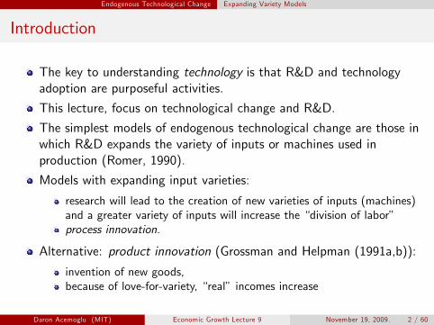
The key to understanding technology is that R&D and technology adoption are purposeful activities.
This lecture, focus on technological change and R&D.
The simplest models of endogenous technological change are those in which R&D expands the variety of inputs or machines used in production (Romer, 1990).
Models with expanding input varieties:
research will lead to the creation of new varieties of inputs (machines) and a greater variety of inputs will increase the “division of labor” process innovation.
Alternative: product innovation (Grossman and Helpman (1991a,b)):
invention of new goods, because of love-for-variety, “real” incomes increase
Daron Acemoglu (MIT) Economic Growth Lecture 9 November 19, 2009. 2 / 60
1
2
3
Endogenous Technological Change Expanding Variety Models
Key Insights
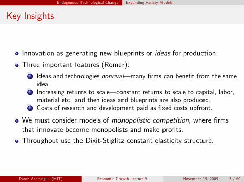
Innovation as generating new blueprints or ideas for production.
Three important features (Romer):
Ideas and technologies nonrival– many firms can benefit from the same idea. Increasing returns to scale– constant returns to scale to capital, labor, material etc. and then ideas and blueprints are also produced. Costs of research and development paid as fixed costs upfront.
We must consider models of monopolistic competition, where firms that innovate become monopolists and make profits.
Throughout use the Dixit-Stiglitz constant elasticity structure.
Daron Acemoglu (MIT) Economic Growth Lecture 9 November 19, 2009. 3 / 60
Baseline Expending Varieties Model The Lab Equipment Model
The Lab Equipment Model with Input Varieties
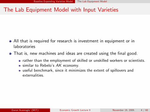
All that is required for research is investment in equipment or in laboratories
That is, new machines and ideas are created using the final good.
rather than the employment of skilled or unskilled workers or scientists. similar to Rebelo’s AK economy. useful benchmark, since it minimizes the extent of spillovers and externalities.
Daron Acemoglu (MIT) Economic Growth Lecture 9 November 19, 2009. 4 / 60
Baseline Expending Varieties Model The Lab Equipment Model
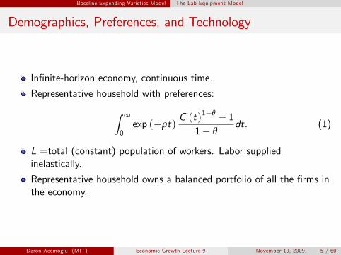
Demographics, Preferences, and Technology
Infinite-horizon economy, continuous time.
Representative household with preferences:
� ∞ 1−θ
exp (−ρt) C (t
1 ) − θ − 1
dt. (1) 0
L =total (constant) population of workers. Labor supplied inelastically.
Representative household owns a balanced portfolio of all the firms in the economy.
Daron Acemoglu (MIT) Economic Growth Lecture 9 November 19, 2009. 5 / 60
Baseline Expending Varieties Model The Lab Equipment Model
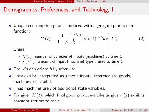
Demographics, Preferences, and Technology I
Unique consumption good, produced with aggregate production function: �� N (t)
�
Y (t) = 1
x(ν, t)1−βdν Lβ , (2)1 − β 0
where
N (t)=number of varieties of inputs (machines) at time t, x (ν, t)=amount of input (machine) type ν used at time t.
The x’s depreciate fully after use.
They can be interpreted as generic inputs, intermediate goods, machines, or capital.
Thus machines are not additional state variables.
For given N (t), which final good producers take as given, (2) exhibits constant returns to scale.
Daron Acemoglu (MIT) Economic Growth Lecture 9 November 19, 2009. 6 / 60
Baseline Expending Varieties Model The Lab Equipment Model
Demographics, Preferences, and Technology II
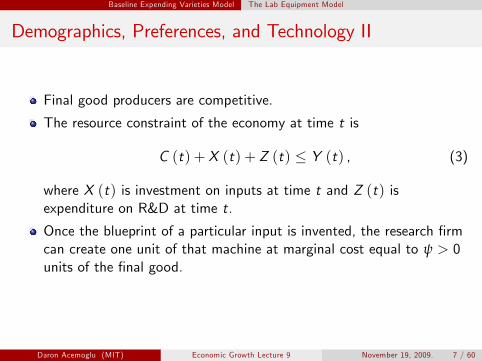
Final good producers are competitive.
The resource constraint of the economy at time t is
C (t) + X (t) + Z (t) ≤ Y (t) , (3)
where X (t) is investment on inputs at time t and Z (t) is expenditure on R&D at time t.
Once the blueprint of a particular input is invented, the research firm can create one unit of that machine at marginal cost equal to ψ > 0 units of the final good.
Daron Acemoglu (MIT) Economic Growth Lecture 9 November 19, 2009. 7 / 60
Baseline Expending Varieties Model The Lab Equipment Model
Innovation Possibilities Frontier and Patents I
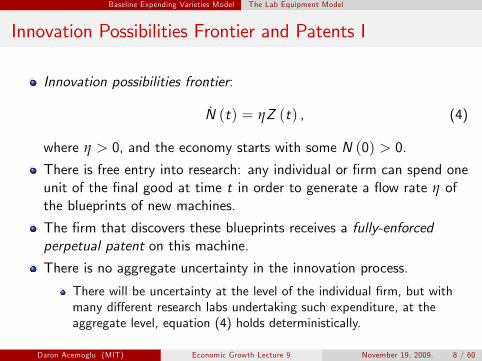
Innovation possibilities frontier:
N (t) = ηZ (t) , (4)
where η > 0, and the economy starts with some N (0) > 0.
There is free entry into research: any individual or firm can spend one unit of the final good at time t in order to generate a fiow rate η of the blueprints of new machines.
The firm that discovers these blueprints receives a fully-enforced perpetual patent on this machine.
There is no aggregate uncertainty in the innovation process.
There will be uncertainty at the level of the individual firm, but with many different research labs undertaking such expenditure, at the aggregate level, equation (4) holds deterministically.
Daron Acemoglu (MIT) Economic Growth Lecture 9 November 19, 2009. 8 / 60
Baseline Expending Varieties Model The Lab Equipment Model
Innovation Possibilities Frontier and Patents II
A firm that invents a new machine variety v is the sole supplier of that type of machine, and sets a profit-maximizing price of px (ν, t) at time t to maximize profits.
Since machines depreciate after use, px (ν, t) can also be interpreted as a “rental price” or the user cost of this machine.
Daron Acemoglu (MIT) Economic Growth Lecture 9 November 19, 2009. 9 / 60
Baseline Expending Varieties Model The Lab Equipment Model
The Final Good Sector
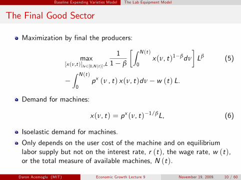
Maximization by final the producers:
max 1
�� N (t) x(ν, t)1−βdν
�
Lβ (5) [x (ν,t)]lv ∈[0,N (t)],L 1 − β 0 � N (t) −
0 px (ν , t) x(ν, t)dν − w (t) L.
Demand for machines:
x(ν, t) = px (ν, t)−1/βL, (6)
Isoelastic demand for machines.
Only depends on the user cost of the machine and on equilibrium labor supply but not on the interest rate, r (t), the wage rate, w (t), or the total measure of available machines, N (t).
Daron Acemoglu (MIT) Economic Growth Lecture 9 November 19, 2009. 10 / 60
Baseline Expending Varieties Model The Lab Equipment Model
Profit Maximization by Technology Monopolists I
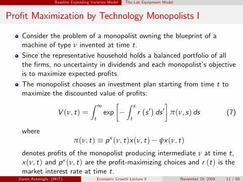
Consider the problem of a monopolist owning the blueprint of a machine of type ν invented at time t.
Since the representative household holds a balanced portfolio of all the firms, no uncertainty in dividends and each monopolist’s objective is to maximize expected profits.
The monopolist chooses an investment plan starting from time t to maximize the discounted value of profits: � ∞
� � s � � �
V (ν, t) = exp r s � ds � π(ν, s) ds (7) t
− t
where π(ν, t) ≡ px (ν, t)x(ν, t) − ψx(ν, t)
denotes profits of the monopolist producing intermediate ν at time t, x(ν, t) and px (ν, t) are the profit-maximizing choices and r (t) is the market interest rate at time t.
Daron Acemoglu (MIT) Economic Growth Lecture 9 November 19, 2009. 11 / 60
1
2
Baseline Expending Varieties Model The Lab Equipment Model
Profit Maximization by Technology Monopolists II
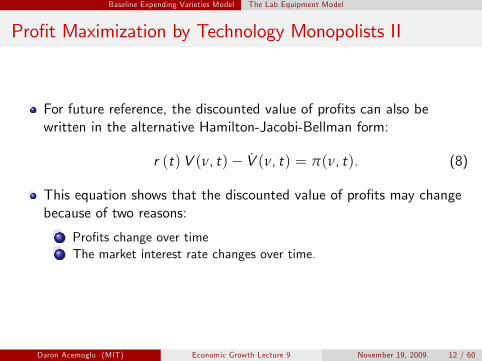
For future reference, the discounted value of profits can also be written in the alternative Hamilton-Jacobi-Bellman form:
r (t) V (ν, t) − V (ν, t) = π(ν, t). (8)
This equation shows that the discounted value of profits may change because of two reasons:
Profits change over time The market interest rate changes over time.
Daron Acemoglu (MIT) Economic Growth Lecture 9 November 19, 2009. 12 / 60
Baseline Expending Varieties Model The Lab Equipment Model
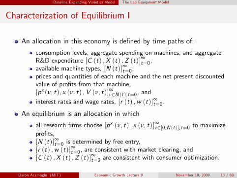
Characterization of Equilibrium I
An allocation in this economy is defined by time paths of:
consumption levels, aggregate spending on machines, and aggregate R&D expenditure [C (t) , X (t) , Z (t)]t
∞ =0,
available machine types, [N (t)]t∞ =0,
prices and quantities of each machine and the net present discounted value of profits from that machine, [px (ν, t), x (ν, t) , V (ν, t)]∞
ν∈N (t),t=0, and
interest rates and wage rates, [r (t) , w (t)] ∞ t=0.
An equilibrium is an allocation in which
all research firms choose [px (ν, t) , x (ν, t)]∞ ν∈[0,N (t)],t=0 to maximize
profits, [N (t)] t
∞ =0 is determined by free entry,
[r (t) , w (t)] t ∞ =0, are consistent with market clearing, and
[C (t) , X (t) , Z (t)]t ∞ =0 are consistent with consumer optimization.
Daron Acemoglu (MIT) Economic Growth Lecture 9 November 19, 2009. 13 / 60
Baseline Expending Varieties Model The Lab Equipment Model
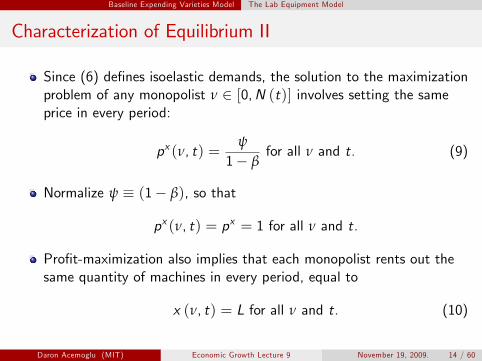
Characterization of Equilibrium II
Since (6) defines isoelastic demands, the solution to the maximization problem of any monopolist ν ∈ [0, N (t)] involves setting the same price in every period:
ψ px (ν, t) = for all ν and t. (9)
1 − β
Normalize ψ ≡ (1 − β), so that
px (ν, t) = px = 1 for all ν and t.
Profit-maximization also implies that each monopolist rents out the same quantity of machines in every period, equal to
x (ν, t) = L for all ν and t. (10)
Daron Acemoglu (MIT) Economic Growth Lecture 9 November 19, 2009. 14 / 60
Baseline Expending Varieties Model The Lab Equipment Model
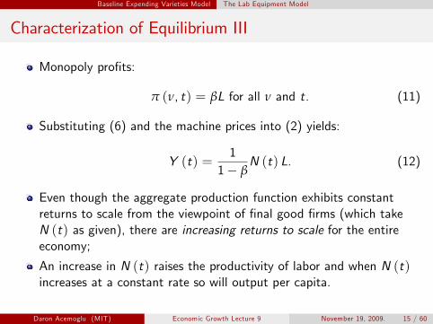
Characterization of Equilibrium III
Monopoly profits:
π (ν, t) = βL for all ν and t. (11)
Substituting (6) and the machine prices into (2) yields:
1Y (t) = N (t) L. (12)
1 − β
Even though the aggregate production function exhibits constant returns to scale from the viewpoint of final good firms (which take N (t) as given), there are increasing returns to scale for the entire economy;
An increase in N (t) raises the productivity of labor and when N (t) increases at a constant rate so will output per capita.
Daron Acemoglu (MIT) Economic Growth Lecture 9 November 19, 2009. 15 / 60
Baseline Expending Varieties Model The Lab Equipment Model
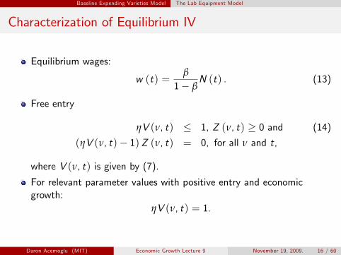
Characterization of Equilibrium IV
Equilibrium wages: β
w (t) = N (t) . (13)1 − β
Free entry
ηV (ν, t) ≤ 1, Z (ν, t) ≥ 0 and (14)
(ηV (ν, t) − 1) Z (ν, t) = 0, for all ν and t,
where V (ν, t) is given by (7).
For relevant parameter values with positive entry and economic growth:
ηV (ν, t) = 1.
Daron Acemoglu (MIT) Economic Growth Lecture 9 November 19, 2009. 16 / 60
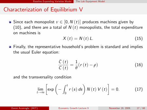
Baseline Expending Varieties Model The Lab Equipment Model
Characterization of Equilibrium V
Since each monopolist ν ∈ [0, N (t)] produces machines given by (10), and there are a total of N (t) monopolists, the total expenditure on machines is
X (t) = N (t) L. (15)
Finally, the representative household’s problem is standard and implies the usual Euler equation:
C (t) 1 C (t)
= θ (r (t) − ρ) (16)
and the transversality condition � � � t � �
tlim
∞ exp −
0 r (s) ds N (t) V (t) = 0. (17)
→
Daron Acemoglu (MIT) Economic Growth Lecture 9 November 19, 2009. 17 / 60
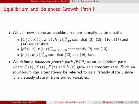
Baseline Expending Varieties Model The Lab Equipment Model
Equilibrium and Balanced Growth Path I
We can now define an equilibrium more formally as time paths ∞[C (t) , X (t) , Z (t) , N (t)] t=0, such that (3), (15), (16), (17) and
(14) are satisfied; ∞[px (ν, t) , x (ν, t)]ν∈N (t),t=0 that satisfy (9) and (10),
[r (t) , w (t)] t ∞ =0 such that (13) and (16) hold.
We define a balanced growth path (BGP) as an equilibrium path where C (t) , X (t) , Z (t) and N (t) grow at a constant rate. Such an equilibrium can alternatively be referred to as a “steady state”, since it is a steady state in transformed variables.
Daron Acemoglu (MIT) Economic Growth Lecture 9 November 19, 2009. 18 / 60
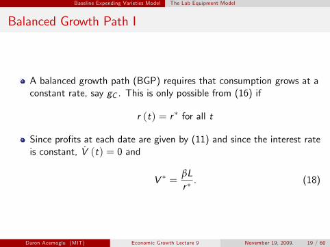
Baseline Expending Varieties Model The Lab Equipment Model
Balanced Growth Path I
A balanced growth path (BGP) requires that consumption grows at a constant rate, say gC . This is only possible from (16) if
r (t) = r ∗ for all t
Since profits at each date are given by (11) and since the interest rate is constant, V (t) = 0 and
βLV ∗ = . (18)
r ∗
Daron Acemoglu (MIT) Economic Growth Lecture 9 November 19, 2009. 19 / 60
Baseline Expending Varieties Model The Lab Equipment Model
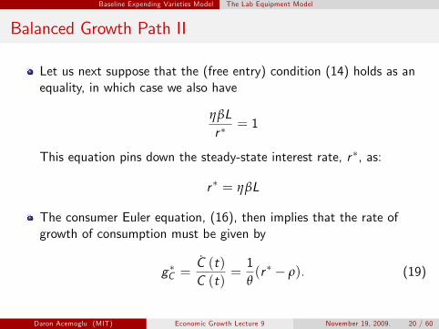
Balanced Growth Path II
Let us next suppose that the (free entry) condition (14) holds as an equality, in which case we also have
ηβL = 1
r ∗
This equation pins down the steady-state interest rate, r ∗, as:
r ∗ = ηβL
The consumer Euler equation, (16), then implies that the rate of growth of consumption must be given by
g ∗ = CC
˙ ((
tt)
) = 1 θ (r ∗ − ρ). (19)C
Daron Acemoglu (MIT) Economic Growth Lecture 9 November 19, 2009. 20 / 60
Baseline Expending Varieties Model The Lab Equipment Model
Balanced Growth Path III
Note the current-value Hamiltonian for the consumer’s maximization problem is concave, thus this condition, together with the transversality condition, characterizes the optimal consumption plans of the consumer.
In BGP, consumption grows at the same rate as total output
g ∗ = gC∗ .
Therefore, given r ∗, the long-run growth rate of the economy is:
1 g ∗ = (ηβL − ρ) (20)
θ
Suppose that ηβL > ρ and (1 − θ) ηβL < ρ, (21)
which will ensure that g ∗ > 0 and that the transversality condition is satisfied.
Daron Acemoglu (MIT) Economic Growth Lecture 9 November 19, 2009. 21 / 60
Baseline Expending Varieties Model The Lab Equipment Model
Balanced Growth Path IV
Proposition Suppose that condition (21) holds. Then, in the above-described lab equipment expanding input variety model, there exists a unique balanced growth path in which technology, output and consumption all grow at the same rate, g ∗, given by (20)..
An important feature of this class models is the presence of the scale effect: the larger is L, the greater is the growth rate.
Daron Acemoglu (MIT) Economic Growth Lecture 9 November 19, 2009. 22 / 60
Baseline Expending Varieties Model The Lab Equipment Model
Transitional Dynamics I
There are no transitional dynamics in this model.
Substituting for profits in the value function for each monopolist, this gives
r (t) V (ν, t) − V (ν, t) = βL.
The key observation is that positive growth at any point implies that ηV (ν, t) = 1 for all t. In other words, if ηV (ν, t �) = 1 for some t �, then ηV (ν, t) = 1 for all t.
Now differentiating ηV (ν, t) = 1 with respect to time yields V (ν, t) = 0, which is only consistent with r (t) = r ∗ for all t, thus
r (t) = ηβL for all t.
Daron Acemoglu (MIT) Economic Growth Lecture 9 November 19, 2009. 23 / 60
Baseline Expending Varieties Model The Lab Equipment Model
Transitional Dynamics II
Proposition Suppose that condition (21) holds. In the above-described lab equipment expanding input-variety model, with initial technology stock N (0) > 0, there is a unique equilibrium path in which technology, output and consumption always grow at the rate g ∗ as in (20).
While the microfoundations here are very different from the neoclassical AK economy, the mathematical structure is very similar to the AK model (as most clearly illustrated by the derived equation for output, (12)).
Consequently, as in the AK model, the economy always grows at a constant rate.
But the economics is very different.
Daron Acemoglu (MIT) Economic Growth Lecture 9 November 19, 2009. 24 / 60
1
2
Baseline Expending Varieties Model Pareto Optimal Allocations
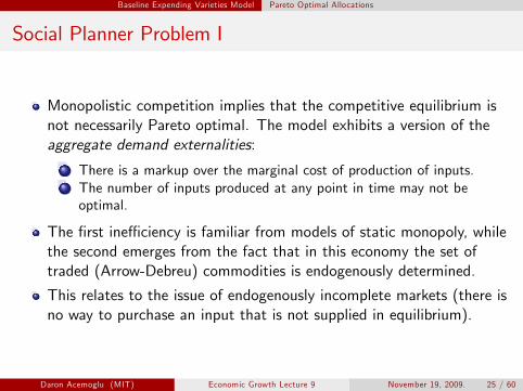
Social Planner Problem I
Monopolistic competition implies that the competitive equilibrium is not necessarily Pareto optimal. The model exhibits a version of the aggregate demand externalities:
There is a markup over the marginal cost of production of inputs. The number of inputs produced at any point in time may not be optimal.
The first ineffi ciency is familiar from models of static monopoly, while the second emerges from the fact that in this economy the set of traded (Arrow-Debreu) commodities is endogenously determined.
This relates to the issue of endogenously incomplete markets (there is no way to purchase an input that is not supplied in equilibrium).
Daron Acemoglu (MIT) Economic Growth Lecture 9 November 19, 2009. 25 / 60
Baseline Expending Varieties Model Pareto Optimal Allocations
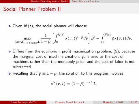
Social Planner Problem II
Given N (t), the social planner will choose
max 1
�� N (t ) x(ν, t)1−βdν
�
Lβ � N (t)
ψx(ν, t)dν, [x (ν,t)] v ∈[0,N (t)],L 1 − β 0
− 0
Differs from the equilibrium profit maximization problem, (5), because the marginal cost of machine creation, ψ, is used as the cost of machines rather than the monopoly price, and the cost of labor is not subtracted.
Recalling that ψ ≡ 1 − β, the solution to this program involves
xS (ν, t) = (1 − β)−1/β L,
Daron Acemoglu (MIT) Economic Growth Lecture 9 November 19, 2009. 26 / 60
Baseline Expending Varieties Model Pareto Optimal Allocations
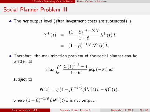
Social Planner Problem III
The net output level (after investment costs are subtracted) is
Y S (t) = (1 − β)−(1−β)/β
NS (t) L1 − β
= (1 − β)−1/β NS (t) L,
Therefore, the maximization problem of the social planner can be written as
max �
0
∞ C (t1 )1
−
−θ
θ − 1
exp (−ρt) dt
subject to
N (t) = η (1 − β)−1/β βN (t) L − ηC (t) .
where (1 − β)−1/β βNS (t) L is net output.
Daron Acemoglu (MIT) Economic Growth Lecture 9 November 19, 2009. 27 / 60
� �
Baseline Expending Varieties Model Pareto Optimal Allocations
Social Planner Problem IV
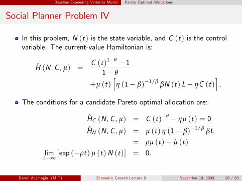
In this problem, N (t) is the state variable, and C (t) is the control variable. The current-value Hamiltonian is:
H (N, C , µ) = C (t)1−θ − 1
1 − θ
+µ (t) η (1 − β)−1/β βN (t) L − ηC (t) .
The conditions for a candidate Pareto optimal allocation are:
H C (N, C , µ) = C (t)−θ − ηµ (t) = 0
H N (N, C , µ) = µ (t) η (1 − β)−1/β βL
= ρµ (t) − µ (t) lim [exp (−ρt) µ (t) N (t)] = 0. t ∞→
Daron Acemoglu (MIT) Economic Growth Lecture 9 November 19, 2009. 28 / 60
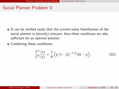
Baseline Expending Varieties Model Pareto Optimal Allocations
Social Planner Problem V
It can be verified easily that the current-value Hamiltonian of the social planner is (strictly) concave, thus these conditions are also suffi cient for an optimal solution.
Combining these conditions:
C S (t) 1 � −1/β
�
CS (t)=
θη (1 − β) βL − ρ . (22)
Daron Acemoglu (MIT) Economic Growth Lecture 9 November 19, 2009. 29 / 60
Baseline Expending Varieties Model Pareto Optimal Allocations
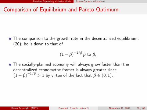
Comparison of Equilibrium and Pareto Optimum
The comparison to the growth rate in the decentralized equilibrium, (20), boils down to that of
(1 − β)−1/β β to β,
The socially-planned economy will always grow faster than the decentralized economythe former is always greater since (1 − β)−1/β > 1 by virtue of the fact that β ∈ (0, 1).
Daron Acemoglu (MIT) Economic Growth Lecture 9 November 19, 2009. 30 / 60
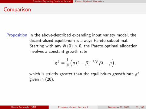
Baseline Expending Varieties Model Pareto Optimal Allocations
Comparison
Proposition In the above-described expanding input variety model, the decentralized equilibrium is always Pareto suboptimal. Starting with any N (0) > 0, the Pareto optimal allocation involves a constant growth rate
gS = 1 �
η (1 − β)−1/β βL − ρ � ,
θ
which is strictly greater than the equilibrium growth rate g ∗
given in (20).
Daron Acemoglu (MIT) Economic Growth Lecture 9 November 19, 2009. 31 / 60

Baseline Expending Varieties Model Pareto Optimal Allocations
Comparison
Why is the equilibrium growing more slowly than the optimum allocation?
Because the social planner values innovation more
The social planner is able to use the machines more intensively after innovation, pecuniary externality resulting from the monopoly markups.
Other models of endogenous technological progress we will study in this lecture incorporate technological spillovers and thus generate ineffi ciencies both because of the pecuniary externality isolated here and because of the standard technological spillovers.
Daron Acemoglu (MIT) Economic Growth Lecture 9 November 19, 2009. 32 / 60

1
2
Baseline Expending Varieties Model Pareto Optimal Allocations
Policies
What kind of policies can increase equilibrium growth rate?
Subsidies to Research: the government can increase the growth rate of the economy, and this can be a Pareto improvement if taxation is not distortionary and there can be appropriate redistribution of resources so that all parties benefit.
Subsidies to Capital Inputs: ineffi ciencies also arise from the fact that the decentralized economy is not using as many units of the machines/capital inputs (because of the monopoly markup); so subsidies to capital inputs given to final good producers would also increase the growth rate.
But note, the same policies can also be used to distort allocations.
When we look at a the cross-section of countries, taxes on research and capital inputs more common than subsidies.
Daron Acemoglu (MIT) Economic Growth Lecture 9 November 19, 2009. 33 / 60
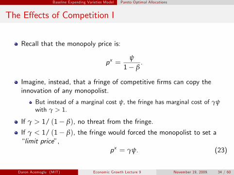
Baseline Expending Varieties Model Pareto Optimal Allocations
The Effects of Competition I
Recall that the monopoly price is:
ψxp = .1 − β
Imagine, instead, that a fringe of competitive firms can copy the innovation of any monopolist.
But instead of a marginal cost ψ, the fringe has marginal cost of γψ with γ > 1.
If γ > 1/ (1 − β), no threat from the fringe.
If γ < 1/ (1 − β), the fringe would forced the monopolist to set a “limit price”,
px = γψ. (23)
Daron Acemoglu (MIT) Economic Growth Lecture 9 November 19, 2009. 34 / 60
Baseline Expending Varieties Model Pareto Optimal Allocations
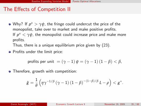
The Effects of Competition II
Why? If px > γψ, the fringe could undercut the price of the monopolist, take over to market and make positive profits. If px < γψ, the monopolist could increase price and make more profits. Thus, there is a unique equilibrium price given by (23).
Profits under the limit price:
profits per unit = (γ − 1) ψ = (γ − 1) (1 − β) < β,
Therefore, growth with competition:
g = 1 �
ηγ−1/β (γ − 1) (1 − β)−(1−β)/β L − ρ � < g ∗ .
θ
Daron Acemoglu (MIT) Economic Growth Lecture 9 November 19, 2009. 35 / 60
Baseline Expending Varieties Model Pareto Optimal Allocations
Growth with Knowledge Spillovers I
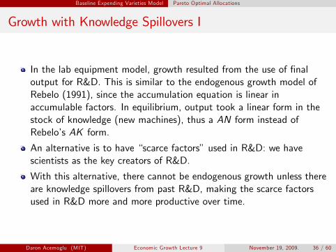
In the lab equipment model, growth resulted from the use of final output for R&D. This is similar to the endogenous growth model of Rebelo (1991), since the accumulation equation is linear in accumulable factors. In equilibrium, output took a linear form in the stock of knowledge (new machines), thus a AN form instead of Rebelo’s AK form.
An alternative is to have “scarce factors” used in R&D: we have scientists as the key creators of R&D.
With this alternative, there cannot be endogenous growth unless there are knowledge spillovers from past R&D, making the scarce factors used in R&D more and more productive over time.
Daron Acemoglu (MIT) Economic Growth Lecture 9 November 19, 2009. 36 / 60
Baseline Expending Varieties Model Pareto Optimal Allocations
Innovation Possibilities Frontier I
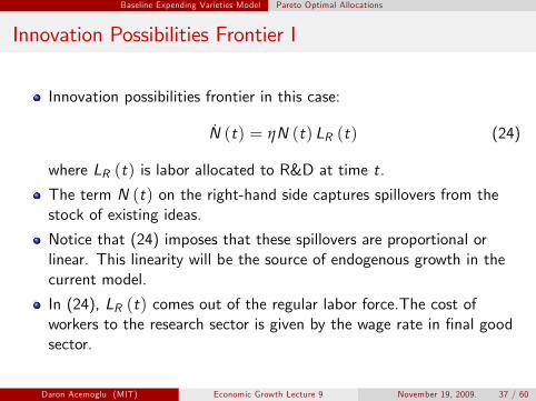
Innovation possibilities frontier in this case:
N (t) = ηN (t) LR (t) (24)
where LR (t) is labor allocated to R&D at time t.
The term N (t) on the right-hand side captures spillovers from the stock of existing ideas.
Notice that (24) imposes that these spillovers are proportional or linear. This linearity will be the source of endogenous growth in the current model.
In (24), LR (t) comes out of the regular labor force.The cost of workers to the research sector is given by the wage rate in final good sector.
Daron Acemoglu (MIT) Economic Growth Lecture 9 November 19, 2009. 37 / 60
Baseline Expending Varieties Model Pareto Optimal Allocations
Characterization of Equilibrium I
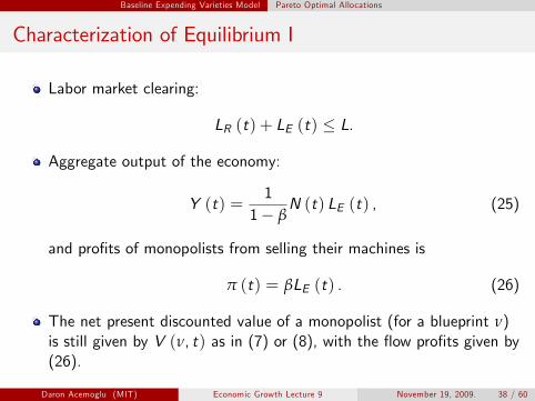
Labor market clearing:
LR (t) + LE (t) ≤ L.
Aggregate output of the economy:
1Y (t) = N (t) LE (t) , (25)
1 − β
and profits of monopolists from selling their machines is
π (t) = βLE (t) . (26)
The net present discounted value of a monopolist (for a blueprint ν) is still given by V (ν, t) as in (7) or (8), with the fiow profits given by (26).
Daron Acemoglu (MIT) Economic Growth Lecture 9 November 19, 2009. 38 / 60
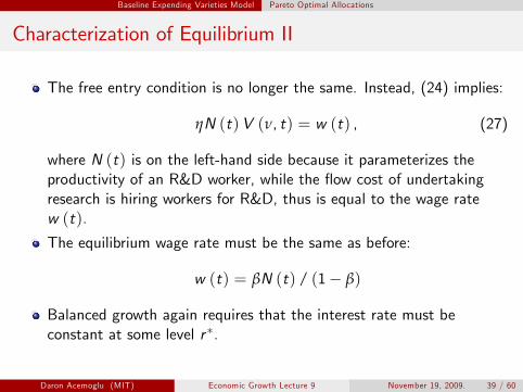
Baseline Expending Varieties Model Pareto Optimal Allocations
Characterization of Equilibrium II
The free entry condition is no longer the same. Instead, (24) implies:
ηN (t) V (ν, t) = w (t) , (27)
where N (t) is on the left-hand side because it parameterizes theproductivity of an R&D worker, while the fiow cost of undertakingresearch is hiring workers for R&D, thus is equal to the wage ratew (t).
The equilibrium wage rate must be the same as before:
w (t) = βN (t) / (1 − β)
Balanced growth again requires that the interest rate must beconstant at some level r ∗.
Daron Acemoglu (MIT) Economic Growth Lecture 9 November 19, 2009. 39 / 60
Baseline Expending Varieties Model Pareto Optimal Allocations
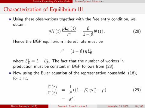
Characterization of Equilibrium III
Using these observations together with the free entry condition, we obtain:
βLE (t) β ηN (t) = N (t) . (28)
r ∗ 1 − β
Hence the BGP equilibrium interest rate must be
r ∗ = (1 − β) ηLE ∗ ,
where L∗ = L − LR ∗ . The fact that the number of workers in E
production must be constant in BGP follows from (28).
Now using the Euler equation of the representative household, (16), for all t:
C (t) C (t)
= 1 ((1 − β) ηLE
∗ − ρ)θ
(29)
∗≡ g .
Daron Acemoglu (MIT) Economic Growth Lecture 9 November 19, 2009. 40 / 60
Baseline Expending Varieties Model Pareto Optimal Allocations
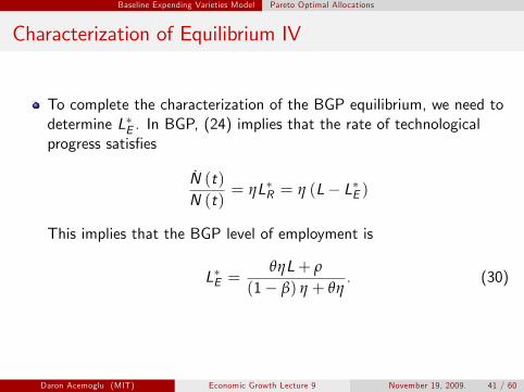
Characterization of Equilibrium IV
To complete the characterization of the BGP equilibrium, we need to determine LE
∗ . In BGP, (24) implies that the rate of technological progress satisfies
N (t)N (t)
= ηLR ∗ = η (L − LE
∗ )
This implies that the BGP level of employment is
θηL + ρLE ∗ = . (30)
(1 − β) η + θη
Daron Acemoglu (MIT) Economic Growth Lecture 9 November 19, 2009. 41 / 60
Baseline Expending Varieties Model Pareto Optimal Allocations
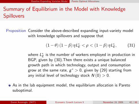
Summary of Equilibrium in the Model with Knowledge Spillovers
Proposition Consider the above-described expanding input-variety model with knowledge spillovers and suppose that
(1 − θ) (1 − β) ηL∗ E < ρ < (1 − β) ηLE ∗ , (31)
where LE ∗ is the number of workers employed in production in
BGP, given by (30).Then there exists a unique balanced growth path in which technology, output and consumption grow at the same rate, g ∗ > 0, given by (29) starting from any initial level of technology stock N (0) > 0.
As in the lab equipment model, the equilibrium allocation is Pareto suboptimal.
Daron Acemoglu (MIT) Economic Growth Lecture 9 November 19, 2009. 42 / 60
1
2
3
Scale Effects Growth without Scale Effects
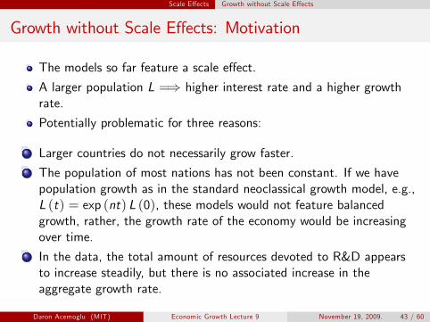
Growth without Scale Effects: Motivation
The models so far feature a scale effect.
A larger population L = higher interest rate and a higher growth⇒rate.
Potentially problematic for three reasons:
Larger countries do not necessarily grow faster.
The population of most nations has not been constant. If we have population growth as in the standard neoclassical growth model, e.g., L (t) = exp (nt) L (0), these models would not feature balanced growth, rather, the growth rate of the economy would be increasing over time.
In the data, the total amount of resources devoted to R&D appears to increase steadily, but there is no associated increase in the aggregate growth rate.
Daron Acemoglu (MIT) Economic Growth Lecture 9 November 19, 2009. 43 / 60
1
2
Scale Effects Growth without Scale Effects
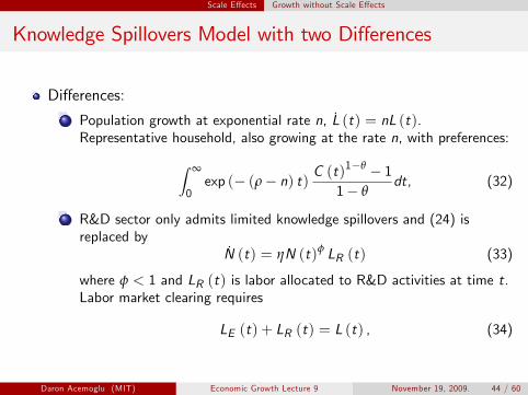
Knowledge Spillovers Model with two Differences
Differences:
Population growth at exponential rate n, L (t) = nL (t). Representative household, also growing at the rate n, with preferences:
� ∞ 1−θC (t) − 1 exp (− (ρ − n) t) dt,
0 1 − θ (32)
R&D sector only admits limited knowledge spillovers and (24) is replaced by
N (t) = ηN (t)φ LR (t) (33)
where φ < 1 and LR (t) is labor allocated to R&D activities at time t. Labor market clearing requires
LE (t) + LR (t) = L (t) , (34)
Daron Acemoglu (MIT) Economic Growth Lecture 9 November 19, 2009. 44 / 60
Scale Effects Growth without Scale Effects
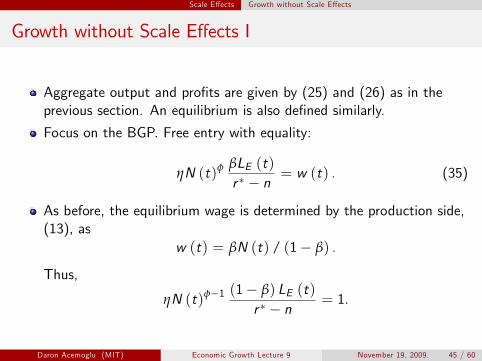
Growth without Scale Effects I
Aggregate output and profits are given by (25) and (26) as in the previous section. An equilibrium is also defined similarly.
Focus on the BGP. Free entry with equality:
ηN (t)φ βLE (t) = w (t) . (35)r ∗ − n
As before, the equilibrium wage is determined by the production side, (13), as
w (t) = βN (t) / (1 − β) .
Thus,
ηN (t)φ−1 (1 − β) LE (t) = 1. r ∗ − n
Daron Acemoglu (MIT) Economic Growth Lecture 9 November 19, 2009. 45 / 60
Scale Effects Growth without Scale Effects
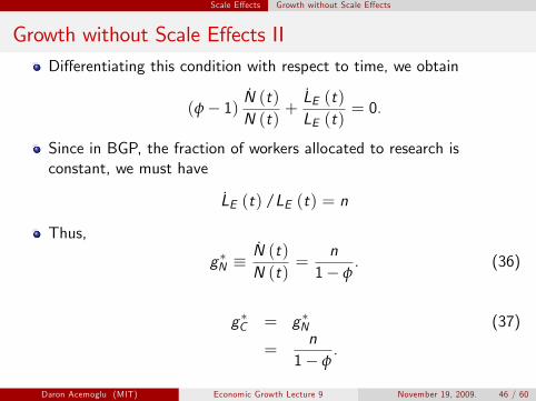
Growth without Scale Effects II Differentiating this condition with respect to time, we obtain
N (t) L E (t)(φ − 1)
N (t)+ LE (t)
= 0.
Since in BGP, the fraction of workers allocated to research is constant, we must have
L E (t) /LE (t) = n
Thus,
gN ∗ ≡
NN
˙ ((
tt)
) = 1 − n
φ . (36)
gC∗ = gN
∗ (37) n
= .1 − φ
Daron Acemoglu (MIT) Economic Growth Lecture 9 November 19, 2009. 46 / 60
Scale Effects Growth without Scale Effects
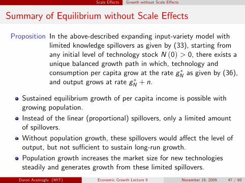
Summary of Equilibrium without Scale Effects
Proposition In the above-described expanding input-variety model with limited knowledge spillovers as given by (33), starting from any initial level of technology stock N (0) > 0, there exists a unique balanced growth path in which, technology and consumption per capita grow at the rate gN
∗ as given by (36), and output grows at rate gN
∗ + n.
Sustained equilibrium growth of per capita income is possible with growing population.
Instead of the linear (proportional) spillovers, only a limited amount of spillovers.
Without population growth, these spillovers would affect the level of output, but not suffi cient to sustain long-run growth.
Population growth increases the market size for new technologies steadily and generates growth from these limited spillovers.
Daron Acemoglu (MIT) Economic Growth Lecture 9 November 19, 2009. 47 / 60
1
2
Scale Effects Growth without Scale Effects
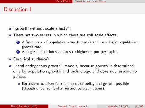
Discussion I
“Growth without scale effects”?
There are two senses in which there are still scale effects:
A faster rate of population growth translates into a higher equilibrium growth rate. A larger population size leads to higher output per capita.
Empirical evidence?
“Semi-endogenous growth” models, because growth is determined only by population growth and technology, and does not respond to policies.
Extensions to allow for the impact of policy and growth possible (though under somewhat restrictive assumptions).
Daron Acemoglu (MIT) Economic Growth Lecture 9 November 19, 2009. 48 / 60
Expanding Product Varieties Growth with Expanding Product Varieties
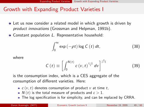
Growth with Expanding Product Varieties I
Let us now consider a related model in which growth is driven by product innovations (Grossman and Helpman, 1991b).
Constant population L. Representative household: � ∞ exp (−ρt) log C (t) dt, (38)
0
where �� N (t) ε−1 �
ε−ε 1
εC (t) ≡ c (ν, t) dν (39) 0
is the consumption index, which is a CES aggregate of theconsumption of different varieties. Here:
c (ν, t) denotes consumption of product ν at time t, N (t) is the total measure of products and ε > 1. The log specification is for simplicity, and can be replaced by CRRA.
Daron Acemoglu (MIT) Economic Growth Lecture 9 November 19, 2009. 49 / 60
Expanding Product Varieties Growth with Expanding Product Varieties
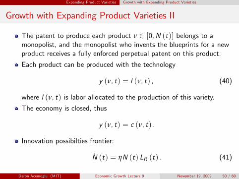
Growth with Expanding Product Varieties II
The patent to produce each product ν ∈ [0, N (t)] belongs to a monopolist, and the monopolist who invents the blueprints for a new product receives a fully enforced perpetual patent on this product.
Each product can be produced with the technology
y (ν, t) = l (ν, t) , (40)
where l (ν, t) is labor allocated to the production of this variety.
The economy is closed, thus
y (ν, t) = c (ν, t) .
Innovation possibilties frontier:
N (t) = ηN (t) LR (t) . (41)
Daron Acemoglu (MIT) Economic Growth Lecture 9 November 19, 2009. 50 / 60
Expanding Product Varieties Growth with Expanding Product Varieties
Growth with Expanding Product Varieties III
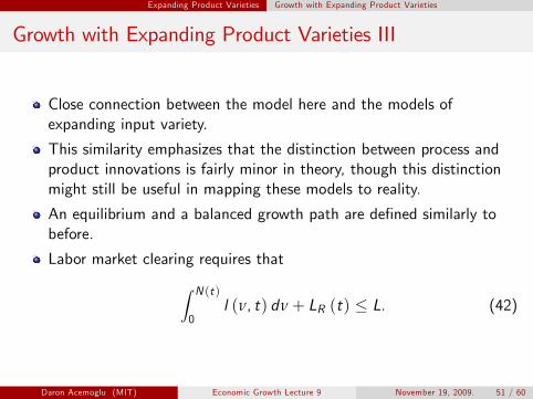
Close connection between the model here and the models of expanding input variety.
This similarity emphasizes that the distinction between process and product innovations is fairly minor in theory, though this distinction might still be useful in mapping these models to reality.
An equilibrium and a balanced growth path are defined similarly to before.
Labor market clearing requires that � N (t) l (ν, t) dν + LR (t) ≤ L. (42)
0
Daron Acemoglu (MIT) Economic Growth Lecture 9 November 19, 2009. 51 / 60
Expanding Product Varieties Growth with Expanding Product Varieties
Growth with Expanding Product Varieties IV
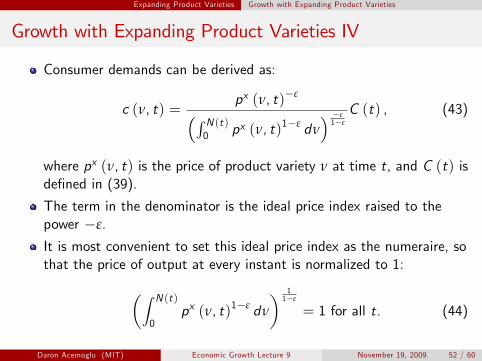
Consumer demands can be derived as:
c (ν, t) = �� N (t) p
p
x
x
(
(
ν
ν
,
,
t
t
)
)
1
−
−
ε
ε dν � 1−−
εε C (t) , (43)
0
where px (ν, t) is the price of product variety ν at time t, and C (t) is defined in (39).
The term in the denominator is the ideal price index raised to the power −ε.
It is most convenient to set this ideal price index as the numeraire, so that the price of output at every instant is normalized to 1: �� N (t)
� 1−1
ε
px (ν, t)1−ε dν = 1 for all t. (44) 0
Daron Acemoglu (MIT) Economic Growth Lecture 9 November 19, 2009. 52 / 60
Expanding Product Varieties Growth with Expanding Product Varieties
Growth with Expanding Product Varieties V
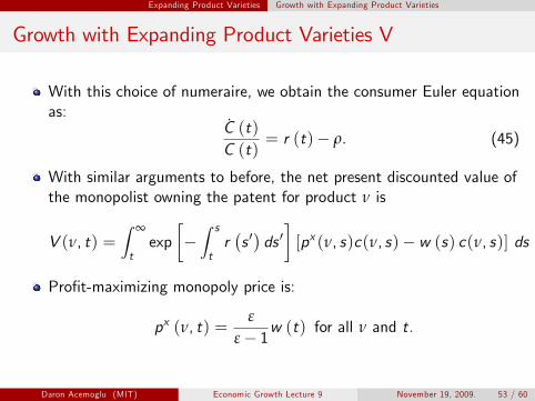
With this choice of numeraire, we obtain the consumer Euler equation as:
C (t)C (t)
= r (t) − ρ. (45)
With similar arguments to before, the net present discounted value of the monopolist owning the patent for product ν is � ∞
� � s � � �
V (ν, t) = t exp −
tr s � ds � [px (ν, s)c(ν, s) − w (s) c(ν, s)] ds
Profit-maximizing monopoly price is:
ε px (ν, t) = w (t) for all ν and t.
ε − 1
Daron Acemoglu (MIT) Economic Growth Lecture 9 November 19, 2009. 53 / 60
Expanding Product Varieties Growth with Expanding Product Varieties
Growth with Expanding Product Varieties VI
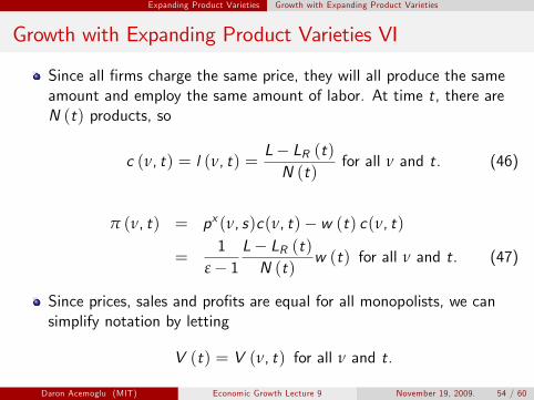
Since all firms charge the same price, they will all produce the same amount and employ the same amount of labor. At time t, there are N (t) products, so
c (ν, t) = l (ν, t) = L −NL(R
t)(t)
for all ν and t. (46)
π (ν, t) = px (ν, s)c(ν, t) − w (t) c(ν, t)
= 1 L − LR (t) w (t) for all ν and t. (47)
ε − 1 N (t)
Since prices, sales and profits are equal for all monopolists, we can simplify notation by letting
V (t) = V (ν, t) for all ν and t.
Daron Acemoglu (MIT) Economic Growth Lecture 9 November 19, 2009. 54 / 60
Expanding Product Varieties Growth with Expanding Product Varieties
Growth with Expanding Product Varieties VII
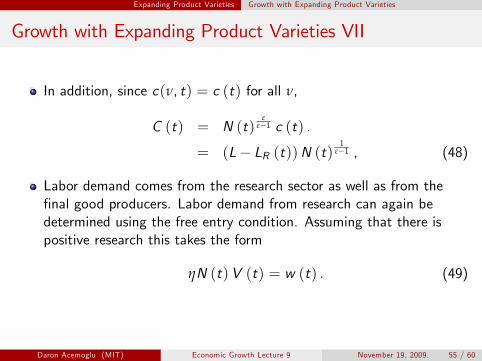
In addition, since c(ν, t) = c (t) for all ν,
ε
C (t) = N (t) ε−1 c (t) . 1
= (L − LR (t)) N (t) ε−1 , (48)
Labor demand comes from the research sector as well as from the final good producers. Labor demand from research can again be determined using the free entry condition. Assuming that there is positive research this takes the form
ηN (t) V (t) = w (t) . (49)
Daron Acemoglu (MIT) Economic Growth Lecture 9 November 19, 2009. 55 / 60
Expanding Product Varieties Growth with Expanding Product Varieties
Characterization of Equilibrium I
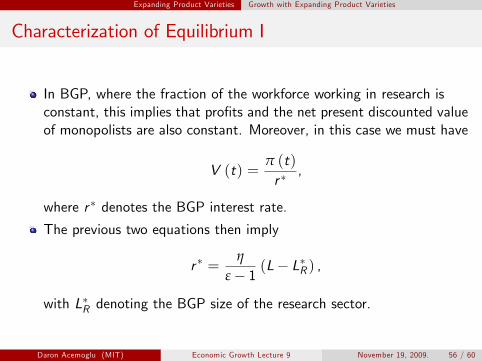
In BGP, where the fraction of the workforce working in research is constant, this implies that profits and the net present discounted value of monopolists are also constant. Moreover, in this case we must have
V (t) = π (t)
,r ∗
where r ∗ denotes the BGP interest rate.
The previous two equations then imply
η r ∗ =
ε − 1 (L − LR
∗ ) ,
with LR ∗ denoting the BGP size of the research sector.
Daron Acemoglu (MIT) Economic Growth Lecture 9 November 19, 2009. 56 / 60
Expanding Product Varieties Growth with Expanding Product Varieties
Characterization of Equilibrium II
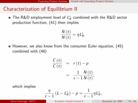
The R&D employment level of L∗ R combined with the R&D sector production function, (41) then implies
N (t)= ηL∗ R .N (t)
However, we also know from the consumer Euler equation, (45) combined with (48)
C (t) C (t)
= r (t) − ρ
1 N (t) = ,
ε − 1 N (t)
which impliesη 1
ε − 1 (L − LR
∗ ) − ρ = ε − 1
ηLR ∗ ,
Daron Acemoglu (MIT) Economic Growth Lecture 9 November 19, 2009. 57 / 60
Expanding Product Varieties Growth with Expanding Product Varieties
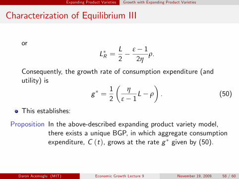
Characterization of Equilibrium III
or
LR ∗ =
L 2 −
ε 2− η 1
ρ.
Consequently, the growth rate of consumption expenditure (and utility) is � �
1 η g ∗ =
2 ε − 1L − ρ . (50)
This establishes:
Proposition In the above-described expanding product variety model, there exists a unique BGP, in which aggregate consumption expenditure, C (t), grows at the rate g ∗ given by (50).
Daron Acemoglu (MIT) Economic Growth Lecture 9 November 19, 2009. 58 / 60
1
2
3
Expanding Product Varieties Growth with Expanding Product Varieties
Discussion
Some features are worth noting:.
Growth of “real income,” even though the production function of each good remains unchanged. No transitional dynamics. Scale effect.
Hence, whether one wishes to use the expanding input variety or the expanding product model is mostly a matter of taste, and perhaps one of context.
Both models lead to a similar structure of equilibria, to similar equilibrium growth rates, and to similar welfare properties.
Daron Acemoglu (MIT) Economic Growth Lecture 9 November 19, 2009. 59 / 60
1
2
Conclusions Conclusions
Conclusions
Different models of endogenous technological progress. Key element: non-rivalry of ideas and monopolistic competition. The pace of technological progress determined by incentives
market structure, competition policy, taxes, patents and property rights
Equilibrium typically not Pareto optimal, even in the absence of distortionary policies;
because of monopolistic competition in practice, barriers to research and innovation may be more important than monopoly distortions.
A number of special features No direct competition among producers (only sometimes in the labor market). No quality differentiation.
Schumpeterian aspects of innovation and growth missing. With Schumpeterian creative destruction, monopoly and increasing returns still important, but nonrivalry of ideas will be limited.
Daron Acemoglu (MIT) Economic Growth Lecture 9 November 19, 2009. 60 / 60 Topic for next lecture.

For information about citing these materials or our Terms of Use, visit: http://ocw.mit.edu/terms.
MIT OpenCourseWare http://ocw.mit.edu
14.452 Economic Growth Fall 2009
For information about citing these materials or our Terms of Use,visit: http://ocw.mit.edu/terms.


![Energy taxes and endogenous technological change (Running ...public.econ.duke.edu/~peretto/EnergyTaxes.pdf · [10]); Barsky and Killian, in contrast, argue that they matter very little](https://img.pdfslide.us/doc/110x75/5e95217cddc9b5741668cd9f/energy-taxes-and-endogenous-technological-change-running-perettoenergytaxespdf.jpg)