1

DOES INDUSTRY SELF-REGULATION REDUCE ACCIDENTS?

RESPONSIBLE CARE IN THE CHEMICAL SECTOR

Stephen R. Finger

and

Shanti Gamper-Rabindran

Version 11/18/2011

Stephen Finger, Assistant Professor, Moore School of Business, University of South Carolina

(stephen.finger@moore.sc.edu) and Shanti Gamper-Rabindran, Assistant Professor, Graduate School of

Public and International Affairs, University of Pittsburgh (shanti@gspia.pitt.edu). Corresponding author:

S. Gamper-Rabindran. We thank Wayne Gray, John Mendeloff, participants at the Industry Studies

Association, European Association of Environmental and Resource Economists and Association of Public

Policy and Management for helpful suggestions. We gratefully acknowledge funding from the National

Science Foundation (BCS 0351058 and SES 1127223), University of Pittsburgh’s Central Research

Development Fund, University Center for Social and Urban Research, and the European Union Center of

Excellence. Errors are our own.

2

Does Self-Regulation Reduce Industrial Accidents?

Responsible Care in the Chemical Industry

Abstract

This is the first study to evaluate the impact of self-regulation on industrial accidents. We

examine Responsible Care in the US chemical manufacturing sector using our author-

constructed database of 1,867 firms that own 2,963 plants between 1988 and 2001. Firms’ self-

selection into RC is instrumented using pollution-related regulatory pressure on firms that

influences their probability of joining RC, but not plant-level accidents. The average treatment

effect on the treated indicates that RC reduces the likelihood of accidents by 2.99 accidents per

100 plants in a given year. This 69.3% reduction in the likelihood of accidents, accounting for

the plants that participate in RC, translates to back-of-the-envelope avoided losses of $0.8 billion

to $3.8 billion per year. RC also reduces the likelihood of more narrowly-defined accidents, i.e.,

process safety accidents and accidents related to violations of RC codes, by 5.75 accidents per

100 plants in a given year or by 85.9%.

150 words

Keywords: Corporate Social Responsibility, Industry Self-Regulation, Industrial Accidents,

Process Safety, Environmental and Health Safety

JEL codes: Q53 Q58 L51 L65 D21

3

1. Self-regulation and industrial accidents

Major accidents in the chemical industry – Seveso’s dioxin release, Bhopal’s methyl-

isocyanate release and the explosion at AZF Toulouse – highlight the costs from industrial

accidents (Kleindorfer and Kunreuther, 1987; Dechy et al., 2004; NCBP, 2011; Capelle-

Blanchard and Laguna, 2010). Industrial self-regulation, in which trade associations require

members to adhere to codes of conduct, has become one prominent policy response to these

accidents. In reaction to Bhopal, the American Chemistry Council (ACC) launched Responsible

Care (RC) in the US chemical manufacturing sector (Rees, 1997). Most recently, the National

Commission on the BP Oil Spill (NCBP, 2011), citing the success of RC, recommended that the

oil and gas drilling sector adopt self-regulation. In turn, the industry association is considering

establishing a self-regulation program that includes the features of RC (Dlouhy, 2011).

We examine the impact of Responsible Care, operating within its regulatory context,1 on

work-related accidents involving at least one fatality or three inpatient hospitalizations among

workers in the US chemical manufacturing sector. We analyze our author-constructed database

which consists of 2,963 plants owned by 1,867 firms between 1988 and 2001. Our study, the first

to examine the impact of industry self-regulation on industrial accidents,2 is of policy interest.

1 The chemical manufacturing sector faces regulations and costs of insuring against accidents

(Kleindorfer and Kunreuther, 1987). See section 2.1. The chemical manufacturing sector is the

Standard Industrial Classification major group 28, i.e., SIC-28. This sector is composed of

industries at the SIC-4 digit level (SIC-4) which are listed in the Online Appendix II: Table A1.

2 The seminal papers examining accidents in the Risk Management Plan database do not examine

self-regulation (Kleindorfer et al., 2003). Davis and Wolfram’s (2011) analysis of the impact of

4

First, firms are likely to under-invest in accident prevention because they are able to externalize

some of the costs from accidents (Gray and Jones, 1991; Cohen et al., 2011). Accidents in the

US chemical industry are estimated to cause losses of $3 billion to $5 billion annually (Collins et

al., 2000). Second, despite the justifications for self-regulation programs, i.e., firms, not

regulators, have the information, technology and resources for risk management (National

Academy of Engineering, 2010; GAO, 2011), empirical studies to date conclude that RC did not

reduce participants’ pollution (King and Lenox, 2000; Gamper-Rabindran and Finger, 2010).

Our study assesses RC on the yardstick of accidents. Plausibly, RC, created in response to the

Bhopal accident, focused mainly on the implementation of codes related to production safety,

instead of pollution reduction, because poor management of production processes caused that

accident (Kleindorfer and Kunreuther, 1987). Moreover, the accident outcome, due to mandatory

reporting to the Occupational Safety and Health Agency (OSHA) and follow-up investigations,

is more reliably measured than the self-reported Toxic Release Inventory (TRI) pollution

examined previously (King and Lenox, 2000; Gamper-Rabindran and Finger, 2010).

A key methodological challenge in analyzing the impact of self-regulation programs or

voluntary programs is that firms self-select into these programs based on factors that are

unobserved by the researcher, but that are likely to be correlated with the program outcomes

(Levinson, 2004). Furthermore, the direction of bias from not addressing self-selection is often

not known a priori.3 The first solution to the self-selection problem, i.e., randomizing the

deregulation on efficiency in nuclear power plants reports some evidence that deregulation

improved one measure of plant safety.

3 In his study of the voluntary program for early compliance under the Acid Rain Program,

Montero (1999) finds that plants that are able to reduce their emissions prior to the compliance

5

programs to participants and non-participants, is inappropriate because a firm’s choice to

participate is an essential feature of these programs. The second solution, i.e., instrumenting for

firm’s selection, faces the obstacle that valid instruments are available only in limited cases.4 The

criticism of identifying assumptions in several studies underscores the difficulty in proposing

valid instruments.5 Several recent studies (Pizer, Morgenstern and Shih, forthcoming; Kim and

Lyon, 2011) have relied on Propensity Score Matching methods (PSM). The authors’

date and thus, receive excess allowances based on their historical emissions are more likely to

opt into the program. In contrast, in their study of RC whose membership codes include pollution

reduction, Lenox and Nash (2003) find that more polluting firms are more likely to join RC. Not

addressing self-selection would overstate the impact of the program in reducing pollution if these

dirtier plants face lower marginal costs in reducing pollution, as a result of declining marginal

costs of abatement. The bias would be in the opposite direction if these plants face higher

marginal costs of reducing pollution as a result of their reliance on pollution-intensive

technologies.

4 Studies of the voluntary 33-50 program are able to use an instrument based on the

Environmental Protection Agency’s (EPA) invitation of firms to join the program in several

waves that are orthogonal to the program’s outcome (Khanna and Damon, 1999; Gamper-

Rabindran, 2006; Vidovic and Khanna, 2007).

5 For example, Brouhle, Griffiths and Wolverton’s (2009) study is a valuable contribution but

their assumption that several variables do not affect plants’ emissions is prone to criticism. In the

authors’ model, state regulations, prior violations and penalties, and a subset of community

pressure variables do not affect plants’ emissions, contrary to the evidence in Sigman (1999),

Gray and Shimshack (2011) and Hamilton (1995, 1999), respectively.

6

justification for applying PSM is the absence of valid instruments, but one concern is the authors

have not ruled out the potential scenario that firms’ selection into the program is based on

unobserved factors related to outcomes.6 The PSM estimates are biased when unobserved factors

influence both participation and outcomes (Heckman, Ichimura, and Todd, 1997).

To instrument for a plant’s parent firm’s participation in RC, our study exploits the firm’s

exposure to impending strict regulations on hazardous air pollutants (HAPs), which are a subset

of its TRI pollutants. Impending regulations on HAPs affect the firm’s contemporaneous

decision to join RC, but do not directly affect plant-level accidents. These anticipated Maximum

Available Control Technology (MACT) regulations reduce the additional costs for regulation-

affected plants to join RC. Firms that would have to reduce their HAPs in the future anyway may

face lower costs to adhere to RC’s pollution prevention membership code, and thus, be more

likely to participate. The impending MACT regulations are not likely to affect accidents (section

3.3). First, technologies to reduce HAPs released into the environment, e.g., improved

incineration or chemical absorption of HAPs (Van Asten and Martinson, 2005), are distinct from

6 In the 1605b program, which provides project-level reporting options, it is plausible that firms

which are already planning a sequestering project are more likely to self-select into the program.

These firms are also less likely to undertake actions to reduce the two outcomes analyzed: (i)

energy usage examined in Pizer, Morgenstern and Shih (forthcoming); and (ii) carbon dioxide

emissions intensity examined in Lyon and Kim (2011). As firms’ planned sequestration project is

not observed by researchers, matching such firms (which have a planned sequestration project)

with other firms that are similar in their observables (but which do not have a planned

sequestration project) can bias the studies towards finding that the program did not reduce energy

usage or emissions intensity.

7

actions to reduce plant-level accidents, e.g., preventing pressure buildup, loss of control over

reactive processes or exposure of flammable chemicals to heat sources (Hofman, Jacobs and

Landy, 1995). Second, EPA’s design and implementation of MACT regulations did not consider

potential impacts on worker exposure or accidents (Armenti et al., 2003; Armenti, 2004; Robson

and Toscano, 2007). Third, even if MACT regulations had reduced HAPs, these reductions are

not likely to result in fewer accidents. Many accidents stem from fires, explosions, or acute

worker exposure to toxic chemicals, but few HAPs are flammable or acutely toxic. The reduction

of HAPs that are carcinogenic or chronically toxic are not likely to reduce deaths or

hospitalizations because of the long latency periods between chronic exposure and symptoms of

illness (Robson and Toscano, 2007).

We find that RC reduces the likelihood of all accidents at RC participating plants by 2.99

accidents per 100 plants for a given year. This figure is the estimated treatment effect on the

treated. Based on estimates of losses from accidents at chemical, petrochemical or OSHA-

regulated plants, and the 1,037 average number of plants that participate in RC, this 69.3%

reduction in the likelihood of accidents translates to back-of-the-envelope avoided losses of $0.8

billion to $3.8 billion annually (see section 4.4). Narrowing our analysis to process safety7

accidents and those accidents involving violations of OSHA standards related to RC codes, we

find that RC reduces the likelihood of these accidents by 5.75 accidents per 100 plants in a given

year, or by 85.9%.

7 Process safety denotes the application of management and engineering principles to prevent

fires, explosions, and accidental chemical releases at chemical plants (ACC, 1990). It is often not

possible to stop a process that is going out of control by simply “pulling the plug” and stopping

the production line (Hofman, Jacobs and Landy, 1995).

8

Our results yield two policy implications. First, RC provides additional impetus for plants

to improve their safety standards, beyond the incentives they face from government regulations

and their potential liability from accidents. RC features can improve senior management’s

attention to safety and their ability to correct errors, the two key factors in improving plant safety

(section 2.2). These features include requiring CEOs of firms to sign off on reports to the ACC,

to attend regional meetings where they are subject to peer pressure to improve their firms’ safety

record, and in requiring plants to conduct safety audits. Top management’s commitment to safety

can translate into improvements down the production chain, given workers’ self-interest in

improved safety.

The second policy implication is that the underlying regulatory framework sets the

incentives that determine whether self-regulation programs attain their stated goals. Thus, self-

regulation programs are best treated as complements to regulation. Our results, that RC reduced

accidents, stand in contrast to the results from previous studies, that RC or other voluntary

programs did not reduce TRI pollution significantly (King and Lenox, 2000; Morgenstern and

Pizer, 2007; Gamper-Rabindran and Finger, 2010). Despite RC’s stated goals to reduce both

accidents and pollution, RC plants, on average, reduce their accidents but not their TRI pollution.

This is because the regulatory framework yields greater net benefits from reducing the likelihood

of accidents, e.g., reduced insurance and expected liability costs, than from reducing their TRI

pollutants, some of which are unregulated (section 5).

2. Responsible Care and industrial accidents

2.1 Self-regulation

Self-regulation programs operate within a framework of regulations and liability.

Chemical plants are subject to the 1992 OSHA Process Safety Management (PSM) rules, which

9

set requirements for management processes when using highly hazardous chemicals, and the

1996 Environmental Protection Agency (EPA) Risk Management Program (RMP), which

require plants with specific chemicals to undertake accident prevention programs. Plants are also

subject to worker compensation laws, which hold employers liable for work-related deaths and

injuries (Kleindorfer et al., 2003).

In response to the Bhopal and Three Mile Island accidents, the chemical and nuclear

sectors launched self-regulation programs, i.e., RC and the Institute of Nuclear Power

Operations, respectively (Rees, 1994; Rees, 1997). By restricting their membership to those

firms that commit to adhere to codes of conduct, the self-regulation program can potentially

distinguish purportedly lower risk firms (members) from purportedly higher risk firms (non-

members). The self-regulation program, however, faces a collective action problem among

members. While all members would benefit if the self-regulation program successfully achieves

its stated goals of risk reduction, each member has an incentive to free ride, i.e., join the program

but not comply with the codes. The trade association’s inability to impose sanctions constrains

its ability to limit free-riding (Lyon and Maxwell, 2004; Prakash and Potoski, 2007; Barnett and

King, 2008).

Whether self-regulation programs successfully reduce risk is debated. On the one hand,

industries have a strong motivation to succeed in self-regulation. These programs can potentially

forestall the state’s imposition of stricter and more costly regulations (Maxwell et al., 2000).

Dawson and Segerson’s (2008) theoretical study notes that as long as a subset of firms comply

with their commitments, even if other firms free-ride, the self-regulation program can achieve its

goals. The compliers are those firms which would face significant costs from more stringent

regulation should the self-regulation program fail. On the other hand, Glachant’s (2007)

10

theoretical study suggests that in some cases, firms enter self-regulation programs without any

intention to comply with their commitments, and then lobby for the weakening of the final

legislation. Firms are able to not comply with their commitments because their non-compliance

is not immediately observable.

2.2 Responsible Care and potential improvements to participants’ safety culture

The two major factors that influence plants’ safety are: (1) the senior management’s

commitment to safety (Pidgeon and O’Leary 2000, Krause, 2004); and (2) the ability of the

management and the organization to learn from errors (Reason, 1997, cited in CSB-Texas City,

2007). Further details on the role of top management in plant safety are in the Online Appendix

I. Regulations, such as the PSM and RMP rules, and liability in the case of accidents, provide

incentives for top management to ensure a basic level of plant safety. RC imposes additional

requirements that would bring the plants’ safety records to the attention of top management and

encourage improvements of their plants’ safety.

Chief Executive Officers (CEOs) must sign off on annual reports submitted to the ACC

on their firms’ environmental health and safety performance (Yosie, 2003). In the absence of the

RC requirements, plants must still report their accidents to OSHA, but there is no mechanism to

ensure that senior management is made aware of their plants’ safety records. CEOs also face peer

pressure, which can potentially influence their adherence to RC membership codes. According to

the NCBP (2011), “[RC’s] success has turned less on the availability of such formal sanctions

and more on informal disciplinary mechanisms such as peer pressure and institutional norms of

compliance: ‘Executives from leading firms pressure their non-compliant counterparts at

industry meetings to adopt and adhere to the industrial codes.’” RC’s codes include the

Environmental Health and Safety (EHS), Process Safety (PS) and Community Awareness and

11

Emergency Response (CAER) codes (ACC, 1990).8 These codes promote risk management in

the production process, e.g., improving management of pressure or heat-related processes,

improving management of flammable, reactive or corrosive chemicals, and minimizing workers’

exposure to chemicals (Spellman, 1997).

RC participants must perform self-audits on their safety performance, which can uncover

shortcomings in their safety systems. For example, RC requires self-audits of the Process Safety

Code. “The code requires companies to have management practices in place to ensure, among

other items—periodic assessment and documentation of process hazards, complete

documentation on the hazards of materials, and sufficient layers of protection to prevent a single

failure from leading to a catastrophic event” (CSB-First Chemical Corp, 2003). These RC

features can serve the function of “attention correction,” a term used by Scholz and Gray (1990)

to describe the effect of bringing safety shortcomings to the attention of management. Top

management’s attention to safety can then translate into improvements down the production

chain, given workers’ self-interest in improved safety.

Ultimately, whether the RC program has reduced the likelihood of accidents is an

empirical question. While RC features can potentially improve safety, the pre-2002 RC program

may not provide sufficient incentives for plants to truly implement safety improvements. In

particular, pre-2002, the ACC did not have a mechanism to verify plants’ safety reports or to

verify that plants corrected safety hazards uncovered during self-audits.9 While the RC program

8 Details of RC’s codes and management practices are described in ACC (1990).

9 There are cases in which RC participating plants are made aware of defects in their process

hazard analysis, but failed to correct those defects. For example, from OSHA’s inspection and

citation, Bayer CropScience learned that their process hazard analysis was defective, but the

12

did introduce third party certification in 2002, our study of the pre-2002 RC program, without

third party verification, is of policy interest, because other programs share this characteristic and

several industrial sectors lack independent third party certifiers (O’Rourke, 2003; Rosenthal and

Kunreuther, 2010).10

3. Research questions and data

We test if RC, operating within its regulatory framework, reduced OSHA-reportable

accidents. RC and the underlying regulatory and insurance institutions are interactive in their

effects. Therefore, we provide an estimate of the impact of RC, given the underlying institutional

framework, versus non-participation in the same framework. This estimate remains informative

for self-regulation programs operating in comparable institutional settings.

Our sample of 23,780 plant-years in the chemical manufacturing sector (SIC-28) between

1988 and 2001 consists of 2,963 plants owned by 1,867 firms. This sample consists of SIC-28

plants which we have successfully linked across three databases and fulfill three conditions: they

(i) report their pollution to the TRI, (ii) report their number of employees to Dun & Bradstreet

(D&B) and (iii) are inspected at least once by OSHA between 1984 and 2009. Our TRI-D&B

sample contains SIC-28 plants linked across these two databases. Our OSHA sample is derived

from inspection reports for SIC-28 plants in the OSHA Integrated Management Information

plant failed to fully implement corrective actions. Because their process hazard analysis

remained defective, safety hazards were not identified and corrected, and those hazards

contributed to a subsequent accident at the plant (CSB-Bayer CropScience, 2011).

10 In 2002, with the launch of RC14001, the ACC required third-party verification of plants’

conformance to the RC14001 technical standards (Moffet et al., 2004).

13

System (IMIS) database. 11 These reports are then matched by plant names, addresses, and SIC-4

code to generate plants’ inspection histories. Using Fellegi and Sunter’s (1969) matching

techniques, we link the TRI-D&B sample with the OSHA sample using plants’ names, addresses,

geocoded locations and SIC-4 code.12 Data on accidents is from the IMIS Fatality and

Catastrophe Investigation Summaries data (OSHA form 170), also known as the Accident

Investigation Summaries (AIS) database. Data on inspections, violations detected during

inspections, and related penalties are from the IMIS Inspection database. Data on hazardous air

pollutants are from the TRI. Pollutants are restricted to those chemicals reportable since 1987 to

the TRI. Tract-level neighborhood demographics are from the Decennial Census, and SIC-4

industry variables are from the Bureau of Economic Analysis. We create annual plant-firm

linkages using Mergent Online and Corporate Affiliations Database.

3.1 Accidents

OSHA mandates employers to contact OSHA within eight hours if a work-related

accident occurs, i.e., at least one fatality occurs or at least three workers require inpatient

hospitalization13 (CPL 02-00-113 (2.113)). With minor exceptions, reporting to the AIS is

11 Plant-level details are recorded in the IMIS database only if they have been inspected at least

once. Weil (1996) uses a similar restriction in his analysis of OSHA plants.

12 The matching is implemented using FEBRL software (Christen, 2008). The algorithm provides

an indication of the quality of the match between plants from the two separate databases. For

matches that are border-line in quality, we undertake further library research to determine if there

is a true match.

13 This definition excludes offsite motor vehicle accidents, heart attacks that are not work-

related, and homicides at the workplace. Prior to 1994 employers had 48 hours to report and the

14

consistent over time and covers the 29 states where the Federal agency implements OSHA

programs, and the rest of the states that are authorized to implement OSHA programs. The AIS

spans the years 1984 to 2005. On notification of accidents, OSHA investigates those accidents

that are potentially related to violations of OSHA standards and OSHA inspectors issue citations

on the confirmed violations (Mendeloff and Kagey, 1990). The AIS data has been found to be

reliable; 85% of the fatalities that should be reported to OSHA are in fact being reported and

inspections were at least planned for all the fatalities that should unambiguously be inspected

(Safety Sciences, 1977, cited in Mendeloff and Kagey, 1990). We do not use the RMP accident

database because its first reported accident is in 1994, i.e., 5 years after the start of the RC

program (Kleindorfer et al., 2007).

We use three different definitions for accidents, all outcome variables are binary. Our

first and broadest definition of accidents is the occurrence of an OSHA-reportable accident as

recorded in the AIS for a plant-year. Our second narrower definition, RC or Process Safety

(RC/PS) accidents, includes: (i) accidents related to violations of RC-related codes or (ii) process

safety accidents, or both. For each accident, we code whether the investigation has cited at least

one violation of OSHA standards related to RC codes. One may surmise that these accidents

occur, in part due to these violations, because accident investigations focus on the causes of

accidents and cite violations uncovered during the inspections.14 For each accident, we also code

whether it is a process safety accident, i.e., accidents that stem from chemical leaks, high

threshold for reporting had been 5 inpatient hospitalization instead of 3 (29 CFR 1904.8. 1993

edition and 1994 edition).

14 This is an imperfect measure of accidents related to the violations of RC codes because all

violations observed during inspections, including those unrelated to the accident, must be cited.

15

pressure, fires, or explosions, according to OSHA accident investigation summaries.15 Process-

safety accidents are difficult to contain and may turn catastrophic (Hofmann, Jacobs, Landy,

1995). Because attention to routine injuries can deflect attention away from underlying process

safety issues (NCBP, 2011; Baker report, 2007, Elliott et al. 2008), we exclude “routine”

injuries, unrelated to RC codes, that affect only a few workers in a given accident, such as

injuries from falling objects or limbs being caught in machinery. Our third definition, restricted

to accidents involving fatalities, captures the most severe incidents.

In our sample of 23,780 plant-years, we observe 304 accidents, and about two thirds of

these are RC/PS accidents and about one third are fatal.16 It is rare for a plant to experience more

than one accident in a given year,17 therefore, treating the accident outcome as a binary variable

is appropriate. It is also rare for a plant to experience a large number of accidents in the entire

sample period. Of the 304 accidents, 65.8% occur at plants with only one accident and 88.8%

15 We code as process safety accidents, those accidents: (i) that involve chemical reactions,

flammable liquids, over or under-pressure, gas, vapor, mist, fumes or smoke, or (ii) in which

fatalities or injuries are related to chemical burns, heat burn, scalding or poisoning. We also

include fatalities and injuries related to electrical shock because poor electrical design can

contribute to larger scale accidents.

16 The number of accidents, RC/PS accidents and fatal accidents are 126, 94 and 45 in RC plants;

and 178, 118 and 65 in non-RC plants.

17 Out of the 304 cases of all accidents, only 11 plants had two accidents and one plant had three

accidents in the same year. Out of the 212 cases of RC/PS accidents, only five plants had two

accidents and one plant had three accidents in the same year. Of the 110 fatal accidents, only one

plant had two accidents in the same year.

16

occur at plants with two or fewer accidents between 1988 and 2001. Of the 212 RC-related

accidents, 76.4% occur at plants with one accident and 93.4% occur at plants that have two or

fewer accidents in the study period. Of the 110 fatal accidents, 90.1% occur at plants with only

one accident during the study period.

3.2 Estimation model

Our estimation model for the impact of RC on accidents is:

Plant hazard level (accident outcome) Y it = 1 [Rit β1 + Xit β2 > νit ] Equation 1

Participation in RC R it = 1 [Zit α1 + Xit α2 > εit ] Equation 2

εit , νit ~ N (0, Σ)

where observations are for plant i in year t, the dependent variable, Y is a dummy variable for the

occurrence of at least one accident during a plant-year, R is a dummy indicating the plant’s

parent firm’s participation in RC, X are covariates, and νit and εit are the error terms. Z, the

instrumental variable, captures the plant’s parent firm’s exposure to impending MACT

regulations, as measured by the firm’s share of pollution released into the environment that are

HAPs (section 3.3).

We employ a bivariate probit model (Heckman, 1978) in which the outcome (the

occurrence of an accident) and the treatment (RC participation) are each determined by latent

linear index models with jointly normal error terms. This specification maps directly to two

interrelated decision-making processes: (i) the decision to join RC by the plant’s parent firm, as a

function of covariates and the error term, εit, with that firm joining RC if its net benefits of

joining exceed a threshold, and; (ii) the occurrence of accidents at a plant as a function of the

observed covariates and an unobserved hazard shock, νit, with accidents occurring if the

17

combined hazard level and shock at the plant exceed a threshold. The terms νit and εit may be

correlated as unobserved factors, known by the firm, and may both affect the firm’s decision to

join RC and be related to the hazard level at the plant.18 The bivariate probit corrects for firm’s

self-selection into RC based on unobserved factors and is correctly specified for a model with an

endogenous dummy variable, i.e., the RC participation dummy. As described in section 4.2, we

find significant correlation between the errors in the RC participation equation and the errors in

the accident equation; therefore, our final estimation model must address self-selection.

The bivariate probit is our preferred specification, given the nature of our accident data.

The mean likelihood of accidents in our sample period is low, amounting to only 1.28%. The

linear IV does not impose that the predicted probabilities implied by the model range between 0

and 1. This problem is especially severe when the mean of the main outcome is close to either 0

or 1; therefore, the linear IV should not be used when the average probability of the dependent

variable is not near 0 or 1 (Bhattacharya, Goldman, and McCaffrey, 2006). Indeed, we find that

one third of the predicted probabilities from the linear IV estimated for our accidents data lie

outside the [0,1] range.

The bivariate probit requires that both error terms are distributed bivariate normal for

estimates to be unbiased (Angrist, 1999). Its identification relies on both the instrument and the

functional form (Altonji, Elder and Taber, 2005). The bivariate probit remains our preferred

specification because it may be less biased than the linear IV, even when the errors are non-

normal (Bhattacharya, Goldman, and McCaffrey, 2006). In simulations with non-normal errors

18 Alternatively, the firm may first observe the level of hazard at its plants, and then, make its

decision on participating in RC. The key estimation issue is that the bivariate probit can address

the firm’s self-selection into RC based on factors unobserved by the researcher.

18

the bivariate probit leads to a smaller level of bias over various parameter configurations

compared to Linear Probability Model (LPM), often with the smaller variance as well. The

authors report that, “[the bivariate probit] nearly always, though not always, performs better than

the LPM estimator.”19 We report bootstrap standard errors with 100 replications for the bivariate

probit, as recommended by Chiburis, Das and Lokhsin (2011). This strategy addresses the

concern that misspecification in the bivariate probit may lead to the underestimation of the

standard errors.

3.3 Instrumental variable to address firms’ self-selection into RC

As an instrumental variable for a plant’s parent firm’s participation in RC, we use the

firm’s share of pollution released into the environment that are hazardous air pollutants (HAPs).

The instrument, the firm’s HAP/TRI ratio, is defined as the ratio of HAPs emissions (as reported

to the TRI) to total TRI air emissions for all plants owned by the firm. We argue that the firm’s

HAP/TRI ratio influences its contemporaneous decision to participate in RC, but does not

directly affect plant-level accidents, conditional on their other included characteristics, such as

plants’ TRI emissions-intensity relative to their SIC-4 and the average TRI emissions-intensity in

their SIC-4 relative to the chemical industry as a whole.

During our study period, plants in the chemical manufacturing sector face strict

regulations on their emissions of HAPs with expected implementation dates in the late 1990s.

19 Simulations by Chiburis, Das and Lokshin (2011), reported in their Figure 5, indicate that for

low probabilities such as 0.1, the bias is less for the bivariate probit than the linear IV. In related

work, Horrace and Oaxaca (2003) conclude that even with a linear data generating process, the

probit leads to lower mean squared errors than OLS, and the difference is largest when

conditional probabilities are extreme.

19

The Clean Air Act requires the EPA to set MACT standards on plants that emit HAPs. MACT

standards require existing and new chemical plants to install the technology that has been

adopted by plants in the same production category that have achieved the best pollution control

and the lowest pollution emissions (Solomon and Han, 2007). Firms whose plants have large

shares of HAPs would have to reduce these plants’ emissions in the future in response to the

impending MACT standards, and would have to do so even in the absence of the RC program.

Thus, these firms face little additional costs to meet RC’s pollution prevention code, and are

more likely, on average, to decide to join RC anyway to benefit from RC’s positive publicity.

The instrumental variable, HAP/TRI ratio, is not likely to affect accidents, conditional on

the included measures of TRI emissions-intensity. First, control technologies implemented to

reduce HAPs emissions into the environment are distinct from actions undertaken to improve

plant safety. MACT regulations set stricter emissions limit for HAPs emitted from process

vents, storage tanks, wastewater streams, and equipment leaks. 20 Plants install control devices,

such as thermal or catalytic oxidizers, which burn off a greater fraction of HAPs in air streams at

high temperatures, or chemical absorbers, which absorb a greater fraction of HAPs prior to the

release of the air streams into the environment (Van Asten and Martinson, 2005). In contrast,

steps undertaken to improve safety include identifying and preventing excessive built-up of

20 For example, the Miscellaneous Organic National Emission Standards for Hazardous Air

Pollutants raised the requirement to controlling 95% of the HAP emissions from storage tanks

(Van Asten and Martinson, 2005).

20

pressure in chemical processes, the loss of control of heat-related or reactive processes, or

exposure of flammable liquids to ignition sources (Spellman, 1997).21

Second, during our study period, regulations aimed at reducing emissions to the

environment do not account for workers’ exposure to hazards.22 Adam Finkel, Director of Health

Standards Programs at OSHA between 1998 and 2003, notes that efforts to reduce stack

emissions often do not account for worker exposure.23 As of 2004, “there was no formal

consideration of the overlap between environmental and occupational exposures (outside versus

inside the plant) and the potential of pollution prevention strategies for addressing both”

(Armenti, 2004). This disconnection stems from the distinct regulatory framework separating the

EPA and OSHA and the agencies’ lack of coordination (Armenti et al., 2003).24 Gillen (2000),

21We also discussed the distinction between actions for reducing MACTs and actions for

reducing plant accidents with Jeffrey Siirola, formerly with Eastman Chemical Company,

Distinguished Service Professor, Carnegie Mellon University, pers. comm. with Shanti Gamper-

Rabindran. 26 October 2011.

22 OSHA’s and EPA’s interagency committees coordinate their interactions in other areas, such

as their activities under EPA’s RMP and OSHA’s Process Safety Management.

23 Dr. Adam Finkel in phone conversation with Shanti Gamper-Rabindran, 15 January 2011.

24 Regulations curbing industry’s emissions of HAPs to the environment, due to the failure to

consider effects on worker safety, can even worsen workers’ exposure. In one example, to

improve air quality standards, the California Air Resources Board decided in 1997 to phase out

chlorinated solvents used in the auto repair industry; unfortunately, that policy inadvertently

contributed to the overexposure of workers to the substitute chemical hexane which caused

peripheral neuropathy (Wilson et al, 2007).

21

from the EPA Office of Pollution Prevention and Toxics, reports that as of 2000, “pollution

prevention strategies have not typically included the additional step of coordinating on worker

health issues.”

Third, even if impending MACT regulations led plants to reduce their HAPs, that

reduction would not translate to significant reductions in accidents. Many accidents stem from

fires, explosions, or acute worker exposure to toxic chemicals, but only a small proportion of

HAPs are flammable or acutely toxic. Out of 19025 HAPs, six are flammable and 26 are acutely

toxic. Also, the reduction of HAPs that are carcinogenic or chronically toxic is not likely to

reduce deaths or hospitalizations in the short-term because of the long latency period between the

chronic exposure to chemicals and the onset of major symptoms (Robson and Toscano, 2007). In

our accidents database, most cases of deaths or hospitalizations due to chemical exposure occur

as a result of chemical spills that resulted in chemical burns. Finally, there is little evidence of a

link - whether none, positive, or negative - between pollution reduction strategies in production

processes and occupational hazards (Sivin, 2002). Indeed, a case study documents that the

alteration to the production method in order to eliminate the release of pollutants into the

environment inadvertently led to an increase in workers’ exposure (Sivin, 2002). Additional case

studies, presented at an OSHA-EPA conference, indicate that plants complied with emissions

limitations from point sources by increasing the fraction of a toxic pollutant that remains in the

workplace (Robson and Toscano, 2007).

We have also investigated the possibility that the MACT requirements may have led to

plants changing their processes to reduce both HAPs and accidents. Our conversations with the

25 The top chemicals associated with RMP accidents are ammonia (non-HAP), chlorine (HAP)

and flammable mixtures (Kleindorfer et al., 2003).

22

industry and the EPA have not yielded evidence for this scenario. Finally, our excluded variable

would not be invalidated if after our study period, MACT regulations affect occupational

hazards, whether positively or negatively. Interestingly, significant coordination between policies

on emissions to the environment and workers’ exposure does not occur even three years after the

end of our study period (Armenti, 2004).

We specify the instrument as a firm’s HAP/TRI ratio to better capture its exposure to

impending MACT regulations. The alternative specification of the instrument as a firm’s total

HAPs is prone to the criticism that total HAPs may be more highly correlated to our included

TRI emissions-intensity variables, and therefore, less highly correlated with MACT regulations,

conditional on the included TRI emissions-intensity variables. Our main analysis uses total

pounds to aggregate HAPs and TRI because the MACT regulations focus on reducing the pounds

of HAPs released into the environment.26

3.4 Covariates

Our accident regressions control for regulatory variables, i.e., OSHA inspections and

penalties. For our study to be valid, we need to control for the association between

inspections/penalties and accidents, but we do not need to isolate the causal effect of

inspections/penalties on accidents. A positive association between inspections/penalties and

accidents could arise from OSHA’s targeting of inspections to plants, firms, and SIC-4 industries

26 As an alternative specification for the instrument, we weight HAP and TRI values by their

toxicity-weights as reported in the Risk Screening Environmental Indicators (RSEI) model (EPA,

2010). Results are in the Online Appendix IV: Table A3.

23

that have lower safety levels and therefore a higher likelihood of accidents27 (Tai, 2000).

Conversely, a negative association between accidents and inspections/penalties could stem from

the potential for inspections and penalties to raise plants’ safety levels (Scholz and Gray, 1990;

Gray and Scholz, 1993) and thus reduce their likelihood of accidents. We control for inspections

and penalties in the previous year and those accumulated in the prior two to five years because

enforcement requires time to produce their full effect (Scholz and Gray, 1990). We include

inspections and penalties at the firm’s plants, the SIC-4 industry and the state to account for the

general deterrence effect of inspections (Gray and Mendeloff, 2005). A dummy is included for

plants located in the 29 states where the Federal agency implements the OSHA program (Gray

and Mendeloff, 2005).

Higher premiums for worker compensation insurance can influence the firms’ safety

level; 28 but firm-level insurance data is not publicly available. Larger firms pay insurance

premiums that reflect their previous safety record; while smaller plants pay premiums that are the

same for all firms in the same industry-occupation category (Ruser, 1985). To proxy for the

variation in insurance premiums, we use: (i) the number of average employees in a firm’s plants,

a dummy for single-plant firms, and the number of plants owned by the firm to capture firm size;

27 A subset of OSHA’s inspections target plants, firms, and industries with poorer safety records;

while another subset, i.e., programmed inspections, are undertaken randomly within state-

industry cells (Gray and Mendeloff, 2005).

28 State worker compensation laws make employers liable for all of an injured worker's medical

expenses and a portion of lost wages. Except for the largest firms which self-insure, employers

are required to purchase insurance to cover their potential liabilities (Ruser, 1985).

24

(ii) the dollar penalty accrued in the past 5 years to provide a measure of the firm’s safety record;

and; (iii) SIC-4 industry dummies.

We control for plant size using the log of plant-level number of employees. We also

control for a plant’s union status29 and the share of the unionized plants among the plants owned

by the parent firm. Again the validity of our study requires our regression to simply control for

the association between unions and accidents. A negative association between unions and

accidents can arise if unions improve plant safety, e.g., by providing union members with greater

information about occupational risks, and a mechanism for voicing their concerns over this risk

(Sandy and Elliott, 1996), or by engaging in collective bargaining with management (Bacow,

1980). Conversely, union status and accidents can be positively related if workers in plants with

greater inherent hazards are more likely to unionize, or if workers in unionized plants are more

likely to be hospitalized for reporting reasons (Sandy and Elliott, 1996). Injured workers in

unionized plants may feel protected by the union, and are more able to insist on receiving

inpatient hospitalization, thus, triggering the threshold of three in-patient hospitalizations for

OSHA reportable accidents.

We control imperfectly for the inherent hazards of the SIC-4 industry and the plants in

two ways.30 First, we include SIC-4 dummy variables and year dummies to control for industry-

29 The IMIS database provides the information on a plant’s union status in the most recent

inspection year.

30 We do not use the RMP data on hazardous chemicals stored on site because (1) that data is not

available before 1999, and (2) we suspect minimal overlap between our chemical database and

the RMP. Elliott et al. (2008) link only 228 chemical plants out of the 15,219 RMP plants to

OSHA’s Occupational Injury and Illnesses database.

25

specific production technologies, which influence both the inherent hazards of the industry and

the costs of adopting safety measures (Mendeloff and Gray, 2005). Second, we control for the

pollution intensity of the plant relative to other plants operating in the same SIC-4 industry. A

plant’s pollution intensity is measured as the ratio of its toxicity weighted TRI air pollution to its

number of employees.31 Time dummies account for time variations, including changes in the

reporting threshold of five accidents to three accidents in 1994, as well as changes in production

technologies over time that influence the inherent hazards of processes and the costs of safety

precautions. The socioeconomic characteristics of a plant’s neighborhood captures the

community pressure on plants to reduce their hazard level (Hamilton, 1995; Elliott et al., 2004),

particularly, risks of chemical release, fires, or explosions that can endanger surrounding

communities. Neighborhood characteristics include the shares of whites, poor people, and non-

high school graduates at the tract-level. Kleindorfer et al.’s (2004) multi-sector study reports that

a firm’s greater financial resources are associated with fewer RMP accidents. For a given plant,

we control imperfectly for its parent firm’s resources using the log of a firm’s total employees at

its plants, a dummy for a single-plant firm, and the log of the number of plants owned by a firm.

These measures that are relative to firms’ size can, however, influence accidents through the

alternative mechanisms described above. We choose not to link to financial variables because

our study will face significant reductions in sample size, making inference impossible.32

31 Gamper-Rabindran and Finger’s (2010) analysis of SIC-4 industry level data show that, in

measuring pollution intensity, plant-level employees serve as a good proxy for output. For the

chemical sector, most of their TRI pollution releases are to air.

32 Kleindorfer et al. (2004) linked the RMP to the financial variables, which reduced their sample

size from 15,219 plants to only 2,025 plants in all sectors.

26

4. Results

4.1 Summary statistics

In our unbalanced panel data between 1988 and 2001, there are 228 RC-participating

firms that own 1,037 plants; and 1,735 non-RC firms that own 2,293 plants. Over time, few

plants change their RC status; therefore, our identification relies on the cross-sectional variation

in the data. The probability of participation in RC with covariates set at the sample means is

16.1% for all plants. Comparison of Table 1, columns 1 and 2 indicate several similarities and

differences across RC and non-RC plants; therefore, we include a full set of control variables in

our regression analysis. On average RC plants face greater likelihood of all accidents, RC/PS

accidents and fatal accidents (1.59, 1.19 and 0.57 accidents per 100 plants, respectively) than do

non-RC plants (1.12, 0.74 and 0.41 accidents per 100 plants, respectively). The greater

likelihood of accidents on average for RC plants is partly explained by RC plants’ larger average

size (measured in number of employees) and their parent firms’ larger average size (measured in

mean number of employees at firms’ plants and the number of plants belonging to firms). These

factors are associated with greater likelihood of all accidents or RC/PS accidents (Table 4). RC

and non-RC plants have a fairly similar probability of being inspected (12% versus 11%) and the

composition of their inspections is fairly similar. However, shares of inspections that lead to

violations or penalties are smaller among RC plants than non-RC plants. For inspections that do

lead to penalties, RC plants at the highest percentiles of penalties receive much larger penalties

than the corresponding non-RC plants. This small subset of RC plants drives the observation in

Table 1 that the average penalty for RC plants is much greater than that for non-RC plants. On

closer examination, penalties for most RC plants are only slightly larger than non-RC plants,

27

e.g., penalties for RC plants at the 25th, median and 75th percentiles of penalties, are only 30%,

25% and 36% greater than those for corresponding non-RC plants, respectively.

Our database represents the larger plants in SIC-28.33 We have successfully matched

IMIS inspection data to 2,421 of the 3,253 TRI-D&B plants (74.4%), analyzed in Gamper-

Rabindran and Finger (2010). Comparison of our sample of linked plants (Table 1, column 1)

and SIC-28 OSHA plants that are not linked to our data (Table 1, column 5) indicate that, while

we have only matched 25% of the IMIS data to our database, our final database is fairly

representative of plants in the chemical sector in their compliance characteristics. The linked

sample and the non-linked sample have similar shares of inspections that result in violations, and

the counts of violations conditional on non-zero violations. While the mean penalty conditional

on non-zero penalty is larger in the linked sample than in the unlinked sample, the median

penalty conditional on non-zero penalty, a measure which is less prone to outliers, is fairly

similar in the two samples.

4.2 Preliminary regressions

We estimate a probit model of plant’s RC participation on firms’ HAP/TRI ratio and a

full set of covariates. These covariates are the same as those in the accidents regression. Details

of the model are in the Online Appendix II: Table A1. We find that a plant’s parent firm’s

HAP/TRI ratio is positively associated with the plant’s parent firm’s participation in RC. The

estimated HAP/TRI coefficient of 0.342 is statistically significant at the 1% level. This result

corresponds with our hypothesis that firms with large HAP/TRI ratios anticipate having to

33 Our plants exceed the reporting threshold for emissions in the TRI. The reporting threshold for

number of employees in IMIS is 11 or more employees. The D&B database tends to include

plants with larger numbers of employees.

28

reduce pollution under the MACT regulations; and because they would have to reduce their

emissions regardless of RC, they face little additional costs in meeting RC’s pollution prevention

code, and are thus, more likely to join RC. While no tests can positively determine that an

instrument is valid, we check if the instrument is conclusively invalid. The Likelihood Ratio

(LR) test, which compares the fit of models with and without the excluded variable, rejects the

null that the firm’s HAP/TRI ratio has no effect on the probability of a plant being a member of

RC. The LR test p-value is less than 0.001. Diagnostic tests for weak instruments are not

available for the probit model (Nicholl, 2011).

Next, we estimate three specifications on RC’s association with accidents, i.e., the probit,

bivariate probit, and linear IV models (Table 2). Using the bivariate probit, we test for the

exogeneity of RC in relation to the outcome of accidents. The estimated correlation coefficient,

rho, is positive and significant at the 10% level for all accidents, significant at the 5% level for

PS/RC accidents, and insignificant for fatal accidents (Table 2, panel B). The positive rho

indicates that plants that are more likely to have accidents are also more likely to join RC.

We compare the coefficients on the RC participation dummy from the bivariate probit

models, which address self-selection (Table 2, panel B), and from the probit models, which does

not address self-selection (Table 2, panel A). This comparison indicates that when self-selection

is addressed, we find a greater impact of RC at reducing the likelihood of accidents. While the

coefficients from both types of models are negative, those from the bivariate probit models are

larger in magnitude. The coefficients for the bivariate probit are statistically significant for both

all accidents and RC/PS accidents; while those for the probit are statistically significant for all

accidents only. This pattern of plants with greater likelihood of accidents self-selecting into RC

29

is similar to the pattern of more polluting plants self-selecting into RC, detected in Gamper-

Rabindran and Finger (2010).

The linear IV (Table 2, panel C), which is inappropriate for reasons outlined in section

3.2, yields coefficients that are smaller in magnitude than the marginal effects from the bivariate

probit. Furthermore, the linear IV estimates are not statistically significant. The observation that

these two models yield different results in our sample is unsurprising. The bivariate probit and

linear IV typically produce similar estimates when the predicted probability is close to 0.5

(Angrist and Pischke, 2009), but our accident data take on more extreme probability values.

4.3 Results: accidents

Results from our preferred specification, the bivariate probit models (Online Appendix

III: Table A2), are used to calculate RC’s treatment effects on the likelihood of accidents (Table

3) and the marginal effects of other factors that are associated with accidents (Table 4). The

coefficient on the RC participation dummy provides the estimated impact of RC on accidents.

RC’s Average Treatment Effects (ATE) on accidents, which is the average of the marginal

effects for all plants in the sample, are presented in Table 3 column 3. The ATE estimates are

relevant in considering the anticipated program effect if a program like RC were to be rolled out

in the population of chemical plants that are similar to the plants in our sample. As discussed

earlier, our sample is likely to represent the larger of the plants in the US chemical

manufacturing sector. We find strong evidence that RC reduces all accidents and RC/PS

accidents. RC’s average treatment effect is to reduce the likelihood of all accidents by 1.76

accidents per 100 plants in a given year (Table 3, column 3) or equivalently, RC reduces the

likelihood of all accidents by 71.3%. RC’s average treatment effect is calculated from the

difference in the estimated likelihood of all accidents if every plant in our sample had

30

participated in RC (0.71 accidents per 100 plants in a given year) and that estimated likelihood if

every plant had not participated in RC (2.46 accidents per 100 plants in a given year) (Table 3,

column 2 and 1 respectively). The estimated likelihood of accidents is calculated using the

estimated coefficients from the bivariate probit model and the plants’ true covariates, with the

RC participation dummy set to one or zero, respectively.

Using the narrower definition of accidents, we find even stronger average treatment

effects of RC on RC/PS accidents. RC’s average treatment effect is to reduce the likelihood of

RC/PS accidents by 2.92 accidents per 100 plants in a given year (Table 3, column 3) or

equivalently, RC reduces the likelihood of RC/PS accidents by 87.4%. Stronger effects of RC on

the RC/PS accidents are compatible with RC’s codes of conduct on process safety,

environmental and health safety, and management practices recommended for implementing

these codes. We find that the estimates for fatal accidents are negative, but not statistically

significant. The imprecision of the estimates is likely due to the small number of fatal accidents

in the analysis.

RC’s Average Treatment effects on the Treated (ATT), which is the average of the

marginal effects for RC participating plants, are reported in Table 3 column 6. The ATT

estimates are relevant in understanding the effect of the existing RC program on the plants that

had, in fact, participated in the program. Consistent with the ATE estimates, the ATT estimates

indicates that RC causes a sizable reduction in all accidents and RC/PS accidents, and the

reductions are much larger for the RC/PS accidents. RC’s treatment effect on the treated is to

reduce the likelihood of all accidents by 2.99 accidents per 100 plants in a given year. This effect

is calculated from the difference in the estimated likelihood of all accidents for RC plants (1.32

accidents per 100 plants) and the estimated likelihood of all accidents if those RC plants had not

31

participated in RC (4.31 accidents per 100 plants) (Table 3, columns 4-6). RC’s treatment effect

on the treated is much larger on RC/PS accidents, i.e., the reduction in accidents is 5.75 accidents

per 100 plants in a given year (Table 3, columns 4-6). The percentage reductions for all accidents

and RC/PS accidents are substantial (69.3% and 85.9%, respectively).

Our results are robust to the addition of dummies for OSHA’s ten administrative regions.

Coefficients for the RC participation dummy from these specifications are negative and similar

in magnitude to the corresponding coefficients for each accident specification in our main

regressions. The coefficients for the RC dummy in all accidents, RC/PS accidents and fatal

accidents specifications (-0.450, -0.805, and -0.202, respectively) are statistically significant at

the 5% level, 10% level and not statistically significant, respectively.

Our preferred specification is the bivariate probit which can address firms’ self-selection

into RC based on unobserved factors. In contrast, the Propensity Score Matching method (PSM),

used in recent studies (Kim and Lyon, 2011; Pizer, Morgenstern and Shih, forthcoming) cannot

address this key problem in estimating the impact of self-regulation programs. We estimate the

PSM model for comparison, and the details are in the Online Appendix V: Table A4. Overall, the

PSM results are compatible with our main results from the bivariate probit, i.e., that RC reduces

all accidents and PS/RC accidents. The PSM estimates are about half the size of the estimates

from the bivariate probit. The smaller magnitude of the PSM estimates is consistent with our

findings in section 4.2, that not addressing self-selection would lead to the understatement of the

effects of RC in reducing accidents.

4.4 Economic significance of the reduction in the probability of accidents

We provide a simple back-of-the-envelope calculation to illustrate the economic

significance of the size of the reduction in the probability of accidents. Our upper-bound estimate

32

of the average costs of an OSHA accident is $124 million. This value comes from Broder and

Morrall’s (1991) study of the decline in stock market value of firm in response to an accident at

an OSHA regulated plant, which can potentially capture property damages and liability costs.34

This $124 million is likely to represent larger losses from accidents because the study examines

publicly traded firms, which tend to be larger firms, whose accidents are significant enough to be

reported in the Wall Street Journal. Our lower-bound estimate of $26 million for an accident

comes from a Charles River Associate (1989) study, cited in Broder and Morell (1991), of

property damage incurred in OSHA-related accidents in the chemical and petroleum industries

between 1982 and 1988. That study examined accidents that involved property damage reported

in regional newspapers. The average treatment effect on the treated estimates indicate that RC

reduces the likelihood of all accidents by 2.99 accidents per 100 plants in a given year (Table 3,

column 3). This reduction in the likelihood of accidents, accounting for the 1,037 average plants

that participate in RC, translates into savings between $0.8 billion to $3.8 billion per year, based

on 1990 values.

4.5 Other factors that influence accidents

We calculate the association between a given covariate and the likelihood of accidents,

by setting the values of the other covariates at the mean of the sample, and using estimates from

the bivariate probit model. From the environmental justice perspective, our finding that plants

located in neighborhoods with lower shares of whites are associated with greater likelihood of

34 These costs may still be an underestimate of the social costs from accidents. Imperfections in

the legal process can prevent workers from recovering their full costs (e.g. value of life, loss of

income, and pain and suffering). In such cases, the stock market decline would not fully capture

the social costs of accidents because part of the costs is shifted onto workers.

33

accidents is of concern. One standard deviation decline in the share of whites in the plants’

neighborhoods is associated with an increase in the likelihood for all accidents and for RC/PS

accidents by 0.13 accidents per 100 plants (Table 4). These are large increases relative to the

likelihood of all accidents (0.77 accidents per 100 plants in a given year) and RC/PS accidents

(0.66 accidents per 100 plants in a given year) for the mean plant.

One standard deviation increase in a plant’s pollution intensity relative to its SIC-4

industry is associated with an increase in the likelihood of all accidents and RC/PS accidents by

0.25 accidents and 0.27 accidents per 100 plants in a given year, respectively. This variable, may

capture, albeit imperfectly, the hazards inherent in a plant relative to others in its SIC-4 industry.

Plant size is associated with greater likelihood of accidents. The log of a one standard deviation

increase in plant-level employees and a similar increase in mean employees at the firm’s plants is

associated with an increase in the likelihood of all accidents by 0.15 and 0.31 accidents per 100

plants in a given year, respectively. Estimates for the two measures of unionization are not

statistically significant. This finding may reflect the potentially opposing effects of unionization

on plant safety, as discussed in section 3.4.

Larger number of inspections at the plant in the two to five years prior, by one standard

deviation, is associated with a higher likelihood of all accidents and RC/PS accidents, i.e., 0.19

accidents per 100 plants in a given year. This positive association arises from the targeting of

inspections at plants with poorer safety records (section 3.4). Plants’ location in states with

federally-run OSHA is associated with lower likelihood of accidents and RC/PS accidents, but

higher likelihood of fatal accidents. Nevertheless, the literature does not provide any indication

that federally-run programs and state-run programs differ in their effectiveness. Three industries

34

are associated with a lower likelihood of accidents, i.e., Carbon Black, Diagnostic Substances,

and Paints, Varnishes, Lacquers and Enamels.

5. Conclusion

We conclude that RC, operating within the regulatory framework in the chemical

manufacturing sector, reduces the likelihood of accidents at participating plants. RC’s treatment

effect on the treated is to reduce the likelihood of accidents by 2.99 accidents per 100 plants in a

given year (Table 3). This 69.3% reduction in the likelihood of accidents, accounting for the

plants that participate in RC, translates to back-of-the-envelope avoided losses of $0.8 billion to

$3.8 billion per year. RC also reduces the likelihood of more narrowly-defined accidents, i.e.,

process safety accidents and accidents related to violations of RC codes, by 5.75 accidents per

100 plants in a given year or by 85.9% (Table 3).

Our results, that RC reduces the likelihood of accidents, correspond to the features of the

RC program that provide additional incentives, beyond regulations and potential liability for

accidents, for plants to improve their safety. In particular, RC features can raise management’s

attention to safety and their ability to correct errors, two key factors for improving safety (Scholz

and Gray, 1990; Belke, 1998; CSB-Texas City, 2007; Baker Report, 2007; NCBP, 2011). RC

features alert CEOs to the hazard level at their plants, by requiring CEOs to sign off on reports to

the ACC on process safety incidents and accidents at their plants (Yosei, 2003), and by requiring

self-audits that can potentially uncover shortcomings in the safety systems (CSB-First Chemical

Corp, 2003). RC features also subject CEOs to peer pressure to improve their plant safety, by

requiring each CEO to attend quarterly meetings with their regional groups and discuss their

progress towards RC goals (NCBP, 2011).

35

RC mandates membership codes on workplace safety and on pollution prevention. Our

results that RC reduces the likelihood of accidents stand in contrast to previous studies’ results

that RC and other voluntary programs cause little or no reduction in TRI pollution (King and

Lenox, 2000, Morgenstern and Pizer, 2007; Gamper-Rabindran and Finger, 2010). This

dichotomy, that RC plants reduce their likelihood of accidents but fail to reduce their pollution,

reveals an important lesson in the operation of self-regulation programs. The underlying

regulatory and insurance framework, by affecting the net benefit to plants from reducing their

accidents or pollution, influences plants’ decisions in attaining their stated goals in self-

regulation programs. Specifically, the regulatory framework results in plants reaping greater net

benefits when they undertake actions to reduce accidents, than when they undertake actions to

reduce TRI pollution.35 On the benefits side, the implementation of RC codes and management

practices can translate into a lower likelihood of accidents, and in turn, reduce potential liability

and insurance costs (Er, Kunreuther, Rosenthal, 1998). In contrast, plants’ reduction of TRI

pollutants, several of which are unregulated, does not necessarily yield profits. Konar and Cohen

(2001) note that their finding of a negative correlation between firms’ financial performance and

their TRI releases may stem from firms with stronger financial performance undertaking better

environmental management.36 On the cost side, RC’s management practices can raise

35 Steps to improve plant safety, such as minimizing risk from pressure or heat-related processes

and chemicals that are flammable, reactive or corrosive, do not necessarily reduce emissions of

TRI chemicals to the environment; many of the TRI chemicals are not flammable, reactive or

corrosive (Spellman, 1997).

36 In contrast to TRI emissions, major pollution releases that result in greater Superfund liability

can adversely affect firms’ capital costs (Garber and Hammitt, 1998).

36

management’s attention to safety. Increased management attention to safety and organizational

changes can lead to a reduced likelihood of accidents (Scholz and Gray, 1990).37 In contrast, to

meet pollution reduction goals, organizational changes alone do not suffice, instead investments

are needed to redesign the production process or to treat end-of-pipe pollution (Allen and

Shonnard, 2001). The view that improving safety can be achieved at lower costs than reducing

pollution is compatible with Deily and Gray’s (2007) observation that, “EPA regulations

frequently require large equipment investments,” while OSHA regulations are generally less

costly but more detailed.

The observation that, on average, RC plants meet RC’s codes on plant safety but fail to

meet RC’s codes on pollution reduction, which corresponds to the underlying regulatory and

insurance framework, provides an important policy lesson on self-regulation programs. The

strength of the underlying regulatory framework, which affects plants’ costs and benefits, are

likely to influence whether plants attain their stated goals in self-regulation programs. Therefore,

self-regulation programs should be treated as complements, and not substitutes, to regulatory

programs.

Our study, the only one to date that evaluates the impact of self-regulation on accidents,

focuses on RC because it is widely emulated. To assess the potential role of self-regulation in

other sectors, such as oil and gas drilling, one would need to examine the extent to which

features of RC are adopted and to compare the regulatory frameworks in that sector relative to

37 Our point is that there are potentially low cost changes, such as organizational changes, that

can bring about marginal improvements in safety. There are, of course, other cases in which

improvements in plant safety would require large capital investments.

37

the chemical manufacturing sector. Future work should assess that self-regulation program, if

and when it is implemented.

References Aakvik, A. 2001. “Bounding a Matching Estimator: The Case of a Norwegian Training Program.” Oxford

Bulletin of Economics and Statistics 63 (1): 115–143. Allen, D.T. and D.R. Shonnard. 2001. Green Engineering: Environmentally Conscious Design of

Chemical Processes and Products. Upper Saddle River, New Jersey: Prentice Hall. Altonji, J.G., T.E. Elder and C.R. Taber. 2005. “Selection on Observed and Unobserved

Variables:Assessing the Effectiveness of Catholic Schools.” The Journal of Political Economy 113 (1): 151-184.

American Chemistry Council (ACC) [renamed Chemical Manufacturers' Association.] 1990.

“Responsible Care: Codes of Management Practices.” Archived at the International Labor Organization Corporate Codes of Conduct.

Angrist, J.D. 1999. “Estimation of Limited Dependent Variable Models with Dummy Endogenous

Regressors: Simple Strategies for Empirical Practice.” Journal of Business and Economics Statistics 19 (1): 2-28.

Angrist, J.D. and J.S. Pischke. 2009. Mostly Harmless Econometrics: An Empiricist’s Companion.

Princeton: Princeton University Press. Armenti, K. 2004. “Pollution Prevention and Worker Protection.” In U.S. General Services

Administration. Sustainable Development and Society Washington, DC: GSA Office of Governmental Policy: 41-48.

Armenti, K., R. Moure-Eraso, C. Slatin, and K. Geiser. 2003. “Joint Occupational and Environmental

Pollution Prevention Strategies: A Model for Primary Prevention.” New Solutions, A Journal of Environmental and Occupational Health Policy 13 (3): 241-259.

Bacow, L.S. 1980. Bargaining for Job Safety and Health. Cambridge, Mass.: MIT Press. Baker Report. 2007. The Report of the BP U.S. Refineries Independent Safety Review Panel. Barnett, M. and A. King. 2008. “Good Fences Make Good Neighbors: A Longitudinal Analysis of an

Industry Self-regulatory Institution.” Academy of Management Journal 51 (6): 1150–1170. Belke, J.C. 1998. “Recurring Causes of Recent Chemical Accidents.” Paper Presented at an International

Conference and Workshop on Reliability and Risk Management Organized by AIChE/CCPS. San Antonio, Texas.

Bhattacharya, J., D. Goldman and D. McCaffrey. 2006. “Estimating Probit Models With Self-selected

Treatments,” Statistics in Medicine 25 (3): 389-413. Broder, I.E. and J.F. Morrall. 1991. “Incentives for Firms to Provide Safety: Regulatory Authority and

Capital Market Reactions.” Journal of Regulatory Economics 3 (4): 309-322.

38

Brouhle, K., C. Griffiths and A. Wolverton. 2009. “Evaluating the Role of EPA Policy Levers: An

Examination of a Voluntary Program and Regulatory Threat in the Metal-finishing Industry.” Journal of Environmental Economics and Management, 57(2): 166-181.

Caliendo, M., R. Hujer and S. Thomson. 2008. “The Employment Effects of Job Creation Schemes in

Germany: A Microeconometric Evaluation.” In T. Fomby, R.C. Hill, D.L. Millimet, J.A. Smith (Eds.). Advances in Econometrics, Volume 21: Estimating and Evaluating Treatment Effects in Econometrics (pp. 383–428). Bingley: Emerald Group Publishing Ltd.

Capelle-Blancard, G. and M.-A. Laguna. 2010. “How Does the Stock Market Respond to Chemical

Disasters?” Journal of Environmental Economics and Management. 59 (2): 192-205. Center for Chemical Process Safety (CCPS). 1992. Guidelines for Hazard Evaluation Procedures, 2nd

Edition. New York: CCPS. Charles River Associates, Inc. 1989. Industrial Profile and Cost Assessment of a Proposed OSHA.

Standard Concerning Process Hazard Managements in the Chemical and Petroleum Industries. Prepared for the Occupational Safety and Health Administration. Boston, Massachusetts.

Chemical Safety Board (CSB-First Chemical Corp). 2003. Investigation Report: Explosion and Fire:

First Chemical Corp. Washington DC. Chemical Safety Board (CSB-Texas City). 2007. Final Investigation Report: Refinery Explosion and

Fire. BP American Refinery Explosion, Texas City, Texas. Chemical Safety Board (CSB-Bayer CropScience). 2011. Final Investigation Report: Pesticide Chemical

Runaway Reaction Pressure Vessel Explosion. Bayer CropScience Pesticide Waste Tank Explosion. West Virginia.

Chiburis, R.C., J. Das and M. Lokshin. 2011. “A Practical Comparison of the Bivariate Probit and Linear

IV Estimators.” World Bank Policy Research Working Paper 5601. Christen, P. 2008. “FEBRL: A Freely Available Record Linkage System with a Graphical User

Interface.” Proceedings of the Second Australasian Workshop on Health Data and Knowledge Management 80: 17–25.

Cohen, M.A., M. Gottlieb, J. Linn and N. Richardson. 2011. “Deepwater Drilling: Law, Policy, and

Economics of Firm Organization and Safety.” Resources for the Future. Discussion Paper. Collins, L., C. D’Angelo, C. Mattheissen, and M. Perron. 2000. “Estimating Chemical Accident Costs in

the United States: A New Analytical Approach.” Process Industry Accidents. Center for Chemical Process Safety: New York City. 467-471.

Cyert, R.M. and J.G. March. 1963. A Behavioral Theory of the Firm. Englewood Cliffs, NJ: Prentice-

Hall. Davis, L.W. and C. Wolfram. 2011. “Deregulation, Consolidation and Efficiency: Evidence from US

Nuclear Power.” NBER Working Paper No. 17341

39

Dawson, N.L. and K. Segerson. 2008. “Voluntary Agreements with Industries: Participation Incentives with Industry-wide Targets.” Land Economics 84 (1): 97-114.

Dechy, N., T. Bourdeaux, N. Ayrault, M.-A. Kordek and J.-C. Le Coze. 2004. “First Lessons of the

Toulouse Ammonium Nitrate Disaster, 21st September 2001, AZF Plant, France.” Journal of Hazardous Materials 111 (1-3): 131-138.

Deily, M.E. and W.B. Gray. 2007. “Agency Structure and Firm Culture: OSHA, EPA, and the Steel

Industry.” Journal of Law, Economics, and Organization 23 (3): 685-709. Dlouhy, J.A. 2011. January 9. “Safety Plans Could Clash: Offshore Drillers Pressured to Form

Watchdog.” Houston Chronicle. Elliott, M.R., P.R. Kleindorfer, J. DuBois, I. Rosenthal and Y. Wang. 2008. “Linking OII and RMP Info

Data: Does Everyday Safety Prevent Catastrophic Loss?” International Journal of Risk Assessment and Management 10 (1-2): 130-146.

Elliott, M.R., Y. Wang, P.R. Kleindorfer and R.A. Lowe. 2004. “Environmental Justice: Community

Pressure and Frequency and Severity of U.S. Chemical Industry Accidents.” Journal of Epidemiology and Community Health 58 (1): 24-30.

Environmental Protection Agency (EPA). 2010. User's Manual for RSEI Version 2.3.0 [1996 - 2007 TRI

Data]. Economics, Exposure, and Technology Division, Office of Pollution Prevention and Toxics. United States Environmental Protection Agency.

Er, J., H.C. Kunreuther and I. Rosenthal. 1998. “Utilizing Third-party Inspections for Preventing Major

Chemical Accidents.” Risk Analysis 18 (2): 145-153. Fellegi, I.P. and A.B. Sunter. 1969. “A Theory for Record Linkage.” Journal of the American Statistical

Association 64 (328): 1183-1210. Finger, S. and S. Gamper-Rabindran. 2011. "Does Self-Regulation Reduce Accidents? Responsible Care

in the Chemical Industry." Center for Industry Studies, University of Pittsburgh. Working Paper # 33.

Gamper-Rabindran, S. 2006. “Did the EPA’s Voluntary Industrial Toxics Program Reduce Emissions? A

GIS Analysis of Distributional Impacts and By-media Analysis of Substitution.” Journal of Environmental Economics and Management 52 (1): 391-410.

Gamper-Rabindran, S. and S. Finger. 2010. “Does Industry Self-regulation Reduce Pollution?

Responsible Care in the Chemicals Industry.” Center for Industry Studies Working Paper 32. Revision requested by the Journal of Regulatory Economics Garber, S. and J.K. Hammitt. 1998. “Risk Premiums for Environmental Liability: Does Superfund

Increase the Cost of Capital?” Journal of Environmental Economics and Management 36 (3): 267-294.

General Accounting Office (GAO). 1994. Breast Conservation Versus Mastectomy: Patient Survival in

Day-to-day Medical Practice and Randomized Studies. Report to the Chairman, Subcommittee on Human Resources and Intergovernmental Relations, Committee on Government Operations, House of Representatives. GAO-PEMD-95-9.

40

General Accounting Office (GAO). 2011. “Private Fund Advisers: Although a Self-regulatory

Organization Could Supplement SEC Oversight, It Would Present Challenges and Trade-offs.” Report to Congressional Committees. GAO-11-623.

Gillen, M. 2000. “What Occupational Health and Environmental Specialists Need to Know to Protect

Workers and the Environment.” American Public Health Association 128th annual meeting. Boston MA.

Glachant, M. 2007. “Non-binding Voluntary Agreements.” Journal of Environmental Economics and

Management 54 (1): 32-48. Gray, W.B. and C.A. Jones. 1991. “Longitudinal Patterns of Compliance with OSHA in the

Manufacturing Sector.” Journal of Human Resources 26 (4): 623-653. Gray, W.B. and J.P. Shimshack. 2011. “The Effectiveness of Environmental Monitoring and

Enforcement: A Review of the Empirical Evidence.” Review of Environmental Economics and Policy 5 (1): 3-24.

Gray, W.B. and J.T. Scholz. 1993. “Does Regulatory Enforcement Work? A Panel Analysis of OSHA

Enforcement.” Law and Society Review 27 (1): 177-213. Gray, W.B and J.M. Mendeloff. 2005. “The Declining Effects of OSHA Inspections on Manufacturing

Injuries: 1979 to 1998.” Industrial and Labor Relations Review 58 (4): 571-587. Hamilton, J.T. 1995. "Testing for Environmental Racism: Prejudice, Profits, Political Power?" Journal of

Policy Analysis and Management 14 (1): 107-132. Hamilton, J.T. 1999. "Exercising Property Rights to Pollute: Do Cancer Risks and Politics Affect Plant

Emission Reductions?" Journal of Risk and Uncertainty 18 (2): 105-124. Heckman, J.J., H. Ichimura and P.E. Todd. 1997. “Matching as an Econometric Evaluation Estimator:

Evidence from Evaluating a Job Training Programme.” The Review of Economic Studies, 64 (221): 605-654.

Heckman, J. 1978. “Dummy Endogenous Variables in Simultaneous Equation System.” Econometrica 46

(6): 931-959. Heckman, J.J., R.J. LaLonde and J.A. Smith. 1999. “The Economics and Econometrics of Active Labor

Market Programs. In O. Ashenfelter and D. Card (Eds.). Handbook of Labor Economics, Volume 3A (pp. 1865–2097). New York: North-Holland.

Hofmann, D.A., R. Jacobs, and F.L. Landy. 1995. “High Reliability Process Industries: Individual, Micro,

and Macro Organizational Influences on Safety.” Journal of Safety Research 26 (3): 131–149. Horrace, W.C. and R.L. Oaxaca. 2003. “New Wine in Old Bottles: A Sequential Estimation Technique

for the LPM.” IZA Institute for the Study of Labor Discussion Paper No. 703. Khanna, M. and L.A. Damon. 1999. “EPA’s Voluntary 33/50 Program: Impact on Toxic Releases and

Economic Performance of Firms.” Journal of Environmental Economics and Management 37 (1): 1-25.

41

Kim E.H. and T.P. Lyon. 2011. “Strategic Environmental Disclosure: Evidence from the DOE’s

Voluntary Greenhouse Gas Registry.” Journal of Environmental Economics and Management 61 (3): 311-326.

King, A.A. and M.J. Lenox. 2000. “Industry Self-regulation Without Sanctions: The Chemical Industry’s

Responsible Care Program.” Academy of Management Journal 43 (4): 698–716. Kleindorfer, P.R. and H.C. Kunreuther (Eds.). 1987. Insuring and Managing Hazardous Risks: From

Seveso to Bhopal and Beyond. New York: Springer-Verlag. Kleindorfer, P.R., J.C. Belke, M.R. Elliott, K. Lee, R.A. Lowe and H.I. Feldman. 2003. “Accident

Epidemiology and the U.S. Chemical Industry: Accident History and Worst-case Data from RMP Info.” Risk Analysis. 23 (5): 865-881.

Kleindorfer, P.R., M.R. Elliott, Y. Wang and R. Lowe. 2004. “Drivers of Accident Preparedness and

Safety: Evidence from the PMR Rule.” Journal of Hazardous Material 115 (1-3): 9-16. Kleindorfer, P.R., R.A. Lowe, I. Rosenthal, R. Fu, and J.C. Belke. 2007. “Accident Epidemiology and the

RMP Rule: Learning from a Decade of Accident History Data for the U.S. Chemical Industry.” The Wharton School of the University of Pennsylvania and Office of Emergency Management U.S. Environmental Protection Agency.

Konar, S. and M.A. Cohen. 2001. “Does the Market Value Environmental Performance?” Review of

Economics and Statistics 83 (2): 281-289. Krause, R.T. 2004. “Influencing the Behavior of Senior Leadership: What Makes a Great Safety Leader?”

Professional Safety 49(6): 29-33. Lenox, M. and J. Nash. 2003. “Industry Self-Regulation and Adverse Selection: A Comparison Across

Four Trade Association Programs.” Business Strategy and Environment 12 (6): 343-356. Levinson, A. 2004. “Review of New Tools for Environmental Protection: Education, Information, and

Voluntary Measures.” Journal of Economic Literature 42 (1): 171-231. Lyon, T.P. and J.W. Maxwell. 2004. Corporate Environmentalism and Public Policy. Cambridge, UK:

Cambridge University Press. Lyon, T.P. and J.W. Maxwell. 2008. “Corporate Social Responsibility and the Environment: A

Theoretical Perspective.” Review of Environmental Economics and Policy 2 (2): 240-260. Maxwell, J.W., T. Lyon and S. Hackett. 2000. “Self-regulation and Social Welfare: The Political

Economy of Corporate Environmentalism.” Journal of Law and Economics 63 (43): 583-617. Mendeloff, J.M. and B.T. Kagey. 1990. “Using OSHA Accident Investigations to Study Patterns in Work

Fatalities.” Journal of Occupational Medicine 32 (11): 1117-1123. Mendeloff, J.M. and W.B. Gray. 2005. “Inside the Black Box: How Do OSHA Inspections Lead to

Reductions in Workplace Injuries?” Law and Policy 27 (2): 219-237.

42

Moffet, J., F. Bregha and M.J. Middelkoop. 2004. “Responsible Care: A Case Study of a Voluntary Environmental Initiative.” Voluntary Codes: Private Governance, the Public Interest and Innovation. Ottawa, Canada: Carleton Research Unit for Innovation, Science and Environment.

Montero, J. 1999. “Voluntary Compliance with Market Based Environmental Policy: Evidence from the

U.S. Acid Rain Program.” Journal of Political Economy 107 (5): 998-1033. Morgenstern, R. and W.A. Pizer. 2007. Reality Check: The Nature and Performance of Voluntary

Environmental Programs in the United States, Europe, and Japan. Washington DC: RFF Press. National Academy of Engineering; National Research Council. 2010. Interim Report on Causes of the

Deepwater Horizon Oil Rig Blowout and Ways to Prevent Such Events. Washington, D.C.: The National Academies Press.

National Commission on the BP Deepwater Horizon Oil Spill and Offshore Drilling (NCBP). 2011. Deep

Water: The Gulf Oil Disaster and the Future of Offshore Drilling. Part I: Report to the President. Part II Recommendations.

Nichols, A. 2011. “Causal Inference for Binary Regression.” Stata Conference Chicago (version June 14,

2011). O'Rourke, D. 2003. “Outsourcing Regulation: Analyzing Nongovernmental Systems of Labor Standards

and Monitoring.” Policy Studies Journal 31 (1): 1-29. Pidgeon, N. and M. O’Leary. 2000. “Man-made Disasters: Why Technology and Organizations

(Sometimes) Fail.” Safety Science. 34 (1-3): 15-30. Pizer, W.A., R. Morgenstern and J.-S. Shih. (Forthcoming) “The Performance of Industrial Sector

Voluntary Climate Programs: Climate Wise and 1605(b).” Energy Policy. Prakash, A. and M. Potoski. 2007. “Collective Action Through Voluntary Environmental Programs: A

Club Theory Perspective.” Policy Studies Journal 35 (4): 773‐792. Reason, J. 1997. Managing the Risks of Organizational Accidents. Burlington, Vermont: Ashgate

Publishing Ltd. Rees, J.V. 1997. “The Development of Communitarian Regulation in the Chemical Industry.” Law and

Policy 17 (4): 477-528. Rees, J.V. 1994. Hostages of Each Other: The Transformation of Nuclear Safety Since Three Mile Island.

Chicago: University of Chicago Press. Robson, M.G. and W.A. Toscano. 2007. Risk Assessment for Environmental Health (1st ed.). San

Francisco, CA: Jossey-Bass. Rosenthal, I. and H. Kunreuther. 2010. “Roles for Third Parties in Implementing USDA Food Safety and

Inspection Service (FSIS)’s Food Safety Process Management Programs” Risk Management and Decision Processes Center, The Wharton School of the University of Pennsylvania.

Ruser, J.W. 1985. “Workers’ Compensation Insurance, Experience-rating, and Occupational Injuries.”

The RAND Journal of Economics, 16(4), 487-503.

43

Safety Sciences. 1977. Evaluation of OSHA’s Fatality Notification and Data Collection Procedures.

Prepared for the US Department of Labor, Occupational Safety and Health Administration. San Diego, California: Safety Sciences, Inc.

Sandy, R. and R.F. Elliott. 1996. “Unions and Risk: Their Impact on the Level of Compensation for Fatal

Risk.” Economica. 63 (250): 291-309. Scholz, J.T. and W.B. Gray. 1990. “OSHA Enforcement and Workplace Injuries: A Behavioral Approach

to Risk Assessment.” Journal of Risk and Uncertainty 3 (3): 283-305. Sigman, H.A. 1996. "Cross-Media Pollution: Responses to Restrictions on Chlorinated Solvent Releases."

Land Economics 72 (3): 298-312 Sivin, D. 2002. Impact of a Pollution Prevention Program on Occupational Exposures. Philadelphia, PA:

American Public Health Association 130th Annual Meeting. Smith, J.A. and P.E. Todd. 2005. Does Matching Overcome LaLonde’s Critique of Nonexperimental

Estimators? Journal of Econometrics 125 (1-2) 305-353. Spellman, F.R. 1997. A Guide to Compliance for Process Safety Management/ Risk Management

Planning. Lancaster PA: Technomic Publishing Co. Solomon, B., and Y. Han. 2007. “10-Year MACT Standards for the Chemical Industry: Historical

Background and Recent Proposals.” ChemAlliance.org. Tai, E. 2000. OSHA Compliance Management: A Guide for Long-term Health Care Facilities. New

York: CRC Press. Van Asten, M. and C. Martinson. 2005. “MON MACT Impact.” Products Finishing 70 (3): 54. Vidovic, M. and N. Khanna. 2007. “Can Voluntary Pollution Prevention Programs Fulfill Their

Promises? Further Evidence from the EPA’s 33/50 Program. Journal of Environmental Economics and Management 53 (2): 180-195.

Weil D. 1996. “If OSHA is So Bad, Why is Compliance So Good?” Rand Journal of Economics 27 (3):

618-640. Wilson, M.P., S.K. Hammond, M. Nicas, and A.E. Hubbard. 2007. “Worker Exposure to Volatile Organic

Compounds in the Vehicle Repair Industry.” Journal of Occupational and Environmental Hygiene 4 (5): 301-310.

Yosie, T.F. 2003. “Peer Reviewed: Responsible Care at 15 Years.” Environmental Science & Technology.

37 (21): 400A-406A.

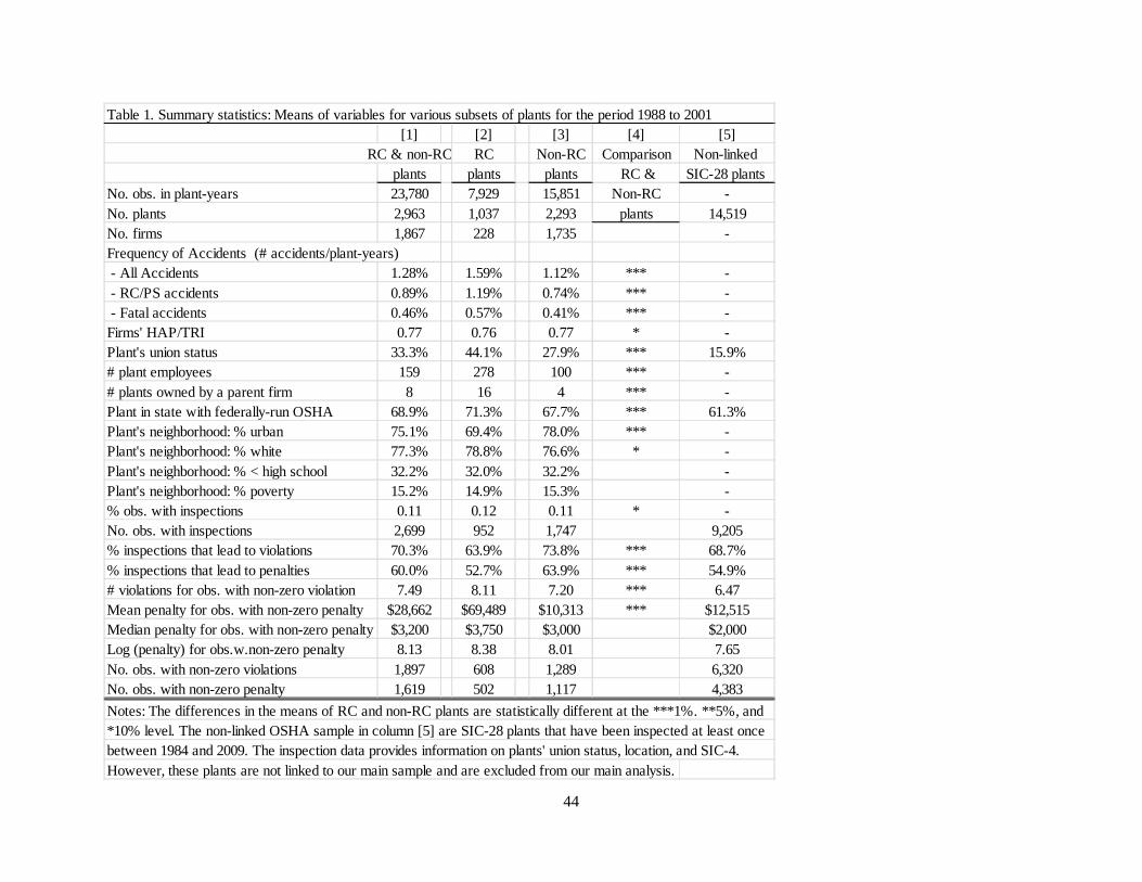
44

Table 1. Summary statistics: Means of variables for various subsets of plants for the period 1988 to 2001[1] [2] [3] [4] [5]

RC & non-RC RC Non-RC Comparison Non-linked plants plants plants RC & SIC-28 plants

No. obs. in plant-years 23,780 7,929 15,851 Non-RC -No. plants 2,963 1,037 2,293 plants 14,519No. firms 1,867 228 1,735 -Frequency of Accidents (# accidents/plant-years) - All Accidents 1.28% 1.59% 1.12% *** - - RC/PS accidents 0.89% 1.19% 0.74% *** - - Fatal accidents 0.46% 0.57% 0.41% *** -Firms' HAP/TRI 0.77 0.76 0.77 * -Plant's union status 33.3% 44.1% 27.9% *** 15.9%# plant employees 159 278 100 *** -# plants owned by a parent firm 8 16 4 *** -Plant in state with federally-run OSHA 68.9% 71.3% 67.7% *** 61.3%Plant's neighborhood: % urban 75.1% 69.4% 78.0% *** -Plant's neighborhood: % white 77.3% 78.8% 76.6% * -Plant's neighborhood: % < high school 32.2% 32.0% 32.2% -Plant's neighborhood: % poverty 15.2% 14.9% 15.3% -% obs. with inspections 0.11 0.12 0.11 * -No. obs. with inspections 2,699 952 1,747 9,205% inspections that lead to violations 70.3% 63.9% 73.8% *** 68.7%% inspections that lead to penalties 60.0% 52.7% 63.9% *** 54.9%# violations for obs. with non-zero violation 7.49 8.11 7.20 *** 6.47Mean penalty for obs. with non-zero penalty $28,662 $69,489 $10,313 *** $12,515Median penalty for obs. with non-zero penalty $3,200 $3,750 $3,000 $2,000Log (penalty) for obs.w.non-zero penalty 8.13 8.38 8.01 7.65No. obs. with non-zero violations 1,897 608 1,289 6,320No. obs. with non-zero penalty 1,619 502 1,117 4,383Notes: The differences in the means of RC and non-RC plants are statistically different at the ***1%. **5%, and*10% level. The non-linked OSHA sample in column [5] are SIC-28 plants that have been inspected at least once between 1984 and 2009. The inspection data provides information on plants' union status, location, and SIC-4. However, these plants are not linked to our main sample and are excluded from our main analysis.

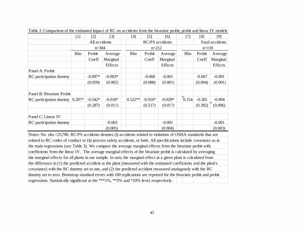
45

Table 2: Comparison of the estimated impact of RC on accidents from the bivariate probit, probit and linear IV models[1] [2] [3] [4] [5] [6] [7] [8] [9] All accidents RC/PS accidents Fatal accidents

n=304 n=212 n=110Rho Probit Average Rho Probit Average Rho Probit Average

Coeff Marginal Coeff Marginal Coeff Marginal Effects Effects Effects

Panel A: ProbitRC participation dummy -0.097* -0.003* -0.060 -0.001 -0.067 -0.001

(0.059)  (0.002) (0.088)  (0.001) (0.094)  (0.001)

Panel B: Bivariate ProbitRC participation dummy 0.287* -0.542* -0.018* 0.522** -0.916* -0.029* 0.154 -0.305 -0.004

(0.287)  (0.011) (0.517)  (0.017) (0.392) (0.006)

Panel C: Linear IVRC participation dummy -0.003 -0.001 -0.001 (0.005) (0.004) (0.003)Notes: No. obs.=23,780. RC/PS accidents denotes (i) accidents related to violations of OSHA standards that are related to RC codes of conduct or (ii) process safety accidents, or both. All specifications include covariates as in the main regressions (see Table 3). We compare the average marginal effects from the bivariate probit with coefficients from the linear IV. The average marginal effects of the bivariate probit is calculated by averagingthe marginal effects for all plants in our sample. In turn, the marginal effect at a given plant is calculated from the difference in (1) the predicted accident at the plant (measured with the estimated coefficients and the plant'scovariates) with the RC dummy set to one, and (2) the predicted accident measured analagously with the RCdummy set to zero. Bootstrap standard errors with 100 replications are reported for the bivariate probit and probitregressions. Statistically significant at the ***1%, **5% and *10% level, respectively.

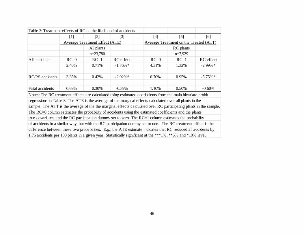
46

Table 3: Treatment effects of RC on the likelihood of accidents[1] [2] [3] [4] [5] [6]

Average Treatment Effect (ATE) Average Treatment on the Treated (ATT)All plants RC plantsn=23,780 n=7,929

All accidents RC=0 RC=1 RC effect RC=0 RC=1 RC effect2.46% 0.71% -1.76%* 4.31% 1.32% -2.99%*

RC/PS accidents 3.35% 0.42% -2.92%* 6.70% 0.95% -5.75%*

Fatal accidents 0.69% 0.30% -0.39% 1.10% 0.50% -0.60%Notes: The RC treatment effects are calculated using estimated coefficients from the main bivariate probitregressions in Table 3. The ATE is the average of the marginal effects calculated over all plants in the sample. The ATT is the average of the the marginal effects calculated over RC participating plants in the sample.The RC=0 column estimates the probability of accidents using the estimated coefficients and the plants' true covariates, and the RC participation dummy set to zero. The RC=1 column estimates the probabilityof accidents in a similar way, but with the RC participation dummy set to one. The RC treatment effect is the difference between these two probabilities. E.g., the ATE estimate indicates that RC reduced all accidents by 1.76 accidents per 100 plants in a given year. Statistically significant at the ***1%, **5% and *10% level.

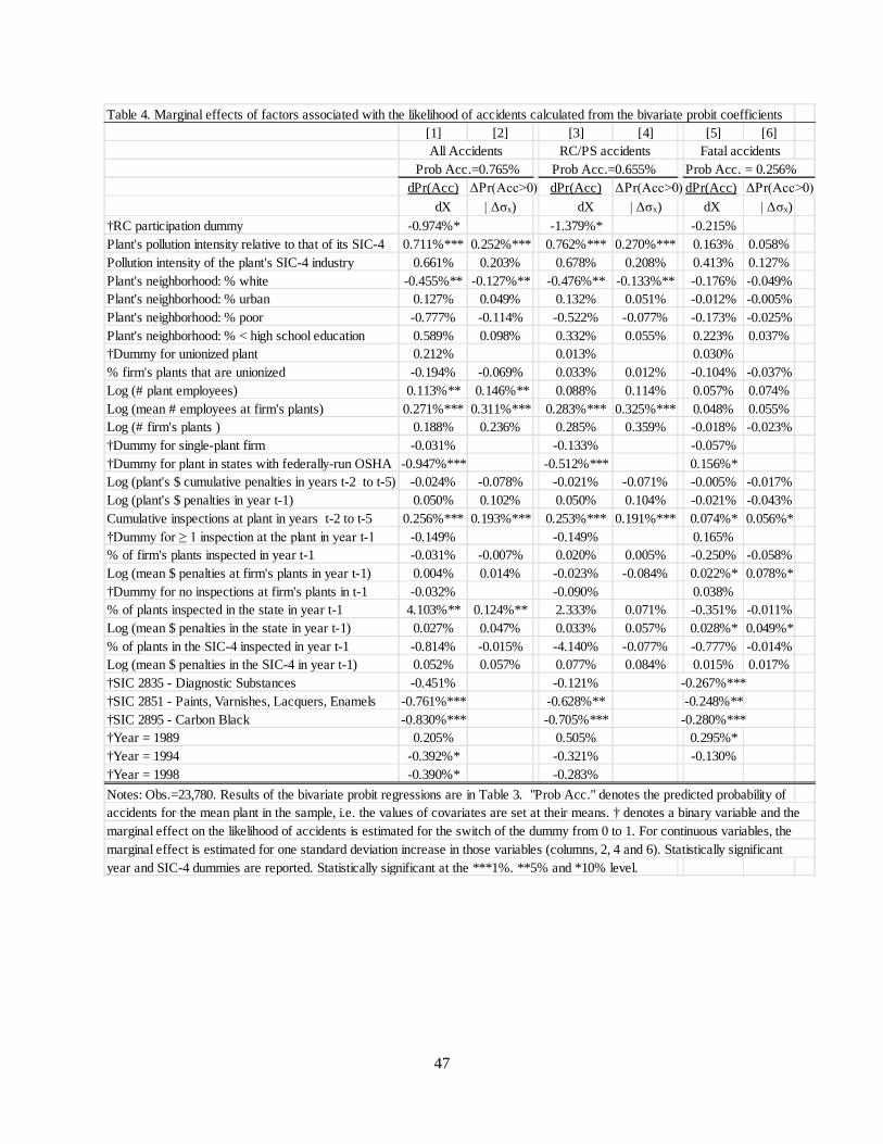
47

Table 4. Marginal effects of factors associated with the likelihood of accidents calculated from the bivariate probit coefficients[1] [2] [3] [4] [5] [6]

RC/PS accidents Fatal accidents Prob Acc.=0.765% Prob Acc.=0.655% Prob Acc. = 0.256%dPr(Acc) ΔPr(Acc>0)  dPr(Acc) ΔPr(Acc>0) dPr(Acc) ΔPr(Acc>0) 

dX     | Δσx) dX     | Δσx) dX     | Δσx)†RC participation dummy -0.974%* -1.379%* -0.215%Plant's pollution intensity relative to that of its SIC-4 0.711%*** 0.252%*** 0.762%*** 0.270%*** 0.163% 0.058%Pollution intensity of the plant's SIC-4 industry 0.661% 0.203% 0.678% 0.208% 0.413% 0.127%Plant's neighborhood: % white -0.455%** -0.127%** -0.476%** -0.133%** -0.176% -0.049%Plant's neighborhood: % urban 0.127% 0.049% 0.132% 0.051% -0.012% -0.005%Plant's neighborhood: % poor -0.777% -0.114% -0.522% -0.077% -0.173% -0.025%Plant's neighborhood: % < high school education 0.589% 0.098% 0.332% 0.055% 0.223% 0.037%†Dummy for unionized plant 0.212% 0.013% 0.030%% firm's plants that are unionized -0.194% -0.069% 0.033% 0.012% -0.104% -0.037%Log (# plant employees) 0.113%** 0.146%** 0.088% 0.114% 0.057% 0.074%Log (mean # employees at firm's plants) 0.271%*** 0.311%*** 0.283%*** 0.325%*** 0.048% 0.055%Log (# firm's plants ) 0.188% 0.236% 0.285% 0.359% -0.018% -0.023%†Dummy for single-plant firm -0.031% -0.133% -0.057%†Dummy for plant in states with federally-run OSHA -0.947%*** -0.512%*** 0.156%*Log (plant's $ cumulative penalties in years t-2 to t-5) -0.024% -0.078% -0.021% -0.071% -0.005% -0.017%Log (plant's $ penalties in year t-1) 0.050% 0.102% 0.050% 0.104% -0.021% -0.043%Cumulative inspections at plant in years t-2 to t-5 0.256%*** 0.193%*** 0.253%*** 0.191%*** 0.074%* 0.056%*†Dummy for ≥ 1 inspection at the plant in year t-1 -0.149% -0.149% 0.165%% of firm's plants inspected in year t-1 -0.031% -0.007% 0.020% 0.005% -0.250% -0.058%Log (mean $ penalties at firm's plants in year t-1) 0.004% 0.014% -0.023% -0.084% 0.022%* 0.078%*†Dummy for no inspections at firm's plants in t-1 -0.032% -0.090% 0.038%% of plants inspected in the state in year t-1 4.103%** 0.124%** 2.333% 0.071% -0.351% -0.011%Log (mean $ penalties in the state in year t-1) 0.027% 0.047% 0.033% 0.057% 0.028%* 0.049%*% of plants in the SIC-4 inspected in year t-1 -0.814% -0.015% -4.140% -0.077% -0.777% -0.014%Log (mean $ penalties in the SIC-4 in year t-1) 0.052% 0.057% 0.077% 0.084% 0.015% 0.017%†SIC 2835 - Diagnostic Substances -0.451% -0.121% -0.267%***†SIC 2851 - Paints, Varnishes, Lacquers, Enamels -0.761%*** -0.628%** -0.248%**†SIC 2895 - Carbon Black -0.830%*** -0.705%*** -0.280%***†Year = 1989 0.205% 0.505% 0.295%*†Year = 1994 -0.392%* -0.321% -0.130%†Year = 1998 -0.390%* -0.283%Notes: Obs.=23,780. Results of the bivariate probit regressions are in Table 3. "Prob Acc." denotes the predicted probability of accidents for the mean plant in the sample, i.e. the values of covariates are set at their means. † denotes a binary variable and the marginal effect on the likelihood of accidents is estimated for the switch of the dummy from 0 to 1. For continuous variables, the marginal effect is estimated for one standard deviation increase in those variables (columns, 2, 4 and 6). Statistically significant year and SIC-4 dummies are reported. Statistically significant at the ***1%. **5% and *10% level.

All Accidents

48

Online Appendix I: The role of top management in plant safety

Scholz and Gray (1990), based on field interviews and statistical research, report that

managerial attention to risk is an important component of a firm’s decision-making process on

safety issues. Drawing on Cyert and March’s (1963) behavioral theory of the firm, they note that:

(1) firms react to feedback rather than engage in long-run planning; (2) firms solve particular

problems, rather than general optimization, and; (3) firms learn, i.e., they “adapt goals and

attention rules as the environment changes” (Scholz and Gray, 1990). Similarly, accident

investigation reports note that the underlying cause of many accidents is the plants’ “poor safety

culture,” where safety culture is defined as: (1) the senior management’s commitment to safety

(Pidgeon and O’Leary 2000, Krause, 2004); and (2) the ability of the management and the

organization to learn from errors (Reason, 1997, cited in CSB-Texas City, 2007).

Senior managers play a key role in plant safety, first, they establish “objectives and

directives; they recommend safety management systems and site-level mechanisms such as

incident investigation, safety committees, safety action tracking systems, hazard analysis,

behavior observation and feedback” (NCBP, 2011). Second, in choosing the financing levels for

process safety systems, senior managers set the potential trade-off between production and

process safety (CCPS, 1992 cited in Baker Report, 2007). Moreover, “management not acting on

early warnings signs of problems” is noted as one root cause of chemical accidents investigated

by the EPA and OSHA (Belke, 1998). “An effective safety culture avoids incidents by being

informed,” i.e., by encouraging first, reporting, and second, learning (Reason, 1997, cited in

CSB-Texas City, 2007). In turn, the “reporting errors and near-misses requires an atmosphere of

trust, where personnel are encouraged to come forward and organizations promptly respond in a

meaningful way” (Reason, 1997, cited in CSB-Texas City, 2007). Further details on the role of

top management in plant safety, summarized from the accident investigation reports, are in

Finger and Gamper-Rabindran (2011).

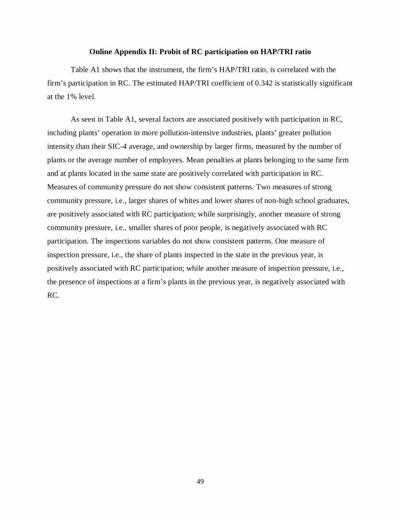
49

Online Appendix II: Probit of RC participation on HAP/TRI ratio

Table A1 shows that the instrument, the firm’s HAP/TRI ratio, is correlated with the

firm’s participation in RC. The estimated HAP/TRI coefficient of 0.342 is statistically significant

at the 1% level.

As seen in Table A1, several factors are associated positively with participation in RC,

including plants’ operation in more pollution-intensive industries, plants’ greater pollution

intensity than their SIC-4 average, and ownership by larger firms, measured by the number of

plants or the average number of employees. Mean penalties at plants belonging to the same firm

and at plants located in the same state are positively correlated with participation in RC.

Measures of community pressure do not show consistent patterns. Two measures of strong

community pressure, i.e., larger shares of whites and lower shares of non-high school graduates,

are positively associated with RC participation; while surprisingly, another measure of strong

community pressure, i.e., smaller shares of poor people, is negatively associated with RC

participation. The inspections variables do not show consistent patterns. One measure of

inspection pressure, i.e., the share of plants inspected in the state in the previous year, is

positively associated with RC participation; while another measure of inspection pressure, i.e.,

the presence of inspections at a firm’s plants in the previous year, is negatively associated with

RC.

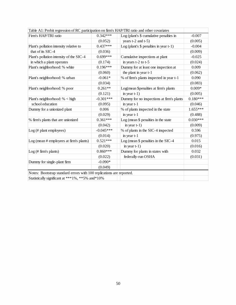
50

Table A1: Probit regression of RC participation on firm's HAP/TRI ratio and other covariatesFirm's HAP/TRI ratio 0.342*** Log (plant's $ cumulative penalties in -0.007

(0.052) years t-2 and t-5) (0.005)Plant's pollution intensity relative to 0.437*** Log (plant's $ penalties in year t-1) -0.004 that of its SIC-4 (0.036) (0.009)Plant's pollution intensity of the SIC-4 0.699*** Cumulative inspections at plant -0.025 in which a plant operates (0.174) in years t-2 to t-5 (0.024)Plant's neighborhood: % white 0.196*** Dummy for at least one inspection at 0.009

(0.060) the plant in year t-1 (0.062)Plant's neighborhood: % urban -0.061* % of firm's plants inspected in year t-1 0.090

(0.034) (0.083)Plant's neighborhood: % poor 0.261** Log(mean $penalties at firm's plants 0.009*

(0.121) in year t-1) (0.005)Plant's neighborhood: % < high -0.301*** Dummy for no inspections at firm's plants 0.180*** school education (0.095) in year t-1 (0.046)Dummy for a unionized plant 0.006 % of plants inspected in the state 1.655***

(0.029) in year t-1 (0.488)% firm's plants that are unionized 0.361*** Log (mean $ penalties in the state 0.030***

(0.042) in year t-1) (0.009)Log (# plant employees) -0.045*** % of plants in the SIC-4 inspected 0.596

(0.014) in year t-1 (0.975)Log (mean # employees at firm's plants) 0.521*** Log (mean $ penalties in the SIC-4 0.015

(0.020) in year t-1) (0.016)Log (# firm's plants) 0.860*** Dummy for plants in states with 0.032

(0.022) federally-run OSHA (0.031)Dummy for single-plant firm -0.090*

(0.049) Notes: Bootstrap standard errors with 100 replications are reported. Statistically significant at ***1%, **5% and*10%

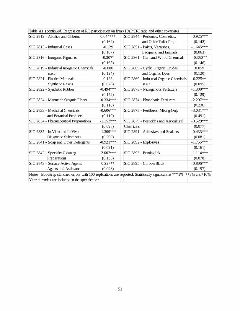
51

Table A1: (continued) Regression of RC participation on firm's HAP/TRI ratio and other covariatesSIC 2812 - Alkalies and Chlorine 0.644*** SIC 2844 - Perfumes, Cosmetics, -0.925***

(0.162) and Other Toilet Prep (0.142)SIC 2813 - Industrial Gases -0.129 SIC 2851 - Paints, Varnishes, -1.645***

(0.107) Lacquers, and Enamels (0.063)SIC 2816 - Inorganic Pigments -0.307* SIC 2861 - Gum and Wood Chemicals -0.350**

(0.165) (0.146)SIC 2819 - Industrial Inorganic Chemicals -0.080 SIC 2865 - Cyclic Organic Crudes 0.059 n.e.c. (0.124) and Organic Dyes (0.120)SIC 2821 - Plastics Materials 0.123 SIC 2869 - Industrial Organic Chemicals 0.225** Synthetic Resins (0.078) n.e.c. (0.095)SIC 2822 - Synthetic Rubber -0.494*** SIC 2873 - Nitrogenous Fertilizers -1.300***

(0.172) (0.129)SIC 2824 - Manmade Organic Fibers -0.334*** SIC 2874 - Phosphatic Fertilizers -2.297***

(0.118) (0.236)SIC 2833 - Medicinal Chemicals -0.606*** SIC 2875 - Fertilizers, Mixing Only -3.031*** and Botanical Products (0.119) (0.491)SIC 2834 - Pharmaceutical Preparations -1.152*** SIC 2879 - Pesticides and Agricultural -0.529***

(0.098) Chemicals (0.077)SIC 2835 - In Vitro and In Vivo -1.309*** SIC 2891 - Adhesives and Sealants -0.433*** Diagnostic Substances (0.200) (0.081)SIC 2841 - Soap and Other Detergents -0.921*** SIC 2892 - Explosives -1.755***

(0.091) (0.161)SIC 2842 - Specialty Cleaning -2.002*** SIC 2893 - Printing Ink -1.114*** Preparations (0.136) (0.078)SIC 2843 - Surface Active Agents 0.227** SIC 2895 - Carbon Black -0.806*** Agents and Assistants (0.098) (0.197)Notes: Bootstrap standard errors with 100 replications are reported. Statistically significant at ***1%, **5% and*10%Year dummies are included in the specification

52

Online Appendix III: Bivariate probit regressions of RC’s impact on accidents

Table A2: Bivariate probit regression on the impact of RC participation on plant-level accidents[1] [2] [3]

All accidents RC/PS accidents Fatal accidentsRC participation dummy -0.542* -0.916* -0.305

(0.287) (0.517) (0.392)Plant's pollution intensity relative to 0.337*** 0.415*** 0.206* that of its SIC-4 (0.066) (0.090) (0.122)Pollution intensity of the plant's 0.314 0.369 0.522 SIC-4 industry (0.315) (0.329) (0.413)Plant's neighborhood: % white -0.216** -0.259** -0.222

(0.105) (0.131) (0.193)Plant's neighborhood: % urban 0.060 0.072 -0.015

(0.067) (0.064) (0.082)Plant's neighborhood: % poor -0.369 -0.284 -0.218

(0.241) (0.211) (0.414)Plant's neighborhood: % <high 0.280 0.181 0.281 school edution (0.194) (0.166) (0.229)Dummy for unionized plant 0.096* 0.007 0.038

(0.056) (0.076) (0.088)% firm's plants that are unionized -0.092 0.018 -0.131

(0.083) (0.115) (0.118)Log (# plant employees) 0.054** 0.048 0.072

(0.025) (0.030) (0.055)Log (mean # employees at firm's 0.129*** 0.154** 0.061 plants) (0.041) (0.066) (0.066)Log (# firm's plants) 0.089 0.155 -0.023

(0.061) (0.102) (0.095)Dummy for single-plant firm -0.015 -0.074 -0.074

(0.079) (0.110) (0.112)Dummy for plants in states with -0.370*** -0.246*** 0.219** federally-run OSHA (0.055) (0.070) (0.095)Constant -3.645*** -4.039*** -4.088***

(0.498) (0.492) (0.749)Rho 0.287* 0.522** 0.154

(0.177) (0.250) (0.207)No obs. 23,780 23,780 23,780No accidents 304 212 110Notes: Bootstrap standard errors with 100 replications are reported. Statistically significant at the ***1%, **5%, and *10%

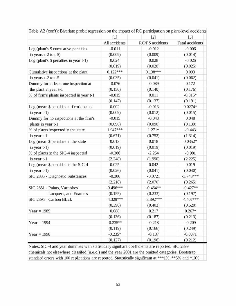
53

Table A2 (con't): Bivariate probit regression on the impact of RC participation on plant-level accidents[1] [2] [3]

All accidents RC/PS accidents Fatal accidentsLog (plant's $ cumulative penalties -0.011 -0.012 -0.006 in years t-2 to t-5) (0.009) (0.009) (0.014)Log (plant's $ penalties in year t-1) 0.024 0.028 -0.026

(0.019) (0.020) (0.025)Cumulative inspections at the plant 0.122*** 0.138*** 0.093 in years t-2 to t-5 (0.035) (0.041) (0.062)Dummy for at least one inspection at -0.076 -0.089 0.172 the plant in year t-1 (0.150) (0.140) (0.176)% of firm's plants inspected in year t-1 -0.015 0.011 -0.316*

(0.142) (0.137) (0.191)Log (mean $ penalties at firm's plants 0.002 -0.013 0.0274* in year t-1) (0.009) (0.012) (0.015)Dummy for no inspections at the firm's -0.015 -0.048 0.048 plants in year t-1 (0.096) (0.090) (0.139)% of plants inspected in the state 1.947*** 1.271* -0.443 in year t-1 (0.671) (0.752) (1.314)Log (mean $ penalties in the state 0.013 0.018 0.0352* in year t-1) (0.019) (0.019) (0.019)% of plants in the SIC-4 inspected -0.386 -2.254 -0.981 in year t-1 (2.248) (1.990) (2.225)Log (mean $ penalties in the SIC-4 0.025 0.042 0.019 in year t-1) (0.026) (0.041) (0.040)SIC 2835 - Diagnostic Substances -0.306 -0.0721 -3.743***

(2.218) (2.070) (0.265)SIC 2851 - Paints, Varnishes -0.496*** -0.464** -0.427** Lacquers, and Enamels (0.155) (0.233) (0.197)SIC 2895 - Carbon Black -4.329*** -3.892*** -4.407***

(0.396) (0.403) (0.520)Year = 1989 0.088 0.217 0.267*

(0.136) (0.187) (0.213)Year = 1994 -0.235** -0.218 -0.209

(0.119) (0.166) (0.249)Year = 1998 -0.235* -0.187 -0.0371

(0.127) (0.196) (0.212)Notes: SIC-4 and year dummies with statistically signifiant coefficients are reported. SIC 2899chemicals not elsewhere classifed (n.e.c.) and the year 2001 are the omitted categories. Bootstrapstandard errors with 100 replications are reported. Statistically significant at ***1%, **5% and *10%.

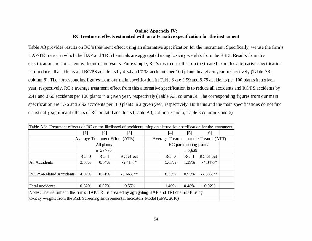
54

Online Appendix IV: RC treatment effects estimated with an alternative specification for the instrument

Table A3 provides results on RC’s treatment effect using an alternative specification for the instrument. Specifically, we use the firm’s

HAP/TRI ratio, in which the HAP and TRI chemicals are aggregated using toxicity weights from the RSEI. Results from this

specification are consistent with our main results. For example, RC’s treatment effect on the treated from this alternative specification

is to reduce all accidents and RC/PS accidents by 4.34 and 7.38 accidents per 100 plants in a given year, respectively (Table A3,

column 6). The corresponding figures from our main specification in Table 3 are 2.99 and 5.75 accidents per 100 plants in a given

year, respectively. RC’s average treatment effect from this alternative specification is to reduce all accidents and RC/PS accidents by

2.41 and 3.66 accidents per 100 plants in a given year, respectively (Table A3, column 3). The corresponding figures from our main

specification are 1.76 and 2.92 accidents per 100 plants in a given year, respectively. Both this and the main specifications do not find

statistically significant effects of RC on fatal accidents (Table A3, column 3 and 6; Table 3 column 3 and 6).

Table A3: Treatment effects of RC on the likelihood of accidents using an alternative specification for the instrument[1] [2] [3] [4] [5] [6]

Average Treatment Effect (ATE) Average Treatment on the Treated (ATT)All plants RC participating plantsn=23,780

RC=0 RC=1 RC effect RC=0 RC=1 RC effectAll Accidents 3.05% 0.64% -2.41%* 5.63% 1.29% -4.34%*

RC/PS-Related Accidents 4.07% 0.41% -3.66%** 8.33% 0.95% -7.38%**

Fatal accidents 0.82% 0.27% -0.55% 1.40% 0.48% -0.92%Notes: The instrument, the firm's HAP/TRI, is created by agregating HAP and TRI chemicals usingtoxicity weights from the Risk Screening Environmental Indicators Model (EPA, 2010)

n=7,929

55

We examine the relationship between the firm’s toxicity weighted HAP/TRI ratio and the firm’s participation in RC. In the probit

regression of RC participation on firm’s toxicity weighted HAP/TRI ratio and other covariates, the coefficient on firm’s HAP/TRI

ratio is 0.515 and statistically significant at the 5% level. The toxicity weighted HAP/TRI ratio has a mean of 0.78 for RC plants and a

mean of 0.79 for non-RC plants, respectively, and these means are statistically different at the 10% level.

56

Online Appendix V: Propensity Score Matching Method

Our preferred method is the bivariate probit, instrumenting for firms’ selection into RC

using firms’ HAP/TRI ratio. The strength of this approach is its ability to address firms’ selection

into RC based on unobserved factors. Firms are likely to have private information that jointly

affects their decision to join RC and the likelihood of an accident at their plants. We believe the

evidence is persuasive on the exclusion requirement. Firms’ HAP/TRI ratio affect their

contemporaneous decision to join RC, but are not directly related to accidents at their plants. We

note that this assumption cannot be empirically tested.

As a comparison to the bivariate probit, we apply the Propensity Score Matching (PSM)

method, which does not rely on the exclusion requirements for identification. Overall, the PSM

results support our main results from the bivariate probit, i.e., RC reduces the likelihood of all

accidents and PS/RC accidents, though the PSM estimates are about half the size of the estimates

from the bivariate probit. The PSM ATE estimate for all accidents indicates a reduction of 0.80

accidents per 100 plants in a given year, while the corresponding bivariate probit ATE estimate

indicates a reduction of 1.76 accidents per 100 plants in a given year. However, we note that the

PSM method suffers from an important drawback, i.e., it assumes that matching on the

observables can fully control for the differences between the RC and non-RC participants, and

thus, identify the effect of RC. In reality, it is likely that firms self-select into the RC program

based on unobserved factors.

Method

PSM has been applied to analyses of binary outcomes, e.g., estimating the effects of job

training on employment and medical surgeries on mortality (GAO, 1994; Aakvik, 2001;

Caliendo, Hujer, and Thomson, 2008). PSM estimates are based on comparing the likelihood of

accidents at RC participating plants to the likelihood at non-RC participating plants with similar

propensity scores. The ATT measures the difference in (a) the likelihood of accidents for RC

plants and (b) the corresponding likelihood for non-RC plants that are matched to the respective

RC plants. The ATE measures the difference in (c) the weighted average likelihood of accidents

at an RC plant and (d) the weighted average likelihood of accidents at a non-RC plant. In turn,

the value (c) is estimated from observed RC plants and RC plants that are matched to observed

57

non-RC plants. The value (d) is estimated from the observed non-RC plants and those matched to

observed RC plants.

The ATE and ATT are only identified in regions of common support, i.e., for similar

propensity scores, observations of both RC plants and non-RC plants are needed (Heckman,

LaLonde, and Smith, 1999). Based on our bivariate probit estimates, the likelihood of an

accident at the 25th percentile plant is 0.37 accidents per 100 plants in a given year, while the

likelihood at the 75th percentile is 1.94 accidents per 100 plants in a given year. To make a valid

comparison, RC plants at a specific range of propensity scores need to be compared with non-RC

plants that are similar in their range of propensity scores. In the case where there are sizable

numbers of non-RC plants to serve as matches, we would be able draw an inference on the

likelihood of accidents for the non-RC plants. In contrast, consider the extreme case in which

only a single non-RC plant is available to serve as the match. We would have the impossible task

of inferring the likelihood of accidents from the single matched plant, which would have had

either no accident or an accident.

Trimming the sample restricts our analysis to regions of common support (Smith and

Todd, 2005). We generate propensity scores using a probit model of RC participation on

covariates. We trim the sample by dropping observations at the top and bottom quintiles of the

propensity scores – the top quintiles are populated largely by RC plants, while the bottom

quintiles are populated largely by non-RC plants. Observations in the middle three quintiles have

estimated propensity scores between 0.0030 and 0.78. While trimming results in the loss of 40%

of our observations, it ensures that our analyses are restricted to regions with sufficient data to

enable appropriate matches and therefore, yield reasonable inferences.

We use nearest neighbor matching, in which a treatment case (RC plant) is compared

with the control case (non-RC plant) that is the closest match based on the absolute value of the

difference in their propensity scores. Matching is done with or without replacement; matching

with replacement allows a control case to be used as a match for more than one treated case.

Results

Our preferred specification, matching nearest neighbors (1-NN) with replacement on the

trimmed sample, is presented in Table A4, column 1. Overall, the PSM results support our main

results from the bivariate probit that RC reduced all accidents and PS/RC accidents. However,

the PSM estimates are about half the size of the IV estimates. Based on the ATE estimates, RC

58

reduces all accidents by 0.80 accidents per 100 plants in a given year and RC reduces RC/PS

accidents by 0.54 accidents per 100 plants in a given year. The ATT estimates for RC/PS

accidents are similar to the ATE estimates, i.e., RC leads to reduction of 0.70 RC/PS accidents

per 100 plants in a given year. The ATT estimates for all accidents are not statistically

significant. Effects on fatal accidents are not statistically significant for either the ATE or the

ATT estimates.

Next, we consider variations in the matching procedure. Our PSM results are robust to

the use of oversampling, i.e., using 5 closest matches (5-NN) (column 2). The ATE estimates are

similar for all accidents and PS/RC accidents, whether we match nearest neighbors or use

oversampling (column 1 and 2, respectively). The ATE estimates for fatal accidents are both

negative, but statistically significant only in the oversampling specification. For the ATT

estimates, the size of the coefficients for all accidents and PS/RC accidents are comparable in the

1-NN and 5-NN specifications, and their signs are both negative, but the coefficients are

significant in only one of the two specifications. The ATE estimates, unsurprisingly, are less

sensitive than the ATT estimates to variations in the matching procedure because the effects at

the highest and lowest percentiles of the propensity score even out.

Our preferred specification with the trimmed sample is matching with replacement. For

comparison, we show the nearest neighbor matching with no replacement in the trimmed sample

in column 3. The non-replacement procedure results in estimates that are smaller in magnitude

and the estimates are no longer significant. Only the ATT estimates of RC/PS accidents remains

statistically significant. The rarity of accidents in our sample is likely to make our analysis

sensitive to the replacement method. When matching is done without replacement, a control

case is used only once. This means that there are fewer available observations for subsequent

matching, leading to less precise matches. However, more unique controls are used as

counterfactuals, increasing the efficiency of the estimates. The median difference between

propensity scores with replacement in column 1 is 0.00018, while the median difference without

replacement in column 2 is 0.289.

Our preferred procedure is to trim the sample. For comparison, we present the results

from the nearest neighbor matching with replacement on a sample that is not trimmed. As seen in

column 4, the failure to trim leads to ATT estimates that are positive and statistically significant.

Examination of our sample indicates that matching a large number of observations to a relatively

59

small number of controls in the top and bottom quintiles of the propensity score are driving these

results.38

We consider one alternative to trimming as a strategy to improve the quality of matches.

Using the 1-NN matching, we specify a caliper and match without replacement. Specifying the

caliper, which requires the control case’s propensity score to be within a certain distance, helps

reduce cases of poor matches. Specifying no replacement avoids the situation in which the few

cases of poor matches in the top and bottom quintiles drive the results in the non-trimmed

sample. As seen in column 5, the specification with a caliper and no replacement in the non-

trimmed sample yields coefficients that are negative but not statistically significant for all

accidents and PS/RC accidents for both the ATE and ATT estimates. The coefficients for fatal

accidents are not statistically significant.

Conclusion

Overall, the PSM results support our main results from the bivariate probit, i.e., RC

reduced all accidents and PS/RC accidents. Both the bivariate probit (Table 3) and the PSM

models (Table A4, column 1) yield negative and statistically significant estimates. The PSM

estimates are about half the size of the estimates from the bivariate probit. It is not surprising that

the PSM model, which makes the conditional independence assumption, yields estimates that are

smaller in magnitude than the bivariate probit. The direction of bias when self-selection based on

unobservables is not addressed, as revealed in the comparison of the probit and bivariate probit

models (section 4.2), is to understate the effect of RC in reducing accidents.

38When we match with replacement in the non-trimmed sample, the 4,748 non-RC observations in the bottom quintile of propensity scores are matched to only 9 distinct RC observations that do not experience any accidents. In contrast, the 4,484 RC observations from the top quintile are matched to only 266 different non-RC observations all of which experience accidents. The effect at the bottom quintile makes the RC program look effective, while that at the top quintile makes the RC program look ineffective. Overall, the effect that RC fails to reduce accidents dominates the final estimates of ATT in the non-trimmed sample.

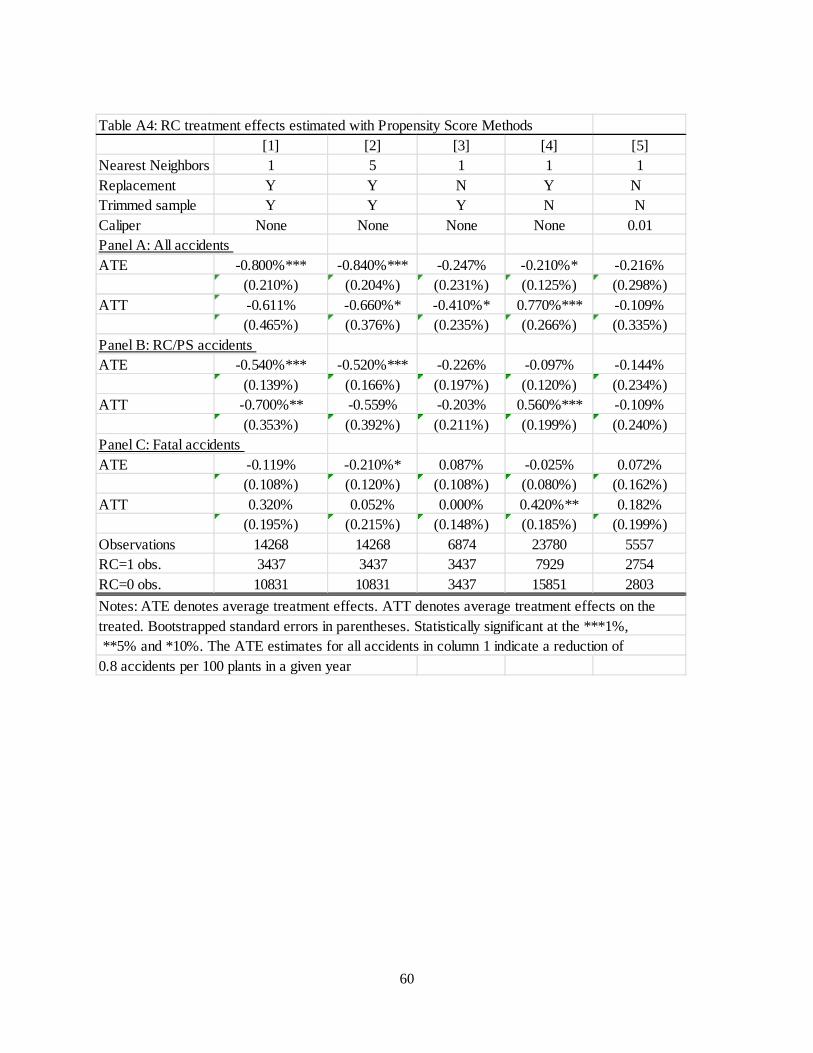
60

Table A4: RC treatment effects estimated with Propensity Score Methods[1] [2] [3] [4] [5]

Nearest Neighbors 1 5 1 1 1Replacement Y Y N Y N Trimmed sample Y Y Y N NCaliper None None None None 0.01Panel A: All accidents ATE -0.800%*** -0.840%*** -0.247% -0.210%* -0.216%

(0.210%) (0.204%) (0.231%) (0.125%) (0.298%)ATT -0.611% -0.660%* -0.410%* 0.770%*** -0.109%

(0.465%) (0.376%) (0.235%) (0.266%) (0.335%)Panel B: RC/PS accidents ATE -0.540%*** -0.520%*** -0.226% -0.097% -0.144%

(0.139%) (0.166%) (0.197%) (0.120%) (0.234%)ATT -0.700%** -0.559% -0.203% 0.560%*** -0.109%

(0.353%) (0.392%) (0.211%) (0.199%) (0.240%)Panel C: Fatal accidents ATE -0.119% -0.210%* 0.087% -0.025% 0.072%

(0.108%) (0.120%) (0.108%) (0.080%) (0.162%)ATT 0.320% 0.052% 0.000% 0.420%** 0.182%

(0.195%) (0.215%) (0.148%) (0.185%) (0.199%)Observations 14268 14268 6874 23780 5557RC=1 obs. 3437 3437 3437 7929 2754RC=0 obs. 10831 10831 3437 15851 2803Notes: ATE denotes average treatment effects. ATT denotes average treatment effects on thetreated. Bootstrapped standard errors in parentheses. Statistically significant at the ***1%, **5% and *10%. The ATE estimates for all accidents in column 1 indicate a reduction of 0.8 accidents per 100 plants in a given year