Embed Size (px)
Citation preview
Introduction Model Results Conclusion
Does Human Capital Risk Explain The ValuePremium Puzzle?
Serginio Sylvain
Department of EconomicsUniversity of Chicago
Current Draft: March, 2014First Draft: January, 2013
1 / 25

Introduction Model Results Conclusion
OutlineIntroduction
MotivationLiterature
Model
PrimitivesPlanner’s ProblemEquilibriumAsset Pricing Implications
Results
Fama and French (1996, 1997)Empirical Evidence and Implications of the ModelCyclicity and Long Run RiskThe CAPM
Conclusion2 / 25
Introduction Model Results Conclusion
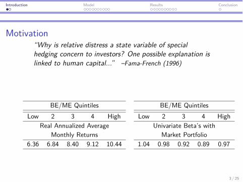
Motivation“Why is relative distress a state variable of specialhedging concern to investors? One possible explanation islinked to human capital...” –Fama-French (1996)
BE/ME QuintilesLow 2 3 4 High
Real Annualized AverageMonthly Returns
6.36 6.84 8.40 9.12 10.44
BE/ME QuintilesLow 2 3 4 High
Univariate Beta’s withMarket Portfolio
1.04 0.98 0.92 0.89 0.97
3 / 25

Introduction Model Results Conclusion
LiteratureI The Value Premium: Fama and French (1996; 1997; 1998),
Rouwenhorst (1999), Liew and Vassalou (2000), ...
I Empirical literature on Value Premium, human capital and laborincome: Jaganathan and Wang (1996), Jagannathan et al. (1998),Hansson (2004), Veronesi and Santos (2005), ...
I Some more theoretical approaches: Veronesi and Santos (2005),Zhang (2005), Bansal, Dittmar and Lundblad (2005), Hansen,Heaton and Li (2008), Garleanu, Kogan, and Panageas (2012), ...
I I complement the above research by producing a generalequilibrium model with endogenous growth where the ValuePremium arises endogenously from risk to human capital.
I I draw from the recent literature on asset pricing in aproduction economy: Kogan (2001, 2003), Eberly and Wang(2009, 2011), ... 4 / 25
Introduction Model Results Conclusion
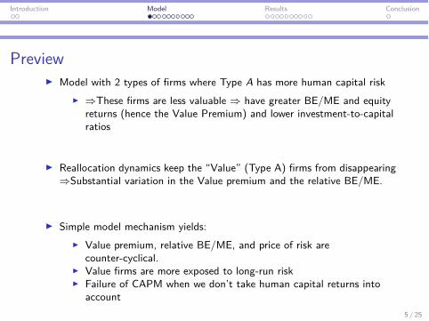
PreviewI Model with 2 types of firms where Type A has more human capital risk
I ∆These firms are less valuable ∆ have greater BE/ME and equityreturns (hence the Value Premium) and lower investment-to-capitalratios
I Reallocation dynamics keep the “Value” (Type A) firms from disappearing∆Substantial variation in the Value premium and the relative BE/ME.
I Simple model mechanism yields:I Value premium, relative BE/ME, and price of risk are
counter-cyclical.I Value firms are more exposed to long-run riskI Failure of CAPM when we don’t take human capital returns into
account5 / 25

Introduction Model Results Conclusion
I Evidence: Value firms are more exposed to human capital risk
I Possible Explanations:I Aggr. human capital productivity covary more positively with
outcomes of Value firms: “negative shock to a distressed firm [...]implies a negative shock to the value of specialized human capital...Thus, workers avoid the stocks of [all] distressed firms.”–F&F(’96)
I Value firms have relatively more firm-specific human capital andhence are more burdened by their wage bill
6 / 25
Introduction Model Results Conclusion
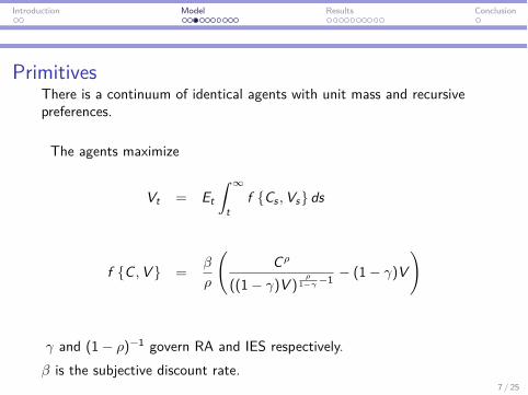
PrimitivesThere is a continuum of identical agents with unit mass and recursivepreferences.
The agents maximize
Vt = Et
⁄ Œ
tf {Cs , Vs} ds
f {C , V } =—
fl
ACfl
((1 ≠ “)V )fl
1≠“ ≠1 ≠ (1 ≠ “)VB
“ and (1 ≠ fl)≠1 govern RA and IES respectively.— is the subjective discount rate.
7 / 25

Introduction Model Results Conclusion
At date zero, each agent is endowed with human capital H0.
There are 2 types of firms; each with a continuum (with unit mass) ofidentical firms endowed with physical capital K i
0 = K0 for i œ {A, B}.
Type A firms use physical capital (KA) and human capital (H) as inputsto production.
Firms of Type B use physical capital (KB).
8 / 25
Introduction Model Results Conclusion
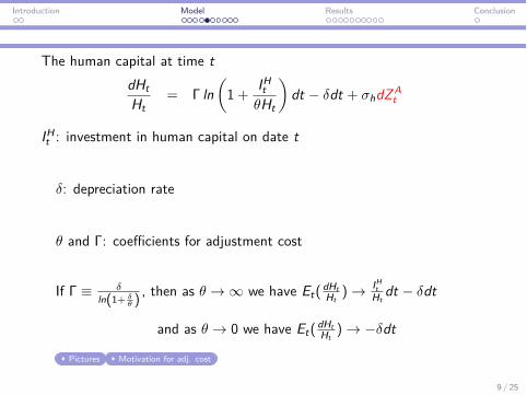
The human capital at time tdHtHt
= � ln3
1 +IHt
◊Ht
4dt ≠ ”dt + ‡hdZA
t
IHt : investment in human capital on date t
”: depreciation rate
◊ and �: coe�cients for adjustment cost
If � © ”ln(1+ ”
◊ ), then as ◊ æ Œ we have Et(
dHtHt
) æ IHt
Htdt ≠ ”dt
and as ◊ æ 0 we have Et(dHtHt
) æ ≠”dt
Pictures Motivation for adj. cost
9 / 25
Introduction Model Results Conclusion
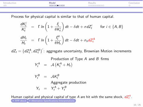
Process for physical capital is similar to that of human capital.
dK it
K it
= � ln3
1 +I it
◊K it
4dt ≠ ”dt + ‡dZ i
t for i œ {A, B}
dHtHt
= � ln3
1 +IHt
◊Ht
4dt ≠ ”dt + ‡hdZA
t
dZt = {dZAt , dZB
t }Õ : aggregate uncertainty, Brownian Motion increments
Production of Type A and B firmsY A
t = A!KA
t + Ht"
Y Bt = AKB
tAggregate production
Yt = Y At + Y B
t
Human capital and physical capital of type A are hit with the same shock, dZ At .
TFP shock Alternative Specifications/Interpretations10 / 25
Introduction Model Results Conclusion
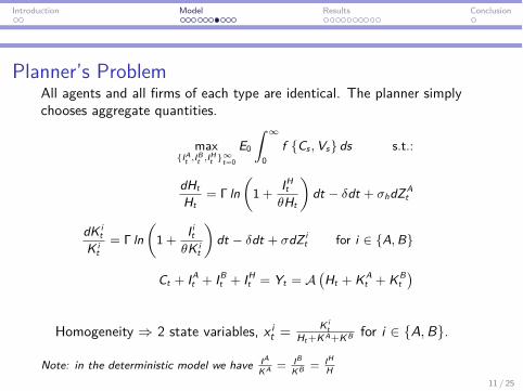
Planner’s ProblemAll agents and all firms of each type are identical. The planner simplychooses aggregate quantities.
max{IA
t ,IBt ,IH
t }Œt=0
E0
⁄ Œ
0f {Cs , Vs} ds s.t.:
dHtHt
= � ln3
1 +IHt
◊Ht
4dt ≠ ”dt + ‡hdZ A
t
dK it
K it
= � ln3
1 +I it
◊K it
4dt ≠ ”dt + ‡dZ i
t for i œ {A, B}
Ct + IAt + IB
t + IHt = Yt = A
!Ht + KA
t + KBt
"
Homogeneity ∆ 2 state variables, x it =
Kit
Ht+KA+KB for i œ {A, B}.
Note: in the deterministic model we have IA
KA = IB
KB = IHH
11 / 25

Introduction Model Results Conclusion
EquilibriumAn equilibrium consists of a set of adapted processes {Ct , IA
t , IBt , IH
t }’tsuch that
1. {IAt , IB
t , IHt } solve the Hamiltonian-Jacobi-Bellman equation
2. resource constraint is satisfied: Ct + IAt + IB
t + IHt = Yt where
Yt = A!Ht + KA
t + KBt
"
3. the LOM for aggregate human and physical capital are satisfied
dHtHt
= � ln3
1 +IHt
◊Ht
4dt ≠ ”dt + ‡hdZA
t
dKit
K it
= � ln3
1 +I it
◊Kit
4dt ≠ ”dt + ‡dZi
t for i œ {A, B}
12 / 25

Introduction Model Results Conclusion
Asset PricingThere are 2 risky securities: risky claims on sum of profits of 2 firm types.
Let ÿH = IH
H , and ÿi = I i
K i
qit : the value of physical of type i (Tobin Q)
qi =1�
!ÿi + ◊
"
pt : the value of human capital (Tobin Q)
p =1�
!ÿH + ◊
"
Stochastic Discount Factor, ⇤t , follows Decentralized Problem formulas
d⇤t⇤t
= ≠rtdt ≠ ‡⇤,t · dZt
13 / 25
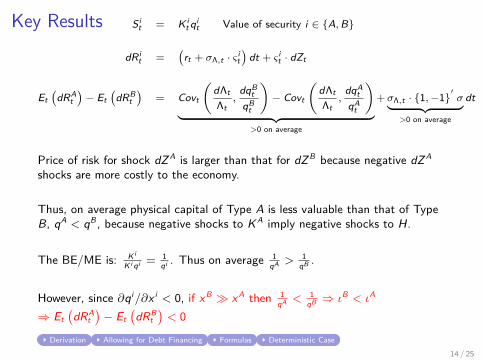
Key Results Sit = Ki
t qit Value of security i œ {A, B}
dRit =
!rt + ‡⇤,t · Î i
t"
dt + Î it · dZt
Et!
dRAt"
≠ Et!
dRBt
"= Covt
3d⇤t⇤t
,dqB
tqB
t
4≠ Covt
3d⇤t⇤t
,dqA
tqA
t
4
¸ ˚˙ ˝>0 on average
+‡⇤,t · {1, ≠1}Õ
‡¸ ˚˙ ˝>0 on average
dt
Price of risk for shock dZ A is larger than that for dZ B because negative dZ A
shocks are more costly to the economy.
Thus, on average physical capital of Type A is less valuable than that of TypeB, qA < qB , because negative shocks to KA imply negative shocks to H.
The BE/ME is: Ki
Ki qi = 1qi . Thus on average 1
qA > 1qB .
However, since ˆqi /ˆx i < 0, if xB ∫ xA then 1qA < 1
qB ∆ ÿB < ÿA
∆ Et!dRA
t"
≠ Et!dRB
t"
< 0
Derivation Allowing for Debt Financing Formulas Deterministic Case14 / 25
Introduction Model Results Conclusion
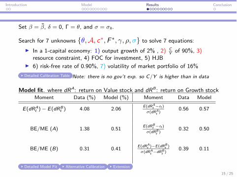
Set — = —, ” = 0, � = ◊, and ‡ = ‡h.
Search for 7 unknowns {◊, A, cú, F ú, “, fl, ‡} to solve 7 equations:I In a 1-capital economy: 1) output growth of 2% , 2) C
Y of 90%, 3)resource constraint, 4) FOC for investment, 5) HJB
I 6) risk-free rate of 0.90%, 7) volatility of market portfolio of 16%Detailed Calibration Table Note: there is no gov’t exp. so C/Y is higher than in data
Model fit. where dRA: return on Value stock and dRB : return on Growth stockMoment Data (%) Model (%) Moment Data Model
E(dRAt ) ≠ E(dRB
t ) 4.08 2.06 E(dRAt ≠rt )
‡(dRAt )
0.56 0.57
BE/ME (A) 1.38 0.51 E(dRBt ≠rt )
‡(dRBt )
0.32 0.50
BE/ME (B) 0.31 0.41 E(dRAt )≠E(dRB
t )
‡(dRAt ≠dRB
t )0.39 0.11
Detailed Model Fit Alternative Calibration Extension15 / 25
Introduction Model Results Conclusion
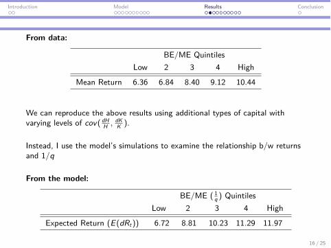
From data:
BE/ME QuintilesLow 2 3 4 High
Mean Return 6.36 6.84 8.40 9.12 10.44
We can reproduce the above results using additional types of capital withvarying levels of cov( dH
H , dKK ).
Instead, I use the model’s simulations to examine the relationship b/w returnsand 1/q
From the model:
BE/ME ( 1q ) Quintiles
Low 2 3 4 High
Expected Return (E(dRt)) 6.72 8.81 10.23 11.29 11.97
16 / 25
Introduction Model Results Conclusion
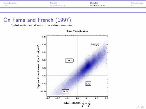
On Fama and French (1997)Substantial variation in the value premium...
17 / 25
Introduction Model Results Conclusion
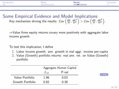
Some Empirical Evidence and Model ImplicationsKey mechanism driving the results: Cov
1dHH , dKA
KA
2> Cov
1dHH , dKB
KB
2.
∆Value firms equity returns covary more positively with aggregate laborincome growth.
To test this implication, I define1. Labor income growth: ann. growth in real aggr. income per-capita2. Value (Growth) portfolio returns: real ann. ret. on Value (Growth)
portfolio
Aggregate Human Capital—i,h P-val
Value Portfolio 1.96 0.03Growth Portfolio 0.82 0.38
more
18 / 25
Introduction Model Results Conclusion
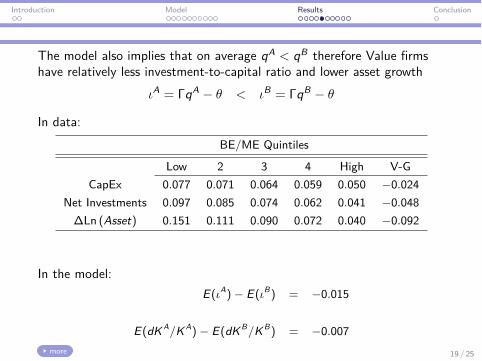
The model also implies that on average qA < qB therefore Value firmshave relatively less investment-to-capital ratio and lower asset growth
ÿA = �qA ≠ ◊ < ÿB = �qB ≠ ◊
In data:BE/ME Quintiles
Low 2 3 4 High V-GCapEx 0.077 0.071 0.064 0.059 0.050 ≠0.024
Net Investments 0.097 0.085 0.074 0.062 0.041 ≠0.048�Ln (Asset) 0.151 0.111 0.090 0.072 0.040 ≠0.092
In the model:E(ÿA) ≠ E(ÿB) = ≠0.015
E(dKA/KA) ≠ E(dKB/KB) = ≠0.007more 19 / 25
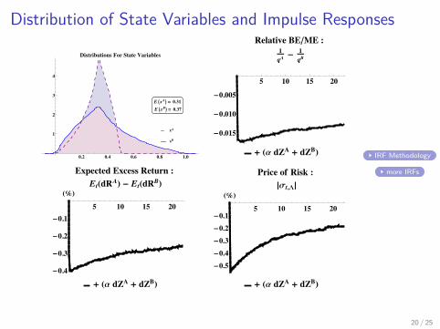
Distribution of State Variables and Impulse Responses
xA
xB
0.2 0.4 0.6 0.8 1.0
1
2
3
4
Distributions For State Variables
E !xA" ! 0.31
E !xB" ! 0.37
5 10 15 20
-0.015
-0.010
-0.005
Relative BEêME :1qA- 1qB
+ Ha dZA + dZBL
5 10 15 20
-0.4
-0.3
-0.2
-0.1
H%LExpected Excess Return :
EtHdRAL - EtHdRBL
+ Ha dZA + dZBL
5 10 15 20
!0.5
!0.4
!0.3
!0.2
!0.1
!""
Price of Risk :
#Σt,$#
% !Α dZA % dZB"
IRF Methodology
more IRFs
20 / 25
Introduction Model Results Conclusion
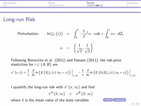
Long-run Risk
Perturbation: ln (’t {‘}) =
⁄ t
0≠1
2‘2– · –ds +⁄ t
0‘– · dZs
– =
;1Ô2
,1Ô2
<Õ
Following Borovicka et al. (2011) and Hansen (2011), the risk-priceelasticities for i œ {A, B} are
fii {x , t} =1t
dd‘
ln)
E!
Sit’t {‘} |x0 = x
"* ---‘=0
≠1t
dd‘
ln)
E!⇤tSi
t’t {‘} |x0 = x"* ---
‘=0
I quantify the long-run risk with fii {x , Œ} and findfiA {x , Œ} > fiB {x , Œ}
where x is the mean value of the state variables Plot (details)21 / 25

Introduction Model Results Conclusion
Conditional CAPMdRm
t and dRwt : returns on the market and total wealth portfolios.
dRm = dRAÊ + dRB(1 ≠ Ê) = µmt dt + Îm
t · dZt
dRw =
3dRH(1 ≠ ÊA ≠ ÊB) + dRAÊA
+dRBÊB
4= µw
t dt + Îwt · dZt
Consider the regression
Et!dRA
t"
≠ Et!dRB
t"
= –0¸˚˙˝Pricing Error
+ –1¸˚˙˝Slope
◊ Îwt .Îw
t!—A,w
t ≠ —B,wt
"dt
— i,wt =
covt(dR it , dRw
t )Îw
t .Îwt
for i œ {A, B}
With Log-Utitlity, the price of risk is ‡⇤,t = ‡c,t = Îwt ; thus the Conditional
CAPM holds: –0 = 0 and –1 = 1.
I will run the above regression with dRm and dRw and compare the pricing errors22 / 25

Introduction Model Results Conclusion
Conditional CAPM Regressions(1): Et
!dRA
t"
≠ Et!dRB
t"= –0¸˚˙˝
Pricing Error
+ –1¸˚˙˝Slope
◊ Îwt .Îw
t
1—A,w
t ≠ —B,wt
2dt
(2): Et!dRA
t"
≠ Et!dRB
t"= –0¸˚˙˝
Pricing Error
+ –1¸˚˙˝Slope
◊ Îmt .Îm
t
1—A,m
t ≠ —B,mt
2dt
“ = (1 ≠ fl) = 1 (log-utility) “ > (1 ≠ fl) ”= 1
–0 (%)t-stat
–1t-stat
R2
t-stat
(1) (2) Di�.0.00 1.1 ≠1.10.38 290. ≠290.
1. 0.97 0.041.3 ◊ 1016 290. 1.3 ◊ 1016
1. 1. 0.007000. 330. 1.5
(1) (2) Di�.≠0.06 1.9 ≠2.≠2.9 100. ≠110.
3.4 0.09 3.3370. 120. 260.
1. 0.97 0.03410. 33. 0.95
More23 / 25
Introduction Model Results Conclusion
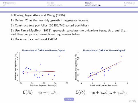
Following Jaganathan and Wang (1996):1) Define Rh
t as the monthly growth in aggregate income.2) Construct test portfolios (20 BE/ME sorted portfolios).3) Use Fama-MacBeth (1973) approach; calculate the univariate betas, —i,m and —i,h,and then compare cross-sectional regressions below4) Do same for conditional CAPM
.4.6
.81
1.2
1.4
Re
aliz
ed
Ave
rag
e R
etu
rn (
%)
.71 .72 .73 .74 .75Predicted Expected Return (%)
Unconditional CAPM w/o Human Capital
.4.6
.81
1.2
1.4
Re
aliz
ed
Ave
rag
e R
etu
rn (
%)
.4 .6 .8 1 1.2Predicted Expected Return (%)
Unconditional CAPM w/ Human Capital
E (Ri) = “0 + “m—i ,m E (Ri) = “0 + “m—i ,m + “h—i ,h
More24 / 25
Introduction Model Results Conclusion
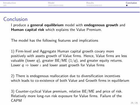
ConclusionI produce a general equilibrium model with endogenous growth andHuman capital risk which explains the Value Premium.
The model has the following features and implications
1) Firm-level and Aggregate Human capital growth covary morepositively with assets growth of Value firms. Hence, Value firms are lessvaluable (lower q), greater BE/ME (1/q), and greater equity returns.Lower q ∆ lower ÿ and lower asset growth for Value firms
2) There is endogenous reallocation due to diversification incentiveswhich leads to co-existence of both Value and Growth firms in equilibrium
3) Counter-cyclical Value premium, relative BE/ME and price of risk.Relatively more long-run risk exposure for Value firms. Failure of theCAPM
25 / 25
Additional Figures and Tables
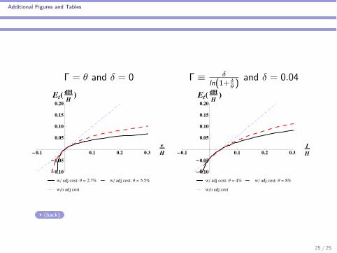
� = ◊ and ” = 0 � © ”ln(1+ ”
◊ )and ” = 0.04
!0.1 0.1 0.2 0.3
Ε
H
!0.10
!0.05
0.05
0.10
0.15
0.20
Et!dH
H"
w! adj cost: Θ " 2.7# w! adj cost: Θ " 5.5#
w!o adj cost
!0.1 0.1 0.2 0.3
I
H
!0.10
!0.05
0.05
0.10
0.15
0.20
Et!dH
H"
w! adj cost: Θ " 4# w! adj cost: Θ " 8#
w!o adj cost
(back)
25 / 25
Additional Figures and Tables
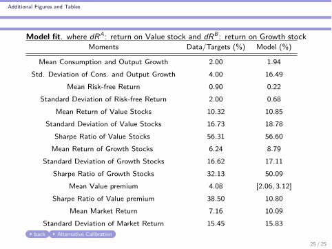
Model fit. where dRA: return on Value stock and dRB : return on Growth stockMoments Data/Targets (%) Model (%)
Mean Consumption and Output Growth 2.00 1.94Std. Deviation of Cons. and Output Growth 4.00 16.49
Mean Risk-free Return 0.90 0.22Standard Deviation of Risk-free Return 2.00 0.68
Mean Return of Value Stocks 10.32 10.85Standard Deviation of Value Stocks 16.73 18.78
Sharpe Ratio of Value Stocks 56.31 56.60Mean Return of Growth Stocks 6.24 8.79
Standard Deviation of Growth Stocks 16.62 17.11Sharpe Ratio of Growth Stocks 32.13 50.09
Mean Value premium 4.08 [2.06, 3.12]Sharpe Ratio of Value premium 38.50 10.80
Mean Market Return 7.16 10.09Standard Deviation of Market Return 15.45 15.83
back Alternative Calibration
25 / 25
Additional Figures and Tables
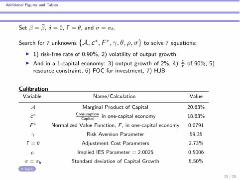
Set — = —, ” = 0, � = ◊, and ‡ = ‡h.
Search for 7 unknowns {A, cú, F ú, “, ◊, fl, ‡} to solve 7 equations:I 1) risk-free rate of 0.90%, 2) volatility of output growthI And in a 1-capital economy: 3) output growth of 2%, 4) C
Y of 90%, 5)resource constraint, 6) FOC for investment, 7) HJB
CalibrationVariable Name/Calculation Value
A Marginal Product of Capital 20.63%cú Consumption
Capital in one-capital economy 18.63%F ú Normalized Value Function, F , in one-capital economy 0.0791“ Risk Aversion Parameter 59.35
� = ◊ Adjustment Cost Parameters 2.73%fl Implied IES Parameter = 2.0025 0.5006
‡ = ‡h Standard deviation of Capital Growth 5.50%back
25 / 25

Additional Figures and Tables
Model fit. where dRA: return on Value stock and dRB : return on Growth stockMoments Data/Targets (%) Model (%)
Mean Consumption and Output Growth 2.00 2.02Std. Deviation of Cons. and Output Growth 4.00 4.08
Mean Risk-free Return 0.90 0.90Standard Deviation of Risk-free Return 2.00 0.14
Mean Return of Value Stocks 10.32 10.97Standard Deviation of Value Stocks 16.73 4.66
Sharpe Ratio of Value Stocks 56.31 216Mean Return of Growth Stocks 6.24 9.34
Standard Deviation of Growth Stocks 16.62 4.15Sharpe Ratio of Growth Stocks 32.13 204
Mean Value premium 4.08 [1.64, 1.65]Sharpe Ratio of Value premium 38.50 41.42
Mean Market Return 7.16 10.05Standard Deviation of Market Return 15.45 3.92
back
25 / 25
Additional Figures and Tables
25 / 25

Additional Figures and Tables
25 / 25
Additional Figures and Tables
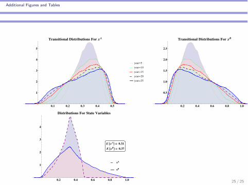
0.1 0.2 0.3 0.4 0.5
1
2
3
4
5
Transitional Distributions For xA
year!5
year!10
year!15
year!20
year!25
0.2 0.4 0.6 0.8 1.0
0.5
1.0
1.5
2.0
2.5
Transitional Distributions For xB
year!5
year!10
year!15
year!20
year!25
xA
xB
0.2 0.4 0.6 0.8 1.0
1
2
3
4
Distributions For State Variables
E !xA" ! 0.31
E !xB" ! 0.37
25 / 25
Additional Figures and Tables
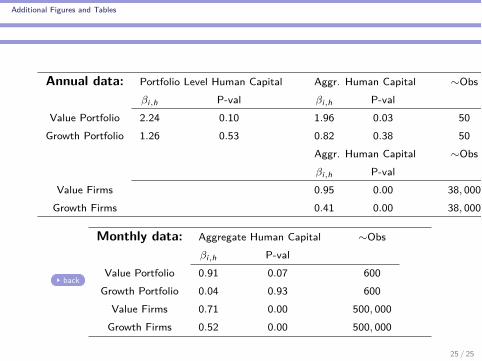
Annual data: Portfolio Level Human Capital Aggr. Human Capital ≥Obs—i,h P-val —i,h P-val
Value Portfolio 2.24 0.10 1.96 0.03 50Growth Portfolio 1.26 0.53 0.82 0.38 50
Aggr. Human Capital ≥Obs—i,h P-val
Value Firms 0.95 0.00 38, 000Growth Firms 0.41 0.00 38, 000
back
Monthly data: Aggregate Human Capital ≥Obs—i,h P-val
Value Portfolio 0.91 0.07 600Growth Portfolio 0.04 0.93 600
Value Firms 0.71 0.00 500, 000Growth Firms 0.52 0.00 500, 000
25 / 25
Additional Figures and Tables
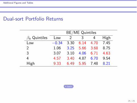
Dual-sort Portfolio Returns
BE/ME Quintiles—h Quintiles Low 2 3 4 HighLow ≠0.34 3.30 6.14 4.70 7.452 1.06 3.25 5.66 3.68 8.753 3.07 3.10 4.06 6.71 4.634 4.57 3.40 4.87 6.70 9.54High 9.33 6.49 5.95 7.48 8.21
back
25 / 25
Additional Figures and Tables
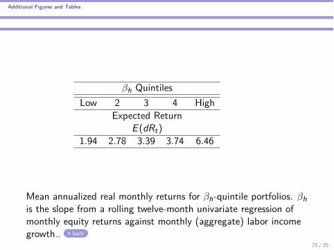
—h QuintilesLow 2 3 4 High
Expected ReturnE (dRt)
1.94 2.78 3.39 3.74 6.46
Mean annualized real monthly returns for —h-quintile portfolios. —his the slope from a rolling twelve-month univariate regression ofmonthly equity returns against monthly (aggregate) labor incomegrowth.. back
25 / 25
Additional Figures and Tables
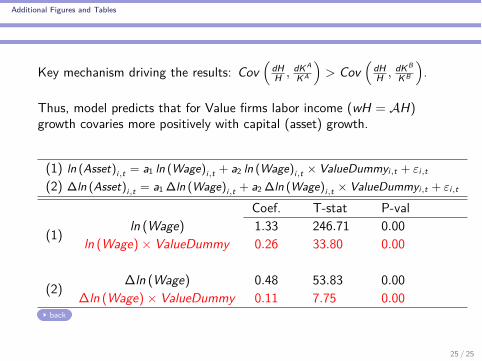
Key mechanism driving the results: Cov1
dHH , dKA
KA
2> Cov
1dHH , dKB
KB
2.
Thus, model predicts that for Value firms labor income (wH = AH)growth covaries more positively with capital (asset) growth.
(1) ln (Asset)i,t = a1 ln (Wage)i,t + a2 ln (Wage)i,t ◊ ValueDummyi,t + Ái,t
(2) �ln (Asset)i,t = a1 �ln (Wage)i,t + a2 �ln (Wage)i,t ◊ ValueDummyi,t + Ái,t
Coef. T-stat P-val
(1) ln (Wage) 1.33 246.71 0.00ln (Wage) ◊ ValueDummy 0.26 33.80 0.00
(2) �ln (Wage) 0.48 53.83 0.00�ln (Wage) ◊ ValueDummy 0.11 7.75 0.00
back
25 / 25

Additional Figures and Tables
Below I control for the number (or growth rate) of employees
(1) ln (Asset)i,t = a1 ln (Wage)i,t + a2 ln (Wage)i,t ◊ ValueDummyi,t
+a3 ln (Emp)i,t + Ái,t
(2) �ln (Asset)i,t = a1 �ln (Wage)i,t + a2 �ln (Wage)i,t ◊ ValueDummyi,t
+a3 �ln (Emp)i,t + Ái,t
Coef. T-stat P-value
(1)ln (Wage) 1.68 391.53 0.00
ln (Wage) ◊ ValueDummy 0.11 21.69 0.00ln (Emp) ≠0.92 ≠134.67 0.00
(2)�ln (Wage) 0.30 53.83 0.00
�ln (Wage) ◊ ValueDummy 0.07 7.75 0.00�ln (Emp) 0.47 50.34 0.00
back
25 / 25
Additional Figures and Tables
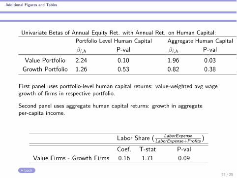
Univariate Betas of Annual Equity Ret. with Annual Ret. on Human Capital:Portfolio Level Human Capital Aggregate Human Capital—i,h P-val —i,h P-val
Value Portfolio 2.24 0.10 1.96 0.03Growth Portfolio 1.26 0.53 0.82 0.38
First panel uses portfolio-level human capital returns: value-weighted avg wagegrowth of firms in respective portfolio.
Second panel uses aggregate human capital returns: growth in aggregateper-capita income.
Labor Share ( LaborExpenseLaborExpense+Profits )
Coef. T-stat P-valValue Firms - Growth Firms 0.16 1.71 0.09
back25 / 25
Additional Figures and Tables
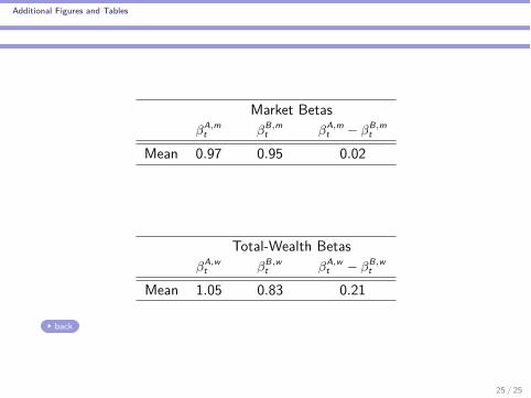
Market Betas—A,m
t —B,mt —A,m
t ≠ —B,mt
Mean 0.97 0.95 0.02
Total-Wealth Betas—A,w
t —B,wt —A,w
t ≠ —B,wt
Mean 1.05 0.83 0.21
back
25 / 25

Additional Figures and Tables
Mean Returns and Univariate Regression Betas
Quantiles of BE/ME
Low 2 3 4 5 6 7 8 9 10—i,h 0.04 0.01 0.23 ≠0.07 0.09 0.03 0.32 0.70 0.24 0.57—i,m 1.08 1.00 1.05 1.09 1.02 0.99 0.98 0.97 1.00 0.91
—i,prem 0.39 0.51 0.61 0.58 0.60 0.49 0.58 0.54 0.63 0.66E(Ri ) 0.46 0.53 0.64 0.58 0.59 0.53 0.61 0.61 0.69 0.72
11 12 13 14 15 16 17 18 19 High—i,h 0.68 0.27 0.31 0.82 0.98 0.75 1.12 0.71 0.84 1.11—i,m 0.92 0.91 0.93 0.91 0.94 0.95 1.01 0.93 0.98 1.12
—i,prem 0.72 0.61 0.65 0.61 0.70 0.64 0.81 0.82 0.67 1.11E(Ri ) 0.83 0.66 0.69 0.73 0.84 0.81 1.00 0.87 0.78 1.29
back 25 / 25
Additional Figures and Tables
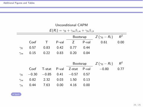
Unconditional CAPME(Ri) = “0 + “m—i,m + “h—i,h
Bootsrap Z (“0 ≠ Rf ) R2
Coef T P-val Z P-val 0.61 0.00“0 0.57 0.83 0.42 0.77 0.44“m 0.15 0.22 0.83 0.20 0.84
Bootsrap Z (“0 ≠ Rf ) R2
Coef T-stat P-val Z-stat P-val ≠0.80 0.77“0 ≠0.30 ≠0.85 0.41 ≠0.57 0.57“m 0.82 2.32 0.03 1.50 0.13“h 0.44 7.63 0.00 4.16 0.00
back
25 / 25
Additional Figures and Tables
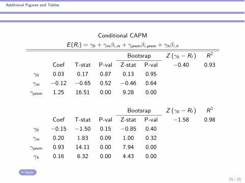
Conditional CAPME(Ri) = “0 + “m—i,m + “prem—i,prem + “h—i,h
Bootsrap Z (“0 ≠ Rf ) R2
Coef T-stat P-val Z-stat P-val ≠0.40 0.93“0 0.03 0.17 0.87 0.13 0.95“m ≠0.12 ≠0.65 0.52 ≠0.46 0.64
“prem 1.25 16.51 0.00 9.28 0.00
Bootsrap Z (“0 ≠ Rf ) R2
Coef T-stat P-val Z-stat P-val ≠1.58 0.98“0 ≠0.15 ≠1.50 0.15 ≠0.85 0.40“m 0.20 1.83 0.09 1.00 0.32
“prem 0.93 14.11 0.00 7.94 0.00“h 0.16 6.32 0.00 4.43 0.00
back25 / 25
Additional Figures and Tables
.4.6
.81
1.2
1.4
Re
aliz
ed
Ave
rag
e R
etu
rn (
%)
.4 .6 .8 1 1.2Predicted Expected Return (%)
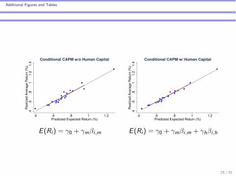
Conditional CAPM w/o Human Capital
.4.6
.81
1.2
1.4
Re
aliz
ed
Ave
rag
e R
etu
rn (
%)
.4 .6 .8 1 1.2Predicted Expected Return (%)
Conditional CAPM w/ Human Capital
E (Ri) = “0 + “m—i ,m E (Ri) = “0 + “m—i ,m + “h—i ,h
25 / 25

Additional Figures and Tables
5 10 15 20 25
!0.03
!0.02
!0.01
0.01
0.02
0.03
Relative BE!ME :
1
qA !1
qB
" dZA" dZB
5 10 15 20 25
!0.5
0.5
1.0!""
Expected Excess Return :
Et!dRA" ! Et!dRB"
# dZA # dZB
5 10 15 20 25
!4
!2
2
4
6
!""
Investment!to!Human
Capital Ratio : ΙH
5 10 15 20 25
!0.10
!0.05
0.05
0.10
0.15
!""
Consumption!to!Total
Capital Ratio : c
back
25 / 25

Additional Figures and Tables
5 10 15 20 25
!6
!4
!2
2
4
6
!""
Investment!to!Physical
Capital Ratio : ΙA
5 10 15 20 25
!5
5
10!""
Investment!to!Physical
Capital Ratio : ΙB
5 10 15 20 25
!4
!2
2
4
6
!""
Investment!to!Human
Capital Ratio : ΙH
5 10 15 20 25
!0.10
!0.05
0.05
0.10
0.15
!""
Consumption!to!Total
Capital Ratio : c
+dZ A
+dZ B
25 / 25
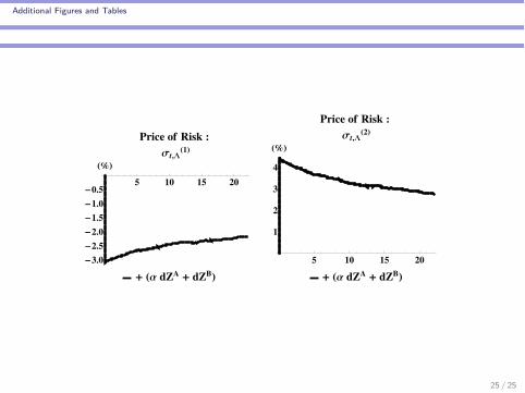
Additional Figures and Tables
5 10 15 20
!3.0
!2.5
!2.0
!1.5
!1.0
!0.5
!""
Price of Risk :
Σt,$!1"
% !Α dZA % dZB"
5 10 15 20
1
2
3
4
!!"
Price of Risk :
Σt,#!2"
$ !Α dZA $ dZB"
25 / 25
Additional Figures and Tables
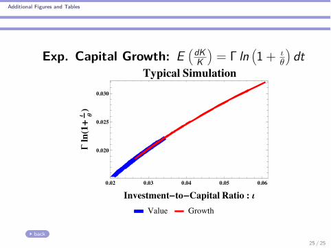
Exp. Capital Growth: E1dK
K2= � ln
11 + ÿ
◊
2dt
0.02 0.03 0.04 0.05 0.06
0.020
0.025
0.030
Investment-to-Capital Ratio : i
GlnH1+
i qLTypical Simulation
Value Growth
back25 / 25

Additional Figures and Tables
BE/ME: 1q = �
ÿ+◊
0.02 0.03 0.04 0.05 0.06
0.35
0.40
0.45
0.50
0.55
Investment-to-Capital Ratio : i
BEêME
Ratio:1 q
Typical Simulation
Value Growth
back25 / 25

Appendix
To calculate the returns on the Value and Growth stocks I merge monthlyreturns data from CRSP with fundamentals data from Compustat for the years1963-2012. Following the approach of Fama and French (1993 and 1996), Iform Value and Growth portfolios using the top thirtieth and the bottomthirtieth percentiles of BE/ME distributions with the BE/ME cut-o�s from theKenneth R. French Data Library.
BE is the sum of book equity, deferred taxes, and investment tax credit, minusthe book value of preferred stock for fiscal year t ≠ 1. ME is the value ofcommon equity at the end of year t ≠ 1. I then calculate returns from July ofyear t through June of year t + 1.
The mean return shown in the tables for the Value and Growth portfolios is theannualized average monthly returns. I multiply the average monthly return bytwelve and the standard deviation by the square-root of twelve.
I adjust the security returns for inflation using the GDP deflator. I use atwo-year rolling geometric average of the GDP deflator. I do so because Icalculate the security returns in data from July through June as done in Famaand French (1993; 1996). back
25 / 25
Appendix
The model is consistent with a setting where agents can invest inhuman capital by acquiring more schooling.
The adjustment cost for human capital may reflect someopportunity cost of time spent on schooling (as a means ofinvesting in human capital), psychic costs, or a reduction of thetime spent on leisure activities that are valuable to agents
The adjustment cost for physical capital may reflect some frictionsto capital reallocation, installation costs, or more general forms ofcapital illiquidity
In the model adj. costs are necessary for time-varying BE/ME andto ensure that both types of firms co-exist in equilibrium
back
25 / 25
Appendix
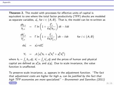
Theorem 2. The model with processes for e�ective units of capital isequivalent to one where the total factor productivity (TFP) shocks are modeledas separate variables, ai
t , for i œ {A, B}. That is, the model can be re-written asdhj,thj,t
= � ln3
1 +Ihj,t
◊aAt hj,t
4dt ≠ ”dt
dk ij,t
k ij,t
= � ln3
1 +I ij,t
◊aitk i
j,t
4dt ≠ ”dt for i œ {A, B}
dait = ai
t‡dZ it
Yt = A!aA
t ht + aAt kA
t + aBt kB
t"
where ht =s
J hj,tdj, k it =
sJ k i
j,tdj and the prices of human and physicalcapital are defined as aA
t pt and aitqi
t . Due to scale invariance, the valuefunction is una�ected.
To preserve scale invariance, at appears in the adjustment function. “The factthat adjustment costs are higher for high at can be justified by the fact thathigh TFP economies are more specialized.” – Brunnemeir and Sannikov (2011)
back 25 / 25
Appendix
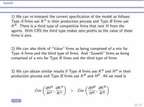
1) We can re-interpret the current specification of the model as follows:Type A firms use KA in their production process and Type B firms useKB . There is a third type of competitive firms that rent H from theagents. With CRS the third type makes zero profits so the value of thesefirms is zero.
2) We can also think of “Value” firms as being comprised of a mix forType A firms and the third type of firms. And “Growth” firms as beingcomprised of a mix for Type B firms and the third type of firms
3) We can obtain similar results if Type A firms use KA and HA in theirproduction process and Type B firms use KB and HB . All we need is
Cov3
dHA
HA ,dKA
KA
4> Cov
3dHB
HB ,dKB
KB
4
back25 / 25

Appendix
There are 2 state variables, x it =
Kit
Ht+KA+KB for i œ {A, B}.
We can write the value function as
V)
H + KA + KB , xA, xB*=
11 ≠ “
!!H + KA + KB"
F)
xA, xB*"1≠“
The Hamiltonian-Jacobi-Bellman (HJB) equation is
0 = maxIA,IB ,IH
f {C , V } dt + VHE (dH)
+VAE!dKA"
+ VBE!dKB"
+12
1VAA
!dKA"2
+ VBB!dKB"2
+ VHH (dH)2 + 2VAHdHdKA2
dH, dKA, dKB are given by the pre-specified LOM’sE (dH), E (dKA), and E (dKB) are the drifts and
Ct = Yt ≠!IAt + IB
t + IHt
"
Solution (back)
25 / 25

Appendix
Let c = CH+KA+KB , ÿi = I i
K i , and ÿH = IH
H . Following Eberly and Wang (2009;2011), c, ÿi , ÿH and F jointly solve
Resource constraint: c = A ≠ xAÿA ≠ xBÿB ≠ (1 ≠ xA ≠ xB)ÿH
FOC’s for IA, IB , IH : c = F
A�
!≠xAFA ≠ xBFB + F
"
— (ÿH + ◊)
B 1fl≠1
c = F
A�
!≠(xA ≠ 1)FA ≠ xBFB + F
"
— (ÿA + ◊)
B 1fl≠1
c = F
A�
!≠xAFA ≠ (xB ≠ 1)FB + F
"
— (ÿB + ◊)
B 1fl≠1
where F)
xA, xB*also solves the PDE in the 2 states obtained by simplifying
the HJB; with boundary conditions F {1, 0} = F {0, 1} = F and F {0, 0} = F .PDE Boundary Conditions Projection Method back to Implementation
25 / 25

Appendix
1. Re-write the state variables as {xA, xB}, functions of Chebyshev nodes.
2. Approximate F{xA, xB} with a complete Chebyshev polynomial,F{xA, xB}. The approximation function will be composed of completeorthogonal basis functions.
3. Define the residual function, R, as the PDE where we plug in theapproximation F and the as well as the nodes
)xA, xB*
.
4. Using the collocation approach, the vector of polynomial coe�cients –, ischosen to solve R {–} = 0 on the grid
)xA, xB*
. First choose the size ofthe n ◊ n grid. Then start with low order polynomials and solve for –.
5. Use an interpolation method to obtain the solution for F)
xA, xB*over
the continuous state space)
xA œ [0, 1], xB œ [0, 1 ≠ xA]*
. Plug thisfunction, F
)xA, xB*
, back into the PDE and examine the size of thePDE errors over the continuous state space.
6. Steadily increase the degree of the polynomial and repeat the procedureuntil the PDE errors are minimized.
back to Solution back to Implementation25 / 25
Appendix
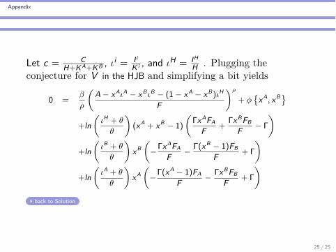
Let c = CH+KA+KB , ÿi = I i
K i , and ÿH = IHH . Plugging the
conjecture for V in the HJB and simplifying a bit yields
0 =—fl
3A ≠ xAÿA ≠ xBÿB ≠ (1 ≠ xA ≠ xB)ÿH
F
4fl
+ „)
xA, xB*
+ln3
ÿH + ◊◊
4(xA + xB ≠ 1)
3�xAFA
F +�xBFB
F ≠ �
4
+ln3
ÿB + ◊◊
4xB
3≠�xAFA
F ≠ �(xB ≠ 1)FBF + �
4
+ln3
ÿA + ◊◊
4xA
3≠�(xA ≠ 1)FA
F ≠ �xBFBF + �
4
back to Solution
25 / 25

Appendix
There are 3 boundary cases:{xA = 1 , xB = 1 , 1 ≠ xA ≠ xB = 1}.
I first solve the model for these 3 cases. I then use Projections Methodsfrom Judd (1998) and approximate F
)xA, xB*
with a completeChebyshev polynomial of degree 20, F , in {xA, xB}.
I solve for the coe�cients of the polynomial which jointly satisfy thefollowing conditions:
1) F{xA, xB} solves the HJB,2) F{xA, xB} satisfies the 3 boundary cases and,3) FOC’s for ÿA, ÿB , ÿH and resource the constraint are satisfied
back to Implementation back to Solution CES Di�culties
25 / 25

Appendix
Proposition 1We can decentralize the planner’s problem as follows.1) Agent endowed with H0, takes wage rate Êt , price of human capital pt , andinitial financial wealth W0 as given. Agent has access to a risk-less bond withreturn rt and a risky claims. Risky security prices: St = {S(A)
t , S(B)t }
Õ follows
dSt =1
µÕ
t diag (St) ≠ Dt2
dt +A
S(A)t ÎAÕ
tS(B)
t ÎBÕ
t
BdZt
The agent solves
max{Cj,t ,IH
j,t ,Hj,t ,Èj,t }Œt=0
E0
⁄ Œ
0f (Cj,t , Vj,t) dt s.t.:
dWj,t =!Wj,trt + Èj,t · Wj,t(µt ≠ 1rt) ≠ Cj,t ≠ IH
j,t + ÊtHj,t"
dt + ÈÕj,tWj,tÎtdZt
dHj,t/Hj,t = � ln3
1 +IHj,t
◊Hj,t
4dt ≠ ”dt + ‡hdZ A
t
Èj,t = {ÈAj,t , ÈB
j,t}Õ : fraction of Wj,t invested in risky securitiesand Ît is a 2 ◊ 2 matrix Proposition 1 Summary
25 / 25
Appendix
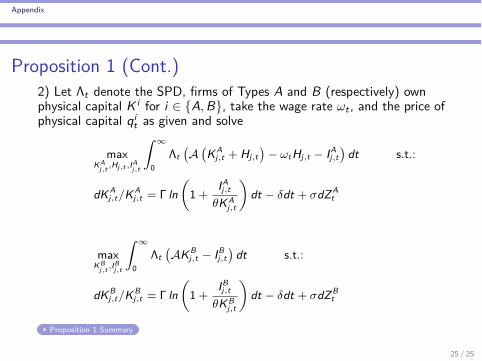
Proposition 1 (Cont.)2) Let ⇤t denote the SPD, firms of Types A and B (respectively) ownphysical capital K i for i œ {A, B}, take the wage rate Êt , and the price ofphysical capital qi
t as given and solve
maxKA
j,t ,Hj,t ,IAj,t
⁄ Œ
0⇤t
!A
!KA
j,t + Hj,t"
≠ ÊtHj,t ≠ IAj,t
"dt s.t.:
dKAj,t/KA
j,t = � ln3
1 +IAj,t
◊KAj,t
4dt ≠ ”dt + ‡dZ A
t
maxKB
j,t ,IBj,t
⁄ Œ
0⇤t
!AKB
j,t ≠ IBj,t
"dt s.t.:
dKBj,t/KB
j,t = � ln3
1 +IBj,t
◊KBj,t
4dt ≠ ”dt + ‡dZ B
t
Proposition 1 Summary
25 / 25
Appendix
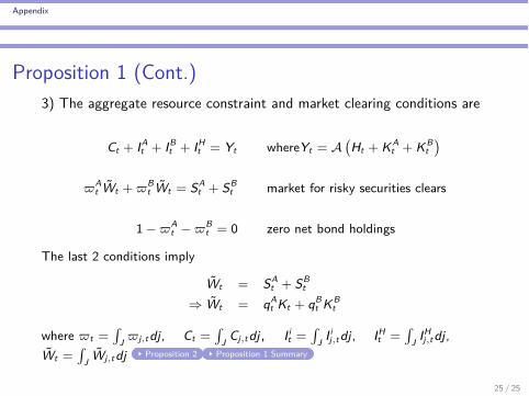
Proposition 1 (Cont.)3) The aggregate resource constraint and market clearing conditions are
Ct + IAt + IB
t + IHt = Yt whereYt = A
!Ht + KA
t + KBt
"
ÈAt Wt + ÈB
t Wt = SAt + SB
t market for risky securities clears
1 ≠ ÈAt ≠ ÈB
t = 0 zero net bond holdings
The last 2 conditions imply
Wt = SAt + SB
t
∆ Wt = qAt Kt + qB
t KBt
where Èt =s
J Èj,tdj, Ct =s
J Cj,tdj, I it =
sJ I i
j,tdj, IHt =
sJ IH
j,tdj,Wt =
sJ Wj,tdj Proposition 2 Proposition 1 Summary
25 / 25

Appendix
Ct + IAt + IB
t + IHt = Yt whereYt = A
!Ht + KA
t + KBt
"
ÈAt Wt + ÈB
t Wt = SAt + SB
t market for risky securities clears1 ≠ ÈA
t ≠ ÈBt = 0 zero net bond holdings
The last 2 conditions implyWt = SA
t + SBt
∆ Wt = qAt Kt + qB
t KBt
Using the static constraint
Wt = Et
⁄ Œ
t
⇤s⇤t
!Cs + IH
s ≠ ÊsHs"
ds
Using SHt = ptHt = Et
s Œt
⇤s⇤t
!AHs ≠ IH
s"
ds (given by FOCs and Prop. 2)back Proposition 2
Et
⁄ Œ
t
⇤s⇤t
!Cs + IH
s ≠ ÊsHs"
ds = qAt Kt + qB
t KBt
∆ Et
⁄ Œ
t
⇤s⇤t
Cs ds = ptHt + qAt Kt + qB
t KBt as expected
25 / 25
Appendix
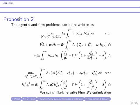
Proposition 2The agent’s and firm problems can be re-written as
max{Cj,t ,IH
j,t ,Hj,t }Œt=0
E0
⁄ Œ
0f (Cj,t , Vj,t) dt s.t.:
W0 + p0H0 = E0
⁄ Œ
0⇤t
!Cj,t + IH
j,t ≠ ÊtHj,t"
dt
+E0
⁄ Œ
0⇤tptHj,t
3Âtpt
≠ � ln3
1 +IHj,t
◊Hj,t
4+ ”
4dt
maxKA
j,t ,Hj,t ,IAj,t
⁄ Œ
0⇤t
!A
!KA
j,t + Hj,t"
≠ ÊtHj,t ≠ IAj,t
"dt s.t.:
KA0 qA
0 = E0
⁄ Œ
0⇤tqA
t KAj,t
3ÂA
tqA
t≠ � ln
31 +
IAj,t
◊KAj,t
4+ ”
4dt
We can similarly re-write Firm B’s optimizationProof {Ât , Âi
t } Market Clearing and Resource Constraint Proposition 1 (cont.)25 / 25
Appendix
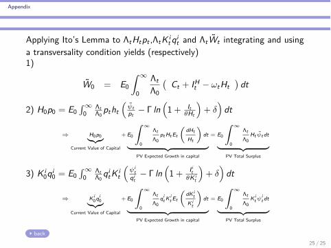
Applying Ito’s Lemma to ⇤tHtpt ,⇤tK it qi
t and ⇤tWt integrating and usinga transversality condition yields (respectively)1)
W0 = E0
⁄ Œ
0
⇤t⇤0
!Ct + IH
t ≠ ÊtHt"
dt
2) H0p0 = E0s Œ
0⇤t⇤0
ptht1
Âtpt
≠ � ln1
1 + It◊Ht
2+ ”
2dt
∆ H0p0¸˚˙˝Current Value of Capital
+ E0
⁄ Œ
0
⇤t⇤0
pt Ht Et
1dHtHt
2dt
¸ ˚˙ ˝PV Expected Growth in capital
= E0
⁄ Œ
0
⇤t⇤0
Ht Ât dt
¸ ˚˙ ˝PV Total Surplus
3) K i0qi
0 = E0s Œ
0⇤t⇤0
qitK i
t
1Âi
tqi
t≠ � ln
11 + I i
t◊Ki
t
2+ ”
2dt
∆ Ki0qi
0¸˚˙˝Current Value of Capital
+ E0
⁄ Œ
0
⇤t⇤0
qit K i
t Et
1dKi
tK i
t
2dt
¸ ˚˙ ˝PV Expected Growth in capital
= E0
⁄ Œ
0
⇤t⇤0
Kit Âi
t dt
¸ ˚˙ ˝PV Total Surplus
back25 / 25

Appendix
Ât © pt
1≠Et
Ëd(⇤tpt)
⇤tpt
È+ ‡h‡
(A)⇤,t
2
Âit © qi
t
3≠Et
5d(⇤tqi
t)
⇤tqit
6+ ‡‡
(i)⇤,i,t
4
‡⇤,t = {‡(A)⇤,t , ‡
(B)⇤,t }
Õ= Di�usion
Ëd(⇤tpt)
⇤tpt
È
‡⇤,i,t = {‡(A)⇤,i,t , ‡
(B)⇤,i,t}
Õ= Di�usion
5d(⇤tqi
t)
⇤tqit
6
In equilibrium we have
FOC for Cand H: Ât = Êt¸˚˙˝marginal benefit from human capital
≠1
≠pt
1� ln
1pt
�
◊
2≠ ”
2+ pt� ≠ ◊
2
¸ ˚˙ ˝marginal cost to human capital
FOC for Ki : Âit = A¸˚˙˝
marginal product of physical capital
≠1
≠qit
1� ln
1qi
t�
◊
2≠ ”
2+ qi
t� ≠ ◊
2
¸ ˚˙ ˝marginal cost to physical capital
back to Prop2 back to AP25 / 25
Appendix
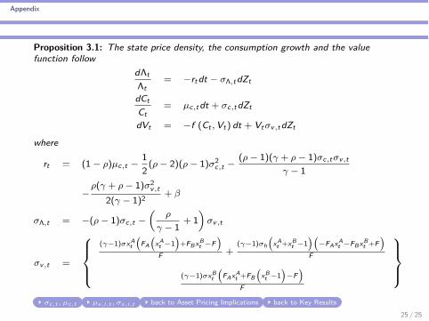
Proposition 3.1: The state price density, the consumption growth and the valuefunction follow
d⇤t⇤t
= ≠rtdt ≠ ‡⇤,tdZt
dCtCt
= µc,tdt + ‡c,tdZt
dVt = ≠f (Ct , Vt) dt + Vt‡v,tdZt
where
rt = (1 ≠ fl)µc,t ≠12(fl ≠ 2)(fl ≠ 1)‡2
c,t ≠(fl ≠ 1)(“ + fl ≠ 1)‡c,t‡v,t
“ ≠ 1
≠fl(“ + fl ≠ 1)‡2
v,t2(“ ≠ 1)2 + —
‡⇤,t = ≠(fl ≠ 1)‡c,t ≠1
fl
“ ≠ 1+ 1
2‡v,t
‡v,t =
Y_]
_[
(“≠1)‡xAt!
FA!
xAt ≠1
"+FBxB
t ≠F"
F +(“≠1)‡h
!xA
t +xBt ≠1
"!≠FAxA
t ≠FBxBt +F
"
F
(“≠1)‡xBt!
FAxAt +FB
!xB
t ≠1"
≠F"
F
Z_
_\
‡c,t , µc,t µx,i,t , ‡x,i,t back to Asset Pricing Implications back to Key Results25 / 25

Appendix
Ct = A!
Ht + KAt + KB
t"
≠ Ht!�pt
)xA
t , xBt
*≠ ◊
"≠ KA
t!�qA
t)
xAt , xB
t*
≠ ◊"
≠KBt
!�qB
t)
xAt , xB
t*
≠ ◊"
Using Ito’s Lemma
µc,t =1Ct
Q
ccca
ˆCtˆHt
◊ Ht
1� ln
11 +
IHt
◊Ht
2≠ ”
2+ 1
2ˆ2CtˆH2
t◊ Ht‡2
h + ˆ2CtˆHt ˆKA
t◊ HtKA
t ‡‡h
+ ˆCtˆKA
t◊ KA
t
1� ln
11 +
IAt
◊KAt
2≠ ”
2+ 1
2ˆ2Ct
ˆ(KAt )
2 ◊ KAt ‡2
+ ˆCtˆKB
t◊ KB
t
1� ln
11 +
IBt
◊KBt
2≠ ”
2+ 1
2ˆ2Ct
ˆ(KBt )
2 ◊ KBt ‡2
R
dddb
‡c,t =1Ct
;ˆCtˆHt
◊ Ht‡h +ˆCtˆKA
t◊ KA
t ‡ ,ˆCtˆKB
t◊ KB
t ‡
<
SPD Formulas back to Asset Pricing Implications
25 / 25

Appendix
dxit = µx,i,tdt + ‡
Õx,i,tdZt
µx,A,t = xA
Q
ccccca
‡2h!
xA + xB ≠ 1"2 ≠ ‡
!2xA ≠ 1
"‡h
!xA + xB ≠ 1
"
+‡21!
xA ≠ 1"
xA +!
xB"2
2
+�!
xA + xB ≠ 1"
ln!�pt◊
"+
!� ≠ �xA
"ln
1�qA
◊
2
≠�xB ln1
�qB
◊
2
R
dddddb
‡x,A,t =)
xA !‡h
!xA + xB ≠ 1
"+ ‡
!1 ≠ xA""
, ≠‡xAxB*
µx,B,t = xB
Q
ccccca
≠2‡xA‡h!
xA + xB ≠ 1"+ ‡2
h!
xA + xB ≠ 1"2
+‡21!
xA"2
+!
xB ≠ 1"
xB2
+�!
xA + xB ≠ 1"
ln!�pt◊
"≠ �xA ln
1�qA
◊
2
+!� ≠ �xB
"ln
1�qB
◊
2
R
dddddb
‡x,B,t =)
xB !‡h
!xA + xB ≠ 1
"≠ ‡xA"
, ≠‡xB !xB ≠ 1
"*
back to SPD formulas back to Asset Pricing Implications 25 / 25

Appendix
dRm = dRA qAKA
qAKA + qBKB + dRB qBKB
qAKA + qBKB
dRw =
Q
cadRH pH
pH+qAKA+qBKB + dRA qAKA
pH+qAKA+qBKB
+dRB qBKB
pH+qAKA+qBKB
R
db
back
25 / 25
Appendix
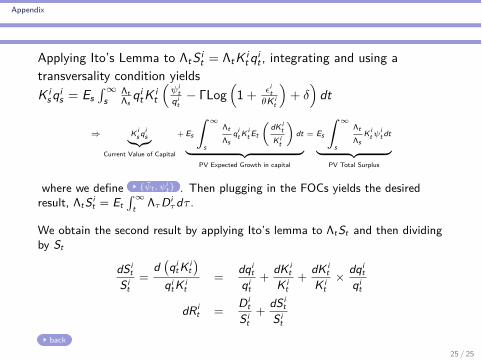
Applying Ito’s Lemma to ⇤tS it = ⇤tK i
t qit , integrating and using a
transversality condition yieldsK i
s qis = Es
s Œs
⇤t⇤s
qitK i
t
1Âi
tqi
t≠ �Log
11 + ‘i
t◊Ki
t
2+ ”
2dt
∆ Kis qi
s¸˚˙˝Current Value of Capital
+ Es
⁄ Œ
s
⇤t⇤s
qit K i
t Et
1dKi
tK i
t
2dt
¸ ˚˙ ˝PV Expected Growth in capital
= Es
⁄ Œ
s
⇤t⇤s
K it Âi
t dt
¸ ˚˙ ˝PV Total Surplus
where we define {Ât , Âit } . Then plugging in the FOCs yields the desired
result, ⇤tS it = Et
s Œt ⇤· Di
· d· .
We obtain the second result by applying Ito’s lemma to ⇤tSt and then dividingby St
dS it
S it
=d
!qi
tK it"
qitK i
t=
dqit
qit+
dK it
K it
+dK i
tK i
t◊ dqi
tqi
t
dR it =
Dit
S it+
dS it
S it
back25 / 25
Appendix
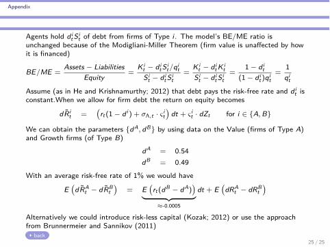
Agents hold dit Si
t of debt from firms of Type i . The model’s BE/ME ratio isunchanged because of the Modigliani-Miller Theorem (firm value is una�ected by howit is financed)
BE/ME =Assets ≠ Liabilities
Equity=
Kit ≠ di
t Sit/qi
tSi
t ≠ dit Si
t=
Kit ≠ di
t K it
Sit ≠ di
t Sit
=1 ≠ di
t(1 ≠ di
t)qit=
1qi
t
Assume (as in He and Krishnamurthy; 2012) that debt pays the risk-free rate and dit is
constant.When we allow for firm debt the return on equity becomes
dRit =
!rt(1 ≠ di ) + ‡⇤,t · Î i
t"
dt + Î it · dZt for i œ {A, B}
We can obtain the parameters {dA, dB} by using data on the Value (firms of Type A)and Growth firms (of Type B)
dA = 0.54dB = 0.49
With an average risk-free rate of 1% we would have
E!
dRAt ≠ dRB
t"
= E!
rt(dB ≠ dA)"
¸ ˚˙ ˝¥-0.0005
dt + E!
dRAt ≠ dRB
t"
Alternatively we could introduce risk-less capital (Kozak; 2012) or use the approachfrom Brunnermeier and Sannikov (2011)
back25 / 25
Appendix
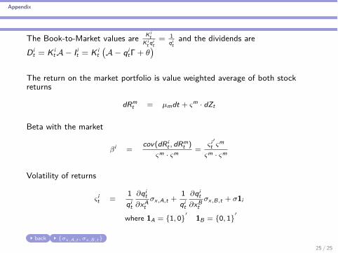
The Book-to-Market values are Kit
Kit qi
t= 1
qit
and the dividends areDi
t = K it A ≠ I i
t = K it!A ≠ qi
t�+ ◊"
The return on the market portfolio is value weighted average of both stockreturns
dRmt = µmdt + Îm · dZt
Beta with the market
—i =cov(dRi
t , dRmt )
Îm · Îm =Î iÕt Îm
Îm · Îm
Volatility of returns
Î it =
1qi
t
ˆqit
ˆxAt
‡x,A,t +1qi
t
ˆqit
ˆxBt
‡x,B,t + ‡1i
where 1A = {1, 0}Õ
1B = {0, 1}Õ
back {‡x,A,t , ‡x,B,t }
25 / 25

Appendix
Set — = —, ” = 0, � = ◊, and ‡ = ‡h.
Search for 7 unknowns {◊, A, cú, F ú, “, fl, ‡} to solve 7 equations:I In a 1-capital economy: 1) output growth of 2% , 2) C
Y of 90%, 3)resource constraint, 4) FOC for investment, 5) HJB
I 6) risk-free rate of 0.90%, 7) volatility of market portfolio of 16%Note: there is no gov’t exp. so C/Y is higher than in data
CalibrationVariable Name/Calculation Value
A Marginal Product of Capital 20.63%cú Consumption
Capital in one-capital economy 18.63%F ú Normalized Value Function, F , in one-capital economy 0.0791“ Risk Aversion Parameter 3.97
� = ◊ Adjustment Cost Parameters 2.73%fl Implied IES Parameter = 2.0025 0.5006
‡ = ‡h Standard deviation of Capital Growth 21.27%back Alternative Calibration
25 / 25
Appendix
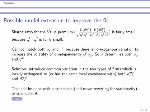
Possible model extension to improve the fit
Sharpe ratio for the Value premium ( Et(dRAt )≠Et(dRB
t )ÔÎA
t ·ÎAt ≠2ÎA
t ·ÎBt +ÎB
t ·ÎBt
) is fairly small
because ÎAt · ÎB
t is fairly small.
Cannot match both ‡y and Îm because there is no exogenous variation toincrease the volatility of q independently of ‡y . So ‡ determines both ‡yand Îm
Solution: introduce common variation in the two types of firms which islocally orthogonal to (or has the same local covariance with) both dZA
tand dZB
t .
This can be done with “ stochastic (and mean reverting for stationarity),or stochastic ◊.
back
25 / 25

Appendix
Impulse Responses
Let ‰t denote a given endogenous variable of the model. Following Koop,Pesaran and Potter (1996) and Kozak (2012), I construct two non-linearimpulse responses for ‰t using
IRF‰
)xA
t , xBt
*= E
1‰t
---xA0 = xA, xB
0 = xB , dZ0 = 1i
2
1i œÓ
{1, 0}Õ, {0, 1}
Õ, {0.5, 1}
ÕÔ
Thus, starting at the mean values for the state variables {xA, xB}, I introduce aone-standard-deviation positive shock through dZ A or dZ B or both at date zeroand simulate twenty-five years of observations one-hundred-thousand times. Ithen compute the average across simulations. I define the impulse responserelative to a baseline with no shock at date zero. back
25 / 25

Appendix
Properties of the Equilibrium
qit depends on states and the firm type. pt depends on states
In equilibrium, H and K i follow
dHt = Ht
1� ln
1pt
�◊
2≠ ”
2dt + Ht‡hdZ A
t
dK it = K i
t
1� ln
1qi
t�◊
2≠ ”
2dt + K i
t ‡dZ it
25 / 25
Appendix
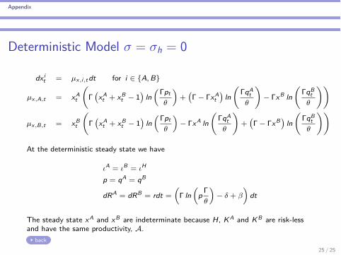
Deterministic Model ‡ = ‡h = 0
dxit = µx,i,tdt for i œ {A, B}
µx,A,t = xAt
3�
!xA
t + xBt ≠ 1
"ln
1�pt◊
2+
!� ≠ �xA
t"
ln3
�qAt
◊
4≠ �xB ln
3�qB
t◊
44
µx,B,t = xBt
3�
!xA
t + xBt ≠ 1
"ln
1�pt◊
2≠ �xA ln
3�qA
t◊
4+
!� ≠ �xB"
ln3
�qBt
◊
44
At the deterministic steady state we have
ÿA = ÿB = ÿH
p = qA = qB
dRA = dRB = rdt =1� ln
1p �
◊
2≠ ” + —
2dt
The steady state xA and xB are indeterminate because H, KA and KB are risk-lessand have the same productivity, A.
back25 / 25
Appendix
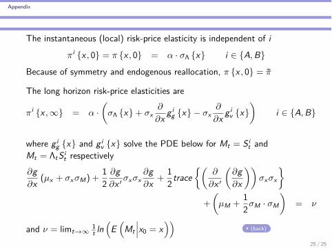
The instantaneous (local) risk-price elasticity is independent of i
fii {x , 0} = fi {x , 0} = – · ‡⇤ {x} i œ {A, B}
Because of symmetry and endogenous reallocation, fi {x , 0} = fi
The long horizon risk-price elasticities are
fii {x , Œ} = – ·3
‡⇤ {x} + ‡xˆ
ˆx g ig {x} ≠ ‡x
ˆ
ˆx g iv {x}
4i œ {A, B}
where g ig {x} and g i
v {x} solve the PDE below for Mt = S it and
Mt = ⇤tS it respectively
ˆgˆx (µx + ‡x ‡M) +
12
ˆgˆx Õ ‡x ‡x
ˆgˆx +
12 trace
;3ˆ
ˆx Õ
3ˆgˆx
44‡x ‡x
<
+
3µM +
12‡M · ‡M
4= ‹
and ‹ = limtæŒ1t ln
1E
1Mt
---x0 = x22
(back)
25 / 25

Appendix
Following Section 6.4 of Borovicka et al. (2011), the limiting Valuepremium is
limtæŒ
Y]
[
1t
Ëln
1E
1SA
t
---x0 = x22
≠ ln1
E1⇤tSA
t
---x0 = x22È
≠ 1t
Ëln
1E
1SB
t
---x0 = x22
≠ ln1
E1⇤tSB
t
---x0 = x22È
Z^
\ = “‡‡h
where ‡‡hdt = Cov1
dHH , dKA
KA
2≠ Cov
1dHH , dKB
KB
2
We are able to characterize the limiting Value premium by the product ofthe risk aversion governing parameter and the relative covariance ofhuman capital growth with the asset growth of Value firms.
(back)
25 / 25

Appendix
(back)
25 / 25

Appendix
!0.05 0.05 0.10 0.15 0.20 0.25
5
10
15
20
Distribution For Relative Risk!Price Elasticity
ΠA!x,#" ! ΠB!x,#"
E #ΠA !x, #" ! ΠB !x, #"$ $ 0.06
(back)
25 / 25
Appendix
5 10 15 20Τ
0.0018
0.0020
0.0022
0.0024
0.0026
0.0028
0.0030
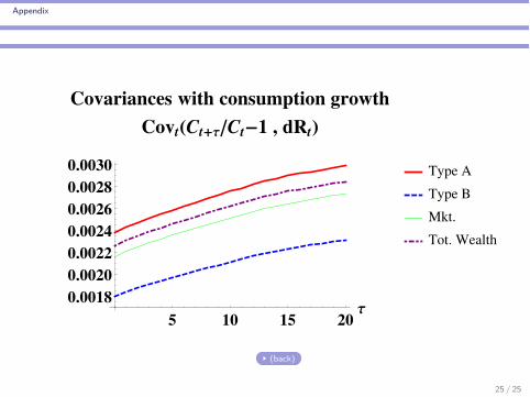
Covariances with consumption growth
Covt!Ct"Τ"Ct#1 , dRt#
Type A
Type B
Mkt.
Tot. Wealth
(back)
25 / 25

Appendix
5 10 15 20Τ
"0.2
0.2
0.4
0.6
0.8
1.0
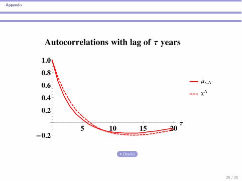
Autocorrelations with lag of Τ years
Μc
Et!dRA"
Et!dRB"
Et!dRm"
Et!dRw"
(back)
25 / 25
Appendix
5 10 15 20Τ
"0.2
0.2
0.4
0.6
0.8
1.0
Autocorrelations with lag of Τ years
Μx,A
xA
(back)
25 / 25
Appendix
5 10 15 20Τ
"0.2
0.2
0.4
0.6
0.8
1.0
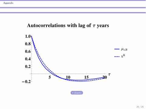
Autocorrelations with lag of Τ years
Μx,B
xB
(back)
25 / 25
Appendix
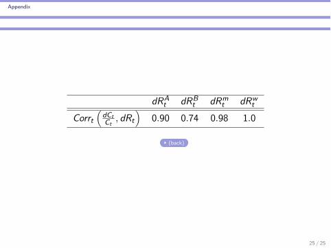
dRAt dRB
t dRmt dRw
t
Corrt1
dCtCt
, dRt2
0.90 0.74 0.98 1.0
(back)
25 / 25
Appendix
xA
xB
0.2 0.4 0.6 0.8 1.0
1
2
3
4
Distributions For State Variables
E !xA" ! 0.31
E !xB" ! 0.37
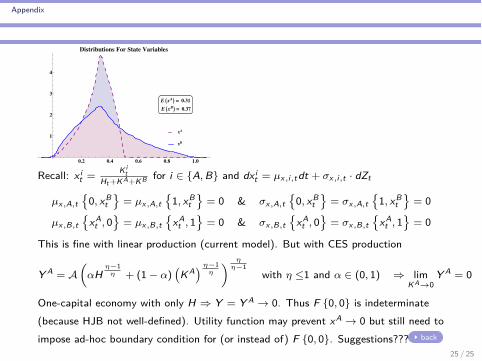
Recall: x it =
Kit
Ht+KA+KB for i œ {A, B} and dxit = µx,i,tdt + ‡x,i,t · dZt
µx,A,t)
0, xBt
*= µx,A,t
)1, xB
t*
= 0 & ‡x,A,t)
0, xBt
*= ‡x,A,t
)1, xB
t*
= 0
µx,B,t)
xAt , 0
*= µx,B,t
)xA
t , 1*
= 0 & ‡x,B,t)
xAt , 0
*= ‡x,B,t
)xA
t , 1*
= 0
This is fine with linear production (current model). But with CES production
Y A = A1
–H÷≠1
÷ + (1 ≠ –)!
KA" ÷≠1÷
2 ÷÷≠1
with ÷ Æ1 and – œ (0, 1) ∆ limKAæ0
Y A = 0
One-capital economy with only H ∆ Y = Y A æ 0. Thus F {0, 0} is indeterminate(because HJB not well-defined). Utility function may prevent xA æ 0 but still need toimpose ad-hoc boundary condition for (or instead of) F {0, 0}. Suggestions??? back
25 / 25

Appendix
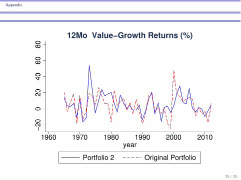
Constructing Modified HmL Portfolios
BE/ME Quintiles—h Quintiles Low 2 3 4 HighLow Short Short2 Short Short34 Long LongHigh Long Long
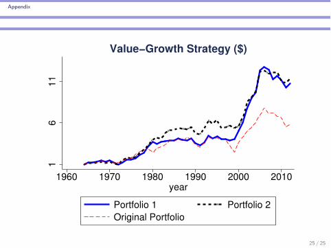
The modified HmL portfolios are long the Value portfolio and short the Growthportfolio. The Value portfolio is a value-weighted sum of securities in the cellslabelled “Long”. The Growth portfolio is a value-weighted sum of securities inthe cells labelled “Short”. Modified Portfolio 1 contains securities from all cellslabelled “Long” or “Short”. Modified Portfolio 2 contains only securitieslabelled in bold letters.
25 / 25
Appendix
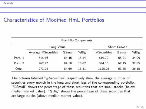
Characteristics of Modified HmL Portfolios
Portfolio Components
Long Value Short GrowthAverage #Securities %Small %Big #Securities %Small %Big
Port. 1 515.76 84.46 15.54 619.72 65.91 34.09Port. 2 267.27 84.18 15.82 324.10 67.15 32.85Orig. 973.08 84.69 15.31 1125.26 63.85 36.15
The column labelled “#Securities” respectively show the average number ofsecurities every month in the long and short legs of the corresponding portfolio.“%Small” shows the percentage of these securities that are small stocks (belowmedian market value). “%Big” shows the percentage of these securities thatare large stocks (above median market value).
25 / 25

Appendix
Performance of Modified HmL Portfolios
Portfolio Characteristics From Monthly Returns
Annualized (%) CAPM Results Correlations
E (R) ‡ (R) S.R. – — Port. 1 Port. 2 Orig. Mkt.
Port. 1 5.59 13.30 42.03 0.48 ≠0.03 1.00 0.89 0.54 ≠0.04
[3.00] [≠0.84]
Port. 2 5.70 13.37 42.63 0.51 ≠0.08 1.00 0.45 ≠0.10
[3.20] [≠2.29]
Orig. 4.08 10.60 38.49 0.38 ≠0.09 1.00 ≠0.13
[3.02] [≠3.23]
Mkt. 7.16 15.45 40.52 ≠ ≠ 1.00
Calculations are done with monthly portfolio returns. Returns are annualized bymultiplying the mean by 12 and the standard deviations by
Ô12.
25 / 25

Appendix
Portfolio Characteristics From Cumulative Annual Returns
(%) CAPM Results Correlations
E (Re ) ‡ (Re ) S.R. – — Port. 1 Port. 2 Orig. Mkt.
Port. 1 5.83 12.85 45.37 6.56 ≠0.14 1.00 0.83 0.62 ≠0.13
[10.82] [≠4.00]
Port. 2 5.94 13.13 45.24 7.39 ≠0.27 1.00 0.54 ≠0.31
[12.86] [≠8.28]
Orig. 4.70 14.15 33.22 5.83 ≠0.25 1.00 ≠0.29
[10.27] [≠7.87]
Mkt. 7.56 16.74 39.79 ≠ ≠ 1.00
Calculations are done with (twelve-month cumulative) annual portfolio returns.
25 / 25
Appendix
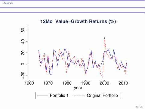
−2
00
20
40
60
1960 1970 1980 1990 2000 2010year
Portfolio 1 Original Portfolio
12Mo Value−Growth Returns (%)
25 / 25
Appendix
−2
00
20
40
60
80
1960 1970 1980 1990 2000 2010year
Portfolio 2 Original Portfolio
12Mo Value−Growth Returns (%)
25 / 25
Appendix
16
11
1960 1970 1980 1990 2000 2010year
Portfolio 1 Portfolio 2
Original Portfolio
Value−Growth Strategy ($)
25 / 25