Embed Size (px)
Citation preview

Master Programme in Finance
Does Hedging Increase Firm
Value?
An Examination of Swedish Companies
Author: Ngan Nguyen
Supervisor: Ph.D. Håkan Jankengård

ABSTRACT In an uncertain financial world, corporate risk management has become an important
element of a firm’s overall business strategy. The ability to manage risk will help
companies act more confidently on future business decisions. Their knowledge of the
risks they are facing will give them various options on how to deal with potential
problems. One of the most popular risk management programs that firm adopts is to
hedge against the future’s fluctuations of income due to the changes in currency
exchange rate or interest rate risk. Despite an increasing interest in developing theoretical
studies about the reasons why firms involved in risk management, however, only a
handful of studies that address the issue whether risk management can enhance the firm
value. The purpose of this project research is to fill this gap and investigate the impact of
hedging on firm value.
Using Tobin’s Q as an approximation for firm market value and hedging as a control
variable, I examined 90 Swedish firms listed on the Stockholm Stock Exchange, having
the total assets exceeds at least 1 billion Euros. The results of the regression analysis
show insignificant indication that the usage of hedging impacts firm value positively. The
findings of this research imply that there is no evidence that support the hypothesis that
hedging causes an increase in firm value.
Key words: corporate hedging, firm value, risk management, derivative

PREFACE
The past ten weeks writing this master thesis have been very interesting, educating and
challenging. Developing this thesis has been hard work and time- consuming nonetheless
a process of learning.
I would like to express my sincerest gratitude towards my supervisor, Ph.D., Assistant
Professor Håkan Jankengård for being a countless supportive person when developing
my thesis and for help me during the troublesome phase. Without his guidance, this thesis
would not be enabled.
Lund, May 2015

Table of Contents
1. INTRODUCTION ............................................................................................... 1 1.1 BACKGROUND ............................................................................................................................................. 1
1.2 PROBLEM DISCUSSION .............................................................................................................................. 3
1.4 AIM AND RESEARCH QUESTION .......................................................................................................... 4
1.5 LIMITATIONS .................................................................................................................................................... 5
1.6 RELEVANCE OF THE STUDY ................................................................................................................... 5
1.7 OUTLINE OF THE THESIS .......................................................................................................................... 5
2. LITERATURE REVIEW ................................................................................... 7 2.1 THE MODIGLIANI AND MILLER THEOREM ................................................................................... 7
2.2 THE THEORIES OF CAPITAL ASSET PRICING MODEL (CAPM) ........................................... 8
2.3 WHY FIRM HEDGE? .................................................................................................................................... 11
2.3.1 MINIMIZING THE UNDERINVESTMENT PROBLEM ................................................................ 11 2.3.2 MANAGERIAL RISK ADVERSION, COMPENSATION, AND HEDGING ........................... 12 2.3.3 DEBT AND HENDGING POLICIES ...................................................................................................... 13 2.3.4 TAX BENEFITS AND HEDGING POLICIES ..................................................................................... 15
2.4 SUMMARY .................................................................................................................................................. 17
3. METHODOLOGY .............................................................................................. 19 3.1 RESEARCH APPROACH AND STRATEGY ...................................................................................... 19
3.2 DATA COLLECTION ................................................................................................................................... 19
3.3 RESEARCH PROCEDURES ...................................................................................................................... 20
3.4 STATISTICAL DISTRIBUTIONS FOR DIAGNOTIC TESTS...................................................... 24
3.5 LIMITATION ................................................................................................................................................... 26
4. RESULTS AND ANALYSIS ............................................................................. 27 4.1 EMPIRICAL FINDINGS .............................................................................................................................. 27
4.1.1 STATISTICAL TEST ....................................................................................................................................... 27 4.1.2 HEDGING AND FIRM VALUE USING MULTIVARIATE TEST .......................................... 27 4.1.3 ROBUSTNESS .................................................................................................................................................. 28
4.2 ANALYSIS OF THE FINDINGS .............................................................................................................. 30
5. CONCLUSION ................................................................................................. 32
6. REFERENCES .................................................................................................... 33
7. APPENDIX ....................................................................................................... 37

1
1. INTRODUCTION
This chapter begins with a brief overview about the impact of hedging on firm value and the
reason firms hedge. The problem discussion will highlight the contradict findings related to
whether hedging impact firms value. Subsequently, I am presenting the aim and research
question at the end of the chapter.
1.1 BACKGROUND
Corporate risk management is an important element of a firm’s overall business strategy (Guay
& Kothari, 2002). In an uncertain financial world, a better understanding of the impact of risk
management on firm value is valuable to determine the firm’s long- term success. Stulz (1996)
argued that the primary goal of risk management is to eliminate the probability of costly lower-
tail outcomes- those that would cause financial distress or make a company unable to carry out
its investment strategy. In the last decades, risk management has moved from pure risk
mitigation to value creation (Ahmed, Azevedo & Guney, 2010). Despite the prevalence of
corporate risk management and the effort that has been devoted to develop theoretical studies
about the reasons why firms involved in risk management, however, only a handful of studies
that address the issue whether risk management can actually enhance the firm value (Haushalter,
2000; Allayannis & Weston, 2001).
As a definition of risk management, it is a process of thinking systematically about all possible
risks, problems or disasters before they happen and setting up procedures that will avoid risk or
at least minimize its impact1. The most popular risk management program that firms adopt is
hedging; a firm can hedge by trading in particular futures, forward or option market even though
it has no identifiable cash position in the underlying commodity (Smith & Stulz, 1985).
According to the classic Modigliani and Miller paradigm, in a perfect market, risk management
is irrelevant to firm as shareholders can do it on their own at the same cost (Yin & Jorion, 2004).
However, recent studies have shown that in the presence of realistic capital market
1 An Introduction to Risk Management, www.ourcommunity.com.au

2
imperfections, i.e. agency costs, costs of external financing, direct and indirect bankruptcy costs,
as well as taxes, corporate hedging will enhance the shareholder value (Hagelin, 2003; Aretz,
Bartram & Dufey, 2007). Those studies suggested that hedging could increase firms’ values by
reducing the expected costs of financial distress, lowering the expected cost of taxes or minimize
the underinvestment problems. Geczy, Minton and Schrand (1997) besides providing empirical
evidence and further theoretical arguments, which support the view, that hedging can create
value; they also found that firms’ use of currency derivatives is positively related to growth
opportunities by examining currency-hedging activities for a large sample of Fortune 500 firms.
Allayannis and Weston (2001) studied the relationship between hedging and firm value, with a
sample of 720 firms, the authors focus their analysis on the subsample of firms that are exposed
to exchange rate risk through sales from foreign operations and examine whether firms that have
similar exposure differ in value, depending on whether they hedge or not. The finding of their
studies indicates that firms that begin a hedging policy experience an increase in value relative to
those firms that choose to remain unhedged and that firms that quit hedging experience a
decrease in value relative to those firms that choose to remain hedged. Ahmed, Azevedo and
Guney (2010) by studying a sample of 288 nonfinancial UK firms, also found evidence that
support the value creating theory. Although the effect of hedging on firm value and performance
varies significantly across financial risks and that there are derivatives that are more effective in
hedging certain types of risks, contributing favorably to value creation and financial perform.
Similarly, Jankengard (2015) by studying the sample of 257 listed Swedish firms found
evidences consistent with the hypothesis that derivatives usage is more value creating in firms
with centralized FX exposure management than in firms with a decentralized approach.
While all of the risk management theories indicated that hedging could increase firm value, the
type of firm risk targeted by theories varies. For example, if a firm faces costly external
financing then the focus will lay on the volatility of cash flows as the risk measure to be hedged.
On the other hand, when the firms’ managers are risk adverse and under- diversified with respect
to their compensation, they are likely to reduce the firm’s risk by hedging in order to reduce the
required risk premium. In the case, the type of risk targeted for hedging is associated with cash
flows, earnings, or stock price volatility, depending on the nature of the managers’ compensation

3
contract and firm- specific wealth (Guay & Kothari, 2002). Another incentive for firms to hedge
is to reduce the expected cost of tax liability. The structure of the tax code can make it
advantageous for firms to take positions in futures, forward, or options markets. If effective
marginal tax rates are an increasing function of the corporation’s pre- tax value. If hedging
reduces the variability of pre –tax value, then the expected corporate tax liability is reduced and
the expected post- tax value of the firm is increased, as long as the cost of the hedge is not too
large (Smith & Stulz, 1985).
1.2 PROBLEM DISCUSSION
There is mixed support for value creating theories; however, it could be argued that corporate
hedging has no impact on firm value (Modigliani & Miller, 1958), as investors can achieve risk
reduction at least as efficiently themselves through diversification. Dufey and Srinivasulu (1983)
argued that the hedging of risks that investors cannot diversify in financial markets might also
not increase shareholder value, as investors receive an appropriate return for holding securities of
inherently risky businesses. Therefore, corporate hedging of market risks simply shifts firms
along a line that reflect the risk/reward tradeoff in the market. Mian (1996) surveyed the effect of
hedging activities on gold mining firms and found no support for the value maximization theory
even though he found strong evidence that supported the managerial risk aversion theory:
according to which managers who hold more stock tend to undertake more hedging activities. Jin
and Jorion (2006) investigated the hedging activities of a sample of 119 U.S oil and gas
producers from 1998 to 2001. They tested for a difference in firm value between firms that hedge
and those that do not hedge their oil and gas price risk. The result of their finding indicates that
there is no general difference in firm values between firms that hedge and firms that do not
hedge. Fauver and Naranjo (2010) also studied the relationship between agency costs and
monitoring problems affect derivative usage, which in turn affects firm value. In their
investigation, the authors gathered derivative usage data on 1746 non- financial firms
headquartered in the U.S during 1991 – 2000 and used Tobin’s Q to measure the value gain or
loss from derivative usage. The findings of their study show that the usage of derivatives has a
mixed effect on firm value, suggesting that the valuation depends on the firm’s corporate
governance structure. Firms with greater agency and monitoring problems (i.e. firms that are less
transparent, face greater agency costs, have larger information asymmetry problems and so on)

4
experience negative valuation when using derivatives. Meanwhile, firms with better corporate
governance structure experience a positive firm value when using derivatives.
Those studies are contrary to the findings report in Allayannis and Weston (2001); Jankengard
(2015).
Most of the studies within the topic of risk management have mostly focused on the reasons to
why firms hedge or the relation between corporate hedging and firm characteristics (Smith &
Stulz, 1985; Hagelin, 2003; Aretz, Bartram & Dufey, 2007). Even though there are contract
findings of how hedging affect firm value, not so many studies have addressed the question
whether of there is a direct relation between hedging and firm value. The lack of attention to this
relationship creates a strong incentive for me to write this thesis.
1.4 AIM AND RESEARCH QUESTION
The purpose of this study is to shed light on the impact of hedging on firm value. Due to a mix of
results regarding the impact of hedging, this study aims to investigate if hedging can impact the
firm value positively. In this thesis, the period from 2005 to 2010 will be used and under this
period, the world has witnessed one of the most severe financial crises in the history. With this
fact in hand, I believe that hedging can create a higher value for firms since it minimizes the
financial distress that related to a slower economy. To address this issue, this research project
will explore the following question:
Does hedging impact the firm value?
There are many argument about whether hedging can increase firm value (Allayannis & Weston,
2001; Jin & Jorion, 2006; Jankengard, 2015), however, most of the empirical research did not
show any positive correlation between hedging and firm value that were performed before 2006.
None of the research (Dufey & Srinivasulu,1983; Mian, 1996; Jin & Jorion, 2006) has witnessed
the impact of our current financial crisis. Also, the time panel of the studies was relatively short,
in most cases the period varies between 1- 3 years, therefore one may not see the impact of
hedging immediately. Consequently, given that we are living in an uncertain financial world,
hedging will increase the firm value since it sends a signal to investors that the firms’ future cash
flows are secured, and the risk of financial distress will be reduced.

5
1.5 LIMITATIONS
The first limitation of this study is to focus on Swedish firms that listed on the Stockholm Stock
Exchange. Under limited resources and time, I narrow the research toward a handful mid-size
and large-size companies that have total assets exceed at least one billion Euros. I tried to find
companies that have headquarters in Stockholm but dealing with international trade. Therefore,
the result of this study is only applicable for Swedish firms.
The second limitation is the period in which firms’ hedging activities are observed.
Since there are no available suggestions about how long time is the optimal time to notice how
much hedging impacts firm value, so I choose a period of six years. The years 2005 to 2010 have
been choose, as the data is not completed after this date.
1.6 RELEVANCE OF THE STUDY
Firms use derivatives to hedge their exposure to a variety of risks. Hedging exposure attracts a
great deal of managerial and financial resources (Hagelin, 2003). Therefore, knowledge of
whether derivative hedging can add value to firms is of importance to shareholders. However,
previous research has shown contradicting findings of the impact of hedging on firm value
(Allayannis & Weston, 2001; Jin & Jorion, 2006; Jankengard, 2015). Until now, we still cannot
draw a firm conclusion about whether hedging can add a positive value to firms or not.
Therefore, the demand for a better understanding of risk management shows the importance of
this research project to deal with the uncertainties in today’s financial world.
With this knowledge of firm value, companies will be able to enhance their future success.
Furthermore, in a macro perspective, this study could contribute to creating a more stable
economic development.
1.7 OUTLINE OF THE THESIS
The thesis consists of 7 chapters: Chapter 1 introduces the background to the study, the problem
discussion, followed by the aim and objectives of the research question. Chapter 2 presents the
Literature and Theoretical Review, which discusses previous research relevant to the study,
followed by a theoretical underpinning in this study. Chapter 3 describes the methodology in
which the data was collected and how it was analyzed. Chapter 4 presents the data findings along

6
with the discussion. The thesis ends with chapter 5 that presents the conclusions are drawn from
the findings along with implications and suggestions for further research.

7
2. LITERATURE REVIEW
The previous chapter provides a basic overview about the contradiction in theories regarding
the impact of hedging on firm value, followed by the problem discussion and purpose of the
study. This chapter will bring up relevant studies related to areas connect to my thesis topic,
starting with the classic Modigliani& Miller theorem and CAPM theories followed by a deep
review of the reasons why firms hedge.
2.1 THE MODIGLIANI AND MILLER THEOREM
The basic idea of the Modigliani and Miller (M&M) theorem is that under certain assumptions
such as if the CAPM holds, then it does not matter how the firm chooses to finance its
investment: either by issuing shares, borrowing debts or spending its cash. The financing method
will not affect the value of a firm since firm value is determined by its earning power and by the
risk of its underlying assets. For the theorem to hold, there are some criteria must be satisfied
such as there are no taxes, no transaction costs and no bankruptcy cost (Ogden, Jen & O’Connor,
2003). The theorem is consisted by two propositions; below I will describe the content of each
proposition in details based on the work of M&M (1958).
Proposition I
Consider any company j and let 𝑋𝐽 stand as before for the expected return on assets owned by the
company. Denote 𝐷𝑗 as the market value of the debt of the company and 𝑆𝑗, the market value of
the company’s common shares. In Equilibrium we have:
𝑉𝑗, ≡ (𝑆𝑗 + 𝐷𝑗) = 𝑋𝐽/ 𝜌𝑘 for any firm j, in class k.
“That is the market value of the any firm is independent of its capital structure
and is given by capitalizing its expected return at the rate 𝜌𝑘 appropriate to its
class (M&M, 1958 pp. 268)”.
This proposition can be stated in an equivalent way in terms of firm average cost of capital 𝑋𝑗/𝑉𝑗,
we can then express the proposition as:

8
𝑋𝑗
( 𝑆𝑗 + 𝐷𝑗 ) ≡
𝑋𝑗
𝑉𝑗 =𝜌𝑘 for any firm j, in class k.
“That is, the average cost of capital to any firm is completely independent of its
capital structure and is equal to the capitalization rate of pure equity stream of its
class (M&M, 1958 pp. 268-269)”.
Proposition II
Proposition II is a situation when the rate of return on common stock in companies whose capital
structure includes some debt: The expected rate of return, i on the stock of any company j
belonging to kth class is a linear function of leverage as follow:
𝑖𝑗 = 𝜌𝑘 + (𝜌𝑘 − 𝑟) ∗ 𝐷𝑗/𝑆𝑗
“That is, the expected rate of return of a share of stock is equal to the appropriate
capitalization rate, 𝜌𝑘 , for a pure equity stream in the class, plus a premium
related to financial risk equal to the debt to equity ratio times the spread between
𝜌𝑘 𝑎𝑛𝑑 𝑟 (M&M, 1958)”.
The conclusion, which can be derived from proposition I & II, is that in an efficient market when
a firm value is not affected by the taxes, bankruptcy costs, agency costs and information
asymmetry. It will not matter how a firm choose to invest in some projects, the 𝜌𝑘 will be
completely unaffected by the type of security firm used to finance the investment. In other word,
regardless of the financing used, the marginal cost of capital to a firm equal to the average cost
of capital, which is in turn equal to the capitalization rate for an unlevered stream in the class to
which the firm belongs (M&M, 1958).
2.2 THE THEORIES OF CAPITAL ASSET PRICING MODEL (CAPM)
The Capital Asset Pricing Model is probably one of the most famous models in the financial
history. The model builds on the Markowitz mean-variance- efficiency model in which risk
adverse investors with a one period horizon care only about expected returns and the variance of
returns (Fama & French, 2004). The basic idea of this model is that the investors are price takers
and have homogenous expectations will choose only efficient portfolio, meaning that given the

9
same expected returns they will choose the portfolio with minimum variance and with given
variance they will choose the portfolio with maximum returns.
Figure 1: The Capital Asset Pricing Model
Source: Fama & French (2004)
The equation for the expected return for a given asset 𝐸 (𝑅𝑖) is:
𝐸(𝑅𝑖) = 𝑟𝑓 + 𝛽𝑖 [E (𝑟𝑚) − 𝑟𝑓]
The equation above describes the relationship between the expected return of the asset 𝐸 (𝑅𝑖)
and risk where 𝐸 (𝑅𝑖 ) is the sum of the risk- free rate and the risk premium of the market
multiplied by 𝛽𝑖. In other word, 𝐸 (𝑅𝑖) is the compensation that the investors require for taking
additional risk.
According to Rothschild (1985), the CAPM captures the notion that an asset’s risk premium is
determined by its diversifiable risk. In the CAPM, an asset’s diversifiable risk is measured by its
covariance with the market and is called Beta, 𝛽𝑖 is the systematic risk and it measures the
sensitivity of the expected excess asset return to the expected excess market return and can be
expressed mathematically:

10
𝛽𝑖= 𝐶𝑜𝑣 (𝑟𝑖,𝑟𝑚)
𝑉𝑎𝑟 (𝑟𝑚)
The market portfolio presents the market and is consisted of all the assets. The β of the market
portfolio is equal to one.
The reason I include CAPM in the Literature Review Chapter is to highlight the contradict
theories regarding how risk management impact firm value. From the shareholder’s perspective,
risk management should contribute to the firm value. However, it is not entirely obvious why
risk management can increase firm value. The demonstration below proving the so- called risk
management irrelevance proposition is based on the Lecture note one (pp. 2-3) from the course
Risk Management, spring semester, 20142.
From above, the mathematical expression for beta is:
𝛽𝑖= 𝐶𝑜𝑣 (𝑟𝑖,𝑟𝑚)
𝑉𝑎𝑟 (𝑟𝑚)
Now we want to value a firm with systematic risk (β> 0), in one year the firm will earn an
uncertain cash flow (CF) and then liquidate. Under the assumptions that if CAPM hold, then the
expected return of the investment is:
𝐸 [𝐶𝐹]−𝑉
𝑉 = 𝑟𝑓+ β (E [𝑟𝑚] − 𝑟𝑓)
Where V is the value of the firm, and the value of the firm today according to the CAPM is:
V = 𝐸 [𝐶𝐹]
1+ 𝑟𝑓+ β (E [𝑟𝑚] − 𝑟𝑓)
The value of the firm today is the discounted expected value of the cash flow and the discounted
rate is equal to 1 + 𝑟𝑓+ β (E [𝑟𝑚] − 𝑟𝑓), which is higher than the risk free rate, reflecting the
systematic risk.
If CAPM holds, we can decompose the actual return R of the firm as:
R = 𝑟𝑓+ β [𝑟𝑚 − 𝑟𝑓] + u
2 Course: Risk Management, Instructor: Birger Nilsson

11
Where 𝑟𝑓+ β [𝑟𝑚 − 𝑟𝑓] is the systematic component of the return and u is the unsystematic
component of the return (which is uncorrelated with the systematic return and has zero mean.
Taking the variance of R we obtain:
var (R)= var (𝑟𝑓+ β [𝑟𝑚 − 𝑟𝑓] + 𝑢 )= β2𝜎𝑚2 + 𝜎𝑢
2
Where 𝜎𝑚2 is the variance of the market, and 𝜎𝑢
2 is the variance of the unsystematic firm return.
From here we can see that conclude that risk management will not impact firm value since only
the systematic risk (β) enters the formula to calculate firm value V when the unsystematic risk 𝜎𝑢2
not. Even if the firm wants to hedge the market risk β, this act doesn’t help the firm either, since
the cost of hedging will offset the lower discounted rate (through lower β) on an efficient market.
2.3 WHY FIRM HEDGE?
2.3.1 MINIMIZING THE UNDERINVESTMENT PROBLEM
The neoclassical investment models (Hayashi, 1982) suggest that the firm faces frictionless
capital markets and the Modigliani and Miller (1958) theorem holds. In reality, however, firms
often face important external financing cost due to asymmetric information and managerial
incentive problems (Gay & Nam, 1998; Bolton, Chen & Wang, 2011). This happens because the
decline in in a firm’s stock price depends on the fact that the demand curve for shares is
downward sloping, meaning that when the firm increases the amount of its shares will have to be
sold at discount from existing market prices in order to attract new buyers. The magnitude of the
discount is an increasing function of the size of the issue (Scholes, 1972). There are a number of
previous researches that try to measure these external financing costs. For instance, Asquith and
Mullins (1986) find that the average stock price reaction to the announcement of a common
stock issue is -3% and the loss in equity value is -31 %.
One of the reasons why firms choose to hedge depends on the fact that they want to avoid
underinvestment problem. That’s to be said, firms might have some promising future’s
investments, but those investments require significant funding and firms need plenty of cash.
Froot, Scharfstein and Stein (1993) argue that if external financing is more costly than internal
financing, hedging can be a value increasing activity if it more costly matches fund inflows with
12
outflows, thereby lowering the probability that a firm needs faces costs of external funds, it can
reduce future financing costs by holding cash to finance its future investments i.e. lowering the
probability that a firm needs to access to the capital market. In other word, hedging creates a
positive association between potential underinvestment costs and the benefits of hedging.
The question here is: How much value does hedging add to the firm? Bolton, Chen and Wang
(2011) answer this question by computing the Net Present Value (NPV) of optimal hedging to
the firm with costly margin requirements (the percentage of marginal securities that an investor
must pay for with his/her own cash). The NPV of hedging is calculated as follows. First the
author computes the cost of external financing as the difference in Tobin’s q under the case of
hedging and under the case of not hedging. Second, they compute the loss in adjusted present
value (APV), which is the difference in Tobin’s q under the case of hedging and the case of
hedging with a costly margin. Then the difference between costs of external financing and the
loss in APV is simply the value created through hedging. The authors find out that, on average,
when measured relative to Tobin’ q under hedging with a costly margin, the cost of external
financing is about 6% and the loss in APV is about 5%, so that the NPV of costly hedging is on
the order of 1%.
2.3.2 MANAGERIAL RISK ADVERSION, COMPENSATION, AND HEDGING
In corporate finance theory, the principal- agency problem is explained by for example there are
two individuals who operate in an uncertain environment and for whom risk sharing is desirable.
Suppose that one of the individuals known as the agent is to take an action which the other
individual known as the principal cannot observe. The problem arises when the principal cannot
monitor the agent’s behavior, leading to the agent acts in his self- interest at the expense of the
principal (Grossman & Hart, 1983). In general, the action, which is optimal for the agent will
depend on the extent of risk sharing between the principal and the agent. The question is: In the
present of information asymmetry, what is the optimal action the principal needs to take in order
to protect his interest? Smith and Stulz (1985) took this question into consideration and argued
that in a corporate environment, under a constraint budget, the amount of risk that can be
allocated to the stockholders is restricted by the company’s capital stock. However, the firm can
reduce the risk imposed on other claim holders by hedging. To see this, let assume that
shareholders hire managers for their specialized resources, but in the absence of monitoring

13
shareholders will not know if the mangers really do their best in order to maximize the
shareholders’ value. One solution to the principal and agent problem is that the compensation
contract must be designed so that when managers increase the value of the firm, they also
increase their expected utility.
When the compensation ties to the manager’s performance i.e. in term of the stock price
movements, for the most part, stock price- related compensation schemes might consist of
company stock or stock option programs. If the future’s stock price can affect management’s
compensation, then the potential decline in stock price will intensify the risk aversion if
undiversified managers. As a result, strong incentives are created for managers to reduce their
risk aversion and to boost the stock price (Bartram, 2000).
Nonetheless, the stock price movement doesn’t depend only on the managers’ performance but
other determinants as well for example exchange rate or interest rate risks are clearly beyond the
managers’ control. As a result, due to the external influences unrelated to managers’
performance on share price, management compensation plans are less effective (Aretz, Bartram
& Dufey, 2007). If managers and shareholders have different risk preferences, the firm may not
be able to achieve its maximum value since the managers will be less like take risky investments.
In order to solve this problem, the firm can employ a hedging program since it will reduce the
impact of unrelated financial risks on firm value and help to secure the manager’s compensation.
However, we need to take into account that the managers’ risk aversion can give them the
incentive to hedge, but it not necessary happen in that way. Smith and Stulz (1985) explained
that if the compensation package of the manager is such that his income is a convex function of
the value of the firm, it leads to that manager is better off if he choose not to hedge. Hence, the
more option- like features in a firm’ compensation plan, the less the firm is expected to hedge. In
other hand, if the manager owns a significant fraction of the form, he will likely to hedge, as his
income is now more a linear function of the firm’s value.
2.3.3 DEBT AND HENDGING POLICIES
The transaction costs related to bankruptcy can be a deal breaker when it comes to hedging.
Recent empirical studies of hedging theories have paid significant attention to the impact of high
14
leverage on firm’ decision to hedge. Classic corporate finance theory tells us that while high
leverage increase firm’s value through the tax advantage of debt (Modigliani & Miller, 1958)
since it also puts pressure on the firm i.e. a risk- averse investor will think twice before he puts
money on a high leverage firm. Furthermore, in case firm doesn’t meet its obligations to debt
holders promptly, the firm may encounter financial distress and ultimately, bankruptcy (Aretz,
Bartram & Dufey, 2007).
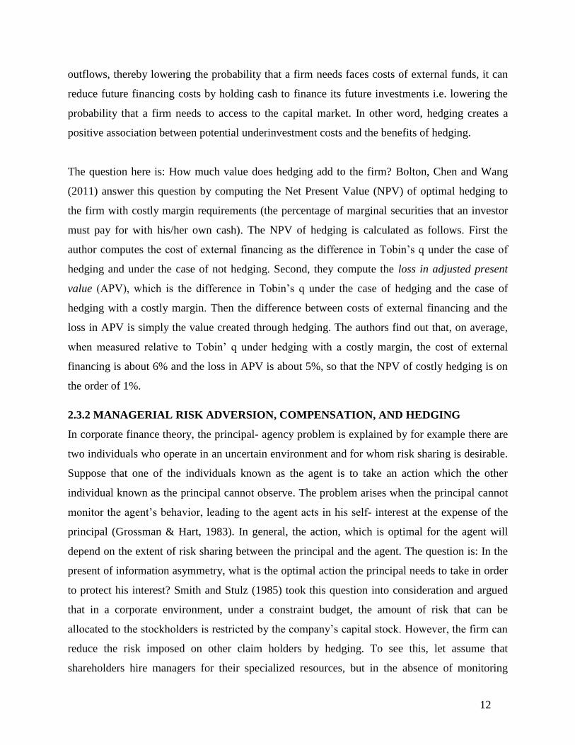
Financial distress costs consist of two forms: direct and indirect costs. Direct costs refer to a
situation when in the case of bankruptcy; firms need to pay fees for lawyers, expert witnesses
and administrative and accounting fees. While indirect costs relate to the situation when firms
lose valuable contact with customers, suppliers or skillful employees. To demonstrate how
hedging can minimize the risk of bankruptcy, we can demonstrate with an example (Aretz,
Bartram & Dufey, 2007): Suppose an extremely distressed firm has a 60 percent chance of being
unable to repay its fixed obligations. It has a debt with a face value equal to 250 and that the
direct bankruptcy costs are 20 in this case of bankruptcy. If in the future, the firm’s revenue falls
below 250 then the firm will go bankrupt. The expected bankruptcy cost therefore, is: 0,6* 20 =
12. Assume that the firm incurs indirect costs of financial distress, which equal 18. The total sum
of both indirect and direct costs in case of bankruptcy adds up to 30. If the firm hedges its future
cash flow to be more than 250 then the firm will not default.
Figure 2. Bankruptcy and financial distress (Aretz, Bartram & Dufey, 2007 pp.442)

15
Figure 1 above shows the distribution of cash flows of a firm, which is unable to pay off the debt
to its debt holders when the cash flow drops under FPO. As the probability of falling below this
point is positive, the firm may go bankrupt with a positive bankruptcy costs. If corporate risk
management ensures that firm’s future cash flow will be above FPO, firm value increases from
𝐸1(𝑉) to 𝐸2(𝑉).
So far, we have discussed the benefit of hedging to potential bankruptcy, but we still do not take
into consideration the size of hedging costs. One question remains if hedging still increases the
firm value if the costs of hedging are significant? Warner (1977) pointed out that in case if the
transaction costs of bankruptcy costs are a small fraction of large firms’ assets and they are less
likely the reason for firms to hedge. However, if the reduction on expected bankruptcy costs
exceeds the costs of hedging then large firms will likely to hedge. The same argument applies for
small firms as well; since the expected bankruptcy costs are a significant fraction of the small
firm’ assets, then the reduction in expected bankruptcy costs is greater for the small firms.
Therefore, they will be more likely to hedge.
Smith and Stulz (1985) explored the fact that hedging still give benefits to the firm give the fact
that the hedge decreases the present value of bankruptcy costs and increases the present value of
the tax shield of debt. To maximize the firm value, one thing managers can do is choosing the
hedging alternative that has lower cost.
2.3.4 TAX BENEFITS AND HEDGING POLICIES
The structure of the tax code can make it advantageous for firm to take positions in futures,
forward, or options markets. To analyze the effect of hedging on the present value of the firm’s
after- tax cash flow, I will use the demonstration taken from (Smith & Stulz, 1985). We can
assume that there are s states of the world, with 𝑉𝑖 defined as the pre- tax value of the firm in
state of the world i. States of the world are numbered so that 𝑉𝑖 < 𝑉𝑗 if i < j. Let 𝑃𝑖 be the price
today of one dollar to be delivered in state of the world i and T (𝑉𝑖) be the tax rate if the before-
tax value of the firm is 𝑉𝑖. In the absence of leverage, the value of the firm after taxes, V (0), is
given by:
(1) V (0) = ∑ 𝑃𝑖 (𝑉𝑖 − T (𝑉𝑖)𝑉𝑖)𝑆𝑖=1

16
Hedging can increase the value of the firm if there two states in the world, j and k, such that T
(𝑉𝑖) < T (𝑉𝑘). To demonstrate it, suppose that the firm holds a hedge portfolio such that 𝑉𝑗 + 𝐻𝑗 =
𝑉𝑘 + 𝐻𝑘, and that the hedge portfolio is self- financing in the sense that 𝑃𝑗 𝐻𝑗 + 𝑃𝑘 𝐻𝑘 = 0. Let
𝑉𝐻(0) be the value of the hedged firm. Then we have:
(2) 𝑉𝐻(0) – V (0) = 𝑃𝑗 (T (𝑉𝑗)𝑉𝑗 − T (𝑉𝑗 + 𝐻𝑗) (𝑉𝑗 + 𝐻𝑗))
+ 𝑃𝑘 (T (𝑉𝑘)𝑉𝑘 − T (𝑉𝑘 + 𝐻𝑘) (𝑉𝑘 + 𝐻𝑘)) > 0
The inequality implies that (2) is a concave function. Therefore, costless hedging increases the
value of the firm.
Figure 3: Tax and Hedging policies (Aretz, Bartram & Dufey, 2007 pp.443)
Figure 2 above show illustrated the fact if the firm tax schedule is a convexity, and then the firm
faces a higher expected tax burden in the case of high volatile pre- tax income than in case of
stable income. Therefore, the value of hedging will increase firm value compare with when the
tax schedule is linear.
However, there are contradict about corporate tax shields can induce value maximizing
corporation to hedge their operating cash flows. Kale and Noe (1990) point out that corporate

17
debt tax shields can prevent firms from hedging. The intuition behind this statement is that value-
maximizing firm will set its hedging policy with the objective of minimizing the sum of financial
distress costs. If the corporate tax code exhibits convexity and personal tax rates are linear, then
the act of hedging can actually lower the value of the firm. As mentioned earlier in the Debt and
Hedging policies part, firm will choose to hedge if the benefit of hedging exceeds the financial
distress costs then firm will be better off to hedge. Nonetheless, if the effective corporate tax rate
is low and the costs of bankruptcy are low, and then the effect of hedging will be to lower the
value of the firm.
2.4 SUMMARY
There are two contradicting theories about whether firms should hedge or not. According to the
neoclassical investment theories (Modigliani& Miller, 1958; Hayashi, 1982), in an efficient
market (assuming CAPM hold) hedging is fruitless since investors with access to perfect
information can manage to reduce the risk in their portfolios by themselves. In other word,
hedging creates no value to the firm.
Nonetheless, in the presence of realistic capital market imperfections, i.e. agency costs, costs of
external financing, direct and indirect bankruptcy costs, as well as taxes, corporate hedging will
enhance the shareholder value. The theories about why firms choose to hedge can be divided into
two categories: (1) Shareholder value maximization theory and (2) The structure of financial
structure and tax code. The shareholder value maximization theory highlights the fact that when
the compensation ties to the manager’s performance in term of the stock price movements i.e. if
the future’s stock price can affect management’s compensation, then the potential decline in
stock price will intensify the risk aversion if undiversified managers. Hence, a risk adverse
manager will stay away from risky projects, leading to underinvestment problem. One solution to
this underinvestment problem is to hedge against the fluctuation of the stock price movement
(Smith & Stulz, 1985; Froot, Scharfstein& Stein, 1993; Aretz, Bartram& Dufey, 2007).
Regarding the financial structure and tax code of the company, the motivations behind firm’s
decision to hedge are to (1) minimize the risk of bankruptcy and (2) reduce the corporate tax
burden if the firm tax schedule is a convexity, then the firm faces a higher expected tax burden in
the case of high volatile pre- tax income than in case of stable income. Therefore, the value of

18
hedging will increase firm value compare with when the tax schedule is linear (Smith & Stulz,
1985; Aretz, Bartram& Dufey, 2007).

19
3. METHODOLOGY
This chapter will describe the methodology used when developing this thesis and how the data
was collected, followed by different diagnostics tests. In the end of this chapter, I present the
OLS equation for estimating the firm value.
3.1 RESEARCH APPROACH AND STRATEGY
The research approach is used in this study has a quantitative nature, which is “explaining
phenomena by collecting numerical data that are analyzed using mathematically based methods”
(Aliaga & Gunderson, 2000). In order to find out if hedging can affect firm value or not, all the
data need to be tested by using Eviews- a software program for time- series oriented econometric
analysis.
Two empirical studies are used extensively in this thesis as benchmarks. The first one is
Allayannis and Weston (2001) and the second one is Jankengard (2015), both studies provide
great analysis and data about the subject. Nonetheless, I pay most attention to Jankengard’s study
by following reasons:
The methodology in which the author used is very well described and easy to replicate.
The author was one of few researchers that study Swedish firms’ derivatives usage at a
very deep level and his research provides great guidance to my own study.
3.2 DATA COLLECTION
The data used consisted of 90 Swedish firms listed on the Stockholm Stock Exchange, having the
total assets exceeds at least 1 billion Euros. Initially 353 firms were extracted from DataStream,
thereafter I excluded all the financial service firms, because most of them are also market makers
in Foreign Currencies derivatives, hence their motivations for using derivatives may be different
from the motivations of nonfinancial firms. I also excluded public organizations because they are
heavily regulated. The next step is to delete all the firms that don’t have complete data. This is an
easy task since most of the data was extracted from the Data Stream. After the selection, I was
left with 90 firms.
The choice of sample selection is very critical to the accuracy of results. Firstly, the sample is
limited to the Swedish large and mid-cap firms in different industries with different growth rates.
Comparison of the value may be affected by other variables not included in the analysis.

20
Secondly, I am aware that firms in different industries with different growth rates can make the
comparison bias since the firm value can be affected by other variables not include in the
analysis.
3.3 RESEARCH PROCEDURES
The purpose of this study is to document the impact of hedging on firm value. However, there
are other variables that may affect the firm value as well, such as: profitability, leverage,
dividend, industrial diversification, firm size, CAPEX (Allayannis & Weston, 2001; Jankengard,
2015). To take those variables into account, a multivariate setting will be used to test the
hypothesis that hedgers have higher values than non-hedgers.
Firm value: To estimate the firm value, I use Tobin’s Q. Tobin’s Q is defined as the ratio of the
market value of the firm to replacement cost of assets, evaluated at the end of the fiscal year. I
compute Tobin’s Q for a total of 540 firm- year observations (Total 90 firms * 6 years).
According to Allayannis and Weston (2001), one more advantage of using Tobin’s Q is that it
makes the comparisons across firms easier than comparisons based on stock returns or
accounting measures where a risk adjustment or normalization is required.
Hedging: The information about whether the selected firms hedge or not can be collected manual
from the annual reports. I go through the reports for each firm and take note about their risk
management. In most cases, this information was easy to obtain since most companies disclosure
about their risk management program and also are clearly about why they choose to hedge. They
declare that the purpose of hedging is not for speculative activities but rather to minimize the
volatility of future cash flows and exposure to currency exchange rates. I use derivatives as a
dummy variable that take the value one if the firm hedge and zero otherwise. Using dummy
variable is appropriate for my regression analysis because it is hard to measure the size of
hedging costs since most companies only disclosure the fact that they are involving in risk
management program but do not articulate the magnitude of hedging costs in their financial
reports.
Similarly to Jankengard (2015), besides the test variable hedging, I also choose other control
variables that can affect the firm value such as: Dividend, firm size, profitability, leverage,
diversification and CAPEX. I also want to include the variable foreign sales ratio as a control

21
variable. However, due to the severe lack of relevant data, this variable needs to be excluded
from the analysis.
Dividend: is a dummy variable and takes the value of one if the firms pay dividends and zero
otherwise. The reason to why I take dividend payment into my study is there are previous
research providing the evidence that dividend payout announcement can impact firm value due
to higher dividend payout rate, the higher is the tax cost of the dividend, which dampens the
increase in firm value (Kane, Lee & Marcus, 1984; Murdoch, 1992). Nonetheless, there is also
evidence that supports the hypothesis that dividend payout enhances firm value since it signals to
the market that the firm in question is in a good financial shape, and in turn the investors reward
the firm with higher valuation (Jin & Jorison, 2006).
Firm size: There is ambiguous evidence for U.S firms that the size of the firm leads to higher
accounting profitability (Allayannis & Weston, 2001), due to the existence of large fixed start-
up costs of hedging, the firm size is determined by taking the logarithm of Total Assets.
Profitability: A profitable firm is likely to trade at a premium relative to a less profitable one.
This variable is equal to Net Income/ Total asset (Jankengard, 2015).
Leverage: A firm’s capital structure can affect its value. In Modigliani and Miller (1958)
demonstrated that in a frictionless world, financial leverage is unrelated to firm value. However,
in a world with tax- deductible interest payments, firm value and capital structure are positively
related (Antwi, Mills & Zhao, 2012). A firm’s capital structure may affect its value. To control
for leverage, I take Total Debt/Total Assets.
Industrial Diversification: This data was collected manually; I go through annual reports of all
firms and take note if the companies operate in two or more product segments. This control
variable is a dummy variable and takes the value one of the companies have more than two
segments and zero otherwise. The reason, I want to include this variable in my regression
analysis is that there are several theoretical suggest that industrial diversification increases value
(Williamson, 1970; Jensen, 1986).

22
CAPEX: is defined as additions to Fixed Assets/Total Sales.
Table 1: Summary of variables and data sources
Definition
Source
Tobin' Q The log of (total book Datastream
value of assets less book
value of equity plus market
value of equity) / Total assets
Hedging A dummy variable that has value 1 Annual reports
if the firm hedges and 0 otherwise
Leverage Total debt/ Total Assets Datastream-
CAPEX Additional fixed assets Datastream
Profitability Net income/ Total assets Datastream
Firm size Logarithm of total assets Datastream
Dividend A dummy variable that takes value 1 Datastream
if firm pays dividend and 0 otherwise
Diversified A dummy variable that takes value 1 if the Annual reports
firm has more than 2 product segments and
0 otherwise
Since I have different companies and a six- year period, I organize the collected data into panel
data in order to use the software program Eviews. The advantages of panel method comparing to
other methods are those that a panel of data will embody information across both time and space.
Most importantly, a panel keeps the same individuals or objects and measures some quantity
about them over time (Brooks, 2008).

23
Table 2: Descriptive Statistics
Number Min Max Median Mean St. Dev
Tobin' Q 85 0,24 6,26 1,21 1,55 1,09
Hedging 60 1,00 1,00 0,77 0,42
Leverage 72 0,69 0,17 0,19 0,16
CAPEX 85 0,80 0,02 0,05 0,10
Profitability 85 -0,17 0,57 0,01 0,01 0,04
Firm size 85
3,30 8,56 6,46 6,58 0,95
Dividend 80 1,00 1,00 0,69 0,46
Diversified 85 1,00 0,00 0,32 0,47
The table above describes the descriptive statistic for all the control variables. Using the
descriptive statistic is a good way to spot possible problems with the data (outliners and so on)
and it also gives an idea about the distribution of the variables while interpreting the regression.
As we can see from the descriptive statistic table, the median of Tobin’s Q is 1, 21, which is
smaller than the mean Tobin’s Q (1, 55) indicates that the distribution of Tobin’s Q is skewed.
To control for the skewness, the natural log of Tobin’s Q will be used in the multivariate test so
that the distribution of Tobin’s Q will be more symmetric.
The equation for the regression is:
Log(Tobin’s Q) = c+ 𝛽1*capex + 𝛽2 *diver + 𝛽3*dividend + 𝛽4*hedge
+ 𝛽5*leverage + 𝛽6*profit +𝛽7*size
Since I used panel data for my study, the remained question is to choose Fixed or Random
effects? According to Brooks (2008, pp. 500) the random effects model is more appropriate
when the entities in the sample can be thought of as having been randomly selected from the
population, but a fixed effect model is more plausible when the entities in the sample effectively
constitute the entire population. Furthermore, the fixed effects model also allows cross- sectional
heterogeneity. In my data sample, there are 90 firms in different industries and it is unlikely to
assume that there is no heterogeneity. One more advantage of using fixed effects model is that all

24
the unobservable firm characteristics that may affect firm value can be controlled since each firm
is assigned a unique intercept (Hausman & Taylor, 1981).
In Eviews, I still perform both of the tests in order to find the most suitable one. (1) I select the
fixed effects on the cross section after that I run the Redundant Fixed Effect- Likelihood Ratio,
the P- value is 0,000 indicating that the effects are significant. (2) Select the random effect and
perform the Correlated Random Effects- Hausman test. In this test, I am testing the random
effects model against the fixed effects model. The null hypothesis in that case is that both tests
are consistent estimators and the random effects model is efficient. Under the alternative
hypothesis, only the fixed effect is consistent. Since the p- value is 0.000, I reject the null and,
therefore, the fixed effects model is to be preferred.
3.4 STATISTICAL DISTRIBUTIONS FOR DIAGNOTIC TESTS
In order to run an OLS regression with the highest accuracy as possible, I need at first run
various regression diagnostic tests that are based on the calculation of the test statistic.
For the classical OLS to work well, there are three basic assumptions that need to be satisfied in
order to have an unbiased OLS estimation.
(1) E(𝑢𝑡) = 0
(2) Var(𝑢𝑡)= 𝜎2
(3) Cov(𝑢𝑖, 𝑢𝑡) = 0
The first assumption (1) required that the average value of the errors is zero. However, when I
estimate OLS, a constant term is included in the regression equation so this assumption will not
be violated.
For the second assumption (2), it has been assumed so far that the variance of the errors is
constant. This is known as the assumption of homoscedasticity. If the errors do not have a
constant variance, they are said to be heteroscedastic. The consequence of not having a constant
variance is that estimation of OLS will be biased. In order to detect if there is some evidence of
heteroscedasticity, I run the Goldfeld Quandt test.

25
Assumption (3) requires that the covariance between the error terms over time is zero. In other
word, it is assumed that errors are uncorrelated with one another. Because the population
disturbances cannot be observed, so a test for this is necessary. I will use the Watson- Durbin test
for this purpose.
One more potential problem that may occur is the relationship between the dependent variable
and independent variables. For example, Froot et al. (1993) pointed out that the more valuable
the firm’s investment opportunities, the more attractive risk management becomes because
disruptions to the investment program are more costly, this lead to the endogeneity problem. To
test for this possibility, I will carry out the procedure recommend by Hausman, which involves
using the residuals with hedging as dependent and other variables such as: Firm’s size,
profitability, leverage, CAPEX, dividends, diversified as exogenous variables. However, since
fixed effects test allows for heterogeneity then Hausman test for endogeneity will not be
performed.
Detection of heteroscedasticity
The Goldfeld Quandt is based on splitting the total sample of length T into two sub- samples of
length 𝑇1and 𝑇2 . The regression model is estimated on each sub-sample and the two
residual variances are calculated as 𝑠12= �̂�1
´ �̂�1 / (𝑇1-k) and
𝑠22= �̂�2
´ �̂�2 / (𝑇2-k) respectively. The null hypothesis is that the variances of the disturbances are
equal, which can be written as 𝐻0: 𝜎12 = 𝜎2
2, against a two- sided alternative. If we reject the null
hypothesis then we can conclude that our model contain heteroscedasticity problem i.e. the
variances of the error terms are not constant.
Detecting autocorrelation
As mentioned earlier the Durbin- Watson (DW) is a useful test for detecting the first order
autocorrelation i.e. it tests only for a relationship between an error and its immediately previous
value. The test equation is:
𝑢𝑡= 𝜌𝑢𝑡−1+ 𝑣𝑡
Where 𝑣𝑡~ N (0, 𝜎𝑣2), the DW test statistic has as its null and alternative hypotheses are:

26
𝐻0: 𝜌= 0 and 𝐻1= 𝜌≠ 0
If 𝜌≠ 0, we can reject the null and conclude that there is evidence of a relationship between
residuals i.e. correlation.
After I run Goldfeld Quandt test for heteroscedasticity and Durbin-Watson for autocorrelation to
make sure that there are no errors in the collected data. The next step is to estimate an OLS
model for testing hedging premium based on the following equation:
Log(Tobin’s Q) = c+ 𝛽1*hedging + 𝛽2*leverage + 𝛽3*CAPEX + 𝛽4*profitability + 𝛽5*size +
𝛽6*dividend +𝛽7*diversifie
3.5 LIMITATION
The first limitation in methodology is due to the time constraint and difficulties in gathering
complete data set, I will exclude some variables that can affect firm value such as:
NETPOSITION and FOREIGN, though two variables may have significant impact on firm
value. The variable NET Position is defined as the sum of absolute of the net position in each
currency (expressed in units of home currency scaled by total assets. FOREIGN is the ratio of
Foreign Sales to Total Sales. Previous studies showed that these variables impact firm value
since they connect directly to the currency risks (Jankengard, 2015).
The second limitation is the univariate tests will be excluded from this study since even if
univariate tests show hedging variable significant when the multivariate tests do not then a
conclusion cannot be drawn based on univariate tests. Hence, because of the time shortage, only
multivariate tests are performed.

27
4. RESULTS AND ANALYSIS
This chapter will present the results of the statistical tests and the OLS regression analysis. Since
there may be another alternative explanation for the ordinary OLS, I also consider the
robustness of the result and the re-estimation of the model is also presented at the end of the
chapter.
4.1 EMPIRICAL FINDINGS
4.1.1 STATISTICAL TEST
For Goldfeld Quandt test: The t- statistic is 2, 72 and the P- value is 0,000, we can conclude that
there is no evidence for the presence of heteroscedasticity. For Durbin- Watson (DW) Test: the
Test- statistic is 1, 46 indicating that there is no autocorrelation between the residuals since
theoretically speaking, if DW is close to 2, we can assume that there is no evidence of
autocorrelation (Brooks, 2008). The results of the diagnostic tests signal that I can go ahead to
run OLS regression analysis.
4.1.2 HEDGING AND FIRM VALUE USING MULTIVARIATE TEST
The explanatory variables for the equilibrium test regression are CAPEX, diver, dividend, hedge,
leverage, profit and size. The dependent variable is the log of Tobin’s Q. The null hypothesis for
fixed effects is jointly zero (𝐻0 : ƞ𝑖 = 0). Since the P- value of fixed effects is 0.000 so I
reject 𝐻0 , meaning that the firm value is affected differently by the same variables
(heterogeneity).
The result of the regression analysis shows that out of seven control variables, only size and
profit are statistically significant at 5% level, telling us that size and profit affect the firm value
positively. If firm increases its profit then the value of the firm will also be rewarded with higher
value. The variable size is significant at 5% level indicating that larger firms have a stronger
tendency to have higher value than smaller firms.

28
Table 3: An OLS model of firm value
Note: t- ratios in parentheses, * and ** denote significance at the 1% and 5% levels respectively
4.1.3 ROBUSTNESS
To check the robustness of the results, the model is re-estimated using different subsamples. This
method is used to address outliner concern. One way to do this is using the Descriptive Statistics
to find out if there are many too large numbers that deviate significantly from the mean value,
then I will delete them and then re-estimate the model. There are also other concerns that need to
be taken into account. In my data sample, some of the companies such as H& M and Fingerprint
Cards AB don’t have any debts at all, so those companies should not be included in the
estimation since the t- stat for leverage may be affected. Furthermore, since the time period for
the data is from 2005- 2010, due to the severe down turn in the economy because of the financial
crisis; some of the companies in the data sample do not have dividend payments continuously.
Some of them cut the dividends between years 2008 and 2009. Therefore, I also exclude those
companies in order to avoid robustness in the dividend variable.
C 0,47
(0,22)
CAPEX 0,05
(1,51)
DIVER – 0,06
(2,14)
DIVIDEND 0,04
(0,116)
HEDGE 0,04
(0,93)
LEVERAGE – 0,54
(3,73)
PROFIT 0,29
(2,12)**
SIZE 0,04
(2,27)**

29
Below is the re- estimated OLS model:
Table 4: Robustness check for the impact of hedging on firm value
Note: t- ratios in parentheses, *, ** and *** denote significance at the 1%, 5% and 10% levels
respectively.
After re-estimate the model I get a slightly different result. The coefficients for the seven control
variables have different signs, suggesting a different effect on the dependent variable. For
instance: the control variables for diversified (diver) and leverage have the negative sign (though
diver is not statistically significant) meanwhile leverage is statistically significant at the 5%
level.
One more difference that can be observed here is that the variable dividend is significant at 10 %
level.
The control variables CAPEX, hedge and diver are not statically significant.
C 0,6
(1,31)
CAPEX 0,45
(1,59)
DIVER – 0,04
(2,07)
DIVIDEND 0,013
(0,42)***
HEDGE 0,58
6,9
LEVERAGE – 0,4
(1,9)**
PROFIT 1,79
(2,56)**
SIZE 0,36
(2,19)**

30
4.2 ANALYSIS OF THE FINDINGS
The finding indicates that there is no relationship exists between hedging and firm value since
the variable hedging is insignificant, although the coefficient of this test variable is positive. This
finding is in contrast to some studies in the literature (Allayannis & Weston, 2001; Jankengard,
2015). The time panel, which this study cover is from 2005 to 2010 and intuitively one might
expect that the risk management program would be considered more valuable during the crisis.
As a well known fact that, since Sweden is an export dependency country and the fact that the
macro condition is quite favorable for Sweden in term of a weakened Krona against major
currencies such as USD and EUR. For instance, in 2009 the averages for these exchange rates
versus SEK were 11% and 13% above their average for 2006- 2008, respectively (Jankengard,
2015). Previous research (Smith & Stulz, 1985; Bartram, 2000; Aretz, Bartram & Dufey, 2007)
supports the value maximization theory, in which managers engage in risk management in order
to secure the future cash flows, especially when the managers’ compensation is tied to the
performance of the firms. As a consequence of the financial crisis, we should not rule out the
probability that the profits Swedish firms gained from net- export due to a weakened Krona can
impair the effect of derivatives usage (the coefficient of test variable hedging is positive, we can
assume that hedging impacts firm value positively but nonetheless, we can not prove a
significant relationship). This theory is also consistent with the findings of Geczy, Minton and
Schrand (1997), suggesting that the potential benefits of using currency derivatives depend on
the firm’s exposure to foreign exchange- rate risk. They find that firm characteristics related to
these costs and benefits are related to how firm forecast its future cash flows. If the forecast is
accuracy, indicating higher profitability then firm has less incentive to hedge.
The variable leverage is significant at 5% level, and the negative sign of variable indicates that if
a firm has less debt (leverage) its value will increase more. This result is expected since an
increase in debts leads to higher distress costs (Aretz, Bartram & Dufey, 2007). Previous studies
have shown that highly leveraged firm lose substantial market share to more conservatively
financial competitors in industry down turns. A similar decline also takes place in the market
value of equity (Opler & Titman, 1994; Ogden, Jen & O’Connor, 2003). Smith and Stulz (1985)

31
also pointed that a firm’s high level of debt is one of the main reasons mangers choose to hedge
if corporate risk management ensures that firm’s future cash flow will be secured.
Dividend variable is statistically significant at 10% level, and it tells us that whether the firm
pays dividend or not will affect its value. This result is consistent with what is found in Jin and
Jorison (2006), that dividend payouts may be viewed as a positive signal from management since
it signals to the market that the firm in question is in a good financial shape, and in turn the
investors reward the firm with higher valuation.
Size is statistically significant at 5% level, indicating that larger firms tend to have higher value.
This result is consistent with what is found in Allayannis and Weston (2001), which states that
the size of the firm leads to higher accounting profitability. However, the positive correlation
between size and firm value is inconsistent with that of Bodnar, Tang and Wientrop (1999),
according to the findings of this study, bigger firms are, the more multinational they are and
when they do business in more than country, efficient and effectiveness are likely to become low
due to the lack of corporate governance. This problem has been mentioned many times in
corporate finance theory as principal and agency problem (Grossman & Hart, 1983). This is to be
said, the shareholders’ value maximization goal may differ from the managers’ objectives
leading to less firm value.
The variable profit is significant at 5 %, indicates a positive correlation between profit and firm
value. The influence of profitability on firm value has long been discussed in the literature
(Modigliani & Miller, 1958; Myer, 1984). An increased firm value due to a higher profitability is
related to the pecking order theory (Myer, 1984) which states that when a firm has a need for
capital to invest in some attractive projects, the optimal choice for firm is to fund the project with
its internal fund (cash) since external financing (issuing debt or equity) can be costly due to
information asymmetry. Therefore, higher profitability makes firm less vulnerable for external
funds. Haugen and Baker (1996); Yang et al. (2010); Chen and Chen (2011) also proved that the
greater is the firm’s profit, the more distributable earnings there are for shareholders, and hence
the expected firm value will be higher.

32
5. CONCLUSION
This project research studies the impact of hedging on firm value using a sample of 90 Swedish
companies listed on the Stockholm Stock Exchange from 2005 through 2010. I examine whether
the act of hedging is rewarded by investors with a higher market valuation.
Using Tobin’s Q as an approximation for firm market value and hedging as a control variable, I
found insignificant evidence that the usage of hedging impacts firm value positively. However, I
found evidence about other factors such as: dividend, leverage, firm size and profitability affect
the firm value differently. Leverage has a negative impact (the coefficient is negative), indicates
that the higher the debt level in the firm’ capital structure the less valuable firm is, while other
variables such as: firm size, profitability, and dividend affect firm value positively.
Recently, the relationship between hedging and firm value has been studied extensively, and this
research report is supposedly contribute to a better understanding of the risk management
program. There an important implication from these findings that is the link between hedging
and firm value does not support the notion that hedging increase firm value. Consequently,
managers need to evaluate and consider whether to participate in the corporate risk management
program. However, due to the mixed result of whether hedging can impact firm value positively,
more research in this area is necessary before we can draw a firm conclusion about the impact of
hedging on firm value.

33
6. REFERENCES
Ahmed, H., Azevedo, A. & Guney, Y. (2010) “The effect of Hedging on Firm Value and Performance:
Evidence from the Nonfinancial UK Firms”, Working Paper, Hull University Business School
Aliaga, M. & Gunderson, B. (2000) “Interactive Statistics”, Saddle River
Allayannis, G. & Weston, P. J. (2001) “The Use of Foreign Currency Derivatives and Firm Market
Value”, The Review of Financial Studies, Vol.14 No.1 243- 276
Antwi, S., Mills, E. & Zhao, X. (2012) “Capital Structure and Firm Value: Empirical Evidence from
Ghana”, International Journal of Business and Social Science, Vol. 3, No. 22
Aretz, Bartram & Dufey. (2007) “Why hedge? Rationales for corporate hedging and value
implications”, The Journal of Risk Finance, Vol.8 No.5 pp. 434-449
Asquith, P. & David, M. (1986) “Equity issues and offering dilution”, Journal of Financial Economics
15, 61–89
Bartram, S. M. (2000) “Corporate risk management as a lever for shareholder value creation”,
Financial Markets, Institutions and Instrument, Vol.9 No.5 pp. 279- 324
Bodnar, G.M, Tang, C. & Weintrop, J. (1999) “Both Side of Corporate Diversification: The
Value Impact of Geographic and Industrial Diversification”, Working Paper, John Hopkin
University
Bolton, M., Chen, H. & Wang, N. (2001) “A Unified Theory of Tobin’s q, Corporate Investment,
Financing, and Risk Management”, The Journal of Finance Vol. LXVI, No 5
Brooks, C. (2008) “Introductory Econometrics for Finance”, Cambridge University Press,
Cambridge, UK
Chen, J. & Chen, Y. (2011) “The Influence of Profitability on Firm Value with Capital Structure
as the mediator and Firm Size and Industry as Moderators”, Investment Management and
Financial Innovations, Vol. 8, No. 3

34
Dufey, G. & Srinivasulu, S.L. (1983) “The case for corporate management of foreign exchange
risk”, Financial Management, Vol. 12 No. 4, pp. 54-62.
Fama, F.E. & French, R.K. (2004) “The Capital Asset Pricing Model: Theory and Evidence”,
Journal of Economic Perspective Vol. 18, no. 13
Fauver, L. & Naranjo, A. (2010) “Derivative usage and firm value: The influence of agency
costs and monitoring problems”, Journal of Corporate Finance, Vol. 16, pp. 719- 735
Gay, D. G. & Nam, J. (1998) “The Underinvestment Problem and Corporate Derivatives Use”,
Financial Management, Vol. 27, No. 4, pp. 53- 69
Geczy, C., Minton, B. & Schrand, C. (1995) “Why Firms Use Derivatives Distinguishing among
Existing Theories”, working paper, Wharton Business School, University of Pennsylvania
Grossman, S. & Hart, O. (1983) “An Analysis of the Principal- Agent Problem”, Journal of The
Econometric Society, Vol. 51, No. 1 pp.7-45
Guay, W. & Kothari, S. P. (2002) “How much do Firms Hedge with Derivatives?”
Hagelin, N. (2003) “Why firms hedge with currency derivatives: An examination of transaction
and translation exposure”, Applied Financial Economics, Vol. 13 pp. 55-69
Haugen, R. A. & Baker, N. L. (1996) “Commonality in the determinants of expected stock
returns”, Journal of Financial Economics, Vol. 41, pp. 401- 439
Haushalter, D. (2000) “Financing Policy, Basic Risk, and Corporate Hedging: Evidence from Oil
and Gas Producers”, Journal of Finance¸ Vol. LV, No.1
Hausman, J. & Taylor, W. (1981) “Panel Data and Unobservable Individual Effects”,
Econometrica, 49, pp.1377- 1398
Hayashi, F. (1982) “Tobin’s Marginal q and Average q: A Neoclassical Interpretation”,
Econometrica, Vol.50, No.1, pp. 213-224
Jankengård, H. (2015) “Does Centralisation of FX Derivative Usage Impact Firm Value?”,

35
European Financial Management Vol.21, No.2 pp. 309-332
Jensen, M. (1896) “Agency Costs of Free Cash Flow, Corporate Finance and Takeovers”,
American Economic review, Vol. 76 pp. 323-329
Jin, Y. & Jorion, P. (2006) “Firm Value and Hedging: Evidence from U.S Oil and Gas
Producers”, The Journal of Finance, Vol. LXI
Kale, J.R. & Noe, T.H. (1990) “Corporate hedging under personal and corporate taxation”,
Managerial and Decision Economics, Vol.11, No.3, pp.199- 205
Kane, A, Lee, Y. & Marcus, A. (1984) “Earnings and Dividend Announcements: Is there a
Corroboration Effect?”, The Journal of Finance, Vol. 39, No.4 pp. 1091-1099
Modigliani, F. & Miller, M. (1958) “The cost of Capital, Corporation Finance and The Theory of
Investment”, The American Economic Review, Vol. XLVIII, No. 3
Murdoch, A. (1992) “Dividends and earnings: Their effect on firm value”, working paper,
University of Washington
Myers, S. C. (1984) “The Capital Structure Puzzle”, Journal of Finance, Vol. 39, pp. 575- 592
Ogden, J.P., Jen, F.C. & O’Connor, P. F. (2003) “Advanced Corporate Finance: Policies and
Strategies”, Prentice Hall
Opler, T. & Titman, S. (1994) “Financial Distress and Corporate Performance”, The Journal of
Finance, Vol. 49, No. 3 pp. 1015- 104
Rothschild, M. (1985) “Asset Pricing Theories”, Technical Working Paper, No.44
Scholes, M. (1972) “The marker for securities: Substitution versus price and the effects of
information of share prices”, Journal of Business, Vol. 45 pp.179-211
Smith, W.C., & Stulz (1985) “The Determinants of Firms’ Hedging Policies”, Journal of
Financial and Quantitative Analysis, Vol.20, No.4

36
Stulz, R. (1996) “Rethinking Risk Management”, Journal of Applied Corporate Finance, Vol. 9,
No.3 pp. 8-25
Warner, J. (1977) “Bankruptcy costs: Some Evidence”, Journal of Finance, Vol.32 pp.337- 348
Williamson, O. (1970) “Corporate Control and Business Behavior: An Inquiry into the Effects of
Organizational Form on Enterprise Behavior”, Prentice Hall, Englewood Cliffs, N.J.
Yang, C.C., Lee, C.F., Gu, Y.X. & Lee, Y. W., (2010) “Co-determination of Capital structure
and Stock Returns- A LISREL approach: An Empirical Test of Taiwan Stock Market”, The
Quarterly Review Of Economics and Finance, Vol. 50, pp. 222- 233
Website: www.ourcommunity.com.au (n.d)

37
7. APPENDIX
1, Heteroskedasticity Test: Breusch-Pagan-Godfrey
F-statistic 2.722032 Prob. F(7,424) 0.0000
Obs*R-squared 31.24230 Prob. Chi-Square(7) 0.0001
Scaled explained SS 33.13285 Prob. Chi-Square(7) 0.0000
Test Equation:
Dependent Variable: RESID^2
Method: Least Squares
Date: 05/07/15 Time: 17:39
Sample: 1 432
Included observations: 432
Variable Coefficient Std. Error t-Statistic Prob.
C -0.001152 0.048089 -0.023950 0.9809
CAPEX -0.006146 0.014176 -0.433550 0.6648
DIVER 0.015551 0.011865 1.310685 0.1907
DIVIDEND 0.022842 0.012749 1.791653 0.0739
HEDGE 0.023055 0.015709 1.467665 0.1429
LEVERAGE -0.162921 0.037059 -4.396251 0.0000
PROFIT -0.312874 0.123396 -2.535526 0.0116
SIZE 0.010867 0.006537 1.662204 0.0972
R-squared 0.072320 Mean dependent var 0.078686
Adjusted R-squared 0.057005 S.D. dependent var 0.116893
S.E. of regression 0.113512 Akaike info criterion -1.495463
Sum squared resid 5.463274 Schwarz criterion -1.420122
Log likelihood 331.0201 Hannan-Quinn criter. -1.465719
F-statistic 4.722032 Durbin-Watson stat 1.459300
Prob(F-statistic) 0.000040
2, Fixed effects
Redundant Fixed Effects Tests
Equation: Untitled

38
Test period fixed effects
Effects Test Statistic d.f. Prob.
Period F 12.498058 (5,497) 0.0000
Period Chi-square 60.402435 5 0.0000
Period fixed effects test equation:
Dependent Variable: TOBQ_LOG
Method: Panel Least Squares
Date: 05/07/15 Time: 15:43
Sample: 2005 2010
Periods included: 6
Cross-sections included: 90
Total panel (balanced) observations: 540
Variable Coefficient Std. Error t-Statistic Prob.
C 0.471898 0.094883 0.215400 0.0003
HEDGE 0.039482 0.032605 0.930910 0.2265
SIZE 0.036493 0.013542 2.274756 0.0043
PROFIT 0.293954 0.309939 2.121648 0.0407
LEVERAGE -0.537268 0.084558 3.725165 0.0000
CAPEX 0.046357 0.035421 1.511065 0.1122
DIVIDEND 0.042698 0.029954 0.115906 0.6718
DIVER -0.056292 0.027103 2.136967 0.5383
Redundant Fixed Effects Tests
Equation: Untitled
Test period fixed effects
Effects Test Statistic d.f. Prob.
Period F 12.498058 (5,497) 0.0000
Period Chi-square 60.402435 5 0.0000

39
3, Re- estimated fixed effects
Period fixed effects test equation:
Dependent Variable: TOBQ_LOG
Method: Panel Least Squares
Date: 05/09/15 Time: 18:13
Sample: 2005 2010
Periods included: 6
Cross-sections included: 80
Total panel (balanced) observations: 480
Variable Coefficient Std. Error t-Statistic Prob.
C 0.561898 0.094883 1.315400 0.0043
HEDGE 0.579482 0.032605 6.910910 0.7512
SIZE 0.360493 0.013542 2.194756 0.0073
PROFIT 1.793954 0.309939 2.561648 0.0107
LEVERAGE -0.387268 0.084558 1.945165 0.0000
CAPEX 0.456357 0.035421 1.591065 0.1132
DIVIDEND 0.012698 0.029954 0.423906 0.0718
DIVER -0.036292 0.027103 2.076967 0.1383
4, Random effects
Cross-section random effects test equation:
Dependent Variable: TOBQ_LOG
Method: Panel Least Squares
Date: 05/07/15 Time: 15:51
Sample: 2005 2010
Periods included: 6
Cross-sections included: 90
Total panel (balanced) observations: 540
WARNING: estimated coefficient covariance matrix is of reduced rank
Variable Coefficient Std. Error t-Statistic Prob.
C 1.951119 0.386389 5.049617 0.0000
HEDGE NA NA NA NA

40
SIZE -0.261930 0.058469 -4.479830 0.0000
PROFIT -0.046639 0.304752 -0.153040 0.8784
LEVERAGE -0.336977 0.116686 -2.887895 0.0041
CAPEX 0.034943 0.026230 1.332174 0.1835
DIVIDEND -0.052817 0.027932 -1.890869 0.0593
DIVER NA NA NA NA