Does Corruption Affect Health and Education - United …unpan1.un.org/intradoc/groups/public/documents/... · Does Corruption Affect Health and Education Outcomes in the Philippines?

Does Corruption Affect Health and Education Outcomes in the Philippines?

Omar Azfar *Institutional Reform and Informal SectorUniversity of Maryland at College Park

College Park, MD 20742

Tugrul GurgurDepartment of Economics

University of Maryland at College ParkCollege Park, MD 20742

We examine the effect of corruption on health and education outcomes in the Philippines. Wefind that corruption reduces the immunization rates, delays the vaccination of newborns,discourages the use of public health clinics, reduces satisfaction of households with public healthservices, and increases waiting time at health clinics. Corruption also has a negative effect oneducation outcomes: it reduces test scores, lowers national ranking of schools, raises variation oftest scores across schools and reduces satisfaction ratings. We also find that corruption affectspublic services in rural areas in different ways than urban areas, and that corruption harms thepoor more than the wealthy.

JEL Classifications: H4, I1, I2.Key words: corruption, decentralization, health care, education, service delivery.

* [email protected]. The research underlying this paper was supported by a grant from the World Bank,financed by the Netherlands Trust Fund. We are extremely grateful to Tony Lanyi for his management of thisproject, to Satu Kahkonen for survey design and implementation (assisted by the staff at Social Weather Stations),and to Diana Rutherford for excellent project support. We thank Shanta Devarajan, Malika Krishnamurty, JennieLitvack and Ritva Reinika at the World Bank for their support. We are also grateful for comments on an earlierdraft of this paper from those already mentioned, as well as from Roger Betancourt, and Peter Murrell and theattendees of the 2001 NEUDC conference. All errors are our own.

1

I. Introduction

There are several mechanisms by which corruption might undermine service delivery.

Corruption can increase the cost to consumers if a bribe is demanded in addition to the official

payment, which reduces demand for services and therefore may worsen health and education

outcomes. If however corruption takes the form of the official pocketing the payment intended

for the government, this reduces government resources allocated to service delivery, which

would also worsen outcomes. As noted by Pritchett (1996) the relationship between public

spending and outcomes is usually ambiguous in many countries, and this ambiguity may be a

reflection of differences in the efficacy of spending due to corruption. A number of past studies

have looked at the effect of corruption on public sector performance in health, education,

infrastructure, etc. (Gray-Molina et al. (1999), Gupta et al. (2002), Reinikka and Svensson

(2001), Rajkumar and Swaroop (2002)). In this paper we supplement these results and examine

the effects of corruption at the local level in the Philippines on health and education services.

This approach has the advantage that it keeps fixed a large number of variables that vary across

countries and cause omitted variable problems and other econometric problems in cross sectional

regressions.

Five years after the democratic revolution in the Philippines, the Local Governments Act

of 1991 devolved both political authority and administrative control of many health services and

other subjects to the provincial and municipal level. Much of the corruption in the Philippines

does appear to be at the local level: of the 336 corruption cases current in mid-2000, 49% were

against municipal mayors- the level of government, which is our focus in this study (Batalla

2000). Many observers have stated that corruption is the root cause of continued poverty in the

2

Philippines (World Bank (2000)). All this makes our study of local level corruption and service

delivery in the Philippines highly relevant in a country specific context.

In addition studies such as this one might have global relevance in terms of the

increasingly important question of the effect of corruption on service delivery. Our results

resonate with cross-country results (e.g., Gupta et al. (2002)), which find a negative correlation

between corruption and health outcomes. However, we acknowledge the difficulty of

generalizing from cross-country results and one possibly unrepresentative country, and would

prefer to replicate this study in other countries with a large number of local governments before

making global prescriptions.

This paper is structured as follows. We begin by describing the data. In particular we

examine in detail the quality of the data on corruption and are reassured by a number of

correlations across samples. The corruption perceptions of households, municipal administrators

and municipal health officers are all correlated with each other and the corruption perceptions of

households are highly correlated with the corruption perceptions of other households in their

municipality.

Emboldened by these findings, we begin to examine the consequences of corruption.

Here we use several different outcome measures from different sources. We use households’

reports of waiting time, their satisfaction with government health services, access to public

health clinics, immunization rate of children, and delay between the birth of a child and his/her

immunization. In each case we find the expected negative and significant effect of corruption on

performance. Our results for education are similar. We find a significant negative effect on test

scores, national ranking of schools, variation of test scores within schools, and household

assessments of satisfaction with public education. Our empirical analysis also highlights the

3

disproportionate burden of corruption on the poor. The perverse effect of corruption on health

and education outcomes is also more serious in rural areas as compared to urban areas.

We provide information about the experience of Philippines with decentralization

reforms in the next section. The data and the econometric models are described in sections 3 and

4, respectively. We analyze the consequences of corruption in section 5. The robustness of our

results is discussed in Section 6. A conclusion follows.

II. Country Background

The Philippines is a country of 70 million people who live upon thousands of islands that

lie between the Pacific Ocean and the South China Sea1. The larger of these islands have vast

expanses of mountains and jungles that physically separate large populations. The sheer

geography of the Philippines necessitated some form of decentralized or at least deconcentrated

governance for centuries, but this was not always combined with devolution of political

authority.

Decentralization in the Philippines was mandated by the new democratic constitution of

1987. The Local Government Code (LGC) enacted in 1991 significantly increased the

responsibilities and resources of sub-national governments: 77 provinces, 72 cities, 1526

municipalities and over 40,000 barangays or neighborhoods2. In addition, it mandated regular

elections for local executives and legislative bodies. The Code devolved “basic services” to local

governments—these include most health services along with such infrastructure provision as

school, clinic, and local road building. Local government units (LGUs) have authority to create

their own revenue sources (within firm limits), as well as to enter international aid agreements.

1 The country background is adapted from Azfar, O. et al. (2004). It corresponds to the situation in 2000, when thedata was collected.

4

Municipalities have responsibility for primary health care, disease control, purchase of supplies

and equipment necessary for this, as well as municipal health facility and school buildings. The

barangay, the lowest formal level of government, is described in the Code as the “primary

planning and implementing unit of government policies…” In practice, the barangays have little

policymaking or planning capacity, although they have significant fiscal resources in comparison

to their responsibilities. The President exercises “general supervision” of the legality and

appropriateness of LGU actions.

Prior to 1992, Philippine public finance was highly centralized, with the central

government accounting for almost 92 percent of all public expenditure and more than 95 percent

of all revenue collection. Over the following three years, decentralization reduced these levels to

87.4 percent and 94.6 percent, respectively (Manasan (1997)). Expenditures devolved to sub-

national governments covered a wide range of government activities, the most prominent of

which was health, accounting for more than 53 percent of the devolved expenditures.

Primary health care is significantly devolved in the Philippines, with staff being hired,

fired, and paid (according to a nationally-defined scale, and mostly with central grant funds) by

the local governments. Many localities use their discretionary resources to supplement the health

staff salaries defined by the central government, while others attempt to deal with fiscal

shortfalls by hiring fewer or cheaper health staff. The Local Government Code provides that

provinces, cities, and municipalities are all to have Health Officers as well as Health Boards (the

barangays provide only minimal health services).

Assessments of decentralization’s impact on public health service provision in the

Philippines are mixed, with experts concerned about deterioration in the technical quality and

administration of the programs, but most people expressing more positive views. Despite

2 These numbers change as new units are created or old ones combined (Miller (1997)).

5

scandals in centralized medicine procurement, the purchase of many medicines has in fact been

decentralized, and as a result many observers now say that medications are more appropriate and

there is less leakage of resources out of the system than previously. On the other side, studies

suggest that the Philippines made its most notable public health system advances in the 1980s—

bolstering programs on malaria, immunizations, TB, maternal and child health, and other areas to

counter a stagnation in health indicators from the late 1970s into the 1980s—and that things have

slid since then (World Bank (1994)).

By contrast, governance of public education is centralized under the administration of the

Department of Education, Culture and Sports (DECS), but with some (at times significant) local

input. The LGC assigns school building construction and repair to the local governments, and the

center is responsible for practically everything else, including policy, curriculum, personnel, and

operations. Local institutions with a formal role in education governance include the School

Boards at provincial and municipal levels (mainly for programming the Special Education Fund

or SEF, see below), and the Parent-Teacher Community Associations (PTCAs, essentially the

same as PTAs elsewhere) for each school. Local officials such as governors and mayors are

represented on the boards and often use them to exercise influence. As with health, there are no

fees charged (formally) in the school system, though parents have to buy uniforms and pay

modest PTCA fees. As envisioned in the Local Government Code, DECS chooses local school

teachers and administrators in consultation with local School Boards. In practice governors and

mayors do try to influence teacher hiring and transfers (see Azfar et al. 2003 for more details).

Thus we may expect to find some impact of local governance on education outcomes.

Furthermore, while the budgeting of financial resources in particular is highly centralized in the

6

Philippines, the local share of education finance has grown. There is a major tax earmark for

education, the Special Education Fund (SEF), whose uses are determined by local school boards.

III. Data Description

Our data is based on eight surveys undertaken in the spring of 2000. The sample covered

19 provinces and 80 municipalities from 11 regions. We surveyed 1100 households; 80

municipal administrators, 80 health officials and 80 education officials; 19 provincial

administrators, 19 provincial health officials and 19 provincial education officials, 160

government health facility workers and 160 school principals –some private (50) and some

public (110). The sample of households represents 19 provinces, 80 municipalities within them,

and 301 barangays3 within those 80 municipalities. Households can be matched to either schools

or health facilities at the barangay level.

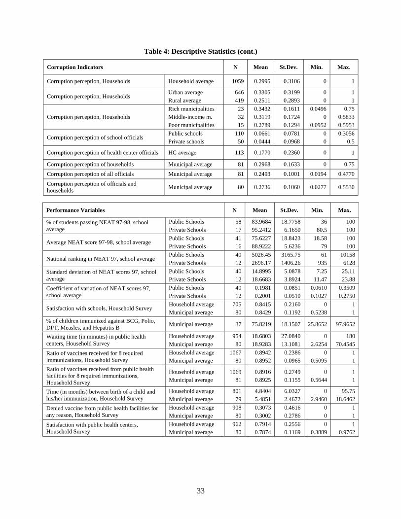
We begin by discussing our central variable of interest –corruption. We define corruption

as the abuse of office for personal gain (Klitgaard et al. (2000)). Corruption manifests itself in

several ways: through shirking, the sale of jobs, bribery, and the theft of funds and supplies. We

asked questions about all these improprieties in the surveys of government officials. Results are

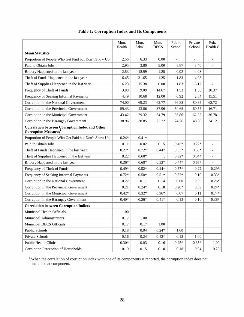
presented in Table 1. There are reports of all kinds of corruption in each kind of government

office –with the sole exception of the theft of supplies in the municipal education (DECS) office.

Most kinds of corruption are more prevalent in the municipal administrators office than in other

offices, perhaps due to the administrator’s office exerting more authority and thus having more

opportunity to extract rents (see Azfar and Gurgur 2000 for more on this subject). Nineteen

3 Barangay is the smallest political unit into which cities and municipalities in the Philippines are divided. It is thebasic unit of the Philippine political system. It often consists of less than 1,000 inhabitants residing within theterritorial limit of a city or municipality and administered by a set of elective officials, headed by a barangaychairman.

7

percent of municipal administrators stated that there were cases of bribery in their office in the

last year and a full 32% that there were instances of the theft of funds. By contrast only 2.5% of

municipal health officers and 1.3 % of municipal DECS officers reported incidents of bribery in

their office with 16.5% and 1.3%, respectively, reporting the theft of funds.

We next created an index of corruption from its various components. This index is the

normalized sum of the first seven variables in Table 1. This index is correlated at 0.5 or above

with most of its components for both the municipal administrator and the municipal DECS

officers. These high correlations, which reflect some positive link among the components of the

index, are the first sign that our index is measuring some coherent underlying variable.

We had also asked a general question on “how common is corruption in the municipal

government” with four possible answers: non-existent; rare; common; very common. If our

index were a good measure of corruption we would expect it to be correlated with the answer to

this question. In fact the indices are highly correlated with the answers to this general question

with a significance level of 5% or less for all municipal officials and officials at public health

centers.

Moreover the corruption perceptions of households and public officials are positively

correlated: We constructed a “public officials corruption index” combining the answers of public

officials working at public schools, health clinics and municipalities. The resulting index is

correlated at 0.28 (p-value=0.01) with households’ corruption perceptions.

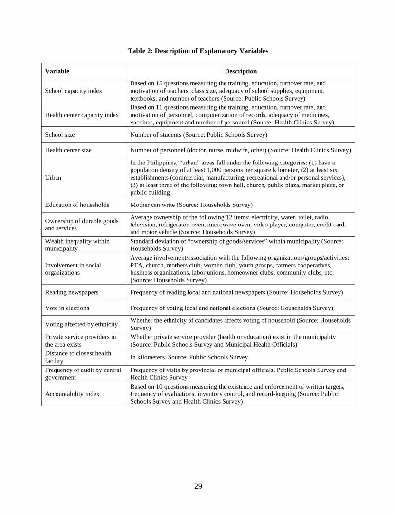
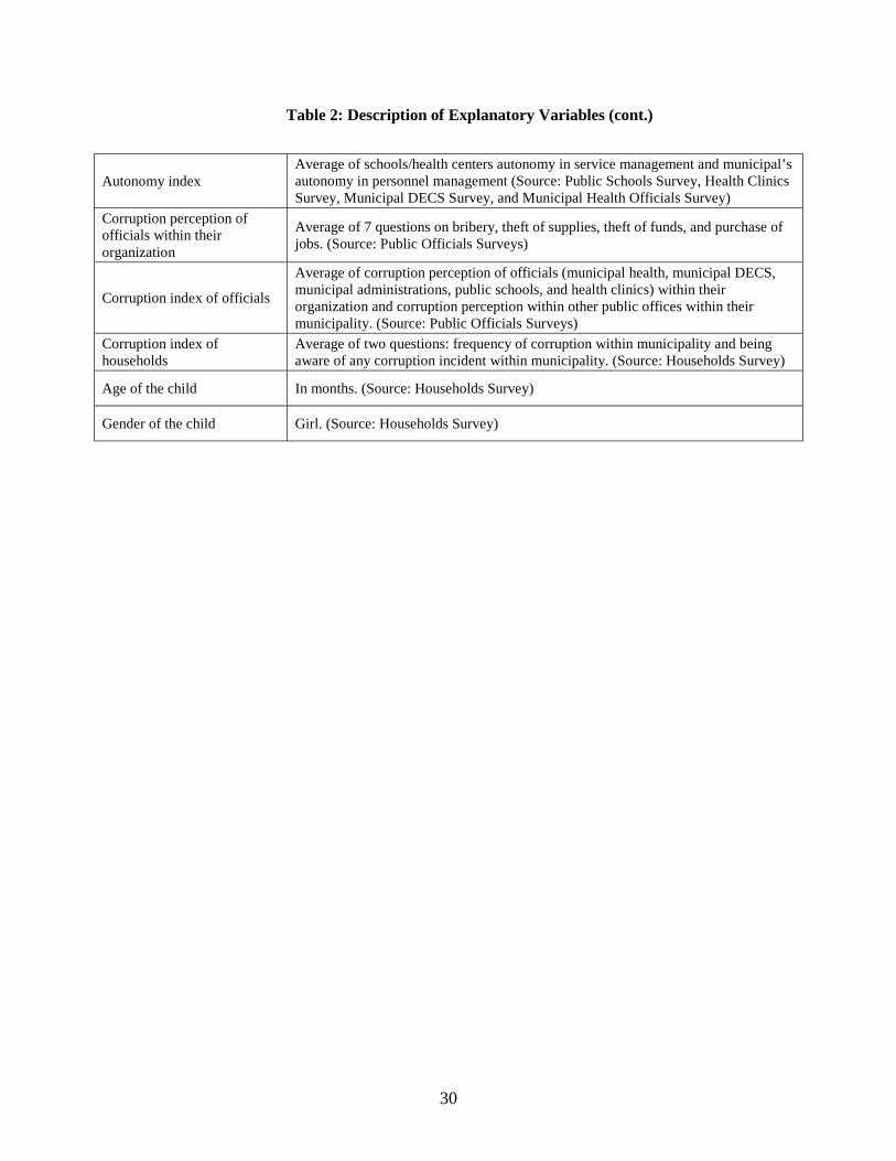
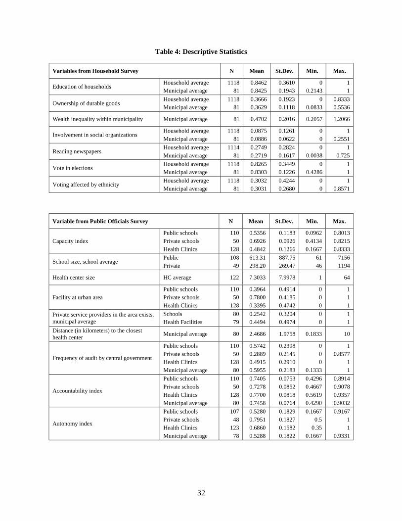
We also constructed measures of other aspects of public sector management and civic

community, which are categorized in three groups:

8

1. School/Health Center and Community Resources: physical and human resources of

schools or health centers (capacity index); size of school/ or health center, location

(urban area); education level of households; financial wealth of households

2. Voice, Exit, Civic Participation (social capital) variables: newspaper readership

among households; voter turn-out; effect of ethnicity in voting; existence of private

schools/health centers in the area; distance to closest health facility

3. Institutions: Internal accountability of schools, health facilities, and municipalities

(accountability index); frequency of audit by upper government; autonomy of

schools/health centers and municipalities in decision making

Most of these variables, which are described in Table 2, are composite indices between 0 and 1

and are constructed using several survey questions4.

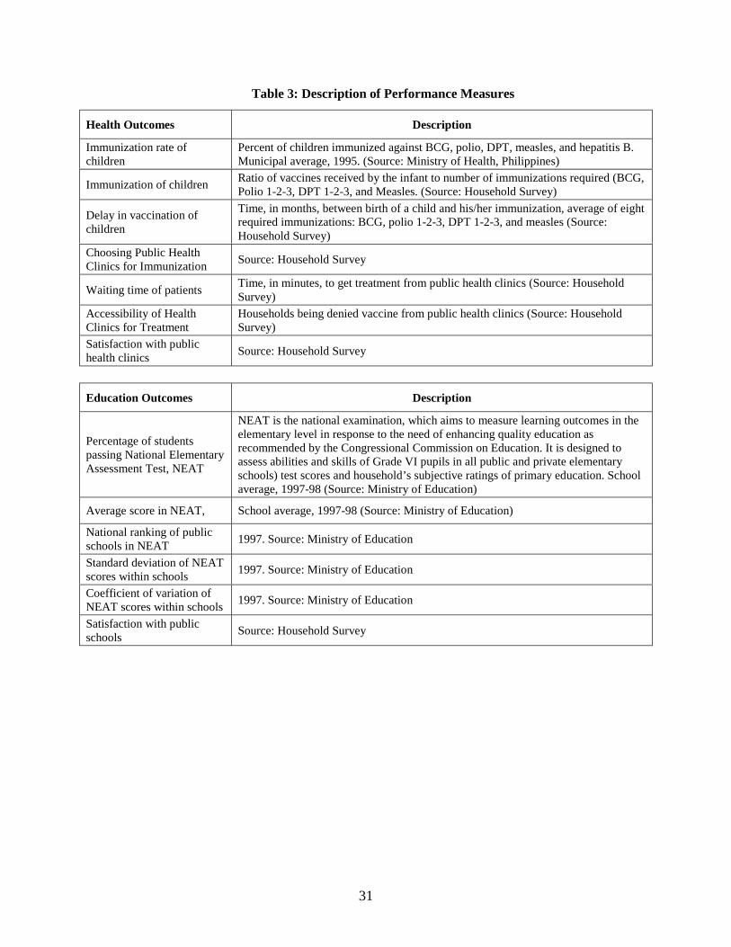
Our measures of performance in health and education services include both hard data

obtained from the Ministry of Health and the Ministry of Education in Philippines and users’

perceptions and responses that we derive from the Household Survey. These variables are

explained in Table 3.

IV. Econometric Model

We estimate the effect of corruption (as well as other variables) on performance of health

and education services using various methods, including random effect, tobit, ordinary-least

squares and robust regressions, at the household, school, and municipality level as appropriate.

The main justification for the random effects model is the individual units of analyses

(households) in our sample nested within higher-level units of analysis, which we identify as

4 An earlier draft entitled “Decentralization and corruption in the Philippines” contains tables that describe thesevariables in considerable detail and a number of reliability tests. This paper is available upon request.

9

provinces. A province in Philippines is the largest unit in the political structure, comprising of a

number of municipalities and (in some cases) cities with more or less homogenous

characteristics, such as ethnic origin of inhabitants, dialect spoken, agricultural produce, etc.

Therefore, it is possible that unobservable effects in each cross-section (province) may cause

biased estimates.

To address these concerns, we consider fixed-effects and random-effects models for

econometric analysis. As long as it is theoretically and statistically justified, a random effects

model is preferred to a fixed (within) effect model, since the latter ignores the information

offered by the comparison between provinces and consequently it is less efficient. However, an

important assumption behind random effects estimators is that random components of province-

specific effects are not correlated with the regressors. We test the appropriateness of this

assumption using Hausman test, which compares fixed effects estimators and random effects

estimators. Since fixed effects estimators are always consistent regardless of the orthogonality

condition, a significant difference between the estimates indicates correlation between the

regressors and the province-specific effects. If this is the case, we only report fixed effects

regression results. Otherwise, we use maximum-likelihood estimation that fully maximizes the

likelihood of the random-effects model. When our dependent variable is binary (e.g. use of

public health facilities), we use conditional logit and random-effects probit for fixed-effects and

random effects, respectively. In the latter, the likelihood is expressed as an integral computed

using Gauss-Hermite quadrature approximation and its numerical fitness is checked by re-

estimating the model with different quadrature points and comparing the change in estimates. If

the coefficients change by more than 1% the results are interpreted as unstable and not reported.

10

We should note that even when statistically justified, it is still theoretically debatable to

justify orthogonality between unobserved province-specific effects and explanatory variables,

since it is quite possible to imagine the confounding influence of these unobserved effects on at

least some regressors in the model (for example, a drug problem in one province may affect the

accountability or corruption variables). Hence, we always report estimates of fixed-effects model

along with random-effects results.

Almost in all cases we also try estimation via ordered probit method after transforming

continuous dependent variables, such as NEAT scores, school rankings, and standard deviation

of NEAT scores, into discrete ones. Although this approach lowers the information content of

dependent variables, the coefficient estimates are less likely to be affected by potential

measurement errors in dependent variables.

When our dependent variable is a performance measure based on government statistics,

the corresponding econometric model is either at school-level (e.g. test results) or at municipal-

level (e.g. immunization rate). When survey questions are used as dependent variables, we

estimate the model at the household level rather then aggregating the data in order to capture

household-specific effects, such as child characteristics, household income or education. We also

disaggregate the corruption variable based on location (urban vs. rural) and prosperity of

municipalities (rich, middle-income, and poor) to understand whether corruption affects one area

more or less than others depending on differences in regional characteristics.

11

V. Results

V.1 Health Outcomes

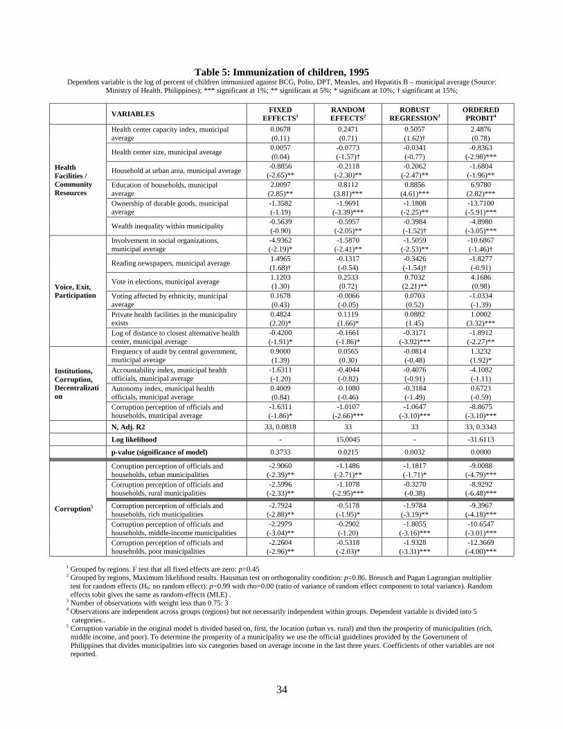
Our first performance measure is immunization coverage in the Philippines. The

regression model for percent of children immunized is at the municipal level since the Ministry

of Health provides data only on municipal averages. This limits our sample to 33 municipalities

(we lose several municipalities because of missing data). The results are presented in Table 5.

Local governments with high corruption level are less successful in providing immunization to

their communities. One standard deviation increase in corruption reduces immunization rate by

11-19 %5. The robustness of results to outliers is confirmed by the use of robust regression and

ordered probit models. Urbanization rates, unequal distribution of wealth, and distance to health

centers (as reported by public health facilities) also negatively influence immunization coverage.

Surprisingly, empirical results also indicate a negative partial correlation between immunization

and local prosperity, for which we have no easy explanation. We do not observe any difference

between rural vs. urban or rich vs. poor municipalities in terms of the effect of corruption. The

coefficients are usually significant and similar in magnitude.

Our next six dependent variables are derived from the Household survey and the

regressions are run at the household level. Although it is possible to run the same regressions at

more aggregate level (e.g. barangay or municipality), we prefer a household level analysis

because it allows us to use of household-level variables as regressors, such as child or household

characteristics. Additionally, to highlight the importance of community-specific variables, some

household level variables are aggregated at the municipal level. We, first, run regressions using

individual-specific variables alone (such as education, wealth, urbanization, social participation,

5 exp(1.6311 x 0.1060)-1= 0.1887 for fixed effects model; exp(1.0107 x 0.1060)-1 = 0.1131 for random effectsmodel

12

and reading newspapers) and then we add municipal averages of these variables to capture

community-specific effects.

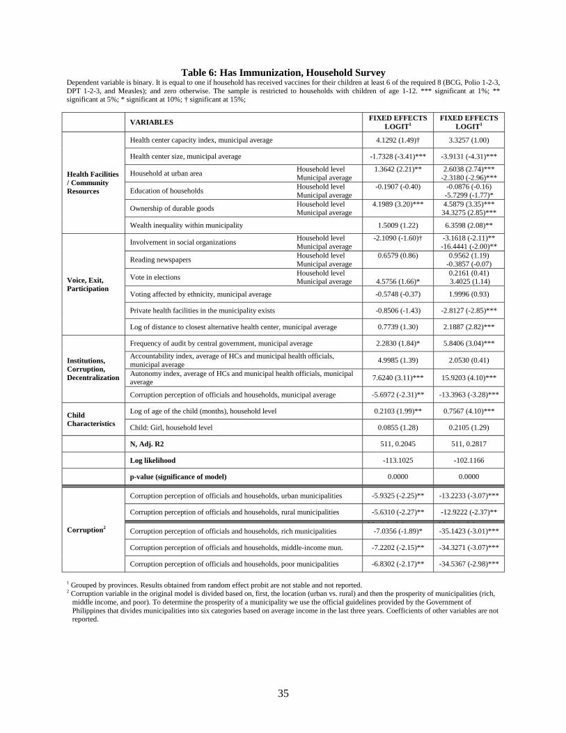
Regression results on vaccination of children (as reported by households) are presented in

Table 6. The sample is restricted to households with children of at least one year old. This

ensures that the households covered in our sample are the ones who should complete the

vaccinations of their children. The simple correlation between this variable and the previous

dependent variable is reasonably high (r = 0.46). The results show that the coefficient of

corruption variable is significant at 5% and its magnitude is quite substantial. The odds of

completing vaccination can decrease 1.8 to 4.2 times as a result of a one standard deviation

increase in corruption6. The size of public health facilities in the area has a negative impact on

immunization, suggesting that this variable is a proxy for excessive demand rather than adequate

supply (If governments respond to excess demand by increasing capacity, but less than is needed,

then larger facilities will be associated with more excess demand and hence lower immunization

rates. Another explanation is diseconomies of scale in the provision of vaccines). Unlike the

previous regression, this time wealth, rather than education of households, has a significant and

positive impact on immunization. Both the existence of private health providers and distance to

alternative public health facilities appear significant, albeit with wrong signs. It is possible that

both variables, similar to size of health facilities, are correlated with demand for health services.

Among public sector management variables, we find that the frequency of audit by central

government and autonomy of local governments increases the immunization coverage.

Next, we look at the causes of delay in vaccination of children. Our dependent variable is

the log of time (in months) between birth of a child and his/her immunization provided that the

child is at least one year old and that all immunizations have been completed. The variable is the

13

average of eight required immunizations (BCG, Polio 1-2-3, DPT 1-2-3, and Measles). The first

two columns in Table 7 are fixed-effects, followed by random effects model. Since there is an

inherent selection process in the dependent variable (i.e. dependent variable is observable only if

all vaccinations are completed), we also use Heckman's selection model to check sample

selection bias. However, we find that the correlation between the error terms of selection

equation and outcome equation is negligible (rho=0.01.) and the results of the outcome equation

are almost identical to ones obtained from fixed-effects model7. The corruption variable is

significant at 5% in all three columns. One standard deviation in corruption increases the time

between birth of a child and his/her immunization by 8-15%8. Existence of private health

facilities marginally reduces the length of this time period; distance to alternative health clinics,

on the other hand, has the opposite effect: infants are more likely to be vaccinated at later ages.

We also find that corruption is more damaging in rural municipalities as compared to urban ones,

but the difference is not statistically significant.

The regression results on choosing public health facilities for immunization are shown in

Table 8. As expected, wealth of a household is inversely proportional with his/her choosing

public health service over private ones. Households are also more likely to go to public health

clinics if wealth inequality in their municipality is higher or if there is no private health-service

providers in the area. We find that corruption in the public sector is an important deterrent that

discourages people to choose public health facilities. In areas where corruption is one standard

deviation lower than the national average, households are 2.77 times more likely to choose

6 1 / exp(-5.6972 x 0.1060) = 1.8292 from column (1) and 1 / exp(-13.3963 x 0.1060) = 4.1372 from column (2).7 177 observations are censored (households who have not yet completed vaccination of their children). Theselection equation involves all explanatory variables in the outcome equation, except the province dummies. Waldtest on independence of the equations (H0: rho=0): p=0.97. Average net marginal effect of corruption on dependentvariable (i.e. selection plus outcome): 1.1564 with standard deviation 0.0005.8 exp(0.7220 x 0.1060) -1= 0.0796 from column (3) and exp(1.3070 x 0.1060) -1 = 0.1486 from column (1).

14

public health facilities9. In poor municipalities, it is higher by as much as 7 folds10. We also use

Heckman's selection model to check whether the results are influenced by sample selection bias,

i.e. the decision to use public health facilities for immunization is influenced by households’

prior decision to immunize their children. We find that correlation between the error terms of

selection equation and outcome equation is very small (rho=0.01) and the results of the outcome

equation are almost identical to ones obtained from fixed-effects model11.

In Table 9 we study the waiting time (as reported by households) in public health clinics.

In addition to fixed-effects method, we also address sample selection issue using Heckman's

selection model since households may select themselves out of using public health clinics.

Although the correlation between selection and outcome processes is not significant, the

magnitude of the correlation (rho=0.11) is reasonably large and warrants reporting the results in

column (3). Due to concerns for perception bias on the behalf of households (that is, households

facing frequent delays would be suspicious of corruption in health facilities), we only use the

corruption perceptions of public officials our corruption measure. Corruption variable is

significant at 5 % when community-specific effects are not considered (first column), but

becomes only marginally significant when these effects are added to the model (column 2 and 3).

When we disaggregate the corruption variable based on location (urban vs. rural) and prosperity

of municipalities (rich, middle-income, and poor), we find that the influence of corruption on

waiting time is negligible in rich and/or urban communities. However, in rural regions one

9 exp(9.621 x 0.1060)=2.7727 from column (2).10 exp(18.3355 x 0.1094)=7.4328 from column (2).11 118 observations are censored (households who have not yet completed vaccination of their children). Theselection equation involves all explanatory variables in the outcome equation, except the province dummies. Waldtest on independence of the equations (H0: rho=0): p=0.95. Average net marginal effect of corruption on dependentvariable (i.e. selection plus outcome): -9.6211 with standard deviation 0.0005.

15

standard deviation in corruption can increase waiting time as much as 28% and in poor

municipalities 15%12.

In Table 10 we use the incidence of being denied a vaccine from public health facilities

(as reported by households). In addition to fixed- and random-effects model, we also use

Heckman's selection method, because the outcome variable is observable only if a household

chooses to use public health facilities. We again replace the composite corruption index with the

corruption perceptions of public officials, because the denial of a vaccine could affect a

household’s corruption perceptions. All estimation methods indicate that the corruption variable

is significant at 5% or less. A one standard deviation worsening in corruption may raise the

likelihood of being denied vaccines by 1.23-1.47 times13. In urban areas this increase is more

significant and can be as much as 2.13 fold14. Interestingly, the probability of being denied a

vaccine is positively related to the size of health facilities. As we discussed previously, the size

of health facilities is likely to be proportional to the demand for health services. The results also

show that patients are less likely to be denied a vaccine from public health clinics, if private

centers exist in the area or alternative private clinics are close enough.

Our last health-related performance variable is households' satisfaction with public health

clinics. Once again, in addition to fixed- and random-effects models, we use Heckman's selection

model to address sample selection problems (use of public health facilities is a prerequisite for

reporting satisfaction rating). Our corruption index excludes households' corruption perception.

The results, reported in Table 11, show that corruption has a statistically significant effect on

households' satisfaction with public health clinics. A one standard deviation improvement in

corruption can raise satisfaction ratings as much as 29% overall, 33% in rural areas and 48% in

12 exp(2.2428 x 0.1108)-1=0.2513 and exp(2.2428 x 0.1218)-1=0.1519 from column (1)13 exp(3.8730 x 0.1001)=1.4736 from column (2) and exp(2.0821 x 0.1001)=1.2317 from column (4).

16

poor municipalities15. We also find that the influence of corruption is slightly lower in urban

and/or rich municipalities, though the difference is not statistically significant.

In summary, our econometric analysis reveals that corruption has a significant and

negative effect on all health-related performance variables. In most cases the coefficient is

significant at 5 percent or less. The robustness of these results is checked using various

estimation techniques and different model specifications, which is discussed in the next section

in more detail. The corruption variable remains the single most important factor that influences

health outcomes in a consistent basis. We also find that demand for public health care is more

“corruption-elastic” in urban areas, i.e. corruption reduces households’ use of public health

facilities and the likelihood of getting vaccines from public clinics in urban areas, but it has less

influence over these two variables in rural areas. However, the effect of corruption on waiting

time in public health clinics is less significant in the urban areas. We attribute these results to the

presence of alternative health facilities in urban areas - either in the form of private health care

providers or other public health facilities. On the other hand, citizens in rural areas with rampant

corruption suffer with more waiting at public health clinics, late immunization of infants and

report less satisfaction with public health services.

We also run regressions to understand the effect of corruption in rich, middle-income and

poor municipalities. Regardless of the relative prosperity of a municipality, corruption hurts

satisfaction with public clinics, immunization rate of children, and average age of infants to get

vaccines. Poor and middle-income municipalities also report more waiting at public clinics and

more frequency of being denied vaccines when corruption is epidemic. Corruption in public

14 exp(7.9596 x 0.1001)=2.1217 from column (2).15 exp(2.5575 x 0.1001)=1.2901 from column (2); exp(3.0092 x 0.0945)=1.3289 from column (1), and exp(3.6137 x0.1094)=1.4849 from column (1).

17

clinics is also more likely to deter households living in poor municipalities from using public

clinics and forces them to opt for self-medication.

Our results also show that voting is not an effective mechanism to discipline local

governments –one possible explanation is that people might be voting on the basis of factors

other than improvements in service delivery. Exit mechanisms, in the form of existence of

private health facilities and accessibility of alternative health clinics, seem to have a more

significant impact, especially on the satisfaction with public health care, vaccinations of infants

at earlier ages, and accessibility of public health clinics for immunization. When it comes to

public sector management variables (accountability mechanisms, audit by central government,

and autonomy of local governments), we observe mixed results. The index that we constructed

for accountability of health facilities and municipalities remains insignificant in most regressions

and has wrong sign when it becomes significant. Audits by the central government have negative

effects on several health outcomes. Higher autonomy in local governments improves

immunization rate (as reported by households), raises accessibility of public health facilities for

immunization and reduces the time length between birth of an infant and his/her immunization,

but it also leads to longer waiting times.

V.2 Education

Next, we look at the education-related performance variables. All econometric models,

except households’ satisfaction ratings, are at barangay levels.

We start with households' satisfaction with public schools. The results are reported in

Table 12. The estimation methods we use include fixed- and random-effects to capture region-

specific factors, as well as Heckman's selection method to address school selection process that

18

precedes satisfaction ratings. As we did before, we exclude households' opinion on corruption

and use only public officials' perceptions to prevent a biased link between the dependent variable

and the regressor. We find that the corruption variable appears significant at 5% in random-

effects model, but only marginally significant in fixed-effects and Heckman's selection models.

The results do not show any statistically significant partial correlation between corruption and

households' satisfaction with public schools in urban areas or rich municipalities. Existence of

private schools in the area and frequency of reading newspapers are two other variables with

significantly negative influence over schools' satisfaction ratings. It is possible that both

variables enable households to compare the performance of their schools with alternatives and

make them more critical in their assessments.

Next, we move to more objective education outcomes in public schools. Dependent

variables are at the school level and they include various measures of success in a nation-wide

exam (NEAT). The most obvious measure of the quality of service delivery is the mean of the

NEAT score and the closely related school ranking. Variation of students' test scores within a

school is another outcome variable. It shows whether a school is able to provide equal

opportunity to its students to achieve their potential. We measure variation in terms of standard

deviation of test results. However, since the standard deviation of a variable is likely to be

proportional to its mean, we also use the coefficient of variation (standard deviation divided by

the sample average) as another measure of variance.

The results on percentage of student passing NEAT are presented in Table 13. We find

that corruption in the public sector, in particular in rural municipalities, significantly reduces the

success rate of students. A one standard deterioration in corruption around its mean causes a 12%

decrease in number of students passing NEAT. There is no evidence that the effect of corruption

19

differs between affluent municipalities and poor municipalities. Among other significant

variables we find that schools with better financial and personnel capacity are able to raise the

percentage of students passing NEAT. Barangays with better-educated households also witness

better test scores –this may represent a parent-child human capital transfer. Higher voter turnout

pushes test scores up, whereas influence of ethnicity in elections and wealth inequality within

municipalities hurt education results. Exit mechanisms (existence of private schools in the area),

accountability mechanisms, and audit by central government are mostly ineffective.

As shown in Table 14 average NEAT scores of students are also adversely affected by

corruption in public sector. A one standard increase in corruption reduces NEAT scores as much

as 11%. Comparing the effect of corruption in rich and poor municipalities, we observe that

corruption has slightly more negative effect in rich municipalities. Education of parents and

autonomy of public schools in decision-making are found to improve test scores, whereas wealth

inequality and voting based on ethnicity reduces school performance.

Another outcome variable that we used in our regressions is the national ranking of

schools based on NEAT scores (Table 15). The effect of corruption is even more striking: a one

standard deviation increase in corruption increases school ranking as much as 93% (higher ranks

correspond to worse performance). Corruption is especially damaging in rural areas, where the

magnitude of corruption coefficient is 2-3 larger.

In addition to performance variables measuring level of success in NEAT scores, we also

look at the variation of scores within schools. As shown in Table 16, the standard deviation of

NEAT scores rises where corruption is more persistent, especially in rural areas. The other two

significant variables are school capacity index and ethnic divisions (proxied by ethnicity

considerations in voting decisions). Schools that enjoy better financial and personnel resources

20

are produce less equal outcomes. One possible explanation is that better off parents are more

motivated to capture resources when capacity is higher. Pervasiveness of ethnic divisions in

communities also has a similar effect. Since it is possible that standard deviation of test scores

may be inflated by higher test scores, we also look at the coefficient of variation, which divides

sample standard deviation by sample average. The results, reported in Table 17, are similar.

Corruption and voting based on ethnicity have still negative impact on education outcomes.

Capacity also appears to be related to greater inequality in outcomes.

VI. Robustness

VI.1 Selection

We have shown that there is a significant partial correlation between 13 dependant

variables that measure various aspects of health and education services and corruption

perceptions, after controlling for capacity (based on measures of human and physical capital),

adult education levels, urban residence, living standards (as proxied by assets), inequality,

existence of private sector competition, voting and media exposure, accountability measures, and

local autonomy.

To check the robustness of the regression results we use a robust regression method that

involves down weighing observations that resemble outliers. It begins by estimating the

regression, calculating Cook’s D distance statistics and excluding any observation with D>1.

After that a weight is assigned to each observation inversely proportional to its residual. The

appropriateness of this robust regression method may be questionable as the number of

observations with small weights increases (we report the portion of the sample with weights less

than 0.75). As one can see from the regression tables, robust estimates are very close to the ones

21

we obtain from other estimation methods. Hence, we conclude that our results are not greatly

influenced by any outlier in the sample.

Another concern that we address is the sample selection problem. When we regress, for

example, waiting time in public health clinics or satisfaction with public schools on a set of

explanatory variables, the sample space is limited with households that choose public service

providers over the private ones. When such a selection process exists, linear regression estimates

have to be adjusted for the fact that the dependent variable is the outcome of a nonrandom

selection process. To tackle the issue of sample selection bias in regression results, we use

Heckman’s selection method (Heckman (1979)). The basic idea of a sample selection model is

that the outcome variable, y, is only observed if some criterion, defined with respect to a variable

z, is met. The original Heckman’s method involves a two-stage approach: In the first stage, a

dichotomous variable z determines whether or not y is observed; in the second state, the outcome

variable y is estimated conditional on its being observed. The two error terms corresponding to

selection equation and outcome equation are assumed to be correlated and having a joint

bivariate normal distribution. We estimate the parameters by fully maximizing the joint

likelihood function, which takes into account the heteroscedasticity of the error terms16. These

estimates are consistent and asymptotically efficient under the assumption of normality17. The

similarity in results, in particular for the coefficient of corruption variable, reinforces our conclusion

that the negative and significant effect of corruption on health and education outcomes does not arise

from a selection process.

16 Note that if a variable appears in both the selection and outcome equations the coefficient in the outcome equationis affected by its presence in the selection equation as well. Therefore, after reporting the estimates for outcomeequation, as a footnote we also report the net effect of corruption variable that takes into account its effect inselection process17 However, if the normality assumption is violated or there is a model specification error in one of the equations,then the estimated will be biased. For that reason, we choose to use other estimation methods instead of solelyreporting the results obtained from Heckman’s selection method.

22

VI.2 Causality

Another concern in econometric studies is about whether the partial correlation reflects a

genuine causal relationship. For example, poor service delivery may be a cause of corruption in

the public sector, as well as being a consequence. It is also possible that some common source of

respondent bias, like pessimism about the performance public sector, has led to worse

perceptions of corruption. To tackle these problems, we use four approaches:

First, to correct potential “cynicism” of respondents towards government and the

corruption level, we used a survey question that is supposed to be answered similarly (in the

absence of individual bias) by all respondents: “the extent of corruption in central government”.

We assumed that the average score represents the true corruption level in central government and

thus, the difference between a person’s responds and the average score reflects the “pessimism”

or “optimism” of that person. Using that difference as a discount factor, we updated the

corruption index . We found that perceptions on national corruption is highly correlated with

perceptions on local corruption (r = 0.3010, significant at 1%).

Second, we applied the standard statistical approach to resolve the reverse causality

problem by using instrumental variables. Following Mauro (1997) and Friedman et al. (2000),

we used the ethnic fragmentation at each municipality as an instrument for corruption at that

municipality. The ethnolinguistic fractionalization variable was computed as one minus the

Herfindahl index of ethnolinguistic group shares, and reflected the probability that two randomly

selected individuals from a population belonged to different groups18. The data for both variables

were obtained from the 2000 Census of Population. As an additional instrument we also used a

survey question that measures the extent to which ethnicity affects voting in local elections.

18 The exact formula is 21 ii

s−∑ where si is the share of group i in the jurisdiction.

23

Simple correlations between these two variables and the corruption index are 0.41 and 0.47,

respectively. The R square at the first stage was 0.37. We corroborated the validity of the

instruments with an OIR-Hausman test19.

In our third approach, we transformed the dependent variables into zero to one interval,

which enabled logit specification. Then, instead of trying to find an instrument that is

conceptually linked to corruption, we used the polynomials of exogenous variables as

instruments thanks to non-linear estimation required by logit specification20. The R square at the

first stage was 0.65. We verified the validity of overidentifying restrictions using Hausman test21.

The results are summarized and compared with the results from the base models in Table

18. In general, when a dependent variable is based on objective sources (such as test scores)

rather than subjective sources (such as satisfaction with public schools) the results are quite

similar in magnitude and significance level. For example, according to our base results a 10

percent increase in corruption reduces immunization rates (as reported by the Ministry of Health)

3.6-3.8 percent. When IV approach is used, that figure is in the range of 2.2-3.0 percent. When a

dependent variable reflects the observations of households, the results that are based on

“cleaned” corruption perceptions somewhat differ from the base results: the magnitudes of the

coefficients are lower and their statistical significance is a little weaker. Overall 9 out of 13

coefficients remain significant at 5% if the “cleaned” corruption variable is used. IV results, on

19 The test is based on regressing the residuals from the main structural equation on the entire set of exogenousvariables. Under the null hypothesis of overidentifying restrictions, the test statistic, NR2 (N is the sample size andR2 is the uncentered the goodness of fit from the regression of residuals on all the instruments) has a χ2 distributionwith K-T degrees of freedom, where K is the number of exogenous variables and T is the number of endogenousvariables. If the instruments are excluded from the structural equation correctly, the set of instruments should haveno explaining power over the residuals and consequently R2 should be low. The p-value of the test statistic is 0.76for ethnic fragmentation and 0.52 for the ethnic voting. Hence, we failed to reject the null hypothesis that theoveridenfying restrictions are valid.20 Some dependent variables (such as test scores or immunization rates) can easily be transformed to 0-1 interval bydividing by 100. For some other variables (such as ranking in NEAT), we divided the observations by theirmaximum.

24

the other hand, are still closer to the base results, suggesting that reverse causality is not serious

problem.

VII. Conclusion

In this paper we used data from 80 municipalities in the Philippines to assess the impact

of corruption in local governments on health and education outcomes.

Our results showed clearly that corruption undermines the delivery of health services in

the Philippines. We used seven different measures for the quality of health services: six of them

from Household Survey (immunization of children, delay in vaccination of children, waiting

time of patients, accessibility of health clinics for treatment, choosing public health clinics for

immunization, and satisfaction with public health clinics) and one from the Ministry of Health

(municipal average of immunization rate of children). In each case regression results indicated a

significant and negative effect of corruption on the quality of health services. We also found that

corruption affects health outcomes in rural areas in a different way than the urban areas. Demand

for public health care is more “corruption-elastic” in the urban areas, whereas rural areas with

rampant corruption suffer with more waiting at public health clinics, late immunization of

infants, and less satisfaction with public health services.

There are also important poverty relevant effects. Regardless of the prosperity of a

municipality, corruption hurts satisfaction with public clinics, immunization rate of children, and

leads to delays in vaccinations (the magnitude of this effect is more significant in poor

municipalities). However, unlike rich municipalities, poor and middle-income municipalities also

report more waiting at public clinics and a higher frequency of being denied of vaccines when

21 The p-value of the test statistic was between 0.59 and 0.91 depending on the instrument tested.

25

corruption is widespread. Corruption in public clinics is also more likely to deter households

living in poor municipalities and forces them to opt for self-medication.

Our results on education were similar. We used seven measures for the quality of

education: various measures of test scores and household assessments of the quality of education.

Corruption hurts all education outcomes. However, its negative effect is more prevalent in rural

areas than the urban. We observed, on the other hand, minor differences between rich and poor

municipalities in terms of the effects of corruption. The coefficients of corruption variables are

significant in both cases and similar in magnitude

Taken together our results do suggest that corruption undermines the delivery of health

and education. This complements cross-country findings on the subject, and adds to the

expanding list of ways corruption undermines welfare.

26

References

Acemoglu, D., Johnson S., Robinson, J. A. (2001) Colonial origins of comparativedevelopment: An empirical investigation. American Economic Review 91: 1369-1401

Azfar, O. (2003) Review of corruption and the delivery of health and education services.Mimeo., IRIS, University of Maryland, College Park

Azfar, O., Gurgur, T (2000) Decentralization and corruption in the Philippines. Mimeo., IRIS,University of Maryland, College Park

Azfar, O., Gurgur, T., Meagher, P. (2004) Political disciplines on local government: Evidencefrom the Philippines. In M. S. Kimenyi and P. Meagher (ed) Devolution andDevelopment, Governance Prospects in Decentralizing States. London, Ashagate

Batalla, E. (2000) The social cancer: Corruption as a way of life. Philippine Daily Inquirer,August 27

Department of Interior, Philippines, Local Government Code of 1991, Republic Act No. 7160,Department of Interior and Local Government, Manila

Friedman, E., Johnson, S., Kaufmann, D., Zoido-Lobaton, P. (2000) Dodging the grabbing hand:the determinants of unofficial activity in 69 countries. Journal Of Public Economics 76(3): 459-493

Gray-Molina G., De Rada E. P., Yánez E. (1999) Transparency and accountability in Bolivia:Does voice matter?. Working Paper No. R-381, Inter-American Development Bank,Washington, D.C.

Guerrero, L.L., Rood, S. A. (1999) An explanatory study of graft and corruption in thePhilippines. Social Science Information 27(1): 110-141

Gupta, S., Verhoeven, M., Tiongson, E. (2002) The effectiveness of government spending oneducation and healthcare in developing and transition countries. European Journal ofPolitical Economy 18: 717-737

Klitgaard, R., MacLean-Abaroa, R., Parris, H.L. (2000) Corrupt Cities: A Practical Guide toCure and Prevention, Boston, ICS Press

Heckman, J (1979) Sample selection bias as a specification error. Econometrica 47: 153-161

Manasan, R. (1997) Local government financing of social service sectors in a decentralizedregime: Special focus on provincial governments in 1993 and 1994. Discussion Paper97-04, Philippine Institute for Development Studies, Manila

Mauro, Paolo (1997) Corruption and growth. Quarterly Journal of Economics 110(3): 681-712

27

Miller, T. (1997) Fiscal federalism in theory and practice: The Philippines Case. USAIDEconomists Working Papers Series No. 4, Washington, D.C.

Pritchett, L. (1996) Mind your P’s and Q’s: The cost of public investment is not the value ofpublic capital. Policy Research Working Paper 1660, World Bank, Washington, D.C.

Rajkumar, A.S., Swaroop, V. (2002) Public spending and outcomes: Does governance matter?Mimeo., World Bank, Washington, D.C.

Reinikka, R., Svensson, J. (2001) Explaining leakage of public funds. World Bank PolicyResearch Paper 2709, Washington, D.C.

World Bank (1994) The Philippines Devolution and Health Services: Managing Risks andOpportunities, Washington, D.C.

World Bank (2000) Combating Corruption in the Philippines, Washington D.C.

28

Table 1: Corruption Index and Its Components

Mun.Health

Mun.Adm..

Mun.DECS

PublicSchool

PrivateSchool

Pub.Health C

Mean StatisticsProportion of People Who Get Paid but Don’t Show Up 2.56 6.33 0.00 - - -Paid to Obtain Jobs 2.95 3.80 5.00 8.87 3.40 -Bribery Happened in the last year 2.53 18.99 1.25 0.92 4.08 -Theft of Funds Happened in the last year 16.45 31.65 1.25 1.83 4.08 -Theft of Supplies Happened in the last year 16.23 15.38 0.00 1.83 6.12 -Frequency of Theft of Funds 3.80 9.09 14.67 1.53 1.36 20.37Frequency of Seeking Informal Payments 4.49 10.68 12.00 0.92 2.04 15.51Corruption in the National Government 74.00 69.23 62.77 66.35 80.85 62.72Corruption in the Provincial Government 59.43 43.86 37.96 50.65 69.57 46.71Corruption in the Municipal Government 43.42 29.32 24.79 36.86 62.32 36.78Corruption in the Barangay Government 38.96 28.85 22.22 24.76 48.89 24.12

Correlation between Corruption Index and OtherCorruption Measures1

Proportion of People Who Get Paid but Don’t Show Up 0.24* 0.41* - - - -Paid to Obtain Jobs 0.11 0.02 0.15 0.45* 0.22* -Theft of Funds Happened in the last year 0.27* 0.72* 0.44* 0.53* 0.68* -Theft of Supplies Happened in the last year 0.22 0.68* . 0.32* 0.64* -Bribery Happened in the last year 0.26* 0.68* 0.52* 0.44* 0.65* -Frequency of Theft of Funds 0.49* 0.52* 0.44* 0.37* 0.22 0.29*Frequency of Seeking Informal Payments 0.72* 0.50* 0.51* 0.32* 0.10 0.33*Corruption in the National Government 0.22 0.11 0.14 0.00 0.09 0.26*Corruption in the Provincial Government 0.21 0.24* 0.18 0.20* 0.09 0.24*Corruption in the Municipal Government 0.42* 0.32* 0.36* 0.07 0.11 0.74*Corruption in the Barangay Government 0.40* 0.26* 0.41* 0.13 0.10 0.36*Correlation between Corruption IndicesMunicipal Health Officials 1.00Municipal Administrators 0.17 1.00Municipal DECS Officials 0.17 0.17 1.00Public Schools 0.18 0.04 0.24* 1.00Private Schools 0.16 0.24 0.42* 0.13 1.00Public Health Clinics 0.30* 0.03 0.16 0.25* 0.35* 1.00Corruption Perception of Households 0.19 0.15 0.18 0.18 0.04 0.20

1 When the correlation of corruption index with one of its components is reported, the corruption index does notinclude that component.

29

Table 2: Description of Explanatory Variables

Variable Description

School capacity indexBased on 15 questions measuring the training, education, turnover rate, andmotivation of teachers, class size, adequacy of school supplies, equipment,textbooks, and number of teachers (Source: Public Schools Survey)

Health center capacity indexBased on 11 questions measuring the training, education, turnover rate, andmotivation of personnel, computerization of records, adequacy of medicines,vaccines, equipment and number of personnel (Source: Health Clinics Survey)

School size Number of students (Source: Public Schools Survey)

Health center size Number of personnel (doctor, nurse, midwife, other) (Source: Health Clinics Survey)

Urban

In the Philippines, “urban” areas fall under the following categories: (1) have apopulation density of at least 1,000 persons per square kilometer, (2) at least sixestablishments (commercial, manufacturing, recreational and/or personal services),(3) at least three of the following: town hall, church, public plaza, market place, orpublic building

Education of households Mother can write (Source: Households Survey)

Ownership of durable goodsand services

Average ownership of the following 12 items: electricity, water, toilet, radio,television, refrigerator, oven, microwave oven, video player, computer, credit card,and motor vehicle (Source: Households Survey)

Wealth inequality withinmunicipality

Standard deviation of “ownership of goods/services” within municipality (Source:Households Survey)

Involvement in socialorganizations

Average involvement/association with the following organizations/groups/activities:PTA, church, mothers club, women club, youth groups, farmers cooperatives,business organizations, labor unions, homeowner clubs, community clubs, etc.(Source: Households Survey)

Reading newspapers Frequency of reading local and national newspapers (Source: Households Survey)

Vote in elections Frequency of voting local and national elections (Source: Households Survey)

Voting affected by ethnicity Whether the ethnicity of candidates affects voting of household (Source: HouseholdsSurvey)

Private service providers inthe area exists

Whether private service provider (health or education) exist in the municipality(Source: Public Schools Survey and Municipal Health Officials)

Distance to closest healthfacility In kilometers. Source: Public Schools Survey

Frequency of audit by centralgovernment

Frequency of visits by provincial or municipal officials. Public Schools Survey andHealth Clinics Survey

Accountability indexBased on 10 questions measuring the existence and enforcement of written targets,frequency of evaluations, inventory control, and record-keeping (Source: PublicSchools Survey and Health Clinics Survey)

30

Table 2: Description of Explanatory Variables (cont.)

Autonomy indexAverage of schools/health centers autonomy in service management and municipal’sautonomy in personnel management (Source: Public Schools Survey, Health ClinicsSurvey, Municipal DECS Survey, and Municipal Health Officials Survey)

Corruption perception ofofficials within theirorganization

Average of 7 questions on bribery, theft of supplies, theft of funds, and purchase ofjobs. (Source: Public Officials Surveys)

Corruption index of officials

Average of corruption perception of officials (municipal health, municipal DECS,municipal administrations, public schools, and health clinics) within theirorganization and corruption perception within other public offices within theirmunicipality. (Source: Public Officials Surveys)

Corruption index ofhouseholds

Average of two questions: frequency of corruption within municipality and beingaware of any corruption incident within municipality. (Source: Households Survey)

Age of the child In months. (Source: Households Survey)

Gender of the child Girl. (Source: Households Survey)

31

Table 3: Description of Performance Measures

Health Outcomes Description

Immunization rate ofchildren

Percent of children immunized against BCG, polio, DPT, measles, and hepatitis B.Municipal average, 1995. (Source: Ministry of Health, Philippines)

Immunization of children Ratio of vaccines received by the infant to number of immunizations required (BCG,Polio 1-2-3, DPT 1-2-3, and Measles. (Source: Household Survey)

Delay in vaccination ofchildren

Time, in months, between birth of a child and his/her immunization, average of eightrequired immunizations: BCG, polio 1-2-3, DPT 1-2-3, and measles (Source:Household Survey)

Choosing Public HealthClinics for Immunization Source: Household Survey

Waiting time of patients Time, in minutes, to get treatment from public health clinics (Source: HouseholdSurvey)

Accessibility of HealthClinics for Treatment

Households being denied vaccine from public health clinics (Source: HouseholdSurvey)

Satisfaction with publichealth clinics Source: Household Survey

Education Outcomes Description

Percentage of studentspassing National ElementaryAssessment Test, NEAT

NEAT is the national examination, which aims to measure learning outcomes in theelementary level in response to the need of enhancing quality education asrecommended by the Congressional Commission on Education. It is designed toassess abilities and skills of Grade VI pupils in all public and private elementaryschools) test scores and household’s subjective ratings of primary education. Schoolaverage, 1997-98 (Source: Ministry of Education)

Average score in NEAT, School average, 1997-98 (Source: Ministry of Education)

National ranking of publicschools in NEAT 1997. Source: Ministry of Education

Standard deviation of NEATscores within schools 1997. Source: Ministry of Education

Coefficient of variation ofNEAT scores within schools 1997. Source: Ministry of Education

Satisfaction with publicschools Source: Household Survey

32

Table 4: Descriptive Statistics

Variables from Household Survey N Mean St.Dev. Min. Max.

Education of householdsHousehold averageMunicipal average

111881

0.84620.8425

0.36100.1943

00.2143

11

Ownership of durable goodsHousehold averageMunicipal average

111881

0.36660.3629

0.19230.1118

00.0833

0.83330.5536

Wealth inequality within municipality Municipal average 81 0.4702 0.2016 0.2057 1.2066

Involvement in social organizationsHousehold averageMunicipal average

111881

0.08750.0886

0.12610.0622

00

10.2551

Reading newspapersHousehold averageMunicipal average

111481

0.27490.2719

0.28240.1617

00.0038

10.725

Vote in electionsHousehold averageMunicipal average

111881

0.82650.8303

0.34490.1226

00.4286

11

Voting affected by ethnicityHousehold averageMunicipal average

111881

0.30320.3031

0.42440.2680

00

10.8571

Variable from Public Officials Survey N Mean St.Dev. Min. Max.

Capacity indexPublic schoolsPrivate schoolsHealth Clinics

11050

128

0.53560.69260.4842

0.11830.09260.1266

0.09620.41340.1667

0.80130.82150.8333

School size, school averagePublicPrivate

10849

613.31298.20

887.75269.47

6146

71561194

Health center size HC average 122 7.3033 7.9978 1 64

Facility at urban areaPublic schoolsPrivate schoolsHealth Clinics

11050

128

0.39640.78000.3395

0.49140.41850.4742

000

111

Private service providers in the area exists,municipal average

SchoolsHealth Facilities

8079

0.25420.4494

0.32040.4974

00

11

Distance (in kilometers) to the closesthealth center Municipal average 80 2.4686 1.9758 0.1833 10

Frequency of audit by central government

Public schoolsPrivate schoolsHealth ClinicsMunicipal average

11050

12880

0.57420.28890.49150.5955

0.23980.21450.29100.2183

000

0.1333

10.8577

11

Accountability index


11050

12880

0.74050.72780.77000.7458

0.07530.08520.08180.0764

0.42960.46670.56190.4290

0.89140.90780.93570.9032

Autonomy index


10748

12378

0.52800.79510.68600.5288

0.18290.18270.15820.1822

0.16670.5

0.350.1667

0.916711

0.9331

33

Table 4: Descriptive Statistics (cont.)

Corruption Indicators N Mean St.Dev. Min. Max.

Corruption perception, Households Household average 1059 0.2995 0.3106 0 1

Corruption perception, HouseholdsUrban averageRural average

646419

0.33050.2511

0.31990.2893

00

11

Corruption perception, HouseholdsRich municipalitiesMiddle-income m.Poor municipalities

233215

0.34320.31190.2789

0.16110.17240.1294

0.04960

0.0952

0.750.58330.5953

Corruption perception of school officialsPublic schoolsPrivate schools

11050

0.06610.0444

0.07810.0968

00

0.30560.5

Corruption perception of health center officials HC average 113 0.1770 0.2360 0 1

Corruption perception of households Municipal average 81 0.2968 0.1633 0 0.75Corruption perception of all officials Municipal average 81 0.2493 0.1001 0.0194 0.4770

Corruption perception of officials andhouseholds Municipal average 80 0.2736 0.1060 0.0277 0.5530

Performance Variables N Mean St.Dev. Min. Max.

% of students passing NEAT 97-98, schoolaverage

Public SchoolsPrivate Schools

5817

83.968495.2412

18.77586.1650

3680.5

100100

Average NEAT score 97-98, school averagePublic SchoolsPrivate Schools

4116

75.622788.9222

18.84235.6236

18.5879

100100

National ranking in NEAT 97, school averagePublic SchoolsPrivate Schools

4012

5026.452696.17

3165.751406.26

61935

101586128

Standard deviation of NEAT scores 97, schoolaverage


4012

14.899518.6683

5.08783.8924

7.2511.47

25.1123.88

Coefficient of variation of NEAT scores 97,school average


4012

0.19810.2001

0.08510.0510

0.06100.1027

0.35090.2750

Satisfaction with schools, Household SurveyHousehold averageMunicipal average

70580

0.84150.8429

0.21600.1192

00.5238

11

% of children immunized against BCG, Polio,DPT, Measles, and Hepatitis B Municipal average 37 75.8219 18.1507 25.8652 97.9652

Waiting time (in minutes) in public healthcenters, Household Survey

Household averageMunicipal average

95480

18.680318.9283

27.084013.1081

02.6254

18070.4545

Ratio of vaccines received for 8 requiredimmunizations, Household Survey


106780

0.89420.8952

0.23860.0965

00.5095

11

Ratio of vaccines received from public healthfacilities for 8 required immunizations,Household Survey


106981

0.89160.8925

0.27490.1155

00.5644

11

Time (in months) between birth of a child andhis/her immunization, Household Survey


80179

4.84045.4851

6.03272.4672

02.9460

95.7518.6462

Denied vaccine from public health facilities forany reason, Household Survey


90880

0.30730.3002

0.46160.2786

00

11

Satisfaction with public health centers,Household Survey


96280

0.79140.7874

0.25560.1169

00.3889

10.9762

34

Table 5: Immunization of children, 1995Dependent variable is the log of percent of children immunized against BCG, Polio, DPT, Measles, and Hepatitis B – municipal average (Source:

Ministry of Health, Philippines); *** significant at 1%; ** significant at 5%; * significant at 10%; † significant at 15%;

VARIABLES FIXEDEFFECTS1

RANDOMEFFECTS2

ROBUSTREGRESSION3

ORDEREDPROBIT4

Health center capacity index, municipalaverage

0.0678(0.11)

0.2471(0.71)

0.5057(1.62)†

2.4876(0.78)

Health center size, municipal average 0.0057(0.04)

-0.0773(-1.57)†

-0.0341(-0.77)

-0.8363(-2.98)***

Household at urban area, municipal average -0.8856(-2.65)**

-0.2118(-2.30)**

-0.2062(-2.47)**

-1.6804(-1.96)**

Education of households, municipalaverage

2.0097(2.85)**

0.8112(3.81)***

0.8856(4.61)***

6.9780(2.82)***

Ownership of durable goods, municipalaverage

-1.3582(-1.19)

-1.9691(-3.39)***

-1.1808(-2.25)**

-13.7100(-5.91)***

HealthFacilities /CommunityResources

Wealth inequality within municipality -0.5639(-0.90)

-0.5957(-2.05)**

-0.3984(-1.52)†

-4.8980(-3.05)***

Involvement in social organizations,municipal average

-4.9362(-2.19)*

-1.5870(-2.41)**

-1.5059(-2.53)**

-10.6867(-1.46)†

Reading newspapers, municipal average 1.4965(1.68)†

-0.1317(-0.54)

-0.3426(-1.54)†

-1.8277(-0.91)

Vote in elections, municipal average 1.1203(1.30)

0.2533(0.72)

0.7032(2.21)**

4.1686(0.98)

Voting affected by ethnicity, municipalaverage

0.1678(0.43)

-0.0066(-0.05)

0.0703(0.52)

-1.0334(-1.39)

Private health facilities in the municipalityexists

0.4824(2.20)*

0.1119(1.66)*

0.0882(1.45)

1.0002(3.32)***

Voice, Exit,Participation

Log of distance to closest alternative healthcenter, municipal average

-0.4200(-1.91)*

-0.1661(-1.86)*

-0.3171(-3.92)***

-1.8912(-2.27)**

Frequency of audit by central government,municipal average

0.9000(1.39)

0.0565(0.30)

-0.0814(-0.48)

1.3232(1.92)*

Accountability index, municipal healthofficials, municipal average

-1.6311(-1.20)

-0.4044(-0.82)

-0.4076(-0.91)

-4.1082(-1.11)

Autonomy index, municipal healthofficials, municipal average

0.4009(0.84)

-0.1080(-0.46)

-0.3184(-1.49)

0.6723(-0.59)

Institutions,Corruption,Decentralization

Corruption perception of officials andhouseholds, municipal average

-1.6311(-1.86)*

-1.0107(-2.66)***

-1.0647(-3.10)***

-8.8675(-3.10)***

N, Adj. R2 33, 0.0818 33 33 33, 0.3343

Log likelihood - 15.0045 - -31.6113

p-value (significance of model) 0.3733 0.0215 0.0032 0.0000

Corruption perception of officials andhouseholds, urban municipalities

-2.9060(-2.39)**

-1.1486(-2.71)**

-1.1817(-1.71)*

-9.0088(-4.79)***

Corruption perception of officials andhouseholds, rural municipalities

-2.5996(-2.33)**

-1.1078(-2.95)***

-0.3270(-0.38)

-8.9292(-6.48)***

Corruption perception of officials andhouseholds, rich municipalities

-2.7924(-2.88)**

-0.5178(-1.95)*

-1.9784(-3.19)**

-9.3967(-4.18)***

Corruption perception of officials andhouseholds, middle-income municipalities

-2.2979(-3.04)**

-0.2902(-1.20)

-1.8055(-3.16)***

-10.6547(-3.01)***

Corruption5

Corruption perception of officials andhouseholds, poor municipalities

-2.2604(-2.96)**

-0.5318(-2.03)*

-1.9328(-3.31)***

-12.3669(-4.00)***

1 Grouped by regions. F test that all fixed effects are zero: p=0.452 Grouped by regions, Maximum likelihood results. Hausman test on orthogonality condition: p=0.86. Breusch and Pagan Lagrangian multiplier

test for random effects (H0: no random effect): p=0.99 with rho=0.00 (ratio of variance of random effect component to total variance). Randomeffects tobit gives the same as random-effects (MLE) .

3 Number of observations with weight less than 0.75: 34 Observations are independent across groups (regions) but not necessarily independent within groups. Dependent variable is divided into 5

categories..5 Corruption variable in the original model is divided based on, first, the location (urban vs. rural) and then the prosperity of municipalities (rich,

middle income, and poor). To determine the prosperity of a municipality we use the official guidelines provided by the Government ofPhilippines that divides municipalities into six categories based on average income in the last three years. Coefficients of other variables are notreported.

35

Table 6: Has Immunization, Household SurveyDependent variable is binary. It is equal to one if household has received vaccines for their children at least 6 of the required 8 (BCG, Polio 1-2-3,DPT 1-2-3, and Measles); and zero otherwise. The sample is restricted to households with children of age 1-12. *** significant at 1%; **significant at 5%; * significant at 10%; † significant at 15%;

VARIABLES FIXED EFFECTSLOGIT1

FIXED EFFECTSLOGIT1

Health center capacity index, municipal average 4.1292 (1.49)† 3.3257 (1.00)

Health center size, municipal average -1.7328 (-3.41)*** -3.9131 (-4.31)***

Household at urban area Household levelMunicipal average

1.3642 (2.21)** 2.6038 (2.74)***-2.3180 (-2.96)***

Education of households Household levelMunicipal average

-0.1907 (-0.40) -0.0876 (-0.16)-5.7299 (-1.77)*

Ownership of durable goods Household levelMunicipal average

4.1989 (3.20)*** 4.5879 (3.35)***34.3275 (2.85)***

Health Facilities/ CommunityResources

Wealth inequality within municipality 1.5009 (1.22) 6.3598 (2.08)**

Involvement in social organizations Household levelMunicipal average

-2.1090 (-1.60)† -3.1618 (-2.11)**-16.4441 (-2.00)**

Reading newspapers Household levelMunicipal average

0.6579 (0.86) 0.9562 (1.19)-0.3857 (-0.07)

Vote in elections Household levelMunicipal average 4.5756 (1.66)*

0.2161 (0.41) 3.4025 (1.14)

Voting affected by ethnicity, municipal average -0.5748 (-0.37) 1.9996 (0.93)

Private health facilities in the municipality exists -0.8506 (-1.43) -2.8127 (-2.85)***


Log of distance to closest alternative health center, municipal average 0.7739 (1.30) 2.1887 (2.82)***

Frequency of audit by central government, municipal average 2.2830 (1.84)* 5.8406 (3.04)***

Accountability index, average of HCs and municipal health officials,municipal average 4.9985 (1.39) 2.0530 (0.41)

Autonomy index, average of HCs and municipal health officials, municipalaverage 7.6240 (3.11)*** 15.9203 (4.10)***


Corruption perception of officials and households, municipal average -5.6972 (-2.31)** -13.3963 (-3.28)***

Log of age of the child (months), household level 0.2103 (1.99)** 0.7567 (4.10)***ChildCharacteristics Child: Girl, household level 0.0855 (1.28) 0.2105 (1.29)

N, Adj. R2 511, 0.2045 511, 0.2817

Log likelihood -113.1025 -102.1166

p-value (significance of model) 0.0000 0.0000

Corruption perception of officials and households, urban municipalities -5.9325 (-2.25)** -13.2233 (-3.07)***

Corruption perception of officials and households, rural municipalities -5.6310 (-2.27)** -12.9222 (-2.37)**

M i i l A M i i l ACorruption perception of officials and households, rich municipalities -7.0356 (-1.89)* -35.1423 (-3.01)***

Corruption perception of officials and households, middle-income mun. -7.2202 (-2.15)** -34.3271 (-3.07)***

Corruption2

Corruption perception of officials and households, poor municipalities -6.8302 (-2.17)** -34.5367 (-2.98)***

1 Grouped by provinces. Results obtained from random effect probit are not stable and not reported.2 Corruption variable in the original model is divided based on, first, the location (urban vs. rural) and then the prosperity of municipalities (rich,


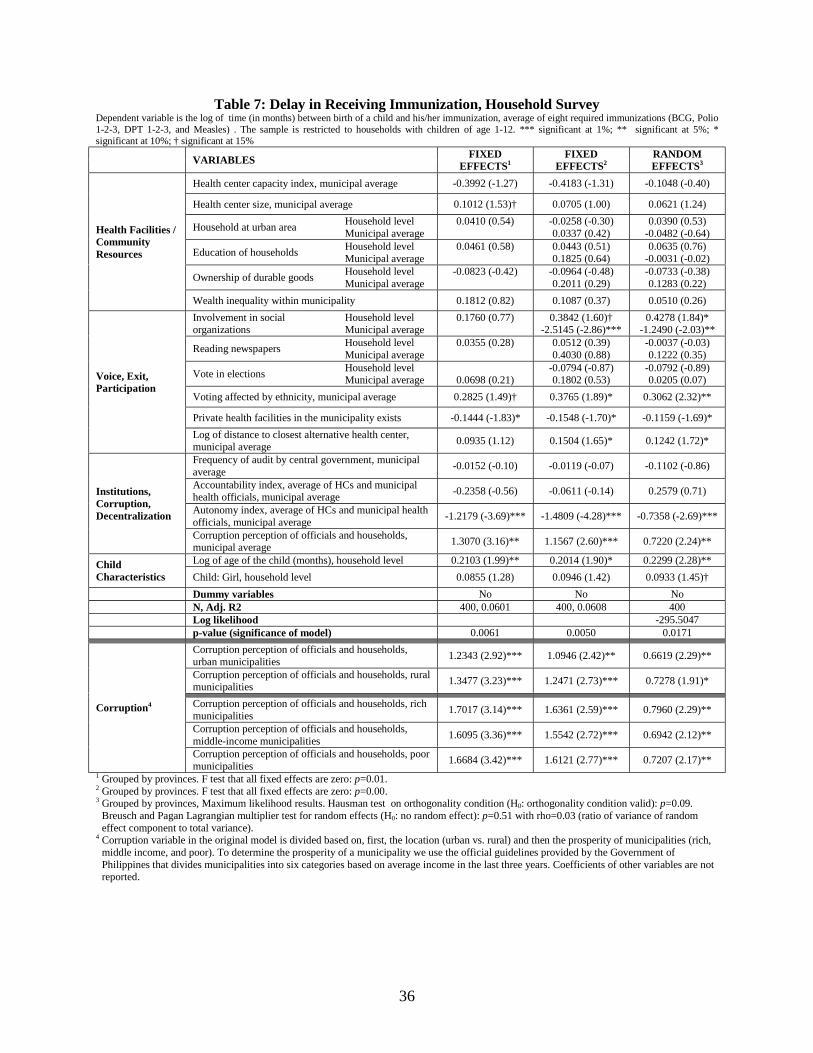
36

Table 7: Delay in Receiving Immunization, Household SurveyDependent variable is the log of time (in months) between birth of a child and his/her immunization, average of eight required immunizations (BCG, Polio1-2-3, DPT 1-2-3, and Measles) . The sample is restricted to households with children of age 1-12. *** significant at 1%; ** significant at 5%; *significant at 10%; † significant at 15%


FIXEDEFFECTS2

RANDOMEFFECTS3

Health center capacity index, municipal average -0.3992 (-1.27) -0.4183 (-1.31) -0.1048 (-0.40)

Health center size, municipal average 0.1012 (1.53)† 0.0705 (1.00) 0.0621 (1.24)


0.0410 (0.54) -0.0258 (-0.30)0.0337 (0.42)

0.0390 (0.53)-0.0482 (-0.64)


0.0461 (0.58) 0.0443 (0.51)0.1825 (0.64)

0.0635 (0.76)-0.0031 (-0.02)


-0.0823 (-0.42) -0.0964 (-0.48)0.2011 (0.29)

-0.0733 (-0.38)0.1283 (0.22)

Health Facilities /CommunityResources

Wealth inequality within municipality 0.1812 (0.82) 0.1087 (0.37) 0.0510 (0.26)Involvement in socialorganizations

Household levelMunicipal average

0.1760 (0.77) 0.3842 (1.60)†-2.5145 (-2.86)***

0.4278 (1.84)*-1.2490 (-2.03)**


0.0355 (0.28) 0.0512 (0.39)0.4030 (0.88)

-0.0037 (-0.03)0.1222 (0.35)

Vote in elections Household levelMunicipal average 0.0698 (0.21)

-0.0794 (-0.87)0.1802 (0.53)

-0.0792 (-0.89)0.0205 (0.07)

Voting affected by ethnicity, municipal average 0.2825 (1.49)† 0.3765 (1.89)* 0.3062 (2.32)**

Private health facilities in the municipality exists -0.1444 (-1.83)* -0.1548 (-1.70)* -0.1159 (-1.69)*


Log of distance to closest alternative health center,municipal average 0.0935 (1.12) 0.1504 (1.65)* 0.1242 (1.72)*

Frequency of audit by central government, municipalaverage -0.0152 (-0.10) -0.0119 (-0.07) -0.1102 (-0.86)

Accountability index, average of HCs and municipalhealth officials, municipal average -0.2358 (-0.56) -0.0611 (-0.14) 0.2579 (0.71)

Autonomy index, average of HCs and municipal healthofficials, municipal average -1.2179 (-3.69)*** -1.4809 (-4.28)*** -0.7358 (-2.69)***


Corruption perception of officials and households,municipal average 1.3070 (3.16)** 1.1567 (2.60)*** 0.7220 (2.24)**

Log of age of the child (months), household level 0.2103 (1.99)** 0.2014 (1.90)* 0.2299 (2.28)**ChildCharacteristics Child: Girl, household level 0.0855 (1.28) 0.0946 (1.42) 0.0933 (1.45)†

Dummy variables No No NoN, Adj. R2 400, 0.0601 400, 0.0608 400Log likelihood -295.5047p-value (significance of model) 0.0061 0.0050 0.0171Corruption perception of officials and households,urban municipalities 1.2343 (2.92)*** 1.0946 (2.42)** 0.6619 (2.29)**

Corruption perception of officials and households, ruralmunicipalities 1.3477 (3.23)*** 1.2471 (2.73)*** 0.7278 (1.91)*

Corruption perception of officials and households, richmunicipalities 1.7017 (3.14)*** 1.6361 (2.59)*** 0.7960 (2.29)**

Corruption perception of officials and households,middle-income municipalities 1.6095 (3.36)*** 1.5542 (2.72)*** 0.6942 (2.12)**

Corruption4

Corruption perception of officials and households, poormunicipalities 1.6684 (3.42)*** 1.6121 (2.77)*** 0.7207 (2.17)**

1 Grouped by provinces. F test that all fixed effects are zero: p=0.01.2 Grouped by provinces. F test that all fixed effects are zero: p=0.00.3 Grouped by provinces, Maximum likelihood results. Hausman test on orthogonality condition (H0: orthogonality condition valid): p=0.09.

Breusch and Pagan Lagrangian multiplier test for random effects (H0: no random effect): p=0.51 with rho=0.03 (ratio of variance of randomeffect component to total variance).

4 Corruption variable in the original model is divided based on, first, the location (urban vs. rural) and then the prosperity of municipalities (rich,middle income, and poor). To determine the prosperity of a municipality we use the official guidelines provided by the Government ofPhilippines that divides municipalities into six categories based on average income in the last three years. Coefficients of other variables are notreported.

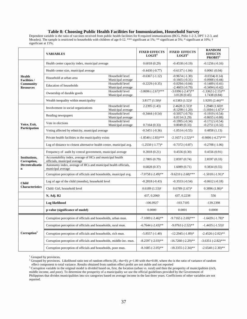
37

Table 8: Choosing Public Health Facilities for Immunization, Household SurveyDependent variable is the ratio of vaccines received from public health facilities for 8 required immunizations (BCG, Polio 1-2-3, DPT 1-2-3, andMeasles). The sample is restricted to households with children of age 0-12. *** significant at 1%; ** significant at 5%; * significant at 10%; †significant at 15%;


FIXED EFFECTSLOGIT1

RANDOMEFFECTSPROBIT2

Health center capacity index, municipal average 0.6018 (0.29) -0.4558 (-0.19) -0.1256 (-0.16)

Health center size, municipal average -0.4430 (-0.77) -0.6137 (-1.04) 0.0061 (0.04)


-0.6367 (-1.12) -0.9674 (-1.30)-0.1665 (-0.31)

-0.0334(-0.14)-0.0908 (-0.44)


-0.2229 (-0.35) -0.0294 (-0.04)-2.4603 (-0.79)

-0.1409 (-0.41)-0.3494 (-0.42)


-3.0696 (-2.67)*** -3.0396 (-2.47)**3.0128 (0.45)

-1.3362 (-2.15)**1.7438 (0.84)


Wealth inequality within municipality 3.8177 (1.50)† 4.5383 (1.52)† 1.9295 (2.44)**

Involvement in social organizations Household levelMunicipal average

2.2395 (1.43) 2.4628 (1.51)†-8.1298 (-1.20)

1.2948 (1.60)†-3.1694 (-1.67)*


-0.3444 (-0.54) -0.5057 (-0.76)6.0114 (1.29)

-0.1919 (-0.54)-0.8655 (-0.88)


-0.1995 (-0.34)0.8049 (0.33)

-0.1712 (-0.54)-0.2751 (-0.32)

Voting affected by ethnicity, municipal average -0.5451 (-0.36) -1.0514 (-0.55) 0.4858 (1.13)

Private health facilities in the municipality exists -1.8540 (-2.83)*** -2.1657 (-2.52)** -0.9006 (-4.27)***


Log of distance to closest alternative health center, municipal avg. -1.2550 (-1.77)* -0.7372 (-0.87) -0.2708 (-1.06)

Frequency of audit by central government, municipal average 0.2818 (0.21) 0.4556 (0.30) 0.4556 (0.91)

Accountability index, average of HCs and municipal healthofficials, municipal average 2.7805 (0.79) 2.8597 (0.74) 2.8597 (0.33)

Autonomy index, average of HCs and municipal health officials,municipal average 0.6828 (0.37) 1.6089 (0.71) 0.3834 (0.55)


Corruption perception of officials and households, municipal avg. -7.0758 (-2.49)** -9.6210 (-2.68)*** -1.5018 (-1.91)*

Log of age of the child (months), household level -0.2818 (-0.43) -0.3553 (-0.54) -0.0612 (-0.18)ChildCharacteristics Child: Girl, household level 0.6189 (1.53)† 0.6789 (1.67)* 0.3896 (1.86)*

N, Adj. R2 437, 0.2060 437, 0.2238 556

Log likelihood -106.0927 -103.7105 -139.2398

p-value (significance of model) 0.0000 0.0001 0.0000

Corruption perception of officials and households, urban mun. -7.1009 (-2.46)** -9.7165 (-2.69)*** -1.6439 (-1.78)*

Corruption perception of officials and households, rural mun. -6.7644 (-2.43)** -9.0763 (-2.52)** -1.4435 (-1.53)†

7 0758 ( 2 49)** 9 6210 ( 2 68)*** M i i l ACorruption perception of officials and households, rich mun. -5.8557 (-1.40) -12.2945 (-1.89)* -2.4526 (-2.02)**

Corruption perception of officials and households, middle-inc. mun. -8.2597 (-2.03)** -16.7260 (-2.29)** -3.6351 (-2.82)***

Corruption3

Corruption perception of officials and households, poor mun. -8.1685 (-2.05)** -18.3355 (-2.34)** -2.6540 (-2.30)**

1 Grouped by provinces.2 Grouped by provinces. Likelihood ratio test of random effects (Ho: rho=0): p=1.00 with rho=0.00, where rho is the ratio of variance of random

effect component to total variance. Results obtained from random effect probit are not stable and not reported3 Corruption variable in the original model is divided based on, first, the location (urban vs. rural) and then the prosperity of municipalities (rich,middle income, and poor). To determine the prosperity of a municipality we use the official guidelines provided by the Government ofPhilippines that divides municipalities into six categories based on average income in the last three years. Coefficients of other variables are notreported.

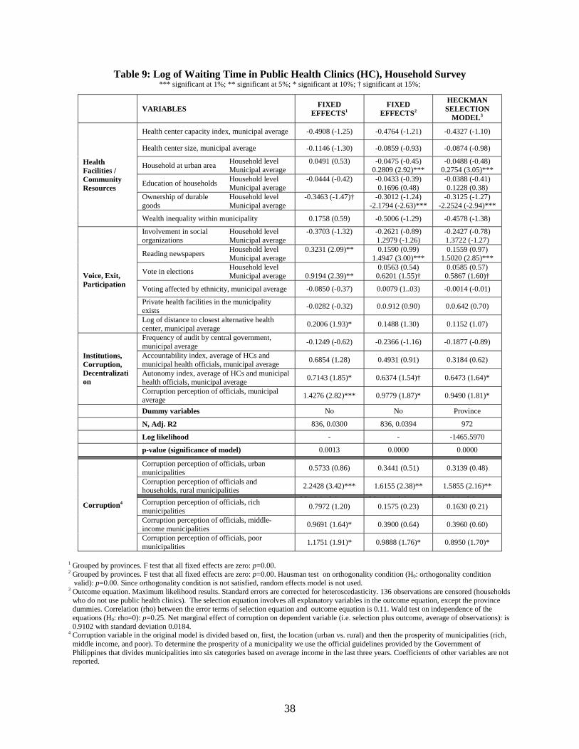
38

Table 9: Log of Waiting Time in Public Health Clinics (HC), Household Survey*** significant at 1%; ** significant at 5%; * significant at 10%; † significant at 15%;


FIXEDEFFECTS2

HECKMANSELECTION

MODEL3

Health center capacity index, municipal average -0.4908 (-1.25) -0.4764 (-1.21) -0.4327 (-1.10)

Health center size, municipal average -0.1146 (-1.30) -0.0859 (-0.93) -0.0874 (-0.98)


0.0491 (0.53) -0.0475 (-0.45)0.2809 (2.92)***

-0.0488 (-0.48)0.2754 (3.05)***


-0.0444 (-0.42) -0.0433 (-0.39)0.1696 (0.48)

-0.0388 (-0.41)0.1228 (0.38)

Ownership of durablegoods


-0.3463 (-1.47)† -0.3012 (-1.24)-2.1794 (-2.63)***

-0.3125 (-1.27)-2.2524 (-2.94)***


Wealth inequality within municipality 0.1758 (0.59) -0.5006 (-1.29) -0.4578 (-1.38)



-0.3703 (-1.32) -0.2621 (-0.89)1.2979 (-1.26)

-0.2427 (-0.78)1.3722 (-1.27)


0.3231 (2.09)** 0.1590 (0.99)1.4947 (3.00)***

0.1559 (0.97)1.5020 (2.85)***

Vote in elections Household levelMunicipal average 0.9194 (2.39)**

0.0563 (0.54)0.6201 (1.55)†

0.0585 (0.57)0.5867 (1.60)†

Voting affected by ethnicity, municipal average -0.0850 (-0.37) 0.0079 (1..03) -0.0014 (-0.01)

Private health facilities in the municipalityexists -0.0282 (-0.32) 0.0.912 (0.90) 0.0.642 (0.70)


Log of distance to closest alternative healthcenter, municipal average 0.2006 (1.93)* 0.1488 (1.30) 0.1152 (1.07)

Frequency of audit by central government,municipal average -0.1249 (-0.62) -0.2366 (-1.16) -0.1877 (-0.89)

Accountability index, average of HCs andmunicipal health officials, municipal average 0.6854 (1.28) 0.4931 (0.91) 0.3184 (0.62)

Autonomy index, average of HCs and municipalhealth officials, municipal average 0.7143 (1.85)* 0.6374 (1.54)† 0.6473 (1.64)*


Corruption perception of officials, municipalaverage 1.4276 (2.82)*** 0.9779 (1.87)* 0.9490 (1.81)*

Dummy variables No No Province

N, Adj. R2 836, 0.0300 836, 0.0394 972

Log likelihood - - -1465.5970

p-value (significance of model) 0.0013 0.0000 0.0000

Corruption perception of officials, urbanmunicipalities 0.5733 (0.86) 0.3441 (0.51) 0.3139 (0.48)

Corruption perception of officials andhouseholds, rural municipalities 2.2428 (3.42)*** 1.6155 (2.38)** 1.5855 (2.16)**

M i i l A M i i l A M i i l ACorruption perception of officials, richmunicipalities 0.7972 (1.20) 0.1575 (0.23) 0.1630 (0.21)

Corruption perception of officials, middle-income municipalities 0.9691 (1.64)* 0.3900 (0.64) 0.3960 (0.60)

Corruption4

Corruption perception of officials, poormunicipalities 1.1751 (1.91)* 0.9888 (1.76)* 0.8950 (1.70)*

1 Grouped by provinces. F test that all fixed effects are zero: p=0.00.2 Grouped by provinces. F test that all fixed effects are zero: p=0.00. Hausman test on orthogonality condition (H0: orthogonality condition

valid): p=0.00. Since orthogonality condition is not satisfied, random effects model is not used.3 Outcome equation. Maximum likelihood results. Standard errors are corrected for heteroscedasticity. 136 observations are censored (households

who do not use public health clinics). The selection equation involves all explanatory variables in the outcome equation, except the provincedummies. Correlation (rho) between the error terms of selection equation and outcome equation is 0.11. Wald test on independence of theequations (H0: rho=0): p=0.25. Net marginal effect of corruption on dependent variable (i.e. selection plus outcome, average of observations): is0.9102 with standard deviation 0.0184.


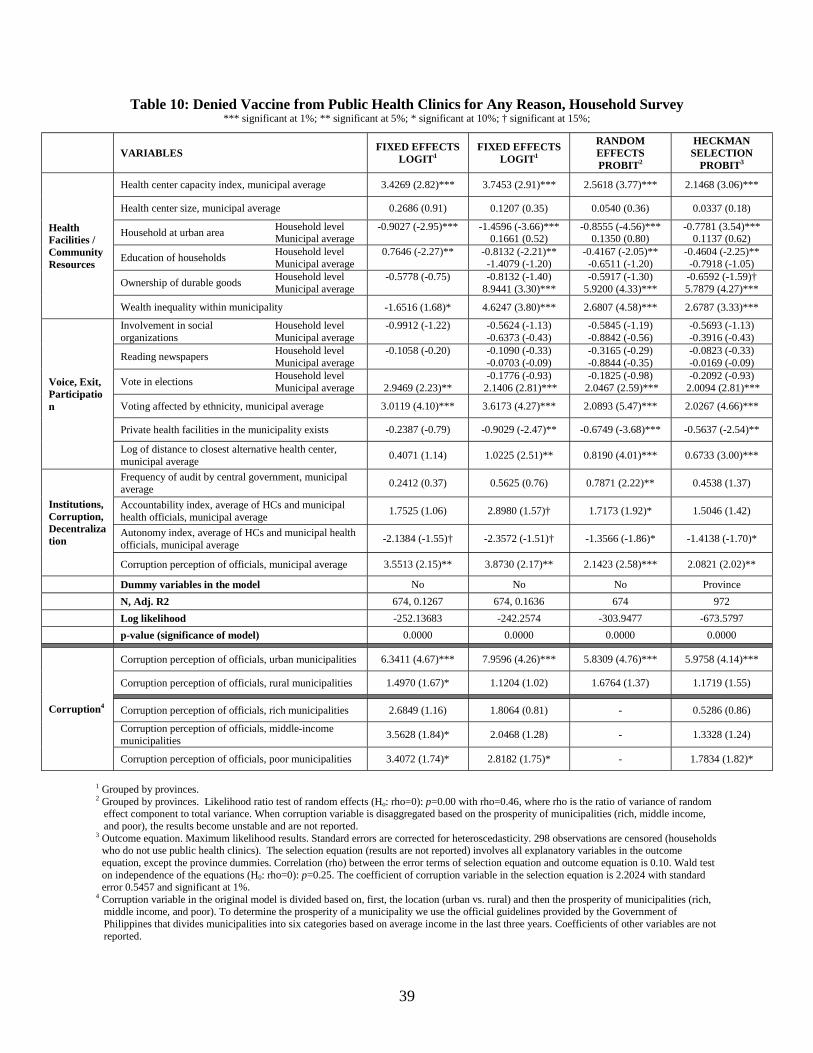
39

Table 10: Denied Vaccine from Public Health Clinics for Any Reason, Household Survey*** significant at 1%; ** significant at 5%; * significant at 10%; † significant at 15%;


FIXED EFFECTSLOGIT1


HECKMANSELECTION

PROBIT3

Health center capacity index, municipal average 3.4269 (2.82)*** 3.7453 (2.91)*** 2.5618 (3.77)*** 2.1468 (3.06)***

Health center size, municipal average 0.2686 (0.91) 0.1207 (0.35) 0.0540 (0.36) 0.0337 (0.18)


-0.9027 (-2.95)*** -1.4596 (-3.66)***0.1661 (0.52)

-0.8555 (-4.56)***0.1350 (0.80)

-0.7781 (3.54)***0.1137 (0.62)


0.7646 (-2.27)** -0.8132 (-2.21)**-1.4079 (-1.20)

-0.4167 (-2.05)**-0.6511 (-1.20)

-0.4604 (-2.25)**-0.7918 (-1.05)


-0.5778 (-0.75) -0.8132 (-1.40)8.9441 (3.30)***

-0.5917 (-1.30)5.9200 (4.33)***

-0.6592 (-1.59)†5.7879 (4.27)***


Wealth inequality within municipality -1.6516 (1.68)* 4.6247 (3.80)*** 2.6807 (4.58)*** 2.6787 (3.33)***



-0.9912 (-1.22) -0.5624 (-1.13)-0.6373 (-0.43)

-0.5845 (-1.19)-0.8842 (-0.56)

-0.5693 (-1.13)-0.3916 (-0.43)


-0.1058 (-0.20) -0.1090 (-0.33)-0.0703 (-0.09)

-0.3165 (-0.29)-0.8844 (-0.35)

-0.0823 (-0.33)-0.0169 (-0.09)

Vote in elections Household levelMunicipal average 2.9469 (2.23)**

-0.1776 (-0.93) 2.1406 (2.81)***

-0.1825 (-0.98) 2.0467 (2.59)***

-0.2092 (-0.93) 2.0094 (2.81)***

Voting affected by ethnicity, municipal average 3.0119 (4.10)*** 3.6173 (4.27)*** 2.0893 (5.47)*** 2.0267 (4.66)***

Private health facilities in the municipality exists -0.2387 (-0.79) -0.9029 (-2.47)** -0.6749 (-3.68)*** -0.5637 (-2.54)**


Log of distance to closest alternative health center,municipal average 0.4071 (1.14) 1.0225 (2.51)** 0.8190 (4.01)*** 0.6733 (3.00)***

Frequency of audit by central government, municipalaverage 0.2412 (0.37) 0.5625 (0.76) 0.7871 (2.22)** 0.4538 (1.37)

Accountability index, average of HCs and municipalhealth officials, municipal average 1.7525 (1.06) 2.8980 (1.57)† 1.7173 (1.92)* 1.5046 (1.42)

Autonomy index, average of HCs and municipal healthofficials, municipal average -2.1384 (-1.55)† -2.3572 (-1.51)† -1.3566 (-1.86)* -1.4138 (-1.70)*


Corruption perception of officials, municipal average 3.5513 (2.15)** 3.8730 (2.17)** 2.1423 (2.58)*** 2.0821 (2.02)**

Dummy variables in the model No No No ProvinceN, Adj. R2 674, 0.1267 674, 0.1636 674 972Log likelihood -252.13683 -242.2574 -303.9477 -673.5797p-value (significance of model) 0.0000 0.0000 0.0000 0.0000

Corruption perception of officials, urban municipalities 6.3411 (4.67)*** 7.9596 (4.26)*** 5.8309 (4.76)*** 5.9758 (4.14)***

Corruption perception of officials, rural municipalities 1.4970 (1.67)* 1.1204 (1.02) 1.6764 (1.37) 1.1719 (1.55)

Corruption perception of officials, rich municipalities 2.6849 (1.16) 1.8064 (0.81) - 0.5286 (0.86)

Corruption perception of officials, middle-incomemunicipalities 3.5628 (1.84)* 2.0468 (1.28) - 1.3328 (1.24)

Corruption4

Corruption perception of officials, poor municipalities 3.4072 (1.74)* 2.8182 (1.75)* - 1.7834 (1.82)*


effect component to total variance. When corruption variable is disaggregated based on the prosperity of municipalities (rich, middle income,and poor), the results become unstable and are not reported.

3 Outcome equation. Maximum likelihood results. Standard errors are corrected for heteroscedasticity. 298 observations are censored (householdswho do not use public health clinics). The selection equation (results are not reported) involves all explanatory variables in the outcomeequation, except the province dummies. Correlation (rho) between the error terms of selection equation and outcome equation is 0.10. Wald teston independence of the equations (H0: rho=0): p=0.25. The coefficient of corruption variable in the selection equation is 2.2024 with standarderror 0.5457 and significant at 1%.


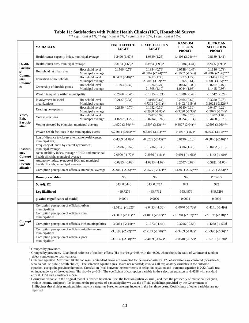
40

Table 11: Satisfaction with Public Health Clinics (HC), Household Survey*** significant at 1%; ** significant at 5%; * significant at 10%; † significant at 15%;


FIXED EFFECTSLOGIT1


HECKMANSELECTION

PROBIT4

Health center capacity index, municipal average 1.2490 (1.47)† 1.0839 (1.25) 1.4103 (3.24)*** 0.8189 (1.41)

Health center size, municipal average 0.3153 (1.65)* 0.3964 (1.93)* -0.1088 (-1.41) 0.2425 (1.91)*


0.1560 (0.79) 0.1854 (0.76)-0.5862 (-2.74)***

-0.0558 (-0.47)-0.1687 (-1.54)†

0.1146 (0.78)-0.2882 (-2.96)***


0.5403 (2.40)** 0.3217 (1.35)2.9808 (3.62)***

0.1777 (1.22)0.1892 (0.61)

0.2146 (1.47) †1.9088 (3.95)***


0.1893 (0.37) 0.1326 (0.24)2.1308 (1.10)

-0.0166 (-0.05)1.0044 (1.06)

0.0267 (0.07)1.1415 (0.95)

HealthFacilities/CommunityResources

Wealth inequality within municipality -0.2960 (-0.45) -0.1815 (-0.21) -0.1388 (-0.43) -0.1542 (-0.29)



0.2127 (0.34) 0.4198 (0.64)-4.7302 (-2.01)**

0.2664 (0.67)-1.4402 (-1.54)†

0.3250 (0.78)-3.1022 (-2.22)**


-0.2350 (-0.70) 0.1052 (0.30)-2.2968 (-1.85)*

0.0640 (0.30)-0.9290 (-1.93)*

0.0497 (0.22)-1.3075 (-1.74)*

Vote in elections Household levelMunicipal average -1.0297 (-1.22)

0.2207 (0.97)-0.8234 (-0.92)

0.1026 (0.75)-0.0624 (-0.14)

0.1482 (1.04)-0.4458 (-0.79)

Voting affected by ethnicity, municipal average 1.4920 (2.84)*** 1.6507 (3.13)*** 0.3827 (2.04)** 1.0505 (3.26)***

Private health facilities in the municipality exists 0.78041 (3.94)*** 0.8309 (3.51)*** 0.1957 (1.87)* 0.5039 (3.51)***

Voice,Exit,Participation

Log of distance to closest alternative health center,municipal avg. -0.4339 (-1.89)* -0.6265 (-2.43)** 0.0190 (0.16) -0.3840 (-2.46)**

Frequency of audit by central government,municipal average -0.2686 (-0.57) -0.1736 (-0.35) 0.3086 (1.38) -0.0462 (-0.15)

Accountability index, average of HCs and municipalhealth officials, municipal average -2.0900 (-1.77)* -2.2966 (-1.81)* -0.9914 (-1.66)* -1.4142 (-1.90)*

Autonomy index, average of HCs and municipalhealth officials, municipal average -0.0215 (-0.03) -1.0253 (-1.09) 0.2507 (0.69) -0.5921 (-1.00)

Institutions,Corruption,Decentralization Corruption perception of officials, municipal average -2.0900 (-2.56)*** -2.5575 (-2.17)** -1.4285 (-2.95)*** -1.7126 (-2.33)**

Dummy variables No No No Province

N, Adj. R2 843, 0.0448 843, 0.0714 843 972

Log likelihood -499.7276 -485.7732 -555.4976 -849.5293


Corruption perception of officials, urbanmunicipalities -2.6112 (-1.82)* -2.0433 (-1.36) -1.0670 (-1.73)* -1.4141 (-1.49)†

Corruption perception of officials, ruralmunicipalities -3.0092 (-2.11)** -3.1031 (-2.02)** -1.9284 (-2.67)*** -2.0189 (-2.18)**

Corruption perception of officials, rich municipalities -3.0881 (-2.14)** -2.1973 (-1.44) -0.3206 (-0.55) -1.4268 (-1.53)†

Corruption perception of officials, middle-incomemunicipalities -3.5193 (-2.72)*** -2.7149 (-1.98)** -0.9489 (-1.82)* -1.7398 (-2.06)**

Corruption4

Corruption perception of officials, poormunicipalities -3.6137 (-2.68)*** -2.4069 (-1.67)* -0.8510 (-1.72)* -1.5731 (-1.78)*


effect component to total variance.3 Outcome equation. Maximum likelihood results. Standard errors are corrected for heteroscedasticity. 129 observations are censored (households

who do not use public health clinics). The selection equation (results are not reported) involves all explanatory variables in the outcomeequation, except the province dummies. Correlation (rho) between the error terms of selection equation and outcome equation is 0.22. Wald teston independence of the equations (H0: rho=0): p=0.24. The coefficient of corruption variable in the selection equation is -1.4538 with standarderror 0..4161 and significant at 5%.


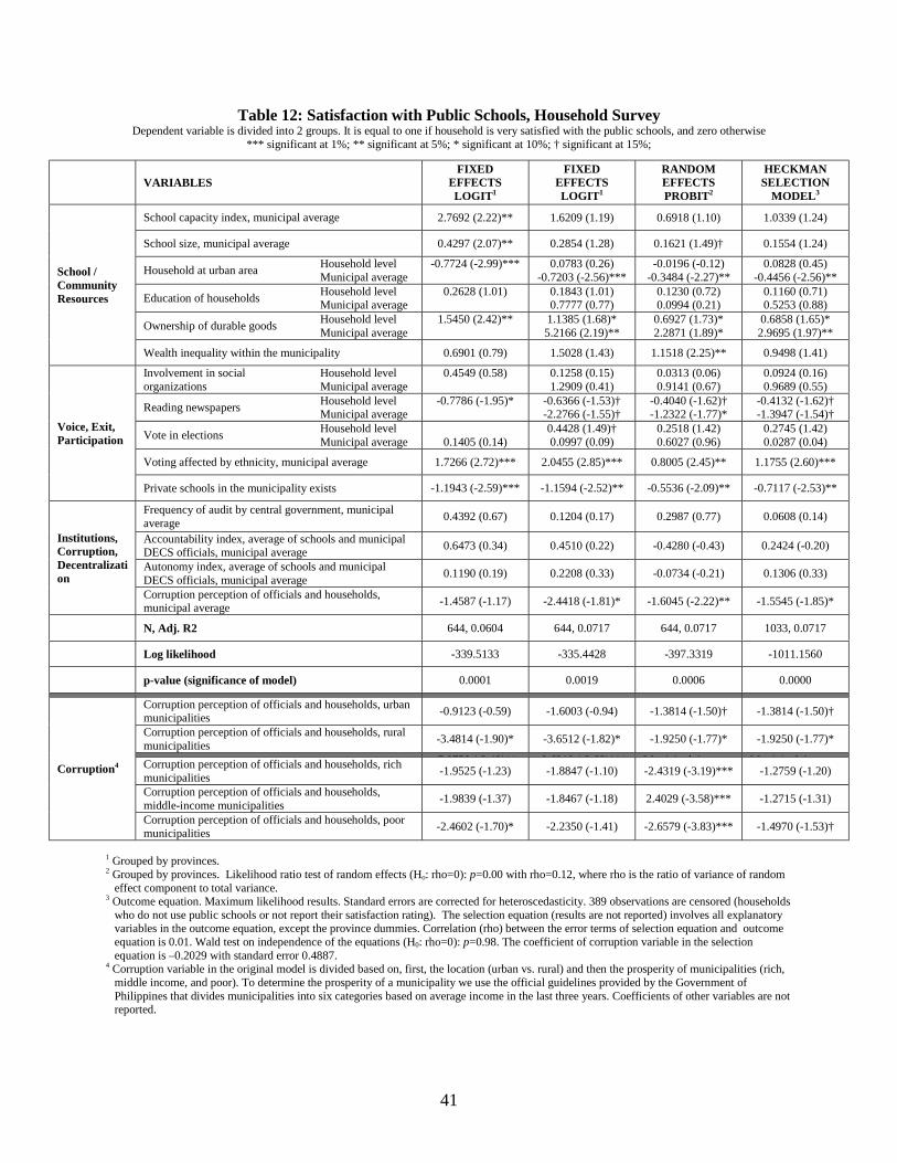
41

Table 12: Satisfaction with Public Schools, Household SurveyDependent variable is divided into 2 groups. It is equal to one if household is very satisfied with the public schools, and zero otherwise

*** significant at 1%; ** significant at 5%; * significant at 10%; † significant at 15%;

VARIABLESFIXED

EFFECTSLOGIT1

FIXEDEFFECTSLOGIT1


HECKMANSELECTION

MODEL3

School capacity index, municipal average 2.7692 (2.22)** 1.6209 (1.19) 0.6918 (1.10) 1.0339 (1.24)

School size, municipal average 0.4297 (2.07)** 0.2854 (1.28) 0.1621 (1.49)† 0.1554 (1.24)


-0.7724 (-2.99)*** 0.0783 (0.26)-0.7203 (-2.56)***

-0.0196 (-0.12)-0.3484 (-2.27)**

0.0828 (0.45)-0.4456 (-2.56)**


0.2628 (1.01) 0.1843 (1.01)0.7777 (0.77)

0.1230 (0.72)0.0994 (0.21)

0.1160 (0.71)0.5253 (0.88)


1.5450 (2.42)** 1.1385 (1.68)*5.2166 (2.19)**

0.6927 (1.73)*2.2871 (1.89)*

0.6858 (1.65)*2.9695 (1.97)**

School /CommunityResources

Wealth inequality within the municipality 0.6901 (0.79) 1.5028 (1.43) 1.1518 (2.25)** 0.9498 (1.41)



0.4549 (0.58) 0.1258 (0.15)1.2909 (0.41)

0.0313 (0.06)0.9141 (0.67)

0.0924 (0.16)0.9689 (0.55)


-0.7786 (-1.95)* -0.6366 (-1.53)†-2.2766 (-1.55)†

-0.4040 (-1.62)†-1.2322 (-1.77)*

-0.4132 (-1.62)†-1.3947 (-1.54)†


0.4428 (1.49)†0.0997 (0.09)

0.2518 (1.42)0.6027 (0.96)

0.2745 (1.42)0.0287 (0.04)

Voting affected by ethnicity, municipal average 1.7266 (2.72)*** 2.0455 (2.85)*** 0.8005 (2.45)** 1.1755 (2.60)***


Private schools in the municipality exists -1.1943 (-2.59)*** -1.1594 (-2.52)** -0.5536 (-2.09)** -0.7117 (-2.53)**

Frequency of audit by central government, municipalaverage 0.4392 (0.67) 0.1204 (0.17) 0.2987 (0.77) 0.0608 (0.14)

Accountability index, average of schools and municipalDECS officials, municipal average 0.6473 (0.34) 0.4510 (0.22) -0.4280 (-0.43) 0.2424 (-0.20)

Autonomy index, average of schools and municipalDECS officials, municipal average 0.1190 (0.19) 0.2208 (0.33) -0.0734 (-0.21) 0.1306 (0.33)


Corruption perception of officials and households,municipal average -1.4587 (-1.17) -2.4418 (-1.81)* -1.6045 (-2.22)** -1.5545 (-1.85)*

N, Adj. R2 644, 0.0604 644, 0.0717 644, 0.0717 1033, 0.0717

Log likelihood -339.5133 -335.4428 -397.3319 -1011.1560


Corruption perception of officials and households, urbanmunicipalities -0.9123 (-0.59) -1.6003 (-0.94) -1.3814 (-1.50)† -1.3814 (-1.50)†

Corruption perception of officials and households, ruralmunicipalities -3.4814 (-1.90)* -3.6512 (-1.82)* -1.9250 (-1.77)* -1.9250 (-1.77)*

7 0758 ( 2 49)** 9 6210 ( 2 68)*** M i i l A M i i l ACorruption perception of officials and households, richmunicipalities -1.9525 (-1.23) -1.8847 (-1.10) -2.4319 (-3.19)*** -1.2759 (-1.20)

Corruption perception of officials and households,middle-income municipalities -1.9839 (-1.37) -1.8467 (-1.18) 2.4029 (-3.58)*** -1.2715 (-1.31)

Corruption4

Corruption perception of officials and households, poormunicipalities -2.4602 (-1.70)* -2.2350 (-1.41) -2.6579 (-3.83)*** -1.4970 (-1.53)†


effect component to total variance.3 Outcome equation. Maximum likelihood results. Standard errors are corrected for heteroscedasticity. 389 observations are censored (households

who do not use public schools or not report their satisfaction rating). The selection equation (results are not reported) involves all explanatoryvariables in the outcome equation, except the province dummies. Correlation (rho) between the error terms of selection equation and outcomeequation is 0.01. Wald test on independence of the equations (H0: rho=0): p=0.98. The coefficient of corruption variable in the selectionequation is –0.2029 with standard error 0.4887.


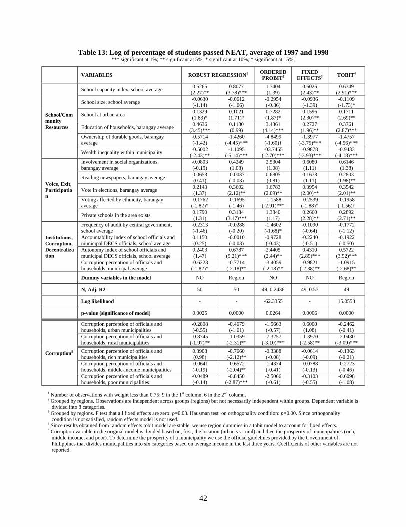
42

Table 13: Log of percentage of students passed NEAT, average of 1997 and 1998*** significant at 1%; ** significant at 5%; * significant at 10%; † significant at 15%;

VARIABLES ROBUST REGRESSION1 ORDEREDPROBIT2

FIXEDEFFECTS3 TOBIT4

School capacity index, school average 0.5265(2.27)**

0.8077(3.78)***

1.7404(1.39)

0.6025(2.43)**

0.6349(2.91)***

School size, school average -0.0630(-1.14)

-0.0612(-1.06)

-0.2954(-0.86)

-0.0936(-1.39)

-0.1109(-1.73)*

School at urban area 0.1329(1.83)*

0.1021(1.71)*

0.7282(1.87)*

0.1596(2.30)**

0.1711(2.69)**

Education of households, barangay average 0.4636(3.45)***

0.1180(0.99)

3.4361(4.14)***

0.2727(1.96)**

0.3761(2.87)***

Ownership of durable goods, barangayaverage

-0.5714(-1.42)

-1.4260(-4.45)***

-4.8499(-1.60)†

-1.3977(-3.75)***

-1.4757(-4.56)***

School/CommunityResources

Wealth inequality within municipality -0.5002(-2.43)**

-1.1095(-5.14)***

-03.7455(-2.70)***

-0.9878(-3.93)***

-0.9433(-4.18)***

Involvement in social organizations,barangay average

-0.0803(-0.19)

0.4249(1.08)

2.5304(1.08)

0.6080(1.11)

0.6146(1.38)

Reading newspapers, barangay average 0.0653(0.41)

-0.0037(-0.03)

0.6805(0.81)

0.1673(1.11)

0.2803(1.98)**

Vote in elections, barangay average 0.2143(1.37)

0.3602(2.12)**

1.6783(2.09)**

0.3954(2.00)**

0.3542(2.01)**

Voting affected by ethnicity, barangayaverage

-0.1762(-1.82)*

-0.1695(-1.46)

-1.1588(-2.91)***

-0.2539(-1.88)*

-0.1958(-1.56)†


Private schools in the area exists 0.1790(1.31)

0.3184(3.17)***

1.3840(1.17)

0.2660(2.28)**

0.2892(2.71)**

Frequency of audit by central government,school average

-0.2313(-1.46)

-0.0288(-0.20)

-1.4602(-1.68)*

-0.1090(-0.64)

-0.1772(-1.12)

Accountability index of school officials andmunicipal DECS officials, school average

0.1150(0.25)

-0.0010(-0.03)

-0.9728(-0.43)

-0.2240(-0.51)

-0.1922(-0.50)

Autonomy index of school officials andmunicipal DECS officials, school average

0.2403(1.47)

0.6787(5.21)***

2.4405(2.44)**

0.4310(2.85)***

0.5722(3.92)***



-0.6223(-1.82)*

-0.7714(-2.18)**

-3.4059(-2.18)**

-0.9821(-2.38)**

-1.0915(-2.68)**

Dummy variables in the model NO Region NO NO Region

N, Adj. R2 50 50 49, 0.2436 49, 0.57 49

Log likelihood - - -62.3355 - 15.0553

p-value (significance of model) 0.0025 0.0000 0.0264 0.0006 0.0000


-0.2808(-0.55)

-0.4679(-1.01)

-1.5663(-0.57)

0.6000(1.08)

-0.2462(-0.41)


-0.8745(-1.97)**

-1.0359(-2.31)**

-7.3257(-3.10)***

-1.3970(-2.58)**

-2.0430(-3.09)***


0.3908(0.98)

-0.7660(-2.12)**

-0.3388(-0.08)

-0.0614(-0.09)

-0.1363(-0.21)


-0.0641(-0.19)

-0.6572(-2.04)**

-1.4374(-0.41)

-0.0788(-0.13)

-0.2723(-0.46)

Corruption5


-0.0489(-0.14)

-0.8450(-2.87)***

-2.5066(-0.61)

-0.3103(-0.55)

-0.6098(-1.08)

1 Number of observations with weight less than 0.75: 9 in the 1st column, 6 in the 2nd column.2 Grouped by regions. Observations are independent across groups (regions) but not necessarily independent within groups. Dependent variable is

divided into 8 categories.3 Grouped by regions. F test that all fixed effects are zero: p=0.03. Hausman test on orthogonality condition: p=0.00. Since orthogonality

condition is not satisfied, random effects model is not used.4 Since results obtained from random effects tobit model are stable, we use region dummies in a tobit model to account for fixed effects.5 Corruption variable in the original model is divided based on, first, the location (urban vs. rural) and then the prosperity of municipalities (rich,


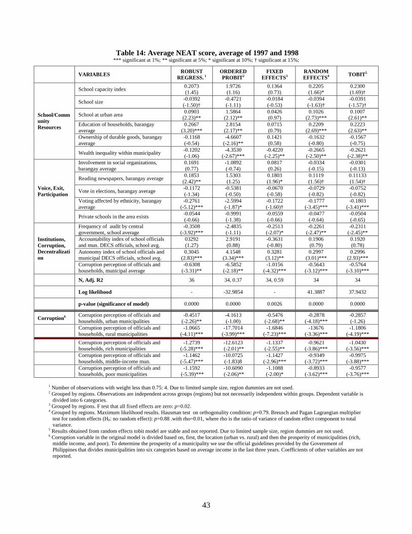
43

Table 14: Average NEAT score, average of 1997 and 1998*** significant at 1%; ** significant at 5%; * significant at 10%; † significant at 15%;

VARIABLES ROBUSTREGRESS. 1

ORDEREDPROBIT2

FIXEDEFFECTS3

RANDOMEFFECTS4 TOBIT5

School capacity index 0.2073(1.45)

1.9726(1.16)

0.1364(0.73)

0.2205(1.66)*

0.2300(1.69)†

School size -0.0392(-1.50)†

-0.4721(-1.11)

-0.0184(-0.53)

-0.0394(-1.63)†

-0.0391(-1.57)†

School at urban area 0.0903(2.23)**

1.5864(2.12)**

0.0426(0.97)

0.1026(2.73)***

0.1007(2.61)**

Education of households, barangayaverage

0.2667(3.20)***

2.8154(2.17)**

0.0715(0.79)

0.2209(2.69)***

0.2223(2.63)**


-0.1168(-0.54)

-4.6607(-2.16)**

0.1421(0.58)

-0.1632(-0.80)

-0.1567(-0.75)



-4.3530(-2.67)***

-0.4220(-2.25)**

-0.2665(-2.50)**

-0.2621(-2.38)**

Involvement in social organizations,barangay average

0.1691(0.77)

-1.0892(-0.74)

0.0817(0.26)

-0.0334(-0.15)

-0.0301(-0.13)

Reading newspapers, barangay average 0.1853(2.42)**

1.5303(1.25)

0.1803(1.96)*

0.1119(1.56)†

0.11133(1.54)†

Vote in elections, barangay average -0.1172(-1.34)

-0.5381(-0.50)

-0.0670(-0.58)

-0.0729(-0.82)

-0.0752(-0.82)


-0.2761(-5.12)***

-2.5994(-1.87)*

-0.1722(-1.60)†

-0.1777(-3.45)***

-0.1803(-3.41)***


Private schools in the area exists -0.0544(-0.66)

-0.9991(-1.38)

-0.0559(-0.66)

-0.0477(-0.64)

-0.0504(-0.65)

Frequency of audit by centralgovernment, school average

-0.3508(-3.92)***

-2.4835(-1.11)

-0.2513(-2.07)*

-0.2261(-2.47)**

-0.2311(-2.45)**

Accountability index of school officialsand mun. DECS officials, school avg.

03292(1.27)

2.9191(0.88)

-0.3631(-0.80)

0.1906(0.79)

0.1920(0.78)

Autonomy index of school officials andmunicipal DECS officials, school avg.

0.3045(2.83)***

4.1548(3.34)***

0.3281(3.12)**

0.2997(3.01)***

0.2996(2.93)***



-0.6308(-3.31)**

-6.5852(-2.18)**

-1.0156(-4.32)***

-0.5643(-3.12)***

-0.5764(-3.10)***

N, Adj. R2 36 34, 0.37 34, 0.59 34 34

Log likelihood - -32.9854 - 41.3887 37.9432

p-value (significance of model) 0.0000 0.0000 0.0026 0.0000 0.0000

Corruption6 Corruption perception of officials andhouseholds, urban municipalities

-0.4517(-2.26)**

-4.1613(-1.00)

-0.5476(-2.68)**

-0.2878(-4.18)***

-0.2857(-1.26)


-1.0665(-4.11)***

-17.7014(-3.99)***

-1.6846(-7.23)***

-13676(-3.36)***

-1.1806(-4.19)***


-1.2739(-5.28)***

-12.6123 (-2.01)**

-1.1337(-2.55)**

-0.9621(-3.86)***

-1.0430(-3.56)***

Corruption perception of officials andhouseholds, middle-income mun.

-1.1462(-5.47)***

-10.0725(-1.83)8

-1.1427(-2.96)***

-0.9349(-3.72)***

-0.9975(-3.88)***


-1.1592 (-5.39)***

-10.6090 (-2.06)**

-1.1088(-2.00)*

-0.8933(-3.62)***

-0.9577(-3.76)***

1 Number of observations with weight less than 0.75: 4. Due to limited sample size, region dummies are not used.2 Grouped by regions. Observations are independent across groups (regions) but not necessarily independent within groups. Dependent variable is

divided into 6 categories.3 Grouped by regions. F test that all fixed effects are zero: p=0.02.4 Grouped by regions. Maximum likelihood results. Hausman test on orthogonality condition: p=0.79. Breusch and Pagan Lagrangian multiplier

test for random effects (H0: no random effect): p=0.88 .with rho=0.01, where rho is the ratio of variance of random effect component to totalvariance.

5 Results obtained from random effects tobit model are stable and not reported. Due to limited sample size, region dummies are not used.6 Corruption variable in the original model is divided based on, first, the location (urban vs. rural) and then the prosperity of municipalities (rich,


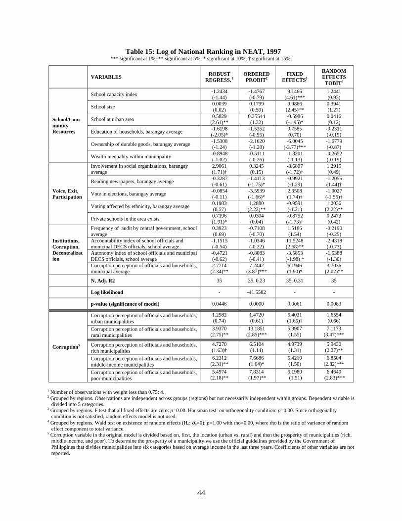
44

Table 15: Log of National Ranking in NEAT, 1997*** significant at 1%; ** significant at 5%; * significant at 10%; † significant at 15%;


ORDEREDPROBIT2

FIXEDEFFECTS3

RANDOMEFFECTS

TOBIT4

School capacity index -1.2434(-1.44)

-1.4767(-0.79)

9.1466(4.61)***

1.2441(0.93)

School size 0.0039(0.02)

0.1799(0.59)

0.9866(2.45)**

0.3941(1.27)

School at urban area 0.5829(2.61)**

0.35544(1.32)

-0.5986(-1.95)*

0.0416(0.12)

Education of households, barangay average -1.6198(-2.05)*

-1.5352(-0.95)

0.7585(0.70)

-0.2311(-0.19)

Ownership of durable goods, barangay average -1.5308(-1.24)

-2.1620(-1.28)

-6.0045(-3.77)***

-1.6779(-0.87)



-0.5111(-0.26)

-1.8201(-1.13)

-0.2652(-0.19)

Involvement in social organizations, barangayaverage

2.9061(1.71)†

0.3245(0.15)

-8.6807(-1.72)†

1.2915(0.49)

Reading newspapers, barangay average -0.3287(-0.61)

-1.4113(-1.75)*

-0.9921(-1.29)

-1.2055(1.44)†


-3.5939(-1.66)*

2.3508(1.74)†

-1.9027(-1.56)†

Voting affected by ethnicity, barangay average 0.1983(0.57)

1.2880(2.22)**

-0.9591(-1.21)

1.2036(2.22)**


Private schools in the area exists 0.7196(1.91)*

0.0304(0.04)

-0.8752(-1.73)†

0.2473(0.42)

Frequency of audit by central government, schoolaverage

0.3923(0.69)

-0.7108(-0.70)

1.5186(1.54)

-0.2190(-0.25)


-1.1515(-0.54)

-1.0346(-0.22)

11.5248(2.68)**

-2.4318(-0.73)

Autonomy index of school officials and municipalDECS officials, school average

-0.4721(-0.62)

-0.8083(-0.41)

-3.5853(-1.98) *

-1.5388(-1.30)


Corruption perception of officials and households,municipal average

2.7714(2.34)**

7.2442(3.87)***

6.1946(1.90)*

3.7036(2.02)**

N, Adj. R2 35 35, 0.23 35, 0.31 35

Log likelihood - -41.5582 - -


Corruption perception of officials and households,urban municipalities

1.2982(0.74)

1.4720(0.61)

6.4031(1.65)†

1.6554(0.66)

Corruption perception of officials and households,rural municipalities

3.9370(2.75)**

13.1851(2.85)***

5.9907(1.55)

7.1173(3.47)***

Corruption perception of officials and households,rich municipalities

4.7270(1.63)†

6.5104(1.14)

4.9739(1.31)

5.9430(2.27)**

Corruption perception of officials and households,middle-income municipalities

6.2312(2.31)**

7.6686(1.64)*

5.4210(1.50)

6.8504(2.82)***

Corruption5

Corruption perception of officials and households,poor municipalities

5.4974(2.18)**

7.8314 (1.97)**

5.1980 (1.51)

6.4640 (2.83)***

1 Number of observations with weight less than 0.75: 4.2 Grouped by regions. Observations are independent across groups (regions) but not necessarily independent within groups. Dependent variable is

divided into 5 categories.3 Grouped by regions. F test that all fixed effects are zero: p=0.00. Hausman test on orthogonality condition: p=0.00. Since orthogonality

condition is not satisfied, random effects model is not used.4 Grouped by regions. Wald test on existence of random effects (Ho: σu=0): p=1.00 with rho=0.00, where rho is the ratio of variance of random

effect component to total variance.5 Corruption variable in the original model is divided based on, first, the location (urban vs. rural) and then the prosperity of municipalities (rich,


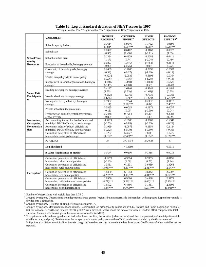
45

Table 16: Log of standard deviation of NEAT scores in 1997*** significant at 1%; ** significant at 5%; * significant at 10%; † significant at 15%;


ORDEREDPROBIT2

FIXEDEFFECTS3

RANDOMEFFECTS4

School capacity index 0.7614(1.82*

5.9546(3.00)***

1.1762(1.98)*

1.0190(3.28)***

School size 0.0327(0.35)

0.6462(1.49)†

-0.0167(-0.11)

0.0927(1.35)

School at urban area 0.1324(1.17)

0.4129(0.74)

-0.0288(-0.24)

0.0411(0.49)

Education of households, barangay average 0.0227(0.06)

-0.4464(-0.25)

0.4038(0.98)

0.2118(0.72)


0.2489(0.38)

-0.7805(-0.27)

-0.7995(-1.09)

-0.0936(-0.19)



-2.0533(-1.54)†

-0.6193(-1.28)

-0.0394(-0.13)

Involvement in social organizations, barangayaverage

-0.1485(-0.17)

-0.1981(-0.08)

1.0868(0.63)

-0.2524(-0.40)

Reading newspapers, barangay average 0.4127(1.55)†

1.6440(1.53)†

-0.4943(-1.66)†

0.1485(0.75)


-3.0166(-1.71)*

-0.7330(-1.67)†

-0.7366(-2.47)**


0.1902(1.11)

1.7844(2.96)***

0.2332(0.84)

0.3117(2.45)**



0.0015(0.00)

-0.0874(-0.39)

0.0057(0.04)

Frequency of audit by central government,school average

0.2448(0.86)

0.7984(0.83)

0.5364(1.48)

0.2088(1.99)


-0.5729(-0.53)

-3.3980(-0.83)

-0.0608(-0.05)

-0.2340(-0.29)

Autonomy index of school officials andmunicipal DECS officials, school average

0.1969(-0.52)

-1.0878(-0.79)

-0.1854(-0.50)

-0.1114(-0.39)



1.1222(1.83)*

5.4077(2.48)**

1.8111(1.95)*

1.1776(2.59)***

N, Adj. R2 37 37, 0.34 37, 0.28 37

Log likelihood - -41.3599 - 6.5311



-0.1278(-0.23)

4.3814(1.06)

0.7853(0.78)

0.8196(1.24)


1.3531(3.08)***

6.1631(3.81)***

3.6989(2.81)***

1.4268(2.54)**


1.8480(4.23)***

6.1513(4.13)***

3.6842(4.01)***

2.5007(4.62)***


1.9356(4.77)***

6.9686(4.30)***

3.4588(4.06)***

2.5179(5.15)***

Corruption5


1.6502(4.34)***

6.4466 (4.46)***

3.1481 (3.81)***

2.3606 (5.08)***



test for random effects (H0: no random effect): p=0.87, with rho=0.00, where rho is the ratio of variance of random effect component to totalvariance. Random effects tobit gives the same as random-effects (MLE).


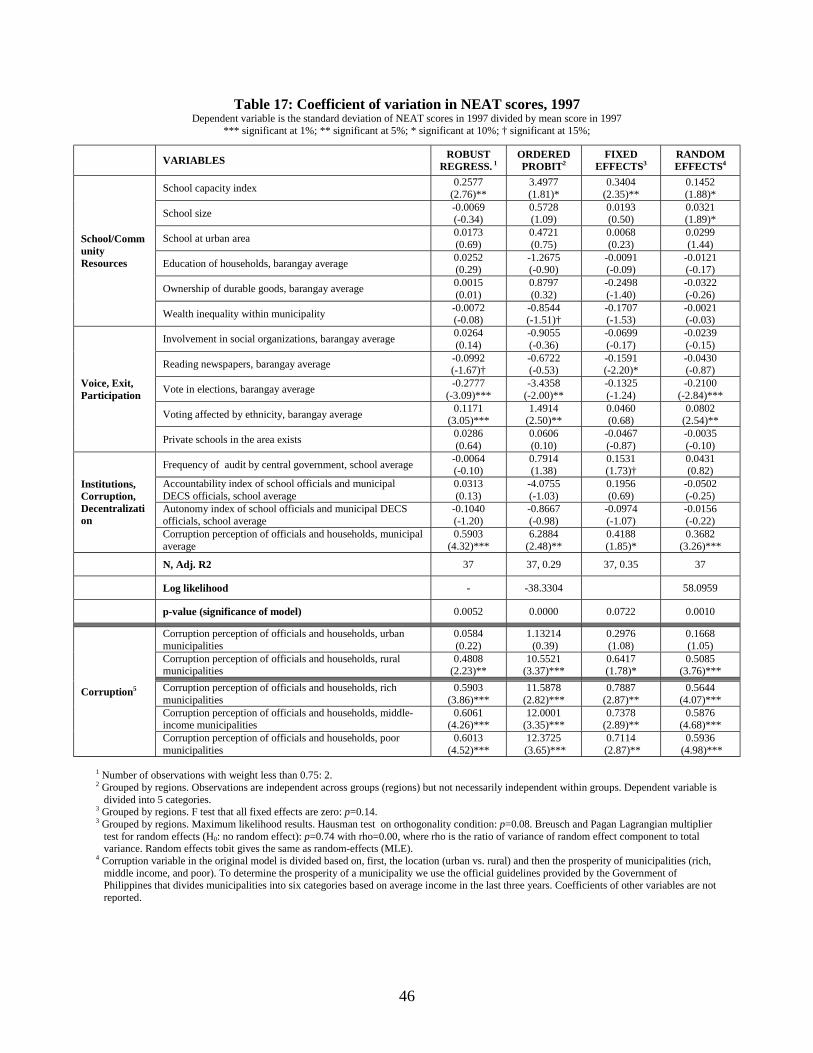
46

Table 17: Coefficient of variation in NEAT scores, 1997Dependent variable is the standard deviation of NEAT scores in 1997 divided by mean score in 1997

*** significant at 1%; ** significant at 5%; * significant at 10%; † significant at 15%;


ORDEREDPROBIT2

FIXEDEFFECTS3

RANDOMEFFECTS4

School capacity index 0.2577(2.76)**

3.4977(1.81)*

0.3404(2.35)**

0.1452(1.88)*

School size -0.0069(-0.34)

0.5728(1.09)

0.0193(0.50)

0.0321(1.89)*

School at urban area 0.0173(0.69)

0.4721(0.75)

0.0068(0.23)

0.0299(1.44)

Education of households, barangay average 0.0252(0.29)

-1.2675(-0.90)

-0.0091(-0.09)

-0.0121(-0.17)

Ownership of durable goods, barangay average 0.0015(0.01)

0.8797(0.32)

-0.2498(-1.40)

-0.0322(-0.26)



-0.8544(-1.51)†

-0.1707(-1.53)

-0.0021(-0.03)

Involvement in social organizations, barangay average 0.0264(0.14)

-0.9055(-0.36)

-0.0699(-0.17)

-0.0239(-0.15)

Reading newspapers, barangay average -0.0992(-1.67)†

-0.6722(-0.53)

-0.1591(-2.20)*

-0.0430(-0.87)

Vote in elections, barangay average -0.2777(-3.09)***

-3.4358(-2.00)**

-0.1325(-1.24)

-0.2100(-2.84)***

Voting affected by ethnicity, barangay average 0.1171(3.05)***

1.4914(2.50)**

0.0460(0.68)

0.0802(2.54)**



0.0606(0.10)

-0.0467(-0.87)

-0.0035(-0.10)

Frequency of audit by central government, school average -0.0064(-0.10)

0.7914(1.38)

0.1531(1.73)†

0.0431(0.82)

Accountability index of school officials and municipalDECS officials, school average

0.0313(0.13)

-4.0755(-1.03)

0.1956(0.69)

-0.0502(-0.25)

Autonomy index of school officials and municipal DECSofficials, school average

-0.1040(-1.20)

-0.8667(-0.98)

-0.0974(-1.07)

-0.0156(-0.22)


Corruption perception of officials and households, municipalaverage

0.5903(4.32)***

6.2884(2.48)**

0.4188(1.85)*

0.3682(3.26)***

N, Adj. R2 37 37, 0.29 37, 0.35 37

Log likelihood - -38.3304 58.0959


Corruption perception of officials and households, urbanmunicipalities

0.0584(0.22)

1.13214 (0.39)

0.2976(1.08)

0.1668(1.05)

Corruption perception of officials and households, ruralmunicipalities

0.4808(2.23)**

10.5521(3.37)***

0.6417(1.78)*

0.5085(3.76)***

Corruption perception of officials and households, richmunicipalities

0.5903(3.86)***

11.5878(2.82)***

0.7887(2.87)**

0.5644(4.07)***

Corruption perception of officials and households, middle-income municipalities

0.6061(4.26)***

12.0001(3.35)***

0.7378(2.89)**

0.5876(4.68)***

Corruption5

Corruption perception of officials and households, poormunicipalities

0.6013(4.52)***

12.3725 (3.65)***

0.7114 (2.87)**

0.5936 (4.98)***



test for random effects (H0: no random effect): p=0.74 with rho=0.00, where rho is the ratio of variance of random effect component to totalvariance. Random effects tobit gives the same as random-effects (MLE).


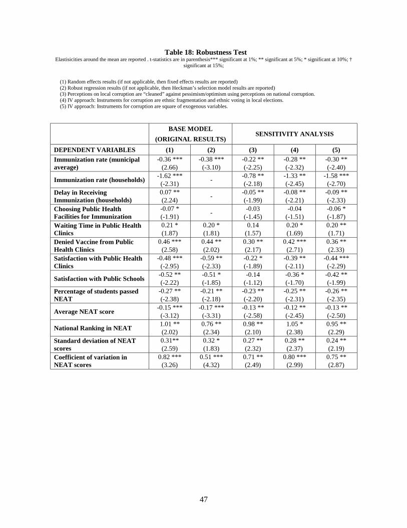
47

Table 18: Robustness TestElastisicities around the mean are reported . t-statistics are in parenthesis*** significant at 1%; ** significant at 5%; * significant at 10%; †

significant at 15%;

(1) Random effects results (if not applicable, then fixed effects results are reported)(2) Robust regression results (if not applicable, then Heckman’s selection model results are reported)(3) Perceptions on local corruption are “cleaned” against pessimism/optimism using perceptions on national corruption.(4) IV approach: Instruments for corruption are ethnic fragmentation and ethnic voting in local elections.(5) IV approach: Instruments for corruption are square of exogenous variables.

BASE MODEL(ORIGINAL RESULTS)

SENSITIVITY ANALYSIS

DEPENDENT VARIABLES (1) (2) (3) (4) (5)Immunization rate (municipalaverage)

-0.36 ***(2.66)

-0.38 ***(-3.10)

-0.22 **(-2.25)

-0.28 **(-2.32)

-0.30 **(-2.40)

Immunization rate (households) -1.62 ***(-2.31) - -0.78 **

(-2.18)-1.33 **(-2.45)

-1.58 ***(-2.70)

Delay in ReceivingImmunization (households)

0.07 **(2.24) - -0.05 **

(-1.99)-0.08 **(-2.21)

-0.09 **(-2.33)

Choosing Public HealthFacilities for Immunization

-0.07 *(-1.91) - -0.03

(-1.45)-0.04

(-1.51)-0.06 *(-1.87)

Waiting Time in Public HealthClinics

0.21 *(1.87)

0.20 *(1.81)

0.14(1.57)

0.20 *(1.69)

0.20 **(1.71)

Denied Vaccine from PublicHealth Clinics

0.46 ***(2.58)

0.44 **(2.02)

0.30 **(2.17)

0.42 ***(2.71)

0.36 **(2.33)

Satisfaction with Public HealthClinics

-0.48 ***(-2.95)

-0.59 **(-2.33)

-0.22 *(-1.89)

-0.39 **(-2.11)

-0.44 ***(-2.29)

Satisfaction with Public Schools -0.52 **(-2.22)

-0.51 *(-1.85)

-0.14(-1.12)

-0.36 *(-1.70)

-0.42 **(-1.99)

Percentage of students passedNEAT

-0.27 **(-2.38)

-0.21 **(-2.18)

-0.23 **(-2.20)

-0.25 **(-2.31)

-0.26 **(-2.35)

Average NEAT score -0.15 ***(-3.12)

-0.17 ***(-3.31)

-0.13 **(-2.58)

-0.12 **(-2.45)

-0.13 **(-2.50)

National Ranking in NEAT 1.01 **(2.02)

0.76 **(2.34)

0.98 **(2.10)

1.05 *(2.38)

0.95 **(2.29)

Standard deviation of NEATscores

0.31**(2.59)

0.32 *(1.83)

0.27 **(2.32)

0.28 **(2.37)

0.24 **(2.19)

Coefficient of variation inNEAT scores

0.82 ***(3.26)

0.51 ***(4.32)

0.71 **(2.49)

0.80 ***(2.99)

0.75 **(2.87)

Documents

Does Corruption Affect Health and Education - United …unpan1.un.org/intradoc/groups/public/documents/... · Does Corruption Affect Health and Education Outcomes in the Philippines?