Working Paper Researchby Yassine Bakkar, Olivier De Jonghe and Amine Tarazi

March 2019 No 369

Does banks’ systemic importance affect their capital structure and balance

sheet adjustment processes ?

NBB WORKING PAPER No. 369 – MARCH 2019

Editor

Pierre Wunsch, Governor of the National Bank of Belgium

Statement of purpose:

The purpose of these working papers is to promote the circulation of research results (Research Series) and analyticalstudies (Documents Series) made within the National Bank of Belgium or presented by external economists in seminars,conferences and conventions organised by the Bank. The aim is therefore to provide a platform for discussion. The opinionsexpressed are strictly those of the authors and do not necessarily reflect the views of the National Bank of Belgium.

The Working Papers are available on the website of the Bank: http://www.nbb.be

© National Bank of Belgium, Brussels

All rights reserved.Reproduction for educational and non-commercial purposes is permitted provided that the source is acknowledged.

ISSN: 1375-680X (print)ISSN: 1784-2476 (online)

NBB WORKING PAPER No. 369 – MARCH 2019

Abstract

Frictions prevent banks to immediately adjust their capital ratio towards their desired and/orimposed level. This paper analyzes (i) whether or not these frictions are larger for regulatory capitalratios vis-à-vis a plain leverage ratio; (ii) which adjustment channels banks use to adjust their capitalratio; and (iii) how the speed of adjustment and adjustment channels differ between large, systemicand complex banks versus small banks. Our results, obtained using a sample of listed banks acrossOECD countries for the 2001-2012 period, bear critical policy implications for the implementation ofnew (systemic risk-based) capital requirements and their impact on banks’ balance sheets,specifically lending, and hence the real economy.

JEL classification: G20, G21; G28.

Keywords: capital structure, speed of adjustment, systemic risk, systemic size, bank regulation,

lending, balance sheet composition.

Authors:Yassine Bakkar, Université de Limoges, LAPE – e-mail: yassine.bakkar@unilim.fr

Olivier De Jonghe (corresponding author), Economics and Research Department, NBB andEuropean Banking Center, Tilburg University – e-mail: olivier.dejonghe@nbb.be

Amine Tarazi, Université de Limoges, LAPE and Institut Universitaire de France (IUF)– e-mail: amine.tarazi@unilim.fr

The authors would like to thank two referees as well as Sebastian de-Ramon, Bob De Young,Iftekhar Hasan, Kose John and participants at the IFABS Asia 2017 Ningbo conference, the 2018VSBF Hue conference and the 2018 SEABC Palembang conference, for helpful comments andsuggestions. We also acknowledge financial support from the Europlace Institute of Finance, LouisBachelier.

The views expressed in this paper are those of the authors and do not necessarily reflect the viewsof the National Bank of Belgium or any other institution to which the authors are affiliated.

NBB WORKING PAPER No. 369 – MARCH 2019

NBB WORKING PAPER – No. 369 - MARCH 2019

TABLE OF CONTENTS

1. Introduction ............................................................................................................................... 1

2. Data: sample and variables ....................................................................................................... 5

2.1. Sample selection .................................................................................................................. 5

2.2. Bank capital, size and systemic risk...................................................................................... 5

3. Leverage versus regulatory capital requirements: dynamic adjustment mechanisms ................. 8

3.1. Inferring adjustment speeds and implied targets: a partial adjustment model ........................ 83.2. Balance sheet adjustment mechanisms .............................................................................. 12

4. Bank capital adjustments: are SIFIs different? ......................................................................... 17

4.1. Do SIFIs adjust their capital ratios quicker? ........................................................................ 18

4.2. Does regulatory pressure affect (SIFIs) adjustment speeds? .............................................. 22

4.3. Do SIFIs use different adjustment mechanisms? ................................................................ 23

5. Robustness checks and further issues .................................................................................... 27

6. Conclusion .............................................................................................................................. 30

References .................................................................................................................................. 32Tables ........................................................................................................................................ 37

Appendix ..................................................................................................................................... 50

National Bank of Belgium - Working Papers series ....................................................................... 53

NBB WORKING PAPER No. 369 – MARCH 2019

1

1. Introduction

In the aftermath of the 2007-2008 global financial crisis, regulators have introduced

stringent changes to the regulation of banks, especially by redesigning existing frameworks for

regulatory capital requirements and by tightening the supervision of the so called systemically

important financial institutions (SIFIs)1. There is a rapidly growing literature analyzing various

specific elements of the Basel III capital requirements2 (Cecchetti (2015), Dermine (2015),

Repullo and Suarez (2013)) as well as their potential consequences for bank performance

(Giordana and Schumacher (2012), Berger and Bouwman (2013), Admati et al. (2010)), bank risk-

taking (Kiema and Jokivuolle (2014), Hamadi (2016)), economic and financial stability (Angelini

et al. (2014), Rubio and Carrasco-Gallego (2016), Farhi and Tirole (2012), Acharya and Thakor

(2016), Hanson et al. (2011), Brunnermeier and Pederson (2009)), and credit supply (e.g.

Cosimano and Hakura (2011), Jimenez et al. (2017), De Jonghe et al. (2016), Kok and Schepens

(2013), Francis and Osborne (2012), Ivashina and Scharfstein (2010)).

While this first stream of papers is interested in the equilibrium implications of capital

requirements, there is another stream that investigates the dynamics of bank capital towards a new

equilibrium. This other stream of research has analyzed how quickly banks can adjust their capital

ratios and which mechanisms they can resort to (see e.g., Berger et al. (2008), Memmel and

Raupach (2010), Öztekin and Flannery (2012), Lepetit et al. (2015), De Jonghe and Öztekin

(2015), Cohen and Scatigna (2016)).

We link these two strands of literature and aim to fill two specific gaps in the existing

literature. First of all, we address the following questions: Are there differences in adjustment

mechanisms and adjustment speed for leverage vis-à-vis regulatory capital? Might they conflict?

Although banks cannot set their desired leverage ratio ignoring the restrictions imposed by

regulatory ratios, how and how quickly they adjust to leverage and regulatory ratios can differ

1

According to the definition of the Financial Stability Board, systemically important financial institutions (SIFIs) are

financial institutions whose distress or disorderly failure, because of their size, complexity and systemic

interconnectedness, would cause significant disruption to the wider financial system and economic activity. 2 Regarding capital requirements, the most important innovations in Basel III are the introduction of a leverage

requirement (next to risk-weighted capital requirements), a capital surcharge for systemically important banks and the

introduction of a countercyclical capital buffer. The imposed changes aspire to achieve financial stability by

increasing the resilience of banks to shocks and by forcing them to internalize systemic externalities.

2

because of conflicting pressures from shareholders and regulators. Second, while this first step

results in unconditional, homogenous results describing average bank behavior, we subsequently

differentiate between SIFI banks and non-SIFI banks, given the new regulatory and supervisory

focus on the two groups. We analyze, both for leverage and risk-weighted capital ratios, whether

systemically important financial institutions behave differently in terms of adjustment mechanisms

and adjustment speed.

In the first part of the analysis, we focus on differences in adjustments of a leverage ratio,

i.e. the equity-to-total (unweighted) asset ratio, and two regulatory capital ratios (Tier 1 capital

over risk-weighted assets and total capital over risk-weighted assets) for OECD banks. We follow

the literature and estimate a partial adjustment model of bank capital towards a bank-specific and

time-varying optimal capital ratio (see e.g. Berger et al., (2008), Memmel and Raupach (2010),

Öztekin and Flannery (2012), Lepetit et al. (2015), De Jonghe and Öztekin (2015)). The partial

adjustment model assumes that banks do have a target3 (or optimal) capital ratio, but that there

might be frictions (such as adjustment costs) that prevent them from instantaneously adjusting

towards the target. Hence, at each point in time, the actual capital ratio is a weighted average of

the lagged capital ratio and the target capital ratio, where the weight is an indication of the

magnitude of the frictions. It is ex-ante unclear whether the speed of adjustment should be higher

for the regulatory capital ratios versus the leverage ratio. On the one hand, one could expect a

faster adjustment for the Tier 1 and Total Capital ratio than for the leverage ratio given the

regulatory focus on these measures. On the other hand, the opposite could also be found because

the set of adjustment mechanisms is smaller for the regulatory capital ratios vis-à-vis the leverage

ratio, as not all types of equity count and because assets vary in risk weight. For example,

government bonds (of OECD countries) are securities that are easily adjustable, but have a zero risk-

weight. They could help to adjust the leverage ratio, but not the regulatory capital ratios.

Our findings show that banks are more flexible and faster in adjusting the common equity

capital ratio than regulatory capital ratios. More specifically, in our sample of listed OECD banks

3 It is important to emphasize that, for both questions, we analyze the dynamics in banks’ capital adjustment

(mechanisms and speed) towards a bank-specific and time-varying optimal capital ratio. Such bank-specific and time-

varying optimal capital ratios are determined by the regulatory minimum as well as banks’ desire to hold a buffer over

the minimum capital requirements. Both the requirement and the buffer are time-varying and bank-specific. Moreover,

both cannot be disentangled as information on the former is not publicly available since regulators can use Pillar 2

requirements to impose bank-specific and time-varying capital requirements. However, these requirements are

typically communicated privately to the bank and they are confidential.

3

over the 2001-2012 period, the speed of adjustment for the non-weighted equity-to-asset capital

ratio structure is 0.44, which is larger than the one for the Tier 1 capital ratio, 0.29, and the total

capital ratio, 0.33. In economic terms, these speeds of adjustment correspond with half-lives of

1.18, 2.07 and 1.74 years, respectively. The half-life is computed as log(0.5)/log(1- speed of

adjustment) and is equal to the time required for banks to halve the gap between their actual

capital ratio and their target.

To understand better why the speeds of adjustment differ, we subsequently investigate how

banks manage adjustments towards their targets. The estimation procedure allows us to back out

the estimated target capital ratio and hence also the gap between the target and the actual capital

ratio. We investigate growth rates in various assets classes, liability categories and types of equity,

according to the sign of the gap for both the leverage and regulatory capital ratios. Facing an

opportunity cost, overcapitalized (underleveraged) banks have no incentives to remain above their

targeted capital ratio, i.e. hold a capital surplus over their target. Therefore, bank managers make

proactive efforts to converge to their target by reducing their capital levels. For all capital

specifications, we find that banks lever up by expanding assets, through an unrestrictive lending

policy and risk-taking preferences, increasing liabilities both with long-term and short-term

borrowings (except for the leverage ratio) and lessening equity growth, both internally (smaller

amount of retained earnings) and externally (equity repurchasing and/or less equity issues). In

contrast, when banks have a capital shortfall with comparison to their target, we find that

undercapitalized banks de-lever by an aggressive growth reduction in all its subcomponents; i.e.

loans and risk-weighted assets, but at the same time also raise capital externally.

In the second part of the analysis, we investigate whether or not systemically important

financial institutions behave differently in terms of capital structure adjustments. Although SIFIs

and large banking groups are subject to prudential regulations and considerable research has

pointed out their characteristics and performance (see e.g. Bertay et al. (2013), Barth and Schnabel

(2013), Laeven et al. (2015)), how they manage their capital structure and rebalance to converge to

their optimal capital levels remains an open question with important policy implications. Indeed,

SIFIs could behave very differently. On the one hand, because they enjoy favorable treatment from

financial markets (higher debt ratings, lower interest rates) due to their favored access to

4

government safety nets and subsidies, SIFIs might adjust their capital structure more quickly and

more frequently. On the other hand, SIFIs might not weigh the need to adjust quickly if they

expect public support and bailout or because their complexity and opacity make it costlier for them

to raise external capital.

Combining the insights from Bertay et al. (2013) and Barth and Schnabel (2013), we focus

on four distinguishing aspects of SIFIs, which are their absolute size (natural log of total assets),

their relative size (total assets over GDP), their systemic risk contributions (delta Conditional

Value-at-Risk (∆CoVaR)) and systemic risk exposures (Marginal Expected Shortfall (MES)).

SIFIs are more likely to care about their sensitivity to a sudden market shortfall than to how much

their operations might jeopardize the financial system in times of crisis. Nevertheless, regulatory

scrutiny could also be effective in pushing SIFIs to internalize the threat that they pose on the

system. We also construct a systemic risk index based on the quintiles of such indicators. We find

that systemically important banks adjust slower than other banks to their target leverage ratios but

quicker to their regulatory target ratios. When we dig into the four aspects that define SIFIs, we

find that these opposite findings on the leverage ratio and regulatory ratio are explained by the

differential impact that size and systemic risk have. Larger banks adjust slower and this effect

dominates for the leverage ratio, whereas systemically riskier banks adjust faster and more so their

regulatory capital ratios.

Moreover, our results suggest that SIFIs might be more reluctant to change their capital base by

either issuing or repurchasing equity and prefer sharper downsizing or faster expansion. Any

unexpected need for banks to raise capital ratios might therefore be more harmful for firms and

households who are clients of such large institutions. To the extent that SIFIs account for a large

portion of a banking industry (through a larger market share) the negative impact on the economy

as a whole could also be more important.

The rest of the paper proceeds as follows. Section 2 presents information on the sample

construction and variables of interest, in particular the various concepts of capital and the

measures of (systemic) size and systemic risk. In Section 3, we examine and contrast the

adjustment speed and adjustment mechanisms for various concepts of bank capital. Analyzing how

5

and how quick SIFIs adjust their balance sheet in response to deviations between the actual capital

ratio and the optimal capital ratio is performed in Section 4. Section 5 concludes.

2. Data: sample and variables

2.1. Sample selection

We conduct the analysis on a sample of listed banks headquartered in any of the OECD

countries and analyze the 2001-2012 period4. For these banks, we obtain accounting and market

data from various sources. We retrieve bank stock price information and other market data from

Bloomberg. We obtain bank-level accounting data from Thomsen-Reuters Advanced Analytics

and Bloomberg. We collect macroeconomic data from the OECD Metadata stats. Starting from the

matched accounting and market data, we further drop banks with illiquid stocks, that is banks with

infrequently traded stocks and low variability in stock prices (we disregard a stock if daily returns

are zero over five rolling consecutive days or if more than 70% of the daily returns over the period

are non-zero returns). Information on the sample composition by country and by year can be found

in panel A and B of Table 1.

[Insert Table 1 about here]

We end up with an unbalanced panel dataset of 554 banks, from the 26 major advanced

OECD countries. It consists of 407 U.S. banks and 147 non-U.S. banks, among which 112 are

European (from 22 countries) and 22 are Japanfese. Although we only consider publicly-traded

OECD banks, our sample conveniently represents the U.S., euro area and Japanese banking

sectors. The listed banks included in our sample account for approximately 73%, 52% and 31% of

the total assets of all U.S., euro zone and Japanese banks recorded in BSI/Bloomberg statistics,

respectively.

2.2. Bank capital, size and systemic risk

4 We end the sample period in 2012 in order to avoid interference with the implementation of the Basel III regulations

(starting from 2013) that among other things introduced a leverage ratio as well as capital surcharges for systemically

important banks. Doing so, we can study how banks treat regulatory capital ratios differently from plain leverage

ratios in the absence of regulation on the latter. Moreover, we are able to study differential behavior by SIFIs and

other banks in a period where the proposed methodologies for identifying G-SIFIs were not yet published for public

consultation. These were published in January 2014.

6

We focus on two types of capital measures. We focus on two regulatory capital ratios by

using the Tier1 regulatory capital ratio, defined as Tier 1 equity over total risk-weighted assets

(Tier1RWA hereafter) and the Total Capital ratio, defined as the sum of Tier 1 and Tier 2 equity to

total risk-weighted assets. We also consider the average non-weighted common equity ratio

(leverage ratio), defined as common equity over total non-weighted assets. The latter is based on

cruder risk-exposure, which may be more relevant for stock market participants or debt holders

whom may view risk weights as highly opaque and uninformative (Blum, 2008).

In our analysis, we devote special attention to Systemically Important Financial Institutions

(SIFIs, for a definition see footntote 4). A first approach to capture whether banks are systemically

important is assessing their size. Bertay et al. (2013) suggest the use of two proxies of systemic

size, namely a bank’s absolute size, defined as the logarithm of a bank’s total assets, as well as a

bank’s relative size, defined as a bank’s total assets over gross domestic product (GDP). Barth and

Schnabel (2013) argue and document that bank size (be it absolute or relative) is not a sufficient

measure of systemic risk because it neglects aspects such as interconnectedness, correlation, and

the economic context. They suggest the use of market-based measures of systemic importance,

such as the delta Conditional Value-at-Risk (∆CoVaR, by Adrian and Brunnermeier (2016)),

which captures the contribution to system wide risk of an individual bank, or a measure of an

individual bank’s systemic risk vulnerability/exposure to system wide distress such as the

Marginal Expected Shortfall (MES, see Acharya et al. 2016 and Brownlees and Engle, 2012). The

difference between the two concepts is the directionality. The former assesses the extent to which

distress at a bank contributes to system-wide stress, whereas the latter identifies the extent to

which a bank’s stock will lose value when there is a systemic event. The MES and ∆CovaR will

typically be positive (we use the opposite of returns such that losses are expressed with a positive

sign) and higher values correspond to larger systemic risk exposures and contributions. More

information on the construction of these measures is in appendix A1 and the papers referenced

therein.

We also construct a composite SIFI-index that covers in an equally-weighted way these

four dimensions of systemic importance: a proxy of absolute size, systemic size, systemic

exposure and contagion risk. More specifically, for each of the four metrics, we divide the sample

in quintiles and give a score of one to banks in the lowest quintile, two in the second quintile and

so on, with five for the highest. Subsequently, we take the sum of the scores associated to each of

7

these quintiles of the four size or risk metrics to obtain an index that ranges from four to twenty,

with the highest value representing the highest level of systemic importance that an individual

bank can exhibit. This equally-weighted index of four characteristics provides a summary statistic

of systemic importance because it combines several measures of systemic risk and size in one

metric.

Panel A of Table 2 reports definitions, sources and summary statistics on the bank-level

capital ratios and the control variables we use in our estimations. All variables are winsorized at

the top and bottom 1 percent level to eliminate the adverse effects of outliers and misreported data.

The average leverage, Tier1RWA and Total Capital ratios are 9.3%, 11.7% and 14.1%,

respectively. Furthermore, the fifth percentile of the Tier1RWA and Total Capital ratio suggests

that regulatory capital ratios are well above the Pillar 1 minimum requirement for the majority of

banks throughout the sample period.

In panel A, we also provide descriptive statistics for the bank-level variables we use to

examine the determinants of banks’ target capital ratios. Overall, across the sample period and

countries, we observe that the average bank has low credit risk (average loan loss provisions to

total loans of 0.7%), is strongly reliant on retail market funding (89.7%), is reasonably liquid as

indicated by the ratio of net loans to total deposits (108.9%), has a low amount of fixed assets

(1.6%), is moderately diversified in terms of assets (average loans to assets is 69%) and revenue

(average non-interest income share is 19.6%). In terms of insolvency risk (bank default risk) and

riskiness of assets, the average bank is relatively sound (average market-based Z-score is 3.43) but

allocates a large fraction of its assets to high risk-weight assets (average risk-weighted asset ratio

is 73.8%).

[Insert Table 2 about here]

Panel B of Table 2 presents the summary statistics of systemic risk and size measures at the

individual bank level for the full sample period. The mean of the natural logarithm of total book

assets is 8.15 and the median is 7.42 (which correspond to about $3 billion and $2 billion

respectively). Although we only consider publicly traded OECD banks, our sample still exhibits

considerable size heterogeneity across banks. This is clear from the standard deviation (2.311) and

8

the range between the 5th

percentile and the 95th

percentile [5.585 to 13.010]. The relative bank

size measure confirms the heterogeneity across banks and the presence of large banks relative to a

country’s economic importance. For example, relative size varies between 0.00% (fifth percentile)

and 51.8% (95th

percentile) out of the domestic GDP, with a standard deviation of 19.7%. The

summary statistics also reveal that banks vary in terms of systemic importance. The average values

of MES and ∆CoVaR are 1.69% and 1.56% but the systemic risk measures are disperse with

standard deviations of 1.91% and 1.74%, respectively.

Table 3 presents pairwise correlations among all variables at the bank level.

[Insert Table 3 about here]

3. Leverage versus regulatory capital requirements: dynamic adjustment mechanisms

3.1. Inferring adjustment speeds and implied targets: a partial adjustment model

In a frictionless world, banks would always maintain their target capital ratio. However, if

adjustment costs are significant, the bank’s decision to adjust its capital structure depends on the

trade-off between the adjustment costs and the costs of operating with suboptimal leverage

(Flannery and Rangan (2006), Flannery and Hankins (2013)). To allow for sluggish adjustment, it

has become common practice in the empirical (corporate and bank) capital structure literature to

model leverage using a partial adjustment framework (see e.g., Flannery and Rangan (2006),

Lemmon et al. (2008), Gropp and Heider (2010), De Jonghe and Öztekin (2015) and Lepetit et al.

(2015)). In a partial adjustment model, a bank’s current capital ratio, Kij,t, is a weighted average

(with weight λ ϵ [0,1]) of its target capital ratio, Kij,t∗ , and the previous period’s capital ratio,

Kij,t−1, as well as a random shock, εij,t:

(1) Kij,t = λKij,t∗ + (1 − λ)Kij,t−1 + εij,t

where ij,t indicates bank i from country j in year t. Each year, the typical bank closes a

proportion λ of the gap between its actual and target capital levels. The smaller the lambda, the

more rigid bank capital is, and the longer it takes for a bank to return to its target after a shock to

9

bank capital. Thus, we can interpret λ as the speed of adjustment and its complement (1 − λ) as

the portion of capital that is inertial.

Banks’ target capital ratio, Kij,t∗ , is unobserved and is not necessarily constant over time. It

consists of two building blocks: a linear combination of observed (lagged, hence time t−1) bank

and country characteristics, Xij,t−1, as well as bank and time fixed effects.

(1) Kij,t∗ = βXij,t−1 + vt + ui

For the set of bank characteristics we build on Gropp and Heider (2010) who show that

standard cross-sectional determinants of non-financial firms’ leverage carry over to banks. These

determinants and their relation to (bank) capital are based on departures from the Modigliani-

Miller irrelevance proposition because of market imperfections and highlighted by various

corporate finance theories (see Harris and Raviv, 1991 and Frank and Goyal, 2008, for surveys).

We therefore include proxies for bank size (diversification benefits and cost of external finance),

bank profitability (pecking order theory), overall risk (trade-off theory), fixed assets (collateral)

and non-interest income (growth opportunities). In addition, we follow Berger et al. (2012) and

include various proxies for exposures to counterparty risk (retail funding and loan to assets). A

greater reliance on insured retail deposits should reduce pressure from counterparties to hold more

capital. Business borrowers prefer well-capitalized lenders because borrower–lender relationships

are costly to replace if the lender fails. There is ex-ante no theoretical or empirical guidance to

decide on altering the set of factors for the leverage ratio vis-à-vis the regulatory capital ratios.

Berger et al. (2008) and Gropp and Heider (2010), for example, also examine both leverage and

regulatory capital ratios and do not differentiate between the set of explanatory variables for both

types of capital ratios. Therefore, we also use the same set of factors for each capital ratio.5

5 The specific ratios that we include are: bank absolute size (natural logarithm of total assets), bank profitability

(return on assets), bank credit risk (loan loss provisions to net loans), retail funding (customer deposits to total

funding), liquidity ratio (net loans to total assets). We also include the ratio of fixed assets to total assets, a

diversification proxy (non-interest income to total income), a bank efficiency proxy (non-interest expense to total

income), a ratio of risk-weighted assets over total assets and a market-based Z-score. Subsets of these are also used in

other papers (Lepetit et al. (2015), Francis and Osborne (2012), Lemmon et al. (2008), Flannery and and Rangan

(2006)).

10

We also account for two sources of unobserved heterogeneity: vt is a vector of year fixed

effects. ui is a vector of bank fixed effects (which subsume country fixed effects) and capture

unobserved heterogeneity such as quality of management, governance, risk preference and the mix

of markets in which the bank operates. The inclusion of bank (or firm) fixed effects in capital

structure regressions is econometrically and economically important. Flannery and Rangan (2006),

Lemmon et al. (2008), Huang and Ritter (2009), and Gropp and Heider (2010) advocate the

importance of including bank (or firm) dummies for an unbiased estimation of targets. They have

also shown that capital ratios tend to fluctuate around a bank specific time-invariant parameter,

which can be viewed as a long-term target. In fact, De Jonghe and Öztekin (2015) report for a

sample of worldwide banks that the fraction of the total variation in banks’ capital ratios due to

time-invariant bank characteristics (bank fixed effects) is 85%. This is similar to what is found for

US non-financial firms by Lemmon et al. (2008) and for US and European banks by Gropp and

Heider (2010). Hence, an extremely important component of a bank’s leverage and regulatory

target capital ratios is thus a bank fixed effect.

Substituting the equation of target leverage, equation (2), in equation (1) yields the

following specification:

(2) Kij,t = λ(βXij,t−1 + vt + ui) + (1 − λ)Kij,t−1 + εij,t.

In the presence of a lagged dependent variable and a short panel, using ordinary least

squares (OLS) or a standard fixed effects model would yield biased estimates of the adjustment

speed. Therefore, following Flannery and Hankins (2013), we estimate equation (3) using Blundell

and Bond's (1998) generalized method of moments (GMM) estimator.

We estimate the partial adjustment model of equation (3) separately for each of the three

alternative capital ratios: Leverage, Tier1RWA and Total capital. The results are reported in Table

4.

[Insert Table 4 about here]

11

We focus the description of the results on the variable of interest, which is the coefficient

on the lagged dependent variable.6,7 The estimated adjustment speeds (𝜆, Eq. (3)) are significant

and quite different for the three capital ratio models. The speed of adjustment for the non-weighted

equity-to-asset capital ratio structure is 0.444 (=1–0.556, where 0.556 is the coefficient of the

lagged equity-to-asset reported in the first column). This speeds of adjustment is similar to those of

European banks (0.34, Lepetit, et al., 2015), a sample of banks in the U.S. and 15 European

countries (0.47, Gropp and Heider, 2010), and large U.S. banks (0.40, Berger et al., 2008).

The adjustment speed for the regulatory capital ratios is lower, namely 0.285 (1-0.715, column 2)

for the Tier 1 RWA ratio and 0.328 (1-0.672, column 3) for the total capital ratio. This implies that

adjustment is partial for each of the capital ratios, but faster when banks are closing the equity-to-

asset ratio deviation during the next period t, than when they are closing the two regulatory capital

deviations (columns 2 and 3). Another informative metric, which provides economic meaning to

the estimated parameters, is the half-life. The half-life provides an indication of the time required

for banks to halve the gap between their actual capital ratio and their target. The estimated

adjustment speeds for the leverage, Tier1 RWA and total capital ratios deviations correspond with

half-lives of 1.18, 2.07 and 1.74 years, respectively. The results highlight that banks are slightly

more concerned about readjusting quickly towards optimal leverage ratios compared to the speed

to adjust towards optimal regulatory capital. This finding can be rationalized by at least two

arguments. On the one hand, it could indicate that deviations from optimal leverage ratios are

more costly for bank shareholders (as the target capital should be chosen such to maximize bank

value) than deviations from regulatory capital. On the other hand, it could also be created by

differences in adjustment costs and the range of adjustment mechanism that can be used. All else

equal, banks have more (and less costly) options in asset adjustments that affect non-risk weighted

6 For each model, we also report the coefficient estimates and the significance levels of bank-specific drivers of the

target capital ratios. Smaller banks, banks with more credit risk and banks with more asset diversification (less loans)

hold higher capital ratios. Besides, less liquid banks and banks with more retail funding have a higher equity-to-target

ratio, but not higher regulatory capital ratios. Nor the ratio of risk-weighted assets to total assets neither the Z-score

enter significantly, likely because of the high correlation with other bank characteristics. However, we do include

them as they are important theoretical drivers of target leverage (trade-off theory) and because they are important for

obtaining accurate speed of adjustment estimates. 7 At the bottom of panel A of Table 4, we report test statistics documenting the validity of the instruments. In

particular, two crucial tests are required. Using the Hansen J test (test of exogeneity of the instruments), we cannot

reject the null of joint validity of all GMM instruments (lagged values); we hence confirm the validity of the

instruments. We also use the Arellano and Bond AR(2) test, and confirm the absence of second order serial

autocorrelation in the residuals.

12

assets than risk-weighted assets. For example, government bonds (of OECD countries) are

securities that are easily adjustable, but have a zero risk-weight. They could help to adjust the

leverage ratio, but not the regulatory capital ratios.

3.2. Balance sheet adjustment mechanisms

In this section, we investigate how banks adjust their capital structure to close their

deviation (gap) from the target. To do that, we use the following procedure. Based on the

estimated vector of coefficients �� from equation (3) we can compute fitted time-varying target

capital ratios for each individual bank, 𝐾 𝑖,𝑗,𝑡∗ . Subsequently, we compute the time-varying capital

deviation for bank i at time t-1, hereinafter called “the gap”, and defined as 𝐺𝐴𝑃𝑖𝑗,𝑗,𝑡−1= ��𝑖𝑗,𝑡∗ −

𝐾𝑖𝑗,𝑡−1. Therefore, according to equation (3), the bank fixed effects are part of these estimated

targets and gaps. If banks make adjustments when there is a gap, then these adjustments should be

reflected in their observed balance sheet transactions. We follow the approach of De Jonghe and

Öztekin (2015) and evaluate the percentage growth rates in various balance sheet components for

three quintiles of the gap (first, middle and fifth). To do this, we first allocate banks to quintiles

based on their gap at the end of year. Subsequently, we compute the yearly change in the relevant

variable in the following year. We then average these growth rates across all bank-year

observations in that quintile.

In a first step, we analyze the balance sheet adjustments for each capital ratio separately

(subsection 3.2.1). These results are reported in Table 5. In a second step (subsection 3.2.2), we

examine balance sheet adjustments in situations where the gap of the leverage ratio and Tier 1

RWA ratio have similar or opposite signs, yielding four cases; (i) both signal overcapitalization,

(ii) both signal undercapitalization, (3) overcapitalized leverage, but undercapitalized regulatory,

and (4) undercapitalized leverage, but overcapitalized regulatory.

3.2.1. Balance sheet adjustments following a leverage or regulatory capital gap

13

Table 5 presents the average growth rates of the main balance sheet items for banks

allocated to the first quintile (i.e. most overcapitalized/underleveraged banks), the third quintile

(i.e. banks with a negligible gap) and the fifth quintile (i.e. most undercapitalized/overleveraged

banks) based on their gap at the end of year. For each capital ratio, we report the p-values of

difference in means tests using the third quintile as benchmark. The p-values are obtained by a

bootstrap procedure using 500 replications to correct for the estimated nature of banks’ target

capital ratio (see Pagan, 1984). This bootstrap approach has become common practice in the

empirical literature using partial adjustment models for corporate capital structure (see e.g.,

Faulkender et al., 2012; Çolak et al., 2018).

[Insert Table 5 about here]

First, with respect to the leverage ratio, overcapitalized (underleveraged) banks (Q1) have a

negative and significant change in leverage ratio compared with the change rate of the third

quintile (-2.19% vs. 0.07%), implying that banks reduce their capital ratio to reach their target

capital level. In fact, facing an opportunity cost, banks have no incentives to remain above their

targeted leverage ratio. Therefore, bank managers make proactive efforts to lever up so to

converge to their target and reduce the ongoing costs of capital surplus accordingly. To achieve a

negative capital growth, our results show for a global sample of banks that they significantly

expand their asset growth (21.78% vs. 8.19%), debt growth (10.43% vs. 8.17%), while equity

growth is significantly slowed down (4.37% vs. 8.89%) always compared to the growth rates in

the third quintile (i.e. when the gap between actual and target capital is negligible). Analyzing the

mechanisms through which those banks lever up, the results indicate that underleveraged banks

progress by increasing loans (6.25%) and to a smaller (economic) extent also long-term debt

(1.87%). We note that the average loan growth and riskier assets are not economically

significantly different with respect to the growth rate of the third quintile (5.75% and 5.43%,

respectively). In the same line, banks having a capital surplus shrink their internal funding, the

growth in bank retained earnings is roughly one (1.09%), and the external funding (Tier1) growth

is substantially lowered (4.79% vis-à-vis 8.60%). Such results indicate that banks tend to lever up

by engaging more in risky activities, being financed more with long-term debt, but without

engaging any significant change in their loan policy or reduction in the capital level.

14

In contrast, for undercapitalized (overleveraged) banks (Q5), results show that the change

in leverage ratio is significantly larger (2.08% vs. 0.07%) than the third quintile, implying that

bank managers also actively rebalance their capital ratios to revert to their targeted leverage when

they are undercapitalized. To that extent, facing regulatory and market constraints, banks with a

capital shortfall are more prone to deleverage in order to close the gap and get to their optimal

target. More specifically, results for those undercapitalized banks show that the average asset

expansion is significantly negative (-7.69% vs. 8.19%) and the average debt growth is significantly

lower (4.73% vs. 8.17%), while the average equity growth is not significantly higher than the

growth rate of the benchmark. Not surprisingly, this translates into a rationalized capital

adjustment for banks to reach their leverage capital target, only by reducing assets rather than

injecting external equity which is costly because of frictions and governance problems.

On the whole, what would actually pose a problem to the real economy is if lending falls

when banks are undercapitalized but does not actually increase when they are overcapitalized. We

notice that the average growth of loans (2.87% vs. 5.75%) and riskier assets (4.41% vs. 5.43%) are

significantly lower than the benchmark. Indeed, deleveraging is achieved by downsizing (selling

assets), restricting loan policy (reducing lending vis-à-vis a lower amount of debt) and lowering

risk-weighted assets (substituting riskier assets for safer ones).

Second, with respect to regulatory capital ratio (Tier1RWA), overcapitalized banks (Q1)

have a negative growth in the Tier1 capital ratio which is significantly different from the change

rate in the third quintile of the gap (-0.97% vs. 0.18%). Hence, we inspect growth rates of

adjustment mechanisms that lead these banks to reduce their capital surplus to converge to their

optimal regulatory level. Findings show that banks allocated in this quantile lever up by a large

and significant increase of their asset growth (12.62% vs. 8.02%), debt growth (11.35% vs.

8.40%), while their equity growth is significantly lower (5.96% vs. 8.89%) compared to the

growth rates of the benchmark. Thus, overcapitalized banks proceed by significantly altering all

the subcomponents of the balance sheet with regards to the benchmark. This translates into an

expansionary growth rate (relative to Q3) in loans (7.92%), risky assets (9.40%) and long-term

debt (1.74%); and a slow-down in internal capital (1.53%) and external capital (4.19%) growth

relative to banks in the middle quintile of the regulatory gap distribution. Therefore, a Tier1 capital

15

surplus leads banks to lever up by combinations of an asset expansion strategy, risk-taking

activities, an aggressive lending policy, long and short-term debt financing policies and a slower

equity growth but without engaging any reduction in the capital level.

Concerning the regulatory undercapitalized banks (Q1), the results show that their Tier 1

regulatory capital change is significantly higher (1.23%) than the change rate of the banks in the

third quintile (0.18%). Accordingly, banks are expected to increase their regulatory capital, so to

reach their internal regulatory capital target and to comply with capital requirements. They

proceed by significantly shrinking asset growth (1.95% vs. 8.02%) and debt growth (4.78% vs.

8.40%) compared with growth rates of the benchmark, and only a moderate increase in the growth

rate of equity (p-value of 0.11). Based on these results, we then analyze the key mechanisms

through which these banks de-lever and rebalance their capital structure. Similarly, we find that

these banks react actively by significantly altering all the subcomponents of the balance sheet,

with regards to the benchmark. Results show that the loan growth (2.17%), risky asset growth

(1.83%), long-term debt (0.26%) and short-term debts (-0.68%) are significantly lower than the

growth rates of the benchmark (Q3), while the external capital growth (12.28%) is significantly

larger than the benchmark (Q3). Thus, facing a regulatory capital shortfall, deleveraging takes

place by injecting external capital (equity issues), but not by using internal capital (earnings

retention). Deleveraging is also achieved by downsizing, tightening lending policy (reducing

lending vis-à-vis a lower amount of debt), selling risky assets and reducing long and short-term

financing (selling debts). In the rightmost panel, we also show the adjustment mechanisms for the

total capital ratio. They are by and large similar to the ones of the Tier 1 risk-weighted capital ratio

(if anything, we find stronger significant differences) and are for the sake of space not discussed

here.

Finally, the results and capital management patterns of the total capital ratio are unreported but are

similar to the ones discussed above for the Tier1RWA regulatory capital ratio.

3.2.2. Balance sheet adjustments: joint stance of the leverage and regulatory gap

As the leverage ratio and regulatory capital ratios share aspects both in the numerator and

the denominator it is likely that banks do not treat them independently. We therefore now turn to

16

an analysis of balance sheet adjustments when examining the joint stance of the leverage gap and

the regulatory capital (Tier 1 capital over risk-weighted assets) gap. The results are reported in

Table 6. The four blocks of columns correspond with the situations where (i) both signal

overcapitalization, (ii) both signal undercapitalization, (iii) overcapitalized leverage ratio, but

undercapitalized regulatory ratio, and (iv) undercapitalized leverage ratio, but overcapitalized

regulatory ratio.

[Insert Table 6 about here]

Table 6 shows that when both capital ratios show overcapitalization (Group 1), banks’

equity growth is significantly lower, while asset growth and debt growth are significantly larger

than when both capital ratios show undercapitalization (Group 2). In line with previous results,

overcapitalized banks mainly lever up by expanding all assets and liabilities items, loans (7.60%),

risky asset (8.28%), long-term debt (1.97%) and short-term debt (0.86%), which are statistically

larger than the growth rates of the group of undercapitalized banks. In contrast, deleveraging for

undercapitalized banks (Group 2) is more likely achieved by external capital (10.81%) and earning

retention (3.07%), which are statistically larger than the growth rates of the group of

overcapitalized banks (column 5).

Now, we investigate the main disparities between these two groups of banks with two other

groups that are regulatory overcapitalized but undercapitalized with regards to the leverage ratio,

or vice-versa (Groups 3 and 4). Test results for equality of means test are reported in the rightmost

panel (columns 6 to 10). First, we explore differences with regards to Group 1. Underleveraged but

regulatory undercapitalized banks (Group 3) have a significantly smaller asset growth compared to

Group 1, and this is true for all their subcomponents (loans and risky assets) and liabilities growth

(only short-term debt) compared to the growth rates of the overcapitalized banks (Group 1).

However, in economic terms, we especially notice differences in the adjustments via loan growth

and risk-weighted assets. Banks in Group 3 increase leverage mainly by expanding assets with low

risk-weights. Regarding equity growth, their external capital growth is significantly larger

compared to the growth rate of banks in Group 1. However, although the non-significant lower

growth of earnings retention (1.31% vs. 1.72%) of banks in Group 3 (with regards to Group 1), the

growth of equity remains significant. Thus, to increase their regulatory capital, besides raising

17

more external capital and decreasing risky assets, banks in Group 3 restrict their lending and long-

and short-term financing policies.

However, capital management of the banks in Group 4 (overleveraged but regulatory

overcapitalized) differ from those in Groups 1 and 3. They are overleveraged, but regulatory

overcapitalized (with respect to their target). Compared to underleveraged banks, their assets grow

much less quickly and relatively speaking they rely more on earnings retention than external

capital growth. Most strikingly is that the growth in net loans and risk-weighted assets is of similar

magnitude in group 1 and 4, even though total asset growth in group 4 is much smaller compared

to growth in group 1. Hence, when they are regulatory overcapitalized, but also overlevered, they

will raise equity internally and most of the asset growth will be realized via high risk-weight

assets.

In sum, this analysis provides interesting insights in the mechanisms and the relative

dominance of leverage vis-à-vis risk-weighted capital ratios. The sign of the leverage and risk-

weighted capital ratio gap determines whether equity is adjusted via earnings retention (leverage

dominates regulatory capital) or externally raised equity (regulatory stance matters). Moreover, it

also determines whether asset side adjustments are done via loans and risky assets (regulatory gap

matters), versus safer assets with a lower risk weight (such as securities).

4. Bank capital adjustments: are SIFIs different?

The adjustment speed depends on the trade-off between the costs (or the benefits) of being

off the capital target and the costs of adjusting back to the optimal (target) capital structure. Both

the cost of being off-target and the cost of adjustment need not be homogenous for all banks.

Theory and empirical studies document that institutional features affect banks’ speed of

adjustment by restricting the access to equity and debt markets, limiting the flexibility to easily

alter capital structure and imposing more stringent capital requirements and supervisory

monitoring (e.g. financial constraints, differences in regulatory and supervisory environments and

financial system characteristics). See e.g. De Jonghe and Öztekin 2015; John et al., 2012;

Faulkender et al., 2012a; Öztekin and Flannery 2011; Berger et al. 2008; Flannery and Hankins,

2013, among others.

18

Not only a country’s institutional setting but also bank-level characteristics could reduce

(increase) costs or increase (reduce) benefits of being close to the target and thus lead to higher

(lower) adjustment speeds (see Laeven et al. (2015), among others). We hence hypothesize that as

costs and benefits of rebalancing the capital structure might be affected by systemic risk and size

characteristics, so does the speed with which banks adjust leverage and regulatory capital to reach

their targets.

This section involves three steps. We first describe the approach we take to estimate the

effects of systemic risk and size on the speed of adjustment of leverage and regulatory capital

ratios toward their targets. We then examine their impact on banks’ capital structure and balance

sheet adjustments. Addressing this issue is paramount to draw effective regulatory and policy

implications regarding SIFIs. Finally, we examine the role of regulatory pressure in SIFIs’

adjustment channels.

4.1. Do SIFIs adjust their capital ratios quicker?

Equation (3) constitutes a standard partial adjustment model for capital structure in which

the speed of adjustment is homogeneous across all banks and over time. We now relax this

assumption and conjecture that the speed with which banks adjust their capital ratio depends on

different bank specific characteristics. In particular, we analyze whether or not (relative) size and

systemic risk (exposure/contribution) affect the speed of adjustment. We therefore extend the

partial adjustment model (as in equation (3)) to allow for time-varying and bank-specific

adjustment speeds. We follow the approach of Berger et al. (2008), Oztekin and Flannery (2012)

and De Jonghe and Öztekin (2015). More specifically, we adjust the model such that the

adjustment speed, λ, can vary over time, banks, and countries:

(3) 𝜆𝑖𝑗,𝑡 = 𝜆0 + Λ𝑍𝑖𝑗,𝑡−1,

where Λ is a vector of coefficients for the adjustment speed function and Zi,j,t−1 is a set of

covariates that could affect the adjustment speed. Substituting equation (4) in equation (3) yields

the equation for a partial adjustment model with heterogeneity in the speed of adjustment:

19

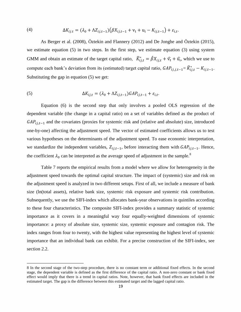
(4) ∆𝐾𝑖𝑗.𝑡 = (𝜆0 + Λ𝑍𝑖𝑗,𝑡−1)(𝛽𝑋𝑖𝑗,𝑡−1 + vt + ui − 𝐾𝑖𝑗,𝑡−1) + 𝜀𝑖,𝑡.

As Berger et al. (2008), Öztekin and Flannery (2012) and De Jonghe and Öztekin (2015),

we estimate equation (5) in two steps. In the first step, we estimate equation (3) using system

GMM and obtain an estimate of the target capital ratio, ��𝑖𝑗,𝑡∗ = ��𝑋𝑖𝑗,𝑡 + vt + ui, which we use to

compute each bank’s deviation from its (estimated) target capital ratio, 𝐺𝐴𝑃𝑖𝑗,𝑗,𝑡−1= ��𝑖𝑗,𝑡∗ −𝐾𝑖𝑗,𝑡−1.

Substituting the gap in equation (5) we get:

(5) ∆𝐾𝑖𝑗,𝑡 = (𝜆0 + Λ𝑍𝑖𝑗,𝑡−1)𝐺𝐴𝑃𝑖𝑗,𝑡−1 + 𝜀𝑖,𝑡.

Equation (6) is the second step that only involves a pooled OLS regression of the

dependent variable (the change in a capital ratio) on a set of variables defined as the product of

𝐺𝐴𝑃𝑖𝑗,𝑡−1 and the covariates (proxies for systemic risk and (relative and absolute) size, introduced

one-by-one) affecting the adjustment speed. The vector of estimated coefficients allows us to test

various hypotheses on the determinants of the adjustment speed. To ease economic interpretation,

we standardize the independent variables, 𝑍𝑖𝑗,𝑡−1, before interacting them with 𝐺𝐴𝑃𝑖𝑗,𝑡−1. Hence,

the coefficient 𝜆0 can be interpreted as the average speed of adjustment in the sample.8

Table 7 reports the empirical results from a model where we allow for heterogeneity in the

adjustment speed towards the optimal capital structure. The impact of (systemic) size and risk on

the adjustment speed is analyzed in two different setups. First of all, we include a measure of bank

size (ln(total assets), relative bank size, systemic risk exposure and systemic risk contribution.

Subsequently, we use the SIFI-index which allocates bank-year observations in quintiles according

to these four characteristics. The composite SIFI-index provides a summary statistic of systemic

importance as it covers in a meaningful way four equally-weighted dimensions of systemic

importance: a proxy of absolute size, systemic size, systemic exposure and contagion risk. The

index ranges from four to twenty, with the highest value representing the highest level of systemic

importance that an individual bank can exhibit. For a precise construction of the SIFI-index, see

section 2.2.

8 In the second stage of the two-step procedure, there is no constant term or additional fixed effects. In the second

stage, the dependent variable is defined as the first difference of the capital ratio. A non-zero constant or bank fixed

effect would imply that there is a trend in capital ratios. Note, however, that bank fixed effects are included in the

estimated target. The gap is the difference between this estimated target and the lagged capital ratio.

20

We report results in three panels, corresponding with the three capital definitions we

employ. However, for each column, the three regressions are estimated as a system of equations

using Seemingly Unrelated Regressions, to account for possible contemporaneous cross-equation

error correlation (see Zellner, 1962). The reported p-values are based on standard errors obtained

via a bootstrap procedure to mitigate issues related to predictor-generated regressors (see Pagan,

1984), as the gap depends on the estimated targets (Faulkender et al., 2012; Çolak et al., 2018).

[Insert Table 7 about here]

In the upper panel, we provide the results for the leverage ratio. In column 1, we report the

homogenous speed of adjustment. In line with previous results, average leverage speed is 0.36.

Thus, on average, banks close 36 percent of the gap between actual and target leverage per year. In

the next column, we introduce jointly the effects of systemic risk and size on leverage speed of

adjustment. We find a positive and statistically significant relationship between ∆CoVaR

(systemic risk contribution) and the speed of adjustment, indicating that banks who impose more

externalities on the system adjust faster. Relative bank size and absolute bank size carry a negative

and statistically significant effect.

These results shed light on two aspects regarding SIFIs and TBTF. As highlighted above,

∆CoVaR apprehends the aggregate financial system performance conditional on a given bank's

returns dropping below a certain threshold. Such a measure is hence expected to capture contagion

risks. Accordingly, banks are more sensitive to adjust their leverage faster when they choose to

take more correlated risks. Although they have access to inexpensive external capital and cheap

debt funding, sizeable banks can, presumably because of their TBTF status, afford to adjust their

leverage ratio more slowly. Such a ratio is indeed not a regulatory risk-based capital measure that

they need to comply with. Such a finding is consistent with moral hazard behavior that leads banks

to take on excessive risk-taking and engage in multiple activities (e.g., combining lending and

trading), when they expect to be bailed out in case of distress. Alternatively, larger banks could be

regarded as more complex and opaque, making it relatively more difficult and costlier for them to

raise capital.

21

The economic effect of a one standard deviation change in absolute and relative size on the

speed of adjustment is slightly larger than that of a similar change in systemic risk contributions.

This is also reflected in column 3, where we use an index of systemic importance and risk. We

find that SIFIs adjust significantly slower towards their target ratio, indicating once more that for

leverage adjustments, the size effect dominates the systemic risk aspect.

In the middle and lower panel, we report results for similar regressions except that we

focus now on regulatory risk weighted capital ratios (Tier 1RWA ratio in middle panel and Total

capital ratio in lower panel). The first column examines the average adjustment. In subsequent

columns, conversely to what we find in the leverage ratio specifications, only the coefficient on

the interaction terms related to the MES is significantly positive, while the effects of ∆CoVaR and

size on speed of adjustment are not significant. Hence, banks with higher MES adjust faster to the

target Tier 1 regulatory ratio.

As there are no opposite effects on the adjustment speed for the various constituents of the

SIFI index, it is not surprising that we find, in column 3, that the systemic index coefficient is

positive and significant, just as for the MES. The result is also economically important and similar

in magnitude for the MES interaction effect. A one standard deviation increase in the index of

systemic importance and risk increases the average Tier1 regulatory adjustment speed by 0.018,

leading to a slightly lower half-life. Such results confirm the hypothesis that SIFIs and TBTF

institutions may find it easier to change their regulatory capital structure by altering the

composition of new equity (Tier1) issuances and adjusting their risky asset compositions, and thus

adjust faster. This is possibly because of higher financial flexibility through relative cost

advantages on the one hand and adjustments in external growth funding on the other hand. The

exposure to common shocks that affect the whole financial system (namely the MES) dominates

the effects of contagion risk and size effects, possibly because banks have to face internally

increased market monitoring and macroprudential regulatory supervision on the one hand and high

expected capital shortfall on the other hand, which translate into higher regulatory adjustment

speed. In addition, it confirms the hypothesis that systemic banks may find it easier to change their

capital structure by raising inexpensive external capital, cheap debt funding and by altering the

asset compositions of their balance sheets.

22

In the lower panel, we repeat the same regressions for the total regulatory capital. All

results are similar to those we obtain for the Tier 1 regulatory ratio in the middle panel. In sum, we

learn that the asymmetry in behavior across capital concepts is driven by different elements of the

SIFI index. First of all, systemic risk and size affect the extent to which banks adjust their capital

ratios. Second, these factors play an opposite role (on the speed of adjustment) for a leverage ratio

vis-à-vis regulatory capital ratios.

4.2. Does regulatory pressure affect (SIFIs’) adjustment speeds?

We find that the speed of adjustment for leverage ratios is faster than that of regulatory

capital ratios. Furthermore, we also find that SIFIs adjust their regulatory capital ratios swifter than

other banks and vice versa for the leverage ratio. In this subsection, we analyze whether these

differences are caused by regulatory pressure. Banks might indeed have less latitude to freely

adjust their regulatory capital ratios and specifically to even a lesser extent when their regulatory

capital buffer is small or when they are below the minimum requirements.

We divide banks in a group of well capitalized banks on the one hand, and banks under

regulatory pressure on the other hand. The group distinction is based on whether or not banks have

both regulatory capital ratios, the Tier1 ratio and the total capital ratio, above the FDICs ‘Well

Capitalized’ levels, 8% and 10% respectively. If they do not meet both thresholds, we classify

them as potentially being under “Regulatory Pressure”. Specifically, we introduce the dummy

variable ‘Regulatory Pressure’ in our model to distinguish the two groups9.

In column 4 of Table 7, we analyze whether banks under regulatory pressure have a different

adjustment speed. In column 5 of Table 7, we interact the SIFI-index and the Regulatory Pressure

variable and investigate their joint impact on adjustment speeds.

9 This dummy variable takes the value of one if a bank’s Tier1 RWA capital ratio falls below 8% and/or its Total

RWA capital ratio falls below 10%. These thresholds coincide with the levels used by the FDIC to determine whether

US banks are well-capitalized or not. Whenever they are not Well Capitalized, various Prompt Corrective Actions

may come into play putting regulatory pressure on adjustment (mechanisms) of bank characteristics. We use the FDIC

thresholds for all banks in the sample in the absence of such information for non-US banks. Recall further, from Table

2, that most banks hold regulatory capital ratios well above the minimum requirements. We are thus mostly

differentiating banks that are well above both regulatory requirements versus banks with small, but positive buffers.

23

First of all, using the dummy variable for being under regulatory pressure or not, we find

that banks that are not in the highest capitalization group (i.e. under regulatory pressure) adjust

slower to the target leverage compared to those who are. The difference is economically large.

This indicates that banks that are not in the most comfortable zone with respect to regulatory

thresholds may indeed not have discretion in their channels of adjustment, which could slow down

the adjustment speed on the leverage ratio. Subsequently, in panels B and C of column 4, we do

not find a significant difference in the adjustment speed for banks under regulatory pressure.

Contrary to what we find for the leverage ratio, the potential lack of discretion that leads to slower

speeds of adjustment for the leverage ratio does not lead to slower speeds of adjustment for the

Tier 1 regulatory ratios. This indicates that the adjustment mechanisms imposed by the regulators

effectively aim at affecting the regulatory capital ratio solely. Finally, in column 5, we do not find

that the interaction effect between the SIFI-index and the dummy variable ‘regulatory pressure” is

significant. Yet, the results documented in columns 3 and 4 pertain.

In sum, the results in Table 7 indicate that banks adjust their regulatory capital ratios

slower than their leverage ratios possibly because they are constrained in their scope by regulation.

In general, they can make faster adjustments to the leverage ratio. The latter are, however, slowed

down when they hold small regulatory capital buffers, because of additional scrutiny and pressure

from regulators.

4.3. Do SIFIs use different adjustment mechanisms?

The analyses thus far indicate that: (i) the mechanisms that banks use to adjust their capital

ratios to return to target depend on whether they are over- or undercapitalized, (ii) the magnitude

of the adjustments vary with the type of capital ratio, (iii) the speed of adjustment depends on the

systemic importance of the bank. These combined insights lead to the last research question, which

is analyzing in a uniform setup whether the adjustment mechanisms differ for SIFIs, depend on the

type of capital ratio and depend on the sign of the capital gap.

To address this question, we estimate the following two threshold regression models:

(7a)

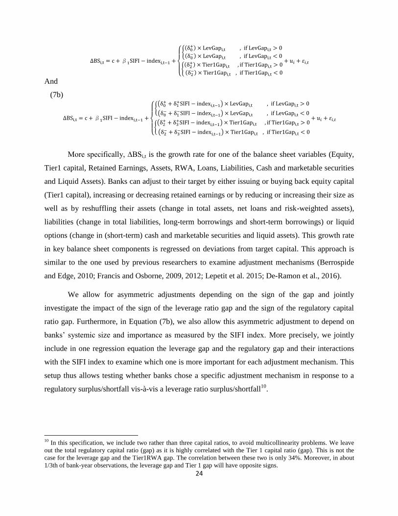
24

∆BSi,t = c +β1SIFI − indexi,t−1 +

{

{(δ0+) × LevGapi,t , if LevGapi,t > 0

(δ0−) × LevGapi,t , if LevGapi,t < 0

{(δ2+) × Tier1Gapi,t , if Tier1Gapi,t > 0

(δ2−) × Tier1Gapi,t , if Tier1Gapi,t < 0

+ 𝑢𝑖 + 𝜀𝑖,𝑡

And

(7b)

∆BSi,t = c +β1SIFI − indexi,t−1 +

{

{(δ0+ + δ1

+SIFI − indexi,t−1) × LevGapi,t , if LevGapi,t > 0

(δ0− + δ1

−SIFI − indexi,t−1) × LevGapi,t , if LevGapi,t < 0

{(δ2+ + δ3

+SIFI − indexi,t−1) × Tier1Gapi,t , if Tier1Gapi,t > 0

(δ2− + δ3

−SIFI − indexi,t−1) × Tier1Gapi,t , if Tier1Gapi,t < 0

+ 𝑢𝑖 + 𝜀𝑖,𝑡

More specifically, ∆BSi,t is the growth rate for one of the balance sheet variables (Equity,

Tier1 capital, Retained Earnings, Assets, RWA, Loans, Liabilities, Cash and marketable securities

and Liquid Assets). Banks can adjust to their target by either issuing or buying back equity capital

(Tier1 capital), increasing or decreasing retained earnings or by reducing or increasing their size as

well as by reshuffling their assets (change in total assets, net loans and risk-weighted assets),

liabilities (change in total liabilities, long-term borrowings and short-term borrowings) or liquid

options (change in (short-term) cash and marketable securities and liquid assets). This growth rate

in key balance sheet components is regressed on deviations from target capital. This approach is

similar to the one used by previous researchers to examine adjustment mechanisms (Berrospide

and Edge, 2010; Francis and Osborne, 2009, 2012; Lepetit et al. 2015; De-Ramon et al., 2016).

We allow for asymmetric adjustments depending on the sign of the gap and jointly

investigate the impact of the sign of the leverage ratio gap and the sign of the regulatory capital

ratio gap. Furthermore, in Equation (7b), we also allow this asymmetric adjustment to depend on

banks’ systemic size and importance as measured by the SIFI index. More precisely, we jointly

include in one regression equation the leverage gap and the regulatory gap and their interactions

with the SIFI index to examine which one is more important for each adjustment mechanism. This

setup thus allows testing whether banks chose a specific adjustment mechanism in response to a

regulatory surplus/shortfall vis-à-vis a leverage ratio surplus/shortfall10

.

10

In this specification, we include two rather than three capital ratios, to avoid multicollinearity problems. We leave

out the total regulatory capital ratio (gap) as it is highly correlated with the Tier 1 capital ratio (gap). This is not the

case for the leverage gap and the Tier1RWA gap. The correlation between these two is only 34%. Moreover, in about

1/3th of bank-year observations, the leverage gap and Tier 1 gap will have opposite signs.

25

In Table 8, we report the results of our estimates of the model presented in equations (7a)

and (7b). The columns correspond with the growth rates in various balance sheet items. The

reported standard errors are obtained via a bootstrap procedure to mitigate issues related to

predictor-generated regressors (see Pagan, 1984), as the gap depends on the estimated targets

(Faulkender et al., 2012; Çolak et al., 2018).

[Insert Table 8 about here]

In panel A, we first report results for the restricted Equation (7a), in which we do not allow

yet for interaction terms between the capital ratio gaps and the SIFI. First of all, the

coefficients associated with the systemic index variable (SIFI-index) are in general significant and

negative, indicating that compared to "less" systemic banks, "more" systemic banks have ceteris

paribus a lower growth rate in total assets but also in the different balance sheet components.

Furthermore, we find that active capital management (growth in equity and Tier 1 capital)

is mainly used when banks are undercapitalized with respect to their own regulatory capital target.

The larger the shortfall of the Tier 1 capital ratio from its target, the larger the growth rate in

equity and Tier 1 capital implying that banks rely on equity issuance. Moreover, the relative

magnitudes of these estimated coefficients is larger for Tier 1 than for common equity indicating

that they prefer other instruments eligible for Tier 1 capital over pure equity in these occasions.

Interestingly and as expected, total asset growth is driven by deviations from the leverage

target, whereas risk-weighted asset growth is driven by regulatory capital deviations. Concerning

total asset growth, we find an economically large effect of a positive leverage gap. The more

undercapitalized a bank is with respect to its leverage target, the larger the reduction in bank size.

Concerning the RWA growth rate, we find that it to be lower, the more the bank’s regulatory

capital ratio falls below its own target. However, when banks are overcapitalized with respect to

their Tier 1 target, the growth rate of RWA is larger, the more they are overcapitalized (i.e., the

more negative the Tier 1 gap becomes). Moreover, the responsiveness of RWA growth to the

magnitude of the gap is larger when they are above their regulatory target capital ratio, than when

they are below.

Regarding liability growth rate, we find it to be affected both by the leverage ratio gap and

the regulatory capital ratio gap, and to a similar extent for both ratios and also irrespective of the

26

sign of the gap. On the one hand, the more banks are undercapitalized (i.e., increases in the

positive gap), the lower is the growth in liabilities. On the other hand, the more banks are

overcapitalized (i.e., decreases in the negative gap), the higher is their liabilities growth rate.

Similarly to liabilities, loan growth is driven by both shortfalls and surpluses of both the leverage

ratio and Tier 1 capital ratio. In terms of economic magnitude, the responsiveness is slightly larger

for the regulatory capital definition.

Finally, cash growth and liquid asset growth is larger when the Tier 1 capital ratio is below

target. The additional Tier 1 capital that undercapitalized banks raise is mainly hoard as cash

(hence the growth), which subsequently reduces the RWA growth. However, when their leverage

ratio is above their target (negative leverage gap), banks reduce their liquid asset growth, which is

in contract to expectations as it harms in closing the gap.

We now turn to the unconstrained Equation (7b). That is, we now investigate the balance

sheet adjustments in response to gaps in the leverage ratio and Tier 1 regulatory capital ratio, also

allowing for heterogeneity depending on the SIFI index and the signs of both the leverage and

regulatory gaps. In panel B of Table 8, we find that the interaction with the SIFI index is more

often significant when banks experience a positive gap (hence capital shortfall) and this both for

the leverage ratio and the Tier 1 capital ratio. The responsiveness of equity, liabilities and asset

growth with respect to shortfalls from the Tier 1 capital target ratio is larger, for a given magnitude

of the shortfall, for SIFIs compared to non-SIFIs. This indicates that for increasingly larger

regulatory capital gaps, compared to smaller banks, SIFIs resort more to raising equity,

downsizing and shrinking debts. On the contrary, SIFIs exhibit a lower responsiveness in

adjustment mechanisms (equity, Tier 1 capital, retained earnings and total assets) when they are

undercapitalized with respect to the leverage ratio target. These findings are consistent with the

idea that banks with capital shortfall have less capacity to grow, lend and/or get into debt

compared with other banks. In all instances, these both sets of results are consistent with the

results in panels of Table 7, where we found a lower adjustment speed for SIFIs for the leverage

ratio and a faster adjustment speed for SIFIs for the regulatory capital ratios than less systemic

institutions.

27

Finally, in panel C, we present an extension of Equation (7b) and also analyze whether

regulatory pressure affects the channels that banks use to adjust their capital ratio towards their

target. First of all, note that adding these additional interaction terms leaves the results on the other

coefficients unaffected. The discussion of the results of panel B thus pertains. Second, we find that

banks that are under regulatory and supervisory pressure, adjust certain items to a different extent

compared to their well-capitalized peers.

Banks under regulatory pressure are found to issue Tier1 capital more extensively, the

more negative the leverage gap becomes. Hence, even though these banks would need lower

equity growth to get back to their leverage target, they possibly make adjustments in line with the

regulatory requirements. Consequently, this will slow down their leverage adjustment speed,

which supports the findings reported in column 4 of panel A of Table 7. Moreover, such banks

reduce their asset growth to a lesser extent for a given leverage shortfall, also in line with the

lower adjustment speed of leverage ratios for banks that are under regulatory pressure. On the

other hand, they reduce their liabilities and loan growth to a larger extent when their leverage ratio

is below their target (when banks are overleveraged).

We now turn to the interaction effects of the Tier1RWA gap and the regulatory pressure

variable. In contrast to the results in rows 5 and 6, we hardly find any significant interaction

coefficients in rows 11 and 12 (except for Cash and marketable securities and Liquid assets)

indicating that the impact of the magnitude and sign of the regulatory capital gap on the

adjustment mechanisms does not differ when banks are under regulatory pressure or not. This lack

of significance squares with the findings presented in panels B and C of Table 7, where we showed

that the speed of adjustment of regulatory capital ratios was not different when banks might be

facing regulatory pressures.

5. Robustness checks and further issues

We examine the robustness of our results to alternative specifications. First, we analyze

two sources of non-linearities in the speed of adjustment. First, we test whether the speed of

adjustment depends on the sign of the gap. Put differently, we allow for asymmetric adjustment

28

speeds for over –and undercapitalized banks. Second, we also test whether the speed of adjustment

of the leverage ratio depends on the stance (sign) of the regulatory capital ratio and vice versa.

These two sources of asymmetries in the speed of adjustment are analyzed in Table 9. In summary,

we show in column 1 of panels A, B and C that the speed of adjustment is significantly lower

when banks are overcapitalized than when they are undercapitalized, but this effect is more

dominant for the leverage ratio than the regulatory capital ratio. Furthermore, in column 2, the

interaction coefficient with the dummy of being undercapitalized with respect to the other capital

concept (i.e., Tier 1 capital gap in panel A, the leverage ratio in panels B and C) is significant in

three occasions and if so, it is negative. In panel A, we find that the asymmetry in adjustment

speed above and below target is exacerbated when banks are undercapitalized in the other capital

dimension, i.e. with respect to their internal target for the regulatory capital ratio. This is not only

an indication that these two capital concepts are not treated in isolation by banks, but also that

banks that are below their regulatory target respond slower. The latter finding could be due to

more regulatory scrutiny (and hence less room for flexibility) when banks' regulatory capital ratios

are lower. Meanwhile, we do not find that the stance of the leverage gap matters for the speed of

adjustment of the regulatory capital ratio.

[Insert Table 9 about here]

Second, De-Ramon et al. (2016) have shown that the balance sheet adjustments that UK

banks make to get back to their target have changed since the global financial crisis. We

investigate a similar issue, but rather than looking at each and every adjustment mechanisms, we

look at the impact on the speed of adjustment, which summarizes the underlying adjustment

mechanism. In particular, we not only check whether the speed of adjustment has changed since

2007, but also whether systemic importance have different effects on the adjustment speed during

the pre-global financial crisis period and during the (post-)crisis period. Indeed, capital

management and balance sheet behavior may be influenced by banks' ability to tap capital

markets. For that purpose, we analyze the impact of systemic importance on adjustment speed

estimations allowing for non-linearity in the relationship by a dummy capturing the normal pre-

crisis times (2001-2006) and crisis and post global financial crisis sample years (2007-2012). In

panel A of Table 10, we report the regression results. In the lower panel B, we present the

29

adjustment speeds implied by the estimated coefficients (by capital ratio definition) for the pre-

and post-2007 period, for small banks, average banks and SIFIs. Small banks (SIFIs) are defined

as those for which the normalized SIFI index is -1 (+1), i.e. one standard deviation below (above)

the mean.

[Insert Table 10 about here]

In this robustness check, we find first of all, that adjustment speeds went up since 2007,

both for small and average banks as well as SIFIs and for all capital ratio definitions. Second, we

find prior to 2007 that SIFIs adjust slower than small banks, with larger differences between the

two groups for leverage ratios compared to regulatory capital ratios. Third, in the post 2007 period,

SIFIs still adjust their leverage ratio slower than small banks, but the difference in adjustment

speeds between the two groups has narrowed compared to the pre-2007 period. Fourth, an opposite

pattern is found for regulatory capital ratios. Since the global financial crisis, the adjustment speed

of regulatory capital ratios has been higher for SIFI banks vis-à-vis small banks. The observation

that SIFIs adjust slower to their leverage capital ratio, and faster to their regulatory capitals ratios,

indicates that SIFIs have become more concerned about their regulatory capital levels than their

leverage since the global financial crisis.

Finally, our sample focuses on banks from 28 OECD countries as these are the countries

where most of the G-SIBs (Globally Systemically Important Banks) are headquartered. One other

country where G-SIBs are prevalent is China. One may wonder whether our results would hold in

the case of the Chinese banking sector which is characterized by a specific institutional

environment. How Chinese banks adjust their capital ratio has been examined by Molyneux et al.

(2014). In particular, they study the role of ownership structure on Chinese banks’ target capital

and speed of adjustment. They do find differences in adjustment speeds depending on ownership

(foreign banks adjust swifter than domestic government-owned banks); but only for regulatory

capital ratios. Furthermore, De Jonghe and Oztekin (2015) report that the speed of adjustment is

slightly lower for mutual institutions (cooperative and savings banks)11

compared with commercial

banks, mostly because they cannot use external capital to make adjustments. Finally, the insights

of De Jonghe and Öztekin (2015) on the cross-country drivers of adjustment speeds shed light on

11

In De Jonghe and Öztekin (2015)’s sample, there are no government owned/connected banks (which would be the

case for China), but the closest resemblance with (Chinese) government-owned banks may be with cooperative and

savings banks who are also not necessarily profit maximizers.

30

whether our results would hold for Chinese SIFIs. While China’s inflation rate is similar to the

average OECD country, its stock market is not yet as developed as in most OECD countries. The

latter may harm swift adjustments in the capital ratio by limiting the possibility to raise equity. As

such, although it could be argued that such banks could easily rely on government capital

injections, we conjecture, but leave it for further research to demonstrate, that SIFIs in China

would, all else equal, have a slower adjustment speed than SIFIs in our sample of banks belonging

to OECD countries.

6. Conclusion

The Basel III Accord has, among other things, introduced more stringent capital

requirements, a new leverage ratio and also capital surcharges for systemically important banks. In

this paper, we investigate how banks adjust their capital ratios to reach their desired levels by

focusing on two dimensions. We look at whether the adjustment speeds and mechanisms are

different for ratios set by regulators (risk-weighted capital ratios) and those internally targeted by

bank managers (leverage) and pay special attention to systemically important banks. We consider

a pre-Basel III period ranging from 2001 and 2012 to examine how banks have managed their

capital ratios by using a sample of listed banks across OECD countries. We augment standard

partial adjustment models of bank capital towards bank-specific and time-varying optimal capital

ratios with various SIFI indicators as well as a systemic risk index based on the quintiles of such

indicators.

On the whole, our findings reveal that the speed at which banks adjust and the way they

adjust show large differences. In general, banks are more flexible and faster in adjusting to their

leverage capital ratio than to regulatory capital ratios. However, SIFIs are slower than other banks

in adjusting to their target leverage ratio but quicker in reaching their target regulatory ratios.

When we dig into the four aspects that define SIFIs, we find that these opposite findings on the

leverage ratio and regulatory ratio are explained by the differential impact that size and systemic

risk have. Larger banks adjust slower and this effect dominates for the leverage ratio, whereas

systemically riskier banks adjust faster and more so their regulatory capital ratios. Furthermore,

banks that are closer to the regulatory minimum requirements are constrained in the adjustments

they can make on their leverage ratio, resulting in a slower speed of adjustment.

31

Our findings contribute to the bank capital structure adjustment literature and carry various

policy implications. In case of any sudden need to augment capital ratios at systemically important

banks, regulators and supervisors should be aware that such institutions would, according to our

results, downsize to a larger extent than smaller banks. If in a given country the market share of

systemic banks is relatively large, the real effects on the economy will consequently be more

important. Symmetrically, a relief in capital constraints or a positive capital shock is also expected

to push SIFIs to expand faster than other banks. On the whole, this procyclical behavior is more

pronounced for systemic institutions, which are however also found to more extensively rely on

equity issues when needed than other banks. Such findings are also expected to be particularly

useful for supervisors when they gauge and adjust the specific capital requirement they can impose

on each bank in the industry differently and separately, which they are allowed to do through Pillar

2 of the Basel III Accord.

Future research could bridge the gap between De Jonghe and Oztekin (2015) and our

paper. They show that the speed of capital structure adjustments by banks is heterogeneous across

countries. In particular, they find that banks make faster capital structure adjustments in countries

with more stringent capital requirements, better supervisory monitoring, more developed capital

markets and high inflation. In our work, we focus instead on heterogeneity in the capital structure

adjustment process across types of banks. An interesting avenue for further research is examining

both issues jointly. That is, one could investigate whether the speed of adjustment differences

between SIFIs and smaller banks are heterogeneous across countries depending on the institutional

setting (e.g., strength of supervision, capital market development) or market structure. The effects

in our sample may be limited as we focus on banks from 28 OECD countries for which the

institutional setting is more homogeneous. A larger cross-country setup could uncover these

potential relationships.

32

Bibliography

Acharya V, Thakor A. (2016) “The dark side of liquidity creation: leverage-induced systemic risk

and implications for the lender of last resort”, Journal of Financial Intermediation, 28, 4–21.

Acharya, V. V., L. H. Pedersen, T. Philippon, and M. P. Richardson (2016) “Measuring Systemic

Risk”, Review of Financial Studies, 30(1), 2–47

Admati, A., P. DeMarzo, M. Hellwig, and P. Pfleiderer (2010) “Fallacies, Irrelevant Facts, and

Myths in the Discussion of Capital Regulation: Why Bank Equity is not Expensive”, Stanford

GSB Research Paper No. 2063.

Adrian, T. and M. K. Brunnermeier (2016) “CoVaR”, American Economic Review, 106(7), 1705–

1741

Adrian, T. and H. S. Shin (2010) “Liquidity and leverage”, Journal of Financial Intermediation,

19(3), 418–437.

Angelini, P., L. Clerc, V. Cúrdia, L. Gambacorta, A. Gerali, A. Locarno, R. Motto, W. Roeger, S.

Van den Heuvel, and J. Vlcek (2011) “Basel III: long-term impact on economic performance and

fluctuations”, Banque de France working paper No. 323.

Barth, A. and Schnabel, I. (2013) “Why banks are not too big to fail - Evidence from the CDS

market”, Economic Policy, 28(74), 335–369.

Baum, C. F., A. Stephan, and O. Talavera (2009) “The effects of uncertainty on the leverage of

nonfinancial firms”, Economic Inquiry, 47 (2), 216–225.

Bertay, A. C., Demirgüç-Kunt, A., and Huizinga, H. (2013) “Do we need big banks? Evidence on

performance, strategy and market discipline”, Journal of Financial Intermediation, 22(4), 532–558.

Berger A, Bouwman C. (2013) “How does capital affect bank performance during financial

crises?”, Journal of Financial Economics, 109 (2013),146–76.

Berger, A., DeYoung, R., Flannery, M., Lee, D., Öztekin, Ö. (2008) “How do large banking

organizations manage their capital ratios?”, Journal of Financial Services Research, 34(2), 123–

149.

Berrospide, J. and R. Edge (2010) “The Effects of Bank Capital on Lending: What Do We Know,

and What Does It Mean?”, International Journal of Central Banking, 6(4), 5–54.

Bhamra, H. S., L. A. Kuehn, and I. A. Strebulaev (2010) “The aggregate dynamics of capital

structure and macroeconomic risk”, Review of Financial Studies, 23 (12), 4187–4241.

Blum, J.M. (2008) “Why basel II may need a leverage ratio restriction”, Journal of Banking and

Finance, 32(8), 1699–1707.

Blundell, R. and S. Bond (1998) “Initial conditions and moment restrictions in dynamic panel data

models”, Journal of Econometrics, 87(1), 115–143.

33

Boyd John H., Stanley L. Graham, R.Shawn Hewitt (1993) “Bank holding company mergers with

nonbank financial firms: Effects on the risk of failure”, Journal of Banking and Finance, 17 (1),

43-63.

Brewer, E., Kaufman, G., Wall, L. (2008) “Bank capital ratios across countries: Why do they

vary?”, Journal of Financial Services Research, 34(2), 177–201.

Brownlees, Christian T., Robert Engle (2012) “Volatility, correlation and tails for

systemic risk measurement”, Working Paper, NYU Stern School of Business.

Brunnermeier, M.K., and L.H. Pedersen (2009) “Market liquidity and funding liquidity”, Review

of Financial Studies, 22(6), 2201–2238.

Byoun, S. (2008) “How and when do firms adjust their capital structures toward targets?”, Journal

of Finance, 63(6), 3069–3096.

Campbell, J.Y., J. Hilscher, J. Szilagyi (2008) “In search of distress risk”, Journal of Finance,

63(6), 2899–2939.

Caglayan, M. and A. Rashid (2014) “The response of firms’ leverage to uncertainty: Evidence

from UK public versus non-public firms”, Economic Inquiry, 52(1), 341–363.

Cecchetti, S. G. (2015) “The Road to Financial Stability: Capital Regulation, Liquidity Regulation,

and Resolution”, International Journal of Central Banking, 11(2), 127–139.

Chen, H. (2010) “Macroeconomic conditions and the puzzles of credit spreads and capital

structure”, Journal of Finance, 65(6), 2171–2212.

Cohen, B. H., and Scatigna, M. (2016) “Banks and capital requirements: Channels of adjustment”,

Journal of Banking and Finance, 69(S1), S56–S69.

Çolak Gönül, Ali Gungoraydinoglu, Özde Öztekin (2018) “Global leverage adjustments,

uncertainty, and country institutional strength”, Journal of Financial Intermediation, 35(A), 41-56.

Cosimano, T.F. and Hakura, D. (2011) “Bank Behavior in Response to Basel III: A Cross-Country

Analysis”, International Monetary Fund Working Paper, 119, 1–34.

De Jonghe, O., Dewachter, H., Mulier, K., Ongena, S. and Schepens, G. (2016) “Some borrowers

are more equal than others: Bank funding shocks and credit reallocation”, Working Paper,

available at SSRN: https://ssrn.com/abstract=2774441.

De Jonghe, O., Öztekin, Ö. (2015) “Bank capital management: International evidence”, Journal of

Financial Intermediation, 24(2), 154–177.

De-Ramon, S. J. and Francis, W. and Harris, Q., (2016) “Bank Capital Requirements and Balance

Sheet Management Practices: “Has the Relationship Changed after the Crisis?”, Bank of England

Working Paper No. 635, available at SSRN: https://ssrn.com/abstract=2885244.

Dermine, J. (2015) “Basel III leverage ratio requirement and the probability of bank runs”, Journal

of Banking and Finance, 53(C), 266–277.

34

Faulkender, M., M. J. Flannery, and J. M. Hankins, K. W.and Smith (2012a) “Cash flows and

leverage adjustments”, Journal of Financial Economics, 103(3), 632–646.

Drobetz, W. and G. Wanzenried (2006) “What determines the speed of adjustment to the target

capital structure?”, Applied Financial Economics, 16 (13), 941–958.

ECB (2007) “Bank capital in Europe and the US. Financial Stability Review”, pp. 155–162.

Farhi E, Tirole J. (2012) “Collective moral hazard, maturity mismatch, and systemic bailouts”,

American Economic Review, 102(1), 60–93.

Faulkender, Michael, Mark J. Flannery, Kristine Watson Hankins, Jason M. Smith (2012) “Cash

flows and leverage adjustments”, Journal of Financial Economics, 103(3), 632-646.

Flannery, M. and K. W. Hankins (2013) “Estimating Dynamic Panel Models in Corporate

Finance”, Journal of Corporate Finance, 19, 1–19.

Flannery, M. and K. Rangan (2006) “Partial adjustment toward target capital structures”, Journal

of Financial Economics, 79(3), 469–506.

Flannery, Mark J. and Kasturi P. Rangan (2006) “Partial adjustment toward target capital

structures”, Journal of Financial Economics, 79(3), 469–506.

Flannery, M.J., and Rangan, K.P. (2008) “What caused the bank capital build-up of the 1990s?”,

Review of Finance, 12(2), 391–429.

Francis, W. and M. Osborne (2012) “Capital requirements and bank behavior in the UK: Are there

lessons for international capital standards?”, Journal of Banking and Finance, 36(3), 803–816.

Giordana, Gaston A., and I. Schumacher (2013) “Bank liquidity risk and monetary policy.

Empirical evidence on the impact of Basel III liquidity standards”, International Review of

Applied Economics, 27(5), 633–55.

Gropp, R. and F. Heider (2010) “The Determinants of Bank Capital Structure”, Review of

Finance, 14(4), 587–622.

Hackbarth, D. Miao, J. and Morellec, E. (2006) “Capital structure, credit risk, and macroeconomic

conditions”, Journal of Financial Economics, 82(3), 519–550.

Harding, J.P., Liang, X., Ross, S.L. (2013) “Bank capital requirements, capital structure and

regulation”, Journal of Financial Services Research 43: 2, pp. 127–148.Hamadi, M., Heinen, A.,

Linder, S., and Porumb, V. A. (2016) “Does Basel II affect the market valuation of discretionary

loan loss provisions?”, Journal of Banking and Finance, 70, 177–92.

Hanson S, Kashyap A, Stein J. (2011) “A macroprudential approach to financial regulation”,

Journal of Economic Perspectives, 25(1), 3–28.

Huang, R., and Ritter, J.R. (2009) “Testing theories of capital structure and estimating the speed of

adjustment”, Journal of Financial and Quantitative Analysis, 44(2), 237–271.

35

Ivashina, V. and D. Scharfstein (2010) “Bank lending during the financial crisis of 2008”, Journal

of Financial Economics, 97(3), 319–338.

Jimenez G. Z., S. Ongena, J. L. Peydró, J. Saurina (2017) “Macroprudential Policy,

countercyclical bank capital buffers and credit supply: Evidence from the Spanish Dynamic

Provisioning Experiments”, Journal of Political Economy, forthcoming.

John K., Kim T., Palia D. (2012) “Heterogeneous Speed of Adjustment in Target Capital

Structure,” Working paper Stern School of Business NYU.

Kiema, I. and E. Jokivuolle (2014) “Does a leverage ratio requirement increase bank stability?”,

Journal of Banking and Finance, 39, 240–254.

Kok, C. and G. Schepens (2013) “Bank reactions after capital shortfalls”, ECB Working Paper No.

1611.

Laeven, Luc, Lev Ratnovski, and Hui Tong (2015) “Bank Size, Capital, and Systemic Risk: Some

International Evidence”, Journal of Banking and Finance, 69 (S1), S25–S34.

Leary, M.T., and Roberts, M.R. (2005) “Do firms rebalance their capital structures?”, Journal of

Finance, 60(6), 2575–2619.

Lemmon, M., Roberts, M. and Zender, J. (2008) “Back to the beginning: Persistence and the cross-

section of corporate capital structure”, Journal of Finance, 63(4), 1575–1608.

Lepetit L., Emmanuelle N., Rous P., Tarazi A. (2008) “Bank income structure and risk: An

empirical analysis of European banks”, Journal of Banking and Finance, 32(8), 1452-1467.

Lepetit, L., Saghi-Zedek N. and Tarazi, A. (2015) “Excess Control Rights, Bank Capital Structure

Adjustments, and Lending”, Journal of Financial Economics, 115(3), 574–591.

Lindquist, K.-G., (2004) “Banks' buffer capital: how important is risk”, Journal of International

Money and Finance 23, 493–513.

Memmel, C., and Raupach, P. (2010) “How do banks adjust their capital ratios?”, Journal of

Financial Intermediation, 19(4), 509–528.

Öztekin, Ö., and Flannery, M.J. (2012) “Institutional determinants of capital structure adjustment

speeds”, Journal of Financial Economics, 103(1), 88–112.

Pagan, Adrian. (1984) “Econometric Issues in the Analysis of Regressions with Generated

Regressors”, International Economic Review, 25(1), 221-247.

Repullo, R. and J. Suarez (2013) “The Procyclical Effect of Bank Capital Regulation”, Review of

Financial Studies, 26(2), 452–490.

Roodman, D (2006) “How to do Xtabond2: an introduction to “Difference” and “System” GMM

in Stata”, Center for Global Development Working Paper 103.

Rubio, M. and Carrasco-Gallego, J.A., (2016), “Coordinating Macroprudential Policies in the Euro

Area: The case of Spain”, Economic Modelling, 59(C), 570–582.

36

Zellner A. (1962) “An Efficient Method of Estimating Seemingly Unrelated Regression Equations

and Tests of Aggregation Bias”, Journal of the American Statistical Association, 57, 500-509.

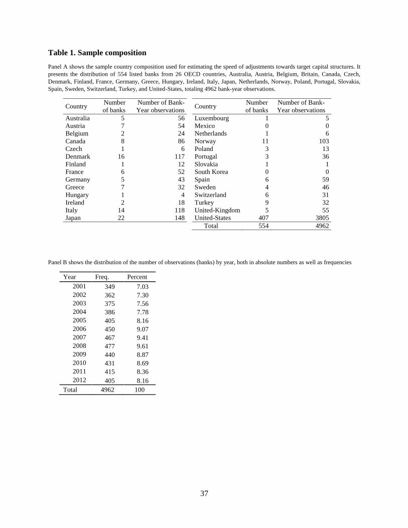
37

Table 1. Sample composition

Panel A shows the sample country composition used for estimating the speed of adjustments towards target capital structures. It

presents the distribution of 554 listed banks from 26 OECD countries, Australia, Austria, Belgium, Britain, Canada, Czech,

Denmark, Finland, France, Germany, Greece, Hungary, Ireland, Italy, Japan, Netherlands, Norway, Poland, Portugal, Slovakia,

Spain, Sweden, Switzerland, Turkey, and United-States, totaling 4962 bank-year observations.

Country Number

of banks

Number of Bank-

Year observations Country

Number

of banks

Number of Bank-

Year observations

Australia 5 56 Luxembourg 1 5

Austria 7 54 Mexico 0 0

Belgium 2 24 Netherlands 1 6

Canada 8 86 Norway 11 103

Czech 1 6 Poland 3 13

Denmark 16 117 Portugal 3 36

Finland 1 12 Slovakia 1 1

France 6 52 South Korea 0 0

Germany 5 43 Spain 6 59

Greece 7 32 Sweden 4 46

Hungary 1 4 Switzerland 6 31

Ireland 2 18 Turkey 9 32

Italy 14 118 United-Kingdom 5 55

Japan 22 148 United-States 407 3805

Total 554 4962

Panel B shows the distribution of the number of observations (banks) by year, both in absolute numbers as well as frequencies

Year Freq. Percent

2001 349 7.03

2002 362 7.30

2003 375 7.56

2004 386 7.78

2005 405 8.16

2006 450 9.07

2007 467 9.41

2008 477 9.61

2009 440 8.87

2010 431 8.69

2011 415 8.36

2012 405 8.16

Total 4962 100

38

Table 2. Descriptive statistics

This table provides the definition and summary statistics for all the regression variables of a sample of 554 publicly listed OECD banks from 2001 to 2012. We report summary

statistics for variables measured at time t. For all variables (in panels A, B and C), we provide number of observations, mean, standard deviation, as well as some percentiles (p5,

p25, median, p75 and p95) for each variable, across all banks and countries.

Variable Definition Source N Mean SD p5 p25 p50 p75 p95

Panel A: Determinants of the target capital structure

Leverage Common equity ratio defined as total equity over total unweighted assets.

Bloomberg, Thomsen-

Reuters Advanced Analytic

(TRAA)

4962 0.093 0.043 0.039 0.069 0.088 0.109 0.162

Tier1RWA Ratio of capital tier1 over to total risk weighted assets. Bloomberg, Bankscope. 4962 0.117 0.036 0.07 0.093 0.111 0.135 0.182

Total capital Ratio of total capital tier1 over to total risk weighted assets. Bloomberg 4962 0.141 0.039 0.102 0.117 0.132 0.155 0.209

Log(Total Assets) Natural logarithm of bank total assets (in USD billion). TRAA 4962 8.151 2.311 5.585 6.401 7.421 9.395 13.1 Credit Risk Loan Loss Provisions over net loans. TRAA 4962 0.007 0.009 0 0.002 0.004 0.008 0.023

Retail Funding Total customer deposit divided by total funding (st borrow+Tot.Cust.Dep). Bloomberg, TRAA 4962 0.897 0.119 0.652 0.863 0.937 0.979 1 Liquidity Net loans over total deposit. TRAA 4962 1.089 0.312 0.583 0.911 1.085 1.259 1.598

Fixed Assets Net fixed assets over total assets. Bloomberg, TRAA 4962 0.016 0.011 0.003 0.009 0.015 0.021 0.036

Diversification Non-interest income over total income. TRAA 4962 0.196 0.109 0.053 0.119 0.175 0.252 0.414 Loan-to-asset Net loans over total assets. TRAA 4962 0.690 0.148 0.44 0.61 0.692 0.775 1

Efficiency Cost income ratio, non-interest expense over total income. TRAA 4962 0.451 0.131 0.249 0.367 0.44 0.528 0.685

RoA Return on assets, defined as the ratio of net income to total assets. TRAA 4962 0.007 0.01 -0.009 0.004 0.008 0.011 0.017 Market Z-score Return-based Z-score Bloomberg, TRAA 4962 3.429 1.874 0.564 2.053 3.331 4.556 6.844

RWA_TA Risk-weighted asset ratio Bloomberg, TRAA 4945 0.738 0.184 0.415 0.632 0.743 0.869 1

Panel B: Determinants of the adjustment speed

MES (%) Marginal Expected Shortfall Appendix Eq. A1 4859 1.692 1.907 -0.417 0.259 1.257 2.601 5.53

∆CoVaR (%) ∆Conditional Value-at-Risk Appendix Eq. A2 4841 1.557 1.743 -1.006 0.405 1.33 2.609 4.721

TAGdp Natural logarithm of bank total assets over GDP. TRAA, OECD stats

Metadata, IMF WEO 4962 0.063 0.197 0 0 0 0.004 0.518

logTA Natural logarithm of bank total assets (in USD billion). TRAA 4962 8.151 2.311 5.585 6.401 7.421 9.395 13.1 SIFI-index aggregated systemic importance index Subsection 4.1.2

Panel C: Growth in adjustment mechanisms

Total Equity Average growth in total equity scaled by average total equity Bloomberg, TRAA 4962 0.081 0.18 -0.159 0.007 0.064 0.143 0.375

Tier1 capital Average growth in Tier1 capital scaled by average total equity Bloomberg, Bankscope. 4945 0.08 0.172 -0.147 0.008 0.061 0.136 0.376

Retained Earnings Average growth in retained earnings by average total equity Bloomberg, Bankscope. 4962 0.023 0.135 -0.192 -0.012 0.04 0.085 0.185 Total Assets Average growth in total assets scaled by average total assets Bloomberg, TRAA. 4962 0.079 0.196 -0.287 0.001 0.066 0.158 0.421

Net Loans Average growth in net loans scaled by average total assets Bloomberg, TRAA. 4962 0.052 0.092 -0.082 -0.004 0.042 0.095 0.224

Risk-Weighted Assets Average growth in risk-weighted assets by average total assets Bloomberg, TRAA. 4945 0.055 0.122 -0.107 -0.006 0.043 0.103 0.251 Total Liabilities Average growth in total liabilities by average total liabilities Bloomberg, TRAA. 4962 0.081 0.124 -0.09 0.006 0.063 0.141 0.305

LT borrowing Average growth in long-term borrowing by average total liabilities Bloomberg, TRAA. 4961 0.009 0.048 -0.056 -0.01 0 0.023 0.094 ST borrowing Average growth in short-term borrowing scaled by average total liabilities Bloomberg, TRAA. 4962 0.003 0.048 -0.074 -0.016 0 0.022 0.083

∆Leverage Change in common equity ratio (percentage) Bloomberg, TRAA. 4962 -0.009 2.506 -3.911 -0.635 -0.016 0.569 3.991

∆Tier1RWA Change in Tier1 capital ratio (percentage) Bloomberg, Bankscope. 4962 0.144 1.713 -2.54 -0.64 0.09 0.84 2.99 ∆Total capital Change in total capital ratio (percentage) Bloomberg, Bankscope. 4962 0.080 1.822 -2.77 -0.78 0.03 0.9 3.05

groLeverage Average growth rates of common equity ratio. Bloomberg, TRAA. 4962 0.025 0.241 -0.328 -0.075 -0.002 0.073 0.482

groTier1RWA Average growth rates of Tier1 capital ratio. Bloomberg, Bankscope. 4962 0.024 0.154 -0.192 -0.056 0.008 0.081 0.31 groTotal capital Average growth rates of total capital ratio. Bloomberg, Bankscope. 4962 0.015 0.131 -0.176 -0.057 0.003 0.07 0.257

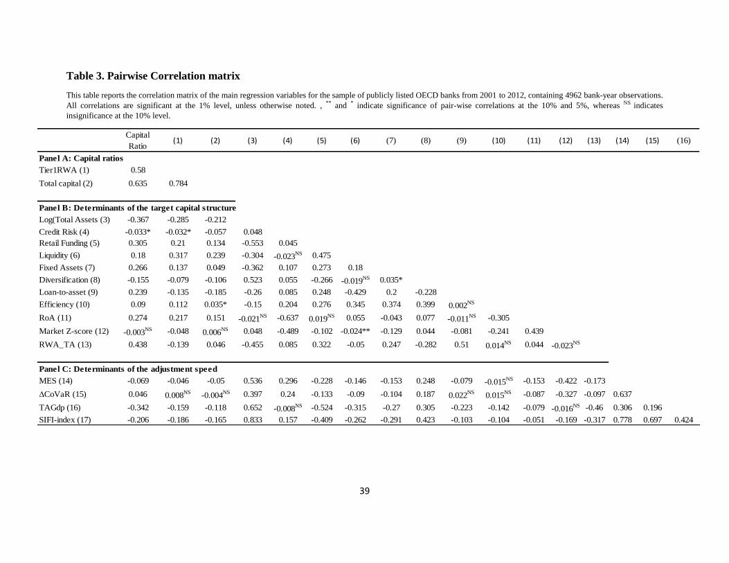
39

Table 3. Pairwise Correlation matrix

This table reports the correlation matrix of the main regression variables for the sample of publicly listed OECD banks from 2001 to 2012, containing 4962 bank-year observations.

All correlations are significant at the 1% level, unless otherwise noted. , ** and * indicate significance of pair-wise correlations at the 10% and 5%, whereas NS indicates

insignificance at the 10% level.

Capital

Ratio(1) (2) (3) (4) (5) (6) (7) (8) (9) (10) (11) (12) (13) (14) (15) (16)

Panel A: Capital ratios

Tier1RWA (1) 0.58

Total capital (2) 0.635 0.784

Panel B: Determinants of the target capital structure

Log(Total Assets (3) -0.367 -0.285 -0.212

Credit Risk (4) -0.033* -0.032* -0.057 0.048

Retail Funding (5) 0.305 0.21 0.134 -0.553 0.045

Liquidity (6) 0.18 0.317 0.239 -0.304 -0.023NS 0.475

Fixed Assets (7) 0.266 0.137 0.049 -0.362 0.107 0.273 0.18

Diversification (8) -0.155 -0.079 -0.106 0.523 0.055 -0.266 -0.019NS 0.035*

Loan-to-asset (9) 0.239 -0.135 -0.185 -0.26 0.085 0.248 -0.429 0.2 -0.228

Efficiency (10) 0.09 0.112 0.035* -0.15 0.204 0.276 0.345 0.374 0.399 0.002NS

RoA (11) 0.274 0.217 0.151 -0.021NS -0.637 0.019

NS 0.055 -0.043 0.077 -0.011NS -0.305

Market Z-score (12) -0.003NS -0.048 0.006

NS 0.048 -0.489 -0.102 -0.024** -0.129 0.044 -0.081 -0.241 0.439

RWA_TA (13) 0.438 -0.139 0.046 -0.455 0.085 0.322 -0.05 0.247 -0.282 0.51 0.014NS 0.044 -0.023

NS

Panel C: Determinants of the adjustment speed

MES (14) -0.069 -0.046 -0.05 0.536 0.296 -0.228 -0.146 -0.153 0.248 -0.079 -0.015NS -0.153 -0.422 -0.173

∆CoVaR (15) 0.046 0.008NS

-0.004NS 0.397 0.24 -0.133 -0.09 -0.104 0.187 0.022

NS0.015

NS -0.087 -0.327 -0.097 0.637

TAGdp (16) -0.342 -0.159 -0.118 0.652 -0.008NS -0.524 -0.315 -0.27 0.305 -0.223 -0.142 -0.079 -0.016

NS -0.46 0.306 0.196

SIFI-index (17) -0.206 -0.186 -0.165 0.833 0.157 -0.409 -0.262 -0.291 0.423 -0.103 -0.104 -0.051 -0.169 -0.317 0.778 0.697 0.424

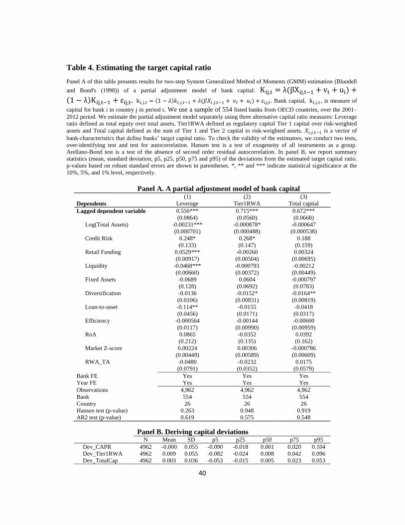
40

Table 4. Estimating the target capital ratio

Panel A of this table presents results for two-step System Generalized Method of Moments (GMM) estimation (Blundell

and Bond's (1998)) of a partial adjustment model of bank capital: Kij,t = λ(βXij,t−1 + vt + ui) +

(1 − λ)Kij,t−1 + εij,t. k𝑖,𝑗,𝑡 = (1 − 𝜆)𝑘𝑖,𝑗,𝑡−1 + 𝜆(𝛽𝑋𝑖,𝑗,𝑡−1 + 𝑣𝑡 + u𝑖) + εi,j,t. Bank capital, k𝑖,𝑗,𝑡, is measure of

capital for bank i in country j in period t. We use a sample of 554 listed banks from OECD countries, over the 2001–

2012 period. We estimate the partial adjustment model separately using three alternative capital ratio measures: Leverage

ratio defined as total equity over total assets, Tier1RWA defined as regulatory capital Tier 1 capital over risk-weighted

assets and Total capital defined as the sum of Tier 1 and Tier 2 capital to risk-weighted assets. 𝑋𝑖,𝑗,𝑡−1 is a vector of

bank-characteristics that define banks’ target capital ratio. To check the validity of the estimators, we conduct two tests,

over-identifying test and test for autocorrelation. Hansen test is a test of exogeneity of all instruments as a group.

Arellano-Bond test is a test of the absence of second order residual autocorrelation. In panel B, we report summary

statistics (mean, standard deviation, p5, p25, p50, p75 and p95) of the deviations from the estimated target capital ratio.

p-values based on robust standard errors are shown in parentheses. *, ** and *** indicate statistical significance at the

10%, 5%, and 1% level, respectively.

Panel A. A partial adjustment model of bank capital (1) (2) (3)

Dependents Leverage Tier1RWA Total capital

Lagged dependent variable 0.556*** 0.715*** 0.672***

(0.0864) (0.0560) (0.0668)

Log(Total Assets) -0.00231*** -0.000878* -0.000647

(0.000701) (0.000488) (0.000538)

Credit Risk 0.248* 0.268* 0.188

(0.133) (0.147) (0.159)

Retail Funding 0.0529*** -0.00260 0.00324

(0.00917) (0.00504) (0.00695)

Liquidity -0.0468*** -0.000793 -0.00212

(0.00660) (0.00372) (0.00449)

Fixed Assets -0.0689 0.0604 -0.000797

(0.128) (0.0692) (0.0783)

Diversification -0.0136 -0.0152* -0.0164**

(0.0106) (0.00831) (0.00819)

Loan-to-asset -0.114** -0.0155 -0.0418

(0.0456) (0.0171) (0.0317)

Efficiency -0.000564 -0.00144 -0.00600

(0.0117) (0.00990) (0.00959)

RoA 0.0865 -0.0352 0.0392

(0.212) (0.135) (0.162)

Market Z-score 0.00224 0.00306 -0.000786

(0.00449) (0.00589) (0.00609)

RWA_TA -0.0480 -0.0232 0.0175

(0.0791) (0.0352) (0.0579)

Bank FE Yes Yes Yes

Year FE Yes Yes Yes

Observations 4,962 4,962 4,962

Bank 554 554 554

Country 26 26 26

Hansen test (p-value) 0.263 0.948 0.919

AR2 test (p-value) 0.619 0.575 0.548

Panel B. Deriving capital deviations N Mean SD p5 p25 p50 p75 p95

Dev_CAPR 4962 -0.000 0.055 -0.090 -0.018 0.001 0.020 0.104

Dev_Tier1RWA 4962 0.009 0.055 -0.082 -0.024 0.008 0.042 0.096

Dev_TotalCap 4962 0.003 0.036 -0.053 -0.015 0.005 0.023 0.053

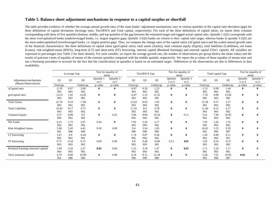
41

Table 5. Balance sheet adjustment mechanisms in response to a capital surplus or shortfall

The table provides evidence of whether the average annual growth rates of the main banks’ adjustment mechanisms vary in various quintiles of the capital ratio deviation (gap) for

three definitions of capital deviations (leverage ratio, Tier1RWA and Total capital, respectively). For each of the three definitions of capital ratios, we report three columns

corresponding with three of five quintiles (bottom, middle, and top quintile) of the gap between the estimated target and lagged actual capital ratio. Quintile 1 (Q1) corresponds with

the most overcapitalized banks (underleveraged banks, i.e. largest negative gap), Quintile 3 (Q3) banks are closest to their capital ratio target, whereas banks in quintile 5 (Q5) are

the most undercapitalized (overleveraged banks, i.e. largest positive gap). Thus, we compare the change rates of the capital ratios (∆Capital ratio) and the scaled annual growth rates

of the financial characteristics: the three definitions of capital ratios (groCapital ratio), total assets (Assets), total common equity (Equity), total liabilities (Liabilities), net loans

(Loans), risk-weighted-assets (RWA), long-term (LT) and short-term (ST) borrowing, internal capital (Retained Earnings) and external capital (Tier1 capital). All variables are

expressed in percentages (see Table 2 for more details). For each variable, we report the average growth rate, the number of observations per group (below the mean value) and the

results of pairwise t-tests of equality of means of the extreme quintiles compared with the middle quintile, respectively. We report the p-values of these equality of means tests and

use a bootstrap procedure to account for the fact that the classificiation in quintiles is based on an estimated target.. Differences in the observations are due to differences in data

availability.

Leverage Gap

Test for equality of

mean

Tier1RWA Gap Test for equality of

mean

Total capital Gap Test for equality of

mean

Adjustment mechanisms

(Means/Observations)

Q1 Q3 Q5

Quintile 1 vs 3

Quintile 3 vs 5

Q1 Q3 Q5 Quintile 1 vs 3

Quintile 3 vs 5

Q1 Q3 Q5 Quintile 1 vs 3

Quintile 3 vs 5

Overcap. Undercap. p-value p-value

Overcap. Undercap. p-value p-value

Overcap. Undercap. p-value p-value

∆Capital ratio -2.19 0.07 2.08 0 0 -0.97 0.18 1.23 0 0 -1.31 0.09 1.44 0 0

993 993 992 993 993 992 993 993 992 groCapital ratio -14.51 1.62 23.65 0 0 -6.47 2.13 12.52 0 0 -7.35 0.89 12.06 0 0

993 993 992 993 993 992 993 993 992

Total Assets 21.78 8.19 -7.69 0 0

12.62 8.02 1.95 0 0

12.58 8.17 2.37 0 0

993 993 992

993 993 992

993 993 992

Total Liabilities 10.43 8.17 4.73 0 0

11.35 8.4 4.78 0 0

11.46 8.12 4.17 0 0

993 993 992

993 993 992

993 993 992

Common Equity 4.37 8.89 9.9 0 0.25 5.96 8.89 10.24 0 0.11 5.61 7.96 10.95 0 0

993 993 992 993 993 992 993 993 992

Net Loans 6.25 5.75 2.87 0.24 0

7.92 5.56 2.17 0 0

7.95 5.26 1.76 0 0

993 993 992

993 993 992

993 993 992

Risk-Weighted Assets 5.96 5.43 4.41 0.30 0.09

9.4 5.54 1.83 0 0

10.62 5.25 0.29 0 0

991 988 990

990 990 989

992 990 987

LT borrowing 1.87 0.9 -0.42 0 0

1.74 0.87 0.26 0 0

1.58 0.89 0.11 0 0

992 993 992

993 993 991

993 993 991 ST borrowing 0.71 0.34 0.15 0.09 0.40

0.8 0.46 -0.68 0.12 010

1.02 0.33 -0.57 0 0

993 993 992

993 993 992

993 993 992

Retained Earnings (internal capital) 1.09 2.56 2.27 0.02 0.64 1.53 3.18 1.47 0 0.01 1.71 3.24 1.17 0 0

993 993 992 993 993 992 993 993 992

Tier1 (external capital) 4.79 8.60 10.09 0 0.08 4.19 8.11 12.18 0 0 5.58 7.61 10.95 0.01 0

991 988 990 990 990 989 992 990 987

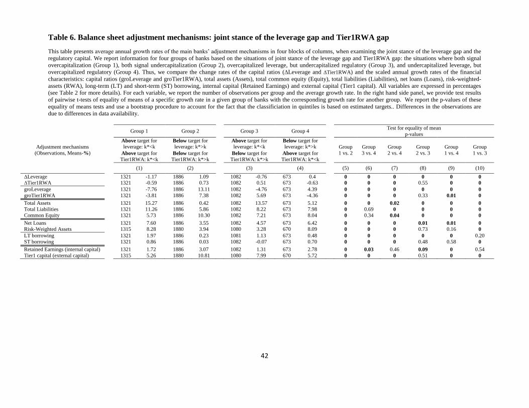
42

Table 6. Balance sheet adjustment mechanisms: joint stance of the leverage gap and Tier1RWA gap

This table presents average annual growth rates of the main banks’ adjustment mechanisms in four blocks of columns, when examining the joint stance of the leverage gap and the

regulatory capital. We report information for four groups of banks based on the situations of joint stance of the leverage gap and Tier1RWA gap: the situations where both signal

overcapitalization (Group 1), both signal undercapitalization (Group 2), overcapitalized leverage, but undercapitalized regulatory (Group 3), and undercapitalized leverage, but

overcapitalized regulatory (Group 4). Thus, we compare the change rates of the capital ratios (∆Leverage and ∆Tier1RWA) and the scaled annual growth rates of the financial

characteristics: capital ratios (groLeverage and groTier1RWA), total assets (Assets), total common equity (Equity), total liabilities (Liabilities), net loans (Loans), risk-weighted-

assets (RWA), long-term (LT) and short-term (ST) borrowing, internal capital (Retained Earnings) and external capital (Tier1 capital). All variables are expressed in percentages

(see Table 2 for more details). For each variable, we report the number of observations per group and the average growth rate. In the right hand side panel, we provide test results

of pairwise t-tests of equality of means of a specific growth rate in a given group of banks with the corresponding growth rate for another group. We report the p-values of these

equality of means tests and use a bootstrap procedure to account for the fact that the classificiation in quintiles is based on estimated targets.. Differences in the observations are

due to differences in data availability.

Group 1 Group 2

Group 3 Group 4

Test for equality of mean

p-values

Adjustment mechanisms

(Observations, Means-%)

Above target for leverage: k*<k

Below target for leverage: k*>k

Above target for leverage: k*<k

Below target for leverage: k*>k

Group

1 vs. 2

Group

3 vs. 4

Group

2 vs. 4

Group

2 vs. 3

Group

1 vs. 4

Group

1 vs. 3 Above target for

Tier1RWA: k*<k

Below target for

Tier1RWA: k*>k

Below target for

Tier1RWA: k*>k

Above target for

Tier1RWA: k*<k

(1) (2) (3) (4) (5) (6) (7) (8) (9) (10)

∆Leverage 1321 -1.17 1886 1.09 1082 -0.76 673 0.4 0 0 0 0 0 0

∆Tier1RWA 1321 -0.59 1886 0.73 1082 0.51 673 -0.63 0 0 0 0.55 0 0

groLeverage 1321 -7.76 1886 13.11 1082 -4.76 673 4.39 0 0 0 0 0 0

groTier1RWA 1321 -3.81 1886 7.38 1082 5.69 673 -4.36 0 0 0 0.33 0.01 0

Total Assets 1321 15.27 1886 0.42 1082 13.57 673 5.12 0 0 0.02 0 0 0

Total Liabilities 1321 11.26 1886 5.86 1082 8.22 673 7.98 0 0.69 0 0 0 0

Common Equity 1321 5.73 1886 10.30 1082 7.21 673 8.04 0 0.34 0.04 0 0 0

Net Loans 1321 7.60 1886 3.55

1082 4.57 673 6.42 0 0 0 0.01 0.01 0

Risk-Weighted Assets 1315 8.28 1880 3.94

1080 3.28 670 8.09 0 0 0 0.73 0.16 0

LT borrowing 1321 1.97 1886 0.23

1081 1.13 673 0.48 0 0 0 0 0 0.20

ST borrowing 1321 0.86 1886 0.03

1082 -0.07 673 0.70 0 0 0 0.48 0.58 0

Retained Earnings (internal capital) 1321 1.72 1886 3.07 1082 1.31 673 2.78 0 0.03 0.46 0.09 0 0.54

Tier1 capital (external capital) 1315 5.26 1880 10.81 1080 7.99 670 5.72 0 0 0 0.51 0 0

43

Table 7: Determinants of adjustment speed to target capital structure: effects of systemic risk and size

on speed of adjustment.

This table reports coefficient estimates for a system of Seeming Unrelated regressions. In particular, we estimate a heterogeneous partial

adjustment model for three different definitions of the capital ratio (Leverage, Tier1RWA and Total capital): k𝑖,j,𝑡 − k𝑖,j,𝑡−1 = (𝜆0 + Λ 𝑍𝑖𝑗,𝑡−1) ×

Gap𝑖,𝑗,𝑡−1+εi,j,t.

The dependent variable is the change in the capital ratio, which is regressed on the gap (deviation between the estimated target and the lagged

value of the capital ratio) and interactions of the gap with other variables captured by 𝑍𝑖𝑗,𝑡−1. In column 2, we include as interaction variables: the

marginal expected shortfall (MES), the delta Conditional Value-at-Risk (∆CoVaR), the relative bank size to GDP (RelativeSize) and the natural

logarithm of bank total assets (Size). In column 3, we use a composite indicator of these four dimensions, labelled SIFI-index. In Column 4, we

add an interaction of the gap with an indicator that is one if either the Tier 1 RWA is below 8% or the Total Capital Ratio is below 10% (not Well-

Capitalized), whereas in the last column we add the composite SIFI index and the Well Capitalized dummy jointly (as well as their interaction).

All continuous variables are standardized before being interacted with the capital deviation to facilitate the economic magnitude interpretation.

The regression results are based on a sample of listed OECD banks over the 2001-2012 period. P-values based on robust standard errors, are

obtained following a bootstrapping procedure to account for the estimated regressors (namely, estimated capital targets are used to obtain the

gaps). Coefficients significantly different from zero at the 1%, 5% and 10% level are marked with ***/**/*. The letter a (b) following the p-values

indicates the cases where that coefficient is significantly different from its analogue in panel a (b) at least at the 10% significance level.

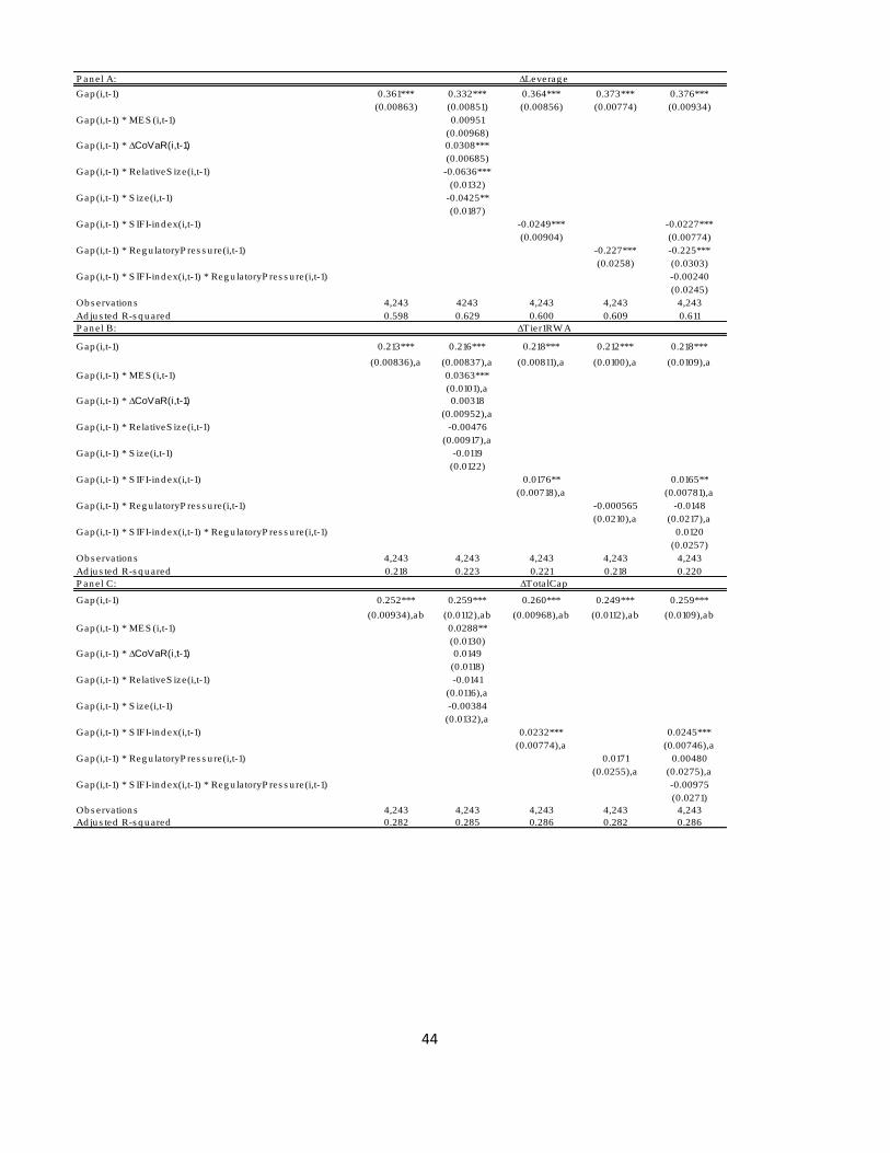
44

P an el A:

Gap (i,t-1) 0.361*** 0.332*** 0.364*** 0.373*** 0.376***

(0.00863) (0.00851) (0.00856) (0.00774) (0.00934)

Gap (i,t-1) * MES (i,t-1) 0.00951

(0.00968)

Gap (i,t-1) * ∆CoVaR(i,t-1) 0.0308***

(0.00685)

Gap (i,t-1) * RelativeS ize(i,t-1) -0.0636***

(0.0132)

Gap (i,t-1) * S ize(i,t-1) -0.0425**

(0.0187)

Gap (i,t-1) * S IFI-in d ex(i,t-1) -0.0249*** -0.0227***

(0.00904) (0.00774)

Gap (i,t-1) * Reg u latoryP res s u re(i,t-1) -0.227*** -0.225***

(0.0258) (0.0303)

Gap (i,t-1) * S IFI-in d ex(i,t-1) * Reg u latoryP res s u re(i,t-1) -0.00240

(0.0245)

Ob s ervation s 4,243 4243 4,243 4,243 4,243

Ad ju s ted R-s q u ared 0.598 0.629 0.600 0.609 0.611

P an el B:

Gap (i,t-1) 0.213*** 0.216*** 0.218*** 0.212*** 0.218***

(0.00836),a (0.00837),a (0.00811),a (0.0100),a (0.0109),a

Gap (i,t-1) * MES (i,t-1) 0.0363***

(0.0101),a

Gap (i,t-1) * ∆CoVaR(i,t-1) 0.00318

(0.00952),a

Gap (i,t-1) * RelativeS ize(i,t-1) -0.00476

(0.00917),a

Gap (i,t-1) * S ize(i,t-1) -0.0119

(0.0122)

Gap (i,t-1) * S IFI-in d ex(i,t-1) 0.0176** 0.0165**

(0.00718),a (0.00781),a

Gap (i,t-1) * Reg u latoryP res s u re(i,t-1) -0.000565 -0.0148

(0.0210),a (0.0217),a

Gap (i,t-1) * S IFI-in d ex(i,t-1) * Reg u latoryP res s u re(i,t-1) 0.0120

(0.0257)

Ob s ervation s 4,243 4,243 4,243 4,243 4,243

Ad ju s ted R-s q u ared 0.218 0.223 0.221 0.218 0.220

P an el C:

Gap (i,t-1) 0.252*** 0.259*** 0.260*** 0.249*** 0.259***

(0.00934),ab (0.0112),ab (0.00968),ab (0.0112),ab (0.0109),ab

Gap (i,t-1) * MES (i,t-1) 0.0288**

(0.0130)

Gap (i,t-1) * ∆CoVaR(i,t-1) 0.0149

(0.0118)

Gap (i,t-1) * RelativeS ize(i,t-1) -0.0141

(0.0116),a

Gap (i,t-1) * S ize(i,t-1) -0.00384

(0.0132),a

Gap (i,t-1) * S IFI-in d ex(i,t-1) 0.0232*** 0.0245***

(0.00774),a (0.00746),a

Gap (i,t-1) * Reg u latoryP res s u re(i,t-1) 0.0171 0.00480

(0.0255),a (0.0275),a

Gap (i,t-1) * S IFI-in d ex(i,t-1) * Reg u latoryP res s u re(i,t-1) -0.00975

(0.0271)

Ob s ervation s 4,243 4,243 4,243 4,243 4,243

Ad ju s ted R-s q u ared 0.282 0.285 0.286 0.282 0.286

∆Leverag e

∆Tier1RW A

∆TotalCap

45

Table 8: Balance sheet adjustments by SIFIs: leverage or regulatory driven?

This table reports the coefficient estimates for the regression model (7a) in panel A and regression model (7b) in panel B. In panel C, we report an extension of regression model (7b).

Using a sample of listed OECD banks over the 2001-2012 period, we assess the relation between the annual growth rates of diverse balance sheet items and their capital shortfall (positive

gap, undercapitalized) or their capital surplus (negative gap, overcapitalized) vis-à-vis its target capital ratio. We jointly assess the impact of deviation from the leverage target and the

regulatory capital target ratio. Across columns, the specification is identical except for the dependent variable, which is respectively the average annual growth rates of total common equity

(Equity), Tier1 capital, retained earnings, total assets (Assets), risk-weighted assets (RWA), net loans (Loans), total liabilities (Liabilities), Cash and marketable securities and Liquid

Assets. Growth rates variables are scaled by average total equity, total assets and total liabilities. The gap is computed using two definitions of capital ratio (Leverage and Tier1RWA).

SIFI-indexi,t−1 is an aggregate systemic risk index constructed based on the quintiles of the MES, ∆CoVaR, relative size and size. All regressions include a constant term. P-values based on

robust standard errors, are obtained following a bootstrapping procedure to account for the estimated regressors (namely, estimated capital targets are used to obtain the gaps). *, ** and***

indicate statistical significance at the 10%, 5% and 1% levels respectively. The letter y following the p-values indicates the cases where that coefficient is significantly different at the 10%

significance level from its analogue (with the other capital definition) in the same panel in the same column.

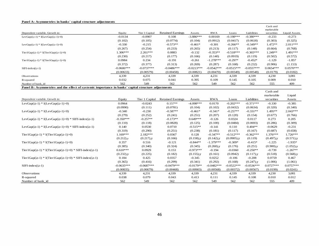
46

Panel A: Asymmetries in banks' capital structure adjustments

Dependent variable. Growth in: Equity Tier 1 Capital Retained Earnings Assets RWA Loans Liabilities

Cash and

marketable

securities Liquid Assets

LevGap(i,t-1) * I(LevGap(i,t-1)>0) -0.0134 -0.0907 0.108 -3.886*** 0.00169 -0.198*** -0.380*** -0.233 -0.273

(0.102) (0.105) (0.0774) (0.104) (0.0912) (0.0417) (0.0618) (0.303) (0.325)

LevGap(i,t-1) * I(LevGap(i,t-1)<0) -0.330 -0.215 -0.573** -0.461* -0.301 -0.266** -0.349** 1.472** 2.011***

(0.267) (0.254) (0.233) (0.265) (0.213) (0.117) (0.148) (0.664) (0.768)

Tier1Gap(i,t-1) * I(Tier1Gap(i,t-1)>0) 1.306*** 2.261*** 0.0883 -0.132 -0.353** -0.518*** -0.365*** 1.249** 1.491***

(0.230) (0.217) (0.177) (0.166) (0.140) (0.0919) (0.119) (0.502) (0.572)

Tier1Gap(i,t-1) * I(Tier1Gap(i,t-1)<0) 0.0984 0.234 -0.191 -0.261 -1.278*** -0.297* -0.452* -1.129 -1.857

(0.372) (0.377) (0.313) (0.269) (0.287) (0.168) (0.232) (0.906) (1.153)

SIFI-index(i,t-1) -0.0606*** -0.0737*** -0.0486*** -0.0213*** -0.0542*** -0.0515*** -0.0557*** 0.0654*** 0.0570***

(0.00633) (0.00579) (0.00458) (0.00821) (0.00470) (0.00349) (0.00548) (0.0179) (0.0182)

Observations 4,339 4,231 4,339 4,339 4,231 4,339 4,339 4,230 3,081

R-squared 0.032 0.075 0.041 0.395 0.109 0.145 0.105 0.009 0.010

Number of bank_id 562 549 562 562 549 562 562 555 409

Panel B: Asymmetries and the effect of systemic importance in banks' capital structure adjustments

Dependent variable. Growth in: Equity Tier 1 Capital Retained Earnings Assets RWA Loans Liabilities

Cash and

marketable

securities

Liquid

Assets

LevGap(i,t-1) * I(LevGap(i,t-1)>0) 0.0964 -0.0243 0.157** -4.098*** 0.0170 -0.202*** -0.371*** -0.330 -0.385

(0.0990) (0.111) (0.0781) (0.104) (0.102) (0.0432) (0.0634) (0.320) (0.340)

LevGap(i,t-1) * I(LevGap(i,t-1)<0) -0.340 -0.230 -0.587** -0.461* -0.341* -0.257** -0.331** 1.495** 2.043***

(0.279) (0.252) (0.241) (0.251) (0.207) (0.120) (0.154) (0.677) (0.766)

LevGap(i,t-1) * I(LevGap(i,t-1)>0) * SIFI-index(i,t-1) -0.350*** -0.257** -0.173** 0.649*** -0.126 0.0324 0.0117 0.273 0.205

(0.110) (0.118) (0.0828) (0.125) (0.100) (0.0484) (0.0693) (0.286) (0.309)

LevGap(i,t-1) * I(LevGap(i,t-1)<0) * SIFI-index(i,t-1) 0.140 0.0530 0.0710 -0.515** -0.141 0.110 0.404** -0.0629 -0.231

(0.319) (0.290) (0.251) (0.238) (0.181) (0.117) (0.167) (0.687) (0.658)

Tier1Gap(i,t-1) * I(Tier1Gap(i,t-1)>0) 1.169*** 2.182*** 0.0367 0.128 -0.347** -0.512*** -0.362*** 1.376*** 1.726***

(0.212),y (0.217),y (0.166) (0.158),y (0.142),y (0.0905),y (0.119) (0.497),y (0.571),y

Tier1Gap(i,t-1) * I(Tier1Gap(i,t-1)<0) 0.357 0.516 -0.121 -0.844** -1.379*** -0.309* -0.415* -1.225 -1.935*

(0.385) (0.340) (0.324) (0.345) (0.260),y (0.176) (0.251) (0.900),y (1.052),y

Tier1Gap(i,t-1) * I(Tier1Gap(i,t-1)>0) * SIFI-index(i,t-1) 0.610*** 0.0929 0.153 -0.973*** -0.194 -0.0360 -0.250** -0.739 -1.267**

(0.232),y (0.225) (0.182) (0.155),y (0.161) (0.0942) (0.117),y (0.518) (0.568),y

Tier1Gap(i,t-1) * I(Tier1Gap(i,t-1)<0) * SIFI-index(i,t-1) 0.184 0.425 0.0357 -0.345 0.0252 -0.106 -0.208 0.0759 0.467

(0.365) (0.416) (0.299) (0.341) (0.292) (0.168) (0.247),y (1.006) (1.061)

SIFI-index(i,t-1) -0.0635*** -0.0687*** -0.0479*** -0.0179** -0.0482*** -0.0522*** -0.0536*** 0.0727*** 0.0757***

(0.00835) (0.00679) (0.00468) (0.00903) (0.00568) (0.00372) (0.00567) (0.0199) (0.0241)

Observations 4,339 4,231 4,339 4,339 4,231 4,339 4,339 4,230 3,081

R-squared 0.038 0.079 0.043 0.413 0.111 0.145 0.108 0.010 0.012

Number of bank_id 562 549 562 562 549 562 562 555 409

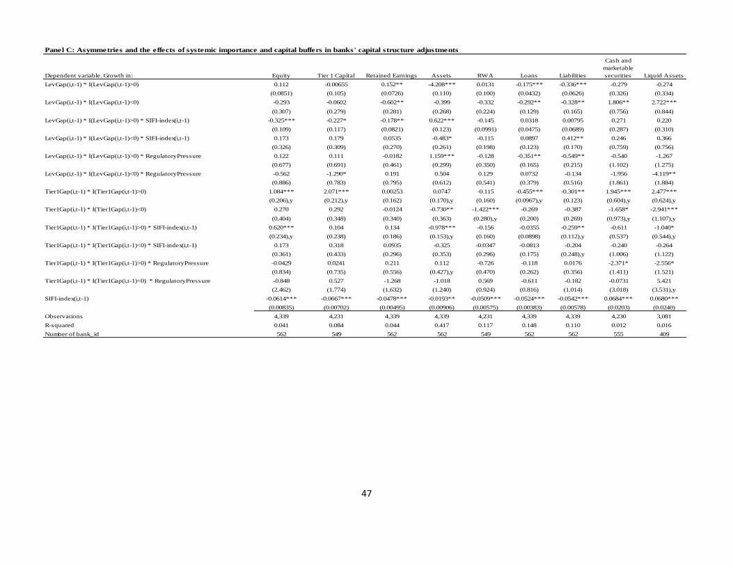
47

Panel C: Asymmetries and the effects of systemic importance and capital buffers in banks' capital structure adjustments

Dependent variable. Growth in: Equity Tier 1 Capital Retained Earnings Assets RWA Loans Liabilities

Cash and

marketable

securities Liquid Assets

LevGap(i,t-1) * I(LevGap(i,t-1)>0) 0.112 -0.00655 0.152** -4.208*** 0.0131 -0.175*** -0.336*** -0.279 -0.274

(0.0851) (0.105) (0.0726) (0.110) (0.100) (0.0432) (0.0626) (0.326) (0.334)

LevGap(i,t-1) * I(LevGap(i,t-1)<0) -0.293 -0.0602 -0.602** -0.399 -0.332 -0.292** -0.328** 1.806** 2.722***

(0.307) (0.279) (0.281) (0.268) (0.224) (0.129) (0.165) (0.756) (0.844)

LevGap(i,t-1) * I(LevGap(i,t-1)>0) * SIFI-index(i,t-1) -0.325*** -0.227* -0.178** 0.622*** -0.145 0.0318 0.00795 0.271 0.220

(0.109) (0.117) (0.0821) (0.123) (0.0991) (0.0475) (0.0689) (0.287) (0.310)

LevGap(i,t-1) * I(LevGap(i,t-1)<0) * SIFI-index(i,t-1) 0.173 0.179 0.0535 -0.483* -0.115 0.0897 0.412** 0.246 0.366

(0.326) (0.309) (0.270) (0.261) (0.198) (0.123) (0.170) (0.759) (0.756)

LevGap(i,t-1) * I(LevGap(i,t-1)>0) * RegulatoryPressure 0.122 0.111 -0.0182 1.159*** -0.128 -0.351** -0.549** -0.540 -1.267

(0.677) (0.691) (0.461) (0.299) (0.350) (0.165) (0.215) (1.102) (1.275)

LevGap(i,t-1) * I(LevGap(i,t-1)<0) * RegulatoryPressure -0.562 -1.290* 0.191 0.504 0.129 0.0732 -0.134 -1.956 -4.119**

(0.886) (0.783) (0.795) (0.612) (0.541) (0.379) (0.516) (1.861) (1.884)

Tier1Gap(i,t-1) * I(Tier1Gap(i,t-1)>0) 1.084*** 2.071*** 0.00253 0.0747 -0.115 -0.455*** -0.301** 1.945*** 2.477***

(0.206),y (0.212),y (0.162) (0.170),y (0.160) (0.0967),y (0.123) (0.604),y (0.624),y

Tier1Gap(i,t-1) * I(Tier1Gap(i,t-1)<0) 0.270 0.292 -0.0124 -0.730** -1.422*** -0.269 -0.387 -1.658* -2.941***

(0.404) (0.348) (0.340) (0.363) (0.280),y (0.200) (0.269) (0.973),y (1.107),y

Tier1Gap(i,t-1) * I(Tier1Gap(i,t-1)>0) * SIFI-index(i,t-1) 0.620*** 0.104 0.134 -0.978*** -0.156 -0.0355 -0.259** -0.611 -1.040*

(0.234),y (0.238) (0.186) (0.153),y (0.160) (0.0898) (0.112),y (0.537) (0.544),y

Tier1Gap(i,t-1) * I(Tier1Gap(i,t-1)<0) * SIFI-index(i,t-1) 0.173 0.318 0.0935 -0.325 -0.0347 -0.0813 -0.204 -0.240 -0.264

(0.361) (0.433) (0.296) (0.353) (0.296) (0.175) (0.248),y (1.006) (1.122)

Tier1Gap(i,t-1) * I(Tier1Gap(i,t-1)>0) * RegulatoryPressure -0.0429 0.0241 0.211 0.112 -0.726 -0.118 0.0176 -2.371* -2.556*

(0.834) (0.735) (0.556) (0.427),y (0.470) (0.262) (0.356) (1.411) (1.521)

Tier1Gap(i,t-1) * I(Tier1Gap(i,t-1)<0) * RegulatoryPressure -0.848 0.527 -1.268 -1.018 0.569 -0.611 -0.182 -0.0731 5.421

(2.462) (1.774) (1.632) (1.240) (0.924) (0.816) (1.014) (3.018) (3.531),y

SIFI-index(i,t-1) -0.0614*** -0.0667*** -0.0478*** -0.0193** -0.0509*** -0.0524*** -0.0542*** 0.0684*** 0.0680***

(0.00835) (0.00702) (0.00495) (0.00906) (0.00575) (0.00383) (0.00578) (0.0203) (0.0240)

Observations 4,339 4,231 4,339 4,339 4,231 4,339 4,339 4,230 3,081

R-squared 0.041 0.084 0.044 0.417 0.117 0.148 0.110 0.012 0.016

Number of bank_id 562 549 562 562 549 562 562 555 409

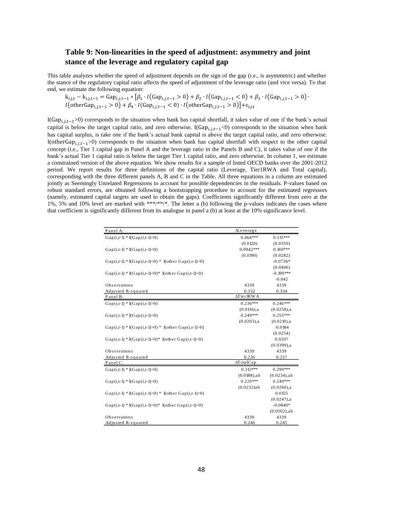
48

Table 9: Non-linearities in the speed of adjustment: asymmetry and joint

stance of the leverage and regulatory capital gap

This table analyzes whether the speed of adjustment depends on the sign of the gap (i.e., is asymmetric) and whether

the stance of the regulatory capital ratio affects the speed of adjustment of the leverage ratio (and vice versa). To that

end, we estimate the following equation:

k𝑖,j,𝑡 − k𝑖,j,𝑡−1 = Gap𝑖,𝑗,𝑡−1 ∗ [𝛽1 ∙ 𝐼(Gap𝑖,𝑗,𝑡−1 > 0) + 𝛽2 ∙ 𝐼(Gap𝑖,𝑗,𝑡−1 < 0) + 𝛽3 ∙ 𝐼(Gap𝑖,𝑗,𝑡−1 > 0) ∙

𝐼(otherGap𝑖,𝑗,𝑡−1 > 0) + 𝛽4 ∙ 𝐼(Gap𝑖,𝑗,𝑡−1 < 0) ∙ 𝐼(otherGap𝑖,𝑗,𝑡−1 > 0)]+εi,j,t

I(Gap𝑖,𝑗,𝑡−1>0) corresponds to the situation when bank has capital shortfall, it takes value of one if the bank’s actual

capital is below the target capital ratio, and zero otherwise. I(Gap𝑖,𝑗,𝑡−1<0) corresponds to the situation when bank

has capital surplus, is take one if the bank’s actual bank capital is above the target capital ratio, and zero otherwise.

I(otherGap𝑖,𝑗,𝑡−1>0) corresponds to the situation when bank has capital shortfall with respect to the other capital

concept (i.e., Tier 1 capital gap in Panel A and the leverage ratio in the Panels B and C), it takes value of one if the

bank’s actual Tier 1 capital ratio is below the target Tier 1 capital ratio, and zero otherwise. In column 1, we estimate

a constrained version of the above equation. We show results for a sample of listed OECD banks over the 2001-2012

period. We report results for three definitions of the capital ratio (Leverage, Tier1RWA and Total capital),

corresponding with the three different panels A, B and C in the Table. All three equations in a column are estimated

jointly as Seemingly Unrelated Regressions to account for possible dependencies in the residuals. P-values based on

robust standard errors, are obtained following a bootstrapping procedure to account for the estimated regressors

(namely, estimated capital targets are used to obtain the gaps). Coefficients significantly different from zero at the

1%, 5% and 10% level are marked with ***/**/*. The letter a (b) following the p-values indicates the cases where

that coefficient is significantly different from its analogue in panel a (b) at least at the 10% significance level.

P an el A: ∆Leverag e

Gap (i,t-1) * I(Gap (i,t-1)>0) 0.464*** 0.515***

(0.0120) (0.0359)

Gap (i,t-1) * I(Gap (i,t-1)<0) 0.0942*** 0.169***

(0.0190) (0.0282)

Gap (i,t-1) * I(Gap (i,t-1)>0) * I(oth er Gap (i,t-1)>0) -0.0736*

(0.0406)

Gap (i,t-1) * I(Gap (i,t-1)<0)* I(oth er Gap (i,t-1)>0) -0.190***

-0.042

Ob s ervation s 4339 4339

Ad ju s ted R-s q u ared 0.332 0.334

P an el B: ∆Tier1RW A

Gap (i,t-1) * I(Gap (i,t-1)>0) 0.236*** 0.246***

(0.0136),a (0.0258),a

Gap (i,t-1) * I(Gap (i,t-1)<0) 0.249*** 0.255***

(0.0203),a (0.0210),a

Gap (i,t-1) * I(Gap (i,t-1)>0) * I(oth er Gap (i,t-1)>0) -0.0184

(0.0254)

Gap (i,t-1) * I(Gap (i,t-1)<0)* I(oth er Gap (i,t-1)>0) 0.0207

(0.0399),a

Ob s ervation s 4339 4339

Ad ju s ted R-s q u ared 0.236 0.237

P an el C: ∆TotalCap

Gap (i,t-1) * I(Gap (i,t-1)>0) 0.313*** 0.299***

(0.0188),ab (0.0234),ab

Gap (i,t-1) * I(Gap (i,t-1)<0) 0.220*** 0.249***

(0.0232)ab (0.0260),a

Gap (i,t-1) * I(Gap (i,t-1)>0) * I(oth er Gap (i,t-1)>0) 0.0155

(0.0247),a

Gap (i,t-1) * I(Gap (i,t-1)<0)* I(oth er Gap (i,t-1)>0) -0.0840*

(0.0502),ab

Ob s ervation s 4339 4339

Ad ju s ted R-s q u ared 0.246 0.245

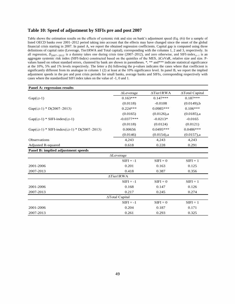
49

Table 10: Speed of adjustment by SIFIs pre and post 2007

Table shows the estimation results on the effects of systemic risk and size on bank’s adjustment speed (Eq. (6)) for a sample of

listed OECD banks over 2001–2012 period taking into account that the effects may have changed since the onset of the global

financial crisis starting in 2007. In panel A, we report the obtained regression coefficients. Capital gap is computed using three

definitions of capital ratio (Leverage, Tier1RWA and Total capital), corresponding with the columns 1, 2 and 3, respectively. In

all regression, 𝐷2007−2012 is a dummy takes one during crisis time (2007–2012), and zero otherwise, and SIFI-indexi,t−1 is an

aggregate systemic risk index (SIFI-Index) constructed based on the quintiles of the MES, ∆CoVaR, relative size and size. P-

values based on robust standard errors, clustered by bank are shown in parentheses. *, ** and*** indicate statistical significance

at the 10%, 5% and 1% levels respectively. The letter a (b) following the p-values indicates the cases where that coefficient is

significantly different from its analogue in column 1 (2) at least at the 10% significance level. In panel B, we report the implied

adjustment speeds in the pre and post crisis periods for small banks, average banks and SIFIs, corresponding respectively with

cases where the standardized SIFI index takes on the value of -1, 0 and 1.

Panel A: regression results

∆Leverage ∆Tier1RWA ∆Total Capital

Gap(i,t-1) 0.163*** 0.147*** 0.187***

(0.0118) -0.0108 (0.0149),b

Gap(i,t-1) * D(2007–2013) 0.224*** 0.0985*** 0.106***

(0.0165) (0.0126),a (0.0185),a

Gap(i,t-1) * SIFI-index(i,t-1) -0.0377*** -0.0213* -0.0165

(0.0118) (0.0124) (0.0121)

Gap(i,t-1) * SIFI-index(i,t-1) * D(2007–2013) 0.00656 0.0495*** 0.0486***

(0.0146) (0.0154),a (0.0157),a

Observations 4,243 4,243 4,243

Adjusted R-squared 0.618 0.228 0.291

Panel B: implied adjustment speeds

SIFI = -1 SIFI = 0 SIFI = 1

2001-2006 0.201 0.163 0.125

2007-2013 0.418 0.387 0.356

SIFI = -1 SIFI = 0 SIFI = 1

2001-2006 0.168 0.147 0.126

2007-2013 0.217 0.245 0.274

SIFI = -1 SIFI = 0 SIFI = 1

2001-2006 0.204 0.187 0.171

2007-2013 0.261 0.293 0.325

∆Leverage

∆Tier1RWA

∆Total Capital

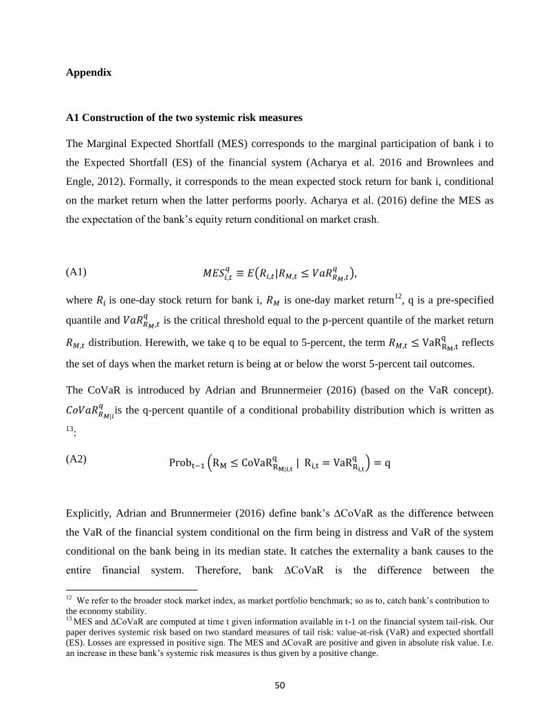
50

Appendix

A1 Construction of the two systemic risk measures

The Marginal Expected Shortfall (MES) corresponds to the marginal participation of bank i to

the Expected Shortfall (ES) of the financial system (Acharya et al. 2016 and Brownlees and

Engle, 2012). Formally, it corresponds to the mean expected stock return for bank i, conditional

on the market return when the latter performs poorly. Acharya et al. (2016) define the MES as

the expectation of the bank’s equity return conditional on market crash.

(A1) 𝑀𝐸𝑆𝑖,𝑡𝑞 ≡ 𝐸(𝑅𝑖,𝑡|𝑅𝑀,𝑡 ≤ 𝑉𝑎𝑅𝑅𝑀,𝑡

𝑞 ),

where 𝑅𝑖 is one-day stock return for bank i, 𝑅𝑀 is one-day market return12

, q is a pre-specified

quantile and 𝑉𝑎𝑅𝑅𝑀,𝑡𝑞

is the critical threshold equal to the p-percent quantile of the market return

𝑅𝑀,𝑡 distribution. Herewith, we take q to be equal to 5-percent, the term 𝑅𝑀,𝑡 ≤ VaRRM,tq

reflects

the set of days when the market return is being at or below the worst 5-percent tail outcomes.

The CoVaR is introduced by Adrian and Brunnermeier (2016) (based on the VaR concept).

𝐶𝑜𝑉𝑎𝑅𝑅𝑀|𝑖𝑞

is the q-percent quantile of a conditional probability distribution which is written as

13:

(A2) Probt−1 (RM ≤ CoVaRRM|i,tq

| Ri,t = VaRRi,tq) = q

Explicitly, Adrian and Brunnermeier (2016) define bank’s ∆CoVaR as the difference between

the VaR of the financial system conditional on the firm being in distress and VaR of the system

conditional on the bank being in its median state. It catches the externality a bank causes to the

entire financial system. Therefore, bank ∆CoVaR is the difference between the

12

We refer to the broader stock market index, as market portfolio benchmark; so as to, catch bank’s contribution to

the economy stability. 13

MES and ∆CoVaR are computed at time t given information available in t-1 on the financial system tail-risk. Our

paper derives systemic risk based on two standard measures of tail risk: value-at-risk (VaR) and expected shortfall

(ES). Losses are expressed in positive sign. The MES and ∆CovaR are positive and given in absolute risk value. I.e.

an increase in these bank’s systemic risk measures is thus given by a positive change.

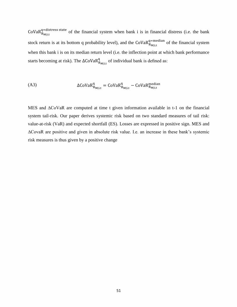
51

CoVaRRM|i,tq=distress state

of the financial system when bank i is in financial distress (i.e. the bank

stock return is at its bottom q probability level), and the CoVaRRM|i,tq=median

of the financial system

when this bank i is on its median return level (i.e. the inflection point at which bank performance

starts becoming at risk). The ∆CoVaRRM|i,tq

of individual bank is defined as:

(A3) ∆CoVaRRM|i,tq

= CoVaRRM|i,tq

− CoVaRRM|i,tmedian

MES and ∆CoVaR are computed at time t given information available in t-1 on the financial

system tail-risk. Our paper derives systemic risk based on two standard measures of tail risk:

value-at-risk (VaR) and expected shortfall (ES). Losses are expressed in positive sign. MES and

∆CovaR are positive and given in absolute risk value. I.e. an increase in these bank’s systemic

risk measures is thus given by a positive change

NBB WORKING PAPER No. 369 – MARCH 2019 53

NATIONAL BANK OF BELGIUM - WORKING PAPERS SERIES

The Working Papers are available on the website of the Bank: http://www.nbb.be.

317. “An estimated two-country EA-US model with limited exchange rate pass-through”, by G. de Walque,Ph. Jeanfils, T. Lejeune, Y. Rychalovska and R. Wouters, Research series, March 2017.

318. Using bank loans as collateral in Europe: The role of liquidity and funding purposes”, by F. Koulischer andP. Van Roy, Research series, April 2017.

319. “The impact of service and goods offshoring on employment: Firm-level evidence”, by C. Ornaghi,I. Van Beveren and S. Vanormelingen, Research series, May 2017.

320. “On the estimation of panel fiscal reaction functions: Heterogeneity or fiscal fatigue?”, by G. Everaert andS. Jansen, Research series, June 2017.

321. “Economic importance of the Belgian ports: Flemish maritime ports, Liège port complex and the port ofBrussels - Report 2015”, by C. Mathys, Document series, June 2017.

322. “Foreign banks as shock absorbers in the financial crisis?”, by G. Barboni, Research series, June 2017.323. “The IMF and precautionary lending: An empirical evaluation of the selectivity and effectiveness of the

flexible credit line”, by D. Essers and S. Ide, Research series, June 2017.324. “Economic importance of air transport and airport activities in Belgium – Report 2015”, by S. Vennix,

Document series, July 2017.325. “Economic importance of the logistics sector in Belgium”, by H. De Doncker, Document series, July 2017.326. “Identifying the provisioning policies of Belgian banks”, by E. Arbak, Research series, July 2017.327. “The impact of the mortgage interest and capital deduction scheme on the Belgian mortgage market”, by

A. Hoebeeck and K. Inghelbrecht, Research series, September 2017.

328. “Firm heterogeneity and aggregate business services exports: Micro evidence from Belgium, France,Germany and Spain”, by A. Ariu, E. Biewen, S. Blank, G. Gaulier, M.J. González, Ph. Meinen, D. Mirza,C. Martín and P. Tello, Research series, September 2017.

329. “The interconnections between services and goods trade at the firm-level”, by A. Ariu, H. Breinlichz,G. Corcosx, G. Mion, Research series, October 2017.

330. “Why do manufacturing firms produce services? Evidence for the servitization paradox in Belgium”, byP. Blanchard, C. Fuss and C. Mathieu, Research series, November 2017.

331. “Nowcasting real economic activity in the euro area: Assessing the impact of qualitative surveys”, byR. Basselier, D. de Antonio Liedo and G. Langenus, Research series, December 2017.

332. “Pockets of risk in the Belgian mortgage market: Evidence from the Household Finance and ConsumptionSurvey (HFCS)”, by Ph. Du Caju, Research series, December 2017.

333. “The employment consequences of SMEs’ credit constraints in the wake of the great recession” byD. Cornille, F. Rycx and I. Tojerow, Research series, December 2017.

334. “Exchange rate movements, firm-level exports and heterogeneity”, by A. Berthou and E. Dhyne, Researchseries, January 2018.

335 “Nonparametric identification of unobserved technological heterogeneity in production”, by L. Cherchye,T. Demuynck, B. De Rock and M. Verschelde, Research series, February 2018.

336 “Compositional changes in aggregate productivity in an era of globalisation and financial crisis”, by C. Fussand A. Theodorakopoulos, Research series, February 2018.

337. “Decomposing firm-product appeal: How important is consumer taste?”, by B. Y. Aw, Y. Lee andH. Vandenbussche, Research series, March 2018.

338 “Sensitivity of credit risk stress test results: Modelling issues with an application to Belgium”, byP. Van Roy, S. Ferrari and C. Vespro, Research series, March 2018.

339. “Paul van Zeeland and the first decade of the US Federal Reserve System: The analysis from a Europeancentral banker who was a student of Kemmerer”, by I. Maes and R. Gomez Betancourt, Research series,March 2018.

340. “One way to the top: How services boost the demand for goods”, by A. Ariu, F. Mayneris and M. Parenti,Research series, March 2018.

341 “Alexandre Lamfalussy and the monetary policy debates among central bankers during the Great Inflation”,by I. Maes and P. Clement, Research series, April 2018.

342. “The economic importance of the Belgian ports: Flemish maritime ports, Liège port complex and the portof Brussels – Report 2016”, by F. Coppens, C. Mathys, J.-P. Merckx, P. Ringoot and M. Van Kerckhoven,Document series, April 2018.

343. “The unemployment impact of product and labour market regulation: Evidence from European countries”,by C. Piton, Research series, June 2018.

344. “Trade and domestic production networks”, by F. Tintelnot, A. Ken Kikkawa, M. Mogstad, E. Dhyne,Research series, September 2018.

54 NBB WORKING PAPER No. 369 – MARCH 2019

345. “Review essay: Central banking through the centuries”, by I. Maes, Research series, October 2018.346. “IT and productivity: A firm level analysis”, by E. Dhyne, J. Konings, J. Van den Bosch, S. Vanormelingen,

Research series, October 2018.347. “Identifying credit supply shocks with bank-firm data: methods and applications”, by H. Degryse,

O. De Jonghe, S. Jakovljević, Klaas Mulier, Glenn Schepens, Research series, October 2018.348. “Can inflation expectations in business or consumer surveys improve inflation forecasts?”, by R. Basselier,

D. de Antonio Liedo, J. Jonckheere and G. Langenus, Research series, October 2018.349. “Quantile-based inflation risk models”, by E. Ghysels, L. Iania and J. Striaukas, Research series,

October 2018.350. “International food commodity prices and missing (dis)inflation in the euro area”, by G. Peersman,

Research series, October 2018.351. “Pipeline pressures and sectoral inflation dynamics”, by F. Smets, J. Tielens and J. Van Hove, Research

series, October 2018.352. “Price updating in production networks”, by C. Duprez and G. Magerman, Research series, October 2018.353. “Dominant currencies. How firms choose currency invoicing and why it matters”, by M. Amiti, O. Itskhoki

and J. Konings, Research series, October 2018.354. “Endogenous forward guidance”, by B. Chafwehé, R. Oikonomou, R. Priftis and L. Vogel, Research series,

October 2018.355. “Is euro area Iowflation here to stay? Insights from a time-varying parameter model with survey data”, by

A. Stevens and J. Wauters, Research series, October 2018.356. “A price index with variable mark-ups and changing variety”, by T. Demuynck and M. Parenti, Research

series, October 2018.357. “Markup and price dynamics: Linking micro to macro”, by J. De Loecker, C. Fuss and J. Van Biesebroeck,

Research series, October 2018.358. “Productivity, wages and profits: Does firms’ position in the value chain matter?”, by B. Mahy, F. Rycx,

G. Vermeylen and M. Volral, Research series, October 2018.359. “Upstreamness, social upgrading and gender: Equal benefits for all?”, by N. Gagliardi, B. Mahy and

F. Rycx, Research series, December 2018.360. “A macro-financial analysis of the corporate bond market”, by H. Dewachter, L. Iania, W. Lemke and

M. Lyrio, Research series, December 2018.361. “Some borrowers are more equal than others: Bank funding shocks and credit reallocation”, by

O. De Jonghe, H. Dewachter, K. Mulier, S. Ongena and G. Schepens, Research series, December 2018.362. “The origins of firm heterogeneity: A production network approach”, by A. B. Bernard, E. Dhyne,

G. Magerman, K. Manova and A. Moxnes, Research series, January 2019.363. “Imperfect competition in firm-to-firm trade”, by A. Ken Kikkawa, G. Magerman and E. Dhyne, Research

series, January 2019.364. “Forward guidance with preferences over safe assets”, by A. Rannenberg, Research series, January 2019.365. “The distinct effects of information technologies and communication technologies on the age-skill

composition of labour demand”, by S. Blanas, Research series, January 2019.366. “A survey of the long-term impact of Brexit on the UK and the EU27 economies”, by P. Bisciari, Document

series, January 2019.367. “A macroeconnomic model with heterogeneous and financially-constrained intermediaries”, by Th. Lejeune

and R. Wouters, Research series, February 2019.368. “The economic importance of the Belgian ports: Flemish maritime ports, Liège port complex and the port

of Brussels – Report 2017”, by E. Gueli, P. Ringoot and M. Van Kerckhoven, Document series, March2019.

369. “Does banks’ systemic importance affect their capital structure and balance sheet adjustment processes?”,by Y. Bakkar, O. De Jonghe and A. Tarazi, Research series, March 2019.

© Illustrations : National Bank of Belgium

Layout : Analysis and Research Group Cover : NBB AG – Prepress & Image

Published in March 2019

Editor

Pierre WunschGovernor of the National Bank of Belgium

National Bank of Belgium Limited liability company RLP Brussels – Company’s number : 0203.201.340 Registered office : boulevard de Berlaimont 14 – BE -1000 Brussels www.nbb.be