Documentation of the TIMES-MACRO model - IEA-ETSAP · Energy Technology Systems Analysis Programme Documentation of the TIMES-MACRO model DRAFT Version Uwe Remme, Markus Blesl

Energy Technology Systems Analysis Programme

http://www.etsap.org

Documentation of the TIMES-MACRO model

DRAFT Version

Uwe Remme, Markus Blesl

February 1, 2006

Contents

1. Introduction ....................................................................................................................... 1

2. Concept of the TIMES-MACRO model............................................................................ 1 2.1. Basic formulation of the MACRO model .......................................................................... 3 2.2. Linkage of the TIMES and MACRO model...................................................................... 7 2.3. Calibration of a TIMES-MACRO model .......................................................................... 8

2.3.1. Initial values .................................................................................................................................... 8 2.3.2. Parameters of the production function ............................................................................................ 8 2.3.3. Calibration routine .......................................................................................................................... 9

3. Reference Guide for TIMES-MACRO ........................................................................... 10 3.1. Parameters of the TIMES MACRO model ..................................................................... 10

3.1.1. User-input parameters ................................................................................................................... 11 3.1.2. Internal parameters........................................................................................................................ 16

3.2. Variables of the TIMES MACRO model......................................................................... 22 3.3. Equations of the MACRO model...................................................................................... 23

3.3.1. Objective function......................................................................................................................... 24 3.3.2. Capital dynamics equation ............................................................................................................ 27 3.3.3. Terminal condition for investment in last period .......................................................................... 28 3.3.4. Demand decoupling equation........................................................................................................ 29 3.3.5. Bound on the sum of investment and energy ................................................................................ 30 3.3.6. Annual cost of energy ................................................................................................................... 31 3.3.7. Variable definition for market penetration cost penalty function.................................................. 33 3.3.8. Market penetration cost penalty function, quadratic approximation ............................................. 33

3.4. Precalculations ................................................................................................................... 34 3.4.1. Utility discount factor.................................................................................................................... 34 3.4.2. Initial values .................................................................................................................................. 35 3.4.3. Coefficients of the production function......................................................................................... 35 3.4.4. Further precalculations.................................................................................................................. 37

3.5. Variable bounds and starting values................................................................................ 38 3.6. TIMES-MACRO specific reporting parameters............................................................. 40

4. Calibrating a TIMES-MACRO model............................................................................ 42 4.1. DDFNEW0.......................................................................................................................... 43 4.2. DDFNEW............................................................................................................................ 45 4.3. Running the calibration routine ....................................................................................... 46

5. Running a TIMES-MACRO model ................................................................................ 50

6. Solution issues ................................................................................................................. 53 6.1. Reduction algorithm .......................................................................................................... 53 6.2. Solver................................................................................................................................... 53 6.3. Starting values.................................................................................................................... 53

Literature ................................................................................................................................. 54

List of Tables Table 1: TIMES-MACRO user-input parameters .............................................................. 11 Table 2: TIMES-MACRO internal parameters .................................................................. 16 Table 3: TIMES-MACRO variables .................................................................................. 22 Table 4: Equations of the MACRO model ......................................................................... 23

List of Figures Figure 1: Concept of the linkage in the TIMES-MACRO model.......................................... 2 Figure 2: Overview of the calibration procedure of a TIMES-MACRO model.................. 43 Figure 3: Example of a batch file for calibrating a TIMES-MACRO ................................. 47 Figure 4: Content of the file macro.dd ................................................................................ 48 Figure 5: Content of the file gr.dd ....................................................................................... 48 Figure 6: File structure of the calibration process ............................................................... 49 Figure 7: Content of the file ddf.dd...................................................................................... 52

1

1. Introduction This document describes the linkage of the energy systems model TIMES with the one-sectoral general equilibrium model MACRO leading to the merged model TIMES-MACRO. The approach of linking TIMES and MACRO is very similar to the linkage of the MARKAL model, the ancestor of TIMES, with the MACRO model (see /Manne and Wene 1992/, /Kypreos 1997/, /Loulou, et. al. 2004/). A great part of the MARKAL code related to the MACRO model has been used as basis for the TIMES formulation. In the following chapter a simplified formulation of the MACRO model and the general concept of linking TIMES with MACRO are presented. Chapter 3 serves as reference guide for TIMES-MACRO. It gives an overview of the user input parameters for building a as well as internal parameters of the GAMS implementation. The equations and associated variables of the MACRO model are also presented there. Details on the derivation of some coefficients of the MACRO equations, information on bounds and starting values for the MACRO variables as well as an overview of the reporting parameters are also given in Chapter 3. The routines for calibrating the TIMES-MACRO model are described in Chapter 4 followed by a short description of running the TIMES-MACRO model (Chapter 5) and a discussion on some solution issues (Chapter 6).

2. Concept of the TIMES-MACRO model The TIMES-MACRO model is a result of linking the bottom-up energy systems model TIMES with the top-down model MACRO. Bottom-up models as TIMES describe the energy sector in technology-rich way, but ignore the interdependencies of the energy sector with the remaining economy. On the other hand top-down models as MACRO, which depict the economic relationships of the entire economy, enable one to study the interconnections between economic development and energy demand. Since this is done on a more aggregate level, detailed technology related information cannot be derived from top-down models. To circumvent the shortcomings present in the two modeling approaches, several developments have been undertaken to extend the methodology in the corresponding other direction, i.e., technological detail has been added to top-down models (see e.g. /Böhringer 1998/, /Böhringer and Rutherford 2005/) and information on the interconnection of the energy sector with the remaining economy has been added to bottom-up models (see e.g. /Manne and Wene 1992/). The latter approach is the basis of the TIMES-MACRO model presented here. The concept of the MACRO model and its linkage with the TIMES model will be presented in this section. For detailed information on the TIMES model the reader is referred to the model documentation (/Loulou, et. al. 2005/).

2

The MACRO model, which can be characterized as a single-sector, optimal growth dynamic inter-temporal general equilibrium model, maximizes the national (regional) utility. The utility is a logarithmic function of the consumption of a single generic consumer. The industry sectors outside of the energy sector are presented by the production function of a single representative industry sector. Inputs for the production are labor, capital and energy. The energy demand is covered by the energy sector, which is represented by the TIMES model. Part of the annual production is used to cover the costs for energy demand. The other part can be used for investments in the capital stock or for consumption by the households. Thus, the linkage between the MACRO model and the TIMES model is established in two directions: the TIMES model provides the costs of the energy demand to the MACRO model, while in the other direction the MACRO model determines the energy demand being input factor for the TIMES model. The linkage of the two models is shown in Figure 1.

TIMES MACRO

Labor

Consumption

Investment

Capital

Energy costs

Energy demand

Figure 1: Concept of the linkage for a single-region TIMES-MACRO model

Government is not represented in the TIMES-MACRO model. The approach implemented so far works only for a single-regional model. The equilibrium of the single-regional model is characterized by a maximum of the region’s utility or welfare and can be computed by solving a non-linear programming (NLP) problem. In a multi-regional context, each region seeks to maximize its utility. The regions are linked through trade in goods. The calculation of the equilibrium for a multi-regional model is much more complex. Approaches to find solutions for multi-regional problems are presented for MARKAL-MACRO in /Büeler 1997/. An alternative solution route is to separate MACRO from the energy part and to solve the overall problem in an iterative way.

3

2.1. Basic formulation of the MACRO model To describe the general ideal of the MACRO model its basic mathematical formulation is given by the equations (1) – (6)1:

)ln(1

)ln(2

2111

11

1

Tdd

T

dd

TTt

T

tt C

dfactcurr

dfactcurrdfactCdfactMax

TT

TT

⋅−

⋅+⋅ +

+

−−−

=−

−

∑ (1)

tttt ECINVCY ++= (2)

ρρρ ρ

1

,)1( ⎟

⎠

⎞⎜⎝

⎛⋅+⋅⋅= ∑−⋅

dmdmtdm

kpvst

kpvsrt DEM_MblKaklY (3)

( ) 211

1

1 and1++

+ +⋅==tt dd

ttt growvlll (4)

( )1t1ttttt1t INVdINVtsrvdKtsrvK +++ ⋅+⋅⋅+⋅=21 (5)

( ) TTT INVdeprgrowvK ≤+⋅ (6)

with the model variables

tC : annual consumption in period t,

t,dmDEM_M : annual energy demand in MACRO for commodity dm in period t,

tY : annual production in period t,

tINV : annual investments in period t,

tEC : annual energy costs in period t,

tK : total capital in period t

and the exogenously determined parameters akl : production function constant,

dmb : demand coefficient,

td : duration of period t in years,

depr : depreciation rate,

1 The concrete implementation in the TIMES-MACRO model differs in some points, e.g. the consumption variable in the utility function is substituted by equations (2) and (3). The exact formulation as implemented in TIMES is given further below in Chapter 3.

4

tdfact : utility discount factor,

tdfactcurr : annual discount rate,

tgrowv : growth rate in period t,

kpvs capital value share,

tl : annual labor index in period t,

ρ : substitution constant,

T : period index of the last period,

ttsrv : capital survival factor between two periods.

The objective function (1) of the MACRO model is the maximization of the discounted utility. The utility is defined through the consumption tC of the households. A logarithmic

utility function has been chosen, instead of a linear one, to avoid “bang-bang” solutions related to linear functions. Due to the concave nature of the utility function the additional utility of consumption is decreasing with increasing consumption (diminishing marginal utility). To measure the utility, consumption and not GDP (gross domestic product) has been selected, since GDP contains in addition to consumption investments. The discount factor of the last period has a larger impact. It is assumed that the utility of the last period will be valid for the infinite time horizon after the last model period leading to a larger value of the discount factor. The derivation of the discount factors is discussed in Section 3.4.1. The production function (3) is a nested, constant elasticity of substitution (CES) function with the input factors capital, labor and energy. The production input factors labor tl and capital

tK form an aggregate KLA , in which both can be substituted by each other represented by a

Cobb-Douglas function. Then, the aggregate of the energy services and the aggregate of capital and labor can substitute each other. The elasticity of substitution between the aggregate of capital and labor on the one side and energy on the other side is the ratio between the relative change in the quotient of two production factors and the relative change in their prices. For the production factors energy E and the aggregate of capital and labor KLA the elasticity of substitution has the general form:

( )( )EKL

KL

E

KL

E

KL

KLKL

PPEA

PP

PP

EA

EA

lnln)

∂∂

=

⎟⎟⎠

⎞⎜⎜⎝

⎛∂

⎟⎠⎞

⎜⎝⎛∂

=σ (7)

with

5

σ : elasticity of substitution,

KLA : aggregate of capital and labor,

E : energy,

KLP : price for the production factor aggregate of capital and labor,

EP : price for the production factor energy.

For Western European economies the elasticity of substitution has been estimated to be in the range of 0.2 to 0.5 /Läge 2001/. The lower the value of the elasticity of substitution the closer is the linkage between economic growth and increase in energy demand. For homogenous production functions with constant scale of returns2 the substitution constant ρ in Eqn. (3) is

directly linked with the user-given elasticity of substitution σ by the expression σρ 11−= .

The capital value share kpvs describes the share of capital in the sum of all production factors

and has to be specified by the user. For OECD economies, rtm_kpvs typically lies in the

range from 0.2 to 0.3. The parameter akl is the level constant of the production function. The parameters akl and dmb of the production are determined based on the results from a TIMES

model run without the MACRO module (see Section 3.4.3). Equation (2) describes how the annual production tY spent. The consumers, who want to

maximize their utility over the model horizon, can decide whether they want to spend the production for consumption in the current period or whether they want to use use tY for

investments, which can be used for future consumption. In addition, the production has to cover the costs for the production of energy tEC .

The production factor labor (Eqn. (4)) is modeled has efficiency indicator having a value of 1 for the first period. It is not an endogenous model variable in MACRO, but specified exogenously by the labor growth rate tgrowv . The increase in the production factor labor can

be caused by an increase in population but also by efficiency improvements in the productivity. The efficiency improvements can be interpreted as a form of technical progress. This type of efficiency improvement, which is only subject to the production factor labor, is called Harrod-neutral or labor augmenting technical progress. It should be noted that the

2 A production function is called homogenous of degree r, if multiplying all production factors by a constant scalar leads λ to an increase of the function by rλ :

( )( )LKfY

LKfYr λλλ ,

,=

=.

If r = 1, the production function is called linearly homogenous and leads to constant returns of scale.

6

exogenously specified labor growth rate tgrowv is only a potential growth rate, the real GDP

growth rate is calculated endogenously by the model. The purpose of the calibration routine described in Section 4 is to adjust the labor growth rates tgrowv in such a way that a user-

specified GDP growth rate (input parameter tm_gr ) is matched.

The capital dynamics equations (5) describes the capital stock in the current period 1tK +

based on the capital stock in the previous period and on investments made in the current and the previous period. Depreciation leads to a reduction of the capital. This effect is taken into account by the capital survival factor ttsrv . It describes the share of the capital or investment

in period t that still exists in period t+1. It is derived from the depreciation rate depr using

the following expression:

( )( )

21

1tt dd

t deprtsrv++

−= (8)

Expression (8) calculates the capital survival factor for a period of years beginning with the end of the middle year tm and ending with the end of the year 1+tm . The duration between

these two middle years equals the duration 2

1 tt dd ++ . Then, a mean investment in period t is

calculated by weighting the investments in t and t+1 with the respective period duration: ( )1t1ttt INVdINVtsrvd ++ ⋅+⋅⋅21 .

For the first period it is assumed that the capital stock grows with the labor growth rate of the first period 0growv . Thus, the investment has to cover this growth rate plus the depreciation

of capital. Since the initial capital stock is given and the depreciation and growth rates are exogenously, the investment in the first period can be calculated beforehand:

( )0growvdeprKINV 00 +⋅= (9)

Since the model horizon is finite, one has to ensure that the capital stock is not fully exhausted which would maximize the utility in the model horizon. Therefore a terminal condition (6) is added, which guarantees, that also after the end of the model horizon a capital stock for the following generations exists. It is assumed that the capital stock grows with the labor growth rate Tgrowv . This is coherent with the last term of the utility function.

7

2.2. Linkage of the TIMES and MACRO model As shown in Figure 1 the TIMES model and the MACRO model are connected by two flows of information: the annual energy costs calculated by the TIMES model are passed to the MACRO model, whereas in the opposite direction the demand for energy determined by the MACRO model is given as input information to the TIMES model. Eqn. (10) links the MACRO energy demand t,dmDEM_M with the energy demand t,dmDEM_T in the TIMES

model.

t,dmdmtt,dm DEM_MaeeifacDEM_T ⋅= , (10)

The energy demand effective in the TIMES model can be lower than the energy requirement of the MACRO model due to demand reductions, which are caused by autonomous energy efficiency improvements and which are not already captured in the energy sector of the TIMES model. These efficiency improvements are captured by the autonomous energy efficiency improvement factor dmtaeeifac , . It is determined in a calibration procedure

described in Chapter 4. The costs tEC for covering the energy demand determined by the MACRO model are

calculated by the TIMES model as costs tCOST_T :

tp

2t,p

pt

ptt ECXCAP

capfyexpfcstinv

qfacCOST_T =⋅⋅

+ ∑ ,

21 (11)

with

tCOST_T : annual undiscounted energy system costs of the TIMES model,

t,pXCAP : Penalized capacity expansion for technology p in period t exceeding a

predefined tolerable expansion,

tEC : costs for the production factor energy in the MACRO model,

qfac : trigger to activate penalty term (0 for turning-off penalty, 1 for using penalty

term),

ptcstinv , : specific annualized investment costs of technology p in period t,

pcapfy : maximum level of capacity for technology p,

texpf : tolerable expansion between two periods.

8

To slow down the penetration a quadratic penalty term has been added on the left hand side of Eqn. (11). The variable ptXCAP, is the amount of capacity exceeding a predefined expansion

level expressed by the expansion factor texpf and is determined by the following equation:

( ) ptpttpt XCAPCAPexpfCAP ,1,,1 1 ++ +⋅+≤ (12)

with

t,pCAP : total installed capacity of technology p in period t.

As long as the total installed capacity in period t+1 is below ( ) ptt CAPexpf ,1 ⋅+ no penalty

costs are applied. For the capacity amount ptXCAP ,1+ exceeding this tolerated capacity level

penalty costs are added to the regular costs of the TIMES model in Eqn. (11). Since the quadratic term in Eqn. (11) introduces a nonlinear term for each technology and period, it may cause solution problems for large models and is hence replaced in the current implementation of TIMES, as in MARKAL, by a linear approximation (see Section 3.3.6 for details).

2.3. Calibration of a TIMES-MACRO model 2.3.1. Initial values Based on macroeconomic statistics the MACRO variables for the first period can be estimated. When the initial GDP, the capital-to-GDP value kgdp , the depreciation rate depr

and the potential growth rate growv are given, the initial capital stock 0K , the initial

investment 0I , the initial consumption 0C , the initial production 0Y can be calculated. The

energy demand vector of the MACRO model is set equal to the demand vector of the stand-alone TIMES model for the first period. The calculation of these initial values is described in more detail in Section 3.4.2. 2.3.2. Parameters of the production function For the production function (Eqn. (3)) the substitution constant ρ , the capital value share

kpvs , the level constant akl and the demand coefficients dmb have to be provided.

The substitution constant ρ is based on the elasticity of substitution σ by the expression

σρ 11−= . The elasticity of substitution for the production factor energy is difficult to

9

obtain. For Western European economies the elasticity of substitution has been estimated to be in the range of 0.2 to 0.5 /Läge 2001/. A high value indicates a higher substitution reaction to price changes, while the opposite is true for low values. Hence, /Loulou, et. al. 2004/ argue that for energy system models having a detailed representation of the end-use sectors with energy substitution and saving options, the elasticity of substitution should be in the lower range, while for models with a limited representation of the end-use sectors the flexibility to substitute energy by the aggregate and labor should be higher, which is expressed by a larger value for the elasticity of substitution. With the partial derivative of the production function with respect to the energy demands dm the demand coefficients dmb can be estimated by solving the partial derivates for the dmb

coefficients:

dm0,dm

0dm

tt,dm

t bDEM_M

YprefVAR_D

VAR_Yρ−

=⎟⎟⎠

⎞⎜⎜⎝

⎛==

∂∂

1

,0

0

(13)

The prices dmpref ,0 are obtained from a stand-alone TIMES model run as the undiscounted

shadow prices of the demand commodities in the first period. Since the first period(s) are usually used for calibrating the energy system model, the shadow prices in these periods are usually degenerated due to an overdetermined equation system. Therefore, it is advised to take the shadow prices of a following undisturbed period. After the calculation of dmb , the level

constant akl can be computed from the production function for the initial period. 2.3.3. Calibration routine The purpose of the calibration routine is twofold. First, it should determine the autonomous energy efficiency improvement factor dmtaeeifac , of Eqn. (10) in such a way that the values of

the TIMES demand variables r,t,dmDEM_T match the exogenously specified demand

parameters t,dmcom_proj of the stand-alone TIMES model. As a result of this calibration step

the results in the energy system part of the linked TIMES-MACRO model are identical to the ones when running the stand-alone TIMES model. Secondly, the calibration routine should calculate the labor growth rates tgrowv such that user-specified GDP growth rates tm_gr are

matched.

10

3. Reference Guide for TIMES-MACRO This chapter serves as reference guide for TIMES-MACRO. It gives an overview of the user input parameters (Section 3.1.1) for building a as well as internal parameters of the GAMS implementation (Section 3.1.2). Then the equations and associated variables (Section 3.2, 3.3) of the MACRO model are presented. Details on the derivation of some coefficients of the MACRO equations (Section 3.4), information on bounds and starting values for the MACRO variables (Section 3.5) as well as an overview of the reporting parameters (Section 3.6) are also given. 3.1. Parameters of the TIMES MACRO model In this chapter the parameters used in the MACRO model are described. One can distinguish between user-input parameters, which are provided by the user, and internal parameters, which are derived internally based on the user-input parameters within the GAMS code of the MACRO module. The utility discount factors in the objective function are an example for internal parameters. To distinguish the parameters relevant for the MACRO model from the parameters of the TIMES model, the MACRO related parameters have the suffix “ _tm ”. The MACRO

parameters also have a regional index, although the current implementation does not work for multi-regional models3. The regional index was however added for programming reasons, since almost every parameter in TIMES is assigned to a region.

3 If the current TIMES-MACRO model is run with a multi-regional model, the sum of the utility of all regions will be maximized. The equations of the MACRO model will be generated for each region. No trade will be considered.

11

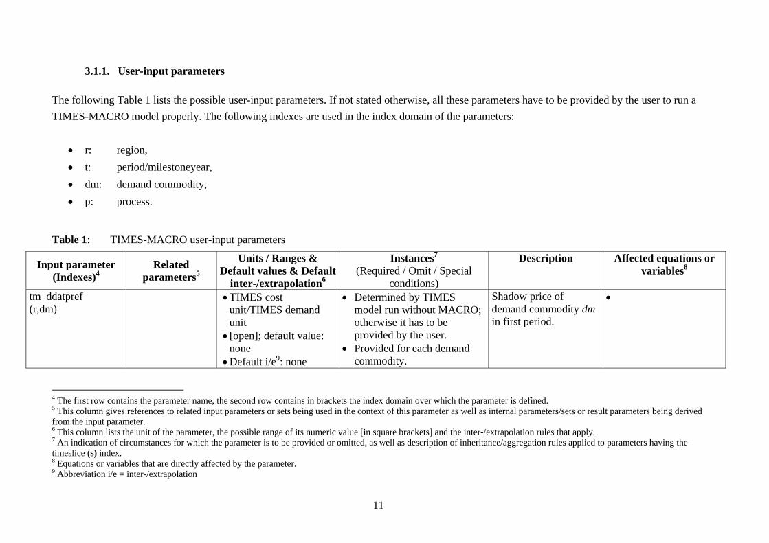
3.1.1. User-input parameters The following Table 1 lists the possible user-input parameters. If not stated otherwise, all these parameters have to be provided by the user to run a TIMES-MACRO model properly. The following indexes are used in the index domain of the parameters:

• r: region, • t: period/milestoneyear, • dm: demand commodity, • p: process.

Table 1: TIMES-MACRO user-input parameters

Input parameter (Indexes)4

Related parameters5

Units / Ranges & Default values & Default

inter-/extrapolation6

Instances7 (Required / Omit / Special

conditions)

Description Affected equations or variables8

tm_ddatpref (r,dm)

• TIMES cost unit/TIMES demand unit

• [open]; default value: none

• Default i/e9: none

• Determined by TIMES model run without MACRO; otherwise it has to be provided by the user.

• Provided for each demand commodity.

Shadow price of demand commodity dm in first period.

•

4 The first row contains the parameter name, the second row contains in brackets the index domain over which the parameter is defined. 5 This column gives references to related input parameters or sets being used in the context of this parameter as well as internal parameters/sets or result parameters being derived from the input parameter. 6 This column lists the unit of the parameter, the possible range of its numeric value [in square brackets] and the inter-/extrapolation rules that apply. 7 An indication of circumstances for which the parameter is to be provided or omitted, as well as description of inheritance/aggregation rules applied to parameters having the timeslice (s) index. 8 Equations or variables that are directly affected by the parameter. 9 Abbreviation i/e = inter-/extrapolation

12


Related parameters5




conditions)


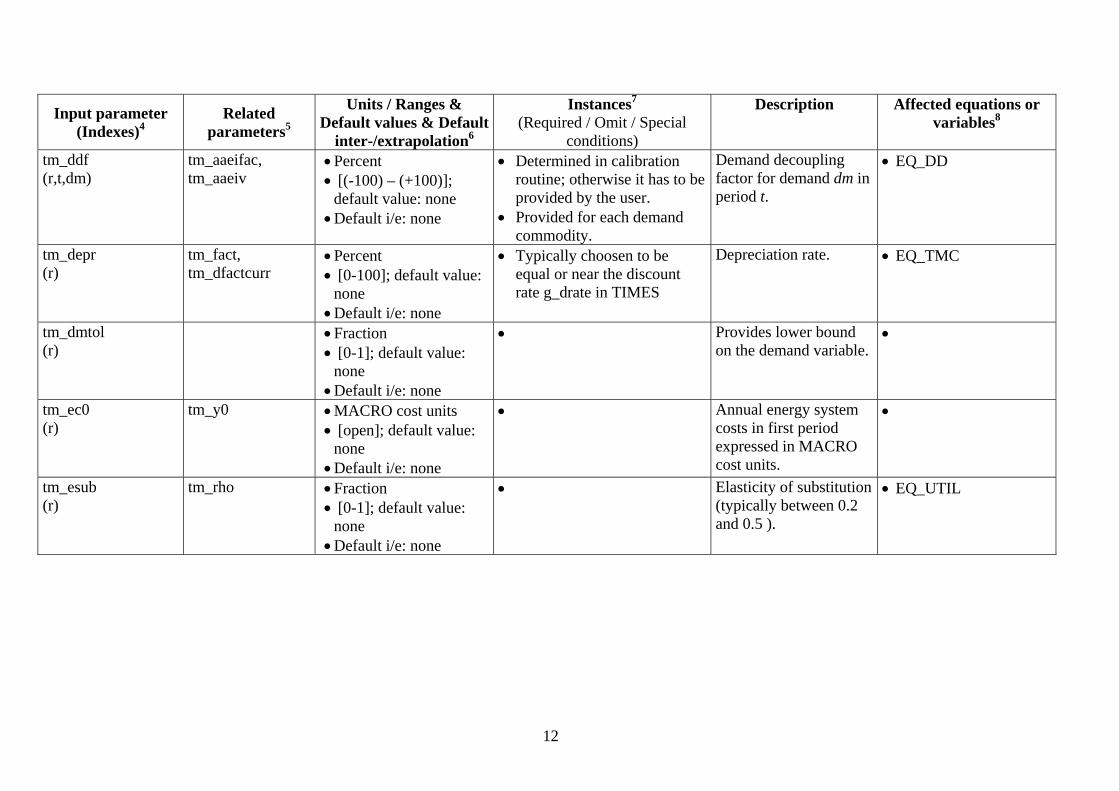
tm_ddf (r,t,dm)

tm_aaeifac, tm_aaeiv

• Percent • [(-100) – (+100)];

default value: none • Default i/e: none

• Determined in calibration routine; otherwise it has to be provided by the user.

• Provided for each demand commodity.

Demand decoupling factor for demand dm in period t.

• EQ_DD

tm_depr (r)

tm_fact, tm_dfactcurr

• Percent • [0-100]; default value:

none • Default i/e: none

• Typically choosen to be equal or near the discount rate g_drate in TIMES

Depreciation rate. • EQ_TMC

tm_dmtol (r)

• Fraction • [0-1]; default value:


• Provides lower bound on the demand variable.

•

tm_ec0 (r)

tm_y0 • MACRO cost units • [open]; default value:


• Annual energy system costs in first period expressed in MACRO cost units.

•

tm_esub (r)

tm_rho • Fraction • [0-1]; default value:


• Elasticity of substitution (typically between 0.2 and 0.5 ).

• EQ_UTIL

13


Related parameters5




conditions)


tm_expbnd (r,t,p)

tm_captb • Units of capacity • [open]; default value:


• To be provided when the market penetration penalty function should be used.

Maximum expansion bound for capacity; used for the cumulated capacity bound tm_captb, above which the penalty is to be applied for new investments in a technology.

• EQ_COSTNRG

tm_expf (r,t)

• Percent • [0-100]; default value:


• To be provided when the market penetration penalty function should be used.

• Internally converted from annual percentage values to period-wise fractions.

Allowed annual capacity expansion factor.

• EQ_COSTNRG • EQ_MPEN

tm_gdp0 (r)

tm_k0, tm_y0 • MACRO cost units • [open]; default value:


• Gross domestic product in first period.

•

tm_gr (r,t)

tm_growv • Percent • [open]; default value:


• It holds the user-defined GDP growth rate and is constant during the calibration procedure, whereas the parameter tm_growv is adjusted throughout the calibration procedure.

Projected annual GDP growth in period t.

•

14


Related parameters5




conditions)


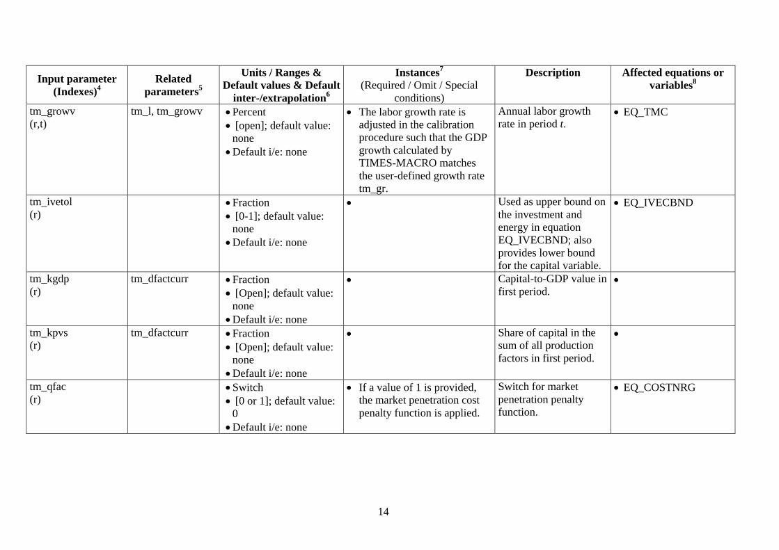
tm_growv (r,t)

tm_l, tm_growv • Percent • [open]; default value:


• The labor growth rate is adjusted in the calibration procedure such that the GDP growth calculated by TIMES-MACRO matches the user-defined growth rate tm_gr.

Annual labor growth rate in period t.

• EQ_TMC

tm_ivetol (r)

• Fraction • [0-1]; default value:


• Used as upper bound on the investment and energy in equation EQ_IVECBND; also provides lower bound for the capital variable.

• EQ_IVECBND

tm_kgdp (r)

tm_dfactcurr • Fraction • [Open]; default value:


• Capital-to-GDP value in first period.

•

tm_kpvs (r)

tm_dfactcurr • Fraction • [Open]; default value:


• Share of capital in the sum of all production factors in first period.

•

tm_qfac (r)

• Switch • [0 or 1]; default value:

0 • Default i/e: none

• If a value of 1 is provided, the market penetration cost penalty function is applied.

Switch for market penetration penalty function.

• EQ_COSTNRG

15


Related parameters5




conditions)


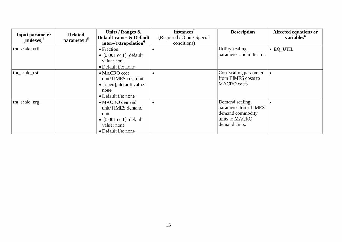
tm_scale_util • Fraction • [0.001 or 1]; default

value: none • Default i/e: none

• Utility scaling parameter and indicator.

• EQ_UTIL

tm_scale_cst • MACRO cost unit/TIMES cost unit


• Default i/e: none

• Cost scaling parameter from TIMES costs to MACRO costs.

•

tm_scale_nrg • MACRO demand unit/TIMES demand unit

• [0.001 or 1]; default value: none


• Demand scaling parameter from TIMES demand commodity units to MACRO demand units.

•

16

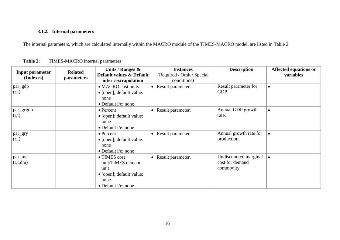
3.1.2. Internal parameters The internal parameters, which are calculated internally within the MACRO module of the TIMES-MACRO model, are listed in Table 2.

Table 2: TIMES-MACRO internal parameters

Input parameter (Indexes)

Related parameters


inter-/extrapolation

Instances (Required / Omit / Special

conditions)

Description Affected equations or variables

par_gdp (r,t)

• MACRO cost units • [open]; default value:


• Result parameter. Result parameter for GDP.

•

par_grgdp (r,t)

• Percent • [open]; default value:


• Result parameter. Annual GDP growth rate.

•

par_gry (r,t)

• Percent • [open]; default value:


• Result parameter. Annual growth rate for production.

•

par_mc (r,t,dm)

• TIMES cost unit/TIMES demand unit



• Result parameter. Undiscounted marginal cost for demand commodity.

•

17


Related parameters




conditions)


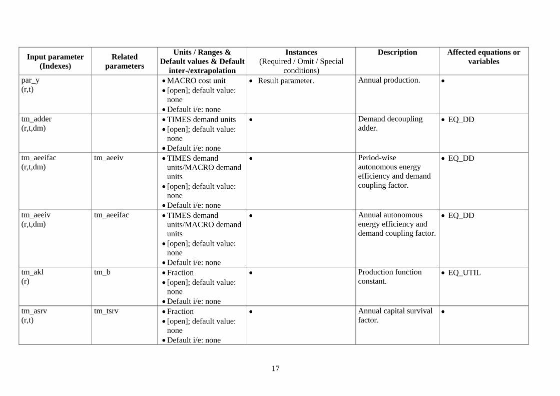
par_y (r,t)

• MACRO cost unit • [open]; default value:


• Result parameter. Annual production. •

tm_adder (r,t,dm)

• TIMES demand units • [open]; default value:


• Demand decoupling adder.

• EQ_DD

tm_aeeifac (r,t,dm)

tm_aeeiv • TIMES demand units/MACRO demand units



• Period-wise autonomous energy efficiency and demand coupling factor.

• EQ_DD

tm_aeeiv (r,t,dm)

tm_aeeifac • TIMES demand units/MACRO demand units



• Annual autonomous energy efficiency and demand coupling factor.

• EQ_DD

tm_akl (r)

tm_b • Fraction • [open]; default value:


• Production function constant.

• EQ_UTIL

tm_asrv (r,t)

tm_tsrv • Fraction • [open]; default value:


• Annual capital survival factor.

•

18


Related parameters




conditions)


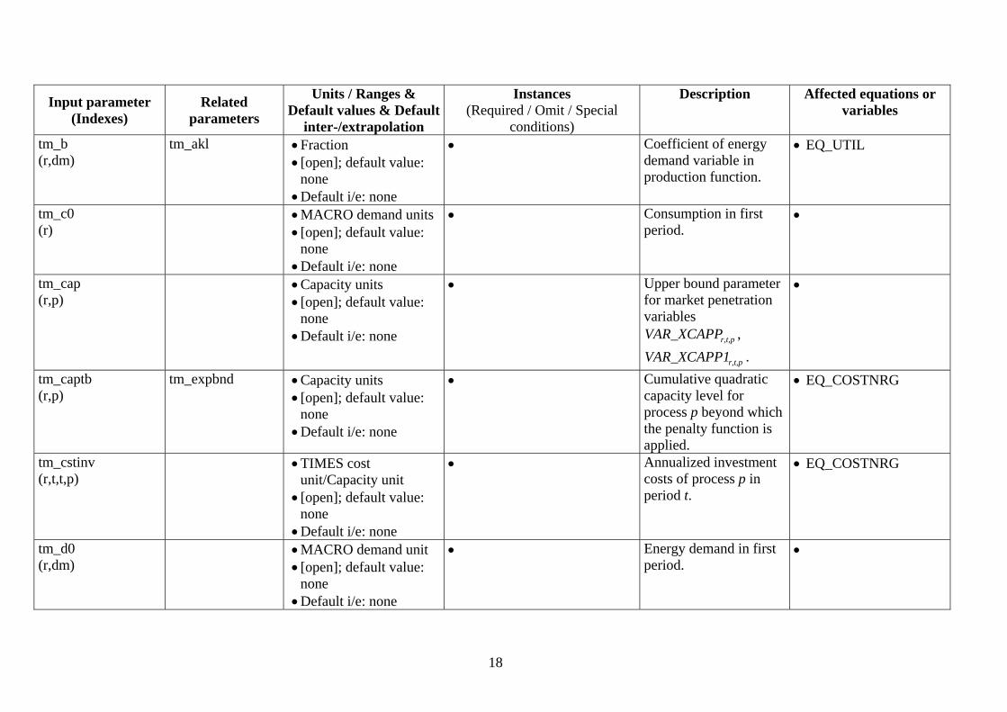
tm_b (r,dm)

tm_akl • Fraction • [open]; default value:


• Coefficient of energy demand variable in production function.

• EQ_UTIL

tm_c0 (r)

• MACRO demand units • [open]; default value:


• Consumption in first period.

•

tm_cap (r,p)

• Capacity units • [open]; default value:


• Upper bound parameter for market penetration variables

r,t,pVAR_XCAPP ,

r,t,pVAR_XCAPP1 .

•

tm_captb (r,p)

tm_expbnd • Capacity units • [open]; default value:


• Cumulative quadratic capacity level for process p beyond which the penalty function is applied.

• EQ_COSTNRG

tm_cstinv (r,t,t,p)

• TIMES cost unit/Capacity unit



• Annualized investment costs of process p in period t.

• EQ_COSTNRG

tm_d0 (r,dm)

• MACRO demand unit • [open]; default value:


• Energy demand in first period.

•

19


Related parameters




conditions)


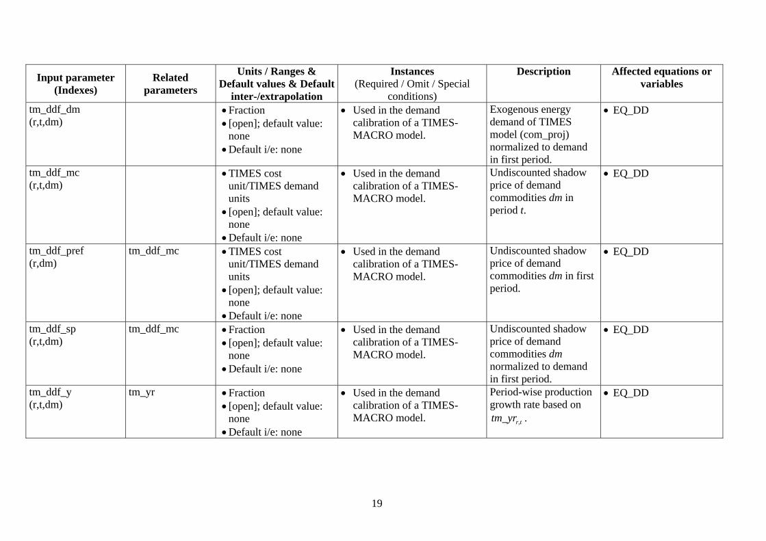
tm_ddf_dm (r,t,dm)

• Fraction • [open]; default value:


• Used in the demand calibration of a TIMES-MACRO model.

Exogenous energy demand of TIMES model (com_proj) normalized to demand in first period.

• EQ_DD

tm_ddf_mc (r,t,dm)

• TIMES cost unit/TIMES demand units




Undiscounted shadow price of demand commodities dm in period t.

• EQ_DD

tm_ddf_pref (r,dm)

tm_ddf_mc • TIMES cost unit/TIMES demand units




Undiscounted shadow price of demand commodities dm in first period.

• EQ_DD

tm_ddf_sp (r,t,dm)

tm_ddf_mc • Fraction • [open]; default value:



Undiscounted shadow price of demand commodities dm normalized to demand in first period.

• EQ_DD

tm_ddf_y (r,t,dm)

tm_yr • Fraction • [open]; default value:



Period-wise production growth rate based on

r,ttm_yr .

• EQ_DD

20


Related parameters




conditions)


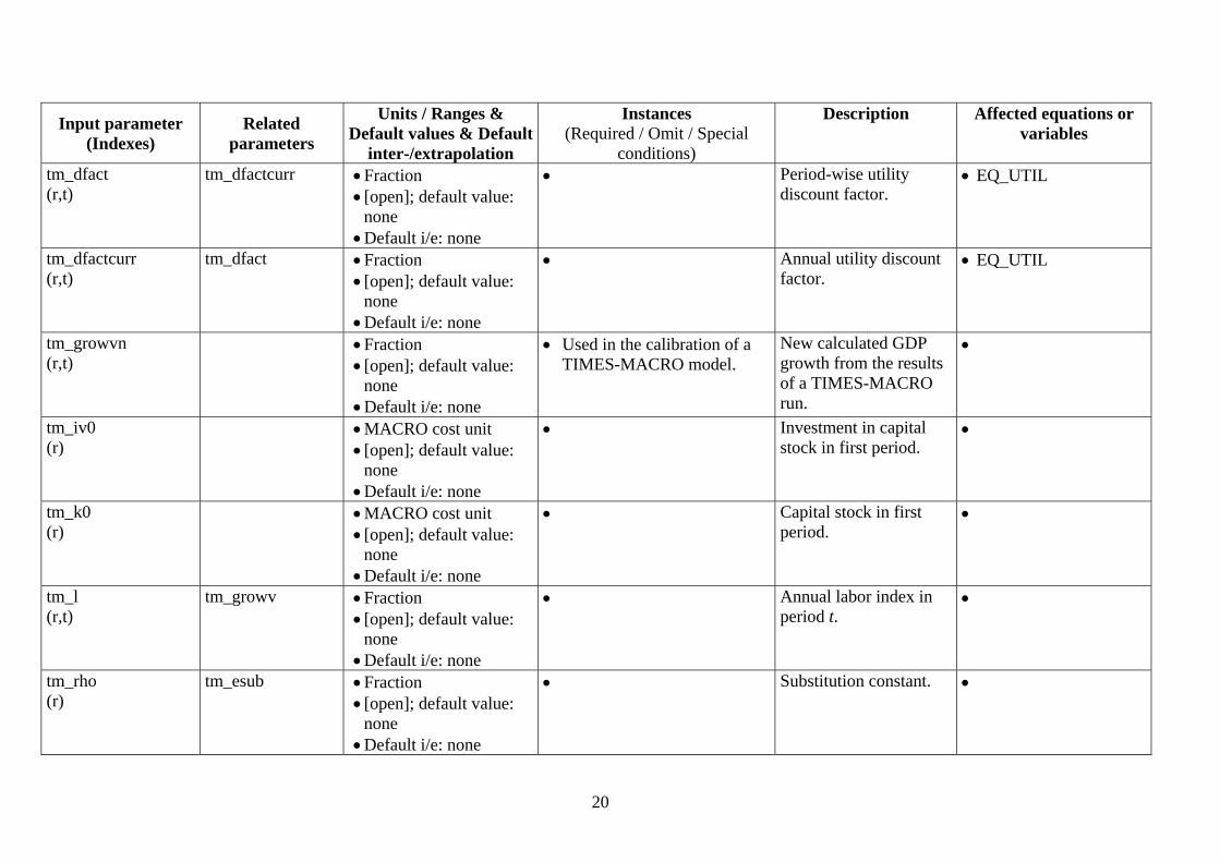
tm_dfact (r,t)

tm_dfactcurr • Fraction • [open]; default value:


• Period-wise utility discount factor.

• EQ_UTIL

tm_dfactcurr (r,t)

tm_dfact • Fraction • [open]; default value:


• Annual utility discount factor.

• EQ_UTIL

tm_growvn (r,t)

• Fraction • [open]; default value:


• Used in the calibration of a TIMES-MACRO model.

New calculated GDP growth from the results of a TIMES-MACRO run.

•

tm_iv0 (r)



• Investment in capital stock in first period.

•

tm_k0 (r)



• Capital stock in first period.

•

tm_l (r,t)

tm_growv • Fraction • [open]; default value:


• Annual labor index in period t.

•

tm_rho (r)

tm_esub • Fraction • [open]; default value:


• Substitution constant. •

21


Related parameters




conditions)


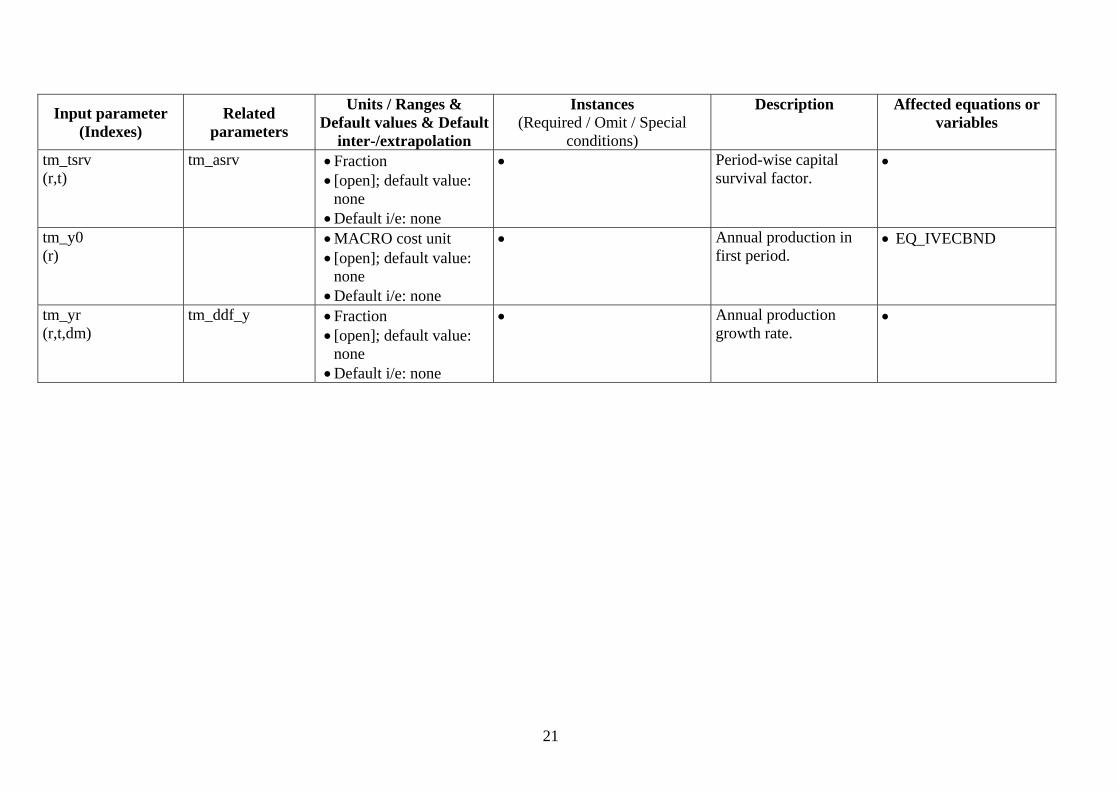
tm_tsrv (r,t)

tm_asrv • Fraction • [open]; default value:


• Period-wise capital survival factor.

•

tm_y0 (r)



• Annual production in first period.

• EQ_IVECBND

tm_yr (r,t,dm)

tm_ddf_y • Fraction • [open]; default value:


• Annual production growth rate.

•

22

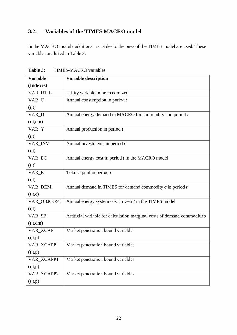
3.2. Variables of the TIMES MACRO model In the MACRO module additional variables to the ones of the TIMES model are used. These variables are listed in Table 3.

Table 3: TIMES-MACRO variables

Variable (Indexes)

Variable description

VAR_UTIL Utility variable to be maximized VAR_C (r,t)

Annual consumption in period t

VAR_D (r,t,dm)

Annual energy demand in MACRO for commodity c in period t

VAR_Y (r,t)

Annual production in period t

VAR_INV (r,t)

Annual investments in period t

VAR_EC (r,t)

Annual energy cost in period t in the MACRO model

VAR_K (r,t)

Total capital in period t

VAR_DEM (r,t,c)

Annual demand in TIMES for demand commodity c in period t

VAR_OBJCOST (r,t)

Annual energy system cost in year t in the TIMES model

VAR_SP (r,t,dm)

Artificial variable for calculation marginal costs of demand commodities

VAR_XCAP (r,t,p)

Market penetration bound variables

VAR_XCAPP (r,t,p)


VAR_XCAPP1 (r,t,p)


VAR_XCAPP2 (r,t,p)


23

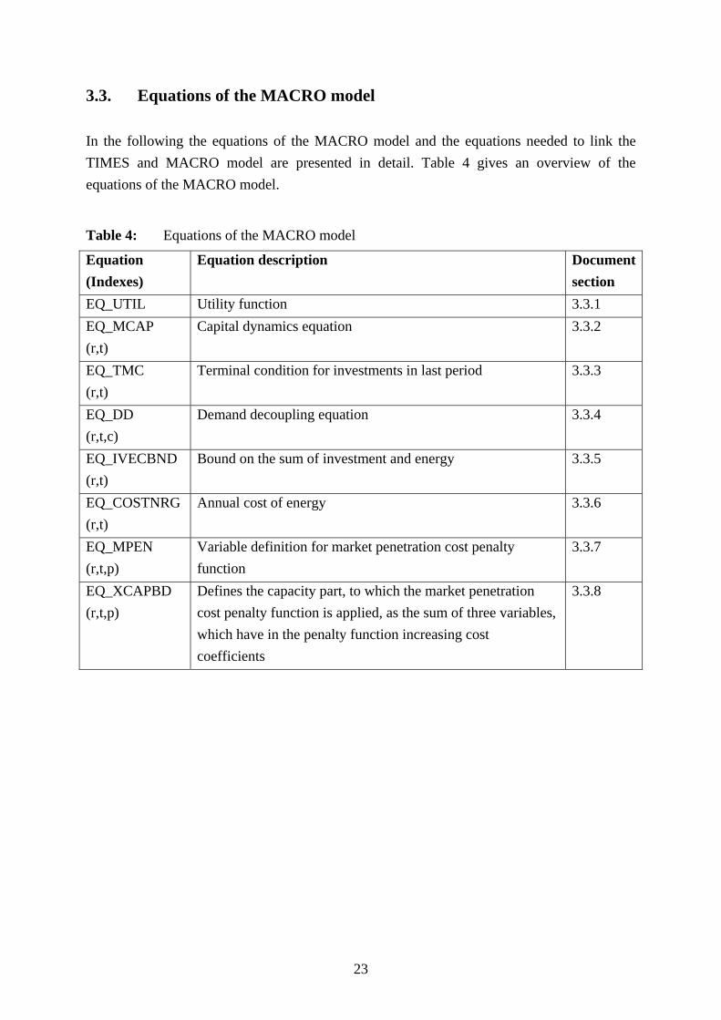
3.3. Equations of the MACRO model In the following the equations of the MACRO model and the equations needed to link the TIMES and MACRO model are presented in detail. Table 4 gives an overview of the equations of the MACRO model.

Table 4: Equations of the MACRO model

Equation (Indexes)

Equation description Document section

EQ_UTIL Utility function 3.3.1 EQ_MCAP (r,t)

Capital dynamics equation 3.3.2

EQ_TMC (r,t)

Terminal condition for investments in last period 3.3.3

EQ_DD (r,t,c)

Demand decoupling equation 3.3.4

EQ_IVECBND (r,t)

Bound on the sum of investment and energy 3.3.5

EQ_COSTNRG (r,t)

Annual cost of energy 3.3.6

EQ_MPEN (r,t,p)

Variable definition for market penetration cost penalty function

3.3.7

EQ_XCAPBD (r,t,p)

Defines the capacity part, to which the market penetration cost penalty function is applied, as the sum of three variables, which have in the penalty function increasing cost coefficients

3.3.8

24

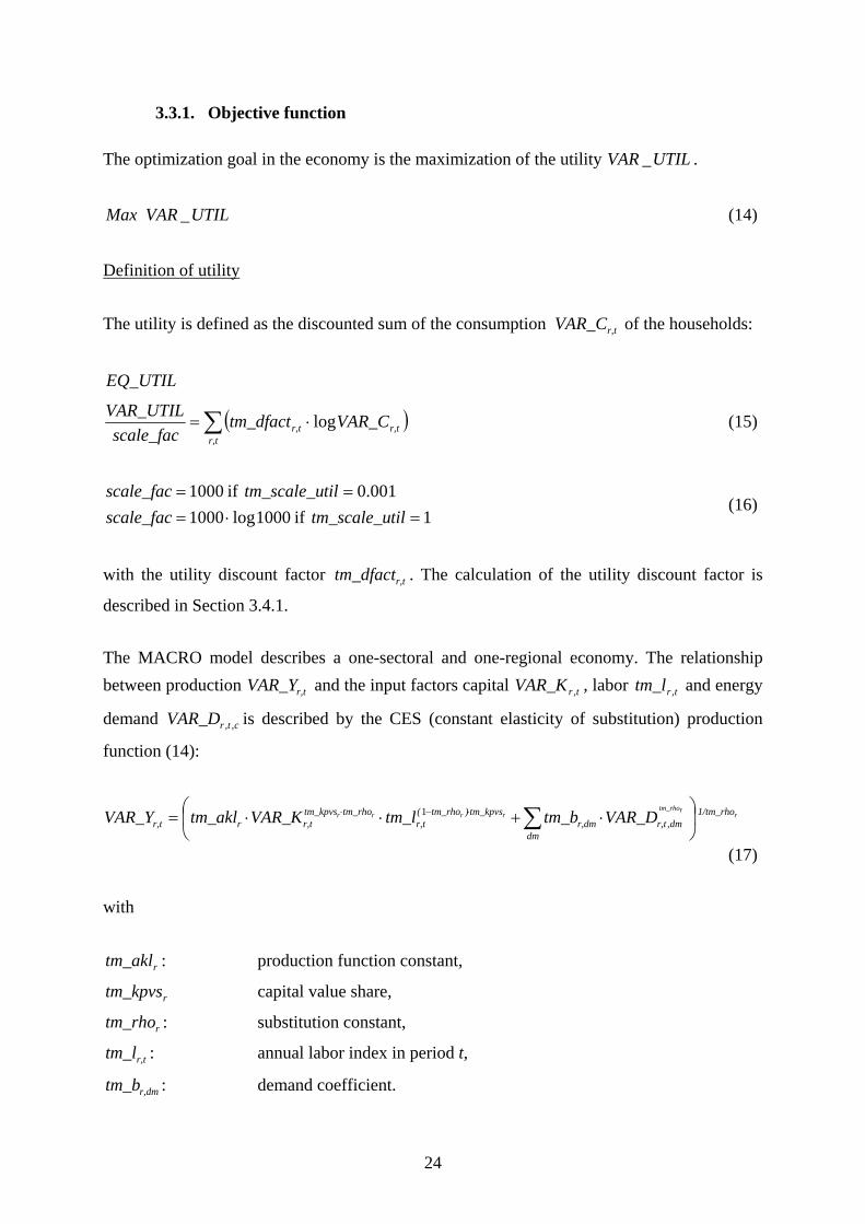
3.3.1. Objective function The optimization goal in the economy is the maximization of the utility UTILVAR _ .

UTILVARMax _ (14)

Definition of utility The utility is defined as the discounted sum of the consumption r,tVAR_C of the households:

EQ_UTIL

( )∑ ⋅=r,t

r,tr,t VAR_Ctm_dfactscale_fac

VAR_UTIL log (15)

1if1000log1000001.0if1000

=⋅===

tiltm_scale_uscale_factiltm_scale_uscale_fac

(16)

with the utility discount factor r,ttm_dfact . The calculation of the utility discount factor is

described in Section 3.4.1. The MACRO model describes a one-sectoral and one-regional economy. The relationship between production r,tVAR_Y and the input factors capital trVAR_K , , labor trtm_l , and energy

demand ctrVAR_D ,, is described by the CES (constant elasticity of substitution) production

function (14):

rrtm_rho

rrrr 1/tm_rho

dmdmr,tr,dm

tm_kpvs)tm_rho(r,t

tm_rhotm_kpvsr,trr,t VAR_Dtm_btm_lVAR_Ktm_aklVAR_Y ⎟

⎠

⎞⎜⎝

⎛⋅+⋅⋅= ∑⋅−⋅

,1

(17) with

rtm_akl : production function constant,

rtm_kpvs capital value share,

rtm_rho : substitution constant,

r,ttm_l : annual labor index in period t,

r,dmtm_b : demand coefficient.

25

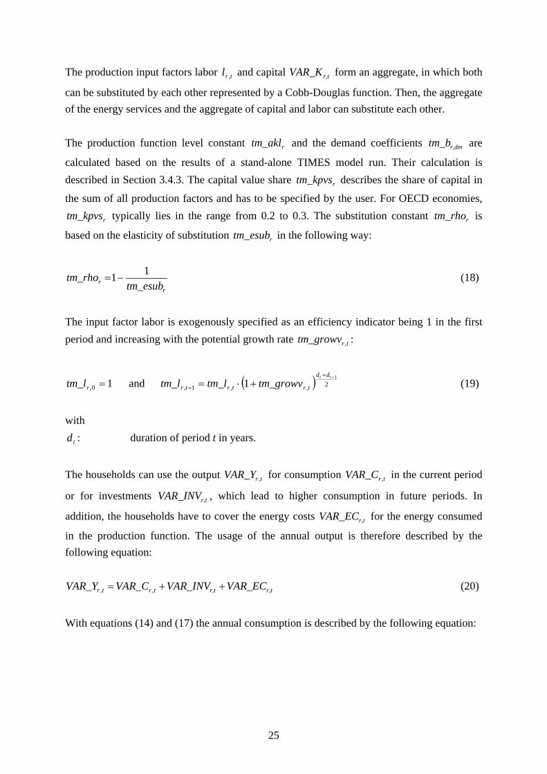
The production input factors labor trl , and capital r,tVAR_K form an aggregate, in which both

can be substituted by each other represented by a Cobb-Douglas function. Then, the aggregate of the energy services and the aggregate of capital and labor can substitute each other. The production function level constant rtm_akl and the demand coefficients r,dmtm_b are

calculated based on the results of a stand-alone TIMES model run. Their calculation is described in Section 3.4.3. The capital value share rtm_kpvs describes the share of capital in

the sum of all production factors and has to be specified by the user. For OECD economies,

rtm_kpvs typically lies in the range from 0.2 to 0.3. The substitution constant rtm_rho is

based on the elasticity of substitution rtm_esub in the following way:

rr tm_esub

tm_rho 11−= (18)

The input factor labor is exogenously specified as an efficiency indicator being 1 in the first period and increasing with the potential growth rate trtm_growv , :

( ) 2,,1,0,

1

1 and1++

+ +⋅==tt dd

trtrtrr tm_growvtm_ltm_ltm_l (19)

with

td : duration of period t in years.

The households can use the output trVAR_Y , for consumption trVAR_C , in the current period

or for investments r,tVAR_INV , which lead to higher consumption in future periods. In

addition, the households have to cover the energy costs r,tVAR_EC for the energy consumed

in the production function. The usage of the annual output is therefore described by the following equation:

r,tr,ttrtr VAR_ECVAR_INVVAR_CVAR_Y ++= ,, (20)

With equations (14) and (17) the annual consumption is described by the following equation:

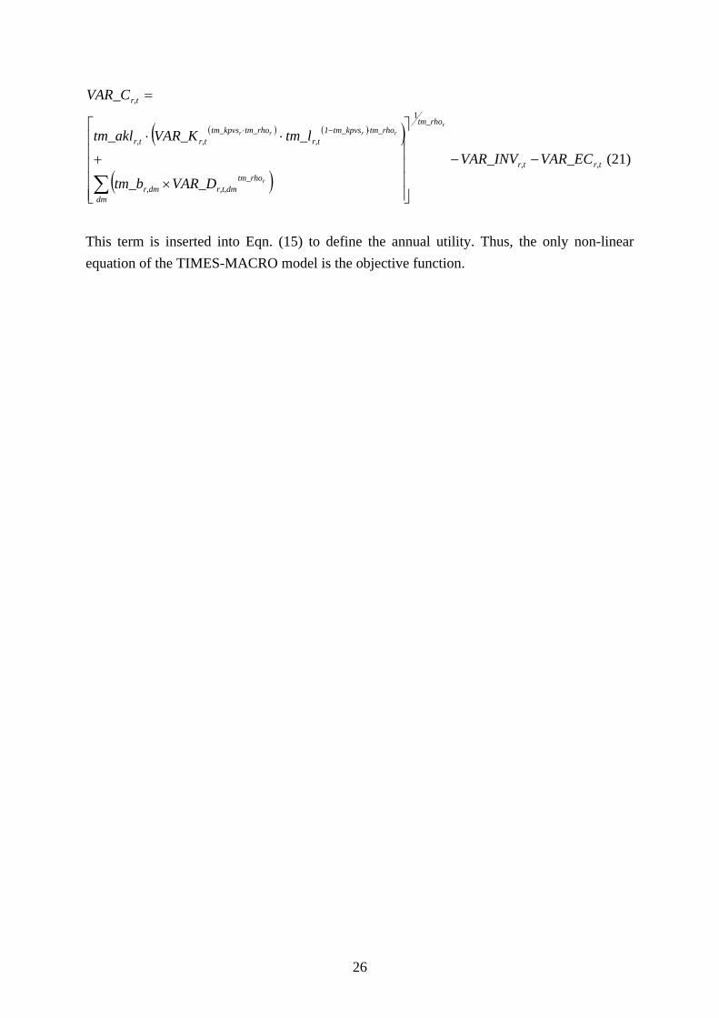
26

( ) ( )( )

( )r,tr,t

tm_rho

dm

tm_rhor,t,dmr,dm

tm_rhotm_kpvs1r,t

tm_rhotm_kpvsr,tr,t

r,t

VAR_ECVAR_INV

VAR_Dtm_b

tm_lVAR_Ktm_akl

VAR_C

r

r

rrrr

−−

⎥⎥⎥⎥⎥

⎦

⎤

⎢⎢⎢⎢⎢

⎣

⎡

×

+

⋅⋅

=

∑

⋅−⋅

1

(21)

This term is inserted into Eqn. (15) to define the annual utility. Thus, the only non-linear equation of the TIMES-MACRO model is the objective function.

27

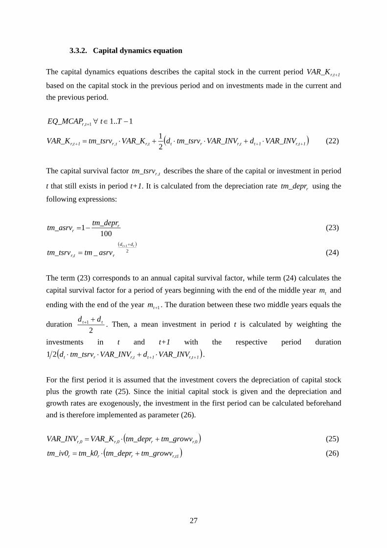
3.3.2. Capital dynamics equation The capital dynamics equations describes the capital stock in the current period 1r,tVAR_K +

based on the capital stock in the previous period and on investments made in the current and the previous period.

1, +trEQ_MCAP 1..1 −∈∀ Tt

( )1r,t1tr,trtr,ttr1r,t VAR_INVdVAR_INVtm_tsrvdVAR_Ktm_tsrvVAR_K +++ ⋅+⋅⋅+⋅=21

, (22)

The capital survival factor trtm_tsrv , describes the share of the capital or investment in period

t that still exists in period t+1. It is calculated from the depreciation rate rtm_depr using the

following expressions:

1001 r

rtm_deprtm_asrv −= (23)

( )21

_tt dd

rr,t asrvtmtm_tsrv++

= (24)

The term (23) corresponds to an annual capital survival factor, while term (24) calculates the capital survival factor for a period of years beginning with the end of the middle year tm and

ending with the end of the year 1+tm . The duration between these two middle years equals the

duration 2

1 tt dd ++ . Then, a mean investment in period t is calculated by weighting the

investments in t and t+1 with the respective period duration ( )1r,t1tr,trt VAR_INVdVAR_INVtm_tsrvd ++ ⋅+⋅⋅21 .

For the first period it is assumed that the investment covers the depreciation of capital stock plus the growth rate (25). Since the initial capital stock is given and the depreciation and growth rates are exogenously, the investment in the first period can be calculated beforehand and is therefore implemented as parameter (26).

( )0r,rr,0r,0 tm_growvtm_deprVAR_KVAR_INV +⋅= (25)

( )r,t1rrr tm_growvtm_deprtm_k0tm_iv0 +⋅= (26)

28

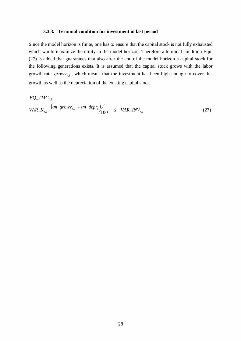
3.3.3. Terminal condition for investment in last period Since the model horizon is finite, one has to ensure that the capital stock is not fully exhausted which would maximize the utility in the model horizon. Therefore a terminal condition Eqn. (27) is added that guarantees that also after the end of the model horizon a capital stock for the following generations exists. It is assumed that the capital stock grows with the labor growth rate Trgrowv , , which means that the investment has been high enough to cover this

growth as well as the depreciation of the existing capital stock.

TrEQ_TMC ,

( )Tr

rTrr,T VAR_INVtm_deprtm_growvVAR_K ,

,100 ≤+⋅ (27)

29

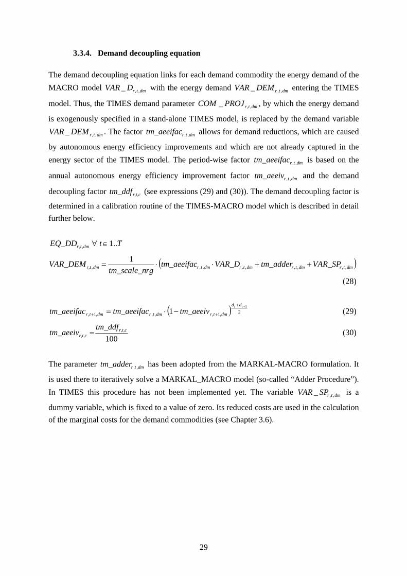
3.3.4. Demand decoupling equation The demand decoupling equation links for each demand commodity the energy demand of the MACRO model dmtrDVAR ,,_ with the energy demand dmtrDEMVAR ,,_ entering the TIMES

model. Thus, the TIMES demand parameter dmtrPROJCOM ,,_ , by which the energy demand

is exogenously specified in a stand-alone TIMES model, is replaced by the demand variable

dmtrDEMVAR ,,_ . The factor dmtrtm_aeeifac ,, allows for demand reductions, which are caused

by autonomous energy efficiency improvements and which are not already captured in the energy sector of the TIMES model. The period-wise factor dmtrtm_aeeifac ,, is based on the

annual autonomous energy efficiency improvement factor dmtrtm_aeeiv ,, and the demand

decoupling factor r,t,ctm_ddf (see expressions (29) and (30)). The demand decoupling factor is

determined in a calibration routine of the TIMES-MACRO model which is described in detail further below.

dmtrEQ_DD ,, Tt ..1∈∀

( )dmtrdmtrdmtrdmtrdmr,t VAR_SPtm_adderVAR_Dtm_aeeifacrgtm_scale_n

VAR_DEM ,,,,,,,,,1

++⋅⋅=

(28)

( ) 2,1,,,,1,

1

1++

++ −⋅=tt dd

dmtrdmtrdmtr tm_aeeivtm_aeeifactm_aeeifac (29)

100r,t,c

r,t,ctm_ddf

tm_aeeiv = (30)

The parameter dmtrtm_adder ,, has been adopted from the MARKAL-MACRO formulation. It

is used there to iteratively solve a MARKAL_MACRO model (so-called “Adder Procedure”). In TIMES this procedure has not been implemented yet. The variable dmtrSPVAR ,,_ is a

dummy variable, which is fixed to a value of zero. Its reduced costs are used in the calculation of the marginal costs for the demand commodities (see Chapter 3.6).

30

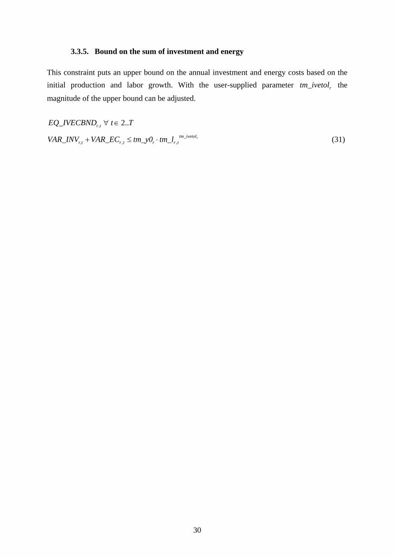
3.3.5. Bound on the sum of investment and energy This constraint puts an upper bound on the annual investment and energy costs based on the initial production and labor growth. With the user-supplied parameter rtm_ivetol the

magnitude of the upper bound can be adjusted.

trEQ_IVECBND , Tt ..2∈∀

rtm_ivetoltrrtrr,t tm_ltm_y0VAR_ECVAR_INV ,, ⋅≤+ (31)

31

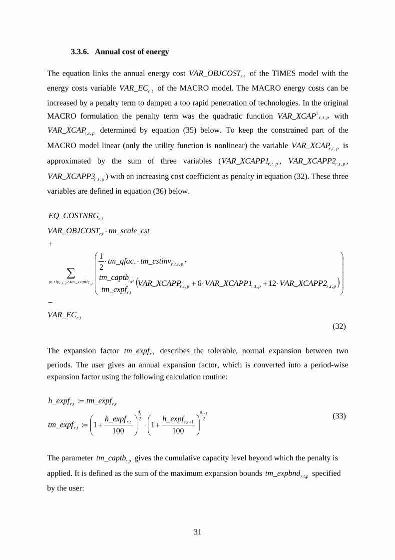
3.3.6. Annual cost of energy The equation links the annual energy cost r,tTVAR_OBJCOS of the TIMES model with the

energy costs variable trVAR_EC , of the MACRO model. The MACRO energy costs can be

increased by a penalty term to dampen a too rapid penetration of technologies. In the original

MACRO formulation the penalty term was the quadratic function ptrVAR_XCAP ,,2 with

ptrVAR_XCAP ,, determined by equation (35) below. To keep the constrained part of the

MACRO model linear (only the utility function is nonlinear) the variable ptrVAR_XCAP ,, is

approximated by the sum of three variables ( ptrVAR_XCAPP1 ,, , ptrVAR_XCAPP2 ,, ,

ptrVAR_XCAPP3 ,, ) with an increasing cost coefficient as penalty in equation (32). These three

variables are defined in equation (36) below.

trEQ_COSTNRG ,

( )

tr

captbtmrtppptrptrptr

r,t

r,p

pttrr

r,t

VAR_EC

VAR_XCAPP2VAR_XCAPP1VAR_XCAPPtm_expf

tm_captb

tm_cstinvtm_qfac

sttm_scale_cTVAR_OBJCOS

prptr

,

_,,,,,,

,,,

,,, 126

21

=

⎟⎟⎟⎟

⎠

⎞

⎜⎜⎜⎜

⎝

⎛

⋅+⋅+

⋅⋅⋅

+

⋅

∑∧∈

(32) The expansion factor r,ttm_expf describes the tolerable, normal expansion between two

periods. The user gives an annual expansion factor, which is converted into a period-wise expansion factor using the following calculation routine:

21

21

1001

1001:

:+

⎟⎟⎠

⎞⎜⎜⎝

⎛+⋅⎟⎟

⎠

⎞⎜⎜⎝

⎛+=

=

+

tt d

r,t

d

r,tr,t

r,tr,t

h_expfh_expftm_expf

tm_expfh_expf

(33)

The parameter r,ptm_captb gives the cumulative capacity level beyond which the penalty is

applied. It is defined as the sum of the maximum expansion bounds r,t,ptm_expbnd specified

by the user:

32

∑∈

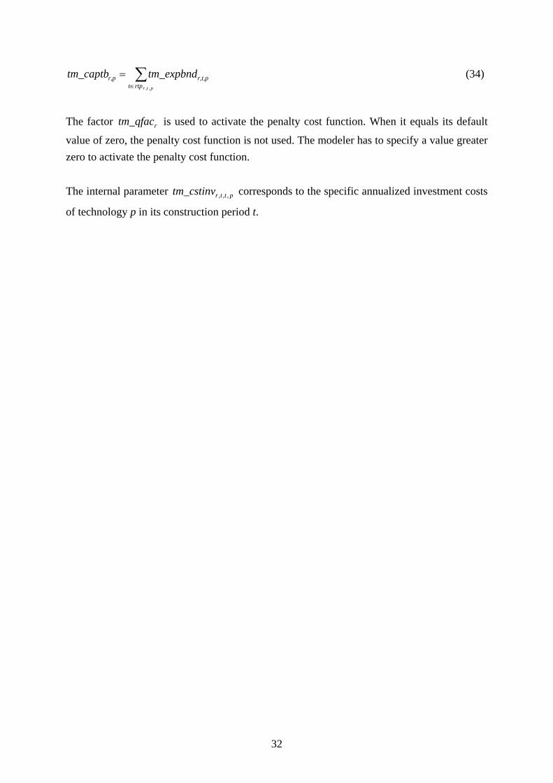
=ptrrtpt

r,t,pr,p tm_expbndtm_captb,,

(34)

The factor rtm_qfac is used to activate the penalty cost function. When it equals its default

value of zero, the penalty cost function is not used. The modeler has to specify a value greater zero to activate the penalty cost function. The internal parameter pttrtm_cstinv ,,, corresponds to the specific annualized investment costs

of technology p in its construction period t.

33

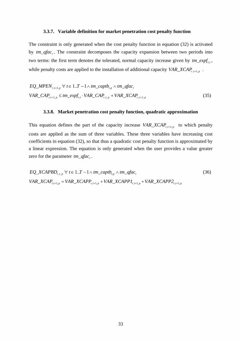
3.3.7. Variable definition for market penetration cost penalty function The constraint is only generated when the cost penalty function in equation (32) is activated by rtm_qfac . The constraint decomposes the capacity expansion between two periods into

two terms: the first term denotes the tolerated, normal capacity increase given by r,ttm_expf ,

while penalty costs are applied to the installation of additional capacity ptrVAR_XCAP ,1, + .

ptrEQ_MPEN ,1, + rr,p tm_qfactm_captbTt ∧∧−∈∀ 1..1

ptrptrr,tpr,t VAR_XCAPVAR_CAPtm_expfVAR_CAP ,1,,,,1 ++ +⋅≤ (35)

3.3.8. Market penetration cost penalty function, quadratic approximation

This equation defines the part of the capacity increase ptrVAR_XCAP ,1, + to which penalty

costs are applied as the sum of three variables. These three variables have increasing cost coefficients in equation (32), so that thus a quadratic cost penalty function is approximated by a linear expression. The equation is only generated when the user provides a value greater zero for the parameter rtm_qfac .

ptrEQ_XCAPBD ,, rr,p tm_qfactm_captbTt ∧∧−∈∀ 1..1 (36)

ptrptrptrpr,t VAR_XCAPP2VAR_XCAPP1VAR_XCAPPVAR_XCAP ,1,,1,,1,,1 ++++ ++=

34

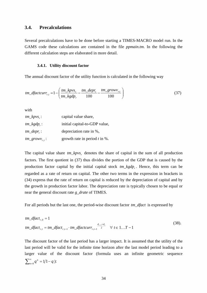
3.4. Precalculations Several precalculations have to be done before starting a TIMES-MACRO model run. In the GAMS code these calculations are contained in the file ppmain.tm. In the following the different calculation steps are elaborated in more detail.

3.4.1. Utility discount factor The annual discount factor of the utility function is calculated in the following way

⎟⎟⎠

⎞⎜⎜⎝

⎛−−−=

1001001,

r,tr

r

rtr

tm_growvtm_deprtm_kgdptm_kpvsrrtm_dfactcu (37)

with

rtm_kpvs : capital value share,

rtm_kgdp : initial capital-to-GDP value,

rtm_depr : depreciation rate in %,

trtm_growv , : growth rate in period t in %.

The capital value share rtm_kpvs denotes the share of capital in the sum of all production

factors. The first quotient in (37) thus divides the portion of the GDP that is caused by the production factor capital by the initial capital stock rtm_kgdp . Hence, this term can be

regarded as a rate of return on capital. The other two terms in the expression in brackets in (34) express that the rate of return on capital is reduced by the depreciation of capital and by the growth in production factor labor. The depreciation rate is typically chosen to be equal or near the general discount rate g_drate of TIMES. For all periods but the last one, the period-wise discount factor tm_dfact is expressed by

11

1

21,1,,

0,

1

−∈∀⋅=

=+

−−

−

Ttrrtm_dfactcutm_dfacttm_dfact

tm_dfacttt dd

trtrtr

r

K (38).

The discount factor of the last period has a larger impact. It is assumed that the utility of the last period will be valid for the infinite time horizon after the last model period leading to a larger value of the discount factor (formula uses an infinite geometric sequence

∑∞

=−=

011

nn qq ):

35

2,

21,1,, 1

1

1TT

TT

dd

Tr

dd

TrTrTr

rrtm_dfactcu

rrtm_dfactcutm_dfacttm_dfact +

+

−−

−

−

−

⋅= (39).

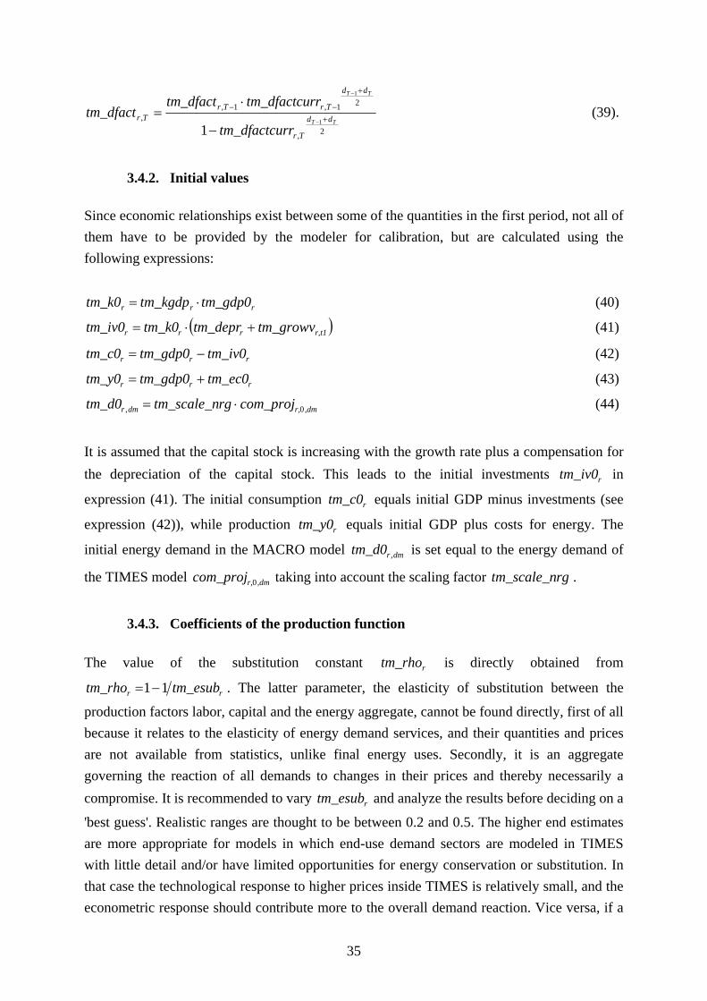
3.4.2. Initial values

Since economic relationships exist between some of the quantities in the first period, not all of them have to be provided by the modeler for calibration, but are calculated using the following expressions:

rrr tm_gdp0tm_kgdptm_k0 ⋅= (40)

( )r,t1rrr tm_growvtm_deprtm_k0tm_iv0 +⋅= (41)

rrr tm_iv0tm_gdp0tm_c0 −= (42)

rrr tm_ec0tm_gdp0tm_y0 += (43)

,dmr,dmr com_projrgtm_scale_ntm_d0 0, ⋅= (44)

It is assumed that the capital stock is increasing with the growth rate plus a compensation for the depreciation of the capital stock. This leads to the initial investments rtm_iv0 in

expression (41). The initial consumption rtm_c0 equals initial GDP minus investments (see

expression (42)), while production rtm_y0 equals initial GDP plus costs for energy. The

initial energy demand in the MACRO model dmrtm_d0 , is set equal to the energy demand of

the TIMES model ,dmr,com_proj 0 taking into account the scaling factor rgtm_scale_n .

3.4.3. Coefficients of the production function

The value of the substitution constant rtm_rho is directly obtained from

rr tm_esubtm_rho 11−= . The latter parameter, the elasticity of substitution between the

production factors labor, capital and the energy aggregate, cannot be found directly, first of all because it relates to the elasticity of energy demand services, and their quantities and prices are not available from statistics, unlike final energy uses. Secondly, it is an aggregate governing the reaction of all demands to changes in their prices and thereby necessarily a compromise. It is recommended to vary rtm_esub and analyze the results before deciding on a

'best guess'. Realistic ranges are thought to be between 0.2 and 0.5. The higher end estimates are more appropriate for models in which end-use demand sectors are modeled in TIMES with little detail and/or have limited opportunities for energy conservation or substitution. In that case the technological response to higher prices inside TIMES is relatively small, and the econometric response should contribute more to the overall demand reaction. Vice versa, if a

36

large number of technological response options are present in TIMES, rtm_esub should be at

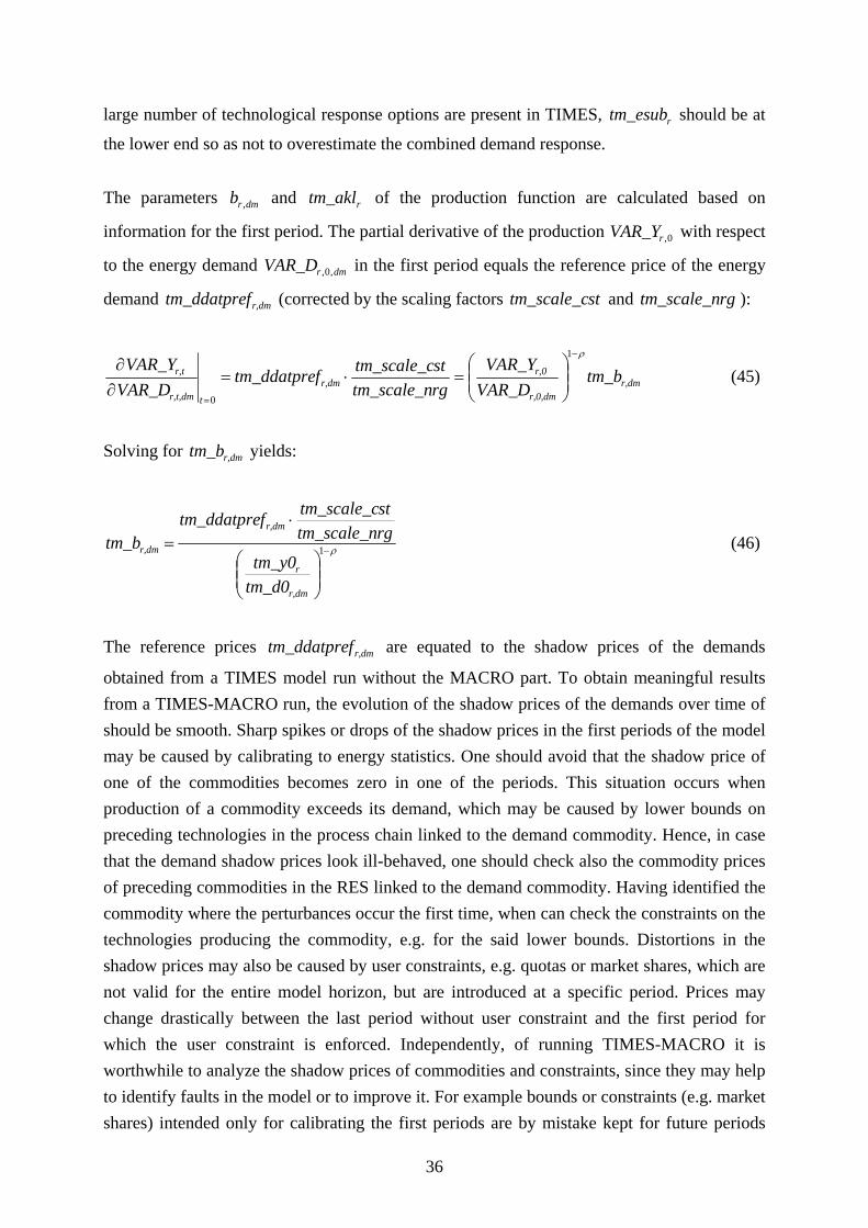
the lower end so as not to overestimate the combined demand response. The parameters dmrb , and rtm_akl of the production function are calculated based on

information for the first period. The partial derivative of the production 0,rVAR_Y with respect

to the energy demand dmrVAR_D ,0, in the first period equals the reference price of the energy

demand r,dmftm_ddatpre (corrected by the scaling factors sttm_scale_c and rgtm_scale_n ):

r,dmr,0,dm

r,0r,dm

tr,t,dm

r,t tm_bVAR_D

VAR_Yrgtm_scale_nsttm_scale_cftm_ddatpre

VAR_DVAR_Y

ρ−

=⎟⎟⎠

⎞⎜⎜⎝

⎛=⋅=

∂∂

1

0

(45)

Solving for r,dmtm_b yields:

ρ−

⎟⎟⎠

⎞⎜⎜⎝

⎛

⋅= 1

r,dm

r

r,dm

r,dm

tm_d0tm_y0

rgtm_scale_nsttm_scale_cftm_ddatpre

tm_b (46)

The reference prices r,dmftm_ddatpre are equated to the shadow prices of the demands

obtained from a TIMES model run without the MACRO part. To obtain meaningful results from a TIMES-MACRO run, the evolution of the shadow prices of the demands over time of should be smooth. Sharp spikes or drops of the shadow prices in the first periods of the model may be caused by calibrating to energy statistics. One should avoid that the shadow price of one of the commodities becomes zero in one of the periods. This situation occurs when production of a commodity exceeds its demand, which may be caused by lower bounds on preceding technologies in the process chain linked to the demand commodity. Hence, in case that the demand shadow prices look ill-behaved, one should check also the commodity prices of preceding commodities in the RES linked to the demand commodity. Having identified the commodity where the perturbances occur the first time, when can check the constraints on the technologies producing the commodity, e.g. for the said lower bounds. Distortions in the shadow prices may also be caused by user constraints, e.g. quotas or market shares, which are not valid for the entire model horizon, but are introduced at a specific period. Prices may change drastically between the last period without user constraint and the first period for which the user constraint is enforced. Independently, of running TIMES-MACRO it is worthwhile to analyze the shadow prices of commodities and constraints, since they may help to identify faults in the model or to improve it. For example bounds or constraints (e.g. market shares) intended only for calibrating the first periods are by mistake kept for future periods

37

limiting the flexibility of the model when new policies, e.g. GHG reduction targets, are introduced. Knowing dmrbtm ,_ the production function constant rtm_akl can be definite by solving the

production function (11) in the initial period for rtm_akl :

rr

rr

tm_rhotm_kpvsr

dm

tm_rhor,dmr,dm

tm_rhor

r tm_k0

tm_d0tm_btm_y0tm_akl ⋅

∑ ⋅−= (47)

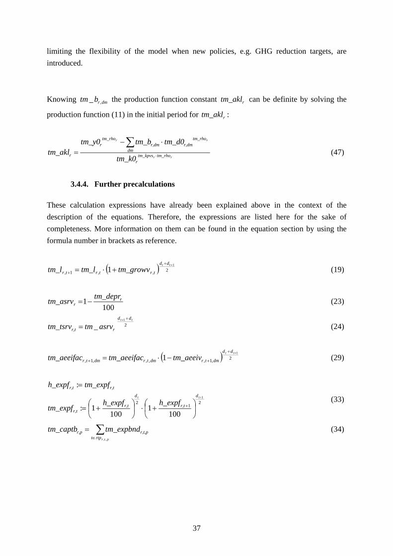
3.4.4. Further precalculations

These calculation expressions have already been explained above in the context of the description of the equations. Therefore, the expressions are listed here for the sake of completeness. More information on them can be found in the equation section by using the formula number in brackets as reference.

( ) 2,,1,

1

1++

+ +⋅=tt dd

trtrtr tm_growvtm_ltm_l (19)

1001 r

rtm_deprtm_asrv −= (23)

21

_tt dd

rr,t asrvtmtm_tsrv++

= (24)

( ) 2,1,,,,1,

1

1++

++ −⋅=tt dd

dmtrdmtrdmtr tm_aeeivtm_aeeifactm_aeeifac (29)

21

21

1001

1001:

:+

⎟⎠

⎞⎜⎝

⎛ +⋅⎟⎠

⎞⎜⎝

⎛ +=

=

+

tt d

r,t

d

r,tr,t

r,tr,t

h_expfh_expftm_expf

tm_expfh_expf

(33)

∑∈

=ptrrtpt

r,t,pr,p tm_expbndtm_captb,,

(34)

38

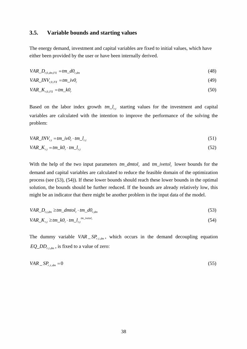
3.5. Variable bounds and starting values The energy demand, investment and capital variables are fixed to initial values, which have either been provided by the user or have been internally derived.

r,dm,dm,FXr, tm_d0VAR_D =0 (48)

rFXr, tm_iv0VAR_INV =,0 (49)

rFXr, tm_k0VAR_K =,0 (50)

Based on the labor index growth r,ttm_l starting values for the investment and capital

variables are calculated with the intention to improve the performance of the solving the problem:

r,trr,t tm_ltm_iv0VAR_INV ⋅= (51)

r,trr,t tm_ltm_k0VAR_K ⋅= (52)

With the help of the two input parameters rtm_dmtol and rtm_ivetol lower bounds for the

demand and capital variables are calculated to reduce the feasible domain of the optimization process (see (53), (54)). If these lower bounds should reach these lower bounds in the optimal solution, the bounds should be further reduced. If the bounds are already relatively low, this might be an indicator that there might be another problem in the input data of the model.

r,dmrr,t,dm tm_d0tm_dmtolVAR_D ⋅≥ (53) rtm_ivetol

r,trr,t tm_ltm_k0VAR_K ⋅≥ (54)

The dummy variable dmtrSPVAR ,,_ , which occurs in the demand decoupling equation

dmtrEQ_DD ,, , is fixed to a value of zero:

0_ ,, =dmtrSPVAR (55)

39

The two market penetration variables r,t,pVAR_XCAPP and r,t,pVAR_XCAPP1 , which are used

in the linear approximation (36) of the cost penalty term in the demand decoupling equation, are bounded by a maximum value. This maximum value corresponds to the cumulative expansion bound beyond which the cost penalty is applied.

r,pr,t,p tm_captbVAR_XCAPP ≤ (56)

r,pr,t,p tm_captbVAR_XCAPP1 ≤ (57)

40

3.6. TIMES-MACRO specific reporting parameters Several parameters are calculated for reporting purposes after each TIMES-MACRO run. Some of them are also used in the calibration routine described further below. Annual production:

r

r,c

rtm_rhorrrr 1/tm_rho

demcr,c,tr,c

tm_kpvs)tm_rho(r,t

tm_rhotm_kpvsr,trr,t LVAR_Dtm_btm_lLVAR_Ktm_aklpar_y ⎟

⎟⎠

⎞⎜⎜⎝

⎛⋅+⋅⋅= ∑

∈

⋅−⋅ .. 1

(58) Annual GDP:

trtrtr LECVARyparpar_gdp ,,, .__ −= (59)

Annual production growth rate between the periods t and t+1:

( )

⎟⎟⎟

⎠

⎞

⎜⎜⎜

⎝

⎛−⋅=

+++ 11002

1

,

1,,

1tt dd

tr

trtr par_y

par_ytm_yr (60)

Annual GDP growth rate between the periods t and t+1:

( )

⎟⎟⎟

⎠

⎞

⎜⎜⎜

⎝

⎛−⋅=

+++ 11002

1

,

1,,

1tt dd

tr

trtr par_grgdp

par_grgdppar_grgdp (61)

The marginal cost for providing the TIMES energy demand of commodity dm is calculated the following way10:

sttm_scale_crgtm_scale_n

MCOSTNRGEQMSPVAR

tm_ddf_mctr

dmtrr,t,dm ⋅−=

,

,,

._._

(62)

The reduced costs dmtrMSPVAR ,,._ describe here the change in utility, when the energy

demand is increased by one unit. The shadow price trMCOSTNRGEQ ,._ of the cost

balancing equation specifies the change in utility when the costs are changed by one unit. Hence, it can be considered as a conversion factor between utility and energy system costs (which is valid, however, only for one specific solution). The two scaling factors

rgtm_scale_n and sttm_scale_c are needed to convert the MACRO cost and energy units to

TIMES units.

10 Since the shadow price information is needed in a calibration routine of the TIMES-MACRO model (see below), which determines the so-called demand decoupling factors, the parameter name of the shadow prices for the demand commodities r,t,dmtm_ddf_mc contains the abbreviation ddf.

41

The following three calculation steps (63)-(66) are needed for the calibration routine of the TIMES-MACRO model described further below. In this calibration routine the TIMES-MACRO model is iteratively solved several times. After each model run a new labor growth rate trtm_growvn , is calculated by adjusting the previous growth rate r,ttm_growv by the

difference between the projected GDP growth rate r,ttm_gr and the actual GDP growth rate in

the model run. The projected growth rate r,ttm_gr equals the growth rate trtm_growv , initially

provided by the user. Since it is overwritten by calculation step (62), it is saved as parameter

r,ttm_gr .

r,tr,tr,ttr par_gdptm_grtm_growvtm_growvn −+=, (63)

r,TTr tm_grtm_growvn =, (64)

trtr tm_growvntm_growv ,, = (65)

The annual system costs of the middle year of the first period rtm_ec0 are also updated in the

calibration process:

sttm_scale_cT.LVAR_OBJCOStm_ec0 r,r ⋅= 0 (66)

For the calibration routine some of the results are saved in the text file ddfnew.dd, namely,

trtm_growv , , r,t,dmtm_ddf_mc , r,ttm_yr and rtm_ec0 .

42

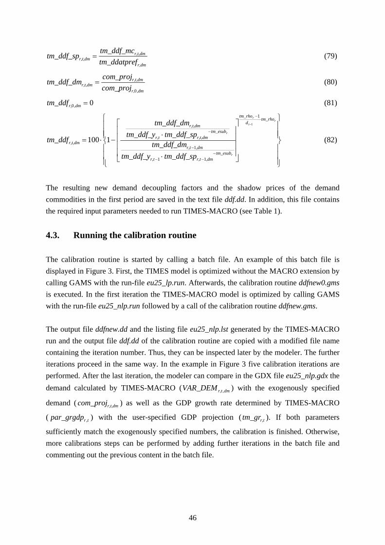
4. Calibrating a TIMES-MACRO model The purpose of the calibration is twofold: first, it should determine the so-called demand decoupling factors r,t,ctm_ddf of the demand decoupling equation (28) in such a way that the

values of the TIMES demand variables dmr,tVAR_DEM , match the exogenously specified

demand parameters r,t,dmcom_proj , secondly, the calibration routine should calculate the labor

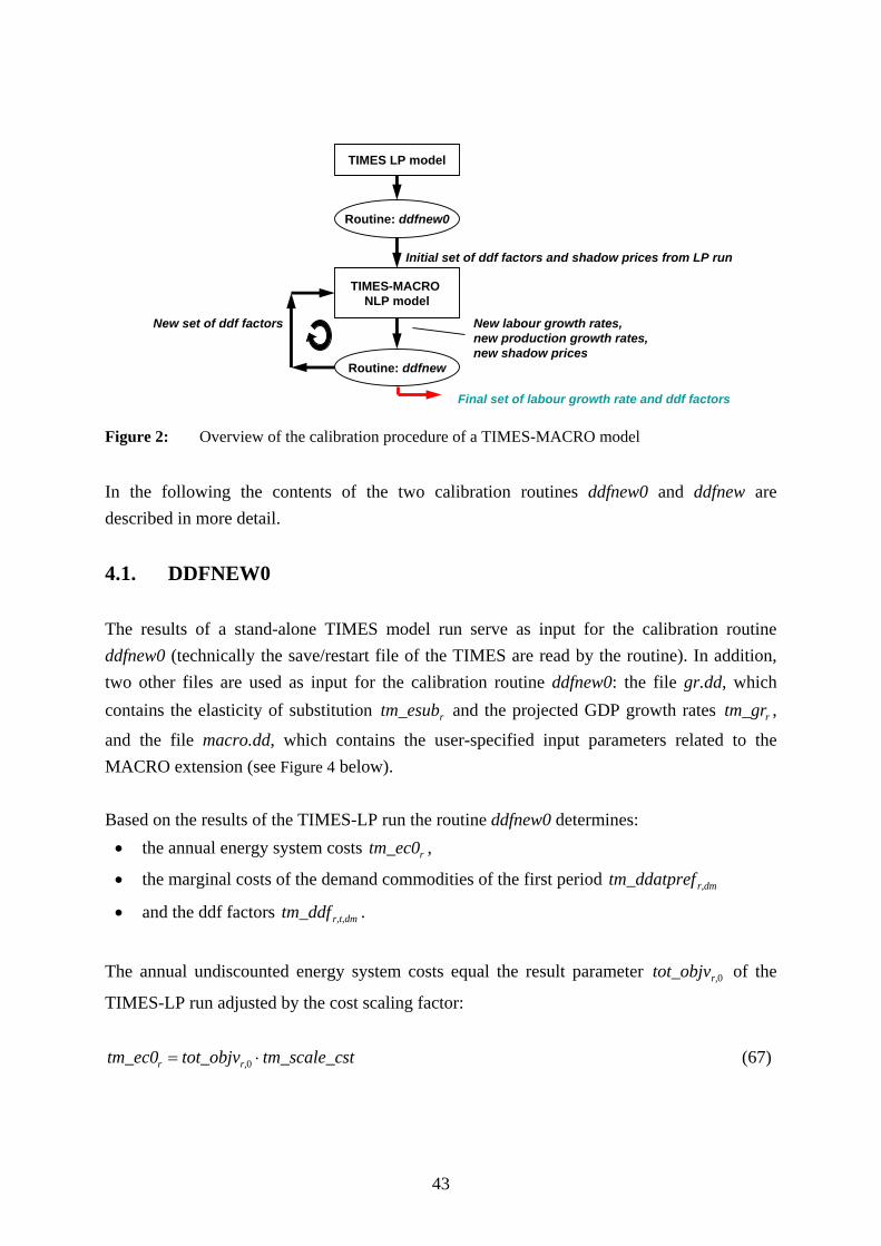
growth rates such that the user-specified GDP growth rates are matched. As a result of the calibration the results in the energy system part of the linked TIMES-MACRO model are identical to the ones when running the stand-alone TIMES model. This is not surprising since one goal of the calibration is to match the endogenous demand of the TIMES-MACRO model with the exogenous demand vector of the stand-alone TIMES model. The results of the calibrated model serve then as reference scenario to analyze the impacts, e.g. change in GDP, which are caused by adding policy constraints or measures not present in the reference scenario to the model. As mentioned already in Section 3.4.3 it is utmost important to check the behavior of the shadow prices of the demand commodities. Abrupt changes of the prices between adjacent periods should be avoided. Causes for shadow prices dropping to zero have to be eliminated before entering the calibration process, since zero values will cause a division by zero error in the course of the calibration routine. Figure 2 gives an overview of the calibration procedure. Based on the model run of a stand-alone TIMES model the calibration routine DDFNEW0 calculates an initial set of ddf factors and marginal costs for the demand commodities. With this input information the TIMES-MACRO model is run. The reporting routine after this run (see Chapter 3.6) provides new labor growth rates, new shadow prices and the production growth rates. These parameters are used in the calibration routine DDFNEW to determine a new set of ddf factors r,t,ctm_ddf .

With these new dff factors and the new labor growth rates a new TIMES-MACRO model run is started and the results are again processed in the calibration routine DDFNEW. This sequence of alternately running the TIMES-MACRO model and the calibration routine continues, until the demand calculated by TIMES-MACRO ( dmr,tVAR_DEM , ) sufficiently

matches the exogenously specified demand ( r,t,dmcom_proj ) and until the GDP growth rate

determined by TIMES-MACRO ( trpar_grgdp , ) matches the user-specified GDP projection

( r,ttm_gr ). The number of iterations in the calibration routine can be flexibly adjusted by the

modeler. For example, the modeler can specify first 5 iterations, inspect the solution and can then, if the routine has not converged yet, perform further calibration iterations in addition to the 5 already done.

43

TIMES LP model

TIMES-MACRO NLP model

Routine: ddfnew0

Routine: ddfnew

Initial set of ddf factors and shadow prices from LP run

New set of ddf factors New labour growth rates, new production growth rates,new shadow prices

Final set of labour growth rate and ddf factors

Figure 2: Overview of the calibration procedure of a TIMES-MACRO model

In the following the contents of the two calibration routines ddfnew0 and ddfnew are described in more detail.

4.1. DDFNEW0 The results of a stand-alone TIMES model run serve as input for the calibration routine ddfnew0 (technically the save/restart file of the TIMES are read by the routine). In addition, two other files are used as input for the calibration routine ddfnew0: the file gr.dd, which contains the elasticity of substitution rtm_esub and the projected GDP growth rates rtm_gr ,

and the file macro.dd, which contains the user-specified input parameters related to the MACRO extension (see Figure 4 below). Based on the results of the TIMES-LP run the routine ddfnew0 determines: • the annual energy system costs rtm_ec0 ,

• the marginal costs of the demand commodities of the first period r,dmftm_ddatpre

• and the ddf factors r,t,dmtm_ddf .

The annual undiscounted energy system costs equal the result parameter 0r,tot_objv of the

TIMES-LP run adjusted by the cost scaling factor:

sttm_scale_ctot_objvtm_ec0 r,r ⋅= 0 (67)

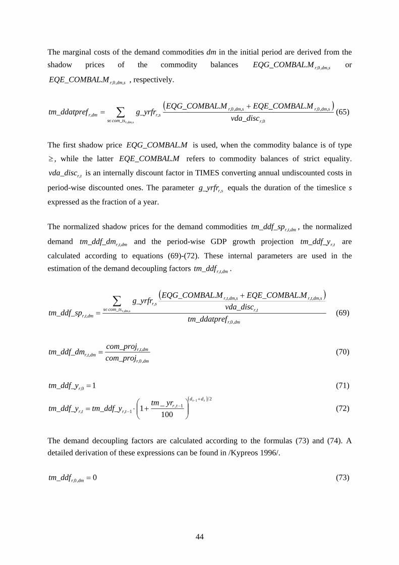
44

The marginal costs of the demand commodities dm in the initial period are derived from the shadow prices of the commodity balances ,dm,sr,MEQG_COMBAL 0. or

,dm,sr,MEQE_COMBAL 0. , respectively.

( )

∑∈

+=

r,dm,scom_tss r,

,dm,sr,,dm,sr,r,sr,dm vda_disc

MEQE_COMBALMEQG_COMBALg_yrfrftm_ddatpre

0

00 .. (65)

The first shadow price MEQG_COMBAL. is used, when the commodity balance is of type

≥ , while the latter MEQE_COMBAL. refers to commodity balances of strict equality.

r,tvda_disc is an internally discount factor in TIMES converting annual undiscounted costs in

period-wise discounted ones. The parameter r,sg_yrfr equals the duration of the timeslice s

expressed as the fraction of a year. The normalized shadow prices for the demand commodities r,t,dmtm_ddf_sp , the normalized

demand r,t,dmtm_ddf_dm and the period-wise GDP growth projection r,ttm_ddf_y are

calculated according to equations (69)-(72). These internal parameters are used in the estimation of the demand decoupling factors r,t,dmtm_ddf .

( )

,dmr,

com_tss r,t

r,t,dm,sr,t,dm,sr,s

r,t,dm ftm_ddatprevda_disc

MEQE_COMBALMEQG_COMBALg_yrfr

tm_ddf_sp r,dm,s

0

..∑∈

+

= (69)

,dmr,

r,t,dmr,t,dm com_proj

com_projtm_ddf_dm

0

= (70)

10 =r,tm_ddf_y (71)

( ) 21,

1

1

100_

1tt dd

trr,tr,t

yrtmtm_ddf_ytm_ddf_y

+−

−

−

⎟⎟⎠

⎞⎜⎜⎝

⎛+⋅= (72)

The demand decoupling factors are calculated according to the formulas (73) and (74). A detailed derivation of these expressions can be found in /Kypreos 1996/.

00 =,dmr,tm_ddf (73)

45

⎪⎪⎪

⎭

⎪⎪⎪

⎬

⎫

⎪⎪⎪

⎩

⎪⎪⎪

⎨

⎧

⎥⎥⎥⎥

⎦

⎤

⎢⎢⎢⎢

⎣

⎡

⋅

⋅−⋅=

⋅−

−−−

−

−

−r

t

r

r

r

tm_rhod

tm_rho

tm_esub,dmr,tr,t

,dmr,t

tm_esubr,t,dmr,t

r,t,dm

r,t,dm

tm_ddf_sptm_ddf_ytm_ddf_dm


tm_ddf

1

1

11

11100 (74)

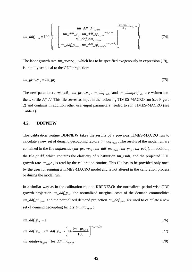
The labor growth rate r,ttm_growv , which has to be specified exogenously in expression (19),

is initially set equal to the GDP projection:

r,tr,t tm_grtm_growv = (75)

The new parameters rtm_ec0 , r,ttm_growv , r,t,dmtm_ddf and r,dmftm_ddatpre are written into

the text file ddf.dd. This file serves as input in the following TIMES-MACRO run (see Figure 2) and contains in addition other user-input parameters needed to run TIMES-MACRO (see Table 1).

4.2. DDFNEW The calibration routine DDFNEW takes the results of a previous TIMES-MACRO run to calculate a new set of demand decoupling factors r,t,dmtm_ddf . The results of the model run are

contained in the file ddfnew.dd ( trtm_growv , , r,t,dmtm_ddf_mc , r,ttm_yr , rtm_ec0 ). In addition,

the file gr.dd, which contains the elasticity of substitution rtm_esub and the projected GDP

growth rate rtm_gr , is read by the calibration routine. This file has to be provided only once

by the user for running a TIMES-MACRO model and is not altered in the calibration process or during the model run. In a similar way as in the calibration routine DDFNEW0, the normalized period-wise GDP growth projection r,ttm_ddf_y , the normalized marginal costs of the demand commodities

r,t,dmtm_ddf_sp and the normalized demand projection r,t,dmtm_ddf are used to calculate a new

set of demand decoupling factors r,t,dmtm_ddf :

10 =r,tm_ddf_y (76)

( ) 21,

1

1

100_

1tt dd

trr,tr,t

grtmtm_ddf_ytm_ddf_y

+−

−

−

⎟⎟⎠

⎞⎜⎜⎝

⎛+⋅= (77)

,dmr,r,dm tm_ddf_mcftm_ddatpre 0= (78)

46

r,dm

r,t,dmr,t,dm ftm_ddatpre

tm_ddf_mctm_ddf_sp = (79)

,dmr,

r,t,dmr,t,dm com_proj

com_projtm_ddf_dm

0

= (80)

00 =,dmr,tm_ddf (81)

⎪⎪⎪

⎭

⎪⎪⎪

⎬

⎫

⎪⎪⎪

⎩

⎪⎪⎪

⎨

⎧

⎥⎥⎥⎥

⎦

⎤

⎢⎢⎢⎢

⎣

⎡

⋅

⋅−⋅=

⋅−

−−−

−

−

−r

t

r

r

r

tm_rhod

tm_rho

tm_esub,dmr,tr,t

,dmr,t

tm_esubr,t,dmr,t

r,t,dm

r,t,dm



tm_ddf

1

1

11

11100 (82)

The resulting new demand decoupling factors and the shadow prices of the demand commodities in the first period are saved in the text file ddf.dd. In addition, this file contains the required input parameters needed to run TIMES-MACRO (see Table 1).

4.3. Running the calibration routine The calibration routine is started by calling a batch file. An example of this batch file is displayed in Figure 3. First, the TIMES model is optimized without the MACRO extension by calling GAMS with the run-file eu25_lp.run. Afterwards, the calibration routine ddfnew0.gms is executed. In the first iteration the TIMES-MACRO model is optimized by calling GAMS with the run-file eu25_nlp.run followed by a call of the calibration routine ddfnew.gms. The output file ddfnew.dd and the listing file eu25_nlp.lst generated by the TIMES-MACRO run and the output file ddf.dd of the calibration routine are copied with a modified file name containing the iteration number. Thus, they can be inspected later by the modeler. The further iterations proceed in the same way. In the example in Figure 3 five calibration iterations are performed. After the last iteration, the modeler can compare in the GDX file eu25_nlp.gdx the demand calculated by TIMES-MACRO ( dmr,tVAR_DEM , ) with the exogenously specified

demand ( r,t,dmcom_proj ) as well as the GDP growth rate determined by TIMES-MACRO

( trpar_grgdp , ) with the user-specified GDP projection ( r,ttm_gr ). If both parameters

sufficiently match the exogenously specified numbers, the calibration is finished. Otherwise, more calibrations steps can be performed by adding further iterations in the batch file and commenting out the previous content in the batch file.

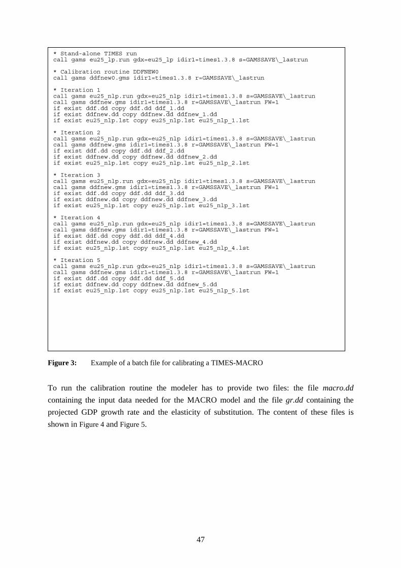
47

Figure 3: Example of a batch file for calibrating a TIMES-MACRO

To run the calibration routine the modeler has to provide two files: the file macro.dd containing the input data needed for the MACRO model and the file gr.dd containing the projected GDP growth rate and the elasticity of substitution. The content of these files is shown in Figure 4 and Figure 5.

* Stand-alone TIMES run call gams eu25_lp.run gdx=eu25_lp idir1=times1.3.8 s=GAMSSAVE\_lastrun * Calibration routine DDFNEW0 call gams ddfnew0.gms idir1=times1.3.8 r=GAMSSAVE\_lastrun * Iteration 1 call gams eu25_nlp.run gdx=eu25_nlp idir1=times1.3.8 s=GAMSSAVE\_lastrun call gams ddfnew.gms idir1=times1.3.8 r=GAMSSAVE\_lastrun FW=1 if exist ddf.dd copy ddf.dd ddf_1.dd if exist ddfnew.dd copy ddfnew.dd ddfnew_1.dd if exist eu25_nlp.lst copy eu25_nlp.lst eu25_nlp_1.lst * Iteration 2 call gams eu25_nlp.run gdx=eu25_nlp idir1=times1.3.8 s=GAMSSAVE\_lastrun call gams ddfnew.gms idir1=times1.3.8 r=GAMSSAVE\_lastrun FW=1 if exist ddf.dd copy ddf.dd ddf_2.dd if exist ddfnew.dd copy ddfnew.dd ddfnew_2.dd if exist eu25_nlp.lst copy eu25_nlp.lst eu25_nlp_2.lst * Iteration 3 call gams eu25_nlp.run gdx=eu25_nlp idir1=times1.3.8 s=GAMSSAVE\_lastrun call gams ddfnew.gms idir1=times1.3.8 r=GAMSSAVE\_lastrun FW=1 if exist ddf.dd copy ddf.dd ddf_3.dd if exist ddfnew.dd copy ddfnew.dd ddfnew_3.dd if exist eu25_nlp.lst copy eu25_nlp.lst eu25_nlp_3.lst * Iteration 4 call gams eu25_nlp.run gdx=eu25_nlp idir1=times1.3.8 s=GAMSSAVE\_lastrun call gams ddfnew.gms idir1=times1.3.8 r=GAMSSAVE\_lastrun FW=1 if exist ddf.dd copy ddf.dd ddf_4.dd if exist ddfnew.dd copy ddfnew.dd ddfnew_4.dd if exist eu25_nlp.lst copy eu25_nlp.lst eu25_nlp_4.lst * Iteration 5 call gams eu25_nlp.run gdx=eu25_nlp idir1=times1.3.8 s=GAMSSAVE\_lastrun call gams ddfnew.gms idir1=times1.3.8 r=GAMSSAVE\_lastrun FW=1 if exist ddf.dd copy ddf.dd ddf_5.dd if exist ddfnew.dd copy ddfnew.dd ddfnew_5.dd if exist eu25_nlp.lst copy eu25_nlp.lst eu25_nlp_5.lst

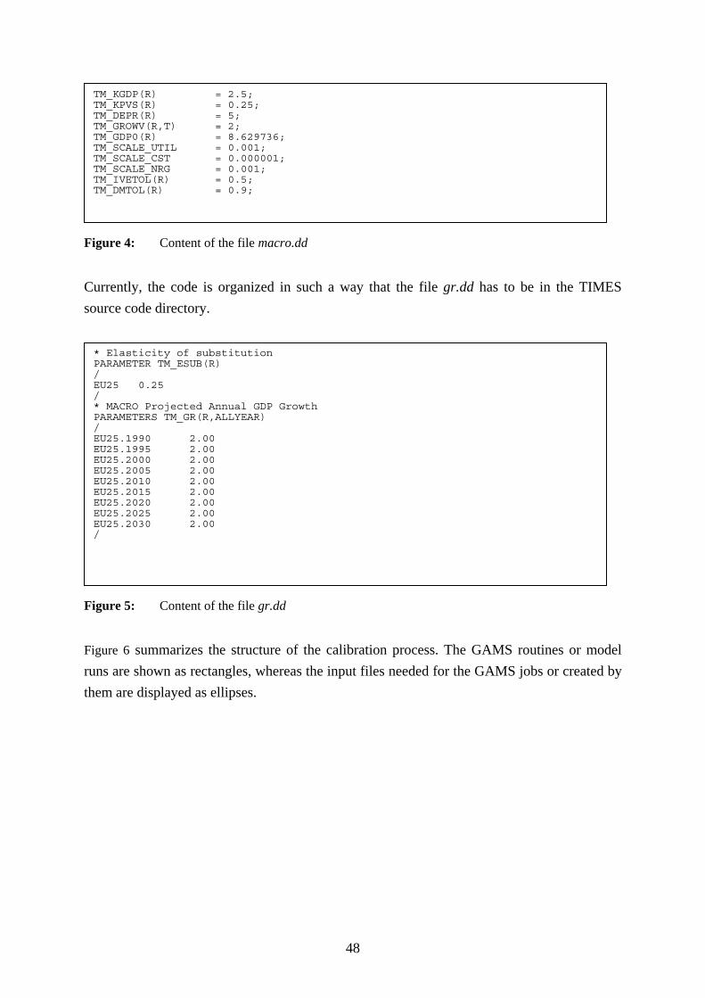
48

Figure 4: Content of the file macro.dd

Currently, the code is organized in such a way that the file gr.dd has to be in the TIMES source code directory.

Figure 5: Content of the file gr.dd

Figure 6 summarizes the structure of the calibration process. The GAMS routines or model runs are shown as rectangles, whereas the input files needed for the GAMS jobs or created by them are displayed as ellipses.

* Elasticity of substitution PARAMETER TM_ESUB(R) / EU25 0.25 / * MACRO Projected Annual GDP Growth PARAMETERS TM_GR(R,ALLYEAR) / EU25.1990 2.00 EU25.1995 2.00 EU25.2000 2.00 EU25.2005 2.00 EU25.2010 2.00 EU25.2015 2.00 EU25.2020 2.00 EU25.2025 2.00 EU25.2030 2.00 /

TM_KGDP(R) = 2.5; TM_KPVS(R) = 0.25; TM_DEPR(R) = 5; TM_GROWV(R,T) = 2; TM_GDP0(R) = 8.629736; TM_SCALE_UTIL = 0.001; TM_SCALE_CST = 0.000001; TM_SCALE_NRG = 0.001; TM_IVETOL(R) = 0.5; TM_DMTOL(R) = 0.9;

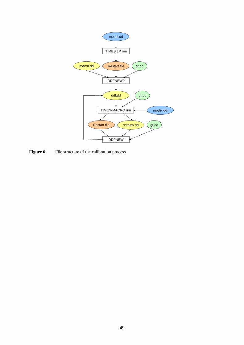
49

TIMES LP run

DDFNEW0

gr.ddmacro.dd

ddf.dd gr.dd

TIMES-MACRO run

DDFNEW

Restart file gr.dd

model.dd

Restart file

ddfnew.dd

model.dd

Figure 6: File structure of the calibration process

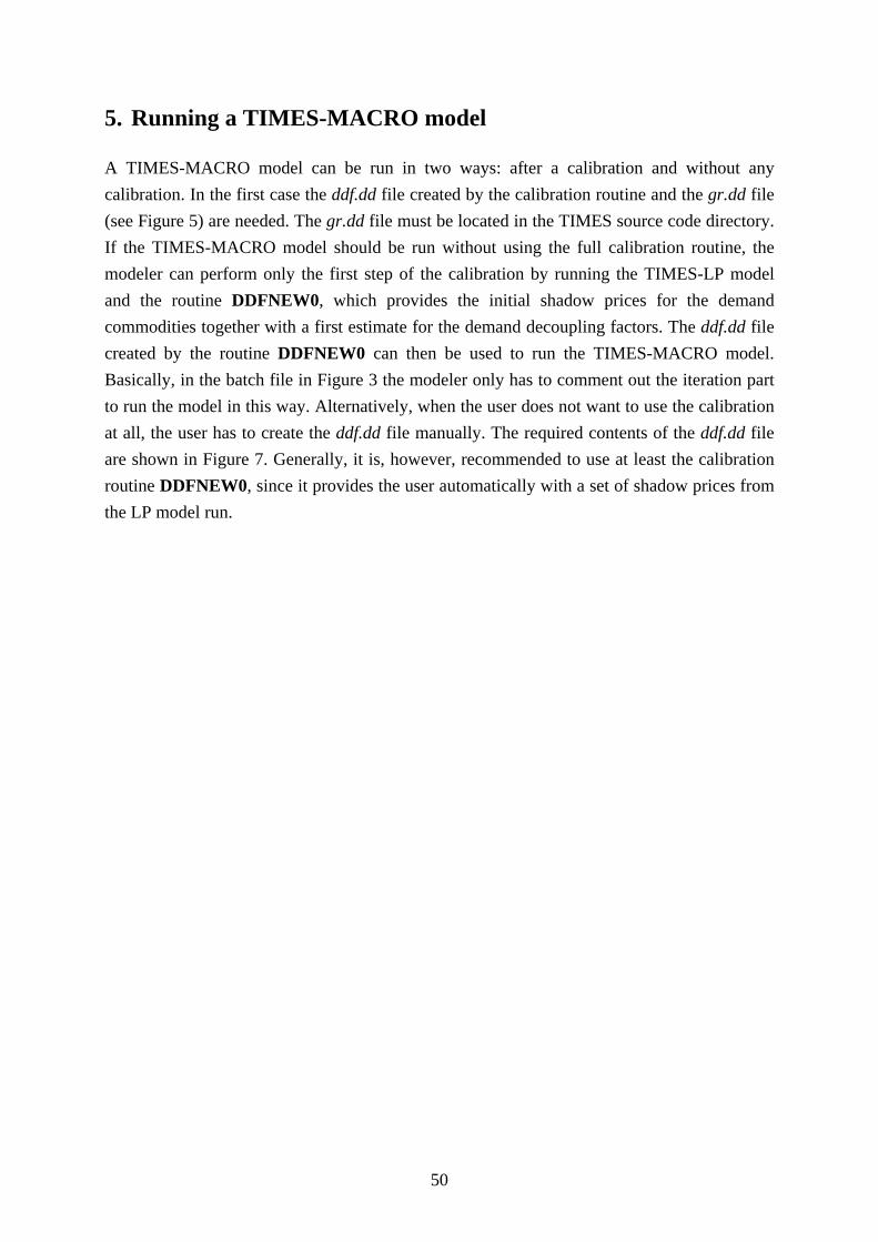
50

5. Running a TIMES-MACRO model A TIMES-MACRO model can be run in two ways: after a calibration and without any calibration. In the first case the ddf.dd file created by the calibration routine and the gr.dd file (see Figure 5) are needed. The gr.dd file must be located in the TIMES source code directory. If the TIMES-MACRO model should be run without using the full calibration routine, the modeler can perform only the first step of the calibration by running the TIMES-LP model and the routine DDFNEW0, which provides the initial shadow prices for the demand commodities together with a first estimate for the demand decoupling factors. The ddf.dd file created by the routine DDFNEW0 can then be used to run the TIMES-MACRO model. Basically, in the batch file in Figure 3 the modeler only has to comment out the iteration part to run the model in this way. Alternatively, when the user does not want to use the calibration at all, the user has to create the ddf.dd file manually. The required contents of the ddf.dd file are shown in Figure 7. Generally, it is, however, recommended to use at least the calibration routine DDFNEW0, since it provides the user automatically with a set of shadow prices from the LP model run.

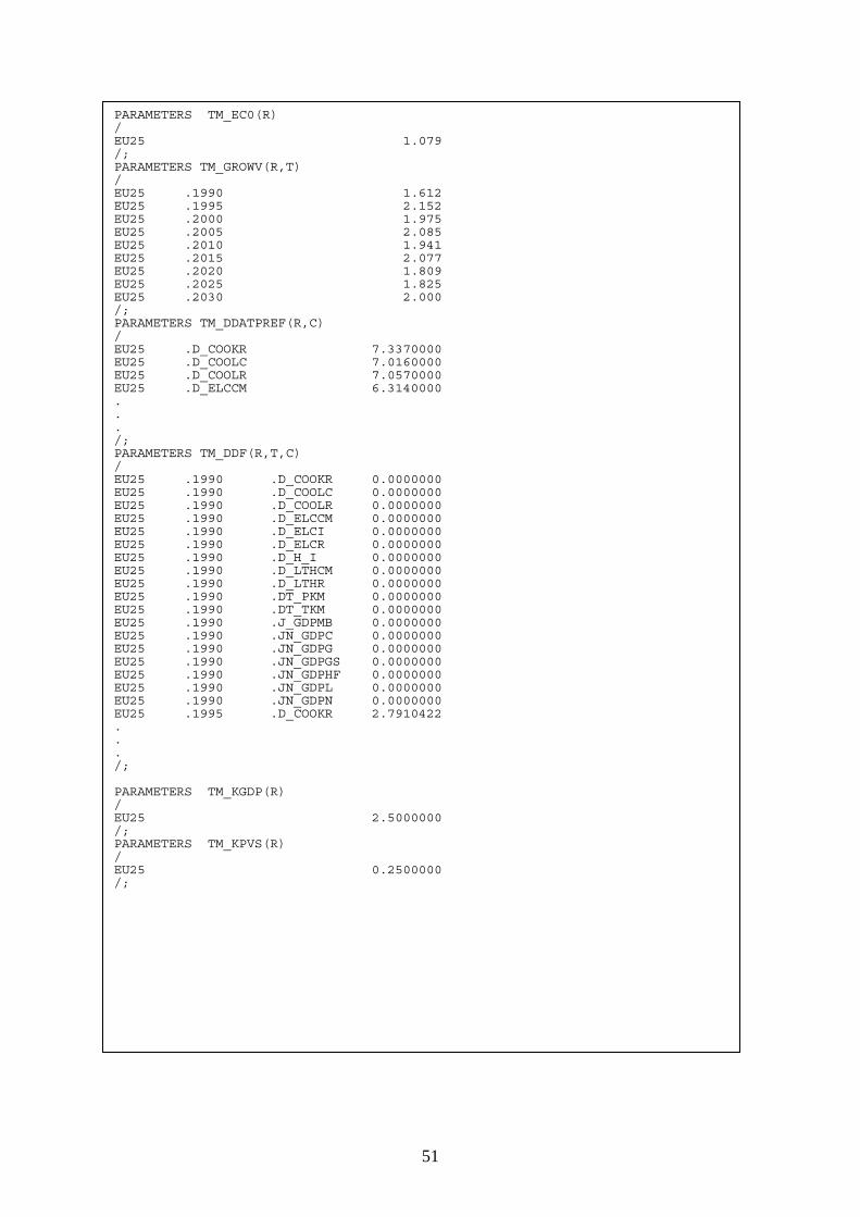
51

PARAMETERS TM_EC0(R) / EU25 1.079 /; PARAMETERS TM_GROWV(R,T) / EU25 .1990 1.612 EU25 .1995 2.152 EU25 .2000 1.975 EU25 .2005 2.085 EU25 .2010 1.941 EU25 .2015 2.077 EU25 .2020 1.809 EU25 .2025 1.825 EU25 .2030 2.000 /; PARAMETERS TM_DDATPREF(R,C) / EU25 .D_COOKR 7.3370000 EU25 .D_COOLC 7.0160000 EU25 .D_COOLR 7.0570000 EU25 .D_ELCCM 6.3140000 . . . /; PARAMETERS TM_DDF(R,T,C) / EU25 .1990 .D_COOKR 0.0000000 EU25 .1990 .D_COOLC 0.0000000 EU25 .1990 .D_COOLR 0.0000000 EU25 .1990 .D_ELCCM 0.0000000 EU25 .1990 .D_ELCI 0.0000000 EU25 .1990 .D_ELCR 0.0000000 EU25 .1990 .D_H_I 0.0000000 EU25 .1990 .D_LTHCM 0.0000000 EU25 .1990 .D_LTHR 0.0000000 EU25 .1990 .DT_PKM 0.0000000 EU25 .1990 .DT_TKM 0.0000000 EU25 .1990 .J_GDPMB 0.0000000 EU25 .1990 .JN_GDPC 0.0000000 EU25 .1990 .JN_GDPG 0.0000000 EU25 .1990 .JN_GDPGS 0.0000000 EU25 .1990 .JN_GDPHF 0.0000000 EU25 .1990 .JN_GDPL 0.0000000 EU25 .1990 .JN_GDPN 0.0000000 EU25 .1995 .D_COOKR 2.7910422 . . . /; PARAMETERS TM_KGDP(R) / EU25 2.5000000 /; PARAMETERS TM_KPVS(R) / EU25 0.2500000 /;

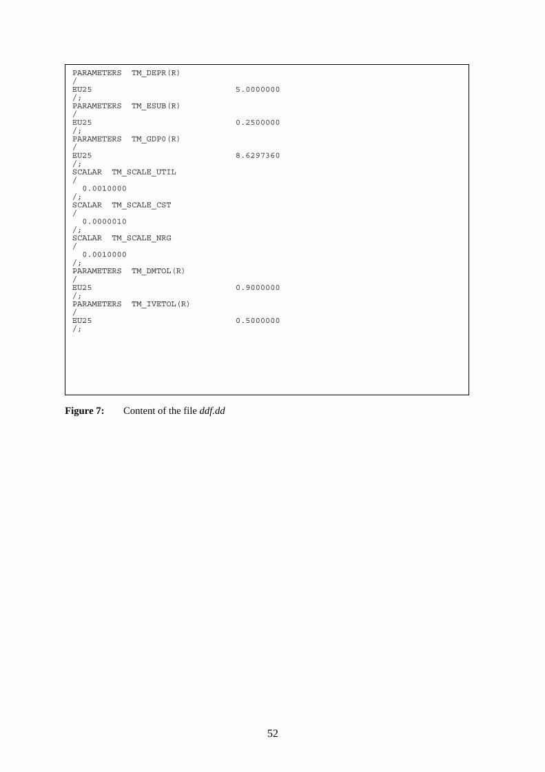
52

Figure 7: Content of the file ddf.dd

PARAMETERS TM_DEPR(R) / EU25 5.0000000 /; PARAMETERS TM_ESUB(R) / EU25 0.2500000 /; PARAMETERS TM_GDP0(R) / EU25 8.6297360 /; SCALAR TM_SCALE_UTIL / 0.0010000 /; SCALAR TM_SCALE_CST / 0.0000010 /; SCALAR TM_SCALE_NRG / 0.0010000 /; PARAMETERS TM_DMTOL(R) / EU25 0.9000000 /; PARAMETERS TM_IVETOL(R) / EU25 0.5000000 /;

53

6. Solution issues

6.1. Reduction algorithm When solving a TIMES-MACRO model it is recommended to use the internal reduction algorithm within TIMES. It reduces the number of equations and variables by various substitution and elimination steps. Since NLP solvers, as MINOS or CONOPT, in contrast do LP solvers do not contain a reduction algorithm, decreasing the model size already in TIMES helps to reduce the solution time of the NLP solver. The TIMES reduction algorithm in TIMES is activated by setting the dollar control switch REDUCE to YES in the run-file: $ SET REDUCE 'YES'

6.2. Solver One should try different NLP solvers, if available, to test which one solves the problem best. Since the only non-linear equation of the TIMES-MACRO model is the objective function, the MINOS solver, which is considered to work well with problems having few non-linear and many linear constraints, should be the first choice. One should note that two different solvers are available in MINOS: MINOS5 is the newer one, MINOS the older one. For some TIMES-MACRO models it has been observed that the older solver MINOS works better than the newer one. The solver can be set by adding the line OPTION NLP = MINOS/MINOS5/CONOPT

in the top of the run file

6.3. Starting values To reduce the solution time of NLP problems, it is usually helpful to provide starting values for the decision variables. By uncommenting the following two lines in the file solve.mod, which is found in TIMES source code directory, the results of previous model run can be used as starting values for the current run: $gdxin %RUN_NAME%.gdx $load var_act var_flo var_ncap var_ire

The name of the GDX file with the result of the previous run must equal the name contained in the dollar control parameter RUN_NAME. It is specified in the run-file.

54

Literature /Böhringer 1998/ Böhringer, C.: The Synthesis of Bottom-up and Top-down in Energy Policy modeling, Energy Economics 20 (1998), p. 233-248 /Böhringer and Rutherford 2005/ Böhringer, C., and Rutherford, T.F.: Integrating Bottom-Up into Top-Down: A Mixed Complementarity Approach, Discussion Paper No. 05-28, Centre for European Economic Research, 2005 /Büeler 1997/ Büeler, B. P.: Computing economic equilibria and its application to international trade of CO2, Dissertation ETH Zürich, 1997 /Kypreos 1996/ Kypreos, S.: The MARKAL-MACRO model and the Climate Change. Paul Scherrer Institut, Department of General Energy, PSI Bericht 96-14, Villigen/Switzerland, 1996 /Läge 2001/ Läge, E.: Entwicklung des Energiesektors im Spannungsfeld von Klimaschutz und Ökonomie: Eine modellgestützte Analyse, Dissertation, Institut für Energiewirtschaft und Rationelle Energieanwendung, Universität Stuttgart, 2001. /Loulou, et. al. 2004/ Loulou, R., Goldstein, G., Noble, K.: Documentation of the MARKAL family of models: Part II-MARKAL-MACRO, www.etsap.org, 2004 /Loulou, et. al. 2005/ Loulou, R., Remme, U., Kanudia, A., Lehtilä, A., Goldstein, G.: Documentation of the TIMES model, www.etsap.org, 2005 /Manne and Wene 1992/ Manne, A. S., and Wene, C.-O.: MARKAL-MACRO: A Linked model for Energy-Economy Analysis, Bookhaven national Laboratory, BNL-47161, 1992

Documents

Documentation of the TIMES-MACRO model - IEA-ETSAP · Energy Technology Systems Analysis Programme Documentation of the TIMES-MACRO model DRAFT Version Uwe Remme, Markus Blesl