Embed Size (px)
Citation preview
ED 418 041
AUTHOR
TITLE
INSTITUTIONISBNPUB DATENOTE
AVAILABLE FROM
PUB TYPEEDRS PRICEDESCRIPTORS
IDENTIFIERS
ABSTRACT
DOCUMENT RESUME
SO 028 730
Betts, Jeanette Gardner, Ed.; Hardwick, Susan W., Ed.;Hobbs, Gail L., Ed.Santa Barbara and California's Central Coast Region: Imagesand Encounters. A Pathways in Geography Resource PublicationNo. 15.National Council for Geographic Education.ISBN-1-884136-10-91996-00-0098p.; Prepared for the meeting of the National Council forGeographic Education (81st, Santa Barbara, CA, November13-16, 1996).National Council for Geographic Education, 16A Leonard Hall,Indiana University of Pennsylvania, Indiana, PA 15705-1087.Guides Non-Classroom (055)MF01/PC04 Plus Postage.Community; *Geographic Concepts; *Geographic Location;*Geography; *Geography Instruction; Global Education; LocalHistory; Secondary Education; Social Studies; State History*California (Central Coast Region); *California (SantaBarbara)
This annual meeting site guide is the fourth to be publishedby the National Council for Geographic Education as part of the "Pathways inGeography" series. The chapters illustrate some of the interactions betweenpeople and place that have helped shape the Santa Barbara (California) regionover the centuries. The book includes an introduction by the editors and ninechapters written by various authors. The final chapter of the book containsfive learning activities which focus on some aspect of California geography.Chapters include: (1) "Santa Barbara, California: An Unauthorized Biographyof an Image" (Thomas Herman); (2) "California Missions: The Early Years"(David Hornbeck); (3) "California Population" (William Bowen); (4) "PhysicalLandscape" (Joel Michaelsen); (5) "The San Andreas Fault" (Antony R. Orme);(6) "Santa Barbara's Water Resources" (Kate Rees, Editor); (7) "AgriculturalPatterns in Ventura County's Heartland" (Chris Mainzer); (8) "Wines of SantaBarbara County: A Geographic Perspective" (Vatche P. Tchakerian; Robert S.Bednarz); and (9) "The View from Paradise: Problems and Prospects of theCalifornia Central Coast" (William C. Halperin; Lisa Knox Burns). (EH)
********************************************************************************
Reproductions supplied by EDRS are the best that can be madefrom the original document.
********************************************************************************
NO
A PATHWAYS IN GEOGRAPHYResource Publication
The National Council forGeographic Education
U.S. DEPARTMENT OF EDUCATIONOffice of Educational Research and Improvement
EDU TIONAL RESOURCES INFORMATIONCENTER (ERIC)
This document has been reproduced asreceived from the person or organizationoriginating it
Minor changes have been made toimprove reproduction quality
PERMISSION TO REPRODUCE ANDDISSEMINATE THIS MATERIAL HAS
BEEN GRANTED BY
TO THE EDUCATIONAL RESOURCESPoints of view or opinions stated in this INFORMATION CENTER (ERIC)document do not necessarily representofficial OERI position or policy.
Santa Barbaraand California'sCentral CoastRegion:Images and Encounters
Jeanette Gardner Betts, Susan W.Hardwick and Gail L. Hobbs,Editors
Prepared for the 81st meeting of the NationalCouncil for Geographic Education, Santa Barbara,California, November 13- 16,1996
4BEST COPY AVAILABLE
Titles in the PATHWAYS IN GEOGRAPHY Series1. Gersmehl, Philip J. 1991. Revised 1996. The Language of Maps.2. Andrews, Sona Karentz, Amy Otis-Wilbom, and Trinka Messenheimer-Young.
1991. Beyond Seeing and Hearing: Teaching Geography to Sensory ImpairedChildren - An Integrated Based Curriculum Approach.
3. Waterstone, Marvin. 1992. Water in the Global Environment.4. Martinson, Tom L. and Susan R. Brooker-Gross, eds. 1992. Revisiting the
Americas: Teaching and Learning the Geography of the Western Hemisphere.5. LeVasseur, Michal. 1993. Finding a Way: Encouraging Underrepresented
Groups in Geography = An Annotated Bibliography.6. Ennals, Peter. 1993. The Canadian Maritimes: Images and Encounters.7. Slater, Frances. 1993. Learning through Geography.8. Baumann, Paul R. 1994. Up Close from Afar: Using Remote Sensing to Teach the
American Landscape.9. Benhart, John E. and Alex Margin. 1994. Wetlands: Science, Politics, and
Geographical Relationships.10. Ulack, Richard, Karl B. Raitz, and Hilary Lambert Hopper, eds. 1994. Lexington
and Kentucky's Inner Bluegrass Region.11. Forsyth, Alfred S., Jr. 1995. Learning Geography: An Annotated Bibliography
of Research Paths.12. Petersen, James F. and Julie Mason, eds. 1995. A Geographic Glimpse of Central
Texas and the Borderlands: Images and Encounters.13. Castner, Henry W. 1995. Discerning New Horizons: A Perceptual Approach
to Geographic Education.14. Thomas, James W. 1996. A Teacher's Index to FOCUS, 1950-1993.15. Betts, Jeanette Gardner, Susan W. Hardwick, and Gail L. Hobbs, eds. 1996. Santa
Barbara and California's Central Coast Region: Images and Encounters.
Special Publications Advisory BoardSalvatore J. Natoli, Editor of Special Publications, Washington, DC
Janice Monk, University of Arizona
Eugene J. Kinemey, University of the District of Columbia
Alice Andrews, George Mason University
National Council for Geographic Education Officers 1996James Marran, President, Wilmette, IL
Edward A. Femald, Past President, Florida State University
David A. Lanegran, Vice President, Curriculum and Instruction, Macalester College, MN
Gail Hobbs, Vice President, Curriculum and Instruction, Pierce College, CA
Donald Zeigler, Vice President, Research and External Relations. Old Dominion Univ.
Martha B. Sharma, Vice President, Publications and Products, National Cathedral School
Celeste J. Fraser, Vice President, Finance, Wilhnette, IL
Sandra Pritchard, Recording Secretary, West Chester University, PA
Ruth I. Shirey, Executive Director, Indiana University of Pennsylvania
National Council for Geographic Education16A Leonard Hall
Indiana University of PennsylvaniaIndiana, Pennsylvania 15705
© 1996
A PATHWAYS IN GEOGRAPHYResource Publication
The National Council forGeographic Education
The PATHWAYS IN GEOGRAPHY series hasbeen created by the Special PublicationsAdvisory Board of the National Council forGeographic Education to support theteaching and learning of themes, conceptsand skills in geography at all levels ofinstruction.
Santa Barbaraand California'sCentral CoastRegion:Images and Encounters
Jeanette Gardner Betts, Susan W.Hardwick and Gail L. Hobbs,Editors
Prepared for the 81st meeting of the NationalCouncil for Geographic Education, Santa Barbara,California, November 13- 16,1996
PATHWAYS IN GEOGRAPHY Series Title No. 15
Santa Barbara and California's Central Coast Region: Images and Encounters
Jeanette Gardner Betts, Susan W Hardwick and Gail L. Hobbs, Editors
Copyright © 1996 by the National Council for Geographic Education.All rights reserved.
No part of this book may be reproduced or transmitted in any form or by any means, electronic or mechani-cal, including photocopying, recording, or by any information storage and retrieval system, without writtenpermission from the publisher.Materials may be copied by educators for classroom use only without obtaining permission.
For information about this title or about the series:National Council for Geographic Education16A Leonard Hall, Indiana University of PennsylvaniaIndiana, PA 15705
ISBN 1-884136-10-9
Printed in the United States of America.
ii
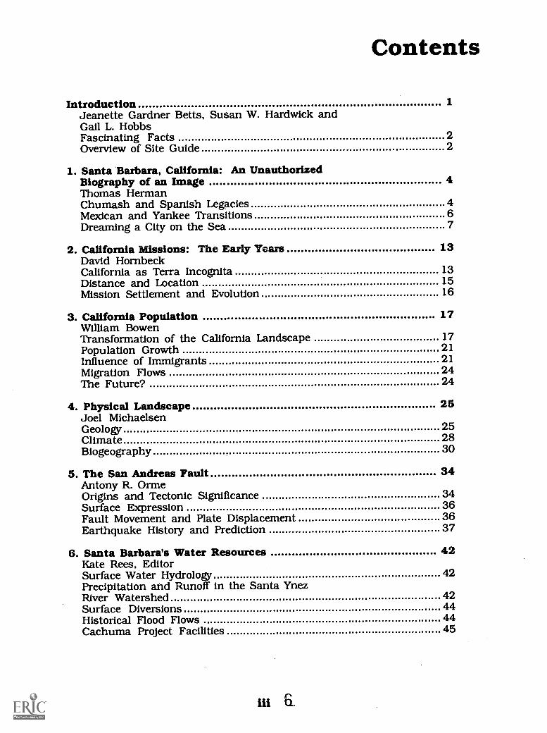
Contents
Introduction 1Jeanette Gardner Betts, Susan W. Hardwick andGail L. HobbsFascinating Facts 2Overview of Site Guide 2
1. Santa Barbara, California: An UnauthorizedBiography of an Image 4Thomas HermanChumash and Spanish Legacies 4Mexican and Yankee Transitions 6Dreaming a City on the Sea 7
2. California Missions: The Early Years 13David HornbeckCalifornia as Terra Incognita 13Distance and Location 15Mission Settlement and Evolution 16
3. California Population 17William BowenTransformation of the California Landscape 17Population Growth 21Influence of Immigrants 21Migration Flows 24The Future? 24
4. Physical Landscape 25Joel MichaelsenGeology 25Climate 28Biogeography 30
5. The San Andreas Fault 34Antony R. OrmeOrigins and Tectonic Significance 34Surface Expression 36Fault Movement and Plate Displacement 36Earthquake History and Prediction 37
6. Santa Barbara's Water Resources 42Kate Rees, EditorSurface Water Hydrology 42Precipitation and Runoff in the Santa YnezRiver Watershed 42Surface Diversions 44Historical Flood Flows 44Cachuma Project Facilities 45
in a
Bradbury Dam and Lake Cachuma ........... ......... ...... ................... 45Conveyance Facilites 45Groundwater Resources: South Coast Basins 45Groundwater Resources: Downstream Basins 46Groundwater Resources: Santa Ynez RiverRiparian Basin 46Groundwater Resources: Santa Ynez Uplandsand Buellton Basins 47Groundwater Resources: Lompoc Basin 47
7. Agricultural Patterns in Ventura County'sHeartland 49Chris MainzerArable Land 49Water 49Agricultural Connections 51
8. Wines of Santa Barbara County: A GeographicPerspective 52Vatche P. Tchakerian and Robert S. BednarzHistorical Background 52Physical Geography 52Wines and Wineries 54
9. The View from Paradise: Problems and Prospectsof the California Central CoastWilliam C. Halperin and Lisa Knox BurnsSummary of Geographical PhenomenaEconomics of the AreaRegional Growth ForecastPreserving the Quality of. Life
10. Learning ActivitesLesson Plan A. Weather or Not: Making and Usinga ClimographJerry R. and Terry WilliamsLesson Plan B. California's Mountain LionsJerry R. and Terry WilliamsLession Plan C. Water and the CaliforniaLandscape: A Geographical Perspective 69Jerry R. and Terry WilliamsLesson Plan D. The Travels of a Monarch 74Carol DouglassLesson Plan E. Rice: A World Food 78Eunice Gavin
55
55555657
58
58
65
iv
IllustrationsFigures
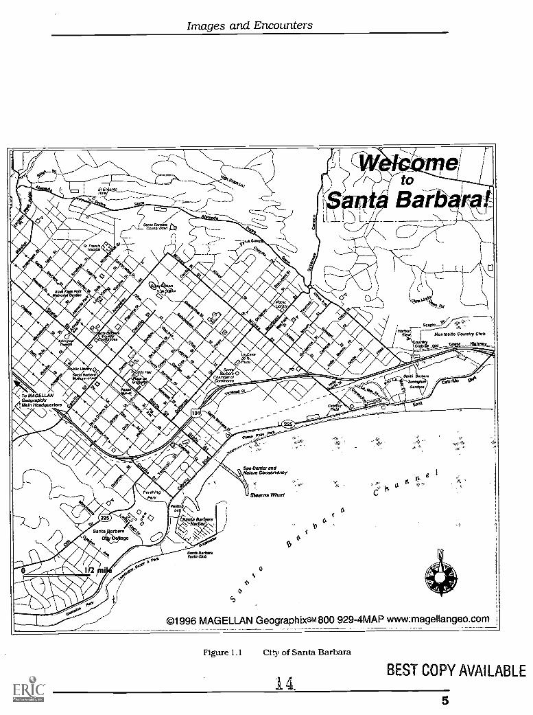
1.1City of Santa Barbara(Welcome to Santa Barbara!)
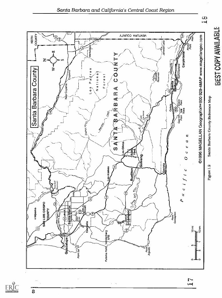
1.2Santa Barbara County Reference Map
2.1California Missions
3.1California Population, 1995
3.2United States County Population, 1995
3.3Estimated Population Change, 1990-2000
3.4Foreign-born in Metropolitan Los AngelesCounty (Frequency) 22
3.5Foreign-born in Metropolitan Los AngelesCounty (Percent) 22
3.6Estimated Percentage Population Change,1990-2000 23
4.1Santa Barbara County PhysicalFeatures 26
5.1San Andreas Fault System, Other QuaternaryFaults, and Historic Earthquakes in California 35
6.1Santa Ynez River Watershed 43
7.1Ventura County Agriculture 50
8.1Santa Barbara County Wineries 53
9.1Employment by Sector, Santa BarbaraCounty 56
5
8
14
18
19
20
Tables
7.1Ventura1993
7.2VenturaCrops
County: Ten Leading Crops
County: Other Million Dollar
v
50
50
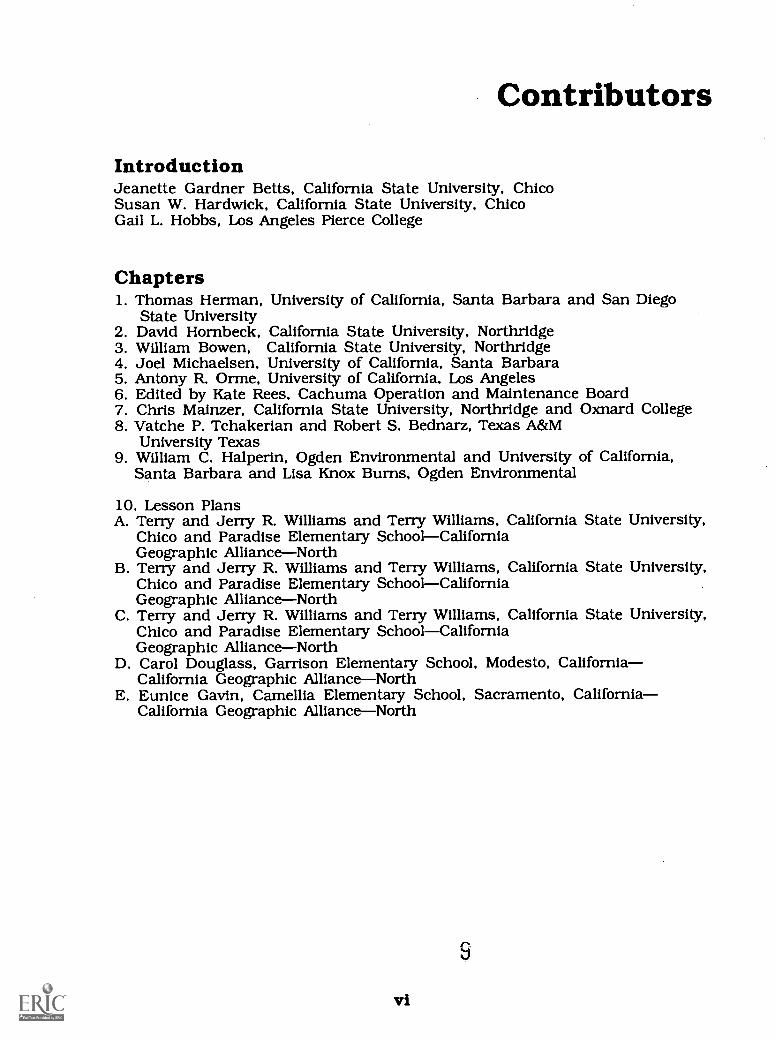
Contributors
IntroductionJeanette Gardner Betts, California State University, ChicoSusan W. Hardwick, California State University, ChicoGail L. Hobbs, Los Angeles Pierce College
Chapters1. Thomas Herman, University of California, Santa Barbara and San Diego
State University2. David Hornbeck, California State University, Northridge3. William Bowen, California State University, Northridge4. Joel Michaelsen, University of California, Santa Barbara5. Antony R. Orme, University of California, Los Angeles6. Edited by Kate Rees, Cachuma Operation and Maintenance Board7. Chris Mainzer, California State University, Northridge and Oxnard College8. Vatche P. Tchakerian and Robert S. Bednarz, Texas A&M
University Texas9. William C. Halperin, Ogden Environmental and University of California,
Santa Barbara and Lisa Knox Burns, Ogden Environmental
10. Lesson PlansA. Terry and Jerry R. Williams and Terry Williams, California State University,
Chico and Paradise Elementary SchoolCaliforniaGeographic AllianceNorth
B. Terry and Jerry R. Williams and Terry Williams, California State University,Chico and Paradise Elementary SchoolCaliforniaGeographic AllianceNorth
C. Terry and Jerry R. Williams and Terry Williams, California State University,Chico and Paradise Elementary SchoolCaliforniaGeographic AllianceNorth
D. Carol Douglass, Garrison Elementary School, Modesto, CaliforniaCalifornia Geographic AllianceNorth
E. Eunice Gavin, Camellia Elementary School, Sacramento, CaliforniaCalifornia Geographic AllianceNorth
9
vi
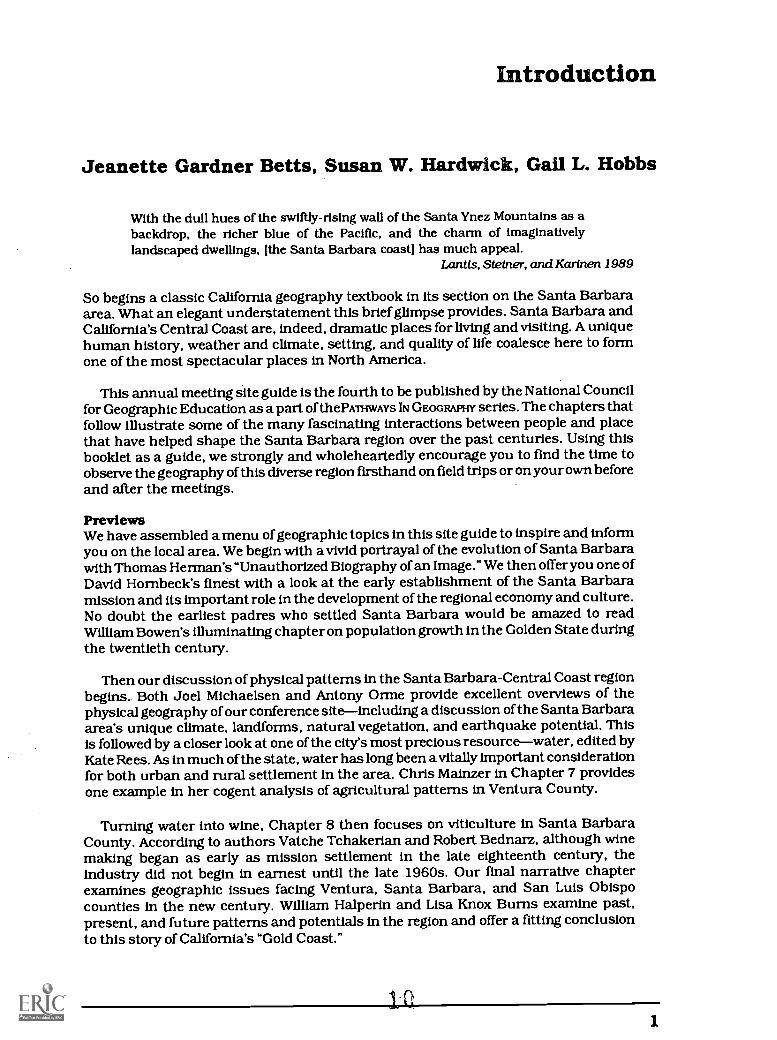
Introduction
Jeanette Gardner Betts, Susan W. Hardwick, Gail L. Hobbs
With the dull hues of the swiftly-rising wall of the Santa Ynez Mountains as abackdrop, the richer blue of the Pacific, and the charm of imaginativelylandscaped dwellings, [the Santa Barbara coast] has much appeal.
Lantis, Steiner, and Karinen 1989
So begins a classic California geography textbook in its section on the Santa Barbaraarea. What an elegant understatement this brief glimpse provides. Santa Barbara andCalifornia's Central Coast are, indeed, dramatic places for living and visiting. A uniquehuman history, weather and climate, setting, and quality of life coalesce here to formone of the most spectacular places in North America.
This annual meeting site guide is the fourth to be published by the National Councilfor Geographic Education as a part of thePAmwAys IN GEOGRAPHY series. The chapters thatfollow illustrate some of the many fascinating interactions between people and placethat have helped shape the Santa Barbara region over the past centuries. Using thisbooklet as a guide, we strongly and wholeheartedly encourage you to find the time toobserve the geography of this diverse region firsthand on field trips or on your own beforeand after the meetings.
PreviewsWe have assembled a menu of geographic topics in this site guide to inspire and informyou on the local area. We begin with a vivid portrayal of the evolution of Santa Barbarawith Thomas Herman's "Unauthorized Biography of an Image." We then offer you one ofDavid Hornbeck's finest with a look at the early establishment of the Santa Barbaramission and its important role in the development of the regional economy and culture.No doubt the earliest padres who settled Santa Barbara would be amazed to readWilliam Bowen's illuminating chapter on population growth in the Golden State duringthe twentieth century.
Then our discussion of physical patterns in the Santa Barbara-Central Coast regionbegins. Both Joel Michaelsen and Antony Orme provide excellent overviews of thephysical geography of our conference siteincluding a discussion of the Santa Barbaraarea's unique climate, landforms, natural vegetation, and earthquake potential. Thisis followed by a closer look at one of the city's most precious resourcewater, edited byKate Rees. As in much of the state, water has long been a vitally important considerationfor both urban and rural settlement in the area. Chris Mainzer in Chapter 7 providesone example in her cogent analysis of agricultural patterns in Ventura County.
Turning water into wine, Chapter 8 then focuses on viticulture in Santa BarbaraCounty. According to authors Vatche Tchakerian and Robert Bednarz, although winemaking began as early as mission settlement in the late eighteenth century, theindustry did not begin in earnest until the late 1960s. Our final narrative chapterexamines geographic issues facing Ventura, Santa Barbara, and San Luis Obispocounties in the new century. William Halperin and Lisa Knox Burns examine past,present, and future patterns and potentials in the region and offer a fitting conclusionto this story of California's "Gold Coast."
101
Santa Barbara and California's Central Coast Region
California Geographic AllianceNorth teachers Terry Williams and JerryR Williams, CarolDouglass, and Eunice Gavin present us with a collection of learning activities on thegeography of California. Their motivating and instructional examples expand not only ourknowledge, skills, and pedagogy for learning and teaching about pressing geographic issuesin the state but also offer inspiration for the creation of original activities foruse in your ownclasses when you return home.
Fascinating FactsWe offer the following tantalizing previews of the chapters that follow:
Santa Barbara was first popularized to the nation in a pamphletpublished in 1878 designed to attract health seekers. It described the smallvillage as the "sanitarium of the Pacific Coast."
A major earthquake in June 1925 leveled almost the entire city of SantaBarbara.
Cities such as Santa Barbara as Spanish missions now contain morethan 60 percent of California's population.
The Seaside Banana Gardens, located ten miles northwest on the coastfrom Ventura, raises more than 50 varieties of bananas.
Ventura County's Port Hueneme currently ships more than 200,000 tonsof citrus annually to the Pacific Rim. Its refrigerated warehouse is thelargest port facility of this kind in the Western Hemisphere.
The Santa Barbara area is home to more than 30 wineries, seventy -fivepercent of which were built after 1982.
The federal government awarded its first lease for drilling offshore oil inthe Santa Barbara Channel in 1966. Three years later, an underwater welloff the Carpinteria coast blew, spewing thousands of gallons of petroleuminto the ocean, killing wildlife and coating beaches from Ventura to SantaBarbara. This event helped launch the nation's environmental movement.
Santa Barbara AttractionsWe encourage you to visit some of the following places while you are in the area (seeFigure 1.1):
Botanical Garden-1212 Mission Canyon Road, tel. 682-4726. Thisbeautiful 65-acre preserve specializes in plants native to California.
Santa Barbara Museum of Natural History-2559 Puesta del Sol Road,tel. 682-4711. This collection of visual and textual information on thebiogeography, geomorphology, migration and settlement, and urbanevolution of the area provides useful background for your field observations.
Mission Santa Barbaracorner of East Los Olivos and Laguna streets,tel. 682-4149. Called "Queen of the Missions," this stunning building,constructed in 1786, is one of the best preserved of the missions inCalifornia.
Stearns Wharfon the water at the foot of State Street and CabrilloBoulevard. Built in 1872, this was a landmark for Santa Barbara. It was usedas a port for cargo and passenger ships and, in the 1930s, as a departurepoint for floating casino gamblers.
Alameda Plazabounded by Micheltorena, Sola, Anacapa, and Gardenstreets downtown. This is a biogeographer's paradise with more than 70varieties of trees.
Historic adobes. The city's heritage is evident in its colorful culturallandscape of white-washed, tile-roofed buildings and Spanish street names.For a sampling of Santa Barbara's New England and Latino heritage, driveby the Trussell-Winchester Adobe, built in 1854 414 West Montecito Street.You may also wish to visit Spanish-inspired Casa de la Guerra, built in1828-15 East de la Guerra Street; Casa Covarrubias, built in 1817-715Santa Barbara Street; and Hill-Carrillo Adobe, built earlier in the city'shistory in 1826-11-15 East Carillo Street.
112
Images and Encounters
One Final ExhortationWe hope the chapters that follow provide you with ample motivation and information tolaunch into the field on your own while you are in the area. A lush environment awaitsyou .We encourage you to avoid pressures from family and friends to visit only Disneylandand Knott's Berry Farm (instead of exploring the local area) in an effort to provide you withglimpses of the real (rather than the surreal) California. (That is why we have chosen SantaBarbara as the site for these California meetings!) Please, don't forget your camera.
Reference
Lantis, David W., Rodney Steiner, and Arthur E. Karinen 1989. California: Land ofContrasts. rev. ed. Dubuque, Ia.: Kendall Hunt.
12
3
1
Santa Barbara, California:An Unauthorized Biography of an ImageThomas Herman
Turn to the pages marked California in your road atlas and the city of Santa Barbara is notlikely to jump out at you as one of the more significant places in the state (Figure 1.1). Itmerely takes its place with a large collection of moderately-sized coastal cities that offer agreat deal more to residents and vacationers than they do to industry. Not only is the SantaBarbara area unique because of the local geography of an east-west running coastline andthe coastal ranges (hence the regional label "South Coast") but it is also often of marginalinterest on road atlas map pages and mental images because it is in the borderlandsbetween those two squabbling siblings, Northern and Southern California. To the moreanalytically minded, nevertheless, it may seem no more important to write the biographyof Santa Barbara than say Ventura, or maybe Manhattan Beach. It is not a major factorin the material flows that constitute the bulk of the state's economy, nor a dynamic locationto observe the changing demographics of the state's population.
Another argument, however, can be made in defense of an analysis of Santa Barbara.Aligned with this position would be the city's historical significance as a village site of theChumash and other tribes, a mission territory under Spanish rule, and a part of theterritory surrendered by Mexico to the United States in 1848. We can offer additionalsupport derived from the beauty and bounty of the natural landscape, including theprotected channel waters, enriched by the convergence of warm and cold ocean currentsoff Point Conception (to the west). The plot that also makes this biography compelling is thecontinuous interplay between Santa Barbara's aesthetic virtues and envisioning itshistory. From the time of its earliest settlers, we can attribute a special value to the areathat has in turn engendered careful treatment and ambitious designs. The result is a richand intriguing landscape that expresses historically and culturally dynamicinterpretations of and relationship to the natural landscape. These processes have turnedSanta Barbara from an important site in historical narratives to a symbol of the idealSouthern California quality and style of life. It is a city in which its citizens have given highpriority to image and architecture in a conscious effort to manage and even augmentsubstantial cultural capital. The length of this paper necessitates subordinating muchdetail while highlighting the continuity of this aesthetic theme and suggesting how historyhas been reappropriated and reintegrated into the Santa Barbara landscape to maintainselective connections with the events and cultures of the past.
Chumash and Spanish LegaciesIn October of 1542, Juan Rodriguez Cabrillo led the first European expedition into thisregion. Though he was Portuguese, his two ships sailed under the flag of Spain. Theyentered what is now the Santa Barbara Channel to anchor in the lee of the channel islandsand were welcomed by canoes full of the local inhabitants, the Chumash, called theCanalirlos by the Spanish. Mixing with other hunting peoples in the area as early as A.D.800, they had evolved a culture reminiscent of Polynesia. They lived together in communallong houses and fed themselves from the ample supply of sea life. They navigated the watersof the channel in canoes of up to 25 feet (7.6 m), carved from fallen redwoods that had drifteddown the coast with the currents and washed ashore in the local eddy. At night, they usedbeacon fires atop the coastal heights for reference. The life the Chumash led reflected anotably higher level of advancement and quality of life than other Native Americans of theregion. To European explorers, the Canalirlos became an asset because of their friendlinessand abilities.
4
Images artd Encounters
To MAGELLANGeographixMain Headquarters
©1996 MAGELLAN Geographixsm 800 929-4MAP www:magellangeo.com
Figure 1.1 City of Santa Barbara
14.BEST COPY AVAILABLE
Santa Barbara and California's Central Coast RegionFor more than 200 years the Spanish made only temporary visits. In 1602, Sebastian
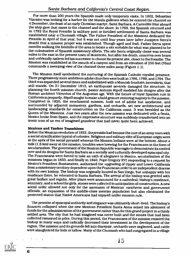
Vizcaino was looking for a harbor for the Manila galleons when he entered the channel on4 December, the feast of an early Christian martyr, Saint Barbara. A Carmelite friar aboardthe ship gave that name to the channel and the shore. In 1769, the Spanish returned andin 1782 the Royal Presidio (a military post or fortified settlement) of Santa Barbara wasestablished near a Chumash village. The Father President of the Missions dedicated thePresidio in April of that year, but it was not until four years later (after Junipero Serra'sdeath) that a mission proper was established. Though aged and frail, Father Serra spentmonths walking the foothills of the area to locate a site suitable for what was planned to bethe culmination of Spanish missionary efforts. The site Serra originally chose was severalmiles to the east in the present town of Montecito, but after his death, concerns over bearsand unfriendly natives led his successor to choose its present site, closer to the Presidio. TheMission was established at the mouth of a canyon and from an elevation of 250 feet (76m)commands a sweeping view of the channel three miles away (Figure 1.1).
The Mission itself symbolized the nurturing of the Spanish Catholic royalist presence.Three progressively more ambitious adobe churches were built in 1786, 1789, and 1794. Thethird was expanded several times and embellished with a Moorish fountain, lavendaria, thatstill stands. On 21 December 1812, an earthquake severely damaged the structure. Inplanning the fourth mission church, pastor Antonio Ripoll modeled his designs after theRoman architect Vitruvius of the Augustan age. With the future of royal Spanish rule inCalifornia in jeopardy, Ripoll sought to make a bold gesture restoring majesty to the mission.Completed in 1820, the neoclassical mission, built not of adobe but sandstone, andsurrounded by adjacent monastery, gardens, and orchards, set new architectural andlandscaping standards for construction on the California coast. It was heralded as theQueen of the Missions. Just two years after the new mission was dedicated with a fiesta.Mexico broke from Spain, and the impressive structure was suddenly transformed into anironic icon of an era of imagined grandeur that had never quite been achieved.
Mexican and Yankee TransitionsBefore the Mexican revolution of 1822, thepresidio had become the core of an army town witha social stratification typical of colonies. Religious and military elite of European origin wereat the apex of the social pyramid whereas the Mission Indians were at the bottom. About amile (1.6 km) away at the mission, troubles were brewing for the Franciscans in the form ofsecularization. The government of the Mexican Republic was eager to demonstrate its controlover and its designs for Santa Barbara as a socially and culturally developed episcopal city.The Franciscans were forced to take an oath of allegiance to Mexico, secularization of themissions began in 1833, and finally in 1840, Pope Gregory XVI responding to a request byMexico's President Bustamente, authorized the upgrading of Upper and Lower Californiafrom a missionary territory dependent upon the Franciscan order to an independent diocesewith its own bishop. The bishop was originally located in San Diego, but unhappy with hisresidence there, he relocated to Santa Barbara. The arrival of the bishop was greeted withgreat fanfare and regalia. After plans were announced for a cathedral, bishop's residence,seminary, and a school for girls, stones were collected in anticipation of construction. A newsocial order allowed not only for the ascension of Mexican rancheros and governmentofficials, an expansion of the middle-class mestizo population but also eliminated theprotected status that Native Americans had enjoyed under mission rule.
The promise of episcopal authority and elegance was ultimately short-lived. The bishop'sfinances collapsed when the new Mexican President Santa Anna seized his allotment offunds for the administration of the government rather than for this grand project in a thinlysettled area. The city that he had imagined was never built and the stones that had beencollected remained in piles. During this period, the Franciscans of the mission resisted thebishop in many ways and radically decreased their investment in the development of theregion. The mission and its grounds fell into disrepair, orchards were neglected, and cattlewere slaughtered for hide or tallow. Many of the Chumash who had congregated in a village
15
6
Images and Encounters
of adobe huts around the mission began to resume their roving ways, and social problemsflourished. For a time, before the United States government took over California, the missionchurch was rented to Goleta Valley ranchers. Though this was a tumultuous andunproductive period for the development of Santa Barbara, the visions of Bishop GarciaDiego y Moreno of Santa Barbara as a northern outpost of Hispanic civilization spurred theimaginations of future residents and boosters. If only for four short years, the city had takenits place as the religious and cultural capital of California.
During the Mexican period, the military officials of the garrison at Santa Barbara werealso prominent traders. None more so than Captain De La Guerra, who was commandanteunder both Spanish and Mexican rule before retiring from active military service. He builta large adobe that became the center of social life for the town. De La Guerra had establishedcontacts with several American traders and investors, some of whom migrated to California,became Hispanicized, and married daughters of De La Guerra. Two Americans who spentperiods in Santa Barbara, Alfred Robinson and Richard Henry Dana, Jr., each wrote booksthat made Americans aware of the character of Hispanic California. Robinson in particularconveyed an empathy for the Hispanic culture and through his accounts developed anarchetype of the lifestyle of the region.
Yankee appreciation, or more accurately accommodation, of Hispanic culture helpedcontribute to amicable relations from the time of occupation in 1846 through the 1860s,when the Spanish-surnamed Barbareftos comprised 70 percent of the city's 2,500population. Hispanic leaders represented the city and county in public office and served inthe Union army during the Civil War. Even the street names, adopted after the 1851 surveyof the city, faithfully recalled the cultures of the past, including Chumash chiefs' names,families of the Spanish and Mexican eras, names from the recent American experience, andSpanish topographical destinations to fill out the map. A drought struck in 1863-64 andweakened the cattle economy. After that, a trend developed of Hispanic land owners losingtheir holdings to Anglos, and this triggered a widespread migration of the Hispanic andmestizo artisan class. By the 1870s, Hispanics played only a minor role in the import andmerchandising sector, which they once dominated.
A new breed of Yankee immigrants were consolidating land holdings in the Santa Barbararegion and they remained untouched by Hispanic culture. A handful of owners controlledmost of the ranch lands throughout the 2,630 square-mile (6,812 sq-km) county, andAmerican energies began to transform the city of Santa Barbara. Despite the financialsuccess of the large ranches operating in the region, the town did not take on the identityof an agricultural center. The new immigrants from the east saw in the natural and culturalenvironment of Santa Barbara the possibility for a city that would offer far more than theusual benefits of central place functionality. The next fifty years or so years would be criticalfor the development of the Santa Barbara that we may now visit and enjoy. The desirabilityof the region became recognized and then embellished by a local aesthetic that attemptedto encapsulate its heritage. Historian Kevin Starr in his book, Material Dream: SouthernCaLY-omia through the 1920s (New York: Oxford University Press 1990: 258), summed up theperiod: "...the agricultural realities of Santa Barbara remained socio-economically relevantbut conspicuously unpromoted, while another arc of identityfrom sanitarium to hotelresort, from hotel resort to Newport on the Pacific to neo-Mediterranean Riviera to, finally,an idealized Spanish city, cream-white and carmine in the sunlightasserted itself as adream materialized."
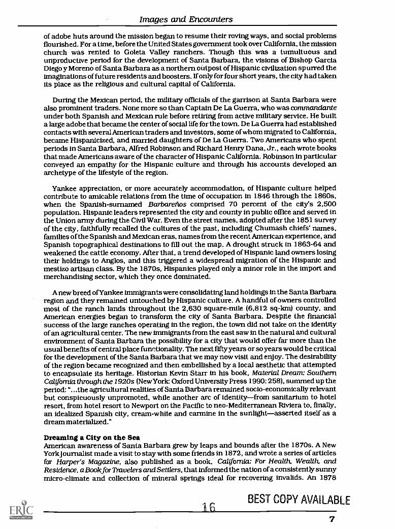
Dreaming a City on the SeaAmerican awareness of Santa Barbara grew by leaps and bounds after the 1870s. A NewYork journalist made a visit to stay with some friends in 1872, and wrote a series of articlesfor Harper's Magazine, also published as a book, California: For Health, Wealth, andResidence, a Bookfor Travelers and Settlers, that informed the nation of a consistently sunnymicro-climate and collection of mineral springs ideal for recovering invalids. An 1878
6BEST COPY AVAILABLE
7
G
o N
ipom
o
LUIS
OB
ISP
O
OU
NT
Y
Tw
itche
llR
eser
voir
Poi
nt S
alM
ar11
Airp
ort
KE
RN
San
ta B
arba
raC
ount
y'L. -
-140
UN
TY
/N
1
i_1
,/L
i11
1
Li
I
Li
(()
i,,
,1-
_N
ew C
uyam
auy
ama
--1_
,L__
_,I
I,..
(,
'--..,
;/
:
(sis
swc
p°,_
i_ci
- \_
r,L
o s
P a
r e
s/
1_1
\V
__, \
iVen
tueo
pe
/"
Z--
N..
/-
Nat
iona
),
1
\/
44., ,z
i,\
----
1,-
,F
ores
t\
-,-,
ek_
-..,
Ak
WI
rig
4 A
,rk L
.,4
RA
CitM
)1T
Y,-
-,
Los
Oliv
os\
Lam
'/
(\
N,
!I
I . 0,
\K:\
=2
H LT-,
. > I
Pur
isim
a P
oint
Los
Ala
mos
ura
Bue
llton
Lake
Cac
hum
a
Poi
ntA
rgue
llo
Gav
iota
Poi
ntC
once
ptio
n
Gol
eta
510
mi
1li
O5
115
km
a c
Oce
anC
oal a
W G
olet
aP
oint
Isla
Poi
ntV
ista
Sum
mer
ianc
i
Car
pint
er`4
19
Rin
conN
Poi
ntP
ita
©19
96 M
AG
ELL
AN
Geo
grap
hixs
m 8
00 9
29-4
MA
Pw
ww
:mag
ella
ngeo
.com
Figu
re 1
.2Sa
nta
Bar
bara
Cou
nty
Ref
eren
ce M
ap
BE
ST C
OPY
AV
AIL
AB
LE
Images and Encounters
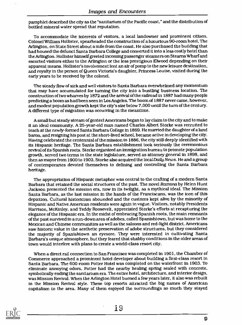
pamphlet described the city as the "sanitarium of the Pacific coast," and the distribution ofbottled mineral water spread that reputation.
To accommodate the interests of visitors, a local landowner and prominent citizen,Colonel William Hollister, spearheaded the construction of a luxurious 90-room hotel, TheArlington, on State Street about a mile from the coast. He also purchased the building thathad housed the defunct Santa Barbara College and converted it into a less costly hotel thanthe Arlington. Hollister himself greeted incoming passenger steamers on Stearns Wharf andescorted visitors either to the Arlington or the less prestigious Elwood depending on theirapparent means. Hollister's involvement lent an air of pomp to the new leisure destination,and royalty in the person of Queen Victoria's daughter, Princess Louise, visited during theearly years to be received by the colonel.
The steady flow of sick and well visitors to Santa Barbara overwhelmed any momentumthat may have accumulated for turning the city into a bustling business location. Theconstruction of two wharves by 1872 and the arrival of the railroad in 1887 had many peoplepredicting a boom as had been seen in Los Angeles. The boom of 1887 never came, however,and modest population growth kept the city's size below 7,000 until the turn of the century.A different type of migration was occurring in the meantime.
A small but steady stream of genteel Americans began to lay claim to the city and to makeit an ideal community. A 25-year-old man named Charles Albert Storke was recruited toteach at the newly-formed Santa Barbara College in 1869. He married the daughter of a landbaron, and resigning his post at the short-lived school, became active in developing the city.Having celebrated the centennial of the mission in 1886, the city still deeply identified withits Hispanic heritage. The Santa Barbara establishment took seriously the ceremoniousrevival of its Spanish roots. Storke organized an immigration bureau to promote populationgrowth, served two terms in the state legislature, served as attorney general in 1898, andthen as mayor from 1900 to 1902. Storke also acquired the localDaily News. He and a groupof contemporaries devoted themselves to defining and controlling the Santa Barbaraheritage.
The appropriation of Hispanic metaphor was central to the crafting of a modern SantaBarbara that retained the social structures of the past. The novel Ramona by Helen HuntJackson presented the mission era, now in its twilight, as a mythical ideal. The MissionSanta Barbara, as the last mission in the hands of the Franciscans, was the icon of thisdepiction. Cultural historicism abounded and the customs kept alive by the minority ofHispanic and Native American residents were again in vogue. Visitors, notably PresidentsHarrison, McKinley, and Teddy Roosevelt, appreciated Storke's efforts at recapturing theelegance of the Hispanic era. In the midst of embracing Spanish roots, the main remnantsof the past survived in a run-down area of adobes, called Spanishtown, but was home to theMexican and Chinese communities as well as the saloons and red-light district. Americanssaw historic value in the aesthetic preservation of adobe structures, but they consideredthe majority of Spanishtown an eyesore. They were interested in cultivating SantaBarbara's unique atmosphere, but they feared that shabby conditions in the older areas oftown would interfere with plans to create a world-class resort city.
When a direct rail connection to San Francisco was completed in 1901, the Chamber ofCommerce approached a prominent hotel developer about building a first-class resort inSanta Barbara. The 600-room Potter Hotel was completed on the waterfront in 1903. Toeliminate annoying odors, Potter had the nearby healing spring sealed with concrete,symbolically ending the sanitarium era. The entire hotel, architecture, and interior design,was Mission Revival. When the Arlington Hotel burned a few years later, it also was rebuiltin the Mission Revival style. These top resorts attracted the big names of Americancapitalism to the area. Many of them enjoyed the surroundings so much they stayed
1 0
Santa Barbara and California's Central Coast Region
permanently and built estates. Climate and beauty attracted this new class of resident aswell as the opportunity to connect with an air of aristocracy. They expressed their idealsinarchitecture and art, and also in lifestyle, with much yachting, riding, polo, and golf. Theyconstructed grand seasonal mansions in Mediterranean motifs, primarily in the hills ofMontecito. The wealthy families that staked an interest in and around Santa Barbara wouldplay important roles in imagining and realizing a city that would fulfill their fanciful dreamsand selective history. An echo of a long-dead bishop's grand plans, the construction of St.Anthony's Seminary alongside a restored mission in 1901 also helped to ensure that a once -jeopardized past would remain current.
The final chapter of Santa Barbara's development began in 1909, when the Civic Leagueof Santa Barbara brought in planner Charles Robinson to propose a master plan for the city.Robinson's suggestion was to develop the dramatic, topographically unique site into acohesively conceived and aesthetically engineered presentation of history. He saw theMission and the historic Plaza de la Guerra as the symbols for the city, and recommendedthat the undistinguished public buildings of the civic center be torn down and replaced. Themission and plaza should be framed by a number of landscaped vistas and surrounded bya network of public spaces. Museums to display the city's heritage were also included in theplans. Industrial development was seen as polluting and to be avoided. Robinson's costlyand bold recommendations were received and accepted, but nonetheless forgotten. Theplan, however, was popular with the local elite who constituted the Civic League. As theyears passed and local power shifted into the hands of those elite, Santa Barbara's futurewould be sculpted to look more and more like Robinson's vision.
On its way to establishing its identity, the city had been presented with manyopportunities, which for one reason or another had not worked out. Early in the twentiethcentury, a Navy presence similar to that which eventually located in San Diego and LongBeach was one possibility. City officials were unenthusiastic about the prospects of aconstant sailor population, and the Navy chose other ports for expanding its Pacificoperations. The aviation industry also arrived on the local scene. During World War I, threebrothers named Loughead (they would later change the spelling to Lockheed) employedeighty-five locals, including one Jack Northrop, to manufacture seaplanes. For a shortperiod the focus of the flying world was on the South Coast, but the brothers eventuallymoved their operation to Los Angeles in the 1920s. The resorts also opened the door foranother industry, filmmaking, which came to town as early as 1910. The world's largestmovie studio was built downtown in 1913. Called the "Flying A," the facilities hosted fourteenfilm companies and produced more than 2,000 major films during the next eightyears. By1921, however, the industry had moved south in search of new filming locations, and thestudio was finally destroyed in 1948.
Unperturbed by these transitions in industry, a collection of artists began to colonizeSanta Barbara including painters in the plein air tradition that valued the quiet andpastoral settings of the region. Horticulturists and wildlife enthusiasts also flowed intoSanta Barbara. Another group of painters celebrated the disappearing Old West. The SantaBarbara School of the Arts was opened in the 1920s, and a circle of the artistic elite aroseas it did in Santa Fe and Taos, New Mexico. A number of myths, including that of Zorro, werecreated that invented and capitalized on an image of Santa Barbara life. Citizens of the citywere enthralled with the image and sought to embrace and foster it in any way possible.Subdivisions were built to attract wealthy people who wanted to attach themselves to thelifestyle and the lifestyle to themselves. Many celebrities including Mary Pickford andDouglas Fairbanks, Jr. (Zorro himself) made Santa Barbara their home.
The Community Arts Association during the 1920s emerged as the agent responsible forguarding the identity of the city. Under the guidance of prominent citizens, the group beganby holding pageants and celebrations to promote Hispanic culture. The group then movedon to the appearance of the city. Money was collected among virtually all of the wealthy
20
10
Images and Encounters
residents, and aesthetically inclined leaders directed its expenditure on projects designedto beautify the city and preserve (and in some cases recreate) its Hispanic heritage. At theurging of the committee, the city formed a Planning Commission in 1923. Although thePlanning Commission was not able to push through a grand comprehensive plan developedin cooperation with Olmsted and Olmsted of New York, it was able to pass a comprehensivebuilding code for the city. A competition was held for small house designs appropriate forthe Santa Barbara image and costing no more than $5,000 to build. The Community ArtsAssociation published the selected designs. In addition, the few remaining historic adobesworthy of restoration were purchased and restored by members of the community.
Built between 1922 and 1924, the El Paseo, a downtown shopping complex, was asignificant addition to Santa Barbara architecture. Designed as a street in Spain, thecomplex attached itself to the authenticity of the Plaza de la Guerra, which had for some timebeen neglected. It was a form of recycled history that was decidedly popular with localresidents. Another project, to provide the city with a theater and opera house, used part ofan historic adobe structure in the configuration of a new theater, the Lobero, which alsoincorporated the essence of Spanish revival.
In the midst of this redecoration of the city along historical, if significantly modified andupdated, standards received an unexpected boost when on 29 June 1925, an earthquakeleveled much of the city. Though only twelve of 25,000 residents perished, the damage wasdevastatingunless you had been wanting to tear it all down anyway. The newconstruction, like the El Paseo complex, the Lobero Theater, theDaily News building on thehistoric plaza, and the homes built according to the new standards, survived the incident,but the older buildings downtown and the mission itself were severely weakened. As far asthe Community Arts Association was concerned, the mistakes of the nineteenth and earlytwentieth centuries had been erased in one fell swoop. The Association's Plans andPlantings Committee was ready for the rebuilding. JuSt at the time of the earthquake, thecommittee had pushed through a measure creating a Board of Architectural Review. For thefirst time in California, and perhaps the United States, preservationists, planners, andaesthetes had gained control of a city and were putting their distinctive mark on it.
The rest of the country noted how quickly and decisively Santa Barbara was beingrebuilt. The formerly unsightly spine of State Street was now becoming a downtown stripworthy of one of the world's most beautiful cities. A symbol of Santa Barbara's vision andwealth, the third County Courthouse, completed in 1929, became the centerpiece of thereborn city. Built in the image of a castle in Spain and costing nearly two million dollars,it was touted as the world's most beautiful jail. Details of the building, like 14,000 squarefeet of floor tile and a mural depicting the history of the area from the first Spanish landing,ensured that the Hispanic metaphor would remain powerful. Throughout the state andamong the local elite, money was raised to fund the $400,000 project to restore the mission.At the same time, Major Max Fleischmann (of yeast fame) was single-handedly securing theconstruction of a breakwater that was necessary to create safe harbor for his 250-foot yachtand other pleasure craft that residents wished to keep. He contributed more than $600,000to complete the project near Stearns Wharf. Fleischmann also established the SantaBarbara Foundation, which worked devotedly to preserve the buildings and landscapesthat projected the much sought after Hispanic aesthetic.
The enthusiastic and able involvement of the private sector in Santa Barbara is what hasallowed it to emerge as an extraordinarily endowed smaller city. Time magazine would referto Thomas Storke in the 1930s as the benevolent dictator of Santa Barbara. Individuals likeStorke have seen in Santa Barbara something so appealing, even mesmerizing, that theyhave made it their own. That is why, when you tour around the city, you are left wonderinghow it, among so many cities of this country, has been able to uphold a dignity and aestheticbeauty that has become so uncommon in our world of temporary landscapes and industrialwastelands. Much has happened in the city since the 1930s, but it can be said with
2111
Santa Barbara and California's Central Coast Region
confidence that what has occurred since this time has always been in line with thevalues of the visionaries who saw the opportunity to make on the west coast of theUnited States a dazzling Spanish town. It is here for you to see and experience. Unlikeother cities, Santa Barbara does not cover up and abandon its past. If anything itseizes the past, takes from it what it desires, and brings that imaginary conceptionto life in a real city.
This is only a small part of the story of Santa Barbara. It is better for you to discoverit for yourself. I have tried to reveal the origin of the image that ties the myth andmaterial of the city together. Mention Santa Barbara and, as travel writer CharlesStephen Brooks observed in 1935, it is likely that the excited eye of your fancy...willalight on marbled pools and stairways, on Spanish houses that out-castle thepalaces of Europe, on Satin apartments larger than a city railway station where awhole company at dinner could be swallowed by lofty walls without the slightestwiggle of their gilded Adam's apples," (quoted in Starr 1990: 302). That is a bitextreme, but it entitles Santa Barbara to be called "The American Riviera."
22
12
Images and Encounters
2
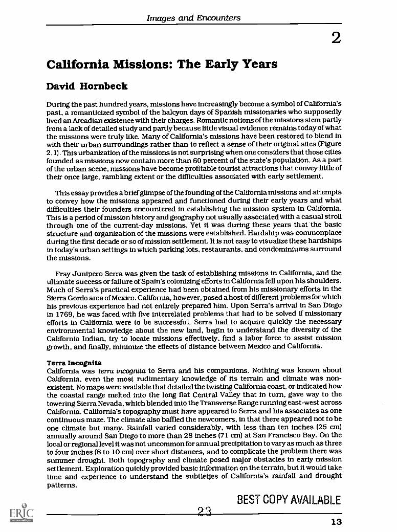
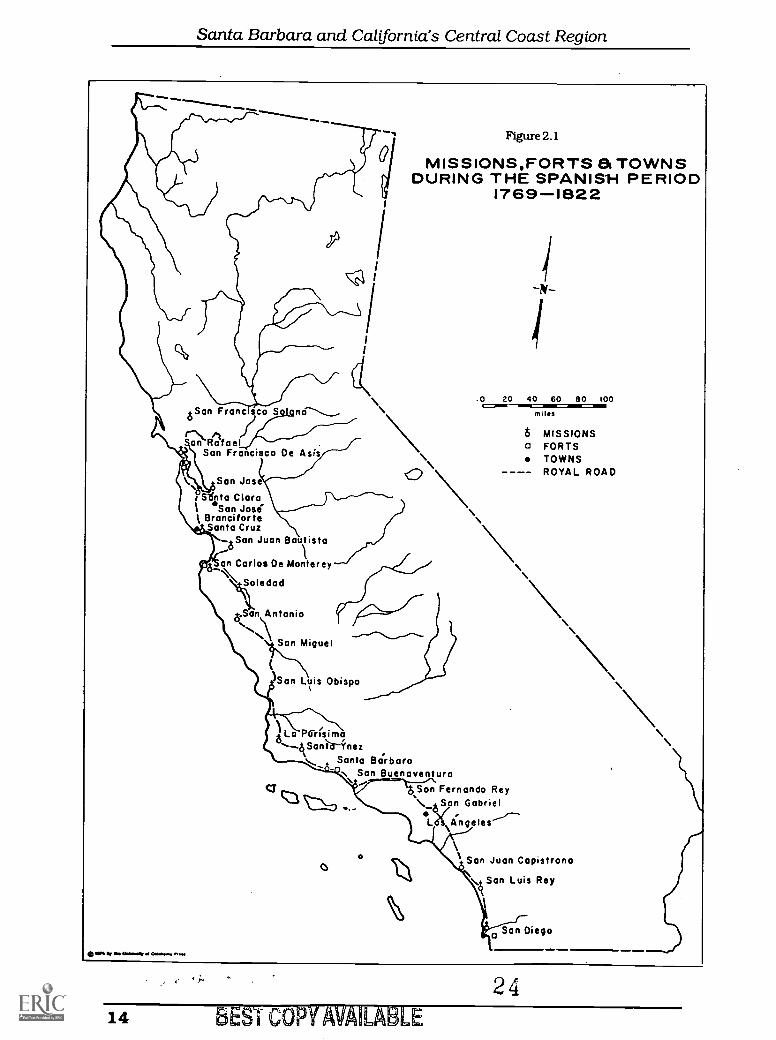
California Missions: The Early YearsDavid HornbeckDuring the past hundred years, missions have increasingly become a symbol of California'spast, a romanticized symbol of the halcyon days of Spanish missionaries who supposedlylived an Arcadian existence with their charges. Romantic notions of the missions stem partlyfrom a lack of detailed study and partly because little visual evidence remains today of whatthe missions were truly like. Many of California's missions have been restored to blend inwith their urban surroundings rather than to reflect a sense of their original sites (Figure2.1). This urbanization of the missions is not surprising when one considers that those citiesfounded as missions now contain more than 60 percent of the state's population. As a partof the urban scene, missions have become profitable tourist attractions that convey little oftheir once large, rambling extent or the difficulties associated with early settlement.
This essay provides a brief glimpse of the founding of the California missions and attemptsto convey how the missions appeared and functioned during their early years and whatdifficulties their founders encountered in establishing the mission system in California.This is a period of mission history and geography not usually associated with a casual strollthrough one of the current-day missions. Yet it was during these years that the basicstructure and organization of the missions were established. Hardship was commonplaceduring the first decade or so of mission settlement. It is not easy to visualize these hardshipsin today's urban settings in which parking lots, restaurants, and condominiums surroundthe missions.
Fray Junipero Serra was given the task of establishing missions in California, and theultimate success or failure of Spain's colonizing efforts in California fell upon his shoulders.Much of Serra's practical experience had been obtained from his missionary efforts in theSierra Gordo area of Mexico. California, however, posed a host of different problems for whichhis previous experience had not entirely prepared him. Upon Serra's arrival in San Diegoin 1769, he was faced with five interrelated problems that had to be solved if missionaryefforts in California were to be successful. Serra had to acquire quickly the necessaryenvironmental knowledge about the new land, begin to understand the diversity of theCalifornia Indian, try to locate missions effectively, find a labor force to assist missiongrowth, and finally, minimize the effects of distance between Mexico and California.
Terra IncognitaCalifornia was terra incognita to Serra and his companions. Nothing was known aboutCalifornia, even the most rudimentary knowledge of its terrain and climate was non-existent. No maps were available that detailed the twisting California coast, or indicated howthe coastal range melted into the long flat Central Valley that in turn, gave way to thetowering Sierra Nevada, which blended into the Transverse Range running east-west acrossCalifornia. California's topography must have appeared to Serra and his associates as onecontinuous maze. The climate also baffled the newcomers, in that there appeared not to beone climate but many. Rainfall varied considerably, with less than ten inches (25 cm)annually around San Diego to more than 28 inches (71 cm) at San Francisco Bay. On thelocal or regional level it was not uncommon for annual precipitation to vary as much as threeto four inches (8 to 10 cm) over short distances, and to complicate the problem there wassummer drought. Both topography and climate posed major obstacles in early missionsettlement. Exploration quickly provided basic information on the terrain, but it would taketime and experience to understand the subtleties of California's rainfall and droughtpatterns.
13
BEST COPY AVAILABLE
13
Santa Barbara and California's Central Coast Region
1141
Figure 2.1
MISSIONS,FORTS &TOWNSDURING THE SPANISH PERIOD
1769-1822
NM
San Jos
r Slinto Clara1 San Jose \t Brancitorte \
Santa Cruz-San Juan Bautista
an Carlos De Monterey
Soledad
.0 20 40 60 BO 100
miles
6 MISSIONS0 FORTS
\ TOWNSROYAL ROAD
8. an Antonio
San Miguel
San Luis Obispo
)La PGrisimaS a e z
Santo BrirbaraSan Buenaventura
C:t kSan Fernando Rey\ San GabrielidL
OSan Juan Capistrano
.,6 San Luis Rey
Son Diego
2414 EsESI COPY AVAILABLE
Images and Encounters
The environment, however, was not the only immediate problemfacing Serra. Chargedwith establishing missions that were to acculturate the Indian, Serra and his companionsfound the Indians to be as diverse and as bewildering as their environment. In 1769,California contained approximately 310,000 Indians scattered throughout the state,withdensities ranging from very high along the coast to very low in the interior. The newcomerswere surprised that California Indians did not practice agriculture but instead werehunters and gatherers. The most significant aspect of the California Indian was language.California was a virtual Babel of mutually unintelligible tongues. ThroughoutCalifornia sixlanguage stocks existed along with approximately fourteen language families, and abouteighty mutually unintelligible tongues, all divided into more than 300 dialects.The humanlandscape was a mosaic of hundreds of small, autonomous groups, each differingfrom itsneighbor in speech, and quite frequently, in custom.
Both the physical and human landscapes were difficult to understand at first, yet alongwith the military commander, Serra was charged with the responsibility of foundingmissions. The problem was that missions were to be founded before the new settlers couldobtain much environmental knowledge. Specific site requirements for new missions werelarge numbers of Indians, available water, flat land for planting and harvesting crops,abundant building materials, and accessibility. The success of mission settlementdepended on how well the newcomers could identify and understand these locationalfactors. At the outset, availability of water proved to be the most crucial factor, San Diego,San Carlos, and San Antonio were moved because their initial sites lacked sufficient waterfor agriculture. In all, six of the first nine missions had to be moved, illustrating thatenvironmental knowledge was acquired slowly and by painful experiences. (Floodingoccurred when 1812 earthquakes caused failure of the dam holding back water in areservoir in the mountains above the La Purisima mission, and the mission was relocatedthree miles away from its original site in what is today the city of Lompoc in Santa BarbaraCounty. Scars from that event are still visible from-the ruins of the original mission site.)
Once missions were established, a new problem of labor surfaced. An adequate laborsupply was an important foundation upon which rested the spiritual and economic successof the mission. Although considerable attention was given to the number ofIndians livingnear a proposed mission site, the local Indians proved inadequate to provide the neededsupply of labor. There was a reciprocal relationship between conversion of Indians and laborsupply. The introduction of Indians into the mission required a constant food supply, yetfood production demanded a constant labor supply. This "catch 22" was a critical problemfor the missions because the Indians had to be taught the necessary agricultural or buildingskills to support the mission. Without an ongoing food supply, Indians could notbe attractedto the missions and without Indians, the mission inhabitants could not plant and harvestcrops.
Distance and LocationIn addition to the difficulties already discussed, distance posed an immediate and seriousobstacle to mission settlement. Hundreds of miles of unexplored desert and an unknownnumber of possible hostile Indians separated California and the nearest Spanishsettlements in Sonora, Mexico. The only practical way to maintain the California outpostwas by a tenuous sea route that extended well over one thousand miles (1600 Ian) back toMexico.
Isolated in a new environment, Serra and his missionaries found themselves groping tosolve unfamiliar problems. The handful of missionaries were too few tomake more than afeeble effort to occupy the land. Equipment, food, and labor were in short supply or non-existent. The Indian could not be relied upon for food or labor as had been the custom onearlier frontiers. A combination of problems, therefore, made mission settlementproblematic, to say the least. By 1774, the missions were scarcely more than tenuous signsof Spanish occupance.
2515
Santa Barbara and California's Central Coast Region
Mission Settlement and EvolutionAs the previous discussion suggests, the missionswere not easily implanted on theCalifornia landscape. Mission settlement finally overcame many of the problems.Slowly during their 65-year tenure in California, missionaries created complicatedirrigation systems, constructed new buildings, expanded crops and livestock, andcreated new land uses that remain a part of California's geographical heritage.
A stroll through the Santa Barbara Mission today would reveal little of thehardships encountered in its establishment. Cultivated fields that once representedthe first signs of success in a new land are now covered by condominiums. Irrigationditches, so vital to the mission's survival, lie buried under parking lots, and officebuildings now stand in the place of the Indian villages that housed the mission's hardwon labor force. The missions easily fit into this urban milieu because they have notbeen restored to reflect either the hardships of the past or authentic day-to-daymission life. Missions are clean, almost antiseptic in their appearance and projectthe image of what we think they should have looked like had they been founded inthe twentieth century. Today our missions make few statements about themselvesthey blend into the urban scene and tell us more about ourselves than they do aboutthe past.
26
16
Images and Encounters
Califon-1d, Populsidona
3
The last 95 years have witnessed a remarkable transformation of California's landscapesas the plains have been irrigated and great cities have sprung up where only villagesformerly existed. In large measure, the remaking of the land has been a direct result ofimmigration and rapid population growth. At the beginning of the twentieth century,1,485,053 persons resided in the state and only a quarter of a million people lived in the fivecounties that make up the Los Angeles Basin.
TransformatIon off the Cantonal& Lamle IlseapeThe expansion of modern irrigated agriculture coupled with the growth of the petroleum,entertainment, aerospace, and electronics industries soon attracted an apparently endlessstream of newcomers. During the first three decades, the basin's population doubled everyten years, so that by 1930 almost half of California's 5,677,251 people resided in the south.Neither economic depression nor war would materially slow the flow of people.
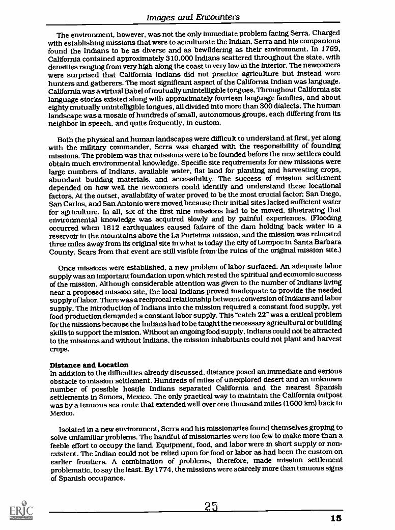
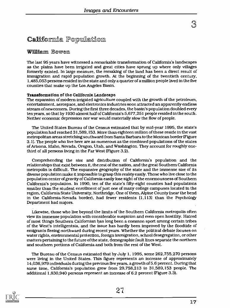
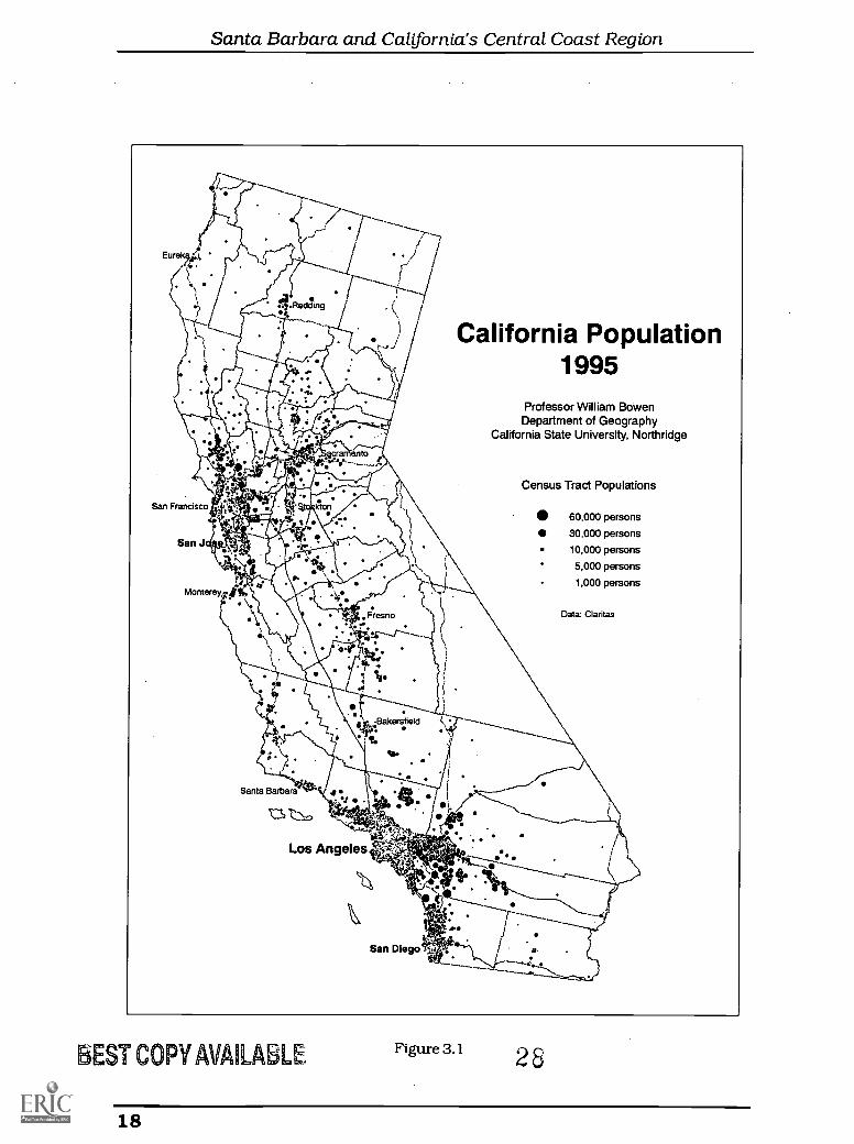
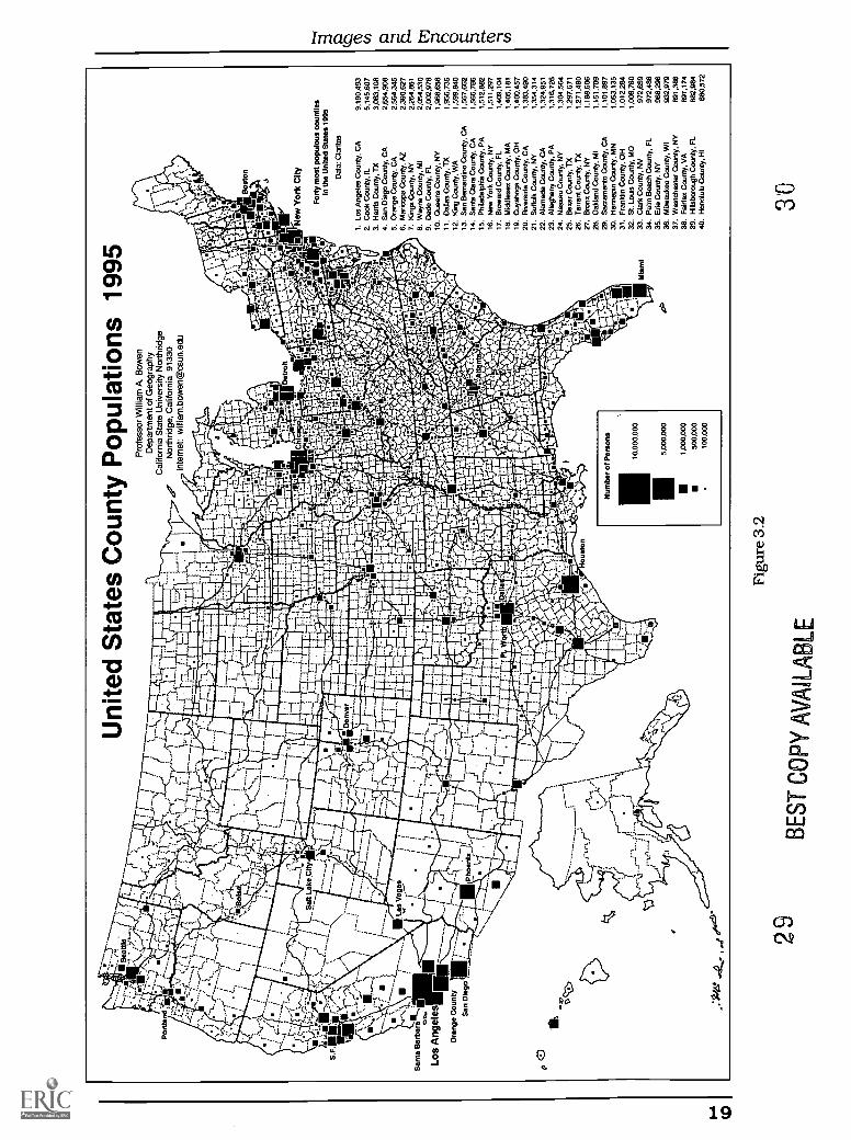
The United States Bureau of the Census estimated that by mid-year 1995, the state'spopulation had reached 31,589,153. More than eighteen million of these reside in the vastmetropolitan areas stretching southward from Santa Barbara to the Mexican border (Figure3.1). The people who live here are as numerous as the combined populations of the statesof Arizona, Idaho, Nevada, Oregon, Utah, and Washington. They account for roughly one-third of all persons living in the Far West (Figure 3.2).
Comprehending the size and distribution of California's population and therelationships that exist between it, the rest of the nation, and the great Southern Californiametropolis is difficult. The expansive geography of the state and the immense size of itsdiverse population make it impossible to grasp this reality easily. Those who live close to thepopulation center of gravity of California easily lose sight of the enormousness of SouthernCalifornia's population. In 1990, ten of the state's fifty-eight counties had populationssmaller than the student enrollment of just one of many college campuses located in theregion, California State University, Northridge. One of them, Alpine County (near the bendin the California-Nevada border), had fewer residents (1,113) than the PsychologyDepartment had majors.
Likewise, those who live beyond the limits of the Southern California metropolis oftenview its immense population with considerable suspicion and even open hostility. Hatredof most things Southern Californian has long been a common sport among certain tribesof the West's intelligentsia, and the issue has hardly been improved by the floodtide ofemigrants fleeing northward during recent years. Whether the political debate focuses onwater rights, environmental protection, foreign immigration, school desegregation, or othermatters pertaining to the future of the state, demographic fault lines separate the northernand southern portions of California and both from the rest of the West.
The Bureau of the Census estimated that by July 1, 1995, some 262,755,270 personswere living in the United States. This figure represents an increase of approximately14,036,979 individuals during the previous five years, a growth of 5.6 percent. During thatsame time, California's population grew from 29,758,213 to 31,589,153 people. Theadditional 1,830,940 persons represent an increase of 6.2 percent (Figure 3.3).
26.
I.7
Santa Barbara and California's Central Coast Region
_7'. r-------7---1
1 /1--'
f
f.----,.
) / California Population,/ 1995ii
7 Professor William BowenDepartment of Geography
California State University, Northridge
Census Tract Populations
60,000 persons
30,000 persons
10,000 persons
5,000 persons
1,000 persons
Data: Claritas
Los Angeles
BEST COPY AVAILABLEFigure 3.1 2
18
Por
tland
to
..--.
en
.
Sea
ttle I
- r- -7`
Uni
ted
Sta
tes
Cou
nty
Pop
ulat
ions
199
5P
rofe
ssor
Will
iam
A. B
owen
Dep
artm
ent o
f Geo
grap
hyC
alifo
rnia
Sta
te U
nive
rsity
Nor
thrid
ge
.-,f
Nor
thrid
ge, C
alifo
rnia
913
30in
tem
et: w
illia
m.b
owen
@cs
un.e
du
S,y
\V
oi 4
.
1%S
anta
Bar
bara
?.
Ififf.
P5
3-1
7
A.,-
:-7,
174r
illit
%rin
gN
iirfy New
Yor
k C
ity
Los
Ang
eles
Ora
nge
Cou
nty
San
Die
go
0 0
Hou
ston
Num
ber
of P
erso
ns
10,0
00,0
00
5,00
0,00
0
1,00
0,00
0
500,
000
100,
000
For
ty m
ost p
opul
ous
coun
ties
In th
e U
nite
d S
tate
s 19
95
Dat
a: C
larit
as
1. L
os A
ngel
es C
ount
y, C
A2.
Coo
k C
ount
y, IL
3. H
arris
Cou
nty,
l'X
4. S
an D
iego
Cou
nty,
CA
5. O
rang
e C
ount
y, C
A6.
Mal
icop
a C
ount
y, A
Z
7.W
ayne
7.tG
ngsn
eC
ount
y,N
Y MI
9. D
ade
Cou
nty,
FL
10. Q
ueen
s C
ount
y, N
Y11
. Dal
las
Cou
nty,
DC
12. K
ing
Cou
nty,
WA
13. S
an B
erna
rdin
o C
ount
y, C
A14
. San
ta C
lara
Cou
nty,
CA
15. P
hila
delp
hia
Cou
nty,
PA
16. N
ew Y
ork
Cou
nty,
NY
17. B
row
ard
Cou
nty,
FL
18. M
iddl
esex
Cou
nty,
MA
19. C
uyah
oga
Cou
nty,
OH
20. R
iver
side
Cou
nty,
CA
21. S
uffo
lk C
ount
y, N
Y22
. Ala
med
a C
ount
y, C
A23
. Alle
ghen
y C
ount
y, P
A24
. Nas
sau
Cou
nty,
NY
25. B
evy
Cou
nty,
TX
26. T
arra
nt C
ount
y, D
C27
. Bro
nx C
ount
y, N
Y28
. Oak
land
Cou
nty,
MI
29. S
acra
men
to C
ount
y, C
A30
. Hen
nepi
n C
ount
y, M
N31
. Fra
nklin
Cou
nty,
OH
32. S
t. Lo
uis
Cou
nty,
MO
33. C
lark
Cou
nty.
NV
34. P
alm
Bea
ch C
ount
y, F
L35
. Erie
Cou
nty,
NY
36. M
ilwau
kee
Cou
nty,
WI
37. W
estc
hest
er C
ount
y, N
Y38
, Fai
rfax
Cou
nty,
VA
39. H
illsb
orou
gh C
ount
y, F
L40
. Hon
olul
u C
ount
y, H
I
9,19
0,49
35,
145,
607
3,08
3,10
82,
654,
908
2,56
4,34
52,
390,
627
2,26
4,86
12,
054,
530
2,00
2,97
81,
966,
658
1,95
6,73
51,
599,
840
1,56
7,66
21,
566,
786
1,51
2,88
21,
511,
297
1,40
9,10
41,
405,
181
1,40
0,45
71,
383,
490
1,35
4,31
41,
324,
951
1,31
6,72
61,
304,
564
1,29
7,67
11,
271,
480
1,18
8,60
61,
151,
709
1,10
1,89
71,
053,
135
1,01
2,28
41,
006,
760
972,
659
972,
486
966,
296
932,
979
891,
386
891,
174
882,
984
880,
572
29B
EST
CO
PYA
VA
ILA
BL
E
Figu
re 3
.2
30
Santa Barbara and California's Central Coast Region
R48$1821;353gPPMTSSS3S2G2G8
20
Population GrowthAlthough not matching the levels of growth witnessed in previous decades, the increase isaltogether remarkable given the fact that California has begun experiencing the greatestexodus of residents from any state in our nation's history. Its 1993 to 1994 netdomestic out-migration rate reached 1.4 percent, the highest of any state, and represented a net loss of426,000 migrants to other states. The Census Bureau estimates that between 1990 and2020, California will sustain a net loss of four million internal migrants to other states. Thistremendous loss, however, is expected to be more than offset by the arrival often million newinternational migrants (39 percent of the nation's total) and more than twice as many birthsas deaths (20 million versus 8 million).
Most of the newcomers have not yet sought a lasting political affiliation with the new land.Recent estimates reveal that in the entire state approximately 5,960,000 were non-citizensin 1994, 3,852,000 from Latin America and 1,253,000 from nations bordering the westernrim of the Pacific Ocean. More than 98 percent of these new arrivals have settled in themetropolitan areas of the state, 2,706,000 (45.4 percent) in large central cities and3,150,000 (52.8 percent) in the more suburban areas and smaller cities. By far the greaternumber of these people have chosen to make their new homes in the Los Angeles Basin.Their numbers simply dwarf those measured elsewhere in the United States.
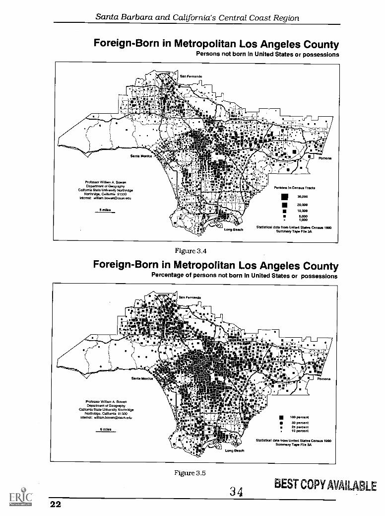
Influence of ImmigrantsBy 1994, approximately 25 percent of the state's population were foreign immigrants.Among the adult population the percentage was considerably higher. One effect of these twomigration streams was the creation of a multi-national metropolis in Southern Californiaalmost overnight. By 1990, more than 38 percent of all adults in Los Angeles County wereforeign-born (Figures 3.4 and 3.5). In broad areas of the Los Angeles Basin encompassingmany scores of square miles, the majority of adults are no longer Americans by birth ornaturalization. In some neighborhoods immediately west of downtown Los Angeles thepercentages exceed 90 percent! More than 100 foreign languages are spoken by childrenattending Los Angeles City schools. The America known to politicians from Arkansas andKansas is remote, unknown, and hardly even relevant.
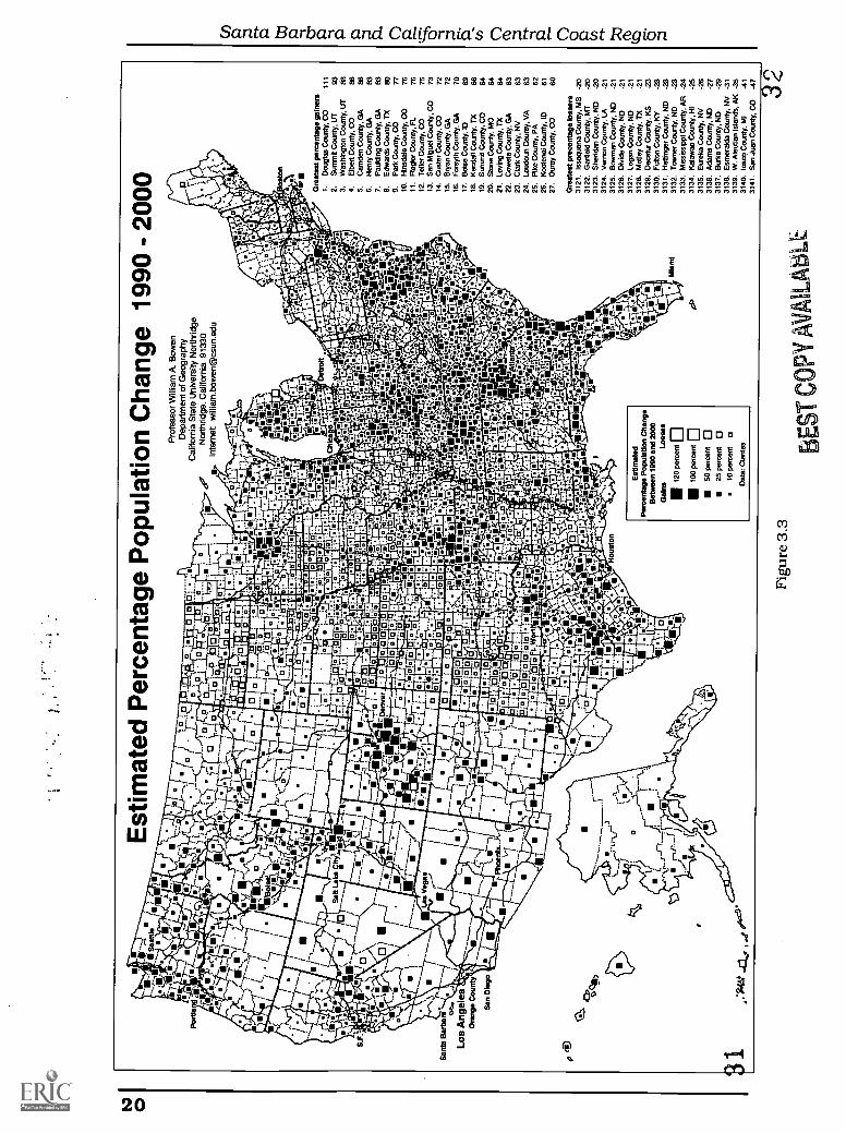
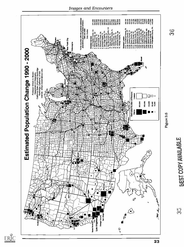
By the end of this century, the Claritas Corporation estimatesthat 275,392,233 personswill reside in the United States, a gain of 26,682,360 individuals during the 1990s. Thisincrease will be distributed unevenly across the nation. All 25 of the counties gaining thelargest number of new inhabitants will be located in the West or South. Those countiessuffering the greatest losses will be, with a few exceptions, the locations of aging nineteenthcentury cities such as Philadelphia; Detroit, Washington, D.C., and Baltimore. Smaller, butoften desperately significant, declines are occurring in approximately 21 percent of countiesin the United States. Most of these are located in the rural lands of the Great Plains andUpper Middle West.
Five of the nation's top ten counties witnessing the greatest population increases will belocated in Southern California. Two others will be located nearby in Nevada(Clark County-Las Vegas) and Arizona (Maricopa County-Phoenix). The only California county toexperience a significant decline in population will be Monterey (central coast of California),where major economic dislocations have occurred already as a result of the closure of FortOrd.
Although metropolitan Southern California exceeds all other areas of the nation in thesheer size, scope, and visibility of its population growth, the percentages at which itscounties are growing today are relatively small. It is extraordinarilydifficult to sustain highpercentages of growth in already large populations. How much simpler it is to double the sizeof a rural county's population with the development of several large, new subdivisionsacross the line from a neighboring city. Douglas County, Colorado is a case in point. It liesimmediately to the southwest of Denver and has recently been invaded by suburbanites.
3 3 BEST COPY AVAILABLE
21
Santa Barbara and California's Central Coast Region
Foreign-Born in Metropolitan Los Angeles CountyPersons not born in United States or possessions
San Fernando
/-
Professor William A. BowenDepartment of Geography
Califomia State University NorthridgeNorthridge, California 91330
internal: [email protected]
5 miles
Long Beech
Persons In Census Tracts
111130,000
20,000
10,000
5,0001,000
Statistical data from United States Census 1990Summary Tape File 3A
Figure 3.4
Foreign-Born in Metropolitan Los Angeles CountyPercentage of persons not born in United States or possessions
Sen Fernando
Santa Monica
Professor William A. BowenDepartment of Geography
California State University NorthridgeNorthridge, California 91330
intemet: [email protected]
5 miles
Long Beach
100 percent
50 percent25 percent10 percent
Statistical data from United States Census 1990Summary Taps File 3A
Figure 3.5
34 BEST COPY AVAILABLE
22
7-2. 'N
I...
, -
Port
lend
li. ._,
''l *
.k.h
.7
1--1
-i-
'
". e
-Z-; -
-I
---,
'1
_-,
'?"1 , -
.!.
).
,
f%
,I
"Est
imat
ed P
opul
atio
n C
hang
e 19
90 -
200
0P
rofe
ssor
Will
iam
A. B
owen
jalf
Dep
artm
ent o
f Geo
grap
hy
r--c
"r-"
"-N
s.,,,
,C
allfo
rnia
Sta
te U
nive
rsity
Nor
thrid
ge
..1.1
. -^1
Nor
thrid
ge, C
alifo
rnia
913
30in
tem
et: w
illia
m.b
owen
gcsu
n.ed
u
S.F.
VII
IIW
NM
I
Sant
a B
arbe
ra
Los
Ang
eles
11-= "1
1O
rang
e C
ount
y'M
INSa
n D
iego
"...
f
5T
.%H
oust
on
Est
imat
ed N
umbe
r of
Per
sons
600,
000
300.
000
100,
000
50,0
0010
,000
Los
ses n 0 0 0
Bos
ton
New
Yor
k C
ity
Phila
delp
hia
Thi
rty
coun
ties
with
the
grea
test
est
imat
edpo
pula
tion
gain
s an
d lo
sses
bet
wee
n19
90 a
nd 2
000
Dat
a: Q
anta
s
Gre
ates
t Gai
ners
1. L
os A
ngel
es C
ount
y, C
A57
7,30
62.
Mar
icop
a C
ount
y, A
Z56
5,00
43.
Har
ris
Cou
nty,
TX
525,
806
4. C
lark
Cou
nty,
NV
470,
163
5. R
iver
side
Cou
nty,
CA
413,
284
6. B
row
ard
Cou
nty,
FL
302,
037
7. S
an D
iego
Cou
nty.
CA
296,
976
8. O
rang
e C
ount
y, C
A28
7,35
99.
San
Ber
nard
ino
Cou
nty,
CA
262,
013
10. B
exar
Cou
nty,
TX
228,
011
11. P
alm
Bea
ch C
ount
y, F
L21
2,59
412
. Dal
las
Cou
nty,
TX
205,
299
13. T
arra
nt C
ount
y, T
X20
0,57
114
. Gw
inne
tt C
ount
y, G
A19
5,85
815
. Hid
algo
Cou
nty,
TX
186,
438
Gre
ates
t Los
ers
3127
. Pro
vide
nce
Cou
nty,
RI
3128
. Har
tfor
d C
ount
y, C
T31
29. O
rlea
ns C
ount
y, L
A31
30. E
ssex
Cou
nty,
NJ
3131
. Bro
nx C
ount
y, N
Y31
32. N
orfo
lk C
ount
y, V
A31
33. A
llegh
eny
Cou
nty,
PA
3134
. Milw
auke
e C
ount
y, W
I31
35. S
t. L
ouis
Cou
rtly
, MO
3138
. Suf
folk
Cou
nty,
MA
3137
. fen
gs C
ount
y, N
Y31
38. B
altim
ore
Cou
nty,
MD
3139
. Dis
tric
t of
Col
umbi
a
-28,
160
-30,
324
-30,
432
-30,
765
32,7
9441
,062
-42,
898
-53,
573
-63,
753
-67,
579
-75,
839
-79.
277
.80,
856
3140
. Way
ne C
ount
y, M
l-1
17,0
9331
41. P
hila
delp
hia
Cou
nty,
PA
-14
3,50
6
35B
EST
CO
PYA
VA
ILA
BL
E
Fig
ure
3.6
36
Santa Barbara and California's Central Coast Region
Many members of America's wealthy and highly educated classes dream of a "RockyMountain high." Thousand have invaded the mountain communities of Colorado to live it.
Migration FlowsHigh percentages of growth can indicate the direction of migratory flows. Hundreds ofthousands of Californians, many of them retirees, have fled this state bound for what theyhope is a better future in the towns of the Pacific Northwest and the Rocky Mountain states.Others from throughout the nation have chosen the suburbs of Atlanta; Washington, D. C.;Denver; and a score of other favored destinations. The Gulf Coast counties of Alabama andFlorida have their attraction to some. For others migrating northward from Mexico, thesouthwestern border counties are at least satisfactory immediate destinations. Not all of theUnited States will increase in population. Few counties in the Great Plains have been ableto sustain themselves. The lucky few sit on major transcontinental freeways or gas fields.Iowa farmers are diminishing in numbers. So also are the number of people willing to liveon the flood plains of the Mississippi River.
The California situation follows national patterns. Some sparsely settled sections of thestate are being brought within the web of modern urban life. Formerly small communitiesin the foothills of the Sierra Nevada east of Sacramento are experiencing high rates ofgrowth, as are many Central Valley towns and cities such as Fresno, Bakersfield, Manteca,Yuba City, and Redding. As always, new communities are forming along the inland edges ofthe state's two great urban centersLos Angeles and San Francisco.
The Future?Projecting California's population into the more distant future is a task fraught with manyuncertainties (Figure 3.6). The Census Bureau estimates that within 25 years California'sresidents will number 47,953,000 and account for 15 percent of the nation's population.Many of these will be the millions of new immigrants now arriving from lands touching thePacific and Indian Oceans, people who are fleeing their impoverished homelands in searchof better lives.
The future of California and its people is increasingly affected by unreported eventsoccurring in far distant lands. The growth of an increasingly globalized economy and thedevelopment of new transportation and communications technologies bind our fate evercloser to the many peoples who live beyond our national, state, and regional borders. Weshould not lose sight, therefore, of the most ignored story of this century, the explosivegrowth of the earth's human population. At the beginning of this century, barely more than1.5 billion people lived on the planet. By the time most of our students were born, the numberhad increased to more than three billion people. Four years from now the number will exceedsix billion.
In economic, political, and even biological terms we live in new and uncertain times. Wecan be sure of one thing, however. The migration stream that has so fundamentally shapedCalifornia's last 200 years will continue to do so in the future.
24
4Physical Geography if the S a t Barbara AreaJoel MichaelsenSanta Barbara's geographic position is unique in several ways. It lies onthe longest stretchof east-west trending coastline on the west coast of the United States. The ocean is to thesouth, and going along the coast means traveling almost directlyeastward. Depending onone's point of view, Santa Barbara is either at the northern end of southern California orat the southern end of central California. Move eastward 40-50 miles (64-80 Ian) along thecoast and the outlying settlements of the Los Angeles-San Diegomegalopolis clearly signalsouthern California. Move westward 40-50 miles (64-80 km) along the coast around PointConception and both the natural and human environments are similar to centralCalifornian. The physical environment has elements of both regions, and, for the purposesof this discussion, the Santa Barbara area will be expanded 100 miles (160 km) or so in eachdirection to clarify relationships with similar and contrasting natural features outside theimmediate area (Figure 4.1).
The geologic history of most of the region is short but very active. Recent and ongoingfolding and faulting have produced young mountain ranges with steep slopes and ruggedtopography. The climate is Mediterranean, dominated by unrelenting summer drought andhighly variable winter rainfall, by substantial temperature variations ranging from coolcoast fogs to extremely hot interior deserts to cold, high-elevation alpine zones. Few placesin the world probably have such a diverse set of physical environments in a comparablearea. This diversity is at the heart of the appeal of the region while producing the hazardsfor which the area is infamous, e.g., earthquakes, floods, fires, landslides.
GeologySouthern Santa Barbara and Ventura counties occupy the western end of the TransverseRanges of California. The mountain ranges in this geologic province have the distinctionof being one of only two east-west trending ranges in the United States. As a result, thecoastline runs almost directly east-west in contrast to the dominant north-southorientation of the rest of the Pacific Coast. The westernmost range in this transversegeologic province, the Santa Ynez Mountains, forms a backdrop for the city of SantaBarbara and extends westward to Point Conception. The Transverse Ranges continueeastward into the Topatopa and Pine Mountains of central Ventura County, the SanGabriel Mountains in Los Angeles County (north of Los Angeles), and the San BernardinoMountains (farther east). Elevations generally increase eastward, startingwith maximumelevations around 600 meters (2,000 ft) at the western end, rising to 1,300 meters (4,200ft) north of Santa Barbara, 2,300 meters (7,500 ft) in the Pine Mountains, 3,000 meters(10,000 ft) in the San Gabriels, and 3,500 meters (11,500 ft) in the San Bernardinos. TheChannel Islands, about 40 miles (64 km) to the south of SantaBarbara are extensions ofthe Santa Monica Mountains of Los Angeles County.
In the northern portions of the counties, the Transverse Ranges mergewith the southernend of the north-south trending Coast Ranges that parallel the coast northward to theOregon border and beyond. The San Rafael and Sierra Madre Ranges of northern SantaBarbara County are generally considered to mark the southernmost extent of the CoastRanges geologic province. To the north, the Santa Lucia Range (part of the Coast Range)is responsible for the spectacular coastal scenery of Big Sur as the mountains rise toheights of more than 1,000 meters (3,300 ft) just a few kilometers from the shore.
33BEST COPY AVAILABLE
25
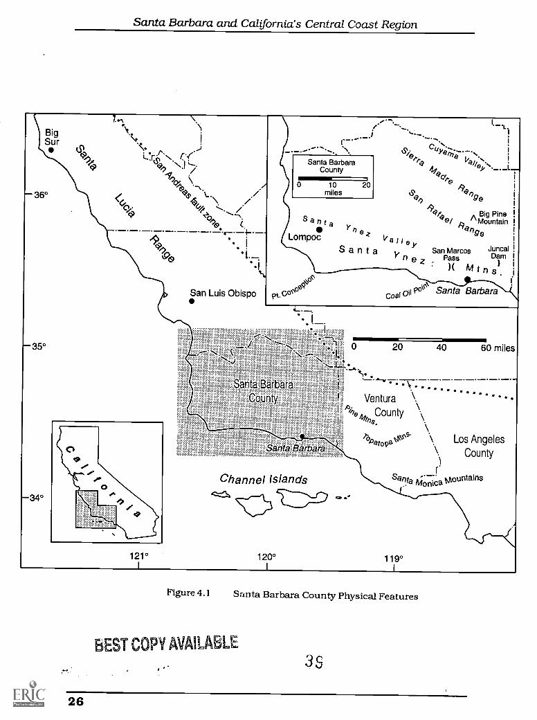
Santa Barbara and California's Central Coast Region
BigSur
(9
c90 .NI s"-./9
aed \./0 -N.
<9 /'fie
I
L
36°
350
34°
San Luis Obispo
0
121°
..Santa Barbara
County==i0 10 20
miles
SantaY
Lompoc valleySanta
---....._. I
jc
t.S'A., t/Je;;0
a fr_ .....%c'tr ot/e.k_. J.
pk.0
vnez
Coal Oil C:1(5
470cy
9afa
dela
Big Pine,, A Mountaintran
90
San Marcos JuncalPass Dam
)( M t 81.
Santa Barbara
`--
i.,
Santa Barbara
County
.1.1.
Santa Barbara
Channel Islandsdrz,
120°
0 20 40 60 miles
7; \ ...Ventura
P4)0, County \
16Datopaki'"9. \
_r-Santa Monica mountains
Los Angeles
County
119°
Figure 4.1 Santa Barbara County Physical Features
BEST COPY AVAILABLE3S
26
Images and Encounters
Even though maximum elevations in the region are not spectacularlyhigh, the terrain isfrequently very rugged. As a result, a number of isolated, roadless areas lie within shortdistances of significant population centers and heavily traveled roadways. The SantaLucias, for example, are crossed by only one minor road in a distance of around 175kilometers (110 miles). Similarly, only one road heads north out of Santa Barbara andVentura counties between Highway 101 and Interstate 5 (see Figure 7.1).
All of the Transverse and southern Coast Range provinces are west of the San Andreasfault zone. The region lies on the Pacific Plate and is being rafted northward as that platemoves past the North American Plate (see Figure 5.1). The ruggedness of the terrain, in part,is a result of the uplift of the current mountain ranges and is very recent in geologic time.All of the tectonic activity that produced the ranges in both provinces has occurred in thelast five million years (Pliocene and Pleistocene Epochs).
The entire geologic history of the area is quite short. The oldest rocks are from theFranciscan formation of the late Jurassic to late Cretaceous Periods (roughly 150 to 75million years ago). This formation is prominent in the Coast Ranges, but its origin was amystery before the development of the theory of plate tectonics. It is a complex melangeofsedimentary and volcanic rocks, all apparently deposited in deep ocean environments. Itis now thought that this formation originated in a subduction zone produced as the PacificPlate collided with and dove beneath the North American Plateapparently the same eventas the Nevadan Orogeny that produced the granitic rocks of the Sierra Nevada and theoriginal Nevadan mountains on the site of the present-day Sierra Nevada.
The rocks that make up the western Transverse Ranges are mainly from the Eocene,Oligocene, and Miocene Epochs (53.5 million to five million years ago). Most are marinesandstones and shales indicating that the area remained beneath the sea for most of thisperiod. For example, the sequence in the Santa Ynez Mountains north of Santa Barbaraincludes the Juncal and Matilij a sandstones, the Cozy Dell Shale, and the Coldwatersandstone from the Eocene Epoch (53.5 million to 39 million years ago). The one major non-marine formation is the Sespe, which consists of floodplain deposits and is Oligocene in age(39 million to 23.5 million years ago). This formation is absent in the western Santa Ynezwhere the marine rocks continue throughout the Oligocene, indicating that the coastlineran through the region somewhere.
By the beginning of the Miocene Epoch (23.5 million years ago) the sea had re-advancedover the whole region. The Rincon Shale is the main formation of the early Miocene. Thisformation weathers into unstable clay soils that are prone to sliding and tend to swell andshrink substantially as moisture is added and removed. A number of Santa Barbaraneighborhoods, particularly in the foothill areas, are built on these soils and haveexperienced significant structural problems as a result.
During the middle of the Miocene (15 to ten million years ago) deep marine basins formedthroughout what is now coastal California between San Francisco and Orange County.These basins apparently resembled current features in the Gulf of California which is beingsplit open by the spreading zone associated with the East Pacific Rise. It is thought,therefore, that the appearance of the basins may have signaled the passage of the area overthe spreading zone. This is also about the time the San Andreas fault became active in thispart of California, suggesting a shift in relative plate movements from the collision thatproduced the earlier subduction features to the shearing tangential movements associatedwith the modern San Andreas transform fault. The rocks formed in these basins (the shalesof Monterey Formation) are composed largely of organic material, rather than terrestrialsediments. Much of the material is silica derived from diatoms, which are microscopicphytoplankton. The Monterey Formation is usually finely bedded and is exposed in manyof the coastal bluffs in the Santa Barbara area.
4027
Santa Barbara and California's Central Coast Region
The uplift that began during the Pliocene Epoch (five million to 1.8 million years ago)elevated the present mountain ranges in the area. The Santa YnezMountains were lifted bya combination of folding and faulting along the Santa Ynez fault just north of the crest of therange. The structure of the range does not follow the rock strata, which have been tilted 90°or more and which cross the crest of the ridge tangentially. As a result, one moves throughsuccessively older strata going north through San Marcos Pass. At the base of the mountainsmarine conditions persisted into the Pleistocene (1.8 to million to 10,000years ago) as theyoungest rock, the Santa Barbara Formation, was formed. The coastal plain probablyemerged from the sea less than one million years ago. Frequent earthquakes andsubstantial deformation of recent alluvial depositsare compelling reminders that the upliftis continuing.
Considerable attention has been given to the cause of the east-west trend of theTransverse Ranges. The San Andreas fault, which forms the northern boundary of theprovince from Ventura County to San Bernardino County, deviates from its typicalnorthwest-southeast trend to parallel the Transverse Ranges (see Figure 5.1). No generallyaccepted explanation can account for the bend, but it clearly creates strong compressiveforces as the land west of the fault pushes against the westward bend in the fault. Evidencefrom paleomagnetic research studies in the University of CaliforniaSanta Barbara's GeologyDepartment suggest that the Transverse Ranges west of the San Andreas fault rotatedclockwise 60° to 80° between 16 and six million years ago, possibly caused by shearing alongthe Pacific-North American plate boundary. This does not explain why the east-west trendcontinues through the San Bernardino Mountains, which are east of the San Andreas fault.
Petroleum has long been exploited in the area. The local Chumash in pre-contact timesused tar from natural seeps to seal their boats. A number of natural seeps are still active,particularly offshore from Coal Oil Point just west of the University of California SantaBarbara (UCSB), and small blobs of tar are a common fixture on many local beaches. TheTransverse Ranges have been a fertile area for oil and gas exploration since thenineteenthcentury. Major discoveries were made around the end of the last century in Ventura and theSanta Barbara Channel. The latter was the first offshore field developed in the United Stateswhen it opened in 1896. It also gained considerable notoriety when a well blew out in 1969and produced the first major offshore oil spill in the United States.
ClimateThe climate of all of coastal California is Mediterranean, with a strong alternation inprecipitation between dry summers and wet winters. More than 90 percent of the annualprecipitation falls in the November-April period. Amounts generally increase northward,with San Diego averaging about 25 cm (10 inches), Los Angeles 40 cm (15 inches), SantaBarbara 45 cm (18 inches), San Luis Obispo 55 cm (22 inches), and Big Sur State Park 100cm (40 inches). This large scale trend is strongly modified by topography. Almost allprecipitation is produced by large-scale mid-latitude storms moving of the Pacific, so west-and south-facing slopes are relatively wet, as average precipitation generally increases withelevation. Leeward slopes and interior valleys show strong rainshadow effects. In SantaBarbara County, for example, precipitation rises from 45 cm (18 inches) at sea level to 75 cm(29.5 inches) at 670 meters (2,200 feet) on San Marcos Pass to 92 cm (36 inches) at 1,900meters (6,300 feet) on West Big Pine Mountain. Meanwhile Lompoc in the Santa Ynez Valleyaverages 36 cm (14 inches) and the Cuyama Valley in the interior of northern Santa BarbaraCounty (the Cuyama River forms the eastern part of northern boundary of Santa Barbara)averages only 18 cm (7 inches), technically making it a desert. Snow levels typically rangefrom around 1,000 to 2,000 meters (3,281 to 6,562 ft), so most precipitation in lowland areasfalls as rain. Occasionally, unusually cold storms will produce snow almost to sea level, butonly the higher elevation regions of the San Gabriel and San Bernardino Mountainsaccumulate significant snowpack.
41
28
Images and Encounters
Coastal central and southern California and the adjacent mountain ranges haveexceptionally large interannual variability in precipitation, so averages must be interpretedwith care. At many stations rainfall totals in the wettest years are as much as ten timesgreater than in the driest years, and the range extends from one-third of the mean to morethan 2.5 times the mean. The driest and wettest winters in the 125-year Santa Barbararecord are 11.5 cm (4.5 inches) and 114.8 cm (45.2 inches). The majority of winters arerelatively thy with around 60 percent falling below the average, but occasional winters canbe exceptionally wet. These wet winters are almost always characterized by a period ofseveral weeks of persistent heavy rains produced by a sequence of very large warm, wetstorms moving in from the southwest. Often associated with El Nino conditions in theequatorial Pacific, the link is not entirely consistent and the mechanisms are not fullyunderstood. Rainfall totals can be very high, especially on south-facing slopes at middle andhigh elevations. In January 1969, Santa Barbara received 51 cm (15.5 inches), while 92.7cm (36.5 inches) fell at San Marcos Pass, and Juncal Dam at 630 meters (2,060 feet) in theupper Santa Ynez Valley received 112.5 cm (44.3 inches). A single storm in a 12-hour periodin January 1995, produced 20 cm (eight inches) in downtown Santa Barbara and as muchas 50 cm (20 inches) in the higher elevations. Rainfall of these quantities and intensities,when combined with the steep slopes, shallow soils, and sparse vegetation covercharacteristic of the area, can produce severe flooding and landsliding problems.
In contrast to the high variability in winter rainfall, summers are remarkably uniform intheir drought. Less than 5 percent of the average annual precipitation falls between Mayand October and less than 1 percent in June, July, and August. Furthermore, only once inthe last 125 years has more than 2.5 cm (one inch) of rain fallen at Santa Barbara in Julyor August. The wettest July in 115 years at Los Angeles produced only six mm (.25 inches)of rain, and 110 have had less than one mm (.04 inches).
This persistent drought results from the North Pacific High pressure cell that movesnorth and intensifies in the summer. It produces strong subsidence and blocks thewestward penetration of moist, unstable air masses from the Gulf of Mexico and Gulf ofCalifornia, which move north out of Mexico into the interior Southwest. The strong high isalso responsible, along with the relatively cold ocean temperatures, for the temperatureinversion and coastal fog that persist throughout the summer. Air near the ocean surfaceforms a cool, moist marine layer within which fog typically forms. The marine layer is cappedby an inversion with a warmer, drier layer of subsiding air above. Since air rises only as longas it is warmer and less dense that the air around it, the inversion effectively puts a lid onthe lowest layer of the atmosphere. This phenomenon greatly exacerbates the air pollutionproblems in the region because pollutants do not disperse upward through the inversion.
Coastal fog and cold ocean water have a moderating influence on summer temperaturesat coastal stations, where average maximum temperatures are around 20°C (68°F). Thecooling influence diminishes rapidly moving away from the coast, however, and averagedaily maxima in interior valleys are 35°C (95°F) or more. This temperature differenceproduces strong sea breezes blowing inland off the ocean and typically peaking in theafternoon. The winds are very dependable and can be quite strong in areas where they areconcentrated by topography. A number of wind power farms have been established in gapsin the mountain barriers that separate coastal and desert valleys.
Winter temperatures tend to be mild in lowland areas, especially along the coast wheresub-freezing temperatures are uncommon. Interior valleys are generally colder, and low-lying areas frequently become frost pockets because of cold air drainage. Frost-sensitivecrops such as avocados are most commonly grown in coastal areas and in thermal belts onthe slopes above the colder valley floor. If air masses are sufficiently moist fog will form atnight in the valley bottoms. In most of coastal California, this radiation fog will burn offduring the day, but in the Sacramento and the San Joaquin Valleys, where it is known as
29
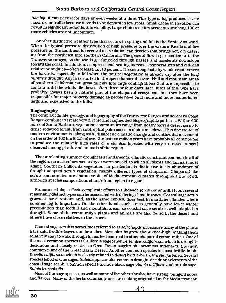
Santa Barbara and California's Central Coast Region
tole fog, it can persist for days or even weeks at a time. This type of fog produces severehazards for traffic because it tends to be densest in low spots. Small drops in elevation canresult in significant reductions in visibility. Large chain reaction accidents involving 100 ormore vehicles are not uncommon.
Another distinctive weather type that occurs in spring and fall is the Santa Ana wind.When the typical pressure distribution of high pressure over the eastern Pacific and lowpressure on the continent is reversed a circulation can develop that brings hot, dry desertair from the northeast into southern California. The general flow is perpendicular to theTransverse ranges, so the winds get funneled through passes and accelerate downslopetoward the coast. In addition, compressional heating increases temperatures and reducesrelative humiditiesoften to less than 10 percent. These strong, hot, dry winds create severefire hazards, especially in fall when the natural vegetation is already dry after the longsummer drought. Any fires started in the open chaparral-covered hill and mountain areasof southern California can grow quickly into large conflagrations that are impossible tocontain until the winds die down, often three or four days later. Fires of this type haveprobably always been a natural part of the chaparral ecosystem, but they have beenresponsible for major property damage as people have built more and more homes (oftenlarge and expensive) in the hills.
BiogeographyThe complex climate, geology, and topography of the Transverse Ranges and southern CoastRanges combine to create very diverse and fragmented biogeographic patterns. Within 200miles of Santa Barbara, vegetation communities range from nearly barren desert scrub todense redwood forest, from subtropical palm oases to alpine meadows. This diverse set ofmodern environments, along with Pleistocene climatic change and continental movementon the order of 100 km (62.5 m) over the last ten million years have probably all contributedto produce the relatively high rates of endemism (species with very restricted ranges)observed among plants and animals of the region.
The unrelenting summer drought is a fundamental climatic constraintcommon to all ofthe region, no matter how wet or dry or warm or cold, to which all plants and animals mustadapt. Southern California vegetation, in particular, is distinctive in its abundance ofdrought-adapted scrub vegetation, mainly different types of chaparral. Chaparral-likescrub communities are characteristic of Mediterranean climates throughout the world,although species compositions change from region to region.
Pronounced slope effects complicate efforts to subdivide scrub communities, but severalreasonably distinct types can be associated with differing climatic zones. Coastal sage scrubgrows at low elevations and, as the name implies, does best in maritime climates wheresummer fog is important. On the other hand, such areas generally have lower winterprecipitation than foothill and mountain areas, so coastal sage scrub is well adapted todrought. Some of the community's plants and animals are also found in the desert andothers have close relatives in the desert.
Coastal sage scrub is sometimes referred to as soft chaparral because many of the plantshave soft, flexible leaves and branches. Most shrubs grow about knee-high, making themrelatively easy to walk through in marked contrast to other chaparral communities. One ofthe most common species is California sagebrush, Artemisia calgOrnica, which is drought-deciduous and closely related to Great Basin sagebrush, Artemisia tridentata, the mostcommon plant of the Great Basin Desert. Another common species is coast brittle-bush.Encelia calYbrnica, which is closely related to desert brittle-bush, Enceliafarinosa. Severalspecies (spp.) of true sages, Salvia spp., are also common drought-deciduous elements of thecoastal sage scrub. Common species include black sage, Salvia millifera, and purple sage,Salvia leucophylla.
Most of the sage species, as well as some of the other shrubs, have strong, pungent odorsand flavors. Many of the herbs commonly used in cooking originated in the Mediterranean
4i30
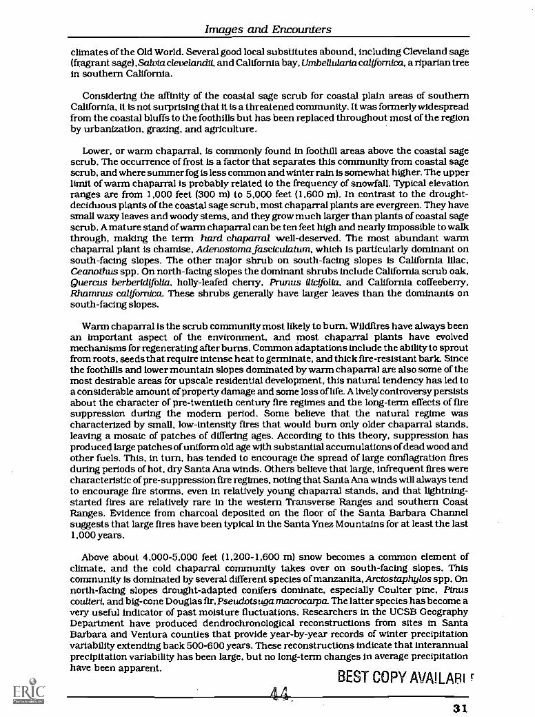
Images and Encounters
climates of the Old World. Several good local substitutes abound, including Cleveland sage(fragrant sage),Salvia cleuelandii, and California bay, Umbellularia caltfornica, a riparian treein southern California.
Considering the affinity of the coastal sage scrub for coastal plain areas of southernCalifornia, it is not surprising that it is a threatened community. It was formerly widespreadfrom the coastal bluffs to the foothills but has been replaced throughout most of the regionby urbanization, grazing, and agriculture.
Lower, or warm chaparral, is commonly found in foothill areas above the coastal sagescrub. The occurrence of frost is a factor that separates this community from coastal sagescrub, and where summer fog is less common and winter rain is somewhat higher. The upperlimit of warm chaparral is probably related to the frequency of snowfall. Typical elevationranges are from 1,000 feet (300 m) to 5,000 feet (1,600 m). In contrast to the drought-deciduous plants of the coastal sage scrub, most chaparral plants are evergreen. They havesmall waxy leaves and woody stems, and they grow much larger than plants of coastal sagescrub. A mature stand of warm chaparral can be ten feet high and nearly impossible to walkthrough, making the term hard chaparral well-deserved. The most abundant warmchaparral plant is chamise, Adenostoma fasciculatum, which is particularly dominant onsouth-facing slopes. The other major shrub on south-facing slopes is California lilac,Ceanothus spp. On north-facing slopes the dominant shrubs include California scrub oak,Quercus berberidifolia, holly-leafed cherry, Prunus ilicfolia, and California coffeeberry,Rhamnus californica. These shrubs generally have larger leaves than the dominants onsouth-facing slopes.
Warm chaparral is the scrub community most likely to burn. Wildfires have always beenan important aspect of the environment, and most chaparral plants have evolvedmechanisms for regenerating after burns. Common adaptations include the ability to sproutfrom roots, seeds that require intense heat to germinate, and thick fire-resistant bark. Sincethe foothills and lower mountain slopes dominated by warm chaparral are also some of themost desirable areas for upscale residential development, this natural tendency has led toa considerable amount of property damage and some loss of life. A lively controversy persistsabout the character of pre-twentieth century fire regimes and the long-term effects of firesuppression during the modern period. Some believe that the natural regime wascharacterized by small, low-intensity fires that would burn only older chaparral stands,leaving a mosaic of patches of differing ages. According to this theory, suppression hasproduced large patches of uniform old age with substantial accumulations of dead wood andother fuels. This, in turn, has tended to encourage the spread of large conflagration firesduring periods of hot, dry Santa Ana winds. Others believe that large, infrequent fires werecharacteristic of pre-suppression fire regimes, noting that Santa Ana winds will always tendto encourage fire storms, even in relatively young chaparral stands, and that lightning-started fires are relatively rare in the western Transverse Ranges and southern CoastRanges. Evidence from charcoal deposited on the floor of the Santa Barbara Channelsuggests that large fires have been typical in the Santa Ynez Mountains for at least the last1,000 years.
Above about 4,000-5,000 feet (1,200-1,600 m) snow becomes a common element ofclimate, and the cold chaparral community takes over on south-facing slopes. Thiscommunity is dominated by several different species of manzanita, Arctostaphylos spp. Onnorth-facing slopes drought-adapted conifers dominate, especially Coulter pine, Puntscoulteri, and big-cone Douglas fir, Pseudotsuga rnacroccupa. The latter species has become avery useful indicator of past moisture fluctuations. Researchers in the UCSB GeographyDepartment have produced dendrochronological reconstructions from sites in SantaBarbara and Ventura counties that provide year-by-year records of winter precipitationvariability extending back 500-600 years. These reconstructions indicate that interannualprecipitation variability has been large, but no long-term changes in average precipitationhave been apparent.
BEST COPY AVAILARI r
4.431
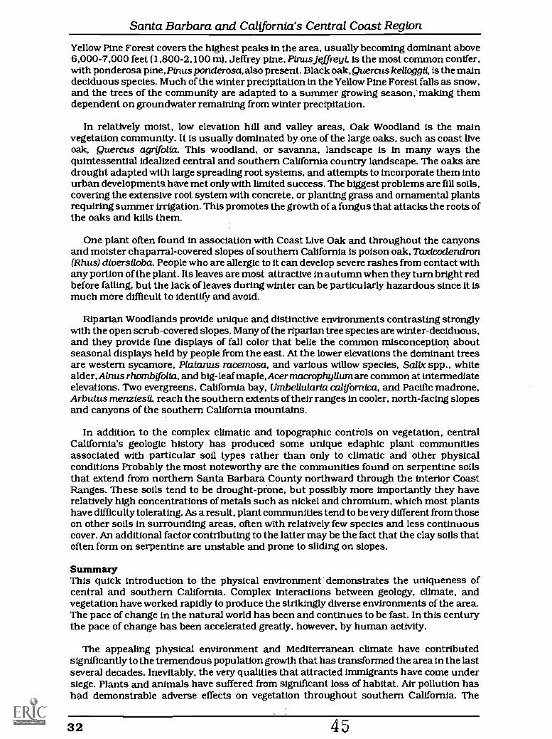
Santa Barbara and California's Central Coast Region
Yellow Pine Forest covers the highest peaks in the area, usually becoming dominant above6,000-7,000 feet (1,800-2,100 m). Jeffrey pine, Pinta jeffreyi, is the most common conifer,with ponderosa pine, Pinus ponderosa, also present. Black oak, Quercus kelloggii, is the maindeciduous species. Much of the winter precipitation in the Yellow Pine Forest falls as snow,and the trees of the community are adapted to a summer growing season; making themdependent on groundwater remaining from winter precipitation.
In relatively moist, low elevation hill and valley areas, Oak Woodland is the mainvegetation community. It is usually dominated by one of the large oaks, such as coast liveoak, Quercus agrifolia. This woodland, or savanna, landscape is in many ways thequintessential idealized central and southern California country landscape. The oaks aredrought adapted with large spreading root systems, and attempts to incorporate them intourban developments have met only with limited success. The biggest problems are fill soils,covering the extensive root system with concrete, or planting grass and ornamental plantsrequiring summer irrigation. This promotes the growth of a fungus that attacks the roots ofthe oaks and kills them.
One plant often found in association with Coast Live Oak and throughout the canyonsand moister chaparral-covered slopes of southern California is poison oak, Taxicodendron(Rhus) diuersiloba. People who are allergic to it can develop severe rashes from contact withany portion of the plant. Its leaves are most attractive in autumn when they turn bright redbefore falling, but the lack of leaves during winter can be particularly hazardous since it ismuch more difficult to identify and avoid.
Riparian Woodlands provide unique and distinctive environments contrasting stronglywith the open scrub-covered slopes. Many of the riparian tree species are winter-deciduous,and they provide fine displays of fall color that belie the common misconception aboutseasonal displays held by people from the east. At the lower elevations the dominant treesare western sycamore, Platanus racemosa, and various willow species, Salix spp., whitealder, Alnus rhombYblia, and big-leaf maple,Acer macrophyllum are common at intermediateelevations. Two evergreens, California bay, Umbellularta calYbrnica, and Pacific madrone,Arbutus menziesti, reach the southern extents of their ranges in cooler, north-facing slopesand canyons of the southern California mountains.
In addition to the complex climatic and topographic controls on vegetation, centralCalifornia's geologic history has produced some unique edaphic plant communitiesassociated with particular soil types rather than only to climatic and other physicalconditions Probably the most noteworthy are the communities found on serpentine soilsthat extend from northern Santa Barbara County northward through the interior CoastRanges. These soils tend to be drought-pione, but possibly more importantly they haverelatively high concentrations of metals such as nickel and chromium, which most plantshave difficulty tolerating. As a result, plant communities tend to be very different from thoseon other soils in surrounding areas, often with relatively few species and less continuouscover. An additional factor contributing to the latter may be the fact that the clay soils thatoften form on serpentine are unstable and prone to sliding on slopes.
SummaryThis quick introduction to the physical environment demonstrates the uniqueness ofcentral and southern California. Complex interactions between geology, climate, andvegetation have worked rapidly to produce the strikingly diverse environments of the area.The pace of change in the natural world has been and continues to be fast. In this centurythe pace of change has been accelerated greatly, however, by human activity.
The appealing physical environment and Mediterranean climate have contributedsignificantly to the tremendous population growth that has transformed the area in the lastseveral decades. Inevitably, the very qualities that attracted immigrants have come undersiege. Plants and animals have suffered from significant loss of habitat. Air pollution hashad demonstrable adverse effects on vegetation throughout southern California. The
32 45
Images and Encounters
California condor no longer exists in the wild. Coastal sage scrub is nearly gone, as are someof its animal inhabitants
On the other hand, substantial areas remain that have not been overdeveloped where theeffects of modern society, although not absent, are not overwhelming. Much has been lost,but much remains, providing hope and a challenge for future generations to do a better jobof maintaining the beauty and living with the hazards of the natural environment.
33
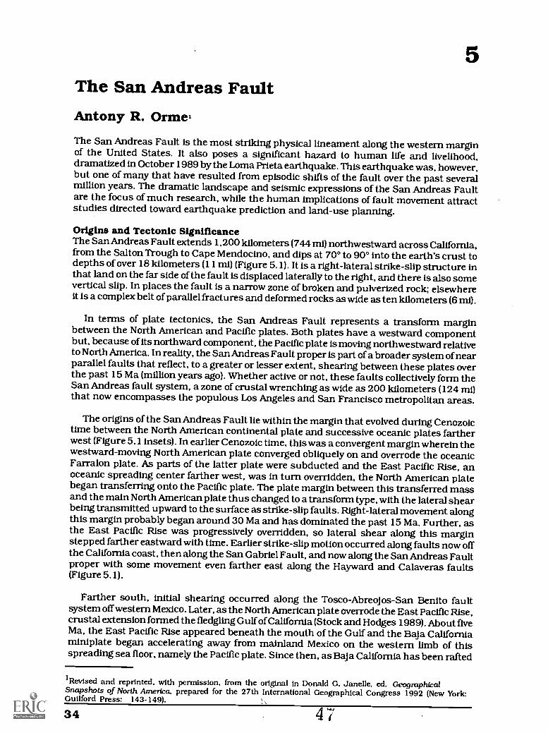
5The San Andreas FaultAntony R. Orme.
The San Andreas Fault is the most striking physical lineament along the western marginof the United States. It also poses a significant hazard to human life and livelihood,dramatized in October 1989 by the Loma Prieta earthquake. This earthquake was, however,but one of many that have resulted from episodic shifts of the fault over the past severalmillion years. The dramatic landscape and seismic expressions of the San Andreas Faultare the focus of much research, while the human implications of fault movement attractstudies directed toward earthquake prediction and land-use planning.
Origins and Tectonic SignificanceThe San Andreas Fault extends 1,200 kilometers (744 mi)northwestward across California,from the Salton Trough to Cape Mendocino, and dips at 70° to 90° into the earth's crust todepths of over 18 kilometers (11 mi) (Figure 5.1). It is a right-lateral strike-slip structure inthat land on the far side of the fault is displaced laterally to the right, and there is also somevertical slip. In places the fault is a narrow zone of broken and pulverized rock; elsewhereit is a complex belt of parallel fractures and deformed rocks as wide as ten kilometers (6 mi).
In terms of plate tectonics, the San Andreas Fault represents a transform marginbetween the North American and Pacific plates. Both plates have a westward componentbut, because of its northward component, the Pacific plate is moving northwestward relativeto North America. In reality, the San Andreas Fault proper is part of a broader system of nearparallel faults that reflect, to a greater or lesser extent, shearing between these plates overthe past 15 Ma (million years ago). Whether active or not, these faults collectively form theSan Andreas fault system, a zone of crustal wrenching as wide as 200 kilometers (124 mi)that now encompasses the populous Los Angeles and San Francisco metropolitan areas.
The origins of the San Andreas Fault lie within the margin that evolved during Cenozoictime between the North American continental plate and successive oceanic plates fartherwest (Figure 5.1 insets). In earlier Cenozoic time, this was a convergent margin wherein thewestward-moving North American plate converged obliquely on and overrode the oceanicFarralon plate. As parts of the latter plate were subducted and the East Pacific Rise, anoceanic spreading center farther west, was in turn overridden, the North American platebegan transferring onto the Pacific plate. The plate margin between this transferred massand the main North American plate thus changed to a transform type, with the lateral shearbeing transmitted upward to the surface as strike-slip faults. Right-lateral movement alongthis margin probably began around 30 Ma and has dominated the past 15 Ma. Further, asthe East Pacific Rise was progressively overridden, so lateral shear along this marginstepped farther eastward with time. Earlier strike-slip motion occurred along faults now offthe California coast, then along the San Gabriel Fault, and now along the San Andreas Faultproper with some movement even farther east along the Hayward and Calaveras faults(Figure 5.1).
Farther south, initial shearing occurred along the Tosco-Abreojos-San Benito faultsystem off western Mexico. Later, as the North American plate overrode the East Pacific Rise,crustal extension formed the fledgling Gulf of California (Stock and Hodges 1989). About fiveMa, the East Pacific Rise appeared beneath the mouth of the Gulfand the Baja Californiaminiplate began accelerating away from mainland Mexico on the western limb of thisspreading sea floor, namely the Pacific plate. Since then, as Baja California has been rafted
1Revised and reprinted, with permission, from the original in Donald G. Janelle, ed. GeographicalSnapshots of North America prepared for the 27th International Geographical Congress 1992 (New York:Guilford Press: 143-149).
34 4 7
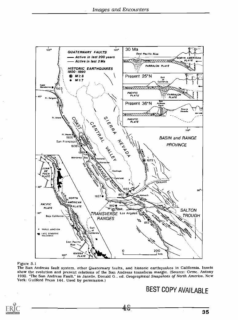
Images and Encounters
125° 120°QUA TERNARY FAULTS
Active in last 200 yearsActive in last 2Ma
CopeMendacinoC
HISTORIC EARTHQUAKES1800-1990tój M? 8
M?7
1 %..
Pt. Delgada
PLATE
Present 25°N
PACIFICPLATE
71.
Pt. Arena
0 PACIFIC.. PLATE0 .'. CC\
13 115°.." %
BASIN and RANGE.. ,c(' V.\ PROVINCE
. c":. . 0Monterey Holliste;.. N:i.
In -PInnaclis;:...
%I....Coalinga
.
. \
Pt. Reyes
1906
San Francisco
1838
SierraNevada 4
o°
JUAN .0DE
FUCAPLATE
field
1952 N,1857 C) Neenach
PACIFICPLATE
o°Baja California
tNORTHAMERICAN
PLATE
0 TRIPLE JUNCTION
LATE CENOZOICVOLCANICS
1927,
18120
TRANSVERSE Los Angele(4.o
RANGES1812 o'
", Gulfof
,sCalifornia
35°
SALTON*. . TROUGH
East PacificAlso
120°RIVERA
PLATE
0I 1km
Figure 5.1The San Andreas fault system, other Quaternary faults, and historic earthquakes in California. Insetsshow the evolution and present relations of the San Andreas transform margin. (Source: Orme, Antony1992. "The San Andreas Fault," in Janelle, Donald G., ed. Geographical Snapshots of North America. NewYork: Guilford Press 144. Used by permission.)
BEST COPY AVAILABLE
.0
35
Santa Barbara and California's Central Coast Region
northwestward at a mean rate of 56 to 60 millimeters (2.24 to 2.4 in) per year (Larson 1972;Minster and Jordan 1987), transform faults offsetting the East Pacific Rise within the Gulfhave propagated northward into the continental crust of the Salton Trough, formingsequential right-lateral strike-slip faults of which the San Andreas is currently the mostprominent. Furthermore, as the Baja California miniplate collided with the resistant rootsof the Sierra Nevada, compression formed the Big Bend in the San Andreas Fault andseverely buckled the Pacific Coast (Orme 1980). North of Cape Mendocino, these evolvingplate relations remain at an earlier stage as fragments of the Farralon plate, namely theGorda and Juan de Fuca plates, continue to be subducted beneath the North Americanplate, with associated volcanism in the Cascade Range farther east.
Surface ExpressionThe path of the San Andreas Fault across California may be divided into three segments. Inthe south, through the Salton Trough, a 50-kilometer- (31 mi-) wide fault zone trends N45°Wfor 300 kilometers (186 mi) and comprises several active faults that converge on the CajonPass. For 180 kilometers (112) mi from the Cajon Pass, the Big Bend of the San Andreas Faulttrends N75°W as a narrow lineament north of the Transverse Ranges. The fault then trendsN35°W over the remaining 720 kilometers (447 mi) to Cape Mendocino, crosses the coast justsouth of San Francisco, and passes east of the Point Reyes Peninsula and Point Arena toPoint Delgada before turning west into the Mendocino fracture zone.
Because of intense deformation and recurrent fracturing or persistent creep, rocks alongthe fault are relatively soft and easily eroded. Thus, where the fault zone is narrow, its courseis marked by a linear trough characterized by fault scarps, pressure ridges, and sag ponds.Repeated displacement along the fault is well shown by offset streams and dislocated alluvialfans, notably in the Carrizo Plain and Transverse Ranges. Fault-controlled groundwaterbarriers commonly lead to springs and surface seepage. Local compression often causesuplift within the fault zone, as in the Ocotillo badlands in the Salton Trough. Mountain frontsalongside the fault are markedly linear with numerous truncated spurs. Duringearthquakes, liquefaction at depth may cause sand boils or mud volcanoes at the surface aswater-saturated sediments flow upward along fractures. Continuing geothermal andvolcanic activity within the fault zone, as in the Salton Trough where five rhyolite domes haveextruded onto Quaternary sediments, have led to the plate margin's designation as a "leakytransform" boundary.
At a regional scale, compression of the Pacific plate against the roots of the NorthAmerican plate has forced excess mass upward to form prominent mountains, notably theTransverse Ranges, which rose rapidly when the transform boundary collided with theSierra Nevada and created the Big Bend in the San Andreas Fault. As these mountainsrotated to their present east-west alignment and continuing compression triggered thrustfaulting, marginal pull-apart structures such as the Los Angeles and Santa Maria basinsalso formed. The 260-kilometer (161 mi) left-lateral Garlock Fault may have been created byrelated displacement southeast of the Sierra Nevada. Farther north, the Coast Ranges arebeing compressed by active thrusting along their eastern margins (Wentworth and Zoback1989). Lateral displacement of regional drainage is illustrated by the San Benito River whichflows northwest for 100 kilometers (63 mi) along the San Andreas fault zone before breakingseaward to Monterey Bay.
Fault Movement and Plate DisplacementBecause plate displacement along the San Andreas Fault is usually associated withearthquakes, an understanding of slip rates along the fault is important, particularly asrecent movement may be the best clue to future fault behavior and earthquake prediction.Displacement along the fault may be deduced from a variety of temporal evidence. Long-termdisplacement is indicated, for example, by early Miocene volcanic rocks at the Pinnacles andNeenach (west central California), which originated from a common eruptive center around23 Ma and have since been separated by 310 kilometers (192 mi) of movement along the SanAndreas Fault (Matthews 1976). Marine sediments beneath the southern. Central Valley and
364
Images and Encounters
the Santa Cruz Mountains have been similarly offset by 325 kilometers (202 mi) sinceearlyMiocene times (Stanley 1987). Geologic discordances across the Gulf of California indicatethat Baja California has been rafted a similar distance northwest away from mainlandMexico during this interval. Although initial Miocene slip rates were as low as threemillimeters (.12 in) per year, most evidence indicates a long-term slip rate of 13 to 14millimeters (.52 to .56 in) per year over the past 23 million years. Such rates have not,however, been constant in time or space. For example, Colorado River deposits on thewestern margins of the SaltonTrough have been displaced 130 kilometers (81 mi) from theirsource over the past 2.8 Ma, for a rate of 46 millimeters (1.84 in) per year (Winker and Kidwell1986).
Medium-term displacement is indicated at Wallace Creek, in the Carrizo Plain, whichhas been offset 128 meters (420 ft) along the San Andreas Fault over the past 3,680 yearsfor a mean slip rate of 35 millimeters (1.4 in) per year (Sieh and Jahns 1984). Nearbyalluvial-fan deposits have been offset 475 meters (1,558 ft) over 13,250 years for a mean sliprate of 36 millimeters (1.44 in) per year. Near the Cajon Pass, dislocated alluvial depositsindicate a slip rate of 25 millimeters (1 in) per year over the past 14,400 years which, whenadded to slip of ten millimeters (.40 in) per year on the San Jacinto Fault, is comparable tothe Wallace Creek data (Weldon and Sieh 1985). Late Quaternary slippage in the SaltonTrough approximates 23 to 35 millimeters (.92 to 1.4 in) per year (Keller et al. 1982).
For the past 100 years, short-term slip rates of 32 to 36 millimeters (1.28 to 1.44 in) peryear have been revealed between Parkfield and San Francisco Bay by periodic geodeticobservations (for example, Prescott et al. 1981), augmented since 1985 by monthlyobservations of relative vectors using the Global Positioning System of survey satellites. TheFarralon Islands on the Pacific plate 30 kilometers (19 mi) west of San Francisco are shiftingnorthwards at this rate relative to fixed points east of the San Andreas Fault.
The medium- and short-term measurements together suggest a mean slip rate of 34millimeters (1.4) per year for Holocene times. This is an order of magnitude greater than theinferred Miocene rate of three millimeters (.12 in) per year and larger than the long-termrate of 13 to 14 millimeters (.52 to .56 in) per year. Movement along the San Andreas Faulthas thus accelerated in the recent geologic past and may be greater now than at any timeover the past 30 Ma.
Magnetic anomalies and plate reconstructions across the Gulf of California indicate,however, plate separation of 56 to 60 millimeters (2.24 to 2.4 in) per year over the past fourMa (Larson 1972; Minster and Jordan 1987). To explain this discrepancy between platedisplacement of 56 to 60 millimeters (2.24 to 2.4 in) per year and a San Andreas slip rateof 34 millimeters (1.4 in) per year, it is necessary to abandon rigid-plate concepts in favorof more deformable models and to invoke right-lateral motion of eight to 27 millimeters (.32to 1.08 in) per year on faults to the west and the extension of the Basin and Range Provinceto the east by ten to 20 millimeters (.40 to .80 in) per year. These scenarios are wellsupported by evidence for slip along the 420-kilometer (260 mi-) San Gregorio-Hosgri faultsystem offshore, which may have been displaced 100 kilometers (62 mi) since Miocenetimes, and by normal faulting east of the Sierra Nevada, which gave rise, among others, tothe great M8 Owens Valley earthquake of 1872. In the Santa Cruz Mountains, the SanAndreas Fault accounts for only 13 millimeters (.52 in) per year of relative plate motion; theremainder is distributed east and west, along the Hayward-Calaveras and San Gregoriofault systems respectively.
Earthquake History and PredictionCalifornia has a historic record of earthquake activity extending back for more than 200years and mounting evidence is becoming available for datable prehistoric events. In 1769,the Portola expedition felt 24 earthquakes in one week as it crossed the Los Angeles basin.Franciscan missionaries, soldiers, and early newspapers later documented nineteenthcentury events but such records were inevitably incomplete, confined as they were toearthquakes actually felt in inhabited areas and uncertain as to which fault had moved.
56 37
Santa Barbara and California's Central Coast Region
The first permanent earthquake laboratories were established by the University ofCalifornia in 1887 and statewide seismographiccoverage existed by 1932. Based in part onearlier systems, the modified Mercalli scale (MM) of earthquake intensities, which ranksshaking in ascending order from MMI to MMVII, was defined in 1931, and the open-endedlogarithmic scale of earthquake magnitude (M) was introduced by Charles Richter of theCalifornia Institute of Technology in 1935. Since then, both scales have been used todescribe earthquakes and retrofitted, as far as possible, to past events.
Since 1800, California has experienced more than 70 earthquakes ofM6 or larger,including ten over M7, of which three exceeded M8 (Figure 5). Of these, half have occurredalong the San Andreas Fault proper, including the M8+ Fort Tejon earthquake of 1857 andthe M8.3 San Francisco earthquake of 1906. The record ofsmaller butstill troubling quakesis much larger: 188 events of M4 or greater occurred in California between 1975 and 1979,again about half along the San Andreas Fault. Most such earthquakes focus at shallowdepths of less than 18 kilometers (11 mi) and the larger ones are thus particularly damagingat the surface.
In southern California, the 240-kilometer (149 mi) San Jacinto Fault is among the mostseismically-active strands of the San Andreas system, having experienced nine events ofM6 or larger since 1890. A complex freeway interchange between Interstates 10 and 15straddles this fault! The nearby Imperial Fault has also been frequentlyactive, with an M6.7event in 1940 offsetting citrus groves, whereas an M6.6 event in 1979 caused 30 kilometers(19 mi) of ground rupture with 55 centimeters (22 in) of right-lateral and 19 centimeters (7.6in) of vertical displacement. Indeed, in the pervasively faulted Salton Trough, earthquakeswarms of low to moderate intensity are quite frequent as strain is released upwardsthrough thick, poorly compacted Quaternary sediments.
The largest historic earthquake along the Big Bend segment was the M8+ Fort Tejonearthquake of 1857 when the San Andreas Fault sustained as much as 9.5 meters (32 ft)of lateral slip over the 320 kilometers (198 mi) between the Cajon Pass and Parkfield. Thefresh tectonic relief of this segment includes numerous sag ponds and fault scarpsproduced during this event. Intensities of MMVII or larger were felt from Los Angeles toMonterey but, owing to the then-sparse population, damage was small (an MMVII eventcauses people to run outdoors, and damage to poorly built structures is considerable). Since1857 this fault segment has remained locked, suggesting that stresses accumulate hereover long periods until relieved during a great earthquakethe "big one" anticipated bysouthern California residents.
North of the Big Bend, tectonic creep increases to 32 to 36 millimeters (1.28 to 1.44 in)per year along the San Andreas Fault as it passes through the Carrizo Plain to Parkfield,and then diminishes farther north toward Monterey Bay, but is found along the Hayward-Calaveras system past Hollister. Creep may reflect the nature of basement rocks andstructures. Because tectonic creep inhibits the accumulation of strain energy, which wouldotherwise be released by larger earthquakes, this fault segment has experienced mostly lowto moderate events, notably the Parkfield earthquakes of 1932 (M6) and 1966 (M5.5). Thiscreeping segment attracts scientific attention because periodic measurements of strainand creep may provide early detection of altered conditions preceding an earthquake.
The San Francisco region has suffered several moderate to large historic earthquakeswithin the San Andreas system. An M7 event caused 40 kilometers (25 mi) of surfaceruptures along the main fault near San Francisco in 1838, whereasacross San FranciscoBay two M6.8 events occurred on the Hayward Fault in 1836 and 1868. The great M8.3earthquake of April 1906 ruptured along 450 kilometers (279 mi) of the San Andreas Faultfrom near Monterey By northwest to beyond Point Delgada, with up to five meters (17 ft)of right-lateral slip in the trough east of the Point Reyes peninsula. Thisevent raised studiesof the San Andreas Fault to a higher plane (Lawson et aL 1908). Furthermore, realizationthat displacement died out within 30 kilometers (19m1) east and west of the fault led to thetheory of elastic rebound, which states that crustal rocks that are progressively strained
38
Images and Encounters
by slow plate movement are returned to an unstrained state by the sudden faultdisplacements that cause earthquakes.
More recently, the M7.1 Loma Prieta earthquake of October 1989, whose epicenter lay inthe Santa Cruz Mountains 100 kilometers (62 mi) south of San Francisco, was caused bycompressive slip along a 40-kilometer (25 mi-) segment of the San Andreas Fault thatruptured the crust from a depth of 18 kilometers (11 mi) to within five kilometers (3.1 mi) ofthe surface. Between 1906 and 1989, this fault segment had remained relatively quiet, oraseismic, and a 30 percent chance of an M7 earthquake had been predicted for the period1988 to 2018! Displacement on the 70° fault plane amounted to two meters (7 ft) laterally and1.3 meters (4.3 ft) vertically, but little primary surface faulting occurred (Pla fker andGalloway 1989). Instead, ten seconds of seismic shaking at depth caused extensive surfacecracking and many landslides, while liquefaction of water-saturated sediments andartificial fills caused much damage around San Francisco and Monterey Bays. Intensitiesof MMVII or larger were felt from Salinas in the south to Berkeley in the north. Theearthquake caused sixty-seven known deaths, more than $6 billion in property damage, thecollapse of several bridge and freeway structures, and left more than 12 thousand peoplehomeless. Some fifty-one aftershocks of M3 or larger occurred within twenty-four hours ofthe main shock. Despite this event, the probability of another M7 earthquake within the SanAndreas fault system around San Francisco Bay remains high. There have also beenfrequent earthquakes at the far north end of the San Andreas Fault, notably the M7.2 eventnear Cape Mendocino in 1923. This area is a triple junction where the North American,Pacific, and Gorda plates meet.
Society is, of course, less concerned about past earthquakes than future events, andmuch scientific effort is now directed toward forecasting more precisely the time, place, andsize of future shocks. Several avenues of inquiry are available for earthquake prediction butall have limitations. First, the historic record is useful in directing attention to active faultsbut is far too short for fine-tuned estimates of future earthquakes. The large 1838 and 1906earthquakes on the San Andreas Fault near San Francisco occurred 68 years apart and,although strain was known to be accumulating, the next major event came in 1989, eighty-three years later, and focused on a different fault segment. Second, where the record can beextended back into prehistoric time, earthquake recurrence is better understood but stillvague. For example, periodic fault displacement and liquefaction of radiocarbon-datedmarsh sediments at Pallett Creek, 50 kilometers (31 mi) northeast of Los Angeles, have beenattributed to nine large earthquakes between A.D. 575 and 1857 (Sieh 1978). Although anaverage recurrence interval of 160 years is suggested, the actual interval between eventsranged from 55 to 275 years! Third, slip rates may be used to infer earthquake recurrenceintervals. For example, the 9.5 meters (31 ft) of right-lateral slip sustained by the SanAndreas Fault at Wallace Creek in the 1857 earthquake suggest, when compared with themedium-term slip rate of 34 millimeters (1.36 in) per year, that the 1857 event was precededby 280 years of strain accumulation (Sieh and Jahns 1984). Variations in fault offset andother assumptions, however, indicate that the latest three recurrence intervals range from240 to 450 years! Fourth, geodetic measurements and strain-meters measure currentlyaccumulating strain with much greater precision than in the past, but earthquakeprediction remains confounded by variable crustal behavior, especially between locked andcreeping fault segments.
Finally, even where the past role and future significance of the San Andreas Fault can beevaluated, seismic prediction in California is confounded because many earthquakes occuralong other faults within the straining plate margin and some occur on previously unknownor buried faults. For example, wrenching along the Newport-Inglewood fault zone caused theM6.3 Long Beach earthquake of 1933, the severe damage that resulted led to state regulationof public school construction (Field Act 1933). An M7 event on this fault would have astronger impact on the Los Angeles metropolitan area than an M8 event on the San AndreasFault 50 kilometers (31 mi) to the northeast (Toppozadaet al. 1989). The M6.4 San Fernandoearthquake of 1971, which occurred on a largely ignored east-west thrust fault in theTransverse Ranges within that metropolitan area, caused sufficient destruction and death
BEST COPY AVAIl API 1G. 39
Santa Barbara and California's Central Coast Region
to promote statewide studies designed to restrict construction in active fault zones (Alquist-Priolo Special Studies Zones Act 1972). (A pre-dawn earthquake struck the Northridge areaof Los Angeles on 17 January 1994. It claimed 61 lives and caused widespread devastation.The main jolt lasted 30 seconds and measured M6.8. Damage was estimated at between $13and $20 billion.) The destructive M6.7 Coalinga quake of 1983 occurred close to the SanAndreas Fault but on a buried thrust fault whose existence has since led to reappraisal ofplate relations along the eastern margin of the Coast Ranges.
In short, California is earthquake country and the San Andreas Fault is the principal, butnot the only, cause of this activity. An earthquake of M7 or larger is likely to occur somewherein California every 15 to 25 years, and the Loma Prieta event of 1989 emphasized the needfor further diligence in developing and enforcing land-use policies designed to reduce theloss of life and property during future earthquakes. Scientific understanding of the physicaldimensions of faults and earthquakes has increased rapidly in recent years and, whereassociety may not yet be precisely forewarned, it must at least be prepared.
ReferencesKeller, LA., M. S. Bonkowski, R J. Korsch, and R J. Shlemon 1982. "Tectonic Geomorphology
of the San Andreas Fault Zone in the Southern Indio Hills, Coachella Valley,California." Geological Society of America Bulletin 93:46-56.
Larson, R L. 1972. "Bathymetry, Magnetic Anomalies, and Plate Tectonics History of theMouth of the Gulf of California. "Geological Society ofAmerica Bulletin 83:3345-3360.
Lawson, A. C., et al. 1908. The California Earthquake of April 18, 1906; Report of the StateEarthquake Investigation Commission. Washington: Carnegie Institution.
Matthews, V. 1976. "Correlation of Pinnacles and Neenach Volcanic Formations and TheirBearing on San Andreas Fault Problem."AmericanAssociationofPetroleum GeologistsBulletin60:2128-2141.
Minster, J. B., and T. H. Jordan. 1987. "Vector Constraints on Western U.S. Deformationfrom Space Geodesy, Neotectonics, and Plate Motions." Journal of GeophysicalResearch 92:4298-4304.
Orme, A. R. 1980. "Marine Terraces and Quaternary Tectonism, Northwest Baja California,Mexico."Physical Geography 1:138-161.
Plafker, G., and J. P. Galloway eds. 1989. "Lessons Learned from the Loma Prieta, California,Earthquake of October 17. 1989." United States Geological Survey Circular 1045.
Prescott, W. H., M. Lisowski, and J. C. Savage 1981. "Geodetic Measurements of CrustalDeformation on the San Andreas, Hayward, and Calaveras Faults near SanFrancisco, California."Journal of Geophysical Research 86:10853-10869.
Sieh, K. E. 1978. "Prehistoric Large Earthquakes Produced by Slip on the San Andreas Faultat Pallett Creek, California."Journal of Geophysical Research 83:3907-3939.
and R H. Jahns 1984. "Holocene Activity of the San Andreas Fault at Wallace Creek,California." Geological Society ofAmerica Bulletin 95:883-896.
Stanley, R G. 1987. "New Estimates of Displacement along the San Andreas Fault in CentralCalifornia Based on Paleobathymetry and Paleogeography." Geology 15:171-174.
Stock, J. M., and K. V. Hodges 1989. "Pre-Pliocene Extension around the Gulf of Californiaand the Transfer of Baja California to the Pacific Plate." Tectonics 8:99-115.
5340
Images and Encounters
Toppozada, T. R. J. H. Bennett, G. Borchardt, R Saul, and J. E. Davis 1989. "EarthquakePlanning Scenario for a Major Earthquake on the Newport-Inglewood Fault Zone."CaWornia Geology 42:75-84.
Weldon, R J., and K. E. Sieh 1985. "Holocene Rate of Slip and Tentative Recurrence Intervalfor Large Earthquakes on the San Andreas Fault, Cajon Pass, Southern California.Geological Society ofAmerica Bulletin 96:793-812.
Wentworth, C. M., and M. D. Zoback 1989. "The Style of Late Cenozoic Deformation at theEastern Front of the California Coast Ranges." Tectonics 8:237-246.
Winker, C. D., and S. M. Kidwell 1986. "Paleocurrent Evidence for Lateral Displacement ofthe Pliocene Colorado River Delta by the San Andreas Fault System, SoutheasternCalifornia." Geology 14:788-791.
41
6Santa Barbara's Water ResourcesEdited by Kate Rees,
Santa Barbara boasts a beautiful physical location, overlooking a particularly attractivesection of California coastline. Like the rest of coastal Southern California, it experiencesa Mediterranean climate with hot, dry summers, cool, wet winters, and fairly low averagerainfall. Because of these conditions and the many competing demands, water in SantaBarbara County has always been, and continues to be, a precious resource.
Surface Water HydrologyThe Santa Ynez River watershed encompasses about 900 square miles (2,331 sq km) andis located in the central part of Santa Barbara County (Figures 4.1 and 6.1). The majorityof the Santa Ynez River watershed is undeveloped and consists mostly of brushlands,rangelands, and agricultural fields. The south side of the watershed is formed by the SantaYnez Mountains. These mountains, ranging in elevation from 2,000 to 4,000 feet (610 to1,219 m), separate the Santa Ynez River watershed from the South Coast of the county. Thenorth side of the watershed is formed by the Purisima Hills and the San Rafael Mountains,which range in elevation from 4,000 to 6,000 feet (1,219 to 1,829 m).
The Santa Ynez River flows westerly about 90 miles (145 km) to the Pacific Ocean, passingthrough Jameson Lake, Gibraltar Reservoir, and Lake Cachuma. Immediately above LakeCachuma, the river passes through a narrow valley between the San Rafael and Santa YnezMountains. Below Bradbury Dam, the river passes between the Santa Ynez Mountains andthe southern edge of the Santa Ynez upland, and through the broad part of the valley nearBuellton. West of Buellton, the river flows through a narrow meandering stretch to theNarrows and emerges onto the broad, flat Lompoc Plain. The Santa Ynez River flows acrossthe Lompoc Plain for about thirteen miles (8 km) and empties into the ocean at Surf. Severalmajor tributaries downstream of Bradbury Dam contribute significant flows to the river,including Santa Agueda, Alamo Pintado, La Zaca, Alisal, Salsipuedes, and San MiguelitoCreeks.
The flow of the river has been intermittent, both in the past and under current dammedoperations. Winter flows were largely uncontrolled prior to the construction of BradburyDam, with virtually no flow in the summer months. Since operations of Bradbury Dam beganin 1953, the winter flows have been moderated by reservoir operations and previouslynonexistent summer flows have been replaced with releases for downstream water rights.
Precipitation and Runoff in the Santa Ynez River WatershedThe Santa Ynez River watershed has a Mediterranean climate with hot, dry summers andcool, wet winters. Almost all precipitation occurs between November and April, althoughlarge variations in annual quantities occur within the watershed. Annual rainfall rangesfrom about 14 inches (36 cm) near the ocean to about 30 inches (76 cm) at Juncal Dam withhigher rates in the headwater areas because of orographic effects.
The upper portion of the watershed is regulated by Juncal, Gibraltar, and Bradburydams. Juncal and Gibraltar dams are located above Bradbury Dam (Lake Cachuma), andregulate 14 and 216 square miles (36 and 560 sq km) respectively. Lake Cachuma regulatesabout 417 square miles (1,080 sq km), or less than half of the Santa Ynez River basin. Theaverage annual runoff of the Santa Ynez River at Bradbury Dam is about 71,400 acre feetper year.
1Taken from the Environmental Impact Statement-Environmental Impact Report, Cachuma Project Contract
Renewal, December 1995.
42
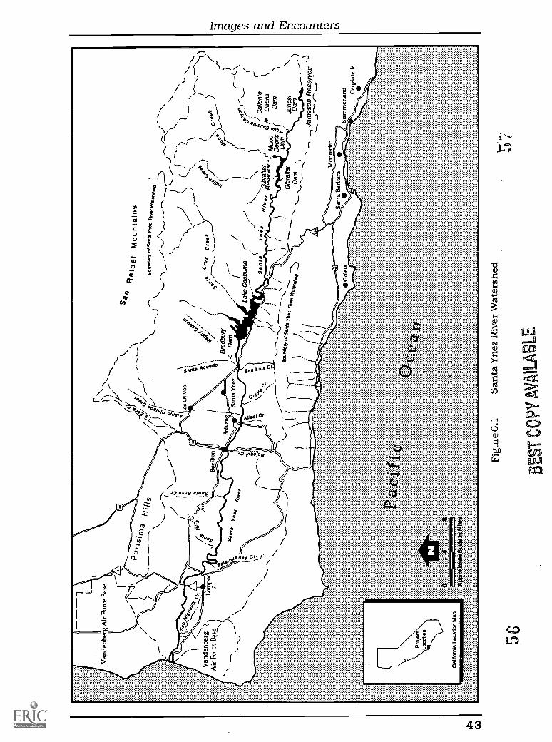
i-1
Van
denb
erg
Air
For
ce B
ase F
IN
7
6::1
4'...
,,Z"%
1
-N.4
4:,
Van
denb
erg
ZLo
mA
ir F
orce
Bas
e -...
\._m
/N\-
---
\
Pro
ject
Loca
tion
Cal
iforn
ia L
ocat
ion
Map
PU
risirn
a
101
Hill
s
\tt
-On
ft'
J
4
App
icki
mat
e W
ide
irk
Mite
s
Bue
llton
Paci
fic
San
Raf
ael
Mou
ntai
ns
Bou
ndar
y of
San
te T
hez
Aka
rW
aten
ihed
J
(
ur
Cr
Cre
ek)
eC
'°°1
,.,,\
cs)
s \
0(
$ko/
a.a.
+44
;7
/-I
-.1
r;(
Bra
dbur
y
es"
Vn"
Riv
o,
Sol
vang
..,.
i...
I"La
keC
achs
iimna
ta
----
(--
-/e
)monr
--.
_.--
,1
1
DIn
gs11
%go
b:\ )
Gib
ralta
rD
am t*
\I
(.)
-1--
-' 1int
a "'
BZ
Ft'V
ef W
at.;;
,..7
,.....
... ..
.....
.....
N...
. ,--
,-,
__)
----
- z-
- __
_-
Peen
1
Col
eta
15
\-r
Mon
teci
roS
anta
Bar
bara
Sum
mer
land C
arpi
nter
ia
56Fi
gure
6.1
Sant
a Y
nez
Riv
er W
ater
shed
BE
ST C
OPY
AV
AIL
AB
LE
Santa Barbara and California's Central Coast Region
Weather modification, in the form of cloud seeding to augment natural precipitationwithin winter storms, has been applied intermittently in Santa Barbara County during themajority of the winter seasons since 1950. Statistical studies showed that the naturalprecipitation above Jameson Lake or Reservoir (behind Juncal Dam) and GibraltarReservoir could be increased through cloud seeding efforts by an average of about 21percent during the October through April period. Winter storms are presently being seededin various parts of Santa Barbara County depending on hydrologic, watershed, andreservoir storage conditions.
Surface DiversionsSurface water diversions from the Santa Ynez River watershed are made primarily fromJuncal, Gibraltar,. and Bradbury dams. These facilities divert water for agricultural,municipal, and industrial uses in the Santa Ynez Valley and on the South Coast of SantaBarbara County.
Juncal Dam (Jameson Lake), completed in 1930, is owned and operatedby the MontecitoWater District. Diversions ofJameson Lake regulated flows, averaging 1,750 acre-feet peryear, are made to Montecito on the South Coast through the 2.14-mile (3.44-km) longDoulton Tunnel. Flows from Alder Creek can be diverted by flume into Jameson Lake. TheDoulton Tunnel intake location also allows for diversions from Fox Creek and for minordiversions of downstream tributary inflow. Tunnel infiltration is also delivered to Montecitoat a rate of about 400 to 500 acre-feet per year.
Gibraltar Dam was constructed by the City of Santa Barbara in 1920. GibraltarReservoir's constructed capacity of 14,500 acre-feet had been reduced because of siltationto about 7,600 acre-feet by 1947. The dam was subsequently raised 23 feet (7 m) in 1948to increase the capacity to 14,777 acre-feet. However, due to continuing siltation, GibraltarReservoir capacity has been reduced once again to about 8,600 acre-feet. Diversions fromGibraltar are made to the City of Santa Barbara through the 3.7-mile (5.95-km) longMission Tunnel. Annual diversions have ranged from more than 9,000 acre-feet in very wetyears to nearly zero in extreme drought years. Infiltration from Mission Tunnel is alsodelivered to the City.
Bradbury Dam (Lake Cachuma) was constructed by the U.S. Bureau of Reclamation in1950-1953 as part of the Cachuma Project. Diversions from Lake Cachuma are made tofive-member units, one in the Santa Ynez Valley and four on the South Coast, including theSanta Ynez River Water Conservation District; Improvement District #1, Goleta; the citiesof Santa Barbara, Montecito, and Carpinteria. Water is delivered to the Santa Ynez Valleyarea through a buried pipeline, and to the South Coast, through the 6.4-mile (10.3 km) longTecolote Tunnel. Tecolote Tunnel infiltration can also be delivered to the South Coastmember units at an average rate of about 2,000 acre-feet per year.
The minimum operating pool for Lake Cachuma is about 12,000 acre-feet. Diversionswhen the lake has 30,000 acre-feet or less in storage require pumps to deliver water to theSouth Coast member units, as was experienced for several months during the 1988-91drought. In recent years, annual diversions from Lake Cachuma have been as high as31,021 acre-feet. These diversions exceeded the recently reevaluated Lake Cachumaoperational target yield of about 25,908 acre-feet per year. As a result of these relativelyhigh diversions in the early years of the drought, only 17,000 acre-feet could be deliveredin 1990, about a 40 percent reduction from normal.
Historical Flood FlowsSeveral major flood events occurred along the Santa Ynez River over the past 100 yearsin 1907, 1914, 1938, 1969, and 1978. Reported peak discharges for these storms rangedfrom 45,000 to 120,000 cubic feet per second (cfs), and the floods caused much damage tothe Lompoc Valley. The most devastating flood occurred in January and February 1969.Although the 1969 flood was reportedly lower in magnitude than the 1907 flood, it causedmore damage because the county was relatively undeveloped in 1907.
44r- r,J
Images and Encounters
The river channel capacities vary greatly along the river below the dam. With theexception of the 1969 floods, river channel capacities have been adequate to passhistoric flood flows without damage to urban areas such as Solvang, Buellton, andLompoc. However, past flood events have caused flooding and erosion to undevelopedand agricultural lands, and have damaged or destroyed numerous bridges at variouslocations along the river.
Riparian growth in the Santa Ynez River channel west of Lompoc has been enhancedby the effluent from the Lompoc Regional Wastewater Treatment Plant, and flooding ofagricultural lands to the west is of particular concern. The dense vegetation in the riverchannel creates a flood hazard by reducing the conveyance capacity. In addition, itreduces water velocities, which in turn, increase sediment deposits that furtherdecrease the capacity. Finally, trees in the riverbed can become uprooted during floodevents and block the channel under bridges thereby causing additional floodingupstream and serious damage to the bridges. Some vegetation cutting has been done,and a long term channel maintenance project is currently being developed by the Countyof Santa Barbara Flood Control District to improve channel capacity, however, to datethe required permits have not been acquired. The river channel capacity is currentlybelow 20,000 cfs. In 1993 and 1995, several events of approximately 15,000 to 17,000 cfsbarely passed through the constricted reach, and flooding occurred in 1993 on theadjacent low-lying agricultural fields.
Cachuma Project Facilities: Bradbury Dam and Lake CachumaBradbury Dam is located on the Santa Ynez River approximately 25 miles (40.23 Ian)northwest of Santa Barbara. It is an earth-filled structure with a structural height of 190feet (58 m). The spillway crest is at elevation 720 feet (219 m) and the top of the spillwaygates is at elevation 750 feet (229 m). An outlet at the base of the dam has a maximumcapacity of 300 cfs; however, it is rarely used above 100 cfs. The reservoir, LakeCachuma, has a surface area of 3,043 acres (1,232 ha). The original reservoir capacitywas 205,000 acre-feet, but the capacityhas been reduced by siltation to 190,406 acre-feet. The Bureau of Reclamation established the dead pool at elevation 600 feet (183 m)and has a capacity of 12,000 acre-feet.
Conveyance FacilitiesWater from Lake Cachuma is conveyed to the South Coast member units through theTecolote Tunnel intake tower at the east end of the reservoir. The seven-foot diameterTecolote Tunnel extends 6.4 miles (10.3 km) through the Santa Ynez Mountains fromLake Cachuma to the headwaters of the South Coast Conduit. The South Coast Conduitis a high pressure concrete pipeline that extends from the Tecolote Tunnel outlet to theCarpinteria area, a distance of more than 24 miles (39 km), and includes four regulatingreservoirs. The Sheffield Tunnel is located along the conduit. This mile-long (1.6 km)concrete tunnel was bored through a high ridge within the city limits of Santa Barbara.The South Coast Condiiit extends through the tunnel. Water is delivered to the SantaYnez Valley through Bradbury Dam's outlet works into theSolvang-Santa Ynez Conduit.
Groundwater Resources: South Coast BasinsFour major South Coast groundwater basins are used by the member units. Thesebasins lie between the Santa Ynez Mountains to the north and the Pacific Ocean to thesouth. They are the Carpinteria Basin, the Montecito Basin, the Santa Barbara Basin,and the Goleta Basin.
The South Coast groundwater basins are bordered by the mountains and relatively non-water yielding rocks on several sides and the ocean on thesouth side. The basins consistof layers of coarse-grained, water transmissive sedimentary units, interbedded withfine-grained less transmissive units. Wells are typically drilled to great depths(hundreds to a thousand feet below groundwater surface) and are completed to producefrom multiple vertical intervals so as to draw water from as many water transmissiveunits as possible. Historically, and during extended wet periods, groundwater levels insome wells rise above land surface because some of the transmissive units are confined
S 45
Santa Barbara and California's Central Coast Region
aquifers. Groundwater in overlying transmissive units is recharged at higher elevations inthe basins (commonly from short coastal streams exiting canyons), which in effect fillsconfined portions of the aquifers, causing the aquifers to be pressurized in lower elevationsof the basins. When the pressure becomes large enough, flowing wells will result.
The South Coast basins are recharged by seepage from streams, percolation ofprecipitation, subsurface inflow from materials underlying the Santa Ynez Mountains, andreturn flow of imported water such as surface water from Lake Cachuma. Much of therecharge occurs along the northern boundaries of the basins, where the water transmissiveunits that extend deep into the basins are exposed at or near the surface. Therefore, mostrecharge occurs in periods of extended rainfall and less recharge occurs in dry periods orwhen rainfall and runoff occur over short periods. Discharge from the basins is to the ocean,to pumping, and to a limited extent, to streams at lower elevationsin the basins. In general,the pattern of groundwater flow follows the surface topography ofthe basin, from areas ofhigh elevation towards the ocean. Pumping has become the most significant dischargecomponent since the turn of the century.
The Carpinteria Groundwater Basin is an elongate northwest-southeasttrending basinthat occupies approximately 7,620 acres (3,085 ha) and is separated into two storage unitsby the Rincon Creek Thrust Fault. Pumping of the basin occurs both by the CarpinteriaValley Water District and by a large number of agricultural users operating private wells.
The Montecito Groundwater Basin is a smaller basin of 4,300 acres (1,741 ha) locatedbetween the Santa Ynez mountains to the north, the offshore Rincon Thrust Fault to thesouth, the Carpinteria Basin to the east, and the Santa Barbara Basin to the west. Althoughthe Montecito and Santa Barbara Basins are hydrologically connected, the boundarybetween them follows a politically-designated line.
A topographic divide west of Arroyo Burro Creek is generally accepted as the boundarybetween the Goleta and Santa Barbara Basins. The southern boundary is an offshore fault,which reportedly seals off the lower aquifers from the ocean. The Mesa and Mission RidgeFaults divide the Santa Barbara Basin into three storage units which together currentlyhave a usable storage of approximately 10,000 acre-feet. The basin, pumped bythe City formunicipal and industrial use, occupies an area of about 7,400 acres (2,996 ha) in andaround the City of Santa Barbara.
The Goleta Groundwater Basin is a narrow east-west trending basin, between the SantaYnez Mountains to the north and the More Ranch Fault to the south. The basinis more thaneight miles (12.9 km) long and up to four miles (6.5 km) wide, occupying approximately 9,200acres (3,725 ha). The Modoc and Goleta Faults run through the interior of the basin,however, the Goleta Fault is not thought to be an effective groundwater barrier, so thecentral and north subbasins are now considered to be one unit. Groundwater levelsfluctuate in response to changes in pumping, injection, and precipitation, and declined bymore than 50 feet ((15.2 m) between 1971 through 1989. Groundwater levels appear to berecovering because of injection and significant reductions in pumping since 1989 by theGoleta Water District.
Groundwater Resources. Downstream BasinsFive groundwater basins lie along the Santa Ynez River downstream of BradburyDam: theSanta Ynez River Riparian Basin, the Santa Ynez Uplands Basin, the Buellton UplandsBasin, the Santa Rita Uplands Basin, and the Lompoc Basin.
Groundwater Resources: Santa Ynez River Riparian BasinThe Santa Ynez River Riparian Basin comprises shallow alluvial material adjacent to, andhydrologically connected with, the Santa Ynez River. The basin is approximately 36 miles(58 km) long, and has been subdivided into the Santa Ynez subarea; the Buellton subarea;and the Santa Rita subarea. The total storage capacity of the alluvial deposits is about105,000 acre-feet.
46 by
Images and Encounters
Groundwater storage and groundwater levels fluctuate in response to streamflow, releasesfrom Bradbury Dam, groundwater pumping, and to a lesser extent, other recharge anddischarge conditions. Groundwater storage and water table elevations generally increaseduring winter and spring, and other wet periods, when flow in the Santa Ynez River loseswater to the underlying alluvial aquifer. Under average water supply conditions, netdemand from the riparian basin does not exceed recharge, however, monitoring wellsshowed that storage did decline during the recent drought indicating that demand is greaterthan recharge under thy conditions. The riparian basin usually becomes full shortly afterthe onset of wet conditions and then it no longer accepts additional water. Surface waterwill pass through the basin with very little percolation under high streamflow conditions orwhen the basin is full.
Groundwater storage and groundwater levels decrease in the riparian basin duringsummer, fall, and dry periods through pumping, groundwater discharge back into the riveras base flow, and by underflow through the alluvium downstream toward the Lompoc Basin.The longer the dry period, the greater the decline in groundwater storage and elevation. Theupper reaches of the riparian basin will drain first, analogous to a long pipe at one end.Therefore, if a dry period is long enough, the upper reaches of the riparian basin may draincompletely even though the lower reaches may remain full.
Groundwater Resources: Santa Ynez Uplands and Buellton BasinsThe Santa Ynez Uplands and Buellton Basins are large groundwater basins that do notreceive recharge from the Santa Ynez River. In these basins, typical hydrologic processes,such as recharge by precipitation and streams, and discharge by pumping and subsurfaceoutflow, largely control groundwater storage and groundwater levels.
The Santa Ynez Uplands groundwater basin is the largest in the county occupying about88,000 acres (35,628 ha). The main water-bearing units are the continental, Plio-Pleistocene Paso Robles Formation and the marine, Pliocene Careaga Sand. The totalgroundwater usable storage today is estimated to be 900,000 acre-feet. The perennial yieldof the basin is currently about 11,500 acre-feet per year, which is somewhat greater thanthe annual recharge.
The Bue llton Uplands groundwater basin occupies about 16,400 acres (6,640 ha) northof the Santa Ynez River near the City of Buellton. The basin is bounded by bedrock outcropsto the north and south, a narrow connection to the Santa Ynez Uplands Basin to the east,and a groundwater divide on the west with the Lompoc Basin.
Groundwater Resources: Lompoc BasinThe Lompoc Groundwater Basin occupies an area of approximately 48,600 acres (19,676).This basin comprises three subareas including the Lompoc Plain, the Lompoc Terrace, andthe Lompoc Basin. These subareas are hydrologically connected so they are often treatedtogether along with the Santa Rita Uplands Basin, for the purposes of determining storageand perennial yield. The Lompoc Plain is the only subarea of the Lompoc Basin that receivesrecharge directly from the Santa Ynez River.
It is estimated that the total available groundwater storage in the Lompoc Basin is170,000 acre-feet, 135,000 acre-feet of which is stored in the Lompoc Plain. Recharge to theLompoc Plain comes from percolation of precipitation, seepage from the Santa Ynez River,agricultural return flows, sewage effluent, and underflow from deeper aquifers of theLompoc Terrace and Basin, which extend beneath the plain. In addition, recharge thatwould have occurred but does not because of the operation of Bradbury Dam is calculatedand credited to a Lompoc water account known as the Below Narrows Account. The accountwater is stored in Lake Cachuma and is released in such a way that it recharges the LompocPlain.
61
BEST COPY AVA!LARLF
47
Santa Barbara and California's Central Coast Region
As this chapter has illustrated, water in Santa Barbara County has always been, and willcontinue to be, a precious resource. As urban populations expand around dense nodes ofsettlement at, for example, Santa Barbara, Montecito, Carpinteria, Goleta, and Lompoc, theavailability of a clean water supply will become an increasingly important consideration inthe new century.
6
48
7
Agricultural Patterns in Ventura County'sHeartlandChris MainzerDriving through Ventura County's heartland along U.S. 101, the major coastal routebetween Los Angeles and San Francisco, the traveler is suddenly struck by the abundanceand variety of irrigated fields of tree crops, fruits, vegetables, and flowers that cover theOxnard Plain and nearby river valleys (Figure 7.1). The bountiful agricultural harvests fromthis broad stretch of coastal plain, a mere 60 miles (97 km) from the Los Angeles CivicCenter, are possible under southern California's sunny skies and the moderatinginfluences of the Pacific Ocean. Ventura County's top ten cash crops of lemons, celery,strawberries, nursery stock, avocados, oranges, lettuce, cut flowers, broccoli, and cabbageall flourish under ideal climatic conditions (Tables 7.1 and 7.2).
The Southland's climate is often described as Mediterranean, or of dry subtropicalcharacter. The average precipitation for the Oxnard region is only 15 inches (38 mm)annually. The wet season, influenced by the Westerlies pattern, usually extends fromNovember through March producing very mild winters, in sharp contrast to long periods ofsummer drought dominated by a subtropical high pressure system. The coastal site of thisrich agricultural belt in Ventura County further enhances a low yearly temperature rangeof 12°F (8°C) with a 62°F (17°C) average annual temperature. The ocean provides a cool,marine layer and a summer sea breeze cycle that maintains a high relative humidity, and,that in winter, reduces the risk of frost damage to the high value crops grown in the area.
An example of how crucial is the marine influence can be seen in a visit to the SeasideBanana Garden at La Conchita, ten miles (16 Ian) northwest along the coast (near RinconPoint) from the city of Ventura. This 12-acre (4.9 ha) plantation raises more than 50 varietiesof bananas, normally associated with tropical climates such as those found in Hawaii, LatinAmerica, Asia, or Africa, and is a one-of-a-kind farm operation in the continental UnitedStates. Buffered by the Pacific Ocean on one side and sheltered from inland temperatureextremes on the other side by a 300-foot (92 rn) high sea cliff, it has become a unique culturalfeature on the Ventura shoreline.
Arable LandsArable lands occupy only one-third of the county's total land area, the rest of the region issomewhat mountainous and primarily of high relief. The calcium-rich, sandy-to-silt loamsoils of the coastal alluvial lowland and adjacent stream valleys are remarkably fertile andafford excellent drainage for irrigated crop production. The natural stream- laid deposits ofclay, silt and sand, especially from the Santa Clara River, have contributed to the deep andrich mineral quality of the Class I soils of the Oxnard Plain.
WaterBecause the region receives sparse rainfall in summer, water is a precious commodity. Inorder to make commercial agriculture succeed, imported water from the State Water Projectmust be allocated for farming this semi-arid alluvial plain. This much-needed water beginsits long journey in northern California's huge Oroville Reservoir that is part of the state'sFeather River project, and travels almost 450 miles (724 km) to its final destination ineastern Ventura County's Lake Piru facility. Local well water has also been mined since the1890s from some of the deep-seated aquifers below the Oxnard Plain and supplements thefresh water supply for Ventura County. This last action has triggered the gradual process
63
49
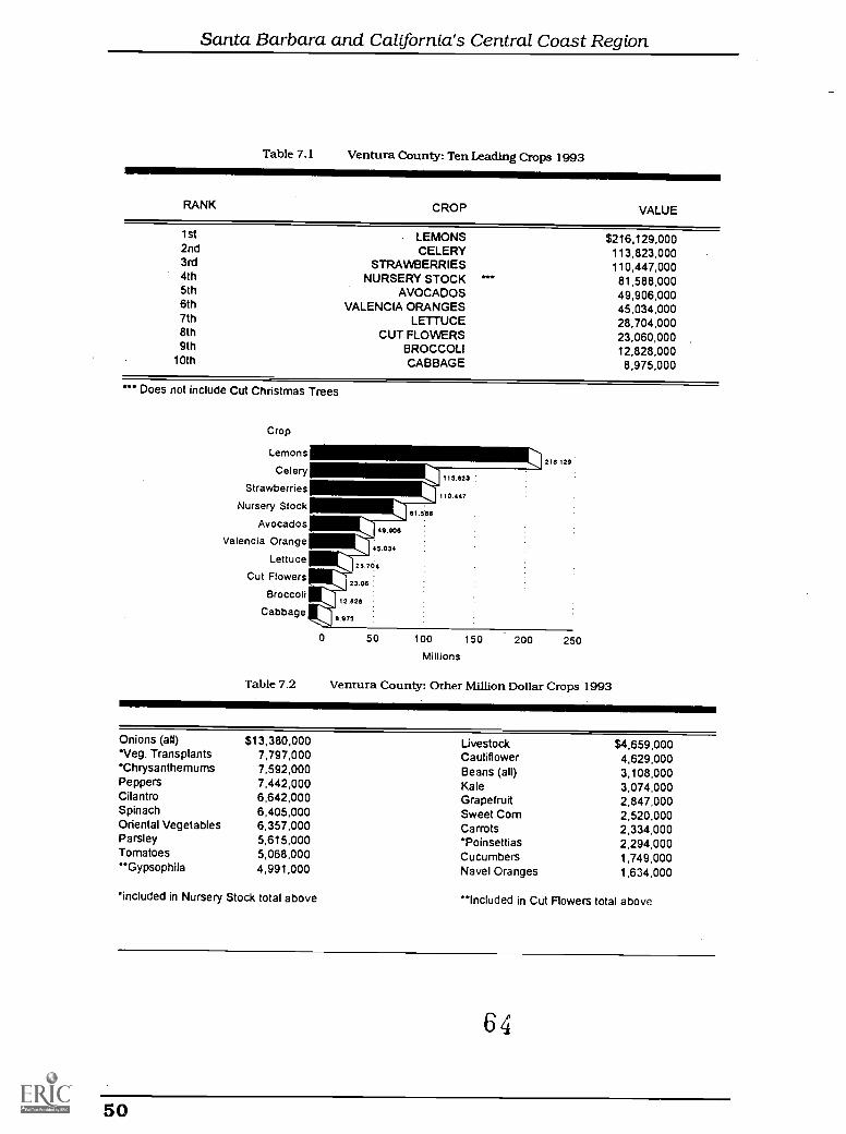
Santa Barbara and California's Central Coast Region
Table 7.1 Ventura County: Ten Leading Crops 1993
RANK CROP VALUE
1st LEMONS $216,129,0002nd CELERY 113,823,0003rd STRAWBERRIES 110,447,0004th NURSERY STOCK ... 81,588,0005th AVOCADOS 49,906,0006th VALENCIA ORANGES 45,034,0007th LETTUCE 28,704,0008th CUT FLOWERS 23,060,0009th BROCCOLI 12,828,000
10th CABBAGE 8,975,000
***Does not include Cut Christmas Trees
Crop
Lemons
Celery
Strawberries
Nursery Stock81 51511
Avocados
Valencia Orange
Lettuce
Cut Flowers
Broccoli
Cabbage
111.11111C417808
45 034
25 704
23.08
12.820
0.973
218.129
113 823
110 447
0 50 100 150 200 250
Table 7.2
Millions
Ventura County: Other Million Dollar Crops 1993
Onions (all) $13,380,000 Livestock $4,659,000'Veg. Transplants 7,797,000 Cauliflower 4,629,000'Chrysanthemums 7,592,000 Beans (all) 3,108,000Peppers 7,442,000 Kale 3,074,000Cilantro 6,642,000 Grapefruit 2,847,000Spinach 6,405,000 Sweet Corn 2,520,000Oriental Vegetables 6,357,000 Carrots 2,334,000Parsley 5,615,000 *Poinsettias 2,294,000Tomatoes 5,068,000 Cucumbers 1,749,000**Gypsophila 4,991,000 Navel Oranges 1,634,000
*included in Nursery Stock total above "Included in Cut Flowers total above
64
50
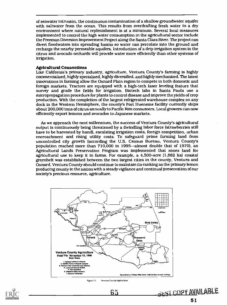
of seawater intrusion, the continuous contamination of a shallow groundwater aquiferwith saltwater from the ocean. This results from overdrafting fresh water in a dryenvironment where natural replenishment is at a minimum. Several local measuresimplemented to control the high water consumption in the agricultural sector includethe Freeman Diversion Improvement Project along the Santa Clara River. The project candivert floodwaters into spreading basins so water can percolate into the ground andrecharge the nearby permeable aquifers. Introduction of a drip irrigation system in thecitrus and avocado orchards will provide water more efficiently than other systems ofirrigation.
Agricultural ConnectionsLike California's primary industry, agriculture, Ventura County's farming is highlycommercialized, highly specialized, highly diversified, and highly mechanized. The latestinnovations in farming allow the Oxnard Plain region to compete in both domestic andforeign markets. Tractors are equipped with a high-tech laser leveling feature thatsurvey and grade the fields for irrigation. Biotech labs in Santa Paula use amicropropagation procedure for plants to control disease and improve the yields of cropproduction. With the completion of the largest refrigerated warehouse complex on anydock in the Western Hemisphere, the county's Port Hueneme facility currently shipsabout 200,000 tons of citrus annually to Pacific Rim consumers. Local growers can nowefficiently export lemons and avocados to Japanese markets.
As we approach the next millennium, the success of Ventura County's agriculturaloutput is continuously being threatened by a dwindling labor force (strawberries stillhave to be harvested by hand), escalating irrigation costs, foreign competition, urbanencroachment and rising utility costs. To safeguard prime farming land fromuncontrolled city growth (according the U.S. Census Bureau, Ventura County'spopulation reached more than 710,000 in 1995almost double that of 1970), anAgricultural Lands Preservation Program was implemented that zones land foragricultural use to keep it in farms. For example, a 4,500-acre (1,882 ha) coastalgreenbelt was established between the two largest cities in the county, Ventura andOxnard. Ventura County should continue to maintain its ranking as the primary lemonproducing county in the nation with a steady vigilance and continual preservation of oursociety's precious resource, agriculture.
mem
Simi Valley
41,.../ 4E1venturalM
re,
Pal Mee. » la
O
Ventura County AgricultureField Trip November 13, 1996
Major Stops
1. Saticoy Lemon In Venture2. Clebich Fenn In Wheeler Canyon
3. Freeman Dam Diversion near SaUcoy4. Lunch at Venture Harbor
5. Port HuenemeS. Pleasant Valley Nursery
7. Bane= PlantatIon
housandOaks
Map prcduesd by Rohm= Warn Boren Cassia Sisto unevenly, Montridge
Figure 7.1 Ventura County Agriculture
61S COPY AVAILABLE51
Wines of Santa Barbara County:A Geographic Perspective
Vatche P. Tchakerian and Robert S. BednarzThe viticultural area in Santa Barbara County (known as the South Central Coast), is atriangular region roughly enclosed by the cities of Santa Maria and Lompoc on the west, toSanta Ynez and San Marcos Pass on the east. In this relatively small geographic region, morethan 9,700 acres (3,927 ha) of vineyards yield an average of four tons/acre (9.88/ha). Theunique geomorphologic setting, climate, soils and the ability of the winemakers to takeadvantage of these characteristics, have made the region one of the premier producers ofexcellent wines and has allowed it to take its rightful place alongside its more famousneighbors to the north.
Historic BackgroundHistorically, the region has been known primarily for cattle grazing and farming. The earliestwinemaking attempts began with the Spanish missions in the late eighteenth century. Notuntil the mid-1960s, however, were modern vineyards planted. The landmarkestablishments of Firestone Vineyard, Zaca Mesa Winery and Rancho Sisquoc Winery dateback only to the early 1970s. These and other early wineries took advantage of the low costof land, excellent climate, and a unique geomorphic environment (Figure 4.1). One of thereasons earlier attempts in viticulture met with limited success, is that wine growersperhaps placed too much emphasis on such Bordeaux varieties as Cabernet Sauvignonrather than varieties better suited to the climatic and soil conditions of the area.
Physical GeographyThe physical geography of today's South Central Coast is primarily the result of the geologicmovements (still continuing) associated with the formation of the San Andreas Fault and theresulting Transverse Ranges. The latter, one of two major east-west trending mountainranges in the United States, begins as the San Bernardino Mountains (to the southeast) andcontinues westward and ends as the Santa Ynez Mountains.
The Santa Barbara viticulture region is bounded on the north by the Sierra Madre andSan Rafael Mountains, on the south and east by the Santa Ynez Mountains, and on the westby the Pacific Ocean. Between these ranges, east-west-trending valleys open to the PacificOcean (Figure 4.1). During the late spring and most of the summer, coastal fog, developedbecause of the presence of the cool, California Current off the coast, surges inland, along withlight winds and higher humidities, thus keeping temperatures moderate (see Chapter 4).
The cool, coastal winds and fog have their greatest influence on those vineyards closestto the coast. The continentality effect is most pronounced on vineyards farthest from thecoast, since the fog dissipates with distances inland, both spatially and in intensity.Therefore the vineyards located closest to the foothills of the main ranges in the easternmostsection of the county tend to have higher daytime temperatures, higher potentialevapotranspiration rates, and higher soil temperatures (requiring more moisture intakethan those at lower elevations). Because of these climatic variations, the vineyards closestto the coast are similar to the Burgundy region of east-central France (hence the first-ratePinot Noirs from Sanford). On the other hand, the vineyards in the warmer interiors areclimatically similar to Bordeaux (southwestern France) and the southern RhOne(southeastern France).
66
52
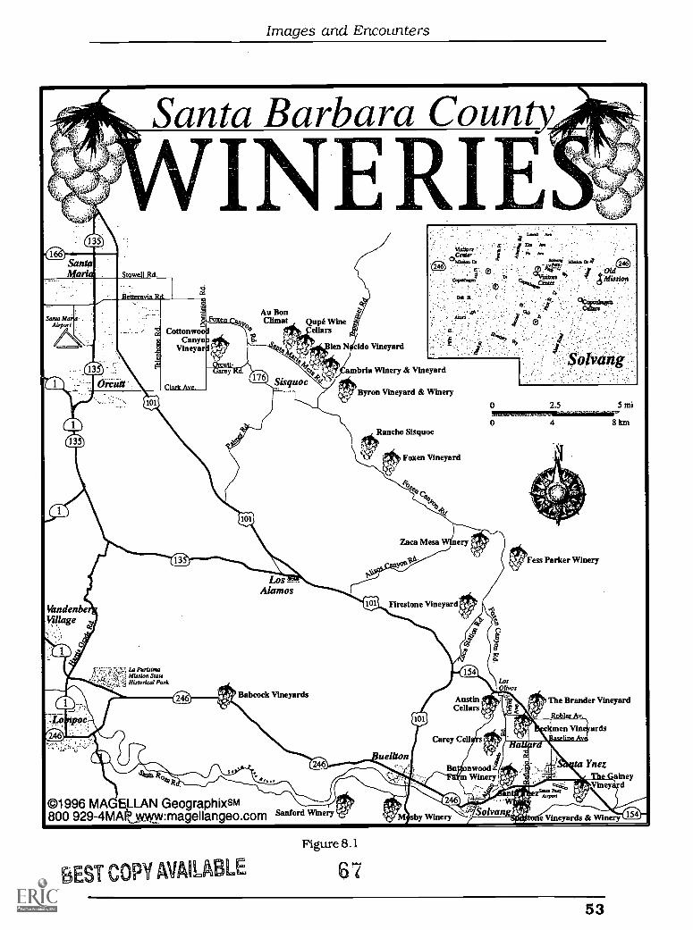
Images and Encounters
Santa Barbara Coun
Stowell Rd
OSIsorsaCatur
Oak St
Santa hfAirport 8
CottonwCanyo
Vineyar
Au BonClimattyJ
f6
Qupe Wineellars
cido Vineyard
Sisquocambria Winery & Vineyard
Byron Vineyard & Winery
Rancho Sisquoc
0
Foxen Vineyard
kt
LosAlamos
limdenbectqage
Firestone Vineyard*
Babcock Vineyards
LosOlivos
Fess Parker Winery
AustinCellars
5 mi
8 km
The Brander Vineyard
Roblar Av
en Vin ardsCarey Cell
uellton
0,nwoodWinery
©1996 MAGELLAN Geographixsm800 929-4MAFtwy:magellangeo.com
BEST COPY AVAILABLE
ta Ynezainey
Sanford Winery
Figure 8.1
67
sby Winery Solvane Vineyards & Winery
53
Santa Barbara and California's Central Coast Region
Microclimate is one of the most important geographic factors controlling the productionof wines. The vineyard owners and winemakers of Santa Barbara County analyzed themicroclimates of the region in great detail, leading to the proper selection of vineyard sitesand grape varieties. The proper understanding of factors such as the spatial and temporalvariability of the coastal fog during the critical months of May through August, vineyardaspect (north-south facing slopes), microtopography, wind speed (persistence, direction,turbulence, mixing) and evapotranspiration, and a detailed knowledge of soils andgeomorphology played a key role in the success of this viticulture region.
The vineyards follow closely the microtopography of the South Central Coast (Figure 1.2).Typical vineyard elevations are between 200 and 1,500 feet (61 and 457 m). Because of thepresence of various soil subtypes in this geomorphologically varied region, wine makershave been able to match the different soil types to those grape varieties that do best undergiven soil conditions. River valleys, terraces, floodplains and inteffluves, along with theirsoils, have all been studied and analyzed in great detail and vines planted accordingly.
Wines and WineriesThe area is home to more than 30 wineries, more than 75 percent of them established after1982 (Figure 8.1). Approximately 400,000 cases of wine are produced annually. About 35percent of the grapes grown in this geographical region are crushed by local wineries.Although all major grape varieties are produced successfully, the reputation of the regionrests firmly on the excellent qualities of Pinot Noir, Chardonnay, andmore recently, Syrahand other southern Rhone-type varieties. The two distinct and approved viticulture regionsin Santa Barbara County include the Santa Maria Valley in the northern part and theSanta Ynez Valley in the southern part. Among the excellent wineriesare such establishednames as Firestone, Rancho Sisquoc, Sanford, Santa Ynez, and Zaca Mesa. A second waveof vintners such as Au Bon Climat, Byron, Fess Parker, Foxen. and Qupe, along with manyothers, have continued to push the region's wines to an outstanding level, particularly withtheir innovative techniques for matching the right grape varieties to the physical geographyof the region as well as in pooling resources and wine-making infrastructures (such assharing the Central Coast Wine Warehouse in Santa Maria). One of the most famous andlargest vineyards is the 600-acre (243-ha) Bien Nacido Vineyard in the Santa Maria Valley,which sells its fruit to numerous wineries in the region and outside. Some of the most soughtafter chardonnays from Au Bon Climat and syrahs from Qupe come from this vineyard.
Keeping in mind the vicissitudes and vagaries of the climate (as witnessed by heavy rainsand unusually cold weather in the spring of 1995), the high quality of wines, the dedicationof grape growers and winemakers, and the planting of new acreage in vines, thisrenaissance in Santa Barbara County wines will most likely continue and increase in thenear future.
68
54
Images and Encounters
9
The View from Paradise:Problems and Prospects of the CaliforniaCentral CoastWilliam C. HalperinLisa Knox BurnsVentura, Santa Barbara, and San Luis Obispo counties make up the '1'i-1-County area of theCalifornia Central Coast. In the southeast portion of Ventura County, the Conejo Grade (onHighway 101 where it intersects with Route 23) acts as a physical barrier to the tentaclescf Los Angelization. Similarly, Santa Barbara County on its southeastern border isfortunate to have a 30-mile (48 km) greenbelt between it and the City of San Buenaventura(the official name for Ventura). In this narrow stretch of Highway 101, fragile palisades withsteep slopes make urban development prohibitive. Here one only finds the small, scatteredresidential enclaves of Solimar-Faria Beach, Sea Cliff, La Conchita, and Mussel Shoals. TheSanta Barbara County line begins at Rincon Point, a famous surf break .
Summary of Geographical PhenomenaSanta Barbara County comprises nearly 2,750 square miles (7,123 sq kin) of land andinland water area (about 1.45 times the size of the state of Delaware). Approximatelyrectangular in shape, Santa Barbara County is bordered on the north by San Luis ObispoCounty, on the east by Ventura County, and on the south and west by 107 miles (172 km)of Pacific coastline. Facing south rather than west, the south coast of Santa Barbara isgeographically unique among California coastal areas. The Santa Ynez Mountains, part ofthe Transverse Ranges behind Santa Barbara, extend predominately in an east-westdirection, the only range system on the West Coast where this occurs. Along the south coasta relatively narrow strip of coastal valleys and foothills, no greater than six miles inwidth,stretches from Carpinteria on the east to Gaviota at the west end (see Figures 1.2 and 4.1).The California Channel Islands of Santa Rosa, San Miguel, Santa Cruz, Anacapa, SanClemente, and Catalina buffer the coastline. Both on land and in the sea, Santa BarbaraCounty is blessed with abundant habitats as it is the northernmost extent of flora and faunacommon to southern California, and the southernmost extent of flora and fauna commonto northern California. The largest variety of birds in the nation can be found in SantaBarbara during the winter months, according to annual estimates made by the AudubonSociety.
Economics of the AreaWithin Santa Barbara County are numerous fertile agricultural areas, including the SantaMaria, Cuyama, Lompoc, and Santa Ynez Valleys, and the southeast coastal plain. Theseareas, which include most of the developed land, also accommodate the majority of thepopulation. Los Padres National Forest, in the eastern part of the county, coversapproximately 44 percent of the total county area (see Figure 1.2). As one drives northleaving the City of Santa Barbara, the cities and towns become widely spaced nodes ofurban development, surrounded by open space and agricultural land. Locals have reportedthat pundits have described Santa Barbara County as a little like Disneyland. Frontierlandcan be found in the historic towns of SantaYnez, Ballard, and Los Olivos. Solvang looks likea Danish town. Vandenberg Air Force Base (VAFB), where Titan rockets are launched fromSLC-6 (-Slick-six"), is Tomorrowland. The City of Santa Barbara is a Fantasyland dressedin red-tile roofs and bougainvillea vines. The rest of the joke states that public restroomscan be found in Santa Maria.
BEST COPY AVAILABLE
55
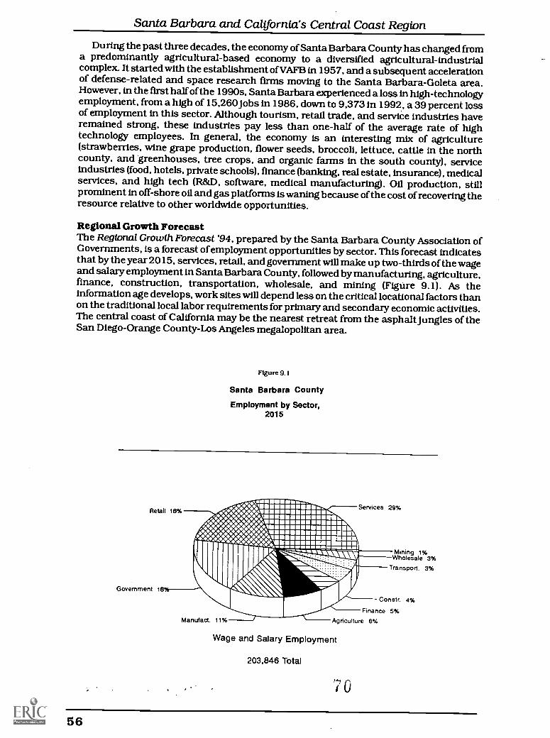
Santa Barbara and California's Central Coast Region
During the past three decades, the economy of Santa BarbaraCounty has changed froma predominantly agricultural-based economy to a diversified agricultural-industrialcomplex. It started with the establishment of VAFB in 1957, and a subsequent accelerationof defense-related and space research firms moving to the Santa Barbara-Goleta area.However, in the first half of the 1990s, Santa Barbara experienced a loss in high-technologyemployment, from a high of 15,260 jobs in 1986, down to 9,373 in 1992, a 39 percent lossof employment in this sector. Although tourism, retail trade, and service industries haveremained strong, these industries pay less than one-half of the average rate of hightechnology employees. In general, the economy is an interesting mix of agriculture(strawberries, wine grape production, flower seeds, broccoli, lettuce, cattle in the northcounty, and greenhouses, tree crops, and organic farms in the south county), serviceindustries (food, hotels, private schools), finance (banking, realestate, insurance), medicalservices, and high tech (R&D, software, medical manufacturing). Oil production, stillprominent in off -shore oil and gas platforms is waning because of the cost of recovering theresource relative to other worldwide opportunities.
Regional Growth ForecastThe Regional Growth Forecast '94, prepared by the Santa Barbara County Association ofGovernments, is a forecast of employment opportunities by sector. This forecast indicatesthat by the year 2015, services, retail, and government will make up two-thirds of the wageand salary employment in Santa Barbara County, followed by manufacturing, agriculture,finance, construction, transportation, wholesale, and mining (Figure 9.1). As theinformation age develops, work sites will depend less on the critical locational factors thanon the traditional local labor requirements for primary and secondaryeconomic activities.The central coast of California may be the nearest retreat from the asphalt jungles of theSan Diego-Orange County-Los Angeles megalopolitan area.
Figure 9.1
Santa Barbara County
Employment by Sector,2015
Government 18
Mining 1%Wholesale 3%
Transport. 3%
Constr. 4%
Finance 5%Agriculture 8%
Wage and Salary Employment
203,846 Total
70
56
Images and Encounters
San Luis Obispo and Santa Barbara counties have restrained rampant urban growthprimarily because the urban service infrastructure, particularly for water, was limited. SanLuis Obispo and Santa Barbara counties rely almost exclusively on recapturing rain waterto supply urban needs. Vast groundwater basins under Paso Robles in San Luis ObispoCounty and Santa Maria in Santa Barbara County have been mined in recent years tosupply water. Coastal cities such as Goleta, Santa Barbara, and Montecito in SantaBarbara County, and Cambria, Cayucos, Morro Bay, and Los Osos in San Luis ObispoCounty have faced periods of severe restrictions for municipal water use. Some communitieshave had long-standing moratoria on new water hook-ups. The scarce water situation forsome communities, however, mainly in Santa Barbara County, is about to change with theaddition of the State Water Project (SWP) supplies in 1997. The SWP is nearly complete fromPolonio Pass on Highway 46 in northeastern San Luis Obispo County to Lake Cachumaalong Highway 154 in Santa Ynez Valley where the Central Coast Water Authority pipelineterminates. According to estimates, 1,500 residential units in Goleta alone are pendingdevelopment, as they await the arrival of state water.
Preserving the Quality of LifeThe debate in the coming years will center on whether persons in elected and appointedoffices who control comprehensive plans and zoning permits, can retain the small towncharm of Santa Barbara and San Luis Obispo counties, and resist the homogeneity thatregional shopping centers, fast-food restaurants, and residential planned developmentsbring. For Santa Barbara and San Luis Obispo, growth has been kept in check and in linewith environmental resources. As the lack of potable water recedes as a rationale forcontrolling growth, other issues such as traffic, air quality, and agricultural landpreservation become the focus of citizens concerned with preserving our quality of life.Quality of life is a priceless commodity that most people who live in Santa Barbara and SanLuis Obispo value highly enough to forgive the little negatives of living in paradise: highhousing prices, lack of megastore outlet centers, fewer chain stores, more one-way streets,and higher gasoline prices.
7i
57
10-A
Lesson Plan A
Weather or Not:Making and Using a Climograph
Terry Williams and Jerry R. Williams
California is generally described as having a Mediterranean climate; in reality, the statehas a variety of different climates. Description of climate are based on the long-term (30years) statistical averages of the atmospheric conditions of temperature and precipitation(weather) in a particular location. Weather varies from day to day whereas climates tendto be stable and change only slowly over time. The climate of a particular location isinfluenced by such factors as: latitude, elevation, mountain barriers, ocean currents, airmasses, pressure cells, storms, and continentality (interior vs. coastal locations). Climateis an abstract concepta mental construct, but one that we frequently use to describe thecharacter of places. Climographs are charts used to record climate data.
Level: Middle and Secondary Schools
Objectives *(See sources on geographic skills and perspectives and standards at the endof this lesson.)
To practice graphing climatic data for a specific location on a climograph.To compare climates in various locations and hypothesize on the local influences of
latitude, elevation, and mountain barriers.To discuss how climate affects the daily life of local inhabitants.
Procedure1. Introduce the concept of weather and climate by comparing recent events in California:
the six-year drought, the unusually wet winter of 1992-1993 with floods and heavywinter snow pack.
2. Use a transparency to demonstrate a climograph and how to plot climate data on aclimograph.
3. Graph climate data from one of the locations on the data sheet.4. Prepare photocopies of the climograph and climate data and distribute to students
or perhaps to pairs or small groups of students.5. Locate and label (or circle) each of the cities from the data sheet on a wall map of
California or on a California base map. See Lesson Plan B for county base map ofCalifornia.
6. Post the completed climograph for each city above its location on the map.7. Compare the climographs for various Northern California locations and discuss the
major factors that influence the amount and distribution of precipitation andtemperature ranges.
8. Repeat procedure #7 using Central California, Southern California, and CoastalCalifornia.
9. Discuss how climate affects the daily life, throughout the year, of a student living ina coastal location, central location, and eastern location.
58
Images and Encounters
ExtensionsPrepare a climograph for other locations in the United States and compare them to those fromCalifornia. Possible locations might include New York City, Chicago, Miami, Denver, Tucson,Cheyenne, St. Louis, and New Orleans. Do the same with cities from around the world, perhapsat similar latitudes (see U.S. and World base maps at end oflesson).Use the weather section from a local newspaper to compile a record of local temperatures andprecipitation. How do we compute anaveragetemperature for one month? Consult an atlas to seeclimate classifications for these regions of California and then locate places around the world withsimilar climates. Map their locations and discuss.
References
Geography for Life: National Geography Standards. 1994. Washington, D.C. : National GeographicResearch and Exploration: See especially "Physical Systems" and "Environment and Society": 75-77, 156-159, 197-200 and 92-100, 171-178, 212-218, "GeographicSkills and Perspectives": 42-44. (Available from the National Council for Geographic Education, 16A Leonard Hall, IndianaUniversity of Pennsylvania, Indiana, PA 15705, $7.00 plus postage and handling)
For climate Data Sheet;Durrenberger, Robert W. and Robert B. Johnson 1976. California: Patterns on the Land 5th ed. Palo
Alto, Calif.: Mayfield Publishing Company.
Hornbeck, David and David L. Fuller 1983. California Patterns: Geographiml and Historical Atlas. Palo
Alto, Calif.: Mayfield Publishing Company.
7
59
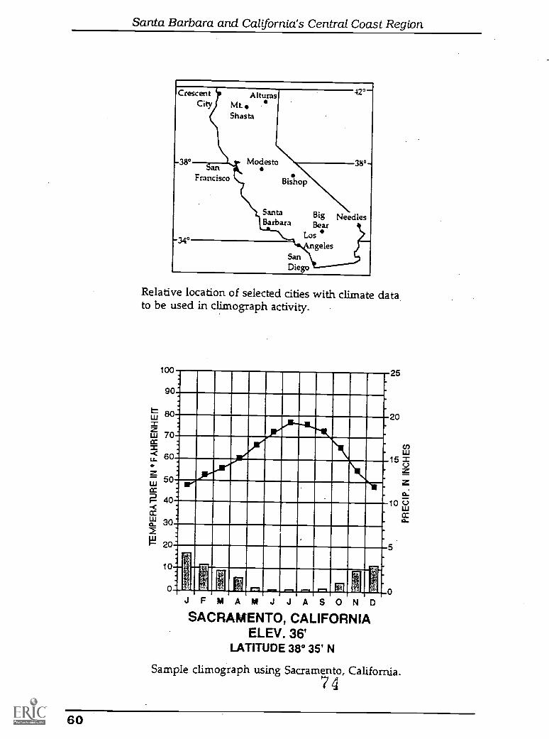
Santa Barbara and California's Central Coast Region
Crescent AlturasCity Mt.
Shasta
38° ModestoSan
Francisco
42°
Bishop
38°
SantaBig Needles
Barbara BearLos0
gelesSanDiego
Relative location of selected cities with climate datato be used in climograph activity.
100
90
so
70
60
50:
40
25
20
J F M A M J J A S O N D
SACRAMENTO, CALIFORNIAELEV. 36'
LATITUDE 38° 35' N
5
0
Sample climograph using Sacramento, California.74
60
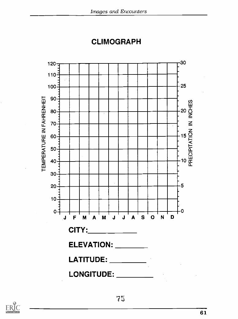
Images and Encounters
120
110
100
90
80
70
60
50
40
30
20
10
CLIMOGRAPH
0
MI
]
FMAMJCITY:
ELEVATION:
LATITUDE:
LONGITUDE:
J ASOND
30
25
u)w=20 0zzz
15 g_i--Ia_
010 i
wxa_
5
0
61
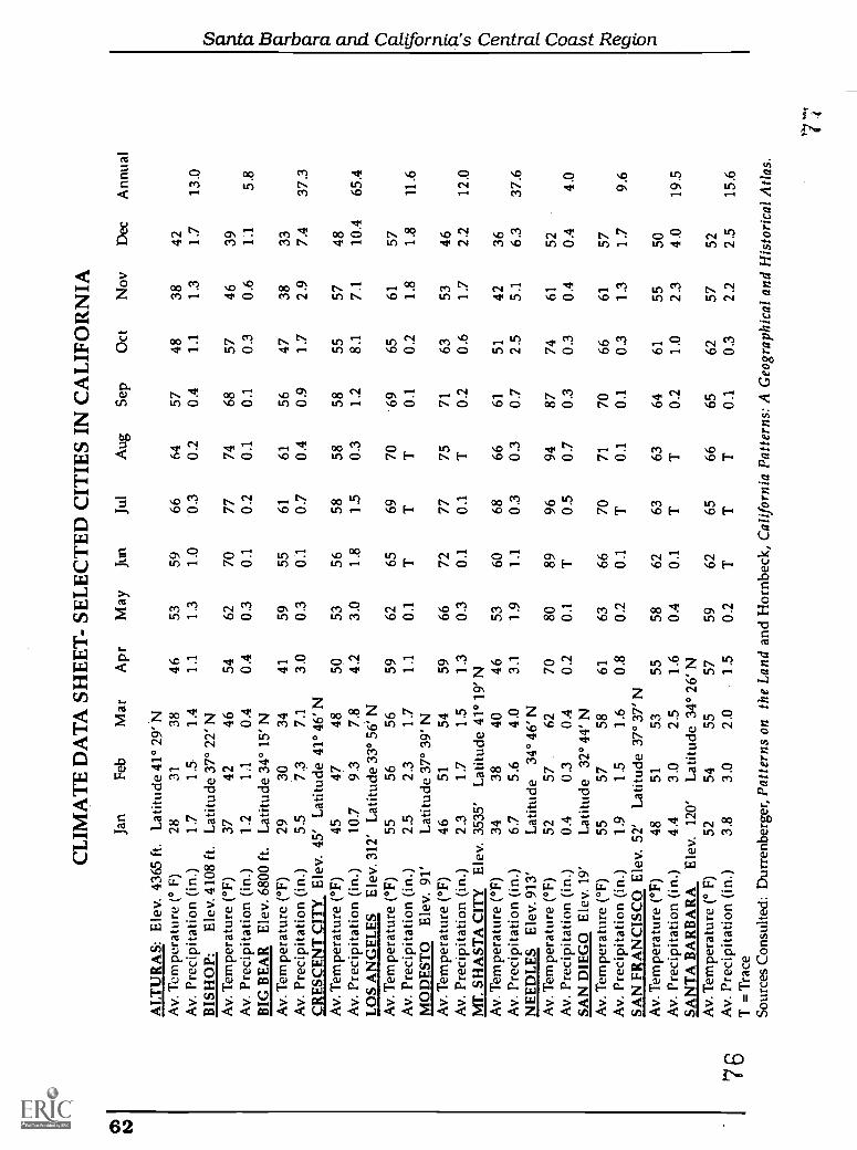
CL
IMA
TE
DA
TA
SH
EE
T-
SEL
EC
TE
D C
ITIE
S IN
CA
LIF
OR
NIA
AL
TU
RA
S: E
lev.
436
5 ft
.A
v. T
empe
ratu
re (
° F)
Av.
Pre
cipi
tatio
n (i
n.)
BIS
HO
P:E
lev.
410
8 ft
.A
v. T
empe
ratu
re (
°F)
Av.
Pre
cipi
tatio
n (i
n.)
BIG
BE
AR
Ele
v. 6
800
ft.
Av.
Tem
pera
ture
(°F
)A
v. P
reci
pita
tion
(in.
)
Jan
Feb
Mar
Apr
May
Jun
Jul
Aug
Sep
Oct
Nov
Dec
Ann
ual
Lat
itude
41°
29'
N28
3138
4653
5966
6457
4838
421.
71.
51.
41.
11.
31.
00.
30.
20.
41.
11.
31.
713
.0L
atitu
de 3
7° 2
2' N
3742
4654
6270
7774
6857
4639
1.2
1.1
0.4
0.4
0.3
0.1
0.2
0.1
0.1
0.3
0.6
1.1
5.8
Lat
itude
34°
15'
N29
3034
4159
5561
6156
4738
335.
57.
37.
13.
00.
30.
10.
70.
40.
91.
72.
97.
437
3C
RE
SCE
NT
CIT
Y E
lev.
45'
Lat
itude
41°
46'
NA
v. T
empe
ratu
re (
°F)
4547
4850
5356
5858
5855
5748
Av.
Pre
cipi
tatio
n (i
n.)
10.7
9.3
7.8
4.2
3.0
1.8
1.5
0.3
1.2
8.1
7.1
10.4
65.4
LO
S A
NG
EL
ES
Ele
v. 3
12' L
atitu
de 3
3° 5
6' N
Av.
Tem
pera
ture
(°F
)55
5656
59A
v. P
reci
pita
tion
(in.
)2.
52.
31.
71.
1M
OD
EST
O E
lev.
91'
Lat
itude
37°
39'
NA
v. T
empe
ratu
re (
°F)
4651
5459
Av.
Pre
cipi
tatio
n (i
n.)
2.3
1.7
1.5
1.3
MT
. SH
AST
A C
ITY
Ele
v. 3
535'
Lat
itude
41°
19'
NA
v. T
empe
ratu
re (
°F)
3438
4046
5360
6866
6151
4236
Av.
Pre
cipi
tatio
n (i
n.)
6.7
5.6
4.0
3.1
1.9
1.1
0.3
0.3
0.7
2.5
5.1
6.3
37.6
NE
ED
LE
S E
lev.
913
'L
atitu
de34
° 46
' NA
v. T
empe
ratu
re (
°F)
5257
6270
8089
9694
8774
6152
Av.
Pre
cipi
tatio
n (i
n.)
0.4
0.3
0.4
0.2
0.1
T0.
50.
70.
30.
30.
40.
44.
0SA
N D
IEG
O E
lev.
19'
Lat
itude
32°
44'
NA
v. T
empe
ratu
re (
°F)
5557
5861
6366
7071
7066
6157
Av.
Pre
cipi
tatio
n (i
n.)
1.9
1.5
1.6
0.8
0.2
0.1
T0.
10.
10.
31.
31.
79.
6SA
N F
RA
NC
ISC
O E
lev.
52'
Lat
itude
37°
37'
NA
v. T
empe
ratu
re (
°F)
4851
5355
5862
6363
6461
5550
Av.
Pre
cipi
tatio
n (i
n.)
4.4
3.0
2.5
1.6
0.4
0.1
TT
0.2
1.0
2.3
4.0
19.5
SAN
TA
BA
RB
AR
AE
lev.
120
'L
atitu
de 3
4° 2
6' N
Av.
Tem
pera
ture
(°
F)52
5455
5759
6265
6665
6257
52A
v. P
reci
pita
tion
(in.
)3.
83.
02.
01.
50.
2T
TT
0.1
0.3
2.2
2.5
15.6
T =
Tra
ceSo
urce
s C
onsu
lted:
Dur
renb
erge
r, P
atte
rns
on th
e L
and
and
Hor
nbec
k, C
alif
orni
a Pa
ttern
s: A
Geo
grap
hica
l and
His
tori
cal A
tlas.
6265
6970
6965
6157
0.1
TT
T0.
10.
21.
81.
811
.6
6672
7775
7163
5346
0.3
0.1
0.1
T0.
20.
61.
72.
212
.0
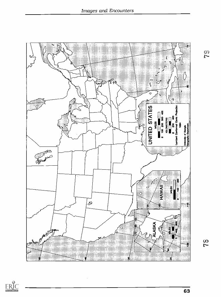
78
MIL
ES
=IC
C]
010
0 20
0 30
0 40
0K
ILO
ME
TE
RS 1
020
040
0La
mbe
rt C
onfo
rmal
Con
ic P
ro *
Jo:
1994
'7$
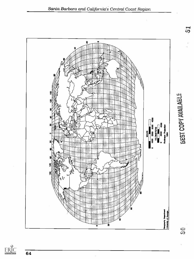
Santa Barbara and California's Central Coast Region
64
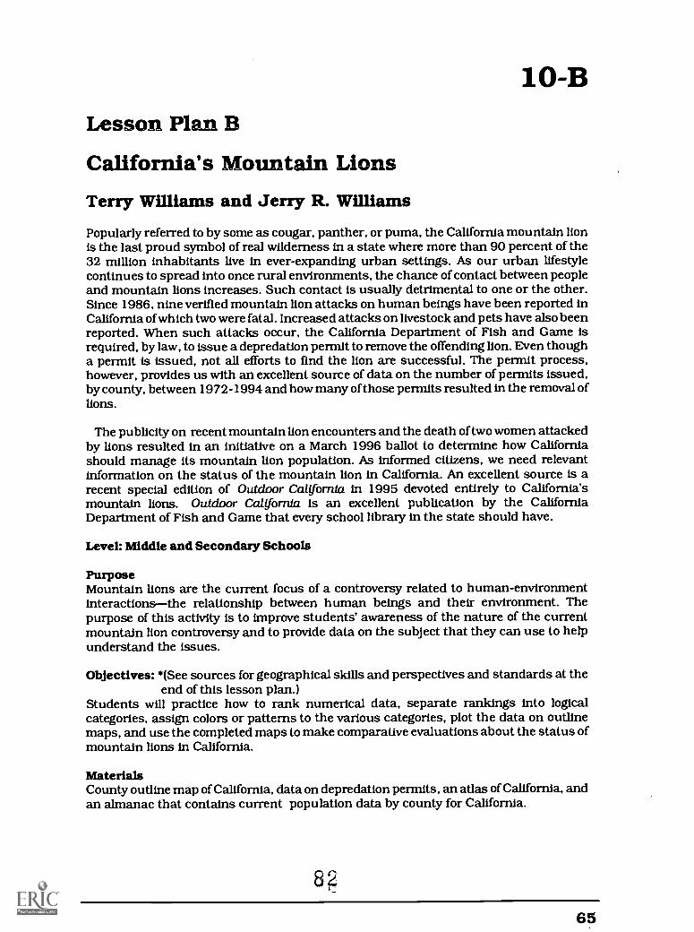
10-BLesson Plan B
California's Mountain LionsTerry Williams and Jerry R. Williams
Popularly referred to by some as cougar, panther, or puma, the California mountain lionis the last proud symbol of real wilderness in a state where more than 90 percent of the32 million inhabitants live in ever-expanding urban settings. As our urban lifestylecontinues to spread into once rural environments, the chance of contact between peopleand mountain lions increases. Such contact is usually detrimental to one or the other.Since 1986, nine verified mountain lion attacks on human beings have been reported inCalifornia of which two were fatal. Increased attacks on livestock and pets have also beenreported. When such attacks occur, the California Department of Fish and Game isrequired, by law, to issue a depredation permit to remove the offending Hon. Even thougha permit is issued, not all efforts to find the lion are successful. The permit process,however, provides us with an excellent source of data on the number of permits issued,by county, between 1972-1994 and how many of those permits resulted in the removal oflions.
The publicity on recent mountain lion encounters and the death of two women attackedby lions resulted in an initiative on a March 1996 ballot to determine how Californiashould manage its mountain lion population. As informed citizens, we need relevantinformation on the status of the mountain lion in California. An excellent source is arecent special edition of Outdoor California in 1995 devoted entirely to California'smountain lions. Outdoor California is an excellent publication by the CaliforniaDepartment of Fish and Game that every school library in the state should have.
Level: Middle and Secondary Schools
PurposeMountain lions are the current focus of a controversy related to human-environmentinteractionsthe relationship between human beings and their environment. Thepurpose of this activity is to improve students' awareness of the nature of the currentmountain lion controversy and to provide data on the subject that they can use to helpunderstand the issues.
Objectives: *(See sources for geographical skills and perspectives and standards at theend of this lesson plan.)
Students will practice how to rank numerical data, separate rankings into logicalcategories, assign colors or patterns to the various categories, plot the data on outlinemaps, and use the completed maps to make comparative evaluations about the status ofmountain lions in California.
MaterialsCounty outline map of California, data on depredation permits, an atlas of California, andan almanac that contains current population data by county for California.
65
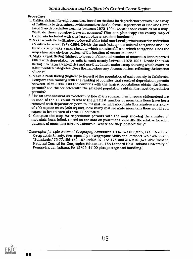
Santa Barbara and California's Central Coast Region
Procedure1. California has fifty-eight counties. Based on the data for depredation permits, use a map
of California to determine in which counties the California Department of Fish and Gameissued no depredation permits between 1972-1994. Locate those counties on a map.What do those counties have in common? (You can photocopy the county map ofCalifornia included with this lesson plan as student handouts.)
2. Make a rank listing (highest to lowest) of the total number of permits issued in individualcounties between 1972-1994. Divide the rank listing into natural categories and usethese data to make a map showing which counties fall into which categories. Does themap show any obvious pattern of the location of mountain lions?
3. Make a rank listing (highest to lowest) of the total number of mountain lions reportedkilled with depredation permits in each county between 1972-1994. Divide the ranklisting into natural categories and use that data to make a map showing which countiesfall into which categories. Does the map show any obvious pattern reflecting the locationof lions?
4. Make a rank listing (highest to lowest) of the population of each county in California.Compare this ranking with the ranking of counties that received depredation permitsbetween 1972-1994. Did the counties with the largest populations obtain the fewestpermits? Did the counties with the smallest populations obtain the most depredationpermits?
5. Use an almanac or atlas to determine how many square miles (or square kilometers) arein each of the 11 counties where the greatest number of mountain lions have beenremoved with depredation permits. If a mature male mountain lion requires a territoryof 100 square miles (259 sq tan), how many mature male mountain lions would youexpect to live in each of these 11 counties?
6. Compare the map for depredation permits with the map showing the number ofmountain lions killed. Based on the data on your maps, describe the relative locationpatterns of mountain lions in California. Where are they located? Why?
*Geography for Life: National Geography Standards 1994. Washington, D.C.: NationalGeographic Society. See especially : "Geographic Skills and Perspectives," 49-55 and"Standards," 75-77,156-159, 197 and 96-97, 173-175, and 214-215. (Available from theNational Council for Geographic Education, 16A Leonard Hall, Indiana University ofPennsylvania, Indiana, PA 15705, $7.00 plus postage and handling.)
83
66
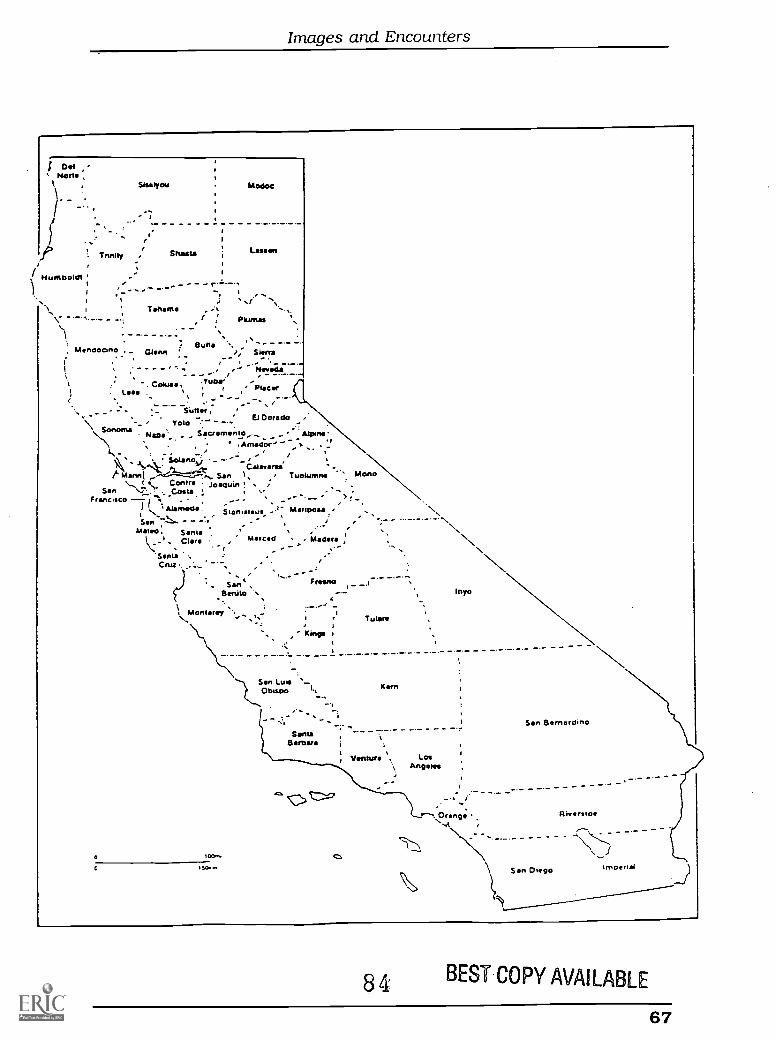
Images and Encounters
Ps tilos' Modoe
-'1
)
...
1' I
I
,/:' Inn Ily : Shasta i Lassen
i ;Humboldt '
I
1 i1 ....
\ I Tatum'... '
'.\ . - -._ - - ..,,...
.% Bun' ,.. - - -*- -
Mendocino - _ Ghmn ; ) Sierra. . . .. - .1 , ' - - ---I - Nevada
1
, Plumes
-.me
Coluaa ,.
*Yuba'e -'' Placer
1La . .
,r , -
\r
_..' El Dorado ..
Naos facramonio,._ Alpine- .
\ . nmadoe' /i.... - . ... '-k ........,.. ,., -Solana.' -.- ,
Calmer's,.
__-__ __.2---...eat
14 0Aanitt --..*----;'--"..... San 1, TUOIUMIN ..'. Mono
San -..., .. Costs e. , ,\-...C. Contra Joaquin ! . ; . -... -Francisco I re. . , ,- ,
,.J ',. ' Alamedai s. ,,..
Suirualus --'. lAllnPaml '_ .. - , '
San 7,-...- -, e, ,e
Mato° e Santa -.1-
,.. .' Merced .. Madan' ,''..... Clara .
'Santa ., .. . .
s
-._ _.-,c Fresno _.j_ San ; -
Benito 'S 14-
Monterey a
a Tulare
0 106
Kings I
San Lute s-.Obispo Kern
-Santa
earners
Ventura 1, LosAnginas
N.N
lnyo
. Orange
San Bernardino
San Diego ImDerug
84 BEST CM AVAILABLE
67
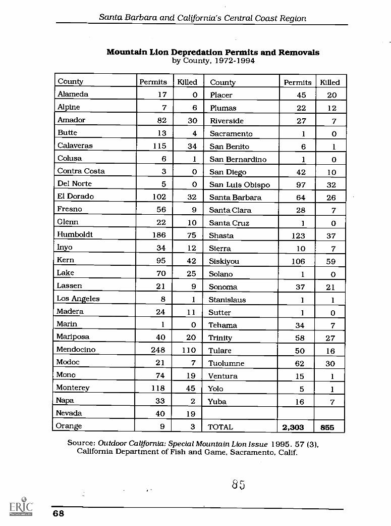
Santa Barbara and California's Central Coast Region
Mountain Lion Depredation Permits and Removalsby County, 1972-1994
County Permits Killed County Permits Killed
Alameda 17 0 Placer 45 20Alpine 7 6 Plumas 22 12
Amador 82 30 Riverside 27 7Butte 13 4 Sacramento 1 0Calaveras 115 34 San Benito 6 1
Colusa 6 1 San Bernardino 1 0Contra Costa 3 0 San Diego 42 10Del Norte 5 0 San Luis Obispo 97 32El Dorado 102 32 Santa Barbara 64 26Fresno 56 9 Santa Clara 28 7Glenn 22 10 Santa Cruz 1 0Humboldt 186 75 Shasta 123 37Inyo 34 12 Sierra 10 7Kern 95 42 Siskiyou 106 59Lake 70 25 Solari() 1 0Lassen 21 9 Sonoma 37 21Los Angeles 8 1 Stanislaus 1 1
Madera 24 11 Sutter 1 0Marin 1 0 Tehama 34 7Mariposa 40 20 Trinity 58 27Mendocino 248 110 Tulare 50 16Modoc 21 7 Tuolumne 62 30Mono 74 19 Ventura 15 1
Monterey 118 45 Yolo 5 1
Napa 33 2 Yuba 16 7Nevada 40 19
Orange 9 3 TOTAL 2,303 855
Source: Outdoor California: Special Mountain Lion Issue 1995. 57 (3),California Department of Fish and Game, Sacramento, Calif.
65
68
10-CLesson Plan C
Water and the California Landscape:A Geographical PerspectiveTerry Wil lams and Jerry R. Williams
IntroductionThe availability of water has always been of concern in California and, as the population ofthe state continues to grow, the concern over the continued availability of water grows withit. Climatically speaking, much of California has a semi-arid or desert environment. Inaddition, annual precipitation is concentrated in a few winter months and in the northernpart of the state.
Level: Middle and Secondary School
Objective : (See sources on geographical skills and perspectives and standards at the endof this lesson.)
To demonstrate how the people of California have compensated for the seasonal andlocational characteristics of precipitation and, in the process, created a unique water-oriented landscape.
MaterialsThis activity lends itself to students working in teams of two with laminated desk maps ofthe state. You can also use a wall map of California or handout base maps of the state.**
Water For AgricultureThe long hot summers of California are ideal for growing crops. In addition to hot weather,however, farmers need water to make the crops grow. California has developed a number ofwater transfer projects during the twentieth century. One of the first was in the ImperialValley in southern California.
1. The Imperial Valley is a desert, seldom receiving 5" of precipitation a year with slightlylarger amounts received during the winter than the summer.
2. The growing season in the Imperial Valley ranges from 275 to 335 days.3. The Colorado River carries runoff from the Rocky Mountains through the southwestern
United States, along the southern border of California into Mexico and eventually to theGulf of California.a. Much of the Imperial Valley lies below sea level. In the 1890s, local landowners decidedto dig ditches from the Colorado River to the valley to provide a much needed sourceofwater.b. In 1905, a major flood occurred on the Colorado River and the entire river broke throughthe natural levees and followed the course of the new irrigation ditches into the ImperialValley. The break was not filled until 1907 and the river was diverted back into its naturalchannel. The flood waters from the Colorado River created a huge lake in the ImperialValley known as the Salton Sea.c. Today the Salton Sea covers about 360 square miles (829 sq km). Circle the Salton Seaon your map and write HUMAN- MADE SEA next to it.
4. After the Colorado River was diverted back into its old channel, a new canal, The All
69
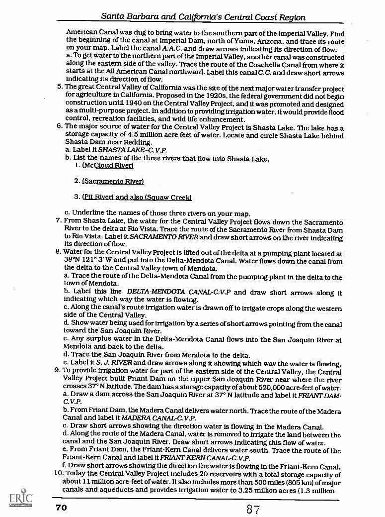
Santa Barbara and California's Central Coast Region
American Canal was dug to bring water to the southern part of the Imperial Valley. Findthe beginning of the canal at Imperial Dam, north of Yuma, Arizona, and trace its routeon your map. Label the canal A.A.C. and draw arrows indicating its direction of flow.a. To get water to the northern part of the Imperial Valley, another canal was constructedalong the eastern side of the valley. Trace the route of the Coachella Canal from where itstarts at the All American Canal northward. Label this canal C.C. and draw short arrowsindicating its direction of flow.
5. The great Central Valley of Californiawas the site of the next major water transfer projectfor agriculture in California. Proposed in the 1920s, the federal government did not beginconstruction until 1940 on the Central Valley Project, and itwas promoted and designedas a multi-purpose project. In addition to providing irrigation water, it would provide floodcontrol, recreation facilities, and wild life enhancement.
6. The major source of water for the Central Valley Project is Shasta Lake. The lake has astorage capacity of 4.5 million acre feet of water. Locate and circle Shasta Lake behindShasta Dam near Redding.a. Label it SHASTA LAKE-C.V.'?b. List the names of the three rivers that flow into Shasta Lake.
1. (McCloud River)
2. fSacramento River)
3. (pit River) and also (Squaw Creek)
c. Underline the names of those three rivers on your map.7. From Shasta Lake, the water for the Central Valley Project flows down the Sacramento
River to the delta at Rio Vista. Trace the route of the Sacramento River from Shasta Damto Rio Vista. Label it SACRAMENTO RIVER and draw short arrows on the river indicatingits direction of flow.
8. Water for the Central Valley Project is lifted out of the delta at a pumping plant located at38°N 121° 3' W and put into the Delta-Mendota Canal. Water flows down the canal fromthe delta to the Central Valley town of Mendota.a. Trace the route of the Delta-Mendota Canal from the pumping plant in the delta to thetown of Mendota.b. Label this line DELTA-MENDOTA CANAL-C.V.P and draw short arrows along itindicating which way the water is flowing.c. Along the canal's route irrigation water is drawn off to irrigate crops along the westernside of the Central Valley.d. Show water being used for irrigation by a series of short arrows pointing from the canaltoward the San Joaquin River.c. Any surplus water in the Delta-Mendota Canal flows into the San Joaquin River atMendota and back to the delta.d. Trace the San Joaquin River from Mendota to the delta.e. Label it S. J. RIVER and draw arrows along it showing which way the water is flowing.
9. To provide irrigation water for part of the eastern side of the Central Valley, the CentralValley Project built Friant Dam on the upper San Joaquin Rivernear where the rivercrosses 37° N latitude. The dam has a storage capacity of about 520,000 acre-feet of water.a. Draw a dam across the San Joaquin River at 37° N latitude and label it FRIANT DAM-C.V.P.b. From Friant Dam, the Madera Canal delivers water north. Trace the route of the MaderaCanal and label it MADERA CANAL-C.V.P.c. Draw short arrows showing the direction water is flowing in the Madera Canal.d. Along the route of the Madera Canal, water is removed to irrigate the land between thecanal and the San Joaquin River. Draw short arrows indicating this flow of water.e. From Friant Dam, the Friant-Kern Canal delivers water south. Trace the route of theFriant-Kern Canal and label it FRIANT-KERN CANAL-C.V.P.f. Draw short arrows showing the direction the water is flowing in the Friant-Kern Canal.
10. Today the Central Valley Project includes 20 reservoirs with a total storage capacity ofabout 11 million acre-feet of water. It also includes more than 500 miles (805 km) of majorcanals and aqueducts and provides irrigation water to 3.25 million acres (1.3 million
70 87
Santa Barbara and California's Central Coast Region
hectares) of agricultural land.11. As California continued to grow, new plans were developed to transfer more water
within the state. In the 1960s, the state undertook a massive new project, the CaliforniaWater Project.a. The primary water storage area for the California WaterProject is Orovllle Lake. It hasa storage capacity of about 3.5 million acre-feetof water. Locate and cirde Oroville Lake,about 100 miles (160 km) north of the state capital.b. Label it OROVILLE LAKE-C.W.P.c. Name the major rivers that flow into Oroville Lake.(Feather River-North Fork, Feather River-Mid Fork and Feather River-South Fork)
12. From Oroville Lake, the water for the California Water Project flows in the Feather Riveruntil it empties into the Sacramento River north of the city of Sacramento. Trace thecourse of the Feather River and label it FEATHERRIVER-C.W.P.
13. After it flows into the Sacramento River, water for the California Water Project flows intothe delta to a huge pumping plant next to the Delta-Mendota Canal pumping plant. Atthe pumping plant water is lifted up into the California Aqueduct and begins its journeysouth.a. Trace a line along the aqueduct to the San Luis Reservoir and label it CALIFORNIAAQUEDUCT-C.W.P.b. Draw short arrows along the route of the CaliforniaAqueduct indicatingthe directionthe water is flowing.c. The San Luis Reservoir (southwest of Merced) is a storage place for excess water fromOroville Lake. It can store about two million acre-feet of water. Circle itand label it SANLUIS RESERVOIR-C.W.P.d. From San Luis Reservoir, the aqueduct continues south to the end of the CentralValley near 35° N 119° W. Trace a line along the aqueduct's route to this point.e. Label it CALIFORNIA AQUEDUCT-C.W.P. and draw short arrows indicating thedirection the water is flowing in the aqueduct.
14. At the southern end of the Central Valley, water in the CaliforniaAqueduct is pumpedup and over the Tehachapi Mountains and into southern California where it finallyends at a reservoir near Moreno Valley (east of Riverside).a. Trace the remainder of the route of the California Aqueduct.b. Label itCALIFORNIAAQUEDUCT-C.W.P.c. Draw short arrows indicating the direction the water in the aqueduct is flowing.
This activity gives an overall impression of how the California landscape has beenchanged in the process of making use of the state's water resources to satisfy the needsof the inhabitants. It also illustrates changes in technology. The earlier Central ValleyProject. with the one exception of lifting the water initially into the Delta-Mendota Canal,relies on gravity flow to move the water. The use of arrows in the exercise illustrates howthe engineers were able to take advantage of the natural topography to facilitate the flowof water. In contrast, the later California Water Project uses massive amounts of energyto pump the water. Although the systems in this exercise are critical to Californiaagriculture, the California Water Project also provides water for urban uses, as do anumber of other major projects not included in this activity.
Since the last major water project was initiated in California. the size of the state'spopulation has grown by approximately ten million people. Where willthe water supply forthe state's increasing population come from? How might people modify the landscape inthe future to meet those needs? Those topics lend themselves to important discussionsthat will affect the lives of all the inhabitants of this state in the future. For example, whatare the advantages and disadvantages of each of the following alternatives?
1. New water projectsa. Are there any other major sources of water in the state that have not already been
used?b. Is water that is allowed to flow to the sea really being wasted?c. What happens if we drill more wells and try to make more intensive use of ground
water?
8S 71
Santa Barbara and California's Central Coast Region
d. Is the- available ground water close enough to the demand, or will it also have to betransported?
e. Is desalinization of ocean water a viable water supply alternative for major urbancenters in the immediate future?
2. Can we transfer water to California from Washington, Alaska, or Canada, as some peoplesuggest, to solve our water needs?a. What are the implications of such massive water transfer systems?b. Is it feasible to tow icebergs from Antarctica to the coast of California to supply :our
needs?3. Is conservation and more efficient use of existing water supplies the answer to our water
needs?4. How do we balance the environmental needs for water with our urban and commercial
needs?5. Are there other alternatives?
References and Sources
* Geography for Life: National Geography Standards 1994. Washington, D.C.: NationalGeographic Society. See especially pp. 46-56 for "Skills and Perspectives" and pp. 92-95,96-97 for 'Standards." (Available from the National Council for Geographic Education,16A Leonard Hall, Indiana University of Pennsylvania, Indiana, PA 15705, $7.00 pluspostage and handling)
**The Department of Water Resources and the Water Education Foundation each has a largeCalifornia water map that provides an excellent overview of water delivery systems inCalifornia. A Water Project Facilities in California map is included at the end of this lesson.
8S
72
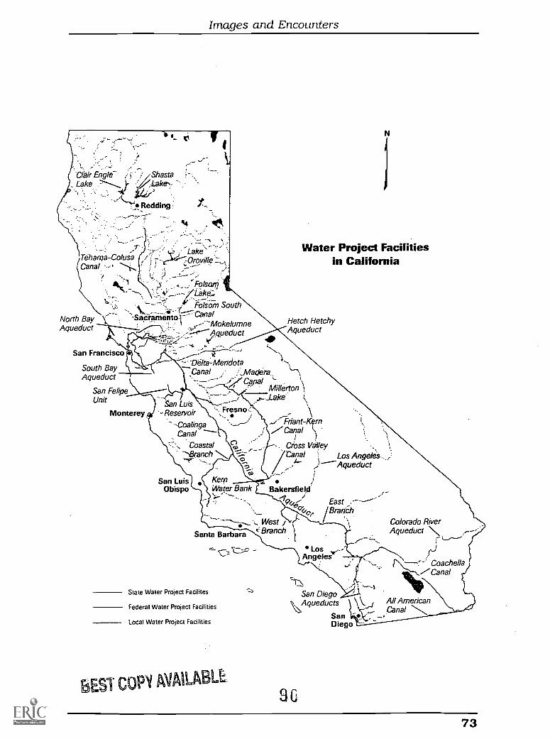
Images and Encounters
Clair Engle-. Lake
/ShastaLake-
Redding
44
. -
Teharpa-ColuSa.Canal
North Bay acrarnentof"Aqueduct
Lake'.
San Francisco
South BayAqueduct
San FelipeUnit
Monterey
EST C
FolsomLake;
Folsom SouthCanal,--'-`Mokelumne
Aqueduct
--Delta-MendotaCanal
qPPal Millerton
\Fr/ant-Kern
7' Canal
. Cross Vdiley'Canal
Aqueduct
Bakersfield'-9 East
'Bran&I
Water Project Facilitiesin California
Hatch HetchyAqueduct
an Luis- Reservoir
-CoalingaCanal
Coastal-",Branch\
Fresno.
San LuisObispo
KernWater Bank
Santa Barbara
State Water Project Facilites
Federal Water Project Facilities
Local Water Project Facilities
PY AVAILABLE
1
Los Angelis-...;
- West /Branch
Los v.--Angeles
San Diegot. Aqueducts
9 C
SanDiego
Colorado RiverAqueduct \
,P)Coachella
lcCanal
kAll AmericanCanal
73
10-DLesson Plan D
The Travels of a MonarchCarol Douglass
Through aeons of time, the approach of winter in North America has initiated a naturalphenomenon that has become the delight of both children and adults. In the autumn,countless thousands of Monarch butterflies leave Canada and the northern United Statesand fly to Mexico or California, where they spend the winter. In early spring, adults mateand begin their j ourney back north, with females laying eggs along the way. The distributionand density of Monarch butterfly populations is regulated by the common milkweed plant;it provides nectar for the adult butterfly, a depository for eggs, and a food source for the larvaor caterpillar stage of the butterfly. The eggs hatch, metamorphose, and a new butterflyjoins the on-going migration.
The Monarch butterfly, Danaus plexippus, is an ideal insect for students of all ages tostudy. By observing the transformations involved in insect metamorphosis, mapping theirdistribution in other lands, tracing their migratory routes in North America, writing andillustrating a story about their life cycle, or calculating the distance they travel from Canadato Mexico, Monarch butterflies can provide the focus for an integrative approach to science,geography, language arts, art, and mathematics.
Level: Elementary and Middle Schools
PurposeTo learn about the migration of the Monarch butterfly.
Objectives: (See sources for geographic skills and perspectives and standards inGeography for Life, noted with the sources at the end of this lesson.)
To trace the geographical routes of the Monarch butterfly from Canada to Mexico and fromthe northwestern United States to California using landforms and map symbols.
MaterialsWall map of North America.Laminated desk maps or paper outline maps of North America (included at the end ofthis lesson). Story of the Monarch's journey.Pictures of landforms for reference.
ActivityFollow the journey of the Monarchs from Canada to Mexico or from the northwestern UnitedStates to California, using terms that refer to landforms, states, and directions. Acondensed version of the journey would include:
Story of the Monarch's JourneyCanada to MexicoSome Monarchs began their life cycle near Highland Creek, Toronto, Canada. As theystarted their migration south in September, they encountered rain and wind as theycrossed southern Lake Ontario; they soon came to an open field and continued to flysouthward over northern Lake Erie. As they flew across Pennsylvania, the country becamehilly and in West Virginia they crossed over the forested Appalachian Mountains. By
91
74
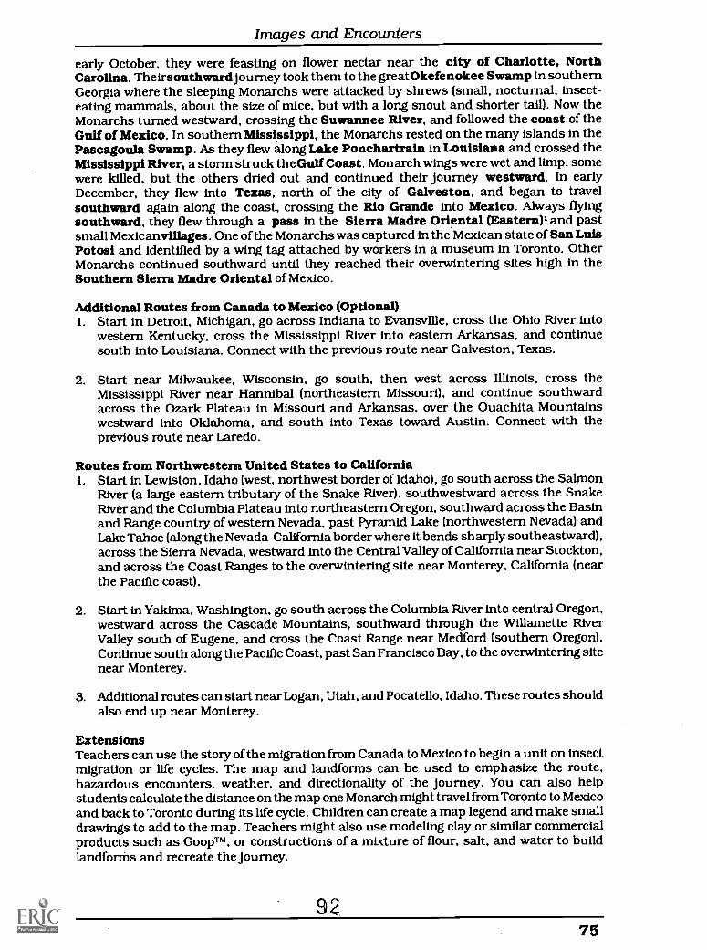
Images and Encounters
early October, they were feasting on flower nectar near the city of Charlotte, NorthCarolina. Theirsouthward journey took them to the great Okefenokee Swamp in southernGeorgia where the sleeping Monarchs were attacked by shrews (small, nocturnal, insect-eating mammals, about the size of mice, but with a long snout and shorter tail). Now theMonarchs turned westward, crossing the Suwannee River, and followed the coast of theGulf of Mexico. In southern Mississippi, the Monarchs rested on the many islands in thePascagoula Swamp. As they flew along Lake Ponchartrain in Louisiana and crossed theMississippi River, a storm struck the Gulf Coast. Monarch wings were wet and limp, somewere killed, but the others dried out and continued their journey westward. In earlyDecember, they flew into Texas, north of the city of Galveston, and began to travelsouthward again along the coast, crossing the Rio Grande into Mexico. Always flyingsouthward, they flew through a pass in the Sierra Madre Oriental (Eastern)1 and pastsmall Mexicanvillages. One of the Monarchs was captured in the Mexican state of San LuisPotosi and identified by a wing tag attached by workers in a museum in Toronto. OtherMonarchs continued southward until they reached their overwintering sites high in theSouthern Sierra Madre Oriental of Mexico.
Additional Routes from Canada to Mexico (Optional)1. Start in Detroit, Michigan, go across Indiana to Evansville, cross the Ohio River into
western Kentucky, cross the Mississippi River into eastern Arkansas, and continuesouth into Louisiana. Connect with the previous route near Galveston, Texas.
2. Start near Milwaukee, Wisconsin, go south, then west across Illinois, cross theMississippi River near Hannibal (northeastern Missouri), and continue southwardacross the Ozark Plateau in Missouri and Arkansas, over the Ouachita Mountainswestward into Oklahoma, and south into Texas toward Austin. Connect with theprevious route near Laredo.
Routes from Northwestern United States to California1. Start in Lewiston, Idaho (west, northwest border of Idaho), go south across the Salmon
River (a large eastern tributary of the Snake River), southwestward across the SnakeRiver and the Columbia Plateau into northeastern Oregon, southward across the Basinand Range country of western Nevada, past Pyramid Lake (northwestern Nevada) andLake Tahoe (along the Nevada-California border where it bends sharply southeastward),across the Sierra Nevada, westward into the Central Valley of California near Stockton,and across the Coast Ranges to the overwintering site near Monterey, California (nearthe Pacific coast).
2. Start in Yakima, Washington, go south across the Columbia River into central Oregon,westward across the Cascade Mountains, southward through the Willamette RiverValley south of Eugene, and cross the Coast Range near Medford (southern Oregon).Continue south along the Pacific Coast, past San Francisco Bay, to the overwintering sitenear Monterey.
3. Additional routes can start near Logan, Utah, and Pocatello, Idaho. These routes shouldalso end up near Monterey.
ExtensionsTeachers can use the story of the migration from Canada to Mexico to begin a unit on insectmigration or life cycles. The map and landforms can be used to emphasize the route,hazardous encounters, weather, and directionality of the journey. You can also helpstudents calculate the distance on the map one Monarch might travel from Toronto to Mexicoand back to Toronto during its life cycle. Children can create a map legend and make smalldrawings to add to the map. Teachers might also use modeling clay or similar commercialproducts such as GoopTM, or constructions of a mixture of flour, salt, and water to buildlandfonns and recreate the journey.
9275
Santa Barbara and California's Central Coast RegionSourcesHitchins, Ross 1966. The Travels of Monarch X. Chicago, Ill.: Rand McNally, 1966.
Mudd, Maria M. 1991. The Butterfly, Dimensional Nature Portfolio Series. NewYork: Stewart,Tabori, and Chang (Contains a beautiful, three-dimensional Monarch butterfly).
"My Mexican Monarchs," Ranger Rick, October 1991.
Geography for Life: National Geography Standards 1994. Washington, D.C.: NationalGeographic Society. "Skills and Perspectives" 46-52; "Standards" 120-121, 158-159;132-133, 171-172; and 136-137, 176-178. (Available from the National Council forGeographic Education, 16A Leonard Hall, Indiana University of Pennsylvania, Indiana,PA 15705, $7.00 plus postage and handling.)
Urquhart, Fred A. 1976. "Found at Last: The Monarch's Winter Home."National Geographic150 (August) 161-173.
1987. The Monarch Butterfly: International Traveler. Chicago: Nelson-Hall.(The authoritative work on the Monarchan excellent source.)
Sierra means mountains or mountain range in Spanish and oriental means eastern. Theeastern mountains of the high Plateau of Mexico are called the Sierra Madre Oriental andwestern mountains along the Plateau of Mexico are called the Sierra Madre Occidental (occidentalis Spanish for western). Where the western coast of southern Mexico trends southeastward, theSierra Madre Occidental become the Sierra Madre del Sur (sur is Spanish for south).
93.
76
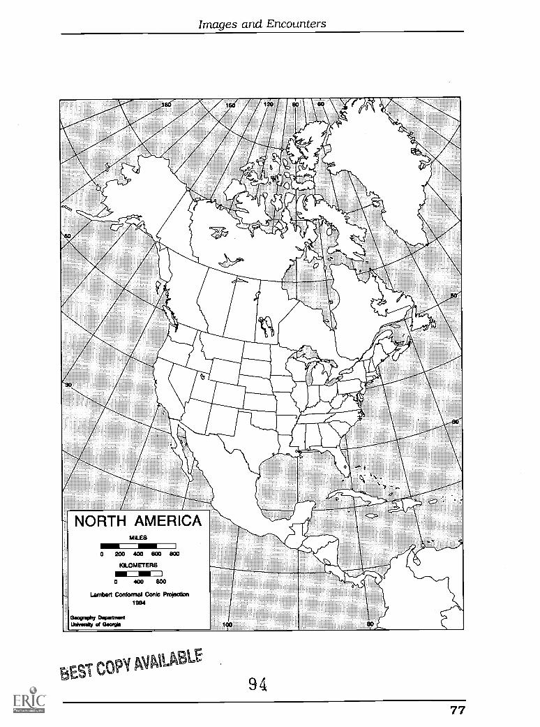
Images and Encounters
BESTCOPY AVAILABLE
9.77
10-ELesson Plan E
Rice: A World FoodEunice Gavin
Several thousand years ago, somewhere in southeast Asia, rice was gradually transformedfrom a wild grass to a domesticated grain-producing plant. Today one of the several thousandvarieties of rice that now exist can be found growing on every continent except Antarctica.The cultivation of rice ranges from the deserts of Egypt to the slash-and-burn agriculture ofthe Amazon Basin and everywhere in between. Rice is a major food source for half of theworld's population. Although the United States produces only about one percent of the totalworld production, it accounts for 18 percent of all rice exports. Incontrast to most of the restof the world, where rice production is highly labor-intensive, rice production in the UnitedStates is highly mechanized and capital-intensive.
Level: Elementary and Middle Schools
PurposeThis lesson will introduce students to the history and cultivation of rice and focus on riceproduction in California. Using a piece of children's literature, this lesson will also examinethe cultural diversity of a neighborhood and highlight a food that is common to each of theculturesrice.
Objectives: (See Geography for 4e for geographical skills and perspectives and standardslisted at the end of this lesson.)Students will identify the rice producing regions of California, the UnitedStates, and theworld.Students will acquire knowledge about rice production in California.Students will identify the geographic location of the families mentioned in the literature.
MaterialsA copy of the book, Everybody Cooks Riceby Norah Dooley (Minneapolis: Carolrhoda Books1991).A world desk map for every two students (master supplied in Lesson Plan A).An outline map of California and the United States (supplied in Lesson Plans A and B). Acopy of the pamphlet, Facts About USA Rice, for each student (see how to procure this underreferences at the end of this lesson).
ProcedureRicePart I1. Skim the history article in Facts about USA Rice to find the importance of the following
dates in U. S. History-1726, 1849, 1884, and 1920.2. Find and outline South Carolina on the U.S. map. Write inside South Carolina "1726-
4,500 Metric Tons of Rice Exported."3. On the U.S. map, find and outline, as one region, the states of Missouri, Arkansas,
Louisiana, Mississippi, and Texas. Inside the region write "1884Beginning of MajorU. S. Rice Production."
95
78
Images and Encounters
4. Find California on the U.S. map. Write "1849-40,000 Chinese Inhabitants and1920Major U.S. Rice Producer."
5. Find Florida on the U.S. map. Outline the state and write "Newest Rice-ProducingState."
6. Rice is grown in 14 counties throughout California's Central Valley. However, theprimary rice growing region lies north of Sacramento in the counties of Butte,Colusa, Glenn, Sacramento, Sutter, Tehama, Yolo, and Yuba. Shade in those countieson a California map.
7. As the second largest producer of rice in the United States, after Arkansas, Californiaaccounts for about 20 percent of all rice grown in this country. California rice growersproduce the highest average annual yield, i.e., production per unit area, of rice per acre(or per hectare) in the world. Approximately 392,000 acres (158,700 hectares) of land aredevoted to rice production in California. There are 640 acres in one square mile (or 259hectares). Calculate how many square miles of agricultural land are used to produce ricein this state. (A little more than 600 square miles-- 612.5 sq. mi. or 1586 sq km.)
8. All of the land devoted to rice production in California is about equal to the total land areaof one of the rice-producing counties. Use an almanac or an atlas to determine the area,in square miles, of each of the major rice-producing counties. Identify which county ismost equal in size to the total land devoted to rice growing in California. Draw an arrowpointing to that county and label it "Approximate Area Used to Grow Rice." (Sutter-607 sq. mi. or 1572 sq km; Yuba-639 sq. mi. or 1655 sq km)
9. Climate, soil, and water are major physical factors influencing rice production. Examinethe map and an atlas to see what the eight counties listed above have in common thatmake them a major rice producing region.
10. Read the article on cultivation and discuss how rice farming today is different from ricefarming long ago and how it differs in the U.S. from manyother countries. What is theprocedure for growing rice?
RicePart II1. Read the story, Everybody Cooks Rice, to the class.2. On a world desk map, locate the country of origin of each family mentioned in the story.
Put an X on each country (Barbados, Puerto Rico, Vietnam, India, China, and Haiti).3. Discuss similarities of the families in the story with families typical of many California
communities.4. As a class project, compile a list of all the different types of food with which the students
are familiar that contain rice.
RicePart III1. Skim the history article in Facts about USA Rice to find the first recorded account of rice
cultivation.2. Find and outline China on the world map. Write "2,800 B.C.lst Documented
AcCount of Rice Planting" across the country of China. Based on the written record,determine how many years rice has been grown in China (at least 4,795 yearsprobably5,000 years).
3. Today, rice is a staple crop for much of the world's population. Most of the rice is eatenin the countries where it is grown. Ask the students to identify the countries, they think,are the top ten rice-producers in the world today. Based on their discussion, record theirchoices on the board.
4. Identify the top ten rice-producing countries and compare these to the class list.Students should locate the countries on their world map and underline the country'sname. Draw a rice grain for each 10 million tons produced next to each country listed onthe following table.
5. After they have located the countries, students should draw in the appropriate numbersof grains of rice on each of the top ten rice-producing countries.
96,79
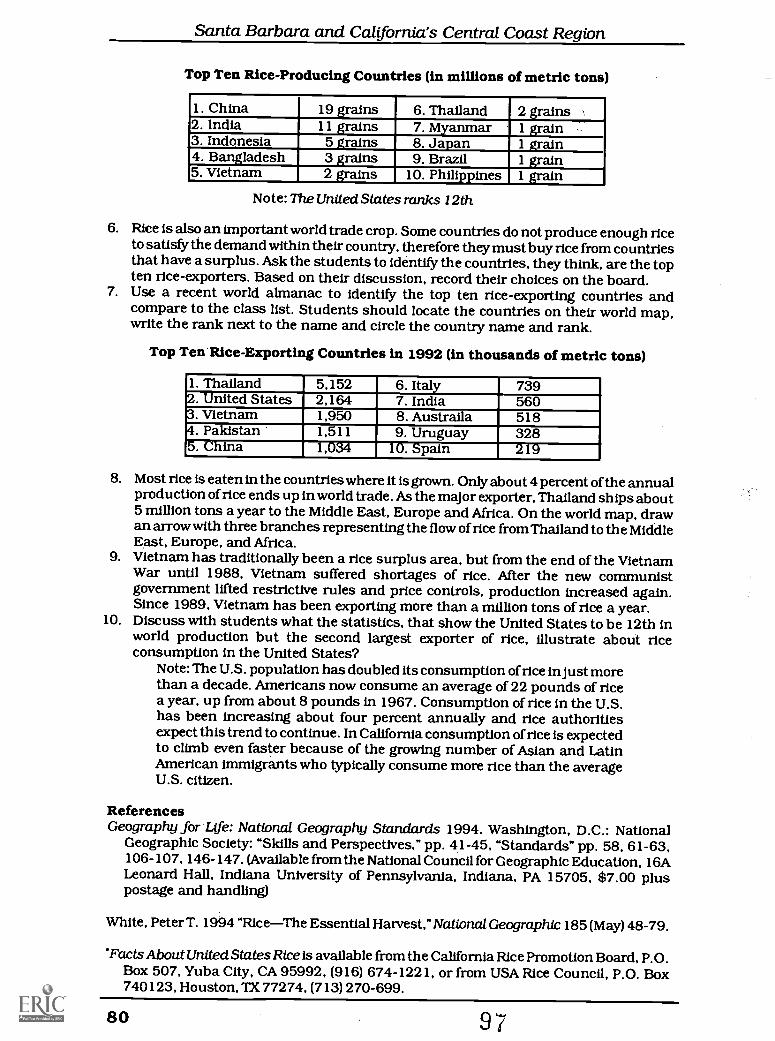
Santa Barbara and California's Central Coast Region
Top Ten Rice-Producing Countries (In millions of metric tons)
1. China 19 grains 6. Thailand 2 grains s.
2. India 11 grains 7. Myanmar 1 grain3. Indonesia 5 grains 8. Japan 1 grain4. Bangladesh 3 grains 9. Brazil 1 grain5. Vietnam 2 grains 10. Philippines 1 grain
Note: The United States ranks 12th
6. Rice is also an important world trade crop. Some countries do not produce enough riceto satisfy the demand within their country, therefore they must buy rice from countriesthat have a surplus. Ask the students to identify the countries, they think, are the topten rice-exporters. Based on their discussion, record their choices on the board.
7. Use a recent world almanac to identify the top ten rice-exporting countries andcompare to the class list. Students should locate the countries on their world map,write the rank next to the name and circle the country name and rank.
Top Ten Rice-Exporting Countries in 1992 (in thousands of metric tons)
1. Thailand 5,152 6. Italy 7392. United States 2,164 7. India 5603. Vietnam 1,950 8. Australia 5184. Pakistan 1,511 9. Uruguay 3285. China 1,034 10. Spain 219
8. Most rice is eaten in the countries where it is grown. Only about 4 percent of the annualproduction of rice ends up in world trade. As the major exporter, Thailand ships about5 million tons a year to the Middle East, Europe and Africa. On the worldmap, drawan arrow with three branches representing the flow of rice from Thailand to the MiddleEast, Europe, and Africa.
9. Vietnam has traditionally been a rice surplus area, but from the end of the VietnamWar until 1988, Vietnam suffered shortages of rice. After the new communistgovernment lifted restrictive rules and price controls, production increased again.Since 1989, Vietnam has been exporting more than a million tons of rice a year.
10. Discuss with students what the statistics, that show the United States to be 12th inworld production but the second largest exporter of rice, illustrate about riceconsumption in the United States?
Note: The U.S. population has doubled its consumption of rice in justmorethan a decade. Americans now consume an average of 22 pounds of ricea year, up from about 8 pounds in 1967. Consumption of rice in the U.S.has been increasing about four percent annually and rice authoritiesexpect this trend to continue. In California consumption of rice is expectedto climb even faster because of the growing number of Asian and LatinAmerican immigrants who typically consume more rice than the averageU.S. citizen.
ReferencesGeography for Life: National Geography Standards 1994. Washington, D.C.: National
Geographic Society: "Skills and Perspectives," pp. 41-45, "Standards" pp. 58, 61-63,106-107, 146-147. (Available from the National Council for Geographic Education, 16ALeonard Hall, Indiana University of Pennsylvania, Indiana, PA 15705, $7.00 pluspostage and handling)
White, Peter T. 1994 "Rice-The Essential Harvest,"National Geographic 185 (May) 48-79.
'Facts About United States Rice is available from the California Rice Promotion Board, P.O.Box 507, Yuba City, CA 95992, (916) 674-1221, or from USA Rice Council, P.O. Box740123, Houston, 'IX 77274, (713) 270-699.
80 97

NOTES
98 BEST COPY AVAILABLE
(9/92)
e
U.S. DEPARTMENT OF EDUCATIONOffice of Educational Research and Improvement (OEM
Educational Resources Information Center (ERIC)
NOTICE
REPRODUCTION BASIS
ERIC
This document is covered by a signed "Reproduction Release(Blanket)" form (on file within the ERIC system), encompassing allor classes of documents from its source organization and, therefore,does not require a "Specific Document" Release form.
This document is Federally-funded, or carries its own permission toreproduce, or is otherwise in the public domain and, therefore, maybe reproduced by ERIC without a signed Reproduction Releaseform (either "Specific Document" or "Blanket").