POLITICS OR MOBILITY? EVIDENCE FROM US EXCISE TAXATION

Alejandro Esteller-Moré, Leonzio Rizzo

Document de treball de l’IEB 2010/3

Fiscal Federalism

Documents de Treball de l’IEB 2010/3

POLITICS OR MOBILITY? EVIDENCE FROM US EXCISE TAXATION

Alejandro Esteller-Moré, Leonzio Rizzo The IEB research program in Fiscal Federalism aims at promoting research in the public finance issues that arise in decentralized countries. Special emphasis is put on applied research and on work that tries to shed light on policy-design issues. Research that is particularly policy-relevant from a Spanish perspective is given special consideration. Disseminating research findings to a broader audience is also an aim of the program. The program enjoys the support from the IEB-Foundation and the IEB-UB Chair in Fiscal Federalism funded by Fundación ICO, Instituto de Estudios Fiscales and Institut d’Estudis Autonòmics. The Barcelona Institute of Economics (IEB) is a research centre at the University of Barcelona which specializes in the field of applied economics. Through the IEB-Foundation, several private institutions (Caixa Catalunya, Abertis, La Caixa, Gas Natural and Applus) support several research programs. Postal Address: Institut d’Economia de Barcelona Facultat d’Economia i Empresa Universitat de Barcelona C/ Tinent Coronel Valenzuela, 1-11 (08034) Barcelona, Spain Tel.: + 34 93 403 46 46 Fax: + 34 93 403 98 32 ieb@ub.edu http://www.ieb.ub.edu The IEB working papers represent ongoing research that is circulated to encourage discussion and has not undergone a peer review process. Any opinions expressed here are those of the author(s) and not those of IEB.

Documents de Treball de l’IEB 2010/3

POLITICS OR MOBILITY?

EVIDENCE FROM US EXCISE TAXATION *

Alejandro Esteller-Moré, Leonzio Rizzo ABSTRACT: We test for the state interdependence of gasoline and cigarette taxation in the US (1975-2006). We estimate a tax reaction function, and find that state interdependence is due solely to yardstick competition, since any interaction disappears completely in the case of states with lame duck governors. This result holds for both taxes: the short-run reaction of those states whose governor is eligible to stand for reelection is 0.13 and 0.21 for gasoline and cigarette taxation, respectively. In the long run, the cigarette tax rates levied in a jurisdiction match those of its neighbors perfectly, while the long-run reaction in the case of gasoline is much lower at 0.72. JEL Codes: H71, H77

Keywords: Tax competition, political accountability, excise taxes.

Alejandro Esteller-Moré Universitat de Barcelona & IEB Dep. d'Economia Política i Hisenda Pública Facultat d'Economia i Empresa Av. Diagonal, 690 08034 Barcelona (Spain) E-mail: aesteller@ub.edu

Leonzio Rizzo Università di Ferrara & IEB Department of Economics Via Voltapaletto, 11 44100 Ferrara (Italy) E-mail: leonzio.rizzo@unife.it

* We are grateful for bilateral funding from the Italian and Spanish governments (“Acción Integrada HI2007-0094”), from the UB (“Projectes pre-competitius, Modalitat A”), from the Generalitat de Catalunya (2009SGR102), and from the Ministerio de Ciencia e Innovación (ECO2009-12928).

1. Introduction There can be little doubt that US excise tax rates are state interdependent (Nelson, 2002;

Rork, 2003; Devereux, Lockwood and Redoano, 2007; Jacobs, Ligthart and Vrijburg,

2010). All previous studies, despite obvious differences in their empirical analyses,

report a positive tax reaction to neighbors’ tax rates, and implicitly or explicitly argue

that such a response is caused by strategic tax competition attributable to cross-border

shopping, smuggling or both. In this paper we focus on taxes on cigarettes and gasoline

in the US and show that tax interdependence is due solely to tax mimicking.

Brueckner (2003) describes two sources of strategic interaction among governments,

captured in the resource-flow and spillover models respectively. The former stresses the

role of tax base mobility, while the latter points to the possibility of information spilling

over among interested voters in different jurisdictions (Salmon, 1987). Unfortunately, it

is difficult in practice to disentangle one source from the other, as both models make the

same empirical prediction, namely that tax rates should be interdependent among sub-

central governments. In the case of tax competition, tax base mobility is required; in the

case of yardstick competition, it is assumed that voters assess the relative performance

of their respective governments and compare it with that of comparable governments

when deciding who to cast their vote for. Thus, for this accountability mechanism to

work, fiscal information must be readily available to voters.

In order to disentangle tax competition from that of yardstick, we proceed as Besley and

Case (1995a). We distinguish those states run by a governor who is ineligible to run for

reelection (because of a term limit) from all other states. We test their differential

reaction for cigarette and gasoline taxes for a panel dataset running from 1975 to 2006.

We find that only those governors who are not lame ducks set their tax rates by taking

into account the rates levied by comparable jurisdictions - which, in keeping with the

literature (see, for example, Besley and Case, 1995a), we shall from this point on

identify as the geographically contiguous states - while the other governors set taxes

independently of the behavior of their neighbors. Specifically, in the case of governors

not approaching the end of their tenure, a one-cent increase in the real tax rate of their

neighbors implies a contemporaneous tax increase of 0.13c and 0.21c for gasoline and

cigarettes, respectively; moreover, in the long run a one-cent increase will be perfectly

2

matched in the case of cigarettes, while in the case of gasoline it will rise to 0.72c.

Therefore, in spite of a fairly well-documented tax base mobility, it does not seem to be

the cause of the average tax interdependence among US states in the case of excise

taxation. Rather, states tend to mimic each other because of their reelection concerns

regarding the role of excise taxation.

The rest of the paper is organized as follows. In the next section, we provide a summary

of the empirical literature on tax interdependence, focusing on yardstick competition

and on the analyses carried out for US excise taxation. In section three, we present the

empirical analysis and discuss the results. Finally, we conclude.

2. Previous literature

Salmon (1987) was the first author to recognize that comparative performance

constituted a potential source of fiscal interdependence among sub-national

governments. In his words, “each government has an incentive to do better than

governments in other jurisdictions in terms of levels and qualities of services, of levels

of taxes or of more general economic and social indicators” (p. 32). Subsequently,

Besley and Case (1995a) developed a sophisticated information externality model

among jurisdictions. The model implies that voters draw on relevant information from

comparable jurisdictions in order to infer fiscal information that is fundamental in

helping them make their next voting decision. Should this indeed be the case, then

politicians need to be well aware of what their comparable jurisdictions are doing if they

wish to ensure their own reelection for a further term.

Besley and Case (1995a) tested this hypothesis by comparing the tax-setting decisions

of those governors that could be reelected with the rates chosen by those who could not.

They tested it both for state income-tax liability and for an amalgam of state taxes

(sales, income and corporate income), and in both cases found that lame duck governors

did not make tax changes that were dependent on their neighbors’ rates, which was very

much in contrast with the performance of the rest of the state governors. If tax

competition were the cause of tax interdependence, then the reaction should have been

independent of whether governors could be held accountable (no term limit) or not

(binding term limit). For this reason, the authors conclude that the tax interdependence

3

found was due only to yardstick competition. In more recent studies, this source of tax

interdependence has also been found by Bordignon, Cerniglia and Revelli (2003), Solé-

Ollé (2003), and Allers and Elhorst (2005). All of which were undertaken with local

governments in various countries with a primary focus on property taxation.

In the case of excise taxation, there is considerable empirical evidence of tax

interdependence for the US case. However, as a result no doubt of the extensive

anecdotic evidence that cross-border shopping, and even smuggling, are very important

in certain areas, authors have tended not to devote much time in attempting to

disentangle the most likely source of this interdependence.

Rork (2003) reported a horizontal reaction of 0.636 and 0.6 cents for cigarette and

gasoline, respectively. He measured each tax in (real) cents, and attributed all the

reaction to tax base mobility. However, if state taxes are serially correlated (which is the

case for excise taxes, since statutory tax rates do not often vary over time) and the

empirical specification fails to take this into full account, the estimates might be

upwardly biased. In order to tackle this problem, Devereux, Lockwood and Redoano

(2007), and Jacobs, Ligthart and Vrijburg (2010) include the lagged endogenous

variable with the result that the estimate of the horizontal reaction is considerably lower.

The former obtain a reaction of 0.277 and 0.191 (though, statistically insignificant) for

cigarette and gasoline taxation, respectively. Jacobs, Ligthart and Vrijburg (2010)

define the tax rate variable as an “average effective tax rate”, which is an average of the

state sales tax and specific tax rates. In their case, and although not fully comparable

with the two previous results, the reaction they estimate is around 0.4. Yet, in both

analyses the presence of the lagged endogenous variable allows them to obtain a long-

run reaction, which is almost equal to 1.

While Jacobs, Ligthart and Vrijburg (2010) remain silent about the source of tax

interdependence, Devereux, Lockwood and Redoano (2007) suggest that their results

point to tax competition as being the most likely source, since in their spatial lag model

the average of all the rest of state taxes is not statistically significant while the tax

average constructed using neighbor weights works better. However, note that their

conclusions might be somewhat hastily drawn, as information externalities are usually

thought to flow more easily between neighboring jurisdictions (Salmon, 1987; Besley

4

and Case, 1995a).

In contrast with these previous studies, and now that the presence of tax

interdependence is well documented, we aim at identifying the source of this

interdependence. Our results are clear-cut and robust: tax interdependence in excise

taxation is due solely to yardstick competition.

3. Empirical analysis

3.1. Empirical framework

To test for the source of horizontal tax interaction in the US, we estimate the tax-

reaction function by relating one state tax to the average tax of its neighboring states for

the period 1975-2006. We then repeat this procedure for gasoline and cigarette taxes

transformed into real terms (using the federal CPI).

In order to estimate the potentially different reaction of states depending on whether

their governor can or cannot stand for reelection, we estimate the following equation for

each case:

jstjstjstsi

jstsii

jstsitsjst tXtwtwt εμβϕϕφα ++++++= −≠

− ∑∑ 11' [1]

where jstt is the real tax rate on commodity j for state s in year t; sα is a state fixed

effect; tφ is a year effect; ∑≠ si

jstsitw is the average real tax rate for commodity j of the

neighboring states of state s in year t, where siw are identical exogenous weights,

normalized such that ∑≠

=si

si 1ω , which account for the relative interdependence relation

between s and the rest of the i-states; jstX is a vector of state-specific time-varying

regressors; while jstε is a mean zero, normally distributed random error. As long as the

estimate of ϕϕ +' is different from zero for the sample where the governor is not a lame

duck and equal to zero for the sample where the governor is a lame duck, we can

confirm that the interaction is solely the result of yardstick competition. If ϕ were to be

5

significant in both samples, then tax competition would be operative, but if yardstick

competition were also present , we would expect a lower estimate for lame duck

governors.

In Besley and Case (1995a), but also in Case (1993), “… the empirical specification

[will] use changes in taxes as the main tax-setting decision. Such changes are most

likely to represent responses to shocks about which there is asymmetric information” (p.

32). While tax levels have been used elsewhere (e.g., Solé-Ollé, 2003; and Allers and

Elhorst, 2005), here we opt for a more parsimonious empirical specification. We include

the lagged endogenous variable and a lag of the neighbors’ tax in a model that

constitutes a general version of Besley and Case’s (1995a) empirical specification. As

long as the estimate of the lagged endogenous variable is equal to 1, and the (absolute

value of the) estimate of the contemporaneous and lagged neighbors’ tax rate is equal,

our model collapses into theirs. Thus, a priori our model does permit both types of

reaction: both in levels and changes.

In order to isolate the independent impact of the average of the neighboring states’ tax,

we include other variables that might affect the state tax rate and that must be taken into

account in order to avoid biased estimates. These variables are included in the

vector jstX . Specifically, state taxation may be influenced by the economic and

demographic environment. As is usual in the literature, this is controlled for by the

following variables: population (and its square), per-capita income (and its square),

unemployment rate, proportion of population over 65 and proportion of population

between 5 and 17. We also take federal fiscal instruments into account, as these may

differ from state to state and might condition the setting of state tax rates. Thus, we

include federal grants-in-aid in relation to total population and the federal income tax

collected in each state, normalized by the adjusted gross income. The political affiliation

of the state government may also affect the tax rate level. We build dummies for the

governors' party affiliation (Democrat or Republican) and variables to account for the

percentage representation of the political parties (Democrat or Republican) in the House

and in the Senate.

Certain invariable state characteristics are likely to affect its tax system, such as climate

6

or geography, among others. We take these characteristics into account by including a

dichotomous variable for each state. Changes in the macroeconomic situation may also

affect a state’s fiscal policies, and so we include a set of time effects.

The mean US neighboring tax rate,∑≠ si

jstsitw , is endogenous because it can be

simultaneously influenced by the tax rate that we are estimating. Then, if this was a

structural model, a simple OLS estimation of [1] would suffer from endogeneity bias:

the error term εjst would be correlated with the error terms of the other simultaneous

equations in the system. In order to overcome the simultaneity bias, we use the two-

stage least-squares method: first, we estimate the reduced forms of the endogenous

variables, and then we substitute their fitted values into [1]. The residuals of this last

equation are corrected using the actual values of the endogenous variables. We

instrument the mean US neighboring tax rate with the US neighboring variables POPst,

CHILDst, AGEDst, UNEMPst, DEMSENst, DEMHOUst. Consequently, we have six

instruments in total. Hence Equation [1], which has one endogenous variable, can be

identified.1

3. 2. Data

3.2.1 Nominal tax rates

Taxes on gasoline and cigarettes vary considerably across states. In 1990, for example,

the tax per pack of cigarettes ranged from 2 cents in North Carolina to 40 cents in

Connecticut. In the same year, the tax per gallon of gasoline ranged from 7.5 cents in

Georgia to 22 cents in Connecticut and Washington. Thus, there is significant cross-

sectional variation.

Individual state taxes on cigarettes also vary over time. For example, in North Carolina

the tax rate varied between 2 and 5 cents in 1992, but reached 30 cents in 2005 and 35

in 2006. Connecticut shows even more variation, levying a tax of 21 cents up to 1983,

before increasing the rate to 26 cents in 1984, then raising it again to 40 in 1989, 45 in

1 The lag of the dependent variable biases all the estimated coefficients of the regression for finite-T samples. However, in our case, the Nickell (1981) bias should not be a significant problem, due to the fact that our panel runs over 32 years. Therefore, we do not instrument the lagged endogenous variable.

7

1992, 47 in 1994, 50 in 1995, 111 in 2002 and finally 151 cents in 2003. Likewise,

individual state taxes on gasoline show considerable variation over time. While Georgia

maintained the same tax (7.5 cents) throughout the period studied here, the rate varied

markedly in Connecticut and Washington. Connecticut increased its tax rate from 10 to

11 cents per gallon in 1976, to 14 in 1983 and then to 38 in 1997. This was followed by

a reduction to 36 cents in 1998, 32 in 1999 and, finally, to 25 in 2002. Washington

levied 9 cents till 1976, which rose gradually to 18 in 1984, 22 in 1990 and 23 in 1991.

The tax was then increased to 28 in 2004, 31 in 2005 and, finally, 34 in 2006.

3.2.2 Description of the term limit variable

This is a dichotomous variable, but one that varies considerably by state and year in our

sample. There are states in which there is no term limit on the governor’s election;

while in others there is a one-term limit (Virginia), a two-term limit, or a three-term

limit (Utah). Additionally, some states in our sample have changed their legislation

from a no-term limit to a two-term limit or from a one-term limit to a two-term limit.

Besley and Case (1995b) and List and Sturm (2006) have exploited this variation

between states and over time in order to assess the potentially different performance of

lame duck governors.

3.2.3 The other variables

The rest of the right-hand-side variables in [1], with their definitions, averages and

standard deviations are reported in Table 1.

[TABLE 1]

We include a set of time-varying variables that characterize the states’ economic and

demographic situation: the state population (POP), per capita state income (INC), the

state unemployment rate (UNEMP), the proportion of individuals in the state who are

aged between 5 and 17 (CHILD), and the proportion who are over 65 (AGED). The

states’ political environment can also affect fiscal outcomes. Therefore, we use a

dummy variable that equals one if the governor is a Democrat (DEMGOV). We also

account for the proportion of Democrats in the state Senate and in the House of

Representatives (DEMSEN and DEMHOU, respectively). The cigarette and gasoline

industries might affect the state tax rate by lobbying for the rates of their respective

8

commodities (Dixit, 1996). Therefore, in order to control for the influence of lobbies,

we include TOBINC (tobacco production per dollar of state income) and GASINC

(gasoline production per dollar of state income). The federal fiscal policy, other than

commodity tax rates, may also affect state commodity tax rates. Thus, we control for

per capita federal grants to the states (GRANTS), and the average federal income in the

state (INCTAX), defined as the ratio of the state’s federal income tax liability to its

adjusted gross income.

3.3. Empirical results

In Table 2, we present our results for taxes on gasoline. In column (1), we estimate a

restricted model, as it only includes the contemporaneous value of the neighbors’ tax

variable. The short-run reaction is 0.226, while the long-run reaction is 1.121 (i.e.,

0.2263/(1-0.7982)). In column (2), we include a lag of the neighbors’ tax variable,

which is statistically significant. The short-run reaction is now slightly lower, 0.151

(i.e., 0.6605-0.5090), while the long-run reaction is 0.796. In Table 3, we obtain similar

results for taxes on cigarettes. When we estimate the most flexible model (lagged

endogenous variable and lagged tax competitors’ variable), the short- and long-run

reactions (see again column (2)) are 0.175 and 1.167, respectively. Therefore, in both

cases, in line with results published elsewhere in the literature, we find positive tax

interdependence, albeit somewhat higher in the case of cigarettes. However, recall, we

are interested in identifying the source of this interdependence.

[TABLE 2]

That is why, going back to gasoline, in Table 2, we distinguish those states whose

governor can run for reelection (column (3)) from those where there is a binding term

limit (column (4)). In this latter case, it is clear that the reaction is not statistically

significant, while in the case where the governor can run for reelection the short-run

reaction is 0.134 and the long-run reaction is 0.718. Therefore, as in Besley and Case

(1995a), the empirical evidence points to yardstick competition. Similarly, in Table 3,

we obtain the same qualitative results: lame duck governors do not react to neighboring

cigarette tax rates. In contrast (column (3)), the rest of the state governors, in the short

run, faced by a 1-cent increase in their neighbor’s cigarette tax rates, raise their tax rates

9

by 0.21c, while in the long-run the increase can be as high as 1.488 (which cannot be

rejected as it is not equal to 1).

[TABLE 3]

The long-run reaction, especially in the case of cigarette taxation, is quite high. For this

reason, in Table 4, we present a robustness check including lags of the neighbors’ tax

rates rather than the lagged dependent variable.2 The first three columns of Table 4 refer

to gasoline, while the rest refer to cigarettes. Note that in columns (1) and (4), we do not

distinguish according to whether a term limit is at work or not. However, in columns (3)

and (6) we do show the results for the lame duck governors, but the reaction is still

statistically insignificant. When the state governor is eligible to run for reelection

(column (2)), the long-run reaction in the case of gasoline is equal to 0.695, while in the

case of cigarettes (column (5)) the reaction is equal to 0.976. Hence, the qualitative

results do not change, but now the long-run reactions are slightly lower.

[TABLE 4]

Finally, in the next two tables, we deflate the nominal statutory tax rates by using a state

price index.3 Since a general price index disaggregated by states is not available for the

US, we use the Housing Price Index (HPI), which is readily available for our entire time

span.4 In Table 5 we present the results for gasoline and in Table 6 we do the same for

cigarette taxation. The structure of both tables is identical to that of Tables 2 and 3,

respectively. First, when not distinguishing between states according to the presence or

otherwise of a term limit, we still obtain positive reactions, although their values are

lower. Second, in the case of both cigarette and gasoline taxation rates, states only react 2 Chirinko and Wilson (2009) show that the standard lagged dependent variable model (i.e., the one we use) is nested within a more general dynamic model that does not include the lagged dependent variable but an infinite number of time lags of the independent variables. Note that we have estimated a restricted version of that more general model as we only include four lags of the neighbors’ tax rates and none for the remaining exogenous variables. 3 Lockwood and Migali (2008) use a country-retail price index to deflate statutory tax rates when they estimate tax interdependence in excise taxes for the EU. 4 In spite of the volatility of the housing market, Esteller and Rizzo (2009) show that this index performs quite well in estimating the deflated reaction functions for cigarettes and gasoline in the US.

10

when their governor can run for reelection. Hence, the qualitative results are also robust

to the deflator used to transform nominal tax rates in real terms. In the case of gasoline,

the reaction is 0.061 and 0.312 in the short- and long-run, respectively; while in the case

of cigarettes, these reactions are equal to 0.281 and 1.063 (which cannot be rejected as it

is not equal to 1).

[TABLE 5]

[TABLE 6]

4. Conclusions

We explore the causes of the state interdependence of cigarette and gasoline taxation in

the US, and provide empirical evidence that only those states whose governor can run

for reelection react to their neighbors’ tax rates. This paper contributes to the literature

on US excise taxation by showing that tax rates are interdependent because incumbent

governors set their taxes in accordance with the rates levied by their neighbors so as to

ensure their reelection. Our results complement those reported by Besley and Case

(1995a), who found empirical evidence of yardstick competition in the case of income

tax rates in the US.

This result is quite robust to different specifications. Interestingly, the reaction when

governors are not lame ducks is much higher in the case of cigarettes. Indeed in this

case we cannot even reject the possibility that in the long run tax rates are perfectly

matched between neighboring jurisdictions. We leave the explanation of this differential

behavior between gasoline and cigarette taxation for further research.

11

References Allers, M.A., J. P. Elhorst (2005): “Tax Mimicking and Yardstick Competition among Local Governments in the Netherlands”, International Tax and Public Finance, 12, 493-513. Besley, T., A.C. Case (1995a): “Incumbent Behavior: Vote-Seeking, Tax-Setting, and Yardstick Competition”, American Economic Review, 85, 25-45. Besley, T., A.C. Case (1995b): “Does Political Accountability Affect Economic Policy Choices? Evidence from Gubernatorial Term Limits”, Quarterly Journal of Economics, 110, 769-98.. Brueckner, J. K. (2003): “Strategic Interaction among Governments: An Overview of Empirical Studies”, International Regional Science Review, 26, 175-188. Case, A. (1993): “Interstate Tax Competition after TRA86”, Journal of Policy Analysis and Management, 12, 136-48. Chirinko, B., D. J. Wilson (2009): “Tax Competition among U.S. States: Racing to the Bottom or Riding on a Seesaw”, Federal Reserve of San Francisco, Working Paper 2008-03. Devereux, M.P., B. Lockwood, M. Redoano (2007): “Horizontal and vertical indirect tax competition: Theory and some evidence from the USA”, Journal of Public Economics, 91, 451-79. Dixit, A., (1996): “Special-interest lobbying and endogenous commodity taxation”, Eastern Economic Journal, 22, 375–388. Esteller, A., L. Rizzo (2009): “(Uncontrolled) Aggregate shocks or vertical tax interdependence? Evidence from gasoline and cigarettes”, Working Paper #24, Institut d’Economia de Barcelona. Jacobs, J.P.A.M., J. E. Ligthart, H. Vrijburg (2010): “Consumption tax competition among governments: Evidence from the United States”, International Tax and Public Finance, forthcoming. List, J. A., D. Sturm (2006): “How Elections Matter: Theory and Evidence from Environmental Policy,” Quarterly Journal of Economics, 121, 1249-1281. Lockwood, B., G. Migali (2008): “Did the Single Market Cause Competition in Excise Taxes? Evidence from EU Countries”, The Economic Journal, forthcoming. Nelson, M. A. (2002): “Using Excise Taxes to Finance State Government: Do Neighboring State Taxation Policy and Cross-Border Markets Matter?”, Journal of Regional Science, 42, 731-52.

12

Nickell, S. (1981): “Biases in dynamic models with fixed effects” Econometrica 49, 1417-1426. Rork, J. C. (2003): “Coveting Thy Neighbors’ Taxation”, National Tax Journal, 56, 775-87. Salmon, P. (1987): “Decentralisation as an Incentive Scheme”, Oxford Review of Economic Policy, 3, 24-43. Solé-Ollé, A. (2003): “Electoral accountability and tax mimicking: the effects of electoral margins, coalition government, and ideology”, European Journal of Political Economy, 19, 685-713.

13

Data Appendix

• tst US cigarette tax rate for state s in year t, divided by the CPI or the HPI. These rates are taken from www.OTPR.org: cigarette tax rates are expressed in US dollars per pack of 20 cigarettes and gasoline tax rates are expressed in US dollars per gallon of gasoline.

Endogenous variables

• ∑≠ si

stsitw is the mean of the states tax rates, divided by the CPI or HPI, of the

states bordering state s in year t. Demographic and economic variables

• POPst is the number of persons in state s in year t. This figure is taken from www.census.gov.

• CHILDst is the ratio of individuals aged 5-17 years to the total population of state s in year t, taken from www.census.gov for the USA.

• AGEDst is the ratio of individuals of over 65 years of age to the total population of state s in year t, taken from www.census.gov for the USA.

• UNEMPst is the unemployment rate for state s in year t, taken from www.stats.bls.gov.

• INCst is the per-capita income for state s in year t divided by the CPI or HPI. Income data were taken from http://www.bea.doc.gov.

• GRANTst is the per-capita federal grant-in-aid for state s in year t. It is obtained from "Federal Expenditures by State" which is part of the Consolidated Federal Funds Reports program from US Census Bureau.

• DEMGOVst dummy=1 if the governor of the state is a Democratic, taken from the Statistical Abstracts of the United States.

• TERMLIMITst dummy=1 if the governor cannot run for reelection, taken from the Statistical Abstracts of the United States.

• DEMSENst proportion of state Senate that is Democratic, taken from the Statistical Abstracts of the United States.

• DEMHOUst proportion of state House that is Democratic, taken from the Statistical Abstracts of the United States.

• CPIt (Consumer Price Index) was taken from the Statistical Abstracts of the United States (2000).

• HPIst (House Price Index) was taken from http://www.ofheo.gov, the website of the Office of Federal Housing Enterprise Oversight in the USA.

• TOBINCst annual tobacco production (thousand of pounds); from http://www.nass.usda.gov, the website of the National Agricultural Statistics Service in the USA.

• GASINCst is the daily gasoline production (thousand barrels per day) per dollar of state income in real terms with CPI or HPI; from http://www.eia.doe.gov, the website of the Energy Information Administration in the USA.

• INCTAXst federal income tax divided by adjusted gross income. Federal income tax and adjusted gross income are from the http://www.irs.gov, the website of the Internal Revenue Service, a Department of the Treasury in the USA.

14

Table 1: 'Summary statistics*

Variable Obs Mean Stand. Dev. Min Max

tg*10 (state unit gasoline tax, cents in real terms with CPI) 1504 121.487 27.700 37.202 236.760Tg*10 (federal unit gasoline tax cents in real terms with CPI) 1504 89.653 23.241 41.451 127.336tc*10 (state unit cigarette tax, cents in real terms with CPI) 1504 216.776 164.998 13.587 1302.276Tc*10 (federal unita cigarette tax cents in real terms with CPI) 1504 151.423 33.508 82.902 216.787tg*10 (state unit gasoline tax, cents in real terms with HPI) 1504 97.673 31.177 18.201 201.350Tg*10 (federal unit gasoline tax cents in real terms with HPI) 1504 74.898 25.379 31.025 147.409tc*10 (state unit cigarette tax, cents in real terms with HPI) 1504 160.183 89.162 7.990 649.710Tc*10 (federal unita cigarette tax cents in real terms with HPI) 1504 119.973 33.349 50.480 235.863Termlimit 1504 0.261 0.439 0 1GDP (real national gross domestic product , billion of dolllars in real terms with CPI) 1504 45.662 10.138 30.452 65.707GDP (real national gross domestic product , billion of dolllars in real terms with HPI) 1504 36.121 9.925 15.484 66.492FED UNEMP (federal unemployment rate) 1504 6.284 1.410 4 9.7DEF (federal deficit over national gross domestic product) 1504 0.026 0.020 -0.027 0.059

POP(state population*10-6) 1504 5.314 5.577 0.382 36.250INC (state income per capita*10-3 in real terms with CPI) 1504 140.754 28.405 78.134 251.798INC (state income per capita*10-3 in real terms with HPI) 1504 110.134 22.616 58.685 197.910UNEMP (state unemployment rate) 1504 5.984 2.018 2.3 17.4CHILD (proportion of population between 5 and 17) 1504 0.196 0.021 0.155 0.268AGED (proportion of population over 65) 1504 0.122 0.019 0.073 0.185TOBINC (tobacco production per dollar of state income in real terms with CPI) 1504 257.890 925.431 0 10225.09TOBINC (tobacco production per dollar of state income in real terms with HPI) 1504 323.134 1155.657 0 13393.34GASINC (daily gasoline production per dollar of state income in real terms with CPI) 1504 0.818 2.703 0.000 31.343GASINC (daily gasoline production per dollar of state income in real terms with HPI) 1504 0.950 3.211 0.000 35.934GRANTS (federal grants per capita in dollars*10-8 in real terms with CPI) 1504 563*10-8 226*10-8 231*10-8 2740*10-8

GRANTS (federal grants per capita in dollars*10-8 in real terms with HPI) 1504 444*10-8 199*10-8 151*10-8 2210*10-8

INCTAX (federal income tax divided by adjusted gross income) 1504 0.137 0.016 0.092 0.193DEMGOV (=1 if the governor is a Democrat) 1504 0.537 0.499 0 1DEMSEN (proportion of state Senate that is Democratic) 1504 0.577 0.186 0.086 1DEMHOU (proportion of state House that is Democratic) 1504 0.574 0.179 0.129 1*Figures are based on annual data for continental US states for the year 1975 to 2006, inclusive. All the monetary variables are espressed in real terms, divideded bythe Consumer Price Index (CPI) 1982-84 taken from the Statistical Abstract of the United States or the Housing Price Index (HPI) 1980 taken from the Office ofFederal Housing Enterprise Oversight (http://www.ofheo.gov). We do not include non continental states (Hawaii, District of Columbia and Alaska) and Nebraska,whose Legislature is unicameral and non-partisan.

15

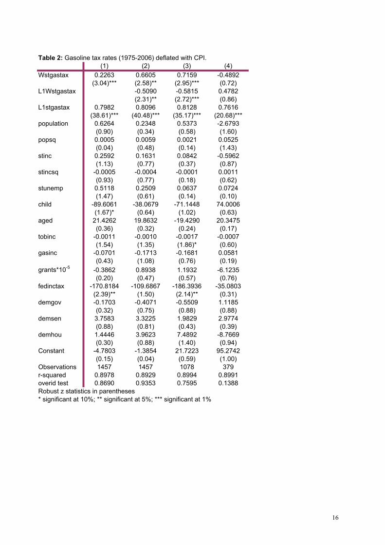
Table 2: Gasoline tax rates (1975-2006) deflated with CPI.(1) (2) (3) (4)

Wstgastax 0.2263 0.6605 0.7159 -0.4892(3.04)*** (2.58)** (2.95)*** (0.72)

L1Wstgastax -0.5090 -0.5815 0.4782(2.31)** (2.72)*** (0.86)

L1stgastax 0.7982 0.8096 0.8128 0.7616(38.61)*** (40.48)*** (35.17)*** (20.68)***

population 0.6264 0.2348 0.5373 -2.6793(0.90) (0.34) (0.58) (1.60)

popsq 0.0005 0.0059 0.0021 0.0525(0.04) (0.48) (0.14) (1.43)

stinc 0.2592 0.1631 0.0842 -0.5962(1.13) (0.77) (0.37) (0.87)

stincsq -0.0005 -0.0004 -0.0001 0.0011(0.93) (0.77) (0.18) (0.62)

stunemp 0.5118 0.2509 0.0637 0.0724(1.47) (0.61) (0.14) (0.10)

child -89.6061 -38.0679 -71.1448 74.0006(1.67)* (0.64) (1.02) (0.63)

aged 21.4262 19.8632 -19.4290 20.3475(0.36) (0.32) (0.24) (0.17)

tobinc -0.0011 -0.0010 -0.0017 -0.0007(1.54) (1.35) (1.86)* (0.60)

gasinc -0.0701 -0.1713 -0.1681 0.0581(0.43) (1.08) (0.76) (0.19)

grants*10-5 -0.3862 0.8938 1.1932 -6.1235(0.20) (0.47) (0.57) (0.76)

fedinctax -170.8184 -109.6867 -186.3936 -35.0803(2.39)** (1.50) (2.14)** (0.31)

demgov -0.1703 -0.4071 -0.5509 1.1185(0.32) (0.75) (0.88) (0.88)

demsen 3.7583 3.3225 1.9829 2.9774(0.88) (0.81) (0.43) (0.39)

demhou 1.4446 3.9623 7.4892 -8.7669(0.30) (0.88) (1.40) (0.94)

Constant -4.7803 -1.3854 21.7223 95.2742(0.15) (0.04) (0.59) (1.00)

Observations 1457 1457 1078 379r-squared 0.8978 0.8929 0.8994 0.8991overid test 0.8690 0.9353 0.7595 0.1388Robust z statistics in parentheses* significant at 10%; ** significant at 5%; *** significant at 1%

16

Table 3: Cigarettes tax rates (1975-2006), deflated with CPI.(1) (2) (3) (4)

Wstcigtax 0.1956 1.0221 1.5826 -0.3812(1.92)* (1.99)** (2.30)** (0.76)

L1Wstcigtax -0.8471 -1.3721 0.3019(1.75)* (2.07)** (0.67)

L1stcigtax 0.8380 0.8501 0.8585 0.7556(23.48)*** (23.33)*** (18.15)*** (10.71)***

population 11.9320 16.8405 31.9521 -24.4485(1.27) (1.56) (2.02)** (1.31)

popsq -0.2452 -0.3405 -0.4904 0.4817(1.45) (1.63) (1.87)* (0.75)

stinc -0.4325 -0.0811 0.6088 -5.3113(0.30) (0.05) (0.31) (2.29)**

stincsq 0.0009 -0.0004 -0.0034 0.0161(0.23) (0.11) (0.66) (2.38)**

stunemp 0.5231 -0.5121 -2.4319 2.3175(0.41) (0.33) (1.03) (0.97)

child -253.9931 -101.1222 -11.5740 -528.9913(0.90) (0.30) (0.02) (0.75)

aged -41.0045 -127.2273 -140.7839 -165.4124(0.09) (0.25) (0.18) (0.16)

tobinc 0.0038 0.0005 0.0006 -0.0007(1.08) (0.14) (0.09) (0.15)

gasinc -1.4518 -1.1929 1.4253 1.9165(0.85) (0.62) (0.47) (0.71)

grants*10-5 0.3871 -25.030 -33.818 -82.650(0.02) (0.91) (0.85) (0.92)

fedinctax 530.6175 141.9638 -228.4589 15.7822(1.11) (0.26) (0.27) (0.03)

demgov 5.5764 4.2349 6.8803 2.0728(1.67)* (1.15) (1.34) (0.37)

demsen 17.3229 25.4090 58.3829 -25.6972(0.89) (1.08) (1.62) (0.82)

demhou 49.7351 39.4400 23.7984 62.0460(1.49) (1.14) (0.53) (1.32)

Constant -64.7302 -58.2349 -141.0333 763.6964(0.35) (0.30) (0.49) (1.99)**

Observations 1457 1457 1078 379r-squared 0.8920 0.8649 0.8294 0.8969overid test 0.3177 0.7709 0.9655 0.5681Robust z statistics in parentheses* significant at 10%; ** significant at 5%; *** significant at 1%

17

(1) (2) (3) (4) (5) (6)stgastax stgastax stgastax stcigtax stcigtax stcigtax

Wstgastax 2.2230 1.9946 0.1117(4.78)*** (4.45)*** (0.13)

L1Wstgastax -1.7670 -1.6271 0.1179(4.07)*** (3.90)*** (0.18)

L2Wstgastax 0.3145 0.3107 0.0770(1.83)* (1.76)* (0.37)

L3Wstgastax 0.0155 0.0127 0.0312(0.10) (0.08) (0.18)

L4Wstgastax -0.0394 0.0041 -0.1122(0.36) (0.03) (0.89)

Wstcigtax 3.4175 3.4105 -0.5098(3.58)*** (3.12)*** (0.53)

L1Wstcigtax -3.0439 -3.1533 0.6002(3.07)*** (2.69)*** (0.75)

L2Wstcigtax 0.6395 0.7056 -0.0271(1.44) (1.40) (0.08)

L3Wstcigtax 0.1062 0.1737 -0.2094(0.25) (0.35) (0.60)

L4Wstcigtax -0.2250 -0.1603 0.4323(0.56) (0.35) (0.98)

population -3.5609 -4.5264 -11.5089 54.6459 88.8506 -91.5786(1.77)* (2.01)** (3.28)*** (2.29)** (3.40)*** (2.78)***

popsq 0.0684 0.0810 0.1451 -1.0321 -1.3439 1.8808(1.99)** (2.32)** (2.14)** (2.05)** (2.67)*** (1.69)*

stinc -0.0222 -0.4063 -1.5709 -2.4330 -3.1301 -4.3297(0.04) (0.75) (1.26) (0.66) (0.76) (1.32)

stincsq -0.0004 0.0008 0.0027 0.0041 0.0042 0.0206(0.30) (0.62) (0.84) (0.41) (0.39) (2.62)***

stunemp -0.2071 0.8783 -3.1884 -6.3376 -11.3885 13.4324(0.27) (0.99) (2.61)*** (1.61) (2.45)** (3.09)***

child 47.1277 -186.7695 661.6817 340.2311 260.1192 797.9384(0.45) (1.68)* (2.62)*** (0.41) (0.26) (0.52)

aged 9.8928 60.8351 -548.0477 -2,167.3954 -1,995.4138 -474.4296(0.07) (0.37) (2.15)** (1.68)* (1.22) (0.32)

tobinc -0.0027 -0.0067 -0.0023 -0.0029 0.0042 0.0003(1.50) (3.63)*** (1.17) (0.30) (0.25) (0.03)

gasinc -2.8431 -3.2104 0.4192 -0.2688 8.1079 8.4387(4.59)*** (4.31)*** (0.42) (0.05) (1.33) (1.26)

grants*10-5 8.3257 1.5168 35.7186 -45.104 -43.101 -36.251(1.35) (0.29) (2.42)** (0.65) (0.60) (0.28)

fedinctax 39.2175 49.4968 -263.1867 -96.9574 -667.1647 -602.6016(0.26) (0.29) (1.22) (0.08) (0.41) (0.66)

demgov 0.6259 -0.2608 7.1244 15.0176 20.2883 5.4174(0.57) (0.21) (3.36)*** (1.80)* (2.06)** (0.64)

demsen 9.1907 -4.8656 9.6509 100.2689 225.3918 -137.5173(1.16) (0.58) (0.62) (1.98)** (3.45)*** (1.96)*

demhou 11.9273 30.0915 -47.3397 39.6108 1.3354 60.6686(1.37) (3.01)*** (2.97)*** (0.49) (0.01) (0.83)

Constant 33.6352 100.8681 304.3155 264.0698 236.2100 828.3861(0.47) (1.33) (1.68)* (0.56) (0.43) (1.21)

Observations 1316 980 336 1316 980 336r-squared 0.6217 0.6658 0.8125 0.4382 0.4653 0.8294overid test 0.0183 0.0054 0.0209 0.9197 0.9327 0.4304Robust z statistics in parentheses* significant at 10%; ** significant at 5%; *** significant at 1%

Table 4: Gasoline and cigarette taxes (1975-2006). Specification with neighbor's lags.

18

Table 5: Gasoline tax rates (1975-2006), deflated with HPI.(1) (2) (3) (4)

stgastax stgastax stgastax stgastaxWstgastax 0.1191 0.2663 0.2858 0.0040

(2.99)*** (2.02)** (2.18)** (0.02)L1Wstgastax -0.1958 -0.2247 0.0958

(1.62) (1.87)* (0.41)L1stgastax 0.7957 0.8019 0.8043 0.7549

(37.64)*** (39.93)*** (33.31)*** (20.06)***vstate_index -75.1346 -69.9104 -77.6302 -57.1761

(13.05)*** (11.21)*** (11.26)*** (4.31)***population -0.1962 -0.2503 -0.1024 -2.9481

(0.33) (0.42) (0.14) (2.31)**popsq 0.0148 0.0177 0.0142 0.0774

(1.41) (1.66)* (1.08) (2.37)**stinc 0.0873 0.1275 0.1133 0.1587

(0.84) (1.26) (0.96) (0.68)stincsq -0.0001 -0.0002 -0.0002 0.0000

(0.22) (0.37) (0.34) (0.05)stunemp 0.6236 0.4361 0.2397 0.3833

(2.05)** (1.20) (0.68) (0.48)child 11.9934 47.5984 49.5008 164.0160

(0.25) (1.06) (0.95) (1.60)aged 122.6758 116.6796 132.7148 93.6154

(2.48)** (2.32)** (2.11)** (0.96)tobinc -0.0003 -0.0003 -0.0009 0.0006

(0.72) (0.74) (1.74)* (0.71)gasinc -0.2095 -0.2115 -0.2999 0.2759

(1.58) (1.61) (1.76)* (1.32)grants*10-5 -3.1788 -2.6053 -2.9121 -1.4659

(1.31) (1.13) (1.10) (0.18)fedinctax -91.4143 -97.5531 -126.7453 -157.4796

(1.98)** (2.13)** (2.26)** (1.85)*demgov -0.1048 -0.1546 -0.2709 0.4494

(0.23) (0.34) (0.51) (0.49)demsen 1.6995 1.6060 0.0349 -0.0235

(0.49) (0.47) (0.01) (0.00)demhou 1.6562 2.9177 8.6570 -13.2420

(0.43) (0.78) (1.90)* (1.65)*Constant -9.6600 -15.4833 -15.2923 -4.2015

(0.66) (1.09) (0.87) (0.17)Observations 1457 1457 1078 379r-squared 0.9428 0.9429 0.9498 0.9309overid test 0.9188 0.6024 0.8868 0.0239Robust z statistics in parentheses* significant at 10%; ** significant at 5%; *** significant at 1%

19

Table 6: Cigarettes tax rates (1975-2006), deflated with HPI.(1) (2) (3) (4)

stcigtax stcigtax stcigtax stcigtaxWstcigtax 0.2223 0.5187 0.6602 -0.3544

(3.02)*** (1.94)* (2.08)** (1.33)L1Wstcigtax -0.2919 -0.3791 0.2332

(1.19) (1.34) (0.90)L1stcigtax 0.7480 0.7453 0.7355 0.6949

(22.17)*** (21.03)*** (16.82)*** (9.21)***vstate_index -139.9759 -124.0335 -1245153 -154.8213

(7.51)*** (5.59)*** (4.86)*** (3.72)***population 4.3958 5.1092 102520 -15.2780

(0.85) (0.97) (1.36) (1.48)popsq -0.0871 -0.1017 -0.1614 0.2415

(0.94) (1.05) (1.33) (0.80)stinc 0.3033 0.1885 0.1452 1.0658

(0.70) (0.40) (0.24) (0.88)stincsq -0.0005 0.0001 -0.0005 -0.0002

(0.28) (0.03) (0.21) (0.04)stunemp -0.0556 -0.5221 -13663 1.5978

(0.06) (0.51) (1.02) (0.93)child -15.1384 48.0397 877648 495.5269

(0.08) (0.23) (0.37) (1.14)aged 409.9295 381.1820 5741267 557.3033

(1.40) (1.31) (1.55) (1.02)tobinc 0.0022 0.0011 0.0026 0.0029

(1.10) (0.54) (0.84) (1.18)gasinc -1.4257 -1.3228 -15077 1.5034

(1.74)* (1.49) (1.39) (1.03)grants*10-5 -15.551 -21.316 -15.839 -133.23

(0.98) (1.23) (0.75) (2.76)***fedinctax 283.8641 169.8095 789934 -443.3065

(1.23) (0.69) (0.23) (0.95)demgov 3.9744 3.6983 54798 0.5232

(1.79)* (1.64) (1.98)** (0.14)demsen 9.3365 12.8240 300298 -25.9117

(0.68) (0.89) (1.54) (1.18)demhou 19.5567 18.2040 0.9106 13.8836

(0.89) (0.86) (0.03) (0.41)Constant -115.3866 -106.4258 -1463201 28.8538

(1.67)* (1.49) (1.63) (0.20)Observations 1457 1457 1078 379r-squared 0.8336 0.8242 0.8061 0.8831overid test 0.2218 0.2390 0.3069 0.2281Robust z statistics in parentheses* significant at 10%; ** significant at 5%; *** significant at 1%

20

Documents de Treball de l’IEB

2007 2007/1. Durán Cabré, J.Mª.; Esteller Moré, A.: "An empirical analysis of wealth taxation: Equity vs. tax compliance" 2007/2. Jofre-Monseny, J.; Solé-Ollé, A.: "Tax differentials and agglomeration economies in intraregional firm location" 2007/3. Duch, N.; Montolio, D.; Mediavilla, M.: "Evaluating the impact of public subsidies on a firm’s performance: A quasi experimental approach" 2007/4. Sánchez Hugalde, A.: "Influencia de la inmigración en la elección escolar" 2007/5. Solé-Ollé, A.; Viladecans-Marsal, E.: "Economic and political determinants of urban expansion: Exploring the local connection" 2007/6. Segarra-Blasco, A.; García-Quevedo, J.; Teruel-Carrizosa, M.: "Barriers to innovation and public policy in Catalonia" 2007/7. Calero, J.; Escardíbul, J.O.: "Evaluación de servicios educativos: El rendimiento en los centros públicos y privados medido en PISA-2003" 2007/8. Argilés, J.M.; Duch Brown, N.: "A comparison of the economic and environmental performances of conventional and organic farming: Evidence from financial statement" 2008 2008/1. Castells, P.; Trillas, F.: "Political parties and the economy: Macro convergence, micro partisanship?" 2008/2. Solé-Ollé, A.; Sorribas-Navarro, P.: "Does partisan alignment affect the electoral reward of intergovernmental transfers?" 2008/3. Schelker, M.; Eichenberger, R.: "Rethinking public auditing institutions: Empirical evidence from Swiss municipalities" 2008/4. Jofre-Monseny, J.; Solé-Ollé, A.: "Which communities should be afraid of mobility? The effects of agglomeration economies on the sensitivity of firm location to local taxes" 2008/5. Duch-Brown, N.; García-Quevedo, J.; Montolio, D.: "Assessing the assignation of public subsidies: do the experts choose the most efficient R&D projects?" 2008/6. Solé-Ollé, A.; Hortas Rico, M.: "Does urban sprawl increase the costs of providing local public services? Evidence from Spanish municipalities" 2008/7. Sanromà, E.; Ramos, R.; Simón, H.: "Portabilidad del capital humano y asimilación de los inmigrantes. Evidencia para España" 2008/8. Trillas, F.: "Regulatory federalism in network industries" 2009 2009/1. Rork, J.C.; Wagner, G.A.: "Reciprocity and competition: is there a connection?" 2009/2. Mork, E.; Sjögren, A.; Svaleryd, H.: "Cheaper child care, more children" 2009/3. Rodden, J.: "Federalism and inter-regional redistribution" 2009/4. Ruggeri, G.C.: "Regional fiscal flows: measurement tools" 2009/5. Wrede, M.: "Agglomeration, tax competition, and fiscal equalization" 2009/6. Jametti, M.; von Ungern-Sternberg, T.: "Risk selection in natural disaster insurance" 2009/7. Solé-Ollé, A; Sorribas-Navarro, P.: "The dynamic adjustment of local government budgets: does Spain behave differently?" 2009/8. Sanromá, E.; Ramos, R.; Simón, H.: "Immigration wages in the Spanish Labour Market: Does the origin of human capital matter?" 2009/9. Mohnen, P.; Lokshin, B.: "What does it take for and R&D incentive policy to be effective?" 2009/10. Solé-Ollé, A.; Salinas, P..: "Evaluating the effects of decentralization on educational outcomes in Spain?" 2009/11. Libman, A.; Feld, L.P.: "Strategic Tax Collection and Fiscal Decentralization: The case of Russia" 2009/12. Falck, O.; Fritsch, M.; Heblich, S.: "Bohemians, human capital, and regional economic growth" 2009/13. Barrio-Castro, T.; García-Quevedo, J.: "The determinants of university patenting: do incentives matter?" 2009/14. Schmidheiny, K.; Brülhart, M.: "On the equivalence of location choice models: conditional logit, nested logit and poisson" 2009/15. Itaya, J., Okamuraz, M., Yamaguchix, C.: "Partial tax coordination in a repeated game setting" 2009/16. Ens, P.: "Tax competition and equalization: the impact of voluntary cooperation on the efficiency goal" 2009/17. Geys, B., Revelli, F.: "Decentralization, competition and the local tax mix: evidence from Flanders" 2009/18. Konrad, K., Kovenock, D.: "Competition for fdi with vintage investment and agglomeration advantages" 2009/19. Loretz, S., Moorey, P.: "Corporate tax competition between firms"

Documents de Treball de l’IEB

2009/20. Akai, N., Sato, M.: "Soft budgets and local borrowing regulation in a dynamic decentralized leadership model with saving and free mobility" 2009/21. Buzzacchi, L., Turati, G.: "Collective risks in local administrations: can a private insurer be better than a public mutual fund?" 2009/22. Jarkko, H.: "Voluntary pension savings: the effects of the finnish tax reform on savers’ behaviour" 2009/23. Fehr, H.; Kindermann, F.: "Pension funding and individual accounts in economies with life-cyclers and myopes" 2009/24. Esteller-Moré, A.; Rizzo, L.: "(Uncontrolled) Aggregate shocks or vertical tax interdependence? Evidence from gasoline and cigarettes" 2009/25. Goodspeed, T.; Haughwout, A.: "On the optimal design of disaster insurance in a federation" 2009/26. Porto, E.; Revelli, F.: "Central command, local hazard and the race to the top" 2009/27. Piolatto, A.: "Plurality versus proportional electoral rule: study of voters’ representativeness" 2009/28. Roeder, K.: "Optimal taxes and pensions in a society with myopic agents" 2009/29, Porcelli, F.: "Effects of fiscal decentralisation and electoral accountability on government efficiency evidence from the Italian health care sector" 2009/30, Troumpounis, O.: "Suggesting an alternative electoral proportional system. Blank votes count" 2009/31, Mejer, M., Pottelsberghe de la Potterie, B.: "Economic incongruities in the European patent system" 2009/32, Solé-Ollé, A.: "Inter-regional redistribution through infrastructure investment: tactical or programmatic?" 2009/33, Joanis, M.: "Sharing the blame? Local electoral accountability and centralized school finance in California" 2009/34, Parcero, O.J.: "Optimal country’s policy towards multinationals when local regions can choose between firm-specific and non-firm-specific policies" 2009/35, Cordero, J,M.; Pedraja, F.; Salinas, J.: "Efficiency measurement in the Spanish cadastral units through DEA" 2009/36, Fiva, J.; Natvik, G.J.: "Do re-election probabilities influence public investment?" 2009/37, Haupt, A.; Krieger, T.: "The role of mobility in tax and subsidy competition" 2009/38, Viladecans-Marsal, E; Arauzo-Carod, J.M.: "Can a knowledge-based cluster be created? The case of the Barcelona 22@district" 2010 2010/1, De Borger, B., Pauwels, W.: "A Nash bargaining solution to models of tax and investment competition: tolls and investment in serial transport corridors" 2010/2, Chirinko, R.; Wilson, D.: "Can Lower Tax Rates Be Bought? Business Rent-Seeking And Tax Competition Among U.S. States"

Fiscal Federalism