A NASH BARGAINING SOLUTION TO MODELS OF TAX AND INVESTMENT

COMPETITION: TOLLS AND INVESTMENT IN SERIAL TRANSPORT CORRIDORS

Bruno De Borger, Wilfried Pauwels

Document de treball de l’IEB 2010/1

Fiscal Federalism

Documents de Treball de l’IEB 2010/1

A NASH BARGAINING SOLUTION TO MODELS OF TAX AND INVESTMENT COMPETITION: TOLLS

AND INVESTMENT IN SERIAL TRANSPORT CORRIDORS

Bruno De Borger, Wilfried Pauwels The IEB research program in Fiscal Federalism aims at promoting research in the public finance issues that arise in decentralized countries. Special emphasis is put on applied research and on work that tries to shed light on policy-design issues. Research that is particularly policy-relevant from a Spanish perspective is given special consideration. Disseminating research findings to a broader audience is also an aim of the program. The program enjoys the support from the IEB-Foundation and the IEB-UB Chair in Fiscal Federalism funded by Fundación ICO, Instituto de Estudios Fiscales and Institut d’Estudis Autonòmics. The Barcelona Institute of Economics (IEB) is a research centre at the University of Barcelona which specializes in the field of applied economics. Through the IEB-Foundation, several private institutions (Caixa Catalunya, Abertis, La Caixa, Gas Natural and Applus) support several research programs. Postal Address: Institut d’Economia de Barcelona Facultat d’Economia i Empresa Universitat de Barcelona C/ Tinent Coronel Valenzuela, 1-11 (08034) Barcelona, Spain Tel.: + 34 93 403 46 46 Fax: + 34 93 403 98 32 ieb@ub.edu http://www.ieb.ub.edu The IEB working papers represent ongoing research that is circulated to encourage discussion and has not undergone a peer review process. Any opinions expressed here are those of the author(s) and not those of IEB.

Documents de Treball de l’IEB 2010/1

A NASH BARGAINING SOLUTION TO MODELS OF TAX AND INVESTMENT COMPETITION: TOLLS

AND INVESTMENT IN SERIAL TRANSPORT CORRIDORS *

Bruno De Borger, Wilfried Pauwels ABSTRACT: The purpose of this paper is to study toll and investment competition along a serial transport corridor competition allowing for partial cooperation between regional governments. Partial cooperation is modeled as a Nash bargaining problem with endogenous disagreement points. We show that the bargaining approach to partial cooperation implies lower tolls and higher quality and capacity investment than fully non-cooperative behavior. Moreover, under bargaining, strategic behavior at the investment stage induces regions to offer lower quality and invest less in capacity as compared to full cooperation. Finally, Nash bargaining partially resolves the problem of welfare losses due to toll and capacity competition pointed out in the recent literature.

JEL Codes: H71, H77, R48, R42

Keywords: Nash bargaining, tax competition, congestion pricing

Bruno De Borger Department of Economics University of Antwerp Prinsstraat 13 B-2000 Antwerp, Belgium Phone: + 32 3 2204161 Fax: + 32 3 2204799 E-mail: bruno.deborger@ua.ac.be

Wilfried Pauwels Department of Economics University of Antwerp Prinsstraat 13 B-2000 Antwerp, Belgium Phone: + 32 3 2204185 Fax: + 32 3 2204799 E-mail: wilfried.pauwels@ua.ac.be

* The authors are in the Department of Economics, University of Antwerp. They are grateful to Peter Kort for useful discussions, and to Marcel Weverbergh for executing the numerical example. The paper benefited from seminar presentations at the Universities of Barcelona (UB) and Lille. The University of Antwerp provided financial support through its TOP-program.

Introduction

Tax competition between countries is a widely studied phenomenon in the public

economics literature. Following up on the seminal paper by Mintz and Tulkens (1986), an

extensive literature has been developed; important contributions include, among many

others, Kanbur and Keen (1993), Wilson (1999), Janeba (2000), Zodrow (2003), Keen

and Kotsogiannis (2003), Wilson and Wildasin (2004), and Borck and Pflüger (2006).

The typical approach in these studies is to study the properties of the Nash equilibrium

solution to the tax setting game, and to analyze the deviations from revenue or welfare

maximizing behavior. This literature has convincingly shown that commodity or capital

tax competition leads to inefficient tax setting behavior, and that the associated welfare

losses may be large1.

Recently, tax and capacity competition has also been intensively studied in the

transport economics literature. Simple parallel and serial transport networks have been

considered in which different toll and capacity decisions for the different links of the

network are made by different authorities (see, e.g., Levinson (2001), de Palma and

Lindsey (2000), De Borger, Proost and Van Dender (2005), De Borger; Dunkerley and

Proost (2007, 2008), and Ubbels and Verhoef (2008)). Several lessons can be drawn from

this literature. First, toll competition between regions or countries implies that,

independent of the network structure, tolls on through traffic will be inefficiently high.

Second, competition between regions leads to too much capacity in parallel networks,

whereas regions will substantially under-invest in serial transport corridors. In fact, if

countries can toll through traffic, numerical analysis suggests that toll and capacity

competition results in such a dramatic degree of tax exporting and underinvestment in

capacity that it may be beneficial for a higher level government not to allow individual

regions to toll at all (De Borger, Dunkerley and Proost (2007)). Third, tax exporting

behavior holds both under a Nash and Stackelbergh approach to strategic interaction

between regions (Ubbels and Verhoef (2008)).

1 However, given the large effects on tax rates typically found, some empirical studies have observed that the welfare effects of tax competition are, at least under some sets of parameter values, surprisingly small (see, e.g., Sorensen (2000) or Parry (2003)).

2

With few exceptions, the above literature has studied tax competition assuming

non-cooperative behavior between regions or countries2. This is somewhat surprising. It

is well known that in the private sector firms have strong incentives to cooperate in at

least some aspects of their decision-making3, and one expects these incentives to be at

least as strong in the case of competition between regions or countries. After all, the

inability to write legal and binding contracts – one of the main reasons for the type of

Nash competition typically assumed – is probably less pronounced in the case of national

or regional governments than it is for private firms. Hence, the prisoner’s dilemma is

much less likely to prevent cooperation than in the private sector.

The purpose of this paper is, therefore, to study competition between regions in a

framework that allows for partial or full cooperation between regional governments. For

purposes of concreteness, the model is framed in a setting of toll and investment

competition between regions along a serial transport corridor. This focus on the transport

sector is no coincidence. First, the fact that transport decisions involve both long-run

(e.g., capacity) and short-run (e.g., prices, tolls) decisions implies substantial potential for

partial cooperation. Second, in practice, cooperation and bargaining are observed to be

important characteristics of national or regional decision-making in pricing and

investment4. The importance of pure transit traffic and the high congestion levels

observed in many European countries not only implies that any country’s decision on

tolls or capacities has international implications, but it also placed congestion problems

high on the political agenda. Frequent international contacts between top politicians then

make negotiated outcomes quite realistic. The same holds at the local, urban level. Many

large urban areas throughout Europe have massive commuting by non-urban residents

towards the city center. City and regional governments make decisions on investment and

2 One recent exception is Han and Leach (2008). In their model, competing governments bargain with individual firms over financial incentives to attract them to their jurisdiction. They show that this individual bargaining framework yields results that differ substantially from the standard tax competition model. Under some specifications of the model tax competition does not imply capital misallocation. The Han-Leach paper is totally unrelated to the bargaining model of the current paper. 3 See, for example, d’Aspremont and Jacquemin (1988), Fershtman and Muller (1986), Brod and Shivakumar (1999), and Savanes, Steen and Sorgard (2003). 4 Of course, the nature of cooperation depends on the type of problem and may cover a wide range of policies. For example, financing concerns and relative benefits often drive negotiations over cross-border infrastructure projects (e.g., the discussion about deepening of the river Scheldt between Belgium and the Netherlands).

3

potential tolling of city access. Negotiating about the distribution of potential future toll

revenues is often an important ingredient of the political discussion between cities and

regional or national authorities.

We study a two-stage model of toll and investment decisions by regions along a

serial network, as in De Borger, Dunkerley and Proost (2007) and Ubbels and Verhoef

(2008). Both investment in ‘quality’ (e.g., maintenance) and capacity (e.g., extra lanes)

are considered. Unlike previous papers, we allow for partial cooperation between regions.

Following Pauwels and Kort (2008), partial cooperation is modeled as a Nash bargaining

problem with endogenous disagreement points. This setup assumes that regions can

strategically use quality or capacity investments to strengthen their bargaining position

prior to negotiating over toll levels and the distribution of the total payoff5. The model

assumes that countries cooperate at the tolling stage and negotiate over the distribution of

the payoff knowing that, if no bargaining agreement is reached, they fall back at the Nash

equilibrium of the non-cooperative tolling game. At the capacity stage of the game,

countries compete in order to ensure a better bargaining position and to get a larger share

of the net payoff.

Findings of this paper include the following. First, in a model of toll and quality

choices, we show that regions’ relative bargaining positions are independent of

congestion; they positively depend on the cost of quality. In other words, the region

where the cost of quality is higher has the strongest position. Second, considering a

model of toll and capacity decisions we find that a region’s pre-bargaining position

negatively depends on both the intensity of congestion (more specifically, on the slope of

the congestion function) and on the cost of capacity. Third, partial cooperation implies

lower tolls and higher quality and capacity investment than under the full Nash

equilibrium in both tolling and investment. Finally, Nash bargaining yields higher

5 In a recent extension of models of semi-collusion in industrial organization (see, e.g., Brod and Shivakumar (1999)), Pauwels and Kort (2008) consider a model where in the first stage firms spend on R&D in a Nash competitive setting while, at the second stage, they bargain over the distribution of joint profits. The outcome of the Nash bargaining game in outputs is considered as the threat point. They show that investment in the first stage is motivated by: (i) raising joint profits at the second stage; (ii) strengthening the bargaining position. They consider semi-collusion, full cooperation at both stages, full competition (i.e., a Nash game is played at both stages), and they provide some introductory comparative analysis.

4

welfare than full Nash competition. Partial cooperation therefore partially resolves the

problem of welfare losses associated with fierce toll and capacity competition pointed out

in the recent literature (see, e.g., De Borger et al. (2007)).

The remainder of this paper is organized as follows. In Section 1 we present an

intuitive introduction to the Nash bargaining approach used in this paper. Section 2

studies two models of road transport investment (‘quality’ and ‘capacity’, to be defined

more precisely below), assuming the objective of regions is to maximize toll revenues.

We compare the results of partial cooperation with those obtained in the Nash

equilibrium in both tolls and qualities or capacities. In Section 3, we extend the model to

a setting in which regions are not only interested in net toll revenues but also care about

the welfare of road users. Section 4 provides a simple numerical example. Finally,

Section 5 concludes.

1. Cooperation and Nash bargaining in toll-capacity games: some preliminaries

Nash (1950) suggested an axiomatic approach to cooperative games in which

parties cooperate in maximizing the total joint payoff, but where bargaining takes place

over the distribution of this payoff. The Nash bargaining solution implies that parties

receive a share of the total payoff that is determined by their relative ‘disagreement’

levels, defined as the payoffs they receive if cooperation fails.

In general, a Nash bargaining problem is defined by a pair ( , ( , ))A BF d d , where F

is the set of feasible payoffs of the two players, and ( , )A Bd d is the disagreement point.

Let the set F of feasible combinations be defined by

{ }2( , )A B A BF Rϕ ϕ ϕ ϕ ϕ∈ + ≤

where ,A Bϕ ϕ are the payoffs for region A and B, respectively, and ϕ is the maximal

value of the total payoff that can be achieved by cooperation. Note that the feasible set

describes all possible combinations of dividing ϕ between the two players. Nash shows

that the solution to the bargaining problem yields the following payoffs for players A and

B, respectively:

5

{ }{ }

0.5

0.5

A B

B A

d d

d d

ϕ

ϕ

+ −

+ −

Intuitively, the bargaining solution implies that each player receives half of the joint total

payoff if their fallback positions are the same; if this is not the case, the player with the

more favorable bargaining position gets more than half.

In this paper, we study partial cooperation as a Nash bargaining problem in the

following concrete setting. Assume there are two regions, A and B, located along a serial

transport corridor. Assume for simplicity that all traffic passes through the two regions

and that there is no traffic just traveling in one of the regions6. Moreover, we consider a

single direction. Figure 1 illustrates the situation. Total demand is denoted by X. The

regions have each two policy instruments and face a two stage decision process: they

have to decide on a short-run variable ( , )it i A B= (e.g., tolls) and a long-run variable

( , )iq i A B= (e.g., road capacity). Note that the description illustrated by Figure 1,

although very simple, does capture the basics of a number of realistic problems. For

example, it describes toll and capacity competition between countries that suffer to a

large extent from through traffic (see De Borger, Dunkerley and Proost (2007)).

Alternatively, it provides a simplified description of a city and a surrounding region;

commuters travel from the region into the city every morning. The city and the regional

government have to make decisions on road investment and on toll access charges into

the city center (Ubbels and Verhoef (2008)).

Traffic Flow X

Region A Region B

Figure 1: A simple serial transport corridor

6 Introducing local transport in both regions, which is obviously more realistic, complicates the model dramatically without yielding much extra insight.

6

Within this setting, an intuitive description of the approach taken in this paper is

as follows. Let the objective functions (this can be toll revenue, welfare, etc.) in regions

A and B be written in general as functions of tolls and investment levels in both regions,

respectively:

( , , , ), ( , , , )A A B A B B A B A Bt t q q t t q qϕ ϕ .

Although other configurations could be conceived7, we assume in this paper that regions

cooperate at the tolling stage and negotiate over the distribution of payoffs. However,

following Pauwels and Kort (2008) -- and unlike the original bargaining problem -- it is

assumed that the disagreement levels of the bargaining problem are not exogenous, but

are endogenously determined by regions’ strategic investment behavior. Specifically,

regions know that, if no bargaining agreement is reached, they fall back at the Nash

equilibrium of the non-cooperative tolling game. This disagreement point, however, can

be manipulated by regions’ investment decisions. At the investment stage of the game,

countries therefore compete in order to ensure a better bargaining position and to get a

larger share of the net payoffs of the policy. The Nash bargaining model considered here

then implies that, on the one hand, regions have an incentive to determine investment to

maximize their joint total payoff but, on the other hand, by threatening to play non-

cooperatively, they also use investment decisions to secure a better bargaining position

when negotiating about the distribution of the joint payoff between regions.

To model the process just described, at the tolling stage, regions maximize the

joint total payoff, for given investment levels in the two regions:

,( , , , ) ( , , , )

A BA A B A B B A B A Bt t

Max t t q q t t q qϕ ϕ+

If negotiations fail, regions fall back at the disagreement point. This is the non-

cooperative Nash equilibrium in tolls, yielding payoffs of ( , ), ( , )NE NEA A B B A Bq q q qϕ ϕ ,

respectively. This Nash equilibrium is obtained by assuming each region maximizes its

7 Indeed, partial cooperation could also take the form of cooperation at the investment stage and competition at the tolling stage, the opposite of what we assume here. The former could make a lot of sense in the case of cross-border infrastructure projects, where different countries cooperate on investment decisions but have non-cooperative tolling strategies. The case analyzed in this paper, viz. cooperation at the tolling stage and investment competition may be more plausible for the interaction between a city and regional government that cooperate when tolling city access, but have individual investment strategies. For a private sector application of a model of partial cooperation where cooperation is at the R&D stage and there is competition at the output stage, see dAspremont and Jacquemin (1988)).

7

own payoff with respect to the toll it controls, treating investment levels and the toll level

in the other region as exogenously given. The disagreement payoffs determine the

strength of the bargaining positions in the investment game. In the second stage,

capacities are determined non-cooperatively. Given Nash’s solution (1950) to the toll

bargaining game, regions A and B can be assumed to determine investment so as to solve,

respectively:

{ }{ }

*

*

( , ) 0.5 ( , ) ( , ) ( , )

( , ) 0.5 ( , ) ( , ) ( , )A

B

NE NEA A B A B A A B B A Bq

NE NEB A B A B B A B A A Bq

Max q q q q q q q q

Max q q q q q q q q

ϕ ϕ ϕ ϕ

ϕ ϕ ϕ ϕ

= + −

= + −

The Nash bargaining concept used in this paper is illustrated on Figure 2. On the

axes, we have the values of the payoff functions of the two regions. The set of all

possible divisions of the maximal joint payoff ( , )A Bq qϕ is depicted by the linear relation

with slope minus one. The disagreement point D is also indicated; the vertical and

horizontal lines denote ( , )NEA A Bq qϕ and ( , )NE

B A Bq qϕ , respectively. Finally, the Nash

bargaining solution is given by the point G. The intuition of the model is clear. On the

one hand, regions have an incentive, by appropriate investment, to raise the maximal joint

payoff ( , )A Bq qϕ . This shifts the linear relation with slope minus one to the right. On the

other hand, investment decisions affect the disagreement point, so regions use investment

to ensure a better bargaining position and to get a larger share of the joint payoff. For

example, if region A succeeds in shifting ( , )NEA A Bq qϕ to the right, point G moves to the

right, reflecting a better outcome for A.

8

( , )A Bq qϕ

( , )B A Bq qϕ

G

( , )NEB A Bq qϕ

D

( , )NEA A Bq qϕ ( , )A A Bq qϕ

Figure 2. The Nash bargaining solution.

2. Nash bargaining with revenue maximizing governments

In this section, we study Nash bargaining as partial cooperation in the two-stage

toll-investment model described in Section 1, assuming that the regions’ payoffs are total

(net of investment cost) toll revenues. We derive information on investment and toll

9

levels, and compare with the outcomes under full cooperation and fully non-cooperative

behavior (i.e., Nash competition at both decision stages).

We analyze the model for two different and highly stylized types of investment in

transport infrastructure. One type of investment reduces the average cost of making a trip,

independent of the traffic flow. Think of road pavement quality choice, road

maintenance, highways lights, and traffic light coordination as stylistic examples. Better

pavement quality reduces travel cost, independent of the traffic flow; the same holds for

better maintained roads. We refer to this first type of investment as ‘quality’. The second

type of investment is a ‘capacity’ expansion; the degree to which this reduces the cost of

making a trip varies with the traffic flow using the road: the user cost reduction only

materializes when there is more traffic. The cost at free flowing traffic levels is not

affected.

2.1. Maximizing toll revenues: toll and road quality choice under Nash bargaining

Regions make decisions on ‘quality’ (broadly defined, see above, but excluding

pure capacity increases) and toll levels. They only care about toll revenues, net of

investment expenses. We use simple demand and cost specifications throughout. Demand

is linear and given by

( )Xp X a bX= − (1)

Generalized cost functions are also assumed to be linear. To keep the analysis as tractable

as possible, we specify the (net of toll) cost of making a trip of given distance in regions

A and B as, respectively:

( , ) ( )( , ) ( )

A A A A A

B B B B B

C X m m XC X m m X

α βα β

= − += − +

(2)

The average money plus time cost of making a trip is a linear function of the traffic flow

X; the slopes of the cost functions ,A Bβ β reflect the severity of extra traffic for

congestion. Investment in road quality ( ,A Bm m ) is assumed to reduce the cost of making

a trip independent of the traffic volume. It reduces the cost of free flowing traffic. We

impose ( , )i im i A Bα< = .

Given these specifications, user equilibrium requires:

10

( ) (.) (.)XA A B Bp X C t C t= + + + (3)

This leads to the ‘reduced-form’ demand function for traffic as a function of tolls and

qualities in both regions. We find:

( ) ( )( , , , ) ,A B A A B BA B A B A B

a t m t mX t t m m N bN

α α β β− − − − − −= = + + (4)

A. Nash bargaining

As argued above, regions cooperate at the tolling stage and bargain over the

distribution of total net revenues realizing that, when no agreement is reached, they fall

back at the non-cooperative Nash equilibrium. Prior to bargaining they use quality

investments strategically as a way to secure a more powerful negotiating position.

Nash bargaining: the tolling stage

Regions maximize joint (net of maintenance expenditures) toll revenues:

[ ] 2 2

,( ) ( , , , ) 0.5 ( ) 0.5 ( )

A BA B A B A B A A B Bt t

Max t t X t t m m m mγ γ+ − −

where X(.) is reduced-form demand as given above. It is assumed that quality investment

costs are quadratic in quality levels.

Not surprisingly, given the structure of the problem the optimal tax rates are not

separately identified. What matters for overall demand is just the total toll level for the

whole trip. Using the reduced-form demand function the first-order condition

immediately implies:

( )A B A Bt t b Xβ β+ = + + (5)

This immediately implies that the overall toll level exceeds the global marginal external

congestion costs; the latter is easily seen to equal ( )A B Xβ β+ . Substituting demand (4)

into (5) and working out, the total tax to pass through the two regions is given by:

2

NB NB A B A BA B

a m mt t α α− − + ++ = (6)

11

Joint toll levels are rising in road quality levels, but independent of congestion functions’

slope parameters. Combining (5) and (6), we see that optimal demand is rising in road

quality but declining in congestion severity, as captured by the slope parameters:

2 2( )

A B A B A B A B

A B

a m m a m mXN b

α α α αβ β

− − + + − − + += =

+ + (7)

Total toll revenues net of capacity costs equal, after substituting in the objective function:

2

2 21( , ) 0.5 ( ) 0.5 ( )2

A B A BA B A A B B

A B

a m mm m m mb

α αϕ γ γβ β

⎛ ⎞ − − + +⎡ ⎤= − −⎜ ⎟ ⎢ ⎥+ + ⎣ ⎦⎝ ⎠ (8)

This is the overall optimal toll revenue minus investment costs in both regions; it

obviously depends on investments in both regions.

Nash bargaining: the disagreement point

If regions do not succeed in attaining a bargained outcome which is acceptable to

both parties, the outcome of the process is the region’s fallback position. This fallback or

disagreement point is assumed to be the non-cooperative Nash equilibrium in tolls. To

analyze this disagreement level, note that country A solves:

[ ] 2( , , , ) 0.5 ( )A

A A B A B A AtMax t X t t m m mγ−

holding quality levels and toll levels in B constant. Country B behaves in a similar

fashion. The reaction functions are:

2

2

A B A B BA

A B A B AB

a m m tt

a m m tt

α α

α α

− − + + −=

− − + + −=

Tolls in a region are declining in the toll level in the other region. Solving the set of

reaction functions yields the unique (and stable: slopes equal -0.5) Nash equilibrium toll

solution:

3

NE NE A B A BA B

a m mt t α α− − + += = (9)

12

The joint toll payment to travel through both regions exceeds the cooperative toll level,

conditional on quality (compare (9) with (6)). The net revenue levels at the Nash

disagreement points are, for regions A and B, respectively:

22

22

1( , ) 0.5 ( )3

1( , ) 0.5 ( )3

NE A B A BA A B A A

A B

NE A B A BB A B B B

A B

a m mm m mb

a m mm m mb

α αϕ γβ β

α αϕ γβ β

⎛ ⎞ − − + +⎡ ⎤= −⎜ ⎟ ⎢ ⎥+ + ⎣ ⎦⎝ ⎠

⎛ ⎞ − − + +⎡ ⎤= −⎜ ⎟ ⎢ ⎥+ + ⎣ ⎦⎝ ⎠

(10)

The pre-bargaining quality investment game

Nash bargaining implies that region A, at the pre-bargaining stage, chooses its

quality level so as to:

{ }* 1( , ) ( , ) ( , ) ( , )2A

NE NEA A B A B A A B B A B

mMax m m m m m m m mϕ ϕ ϕ ϕ= + − (11)

The implicit assumption is that country A will get half of the total maximum joint

revenues if both regions have equal bargaining strength. The strength of the bargaining

position is captured by the relative revenues for the two regions at their respective Nash

equilibrium disagreement points.

Observe that region A can strategically use optimal quality investment at the pre-

bargaining stage to raise its bargaining position. Indeed, (10) implies: NE NEA B

A AA A

mm mϕ ϕ γ∂ ∂

− = −∂ ∂

Interestingly, this means that region A strengthens its bargaining position by offering less

road quality. Doing so has two effects: it reduces costs, raising region A’s net revenues at

the fallback position; it also reduces demand for transport, but this affects the Nash

equilibrium fallback position for A and B in an identical manner and, hence, does not

affect relative bargaining strength. Conditional on a given quality, regions A’s bargaining

power is also reduced when its quality cost increases.

Using the specification of the various functions derived above (see (8) and (10)),

the first order condition for A’s optimal quality choice problem (11) at the pre-bargaining

stage implies the following reaction function, derived after simple algebra:

13

14 1 4 1

A BA B

A A

am mN N

α αγ γ− −

= +− −

Reaction functions are upward sloping by the second-order conditions. If one country

raises quality investment it pays for the other to do so as well in order to generate extra

traffic and toll revenues. A similar problem is solved by B. Solving for the Nash

equilibrium qualities yields:

( )4 ( )

( )4 ( )

NB B A BA

A B A B

NB A A BB

A B A B

amN

amN

γ α αγ γ γ γγ α αγ γ γ γ

− −=

− +− −

=− +

(12)

The joint toll level at the Nash bargaining solution is easily calculated, using (12)

in expression (6). We obtain:

2 ( )4 ( )

NB NB A B A BA B

A B A B

N at tN

γ γ α αγ γ γ γ

− −+ =

− + (13)

Demand is given by, using (5) and (12):

2 ( )4 ( )

NB A B A B

A B A B

aXN

γ γ α αγ γ γ γ

− −=

− +

Note that demand both directly determines congestion and overall consumer surplus for

the users8. Finally, total joint revenues are:

[ ][ ]

2

2( )1 8 ( )

2 4 ( )NB A B A B

A B A BA B A B

a NN

γ γ α αϕ γ γ γ γγ γ γ γ

⎧ ⎫− −⎪ ⎪= − +⎨ ⎬− +⎪ ⎪⎩ ⎭

(14)

We are now in a position to study in more detail the determinants of the pre-

bargaining position for region A. To do so, let us substitute the optimal quality levels (12)

into NE NEA Bϕ ϕ− , using (10). Working out, straightforward algebra shows that A’s position

is stronger than B’s if and only if A Bγ γ> . This has two implications. First, surprisingly,

the region with the highest cost parameter has the strongest position. The intuition is as

follows. Expression (10) shows that quality choices do not matter for revenues (the first

8 Indeed, it is easily shown that the surplus of users, i.e., ( )0

( ) (.)X

X Xp z dz g X−∫ is directly proportional

to demand squared.

14

term on the right hand sides of (10) are identical for both regions) in this model, and the

higher quality cost in region A induces it to offer a lower quality than B. This yields

lower quality costs for region A, raising its net revenues and, hence, raising its bargaining

power. The trade off for a region is this: if it invests more in quality, it raises total

demand and joint toll revenues, but it also reduces its bargaining position, hence it gets

less of a larger amount. Second, note that relative congestion parameters do not matter at

all for bargaining positions.

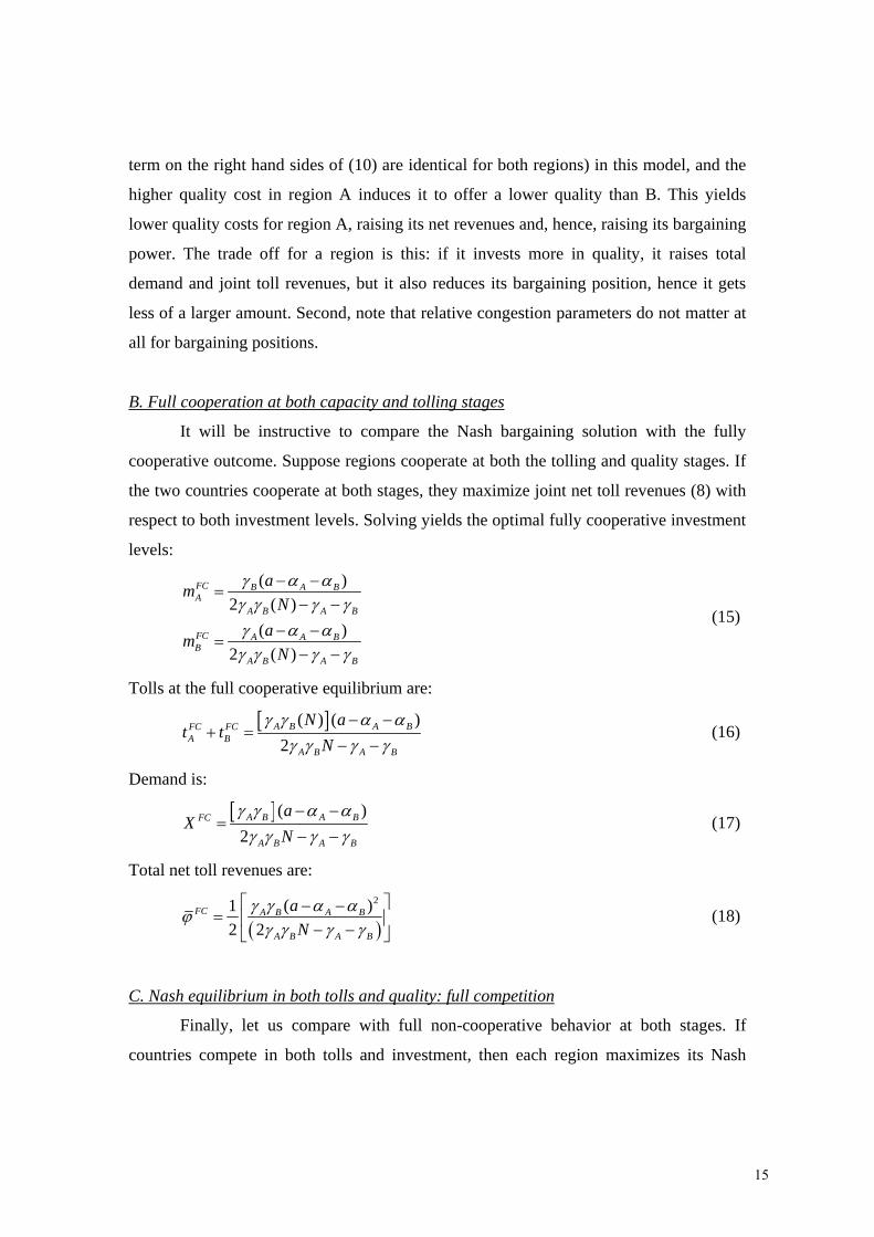
B. Full cooperation at both capacity and tolling stages

It will be instructive to compare the Nash bargaining solution with the fully

cooperative outcome. Suppose regions cooperate at both the tolling and quality stages. If

the two countries cooperate at both stages, they maximize joint net toll revenues (8) with

respect to both investment levels. Solving yields the optimal fully cooperative investment

levels:

( )2 ( )

( )2 ( )

FC B A BA

A B A B

FC A A BB

A B A B

amN

amN

γ α αγ γ γ γγ α αγ γ γ γ

− −=

− −− −

=− −

(15)

Tolls at the full cooperative equilibrium are:

[ ]( ) ( )2

A B A BFC FCA B

A B A B

N at t

Nγ γ α α

γ γ γ γ− −

+ =− −

(16)

Demand is:

[ ]( )2

A B A BFC

A B A B

aX

Nγ γ α αγ γ γ γ

− −=

− − (17)

Total net toll revenues are:

( )2( )1

2 2FC A B A B

A B A B

aN

γ γ α αϕγ γ γ γ

⎡ ⎤− −= ⎢ ⎥− −⎣ ⎦

(18)

C. Nash equilibrium in both tolls and quality: full competition

Finally, let us compare with full non-cooperative behavior at both stages. If

countries compete in both tolls and investment, then each region maximizes its Nash

15

equilibrium profit, obtained for the Nash equilibrium tolls, conditional on quality

investment levels. These were given by (10). Solving for the Nash equilibrium, we find

the following capacities:

2 ( )9 ( ) 2 2

2 ( )9 ( ) 2 2

NE B A BA

A B A B

NE A A BB

A B A B

amNamN

γ α αγ γ γ γγ α α

γ γ γ γ

− −=

− −− −

=− −

(19)

Tolls at the Nash equilibrium are easily derived as:

[ ]3 ( )9 ( ) 2 2

A B A BNE NEA B

A B A B

N at t

Nγ γ α αγ γ γ γ

− −= =

− − (20)

Moreover, demand is found to be:

[ ]3 ( )9 ( ) 2 2

A B A BNE

A B A B

aX

Nγ γ α αγ γ γ γ

− −=

− − (21)

Finally, total net toll revenues are calculated to be:

[ ][ ]

2( )9 ( ) 2 2

A B A BNE

A B A B

aN

γ γ α αϕ

γ γ γ γ− −

=− −

(22)

D. Comparison of regimes

The various expressions for tolls, quality and demand are summarized in Table 1

for the different regimes. Simple algebra then shows that the relations given in Table 2

hold.

Interpretation is straightforward. First, quality investment is highest under full

cooperation, and it is higher under Nash Bargaining than under full competition. The

reason that it is lower under bargaining than under full cooperation is that regions

strategically provide lower quality to strengthen pre-their bargaining position when

negotiating over net toll revenues. Second, the total toll to travel through regions A and B

is highest under full competition. Interestingly, the total toll is lowest under Nash

bargaining. Although full cooperation and bargaining imply the same toll rules,

conditional on quality, investment in quality is higher under full cooperation. Higher

quality implies higher overall tolls, see before. Demand (and hence congestion and

consumer surplus) is highest under full cooperation, despite the fact that regions

16

maximize net revenues. It is lowest under full competition. Finally, total net revenues

under bargaining are higher than under full competition.

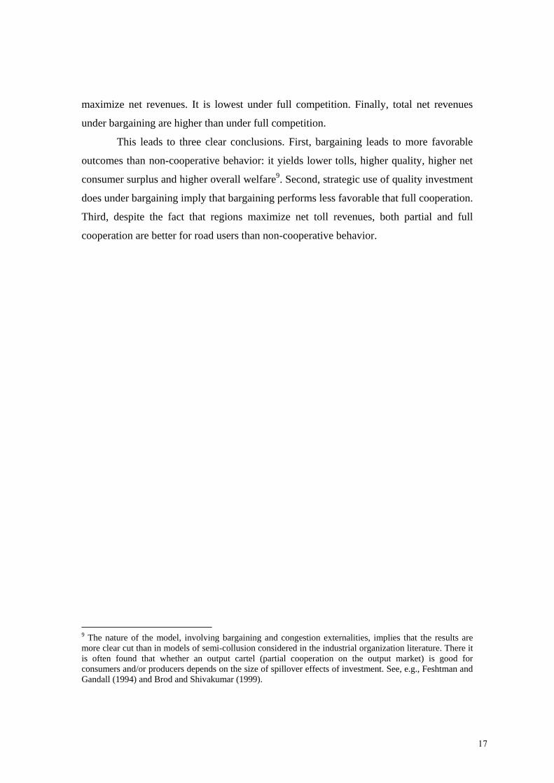
This leads to three clear conclusions. First, bargaining leads to more favorable

outcomes than non-cooperative behavior: it yields lower tolls, higher quality, higher net

consumer surplus and higher overall welfare9. Second, strategic use of quality investment

does under bargaining imply that bargaining performs less favorable that full cooperation.

Third, despite the fact that regions maximize net toll revenues, both partial and full

cooperation are better for road users than non-cooperative behavior.

9 The nature of the model, involving bargaining and congestion externalities, implies that the results are more clear cut than in models of semi-collusion considered in the industrial organization literature. There it is often found that whether an output cartel (partial cooperation on the output market) is good for consumers and/or producers depends on the size of spillover effects of investment. See, e.g., Feshtman and Gandall (1994) and Brod and Shivakumar (1999).

17

Table 1: summary of findings

Nash Bargaining (NB) Full cooperation (FC) Full Nash competition (N

Quality ( )4 ( )

( )4 ( )

NB BA

A B A B

NB AB

A B A B

JmN

JmN

γγ γ γ γ

γγ γ γ γ

=− +

=− +

( )2 ( )

( )2 ( )

FC BA

A B A B

FC AB

A B A B

JmN

JmN

γγ γ γ γ

γγ γ γ γ

=− −

=− −

2 ( )9 ( ) 2 2

2 ( )9 ( ) 2 2

NE BA

A B A

NE AB

A B A

JmN

JmN

γγ γ γ

γγ γ γ

=− −

=− −

Toll levels

2 ( )4 ( )

NB NB A BA B

A B A B

N Jt tNγ γ

γ γ γ γ+ =

− + [ ]( ) ( )

2A BFC FC

A BA B A B

N Jt t

Nγ γγ γ γ γ

+ =− −

[ ]6 (9 ( ) 2

A BNE NEA B

A B

Nt t

Nγ γ

γ γ γ+ =

−

Demand 2 ( )4 ( )

NB A B

A B A B

JXNγ γ

γ γ γ γ=

− + [ ]( )

2A BFC

A B A B

JX

Nγ γ

γ γ γ γ=

− − [ ]3 ( )

9 ( ) 2 2A BNE

A B A

JX

Nγ γ

γ γ γ=

− −

Net revenues [ ]

[ ]

2

2

( ) 8 ( )12 4 ( )

A B A B A B

A B A B

J N

N

γ γ γ γ γ γϕ

γ γ γ γ

⎧ ⎫− +⎪ ⎪= ⎨ ⎬− +⎪ ⎪⎩ ⎭

( )2( )1

2 2FC A B

A B A B

JN

γ γϕγ γ γ γ

⎡ ⎤= ⎢ ⎥− −⎣ ⎦

[ ][

2( )9 ( ) 2 2

A BNE

A B A

JNγ γ

ϕγ γ γ

=− −

Note: ( )A BJ a α α= − −

Table 2: Comparison between regimes

Comparison Nash bargaining (NB), full cooperation (FC) and Full Nash Competition (NE)

Total toll NE>FC>NB

Quality FC>NB>NE

Demand, congestion, consumer surplus

FC>NB>NE

Net revenues FC>NB>NE

18

2.2. Maximizing toll revenues: toll and capacity quality choice under Nash bargaining

In this section, we reconsider the Nash bargaining problem in the case of toll-

capacity decisions, where capacity investment directly reduces congestion at given traffic

levels. Since the methodology is entirely similar to that in the previous section, we

concentrate on the main differences only. Details on the derivation are delegated to

Appendix 1.

Demand is again given by (1). However, following the theoretical transport

literature (see, e.g., Small and Verhoef (2008), De Borger at al. (2007)), we assume the

money plus time cost is a linear function of the volume-capacity ratio. For practical

reasons (see De Palma and Leruth (1989)) it will be instructive to work in terms of

inverse capacity AR . So we specify costs as:

1( , ) ( ),

1( , ) ( ),

A A A A A AA

B B B B B BB

C X R XR RK

C X R XR RK

α β

α β

= + =

= + =

where capacities are denoted ,A BK K . Given these specifications and using user

equilibrium condition (3), we find the reduced-form demand function for traffic as a

function of tolls and capacities:

( , , , ) ,A B A BA B A B A A B B

a t tX t t R R N b R RN

α α β β− − − −= = + + (23)

A. Nash bargaining

At the tolling, stage, regions maximize joint net toll revenues:

[ ],

1 1( ) ( , , , ) ( ) ( )A B

A B A B A B A Bt tA B

Max t t X t t R R k kR R

+ − −

The first order conditions again imply that the joint toll level exceeds marginal external

congestion cost, which is now captured by ( )A A B BR R Xβ β+ . The total tax to pass through

the two countries is shown to be given by:

2

NB NB A BA B

at t α α− −+ = (24)

19

Interestingly, joint toll levels are independent of capacities and the congestion functions’

slope parameters (also see De Borger, Dunkerley and Proost (2008)). Optimal demand is

2

A BaXN

α α− −=

Total toll revenues net of capacity costs equal, after substituting in the objective function: 21 1 1( , ) ( ) ( )

2A B

A B A BA A B B A B

aR R k kb R R R R

α αϕβ β

⎛ ⎞ − −⎡ ⎤= − −⎜ ⎟ ⎢ ⎥+ + ⎣ ⎦⎝ ⎠ (25)

The disagreement Nash equilibrium tolls are easily shown to be:

3

NE NE A BA B

at t α α− −= = (26)

These are higher than the first-best tolls (see (24)). The net revenue levels at the Nash

disagreement levels are, for given capacities:

2

2

1 1( , ) ( )3

1 1( , ) ( )3

NE A BA A B A

A A B B A

NE A BB A B B

A A B B B

aR R kb R R R

aR R kb R R R

α αϕβ β

α αϕβ β

⎛ ⎞ − −⎡ ⎤= −⎜ ⎟ ⎢ ⎥+ + ⎣ ⎦⎝ ⎠

⎛ ⎞ − −⎡ ⎤= −⎜ ⎟ ⎢ ⎥+ + ⎣ ⎦⎝ ⎠

(27)

To see the effect of investing more in capacity on region A’s pre-bargaining

position, it follows from (27) that:

2 0NE NEA B A

A A A

kR R Rϕ ϕ∂ ∂

− = >∂ ∂

.

As before, investing more (in capacity) reduces region A’s pre-bargaining position.

Next, consider the pre-bargaining capacity game. Region A maximizes

{ }* 1( , ) ( , ) ( , ) ( , )2

NE NEA A B A B A A B B A BR R R R R R R Rϕ ϕ ϕ ϕ= + −

with respect to inverse capacity AR . A similar objective function is used by B. The

second-order conditions imply that the capacity reaction functions that follow from the

20

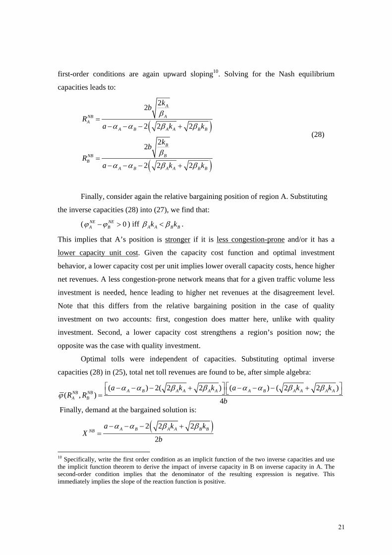
first-order conditions are again upward sloping10. Solving for the Nash equilibrium

capacities leads to:

( )

( )

22

2 2 2

22

2 2 2

A

ANBA

A B A A B B

B

BNBB

A B A A B B

kbR

a k k

kbR

a k k

β

α α β β

β

α α β β

=− − − +

=− − − +

(28)

Finally, consider again the relative bargaining position of region A. Substituting

the inverse capacities (28) into (27), we find that:

( 0NE NEA Bϕ ϕ− > ) iff A A B Bk kβ β< .

This implies that A’s position is stronger if it is less congestion-prone and/or it has a

lower capacity unit cost. Given the capacity cost function and optimal investment

behavior, a lower capacity cost per unit implies lower overall capacity costs, hence higher

net revenues. A less congestion-prone network means that for a given traffic volume less

investment is needed, hence leading to higher net revenues at the disagreement level.

Note that this differs from the relative bargaining position in the case of quality

investment on two accounts: first, congestion does matter here, unlike with quality

investment. Second, a lower capacity cost strengthens a region’s position now; the

opposite was the case with quality investment.

Optimal tolls were independent of capacities. Substituting optimal inverse

capacities (28) in (25), total net toll revenues are found to be, after simple algebra:

( ) 2( 2 2 ) ( ) ( 2 2 )( , )

4A B A A A A A B A A A ANB NB

A B

a k k a k kR R

b

α α β β α α β βϕ

⎡ ⎤ ⎡ ⎤− − − + − − − +⎣ ⎦ ⎣ ⎦=

Finally, demand at the bargained solution is:

( )2 2 2

2A B A A B BNB

a k kX

b

α α β β− − − +=

10 Specifically, write the first order condition as an implicit function of the two inverse capacities and use the implicit function theorem to derive the impact of inverse capacity in B on inverse capacity in A. The second-order condition implies that the denominator of the resulting expression is negative. This immediately implies the slope of the reaction function is positive.

21

B. Comparison of regimes

In Appendix 1 we derive the results under full cooperation and full Nash

competition for this model, using the same procedure as in section 2.1. We summarize

the results obtained for the three regimes considered in Tables 3 and 4. The rankings in

Table 4 are based on the expressions in Table 3 after straightforward, but sometimes

rather extensive, algebra.

Note that the rankings are the same as in the case of quality investment, except for

the toll level. Therefore, bargaining yields more capacity, lower tolls, and both higher net

toll revenues and more consumer benefits for road users than non-cooperative behavior.

22

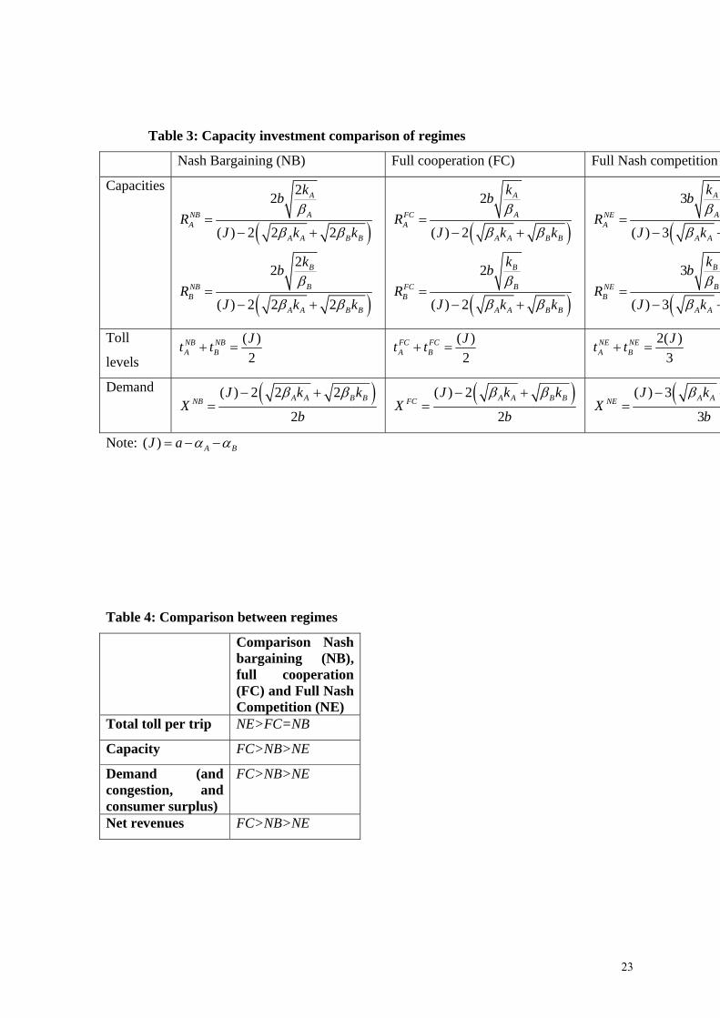
Table 3: Capacity investment comparison of regimes

Nash Bargaining (NB) Full cooperation (FC) Full Nash competition

Capacities

( )

( )

22

( ) 2 2 2

22

( ) 2 2 2

A

ANBA

A A B B

B

BNBB

A A B B

kbR

J k k

kbR

J k k

β

β β

β

β β

=− +

=− +

( )

( )

2

( ) 2

2

( ) 2

A

AFCA

A A B B

B

BFCB

A A B B

kbR

J k k

kbR

J k k

β

β β

β

β β

=− +

=− +

(

(

3

( ) 3

3

( ) 3

A

ANEA

A A

B

BNEB

A A

kbR

J k

kbR

J k

β

β

β

β

=− +

=− +

Toll

levels

( )2

NB NBA B

Jt t+ = ( )2

FC FCA B

Jt t+ = 2( )3

NE NEA B

Jt t+ =

Demand ( )( ) 2 2 2

2A A B BNB

J k kX

b

β β− +=

( )( ) 2

2A A B BFC

J k kX

b

β β− +=

(( ) 3

3A ANE

J kX

b

β− +=

Note: ( ) A BJ a α α= − −

Table 4: Comparison between regimes

Comparison Nash bargaining (NB), full cooperation (FC) and Full Nash Competition (NE)

Total toll per trip NE>FC=NB

Capacity FC>NB>NE

Demand (and congestion, and consumer surplus)

FC>NB>NE

Net revenues FC>NB>NE

23

3. Nash bargaining with a welfare maximizing government

In this section, we extend the model to allow for welfare maximizing

governments. As our purpose is to point out the main differences with revenue

maximizing behavior, we consider the simplest possible setup to illustrate the

implications of taking into account the welfare of road users. Let us, therefore, interpret

the two-region model as in Ubbels and Verhoef (2008). Region A is the city, region B is

the surrounding region. Suppose all traffic in both A and B comes from commuters that

travel from B to A. In such a setting is quite realistic to assume that region B cares about

its commuting inhabitants. As there is no local traffic in the city, region A is assumed not

to care about commuter welfare. So the respective welfare functions that we use are: 2

2

0

0.5 ( )

( ) ( ) 0.5 ( )

A A A AX

X XB B B B

W t X m

W p z dz g X X t X m

γ

γ

= −

⎡ ⎤= − + −⎣ ⎦∫

Here ( ) ( ) ( )XA A A A B B B Bg X X m t X m tα β α β= + + − + + + − is the total generalized cost

(inclusive of toll payments) for a commuting trip. Demand is, as before, given by (4). We

again consecutively consider quality and capacity investment (sections 3.1 and 3.2,

respectively). To avoid too much repetition, we concentrate on the main differences with

the previous section.

3.1. Maximizing welfare: toll and road quality choice under Nash bargaining

A. Nash bargaining

At the tolling stage, regions maximize joint welfare:

,

( , , , ) ( , , , )A B

A A B A B B A B A Bt tMax W t t m m W t t m m+

Using the first-order conditions, it easily follows that the total tax to pass through the two

regions equals the first best marginal external congestion cost:

( )NB NBA B A Bt t Xβ β+ = +

In other words, the toll rule is first-best, conditional on demand. Using (4) we have:

24

[ ]2 2

NB NB A BA B A B A B

A A

t t a m mb

β β α αβ β+

+ = − − + ++ +

(29)

Simple algebra shows that the toll level rises in quality and in the congestion functions’

slope parameters. Note that, for given quality levels, tolls are below those under revenue

maximizing governments (compare with (6)). Optimal demand is

2 2

NB A B A B

A B

a m mXbα α

β β− − + +

=+ +

Total welfare is, after substituting in the objective function: 2

2 2( )( , ) 0.5 0.5 ( ) 0.5 ( )2 2

A B A BA B A A B B

A B

a m mW m m m mbα α γ γ

β β− − + +

= − −+ +

(30)

The disagreement point is the Nash equilibrium in tolls. Country A solves:

[ ] 2( , , , ) 0.5 ( )A

A A B A B A AtMax t X t t m m mγ−

holding quality levels and toll levels in B constant. As before, the first-order conditions

imply that region A charges, conditional on demand, more than marginal external cost:

1 2( )NEAt b Xβ β= + + .

Similarly, region B solves:

2

0

( ) ( ) 0.5 ( )B

XX X

B B Bt

Max p z dz g X X t X mγ⎡ ⎤− + −⎣ ⎦∫

Using the equilibrium condition that generalized price equals generalized cost, we easily

show that the first order condition implies that region B charges exactly the ‘total’

marginal external cost, i.e., it charges for the congestion externality in both regions:

( )NEB A Bt Xβ β= +

The Nash equilibrium tolls are derived as in previous section. We find:

( )

2 3 3

( )2 3 3

NE A BA A B A B

A B

NE A BB A B A B

A B

bt a m mb

t a m mb

β β α αβ β

β β α αβ β

+ += − − + +

+ ++

= − − + ++ +

(31)

Two points are worth noting. First, comparing with (9) we observe that, for given quality

levels, region A charges more and region B charges less than in the case both regions

25

were maximizing toll revenues. Region B charges less because it cares for commuter

welfare; region A charges more in response, given a negatively sloped reaction function.

Second, tolls charged by A exceed those for region B: there is tax exporting by the city

region A (also see De Borger et al. (2007), Ubbels and Verhoef (2008)).

Demand at the disagreement point is given by:

2 3 3

NE A B A B

A B

a m mXb

α αβ β

− − + +=

+ + (32)

Using (31) and (32) in the respective objective functions, the welfare levels at the

Nash disagreement point are shown to be, for given quality levels:

( )( )

2 2

2 2

( , ) ( ) 0.5 ( )

( , ) 0.5 ( ) 0.5 ( )

NE NEA A B A B A A

NE NEB A B A B B B

W m m b X m

W m m b X m

β β γ

β β γ

= + + −

= + + − (33)

For equal quality cost parameters and quality levels, region A has a stronger pre-

bargaining position. The reason is that, for given investment levels, it charges a higher

toll than B and hence has larger revenues. Region B is weaker a priori because it wants a

lower toll than A to account for commuter surplus. Interestingly, therefore, caring for

consumers weakens region B’s pre-bargaining position.

The effect of more quality by region A on its bargaining position is given by:

( )2( )

2 3 3

NE NEA B A B A B

A AA A A B

W W b a m m mm m b

α α γβ β

∂ ∂ − − + +− = −

∂ ∂ + +

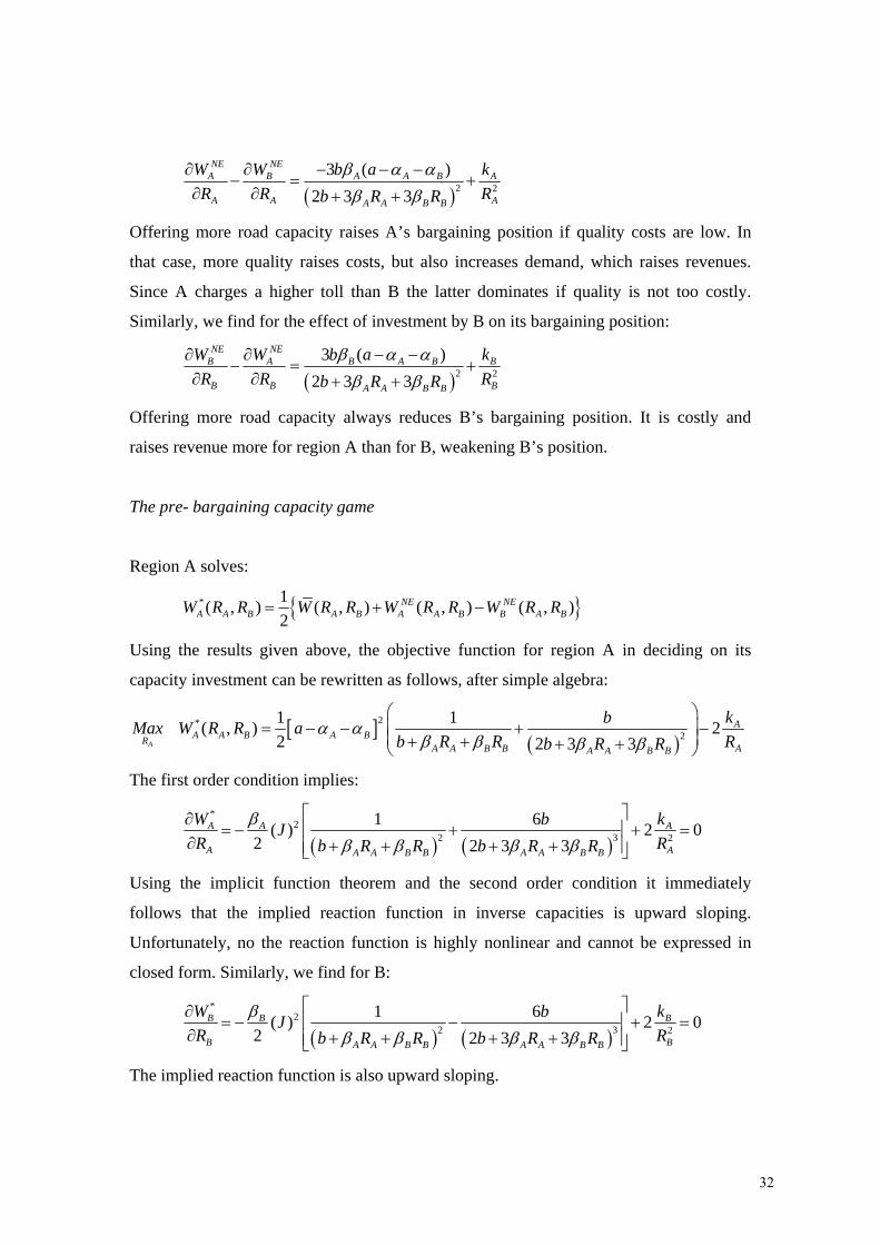
Offering more road quality raises A’s bargaining position if quality costs are low. In that

case, more quality raises costs, but also increases demand, which raises revenues. Since

A charges a higher toll than B the latter dominates if quality is not too costly. Similarly,

we find for the effect of investment by B on its bargaining position:

( )2( )

2 3 3

NE NEB A A B A B

B BB B A B

W W b a m m mm m b

α α γβ β

∂ ∂ − − + +− = − −

∂ ∂ + +

Offering better road quality always reduces B’s bargaining position. It is costly and raises

revenue more for region A than for B, weakening B’s position.

Finally, let us turn to the pre-bargaining quality investment game. Country A

decides on quality by maximizing:

{ }* 1( , ) ( , ) ( , ) ( , )2

NE NEA A B A B A A B B A BW m m W m m W m m W m m= + −

26

The first order condition for region A implies the following reaction function in quality:

( )2( ) 1,

2 2 2 2 2 3 3A B A A

A B AA A A A A B A B

a Z Z bm m ZZ Z b b

α αγ γ β β β β

− −= + = +

− − + + + + (34)

Reaction functions are upward sloping by the second-order conditions. A similar problem

is solved by B. The corresponding reaction function is:

( )2( ) 1,

2 2 2 2 2 3 3A B B B

B A BB B B B A B A B

a Z Z bm m ZZ Z b b

α αγ γ β β β β

− −= + = −

− − + + + + (35)

Solving for the Nash equilibrium capacities yields:

( )2

( )2

NB B A A BA

A B B A A B

NB A B A BB

A B B A A B

Z amZ Z

Z amZ Z

γ α αγ γ γ γγ α αγ γ γ γ

− −=

− −− −

=− −

(36)

Note that, since A BZ Z> it follows that, assuming equal quality investment costs, the city

region, interested in only its toll revenue, will actually invest more: NB NBA Bm m> . The

intuition is clear. If a region invests in more quality this is translated in more demand and

hence higher tolls in both regions, but given the toll rules more so in A than B. The

higher toll, however, reduces consumer surplus for commuters; hence, region B has an

incentive to invest less in quality than A.

The bargaining position of A is captured by NE NEA BW W− , where both are evaluated

at the bargaining quality outcomes. We find, using (36) in (33):

( ) ( )2 2

2 2( ) 40.5 ( ) ( )

2 2 3 3NE NE A B A B A B

A B A B B AA B A B B A A B

aW W Z ZZ Z b

γ γ α α γ γ γ γγ γ γ γ β β

⎡ ⎤ ⎧ ⎫− − ⎪ ⎪− = + −⎢ ⎥ ⎨ ⎬− − + +⎢ ⎥ ⎪ ⎪⎣ ⎦ ⎩ ⎭

Note that this expression is always positive, unless the capacity cost parameter in B is

very large. This makes sense: under ‘normal’ conditions A has a stronger bargaining

position than B, as argued before. However, if the capacity cost in B is very high then B

has a stronger position: it invests much less in quality, leading to lower demand but also

lower tolls. Given the regions’ pricing policies this effect is more important for A than for

B. Moreover, the toll reduction is appreciated by B because it raises consumer surplus of

commuters. Both factors reduce the city region’s relative position.

Toll levels at the Nash bargaining solution are:

27

2 ( )2 2 2

NB NB A B A B A BA B

A A A B B A A A

at tb Z Z

β β γ γ α αβ β γ γ γ γ

⎡ ⎤+ − −+ = ⎢ ⎥+ + − −⎣ ⎦

(37)

Demand is given by

[ ]( )2 ( )

2 2 2NB A B A B

A B B A A B A A

aXZ Z bγ γ α α

γ γ γ γ β β− −

=− − + +

B. Comparison of regimes

In Appendix 2 we work out the analytics of full cooperation and full competition,

and we provide details on the comparison of the results between the three regimes. The

various comparisons of tolls, qualities, welfare levels, etc. are algebraically cumbersome,

but the final results are quite similar to previous findings in Section 2. They are

summarized in Table 5.

The main insight from this section is that bargaining partially resolves problems

typically associated with tax and investment competition. The literature has shown that

(see, e.g., De Borger, Dunkerley and Proost (2007) and Ubbels and Verhoef (2008)) Nash

competition in both tolls and investment implies excessively high tolls and insufficient

investment compared to the first best fully cooperative optimum, implying substantial

welfare losses. We find that partial cooperation through Nash bargaining yields more

investment, lower tolls and higher welfare than fully non-cooperative behavior. However,

as regions use investment to affect their pre-bargaining position, welfare losses compared

to the first-best do remain.

28

Table 5: Comparison between regimes

Comparison Nash bargaining (NB), full cooperation (FC) and Full Nash Competition (NE)

Total toll per trip FC>NB NE>FC, unless demand very elastic and not much congestion

Quality investment FC>NB>NE

Demand (and congestion, and consumer surplus)

FC>NB>NE

Welfare FC>NB>NE

3.2. Maximizing welfare: toll and capacity investment under Nash bargaining

Finally, we considered a model with welfare maximizing regions and investment

in road capacity. As before, generalized cost functions are:

1( ) ( ), ,

1( ) ( ), ,

A A A A A A A AA A

B B B B B B B BB B

XC q q q XR RK KXC q q q XR RK K

α β

α β

= + = = =

= + = = =

We showed in Section 2 that the demand function for traffic is:

( , , , ) ,A B A BA B A B A A B B

a t tX t t R R N b R RN

α α β β− − − −= = + +

The regions welfare functions can now be written as, respectively:

0

( ) ( )

AA A

AX

X X BB B

B

kW t XR

kW p z dz g X X t XR

= −

⎡ ⎤= − + −⎣ ⎦∫

The main difference with earlier analysis is that no closed-form solutions are

available for optimal capacities, neither under bargaining nor under Nash competition.

However, to the extent that analytical results can be derived, they are similar to those in

29

previous sections. This suggests that many of the results of previous sections are likely to

carry over to this case, but that only numerical analysis can provide more information.

We briefly go over the main steps of the analysis.

A. Nash bargaining

Nash bargaining: the tolling stage

Let the regions maximize joint welfare:

,

0

( ) ( )A B

XX X A B

A B A Bt tA B

k kMax W W p z dz g X X t X t XR R

⎡ ⎤+ = − + + − −⎣ ⎦∫

The first order conditions immediately imply the first-best toll regime:

( )A B A A B Bt t R R Xβ β+ = +

This amounts to charging the total marginal external cost of the commuting trip in both

regions.

Using the demand function this can be rewritten as

[ ]( )( 2 2 )

A A B BA B A B

A A B B

R Rt t ab R R

β β α αβ β

++ = − −

+ +

Unlike in case of revenue maximizing governments, the joint toll level now does depend

on capacity provision. One easily shows that more capacity, since it reduces congestion,

leads to lower tolls. Demand is, substituting toll levels:

( )( 2 2 )

NB A B

A A B B

aXb R R

α αβ β− −

=+ +

Total joint welfare equals, after substituting in the objective function: 2( )1( , )

2A B A B

A BA A B B A B

a k kW R Rb R R R R

α αβ β

⎛ ⎞− −= − −⎜ ⎟+ +⎝ ⎠

Nash bargaining: the disagreement point

The disagreement point is the Nash equilibrium in tolls. Country A’s first order condition

implies:

30

( )A A A B Bt bX R R Xβ β= + +

implying that a revenue maximizing city charges more than the overall marginal external

cost. The implied reaction function is easily derived as:

12 2A B

A Bat tα α− −

= −

The first order condition for region B implies:

( )B A A B Bt R R Xβ β= +

The reaction function is:

[ ]( ) ( )( 2 2 ) ( 2 2 )

A A B B A A B BB A B A

A A B B A A B B

R R R Rt a tb R R b R R

β β β βα αβ β β β

+ += − − −

+ + + +

Solving yields the Nash equilibrium tolls

[ ]

[ ]

2 3 3

2 3 3

NE A A B BA A B

A A B B

NE A A B BB A B

A A B B

b R Rt ab R R

R Rt ab R R

β β α αβ β

β β α αβ β

+ += − −

+ ++

= − −+ +

Note that NE NEA Bt t> . Traffic at the Nash equilibrium is:

2 3 3A B

A A B B

aXb R R

α αβ β− −

=+ +

The welfare levels at the Nash disagreement levels are

2

2

( , ) ( )2 3 3

1( , ) ( 2 2 )2 2 3 3

NE A B AA A B A A B B

A A B B A

NE A B BB A B A A B B

A A B B B

a kW R R b R Rb R R R

a kW R R b R Rb R R R

α αβ ββ β

α αβ ββ β

⎡ ⎤− −= + + −⎢ ⎥+ +⎣ ⎦

⎡ ⎤− −= + + −⎢ ⎥+ +⎣ ⎦

Note by simple differentiation that more capacity in region A raises welfare in B (it raises

congestion in B but also toll levels); the same holds in the other direction.

Note that, for equal quality cost parameters and quality levels, region A has again

a stronger pre-bargaining position. The reason is that, for given investment levels, it

charges a higher toll than B and hence has larger revenues. Region B is weaker a priori

because it wants a lower toll than A to account for commuter surplus. The effect of

inverse capacity for region A on its bargaining position is given by:

31

( )2 2

3 ( )2 3 3

NE NEA B A A B A

A A AA A B B

W W b a kR R Rb R R

β α αβ β

∂ ∂ − − −− = +

∂ ∂ + +

Offering more road capacity raises A’s bargaining position if quality costs are low. In

that case, more quality raises costs, but also increases demand, which raises revenues.

Since A charges a higher toll than B the latter dominates if quality is not too costly.

Similarly, we find for the effect of investment by B on its bargaining position:

( )2 2

3 ( )2 3 3

NE NEB A B A B B

B B BA A B B

W W b a kR R Rb R R

β α αβ β

∂ ∂ − −− = +

∂ ∂ + +

Offering more road capacity always reduces B’s bargaining position. It is costly and

raises revenue more for region A than for B, weakening B’s position.

The pre- bargaining capacity game

Region A solves:

{ }* 1( , ) ( , ) ( , ) ( , )2

NE NEA A B A B A A B B A BW R R W R R W R R W R R= + −

Using the results given above, the objective function for region A in deciding on its

capacity investment can be rewritten as follows, after simple algebra:

[ ]( )

2*2

1 1( , ) 22 2 3 3A

AA A B A BR

A A B B AA A B B

kbMax W R R ab R R Rb R R

α αβ β β β

⎛ ⎞= − − + −⎜ ⎟

⎜ ⎟+ + + +⎝ ⎠

The first order condition implies:

( ) ( )

*2

2 3 2

1 6( ) 2 02 2 3 3

A A A

A AA A B B A A B B

W kbJR Rb R R b R R

ββ β β β

⎡ ⎤∂= − + + =⎢ ⎥

∂ + + + +⎢ ⎥⎣ ⎦

Using the implicit function theorem and the second order condition it immediately

follows that the implied reaction function in inverse capacities is upward sloping.

Unfortunately, no the reaction function is highly nonlinear and cannot be expressed in

closed form. Similarly, we find for B:

( ) ( )

*2

2 3 2

1 6( ) 2 02 2 3 3

B B B

B BA A B B A A B B

W kbJR Rb R R b R R

ββ β β β

⎡ ⎤∂= − − + =⎢ ⎥

∂ + + + +⎢ ⎥⎣ ⎦

The implied reaction function is also upward sloping.

32

The set of reaction functions imply, assuming equal investment costs and

congestion levels in both regions, that the city region A offers more capacity, just as in

the case of revenue maximizing governments. Since no explicit solution for inverse

capacities can be derived, the dependency of the relative bargaining strengths on

parameters cannot be derived analytically either.

B. Full cooperation

Full cooperation leads to the following first order conditions:

( )

( )

22 2

22 2

1( ) 02

1( ) 02

A A

A AA A B B

B B

B BA A B B

kW JR Rb R R

kW JR Rb R R

ββ β

ββ β

⎡ ⎤∂= − + =⎢ ⎥

∂ + +⎢ ⎥⎣ ⎦⎡ ⎤∂

= − + =⎢ ⎥∂ + +⎢ ⎥⎣ ⎦

C. Full competition

Nash equilibrium capacities cannot be determines analytically either. For

example, the first order condition for region A can be written as:

( )2

3 2

4 3 3( ) 02 3 3

NEA A A B B A

AA AA A B B

W b R R kJR Rb R R

β βββ β

⎡ ⎤∂ + += − + =⎢ ⎥

∂ + +⎢ ⎥⎣ ⎦

It is highly nonlinear in inverse capacities.

D. Comparison

Although no explicit solutions are available, we can show that the ranking of

capacities is the same as before in Section 2. To show this, assume that the first-order

condition for region A under full cooperation holds, i.e.:

( )

22 2

1( ) 02

A A

A AA A B B

kW JR Rb R R

ββ β

⎡ ⎤∂= − + =⎢ ⎥

∂ + +⎢ ⎥⎣ ⎦

33

Using the first order condition under Nash bargaining this information is shown to imply

that

*

0A

A

WR

∂>

∂

This means that the relations describing the first order conditions for region A under

bargaining and full competition do not intersect, and that the reaction function under

bargaining lies above the condition under full cooperation. A similar exercise for region

B then yields the outcome that the equilibrium capacities under bargaining are below

those under full cooperation, just as in Section 2.

4. A numerical example

We consider a simple numerical example of the tolling and capacity case

considered for welfare maximizing governments. This case (section 3.2) did not yield an

analytical solution. The setting is as in Ubbels and Verhoef (2008). Assume a city (A) is

surrounded by a region (B). Let the distances all users drive be as in the following figure:

<---------10km-----------------><------------------------------20km------------------------------->

A B

4.1 Calibration of the reference situation

Assume current demand is X=500. Given the design of the roads, free flowing

speeds are 50 and 100 kilometer per hour in A and B, respectively. Currently measured

average speeds amount to 20 and 50, respectively. The price elasticity of demand with

respect to the generalized price is assumed to be -0.25. Moreover, capacities in the two

regions are given by 800, 1000A BK K= = , respectively. Current toll levels are zero.

The cost functions to be calibrated are

( )

( )

1,

1,

A A A A AA

B B B B BB

C XR RK

C XR RK

α β

α β

= + =

= + =

34

Assume the monetary cost is 0.1 euro per kilometer, and let time values amount to 10

euro per hour. Then the parameters ,A Bα α reflect the monetary plus time cost at freely

flowing traffic. Given the information above, they can be calibrated as: 3, 4A Bα α= = 11

The money plus time costs at the current traffic flow are easily determined as

follows. First consider region A. Each driver faces the monetary cost of 1 euro, plus a

time cost equal to 5 euro: 10 kilometers at 20km/hour is 0.5 hours, times 10 euro per hour

yields 5 euro. Therefore, we have 3 (500 / 800) 6A AC β= + = . This gives 4.8Aβ = . So we

have 3 4.8( )A AC XR= + . Similarly, a driver in B faces currently a monetary cost of 2 euro

plus a time cost, given average speed of 50 km/hour, of 4 euro. Hence,

4 (500 /1000) 6B BC β= + = or 4Bβ = , and 4 4( )B BC XR= + .

The inverse demand function is

p a bX= −

where p is the generalized price. Given the current generalized costs in A and B equal to

6 and 6, respectively, the reference p=12. Combining with observed demand X=500 and

assuming a price elasticity of -0.25, this allows us to calibrate the demand function as:

15 0.006p X= −

Finally, to calibrate reasonable capacity cost parameters we assumed that the

currently observed equilibrium is the optimal outcome of the Nash competition model at

very low toll levels. The capacity costs obtained were: 0.3, 0.25A Bk k= = .

4.2. Numerical results

In Table 5 we summarize the results of the numerical analysis. We determined

optimal toll and capacity levels under full cooperation (FC), Nash bargaining (NB) and

the fully non-cooperative Nash equilibrium solution (NE).

11 To see this, take A as an example. The cost for traveling the 10 kilometer through A at freely flowing traffic amounts to 1 euro (monetary cost) plus 2 euro (50 kilometer per hour implies 10 kilometer takes 0.2 hours, times 10 euro per hour is 2 euro).

35

Reference Full cooperation (FC)

Nash bargaining (NB)

Full non-cooperative competition (NE)

Toll A+B 0 1.73 2.84 5.07

Toll A 0 2.92

Toll B 0 2.15

Capacity A 800 3866 1289 564

Capacity B 1000 3866 1095 490

Traffic level X 500 758 385 129

Welfare Gain relative to reference for A+B

0 100 95 31

Table 5: numerical results

The results are easily interpreted. First, non-cooperative behavior implies an

enormous increase in toll levels due to tax competition. Cooperation at both the tolling

and capacity stage implies a toll of 1.73 euro in order to capture marginal external

congestion costs, which are unaccounted for in the reference. Second, observe that the

Nash bargaining approach to partial cooperation produces much less extreme results

compared to non-cooperative behavior. It implies a somewhat higher toll compared to

full cooperation, and capacity levels rise only moderately compared to the reference.

Since offering more capacity raises A’s bargaining power, more capacity of offered by A

than B. By investing more regions A secures a larger share of the toll revenues. Third and

most importantly, note that the relative welfare gain of the Nash bargaining solution is

relatively close to the first best outcome of full cooperation: it attains 95% of the welfare

gain the first best attains, relative to the reference case of un-tolled congestion. Non-

cooperative behavior only produces, through charging for congestion, a moderate gain of

some 31% of the maximum attainable gain.

Although the example is extremely simple, what these findings might suggest is

that partial cooperation may in fact lead to welfare results that are far less dramatic than

aggressive competitive behavior. If this is the case, and given that bargaining between

36

governments is the rule rather than the exception, welfare results may be much less

averse than suggested by some recent literature.

5. Concluding comments

We presented a model of partial cooperation between regions or countries in toll

and investment (both quality and capacity investments are considered) setting along a

serial transport corridor, where each link is operated by a different government. To study

partial cooperation, we assumed that countries cooperate at the tolling stage and negotiate

over the distribution of the net benefits knowing that, if no bargaining agreement is

reached, they fall back at the Nash equilibrium of the non-cooperative tolling game. At

the investment stage of the game, countries then strategically compete in order to ensure

a better bargaining position and to get a larger share of the net benefits of the policy

decisions. We compared the results with those of full cooperation and full competition at

both stages of the game.

Findings of this paper include the following. First, in a model of toll and quality

competition, we find that regions’ relative bargaining positions positively depend on the

cost of quality: the region where the cost of quality is higher has the strongest position.

Intuitively, the specification of the investment cost function implies that a higher

marginal quality cost reduces investment spending, increasing (net of capacity costs) toll

revenues. Second, considering a model of toll and capacity decisions we find that a

region’s pre-bargaining position negatively depends on both the slope of the congestion

function and on the unit cost of capacity. Third, partial cooperation implies lower tolls

and higher quality and capacity investment than under the full Nash equilibrium in both

tolls and capacities. Fourth, the region concerned about user welfare weakens its

bargaining position. Finally, partial cooperation (Nash bargaining) yields higher welfare

than full Nash competition. Partial cooperation therefore substantially reduces the welfare

loss associated with fierce toll and capacity competition under full Nash competition, as

pointed out in the recent literature. Of course, since partial cooperation still does not

achieve the first best, some welfare losses do remain.

Extensions to the analysis of this paper include the following. First, although the

idea of partial cooperation is applicable to many other setting as well, a more complete

37

model is needed to guarantee the generality of the results. For example, our model

focused on through traffic only and ignored local transport. Second, more detailed

numerical analysis might provide information on the remaining welfare losses of partial

cooperation. Third, empirical work may be needed to provide evidence on the relevance

of bargained outcomes in tax and capacity competition issues.

38

References

d’Aspremont, C. and A. Jacquemin, Cooperative and Noncooperative R&D in duopoly with spillovers, American Economic Review 78 (5), 1988, 1133-1137. Borck, R. and M. Pflüger, Agglomeration and tax competition, European Economic Review 2006 Brod, A. and R. Shivakumar, Advantageous semi-collusion, The Journal of Industrial Economics XLVII (2), 1999, 221-230. De Borger, B., Dunkerley, F. and S. Proost, Strategic investment and pricing decisions in a congested transport corridor, Journal of Urban Economics 62 (2), 2007, 294-316. De Borger, B., Dunkerley, F. and S. Proost, The interaction between tolls and capacity investment in parallel and serial transport networks, Review of Network Economics 7, 2008, 136-158. De Borger, B., Proost, S. and K. Van Dender, Congestion and tax competition on a parallel network, European Economic Review 49 (8), 2005, 2013-2040. de Palma, A. and L. Leruth, Congestion and game in capacity: a duopoly analysis in the presence of network externalities, Annales d’Economie et de Statistique 15/16, 1989, 389-407. Fershtman, C. and E. Muller, Capital investments and price agreements in semi-collusive markets, Rand Journal of Economics 17 (2), 1986, 214-226. Han, S. and J. Leach, A bargaining model of tax competition, Journal of Public

Economics 92, 2008, 1122-1141. Janeba, E., Tax competition when governments lack commitment, American Economic

Review 2000 Kanbur, A. and M. Keen, Jeux sans frontières: tax competition when countries differ in size, American Economic Review 83, 1993, 877-892. Keen, M. and C. Kotsiogannis, Leviathan and capital tax competition in federations, Journal of Public Economic Theory, 2003 Levinson, D., Why States Toll – An empirical model of finance choice, Journal of Transport Economics and Policy 35 (2), 2001, 223-238 Mintz, J. and H. Tulkens, Commodity taxation between member states of a federation: equilibrium and efficiency, Journal of Public Economics 29, 1986, 173-197.

39

Nash, J.F., The bargaining problem, Econometrica 18, 1950, 155-162. Parry, I., How large are the welfare costs of tax competition?, Journal of Urban Economics 54, 2003, 39-60. Pauwels, W. and P. Kort, R&D investments in semicollusive markets with bargaining between asymmetric firms, Working paper, Department of Economics, University of Antwerp, 2008 Salvanes, K.G., Steen, F. and L. Sorgard, Collude, compete or both, Journal of Transport Economics and Policy 37 (3), 2003, 383-416. Sorensen, P., Tax coordination: its desirability and redistributional implications, Economic Policy 15, 2000, 431-472. Ubbels, B. and E. Verhoef, Governmental competition in road charging and capacity choice, Regional Science and Urban Economics, 2008 Wilson, J.S., Theories of tax competition, National Tax Journal LII, 1999, 269-304. Wilson, J.D. and D. Wildasin, Capital tax competition: bane or boon, Journal of Public Economics 2004 Zodrow, G.R., Tax competition and tax coordination in the European Union, International Tax and Public Finance 2003

40

Appendix 1: the case of capacity investment for revenue maximizing regions.

In this appendix, we provide details on the cases of full cooperation and full Nash

competition.

Full cooperation at both capacity and tolling stages

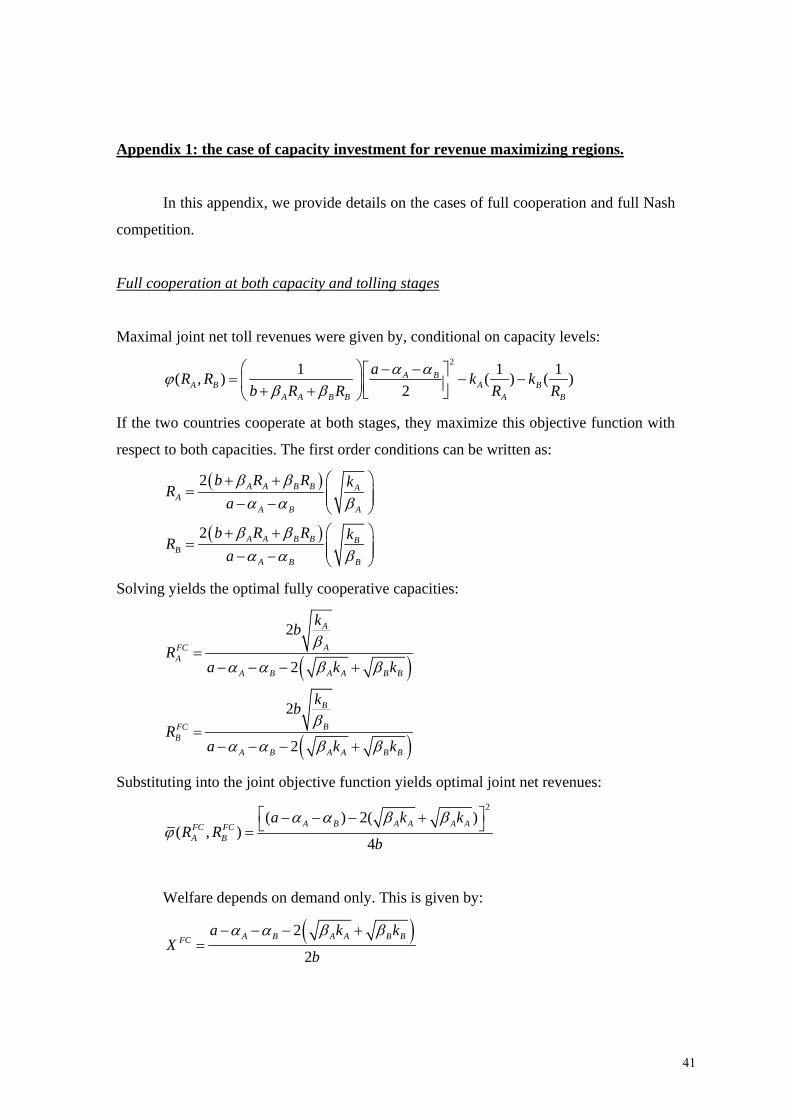
Maximal joint net toll revenues were given by, conditional on capacity levels:

21 1 1( , ) ( ) ( )

2A B

A B A BA A B B A B

aR R k kb R R R R

α αϕβ β

⎛ ⎞ − −⎡ ⎤= − −⎜ ⎟ ⎢ ⎥+ + ⎣ ⎦⎝ ⎠

If the two countries cooperate at both stages, they maximize this objective function with

respect to both capacities. The first order conditions can be written as:

( )

( )

2

2

A A B B AA

A B A

A A B B BB

A B B

b R R kRa

b R R kRa

β βα α β

β βα α β

⎛ ⎞+ += ⎜ ⎟⎜ ⎟− − ⎝ ⎠

⎛ ⎞+ += ⎜ ⎟⎜ ⎟− − ⎝ ⎠

Solving yields the optimal fully cooperative capacities:

( )

( )

2

2

2

2

A

AFCA

A B A A B B

B

BFCB

A B A A B B

kbR

a k k

kbR

a k k

β

α α β β

β

α α β β

=− − − +

=− − − +

Substituting into the joint objective function yields optimal joint net revenues: 2

( ) 2( )( , )

4A B A A A AFC FC

A B

a k kR R

b

α α β βϕ

⎡ ⎤− − − +⎣ ⎦=

Welfare depends on demand only. This is given by:

( )2

2A B A A B BFC

a k kX

b

α α β β− − − +=

41

Nash equilibrium in both tolls and capacities: full competition

If countries compete in both tolls and capacities, then they maximize the Nash

equilibrium profit, obtained for the Nash equilibrium tolls, conditional on capacities.

These were given by, for A and B respectively: 2

2

1 1( , ) ( )3

1 1( , ) ( )3

NE A BA A B A

A A B B A

NE A BB A B B

A A B B B

aR R kb R R R

aR R kb R R R

α αϕβ β

α αϕβ β

⎛ ⎞ − −⎡ ⎤= −⎜ ⎟ ⎢ ⎥+ + ⎣ ⎦⎝ ⎠

⎛ ⎞ − −⎡ ⎤= −⎜ ⎟ ⎢ ⎥+ + ⎣ ⎦⎝ ⎠

This leads to the Nash equilibrium capacities:

( )

( )

3

3

3

3

A

ANEA

A B A A B B

B

BNEB

A B A A B B

kbR

a k k

kbR

a k k

β

α α β β

β

α α β β

=− − − +

=− − − +

The regions’ net revenues are, respectively:

( ) 3( ) ( ) 33 3

( ) 3( ) ( ) 33 3

A B A A B B A B A ANEA

A B A A B B A B B BNEB

a k k a kb

a k k a kb

α α β β α α βϕ

α α β β α α βϕ

⎡ ⎤ ⎡ ⎤− − − + − − −= ⎢ ⎥ ⎢ ⎥⎢ ⎥ ⎢ ⎥⎣ ⎦ ⎣ ⎦⎡ ⎤ ⎡ ⎤− − − + − − −

= ⎢ ⎥ ⎢ ⎥⎢ ⎥ ⎢ ⎥⎣ ⎦ ⎣ ⎦

They get less if they have higher capacity costs or congestion. Total net toll revenues

under this regime are: 2

( ) 3( )13

A B A A B BNE NE NEA B

a k kb

α α β βϕ ϕ ϕ

⎡ ⎤− − − +⎛ ⎞= + = ⎢ ⎥⎜ ⎟⎝ ⎠ ⎢ ⎥⎣ ⎦

Demand is given by:

( )3

3A B A A B BNE

a k kX

b

α α β β− − − +=

42

Appendix 2. Comparison between regimes: welfare maximizing governments

In this appendix we work out the other regimes (full cooperation and full

competition) and compare with the results for Nash bargaining.

First, consider full cooperation. Maximal joint welfare with respect to both quality

levels yields the optimal fully cooperative levels:

( )( 2 2 ) ( )

( )( 2 2 ) ( )

FC B A BA

A B A B A B

FC A A BB

A B A B A B

amb

amb

γ α αγ γ β β γ γ

γ α αγ γ β β γ γ

− −=

+ + − +− −

=+ + − +

Tolls at the full cooperative equilibrium are:

( ) ( )( 2 2 ) ( )

FC FC A B A BA B A B

A B A B A B

at tbγ γ α αβ β

γ γ β β γ γ− −

+ = ++ + − +

Demand is given by

( )( 2 2 ) ( )

FC A B A B

A B A B A B

aXbγ γ α α

γ γ β β γ γ− −

=+ + − +

Second, if countries compete in both tolls and qualities, then they maximize the

Nash equilibrium welfare, conditional on qualities. The relevant expressions were given

in the main body of the paper, for A and B respectively. Working out the first order

conditions for region A, its reaction function can be written as:

( )2( ) 2( ),

2 3 3A B A A A B

A B AA A A A A B

a Q Q bm m QQ Q b

α α β βγ γ β β

− − + += + =

− − + + (A1)

Similarly, we find for B:

( )2( ) 2 2,

2 3 3A B B B A B

B B BB B B B A B

a Q Q bm m QQ Q b

α α β βγ γ β β

− − + += + =

− − + + (A2)

This leads to the Nash equilibrium qualities:

( ) ( );NE NEB A A B A B A BA B

A B A B B A A B A B B A

Q a Q am mQ Q Q Q

γ α α γ α αγ γ γ γ γ γ γ γ

− − − −= =

− − − −

This implies the city region offers more quality than the regional authority. Substituting

in the Nash demand function we have:

43

[ ][ ]( )

2 3 3NE A B A B

A B A B B A A B

aXQ Q bγ γ α α

γ γ γ γ β β− −

=− − + +

Finally, the toll per trip is:

[ ][ ] [ ]

2 2 ( )2 3 3

A BNE NE A B A BA B

A B A B A B B A

b at tb Q Q

β β γ γ α αβ β γ γ γ γ

+ + − −+ =

+ + − −

Comparing the results under the three regimes, let us start with investment in

quality. It is straightforward to show that bargaining implies lower quality than full

cooperation. To compare bargaining with full competition, the key point to note is that

both the intercept and the slopes of the reaction functions of the capacity game under

bargaining and Nash competition can be directly compared. For example, the relative

intercepts and slopes of the reaction functions for A depend on the comparison of

2

A

A A

ZZγ −

and A

A A

QQγ −

Using the relevant definitions (see (34) and (A1)) it immediately follows that Nash

competition implies both a lower intercept and lower slope that bargaining. A similar

reasoning holds for the reaction functions for B. Since the reaction functions are linear,

this implies that

FC NB NEA A Am m m> >

FC NB NEB B Bm m m> >

Next consider demand under the different regimes. We find again that FC NB NEX X X> >

To see this, direct comparison yields, after some simple algebra, that

FC NBX X>

where the difference is smallest when we have B Aγ γ> and this difference is large. In that

case B has large bargaining power and can obtain better outcomes for commuter welfare.

Toll rules are the same under these regimes, but more overall quality is offered under

cooperation. This implies also that from the consumer’s viewpoint cooperation is always

better than bargained outcomes, but that the difference is smallest when region B has

44

substantial bargaining power; this happens when its marginal quality cost is much larger

than for than for A.

To show that demand will be higher under bargaining than full competition, use

(4) to write:

1 ( )NB NE NB NB NE NE NB NB NE NEA B A B A B A BX X m m m m t t t t

N⎡ ⎤− = + − − − + − −⎣ ⎦

Substituting the toll rules:

( )

( 2 2 )

NB NB NBA B A BNE NE NEA B A B

t t X

t t b X

β β

β β

+ = +

+ = + +

into this expression and working out, we have:

1 ( )2 2

NB NE NB NB NE NE NBA B A B A B

A B

X X m m m m b Xb

β ββ β

⎡ ⎤− = + − − + + +⎣ ⎦+ +

This is necessarily positive, since more quality is offered under bargaining than

competition.

Next, let us compare toll levels. Note that the toll rules are the same under full

cooperation and bargaining, but more overall quality is offered under cooperation. So the

toll per trip is higher under full cooperation than under bargaining: FC FC NB NBA B A Bt t t t+ > +

One expects the toll per trip under competition to be higher than the first-best toll, given

that competition, conditional on demand, implies a toll which largely exceeds marginal

external congestion cost. However, it also yields lower demand. To appreciate this start

from the rules:

( )

( 2 2 )

FC FC FCA B A BNE NE NEA B A B

t t X

t t b X

β β

β β

+ = +

+ = + +

For given demand, tolls are much higher under full competition than bargaining, but

demand is lower (see above), reducing tolls. The toll difference can be written as:

( ) ( ) ( )( ) ( )FC FC NE NE FC NE NEA B A B A B A Bt t t t X X b Xβ β β β+ − + = + − − + +

The first term on the right hand side is positive, the second negative. Surprisingly, we

were unable to show in general that the competitive toll exceeds the first best toll. The

same holds for the comparison with bargaining tolls. Clearly, if there is no congestion,

the expression is negative and tolls are higher under competition. The same holds if

45

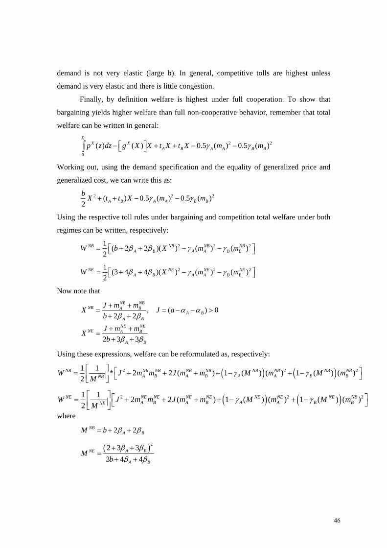
demand is not very elastic (large b). In general, competitive tolls are highest unless

demand is very elastic and there is little congestion.

Finally, by definition welfare is highest under full cooperation. To show that

bargaining yields higher welfare than full non-cooperative behavior, remember that total

welfare can be written in general:

2 2

0

( ) ( ) 0.5 ( ) 0.5 ( )X

X XA B A A B Bp z dz g X X t X t X m mγ γ⎡ ⎤− + + − −⎣ ⎦∫

Working out, using the demand specification and the equality of generalized price and

generalized cost, we can write this as:

2 2 2( ) 0.5 ( ) 0.5 ( )2 A B A A B Bb X t t X m mγ γ+ + − −

Using the respective toll rules under bargaining and competition total welfare under both

regimes can be written, respectively:

2 2 21 ( 2 2 )( ) ( ) ( )2

NB NB NB NBA B A A B BW b X m mβ β γ γ⎡ ⎤= + + − −⎣ ⎦

2 2 21 (3 4 4 )( ) ( ) ( )2

NE NE NE NEA B A A B BW X m mβ β γ γ⎡ ⎤= + + − −⎣ ⎦

Now note that

, ( ) 0

2 2

2 3 3

NB NBNB A B

A BA B

NE NENE A B

A B

J m mX J ab

J m mXb

α αβ β

β β

+ += = − − >

+ +

+ +=

+ +

Using these expressions, welfare can be reformulated as, respectively:

( ) ( )2 2 21 1 * 2 2 ( ) 1 ( ) ( ) 1 ( ) ( )2

NB NB NB NB NB NB NB NB NBA B A B A A B BNBW J m m J m m M m M m

Mγ γ⎡ ⎤ ⎡ ⎤= + + + + − + −⎢ ⎥ ⎣ ⎦⎣ ⎦

( ) ( )2 2 21 1 2 2 ( ) 1 ( ) ( ) 1 ( ) ( )2

NE NE NE NE NE NE NE NE NBA B A B A A B BNEW J m m J m m M m M m

Mγ γ⎡ ⎤ ⎡ ⎤= + + + + − + −⎢ ⎥ ⎣ ⎦⎣ ⎦

where

2 2NBA BM b β β= + +

( )22 3 33 4 4

A BNE

A B

Mb

β ββ β

+ +=

+ +

46

Using ,NB NE NB NEA A B Bm m m m> > , and noting that NB NEM M< it immediately follows that

welfare under bargaining is higher than under full competition.

47

Documents de Treball de l’IEB

2007 2007/1. Durán Cabré, J.Mª.; Esteller Moré, A.: "An empirical analysis of wealth taxation: Equity vs. tax compliance" 2007/2. Jofre-Monseny, J.; Solé-Ollé, A.: "Tax differentials and agglomeration economies in intraregional firm location" 2007/3. Duch, N.; Montolio, D.; Mediavilla, M.: "Evaluating the impact of public subsidies on a firm’s performance: A quasi experimental approach" 2007/4. Sánchez Hugalde, A.: "Influencia de la inmigración en la elección escolar" 2007/5. Solé-Ollé, A.; Viladecans-Marsal, E.: "Economic and political determinants of urban expansion: Exploring the local connection" 2007/6. Segarra-Blasco, A.; García-Quevedo, J.; Teruel-Carrizosa, M.: "Barriers to innovation and public policy in Catalonia" 2007/7. Calero, J.; Escardíbul, J.O.: "Evaluación de servicios educativos: El rendimiento en los centros públicos y privados medido en PISA-2003" 2007/8. Argilés, J.M.; Duch Brown, N.: "A comparison of the economic and environmental performances of conventional and organic farming: Evidence from financial statement" 2008 2008/1. Castells, P.; Trillas, F.: "Political parties and the economy: Macro convergence, micro partisanship?" 2008/2. Solé-Ollé, A.; Sorribas-Navarro, P.: "Does partisan alignment affect the electoral reward of intergovernmental transfers?" 2008/3. Schelker, M.; Eichenberger, R.: "Rethinking public auditing institutions: Empirical evidence from Swiss municipalities" 2008/4. Jofre-Monseny, J.; Solé-Ollé, A.: "Which communities should be afraid of mobility? The effects of agglomeration economies on the sensitivity of firm location to local taxes" 2008/5. Duch-Brown, N.; García-Quevedo, J.; Montolio, D.: "Assessing the assignation of public subsidies: do the experts choose the most efficient R&D projects?" 2008/6. Solé-Ollé, A.; Hortas Rico, M.: "Does urban sprawl increase the costs of providing local public services? Evidence from Spanish municipalities" 2008/7. Sanromà, E.; Ramos, R.; Simón, H.: "Portabilidad del capital humano y asimilación de los inmigrantes. Evidencia para España" 2008/8. Trillas, F.: "Regulatory federalism in network industries" 2009 2009/1. Rork, J.C.; Wagner, G.A.: "Reciprocity and competition: is there a connection?" 2009/2. Mork, E.; Sjögren, A.; Svaleryd, H.: "Cheaper child care, more children" 2009/3. Rodden, J.: "Federalism and inter-regional redistribution" 2009/4. Ruggeri, G.C.: "Regional fiscal flows: measurement tools" 2009/5. Wrede, M.: "Agglomeration, tax competition, and fiscal equalization" 2009/6. Jametti, M.; von Ungern-Sternberg, T.: "Risk selection in natural disaster insurance" 2009/7. Solé-Ollé, A; Sorribas-Navarro, P.: "The dynamic adjustment of local government budgets: does Spain behave differently?" 2009/8. Sanromá, E.; Ramos, R.; Simón, H.: "Immigration wages in the Spanish Labour Market: Does the origin of human capital matter?" 2009/9. Mohnen, P.; Lokshin, B.: "What does it take for and R&D incentive policy to be effective?" 2009/10. Solé-Ollé, A.; Salinas, P..: "Evaluating the effects of decentralization on educational outcomes in Spain?" 2009/11. Libman, A.; Feld, L.P.: "Strategic Tax Collection and Fiscal Decentralization: The case of Russia" 2009/12. Falck, O.; Fritsch, M.; Heblich, S.: "Bohemians, human capital, and regional economic growth" 2009/13. Barrio-Castro, T.; García-Quevedo, J.: "The determinants of university patenting: do incentives matter?" 2009/14. Schmidheiny, K.; Brülhart, M.: "On the equivalence of location choice models: conditional logit, nested logit and poisson" 2009/15. Itaya, J., Okamuraz, M., Yamaguchix, C.: "Partial tax coordination in a repeated game setting" 2009/16. Ens, P.: "Tax competition and equalization: the impact of voluntary cooperation on the efficiency goal" 2009/17. Geys, B., Revelli, F.: "Decentralization, competition and the local tax mix: evidence from Flanders" 2009/18. Konrad, K., Kovenock, D.: "Competition for fdi with vintage investment and agglomeration advantages" 2009/19. Loretz, S., Moorey, P.: "Corporate tax competition between firms"

Documents de Treball de l’IEB

2009/20. Akai, N., Sato, M.: "Soft budgets and local borrowing regulation in a dynamic decentralized leadership model with saving and free mobility" 2009/21. Buzzacchi, L., Turati, G.: "Collective risks in local administrations: can a private insurer be better than a public mutual fund?" 2009/22. Jarkko, H.: "Voluntary pension savings: the effects of the finnish tax reform on savers’ behaviour" 2009/23. Fehr, H.; Kindermann, F.: "Pension funding and individual accounts in economies with life-cyclers and myopes" 2009/24. Esteller-Moré, A.; Rizzo, L.: "(Uncontrolled) Aggregate shocks or vertical tax interdependence? Evidence from gasoline and cigarettes" 2009/25. Goodspeed, T.; Haughwout, A.: "On the optimal design of disaster insurance in a federation" 2009/26. Porto, E.; Revelli, F.: "Central command, local hazard and the race to the top" 2009/27. Piolatto, A.: "Plurality versus proportional electoral rule: study of voters’ representativeness" 2009/28. Roeder, K.: "Optimal taxes and pensions in a society with myopic agents" 2009/29, Porcelli, F.: "Effects of fiscal decentralisation and electoral accountability on government efficiency evidence from the Italian health care sector" 2009/30, Troumpounis, O.: "Suggesting an alternative electoral proportional system. Blank votes count" 2009/31, Mejer, M., Pottelsberghe de la Potterie, B.: "Economic incongruities in the European patent system" 2009/32, Solé-Ollé, A.: "Inter-regional redistribution through infrastructure investment: tactical or programmatic?" 2009/33, Joanis, M.: "Sharing the blame? Local electoral accountability and centralized school finance in California" 2009/34, Parcero, O.J.: "Optimal country’s policy towards multinationals when local regions can choose between firm-specific and non-firm-specific policies" 2009/35, Cordero, J,M.; Pedraja, F.; Salinas, J.: "Efficiency measurement in the Spanish cadastral units through DEA" 2009/36, Fiva, J.; Natvik, G.J.: "Do re-election probabilities influence public investment?" 2009/37, Haupt, A.; Krieger, T.: "The role of mobility in tax and subsidy competition" 2009/38, Viladecans-Marsal, E; Arauzo-Carod, J.M.: "Can a knowledge-based cluster be created? The case of the Barcelona 22@district"

Fiscal Federalism