NTRODUCTION

Wireless communications, nowadays, depend on antenna as an essential component.

Without the antenna, it would be virtually impossible to have any form of wireless

communication. Instead, the communications would be achieved by cumbersomely

connecting wires between every transmitter and receiver. The world would be

proliferated by an abundance of wires, and the range of available communications

would be very limited to say the least.

The history of the antenna is a relatively young one. Started in 1842, when Joseph

Henry used vertical wires on the roof of his house to detect lightning flashes. Later on,

in 1864, James Clerk Maxwell presented the equations that form the basis for antenna

technology and microwave engineering. In 1885, Thomas Edison patented a

communications system that utilized top-loaded, vertical antennas for telegraphy. Two

years later, Heinrich Hertz introduced a Hertzian dipole to experimentally validate

Maxwell’s equation in regard that electromagnetic waves propagate through the air.

Guglielmo Marconi, in 1898, developed radio commercially and pioneering

transcontinental communications [1].

In 19th century, antennas have been used for lot of applications. The need for radar

during the major wars of the 20th century sparked the creation of large reflectors,

lenses, dipole and waveguide slot arrays. The antenna has been an essential component

of the television set since the 1930’s. The proliferation of antennas in today’s world is

also quite evident. Satellites in orbital space relay information about the weather, in

addition to news of important social and political events around the globe. Radar, an

application of antennas, allows air traffic controllers to track and safely guide aircraft to

their destinations around the world. More recently, antennas serve as vital components

on pagers and cellular phones, devices central to a wireless revolution. Also large radio

astronomy antennas are constantly searching the sky looking for other forms of

intelligent life in the universe. This sampling of antenna topologies and applications is

by no means inclusive; it serves to demonstrate the wide variety and uses of antennas in

practical life.

In this regard, the antenna serves as a link to our past and the key to our future,

measurements of near or far fields from antennas are very expensive and mostly are

1

performed on isolated environments without the effect of the surrounding

structures. Study of the actual antennas interaction with the actual structures is,

computationally and experimentally tedious. The advent of computer technology has

greatly advanced many aspects of amateur radio. In technical areas such as antenna

design, circuit design, and radio propagation, where one depends on empirical

estimations for the experimental methods. Computer software can often help optimize

results much more reliably. The purpose of modeling is to do the design cheaply on the

computer before “bending metal.” The old “cut and try” method works, but it is costly

in time and money (two things perpetually in short supply). If the computer simulation

is used, then time and money would be saved.

Research of this thesis is motivated to use different types of electromagnetic

simulators (EM) such as PCAAD, EZNEC, MATLAB, and MMANA in order to design

different types of dipole antennas and compare the results with the theoretical part and

then analyze each type. Different types of dipole antennas such as Half Wave Dipole

Antenna, Rabbit Ears (V) antenna and Yagi-Uda are going to be constructed and

simulated.

This thesis will prove that modeling and simulation processes makes it possible to

look at more alternatives and to gauge the effect of a change in an antenna design before

the change is made. By using these powerful software, different directivities, gains,

front-to-back ratios, side lobes, input impedances, the patterns of the current,

polarization, radiation in polar and three dimensions can be calculated and displayed in

order to be compared with the theoretical part.

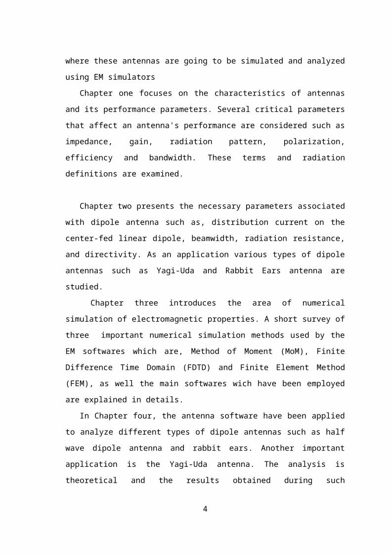
This thesis is organized in four chapters. The first three chapters introduce background

information on antenna parameters, the theory of dipole antennas, modeling methods

and software that are used for antenna simulations. The last chapter focuses on some

applications to linear dipole antenna such as rabbit ears antenna and Yagi-Uda antenna,

where these antennas are going to be simulated and analyzed using EM simulators

Chapter one focuses on the characteristics of antennas and its performance

parameters. Several critical parameters that affect an antenna's performance are

considered such as impedance, gain, radiation pattern, polarization, efficiency and

bandwidth. These terms and radiation definitions are examined.

2

Chapter two presents the necessary parameters associated with dipole antenna such

as, distribution current on the center-fed linear dipole, beamwidth, radiation resistance,

and directivity. As an application various types of dipole antennas such as Yagi-Uda

and Rabbit Ears antenna are studied.

Chapter three introduces the area of numerical simulation of electromagnetic

properties. A short survey of three important numerical simulation methods used by the

EM softwares which are, Method of Moment (MoM), Finite Difference Time Domain

(FDTD) and Finite Element Method (FEM), as well the main softwares wich have been

employed are explained in details.

In Chapter four, the antenna software have been applied to analyze different types

of dipole antennas such as half wave dipole antenna and rabbit ears. Another important

application is the Yagi-Uda antenna. The analysis is theoretical and the results obtained

during such simulations will be explained in details using Tables and Figures.

An implementation design will be also introduced for Yagi-Uda antenna which is to

be simulated in accordance with broadcasting channels of Bayrak Radyo ve Televizyon

Kurumu (BRTK) in Turkish Republic of Northern Cyprus (TRNC). Finally, conclusions

are given and the possible future extension to this model will be mentioned.

3

CHAPTER ONE

ANTENNA PARAMETERS

1.1 Overview

Antenna is a metallic structure designed for radiating and receiving electromagnetic

energy. It acts as a transitional structure between the guiding device (e.g. waveguide,

transmission line) and the free space. There are several critical parameters that affect

an antennas performance and can be adjusted during the design process. These are

impedance, gain, aperture or radiation pattern, polarization, efficiency and bandwidth.

In this chapter the principles and characteristics of antennas and its performance

parameters are examined.

1.2 Electromagnetic Radiation

Electromagnetic radiation includes radio waves, microwaves, infrared radiation, visible

light, ultraviolet waves, X-rays, and gamma rays. Together they make up the

electromagnetic spectrum. They all move at the speed of light . The only

difference between them is their wavelength (the distance a wave travels during

one complete cycle [vibration]), which is also directly related to the amount of energy

the waves carry.

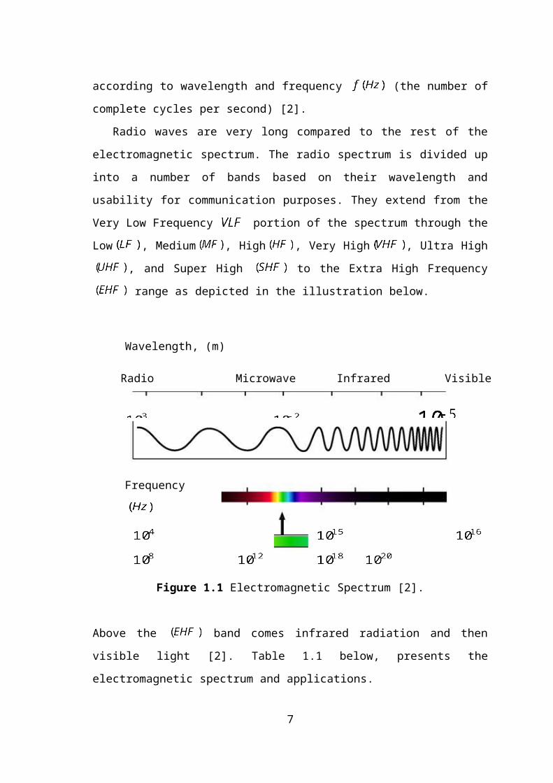
The shorter the wavelength, the higher the energy. Figure 1.1 lists the

electromagnetic spectrum components according to wavelength and frequency

(the number of complete cycles per second) [2].

Radio waves are very long compared to the rest of the electromagnetic spectrum.

The radio spectrum is divided up into a number of bands based on their wavelength and

usability for communication purposes. They extend from the Very Low Frequency

portion of the spectrum through the Low , Medium , High , Very High

, Ultra High , and Super High to the Extra High Frequency

range as depicted in the illustration below.

4

Figure 1.1 Electromagnetic Spectrum [2].

Above the band comes infrared radiation and then visible light [2]. Table 1.1

below, presents the electromagnetic spectrum and applications.

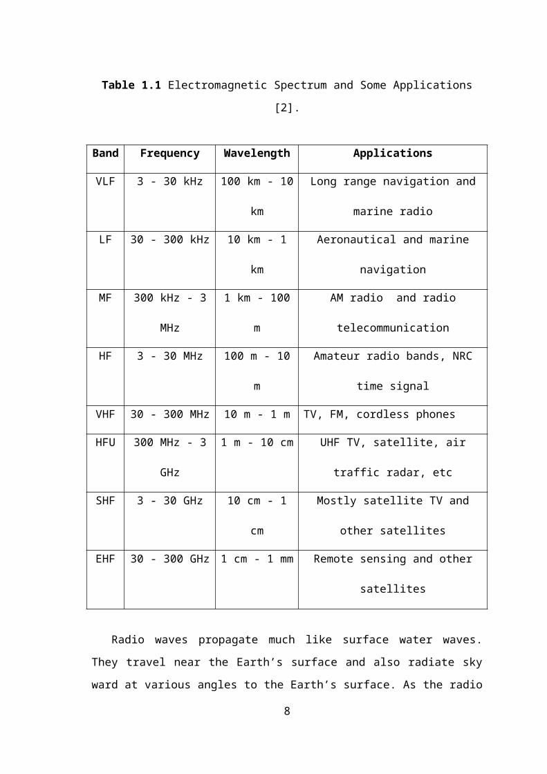
Table 1.1 Electromagnetic Spectrum and Some Applications [2].

Band Frequency Wavelength Applications

VLF 3 - 30 kHz 100 km - 10 km Long range navigation and marine radio

LF 30 - 300 kHz 10 km - 1 km Aeronautical and marine navigation

MF 300 kHz - 3 MHz 1 km - 100 m AM radio and radio telecommunication

HF 3 - 30 MHz 100 m - 10 m Amateur radio bands, NRC time signal

VHF 30 - 300 MHz 10 m - 1 m TV, FM, cordless phones

HFU 300 MHz - 3 GHz 1 m - 10 cm UHF TV, satellite, air traffic radar, etc

SHF 3 - 30 GHz 10 cm - 1 cm Mostly satellite TV and other satellites

EHF 30 - 300 GHz 1 cm - 1 mm Remote sensing and other satellites

5

Wavelength, (m)

Radio Microwave Infrared Visible Ultraviolet X-Ray Gamma Ray

Frequency

Radio waves propagate much like surface water waves. They travel near the Earth’s

surface and also radiate sky ward at various angles to the Earth’s surface. As the radio

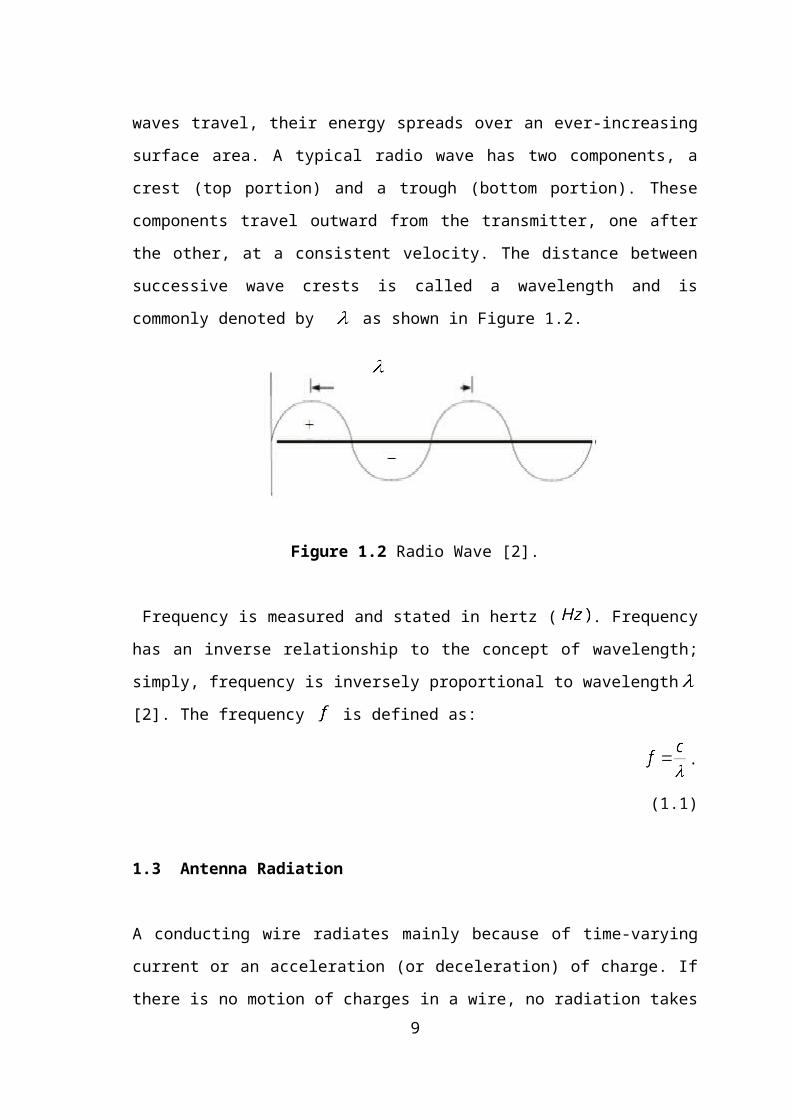
waves travel, their energy spreads over an ever-increasing surface area. A typical radio

wave has two components, a crest (top portion) and a trough (bottom portion). These

components travel outward from the transmitter, one after the other, at a consistent

velocity. The distance between successive wave crests is called a wavelength and is

commonly denoted by as shown in Figure 1.2.

Figure 1.2 Radio Wave [2].

Frequency is measured and stated in hertz ( . Frequency has an inverse relationship

to the concept of wavelength; simply, frequency is inversely proportional to wavelength

[2]. The frequency is defined as:

. (1.1)

1.3 Antenna Radiation

A conducting wire radiates mainly because of time-varying current or an acceleration

(or deceleration) of charge. If there is no motion of charges in a wire, no radiation takes

place, since no flow of current occurs. Radiation will not occur even if charges are

moving with uniform velocity along a straight wire. However, charges moving with

uniform velocity along a curved or bent wire will produce radiation. If the charge is

oscillating with time, then radiation occurs even along a straight wire [3].

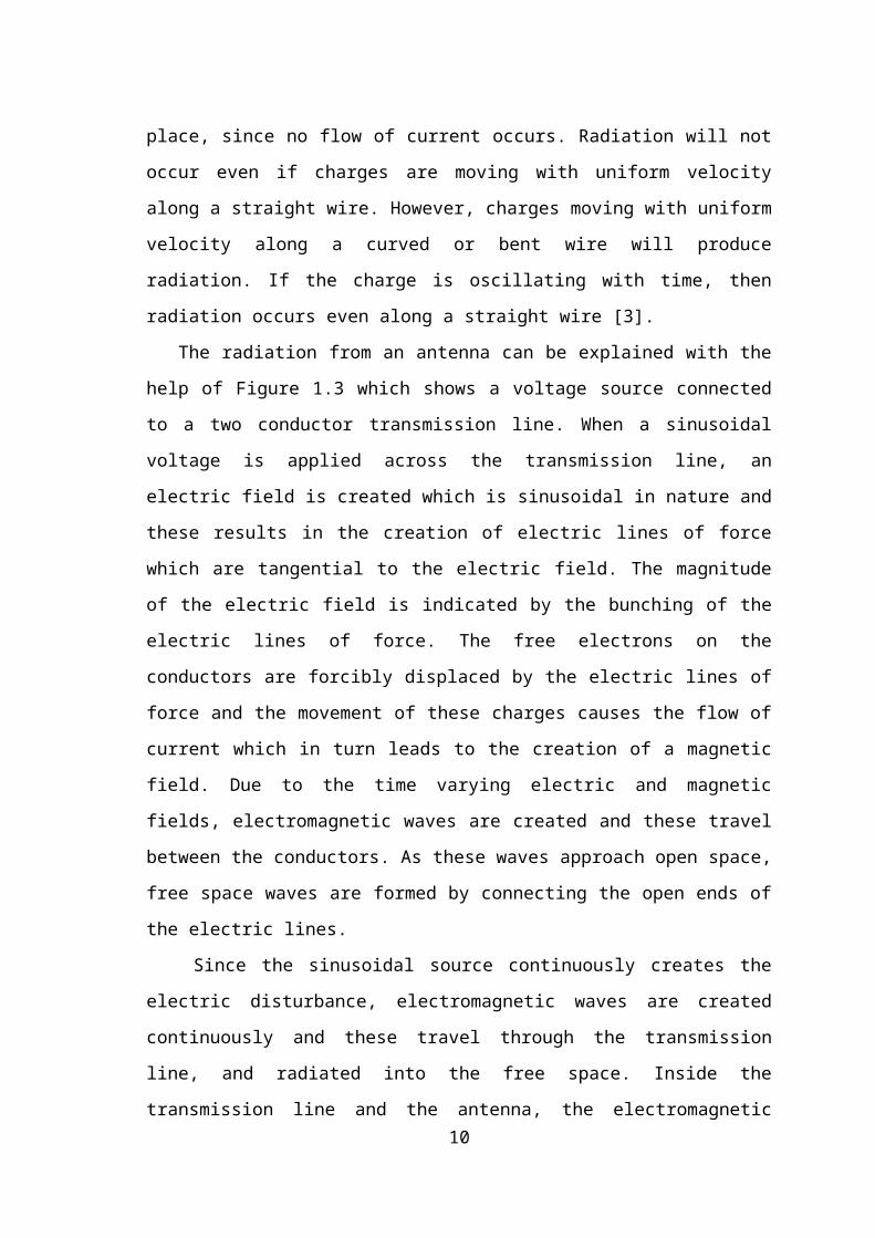
The radiation from an antenna can be explained with the help of Figure 1.3 which

shows a voltage source connected to a two conductor transmission line. When a

sinusoidal voltage is applied across the transmission line, an electric field is created

6

which is sinusoidal in nature and these results in the creation of electric lines of force

which are tangential to the electric field. The magnitude of the electric field is indicated

by the bunching of the electric lines of force. The free electrons on the conductors are

forcibly displaced by the electric lines of force and the movement of these charges

causes the flow of current which in turn leads to the creation of a magnetic field. Due to

the time varying electric and magnetic fields, electromagnetic waves are created and

these travel between the conductors. As these waves approach open space, free space

waves are formed by connecting the open ends of the electric lines.

Since the sinusoidal source continuously creates the electric disturbance,

electromagnetic waves are created continuously and these travel through the

transmission line, and radiated into the free space. Inside the transmission line and the

antenna, the electromagnetic waves are sustained due to the charges, but as soon as they

enter the free space, they form closed loops and are radiated [3].

Figure 1.3 Radiations From an Antenna [3].

7

Transmission line Source Free Space WaveAntenna

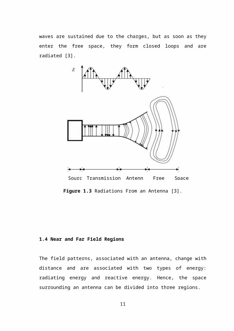
1.4 Near and Far Field Regions

The field patterns, associated with an antenna, change with distance and are associated

with two types of energy: radiating energy and reactive energy. Hence, the space

surrounding an antenna can be divided into three regions.

Figure 1.4 Field Regions Around an Antenna [3].

The three regions shown in Figure 1.4 are:

• Reactive near-field region: In this region, the reactive field dominates. The reactive

energy oscillates towards and away from the antenna, thus appearing as reactance. In

this region, energy is only stored and no energy is dissipated. The outermost boundary

for this region is at a distance

,

(1.2)

where is the distance from the antenna surface, D is the largest dimension of the

antenna and λ is the wavelength. Radiating near-field region (Fresnel region). It is the

region which lies between the reactive near-field region and the far field region.

8

Reactive Near

Field Region

Reactive Near

Field Region

Far Field Region

Radiation Near Field

Region

Reactive fields are smaller in this field as compared to the reactive near-field region and

the radiation fields dominate. In this region, the angular field distribution is a function

of the distance from the antenna. The outermost boundary for this region is at a distance

, (1.3)

where is the distance from the antenna surface.

• Far-field region (Fraunhofer region): The region beyond is the far field

region.

In this region, the reactive fields are absent and only the radiation fields exist. The

angular field distribution is not dependent on the distance from the antenna in this

region and the power density varies as the inverse square of the radial distance in this

region [3].

1.5 Antenna Parameters

The performance of an antenna can be gauged from a number of parameters. Certain

critical parameters are briefly discussed below.

1.5.1 Radiation Pattern

The radiation pattern of an antenna is a plot of the far-field radiation properties of an

antenna as a function of the spatial coordinates which are specified by the elevation

angle and the azimuth angle .

More specifically, it is a plot of the power radiated from an antenna per unit solid

angle which is nothing but the radiation intensity [3]. Let us consider the case of an

isotropic antenna. An isotropic antenna is one which radiates equally in all directions.

If the total power radiated by the isotropic antenna is P, then the power is spread

over a sphere of radius r, so that the power density S at this distance in any direction is

given by

(Watts /m2), (1.4)

and the radiation intensity for this isotropic antenna can be written as

9

(Watts).

(1.5)

An isotropic antenna is not possible to realize in practice and is used only for

comparison purposes. A more practical type is the directional antenna which radiates

more power in some directions and less power in other directions. A special case of the

directional antenna is the omnidirectional antenna whose radiation pattern may be

constant in one plane (e.g., -plane) and varies in an orthogonal plane (e.g., -plane).

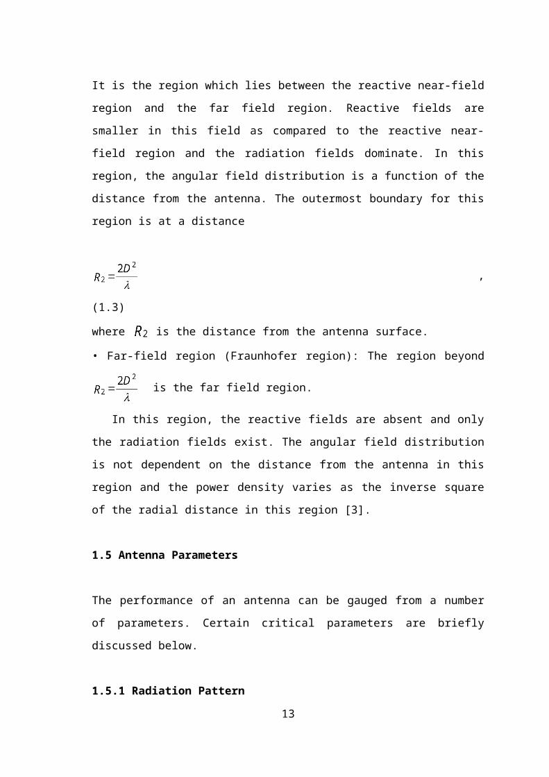
The radiation pattern plot of a generic directional antenna is shown in Figure 1.5.

Figure 1.5 Radiation Pattern of a Directional Antenna [3].

Figure 1.5, the half power beam width (HPBW) can be defined as the angle

subtended by the half power points of the main lobe, main lobe is the radiation lobe

containing the direction of maximum radiation, and minor lobe is all the lobes other

than the main lobe. These lobes represent the radiation in undesired directions. The

level of minor lobes is usually expressed as a ratio of the power density in the lobe in

question to that of the major lobe.

This ratio is called as the side lobe level (expressed in decibels). Back lobe is the

minor lobe diametrically opposite the main lobe; side lobes are the minor lobes adjacent

to the main lobe and are separated by various nulls. Side lobes are generally the largest

among the minor lobes. In most wireless systems, minor lobes are undesired. Hence a

good antenna design should minimize the minor lobes [3].10

Minor Lobes

Back Lobe

Null Side Lobe

Main Lobe

HPBW

1.5.2 Polarization

Polarization of a radiated wave is defined as the property of an electromagnetic wave

describing the time varying direction and relative magnitude of the electric field vector

[3]. The polarization of an antenna refers to the polarization of the electric field vector

of the radiated wave. In other words, the position and direction of the electric field with

reference to the earth’s surface or ground determines the wave polarization.

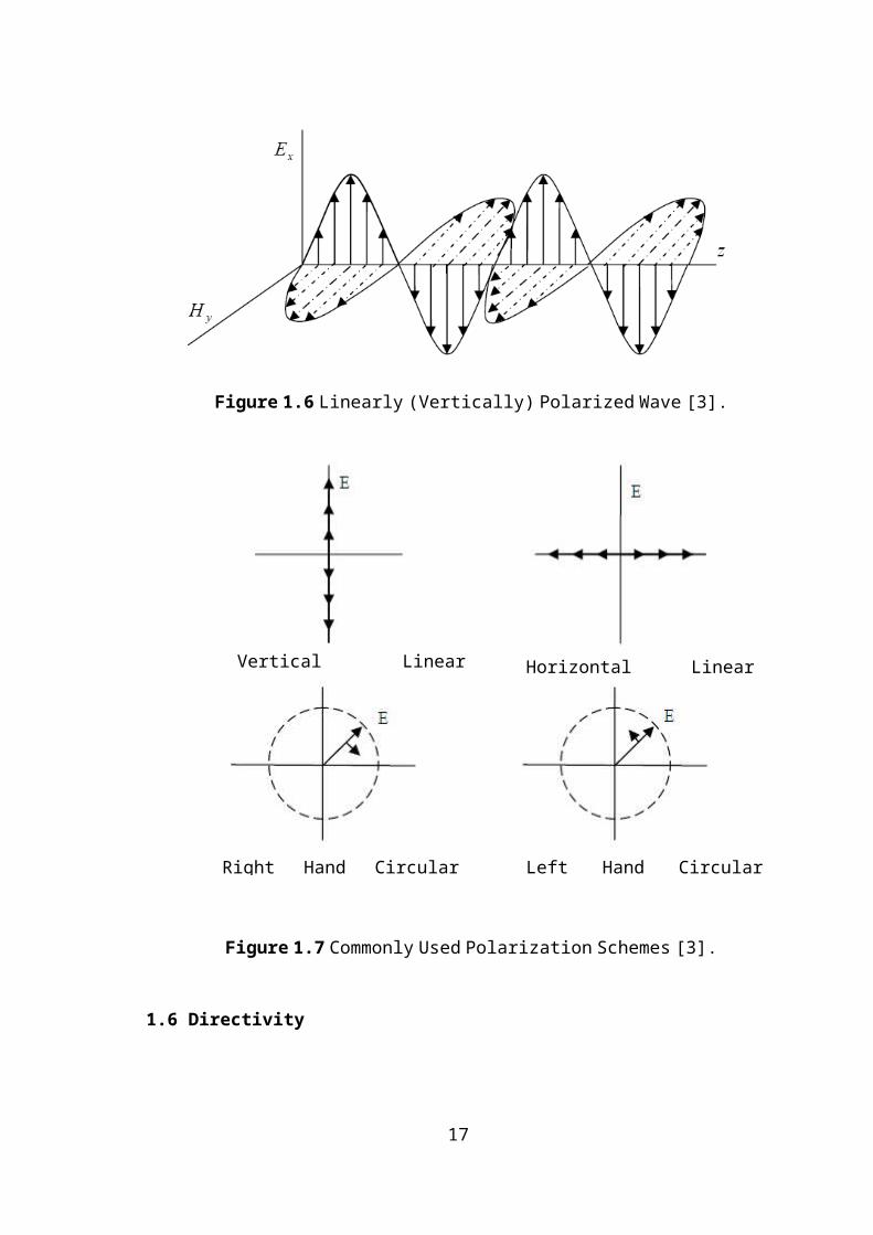
The most common types of polarization include the linear (horizontal or vertical)

and circular (right hand polarization or the left hand polarization). If the path of the

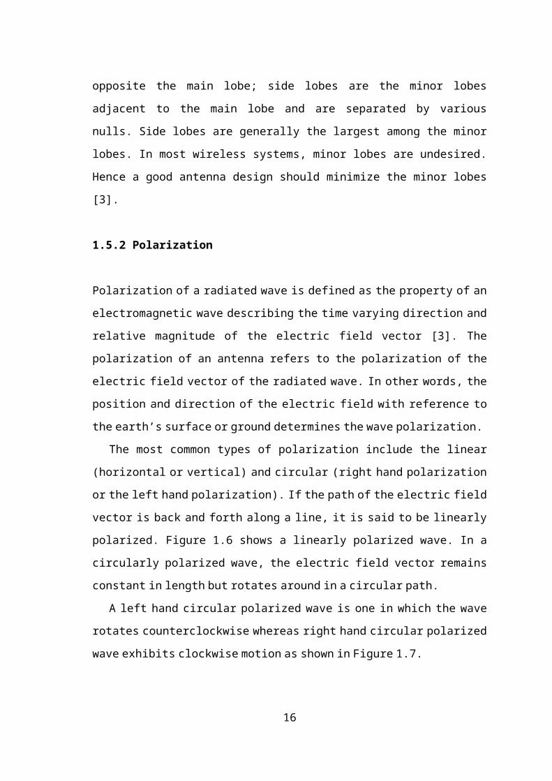
electric field vector is back and forth along a line, it is said to be linearly polarized.

Figure 1.6 shows a linearly polarized wave. In a circularly polarized wave, the electric

field vector remains constant in length but rotates around in a circular path.

A left hand circular polarized wave is one in which the wave rotates

counterclockwise whereas right hand circular polarized wave exhibits clockwise motion

as shown in Figure 1.7.

Figure 1.6 Linearly (Vertically) Polarized Wave [3].

11

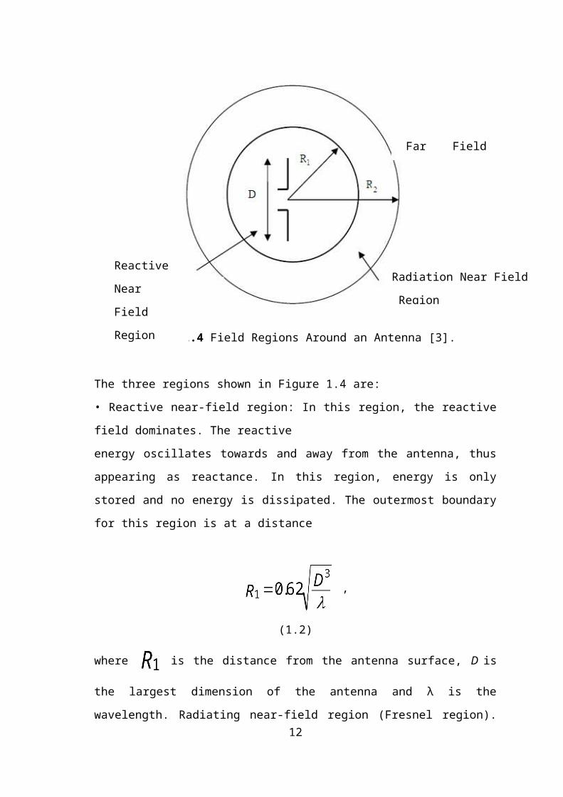
Figure 1.7 Commonly Used Polarization Schemes [3].

1.6 Directivity

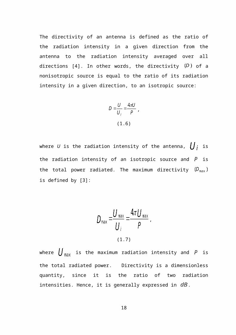
The directivity of an antenna is defined as the ratio of the radiation intensity in a given

direction from the antenna to the radiation intensity averaged over all directions [4]. In

other words, the directivity of a nonisotropic source is equal to the ratio of its

radiation intensity in a given direction, to an isotropic source:

, (1.6)

where U is the radiation intensity of the antenna, is the radiation intensity of an

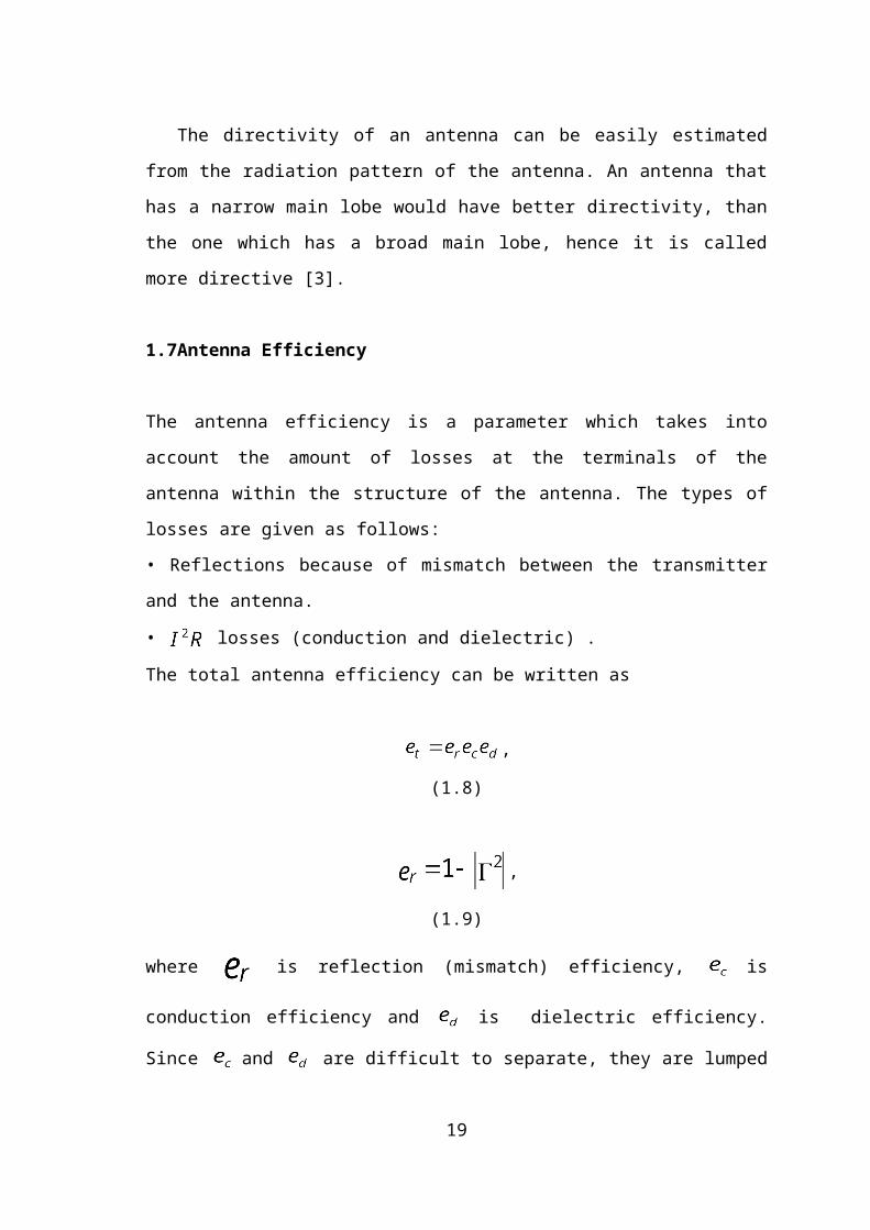
isotropic source and is the total power radiated. The maximum directivity is

defined by [3]:

12

Vertical Linear Polarization Horizontal Linear Polarization

Right Hand Circular Polarization Left Hand Circular Polarization

,

(1.7)

where is the maximum radiation intensity and is the total radiated power.

Directivity is a dimensionless quantity, since it is the ratio of two radiation intensities.

Hence, it is generally expressed in .

The directivity of an antenna can be easily estimated from the radiation pattern of

the antenna. An antenna that has a narrow main lobe would have better directivity, than

the one which has a broad main lobe, hence it is called more directive [3].

1.7Antenna Efficiency

The antenna efficiency is a parameter which takes into account the amount of losses at

the terminals of the antenna within the structure of the antenna. The types of losses are

given as follows:

• Reflections because of mismatch between the transmitter and the antenna.

• losses (conduction and dielectric) .

The total antenna efficiency can be written as

, (1.8)

,

(1.9)

where is reflection (mismatch) efficiency, is conduction efficiency and is

dielectric efficiency. Since and are difficult to separate, they are lumped together

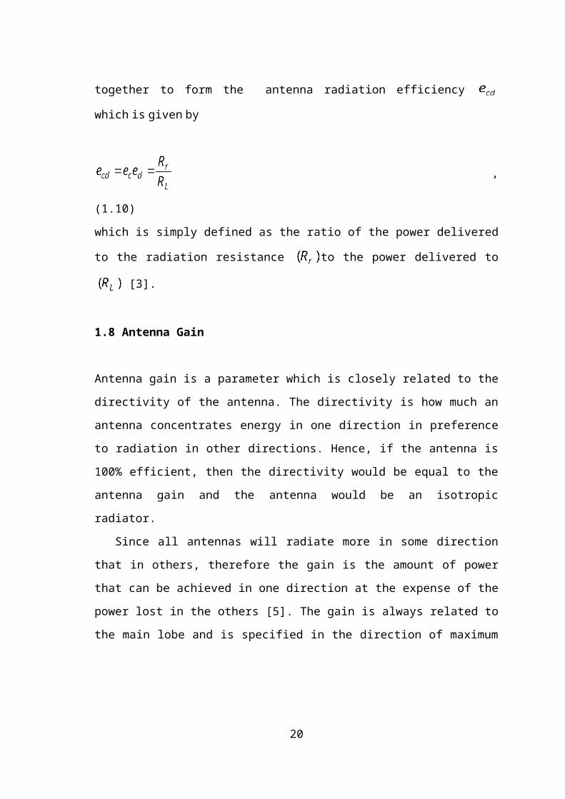
to form the antenna radiation efficiency which is given by

, (1.10)

which is simply defined as the ratio of the power delivered to the radiation resistance

to the power delivered to [3].

1.8 Antenna Gain13

Antenna gain is a parameter which is closely related to the directivity of the antenna.

The directivity is how much an antenna concentrates energy in one direction in

preference to radiation in other directions. Hence, if the antenna is 100% efficient, then

the directivity would be equal to the antenna gain and the antenna would be an isotropic

radiator.

Since all antennas will radiate more in some direction that in others, therefore the

gain is the amount of power that can be achieved in one direction at the expense of the

power lost in the others [5]. The gain is always related to the main lobe and is specified

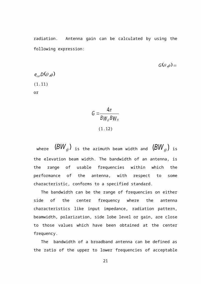
in the direction of maximum radiation. Antenna gain can be calculated by using the

following expression:

(1.11)

or

(1.12)

where is the azimuth beam width and is the elevation beam

width. The bandwidth of an antenna, is the range of usable frequencies within which the

performance of the antenna, with respect to some characteristic, conforms to a specified

standard.

The bandwidth can be the range of frequencies on either side of the center

frequency where the antenna characteristics like input impedance, radiation pattern,

beamwidth, polarization, side lobe level or gain, are close to those values which have

been obtained at the center frequency.

The bandwidth of a broadband antenna can be defined as the ratio of the upper to

lower frequencies of acceptable operation. The bandwidth of a narrowband antenna can

be defined as the percentage of the frequency difference over the center frequency [3].

14

1.9 Front-to-Back Ratio

It is often useful to compare the front-to-back ratio of directional antennas. This is the

ratio of the maximum directivity of an antenna to its directivity in the opposite

direction. For example, when the radiation pattern is plotted on a relative dB scale, the

front-to-back ratio is the difference in dB between the level of the maximum radiation in

the forward direction and the level of radiation at . This number is meaningless for

an omnidirectional antenna, but it gives one an idea of the amount of power directed

forward on a very directional antenna. Front to back can be described by [6].

1.10 Input Impedance

The input impedance of an antenna is defined, as the impedance presented by an

antenna at its terminals or the ratio of the voltage to the current at the pair of terminals

or the ratio of the appropriate components of the electric to magnetic fields at a point

[3]. Hence, the impedance at the teminals of antenna is defined by:

,

(1.13)

where is the antenna resistance and is the antenna reactance. Futher, the

imaginary part , represents the power stored in the near field of the antenna.

Reactance is the imaginary part of electrical impedance, a measure of opposition to a

sinusoidal alternating current. Reactance arises from the presence of inductance and

capacitance within a circuit [7].

The resistive part , consists of two components, the radiation resistance

and the loss resistance . The power associated with the radiation resistance is

the power actually radiated by the antenna, while the power dissipated in the loss

resistance is lost as heat in the antenna itself due to dielectric or conducting losses [3].

1.11 Summary

15

This chapter discussed the definitions and related terminologies regarding antenna,

which are very useful for future studies. The antenna parameters which are associated

with the radiation pattern, the radiation efficiency, the input impedance, and bandwidth

have been discussed. Furthermore, the gain, beam width, polarization, minor lobe level

and radiation efficiency have also been defined.

CHAPTER TWO

THE THEORY OF DIPOLE ANTENNAS AND YAGI UDA

ANTENNA

2.1 Overview

Wire antennas are the most familiar antennas because they are seen virtually

everywhere. There are various shapes of wire antennas such as a straight wire (dipole),

loop and helix antenna. Dipole antennas have been widely used since the early days of

radio communication.

A dipole antenna, developed by Heinrich Rudolph Hertz around 1886 [8], is an

antenna with a center-fed driven element for transmitting or receiving radio frequency

energy. These antennas are the simplest practical antennas from a theoretical point of

view.

This chapter presents the necessary parameters associated with dipole antenna such

as, distribution current on the center-fed linear dipole, beam width, radiation resistance,

and directivity. We further introduce various types of dipole antennas and Yagi-Uda

antenna.

2.2 Thin Linear Dipole Antenna

16

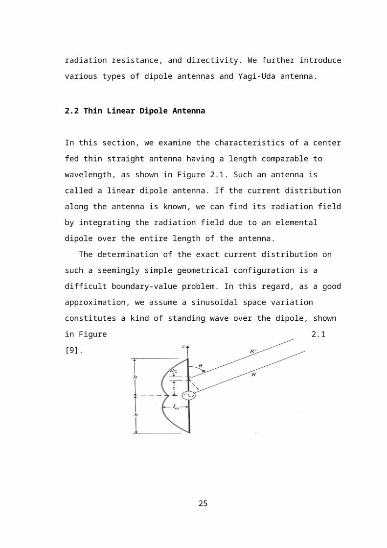
In this section, we examine the characteristics of a center fed thin straight antenna

having a length comparable to wavelength, as shown in Figure 2.1. Such an antenna is

called a linear dipole antenna. If the current distribution along the antenna is known, we

can find its radiation field by integrating the radiation field due to an elemental dipole

over the entire length of the antenna.

The determination of the exact current distribution on such a seemingly simple

geometrical configuration is a difficult boundary-value problem. In this regard, as a

good approximation, we assume a sinusoidal space variation constitutes a kind of

standing wave over the

dipole, shown in Figure

2.1 [9].

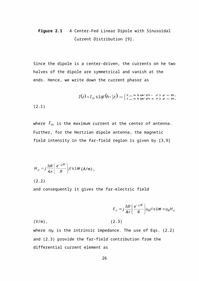
Figure 2.1 A Center-Fed Linear Dipole with Sinusoidal Current Distribution [9].

Since the dipole is a center-driven, the currents on he two halves of the dipole are

symmetrical and vanish at the ends. Hence, we write down the current phasor as

(2.1)

where is the maximum current at the center of antenna. Further, for the Hertzian

dipole antenna, the magnetic field intensity in the far-field region is given by [3,9]

(A/m), (2.2)

and consequently it gives the far-electric field

17

(V/m), (2.3)

where is the intrinsic impedance. The use of Eqs. (2.2) and (2.3) provide the far-field

contribution from the differential current element as

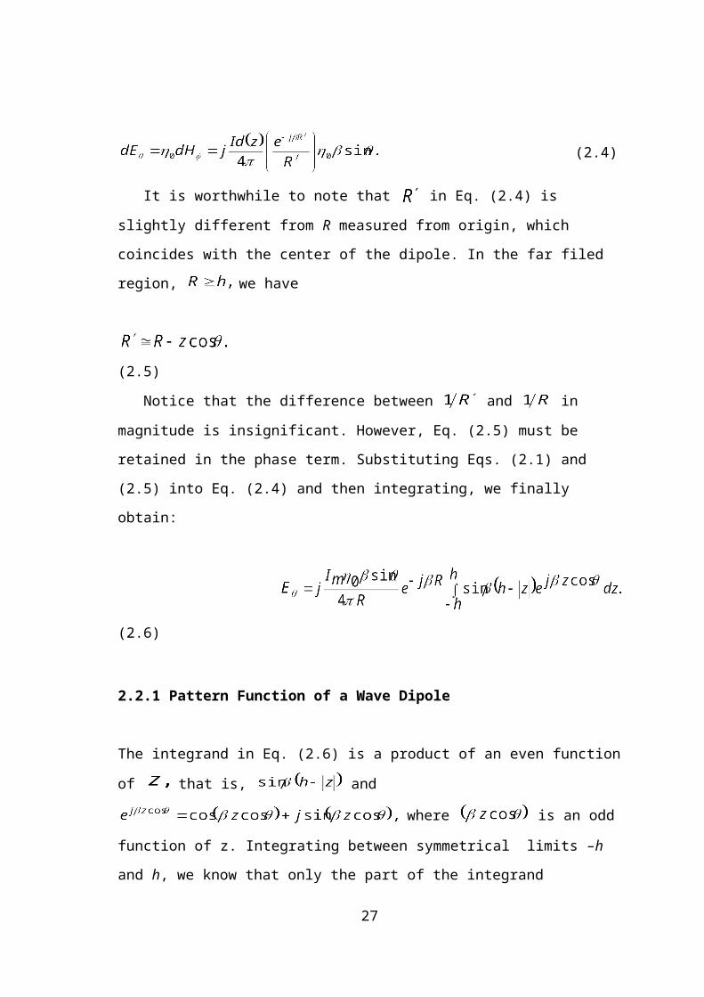
(2.4)

It is worthwhile to note that in Eq. (2.4) is slightly different from R measured

from origin, which coincides with the center of the dipole. In the far filed region, we have

(2.5)

Notice that the difference between and in magnitude is insignificant.

However, Eq. (2.5) must be retained in the phase term. Substituting Eqs. (2.1) and (2.5)

into Eq. (2.4) and then integrating, we finally obtain:

(2.6)

2.2.1 Pattern Function of a Wave Dipole

The integrand in Eq. (2.6) is a product of an even function of that is, and

where is an odd function of z.

Integrating between symmetrical limits –h and h, we know that only the part of the

integrand containing the product of two even function of z,

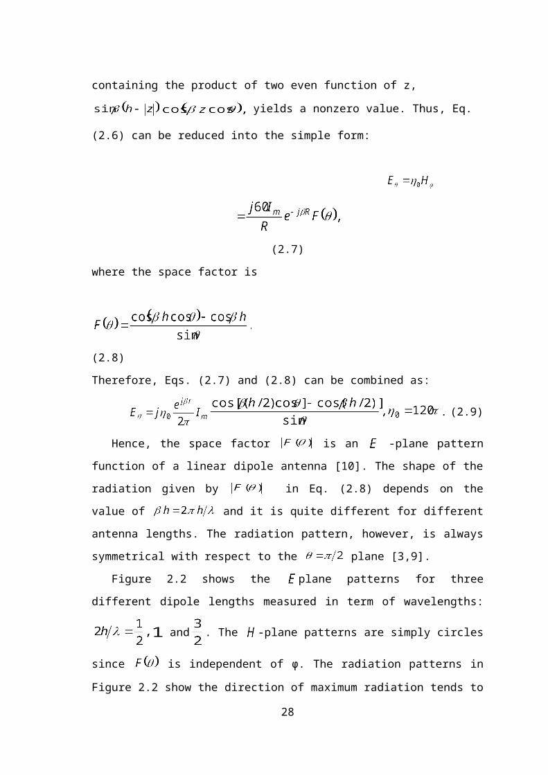
yields a nonzero value. Thus, Eq. (2.6) can be reduced into the simple form:

(2.7)

where the space factor is

(2.8)

Therefore, Eqs. (2.7) and (2.8) can be combined as:

18

. (2.9)

Hence, the space factor is an -plane pattern function of a linear dipole

antenna [10]. The shape of the radiation given by in Eq. (2.8) depends on the

value of and it is quite different for different antenna lengths. The radiation

pattern, however, is always symmetrical with respect to the plane [3,9].

Figure 2.2 shows the plane patterns for three different dipole lengths measured in

term of wavelengths: and . The -plane patterns are simply circles since

is independent of φ. The radiation patterns in Figure 2.2 show the direction of

maximum radiation tends to shift away from plane when the dipole length

approaches [9].

The half-wave dipole antenna of length is of a particular practical

importance because of its desirable pattern and impedance characteristics. Therefore we

have for the half wave dipole antenna.

(a) (b)

19

(c)

Figure 2.2 -Plane Radiation Patterns for Center-Fed Dipole Antennas [9].

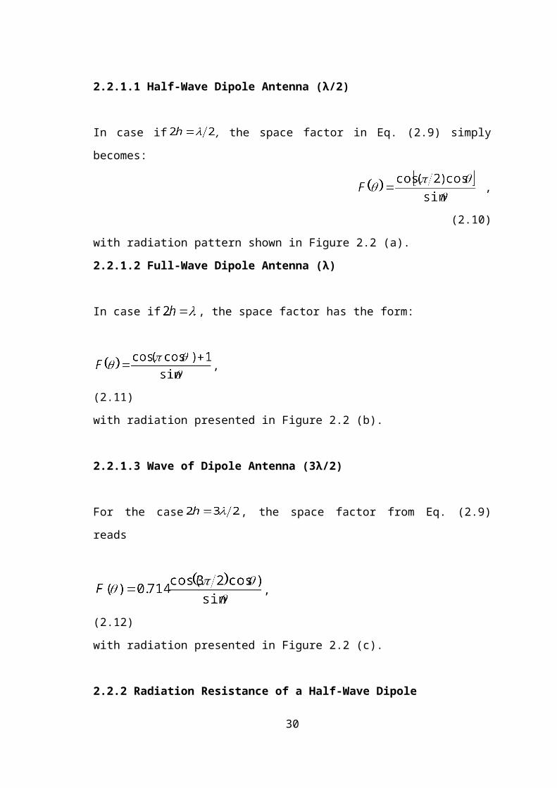
2.2.1.1 Half-Wave Dipole Antenna (λ/2)

In case if , the space factor in Eq. (2.9) simply becomes:

, (2.10)

with radiation pattern shown in Figure 2.2 (a).

2.2.1.2 Full-Wave Dipole Antenna (λ)

In case if , the space factor has the form:

, (2.11)

with radiation presented in Figure 2.2 (b).

2.2.1.3 Wave of Dipole Antenna (3λ/2)

For the case , the space factor from Eq. (2.9) reads

, (2.12)

with radiation presented in Figure 2.2 (c).

2.2.2 Radiation Resistance of a Half-Wave Dipole

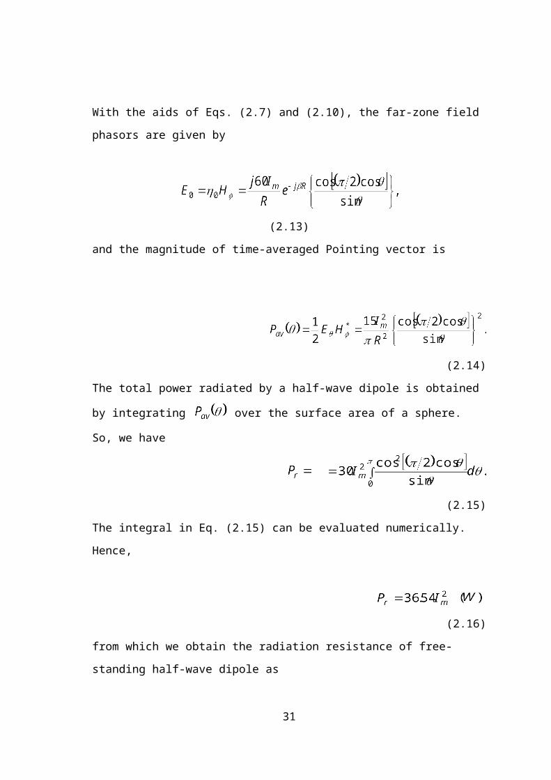
With the aids of Eqs. (2.7) and (2.10), the far-zone field phasors are given by

(2.13)

and the magnitude of time-averaged Pointing vector is

(2.14)

20

The total power radiated by a half-wave dipole is obtained by integrating over

the surface area of a sphere. So, we have

(2.15)

The integral in Eq. (2.15) can be evaluated numerically. Hence,

(2.16)

from which we obtain the radiation resistance of free-standing half-wave dipole as

(2.17)

Neglecting losses, the input resistance of a thin half dipole equals 73.1(Ω) and that

the input reactance is small positive number that can be made to vanish when the

dipole length is adjusted to slightly shorter than [9].

2.2.3 Directivity of a Half-Wave Dipole Antenna

The directivity of a half-wave dipole antenna can be calculated by using Eq. (1.4) as:

(2.18)

where

(2.19)

The directive value in Eq. (2.18) corresponds to or referring to an

omnidirectional radiator [9].

The criterion of beam width, although adequate and convenient in many situations,

it does not always provide a sufficient description of the beam characteristics. When

beams have different shapes. An additional description may be given by measuring the

width of the beam at several points, as an example, -3 dB, -10 dB, at the nulls. Some

beams may have an asymmetric shape [11].

2.3 Dipole Characteristics

21

Dipole characteristics comprise the following terminologies: frequency versus

length, feeder line, radiation pattern. These topics are explained in the followings.

2.3.1 Frequency Versus Length

Dipoles that are much smaller than the wavelength of the signal are called Hertzian,

short, or infinitesimal dipoles. These have a very low radiation resistance and a high

reactance, making them inefficient, but they are often the only available antennas at

very long wavelengths. In general, the term dipole usually means a half-wave dipole

(center-fed). A half-wave dipole is cut to length according to the formula

(2.20)

where is the length in feet and is the frequency in [8]. This is because the

impedance of the dipole is resistive pure at about this length. The metric formula is

(2.21)

the length is in meters. The length of the dipole antenna is about 95% of half a

wavelength at the speed of light in free space [8].

2.3.2 Radiation Patterns

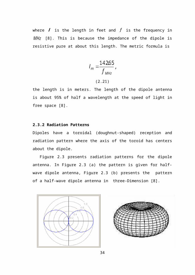
Dipoles have a toroidal (doughnut-shaped) reception and radiation pattern where the

axis of the toroid has centers about the dipole.

Figure 2.3 presents radiation patterns for the dipole antenna. In Figure 2.3 (a) the

pattern is given for half-wave dipole antenna, Figure 2.3 (b) presents the pattern of a

half-wave dipole antenna in three-Dimension [8].

22

(a) (b)

Figure 2.3 Radiation Patterns in Dipole Antenna in Free Space [8].

Furthermore, Table 2.1 shows the gain of the dipole antenna for different wavelengths

for free space.

Table 2.1 Gain of the Dipole Antennas [8].

Length (L ) in ( ) Gain Gain (dB)

1 1.50 1.76dB

0.5 1.64 2.15dB

1.0 1.80 2.55dB

1.5 1.80 3.01dB

2.0 2.30 3.62dB

3.0 2.80 4.47dB

4.0 3.50 5.44dB

8.0 7.10 8.51dB

2.3.3 Feeder Line

Ideally, a half-wave dipole antenna (λ/2) should be fed with a balanced line matching

the theoretical Ω impedance of the antenna. A folded dipole uses a Ω balanced

feeder line. Many people have had success in feeding a dipole directly with a coaxial

cable feed rather than a ladder-line.

However, coaxial cable is not symmetrical and thus not a balanced feeder. It is

unbalanced, because the outer shield is connected to earth potential at the other end.

When a balanced antenna such as a dipole is fed with an unbalanced feeder, common

mode currents can cause the coaxial cable line to radiate in addition to the antenna itself,

and the radiation pattern may be asymmetrically distorted This can be remedied with

the use of a balun where balun is a passive electronic device that converts between

balanced and unbalanced electrical signals. They often also change impedance. Baluns

23

can take many forms and their presence is not always obvious. They always involve

some form of electromagnetic coupling [8].

2.4 Types of Dipole Antennas

Various types of dipole antennas are presented in Figure 2.4. Dipole antennas are

distinguished by their flexibility. The most common variations include the inverted V or

sometimes is called the drooping dipole as in Figure 2.4 (a); multiband parallel dipole

shown in Figure 2.4 (b); sloping dipole in Figure 2.4 (c); folded dipole in Figure 2.4 (d)

and trap dipole in Figure 2.4 (e). Inverted-V dipoles are probably more common than

flat-top versions. As we might expect, the inverted V gets its name from its shape. The

main advantages of inverted V are that they need only one high support, and that one

can get more total wire into the same horizontal space using this configuration. This is

often an important advantage on the lower-frequency bands, where real estate and

support height suitable for putting up a full-size dipole are at a premium.

Inverted V usually work almost as well as horizontal flat-top dipoles when the

dipole's height is the same as the feed-point height of an inverted V. Another common

dipole configuration is the multiband parallel version, as shown in Figure 2.4 (b). The

multiple dipole elements are fed at the same point, with a single feed line, and supported

by spacers attached to the longest dipole element. The main advantage of parallel

dipoles is multiband coverage with resonant elements on each band, allowing the use of

a single coaxial feed line for several bands without the need for an antenna tuner.

However, an inherent disadvantage of parallel dipoles is narrower bandwidth than single

dipoles. The sloping dipole antenna as in Figure 2.4 (c) offers directivity in sloping

direction.

The dipole element pointing up should be connected to the center conductor of the

coaxial cable. This antenna is for vertical polarization via ground wave and long-haul

ionospheric propagation, and requires just one point of suspension.

Two other fairly popular dipole variations are the trap dipole and the folded dipole.

Traps are tuned circuits (consisting of inductance and capacitance) that electrically

isolate the inner and outer sections of the antenna at certain frequencies, providing

multiband resonant coverage from a single antenna.

24

At a traps resonant frequency, it presents high impedance and therefore isolates the

outer segments of the dipole, making the antenna electrically shorter than it is

physically. At frequencies below the traps resonance, it has a low impedance, which

makes it transparent to radio frequency (RF) (i.e., it doesn’t isolate any part of the

antenna). Traps are not used only in dipoles: Trap Yagi beams and verticals are also

popular.

Folded dipoles are a bit less common in Amateur Radio use. They use full-length

parallel wires shorted at the ends, and have feed-point impedances that provide good

matches to balanced feed lines. FM-broadcast receivers usually use folded dipoles made

from TV twin lead [12].

(a) Inverted V Dipole. (b) Multiband Parallel Dipole.

(c) Sloping Dipole.

(d) Folded Dipole.

25

Feed Point

Support

Feed Point

Feed

Point

Feed Point

Feed Point

(e) Trap Dipole.

Figure 2.4 Various Dipole Antennas [12,13].

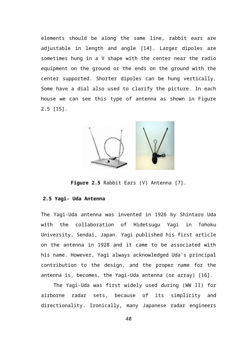
The most common dipole antenna is the rabbit ears (V) type used with televisions.

While theoretically the dipole elements should be along the same line, rabbit ears are

adjustable in length and angle [14]. Larger dipoles are sometimes hung in a V shape

with the center near the radio equipment on the ground or the ends on the ground with

the center supported. Shorter dipoles can be hung vertically. Some have a dial also used

to clarify the picture. In each house we can see this type of antenna as shown in Figure

2.5 [15].

Figure 2.5 Rabbit Ears (V) Antenna [7].

2.5 Yagi- Uda Antenna

The Yagi-Uda antenna was invented in 1926 by Shintaro Uda with the collaboration of

Hidetsugu Yagi in Tohoku University, Sendai, Japan. Yagi published his first article on

the antenna in 1928 and it came to be associated with his name. However, Yagi always

acknowledged Uda's principal contribution to the design, and the proper name for the

antenna is, becomes, the Yagi-Uda antenna (or array) [16].

The Yagi-Uda was first widely used during (WW II) for airborne radar sets,

because of its simplicity and directionality. Ironically, many Japanese radar engineers

were unaware of the design until very late in the war, due to inter-branch fighting

between the Army and Navy.

Arrays can be seen on the nose cones of many (WWII) aircraft, notably some

versions of the German Junkers Ju 88 fighter-bomber and the British Bristol Beau

fighter night-fighter and Short Sunderland flying-boat [16].

26

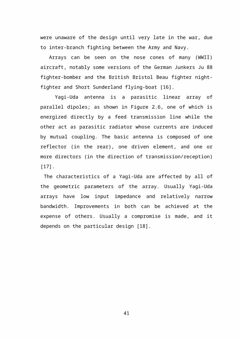
Yagi-Uda antenna is a parasitic linear array of parallel dipoles; as shown in

Figure 2.6, one of which is energized directly by a feed transmission line while the other

act as parasitic radiator whose currents are induced by mutual coupling. The basic

antenna is composed of one reflector (in the rear), one driven element, and one or more

directors (in the direction of transmission/reception) [17].

The characteristics of a Yagi-Uda are affected by all of the geometric parameters of the

array. Usually Yagi-Uda arrays have low input impedance and relatively narrow

bandwidth. Improvements in both can be achieved at the expense of others. Usually a

compromise is made, and it depends on the particular design [18].

Figure 2.6 Geometry of Yagi-Uda Array [18].

Further, the Yagi Uda antenna is a balanced traveling-wave structure, which has

high directivity, gain, and front-to-back ratio. It is considered to be balanced because

the voltage down the center of the antenna is constantly zero. As seen in Figure 2.6 the

Yagi-Uda consists of three sections: the reflector, the driven element, and the directors.

The reflector is a parasitic element placed, usually 0.1 to 0.25 wavelengths behind the

driven element. This causes the radiation from the driven element to be reflected toward

the front of the antenna. The driven element is the only active element on the antenna.

It is approximately one half of the wavelength of the operating frequency and is

27

Reflector Driven

Element

Director

attached to a feed-line. Often this feed-line is not matched in impedance or is

unbalanced. To match the antenna to the feed-line, a balun is often used [19].

The unbalanced line, such as coax, usually has no voltage at the outside and a

changing voltage down the center. A balun is a device used to attach a balanced system

(antenna) to an unbalanced system (line), which is placed between the antenna and the

feed-line. If a balun is not used, the voltages on the two halves of the driven element

may be different. This could result in some unpredictable changes to the radiation

pattern of the antenna. In front of the driven elements are the directors. When the

number of directors increase, the directivity, gain, and front to back ratio increases.

However, this is often done at the expense of adding side-lobes.

The ideal version of the Yagi-Uda has all directors and the driven element one-half

wavelength long and spaced one-quarter wavelength apart. The elements are held in

place by a boom, which attaches to the center of each element.

This should not affect the radiation pattern because; the current at the center of each

element is a constant zero. However, it is often necessary to compensate by using metal

boom [20]. Directional antennas, or beam antennas, have two big advantages over

dipole and vertical antennas. The first advantage is that a beam antenna concentrates

most of its transmitted signal in one compass direction. Directivity or gain is provided

in the direction the antenna is pointed. This makes the signal sound stronger to other

operators and vice versa, when compared with non-directional antennas. The second

important advantage of beam antennas is the reduction in the strength of signals coming

from directions other than where the point is. By reducing the interference from stations

in other directions the operating enjoyment in the desired direction can be increased.

Beam antennas find their most use on 15 and 10 meters and are very popular on the

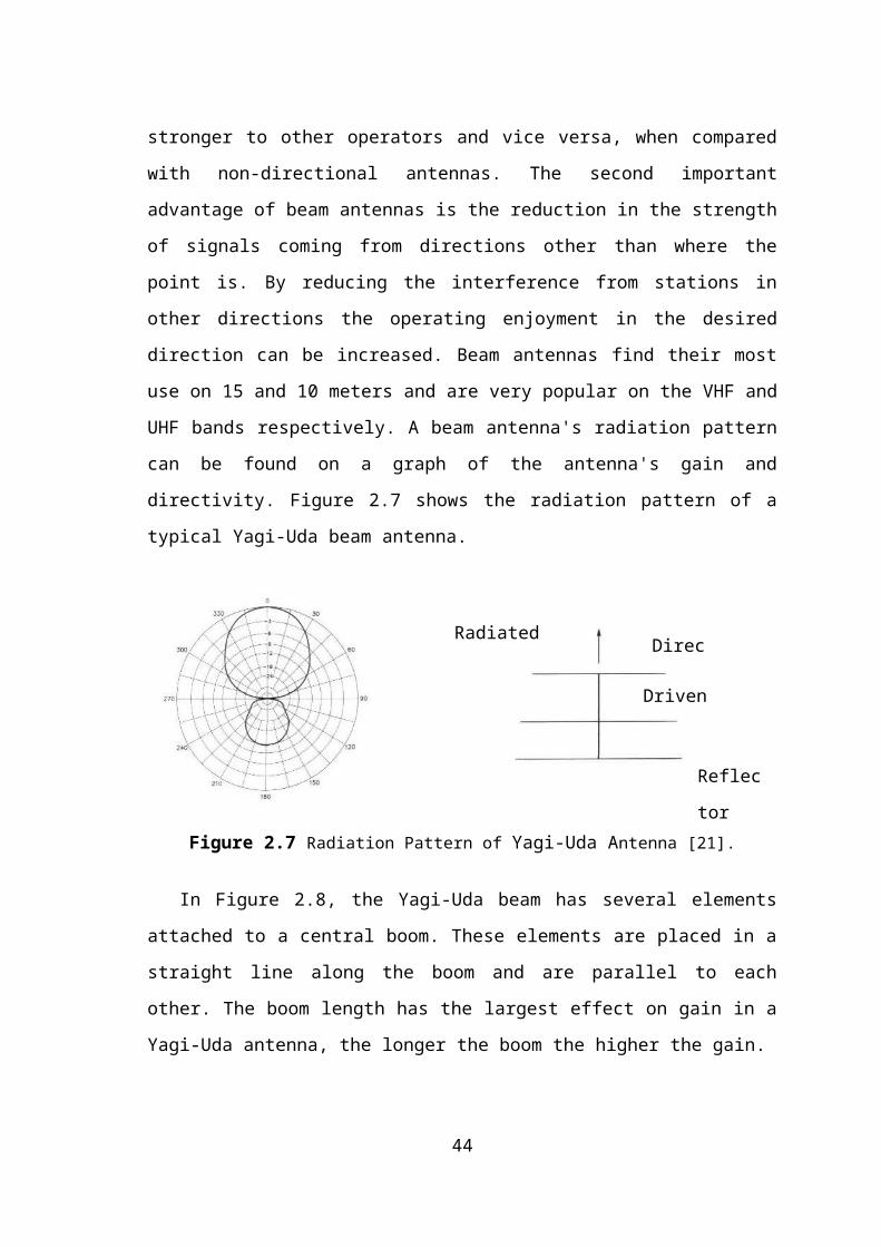
VHF and UHF bands respectively. A beam antenna's radiation pattern can be found on a

graph of the antenna's gain and directivity. Figure 2.7 shows the radiation pattern of a

typical Yagi-Uda beam antenna.

28

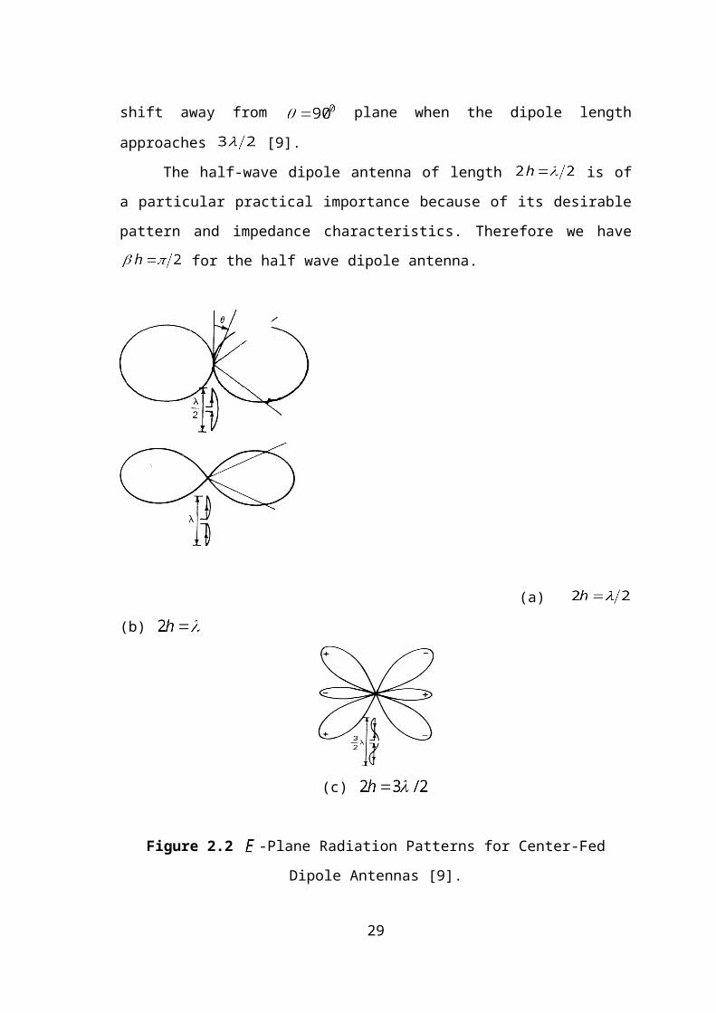
Figure 2.7 Radiation Pattern of Yagi-Uda Antenna [21].

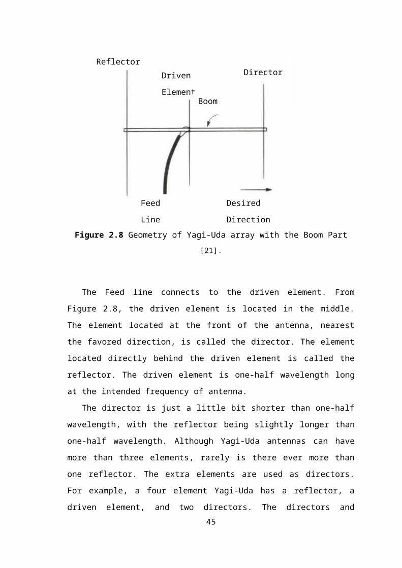
In Figure 2.8, the Yagi-Uda beam has several elements attached to a central boom.

These elements are placed in a straight line along the boom and are parallel to each

other. The boom length has the largest effect on gain in a Yagi-Uda antenna, the longer

the boom the higher the gain.

Figure 2.8 Geometry of Yagi-Uda array with the Boom Part [21].

The Feed line connects to the driven element. From Figure 2.8, the driven element

is located in the middle. The element located at the front of the antenna, nearest the

favored direction, is called the director. The element located directly behind the driven

29

DirectorDriven Element

Reflector

Boom

Feed Line Desired Direction

Radiated SignalDirector

Driven Element

Reflector

element is called the reflector. The driven element is one-half wavelength long at the

intended frequency of antenna.

The director is just a little bit shorter than one-half wavelength, with the reflector

being slightly longer than one-half wavelength. Although Yagi-Uda antennas can have

more than three elements, rarely is there ever more than one reflector. The extra

elements are used as directors. For example, a four element Yagi-Uda has a reflector, a

driven element, and two directors. The directors and reflectors are also known as

parasitic elements, because they are not fed directly.

The direction of maximum radiation is from the reflector on through the driven

element to the director in a beam antenna. For a single-band beam on six or two meters,

use a TV mast, hardware and rotator can be used in order to change the directions of the

antenna [21].

In Table 2.2, Yagi-Uda antenna parameters were given by stutzman [1], where

different numbers of elements increasing from 3 to 7 were given as well, gain and input

impedance. The frequency was used as 118 and the diameter of the conductor was

. Figure 2.9 shows that as the number of elements increases, the gain of the

antenna increase which it will affect in the performance of the antenna.

Table 2.2 Characteristics of Equally Spaced Yagi-Uda Antennas [1].

3 0.25 0.479 0.453 0.451 9.4 5.6 22.3+ j15

4 0.20 0.503 0.474 0.463 9.3 7.5 5.6+ j20.7

4 0.25 0.486 0.463 0.456 10.40 6 10.3+ j23.5

4 0.3 0.475 0.453 0.446 10.7 5.2 25.8+ j23.5

5 0.15 0.505 0.476 0.456 10 13.1 9.6+ j13

5 0.20 0.486 0.462 0.449 11 9.4 18.4+ j17.6

5 0.25 0.477 0.451 0.442 11 7.4 53.3+ j6.2

6 0.20 0.482 0.456 0.437 11.2 9.2 51.3 + j1.9

6 0.3 0.472 0.449 0.437 11.6 6.7 61.2+ j7.7

7 0.20 0.489 0.463 0.444 11.8 12.6 20.6+ j16.8

7 0.25 0.477 0.454 0.434 12 8.7 57.2+ j1.9

30

Here , denotes to number of elements, is the spacing wavelength between the

driver and directors, is the length of the reflector, is the length of the driver, is

the length of the directors, is the gain of the Yagi-Uda antenna, is the front to

back ratio and is the input impedance of the antenna.

Figure 2.9 Gain Versus Number of Elements [1].

2.6 Summary

This chapter introduced the radiation fields and characteristic properties of an elemental

electric dipole, and then discussed the finite-length thin linear antennas of which the

half-wave dipole antenna is an important special case. The parameters associated with

linear dipole antennas; such as current distribution on center-fed thin linear dipole

antennas, far-zone field intensities, pattern function, the radiation resistance and

directivity of a center-fed linear half-wave dipole antenna have been investigated.

Furthermore, as one of the applications to the linear dipole antenna, the Yagi-Uda

antenna has been studied, explaining the geometry and characteristics of this type of 31

N (Number of Elements)

Gain (dB)

antenna.

CHAPTER THREE

MODELING METHODS AND SOFTWARE FOR ANTENNAS

3.1 Overview

One of the significant contributions of computer technology to antenna design is the

improvement of modeling and simulation. Modeling and simulation are used in a wide

variety of applications, including management, science, and engineering. One can

model about any process, device, or any circuit that can be reduced mathematically.

The purpose of modeling is to do the design cheaply on the computer before

bending metal. If problems can be solved on a computer, the time and money would be

spared. Furthermore, modeling and simulation make it possible to look at more

alternatives and to gauge the effect of a change in an antenna design before the change

is made [22].

This chapter introduces the area of numerical simulation of electromagnetic properties. A short survey of three important numerical simulation methods used by the EM software which are, Method of Moment (MoM), Finite Difference Time Domain (FDTD) and Finite

Element Method (FEM), as well the main software that have been used on this thesis to obtain the numerical results will be explained in details.

3.2 Methods of Electromagnetic Simulators

32

Computational electromagnetic (EM) or electromagnetic modeling refers to the process

of modeling the interaction of electromagnetic fields with physical objects and the

environment.

It involves using computationally efficient approximations to Maxwell's Equations

and is used to calculate antenna performance, electromagnetic compatibility, radar cross

section and electromagnetic wave propagation when they are not in free space. Specific

part of computational EM deals with EM radiation scattered and absorbed by small

particles. EM can be used to model the domain generally by discretizing the space in

terms of grids (both orthogonal and non-orthogonal) and then solving the Maxwell's

equations at each point in the grid. Naturally, such discretization of the computational

space consumes computer memory and thus the solution of will take a longer time.

Large scale EM problems place computational limitations in terms of memory space,

and CPU time on the computer.

Generally, EM problems, as of 2007, are being simulated on super computers and

high performance clusters. There are three main EM simulation techniques used by the

software’s which are, Method of Moment (MoM), Finite-Difference Time Domain

(FDTD), and Finite Element Method (FEM) [23].

3.2.1 Method of Moment (MoM)

Method of moments (MoM) is based on the integral formulation of Maxwell's

equations; this basic feature makes it possible to exclude the air around the objects in

the discretization. The method is usually employed in the frequency domain but can also

be applied to time domain problems. In the MoM, integral based equations, describing

as an example the current distribution on a wire or a surface, are transformed into matrix

equations easily solved using matrix inversion. When using the MoM for surfaces a

wire-grid approximation of the surface can be utilizes. The wire formulation of the

problem simplifies the calculations and is often used for far field calculations.

The starting point for the theoretical derivation, is a linear (integral) operator, ,

involving the appropriate Green's function applied to an unknown function, ,

where is the known excitation function for the system as

(3.1)

33

For example, (3.1) can be the Pocklington Integral Equation, describing the current

distribution on a cylindrical antenna, written as

(3.2)

Then the wanted function, , can be expanded into as a series of known functions, ,

With unknown amplitudes, , resulting in

(3.3)

where are called basis (or expansion) functions. Figure 3.1 shows typical examples

on basis functions used in the MoM. To solve for the unknown amplitudes, n equations

are derived from the combination of (3.1) and (3.3) by the multiplication of n weighting

(or testing) functions, integrating over the wire length, and the formulation of a suitable

inner product. This results in the transformation of the problem into a set of linear

equations which can be written in matrix form as

(3.4)

where the matrices [Z], [I], and [V] are referred to as generalized impedance, current,

and voltage matrices and the desired solution for the current I is obtained by matrix

inversion. The unknown solution is expressed as a sum of known basis functions where

the weighting coefficients corresponding to the basic functions are determined for best

fit.

34

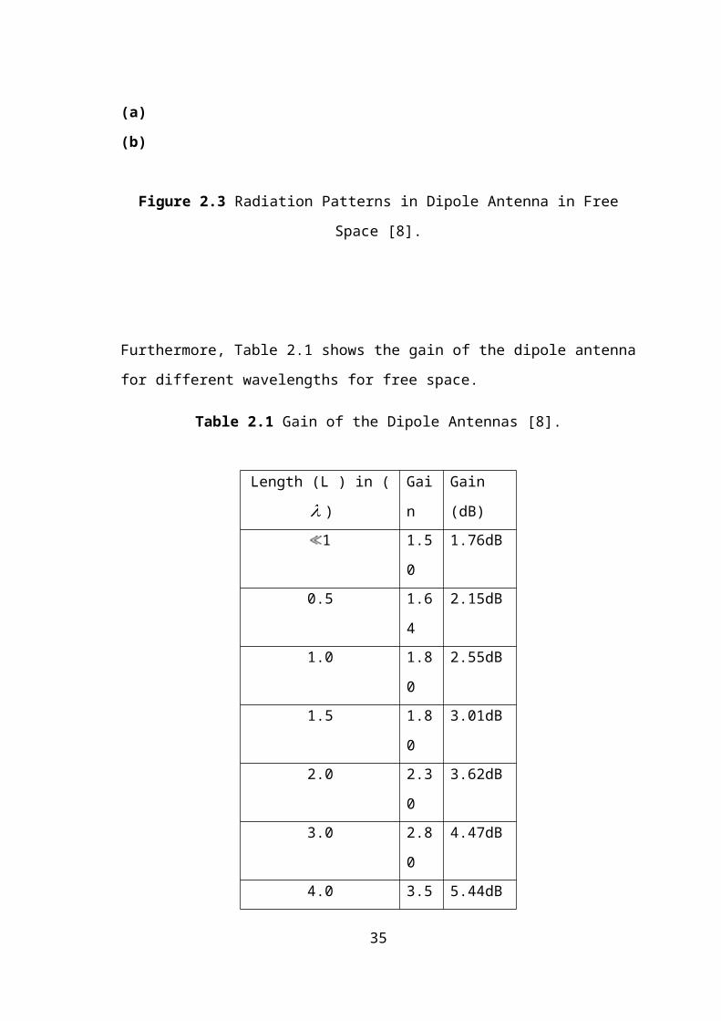
Figure 3.1: MoM Typical Basis Functions. (a) Piecewise Pulse Function, (b) Piecewise

Triangular Function, (c) Piecewise Sinusoidal Function [23].

The MoM delivers the result in system current densities and /or voltages at all

locations in the discretized structure and at every frequency point (depending on the

integral equation in (3.1)). To obtain the results in terms of field variables post

processing is needed for the conversion [23].

3.2.2 Finite-Difference Time Domain (FDTD)

FDTD is a full-wave, dynamic and powerful tool to solve Maxwell’s equations. This

method belongs to the general class of differential time domain numerical modeling

methods. Maxwell’s equations are modified to central differential equations and then

implemented in software. These equations are solved by finding the electric field at a

given instant of time, and then the magnetic field is solved at the next instant of time.

The process repeats itself until the model is resolved.

The FDTD is thus a useful numerical method suitable for modeling EM wave

propagation through complex media. Furthermore, it is ideal for modeling transient EM

fields in inhomogeneous media, such as complex geographical structures as it fits

relatively into the finite-difference grid. The absorbing boundary conditions can

truncate the grid to simulate an infinite region [23].

35

3.2.3 Finite Element Method (FEM)

FEM is a very powerful tool for solving complex engineering problems, the

mathematical formulation of which is not only challenging but also tedious. The basic

approach is to divide a complex structure into smaller sections of finite dimensions

known as elements. These elements are connected to each other via joints called nodes.

Each unique element is then solved independently of the others thereby drastically

reducing the complexity of solution. Hence, the final solution is then computed by

reconnecting all the elements and combining their solutions.

The FEM finds applications not only in EM but also in other branches of

engineering such as plane stress problems in mechanical engineering, vehicle

aerodynamics and heat transfer [23]. Appendix A presents the Maxwell’s equations in

integral and differential form.

Table 3.1 Main Features of the Most Commonly Used by EM Simulation Techniques

[23].

Method MoM FEM FDTD

Formulation Integral Differential Differential

Solution domain TD or FD TD or FD TD or FD

Advantages Cell flexibility Cell flexibility

complex Materials

Easy to robust

complex materials

Drawbacks Knowledge

computationally

heavy

Solve large liner

system

Cell non flexibility,

Storage

requirements

3.3 Simulation Software

36

Some of the main simulation software that are used in the present work will be

discussed.

3.3.1 Personal Computer Aided Antenna Design (PCAAD 5.0)

PCAAD 5.0 is the newest version of the most popular general purpose antenna

modeling software. It is a Windows-compatible antenna analysis, modeling, and design

software package. It also contains more than 40 separate routines treating various

antenna types like the wire antennas, aperture antennas, microstrip antennas, arrays, and

transmission lines and waveguides.

These routines are integrated into a menu-driven, user-friendly system allowing one

to quickly evaluate impedance and patterns for a wide variety of antenna types. Figure

3.2 shows a Screen Shot from PCAAD 5 [24].

Figure 3.2 Screen Shot from PCAAD 5 [24].

3.3.2 Numerical Electromagnetic Computation (NEC)

The NEC-4 software is the latest in the NEC series introduced by University of

California, The function of the NEC-4 software produces modeling of underground

37

radials, elements of varying diameter, and carefully constructs close-spaced parallel

wires [25].

3.3.2.1 NEC-2

It is a high-capability version of the NEC software, and can be used in the public

domain. This type is limited to antenna elements of constant diameter, although some

users base their software on NEC-2 that provides corrections for multi diameters [25].

3.3.2.2 EZNEC for Windows

EZNEC for Windows is available in both NEC-2 and NEC-4 versions. It offers 2-D and

3-D plots, 3-D plots with 2-D slicing, ground-wave output, stepped-diameter correction,

and various shortcuts to antenna modeling [26].

3.3.3 Makoto Mori Antenna Analysis (MMANA)

MMANA is an acronym used for the Makoto Mori Antenna Analysis Program. MANA

is an antenna analyzing tool based on the moment method introduced in Mini Numerical

Electromagnetic Code Version 3 (MININEC).

MININEC should not be confused with NEC, which is a largest antenna analysis

program written in FORTRAN and designed to run on main-frame computers. Early

versions of MININEC were written entirely in BASIC and the computation engine

source code was published as a PDS in MININEC Version 3.

That BASIC source code was ported to C++ and compiled to provide faster and

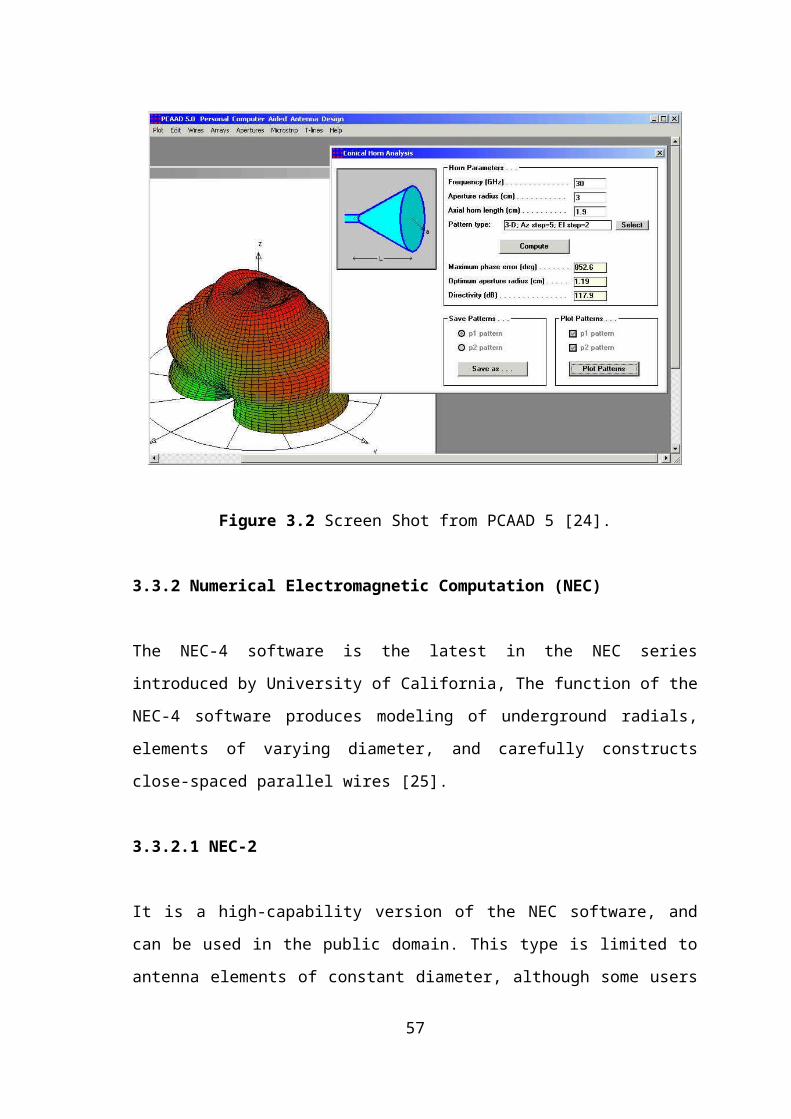
more memory-efficient computer execution. A graphical user interface was also added

to make MMANA much easier to use than MININEC version. Figure 3.3 shows a

Screen Shot from MMANA [27].

38

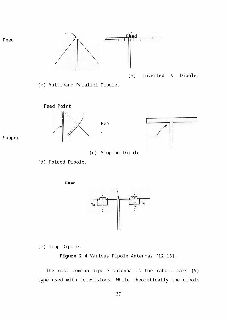
Figure 3.3 Screen Shot from MMANA [27].

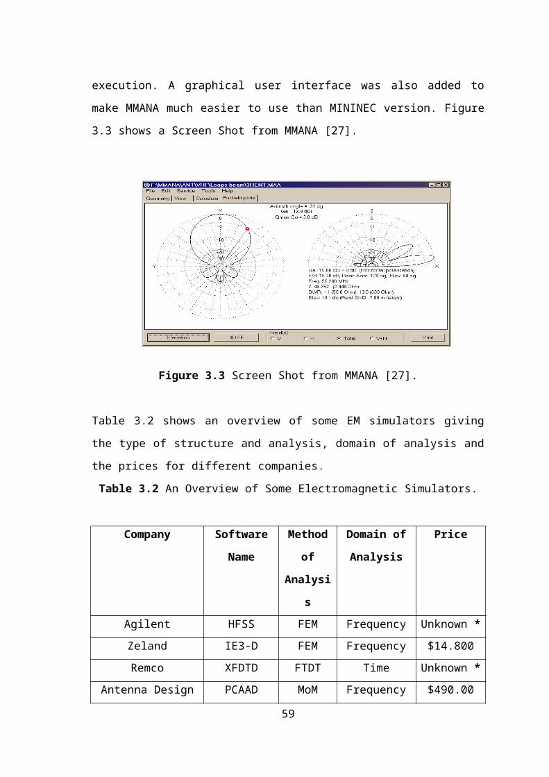
Table 3.2 shows an overview of some EM simulators giving the type of structure and

analysis, domain of analysis and the prices for different companies.

Table 3.2 An Overview of Some Electromagnetic Simulators.

Company Software

Name

Method

of

Analysis

Domain of

Analysis

Price

Agilent HFSS FEM Frequency Unknown *

Zeland IE3-D FEM Frequency $14.800

Remco XFDTD FTDT Time Unknown *

Antenna Design

Associates

PCAAD MoM Frequency $490.00

Computer Simulation

Technology

CST MoM Frequency $17.000

Antenna Software

W7EL

EZNEC Pro 5 MoM Frequency $650.00

MMANA MMANA MoM Frequency FREE

39

* Searching internet, the price is around $25.000 - $45.000.

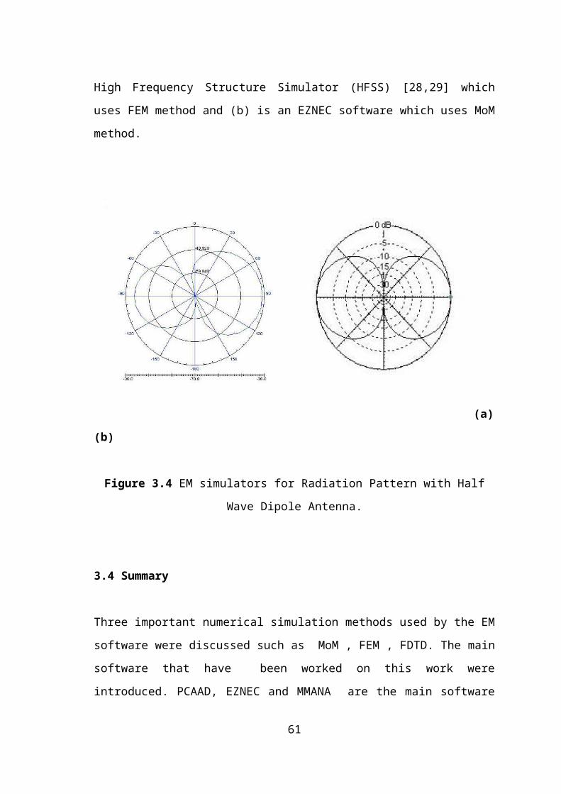
Figure 3.4 presents the radiation pattern of the half wave dipole antenna using

different software that use different methods, where (a) is the output of the gain from

High Frequency Structure Simulator (HFSS) [28,29] which uses FEM method and (b) is

an EZNEC software which uses MoM method.

(a) (b)

Figure 3.4 EM simulators for Radiation Pattern with Half Wave Dipole Antenna.

40

3.4 Summary

Three important numerical simulation methods used by the EM software were discussed such as MoM , FEM , FDTD. The main software that have been worked on this work were introduced. PCAAD, EZNEC and MMANA are the main software that are used in real life, and all of them are using the MoM method.

CHAPTER FOUR

SOME APPLICATIONS TO LINEAR DIPOLE ANTENNA

4.1 Overview

In this chapter, antenna software are used mainly to analyze various types of dipole

antennas such as half wave dipole antenna and rabbit ears. As a simple application,

Yagi-Uda antenna is considered. The analysis is based on theoretical part as well as the

results that are obtained during the simulations.

4.2 Introduction

Ultra-high frequency designates a band of EM waves with frequency between

and . and are the most commonly used frequency bands for

transmission of television signals. Modern mobile phones also transmit and receive

within the spectrum. Due to that, most of the results will be simulated by taking

into consideration the frequency and .

41

All the antenna software are simulated using HP Laptop, Intel Pentium M

processor, 1.80 GHz, 1 GB RAM, Mobile Intel, 915 GM/GMS, 910 GML Express

Chipset Family.

4.3 Dipole Antenna Simulations

Various types of antenna software are used to simulate the antennas such as:

MATLAB, PCAAD, MMANA and EZNEC.

4.3.1 MATLAB Simulations

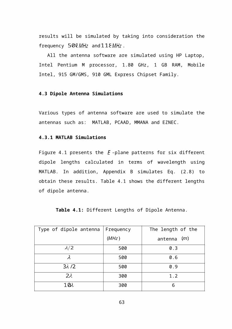
Figure 4.1 presents the -plane patterns for six different dipole lengths calculated in

terms of wavelength using MATLAB. In addition, Appendix B simulates Eq. (2.8) to

obtain these results. Table 4.1 shows the different lengths of dipole antenna.

Table 4.1: Different Lengths of Dipole Antenna.

Type of dipole antenna Frequency

The length of the antenna

500 0.3

500 0.6

500 0.9

300 1.2

300 6

42

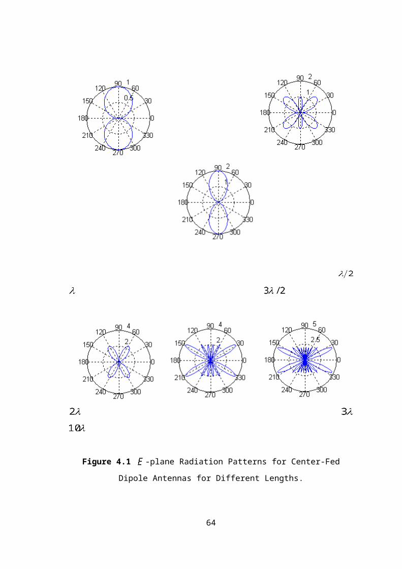
Figure 4.1 -plane Radiation Patterns for Center-Fed Dipole Antennas for Different

Lengths.

As seen in Table 4.1 the wavelength was calculated to find the length of the full

wave dipole antennas using Eq. (1.1). For instance the value of was find as 0.6 , so

half wave dipole antenna length will be 0.3 . In Figure 4.1, the -plane radiation

pattern for six different dipole lengths was plotted. Here this antenna consists of an

array of uniform dipoles and its radiation pattern has the property that . The

space factor = maximum in the first two cases when = and = , but not

in the third one, = , where the maximum shifts to . The -plane

radiation patterns are azimuthally symmetric circles since is independent of the

angle . If = , then the radiation pattern at plane is equal to zero.

Hence the contours depicted in Figure 4.1 are called lobes. The lobe in the direction

of the maximum is called the main lobe and the others are called side lobes, as the

43

length of the dipole increase the lobes will increase as in the case = . If a

compression is done for the present results with the ones given in Chapter 2, the same

results as in the theoretical part are obtained.

4.3.2 MMANA Simulations for Half Wave Dipole Antenna

The following procedure provides an antenna simulation. It investigates the dependence

of gain and feed point impedance on the length of a dipole in free space.

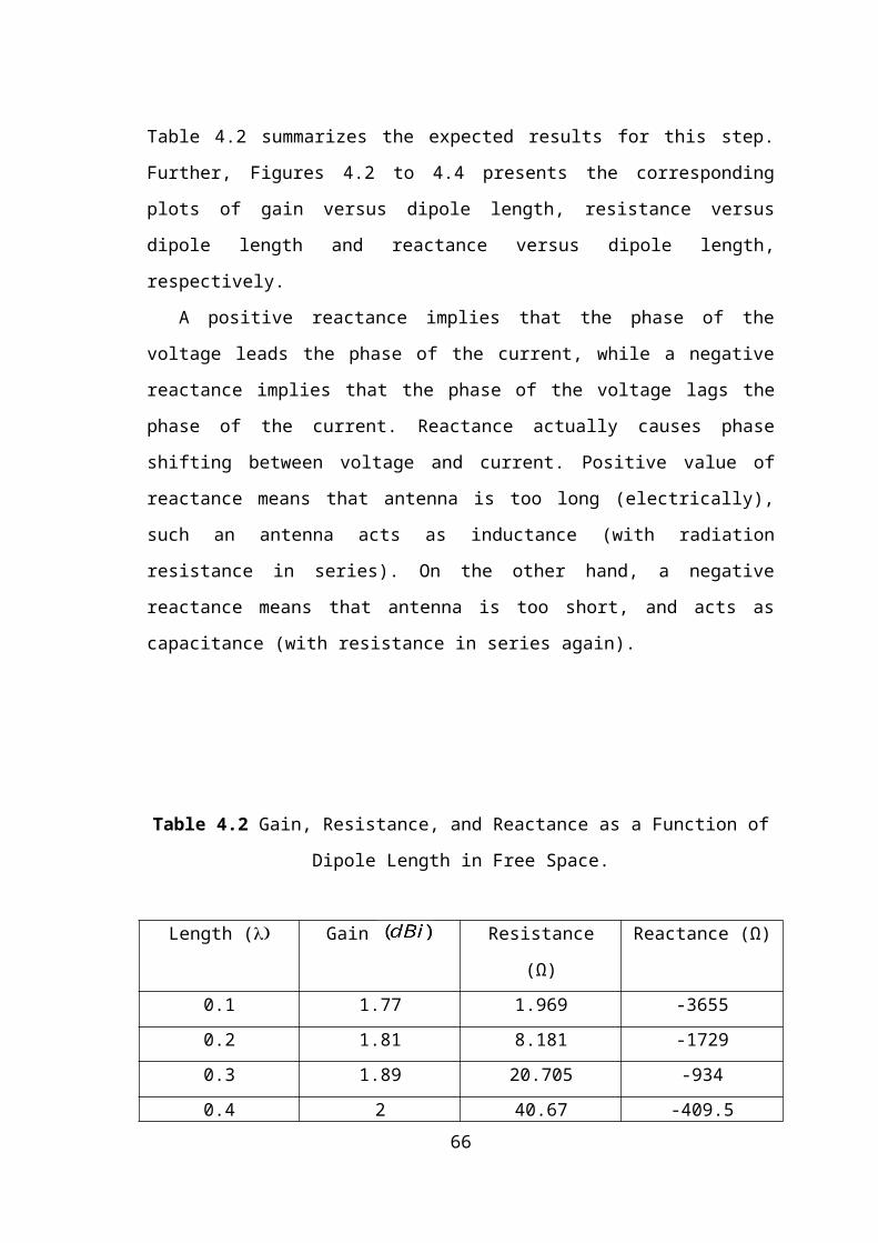
Table 4.2 summarizes the expected results for this step. Further, Figures 4.2 to 4.4

presents the corresponding plots of gain versus dipole length, resistance versus dipole

length and reactance versus dipole length, respectively.

A positive reactance implies that the phase of the voltage leads the phase of the

current, while a negative reactance implies that the phase of the voltage lags the phase

of the current. Reactance actually causes phase shifting between voltage and current.

Positive value of reactance means that antenna is too long (electrically), such an antenna

acts as inductance (with radiation resistance in series). On the other hand, a negative

reactance means that antenna is too short, and acts as capacitance (with resistance in

series again).

Table 4.2 Gain, Resistance, and Reactance as a Function of Dipole Length in Free

Space.

Length ( Gain Resistance (Ω) Reactance (Ω)

0.1 1.77 1.969 -3655

0.2 1.81 8.181 -1729

0.3 1.89 20.705 -934

0.4 2 40.67 -409.5

0.5 2.15 76.88 44.02

0.6 2.35 145.6 526.7

0.7 2.61 298 115944

0.8 2.94 757.4 2231

0.9 3.36 3447 4539

1 3.87 6374 -5440

1.5 3.53 110 49.65

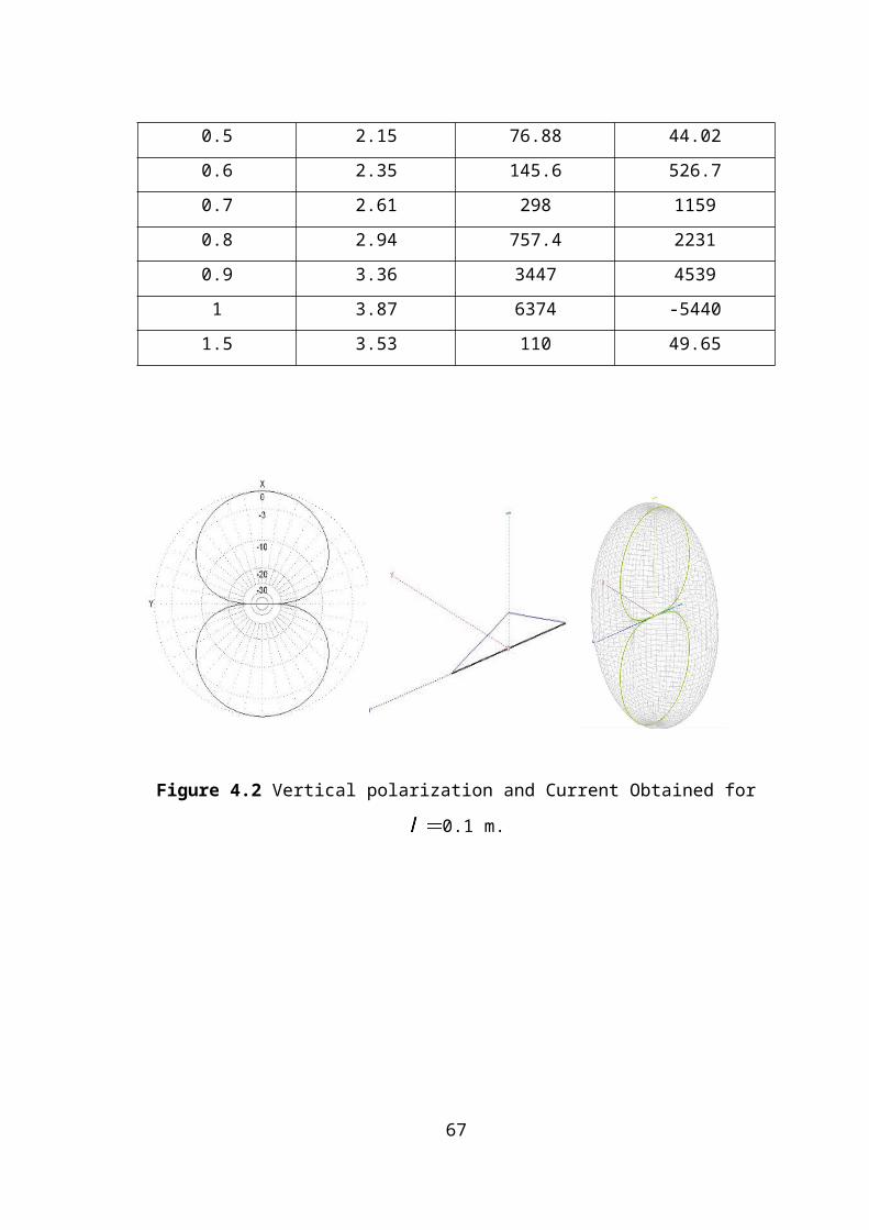
Figure 4.2 Vertical polarization and Current Obtained for 0.1 m.

Figure 4.3 Vertical Polarization and Current Obtained for 0.6 m.

45

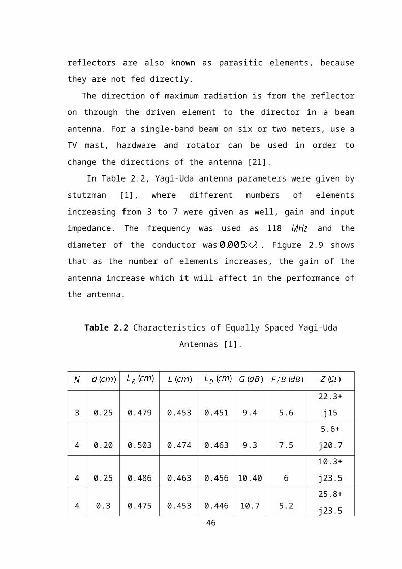
Figure 4.4 Vertical Polarization and Current Obtained for 1.5 m.

Figure 4.5 Current in Dipoles versus Length.

46

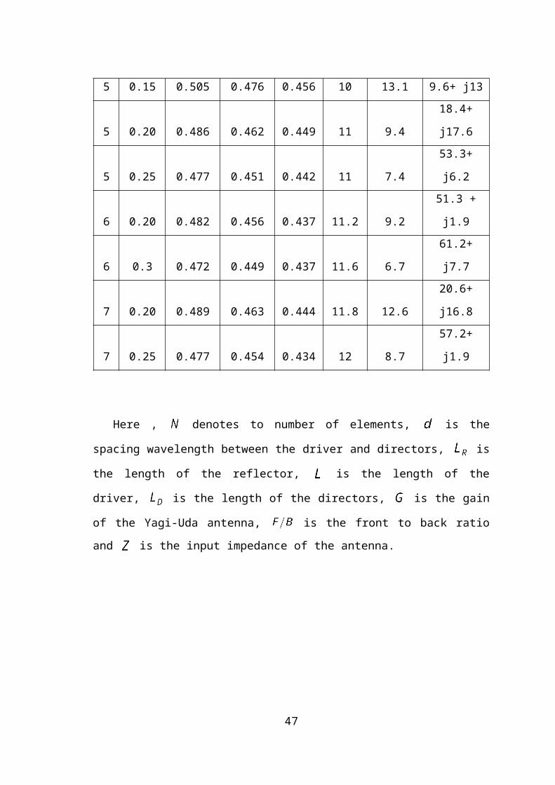
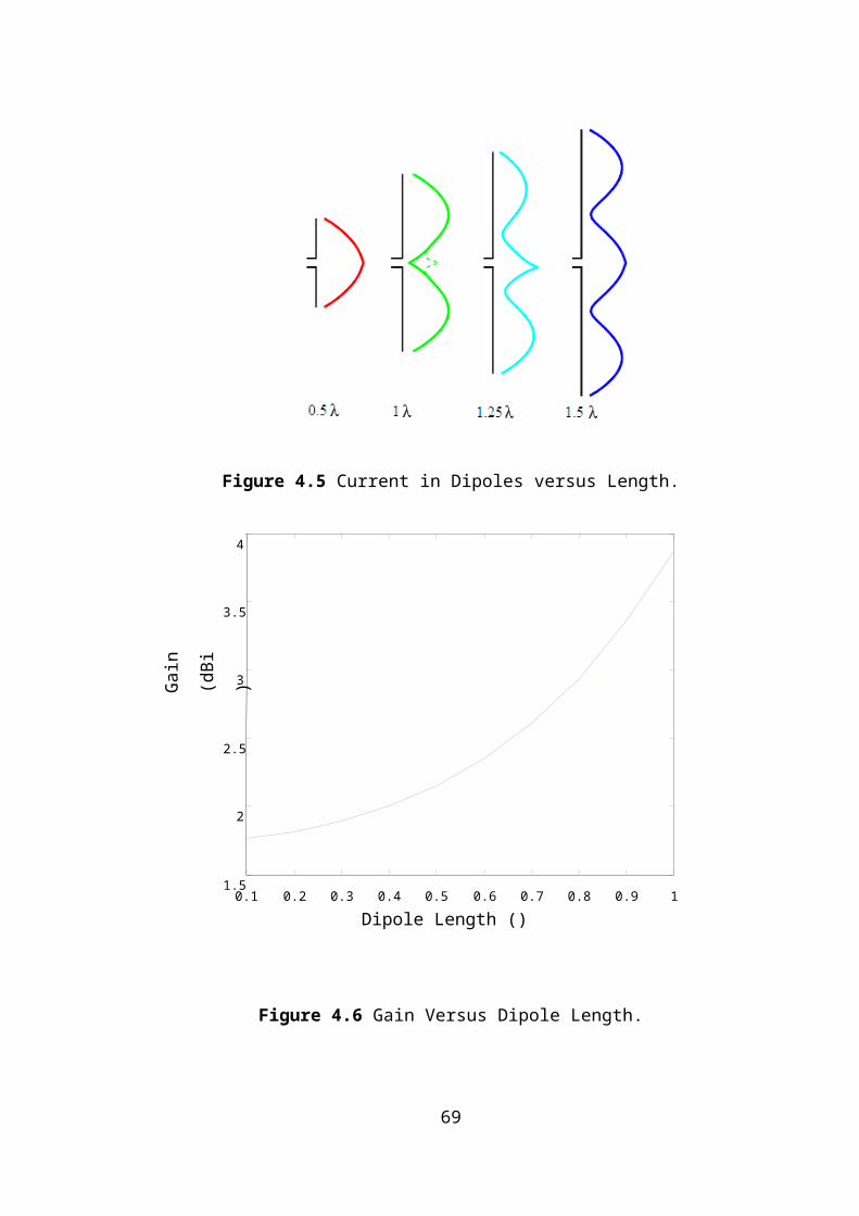
Figure 4.6 Gain Versus Dipole Length.

47

0.1 0.2 0.3 0.4 0.5 0.6 0.7 0.8 0.9 11.5

2

2.5

3

3.5

4

Dipole Length ()

Gai

n

(dB

i)

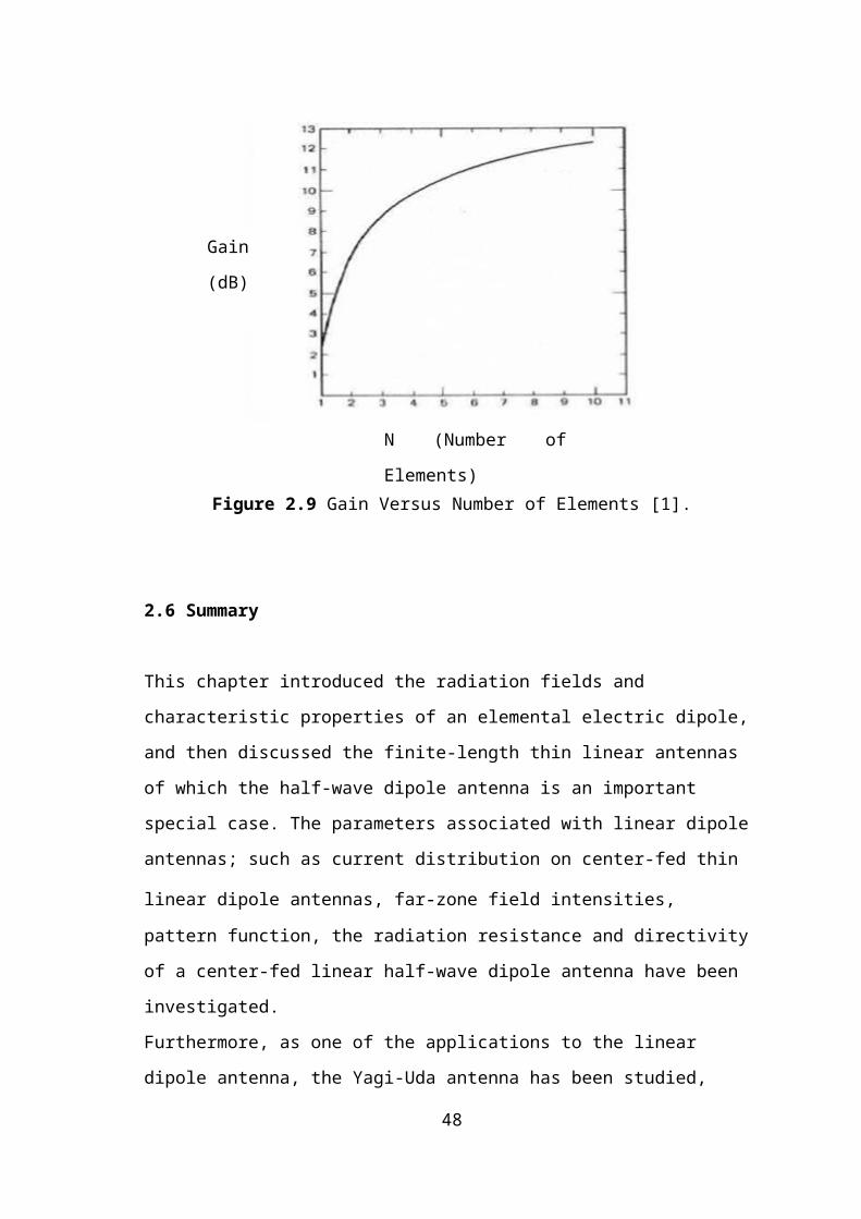
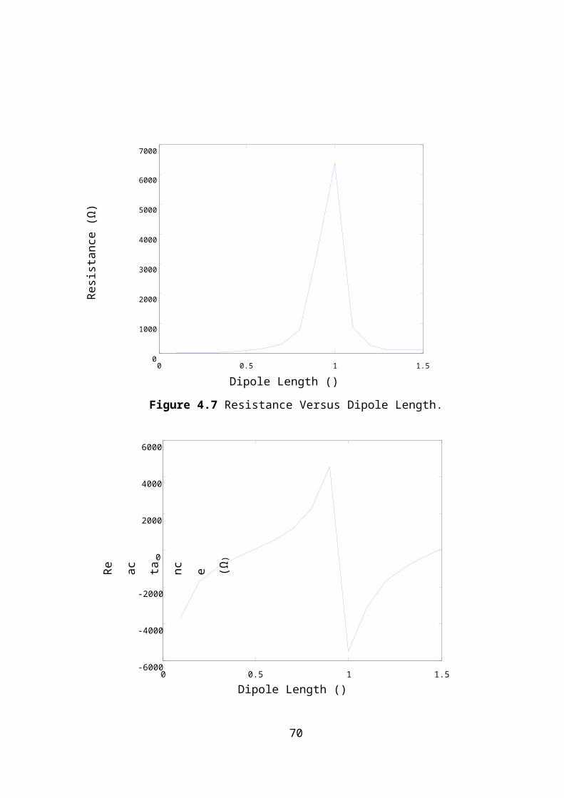
Figure 4.7 Resistance Versus Dipole Length.

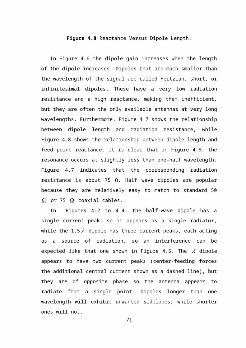
Figure 4.8 Reactance Versus Dipole Length.

48

0 0.5 1 1.50

1000

2000

3000

4000

5000

6000

7000

Dipole Length ()

0 0.5 1 1.5-6000

-4000

-2000

0

2000

4000

6000

Dipole Length ()

Res

ista

nce

(Ω)

Rea

ctan

ce

(Ω)

In Figure 4.6 the dipole gain increases when the length of the dipole increases.

Dipoles that are much smaller than the wavelength of the signal are called Hertzian,

short, or infinitesimal dipoles. These have a very low radiation resistance and a high

reactance, making them inefficient, but they are often the only available antennas at

very long wavelengths. Furthermore, Figure 4.7 shows the relationship between dipole

length and radiation resistance, while Figure 4.8 shows the relationship between dipole

length and feed point reactance. It is clear that in Figure 4.8, the resonance occurs at

slightly less than one-half wavelength. Figure 4.7 indicates that the corresponding

radiation resistance is about 75 Ω. Half wave dipoles are popular because they are

relatively easy to match to standard 50 or 75 coaxial cables.

In Figures 4.2 to 4.4, the half-wave dipole has a single current peak, so it appears

as a single radiator, while the 1.5 dipole has three current peaks, each acting as a

source of radiation, so an interference can be expected like that one shown in Figure 4.5.

The dipole appears to have two current peaks (center-feeding forces the additional

central current shown as a dashed line), but they are of opposite phase so the antenna

appears to radiate from a single point. Dipoles longer than one wavelength will exhibit

unwanted sidelobes, while shorter ones will not.

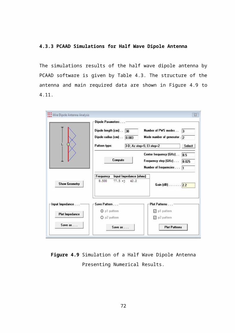
4.3.3 PCAAD Simulations for Half Wave Dipole Antenna

The simulations results of the half wave dipole antenna by PCAAD software is given by

Table 4.3. The structure of the antenna and main required data are shown in Figure 4.9

to 4.11.

49

Figure 4.9 Simulation of a Half Wave Dipole Antenna Presenting Numerical Results.

Figure 4.10 Radiation Pattern in Three Dimensions for Gain.

50

Figure 4.11 The - Plane Radiation Pattern of Half Wave Dipole Antenna.

Table 4.3 Simulating Results for the Half Wave Dipole Antenna by PCAAD.

( (

500 MHz 30 2.2 77.5 42.2

4.3.4 EZNEC and 4NEC2 Simulations for Half Wave Dipole Antenna

The simulations results of the half wave dipole antenna by 4NEC2 software are given

by Table 4.4. The structure of the antenna and main required data are presented in

Figures 4.12 – 4.13.

51

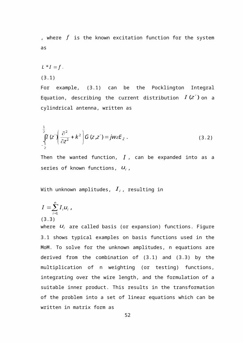
Figure 4.12 Structure of the Half Wave Dipole Antenna.

52

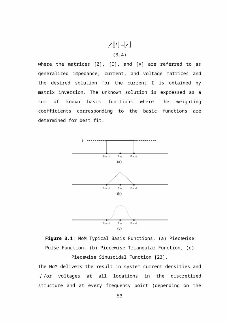
Figure 4.13 A Plot for the Simulated Structure by EZNEC and 4NEC2.

Table 4.4 The Obtained Results in Simulating the Half Wave Dipole Antenna by

EZNEC and 4NEC2.

500 MHz 30 2.16 85.3 48.2

It is shown, from Table 4.2 to 4.4, the Peak gain is 2.2 . All other parameters can

be seen as slightly elevated above the expected value. Adjustments to the radiation

boundary might provide more accuracy. The input resistance of the antenna is varying

from 76.88 to 85.3 as shown in these tables. According to the theoretical part the

gain should be 2.15 and the resistance is 73.1

In regards to the results that are obtained impedance is in good agreement as they

are relatively easy to match with standard 50 or 75 coaxial cables.

53

4.4 PCAAD Simulations to Rabbit Ears (V) Antenna

In this section the rabbit ears antenna is simulated using different angles and length

in order to check the value of the gain. Figures 4.14 to 4.15 represent the rabbit ears

with different lengths and angles fixing the frequency to be 500 .

(a)

(b)

(c)54

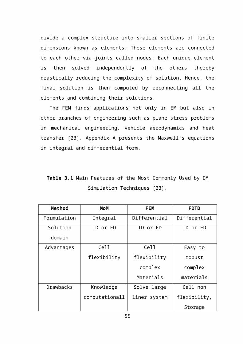
Figure 4.14 The Radiation Pattern of Rabbit Ears with 30 cm and .

Figure 4.14 (a) represents the simulated results of the data which was entered, (b)

shows the 3-D of the pattern radiation of the rabbit ears and (c) is the Polar pattern

radiation of this antenna.

55

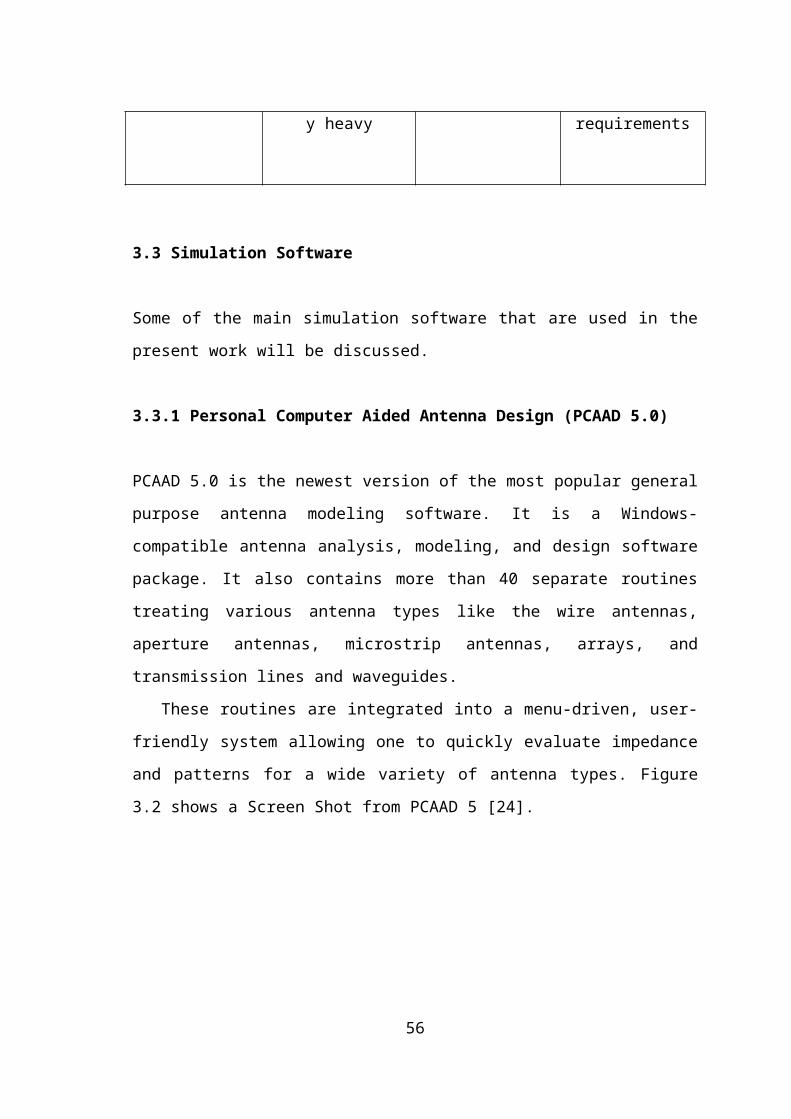
Figure 4.15 The Radiation Pattern of Rabbit Ears with 30 cm and .

Table 4.5 The Gain of the Rabbit Ears (V) Antenna using Different Angles and

Lengths.

(cm) (Degree)

30 170 4

30 30 3.1

20 170 2.5

20 30 1

15 170 2.2

15 70 1.6

10 170 1.9

Table 4.5 presents the gain values for various lengths and angles for received rabbit

ear antenna. The polarization of the TV signals rotates as it bounces off things

56

(buildings, the ground, etc), and so it has to match the receive antenna polarization of

the TV signals. Rabbit Ears are just a simple adjustable Dipole. Adjusting the length of

each leg will make the antenna resonant on different frequencies. Adjusting the angle

between the two "ears" will affect the radiation pattern.

Making a smaller angle the antenna will be behaving more like an isotropic

radiator i.e. receives signals all around with almost no attenuation. If angle is increased,

the pattern will become a straight dipole, having deep nulls at each end. This can be

very handy when trying to remove unwanted signals. Feeding impedance will decrease

when decreasing the angle. From all the results, analysis can be done to the simulated

results according to Eqs. (1.13) and (1.14), which gives the general formula for

calculating gain with respect to antenna size. As frequency increases wavelength

decreases, Gain is inversely proportional to wavelength, so as frequency increases gain

also increases.

Furthermore, the gain is directly proportional to Area of the aperture so as the area

of the antenna increases gain also increases. Noting that gain is inversely proportional to

beam width. As side lobe level increases, the signals will be spitted in the unwanted

direction and signal strength at the required direction will be less.

Table 4.6 compares between the results that were obtained from using different

software’s which were presented in Table 4.(2-3-4).

Table 4.6 Comparing of Different Software’s using Same Parameters and Same Method

( ( Name of Program

500 MHz 30 2.2 77.5 42.2 PCAAD

500 MHz 30 2.16 85.3 48.2 EZNEC

500 MHz 30 2.15 76.88 44.02 MMANA

500 MHz 30 2.15 75 50 Theoretically

As it is presented in Table 4.6 the range of the frequency and the main parameters were

same as well the Computational electromagnetic (EM) method is same (MoM), but the

obtained results where different comparing with the theoretical part. The reasons for

57

that is to the main characters of MoM method, the difference is in the implementation of

the MOM (speed reasons). The MoM has many integrals, so some of the calculations

for these integrals is not very accurate. These differences are very visible for impedance

calculation, and not very important of radiation patterns.

The calculations are based on approximations, which each company gives at their

choice, which makes the result different. When integrals equations is solved the

calculations of the computer uses approximate values, so that’s why each software has

its own values. So segments, thickness and other parameters also should be taken in

account in order to get accrue answers. Integration must be precise enough to give a

stable system of linear equations (which basically means that if the user increases the

accuracy of integration its no longer influences the results significantly).

4.5 Simulations of Yagi-Uda Antenna

As an application to dipole antennas, Table 2.2 will be used in order to simulate the

Yagi-Uda antenna by using different software. In order to simulate a Yagi-Uda antenna

for 3 elements, and frequency , the following parameters will be calculated [1]:

Element Number,

Radius of each element,

Reflector length,

Feeder length,

Directors length,

Space between directors,

4.5.1 PCAAD Simulations of Yagi-Uda Antenna

58

Figures 4.16, 4.17 show the numerical results of the antenna. Furthermore, Table 4.6,

the gain and input impedance are given starting from 3 elements to 7 elements of Yagi-

Uda antenna.

Figure 4.16 Simulations of Yagi-Uda Antenna with Elements =3.

59

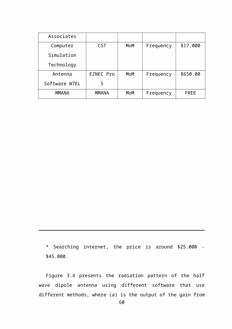
Figure 4.17 Simulation of Yagi-Uda Antenna with Elements =5.

Figure 4.18 shows the radiation pattern for Yagi-Uda antenna with various elements =

3, 4, 5, 6, 7.

(a) Radiation Pattern of YAGI-UDA Antenna with Elements = 3.

60

(b) Radiation Pattern of YAGI-UDA Antenna

with Elements = 4.

(c) Radiation Pattern of YAGI-UDA Antenna with Elements = 5.

61

(d) Radiation Pattern of YAGI-UDA Antenna with Elements = 6.

(e) Radiation Pattern of YAGI-UDA Antenna with Elements = 7.

Figure 4.18 The Polar Radiation Pattern Plots in 3D of the Yagi-Uda Antenna in 3D

with Various Elements = 3, 4, 5, 6, 7.

It is remark that Table 4.7 presents the values that have been entered to the program to

obtain the necessary data for plotting Figure 4.18.

Table 4.7 Various Parameters for Yagi-Uda Antenna.

N Gain Impedance

3 63.56 121.78 115.17 114.66 9.45 17.4+j11

4 76.27 120.76 115.17 113.39 113.39 10.64 19.8+j20.5

5 63.56 121.27 114.41 112.37 112.37 112.37 10.99 40.8+j10.9

6 76.27 122.54 116.69 114.66 114.66 114.66 114.66 11.52 50.6+j9.7

62

7 76.27 120.76 115.68 111.61 111.61 111.61 111.61 111.61 12.35 30+j23.7

The following procedure presents the simulation of Yagi-Uda, where the numbers of

elements are same and the spaces between the dipoles are changed. The results obtained

show the effect of changing the spaces between dipoles for gain and the input

impedance as shown in Figure 4.19 and Table 4.8.

(a) Antenna with = 5 and Fixed Spacing between Elements 38.14 cm.

63

(b) Antenna with = 5 and Fixed Spacing between Elements 50.84 cm.

64

(c) Antenna with = 5 and Fixed Spacing between Elements 63.57 cm.

Figure 4.19 Radiation Pattern for Yagi-Uda Antennas with Elements = 5 and

Different Spaces between Dipoles.

Table 4.8 Numerical Results Obtained of Yagi-Uda Antennas with = 5 and Different

Spaces Between the Dipoles.

65

N Gain Impedance

5 38.14 128.4 121 115.93 115.93 115.93 9.45 7.6+ j23

5 50.84 123.55 117.45 114.15 114.15 114.15 10.94 15.2+j17.3

5 63.55 121.27 114.66 112.37 112.37 112.37 10.95 45.6+j7.3

4.5.2 EZNEC and 4NEC2 Simulations of Yagi-Uda Antenna

Table 2.2 will be used for analysis the results when EZNEC and 4NEC2 software are

used. Hence, Figure 4.20 presents the result that is obtained for =3 elements of Yagi-

Uda antenna and the following figures are shown in details. Figure 4.20 (a) shows the

structure of the antenna and how does current distribute on the dipole, (b) shows the

results obtained from using Table 4.6, (c) and (d) are the -plane radiation pattern of

the antenna, and (e) is the 3D of the -plane radiation pattern. Here, the gain and input

impedance of = 3 is presented in Table 4.9.

(a

)

(b)

66

(c) (d)

(e)

Figure 4.20 Results for Gain, Impedance, Structure and Radiation Pattern,

Respectively, Obtained for = 3 Elements of Yagi-Uda Antenna.

Table 4.9 The Obtained Gain and Input Impedance for Elements = 3

( ) (Ω)

3 9.36 25.5+j15.4

4.5.3 MMANA Simulations of Yagi-Uda Antenna

67

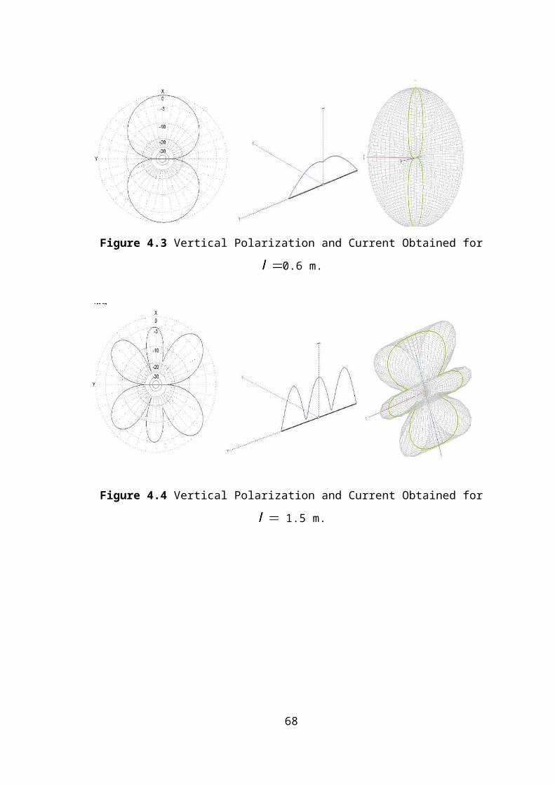
Figure 4.21 and 4.22 present the simulation results that are obtained for = 3 and = 7

elements for Yagi-Uda Antenna. These Figures illustrates: (a) is the structure of the

antenna showing the current distribution on the dipoles, (b) is the -plane radiation

pattern of the antenna (vertical polarization), (c) is the 3-D of the -plane radiation

pattern, and (d) is the horizontal polarization. The gain and input impedance for =3

and =7 elements are presented in Table 4.10.

Table 4.10 The Obtained Gain and Input Impedance for Elements = 3 and =7.

( (Ω)

3 9.1 24.16+j36.93

7 10.45 43.839+j38.43

From Table 4.10, as the number of elements increases the gain and the value of the

input impedance increase.

68

(a) (b)

(c) (d)

Figure 4.21 Simulated Results for Vertical Polarization, Horizontal Polarization,

Current Distribution and 3D of Radiation Pattern Obtained for =3 Elements Using

Yagi-Uda Antenna.

69

(a) (b)

(c) (d)

Figure 4.22 Simulated Results for Vertical Polarization, Horizontal Polarization,

Current Distribution and 3D of Radiation Pattern Obtained for =7 Elements Using

Yagi-Uda Antenna.

70

4.6 Analysis of Yagi-Uda Antenna

The Yagi-Uda antenna can be analyzed according to the theoretical part and the results

obtained from the antenna software as follows.

4.6.1 Theoretical Analysis

The second dipole in the Yagi-Uda array is the only driven element with applied

input/output source feed, all the others interact by mutual coupling since they receive

and reradiate EM energy; they act as parasitic elements by induced current. It is

assumed that an antenna is a passive reciprocal device, and then maybe used either for

transmission or for reception of the electromagnetic energy. The impedance of an

element is the value of pure resistance at the feed point plus any reactance (capacitive or

inductive) that is present at that feed point.

Maximum energy transfer of RF at the design frequency occurs when the

impedance of the feed point is equal to the impedance of the feed line. In most antenna

designs, the feed line impedance will be 50 Ω, but usually the feed point impedance of

the Yagi-Uda is rarely 50 Ω. In most cases it can vary from approximately 40 Ω to

around 10 Ω, depending upon the number of elements, their spacing and the antenna's

pattern bandwidth. If the feed line impedance does not equal the feed point impedance,

the driven element cannot transfer the RF energy effectively from the transmitter, thus

reflecting it back to the feed line resulting in a Standing Wave Ratio. Because of this,

impedance matching devices are highly recommended for getting the best antenna

performance.

The impedance bandwidth of the driven element is the range of frequencies above

and below the center design frequency of the antenna that the driven elements feed point

will accept maximum power (RF), from the feedline.

The radiation pattern of antenna plot plays a major role in the overall performance

of the Yagi-Uda antenna. The directional gain, front-to-back ratio, beam width, and

unwanted (or wanted) side lobes combine to form the overall radiation pattern [27]. The

radiation pattern bandwidth is the range of frequencies above and below the design

frequency in which the pattern remains consistent. The amount of variation from the

antenna's design specification goals that can be tolerated is subjective, and limits put

71

into the design are mainly a matter of choice of the designer. Equal spaced, equal length

directors may give higher gain at a particular frequency, but the bandwidth is narrower

and larger side lobe levels are created. Wide spacing will increase the bandwidth, but

the side lobes become large. More directors within a given boom length won't increase

the gain by any great amount, but will give a better control of the antenna's pattern over

a wider range of frequencies in the band of design.

With highest forward gain design, the main lobe becomes narrower in both the

elevation and azimuth planes, and a back lobe is always present. When the back lobe, is

designed, the pattern gets wider and the forward gain goes down. In some cases, the side

lobes become quite large. The Gain alone should not be the primary choice in Yagi-Uda

array design, since F/B ratio and impedance bandwidth value are highly influenced.

Yagi-Uda design needs compromises in Gain, Front/Side-lobes ratio for both E and H

plane and the Impedance bandwidth to avoid impractical or unusable antenna.

Generally, a loss gain of about 0.7 dB and more has required to getting better overall

and stable antenna performance. It is very hard to get high F/B ratio, i.e. a low noise

antenna, for 50 or 75 Ω intrinsic impedance at the feed point when antenna project

require maximal gain. Lowering the radiator impedance helps to get better F/B ratio. A

nice compromise could result when the intrinsic antenna impedance is around 30 +/- 10

Ω.

A wide impedance bandwidth results in good design by adding one director near

the driven element to magnify the bandwidth. The skin loss and the Joule effect in the

elements can dissipate a lot of energy at lower impedance values, resulting in an

effective lowers gain than what would expected by the theoretical calculus.

4.6.2 Analysis of Yagi-Uda Antenna by Using Software

The results of the simulations carried out, are presented in graphical form and tables.

They are intended to provide a simple means of designing a Yagi-Uda antenna of

practical dimensions with maximum gain for the configuration under consideration. The

purpose of these simulations was to determine the following:

1. Effect of reflector spacing on the gain of a dipole antenna.

2. Effect of different equal length directors, their spacing and number of directors.

72

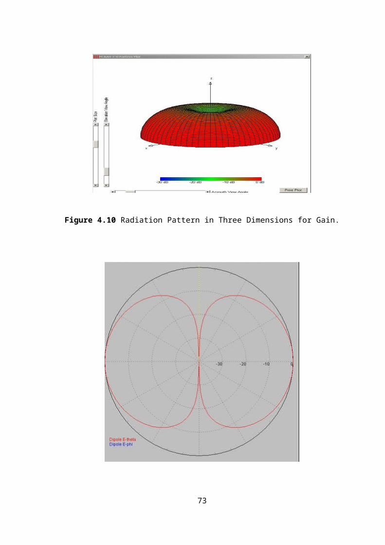
3. Effect of different spacing of directors.

From Figures 4.16 to 4.18, Yagi-Uda has been simulated using PCAAD and by

changing the numbers of directors starting from = 3, 4,5,6,7, respectively, leads in

change of the gain and impedance. From Table 4.7, the more directors the more focused

the gain is in the direction of the directors which lead to incensement in the amount of

gain and decrease the bandwidth of the radiation patterns. All real antennas have both

sidelobes and backlobes; these lobes represent wasted power transmitted in the wrong

direction during transmission and interference opportunities while receiving. In most of

the cases the driven element is a folded dipole.

This serves two purposes. Firstly, the input impedance of the driver is increased.

This is desirable because the input resistance values as shown in the Table 4.7, which

are computed for an ordinary resonant half wave dipole feed, are relatively low and not

well matched to common transmission lines, secondly the electrical performance of the

antenna will remain stable over a wider band width when a folded dipole feed is used.

The goal of the antenna designer is to increase the main lobe while decreasing the side

lobes and back lobes, from figures side lobes are varying but they have no effect on

performance due to folded dipole. From Figure 4.19 and Table 4.8, it is obtained that

when the same numbers of elements are used and the spaces are changed this will affect

on the characters of the antenna as the spaces increases between the directors, the gain

increases. Due to that Yagi-Uda antenna gain is highly sensitive and depends upon

numerous parameters and therefore it is difficult to optimize.

4.7 Implementation of Yagi-Uda Antenna

There are three main parameters used to characterize the performance of a particular

Yagi-Uda antenna which are gain, pattern radiation and input impedance. The

implementation of an antenna will be done according to the range of frequencies that is

used by channels from Bayrak Radio and Television Corporation (BRTK) [30]. Ranges

of frequencies that the channels of BRT and TRT are given by Table 4.10.

73

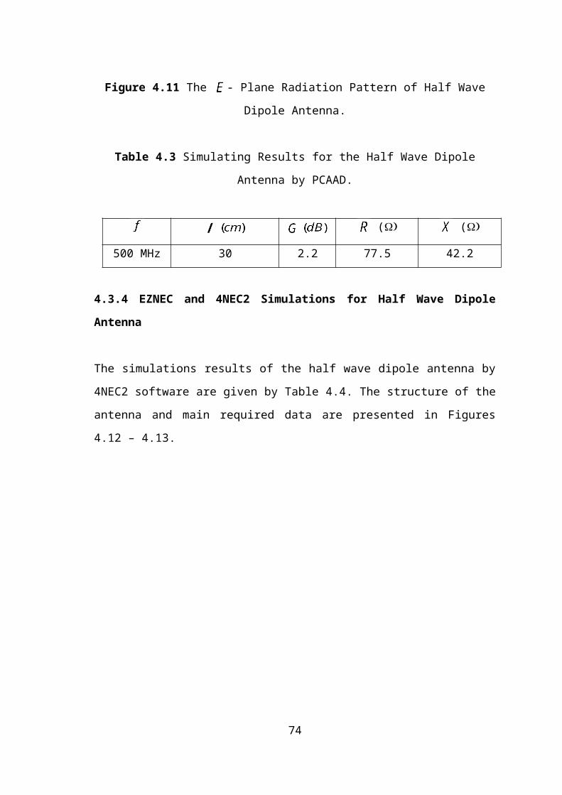
Table 4.11 Commonly Used Frequencies in RRTK TV [30].

Region 1 (EAST) Location: Sinandağı

Channel TV. Channel

VHF 08 TRT1

UHF 21 BRT1

UHF 50 BRT2

Region 2 (WEST) Location: Selvilitepe

VHF 11 TRT1

UHF 41 TRT2

UHF 44 BRT1

UHF 33 BRT2

For instance channel TRT1 is broadcasting from Selvilitepe. From Table 4.11, TRT1 is

considering as channel 11. In order to know in which frequency the channel 11 operates

the range of the frequency should be known. Appendix C presents the ranges of

frequencies for the channels which are given by American Radio Relay League (the US

national organization of Amateur Radio operators) [31]. As TRT1 operates at channel

11, the frequency range is 199.25 and BRT2 operates at channel 33, the frequency

range is 585.25 . So to receive the signals which are broadcasting from Selvilitepe,

the average will be taken from lower frequency and upper frequency which gives 392.25

. Basics of Stutzman will be used from Table 2.2 in order to simulate the desired

antenna.

In order to find the parameters of the antenna, the following steps are calculated for

.

Element Number,

Radius of each element,

Reflector length,

Feeder length,

Directors length,

74

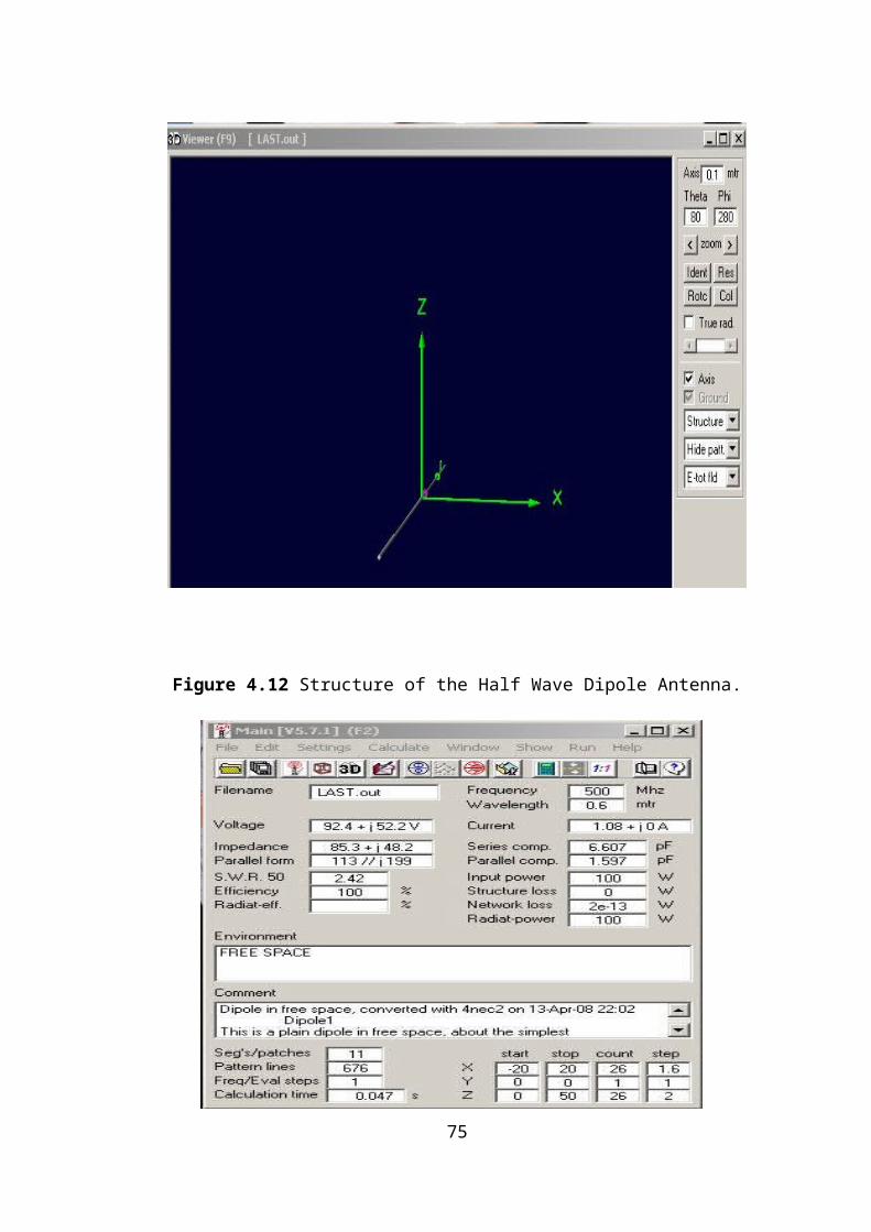
Space between directors,

In accordance of the above given data, Yagi-Uda Antenna was simulated using EZNEC

and 4NEC2X, to obtain the following output results.

(a)

75

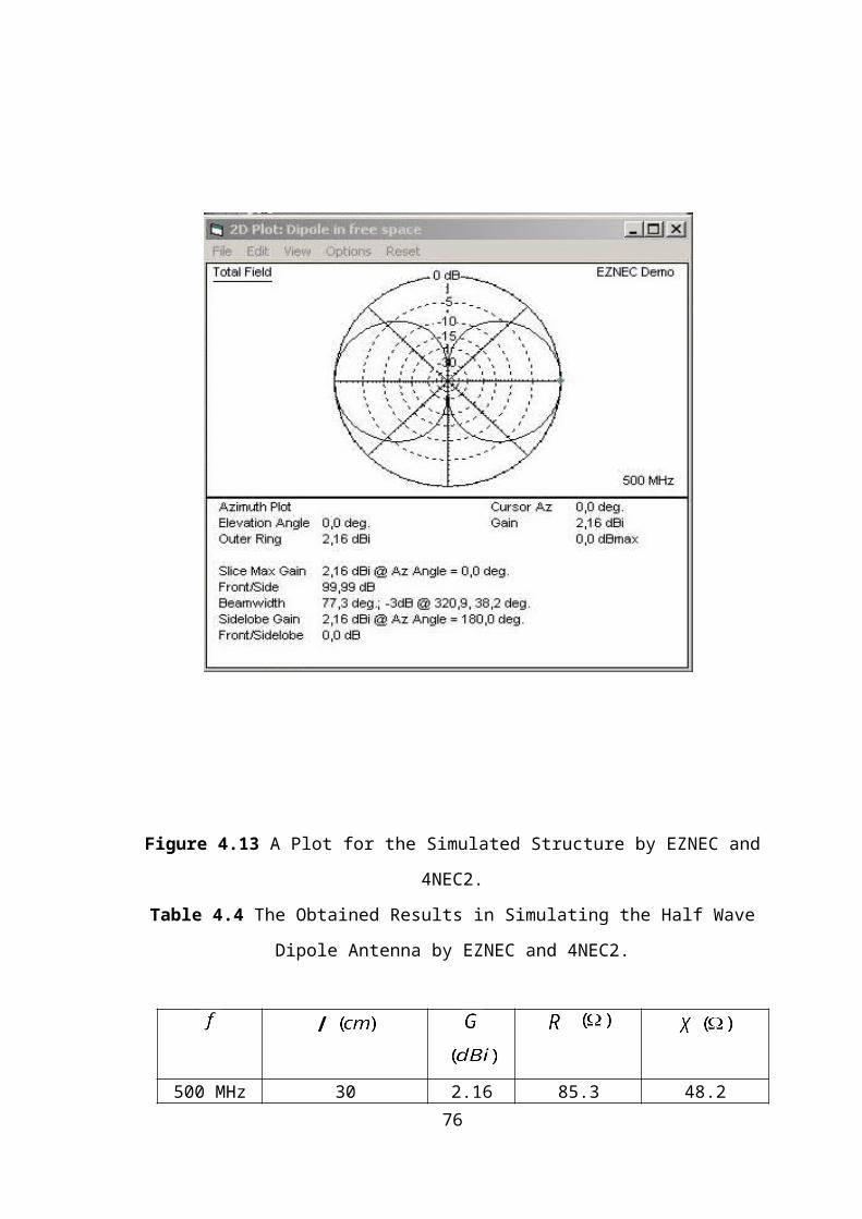
(b) (c)

(d)

76

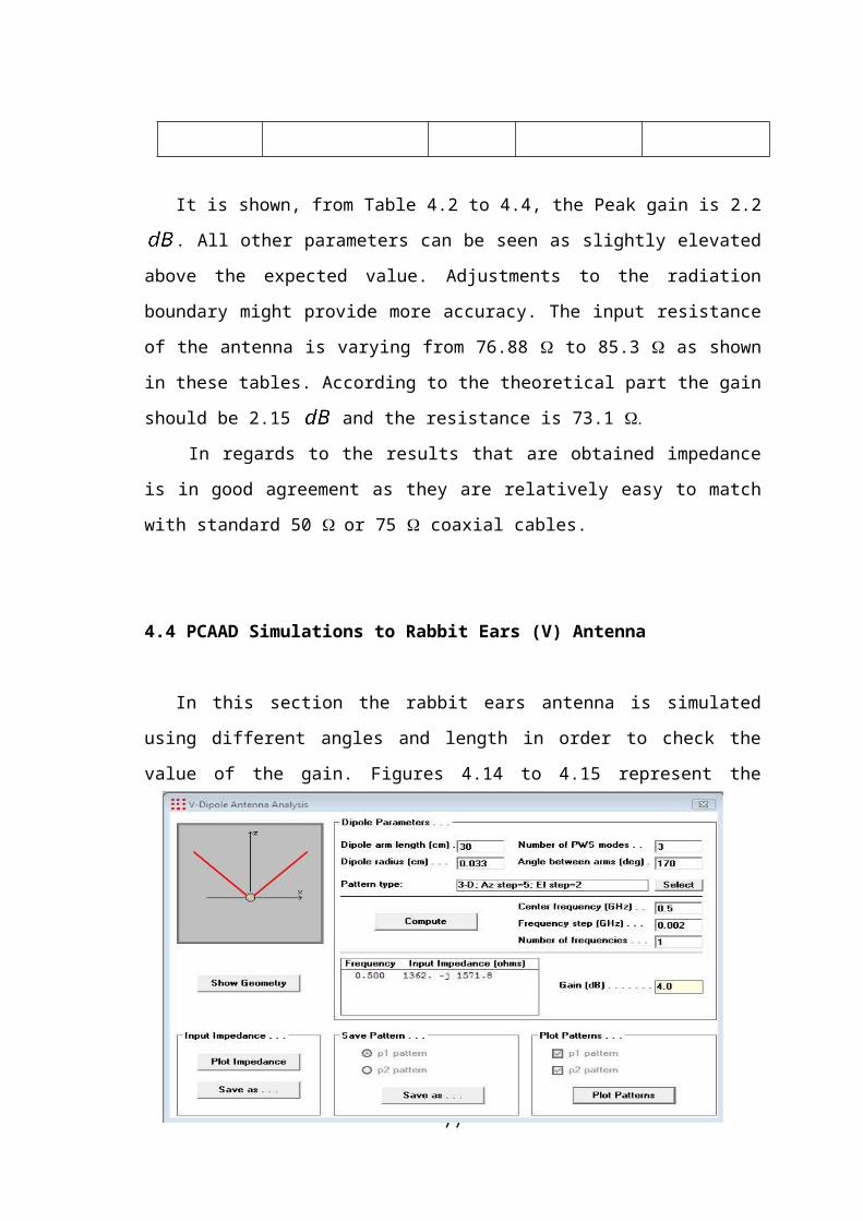
(e)

Figure 4.23 Simulated Results for Vertical Polarization, Horizontal Polarization,

Current Distribution and 3D of Radiation Pattern Obtained for =5 Elements for Yagi-

Uda Antenna Designed.

From Figure 4.23 (a) presents the numerical output results of the simulated data, (b)

presets the vertical pattern, (c) presents the horizontal pattern, (d) the structure of the

antenna and the distribution of the current on the elements, and (e) presents the

horizontal radiation in respect of gain where the amount of the gain can be obtained

from the figure, the mechanical and environmental part was not considered in the

design.

The implementation of the Yagi-Uda antenna was successfully simulated and good

results were obtained. Table 4.12 presents the main parameters of the implemented

antenna.

77

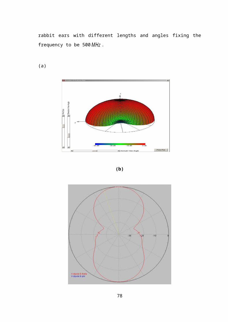
Table 4.12 Gain, Input Impedance and Efficiency for = 5, 7 Elements Obtained for

this Work.

( (Ω) %

5 9.17 8+j12.4 96.64

7 11.19 27.5+j1.35 91.64

In this design two models were obtained, from Table 4.11 the gain with 7 elements

have higher than 5 elements but after the graphs are obtained the efficiency in 7

elements is less than 5 elements and the side lobs are more in 7 elements, due to that

when an antenna is designed many parameters should be considered, therefore 5

element was considered. Maximum energy transfer of RF at the design frequency

occurs when the impedance of the feed point is equal to the impedance of the feed line,

the feed line impedance is 50 Ω, and feed point impedance of the Yagi-Uda is rarely 8

Ω, not to forget that this result should be added with a balun in order to balance the

system to get good performance.

4.8 Summary

In this chapter, different types of antenna using various software were used to analyze

the different types of dipoles such as half wave dipole antenna and rabbit ears. As an

application for dipole antenna Yagi-Uda was considered as one of the main types of

dipoles. In half wave dipole antenna the relationship between the gain of a dipole and its

height above a perfectly conducting ground plane, the dependence of gain and feed

point impedance on the length of a dipole was simulated and analyzed.

In case of rabbit ears the effect of changing the length and angles of the antenna to the

gain was discussed. Yagi-Uda was simulated using different elements with same spaces

of dipoles and different spaces in order to check its effeteness on the performance of the

antenna. An implemented antenna was designed in order to operate in a range of

frequency in Turkish Republic of Northern Cyprus (TRNC). The obtained simulated

results are found to be in good agreement with the theoretical one.

78

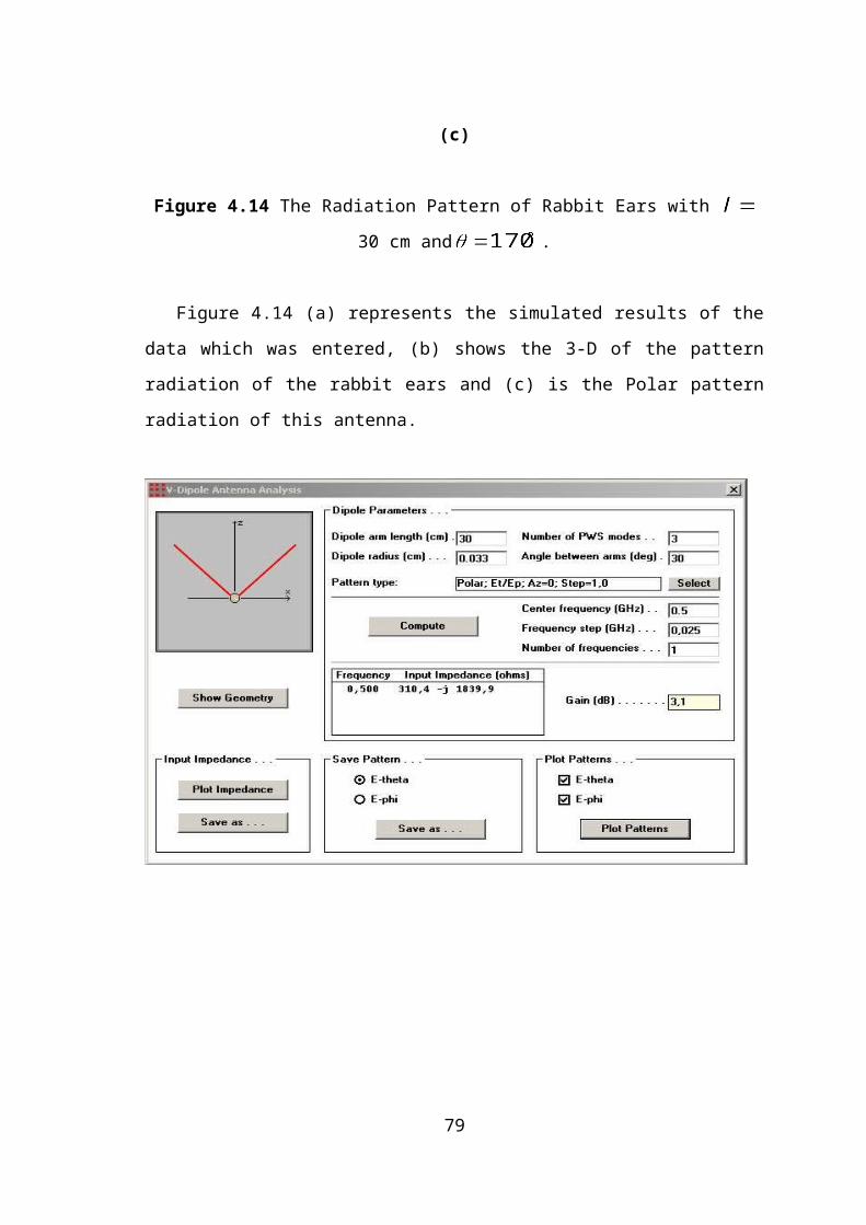
CONCLUSION

This work covered basic antenna definitions and explained terms frequently

encountered in examining antenna parameters and its characteristics. Gain, input

impedance beam width definitions and pattern parameters such as front-to-back ratio

and side lobe levels were discussed. A short survey of three important numerical

simulation methods used by the EM software which are MoM, FEM and FTDT were

explained. All the software that have been utilized in this work were using MoM

method. The -plane patterns for six different dipole lengths calculated and drawn in

terms of wavelength are simulated using the MATLAB. The -plane radiation pattern

results shown and compared with the theoretical part. The radiation pattern for = ,

, , , and were plotted. From the Figure 4.1 that was plot, it is seen that as

increase the length of the dipole increase, the lobes will increase. This would affect on

the performance of the antenna. Table 4.1 presented the numerical calculations for the

different lengths of dipole antenna

MMANA software was simulated to investigate the dependence of grain and feed

point impedance on the length of a dipole in free space. According to the results, dipole

gain increases when the length of the dipole increases, the resonance occurs at slightly

less than one-half wavelength and radiation resistance is about 75 Ω. The half-wave

dipole has a single current peak, while the 1.5 dipole has three current peaks, each

acting as a source of radiation, so that interference can be expected, dipoles longer than

one wavelength exhibited unwanted side lobes, while shorter ones are not. Due to that

the half wave dipoles are popular because they are relatively easy to match to standard

50 or 75 coaxial cables as they do not contain side lobes. Figure 4.2 to 4.8 presents

the results which were obtained.

Half wave dipole antennas were simulated by PCAAD and EZNEC to calculate the

gain and the input impedance. The input resistance of the antenna was varying from

76.88 to 85.3 and gain was varying from 2.16 to 2.2 as shown in Table 4.3

to 4.4 and Figure 4.9 to 4.13. According to the theoretical point of view the gain should

be 2.15 and the resistance is 73.1

The Rabbit ears antenna was simulated by using different angles and length. The

results showed that adjusting the length of each leg would make the antenna resonant on

different frequencies. Adjusting the angle between the two "ears" is found to affect the 79

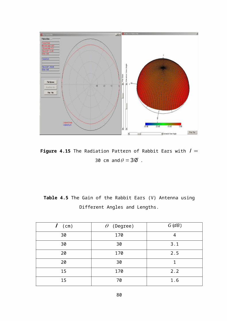
radiation pattern. Making a smaller angle makes the antenna behaving more like an

isotropic radiator, i.e., it receives signals all around with almost no attenuation. Once the

angle is increased, the pattern becomes a straight dipole, having deep nulls at each end

as in Figures 4.14 to 4.15 and Table 4.5.

Having investigated the dipole antenna and rabbit ears, one would state the

following as the frequency ( ) increases wavelength decreases, Gain is inversely

proportional to wavelength, so as frequency increases gain also increases.

Furthermore, the gain is directly proportional to Area of the aperture, so as the area

of the antenna increases gain also increases. Noting that gain is inversely proportional to

beam width. As side lobe level increases, the signals will be spitted in the unwanted

direction and signal strength at the required direction will be less.

A Yagi-Uda Antenna, commonly known simply as a Yagi antenna or Yagi, is a

directional antenna system consisting of an array of a dipole and additional closely

coupled parasitic elements (usually a reflector and one or more directors). PCAAD,

EZNEC, MMANA were used to simulate the Yagi-Uda antenna. The aim of such

simulations is to determine the effect of reflector spacing, on the gain of a dipole

antenna, the effect of different equal length directors on the gain of the antenna, their

spacing and number of directors and the effect of different spacing of directors to the

gain. Yagi-Uda has been simulated by changing the numbers of directors starting from

elements = 3, 4, 5, 6, 7 respectively, which leads in change of the gain and

impedance. The more directors, the more focused the gain is in the direction of the

directors which lead to incensement in the amount of gain and decrease the bandwidth

of the radiation patterns which are presented in Figures 4.16 to 4.18 .

Same numbers of elements were used and the spaces were changed. This change

has affected on the characters of the antenna, the spaces between the directors increase,

the gain also increases which is presented in Table 4.8 and Figure 4.19.

Results shows that when element = 6 is a good antenna because it has high gain

as well as input impedance which is matching to the standard 50 of the coaxial

cables. Yagi-Uda antenna gain is highly sensitive and depends upon numerous

parameters and therefore it is difficult to optimize.

If directional antennas, or beam antennas over dipole are compared with vertical

antennas, it is seen that a beam antenna concentrates mostly of its transmitted signal in

one compass direction. The Directivity or gain is provided in the direction the antenna is

80

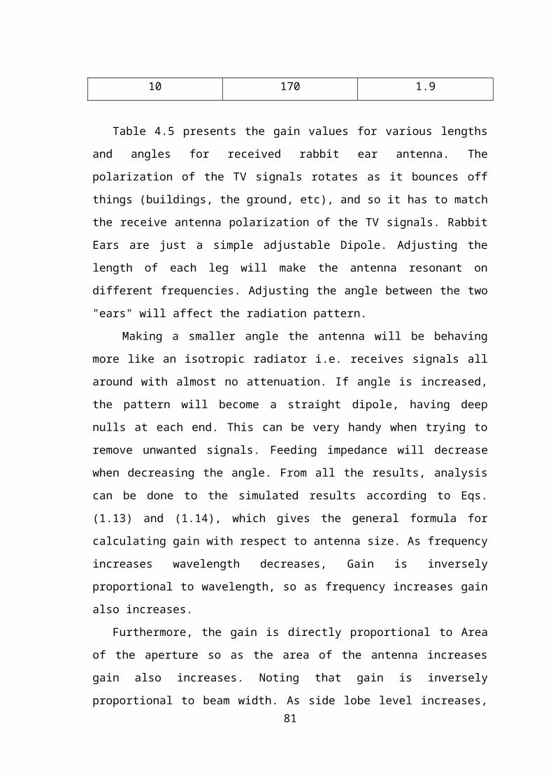
pointed. This makes the signal sound stronger to other operators and vice versa, when

compared with non-directional antennas. Secondly, the reduction in the strength of

signals coming from directions other than where the point is. By reducing the

interference from stations in other directions the operating enjoyment in the desired

direction can be increased.

On the other hand, an implementation of Yagi-Uda antenna was designed and simulated

in accordance with the broadcasting channels of Bayrak Radyo ve Televizyon Kurumu

(BRTK) in Turkish Republic of Northern Cyprus (TRNC).

The mechanical and environment side were not considered in the simulations, but

the main parameters to be used in calculating the gain, input impedance and efficiency

were given. Channels that are broadcasting from Selvilitepe were the main subject of

study, thus, the utilized frequency was calculated according to the range which this

channel operates. The following Figures: the numerical output results of the simulated

data, the horizontal pattern, the vertical pattern, the structure of the antenna and the

distribution of the current on the elements, the 3D of the vertical and horizontal

radiation pattern and the horizontal radiation in respect of gain where the amount of the

gain can be obtained from the Figure 4.24. From numerical results, the parameters were

= 5, = 9.17 , = 8+j12.4 Ω, = 96.64 % which are considered better result

than N=7.

These results are presented in Table 4.12. Therefore, from results and graphs,

according to the theoretical point of view this type of antenna has a good performance.

Further, in this work dipole antennas such as half wave dipole antenna, rabbit ears

antenna and Yagi-Uda antenna were constructed and analyzed.

Finally, various types of antennas would be also simulated such as horn antenna,

helical antenna or possibly the more developed antennas such as smart antennas.

Computer software were used to design the implemented antenna, this type of

antenna can be done in real life, so practical and experimental methods can be used for

these types of antenna, or other types.

81

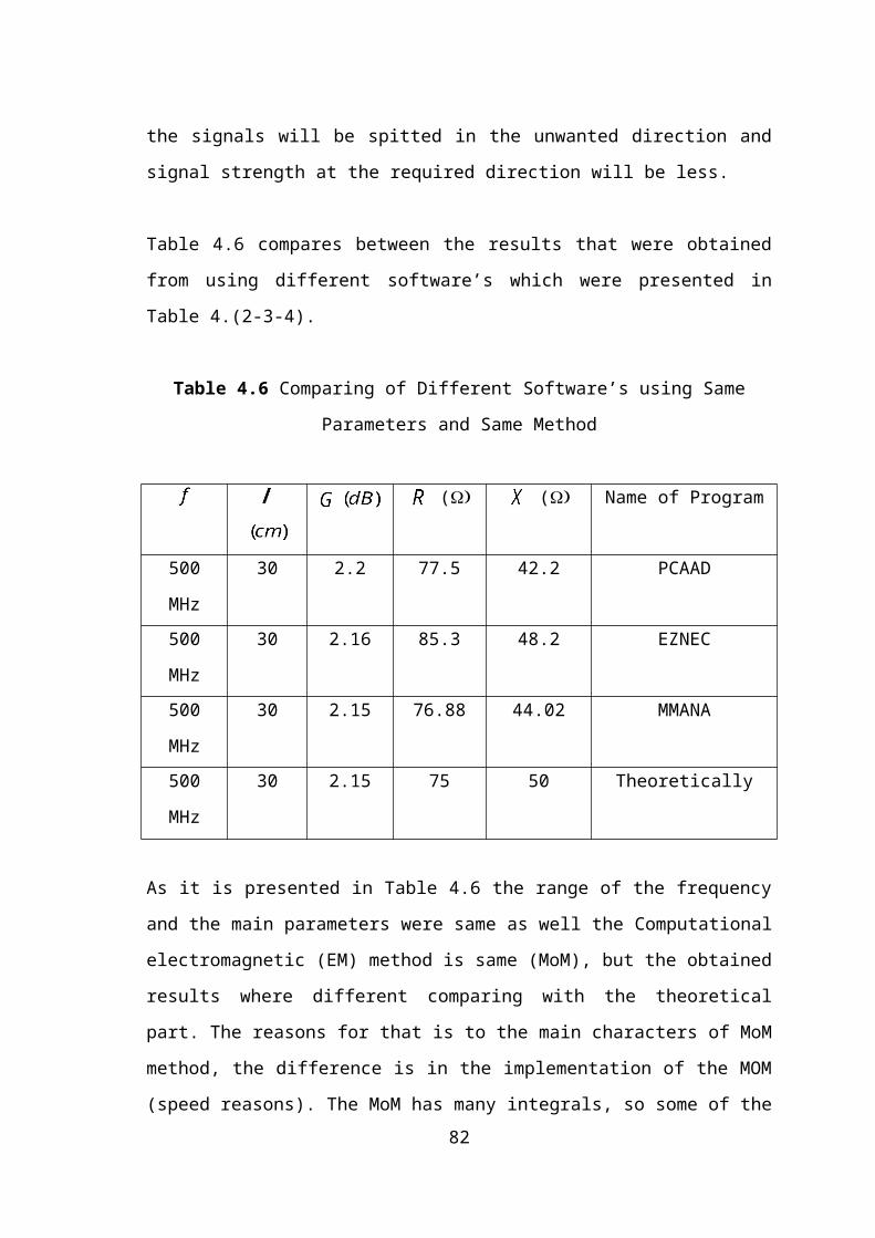
REFERENCE

[1] Stutzman, W. L.; Thiele, G. A. (1998). Antenna Theory and Design, John Wiley

& Sons, Inc.

[2] US Marine Corps. (1991). Field Antenna Handbook.

[3] Balanis, C. A. (1997). Antenna Theory Analysis and Design, John Wiley & Sons,

Inc.

[4] Makarov, S. N. (2002). Antenna and EM Modeling with MATLAB, John Wiley

& Sons, Inc.

[5] Ulaby, F.T. (1999). Fundamentals of Applied Electromagnetics, Prentice Hall.

[6] Wireless Networking. (2008). Antennas and Transmission Lines, front to back

ratio. From the World Wide Web: http://www.vias.org wirelessnetw/wndw

_06_05_08.html.

[7] Yaghjian, A.D.; Best, S.R. Impedance, bandwidth, and Q of antennas, IEEE

Transaction on Antennas and Propagation, pp.1298-1324, April 2005.

[8] Wikipedia. (2008). Dipole Antenna. From the World Wide web:

http://en.wikipedia.org /wiki/ Dipole_antenna.

[9] Cheng, D. K. (1993). Fundamentals of Engineering Electromagnetic, Addison

Wesley Publishing Company, Inc.

[10] Yong, S.K.; Thompson, J.S. The Effect of Antenna Parameters on the

Performance Analysis of Different Antenna array Architectures, IEEE

Conference on Personal Mobile, Communications, 5th European, pp. 5-10, 2003

[11] Lule, E.; Babij, T.; Siwiak, K. Analysis using FDTD of Ultra-Wideband Dipole

Antennas. IEEE International Symposium on Antennas and Propagation

Society, Volume 1, pp. 838-841, 2003

[12] Albreem, H. (2003). Implementation and Measurements on the Half-Wave

Dipole Antenna, M.S.c. Thesis, Nicosia: Near East University Library.

[13]

[14]

Attar, H. (1999). Design and Investigation of the Antenna Measurement systems,

M.S.c. Thesis, Nicosia: Near East University Library.

Kim, K.; Yang, S. Efficiency of Resistive Vee Dipole Antenna IEEE, on

Electronics Letters, Oct 2007.

82

[15] Meie Chen; Junhong Wang. Study on V-Shaped Dipole Antenna Array for Pulse

Radiation, IEEE International Symposium on Microwave, Antenna, Propagation

and EMC Technologies for Wireless Communications, pp. 723-726, Aug. 2007

[16] Wikipedia. (2008). Yagi-Uda Antenna. From the World Wide Web:

http://en.wikipedia. org/Wiki/ Yagi_antenna.

[17] Lei Juan; Fu Guang; Yang Lin; Fu Demin. Optimization and Application of the

Yagi-Uda Antenna for Meteor Burst Communication, IEEE International on

Symposium Microwave, Antenna, Propagation and EMC Technologies for

Wireless Communications ,pp 669-672, Aug. 2007

[18] Xue, D. (2002). Yagi Uda Antenna, The Institute for Computational Engineering

and Sciences. From the World Wide Web:

http://users.ices.utexas.edu/~cynthia/paper/yagi.pdf

[19] El-khouly, Essam A. Ghali, Hani A. High Gain Fractal-Based Yagi Antenna,

IEEE Conference on Antennas and Propagation, pp. 405-406, March 2008

[20] Jones, E.A.; Joines, W.T. Design of Yagi-Uda Antennas using Genetic

Algorithms. IEEE Transaction on Antennas and Propagation, pp.1386-1392, Sep

1997.

[21] Jonathan.; Imberi, S. (2008). Pointing Beam Antennas. From the World Wide

Web:http://ham-shack.com/beam.html.

[22] Carr, Joseph. J. (2001). Practical Antenna Handbook. McGraw-Hill Companies,

Inc.

[23] Introduction to Computational EM, Embedded Internet Systems Laboratory,

From the World Wide Web:

http://www.er.sm.luth.se/er/course.nsf/0/d3e865fd88081289c1256e4d002bdbb7/$

FILE/Lecture13.pdf.

[24] Personal Computer Aided Antenna Design, From the World Wide Web:

http://www.antennadesignassociates.com/pcaad5.htm.

[25] Numerical Electromagnetic Computation, From the World Wide Web:

http://www.si-list.net/swindex.html.

[26] EZNEC, From the World Wide Web: http://www.eznec.com.

[27] Makoto Mori Antenna Analysis, From the World Wide Web:

http://mmhamsoft.amateur-radio.ca/.

83

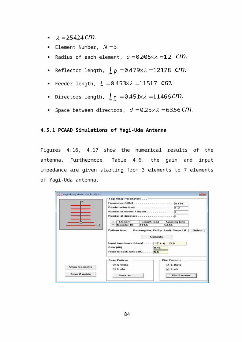
[28] Mittra, R. Challenges in Antenna Designs and Some Novel Techniques for

Meeting Them, IEEE Conference on Antennas and Propagation, pp 1-4, April

2007.

[29] Agilent, 3D Full-wave Electromagnetic Field Simulation, High Frequency

Structural Simulator, http://www.ansoft.com/products/hf/hfss/.

[30] Bayrak Radio and Television Corporation, Our Frequencies. From the World

Wide Web: http://www.brtk.cc/index.php/lang/en/cat/89.

[31] American Radio Relay League, TV Channel, CATV and FM Broadcast

Frequencies. From the World Wide Web: http://www.arrl.org/tis/info/catv-

ch.html.

84

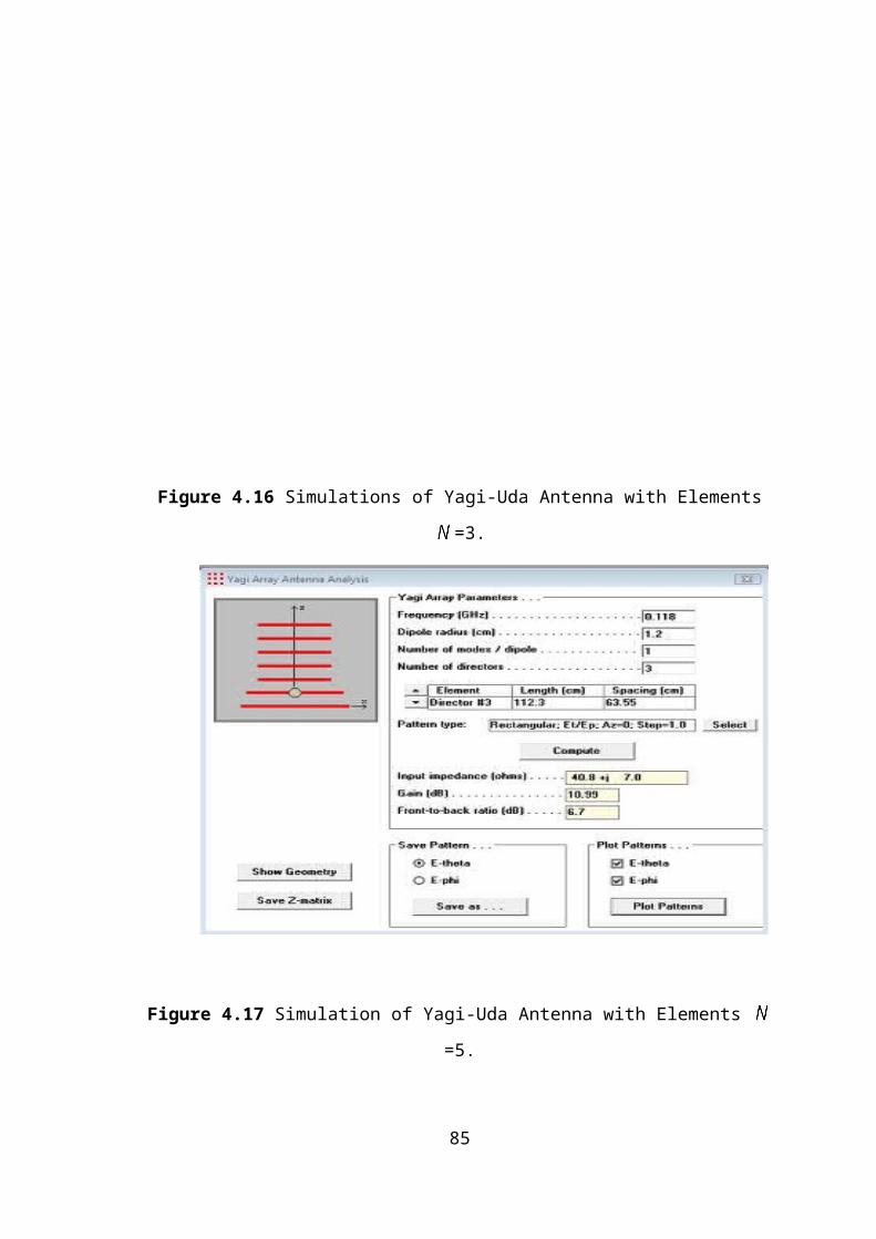
APPENDIX A

MAXWELL'S EQUATIONS [23]

85

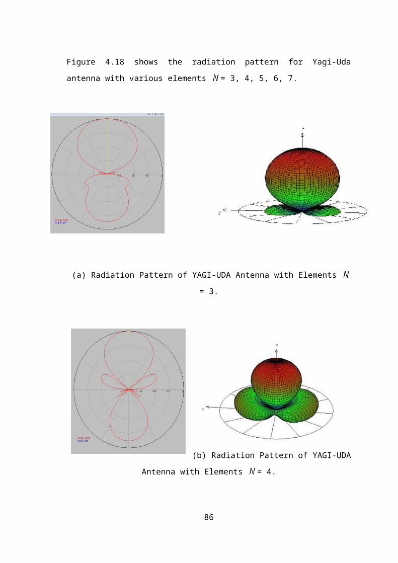
APPENDIX B

MATLAB PROGRAM TO SIMULATE Eq. (2.8)

lamda=input('enter the value of wave length= ');

L=input('enter your dipole length L= ');

ratio=L/lamda;

B=(2*pi/lamda);

theta= pi/100:pi/100:2*pi;

if ratio<= 0.1 % it should check if it is Short Dipole or not

E=sin(theta);

En=abs(E);

subplot(2,3,1)

polar(theta,En) %This plot polar pattern in plane which dipole appear as line

else %check if not short dipole

f1=cos(B*L/2.*cos(theta));

f2=cos(B*L/2);

f3=sin(theta);

E=(f1-f2)./f3;

En=abs(E);

subplot(2,2,2)

polar(theta,En) % Plot polar pattern in plane

end

86

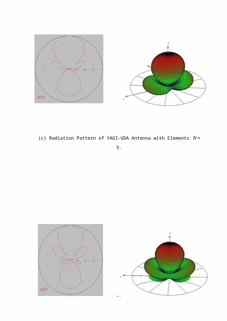
APPENDIX C

CHANNELS AND FREQUENCIES [31]

TV Channe

l

Frequenc

y

Range Note

AIR 2 55.25 VHF-LO

AIR 3 61.25 VHF-LO

AIR 4 67.25 VHF-LO

AIR 5 77.25 VHF-LO

AIR 6 83.25 VHF-LO

AIR 7 175.25 VHF-HI

AIR 8 181.25 VHF-HI

AIR 9 187.25 VHF-HI

AIR 10 193.25 VHF-HI

AIR 11 199.25 VHF-HI

AIR 12 205.25 VHF-HI

AIR 13 211.25 VHF-HI

AIR 14 471.25 UHF

AIR 15 477.25 UHF

AIR 16 483.25 UHF

AIR 17 489.25 UHF

AIR 18 495.25 UHF

87

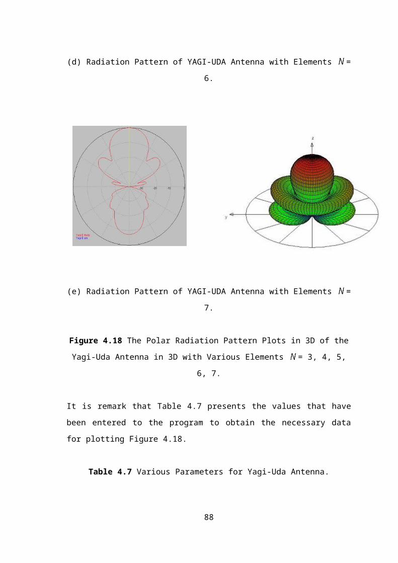
AIR 19 501.25 UHF

AIR 20 507.25 UHF

AIR 21 513.25 UHF

AIR 22 519.25 UHF

AIR 23 525.25 UHF

AIR 24 531.25 UHF

AIR 25 537.25 UHF

AIR 26 543.25 UHF

AIR 27 549.25 UHF

AIR 28 555.25 UHF

AIR 29 561.25 UHF

AIR 30 567.25 UHF

AIR 31 573.25 UHF

AIR 32 579.25 UHF

AIR 33 585.25 UHF

AIR 34 591.25 UHF

AIR 35 597.25 UHF

AIR 36 603.25 UHF

AIR 37 609.25 UHF

AIR 38 615.25 UHF

AIR 39 621.25 UHF

88

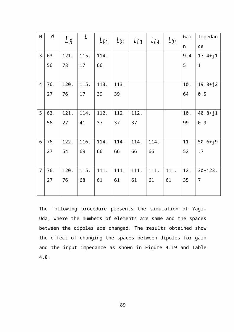
AIR 40 627.25 UHF

AIR 41 633.25 UHF

AIR 42 639.25 UHF

AIR 43 645.25 UHF

AIR 44 651.25 UHF

AIR 45 657.25 UHF

AIR 46 663.25 UHF

AIR 47 669.25 UHF

AIR 48 675.25 UHF

AIR 49 681.25 UHF

AIR 50 687.25 UHF

AIR 51 693.25 UHF

AIR 52 699.25 UHF

AIR 53 705.25 UHF

AIR 54 711.25 UHF

AIR 55 717.25 UHF

AIR 56 723.25 UHF

AIR 57 729.25 UHF

AIR 58 735.25 UHF

AIR 59 741.25 UHF

AIR 60 747.25 UHF

89

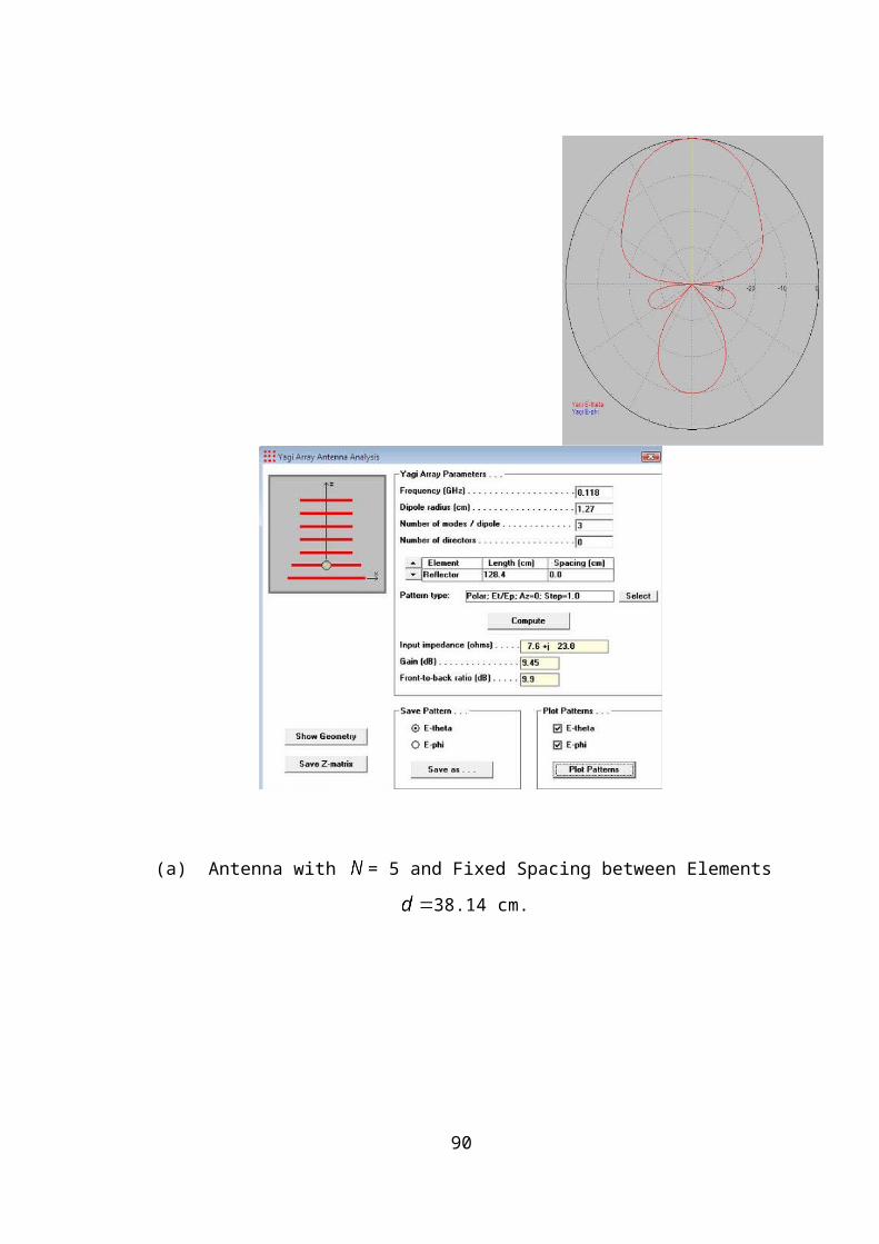
AIR 61 753.25 UHF

AIR 62 759.25 UHF

AIR 63 765.25 UHF

AIR 64 771.25 UHF

AIR 65 777.25 UHF

AIR 66 783.25 UHF

AIR 67 789.25 UHF

AIR 68 795.25 UHF

AIR 69 801.25 UHF

AIR 70 807.25 UHF (no longer assigned to

TV)

AIR 71 813.25 UHF (no longer assigned to

TV)

AIR 72 819.25 UHF (no longer assigned to

TV)

AIR 73 825.25 UHF (no longer assigned to

TV)

AIR 74 831.25 UHF (no longer assigned to

TV)

AIR 75 837.25 UHF (no longer assigned to

TV)

AIR 76 843.25 UHF (no longer assigned to

TV)

AIR 77 849.25 UHF (no longer assigned to

90

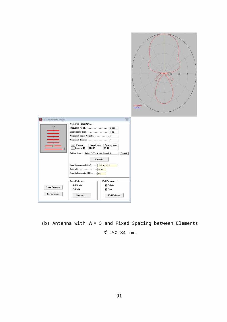
TV)

AIR 78 855.25 UHF (no longer assigned to

TV)

AIR 79 861.25 UHF (no longer assigned to

TV)

AIR 80 867.25 UHF (no longer assigned to

TV)

AIR 81 873.25 UHF (no longer assigned to

TV)

AIR 82 879.25 UHF (no longer assigned to

TV)

AIR 83 885.25 UHF (no longer assigned to

TV

91