Embed Size (px)
Citation preview
Bismi ALLAH Arrahman Arraheem
Class Notes of Principles of Macroeconomics Econ.102 BY
Dr. Usamah Ahmed UthmanAssociate Professor of Economics
Department of Finance & EconomicsKing Fahd University of Petroleum& Minerals
Dhahran 31261Saudi Arabia
http://faculty.kfupm.edu.sa/finec/osama/
1
KING FAHD UNIVERSITY OF PETROLEUM & MINERALSCollege of Industrial Management
Department of Finance & EconomicsEcon 102 : Principles of Economics II (Macroeconomics)Instructor : Dr. Usamah Ahmed UthmanOffice : B24/296Web Site : http://faculty.kfupm.edu.sa/finec/osama/
Office Hours :11:45 – 12:45 PM, S,M (or by appointment)Textbook :Economics by Lipsey, et al, 12th Ed.
Course Outline
Chapter 21 : What Macroeconomics Is All About?Chapter 22 : The Measurement of National IncomeChapter 23 : National Income Determination – Part 1Chapter 24 : National Income Determination – Part 2
Applications to the Multiplier Theory Chapter 25 : Output and Prices in the Short RunChapter 26 : Output and Prices in the Long RunChapter 27 : The Nature of Money and Monetary InstitutionsChapter 28 : Money, Output, and PricesChapter 29 : Monetary PolicyChapter 30 : InflationChapter 31 : UnemploymentChapter 32 : Government Debt and DeficitsChapter 37 : Exchange Rates and the Balance of Payments
First Exam 20%Second Exam 20%Quizzes and participation 20%Final Exam (Chapters 22,24,26,28,29,31,32,and 37) 40% Total 100%
NOTE: Professor reserves the right to change the contents and weights of course requirements.FIRST MAJOR EXAM, Wednesday, 8 Shaa'ban,1433 (27 June, 2012). Bldg.24/121, 7:00- 9:00 PMSECOND MAJOR EXAM, Tuesday, 28 Shaa'ban, 1433 (17 July, 2012)Bldg. 24/121, 7:00 – 9:00 PM
CHAPTER 21
2
INTRODUCTION TO MACROECONOMICS
Economics' two -major branches are:
Microeconomics: discusses individual economic units: the firm, the consumer, particular markets, such as the oil market, the computers mkt, the tomatoes mkt.Macroeconomics: discusses the behavior of aggregate economic Variables, such as total investment, total consumption, govt. expenditures and taxation, unemployment, inflation, economic growth….. etc.
The two branches are related, i.e. macro events affect micro areas & vice versa.
Macro issues: What does macroeconomics discusses? I) Long term economic Growth:
1) What causes economic growth? 2) How do govt. policies affect economic growth? Through: a) Monetary policy, which regulates money supply and interest rates. b) Fiscal policy, which regulates government expenditures and taxation.
II) Short term business cycles:are short term fluctuations in economic activity. To understand business cycles we must understand inflation and unemployment.
* Economic indicators: are measures of the health of the economy, such as the rate of econ. growth, unemployment, the budget deficit., the public ( govt.) debt, the inflation rate, investment , the balance of payments deficit….etc* National product and national income: as NP , NI . * This means that the more goods and services are produced, there is more income generated for people. This is because in the process of generating output, factors of production must be employed and paid for
3
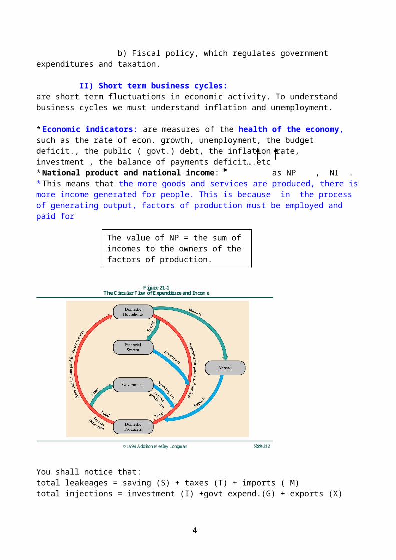
The value of NP = the sum of incomes to the owners of the factors of production.
©1999 Addison Wesley Longman Slide 21.2
Figure 21-1The Circular Flow of Expenditure and Income
You shall notice that:total leakeages = saving (S) + taxes (T) + imports ( M)total injections = investment (I) +govt expend.(G) + exports (X)
for macroeconomic equilibrium:
S + T + M = I + G + X * Nominal National income: is measured in the prices of current year, NI=PQ. It can change due to change in P, Q, or both.
* Real national income: is measured in the prices of some base year. This means we hold prices constant. When prices are held constant, changes in (real) national income reflect only changes in quantities.
* The most commonly used measure of national income is the Gross Domestic Product (GDP). It is the total value of all final goods & services produced at home.
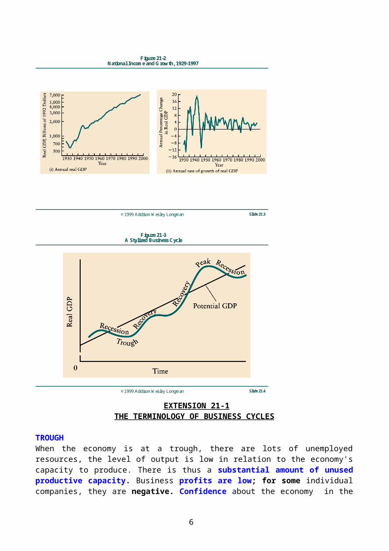
* The Business Cycle refers to the continual ups & downs in economic activity around a long term trend. This can be observed in many economic series. It is important to note that no two business cycles are exactly the same, neither in duration, nor in magnitude.
* See FIG.21-3 below. Also, see EXTENSION 21-1 below for business cycle terminology.
4
total leakages = total injection

©1999 Addison Wesley Longman Slide 21.3
Figure 21-2National Income and Growth, 1929-1997
©1999 Addison Wesley Longman Slide 21.4
Figure 21-3A Stylized Business Cycle
EXTENSION 21-1
THE TERMINOLOGY OF BUSINESS CYCLES
TROUGHWhen the economy is at a trough, there are lots of unemployed resources, the level of output is low in relation to the economy's capacity to produce. There is thus a substantial amount of unused productive capacity. Business profits are low; for some individual companies, they are negative. Confidence about the economy in the immediate future is lacking and, as a result, many firms are unwilling to risk making new investments.
5
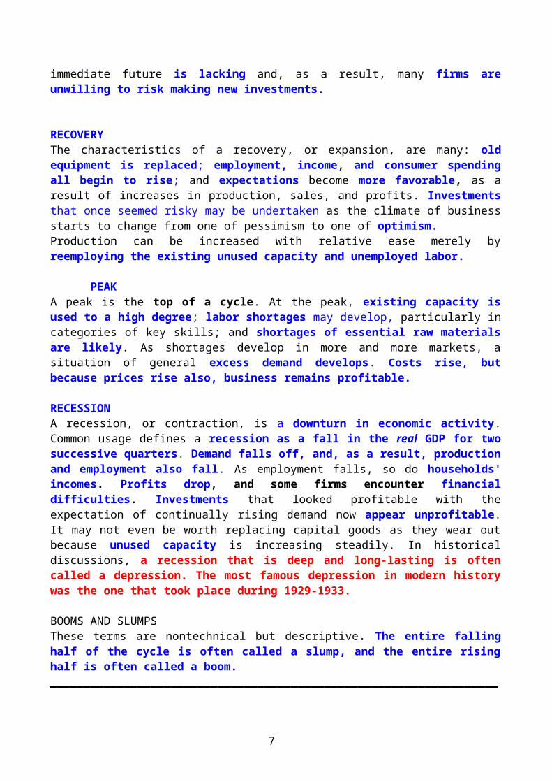
RECOVERYThe characteristics of a recovery, or expansion, are many: old equipment is replaced; employment, income, and consumer spending all begin to rise; and expectations become more favorable, as a result of increases in production, sales, and profits. Investments that once seemed risky may be undertaken as the climate of business starts to change from one of pessimism to one of optimism.
Production can be increased with relative ease merely by reemploying the existing unused capacity and unemployed labor.
PEAKA peak is the top of a cycle. At the peak, existing capacity is used to a high degree; labor shortages may develop, particularly in categories of key skills; and shortages of essential raw materials are likely. As shortages develop in more and more markets, a situation of general excess demand develops. Costs rise, but because prices rise also, business remains profitable.
RECESSIONA recession, or contraction, is a downturn in economic activity. Common usage defines a recession as a fall in the real GDP for two successive quarters. Demand falls off, and, as a result, production and employment also fall. As employment falls, so do households' incomes. Profits drop, and some firms encounter financial difficulties. Investments that looked profitable with the expectation of continually rising demand now appear unprofitable. It may not even be worth replacing capital goods as they wear out because unused capacity is increasing steadily. In historical discussions, a recession that is deep and long-lasting is often called a depression. The most famous depression in modern history was the one that took place during 1929-1933.
BOOMS AND SLUMPSThese terms are nontechnical but descriptive. The entire falling half of the cycle is often called a slump, and the entire rising half is often called a boom.___________________________________________________________________
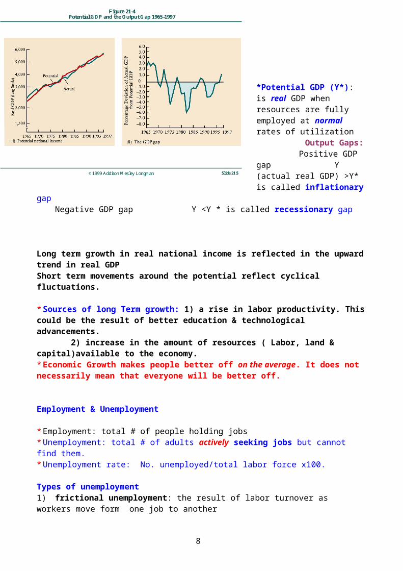
*Potential GDP (Y*): is real GDP when resources are fully employed at normal rates of utilization Output Gaps:
Positive GDP gap Y (actual real GDP) >Y* is called inflationary gapNegative GDP gap Y <Y * is called recessionary gap
Long term growth in real national income is reflected in the upward trend in real GDP
6
©1999 Addison Wesley Longman Slide 21.5
Figure 21-4Potential GDP and the Output Gap 1965-1997
Short term movements around the potential reflect cyclical fluctuations.
* Sources of long Term growth: 1) a rise in labor productivity. This could be the result of better education & technological advancements. 2) increase in the amount of resources ( Labor, land & capital)available to the economy.* Economic Growth makes people better off on the average. It does not necessarily mean that everyone will be better off.
Employment & Unemployment
* Employment: total # of people holding jobs* Unemployment: total # of adults actively seeking jobs but cannot find them.* Unemployment rate: No. unemployed/total labor force x100.
Types of unemployment1) frictional unemployment: the result of labor turnover as workers move form one job to another2) Structural unemployment: is the result of a mismatch between labor supply characteristics and labor demand.3) Cyclical unemployment: is the result of insufficient aggregate demand.
Full employment is achieved when the economy is operating at potential GDP. This assumes that unemployment is limited to frictional and structural unemployment. Natural Unemployment: When unemployment is limited to frictional and structural types. Also called The NAIRU: The Non- accelerating – inflation rate of unemployment. In other words, it is the unemployment rate when inflation is not accelerating.Income & employment: national income could rise because output per worker (labor productivity) is rising, or because more people are working, or both.
Also, unemployment increases because economy is not doing well or because population growth rate is faster than economic growth or both.
7
©1999 Addison Wesley Longman Slide 21.6
Figure 21-5Labor Force, Employment, and Unemployment, 1925-1997
* Unemployment is important because:1) It causes economic waste. The time of unemployed labor implies forgone production & income forever.2) Unemployment is the cause of crimes & psychological problems.For details on unemployment, see chap.31 * Inflation and the price level:3) Economists develop price indexes to measure the general price level. A price Index is a weighted average of the prices of a basket of goods and services.
- Definition: Inflation is a general rise in prices.- The inflation rate is the percentage change in the general price level from one period to the next. i.e , the inflation rate is the % change in a price index from one period to the next.
Why inflation matters? Inflation erodes the purchasing power of money (PPM) which is the amount of goods and services that can be bought with money. Thus, the PPM is negatively related to the price level.* Types of inflation:-a) fully anticipated inflation: everyone in the economy has the same and correct forecast of the inflation rate in the next period(s). In this case, there won’t be real changes in the economy i.e. workers won’t increase supply of labor, producers won’t increase output & employment of resources.b) Unanticipated inflation: When forecasts are incorrect. It harms those whose receive fixed payments (e.g. wages, interest on saving, pension income…etc.) It benefits those whose payments are fixed in monetary terms ( borrowers, employers). Thus, inflation redistributes incomes form some groups to the others.
8
Look at Extension 21-3below to see how the consumer price index is constructed. This is very, very important.

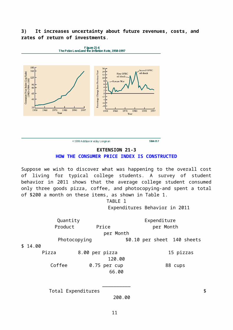
c) Intermediate case: when forecasts are partially correct, but even if forecasts are correct, it may be difficult to adjust for inflation because of binding contracts.* Indexation: is linking payments to changes in the general price level. It is away to go around inflation.Once again: Inflation is bad because:- 1) It erodes the purchasing power of money.2) It redistributes income in a haphazard way between people.3) It increases uncertainty about future revenues, costs, and rates of return of investments.
©1999 Addison Wesley Longman Slide 21.7
Figure 21-6The Price Level and the Inflation Rate, 1950-1997
EXTENSION 21-3
HOW THE CONSUMER PRICE INDEX IS CONSTRUCTED
Suppose we wish to discover what was happening to the overall cost of living for typical college students. A survey of student behavior in 2011 shows that the average college student consumed only three goods pizza, coffee, and photocopying-and spent a total of $200 a month on these items, as shown in Table 1.
TABLE l Expenditures Behavior in 2011
Quantity ExpenditureProduct Price per Month per Month
Photocopying $0.10 per sheet 140 sheets $ 14.00 Pizza 8.00 per pizza 15 pizzas 120.00 Coffee 0.75 per cup 88 cups 66.00 __________ Total Expenditures $ 200.00
By 2012, the price of photocopying has fallen to.0 5 cents per copy, the price of pizza has increased to $8.50, and the price of coffee has increased to 80 cents. What has happened to the cost of living? In order to find out, we calculate the cost of purchasing the 2011 bundle of goods at the prices that prevailed in 2012, as shown in Table 2.
9

TABLE 22011 Expenditures Behavior at 2012 Prices
Quantity Expenditures Product Price per Month per MonthPhotocopying $0.05 per sheet 140 sheets $ 7.00Pizza 8.50 per pizza 15 pizzas 127.00Coffee 0.80 per cup 88 cups 70.40 __________ Total Expenditures $204.90
The cost of living has increased by $ 4.90, or 2.45 %The base year (2011) figure is assigned an index number of 100. So, for 2012 the cost of living is 102.45For example, in May 1998 the CPI in the United States was 162.8 on a base of 1982-1984 (the period in which the original survey was done.) Thus, the price level had risen by 62.8 percent over the preceding 13 years, an average annual rate of increase of 3.82 percent.
The CPI is not a perfect measure of the cost of living because it does not account for quality improvements or for the tendency of consumers to purchase more of things whose prices fall, (and less of things whose prices rise). Also, it may not include new products. Thus, from time to time the underlying survey of consumer expenditure must be updated in order to keep up with changes in consumption patterns.
The Interest rate:-Is the price for lending and borrowing money. In reality, there are many interest rates. However, interest rates commonly move together. The height of the interest rate is affected by many factors (eg risk of customer, govt. fiscal and monetary policies, foreign interest rates… etc.).
* The prime interest rate: The rate banks charge to their best business customers.
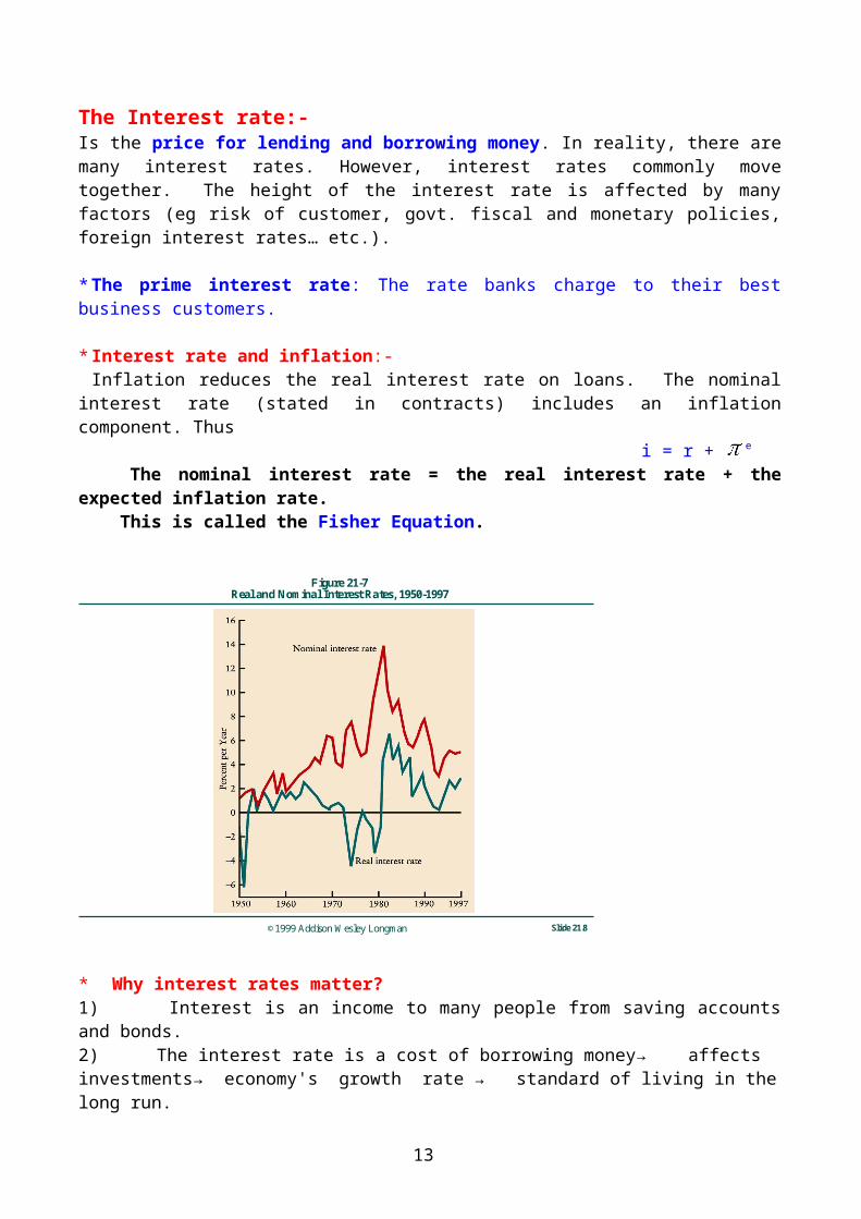
* Interest rate and inflation:-Inflation reduces the real interest rate on loans. The nominal interest rate (stated in contracts)
includes an inflation component. Thus i = r + e
The nominal interest rate = the real interest rate + the expected inflation rate. This is called the Fisher Equation.
10
©1999 Addison Wesley Longman Slide 21.8
Figure 21-7Real and Nominal Interest Rates, 1950-1997
* Why interest rates matter?1) Interest is an income to many people from saving accounts and bonds.2) The interest rate is a cost of borrowing money→ affects investments→ economy's growth rate → standard of living in the long run.3) It affects consumption & saving decisions.
In the short run the interest rate affects output and employment, & the business cycle. Note: Interest is Riba, and Riba is a major sin. We have to discuss it because it is a reality of the world, that we should work to eliminate.
International Economy:
1) The exchange rate: is the price of one currency in terms of another. Or, the No. of units of a local currency required to purchase one unit of a foreign currency (eg. SR3.75 = $1). So, according to this definition if the exchange rate ↑→ local currency depreciates. If the exchange rate ↓→ local currency appreciates.Note: the definition can be reversed. However, the above definition is the standard one.See Fig. 21-8, for the external value of the dollar. Why is it important to Saudi Arabia?
11
©1999 Addison Wesley Longman Slide 21.9
Figure 21-8The External Value of the U.S. Dollar, 1970-1997
Foreign exchange is the amount of foreign currency or claims on foreign currencies, such as foreign deposits, bonds and stocks that a country has.
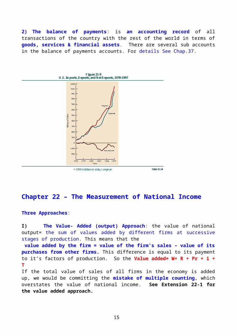
2) The balance of payments: is an accounting record of all transactions of the country with the rest of the world in terms of goods, services & financial assets. There are several sub accounts in the balance of payments accounts. For details See Chap.37.
©1999 Addison Wesley Longman Slide 21.10
Figure 21-9U.S. Imports, Exports, and Net Exports, 1970-1997
12
Chapter 22 – The Measurement of National Income
Three Approaches:
I) The Value- Added (output) Approach: the value of national output= the sum of values added by different firms at successive stages of production. This means that the value added by the firm = value of the firm's sales – value of its purchases from other firms. This difference is equal to its payment to it’s factors of production. So the Value added= W+ R + Pr + i + TIf the total value of sales of all firms in the economy is added up, we would be committing the mistake of multiple counting, which overstates the value of national income. See Extension 22-1 for the value added approach.
EXTENSION 22-1
VALUE ADDED THROUGH STAGES OF PRODUCTION
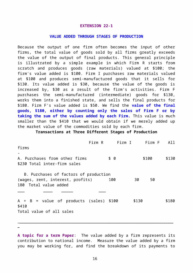
Because the output of one firm often becomes the input of other firms, the total value of goods sold by all firms greatly exceeds the value of the output of final products. This general principle is illustrated by a simple example in which Firm R starts from scratch and produces goods (raw materials) valued at $100; the firm's value added is $100. Firm I purchases raw materials valued at $100 and produces semi-manufactured goods that it sells for $130. Its value added is $30, because the value of the goods is increased by, $30 as a result of the firm's activities. Firm F purchases the semi-manufactured (intermediate) goods for $130, works them into a finished state, and sells the final products for $180. Firm F's value added is $50. We find the value of the final goods, $180, either by counting only the sales of Firm F or by taking the sum of the values added by each Firm. This value is much smaller than the $410 that we would obtain if we merely added up the market value of the commodities sold by each firm.
Transactions at Three Different Stages of Production
Firm R Firm I Firm F All firms-A. Purchases from other firms $ 0 $100 $130 $230 Total inter-firm sales
B. Purchases of factors of production(wages, rent, interest, profits) 100 30 50 180 Total value added
___ ____ _____ ___
A + B = value of products (sales) $100 $130 $180 $410 Total value of all sales
_________________________________________________________________________________
A topic for a term Paper: The value added by a firm represents its contribution to national income. Measure the value added by a firm you may be working for, and find the breakdown of its payments to its factors of production. Do the same for other firms in the same business sector and for several years. This should indicate to you the relative importance of the firm to the sector, and the relative importance of the sector to the national economy. Also, this should tell you something about the distribution of income between different owners of factors of production.
13

II) The Expenditures Approach: GDP is the sum of aggregate expenditures on final domestic goods and services. There are four components of expenditures:
a) Consumption: expenditures on final goods & services intended for immediate use during the year.b) Investment: expenditures on goods that aren’t for immediate consumption:i) inventory of raw materials, semi finished goods, and finished good. Inventories are recorded at market value. Inventory is part of investment because it is not intended to meet immediate consumption and there is tied up capital in it. Thus, there is an opportunity cost to hold inventory. Inventory reduction is an act of disinvestment.ii) plant and equipment: the economy’s stock of capital is a major source of economic growth.iii) residential housing: its services extend over many years - gross investment = replacement investment + net investment - Both investments are part of national income because in the process of producing each, factors of production are employed.
c) Govt. purchases of goods and services: expenditures generated in the process of output produced by the govt. involves hiring factors of production (e.g. schools, hospitals, roads, police and court services…. etc.) Govt. output is recorded at cost, (compare to inventory). This may understate or overstate govt. output depending on govt. efficiency.
d) Net exports: exports - importsimports: income generated by us to foreign producers. Thus, it must be deducted from national income. All previous national income components include an import component.Exports: income generated to us by foreign buyers, so it must be added to our income. THUS:Aggregate Expenditures (AE) = GDP= Consumption +Investment +Govt. Purchases + (Exports –Imports)
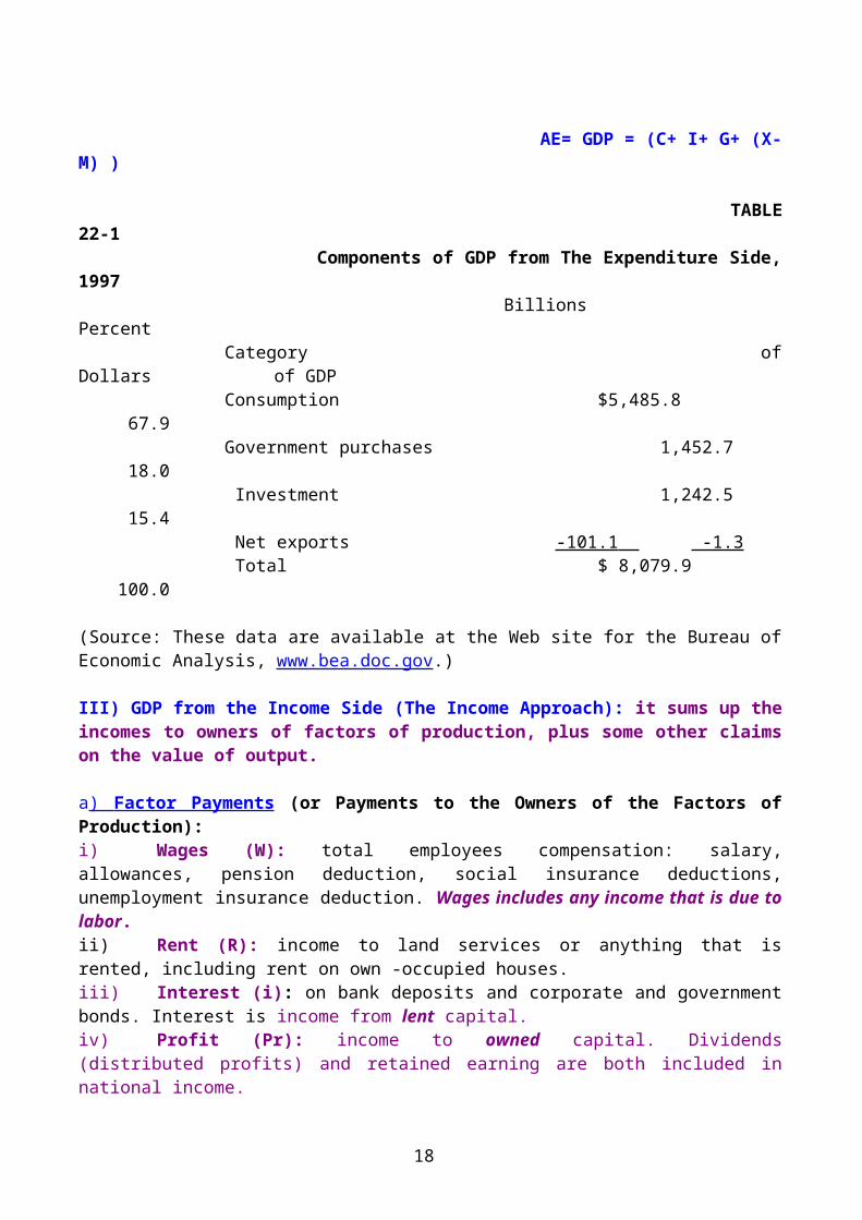
AE= GDP = (C+ I+ G+ (X-M) )
TABLE 22-1 Components of GDP from The Expenditure Side, 1997
Billions Percent Category of Dollars of GDP Consumption $5,485.8 67.9 Government purchases 1,452.7 18.0 Investment 1,242.5 15.4 Net exports -101.1 -1.3 Total $ 8,079.9 100.0
(Source: These data are available at the Web site for the Bureau of Economic Analysis, www.bea.doc.gov.)
III) GDP from the Income Side (The Income Approach): it sums up the incomes to owners of factors of production, plus some other claims on the value of output.
a) Factor Payments (or Payments to the Owners of the Factors of Production):i) Wages (W): total employees compensation: salary, allowances, pension deduction, social insurance deductions, unemployment insurance deduction. Wages includes any income that is due to labor.
14
ii) Rent (R): income to land services or anything that is rented, including rent on own -occupied houses.iii) Interest (i): on bank deposits and corporate and government bonds. Interest is income from lent capital.iv) Profit (Pr): income to owned capital. Dividends (distributed profits) and retained earning are both included in national income.
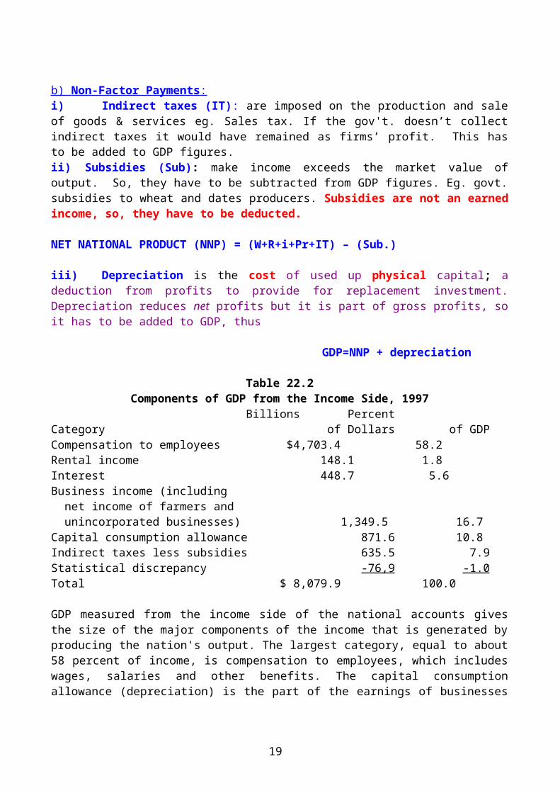
b) Non-Factor Payments : i) Indirect taxes (IT): are imposed on the production and sale of goods & services eg. Sales tax. If the gov't. doesn’t collect indirect taxes it would have remained as firms’ profit. This has to be added to GDP figures.ii) Subsidies (Sub): make income exceeds the market value of output. So, they have to be subtracted from GDP figures. Eg. govt. subsidies to wheat and dates producers. Subsidies are not an earned income, so, they have to be deducted.
NET NATIONAL PRODUCT (NNP) = (W+R+i+Pr+IT) – (Sub.)
iii) Depreciation is the cost of used up physical capital; a deduction from profits to provide for replacement investment. Depreciation reduces net profits but it is part of gross profits, so it has to be added to GDP, thus
GDP=NNP + depreciation
Table 22.2Components of GDP from the Income Side, 1997
Billions PercentCategory of Dollars of GDPCompensation to employees $4,703.4 58.2Rental income 148.1 1.8Interest 448.7 5.6Business income (including net income of farmers and unincorporated businesses) 1,349.5 16.7Capital consumption allowance 871.6 10.8Indirect taxes less subsidies 635.5 7.9Statistical discrepancy -76,9 -1.0Total $ 8,079.9 100.0
GDP measured from the income side of the national accounts gives the size of the major components of the income that is generated by producing the nation's output. The largest category, equal to about 58 percent of income, is compensation to employees, which includes wages, salaries and other benefits. The capital consumption allowance (depreciation) is the part of the earnings of businesses that is needed to replace capital used up during the year. This amounts to over 10 percent of GDP. (Source: Economic Report of the President, 1998.)
SEE SAMA's ANNUAL REPORT http://www.sama.gov.sa FOR NATIONAL INCOME ACCOUNTS OF SAUDI ARABIA, AND NOTE THE SIMILARITIES & DIFERECES WITH THE APPROACHES EXPLAINED IN THE TEXTBOOK.
* GDP (gross domestic product) is income produced at home.
15
GNP (gross national product) is income received at home+ net foreign incomeGNP=GDP+ (income to foreign investment locally – income from our international
investments)
Disposable national income (Y ):- How much of national is left to persons (the owners of the factors of production) to consume and save. It is the most important variable that affects consumption expend.
Y = GDP - IT - Dep.- RE (retained earnings)- i (paid to financial institutions) + Sub.+ TR
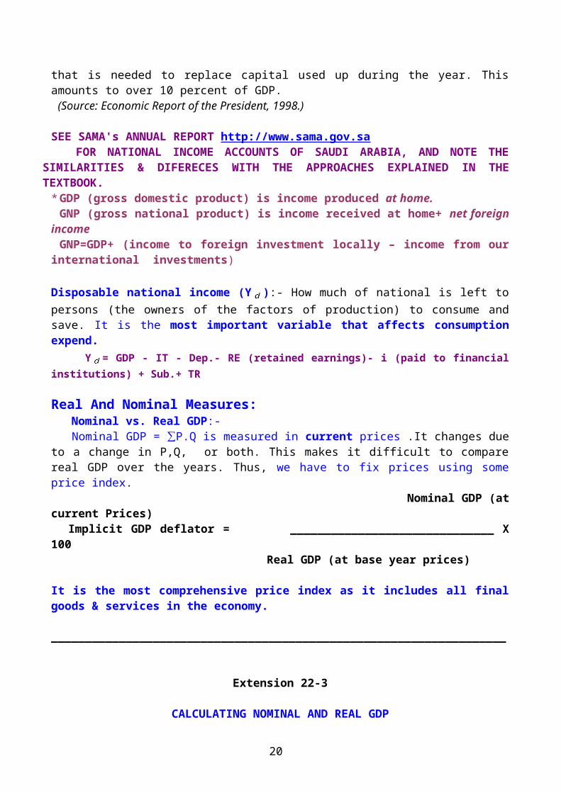
Real And Nominal Measures: Nominal vs. Real GDP:- Nominal GDP = ∑P.Q is measured in current prices .It changes due to a change in P,Q, or both. This makes it difficult to compare real GDP over the years. Thus, we have to fix prices using some price index. Nominal GDP (at current Prices) Implicit GDP deflator = ______________________________ X 100
Real GDP (at base year prices)
It is the most comprehensive price index as it includes all final goods & services in the economy. ___________________________________________________________________
Extension 22-3
CALCULATING NOMINAL AND REAL GDP
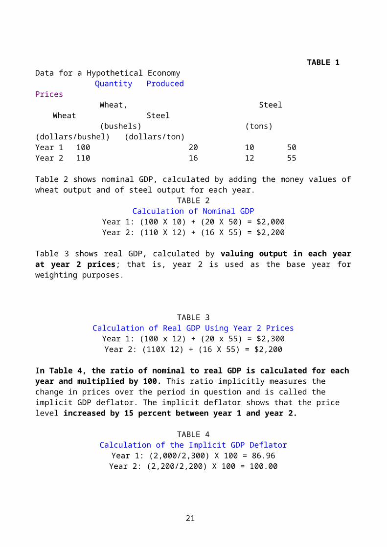
TABLE 1Data for a Hypothetical Economy
Quantity Produced Prices Wheat, Steel Wheat Steel (bushels) (tons) (dollars/bushel) (dollars/ton)
Year 1 100 20 10 50Year 2 110 16 12 55
Table 2 shows nominal GDP, calculated by adding the money values of wheat output and of steel output for each year.
TABLE 2Calculation of Nominal GDP
Year 1: (100 X 10) + (20 X 50) = $2,000Year 2: (110 X 12) + (16 X 55) = $2,200
Table 3 shows real GDP, calculated by valuing output in each year at year 2 prices; that is, year 2 is used as the base year for weighting purposes.
TABLE 3Calculation of Real GDP Using Year 2 Prices
16
Year 1: (100 x 12) + (20 x 55) = $2,300Year 2: (110X 12) + (16 X 55) = $2,200
In Table 4, the ratio of nominal to real GDP is calculated for each year and multiplied by 100. This ratio implicitly measures the change in prices over the period in question and is called the implicit GDP deflator. The implicit deflator shows that the price level increased by 15 percent between year 1 and year 2.
TABLE 4Calculation of the Implicit GDP Deflator
Year 1: (2,000/2,300) X 100 = 86.96Year 2: (2,200/2,200) X 100 = 100.00
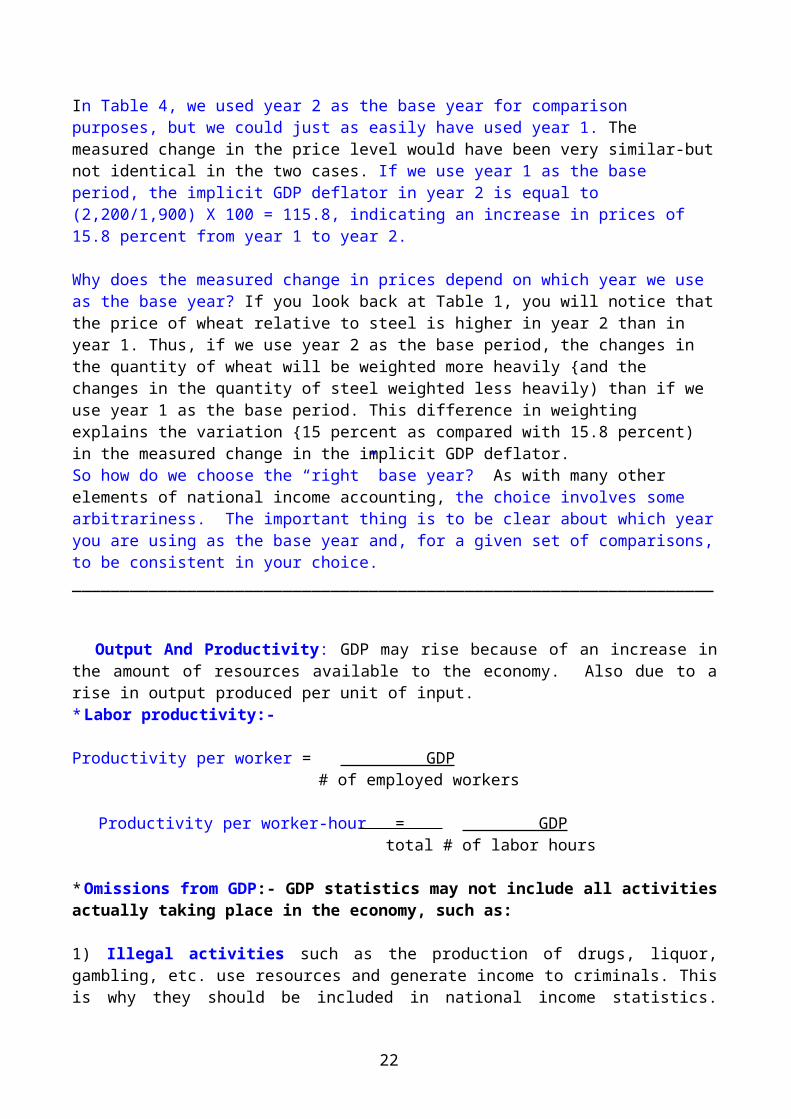
In Table 4, we used year 2 as the base year for comparison purposes, but we could just as easily have used year 1. The measured change in the price level would have been very similar-but not identical in the two cases. If we use year 1 as the base period, the implicit GDP deflator in year 2 is equal to (2,200/1,900) X 100 = 115.8, indicating an increase in prices of 15.8 percent from year 1 to year 2.
Why does the measured change in prices depend on which year we use as the base year? If you look back at Table 1, you will notice that the price of wheat relative to steel is higher in year 2 than in year 1. Thus, if we use year 2 as the base period, the changes in the quantity of wheat will be weighted more heavily {and the changes in the quantity of steel weighted less heavily) than if we use year 1 as the base period. This difference in weighting explains the variation {15 percent as compared with 15.8 percent) in the measured change in the implicit GDP deflator.So how do we choose the “right” base year? As with many other elements of national income accounting, the choice involves some arbitrariness. The important thing is to be clear about which year you are using as the base year and, for a given set of comparisons, to be consistent in your choice.___________________________________________________________________
Output And Productivity: GDP may rise because of an increase in the amount of resources available to the economy. Also due to a rise in output produced per unit of input.* Labor productivity:-
Productivity per worker = GDP # of employed workers
Productivity per worker-hour = GDP total # of labor hours
* Omissions from GDP:- GDP statistics may not include all activities actually taking place in the economy, such as:
1) Illegal activities such as the production of drugs, liquor, gambling, etc. use resources and generate income to criminals. This is why they should be included in national income statistics. However, this shouldn’t imply that their inclusion imply a rise in social welfare. Illegal activities harm society in 2 ways:
a) waste of resources in bad things
17
b) waste of resources in fighting crimes.Illegal activities may be reported in national income when legal activities are used as a cover for illegal ones.
2) Unreported activities: could be perfectly legal in themselves however people don’t report them to avoid taxes.
3) Non-market activities: includes “do –it- yourself” works, voluntary works, housewives' works, value of leisure. 4) Economic “bads” such as traffic congestions, pollution etc. (also when students park their cars in the professors' parking lots).
END OF CHAPTER 22
Chapter 23: National Income Determination: Part I
18
* National Income accounting deals with measuring actual expenditures while the theory of national income deals with how NI is determined. * Distinguish between actual & desired aggregate expenditure. EX: inventory is part of investment expenditures. The actual level of inventories maybe >,<,= intended ( desired) inventory,
Actual Expenditures =Ca + Ia +Ga + (Xa-Ma)Desired Expenditures= C+I+G+ (X-M)
* Simplifying assumptions for this Chapter:1) constant price level → no inflation2) no government → G=0,T=03) closed economy → X=0 , M=0
* Autonomous (Exogenous) variable: is a variable that cannot be explained by the model. In the theory of NI it is a variable not affected by national income. Autonomous expend. can and do change , but such changes do not occur systematically in response to changes in NI.* Induced (Endogenous) variable is one that can be explained by the model. i.e. is affected by NI.
* The consumption function relates desired consumption to the variables that affects it. In many countries, consumption is the largest single component of aggregate expenditures.
1) the most important factor that affects C is personal disposable income
if T=0 → disposable income (Yd) = National income(Y)
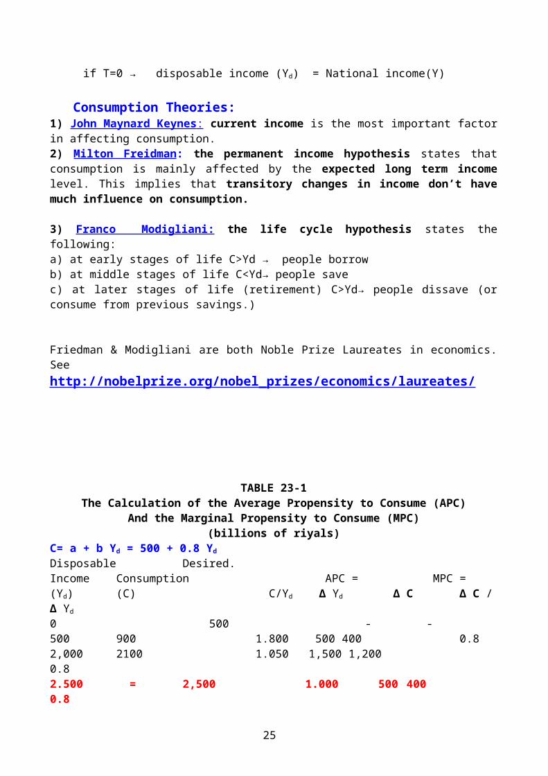
Consumption Theories:1) John Maynard Keynes : current income is the most important factor in affecting consumption.2) Milton Freidman: the permanent income hypothesis states that consumption is mainly affected by the expected long term income level. This implies that transitory changes in income don’t have much influence on consumption.
3) Franco Modigliani: the life cycle hypothesis states the following:a) at early stages of life C>Yd → people borrowb) at middle stages of life C<Yd→ people savec) at later stages of life (retirement) C>Yd→ people dissave (or consume from previous savings.)
Friedman & Modigliani are both Noble Prize Laureates in economics. Seehttp://nobelprize.org/nobel_prizes/economics/laureates/
TABLE 23-1The Calculation of the Average Propensity to Consume (APC)
And the Marginal Propensity to Consume (MPC)
19
(billions of riyals)C= a + b Yd = 500 + 0.8 Yd
Disposable Desired.Income Consumption APC = MPC =(Yd) (C) C/Yd Δ Yd Δ C Δ C / Δ Yd 0 500 - -500 900 1.800 500 400 0.82,000 2100 1.050 1,500 1,200 0.82.500 = 2,500 1.000 500 400 0.85,000 4,500 0.900 2,500 2,000 0.87,500 6,500 0.867 2,500 2,000 0.88,750 7,500 0.857 1,250 1,000 0.810,000 8,500 0.850 1,250 1,000 0.8
APC measures the proportion of disposable income that households desire to spend on consumption; MPC measures the proportion of any increment to disposable income that households desire to spend on consumption. The data are hypothetical. Economists call the level of income at which desired consumption equals disposable income the break-even level; in this example it is $2,500 billion. APC, calculated in the third column, exceeds 1-that is, consumption exceeds income below the break-even level. Above the break-even level, APC is less than 1. It is negatively related to income at all levels of income. MPC, equals 0.80 at all levels of Yd. Thus in this example 80 halalah of every additional riyal of disposable income is spent on consumption, and 20 halalah is saved.___________________________________________________________________
* the average propensity to consume ( APC) = total consumption = C/ Y total income
the marginal propensity to consume ( MPC) = change in Consumption = Δ C change in income Δ Y
In other words, MPC is the slop of the linear consumption function.
20
©1999 Addison Wesley Longman Slide 23.2
Figure 23-1The Consumption and Saving Functions
The Saving Function: The Average Propensity to Save (APS) =S/Yd The Marginal Propensity to Save (MPS) = S/ Yd
TABLE 23-2Consumption and Saving Schedules
(billions of dollars)
Disposable Desired Desired Income Consumption Saving0 500 -500500 900 -4002,000 2,100 -1002,500 2,500 05,000 4,500 5007,500 6,500 1,0008,750 7,500 1,25010,000 8,500 1,500
Saving and consumption account for all household disposable income. The first two columns repeat the data from Table 23-1. The third column, desired saving, is disposable income minus desired consumption. Consumption and saving both increase steadily as disposable income rises. In this example, the break-even level of disposable income is $2,500 billion; thus desired saving is zero at this point.
APC+ APS =1
21
MPC+ MPS = 1C=a + b Y ; S = -a + (1-b) Yd
Where a: is autonomous consumption. bY is induced consumption. , b is the slop of a linear cons. FunctionThe 45- degree Line: points on that line imply C= Y (spending equals income) no saving
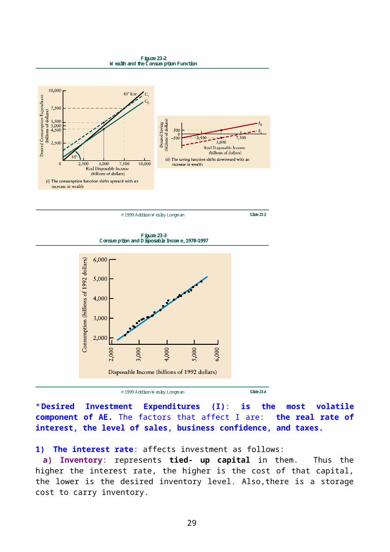
* consumption & wealth: a rise in wealth ( a stock concept, a concept that has no time dimension) increases the flow of consumption out of a given level of income. Moreover, it reduces the flow of saving out of that income. A rise in wealth shifts the consumption function upwards while it shifts the S- function downward. SEE Fig 23-2.
©1999 Addison Wesley Longman Slide 23.3
Figure 23-2Wealth and the Consumption Function
22
©1999 Addison Wesley Longman Slide 23.4
Figure 23-3Consumption and Disposable Income, 1970-1997
* Desired Investment Expenditures (I): is the most volatile component of AE. The factors that affect I are: the real rate of interest, the level of sales, business confidence, and taxes.
1) The interest rate: affects investment as follows: a) Inventory: represents tied- up capital in them. Thus the higher the interest rate, the higher is the cost of that capital, the lower is the desired inventory level. Also,there is a storage cost to carry inventory.b) Residential housing: the interest component of the cost of housing could represent a very large percentage of the total cost of a house.c) Plant and equipment: firms finance some or all capital expansion by retained earnings. The higher the interest, the less will be the desire to go for debt, and the more attractive is financial investment (the less attractive is real investment.) 2) The level of sales:a) Inventory levels: change with the level of sales and level of production.b) If there is a surge in sales (demand) that firms believe is sustainable enough, they will invest in plant & equipment. However, once that is completed, investment decreases.3) Business confidence: is a psychological factor that could change in either direction for many different reasons. It is a major source of investment volatility.4) Taxes: reduce profits and thus a cost that affects investments in plant & equipment. Governments give special tax reductions to encourage both domestic and foreign investment.* The role of profits in the economy.1) They are signals that direct resources into their best use (assuming perfect markets). 2) Profits help to payback for the cost of existing investments. 3) Profits help to finance future investments. 4) Profits pay for taxes and interest.In the Islamic system, interst is not allowed, and Zakat is not related to profits * For simplicity: investments will be assumed to be autonomous. Thus I = * This chapter assumes G=T=X=M=0 , thus
23
* THE AGGREGATE EXPENDITURE FUNCTION IS AE=C+
AE= a + by + In this simple economy, the marginal propensity to spend out of national income ( Z) is the
same as mpc (b ) ; (1-z) is the marginal propensity not to spend) is the same as the MPS.
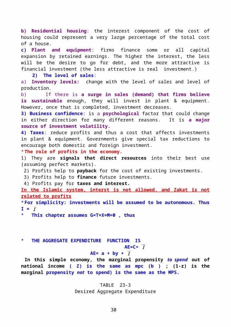
TABLE 23-3Desired Aggregate Expenditure
(billions of dollars)
Desired Consumption Desired
Desired Aggregate National Expenditure Investment Expenditure
Income (C = 500 +0.8Y) Expenditure (Y) (I = 1,250) (AE= C + I) 0 500 1250 1750 500 900 1,250 2,150 2,000 2,100 1,250 3,350 2,500 2,500 1,250 3,750 5,000 4,500 1,250 5,750 7,500 6,500 1,250 7,750 8,750 7,500 1,250 8,750 10,000 8,500 1,250 9,750 15,000 12,500 1,250 13,750
In a simple economy with no government and no international trade, desired aggregate expenditure is the sum of desired consumption and desired investment. In this table government and net exports are assumed to be zero, desired investment is assumed to be constant at $1,250 billion, and desired consumption is based on the hypothetical data given in Table 23-1. The autonomous components of desired aggregate expenditure are desired investment the constant term in desired consumption expenditure. The induced component is the second term in desired consumption expenditure (0.8 Y).
24
©1999 Addison Wesley Longman Slide 23.5
Figure 23-4The Aggregate Expenditure Function
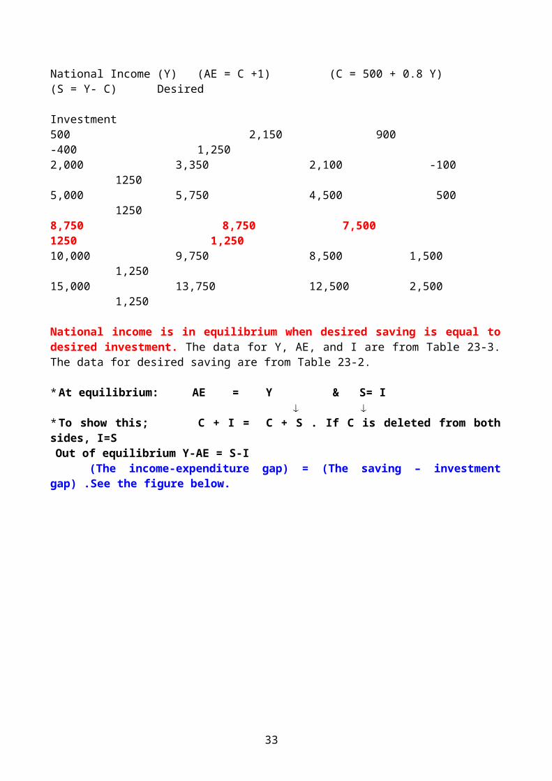
* Determination of equilibrium NI:1) if AE>Y → pressure an income to rise.2) If AE<y → pressure an income to decrease.3) Equilibrium will be achieved where AE=Y
TABLE 23-5The Saving-Investment Balance
Desired Aggregate Expenditure Desired Consumption Desired Saving
National Income (Y) (AE = C +1) (C = 500 + 0.8 Y) (S = Y- C) Desired Investment 500 2,150 900 -400 1,2502,000 3,350 2,100 -100 1250 5,000 5,750 4,500 500 12508,750 8,750 7,500 1250 1,25010,000 9,750 8,500 1,500 1,25015,000 13,750 12,500 2,500 1,250
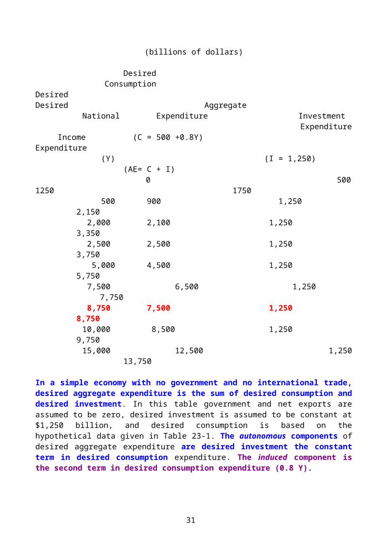
National income is in equilibrium when desired saving is equal to desired investment. The data for Y, AE, and I are from Table 23-3. The data for desired saving are from Table 23-2.
* At equilibrium: AE = Y & S= I * To show this; C + I = C + S . If C is deleted from both sides, I=S
Out of equilibrium Y-AE = S-I (The income-expenditure gap) = (The saving – investment gap) .See the figure below.
25

©1999 Addison Wesley Longman Slide 23.6
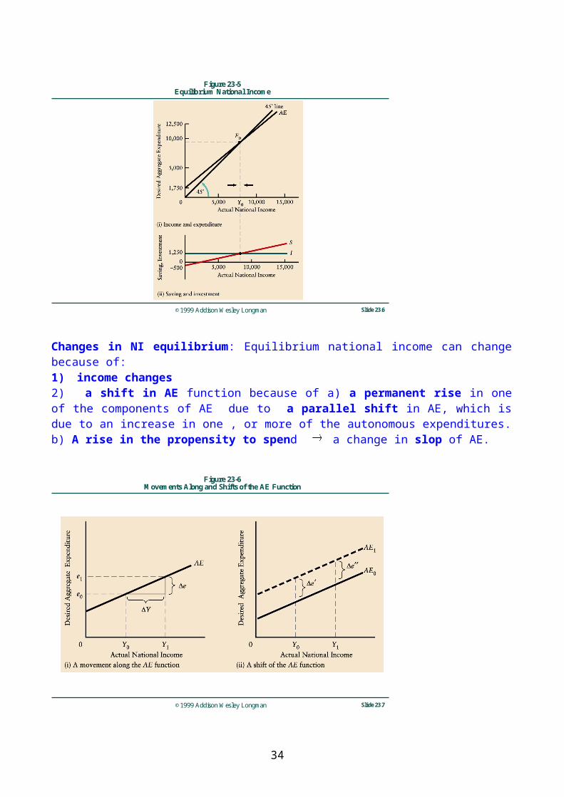
Figure 23-5Equilibrium National Income
Changes in NI equilibrium: Equilibrium national income can change because of: 1) income changes 2) a shift in AE function because of a) a permanent rise in one of the components of AE due to a parallel shift in AE, which is due to an increase in one , or more of the autonomous expenditures. b) A rise in the propensity to spend a change in slop of AE.
©1999 Addison Wesley Longman Slide 23.7
Figure 23-6Movements Along and Shifts of the AE Function
26

©1999 Addison Wesley Longman Slide 23.8
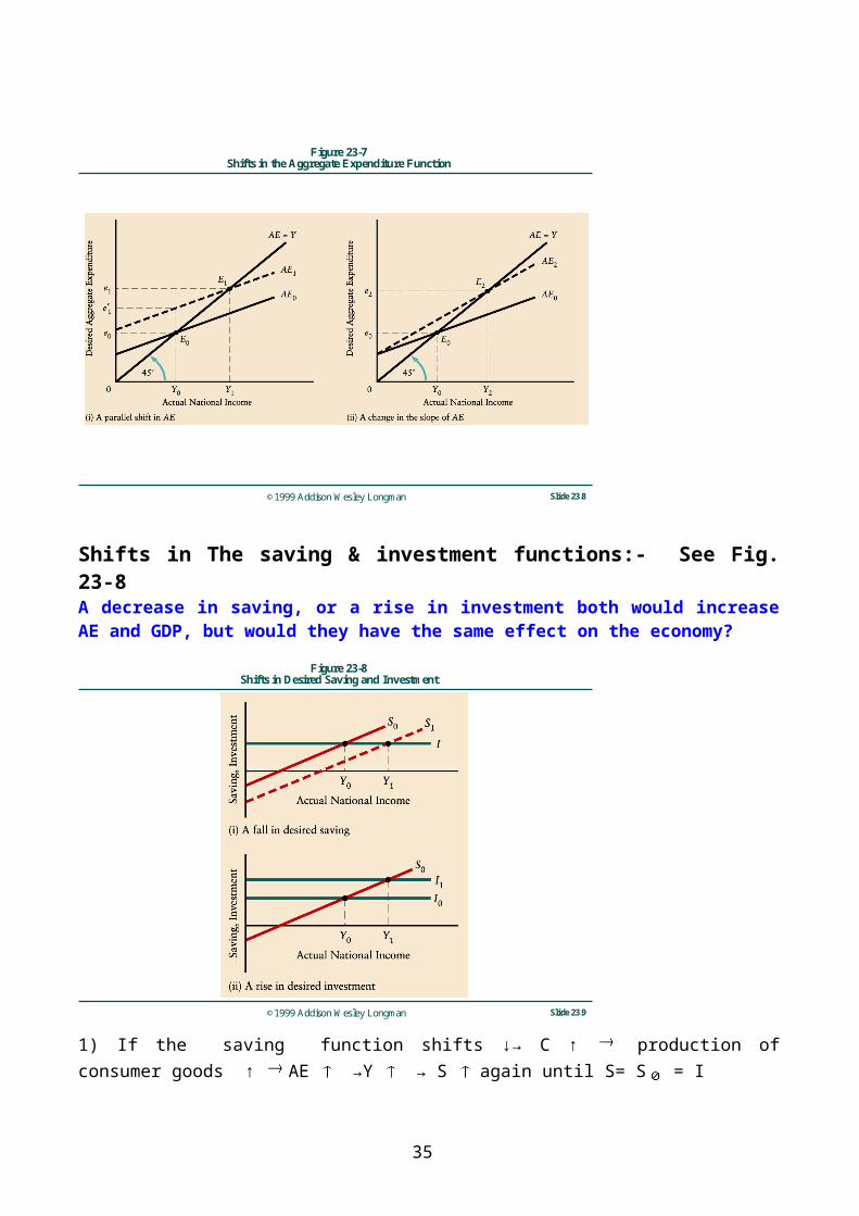
Figure 23-7Shifts in the Aggregate Expenditure Function
Shifts in The saving & investment functions:- See Fig. 23-8A decrease in saving, or a rise in investment both would increase AE and GDP, but would they have the same effect on the economy?
©1999 Addison Wesley Longman Slide 23.9
Figure 23-8Shifts in Desired Saving and Investment
1) If the saving function shifts ↓→ C ↑ production of consumer goods ↑ AE →Y → S again until S= S = I
In the final equilib. Y, C both rise, but S is the same. The Production of consumer goods increases.2) If the investments function shifts ↑ → AE ↑ → Y↑ → C↑& S↑→ in the final equilibrium Y , C, I,S all rise and the production of both investment and consumer goods↑
27

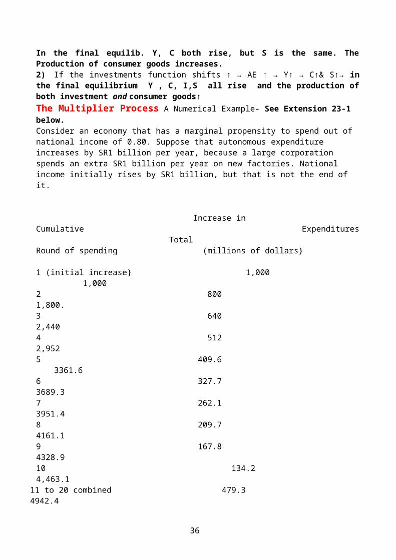
The Multiplier Process A Numerical Example- See Extension 23-1 below.Consider an economy that has a marginal propensity to spend out of national income of 0.80. Suppose that autonomous expenditure increases by SR1 billion per year, because a large corporation spends an extra SR1 billion per year on new factories. National income initially rises by SR1 billion, but that is not the end of it.
Increase in Cumulative Expenditures Total
Round of spending (millions of dollars}
1 (initial increase} 1,000 1,0002 800 1,800.3 640 2,4404 512 2,9525 409.6 3361.6 6 327.7 3689.3
7 262.1 3951.4
8 209.7 4161.1
9 167.8 4328.9 10 134.2 4,463.1
11 to 20 combined 479.3 4942.4All others 57.6 5000.0
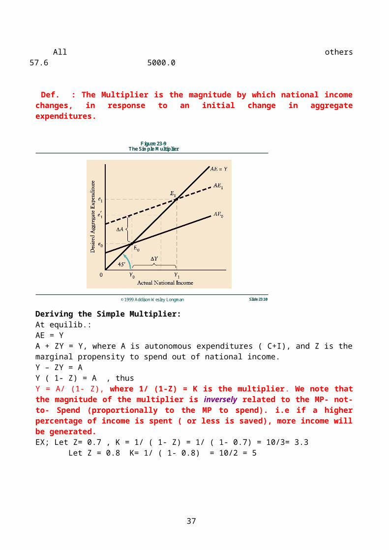
Def. : The Multiplier is the magnitude by which national income changes, in response to an initial change in aggregate expenditures.
28
©1999 Addison Wesley Longman Slide 23.10
Figure 23-9The Simple Multiplier
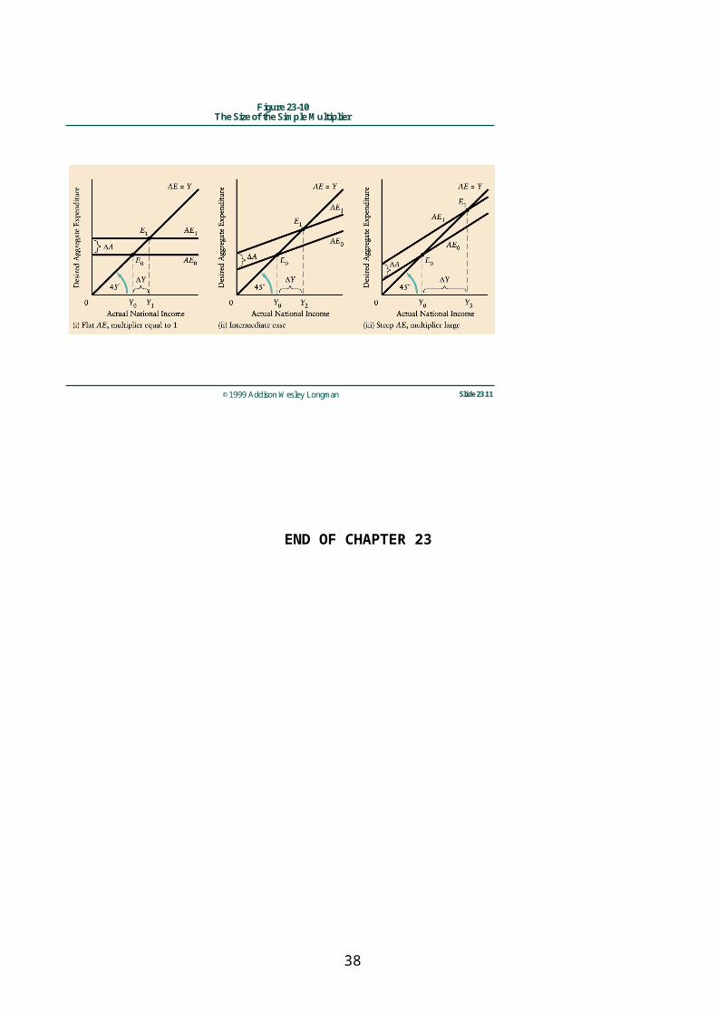
Deriving the Simple Multiplier:At equilib.:AE = YA + ZY = Y, where A is autonomous expenditures ( C+I), and Z is the marginal propensity to spend out of national income.Y – ZY = AY ( 1- Z) = A , thusY = A/ (1- Z), where 1/ (1-Z) = K is the multiplier. We note that the magnitude of the multiplier is inversely related to the MP- not-to- Spend (proportionally to the MP to spend). i.e if a higher percentage of income is spent ( or less is saved), more income will be generated.EX; Let Z= 0.7 , K = 1/ ( 1- Z) = 1/ ( 1- 0.7) = 10/3= 3.3 Let Z = 0.8 K= 1/ ( 1- 0.8) = 10/2 = 5
29
©1999 Addison Wesley Longman Slide 23.11
Figure 23-10The Size of the Simple Multiplier
END OF CHAPTER 23
30
REVIEW: End of Chapter QuestionsCh. 211)a) micro, particular marketb) macro, inflation, unemploymentc) macro, industrial productiond) macro, subsidies affect national income, but micro pricese) macro, recessionf)labor force expanding from population growth > a rise of employment =unemployment will rise
Ch. 225)
a) yes, consumptionb) yes, consumptionc) no, it in the contrary , spending an investmentd) no , transfer of titlee) yes, inventories part of investmentsf) no, ready counted when first sold
2) GDP not affected directly, but GNP is because income will go to foreigners not to “nationals”
GNP= GDP +Net Foreign income(not affected but transfers income to foreign ownership)
Ch. 23
1)c) upward shifts of C, and AE while saving shifts down d) AE, and I shifts downwardse) Investments decrease (reducing production, selling inventories until it waves out)f)If the government expending imports, export, (=consumption, I-gives investment C=1400+0.8y, I=400, equilib. Y=?, what will happen if interest rate ↑ ?
A) AE=C+I → 1400+0.8y + 400 = 1800+0.8y at equilibrium:AE=Y Y= 1800+0.8y → Y(1-0.8) = 1800 → Y=9000C=1400 +0.8 (9000) = 8600 S=Y-C= 9000-8600 = 400
Chapter 24: National Income Determination: Part II: Introducing Govt. & the Foreign Sector
31

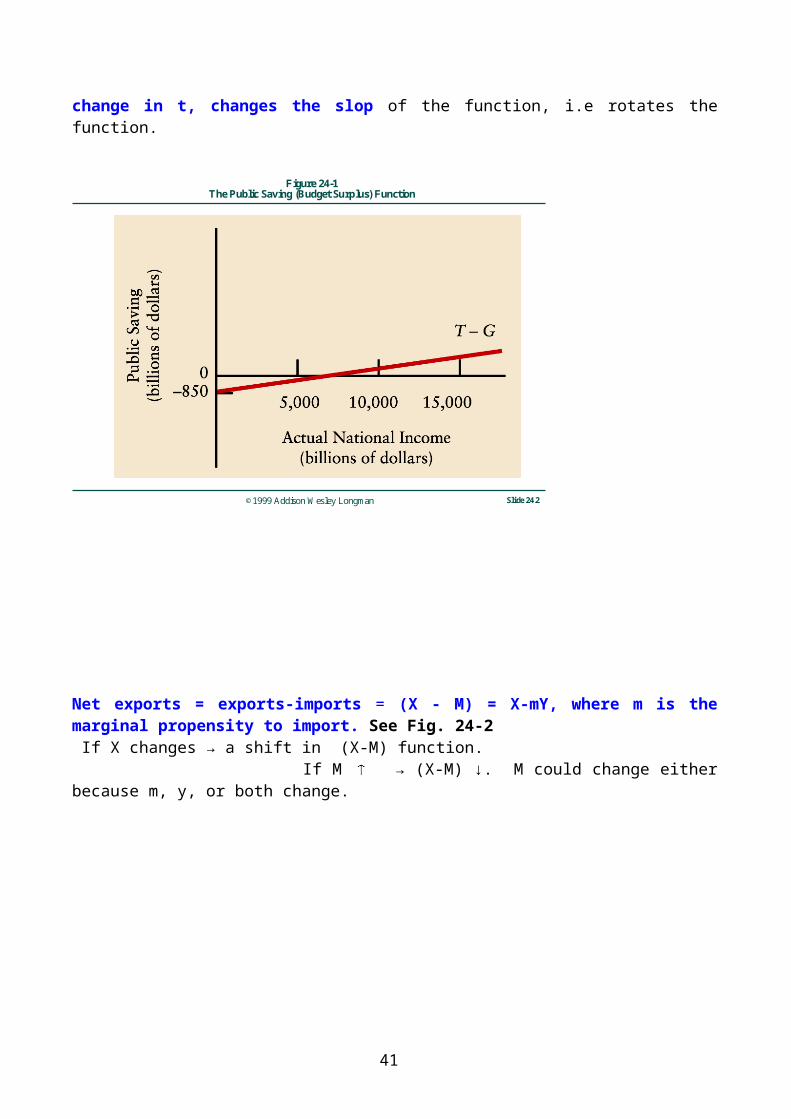
* Definition: Fiscal policy is the govt. policy regarding govt. expenditures and taxation.* When govt. is introduced into the model, Yd ≠ Y Yd = Y-T, also C ≠ f(Y), but C = f (Yd (Y)) → relationship between consumption & national income becomes indirect.* Net taxes T –TR = Taxes - Transfer Payments* Govt. spending includes govt. purchases (G) and Gov't Budget = G+TR.Notice TR is part of the Gov't budget, but not a gov't purchase of goods & services. So, TR is not part of G, but it affects AE & Y indirectly through Yd and C. The budget balance = T-G > 0 a surplus < 0 a deficit = 0 a balanced budget * The public saving function: T- G = tY - G , where G an is autonomous variable, t (tax rate) is also autonomous. The budget balance is positively related to national income (Y). t is the slope, and a change in G shifts the function parallel to itself. A change in t, changes the slop of the function, i.e rotates the function.
©1999 Addison Wesley Longman Slide 24.2
Figure 24-1The Public Saving (Budget Surplus) Function
Net exports = exports-imports = (X - M) = X-mY, where m is the marginal propensity to import. See Fig. 24-2 If X changes → a shift in (X-M) function. If M → (X-M) ↓. M could change either because m, y, or both change.
32
©1999 Addison Wesley Longman Slide 24.3
Figure 24-2The Net Export Function
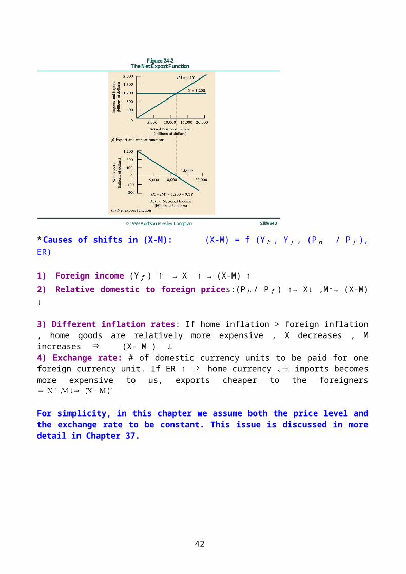
* Causes of shifts in (X-M): (X-M) = f (Y , Y , (P / P ), ER)
1) Foreign income (Y ) → X ↑ → (X-M) ↑ 2) Relative domestic to foreign prices:(P / P ) ↑→ X↓ ,M↑→ (X-M) ↓
3) Different inflation rates: If home inflation > foreign inflation , home goods are relatively more expensive , X decreases , M increases (X- M ) 4) Exchange rate: # of domestic currency units to be paid for one foreign currency unit. If ER ↑ home currency imports becomes more expensive to us, exports cheaper to the foreigners
For simplicity, in this chapter we assume both the price level and the exchange rate to be constant. This issue is discussed in more detail in Chapter 37.
33
©1999 Addison Wesley Longman Slide 24.4
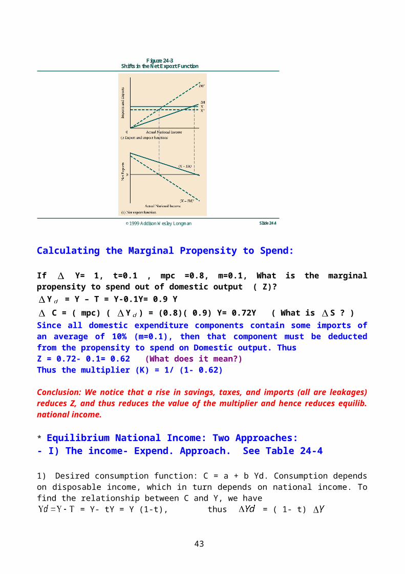
Figure 24-3Shifts in the Net Export Function
Calculating the Marginal Propensity to Spend:
If Y= 1, t=0.1 , mpc =0.8, m=0.1, What is the marginal propensity to spend out of domestic output ( Z)?
Y = Y – T = Y-0.1Y= 0.9 Y C = ( mpc) ( Y ) = (0.8)( 0.9) Y= 0.72Y ( What is S ? )
Since all domestic expenditure components contain some imports of an average of 10% (m=0.1), then that component must be deducted from the propensity to spend on Domestic output. Thus Z = 0.72- 0.1= 0.62 (What does it mean?)Thus the multiplier (K) = 1/ (1- 0.62)
Conclusion: We notice that a rise in savings, taxes, and imports (all are leakages) reduces Z, and thus reduces the value of the multiplier and hence reduces equilib. national income.
* Equilibrium National Income: Two Approaches:- I) The income- Expend. Approach. See Table 24-4
1) Desired consumption function: C = a + b Yd. Consumption depends on disposable income, which in turn depends on national income. To find the relationship between C and Y, we have
= Y- tY = Y (1-t), thus = ( 1- t)
We have C = a + b (1-t) Y:
/ = (mpc) (1-t ) = ( ) ( / Y ) assume a=500, mpc = / =0.8. Also assume t= 0.1. Thus
34
= 500+ 0.72Y
©1999 Addison Wesley Longman Slide 24.5
Figure 24-4The Aggregate Expenditure Funnction
©1999 Addison Wesley Longman Slide 24.6
Figure 24-5Equilibrium National Income
Thus: Equilib. is established where Y = AE = C + I +G+ ( X- M)
II) The Saving –Investment Approach: Another app. is to show that equilib. is attained where national saving = national investment. To show this we have to discuss the national saving & national investment functions first.The National Saving Function is the sum of private and public (govt.) savings functions: = S + ( T- G) ( Fig.24-6)
35
The slop of this function is the sum of the slops of private and public functions.
©1999 Addison Wesley Longman Slide 24.7
Figure 24-6The National Saving Function
Derivation of the slop: Keeping in mind that C=a+ bY S= -a + ( 1- b) Y S = -a+ (1 –b)( 1-t) Y
And T- G = tY – G
Thus the slop of the national saving function: (S + (T-G))/ Y = (1-b) (1-t) + t
So, if mpc= 0.8 & t = 0.1 , then mps=(1-mpc)= ( 1- b)= 0.2The slop of the national saving function is = (0.2)(0.9)+ 0.1=0.28
National Asset Formation (National Investment):This is equal to investment at home plus net claims on assets the country owns abroad. The latter comes from net exports and our net foreign investments. Thus:
National Asset Formation= I + (X –M)
Investment and exports have in common that both are not intended to meet current domestic consumption. A country that has positive net exports adds to its foreign assets, and thus is a net creditor. Negative net exports imply that the country is a net debtor.
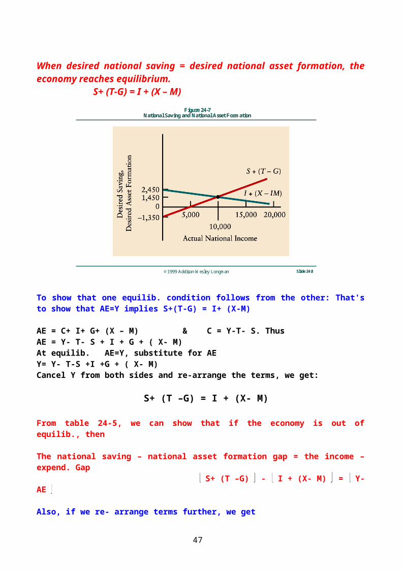
When desired national saving = desired national asset formation, the economy reaches equilibrium. S+ (T-G) = I + (X – M)
36
©1999 Addison Wesley Longman Slide 24.8
Figure 24-7National Saving and National Asset Formation
To show that one equilib. condition follows from the other: That's to show that AE=Y implies S+(T-G) = I+ (X-M)
AE = C+ I+ G+ (X – M) & C = Y-T- S. ThusAE = Y- T- S + I + G + ( X- M)At equilib. AE=Y, substitute for AEY= Y- T-S +I +G + ( X- M)Cancel Y from both sides and re-arrange the terms, we get:
S+ (T –G) = I + (X- M)
From table 24-5, we can show that if the economy is out of equilib., then
The national saving – national asset formation gap = the income – expend. Gap S+ (T –G) - I + (X- M) = Y- AE
Also, if we re- arrange terms further, we get S+T+M = I+ G+ X The Sum of Leakages = The Sum of Injections
Conclusion: There are three equivalent ways to express macroeconomic equilibrium. Can you re-state them?
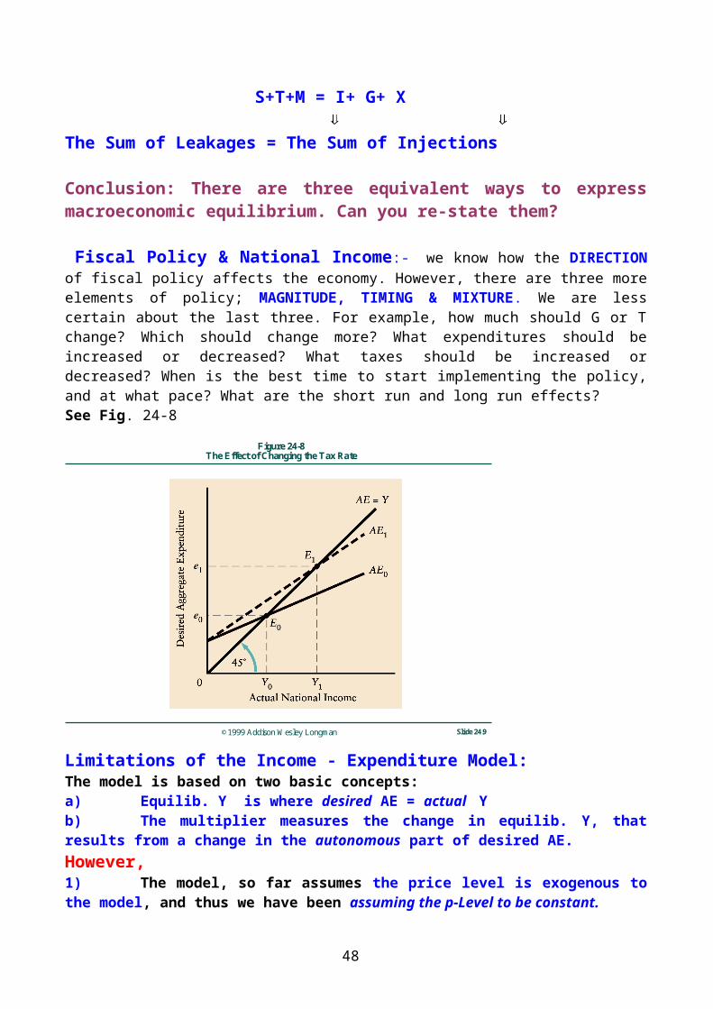
Fiscal Policy & National Income:- we know how the DIRECTION of fiscal policy affects the economy. However, there are three more elements of policy; MAGNITUDE, TIMING & MIXTURE. We are less certain about the last three. For example, how much should G or T change? Which should change more? What expenditures should be
37
increased or decreased? What taxes should be increased or decreased? When is the best time to start implementing the policy, and at what pace? What are the short run and long run effects?See Fig. 24-8
©1999 Addison Wesley Longman Slide 24.9
Figure 24-8The Effect of Changing the Tax Rate
Limitations of the Income - Expenditure Model:The model is based on two basic concepts:a) Equilib. Y is where desired AE = actual Yb) The multiplier measures the change in equilib. Y, that results from a change in the autonomous part of desired AE.However, 1) The model, so far assumes the price level is exogenous to the model, and thus we have been assuming the p-Level to be constant.2) It assumes that equilib. Y depends only on aggregate demand ( desired AE), and not on ( for example) on the firms’ technical capabilities, the supply of resources. 3) It assumes the economy has some unemployed resources, which means that a rise in AE , will generate a rise in real YThese assumptions imply that equilib. income is determined by the demand side of the economy alone. Income is said to be demand- determined.
Nevertheless, no matter what the p-Level is, the model continues to be useful to study the relationship between AE and Y. The equilib. conditions stated before still hold.
Deriving the Full Multiplier Model: Appendix Material; V.V. Imp.
38
C= a + b d
At Equilib. we have:
AE= Y, substitute for AE in the above AE function,
Y=C+I+G+ (X-M)Substitute for C,I, G,X, & M from the above,
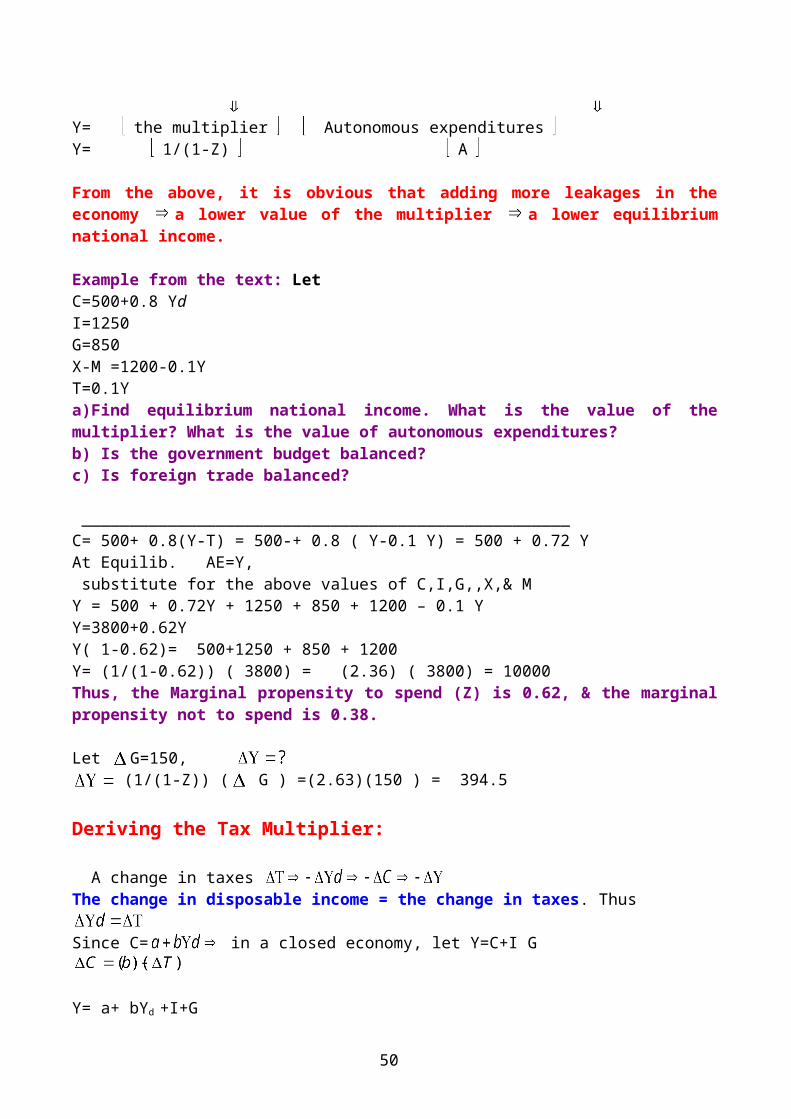
Y= 1/( 1-b+bt+m) Y= the multiplier Autonomous expendituresY= 1/(1-Z) A
From the above, it is obvious that adding more leakages in the economy a lower value of the multiplier a lower equilibrium national income.
Example from the text: LetC=500+0.8 YdI=1250G=850X-M =1200-0.1YT=0.1Ya)Find equilibrium national income. What is the value of the multiplier? What is the value of autonomous expenditures?b) Is the government budget balanced?c) Is foreign trade balanced? ___________________________________________________C= 500+ 0.8(Y-T) = 500-+ 0.8 ( Y-0.1 Y) = 500 + 0.72 YAt Equilib. AE=Y, substitute for the above values of C,I,G,,X,& MY = 500 + 0.72Y + 1250 + 850 + 1200 – 0.1 YY=3800+0.62YY( 1-0.62)= 500+1250 + 850 + 1200Y= (1/(1-0.62)) ( 3800) = (2.36) ( 3800) = 10000Thus, the Marginal propensity to spend (Z) is 0.62, & the marginal propensity not to spend is 0.38.
Let G=150,
39
(1/(1-Z)) ( G ) =(2.63)(150 ) = 394.5
Deriving the Tax Multiplier:
A change in taxes The change in disposable income = the change in taxes. Thus
Since C= in a closed economy, let Y=C+I G
Y= a+ bYd +I+GY= a+ b(Y-T) +I+G Y= a+bY- bT +I+G Y(1-b) = a- bT +I + G
Thus Y= ( ) ( a-bT +I+G)
(Expend. multiplier,K)
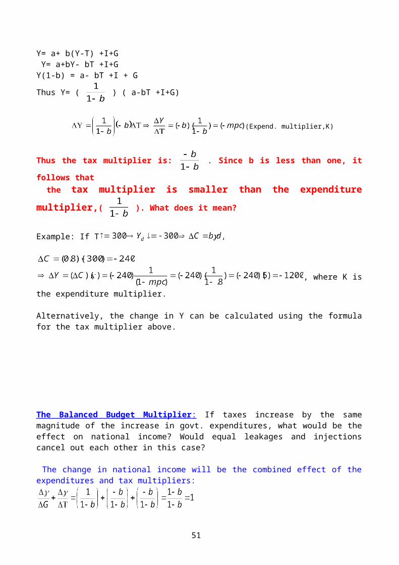
Thus the tax multiplier is: . Since b is less than one, it follows that
the tax multiplier is smaller than the expenditure multiplier,( ). What does it
mean?
Example: If T
, where K is the
expenditure multiplier.
Alternatively, the change in Y can be calculated using the formula for the tax multiplier above.
The Balanced Budget Multiplier : If taxes increase by the same magnitude of the increase in govt. expenditures, what would be the effect on national income? Would equal leakages and injections cancel out each other in this case?
The change in national income will be the combined effect of the expenditures and tax multipliers:
40
This implies that the balanced budget multiplier, in a closed economy is equal to1. Thus a balanced budget policy increases national income by the same amount of G = T.WHY? Can you explain?
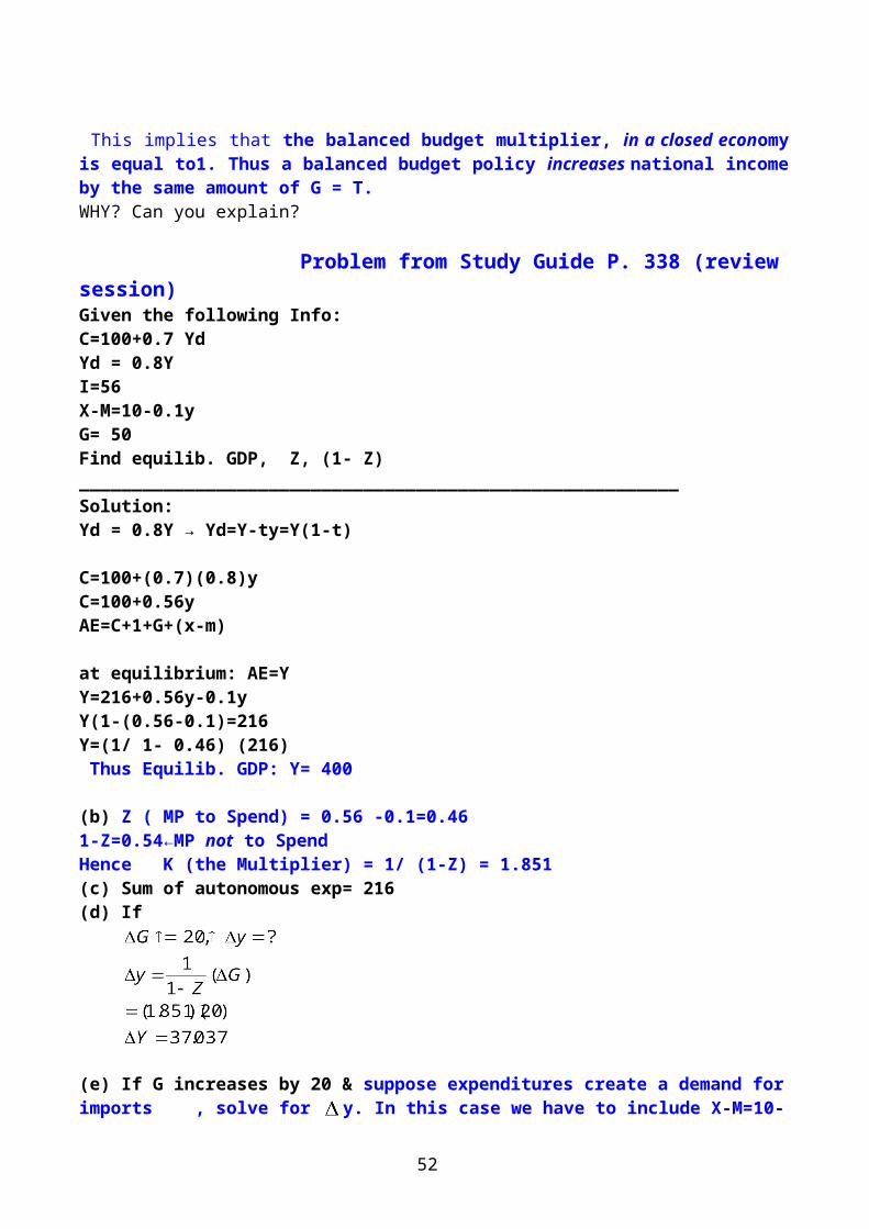
Problem from Study Guide P. 338 (review session)Given the following Info:C=100+0.7 YdYd = 0.8Y I=56X-M=10-0.1yG= 50Find equilib. GDP, Z, (1- Z) _________________________________________________________Solution:Yd = 0.8Y → Yd=Y-ty=Y(1-t)
C=100+(0.7)(0.8)yC=100+0.56yAE=C+1+G+(x-m)
at equilibrium: AE=YY=216+0.56y-0.1yY(1-(0.56-0.1)=216Y=(1/ 1- 0.46) (216) Thus Equilib. GDP: Y= 400
(b) Z ( MP to Spend) = 0.56 -0.1=0.461-Z=0.54←MP not to SpendHence K (the Multiplier) = 1/ (1-Z) = 1.851(c) Sum of autonomous exp= 216(d) If
(e) If G increases by 20 & suppose expenditures create a demand for imports , solve for y. In this case we have to include X-M=10-0.1Y. The final increase in Y will be reduced by 0.1 of the change in income that resulted from G. That is Y is reduced by 3.7 relative to part (d) above.
Why We need Equilibrium Analysis; Cartoon by Paul Krugman, The new York Times, October 1,2010.
41
Chap.25: Output and Prices in the Short Run
Virtually all AS & AD shocks affect both national income and the price level; that is they have both nominal and real effects. To understand these effects we have to drop the assumption of a constant price level that we maintained in the previous chapters.
The Demand Side of the Economy: Shifts in the AE function:
42
One Key Result: A rise in the P- level shifts the AE function down, and a fall in P- level shifts AE function up. WHY?
I) P-level & Changes in Consumption: Two links:
a) P → Wealth → C . Much of persons' private wealth is the form of assets with fixed nominal value: money and bonds. A rise in P-level reduces the purchasing power of money (M/P) → money wealth ↓ → real AE↓. Also, govt. and corporate bonds are fixed in nominal terms. A rise in P – level reduces real repayment to the bondholders (B/P) → wealth of bondholders ↓. However, for the bond issuer, since real repayment is lower → his real wealth ↑ → No net change in aggregate wealth of, assuming that both sides have the same mpc. b) P → Wealth → S → C. When wealth is decreased due to a rise in P – level, people need to increase their savings to restore their wealth to their desired level → Consumption ↓ → AE ↓.The above is the direct effect of wealth on consumption. There is an indirect effect that operates through the interest rate. It will be discussed in Chap.28. II) P –Level & Changes in Net Exports: A rise in domestic P-level → prices of domestic goods become more expensive relative to foreign goods. → (X-M) function ↓ → AE function ↓.
CHANGES IN EQUILIB. INCOME: When P- Level ↑ → (C & NX) ↓ as explained above → AE function ↓ → equilb. GDP↓. A fall in the P- Level does the opposite. See Fig.25-1 below.
©1999 Addison Wesley Longman Slide 25.2
Figure 25-1Aggregate Expenditure and the Price Level
Note: In chap.23 & 24 the horizontal axis was labeled "Actual National Income". In this chap. It is labeled "real GDP". It is still actual as opposed to desired, but it is real. THE AGGREGATE DEMAND CURVE:
43

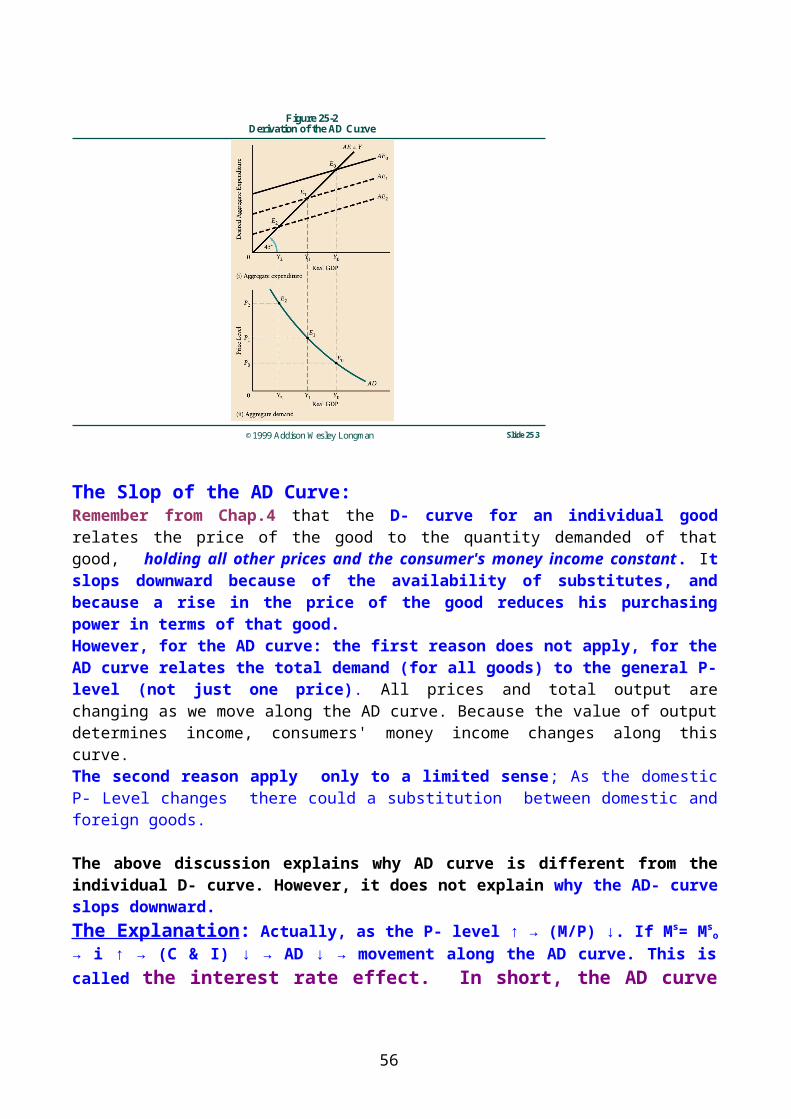
RECALL: The AE curve relates actual GDP to desired AGG.EXPEND. for a given P-Level, plotting GDP on the horizontal axis.The Aggregate Demand Curve (AD) relates equilib. GDP to the price level, again plotting GDP on the horizontal axis. SEE FIG25-2 below. Changes in the P- Level that cause shifts of the AE curve, cause movements along the AD curve. A movement along the AD curve thus traces out the response of quilib. GDP to changes in the price level.
©1999 Addison Wesley Longman Slide 25.3
Figure 25-2Derivation of the AD Curve
The Slop of the AD Curve:Remember from Chap.4 that the D- curve for an individual good relates the price of the good to the quantity demanded of that good, holding all other prices and the consumer's money income constant. It slops downward because of the availability of substitutes, and because a rise in the price of the good reduces his purchasing power in terms of that good.However, for the AD curve: the first reason does not apply, for the AD curve relates the total demand (for all goods) to the general P- level (not just one price). All prices and total output are changing as we move along the AD curve. Because the value of output determines income, consumers' money income changes along this curve.The second reason apply only to a limited sense; As the domestic P- Level changes there could a substitution between domestic and foreign goods.
The above discussion explains why AD curve is different from the individual D- curve. However, it does not explain why the AD- curve slops downward.The Explanation: Actually, as the P- level ↑ → (M/P) ↓. If Ms= Ms
o → i ↑ → (C & I) ↓ → AD ↓ → movement along the AD curve. This is called the interest rate effect. In short, the AD curve slops downward because of the wealth effect and the interest rate effect.
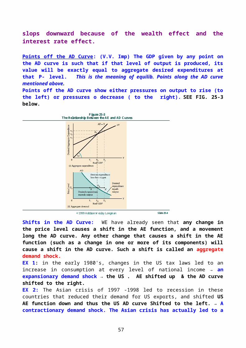
Points off the AD Curve: (V.V. Imp) The GDP given by any point on the AD curve is such that if that level of output is produced, its value will be exactly equal to aggregate desired
44

expenditures at that P- level. This is the meaning of equilib. Points along the AD curve mentioned above.Points off the AD curve show either pressures on output to rise (to the left) or pressures o decrease ( to the right). SEE FIG. 25-3 below.
©1999 Addison Wesley Longman Slide 25.4
Figure 25-3The Relationship Between the AE and AD Curves
Shifts in the AD Curve: WE have already seen that any change in the price level causes a shift in the AE function, and a movement long the AD curve. Any other change that causes a shift in the AE function (such as a change in one or more of its components) will cause a shift in the AD curve. Such a shift is called an aggregate demand shock.EX 1: in the early 1980's, changes in the US tax laws led to an increase in consumption at every level of national income → an expansionary demand shock → the US . AE shifted up & the AD curve shifted to the right.EX 2: The Asian crisis of 1997 -1998 led to recession in these countries that reduced their demand for US exports, and shifted US AE function down and thus the US AD curve Shifted to the left. → A contractionary demand shock. The Asian crisis has actually led to a sharp decrease in oil prices that also generated a prolonged recession in oil exporting countries.
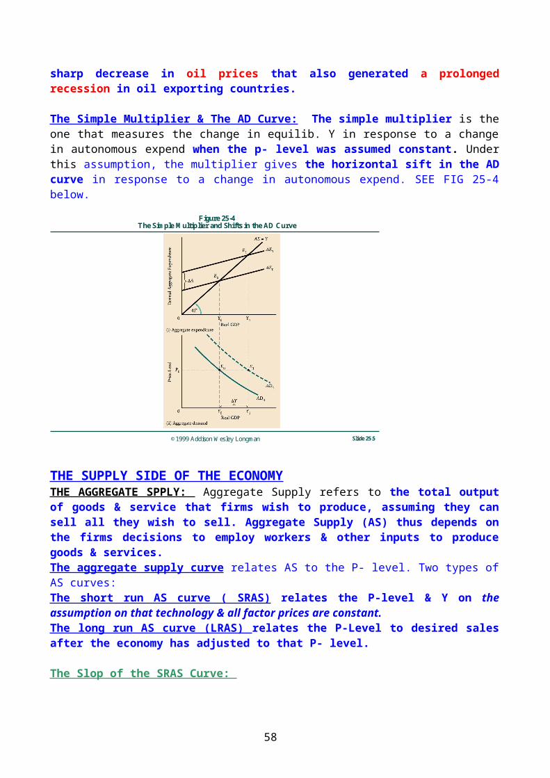
The Simple Multiplier & The AD Curve: The simple multiplier is the one that measures the change in equilib. Y in response to a change in autonomous expend when the p- level was assumed constant. Under this assumption, the multiplier gives the horizontal sift in the AD curve in response to a change in autonomous expend. SEE FIG 25-4 below.
45

©1999 Addison Wesley Longman Slide 25.5
Figure 25-4The Simple Multiplier and Shifts in the AD Curve
THE SUPPLY SIDE OF THE ECONOMYTHE AGGREGATE SPPLY: Aggregate Supply refers to the total output of goods & service that firms wish to produce, assuming they can sell all they wish to sell. Aggregate Supply (AS) thus depends on the firms decisions to employ workers & other inputs to produce goods & services.The aggregate supply curve relates AS to the P- level. Two types of AS curves:The short run AS curve ( SRAS) relates the P-level & Y on the assumption on that technology & all factor prices are constant.The long run AS curve (LRAS) relates the P-Level to desired sales after the economy has adjusted to that P- level.
The Slop of the SRAS Curve:
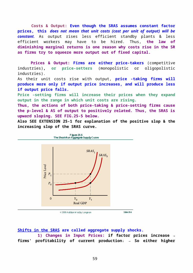
Costs & Output: Even though the SRAS assumes constant factor prices, this does not mean that unit costs (cost per unit of output) will be constant. As output rises less efficient standby plants & less efficient workers may have to be hired. Thus, the law of diminishing marginal returns is one reason why costs rise in the SR as firms try to squeeze more output out of fixed capital. Prices & Output: Firms are either price-takers (competitive industries), or price-setters (monopolistic or oligopolistic industries). As their unit costs rise with output, price -taking firms will produce more only if output price increases, and will produce less if output price falls.Price –setting firms will increase their prices when they expand output in the range in which unit costs are rising.Thus, the actions of both price-taking & price-setting firms cause the p-level & AS of output to positively related. Thus, the SRAS is upward sloping. SEE FIG.25-5 below.Also SEE EXTENSION 25-1 for explanation of the positive slop & the increasing slop of the SRAS curve.
46
©1999 Addison Wesley Longman Slide 25.6
Figure 25-5The Short-Run Aggregate Supply Curve
Shifts in the SRAS are called aggregate supply shocks. 1) Changes in Input Prices: if factor prices increase → firms' profitability of current production↓ → So either higher prices will be required at each output level, or output will be reduced at every price level. SEE Fig. above.An upward shift in the SRAS reflects a reduction in AS due to change in input prices. 2) Changes in Productivity: if labor productivity ↑ → the unit costs of production ( for given wages) ↓ → prices of output ↓. Competing firms cut prices in an attempt to raise their market shares.
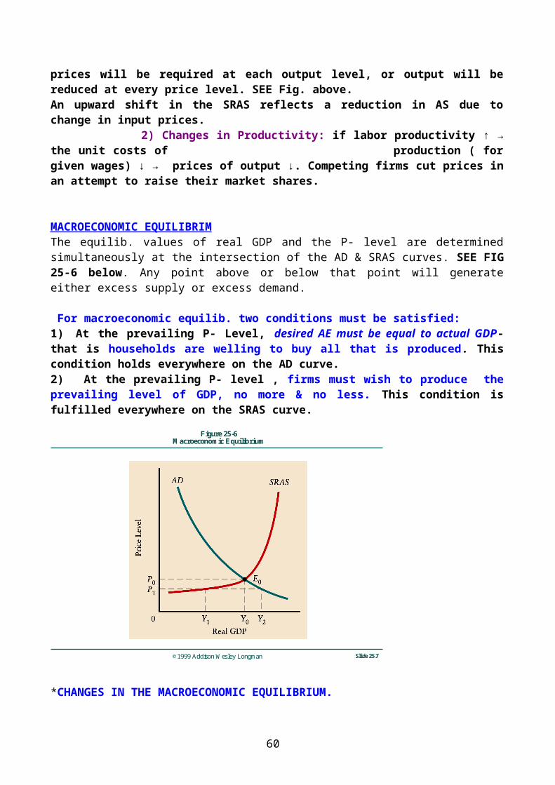
MACROECONOMIC EQUILIBRIMThe equilib. values of real GDP and the P- level are determined simultaneously at the intersection of the AD & SRAS curves. SEE FIG 25-6 below. Any point above or below that point will generate either excess supply or excess demand.
For macroeconomic equilib. two conditions must be satisfied:1) At the prevailing P- Level, desired AE must be equal to actual GDP- that is households are welling to buy all that is produced. This condition holds everywhere on the AD curve.2) At the prevailing P- level , firms must wish to produce the prevailing level of GDP, no more & no less. This condition is fulfilled everywhere on the SRAS curve.
47
©1999 Addison Wesley Longman Slide 25.7
Figure 25-6Macroeconomic Equilibrium
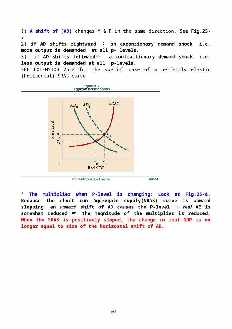
*CHANGES IN THE MACROECONOMIC EQUILIBRIUM.1) A shift of (AD) changes Y & P in the same direction. See Fig.25-72) if AD shifts rightward an expansionary demand shock, i.e. more output is demanded at all p- levels.3) if AD shifts leftward a contractionary demand shock, i.e. less output is demanded at all p-levels.SEE EXTENSION 25-2 for the special case of a perfectly elastic (horizontal) SRAS curve
©1999 Addison Wesley Longman Slide 25.8
Figure 25-7Aggregate Demand Shocks
* The multiplier when P-level is changing: Look at Fig.25-8. Because the short run Aggregate supply(SRAS) curve is upward slopping, an upward shift of AD causes the P-level ↑ real AE
48

is somewhat reduced the magnitude of the multiplier is reduced. When the SRAS is positively sloped, the change in real GDP is no longer equal to size of the horizontal shift of AD.
©1999 Addison Wesley Longman Slide 25.9
Figure 25-8Multiplier When the Price Level Varies
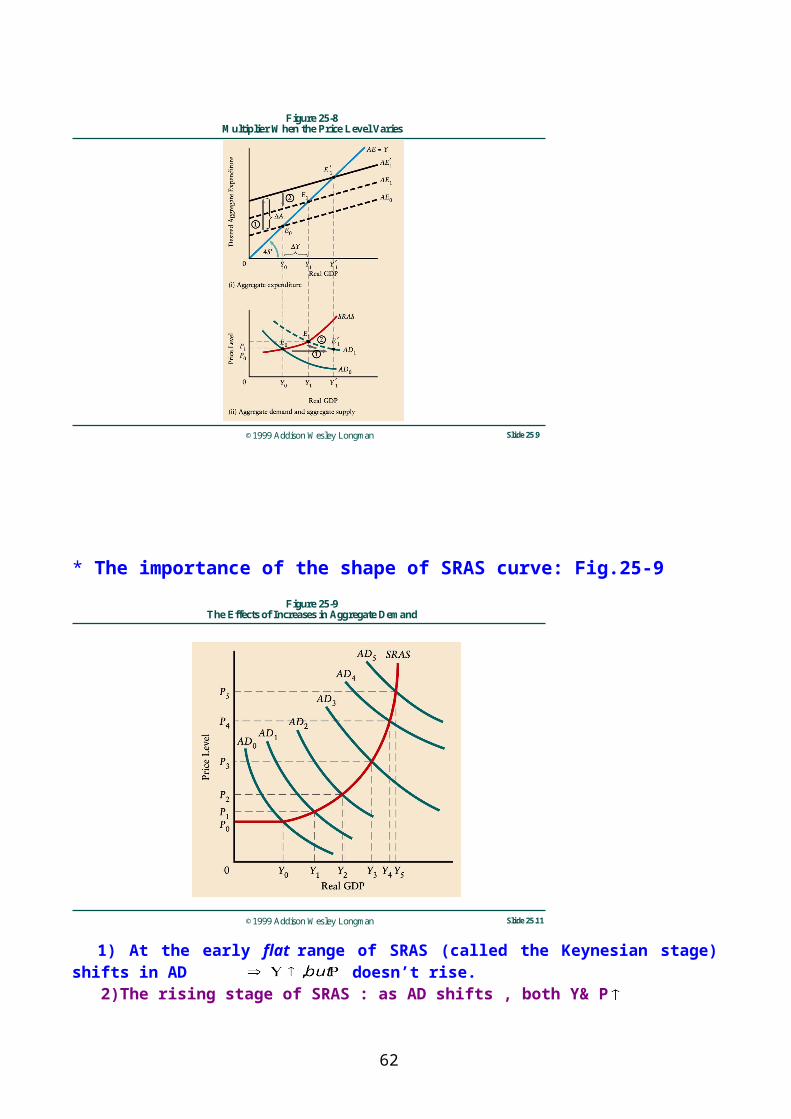
* The importance of the shape of SRAS curve: Fig.25-9
©1999 Addison Wesley Longman Slide 25.11
Figure 25-9The Effects of Increases in Aggregate Demand
1) At the early flat range of SRAS (called the Keynesian stage) shifts in AD doesn’t rise.
49
2)The rising stage of SRAS : as AD shifts , both Y& P 3) The vertical stage, the economy is near full capacity utilization, very little more of output can be added. The shift of AD causes more of P-level rise than output increase. When the SRAS is completely vertical, the economy is at full employment further shifts of AD only causes higher and higher price level, but no more output. See Fig 25-10 below.
©1999 Addison Wesley Longman Slide 25.12
Figure 25-10Demand Shocks When the SRAS Curve is Vertical
However, note that SRAS is used to analyze only short- term effects, for the SRAS assumes constant input prices and technology.
Aggregate supply shocks: Fig. 25-11
©1999 Addison Wesley Longman Slide 25.13
Figure 25-11Aggregate Supply Shocks
50
if inputs prices , profits to firms , for firms to maintain profits, they must charge higher prices at every level of output the short run AS curve shifts up ( to the left) P this is called a case of stagflation “(stagnation +inflation).
Can you remember domestic and international examples of inputs prices increases and how they affected LRAS curves in the respective countries?
END OF CHAPTER 25
Chap.26: Output & Prices in The Long Run* The assumptions from Chapter 25: 1) Inputs prices are constant 2) Productivity is constant.In this chapter we relax the first assumption. We want to see what happens when input prices are variable.Induced Changes in Factor Prices:
51
©1999 Addison Wesley Longman Slide 26.2
Figure 26-1The Output Gap
Since input prices can vary, changes in GDP can induce changes in input prices i) in booms firms are optimistic demand for factors of production . Booms inflationary gaps where Y>Y* & P-level
ii) When firms are pessimistic Profits investment GDP … (opposite to booms)Recession recessionary gap where Y<Y* & P-level Closing the GDP gap: In recessions when demand for factor of production , input prices, especially wages unit cost SRAS shifts rightward until the economy at Y*. In booms: when demand for factors of production input prices, especially wages,unit cost the Short Run Aggregate supply shifts left ward until econ. is at Y*, & P-level .
* Asymmetry in adjustment (V.V. Imp.)As a real -world observation wages are much slower to adjust downward in recession than adjusting upward in booms. Wages are said to be sticky in a downward direction. However, it is not just wages; the international financial and economic crisis that has been going on since 2007 has shown that if business expectations are pessimistic, they may prolong recession that much longer. In addition, the availability of credit (financing) has proven to be very crucial and operates on both the supply side & the demand side of the economy Thus, recession gaps are more difficult to close than inflationary gaps. The economy may take much longer time to get out of recession.
The Philips Curve ( a very Important relation) When real GDP exceeds its potential, an excess demand for labor pushes wages up the unemployment rate is less than U*( the NAIRU) . When real GDP is less than potential, an excess supply is of labor exerts a downward pressure on wages the unemployment rate exceeds U*.This relationship between the unemployment rate, and the rate of change in wages is one of the most famous relationships in macroeconomics & is called the Philips curve.
52
Extension 26-1:The Philips Curve & the Shifting of the SRAS Curve.In the early 1950's professor A.W. Philips, of the London School of Economics pioneered a study on the relationship between the inflation rate and the difference between actual and potential GDP,Y*. Later he studied the relationship between the rate of increase of wages and the level of unemployment. In 1958, he reported that a stable relationship had existed between these two variables for 100 years in the United Kingdom. This relationship came to be known as the Philips Curve. It provided an explanation, rooted in empirical observation, of the speed with which wage changes shifted the SRAS curve by changing unit labor costs. Since unemployment & output gaps are negatively related, we can therefore create another Philips Curve that plots wage changes against output. See the Figure below.Only when Y=Y* is the SRAS not shifting. In this case, AD for labor equals AS; the only unemployment then is frictional and structural. There is then neither upward, downward pressure on wages. Hence the Philips Curve cuts the axis at potential output, Y* and the corresponding level of unemployment is U*.The Philips Curve provided a link between national income models and labor markets. It allowed economists to drop the uncomfortable assumption of sticky money wages.In the figure below, if Y=Y1, the wage cost will be rising to W1. The SRAS will be shifting upward by that amount. Thus, a movement along the Philips Curve, caused by a change in output (and unemployment), implies a change in money wages and thus a shift in the SRAS Curve.What happens if the Philips curve shifts? And what would cause such a shift? an important cause of shifts in the Philips curve is changes in firms' and households' expectations of future inflation.
53
THE EFECTS OF AGGREGATE DEMAND SHOCKS*Expansionary Demand Shocks: See Fig 26-2 below
54

©1999 Addison Wesley Longman Slide 26.3
Figure 26-2The Long-Run Effect of a Positive Aggregate Demand Shock
Suppose equilib. is disturbed by an increase of some autonomous expenditures such as investment. The AD curve shifts upward & GDP rises to y1 > y*, creating an inflationary gap.Closing the Inflationary Gapif Y>Y* unit labor cost - level . Note that prices not to make more profit but to cope with rising costs. However, there is a limit as to how much firms can raise prices because as P-level i.e. demand
Contractionary AD Shocks:
55
©1999 Addison Wesley Longman Slide 26.5
Figure 26-3The Long-Run Effect of a Negative Aggregate Demand Shock
If AD shifts for one reason or another ( Eg. I or X ) Y & becomes < Y* recessionary gap.
Closing the gap Case 1: If wages are flexible. unemployment drives wages shifts to the right until Y= Y*. This is called the automatic (market) adjustment mechanism. i.e the economy reverts back to full employment on its own without any intervention form govt.
Case 2: If wages are not flexible: quite often wages are not flexible and sticky in a downward direction. Unemployment and the recessionary gap may persist for a long period of time if nothing is done about it. So the economy must be activated by some components of AD, usually through govt. stabilization policy. This is an important and very controversial issue of macroeconomics. Fig. 26-3 ii above.
Two important lessons: The asymmetry in wages adjustment helps to explain two facts:
1) Unemployment may persist for a long period of time, without causing wages and unit costs to go down.2) Booms, along with labor shortages and production beyond normal capacity cannot persist for a long period of time, without causing an increase in unit costs and the price level.
Extension 26-2 Anticipated demand shocks:Demand shocks, say by change in Gov't. fiscal policy, if perfectly anticipated by both workers and producers may lead to an equal rise in wages and output prices, such that there will be a simultaneous shift in AD and SRAS curves that leaves real GDP unchanged. In terms of Fig.26-2, the economy may move directly
56
from E0 to E2. Thus, wages and the price level may rise without the presence of an inflationary gap.The possibility that anticipated demand shocks may have no effect on real GDP, plays a key role in some important controversies concerning the effectiveness of Gov't. policy. See Chapters 30 & 31. The scenario explained above requires that everyone have full knowledge of both the exact size of the AD shock & the new equili. values of both wages and prices. Generally, however, people do not have perfect knowledge & foresight, so there are some temporary real GDP effects until the final equilib. of wages and prices is reached.
Demand Shocks & Business Cycles:
Each component of AD is subject to continual random shifts which are sometimes large enough to disturb the economy significantly. Adjustment lags convert such shifts into cyclical fluctuations in Y. The time needed for the economy to adjust depends on the source and magnitude of the shock. It should be noted that using AD to activate the economy may also take time to bring results. Activating existing plants, hiring and training workers takes time. The multiplier process that translates an initial increase in autonomous expenditures to income takes time. However, AD policies are usually faster to work than the automatic adjustment mechanism.
The Long Run Aggregate Supply Curve ( LRAS): is AS curve when the economy has fully adjusted to all shocks. There is no excess demand, nor excess supply in any market. It is vertical at potential GDP. This is sometimes called “The classical AS curve”, because classical economists were more inserted in the long run.SEE Fig 26-4 below
57
©1999 Addison Wesley Longman Slide 26.6
Figure 26-4Long-Run Equilibrium and Aggregate Supply
If the economy is already at long run position i.e. Y=Y*, further shifts in AD only causes price level . The LRAS is consistent with any price level. However, output may be pushed beyond its LR position only if the economy’s capital stock and/or its technology rise. This means that potential GDP (Y*) rises. This implies that LRAS shifts to the right.
LR Equilibrium: The Composition of output in The LR:
If the economy is already at LR Equilib., a shift in AD because of G and/or I (P & W) SRAS curve P - level (C & NX) (AE= AE & Y=Y*) a rise in autonomous G & I crowds out C & NX => The composition of national output changes. There will be more of public & investment goods but less of consumption and exportable goods. The position of LRAS is determined by past economic growth.
Three ways for GDP to change:
58
©1999 Addison Wesley Longman Slide 26.7
Figure 26-5Three Ways that Real GDP Can Increase
1) Increases in AD: if AD shifts, a recessionary gap can be closed. A further shift turns the recessionary gap into on inflationary one. unit cost closing the gap at a higher price level.2) Temporary increase in AS: If there is a temporary increase in AS decrease in input prices shifts downward unit cost . This will have no effect on LRAS and Y*. However if input prices swing up again, the cycle is reversed.3) Permanent Increase in AS: If the productive capacity of the economy increases, potential GDP increases LRAS shifts to the right.* Sources of LR Econ. Growth (Very Imp.)1) Governance of the law and equal opportunities 2) Improvement in labor productivity through education and training. 3) Changes in labor laws that reduce rigidities in the labor market. 4) Capital accumulation. 5) Population growth and natural discoveries. 6) Technological breakthroughs.
* Sources of cyclical changes in GDP ( Very Imp.) Changes in interest rates, exchange rates, govt. policy, input prices, change in consumer and producers confidence.
SEE FIGURE 26-6 below for three different economic series.
59
©1999 Addison Wesley Longman Slide 26.8
Figure 26-6Fluctuations in Economic Activity, 1960-1997
* The Basic Theory of Fiscal Stabilization: FIG.26-7 & 8The basic power of fiscal policy is our knowledge about which direction it should take. However, there are problems with knowing the right timing, magnitude and mixture. *Using fiscal policy to eliminate a recessionary gap:Fig26-7
©1999 Addison Wesley Longman Slide 26.9
Figure 26-7The Closing of a Recessionary Gap
a) If we rely on market automatic adjustment mechanism, shifts to the right but it could take time. b) Using fiscal policy (G , or T ,or both) AD shifts . This method shortens the period required to close the gap, but it could take place at the same time when private decision makers are increasing their expenditures. The AD curve may shift too much to the right creating an inflationary gap.
60
* Using Fiscal Policy to eliminate an Inflationary gap: Fig 26-8: An opposite reasoning to the one above.
©1999 Addison Wesley Longman Slide 26.10
Figure 26-8The Closing of an Inflationary Gap
* A Key Proposition: when the automatic adjustment mechanism fails to operate quickly enough, there is room for stabilizing fiscal policy. This has been the way countries dealing with the recession resulting from the international financial crisis (2007- ); mainly through injecting government money into the financial and real sectors of the economies, in addition to lowering the interest rates (Using monetary policy.)
* The Paradox of Thrift: states that an increase in savings at the individual level can be good, but it may be bad if it is widespread in the whole economy. A rise in S . The policy implication of the paradox of thrift is that in case of recession the govt. should indulge in budget deficit i.e. should have G>T, not the other way aroundLimitation: It works as long as Y<Y* only. When Y=Y*, a rise in AE & AD only rises the P-level. In the LR, economic growth is determined by the position of LRAS.
* Automatic stabilizers:Even in the absence of active fiscal policy, the existence of taxes and transfer payments act as automatic stabilizers to the economy. T –G = tY-G. In case of recession, as Y .This reduces leakages from the economy, puts a partial break to the downward shift of AD. Also, during recession, transfer payments (like unemployment insurance & social security) , slowing AD shift. In the case of a booming economy, the opposite is true. Tax revenues are said procyclical (They go up in booms & go down in recessions.)Limitations of Discretionary Fiscal Policy 1)Lags: a) Decision lags: changes in fiscal policy may require the approval of different govt. organizations. Also, whose taxes and how much should they be changed? What expend. Should be increased or decreased?
61
b) Execution lags: time between a decision taken and implementation. The economic consequences may take some time to be felt. It is possible that by the time a given policy decision has any impact on the economy, the behavior of the private sector may shift the AD curve too far, converting a recessionary gap into an inflationary one. SEE FIG. 26-9 below.
©1999 Addison Wesley Longman Slide 26.11
Figure 26-9Effects of Fiscal Policies That Are Not Reversed
2) Temporary vs. Permanent Policy Changes: Temporary tax measures are generally less effective than measures that are expected to be permanent. If households feel that tax cuts are to last for short periods, they will adjust their consumption very little.
The Role of Discretionary Fiscal Policy:Fine Tuning: Trying to use economic policy to remove or to offset all fluctuations in private -sector spending to hold GDP near its potential at all times. However, the above – mentioned difficulties must be remembered.Gross Tuning: Many economists still argue that when the recessionary gap is large and persistent, occasional (gross) tuning must be used.FISCAL POLICY AND GROWTH (V.V.Imp):The desirability of using fiscal policy to stabilize the economy depends upon:a) The speed of the economy's own adjustment mechanism.b) in an economy that is at or near its potential level, expansive FP may lower national saving and national asset formation and consequently lowers future economic growth. HOWEVER, THIS IS A VERY CONTROVERSIAL ISSUE. It depends on how and where government is spending. SEE CHAPTER 32 on "GOVERNMENT DEBT & DEFICITS".
END OF CHAPTER 26
Chapter 27: The Nature of Money & Monetary Institutions
What is Money?* Money is a generally accepted medium of exchange.
62
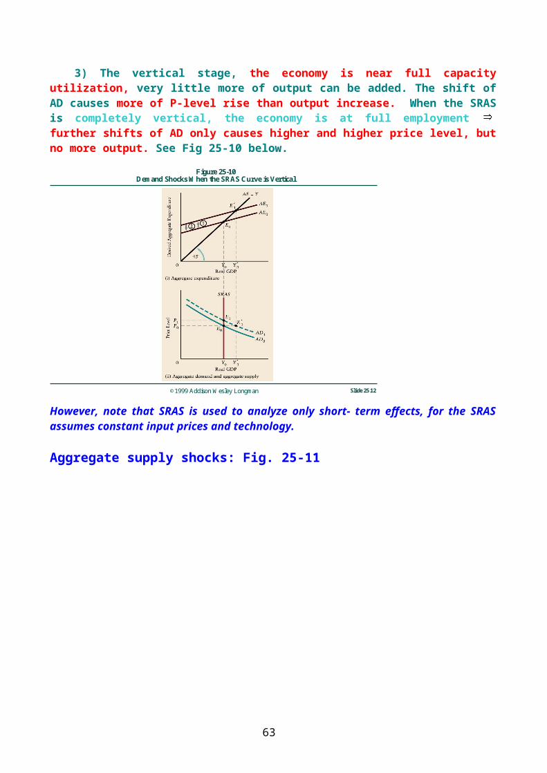
* Functions of money:-1) A medium for exchange2) A store of value3) A standard of measurement of value4) A means for deferred payments (debts)
THEORITICAL PERSPECTIVES ON MONEY
THE CLASSICAL VIEW: Economists of the eighteenth & nineteenth centuries claimed that potential GDP(Y*) is independent from monetary factors. They distinguished sharply between the "real sector" and the "monetary sector" of the economy. This is now referred o as the Classical dichotomy.According to this view:1) The allocation of resources, and hence the determination of real GDP, is determined only by the real sector of the economy.2) It is relative prices, including the level of wages relative to the price of commodities, that matter for this process.3) The price level is determined in the monetary sector of the economy. i.e the p- Level is determined by the rate of growth of MS.4) If the quantity of money were doubled, other things being equal, the prices of all commodities and money (nominal) income would double. Relative prices would remain unchanged, & the real sector of the economy would be unaffected.5) The doctrine that the quantity of money influences the level of money prices but has no effect on the real part of the economy is called the neutrality of money. Money is spoken of as a "veil" behind which occur the real events that affect material well-being.
THE MODERN VIEW: 1) most modern economists accept the insights of the Classical economists that relative prices are the major determinant of the allocation of resources, and that the quantity of money has a lot to do with determining the absolute level of prices.2) They accept the neutrality of money in the LR when all forces causing change have fully worked themselves out.3) However, they do not accept the neutrality of money when the economy is adjusting to the forces that caused it to change- that is when the economy is not in a state of LR equilibrium.4) Consequently, they reject the Classical dichotomy of the economy in the SR.5) The LR neutrality of money makes modern economists stress the strong link between money & the P- Level, especially over long periods of time.
Figure27-1 below gives long run perspective on prices in the USA. Two things stand out from the figure. First, there has been periods of dramatic price reductions. Second, there has been more or less uninterrupted increase in the P- level – positive inflation rates- since the end of World War II.
63

©1999 Addison Wesley Longman Slide 27.2
Figure 27-1An Index of Producer Prices in the United States
1785-1997 (1967 = 100)
* How do commercial banks affect money supply in the economy.?* Assumptions:1)Money supply is currency plus demand deposits at banks.2) There is only one type of assets: (loans), only one type of liabilities: (demand deposits). Liabilities generate costs, assets generate revenues.3) Banks hold a fixed ratio of cash and reserves to deposits. E.g. 20%. 4) No cash drain form banks households keep a fixed amount of cash with them. See Tables 27-3 -10 below. This is extremely Important * Accounting identity: Assets = Equity + Liabilities.
TABLE 27-3The Initial Balance Sheet of Incidental
Bank and Trust (IB&T)
Assets = Equities + Liabilities Cash and other reserves 200 Deposits 1,000Loans 900 Capital 100
1,100 1,100
IB&T has a reserve of 20 percent of its deposit liabilities. The commercial bank earns money by finding profitable investments for much of the money deposited with it. In this balance sheet, loans are its earning assets.In table 27-3 above* Amount of loans= (Equities + liabilities) - cash and reserves
* final change in deposits (for the whole banking system). in reserves in Res , where 1/ is the money multiplier ________________ = __________ required reserve ratio
64
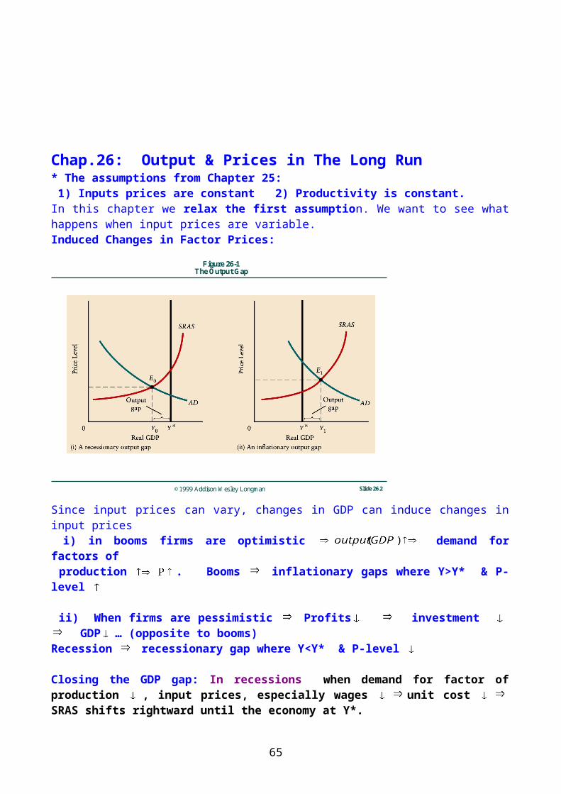
= 100 = 100 = (100)(5)= 500. In this case the money multiplier =5 0.2 2/10
* The assumption of no cash drain implies: in money supply = in deposits
The change of money supply by commercial banks is not an automatic process. It depends on 1) risk perceived by banks and
2) expected change in future interest rates. 3) The preferences of banks and households all have an impact on money supply in the economy.
TABLE 27-4IB&T's Balance Sheet Immediately
After a New Deposit of $100
Assets Liabilities Cash and other reserves 300 Deposits 1,100Loans 900 Capital 100___________________ 1200 1200The deposit raises deposit liabilities and cash assets by the same amount. Because both cash and deposits rise by $100, the bank's actual reserve ratio, formerly 0.20, increases to 0.27. The bank has more cash than it needs to provide a 20 percent reserve against its deposit liabilities.
TABLE 27-5IB&T's Balance Sheet After a New Loan
and Cash Drain of S80
Assets Liabilities_______________________________________________________Cash and other reserves 220 Deposits 1,100Loans 980 Capital 100
1200 1,200 * in loans = in deposits - in reserves IB&T lends its surplus cash and suffers a cash drain. The bank keeps $20 as a reserve against the initial new deposit of $100. It lends $80 to a customer, who writes a check to someone who deals with another bank. When the check is cleared, IB&T suffers an $80 cash drain. Comparing Tables 27-3 and 27-5 shows that the bank has increased its deposit liabilities by the $100 initially deposited and has increased its assets by $20 of cash reserves and $80 of new loans. It has also restored its required reserve ratio of 0.20.
TABLE 27-6Changes in the Balance Sheets of
Second-Generation Banks
Assets Liabilities
65
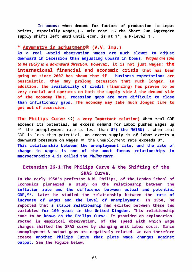
Cash and other reserves 16 Deposits +80Loans + 64 ______________________________________________________ +80 +80Second-generation banks receive cash deposits and expand loans. The second-generation banks gain new deposits of $80 as a result of the loan granted by IB&T, which is used to make payments to customers of the second-generation banks. These banks keep 20 percent of the cash that they acquire as their required reserve against the new deposit, and they can make new loans using the other 80 percent. When the customers who borrowed the money make payments to the customers of third-generation banks, a cash drain occurs.
TABLE 27-7The Sequence of Loans and DepositAfter a Single New Deposit of $100
Addition to New New
Bank, Deposits Loans Reserves
IB&T $100.00 $80.00 $20.002nd-generation bank 80.00 64.00 16.003rd-generation bank 64.00 51.20 12.804th-generation bank 51.20 40.96 10.24Sth-generation bank 40.96 32.77 8.196th-generation bank 32.77 26.22 6.557th-generation bank 26.22 20.98 5.24Sth-generation bank 20.98 16.78 4.209th-generation bank 16.78 13.42 3.36lOth-generation bank 13.42 10.74 2.68________________________________________________________________Total for first 10 generations 446.33 357.07 89.26All remaining generations 53.67 42.93 10.74Total for banking system 500.00 400.00 100.00
The banking system as a whole can create deposit money whenever it receives new deposits. The table shows the process of the creation of deposit money on the assumptions that all the loans made by one set of banks end up as deposits in another set of banks {the next-generation banks), that the required reserve ratio {v) is 0.20, and that banks always lend out any excess reserves. Although each bank suffers a cash drain whenever it grants a new loan, the system as a whole does not, and in a series of steps it increases deposit money by l/v, which, in this example, is five times the amount of any increase in reserves that it obtains.
TABLE 27-8Change in the Combined Balance Sheetsof All the Banks in the System Following
The Multiple Expansion of Deposits
66
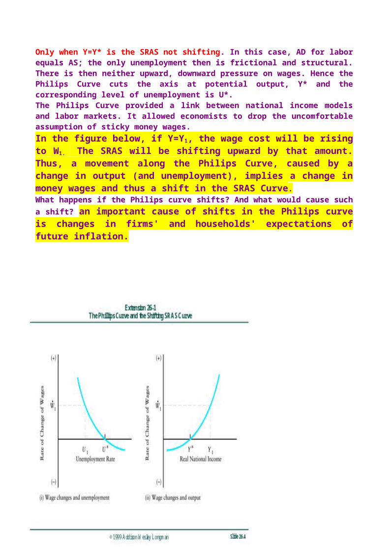
Assets Liabilities_________________________________________________________Cash and other reserves +100 Deposits +500Loans +400_________________________________________________________
+500 +500
The reserve ratio is returned to 0.20. The entire initial deposit of $100 ends up as reserves of the banking system. Therefore, deposits rise by (1/0.2) times the initial deposit-that is, by $500.
TABLE 27-9Change in the Combined Balance Sheets of All the Banks
in the System Following the Multiple Expansionof Deposits with a Cash Drain of $20
Assets Liabilities_______________________________________________________________Cash and other reserves +80 Deposits +400Loans +320_______________________________________________________________
+400 +400
The reserve ratio is 0.20, and cash drain is 0.05. Only $80 of the initial deposit of $100 ends up as reserves of the banking system. Deposits therefore rise by (1/0.2) times the $80-that is, by $400. The cash drain ($20) is 5 percent of the increase in deposits ($400).
Note: Change in Deposits= (1/(1/5) ) ( Change in Res.) = (5) (80)= 400 Change in Loans = Change in Dep. – Change in Res.= 400- 80= 320
THE MONEY SUPPLY : The total stock of money in the economy at any moment is called the money supply or the supply of money. Economists use alternative definitions of MS.
Definitions of Money Supply: See table 27-10 below. M1 concentrates on the medium- of- exchange function of money. M2 & M3 contain assets that serve the temporary store- of – value function and are in practice quickly convertible into a medium of exchange.
TABLE 27-10Money Supply in the United States, November 1997 " I
(billions of dollars)
Currency 421.9Demand deposits 391.0
67

Traveler's checks 8.2Other checkable deposits 243.0
M1 1,064.1
Money market mutual fund balances 590.4Money market deposit accounts andsavings deposits 1,380.2Small-denomination time deposits 963.2
M2 3,997.9
Large-denomination time deposits 573.4Term repurchase agreements 2 33.5Term Eurodollars 133.9Institutional money marketmutual funds 346.4M3 5,285.1
The three widely used measures of the money supply are M1, M2, and M3. The narrow definition of the money supply concentrates on what can be used directly as a medium of exchange. The broader definitions add in deposits that serve the store-of-value function and can be readily converted to a medium of exchange.Note that M1 includes traveler's checks held by the public, which are clearly a medium of exchange. Within M3, repurchase agreements are funds lent out on the overnight money market, and Eurodollars are U.S. dollar-denominated deposits in U.S. banks located outside the United States. M2 and M3 include similar items, with the difference in most cases being that the term deposits are in MJ and the demand deposits in M2.(Source: Economic Report of the President, 1998.)
Students should look at SAMA Annual Reports for definition and measures of monetary aggregates in Saudi Arabia.
http://www.sama.gov.sa NEAR MONEY & MONEY SUBSTITUTES: An important debate of monetary policy centers on what is the appropriate definition of money. The problem arises because some assets perform poorly as a store- of –value, while others perform poorly as a medium- of – exchange. For example during times of inflation, currency (or M1 assets in general) may well serve as a medium- of exchange , but poorly as a store of value. In contrast, heavy gold bars (& M2 and M3 assets) may do the opposite. Assets that fulfill adequately the store- of – value function and are readily convertible into a medium of exchange, but are not themselves medium of exchange (such as M2 & M3) are sometimes called near money. Usually M1 assets do not earn any income, while M2 & M3 do. Why would anyone hold M1 assets? It is because of the transaction costs (the cost of inconvenience in this case) involved in converting assets back and forth from one account into another.
68
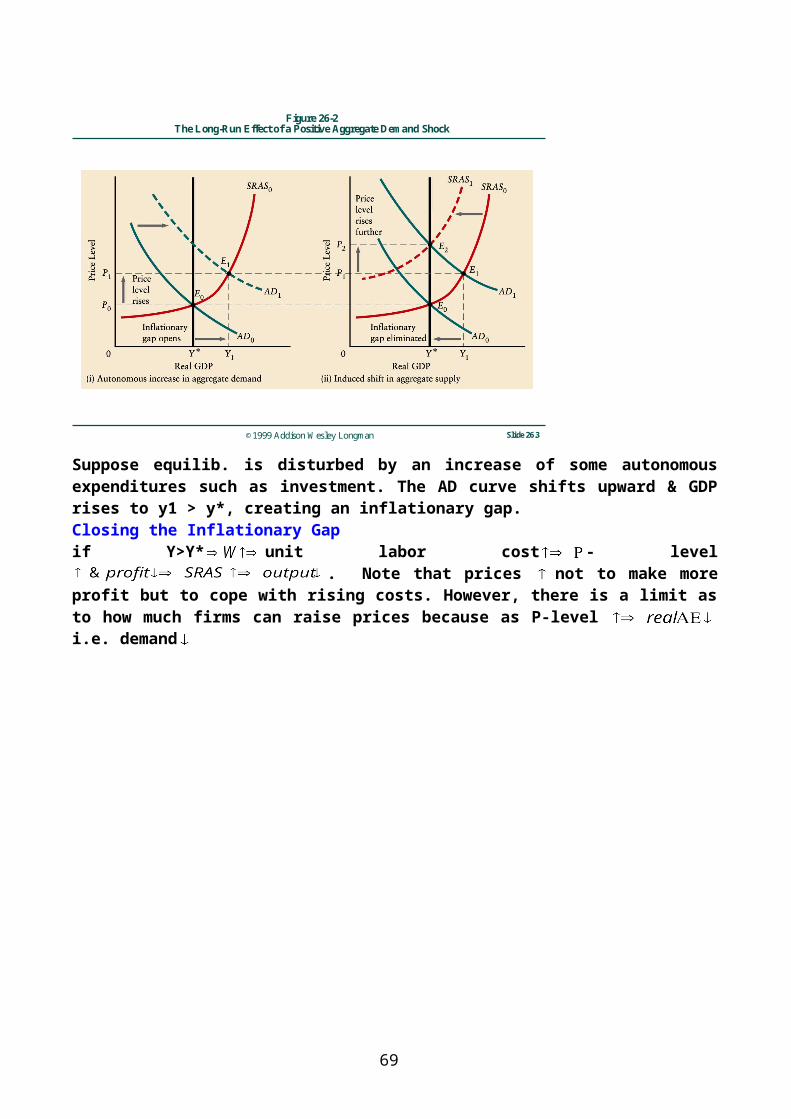
Things that serve as temporary media of exchange but are not a store of value are sometimes called money substitutes. Credit cards are a prime example.
CHOOSING A MEASURE: The definition of money supply for the purpose of conducting monetary policy has been debated among economists at least as early as the eighteenth century. The specifics of the definition will continue to change over time as new monetary assets are developed to serve some if not all the functions of money. For the purpose of this course, we will focus on the medium- of – exchange function of money and hence money will be currency plus deposits that can be withdrawn and converted on a very short notice.
Question1: What is the difference between total stock of money and GDP?Question2: How do we classify ATM cards? Are they near monies or money substitutes?
END OF CHAPTER 27
Chapter 28: MONEY, OUTPUT, & PRICES
The relationship between the interest rate & the price of a bond: If i↑→ Pb ↓ & vise versa why?Suppose i = 5% per year & the price of a bond, Pb= SR100. At the end of the year, the investor has SR 105. if i↓ to 3% how much does the investor need to invest in order to get SR105? Answer: he needs to invest more than 100 → as i ↓, Pb ↑ and visa versa.
For simplicity, we assume that (wealth) is only Money balances + Bonds.
In a capitalist economy, the interest rate represents the opportunity cost of holding money. What is the opportunity cost of holding money in an Islamic economy? Q: If there is an opportunity cost to holding money, why do people hold money?
The motives for the demand for money (Why Do People Hold Money?):- 1) The Transaction Motive: payments & receipts are rarely synchronized. Thus, people & firms need to hold money to conduct their transactions. The size of the transaction demand for money is affected by the size and no. of transactions, which is affected by level of income (GDP) . MTr = f (Y+).2) The Precautionary Motive: To cover the holders of money against emergency situations when payments are suddenly > receipts. The amount held for those purposes is a function of the cost of borrowing & the level of income. MPr = f (i-, y+ ). 3) The Speculative Motive: This was first discussed by John Maynard Keynes & later explained further by James Tobin, the1981 Noble Laureate in Economics. This demand for money is driven by speculative expectations about future interest rates & the prices of stocks and bonds. MSP= f(i-). Because their prices fluctuate, stocks and bonds are risky assets. Many H.H & firms are risk averse. Investors must balance the expected interest or profit from bonds
69
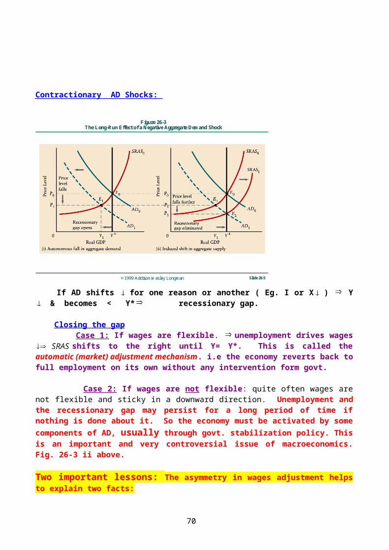
and stocks against the risk of price fluctuations. Thus, they try to diversify their holdings between money and financial assets.
REAL & NOMINAL MONEY BALANCES:Real values are measured in purchasing power units; nominal values are measured in money units. The real demand for money is the nominal quantity divided by the price level: md = Md/ P. If increases in nominal money balances are matched by a rise in the P- Level, the increase in real balances is that much reduced. Demand for real money balances is determined by real GDP (Y) & i.
However, the nominal demand for money, Md = f ( p+, y+, i-). So if y & i are held constant, a rise in P increases Md proportionately. Note: the three motives are not "visible" in reality, but each is partially responsible for the total demand for money. See FIG 28-1 below.The relationship between i & Md is called the liquidity preference function (LP).
©1999 Addison Wesley Longman Slide 28.2
Figure 28-1The Demand for Money as a Function of Interest Rates, Income, and the Price Level
Monetary Equilib. & Aggregate Demand
The liquidity Preference (Portfolio Balance) Theory of the Interest Rate (A Keynesian Theory of what determines the interest rate): Monetary equilib. occurs when the supply and demand for money are equal. In the money market, the interest rate is the "price" that adjusts to bring about equilib. The LP theory implies that the interest rate is determined in the monetary, rather than the real sector of the economy, (contrary to the neo-classical belief.)
70

©1999 Addison Wesley Longman Slide 28.3
Figure 28-2The Liquidity Preference Theory of Interest
If, for some reason, the economy is at i1 → ED for money. How does the Mkt adjust? ED for money→ people sell some bonds → Pb↓ → i↑→ the opp. cost of holding money ↑→ demand for money ↓ (moving upward along LP-Function) until the economy rests at i0. Alternatively: if i=i2 , → ES: The scenario is reversed. The Transmission Mechanism: The mechanism by which disturbances in the monetary (financial) sector are transmitted to the real sector.It goes in 3 stages. 1) Disturbance of Md & Ms affects the interest rate.2) From the interest rate to Investment & AE3) From AE into AD & GDP
See Fig28-3 ,-4 -5 & -6Monetary equilib. can be disturbed either because of a change in money supply or money demand. See Fig.28-3.
©1999 Addison Wesley Longman Slide 28.4
Figure 28-3Monetary Disturbances and Interest Rate Changes
71
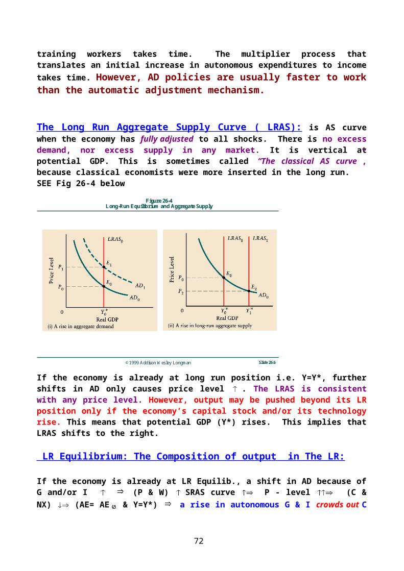
©1999 Addison Wesley Longman Slide 28.5
Figure 28-4The Effects of Changes in the Money Supply on Investment Expenditure
©1999 Addison Wesley Longman Slide 28.6
Figure 28-5The Effects of Changes in the Money Supply on Aggregate Demand
72

©1999 Addison Wesley Longman Slide 28.7
Figure 28-6Transmission Mechanism for an Expansionary Monetary Shock
The transmission mechanism shows the very important role of the interest rate in “regulating” the capitalist economy. It affects both the monetary & real sectors of the economy.
AGG . DEMAND & AGG .Supply: A rise in money supply causes AD to shift upward, but because the price level may rise (SRAS is upward sloping), the increase in real GDP is less than the horizontal shift of AD. SEE Fig 28-7 below.
©1999 Addison Wesley Longman Slide 28.8
Figure 28-7The Effects of Changes in the Money Supply
73
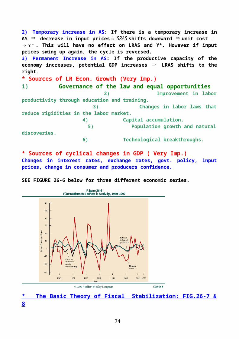
A Further look at the slope of the AD:-In previous chapters, we explained the downward slope of AD on the basis of:a) The wealth effect:As P-level ↑→real wealth ↓→ AE↓→ AD↓b) The substitution effect: as P-level ↑→ people substitute foreign goods for domestic goods → AE ↓ →AD ↓c) Now the interest rate effect: if P-level ↑→Md ↑, if Ms=Ms
0 (i.e. central
bank does not increase MS) → i ↑ → (I &C )↓ →AD↓This link is very important because it is known empirically that the interest rate is the most important link between the monetary sector & real expenditure flows.
More on The Automatic Adjustment Mechanism: a) The rise in the demand for factors of production →their prices↑→ profits ↓ →firms reduce output & employment of factors of production →SRAS shifts upward. b) As AD ↑→ P ↑→ i↑ ( provided MS is constant) →I↓→ AE↓, AD↓(a movement along the AD).
Thus, the interest rate effect reinforces the automatic adjustment mechanism to close a GDP gap in the economy.. Note that (a) above, operates on the supply side of the market and (b) operates on the demand side of the market. An Important Proposition: A sufficiently large increase in the P-level will eventually eliminate any inflationary gap, provided there is no further increase in money supply.
Frustration of The Adjustment Mechanism:Q: what happens if the central bank continues to increase MS? See fig. 28-8 below.
74
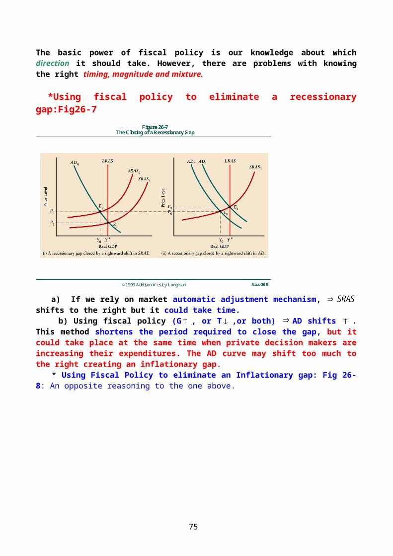
©1999 Addison Wesley Longman Slide 28.9
Figure 28-8Frustration of the Adjustment Mechanism
An Expansionary Monetary Policy → AD0 → AD1→ inflationary gap (y↑ &P↑). If this is a once - and –for- all increase in Ms → the automatic adjustment mechanism will close the gap → SRAS shifts upward. However, if the central bank continues its expansionary monetary policy, the automatic adjustment mech. is frustrated, AD shifts to AD2, GDP stays at Y0. However, P↑↑. Inflation is said to be validated.
The Strength (effectiveness) of the Monetary Policy(V.V.Imp.): Fig.28-9 below shows that the adjustment mechanism operates to insure that in the LR, regardless of the rate of growth of the money supply, real GDP converges to its potential level. This is often referred to as the long run neutrality of money. In other words, in the long run changes in the rate of growth of money supply cannot influence potential real GDP. This is a much- debated issue.
©1999 Addison Wesley Longman Slide 28.10
Figure 28-9The Long-Run Neutrality of Money
Short Run Effects Of Money Supply: Two views on The Strength of Monetary policy. See Fig 28-10 ( V.V. Imp.)
75
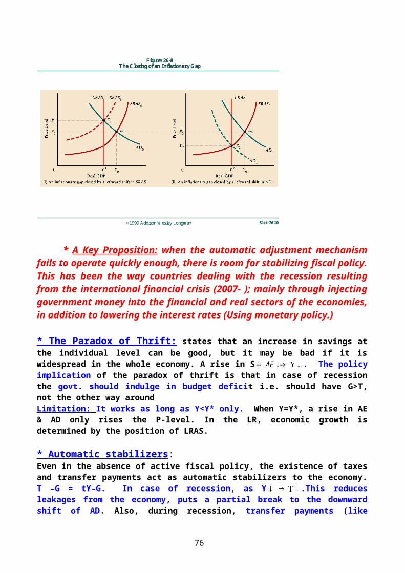
©1999 Addison Wesley Longman Slide 28.11
Figure 28-10Two Views on the Strength of Monetary Changes
Effective Monetary Policy Requires Two Conditions:1) a relatively inelastic function of the demand for money (LP has relatively sharp slope)2) a relatively elastic demand for investment. (MEI slope is relatively small).What does each condition mean?The monetarists' view is that monetary policy is effective (the upper panel of the figure.)The lower panel represents the Keynesian view that monetary policy is ineffective. The Keynesian alternative to activate the economy would be fiscal policy.
END of Chapter 28
76
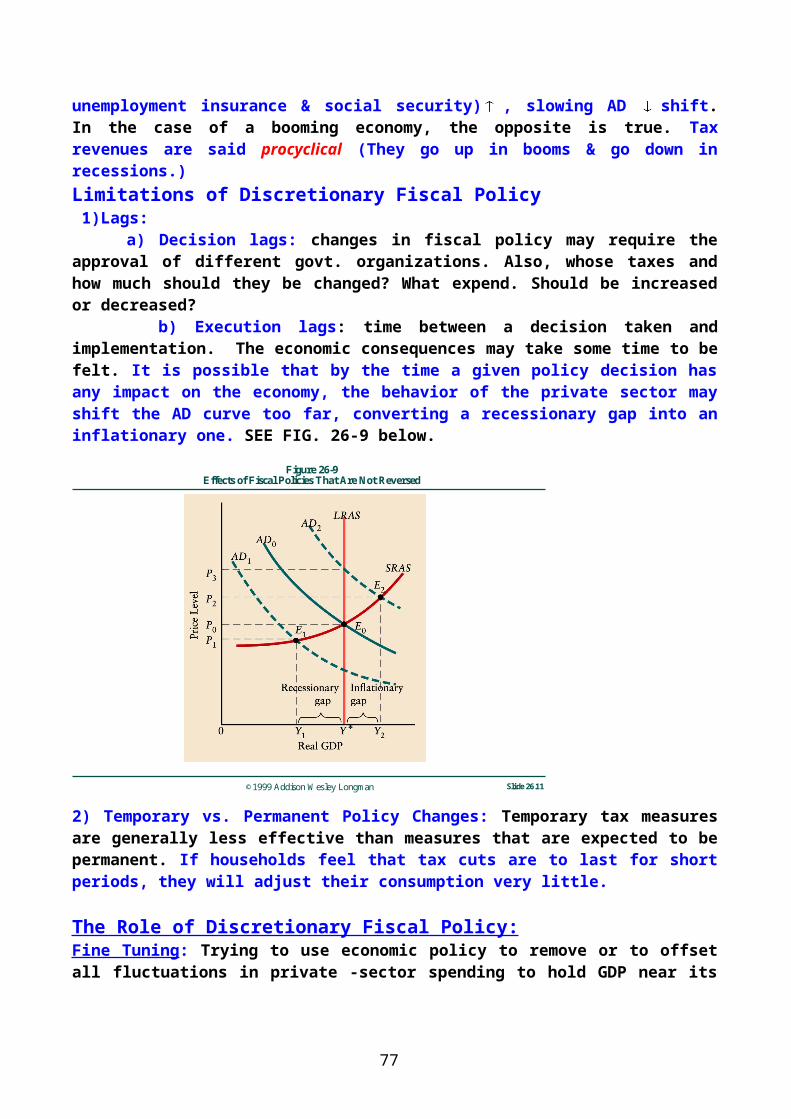
Chapter 29: Monetary Policy
I) Policy Instruments: - are tools in the hands of the Central Bank to conduct Monetary Policy. These are:1) Open Market Operations (OMO): The central bank buying & selling govt. securities (bonds).If the C.B. would like to increase money supply, the C. B. buys govt. securities from individuals, firms, or the gov't. and gives them money in return. It issues a check against itself. The check holder deposits it in his bank account → Deposits at banks ↑→ The Bank deposits the check in its acct. at the CB.→ Bank reserves (or the monetary base= C +R)↑→ the bank's ability to extend loans & accept deposits ↑. To reduce Money Supply, the C.B. sells govt. securities. See table 29.1
2) Required Reserves Ratio (RRR ): assuming banks are loaned up (no excess reserves). If the CB increases the RRR, banks must reduce deposits. This is done by:a) not extending new loansb) calling back some old loans →deposits at Banks ↓ →MS ↓ The impact on MS of increasing RRR is definite i.e it reduces money supply. However, if the Central Bank decreases RRR→ Banks will have more reserves →Banks can, but do not have to extend more loans and accept more deposits. The impact on MS of reducing RRR is not definite. It depends upon Banks' decisions to lend, and decisions of H.H. and Firms to borrow.
3) The Discount Rate:- is the interest rate at which the Central Bank lends to commercial banks to meet short terms shortages of reserves. The CB is said to be a lender of last resort. The operation is conducted through the discount window. The discount rate as a cost of borrowing, affects directly interest rates charged by commercial banks. It is called the discount rate because for banks to borrow from the CB, they sell some of their holdings of government bonds to the CB at a discount of the face value.
77
Policy Instruments:OMO, RRR, DR, CREDIT CONTROLS
Intermediate TargetsMs, i, ER
Policy VariablesGDP(y), P - level (P) & Unemp (u)
In Saudi Arabia, the discount rate (when banks borrow from SAMA) is called the "Repo". When banks have excess liquidity and deposit additional reserves with SAMA, they get an interest rate called "Reverse Repo." 4) Credit Controls: like maximum interest rates on consumer loans, mortgage rates, margin requirements…. Etc. Check SAMA and CBB (Central Bank of Bahrain) web cites for consumer credit controls. A Review of The Transmission Mechanism:
II) Policy Variables & Policy Instruments : The CB policy variables (The variables that it would like to influence) are real GDP, the P-Level, & unemployment. Monetary policy shifts the AD curve and changes P & Y simultaneously. Therefore, the CB cannot control both independently. If it targets one, it must accept the consequences for the other. For this reason, the CB often, but not always, concentrates on nominal GDP, (PY) as a target in the SR. See the article at the end of the chapter.
Monetary policy and LRSA: It is argued by some economists (called monetarists) that in LR, monetary policy have no impact on LRAS, and thus in LR monetary policy can only influence the P-level. This is called the principle of the neutrality of money. This is a highly controversial issue. The alleged LR neutrality of money (that money cannot affect LR GDP) led many CB's to concentrate on the inflation rate as the LR target of monetary policy. The European Central Bank (ECB) is an example. The first Chairman of the ECB, Wilhelm Duisenberg said in the inaugural speech of the ECB (January 1999) "Monetary policy is neither the cause, nor the cure of unemployment." This means that the prime policy variable for the ECB has been price level stability (i.e. fighting inflation). Consequently, the charter of the ECB does not allow it to purchase government bonds, and thus is not supposed to participate in financing budget deficits of the member governments. Governments are supposed to float bonds in the market. This has changed a little bit, however, with the current financial crisis, since 2007, as the ECB has been participating in stabilizing European economies, and purchased large amounts governments' bonds.III) Intermediate Targets: i, MS, & ERDaily information about policy variables(Y,P,&U) are rarely available. Hence, policy makers typically use intermediate targets indicated above. To serve as a target, a variable must satisfy two criteria. First, information about it must be available on frequent basis-
78
daily if possible. Second, its movements must be closely correlated with those of the policy variable. Since the C.B. can not effect directly the policy variables (Y,P,U) it tries to influence what is called intermediate target (the Ms or i). These are not independent from each other, targeting one automatically determines the other. See Fig,29-2 belowIt may sound immaterial which variable to target. In reality, they are not the same.
©1999 Addison Wesley Longman Slide 29.3
Figure 29-2Alternative Intermediate Targets
Debate about Intermediate TargetsTargeting the Interest Rate:-Monetarists argue that the interest rate is pro-cyclical (i.e. it rises in booms, & decreases in recessions). Thus, it is hard to tell whether the interest rate is changing due to the phase of the business cycle or due to C.B Policy. Monetarist Prefer the C.B. concentration on monetary aggregates (the growth rate of money supply), in particular on M1. The Keynesian Counter Argument:- 1) Targeting money supply is a reasonable policy only if the function of the demand for money is stable. In many cases, it is not. In the figure 29-3 below, the C.B. fights inflationary pressures by reducing MS (so that i ↑). However, if L.P. function isn’t stable and for some reason LP↓, i ↓ instead of rising, 2) Also, which monetary aggregate to target? Suppose CB targets M1. If there is change in households preferences from demand deposits into saving deposits → M1↓ & M2↑. The CB may have to change its target accordingly.
Most central banks today concentrate on the interest rate as their intermediate target.
79

©1999 Addison Wesley Longman Slide 29.4
Figure 29-3Intermediate Targets When the Demand for Money Shifts
The Role of Exchange Rate:-
Changes in the ER can affect X &M →affect AE & AD→(Y&P)Two sources of change in ER:-a) If X↑→ demand for the country's currency ↑→ ER↓(currency appreciates)→ (AE=AD) ↑→P↑ in other words, the sources of change in ER is in this case is a rise in demand for exports. The CB may try to curb inflation by trying to restrain the economy close to its potential.( Does this sound a wise policy ?) b) The other case:- suppose there is a rise in the demand for the country’s financial assets (stocks & bonds )→demand for currency of the country ↑→ ER↓ (currency appreciates) → (X ↓ & M ↑ )→ AD ↓ →P↓. The C.B may try to stimulate the economy by trying to keep GDP close to its potential
Conclusion:Movements in the ER can provide valuable information for the conduct of monetary policy. The two cases above show that although in both cases the ER appreciates, yet the source of change could have very different impact on the conduct of monetary policy and the economy.
LAGS IN THE CONDUCT OF MONETARY POLICY
A Historical Debate (See Application 29-1): Monetarists believe that monetary policy is very powerful in affecting the economy in the SR. Keynesians believe otherwise. The source of debate goes at least as early as the great depression, which was accompanied,( may have been started), by bank failures →MS↓→AD↓
The counter argument was that the great depression in Canada & UK wasn’t accompanied by bank failures, so there wasn’t reduction in MS.
The debate involved more than just the size of the effect of change in MS. It focused on factors that are thought to render monetary policy ineffective. The debate centered on lags & uncertainty:
80
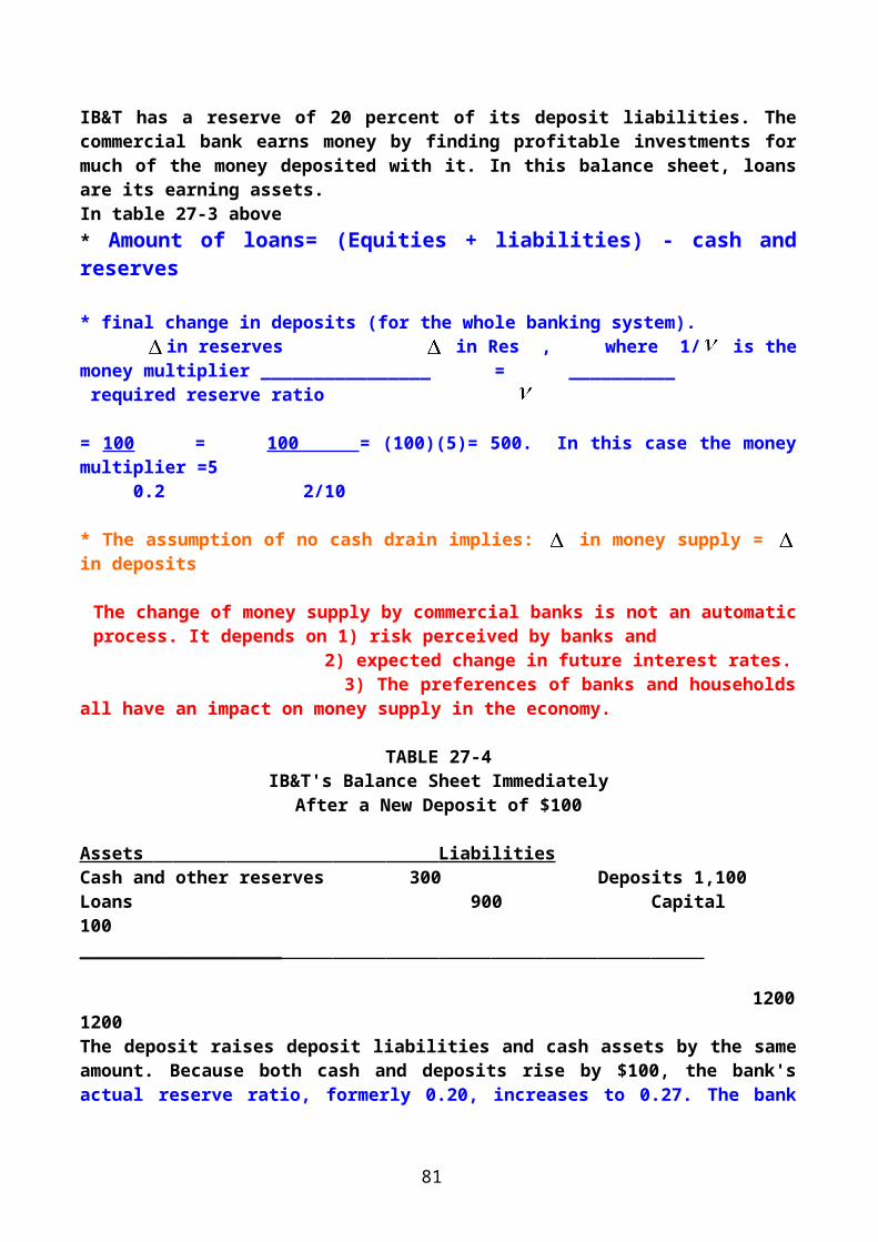
Sources of execution lags in monetary policy: monetary policy may not be effective because of execution lags due to
(1) lags in creation and destruction of demand deposits: it depends upon decisions by both commercial banks, households and businesses.
(2) Investment plans take time to be decided upon & implemented
(3) The full multiplier effect takes time to show its impact on the economy.
The long & variable execution lags makes monetary fine tuning difficult & may be destabilizing to the economy.
A MONETARY RULE:
Monetarists believe that:
monetary policy is a potent (effective) force of expansionary & contractionary pressures;
1) Monetary policy works with long & variable lags;
2) The CB may indulge in sudden & sharp reversals in its policies.
Monetarists believe that the CB should stop stabilizing the economy. Instead, it should expand MS, year in and year out at a constant rate that is equal to the rate of growth of real GDP. When the rate of growth shows signs of long-term change, the CB adjusts the rate of money expansion.
Many other economists disagree with the monetarists and believe that fine tuning of MS can in principle reduce cyclical fluctuations.
The possibility of an unstable function of the demand for money, explained earlier, is mentioned as a major counter argument. In this case, a constant –money rule may be destabilizing.
LESSONS FOR MONETARY POLICY:
Inflation & Monetary Growth: Does an increase in the rate of money growth rate necessarily cause a rise in the inflation rate? The relationship is not so tight to be viewed as automatic or mechanical, nor does it appear to resolve the issue of causality. In other words,
is it as MS ↑ → P-level ↑ ? Or is it that
as the P-level ↑ , MS has to rise ?
Historical experience shows that there is an unmistakable connection between MS & the P- level. Monetarists believe in the first line of causality. Others believe money expansion was mainly a passive reaction to price increases caused by aggregate supply shocks.
An important lesson : a sharp reduction in monetary growth led to high interest rates, a sever recession, and a dramatic reduction in inflation in the USA in the early 1980s.
81
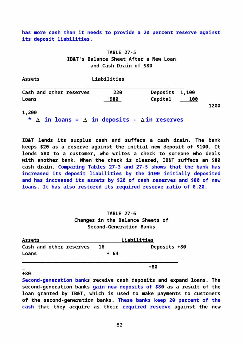
The experience of the 1990's shows that in the presence of AD shocks, GDP growth and inflation are positively related. In the presence of AS shocks, GDP growth and inflation are negatively related. The growth of the American (and other western) economies in the late 1990's can be explained by the following AS shock events:
a) The collapse of the Southeast Asian economies that began in 1997-1998 led to a reduction in those countries' demand for raw materials. The reduction in world input prices implied a positive AS shock to western economies.
b) Also, as the currencies of Asian countries depreciated, the cost of imports from these counties declined, thus reinforcing the Positive AS shock to western economies.
c) The collapse of the USSR ( the former Soviet Union) in the early 1990s enabled the USA to reduce military spending & relieved resources for civilian use.
The Stock Market: How would a negative shock to the stock mkt. (such as the crash of October 19, 1978 in the USA) affect the economy & monetary policy? How was a crisis avoided? A fall in stock prices coupled with rising interest rates was expected to slow economic expansion. The crash had a smaller effect on the American economy than expected. This was largely due to strong infusion of liquidity by the Fed into the American economy.
How would a positive shock to the stock mkt . (Such as that of 1994-1998) affect the economy & monetary policy? A rise in prices of bonds implies wealth of H.H rise, which in turn implies consumption rises. The American economy was already heating up. Because of the height of the stock market (Dow Jones reached 9000 points) a crash was expected. This would have decreased H.H wealth significantly & reduce AD.
What was the impact of the crash of he Saudi Stock Market in May 2004 and the Big Stock market Crash of February, 2006? How different was it from the US case?
CONCLUSIONS:
1) The economy is too complex for simple monetary rule to provide the best monetary policy.
2) Monetary policy can vary between being restrictive & expansive for reasons that are related to shifts in the private sector's demand for money, and not necessarily related to change in CB policy.
3) To judge the stance (position) of current monetary policy, the CB needs to monitor a number of variables.
4) Contrary to what was once believed, monetary policy is a very potent tool for influencing AD. It may be difficult, however to predict how fast & how strongly a given policy will operate, but if the CB is prepared enough, it can reduce inflation.
5) There is room for debate about whether the result is worth the cost (in terms of GDP).
END OF CHAPTER 29
82
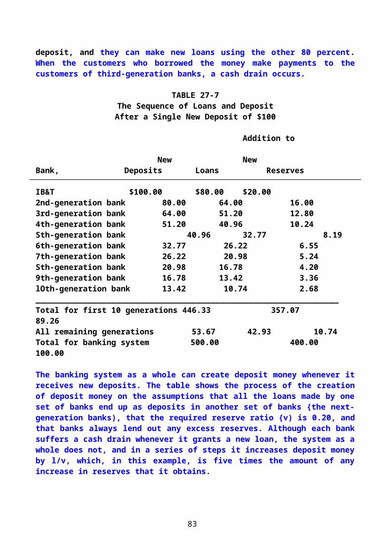
Print Jeffrey Frankel
Jeffrey Frankel, a professor at Harvard University's Kennedy School of Government, previously served as a member of President Bill Clinton’s Council of Economic Advisers. He directs the Program in International Finance and Macroeconomics at the US National Bureau of Economic Research, where he is a member of the Business Cycle Dating Committee, the official US arbiter of recession and recovery.
The Death of Inflation Targeting
16 May 2012
CAMBRIDGE – It is with regret that we announce the death of inflation targeting. The monetary-policy regime, known as IT to friends, evidently passed away in September 2008. The lack of an official announcement until now attests to the esteem in which it was held, its usefulness as an ornament of credibility for central banks, and fears that there might be no good candidates to succeed it as the preferred anchor for monetary policy.
Inflation targeting was born in New Zealand in March 1990. Admired for its transparency, and thus for facilitating accountability, it achieved success there, and soon in Canada, Australia, the United Kingdom, Sweden, and Israel. It subsequently became popular in Latin America (Brazil, Chile, Mexico, Colombia, and Peru) and among other developing countries (including South Africa, South Korea, Indonesia, Thailand, and Turkey).
One reason that IT gained such wide acceptance as the monetary-policy anchor of choice was the demise of its predecessor, exchange-rate targeting, in the currency crises of the 1990’s. Pegged exchange rates had come under fatal speculative attack in many of these countries, whose authorities thus needed something new to anchor the public’s expectations concerning monetary policy. Inflation targeting was in the right place at the right time.
In the early 1980’s, prior to the reign of exchange-rate targeting, the fashion was money-supply targeting, the brainchild of the monetarist Milton Friedman. But that rule succumbed rather quickly to violent money-demand shocks, though Friedman’s general argument – that a credible commitment to low inflation requires favoring rules over discretion – remains very influential.
Inflation targeting was best known as a rule that instructed central banks to set – and try their best to attain – a target range for the annual rate of change of the consumer price index (CPI). Close cousins included targeting the price level instead of the inflation rate, and targeting core inflation (the CPI minus volatile food and energy prices).
There were also proponents of flexible inflation targeting , who held that it was fine to put some weight on real GDP growth in the short run, so long as there was a clear longer-term target for CPI inflation. But some felt that if the definition of IT were stretched too far, it would lose its meaning.
83
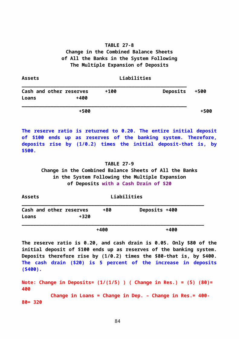
Regardless of the form it took, IT began to receive some heavy blows a few years ago (analogous to the crises that hit exchange-rate targets in the 1990’s). Perhaps the biggest setback hit in September 2008, when it became clear that central banks that had been relying on IT had not paid enough attention to asset-price bubbles.
Central bankers had told themselves that they were giving asset markets all of the attention that they deserved, by specifying that housing prices and equity prices could be taken into account to the extent that they implied information regarding goods inflation. But this escape clause proved insufficient: when the global financial crisis hit (suggesting, at least in retrospect, that monetary policy had been too loose from 2003 to 2006), it was neither preceded nor followed by an upsurge in inflation.
That the boom-bust cycle could occur without inflation should not have come as a surprise. After all, the same thing happened when asset-price bubbles ended in crashes in the United States in 1929, Japan in 1990, and Thailand and Korea in 1997. And the hope of long-time US Federal Reserve Chairman Alan Greenspan that monetary easing could clean up the mess in the aftermath of such a crash proved wrong.
While the lack of response to asset bubbles was probably IT’s biggest failing, another major setback was inappropriate responses to supply shocks and terms-of-trade shocks. An economy is healthier if monetary policy responds to an increase in the world prices of its exported commodities by tightening enough to cause the currency to appreciate. But CPI targeting instead tells the central bank to tighten policy in response to an increase in the world price of imported commodities – exactly the opposite of accommodating the adverse shift in the terms of trade.
It is widely suspected, for example, that the reason for the European Central Bank’s otherwise puzzling decision to raise interest rates in July 2008, as the world was sliding into the worst recession since the 1930’s, was that oil prices were just then reaching an all-time high. Oil prices are given substantial weight in the CPI, so stabilizing the CPI when dollar-denominated oil prices go up requires euro appreciation vis-à-vis the dollar.
One candidate to succeed IT as the preferred nominal monetary-policy anchor has lately received some enthusiastic support in the economic blogosphere: nominal GDP targeting. The idea is not new. It had been a candidate to succeed money-supply targeting in the 1980’s, since it did not share the latter’s vulnerability to so-called velocity shocks.
Nominal GDP targeting was not adopted then, but now it is back. Its fans point out that, unlike IT, it would not cause excessive tightening in response to adverse supply shocks. Nominal GDP targeting stabilizes demand – the most that can be asked of monetary policy. An adverse supply shock is automatically divided equally between inflation and real GDP, which is pretty much what a central bank with discretion would do anyway.
A dark-horse candidate is product-price targeting, which would focus on stabilizing an index of producer prices rather than an index of consumer prices. Unlike IT, it would not dictate a perverse response to terms-of-trade shocks.
Supporters of both nominal GDP targeting and product-price targeting claim that IT sometimes gave the public the misleading impression that it would stabilize the cost of living, even in the face of supply shocks or terms-of trade-shocks, over which it had no control.
84
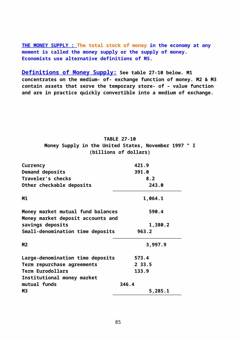
Inflation targeting is survived by the gold standard, an elderly distant relative. Although some eccentrics favor a return to gold as the monetary anchor, most would prefer to leave this relic of another age to its peaceful retirement.
This article is available online at:http://www.project-syndicate.org/commentary/the-death-of-inflation-targeting
Copyright Project Syndicate - www.project-syndicate.org
85

CHAPTER 31: UNEMPLOYMENT
Remember from Chap. 21:The unemployed are people who are without jobs and are actively searching for jobs.In macroeconomics, economists distinguish between the NAIRU, and the rate of cyclical unemployment, which is unemployment associated with fluctuations of real GDP around its potential (Y*). Issues of this chapter: 1) Cyclical unemployment, why it exists and why the adjustment mechanism often takes so long to make it disappear. 2)Unemployment rate follows a cyclical path, rising during periods of recession and falling in periods of business expansion. What are the sources of these cyclical fluctuations? What are the sources of the upward trend?
3) Are government policies partly (and perhaps unintentionally) responsible for increases in the NAIRU? Can government policy do anything to reduce the NAIRU?
Changes in the Total Employmen t:
On the supply side, the causes have included a rising population, increased labor force participation by various groups, especially women; and net immigration of working-age persons.
On the demand side, economic growth causes some sectors of the economy to decline and others to expand. Recessions are a major cause of unemployment.
SEE SAMA's ANNUAL REPORT FOR DATA ON SAUDI EMPLOYMENT & LABOR FORCE
http://www.sama.gov.sa
Flows in the Labor MarketUsually the focus on the labor market tends to be on the overall level of employment and unemployment rather than on the amount of job creation and job destruction. This focus can often lead us to the conclusion that few changes are occurring in the labor market when in fact the truth is exactly the opposite. The disaggregation of data may reflect a very active labor market with very large amounts of both gross job creation and gross job destruction. The size of change in either or both areas reflects the degree of dynamism in the economy. Economists & policy makers must look at both gross & net flows in the labor market.
SEE APPLICATION 31-1Consequences of Unemployment : Two costs of unemployment. 1)Lost Output. According to an empirical relation sometimes called Okun’s Law-named after the economist Arthur Okun (1928-1980), for every percentage point of unemployment above the NAIRU, output falls by about 2.5 percentage points below potential output. This loss represents a serious waste of resources.
86
2)Personal Costs. The loss of self-esteem and the dislocation of families that often result from situations of prolonged unemployment are genuine tragedies, in addition to rising crime.Classification of UnemploymentThe unemployed can be classified by personal characteristics, such as age, sex, degree of skill or education, or ethnic group. They can also be classified by geographical location, occupation, duration of unemployment, or reasons for unemployment.The recorded figures, for unemployment may significantly understate or overstate the numbers of people who are actually willing to work at the existing wages. Overstatement arises because the measured figure for unemployment includes people who are genuinely not interested in work but say they are interested in order to collect unemployment benefits.( Some people registered in Hafiz Program may be an example.) Understatement arises because of people who would like to work but have ceased to believe that suitable jobs are available for them, voluntarily withdraw form the labor force. Although these people are not measured in the survey of unemployment (which requires that people actively look for work), they are unemployed in the sense that they would accept a job if one were available at going wage rates. People in this category are referred to as discouraged workers.
Three types of unemployment: Cyclical, frictional, and structural. Both frictional and structural unemployment exist even when real GDP is at its potential level, and hence there is neither a recessionary gap nor an inflationary gap.
Cyclical Unemployment: a) The term cyclical unemployment refers to unemployment that occurs whenever real GDP is below potential GDP. b) People who are cyclically unemployed are normally presumed to be suffering involuntary unemployment in that they are willing to work at the going wage rate.c) It can be measured by the difference between the No. of people currently employed & the No. of people who would be employed at potential output.d) The fluctuations in aggregate demand cause real output to fluctuate around its potential level. f) If all of the labor markets had fully flexible wage rates, wages would fluctuate to keep quantity demanded in each individual market equal to the quantity supplied in that market. Employment and the labor force would be pro-cyclical rising in booms and falling in slumps), but there would be no significant amounts of involuntary unemployment. Some people would withdraw from the labor force, being unwilling to work at the lower wage. The case of flexible (competitive) labor markets is shown in FIG. 31-1 – part(i) blow.
87
©1999 Addison Wesley Longman Slide 31.3
Figure 31-1Employment and Wages in a Competitive Labor Market
The realities of the world are however different. Although wages do tend to vary over the cycle, the fluctuations are not sufficient to remove all cyclical unemployment. Why is this so? Two types of explanation have been advanced in recent years.
New Classical TheoriesThe classical theory assumes that labor markets are always in equilibrium in the sense that the quantity demand is continually equated with quantity supplied. If not, it gives two explanations for unemployment:
a)Fluctuation in the willingness of people to supply their labor. The supply of labor increases in booms, and falls in recessions. This explanation of cyclical behavior in the labor market has two problems. First, wages will tend to rise in slumps and fall in booms, which is not what we observe. SEE FIG 31-1, part(ii) above. Second, there will still be no systematic cyclical unemployment because labor markets always clear, leaving everyone who wished to work actually working. Supply-induced fluctuations in employment form part of the basis of what is called real business cycle (RBC) theory, which is discussed in Extension 31-1.
b) Second line of explanation lies in errors on the part of workers and employees in predicting the course of the price level over the business cycle. In chapter 28, we saw that the increase in the money supply leads to an increase in desired aggregate expenditure and a rise in prices of both inputs & outputs. Firms will produce more and workers will work more since both groups think they are getting an increased relative price for what they sell. Thus total output and employment rise. The extra output and employment occur only while people are being fooled. When both groups realize that their relative prices are in fact unchanged, output & employment will fall back to their initial levels. The only difference is that now the price level is higher, leaving relative prices unchanged. New Classical explanations assume that labor markets clear, and then they look for reasons why employment fluctuates. They imply, therefore, that people who are not
88
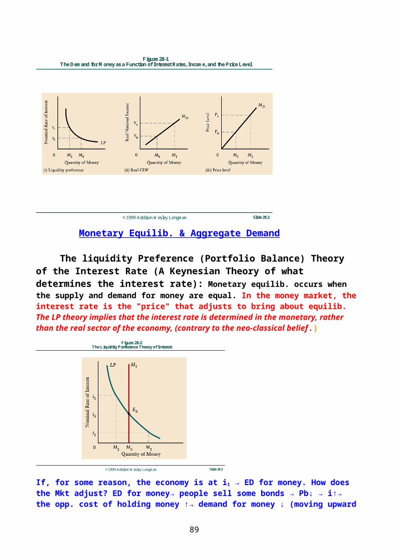
working have voluntarily withdrawn from the labor market for one reason or another; there is no involuntary unemployment.
New Keynesian TheoriesKeynesian economists believe that:a) People correctly read mkt. signals, but react in ways that do not cause markets to clear at all times . b) Many people are involuntarily unemployed in the sense they would accept an offer for jobs they are trained for, at the going mkt. wage rate, if such an offer were made.c) These theories start with the everyday observation that wage rates do not change every time demand or supply shifts. SEE FIG. 31-2 below.
©1999 Addison Wesley Longman Slide 31.4
Figure 31-2Unemployment with Sticky Wages
TWO KENESIAN EXPLANATIONS:
I) Long Term Employment Relationships Both workers and employers look for relatively long-term and stable employment relationships. Workers want job security in the face of fluctuating demand. Employers want workers who understand the firm’s organization, production, and marketing plans. Wages are not the only determinant of employment decisions, & they become insensitive to fluctuations in current economic conditions. Given this situation, the tendency is that employers “smooth out” the income of employees by paying a steady money wage and letting profits and employment fluctuate to absorb the effects of temporary increases and decreases in demand for the firm’s product.
Many long-term contracts provide for a schedule of money wages over a period of several years. Similarly, fringe benefits, such as pensions and health care, tend to bind workers to particular employers. Another example is payment that rises with years of service. This helps to bind the employee to the company, whereas seniority rules for layoffs bind the employer to the long-term worker.
89
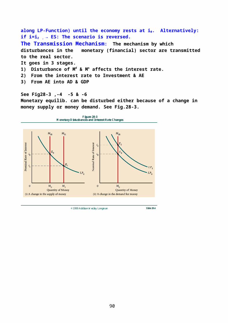
Thus, in labor markets in which long-term relationships are important (and this is the case in many labor markets), the wage rate does not fluctuate to continuously clear the market. Wages are written over what has been called the long term “economic climate” rather than the short-term “economic weather”. Because wages are thus insulated from short-term fluctuations in demand, any market clearing that occurs does so through fluctuations in the volume of employment rather than in wages. Of course, wages must respond to permanent shifts in mkt. conditions.
II) Efficiency Wages
Employers may find that workers may become more efficient if they are paid somewhat more than the minimum amount to induce workers to work for them. This increases the opportunity cost to workers if they shrink on the job & get fired.Several economists observed that, workers who feel that they are treated well, work harder than those who believe that they are treated badly. This gives a reason for paying an efficiency wage, provided that the increased output from treating workers well covers the increased cost of doing so. A variant of efficiency wage theory seeks to explain why firms do not cut wages during recessions. If workers feel unfairly treated when their wages are reduced, wage reductions (at least in response to moderate recessions) may cost firms more (in lost output from unhappy employees) than they save in reduced wages. If so, real wages may not fall rapidly enough to eliminate involuntary unemployment.The basic message of New Keynesian theories of unemployment is that competitive labor markets cannot be relied upon to eliminate unemployment by equating current demand for labor with current supply. As a result, unemployment will rise and fall as the demand for labor rises and falls over the cycle.THE NAIRU is composed of frictional and structural unemployment. Our interest is in how the NAIRU changes over time and in the extent that economic policy can affect the NAIRU.
FRICTIONAL UNEMPLOYMENT
Frictional unemployment results from the normal turnover of labor. An important source of frictional unemployment is young people who enter the labor force and look for jobs. Another source is people who leave their jobs because they are dissatisfied or fired. Persons who are unemployed while searching for jobs are said to be frictionally unemployed or in search unemployment.
How “voluntarily” is frictional unemployment? Some of it is clearly voluntary. An extreme New Classical view regards all frictional unemployment as voluntary. Critics of that view argue that many frictionally unemployed workers are involuntarily unemployed because they lost their jobs through no fault of their own (e.g. their factories may have closed down) and have not yet located specific jobs for which they believe they are qualified. The distinction between voluntary and involuntary unemployment is not always clear, as it might at first seem. SEE EXTENSION 31-2
90
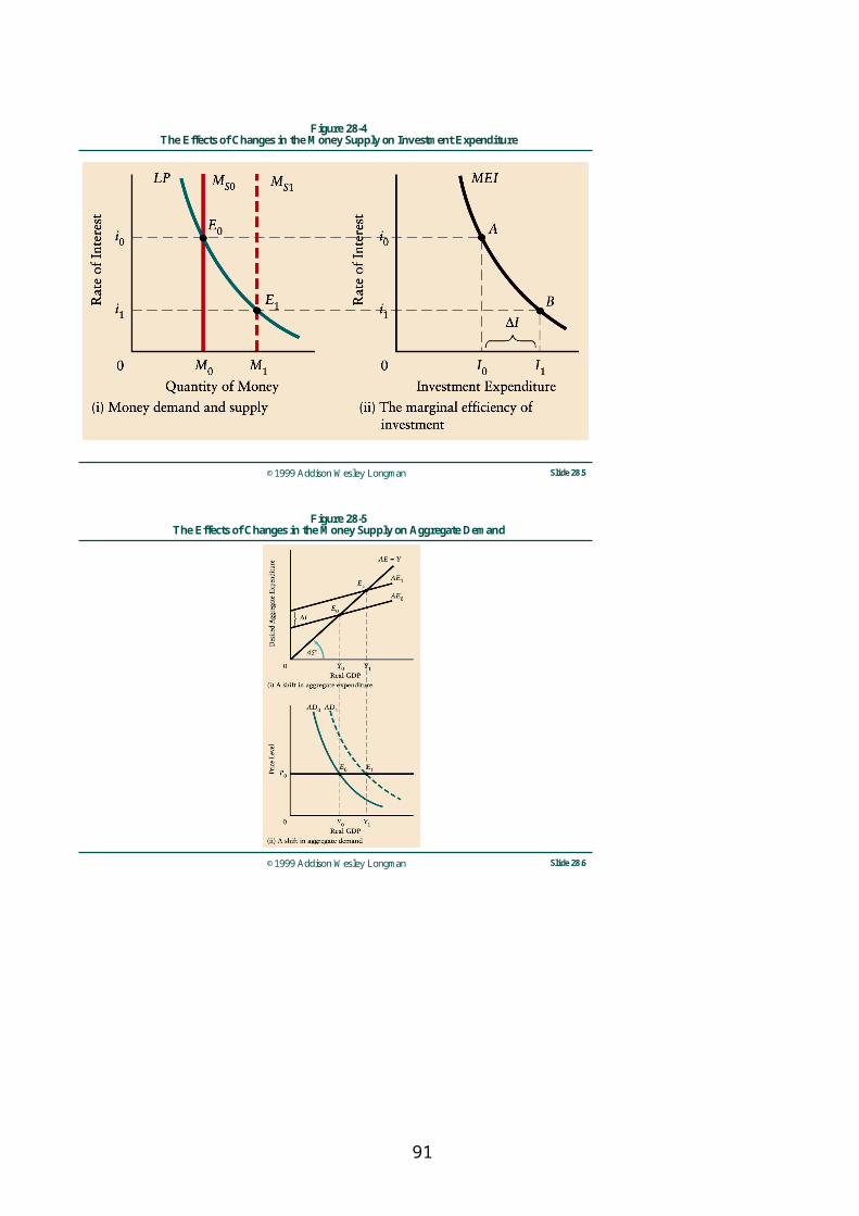
STRUCTURAL UNEMPLOYMENT
Structural adjustments in the economy can cause unemployment. When the pattern of demand for goods and services changes, the pattern of the demand for labor changes too. Such unemployment may be defined as unemployment caused by a mismatch between the structure of the labor force in terms of skills, occupations, industries, or geographical locations – and the structure of the demand for labor.
1) Natural Causesa) Changes that accompany economic growth shift the structure of the demand for labor, especially if it generates a significant shift toward high-skilled jobs. The evolutionary shift toward service-sector employment and the restructuring within all industries in response to technological change has favored workers with more years of schooling. Some existing workers can retrain and some new entrants can acquire fresh skills, but the transition is often difficult, especially for already experienced workers whose skills become economically obsolete. b) Increases in international competition can also cause structural unemployment. This could happen either through the immigration of industries to other countries, or through the increase imports of cheaper products.
2) Policy Causesa) Policies that discourage firms from replacing labor with machines may protect employment over the short term. However if the industry cannot compete effectively, an industry decline may cause more unemployment in the LR.b) Minimum wage laws can cause structural unemployment by pricing low-skilled labor out of the market. This is a very controversial issue. c) Unemployment Insurance. In some countries, unemployed workers are generally eligible for unemployment insurance only if they have worked for a given number of weeks in the previous year-this is known as the entrance requirement. In some cases these ER are very low & encourage seasonal workers to work for a few months & collect UI. See www.hafiz.gov.sa www.mol.gov.sa for conditions of unemployment benefits in Saudi Arabia. d) Immigration Policies: low- wage foreign workers could price out local workers & increase unemployment.
Is Structural Unemployment Voluntary? According to the New Classical view all structural unemployment is voluntarily. However, a skilled computer programmer, if unemployed can work as dishwasher, but an unskilled dishwasher cannot work as a computer programmer.
The Frictional-Structural Distinction
Distinction becomes blurred at the margin. In a sense, structural unemployment is really long term frictional unemployment. If the reallocation were to occur quickly, economists would call the unemployment frictional; if the reallocation were to occur slowly, they would call the unemployment structural.The major characteristic of both frictional and structural unemployment is that there are as many unfilled vacancies as there are unemployed persons.In practice, structural and frictional unemployment cannot be separated. But the two of them, taken together, can be separated from cyclical unemployment. Specifically, when real GDP is
91
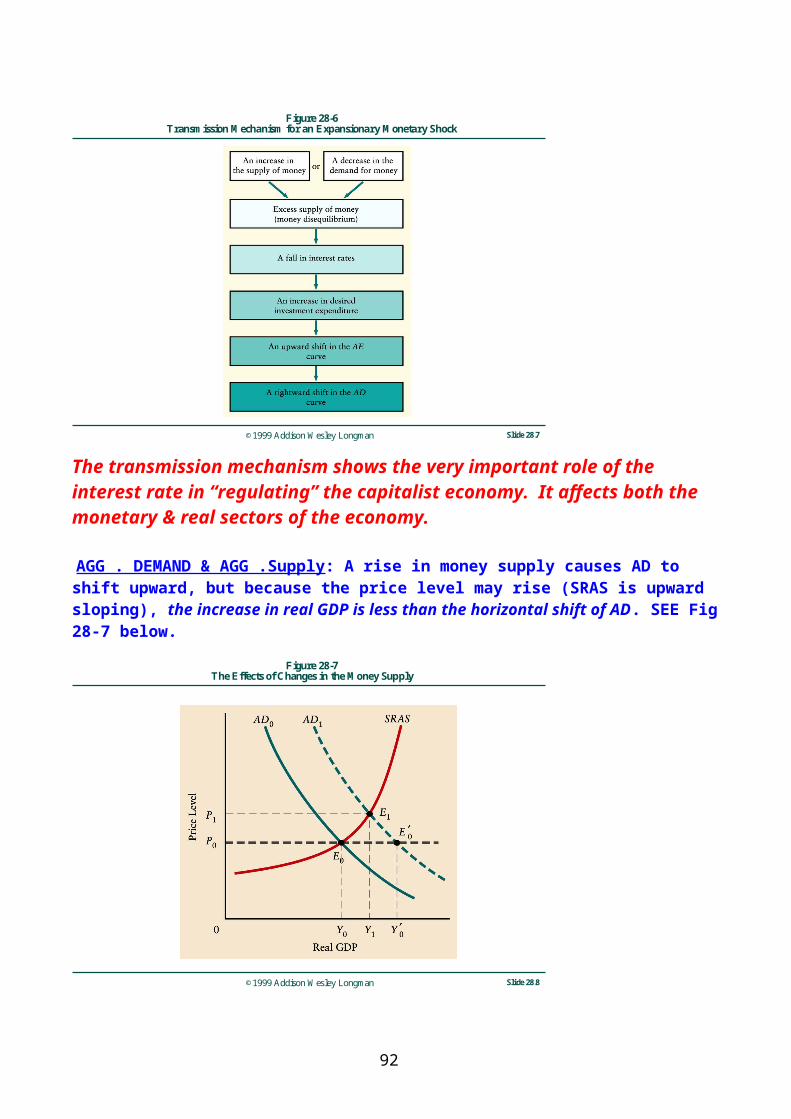
at its potential level, the only unemployment (by definition) is the NAIRU, which comprises frictional and structural unemployment.
Why Does The NAIRU Change?
1-a) An increase in the rate of growth , for example , usually speeds up the rate at which the structure of demand for labor is changing. 1-b) the adaptation of labor to the changing structure of demand, may be slowed by such diverse factors as a decline in education and new regulations that make it harder for workers in a given occupation to take new jobs in other areas or occupations.
2) Demographic Changes: Young or inexperienced workers have higher unemployment rates than experienced ones. Also, the change in social values, such as the increase in the no. of women going out for work.Learning on-the-job experience is a critical part of developing marketable labor skills, and people who suffered prolonged unemployment during their teens and twenties have been denied that experience early in their working careers. Such people may have no choice but to accept temporary jobs at low wages.3) HysteresisRecent models of unemployment show that the size of the NAIRU can be influenced by the actual current rate of unemployment. Such models get their name from the Greek word hysteresis, meaning “lagged effect”. One mechanism that can lead to hysteresis in labor markets arises from the importance of experience and on-the-job training. Suppose that a recession causes a significant group of new entrants to the labor force to encounter unusual difficulty obtaining their first jobs. When demand increases again, this group of workers will be at a disadvantage relative to workers with normal histories of experience, and the unlucky group may have unemployment rates that will be higher than average.
Another force that can cause such effect is heavily unionized labor force. This has been noticed in Western Europe. In times of high unemployment, people who are currently employed (insiders) may use their bargaining power to insure that new workers (outsiders) do not join in. If outsiders are denied access to the labor market, their unemployment will fail to exert downward pressure on wages, and the NAIRU will tend to rise.
4) Policy and Labor-Market FlexibilityOne important cause of unemployment in very general terms is inflexibility in the labor market. If workers are unable or unwilling to move between regions or between industries, then changes in the structure of the economy can cause unemployment. If it is costly for firms to hire workers then firms will find other ways of increasing output (such as switching to more capital -intensive methods of production).Any government policy that reduces labor-market flexibility is likely to increase the NAIRU.
We discuss two examples.
The first example is unemployment insurance. UI provides income support to eligible unemployed workers and thus reduces the costs to the workers of being unemployed. This income support will typically lead the worker to search longer for a new job and thus increase, the unemployment rate. As was suggested extension 31-2, this longer search may be desirable
92
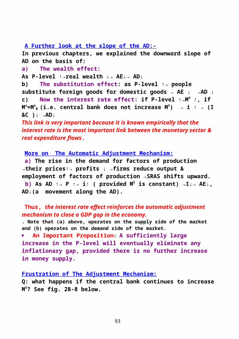
since by reducing the cost of unemployment the worker is able to conduct a thorough search for a job that is an appropriate match for his specific skills. On the other hand, if the UI system is so generous the workers have little incentive to accept reasonable jobs.The second example concerns policies designed to increase job security for workers. In most Western European countries, firms that lay off workers are required either to give several months notice before doing so, or required to make severance payments equal to several months worth of pay. But this inflexibility on the part of the firms is passed on to workers. Firms are very hesitant about hiring workers in the first place. Given this reduction in labor –market flexibility, such policies are likely to increase the NAIRU.Job security is very rare in the United States. Its rarity contributes to the general belief among economists that U.S. labor markets are much more flexible than those in Europe. Many economists see this as the most important explanation for why the unemployment rate in the United States is significantly below the unemployment rates in Europe, and has been for the past two decades.What is the situation in Saudi Arabia?
REDUCING UNEMPLOYMENT
Cyclical UnemploymentCyclical unemployment control is the subject of stabilization policy, which we have studied in several earlier chapters. A major recession that occurs because of natural causes can be encountered by monetary and fiscal policies to reduce cyclical unemployment. There is room for debate however, about how much the government can and should do in this respect. Whatever may be argued in principle, policy-makers have not yet agreed to abandon such stabilization measures in practice.
Frictional UnemploymentFrictional unemployment is a natural part of the learning process for young workers. Increasing the knowledge of workers about market opportunities may help. Unemployment insurance is one method of helping people cope with unemployment. It has reduced significantly the human costs of the bouts with unemployment that are inevitable in a changing society. Nothing however is without cost. It also contributes to unemployment, as we have already observed. Supporters of UI emphasize its benefits. Critics emphasize its costs. Workers must be actively seeking employment in order to be eligible for UI. Finally, a system of experience ratings has helped to distribute the costs more in proportion to the benefits. Under experience rating, firms with histories of sizable layoffs, pay more than those with better layoff records.
Structural Unemploymenta) There are two basic approaches to reducing structural unemployment: try to prevent the changes that the economy experiences or accept the change and try to speed up the adjustments. Workers have often resisted the introduction of new techniques to replace the older techniques at which they were skilled. Older workers may not even get a chance to start over with the new technique.
b) However, new techniques are a major source of economic growth.
c) Over the long term, policies that subsidize employment in declining industries run into increasing difficulties. Agreements to hire unneeded workers raise costs and can hasten the decline of an industry that is declining because of economic change becomes an
93

increasingly large burden on the public budget as economic forces become less and less favorable to its success. Sooner or later, public support is withdrawn, followed by a precipitous decline. There is often a genuine conflict of interest between the private interests of workers threatened by structural change & the social interest served by generating change for the benefit whole society.
CONCLUSIONHarsh critics see unemployment as proof that the market system is badly flawed. Reformers regard it as a necessary evil of the market system and a suitable object for government policy to reduce its incidence and its harmful effects. Others see it as overblown in importance and believe that it does not reflect any real inability of workers to obtain jobs if they really want to work. Whatever the case may be, unemployment is always a problem of economic, social, political, and psychological dimensions, that must be dealt with.
END OF CHAPTER 31
94

CHAPTER 32: GOVERNMENT DEBT & DEFICITS
I) DEFICIT & DEBTS: FACTS & DEFINITIONS
The Govt. Budget Constraint is:
Govt. Expenditures = Tax Rev. + BorrowingIn other words, part of govt. expenditures is financed by taxes, & part is financed by borrowing.
Govt. Expenditures = Three broad components:G+TR+(i x D) = Tax Rev. + Borrowing, Where G is govt. purchases, TR: transfer payments( such as social security, unemployment insurance, or industrial subsidies), i: interest on Govt. debt, D: total outstanding public( govt.) debt , (i x D) is the debt-service payments,
Budget Deficit= Borrowing = D (change in Public Debt) = G+TR+ (i x D)-T
Every budget deficit (BD) is financed by borrowing, which in turn adds to ( and is equal to the change in) public debt. Two points about BD:a) a change in the size of the deficit requires a change in the level of expend. relative to the level of tax revenue.b) Govt. debt will rise whenever the BD is positive. Debt will fall only if the deficit becomes negative. i.e only if there is a budget surplus.
The Primary Budget Deficit: The debt- service component of total expend. is beyond the control of govt. policy because it is determined by past govt. borrowing. In contrast, the other components of the govt. budget are said discretionary because the govt. can choose the levels of G,TR , or T. The discretionary part of the BD is called the Primary Budget Deficit = Total Deficit – Debt Service Payment
={G+TR+(i x D)-T} – (i x D)=(G+TR) – T
Where ( G+TR) is discretionary expenditures. It is called Govt's. Program Spending. It is possible that the govt. has an overall BD but a primary budget surplus ( BS). SEE FIG. 32-1 below.
95
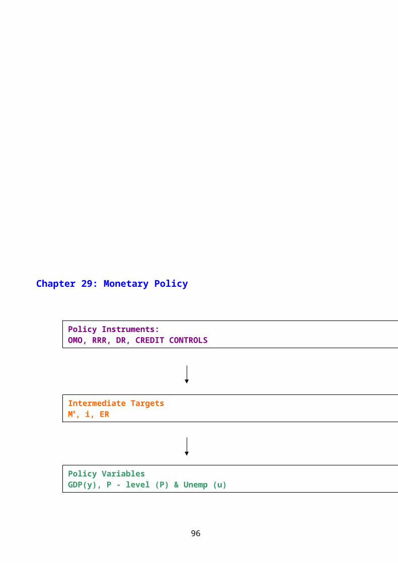
©1999 Addison Wesley Longman Slide 32.2
Figure 32-1The Government’s Budget Constraint
In both cases above, there is an overall BD. However in case i there is also a primary BD ( T< ( G+ TR). In case ii, there is a primary BS (T> (G+ TR)
Deficits & Debt in THE USA Compared to SAUDI ARABIA:SEE FIGURES 32-2-3-4:The size of govt. expenditures, revenues, BD, Primary BD, public debt, & debt- service payments may not be meaningful unless we relate them to the level of GDP. This is what the figures below are telling us about the US economy.
96
©1999 Addison Wesley Longman Slide 32.3
Figure 32-2Federal Revenues, Expenditures, and Deficits, 1962-1997 (as a percentage of GDP)
©1999 Addison Wesley Longman Slide 32.4
Figure 32-3Federal Government Net Debt (as a percentage of GDP) 1940-1997
97
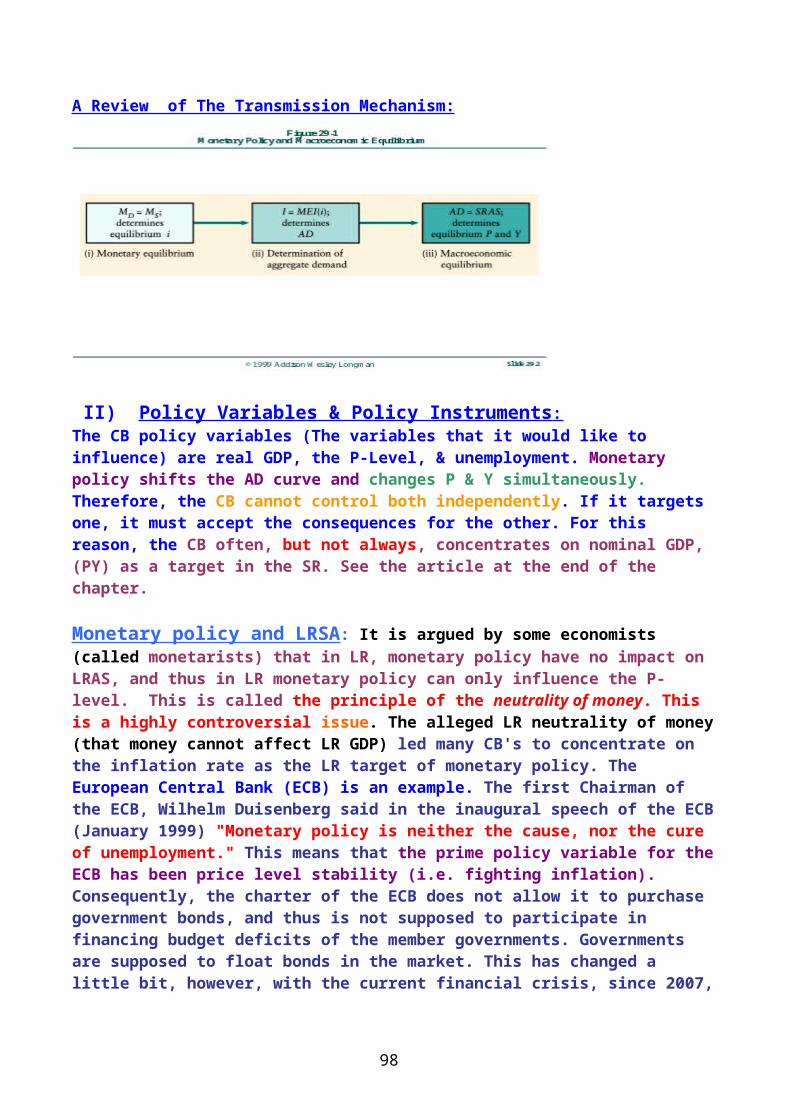
©1999 Addison Wesley Longman Slide 32.5
Figure 32-4Budget Deficit and Debt-Service Payments 1970-1997
SEE SAMA's ANNUAL REPORTS FOR DATA ON SAUDI PUBLIC DEBT & BUDGET DEFICITS
http://www.sama.gov.sa
II)DEFICITS & DEBT: SOME ANALYTICAL ISSUES
II-1)The Stance of Fiscal Policy: Expansionary or Contractionary?
a) The Budget Deficit Function: Budget Deficit= ( G + i x D ) – ( T – TR ) autonomous partially endogenous (due to policy) (a function of GDP). Thus with no changes in expend. or taxation, the BD tends to rise in recession and fall in booms. In reality, however, the govt. does use its discretion to change many variables. Thus, the BD is actually two parts:
Budget Deficit
Discretionary Cyclical(Structural)
Part of the budget deficit is due to the govt.'s own discretion (policy), but part of it is due the state of the economy (which phase of the business cycle the economy is in). To judge the stance of fiscal policy, we have to isolate one part from the other. To do this, economists speak of something called CAD.
b) CAD: The Cyclically Adjusted Deficit:
98

deficit measured assuming economy is at potential GDP (Y*). This removes the effect of the business cycle. The change in CAD determines the stance of fiscal policy: If CAD increases, it implies that fiscal policy is expansionary. Otherwise , it is contractionary . SEE FIG. 32-5 below.
©1999 Addison Wesley Longman Slide 32.6
Figure 32-5The Budget Deficit Function and Cyclical Adjustment
The govt.'s policy determines the position of the BD function. Moving from B0 to B1 in (iii ) above represents a restrictive fiscal policy.
©1999 Addison Wesley Longman Slide 32.7
Figure 32-6The Actual and Cyclically Adjusted Deficit, 1970-1997
II-2)THE DEBT-To-GDP RATIO:
99
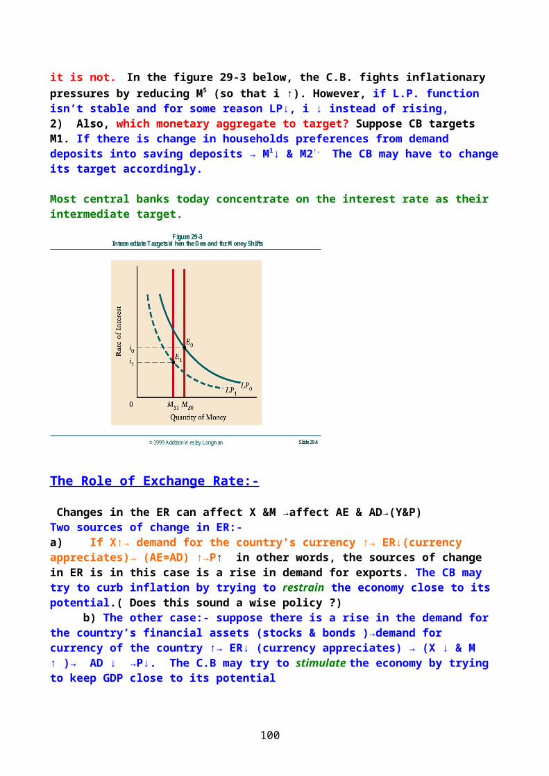
From Extension 32-1 we have:
d= X+(r-g) x d
where d: is the debt-to-GDP ratioX= is the govt. primary deficit as a percentage of GDPr= is the real interest rateg= is the growth rate of real GDP.
There are two distinct forces that tend to increase the debt-to- GDP ratio:1) If r > g, then the debt- to – GDP ratio rises( that is d will be positive).2) If the govt. has a primary BD (if X is positive), then the debt- to – GDP ratio rises.1-a) The Importance of Real interest rates: It is the real interest rate not nominal interest rate that is important to determine d. Many commentators argue that high nominal interest rates are largely responsible for increasing the govt.'s debt-service requirements & thus pushing up the deficit & the debt .This is only partially correct. The real financial liability of the govt. is determined by real stock of debt. High nominal interest rates are usually associated with high inflation which reduces the real value of govt. debt.
2-a) The Role of The Primary Deficit: If the focus is to be on the debt-to- GDP ratio, rather than the absolute size of the debt, then tracking the behavior of the overall BD is misleading. The reason is that it is possible to reduce the debt- to- GDP ratio even though the overall BD may never be eliminated, & thus even though the absolute size of the debt continues to increase.
Stabilizing The Debt-to-GDP ratio ( V. Imp): To do this the govt. must maintain certain relationship between the primary deficit, the debt-to- GDP ratio, & the values of r and g. For example, if r > g, then a govt. with a positive stock of outstanding debt must run a primary surplus in order to stabilize the debt- to- GDP ratio.
II-3) GOVERNMENT DEFICITS & NATIONAL SAVINGWe have seen in Chapter 24 that
National saving= private saving + govt. saving
An increase in govt. BD is a reduction in govt. saving and national saving. Alternatively, we can write:
National saving= private saving - govt. BD
The effect of the BD on the level of national saving thus depends on the link between BD & private saving. For example, if BD rises by SR 10 billion. If this reduction in govt. saving leads to an increase in private saving by exactly SR10 billion , there will be no change in national saving. If not, national saving will fall as a result of the BD. But what is the link between GD & private saving? Remember that govt. expend. must be paid for either by current taxes or future taxes (current borrowing ) . This implies that Gov’t Debt represents deferred liabilities for taxpayers.
100
The Ricardian Equivalence: The link between GD & private saving is associated with idea of the Recardian Equivalence, named after the Classical economist David Ricardo ( 1772-1823). The central proposition is that consumers recognize that current govt. borrowing as a future tax liability & thus view govt. borrowing as equivalent to taxes in terms of its impact on their own wealth. In other words, taxes reduce households wealth , but current govt. borrowing reduces future wealth too. Therefore , a reduction in taxes and a rise in borrowing ( or the reverse case) does not make people feel wealthier by holding govt. bonds and thus don’t increase their consumption. Thus “Ricardian” consumers faced with a change in taxes will change their private saving exactly to offset the change in govt. saving. If this is the case fiscal policy may not be effective to manage the economy.
Why this might not be so?1) short-sightedness: many people don’t care much about the future and spend accordingly.2) uncertainty about future govt. fiscal policy: would reductions in taxes today be matched with more taxes tomorrow or reduced govt. expenditures?
The issue of the Recardian Equivalence is an empirical one. Most evidence suggests that it does not hold completely and hence suggests a negative relationship between GD & national saving. In this case expantionary fiscal policy would stimulate private consuption and GDP.
III)THE EFFECTS OF GOVERNMENT DEBT & DEFICITSDoes the govt. BD crowd out private economic activity? Does it harm future generations? Does hamper the conduct of economic policy?
III-1) DO DEFICITS CROWD OUT PRIVATE ACTIVITY?
d) Investment in Closed Economies: in a closed economy the amount of national saving exactly equals the amount of domestic investment. Suppose govt. reduces taxes and increases borrowing. What is the effect on domestic investment? This depends on the degree that taxpayers are Ricardian—that is on the degree to which taxpayers recognize that today's deficit must be financed by higher future taxes. If taxpayers are not fully Ricardian , then private saving will rise by less than the fall in govt. saving. This implies a decrease in the supply of national saving. The resulting excess demand for funds will put upward pressures on domestic real interest rates. The components of AD that are sensitive to interest rates- investment in particular- will fall. This is called the crowding out of domestic investment. SEE FIG. 32-7.
101
©1999 Addison Wesley Longman Slide 32.8
Figure 32-7The Crowding Out of Investment
b) Net Exports in Open Economies:
If the government reduces taxes, it thus increases its budget deficit. Furthermore, suppose that taxpayers are not purely Ricardian, so that private saving rises by less than the fall in government saving. What is the effect of such a fall in national saving in an open economy? As domestic real interest rates rise in the country, foreigners are attracted to the higher-yield domestic assets and thus foreign financial capital flows into the country, thereby dampening the initia1 increase in domestic interest rates. However, since U.S. dollars are required in order to buy U.S. interest-earning assets, this capital inflow increases the demand for U.S. dollars and thus increases the external value of the dollar (the U.S. dollar appreciates).
This appreciation makes U.S. goods more expensive relative to foreign goods, inducing an increase in imports and reduction in exports, thereby reducing U.S. net exports. In an open economy, therefore, a rise the government deficit leads to an appreciation in the currency and to a crowding out of net exports.
In an open economy instead of driving up interest rates sufficiently to crowd out private investment, the government budget deficit tends to attract foreign financial capital, appreciate the currency, and crowd out net exports.
A Closed Economy: The overall effect of the increase in the government deficit in a closed economy is a rise in the real interest rate and a fall in the level of domestic investment. However, less current investment means that there will be a lower stock of physical capital in the future, and-thus 'reduced ability to produce goods and services in the future. This reduction in future production possibilities, which implies lower consumption levels for future generations, is the long-term burden of the debt.
An Open Economy: The overall effect of the increase in the government deficit in an open economy is an appreciation of the currency and a reduction in net exports. Recall from
102
Chapter 24, however, that such a reduction in net exports implies a reduction in the country's national asset formation. This in turn increases the need for the domestic economy to make interest payments to foreigners in the future. Thus, in an open economy, an increase in the government budget deficit does not lead to a reduction in the domestic capital stock but less of it is owned by domestic residents. This reduced ownerships lowers the domestic residents' future stream of income because payments must be paid to the foreign owners of the domestic capital stock. This reduction in the future stream of income for domestic residents is the long term burden of the public debt in an open economy.
In both cases, there is less output available for consumption by future generations of domestic residents. This reveals an important aspect of the costs associated with government debt and deficits.
This last sentence suggests that current government deficits are always financing goods and services that are provided to the current generation. But is this really true? Some government spending is on good and services that will continue to be used well into the future. For example if the government increases- its current borrowing to finance the building of bridges or the expansion of highways, future generations will receive some of the benefits of this government spending.
Whether current government deficits impose a burden on future generations, depends upon the nature of the government goods and services being financed by the deficit. At one extreme, the govern borrowing may finance a project that generates a return only to future generations, and thus the future generations may not be made worse off by today's budget deficit. An example might be the government's financing medical research projects that generate a return only-in the distant future.
The concern that deficits may be inappropriately placing a financial burden on future generations has led some economists to advocate the idea of budgeting by the government. Under this scheme, the government would essentially- classify all of its expenditures either consumption or investment; the former would be spending that mostly benefits the current generation while the latter would be spending that mostly benefits future generations.
DOES GOVERNMENT DEBT HAMPER ECONOMIC POLICY?
The costs imposed on future generations by government debt are very real. Unfortunately, the fact that these cost sometimes occur in the very distant future often leads us to ignore their importance. But other costs associated with the presence of government debt are more immediately apparent. In particular government debt may make the conduct of monetary and fiscal policy more difficult.
Monetary Policy
Recall that the long-term goal of monetary policy is influence ~rate-o[inflation,- and that the Federal Reserve's primary instrument is its control over the rate of growth of money supply. In Chapter 30 we saw that sustained inflation possible only when the Fed permitted a sustained growth in the money supply. These facts appear to suggest that government deficits cause inflation.
103

Note, however, that when the government operates a budget deficit and is thus borrowing funds, it can borrow from households or firms in the private sector, it can borrow from the Federal Reserve. But not all of these are these are same in. term of effect on the money supply.
As we saw in Chapter 29, changes in the Fed's balance sheet are central to changes in the money supply. And, when the government borrows from either the private sector or from foreigners~ there is no change in the Fed's balance sheet, and thus no change in the money supply. In contrast, if the government borrows from the Fed (an open-market purchase by the Fed), this increases the Fed's assets (government securities) and similarly increases the Fed's liabilities (currency). Thus it is no necessary link between budget increase the money supply.
To summarize the foregoing argument, unless the central bank finances some of the budget deficit, there is no necessary link between budget deficits (fiscal policy) and inflation (monetary policy). Thus a budget deficit can cause a one time increase in the price level, but, unless the Fed increases the rate of growth of the money supply, it will not cause a sustained inflation.
The last point suggests that the independence of the central bank from the government deficits and inflation. For example, if the government were able to force the central bank to finance some fraction of government deficits-referred to as monetizing the deficit-then government deficits would clearly-1ead to the creation of money and eventual inflation. Though budget deficits need not be inflationary, their accumulated value over many years-the stock of government debt: can still make monetary policy more difficult. To see how a large stock of government debt can hamper the conduct of monetary policy, consider a country that has a high debt to GDP ratio and that has a real interest rate above the growth rate of GDB. As we saw earlier in this chapter, the debt-to- GDP ratio will continue to grow in this situation unless the government starts running significant primary budget surpluses. Such fears of future debt monetization will lead to expectations of future inflations of thus will put upward pressure on nominal interest rates and on some prices wages.
How does the presence of government debt affect the government's ability to conduct such counter cyclical fiscal policy?
∆d = x + (r -g) X d
Thus there may well be room for the government to increase the primary deficit-either by increasing the programs spending or by reducing tax rates without generating a large increase in the debt-to-GDP ratio.
In this case the high value of d means that even in the absence of a primary budget deficit, d will be increasing quickly. Thus any increase in the primary deficit brought about by the counter-cycled fiscal policy runs the danger of generating increases in the debt-to-GDP ratio that may be viewed by creditors as unsustainable.A tradeoff therefore appears to exist between the desirable short-run stabilizing role of deficits and the undesirable long-run costs of government debt. This tradeoff has been the source of constant debate. Here we examine some possible solutions.
104
Before examining some proposals for dealing with deficits, however, note that not everyone agrees that government deficits and debt represent a problem. Some economist that take the view that Ricardian equivalence does hold and thus budget deficits do not lead to a crowding out of investment or net exports and thus there is no long-term burden associated with the public debt. Other economists accept the view that sufficiently high deficits and debt can indeed represent a problem, but argue that the current debt-to-GDP ratio in the United States, about 48 percent, is not high enough to cause concern.
Though these debates might be reasonable, there are some unreasonable arguments for why government debt is a problem. For example, many people argue that the main problem with the government debt is that much of it is held by foreigners and that such foreign ownership is bad, because interest payments are remitted abroad, reducing the income available for Americans. Such claims have even inspired a proposal that the U.S. government issue new "U.S.-only" bonds to Americans and then use the newly raised funds to redeem foreign-held government debt.
ANNUALY BALANCED BUDGETS
Even with the success that the Clinton Administration has had in reducing the budget deficit-from $290 billion in 1992 to $22 billion in 1997, and a likely balanced budget by 1999-there is still considerable support among leading members of Congress for an amendment to the u.s. Constitution that would require the federal government to balance, its budget on an annual basis.
Balancing the budget on an annual basis would extremely difficult to achieve. The reason is that a significant portion of the government budget is beyond the short-term control of the government, and a further large amount is hard to change quickly. For example the entire debt-service component of government expenditures is determined by past borrowing and thus cannot be altered by the current government. In addition, as we saw in our discussion of the cyclically adjusted deficit, changes in national income (real GDP) that are-beyond the control government lead to significant changes in tax revenues (transfer payments) and thus generate significant changes in the budget deficit. Even if it were possible for the government to perfectly control its path of spending and revenues on a year-to-year basis, it would probably be undesirable to balance the budget every year. We saw above government-tax-revenues (net of transfers) tend to fall in recessions and raise in-booms. In contrast, the level of government purchases is more or less dependent of the level of national income. With a balanced budget, government expenditures would be forced to adjust to the changing level of tax revenues. In a recession, when tax revenues -naturally decline, a balanced budget would require either a reduction in government expenditures or an increase in tax rates, thus generating a major destabilizing force on national income. Similarly, as tax revenues naturally rise in an economic boom, the balanced budget would require either an increase in government expenditures or a reduction in taxes, thus risking an over-heating of the economy.
An annually balanced budget would accentuate the swings in real GDP.
CYCLICALLY BALANCED BUDGETS One alternative to the extreme policy of requiring an annually balanced budget is to require that the government budget be balanced over the course of a full economic deficits would6epermitted in recessions as long as they were matched by surpluses in booms. In
105
principle, this is a desirable treatment of the trade off between the short-run benefits of deficits and the long-run costs, of debt.
Although more attractive in principle than the annually balanced budget, a cyclically balanced budget would carry problems of its own. Congress might well spend in excess of revenue in one year,. leaving the next Congress with the obligation of spending less than current revenue ,in following years. Could
©1999 Addison Wesley Longman Slide 32.9
Figure 32-8Balanced and Unbalanced Budgets
such an obligation to balance the budget over a period of several years bema-de-binding? It could be made a legal requirement through-ah-act of Congress. Indeed, both the Budget Enforcement Act of 1990 and the Qmnibus Budget Reconciliation Act of 1993 has taken this direction (see Application 32-2). These laws do not require balance over the cycle, but they do limit overall spending while still allowing automatic stabilizers to operate. However, what Congress does, Congress can also undo.
Perhaps the most important problem with a cyclically balanced budget is an operational one. In order have a law that requires the budget to be balanced over the cycle. it is necessary to be able to define the unambiguously. But there will always be disagreement about what stage of the cycle the economy is currently in, and thus there will be disagreement about the current government should be increasing or reduction its deficit. Compounding this problem is the fact that politicians will have a stake in the identification of the cycle.ALLOWING FOR GROWTHA further problem with any policy that requires a balanced budget whether over one year or over the business cycle is that the emphasis is naturally on the overall budget deficit. But, as we saw earlier in this chapter, what determines the change in the debt-to-GDP ratio is the growth of the debt relative to the growth of the economy. With a growing economy, it is possible to have positive overall budget deficits and thus a growing debt and still have a falling debt to GDP ratio. Thus, to the extent that the debt-to-GDP ratio is the relevant gauge of a country’s debt problem, focus should be placed on the debt-to-GDP ratio rather than directly on the budget deficit.
106

Some economies view a stable (or falling) debt-to-GDP ratio as the appropriate indicator of fiscal prudence. Their view permits a deficit such that the stock of debt grows no faster than GDP.
END OF CHAPTER 32
Exchange Rates and the Balance of Payments CH.37
The Exchange Rate: The price of one currency in terms of another. Usually, it is the price of a unit of foreign currency in terms of a local currency. Example: ($1=SR.3.75).Foreign Exchange: Holdings of a country o f foreign currencies and financial assets denominated in foreign currencies. Currency Appreciation: Arise in the external value of home currency >>>According to the above definition of the ER, the Exchange rate will decrease. The opposite will happen if the currency depreciates.Note: When one currency appreciates, the other depreciates. See Fig.37.1
107
©1999 Addison Wesley Longman Slide 37.2
Figure 37-1The Dollar-Yen Exchange Rate, 1972-1998
The Balance of Payments (BOP): It is an accounting record of all transactions between a country and the rest of the world.*Sales of any assets ( real or financial) or services >>> Receipts >>> Credit to BOP. *Purchases of any assets (real or financial) or services >>> payments >>> debit to BOP.
Table 37-1.U.S Balance of Payments,1997, (Billions of dollars)I- CURRENT ACCOUNT(a) Trade AccountMerchandise exports +679.3Service exports +258.3Merchandise imports -877.3Service imports -170.5 Trade balance -110.2(b) Capital-Service AccountNet investment income (including Unilateral transfers) -45.0 Current Account balance -155.2II- CAPITAL ACCOUNT Net change in U.S. investments abroad [capital outflow (-)] -477.5 Net change in foreign investments In the U.S [capital inflow (+) 717.6 =====Capital Account balance +240.1III- OFFICIAL FINANCING ACCOUNTChange in official reserves [increases (-) -1.0Change in liabilities to official foreign agencies[(increases (+)] +15.8 Statistical Discrepancy -99.7 =====Official Financing balance -84.9 BALANCE OF PAYMENTS 0.0The overall balance of payments always balance, but individual components do not have to
108
Structure of BOP: (Table 37.1 above):1- Current Account: a) Trade Account. b) Capital Service Account (net income from foreign investment from both goods and services).2- Capital Account: _ Foreign investment in the country >>> Capital inflow >>> Receipts >>> credit to BOP Our investment abroad >>> Capital outflow >>> Payments >>> Debits to BOP.a) Short Term Capital Movements: Buying & selling short term financial assets such as bank accounts or treasury bills b) Long Term Capital Movements: Purchasing or selling long term financial assets and/or physical assets…*if the long term capital is for a voting, or controlling share, it is called Foreign Direct Investment (FDI) *if the long term capital is NOT for voting share >>>It is a Portfolio Investment. 3- Official Reserve (Settlement) Account: transactions of the central bank buying and selling foreign currencies, foreign financial assets, gold and SDR.*Note: BOP must balance >>> sum of the sub-accounts must be zero. However, this does not mean that each account must be zero.*Balance >>> Total Receipts = Total Payments >>> (Cr+Kr+Fr) = (Cp+Kp+Fp) >>> (Cr-Cp) + (Kr-Kp) + (Fr-Fp) = 0*Surplus in one or two accounts >>> Deficit in at least one account…WHY? In other words, a deficit in one or two accounts, must be financed by a surplus in the other account(s)*Ex., a favorable balance in the current account (a Surplus) must be either invested abroad (Capital Outflow) >>> Capital account is negative >>> and/or the official reserves balance must decrease. What does it mean that the official reserves balance decrease?It means that the central bank would be buying foreign exchange from the private sector.* If the other two accounts of the BOP are in surplus, the central bank is adding to its reserves.*In day-to-day language of news, a BOP is: Current Account + Capital Account*Under flexible exchange regime, the official reserve account = 0, because central bank does not need to intervene in the foreign exchange market:
BOP = (Cr-Cp) + (Kr-Kp) = 0 (Cr-Cp) = - (Kr-Kp)
* This implies that a deficit in one account must be balanced by a surplus in the other account.*National Assets Formation = I + (X-M). Since the surplus of the current account is invested abroad >>> an increase the size of national assets. Both domestic
109
investment and surplus in current account contribute to national assets & thus generate incomes to the country. This is a very important concept of macroeconomics.Students may visit www.sama.gov.sa for information on Saudi balance of payments, and other info. on the Saudi economy in general.
* The Sources of Foreign Exchange Market: 1- Exports: These are payments by foreigners.2- Capital Inflow: When foreigners buy some of the country’s financial assets and/or physical assets. Example: Foreign companies invest in Saudi petrochemicals or telecommunication sector, 3- Reserve Currency: Changing the country's portfolio of foreign exchange.
* Supply and Demand Curves of Foreign Exchange: Fig.37.2
©1999 Addison Wesley Longman Slide 37.3
Figure 37-2The Market for Foreign Exchange
- On the Supply Curve: Suppose the Yen appreciates >>> $/Yen will increase >>> Japanese find it cheaper to buy $ and American products >>> Japanese supply more Yen (the quantity supplied of Yen will increase).- On the Demand Curve: American finds Yen more expensive >>> they demand less Yen and Japanese products >>> the quantity demanded of Yen will decrease.* Determination of Exchange Rate: Generally, there are three major ER regimes:1) A Country could choose a fixed exchange rate against another currency (or gold).2) Completely flexible (floating) exchange rate >>> exchange rate determined by the market.3)Between these two extremes, there could be may intermediate arrangements such as adjustable peg( where the ER is essentially fixed, but adjusted once- and- a while), a managed float( where the ER is essentially floating but the central bank seeks to have
110
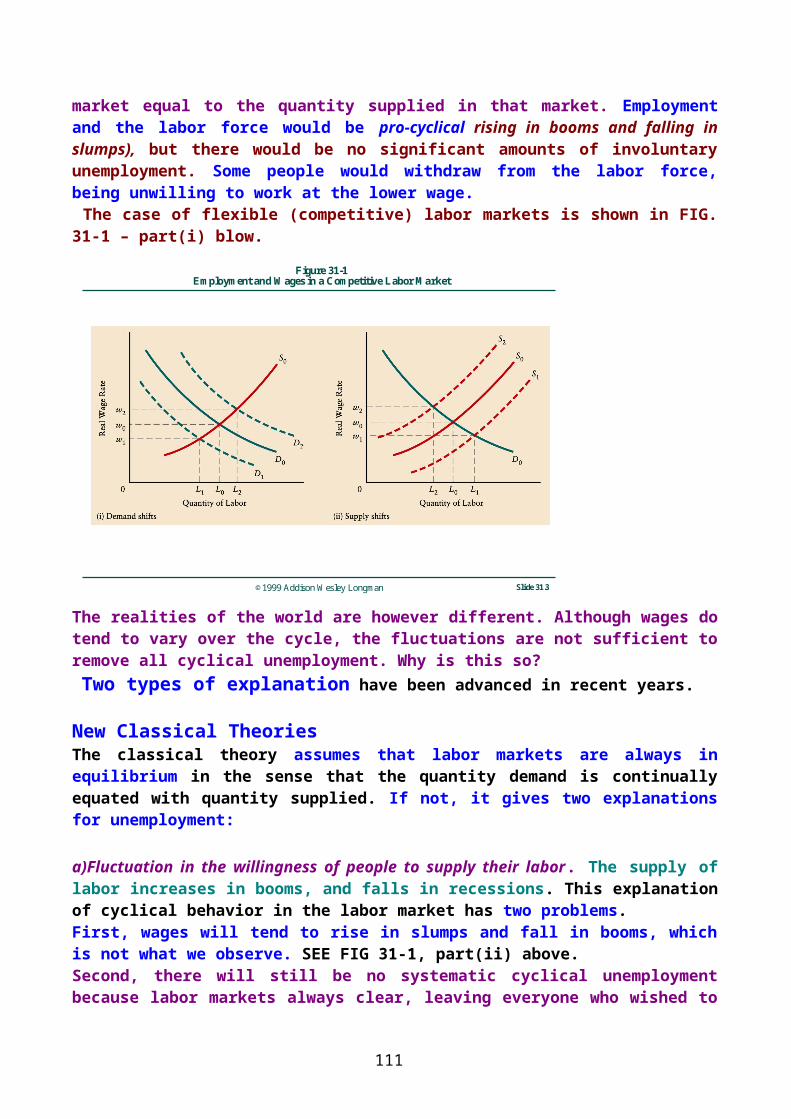
some stabilizing influence. However it does not try to fix it at some publicly announced value), and pegging against a basket of currencies. See Fig.37-3 below.
©1999 Addison Wesley Longman Slide 37.4
Figure 37-3Fixed and Flexible Exchange Rates
_ At e1: the value of the home currency is kept artificially low >>> X will increase and M will decrease >>> C\A tend to a surplus. Also, the low value of home currency may encourage an inflow of foreign investment >>> the K/A tend to a surplus. >>> As a result of both sub-accounts, foreign reserves increase >>> central bank purchases the surplus of FR to maintain exchange rat at e1 >>> (Fp> Fr)._ At e2: Home currency is kept artificially high >>> an opposite scenario takes place. *Causes of Changes in Exchange Rates:
111
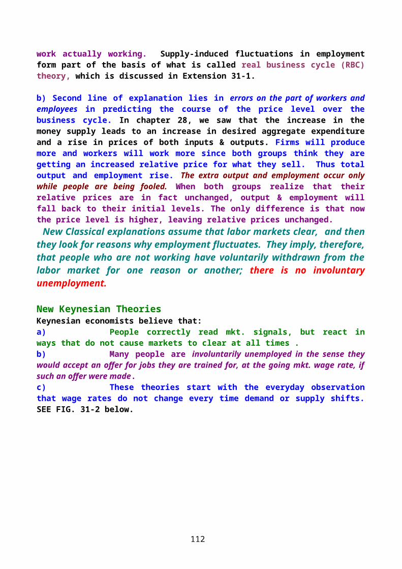
©1999 Addison Wesley Longman Slide 37.6
Figure 37-4Changes in Exchange Rates
1-A Rise in the Prices of Exports: Assume elasticity of exports ( X >1) >>> receipts (supply) of foreign currency will decrease ( TRX= PX.QX ) >>> at the same time, demand for home currency will decrease >>> supply curve for foreign currency will shift upward (Panel ii)>>> ER will increase >>> home currency will depreciate.)2-A Rise in the Prices of Imports: Assume elasticity ( M >1) >>> Payments for F.C decrease ( TPM= PM.QM ) >>> demand curve for foreign currency will shift downward (Panel i, Note: the shift of the D- curve in the fig. is wrong. It should be downward))>>> at the same time demand for home currency increases, and ER will decrease >>> home currency will appreciate.Note: the assumption about elasticity is very crucial about what should happen to the ER.3-Changes in the Overall Price Levels: a) Equal inflation in both countries: if home & foreign prices change in the same direction and at the same magnitude >>> terms of trade (PX/PM) is not affected >>> NO effect on the exchange rate.b) Inflation in Only One Country: >>> terms of trade are disturbed >>> exchange rate will change. C) Inflation at Unequal Rates: Here also the terms of trade are disturbed >>> exchange rate will change.However in all cases, remember the assumption about the elasticity (EX > 1 & EM > 1). The direction of change depends on that assumption.4-Capital movements: a) Short term capital movement: Most important factor is changes in interest rates. If the interest rate of a country increases >>> its financial assets are more attractive >>> demand for the country’s currency will increase >>>its exchange rate will decrease >>> its currency will appreciate.
112
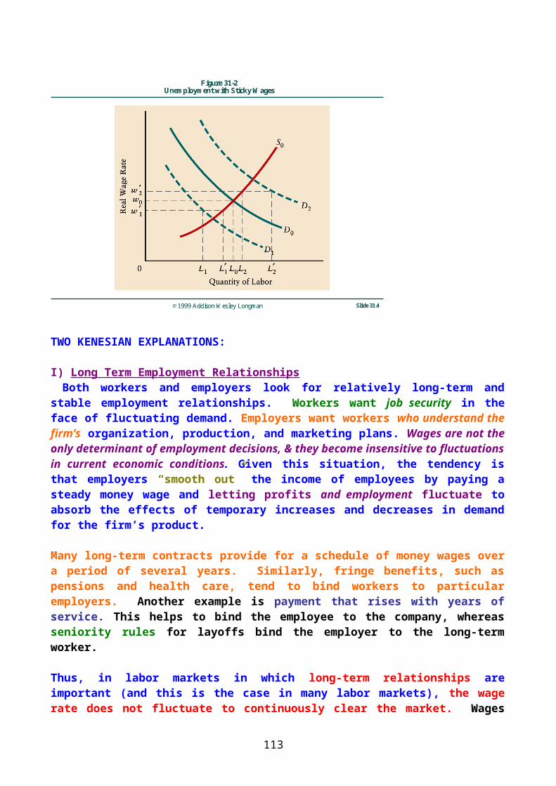
b) Speculation about future value of a country's exchange rate: If a country's ER is expected to appreciate in the future, investors rush to buy assets denominated in that currency. The country's currency appreciates, & visa versa.c) Long term capital movements: are largely affected by long term expectations of about profit opportunities in a country and the long term value of its exchange rate.5-Structural changes: Long term changes in the economy may affect long term terms of trade & thus long term ER. Such changes may be affected by: a) Changes in cost structure of production, such as a permanent rise in real wages and real interest rates, b) R&D that leads to growth in some sectors at expense of others, c) discovery of natural resources… The development of natural gas in the Netherlands in 1960s, and the development of North Sea oil in the UK in 1970s brought about the so-called the Dutch Disease in both countries. It led to the appreciation of Dutch Guilder & the sterling Pound respectively and had a negative effect on Dutch & British exports. d) Major changes in the terms of trade may generate structural changes and affect exchange rates, as happened in 1997-1998 when commodity prices in many countries declined and affected the currencies of major commodity exporters such as Australia, New Zealand, Canada and South Africa. Also, in that period, oil prices severely declined and had a profound effect on the oil exporting countries. * Behavior of Exchange Rate: - The Law of one price: In the absence of all trade barriers, the price of identical baskets of goods should be the same in all countries. If not, arbitrage will take place until prices are equalized.-The Purchasing Power Parity Exchange Rate (the PPP exchange rate): It is the exchange rate that guarantees the validity of the law of one price. This means If the market ER is equal to the PPP rate, the purchasing power of a currency should the same both at home & abroad. Or, the price of identical goods should be the same in the two countries when expressed in the same currency. This means: Ph= e X Pf
-Example: Suppose that the price of a Shawrma Sandwich in Dhahran is SR10 and the price of the same Sandwich in Bahrain is 1 Dinar. If the exchange rate is: BD 1 = SR 10 >>> the exchange rate makes the cost of the Sandwich the same across the two countries. This exchange rate is called the PPP rate. If the exchange rate is different from PPP rate >>> currency is either overvalued or undervalued.-Definition (V.V. Imp.): An overvalued currency is one that has a stronger purchasing power abroad than it has at home. In this case, imports are encouraged and exports are discouraged. The BOT and the BOP will tend to be in deficit. An undervalued currency (abroad) implies the opposite.-Note that: the PPP rate is an equilibrium exchange rate. So, PPP theory of exchange rate is an equilibrium theory of the ER. It says that in the long run, exchange rates should adjust to make the prices of identical goods the same across countries when expressed in the same currency.
113
Why the absolute version of PPP theory may NOT hold???1) Differentiated products that may entre into the calculation of different price indexes. This makes basket of goods are not identical across countries. Consequently, it renders the comparison of price indexes difficult.2) Costly information about prices.3) The theory assumes the absence of trade barriers. In reality, there are many trade barriers. Thus, the law of one price can be validated.4) Price indexes include prices of both tradable and non-tradable goods. Only tradable goods affect exchange rate.5) Changes in relative prices of some goods affect supply and demand of foreign exchange rate & thus affect exchange rates. This may happen while the overall price levels are NOT affected.*The Relative (Weaker) Version of PPP Theory of Exchange Rate: Because of the reasons explained above, economists came up with concept of relative PPP theory; E^ = Π^
h -Π^f
This says that the percentage change in the ER is equal to the difference in inflation rates between the two countries. -PPP in the short run (Effect of speculation): Some economists argued that speculation in currencies may not be bad, for it will eventually bring exchange rates to their PPP values. However, this may be true only if speculators know that deviations from PPP are small and short-lived.-Experience shows that under flexible exchange rates, swings around PPP have been wide and long lasting. Changes in interest rates have been a major cause of swings in exchange rates. Whatever the causes of swings, speculation has been destabilizing to exchange rate. *Exchange Rates, Interest Rates and Monetary Policy:*If monetary policy is tight >>> interest rate will increase >>> exchange rate will decrease >>> the currency will appreciate >>> Expenditures on (I,C,X) will decrease and M will increase >>> AD (AE) will decrease >>> a recessionary gap may take place. *The appreciation of the currency will continue until it has appreciated enough so that investors expect a future depreciation that just offsets the interest premium for investing in the securities of that country.*The implication of this theory is that a central bank that is seeking to use its monetary policy to achieve its domestic policy targets may have to put up with large fluctuations in the ER.* Other countries may be affected by the monetary a policy of another country. The interest rate differential among countries >>> capital outflows from other countries into the country with a higher interest rate. Also, the appreciation of one country's currency implies depreciation of currencies of other countries. This stimulates exports from other countries to the country that started a tight monetary policy. As a result
114
wages & prices in other countries rise. This leaves these countries with the uncomfortable choice of either following the example of the other country (raising interest rates), or maintaining a lower interest rate and suffer inflation. This scenario assumes that the capital markets of the concerned countries are integrated.*In 1980s when the US tightened it monetary policy, other central banks in major industrial countries were forced to follow the US example, which led to sever world recession. See Application 37-2 on Beggar-My- Neighbor Policies, Past And Present.
END of CHAPTER 37
115