Embed Size (px)
Citation preview
Doc.Math. J.DMV 213
Invariant Inner Product in Spaces of
Holomorphic Functions
on Bounded Symmetric Domains
Jonathan Arazy and Harald Upmeier
1
Received: March, 24, 1996
Revised: August, 8, 1997
Communicated by Joachim Cuntz
Abstract. We provide new integral formulas for the invariant inner prod-
uct on spaces of holomorphic functions on bounded symmetric domains of
tube type.
1991 Mathematics Subject Classi�cation: Primary 46E20; Secondary 32H10,
32A37, 43A85
0 Introduction
Our main concern in this work is to provide concrete formulas for the invariant inner
products and hermitian forms on spaces of holomorphic functions on Cartan domains
D of tube type. As will be explained below, the group Aut(D) of all holomorphic
automorphisms of D acts transitively. Aut(D) acts projectively on function spaces
on D via f 7! U
(�)
(')f := (f � ') (J')
�=p
; ' 2 Aut(D); � 2 C, but these actions
are not irreducible in general. The inner products we consider are those obtained
from the holomorphic discrete series by analytic continuation. The associated Hilbert
spaces generalize the weighted Bergman spaces, the Hardy and the Dirichlet space. By
\concrete" formulas we mean Besov-type formulas, namely integral formulas involving
the functions and some of their derivatives. Possible applications include the study
of operators (Toeplitz, Hankel) acting on function spaces and the theory of invariant
Banach spaces of analytic functions (where the pairing between an invariant space
and its invariant dual is computed via the corresponding invariant inner product).
Our problem is closely related to �nding concrete realizations (by means of inte-
gral formulas) of the analytic continuation of the Riesz distribution. [Ri], [Go], [FK2],
Chapter VII.
1
Authors supported
by a grant from the German-Israeli Foundation (GIF), I-415-023.06/95.
Documenta Mathematica 2 (1997) 213{261
214 Arazy and Upmeier
In principle, the analytic continuation is obtained from the integral formulas
associated with the weighted Bergman spaces (i.e. the holomorphic discrete series)
by \partial integration with respect to the radial variables". This program has been
successful in the case of rank 1 (i.e. when D is the open unit ball of C
d
, see [A3]).
The case of rank r > 1 is more di�cult, and concrete formulas are known only in
special cases, see [A2], [Y4], [Y1], [Y2].
This paper consists of two main parts. In the �rst part (Sections 2, 3, and 4) we
develop in full generality the techniques of [A2], [Y4], and obtain integral formulas
for the invariant inner products associated with the so-called Wallach set and pole
set. In the second part (section 5) we introduce new techniques (integration on
boundary orbits), to obtain new integral formulas for the invariant inner products
in the important special cases of Cartan domains of type I and IV. This approach
has the potential for further generalizations and applications, including the in�nite
dimensional setup.
The paper is organized as follows. Section 1 provides background information on
Cartan domains, the associated symmetric cones and Siegel domains and the Jordan
theoretic approach to the study of bounded symmetric domains [Lo], [FK2], [U2].
We also explain some general facts concerning invariant Hilbert spaces of analytic
functions on Cartan domains and the connection to the Riesz distribution. Section 2 is
devoted to the study of invariant di�erential operators on symmetric cones. We study
the \shifting operators" introduced by Z. Yan and their derivatives with respect to
the \spectral parameter". Section 3 is devoted to our generalization of Yan's shifting
method, to �nd explicit integral formulas for the invariant inner products obtained
by analytic continuation of the holomorphic discrete series. In section 4 we study the
expansion of Yan's operators, and obtain applications to concrete integral formulas
for the invariant inner products. Some of these results were obtained independently
by Z. Yan, J. Faraut and A. Kor�anyi, [FK2], [Y4]. We include these results and our
proofs, in order to make the paper self contained, and also because in most cases our
results go beyond the results in [FK2], [Y4].
In section 5 we propose a new type of integral formulas for the invariant inner
products. These formulas involve integration on boundary orbits and the applica-
tion of the localized versions of the radial derivative associated with the boundary
components of Cartan domains. We are able to establish the desired formulas in the
important special cases of type I and IV. The techniques established in this section
can be used in the study of the remaining cases.
Finally, in the short section 6 we use the quasi-invariant measures on the bound-
ary orbits of the associated symmetric cone in order to obtain integral formulas for
some of the invariant inner products in the context of the unbounded realization of the
Cartan domains (tube domains). These results are essentially implicitly contained in
[VR], where the authors use the Lie-theoretic and Fourier-analytic approach to analy-
sis on symmetric Siegel domains. We use the Jordan-theoretic approach which yields
simpler formulation of the results and simpler proofs.
Acknowledgment: We would like to thank Z. Yan, J. Faraut, and A. Kor�anyi for
sending us drafts of their work and for many stimulating discussions. We also thank
the referee for valuable comments on the �rst version of the paper.
Documenta Mathematica 2 (1997) 213{261
Invariant Inner Products 215
1 Preliminaries
A Cartan domain D � C
d
is an irreducible bounded symmetric domain in its Harish-
Chandra realization. Thus D is the open unit ball of a Banach space Z = (C
d
; k � k)
which admits the structure of a JB
�
-triple, namely there exists a continuous mapping
Z � Z � Z 3 (x; y; z) ! fx; y; zg 2 Z (called the Jordan triple product) which is
bilinear and symmetric in x and z, conjugate-linear in y, and so that the operators
D(x; x) : Z ! Z de�ned for every x 2 Z by D(x; x)z := fx; x; zg are hermitian,
have positive spectrum, satisfy the "C
�
-axiom" kD(x; x)k = kxk
2
, and the operators
�(x) := iD(x; x) are triple derivations, i.e. the Jordan triple identity holds
�(x)fy; z; wg = f�(x)y; z; wg+ fy; �(x)z; wg+ fy; z; �(x)wg; 8y; z; w 2 Z:
The norm k � k is called the spectral norm. We put also D(x; y)z := fx; y; zg. An
element v 2 Z is called a tripotent if fv; v; vg = v. Every tripotent v 2 Z gives rise to
a direct-sum Peirce decomposition
Z = Z
1
(v) + Z
1
2
(v) + Z
0
(v); where Z
�
(v) := fz 2 Z; D(v; v)z = �zg; � = 1;
1
2
; 0:
The associated Peirce projections are de�ned for z
�
2 Z
�
(v), � = 1;
1
2
; 0, by
P
�
(v)(z
1
+ z
1
2
+ z
0
) = z
�
; � = 1;
1
2
; 0:
In this paper we are interested in the important special case where Z contains
a unitary tripotent e, for which Z = Z
1
(e). In this case Z has the structure of a
JB
�
-algebra with respect to the binary product x � y := fx; e; yg and the involution
z
�
:= fe; z; eg, and e is the unit of Z. The binary Jordan product is commutative,
but in general non-associative. The triple product is expressed in terms of the binary
product and the involution via fx; y; zg = (x�y
�
)�z+(z �y
�
)�x� (x�z)�y
�
. In this
case the open unit ball D of Z is a Cartan domain of tube-type. This terminology is
related to the unbounded realization of D, to be explained later.
Let X := fx 2 Z;x
�
= xg be the real part of Z. It is a formally-real (or
euclidean) Jordan algebra. Every x 2 X has a spectral decomposition x =
P
r
j=1
�
j
e
j
,
where fe
j
g
r
j=1
is a frame of pairwise orthogonal minimal idempotents in X , and
f�
j
g
r
j=1
are real numbers called the eigenvalues of x. The trace and determinant (or,
\norm") are de�ned in X via
tr(x) :=
r
X
j=1
�
j
; N(x) :=
r
Y
j=1
�
j
respectively, and they are polynomials on X . The maximal number r of pairwise
orthogonal minimal idempotents in X is called the rank of X . The positive-de�nite
inner product in X , hx; yi = tr(x � y); x; y 2 X , satis�es
hx � y; zi = hx; y � zi; x; y; z 2 X:
Equivalently, the multiplication operators L(x)y := x � y; x; y 2 X , are self-adjoint.
The trace and determinant polynomials, as well as the multiplication operators, have
unique extensions to the complexi�cation X
C
:= X + iX = Z. Let
:= fx
2
;x 2 X;N(x) 6= 0g:
Documenta Mathematica 2 (1997) 213{261
216 Arazy and Upmeier
Then is a symmetric, open convex cone, i.e. is self polar and homogeneous with
respect to the group GL() of linear automorphisms of . We denote the connected
component of the identity in GL() by G(). De�ne
P (x) := 2L(x)
2
� L(x
2
); x 2 X; (1.1)
then P (x) 2 G() for every x 2 , and x = P (x
1=2
)e. Thus G() is transitive on
. The map x ! P (x) from X into End(X) is called the quadratic representation
because of the identity
P (P (x)y) = P (x)P (y)P (x); 8x; y 2 X: (1.2)
The domain T () := X + i, called the tube over . It is an irreducible symmetric
domain which is biholomorphically equivalent to D by means of the Cayley transform
c : D ! T (), de�ned by
c(z) := i
e+ z
e� z
; z 2 Z:
This explains why D is called a tube-type Cartan domain.
Let e
1
; e
2
; : : : ; e
r
be a �xed frame of minimal, pairwise orthogonal idempotents
satisfying e
1
+ e
2
+ : : :+ e
r
= e, where e is the unit of Z. Let
Z =
X
1�i�j�r
Z
i;j
be the associated joint Peirce decomposition, namely Z
i;j
:= Z
1
2
(e
i
) \ Z
1
2
(e
j
) for
1 � i < j � r and Z
i;i
:= Z
1
(e
i
) for 1 � i � r. The characteristic multiplicity is the
common dimension a = dim(Z
i;j
); 1 � i < j � r, and d = r + r(r � 1)a=2. The
number p := (r � 1)a+ 2 is called the genus of D. It is known that
Det(P (x)) = N(x)
p
; 8x 2 X;
where \Det" is the usual determinant polynomial in End(Z). From this and (1.2) it
follows that
N(P (x)y) = N(x)
2
N(y) 8x; y 2 X: (1.3)
Let u
j
:= e
1
+ e
2
+ : : :+ e
j
and let Z
j
:=
P
1�i�k�j
Z
i;k
be the JB
�
- subalgebra
of Z whose unit is u
j
. Let N
j
be the determinant polynomials of the Z
j
; 1 � j � r;
they are called the principal minors associated with the frame fe
j
g
r
j=1
. Notice that
Z
r
= Z and N
r
= N . For an r-tuple of integersm = (m
1
;m
2
; : : : ;m
r
) writem � 0 if
m
1
� m
2
� : : : � m
r
� 0. Such r-tuples m are called signatures (or, \partitions").
The conical polynomial associated with the signature m is
N
m
(z) := N
1
(z)
m
1
�m
2
N
2
(z)
m
2
�m
3
N
3
(z)
m
3
�m
4
: : :N
r
(z)
m
r
; z 2 Z:
Notice that N
m
(
P
r
j=1
t
j
e
j
) =
Q
r
j=0
t
m
j
j
, thus the conical polynomials are natural
generalizations of the monomials. Let Aut(D) be the group of all biholomorphic
automorphisms of D, and let G be its connected component of the identity. Let
K := fg 2 G; g(0) = 0g = G \ GL(Z) be the maximal compact subgroup of G.
For any signature m let P
m
:= spanfN
m
� k; k 2 Kg. Clearly, P
m
� P
`
, where
Documenta Mathematica 2 (1997) 213{261
Invariant Inner Products 217
` = jmj =
P
r
j=1
m
j
and P
`
is the space of homogeneous polynomials of degree `.
By de�nition, P
m
are invariant under the composition with members of K. Let
hf; gi
F
:= @
f
(g
]
)(0) =
1
�
d
Z
Z
f(z)g(z) e
�jzj
2
dm(z) (1.4)
be the Fock-Fischer inner product on the space P of polynomials, where g
]
(z) :=
g(z
�
), @
f
= f(
@
@z
), jzj is the unique K-invariant Euclidean norm on Z normalized
so that je
1
j = 1, and dm(z) is the corresponding Lebesgue volume measure. (Thus
h1; 1i
F
= 1). The following result (Peter-Weyl decomposition) is proved in [Sc], see
also [U1]. Here the group K acts on functions on D via �(k)f := f � k
�1
; k 2 K.
Notice that P
`
, ` = 0; 1; 2; : : : and P are invariant under this action.
Theorem 1.1 (i) The spaces fP
m
g
m�0
, are K-invariant and irreducible. The rep-
resentations of K on the spaces P
m
are mutually inequivalent, the P
m
's are mutually
orthogonal with respect to h�; �i
F
, and P =
P
m�0
P
m
.
(ii) If H is a Hilbert space of analytic functions on D with a K-invariant inner
product in which the polynomials are dense, then H is the orthogonal direct sum
H =
P
m�0
�P
m
. Namely, every f 2 H is expanded in the norm convergent series
f =
P
m�0
f
m
, with f
m
2 P
m
, and the spaces P
m
are mutually orthogonal in H.
Moreover, there exist positive numbers fc
m
g
m�0
so that for every f; g 2 H with
expansions f =
P
m�0
f
m
and g =
P
m�0
g
m
we have
hf; gi
H
=
X
m�0
c
m
hf
m
; g
m
i
F
:
For every signature m let K
m
(z; w) be the reproducing kernel of P
m
with respect to
(1.4). Clearly, the reproducing kernel of the Fock-Fischer space F (the completion of
P with respect to h�; �i
F
) is
F (z; w) :=
X
m
K
m
(z; w) = e
hz;wi
:
An important property of the norm polynomial N is its transformation rule under
the group K
N(k(z)) = �(k)N(z); k 2 K; z 2 Z (1.5)
where � : K ! T := f� 2 C; j�j = 1g is a character. In fact, �(k) = N(k(e)) =
Det(k)
2=p
8k 2 K. Notice that (1.5) implies that P
(m;m;:::;m)
= CN
m
for m =
0; 1; 2; : : :.
The subgroup L of K de�ned via
L := fk 2 K; k(e) = 1g (1.6)
plays an important role in the theory.
Lemma 1.1 For every signature m � 0 the function
�
m
(z) :=
Z
L
N
m
(`(z))d` (1.7)
is the unique spherical (i.e., L-invariant) polynomial in P
m
satisfying �
m
(e) = 1.
Documenta Mathematica 2 (1997) 213{261
218 Arazy and Upmeier
For example, �
(m;m;:::;m)
= N
m
by (1.5). The L-invariant real polynomial on X
h(x) = h(x; x) := N(e� x
2
)
admits a unique K-invariant, hermitian extension h(z; w) to all of Z. Thus,
h(k(z); k(w)) = h(z; w) for all z; w 2 Z and k 2 K, h(z; w) is holomorphic in z
and anti-holomorphic in w, and h(z; w) = h(w; z), [FK1]. The transformation rule of
h(z; w) under Aut(D) is
h('(z); '(w)) = J'(z)
1
p
h(z; w) J'(w)
1
p
; ' 2 Aut(D); z; w 2 D; (1.8)
where J'(z) := Det('
0
(z)) is the complex Jacobian of ', and p is the genus of D.
For s = (s
1
; s
2
; : : : ; s
r
) 2 C
r
one de�nes the conical function N
s
on via
N
s
(x) := N
s
1
�s
2
1
(x)N
s
2
�s
3
2
(x)N
s
3
�s
4
3
(x) : : : �N
s
r
r
(x); x 2 ;
which generalize the conical polynomials N
m
. In what follows use the following no-
tation:
�
j
:= (j � 1)
a
2
; 1 � j � r:
The Gindikin - Koecher Gamma function is de�ned for s = (s
1
; s
2
; : : : ; s
r
) 2 C
r
with
<(s
j
) > �
j
; 1 � j � r, via
�
(s) :=
Z
e
�tr(x)
N
s
(x)d�
(x):
Here tr(x) = hx; ei is the Jordan-theoretic trace of x, and
d�
(x) := N(x)
�
d
r
dx
is the (unique, up to a multiplicative constant) G()-invariant measure on . The
following formula [Gi] reduces the computation of �
(s) to that of ordinary Gamma
functions:
�
(s) = (2�)
(d�r)=2
Y
1�j�r
�(s
j
� �
j
); (1.9)
and provides a meromorphic continuation of �
to all of C
r
. In particular, �
(�) :=
�
(�; �; : : : ; �) is given by
�
(�) =
Z
e
�tr(x)
N(x)
�
d�
(x) = (2�)
(d�r)=2
Y
1�j�r
�(�� �
j
);
and it is an entire meromorphic function. The pole set of �
(�) is precisely
P(D) := [
1�j�r
(�
j
�N) = f�
j
� n; 1 � j � r; n 2 Ng: (1.10)
For � 2 C and a signature m = (m
1
;m
2
; : : : ;m
r
) one de�nes
(�)
m
:=
�
(m+ �)
�
(�)
=
r
Y
j=1
(� � �
j
)
m
j
=
r
Y
j=1
m
j
�1
Y
n=0
(n+ �� �
j
);
Documenta Mathematica 2 (1997) 213{261
Invariant Inner Products 219
where m+ � := (m
1
+ �;m
2
+ �; : : : ;m
r
+ �).
We recall two important formulas for integration in polar coordinates [FK2],
Chapters VI and IX. The �rst formula uses the fact that K � = Z, namely the
fact that every z 2 Z can be written (not uniquely) in the form z = k(x), where
x 2 and k 2 K. This is the �rst (or \conical") type of polar decomposition of x,
and it generalizes the polar decomposition of matrices. This leads to the formula
Z
Z
f(z)dm(z) =
�
d
�
(
d
r
)
Z
�
Z
K
f(k(x
1
2
)) dk
�
dx (1.11)
which holds for every f 2 L
1
(Z;m). Next, �x a frame e
1
; : : : ; e
r
, and de�ne
R := span
R
fe
j
g
r
j=1
and R
+
:= f
r
X
j=1
t
j
e
j
; t
1
> t
2
> : : : > t
r
> 0g
and
R
r
+
:= ft = (t
1
; : : : t
r
); t
1
> t
2
> : : : > t
r
> 0g:
Then Z = K �R, namely every z 2 Z has a representation z = k(
P
r
j=1
t
j
e
j
) for some
(again, not unique)
P
r
j=1
t
j
e
j
2 R and k 2 K. This representation is the second
type of polar decomposition of z. Moreover, m(Z n K � R
+
) = 0, namely up to a
subset of measure zero, every z 2 Z has a representation z = k(
P
r
j=1
t
1=2
j
e
j
) with
t
1
> t
2
> : : : > t
r
> 0. This leads to the formula
Z
Z
f(z)dm(z) = c
0
Z
R
r
+
0
@
Z
K
f(k(
r
X
j=1
t
1
2
j
e
j
)) dk
1
A
Y
1�i<j�r
(t
i
� t
j
)
a
dt
1
dt
2
: : : dt
r
;
(1.12)
which holds for every f 2 L
1
(Z;m). The constant c
0
will be determined as a by-
product of our work in section 5 below. For convenience, we can write (1.12) in the
form
Z
Z
f(z)dm(z) = c
0
Z
R
r
+
f
#
(t)w(t)
a
dt; (1.13)
where
f
#
(t) :=
Z
K
f(k(
r
X
j=1
t
1
2
j
e
j
)) dk; t = (t
1
; t
2
; : : : ; t
r
) 2 R
r
+
is the radial part of F and
w(t) :=
Y
1�i<j�r
(t
i
� t
j
); t = (t
1
; t
2
; : : : ; t
r
) 2 R
r
+
(1.14)
is the Vandermonde polynomial.
By [Hu], [Be], [La1], [FK1], we have the binomial formula:
Theorem 1.2 For � 2 C we have
N(e� x)
��
=
X
m�0
(�)
m
�
m
(x)
k�
m
k
2
F
; 8x 2 \ (e� ); (1.15)
Documenta Mathematica 2 (1997) 213{261
220 Arazy and Upmeier
and
h(z; w)
��
=
X
m�0
(�)
m
K
m
(z; w); 8z; w 2 D: (1.16)
The two series converge absolutely, (1.15) converges uniformly on compact subsets of
(�; x) 2 C � ( \ (e � )), and (1.16) converges uniformly on compact subsets of
(�; z; w) 2 C�D �D.
In particular, it follows that for �xed z; w 2 D, the function �! h(z; w)
��
is analytic
in all of C (this can be proved also by showing that h(z; w) 6= 0 for z; w 2 D).
The Wallach set of D, denoted by W(D), is the set of all � 2 C for which the
function (z; w)! h(z; w)
��
is non-negative de�nite in D �D, namely
X
i;j
a
i
a
j
h(z
i
; z
j
)
��
� 0
for all �nite sequences fa
j
g � C and fz
j
g � D. For � 2 W(D) let H
�
be the
completion of the linear span of the functions fh(�; w)
��
; w 2 Dg with respect to the
inner product h�; �i
�
determined by
hh(�; w)
��
; h(�; z)
��
i
�
= h(z; w)
��
; z; w 2 D:
Since h(z; w)
��
is continuous in D � D, it is the reproducing kernel of H
�
. The
transformation rule (1.8) implies that h�; �i
�
is K-invariant, namely hf � k; g � ki
�
=
hf; gi
�
for all f; g 2 H
�
and k 2 K. Thus, by Theorems 1.1 and 1.2, for every
f; g 2 H
�
with Peter-Weyl expansions f =
P
m�0
f
m
, g =
P
m�0
g
m
, we have
hf; gi
�
=
X
m�0
hf
m
; g
m
i
F
(�)
m
: (1.17)
This formula de�nes � 7! hf; gi
�
as a meromorphic function in all of C, whose poles
are contained in the pole set P(D) of �
, see (1.10) and (1.16). Of course, for
� 2 C nW(D) (1.17) is not an inner product, but merely a sesqui-linear form; it is
hermitian precisely when � 2 R.
Using (1.16) and (1.17) one obtains a complete description of the Wallach set
W(D) and the Hilbert spaces H
�
for � 2W(D).
Theorem 1.3 (i) The Wallach set is given by W(D) = W
d
(D) [W
c
(D) where
W
d
(D) := f�
j
= (j � 1)
a
2
; 1 � j � rg is the discrete part, and W
c
(D) :=
(�
r
;1) is the continuous part.
(ii) For � 2 W
c
(D) the polynomials are dense in H
�
and H
�
=
P
m�0
�P
m
as in
Theorem 1.1;
(iii) For 1 � j � r, let S
0
(�
j
) := fm � 0;m
j
= m
j+1
= : : : = m
r
= 0g. Then
H
�
j
=
P
m2S
0
(�
j
)
P
m
and
h(z; w)
��
j
=
X
m2S
0
(�
j
)
(�
j
)
m
K
m
(z; w); z; w 2 D:
Documenta Mathematica 2 (1997) 213{261
Invariant Inner Products 221
For � 2 C, ' 2 G and a functions f on D, we de�ne
U
(�)
(')f := (f � ') � (J')
�
p
Then, U
(�)
(id
D
) = I and for '; 2 G we have
U
(�)
(' � ) = c
�
('; ) U
(�)
( ) U
(�)
(');
where c
�
('; ) is a unimodular scalar which transforms as a cocycle (projective rep-
resentation of G). In particular, U
(�)
('
�1
) = U
(�)
(')
�1
.
Using (1.8) we see that
J'(z)
�
p
h('(z); '(w))
��
J'(w)
�
p
= h(z; w)
��
; 8z; w 2 D; 8' 2 G:
From this it follows that the hermitian forms h�; �i
�
given by (1.17) are U
(�)
-invariant:
hU
(�)
(')f ; U
(�)
(')g i
�
= hf; gi
�
; 8f; g 2 H
�
; 8' 2 G:
In particular, for � 2 W(D) the inner products h�; �i
�
are U
(�)
-invariant and
U
(�)
('); ' 2 G, are unitary operators on H
�
.
There are other spaces of analytic functions on D which carry U
(�)
-invariant
hermitian forms, some of which are non-negative. For any signaturem and � 2 C let
q(�;m) := deg
�
(�)
m
be the multiplicity of � as a zero of the polynomial � 7! (�)
m
.
Notice that 0 � q(�;m) � r for all � and m. Let
q(�) := maxfq(�;m);m � 0g: (1.18)
Let
P
(�)
:= spanfU
(�)
(')f ; f polynomial ; ' 2 Gg
For 0 � j � q(�) set
S
j
(�) := fm � 0; q(�;m) � jg M
(�)
j
:= ff 2 P
(�)
; f =
X
m2S
j
(�)
f
m
; f
m
2 P
m
g:
(1.19)
The following result is established in [FK1], see also [A1], [O].
Theorem 1.4 Let � 2 C and let 0 � j � q(�).
(i) The spaces M
(�)
j
; 0 � j � q(�), are U
(�)
-invariant,
M
(�)
0
�M
(�)
1
�M
(�)
2
� : : : �M
(�)
q(�)
= P
(�)
; (1.20)
and every non-zero U
(�)
-invariant subspace of P
(�)
is one of the spaces
M
(�)
j
; 0 � j � q(�).
(ii) The quotients M
(�)
j
=M
(�)
j�1
, 1 � j � q(�), are U
(�)
-irreducible.
Documenta Mathematica 2 (1997) 213{261
222 Arazy and Upmeier
(iii) The sesqui-linear forms h�; �i
�;j
on M
(�)
j
, 1 � j � q(�), de�ned for f; g 2 M
(�)
j
by
hf; gi
�;j
:= lim
�!�
(� � �)
j
hf; gi
�
are U
(�)
-invariant and ff 2 M
(�)
j
; hf; gi
�;j
= 0;8g 2M
(�)
j
g =M
(�)
j�1
.
(iv) For f; g 2 M
(�)
j
with Peter-Weyl expansions f =
P
m
f
m
and g =
P
m
g
m
,
we have
hf; gi
�;j
=
X
m2S
j
(�)nS
j�1
(�)
hf
m
; g
m
i
F
(�)
m;j
where
(�)
m;j
:= lim
�!�
(�)
m
(� � �)
j
=
1
j!
(
d
d�
)
j
(�)
m
j�=�
: (1.21)
(v) The forms h�; �i
�;j
are hermitian if and only if � 2 R.
(vi) The quotient M
(�)
j
=M
(�)
j�1
is unitarizable (namely, h�; �i
�;j
is either positive def-
inite or negative de�nite on M
(�)
j
=M
(�)
j�1
) if and only if either: � 2W(D) and
j = 0, or: � 2 P(D), j = q(�), and �
r
� � 2 N.
The sequence (1.20) is called the composition series of P
(�)
.
Definition 1.1 H
�;j
= H
�;j
(D) is the completion of M
(�)
j
=M
(�)
j�1
with respect to
h�; �i
�;j
.
Observe that H
�;0
= H
�
for � 2W(D). Also, q(�) > 0 if and only if � 2 P(D).
The main objective of this work is to provide natural integral formulas for the
U
(�)
-invariant hermitian forms h�; �i
�;j
, with special emphasis on the case where the
forms are de�nite, namely the case whereH
�;j
is a U
(�)
-invariant Hilbert space. These
integral formulas provide a characterization of the membership in the spaces H
�;j
in
terms of �niteness of some weighted L
2
-norms of the functions or of some of their
derivatives. We discuss now some examples which motivate our study.
The weighted Bergman spaces: It is known [FK1] that for � 2 R the integral c(�)
�1
:=
R
D
h(z; z)
��p
dm(z) is �nite if and only if � > p� 1, and in this case
c(�) =
�
(�)
�
d
�
(��
d
r
)
: (1.22)
For � > p� 1 we consider the probability measure
d�
�
(z) := c(�)h(z; z)
��p
dm(z) (1.23)
on D. The weighted Bergman space L
2
a
(D;�
�
) consists of all analytic functions in
L
2
(D;�
�
). Using (1.8) one obtains the transformation rule of �
�
under composition
with ' 2 G:
d�
�
('(z)) = jJ'(z)j
2�
p
d�
�
(z):
Documenta Mathematica 2 (1997) 213{261
Invariant Inner Products 223
(The same argument yields the invariance of the measure d�
0
(z) := h(z; z)
�p
dm(z)).
From this it follows that the operators U
(�)
(') are isometries of L
2
(D;�
�
) which leave
L
2
a
(D;�
�
) invariant. It is easy to verify that point evaluations are continuous linear
functionals on L
2
a
(D;�
�
) and that the reproducing kernel of L
2
a
(D;�
�
) is h(z; w)
��
.
(For w = 0 this is trivial, and the general case follows by invariance.) It follows that
H
�
= L
2
a
(D;�
�
).
The Hardy space: The Shilov boundary S of a general Cartan domain D is the set of
all maximal tripotents in Z. S is invariant and irreducible under both of G and K.
Let � be the unique K-invariant probability measure on S, de�ned via
Z
S
f(�) d�(�) :=
Z
K
f(k(e)) dk:
The Hardy space H
2
(S) is the space of all analytic functions f on D for which
kfk
2
H
2
(S)
:= lim
�!1�
Z
S
jf(��)j
2
d�(�)
is �nite. The polynomials are dense in H
2
(S) and every f 2 H
2
(S) has radial
limits
~
f(�) := lim
�!1�
f(��) at �-almost every � 2 S. Moreover, for f 2 H
2
(S),
kfk
H
2
(S)
= k
~
fk
L
2
(S;�)
. This identi�es H
2
(S) as the closed subspace of L
2
(S; �)
consisting of those functions f 2 L
2
(S; �) which extend analytically to D by means of
the Poisson integral. Again, the point evaluations f 7! f(z); z 2 D, are continuous
linear functionals on H
2
(S). The corresponding reproducing kernel is called the Szeg�o
kernel and is given (as a function on S) by S
z
(�) = S(�; z) := h(�; z)
�d=r
. See [Hu],
[FK1]. This non-trivial fact implies that H
d=r
= H
2
(S). The transformation rule of
the measure � under the automorphisms ' 2 G is
d�('(�)) = jJ'(�)j d�(�):
Hence, U
(d=r)
(')f = (f � ') (J')
1=2
, ' 2 G, are isometries of L
2
(S; �) which leave
H
2
(S) invariant.
The Dirichlet space: The classical Dirichlet space B
2
consists of those analytic func-
tions f on the open unit disk D � C for which the Dirichlet integral
kfk
2
B
2
:=
Z
D
jf
0
(z)j
2
dA(z) (1.24)
is �nite. Here dA(z) :=
1
�
dx dy. Clearly, B
2
is a Hilbert space modulo constant
functions, and kf � 'k
B
2
= kfk
B
2
for every f 2 B
2
and ' 2 Aut(D). Thus, B
2
is
U
(0)
-invariant. The composition series corresponding to � = �
1
= 0 is C1 =M
(0)
0
�
M
(0)
1
= P
(0)
. Hence B
2
= H
0;1
(D). The inner product in B
2
can be computed also
via integration on the boundary T := @D (which coincides with the Shilov boundary
in this simple case):
hf; gi
B
2
=
1
2�
Z
T
�f
0
(�) g(�) jd�j: (1.25)
Motivated by this example we call the spaces H
0;q(0)
for a general Cartan domain
D the (generalized) Dirichlet space of D. The paper [A2] provides integral formulas
Documenta Mathematica 2 (1997) 213{261
224 Arazy and Upmeier
generalizing (1.24) and (1.25) for the norms in H
�;q(�)
for � 2W
d
(D), in the context
of a Cartan domain of tube type (in [A1] these formulas are extended to all � 2 P(D)).
Formula (1.24) says that f 2 B
2
= H
0;1
if and only if f
0
2 H
2
. Namely, di�erentiation
\shifts" the space corresponding to � = 0 to the one corresponding to � = 2. This
shifting technique is developed in [Y3] in order to get integral formulas for the inner
products in certain spaces H
�
with � � p � 1. The general idea is to obtain such
integral formulas via \partial integration in the radial directions", see [Ri], [Go], and
[FK2], Chapter VII. (For the open unit ball of C
d
, the simplest (i.e. rank-one) non-
tube Cartan domain, cf. [A3], [Pel]).
Finally, we describe the relationship between the invariant inner product and the
Riesz distribution. The Riesz distribution was introduced in [Ri] for the Lorentz
cone, i.e. the symmetric cone associated with the Cartan domain of type IV (the \Lie
ball"). It was studied in [Go] for the cone of symmetric, positive de�nite real matrices
(associated with the Cartan domain of type III) and for a general symmetric cone in
[FK2], chapter VII. Let be the symmetric cone associated with the Cartan domain
of tube type D. For � 2 C with <� > (r� 1)
a
2
let R
�
be the linear functional on the
Schwartz space S(X) of X de�ned via
R
�
(f) :=
1
�
(�)
Z
f(x)N(x)
��
d
r
dx:
Then R
�
is a tempered distribution satisfying @
N
R
�
= R
��1
; R
�
?R
�
= R
�+�
; R
0
=
�; i.e. R
1
is the fundamental solution for the \wave operator" @
N
:= N(
@
@x
). These
formulas permit analytic continuation of � 7! R
�
to an entire meromorphic function.
It is very interesting to �nd the explicit description of the action of R
�
for general �,
but this is still open. What is known is that the Riesz distribution R
�
is represented
by a positive measure if and only if � 2W (D).
Writing the inner products h�; �i
�
in conical polar coordinates (1.11), we get for
� > p� 1
hf; gi
�
=
�
(�)
�
(
d
r
) �
(��
d
r
)
Z
\(e�)
(fg)
~
(x) N(e� x)
��p
dx; 8f; g 2 H
�
(D);
where (f�g)
~
(x) :=
R
K
f(k(x
1
2
)) g(k(x
1
2
)) dk. Thus
hf; gi
�
=
�
(�)
�
(
d
r
)
�
R
��
d
r
? (f�g)
~
�
(e);
where the convolution of functions u and v on is
(u ? v)(x) :=
Z
\(x�)
u(y) v(x� y) dy:
Also, the inner product h�; �i
�
, � > p � 1, in the context of the tube domain
T () := X + i (holomorphically equivalent to D) is
hf; gi
�
:= c(�)
Z
�
Z
X
f(x+ iy) g(x+ iy) dx
�
N(2y)
��p
dy:
Documenta Mathematica 2 (1997) 213{261
Invariant Inner Products 225
See section 6 for the details. Thus
hf; gi
�
= �
�d
2
��p
�
(�) R
��
d
r
�
(f �g)
[
�
;
where (f �g)
[
)(y) :=
R
X
f(x+ iy) g(x+ iy) dx; y 2 .
In view of these formulas the problem of obtaining an explicit description of
the analytic continuation of the maps � 7! hf; gi
�
is equivalent to the problem of
determining the analytic continuation of the maps � 7! R
��
d
r
(u).
2 G()-invariant differential operators
Let be the symmetric cone associated with the Cartan domain of tube type D,
i.e. the interior of the cone of squares in the Euclidean Jordan algebra X . In this
section we study G()-invariant di�erential operators that will be used later for the
invariant inner products. The ring Di�()
G()
of G()-invariant di�erential opera-
tors is a (commutative) polynomial ring C[X
1
; X
2
; : : : ; X
r
], [He], [FK2]. By [FK2],
Proposition IX.1.1, is a set of uniqueness for analytic functions on Z (namely, if
an analytic function on Z vanishes identically on , it vanishes identically on Z).
Similarly, \ D = \ (e � ) is a set of uniqueness for analytic functions on D.
Thus, if f; g and q are polynomials on Z so that @
f
(g)(x) = f(
d
dx
)g(x) = q(x) for
every x 2 , then @
f
(g)(z) = f(
@
@z
)g(z) = q(z) for every z 2 Z. We begin with the
following known result [FK2], Proposition VII.1.6.
Lemma 2.1 For every s = (s
1
; s
2
; : : : ; s
r
) 2 C
r
and ` 2 N, we have
N
`
(
d
dx
)N
s
(x) = �
s
(`) N
s�`
(x); 8x 2 ;
where
�
s
(`) :=
(
d
r
)
s
(
d
r
)
s�`
=
�
(s+
d
r
)
�
(s+
d
r
� `)
=
r
Y
j=1
`�1
Y
�=0
(s
j
� � + (r � j)
a
2
);
and
�
(s)N(
d
dx
)N
s
(x
�1
) = (�1)
r
�
(s+ 1) N
s+1
(x
�1
):
Let N
�
j
be the norm polynomial of the JB
�
-subalgebra V
j
:=
P
r�j+1�j�k�r
Z
i;k
,
where Z
i;k
are the Peirce subspaces of Z associated with the �xed frame fe
j
g
r
j=1
. For
every s = (s
1
; : : : ; s
r
) 2 C
r
let
N
�
s
(x) := N
�
1
(x)
s
1
�s
2
N
�
2
(x)
s
2
�s
3
: : : N
�
r
(x)
s
r
; x 2 ;
and
s
�
:= (s
r
; s
r�1
; s
r�2
; : : : ; s
1
):
Then we have N
s
(x
�1
) = N
�
�s
�
(x) for x 2 , [FK2],Proposition VII.1.5.
Definition 2.1 For ` 2 N and � 2 C let D
`
(�) be the operator on C
1
() de�ned
by
D
`
(�) = N
d
r
��
(x)N
`
(
d
dx
)N
`+��
d
r
(x): (2.1)
Documenta Mathematica 2 (1997) 213{261
226 Arazy and Upmeier
In the special case of the Cartan domain of type II the operators D
1
(�) have been
considered by Selberg (see [T], p.208). The operators D
`
(�) were studied in full
generality in [Y3], see also [FK2], Chapter XIV. Notice that by Lemma 2.1 we have
D
`
(�)N
s
=
�
(s+ �+ `)
�
(s+ �)
N
s
: (2.2)
In section 4 below we will extend D
`
(�) to a polynomial di�erential operator on
Z, i.e. D
`
(�) = Q
`;�
(z;
@
@z
) for some polynomial Q
`;�
.
Lemma 2.2 The operator D
`
(�) is K-invariant, i.e.
D
`
(�)(f � k) = (D
`
(�)f) � k 8f 2 C
1
(); 8k 2 K:
Proof: We have N(kz) = �(k)N(z) for every z 2 Z. Since the operator @
N
= N(
@
@z
)
is the adjoint of the operator of multiplication by N with respect to the inner product
h�; �i
F
, K-invariance of h�; �i
F
implies @
N
(f � k) = �(k)(@
N
f) � k: It follows that
D
`
(�)(f(kz)) = �(k)
`+��
d
r
N(z)
d
r
��
N
`
(
@
@z
)
�
N
`+��
d
r
(kz)f(kz)
�
= �(k)
`+��
d
r
N(z)
d
r
��
�(k)
`
�
N
`
(
@
@z
)(N
`+��
d
r
f)
�
(kz)
= N
d
r
��
(kz)
�
N
`
(
@
@z
)(N
`+��
d
r
f)
�
(kz) = (D
`
(�)f)(kz):
Using (2.2) and the fact that \D = \ (e� ) is a set of uniqueness for analytic
functions on D, we obtain the following result.
Corollary 2.1 The spaces P
m
are eigenspaces of D
`
(�) with eigenvalues
�
`;m
(�) :=
�
(m+ �+ `)
�
(m+ �)
: (2.3)
Thus for every analytic function f on D with Peter-Weyl expansion f =
P
m�0
f
m
,
D
`
(�)f =
X
m�0
�
(m+ �+ `)
�
(m+ �)
f
m
= (�)
(`;`;:::;`)
X
m�0
(�+ `)
m
(�)
m
f
m
: (2.4)
Indeed, for every signature m and every k 2 K,
D
`
(�)(N
m
� k) = (D
`
(�)N
m
) � k =
�
(m+ �+ `)
�
(m+ �)
N
m
� k:
Since P
m
= spanfN
m
� k; k 2 Kg, (2.4) follows from the continuity of D
`
(�) with
respect to the topology of compact convergence on D.
Corollary 2.2 Let � 2 C nP(D), ` 2 N, and w 2 D. Then
D
`
(�)h(�; w)
��
= (�)
(`;`;:::;`)
h(�; w)
�(�+`)
: (2.5)
Documenta Mathematica 2 (1997) 213{261
Invariant Inner Products 227
Proof: Using (1.16) and Corollary 2.2, we get
D
`
(�)h(�; w)
��
=
X
m�0
(�)
m
D
`
(�)K
m
(�; w)
= (�)
(`;:::;`)
X
m�0
(�)
m
(�+ `)
m
(�)
m
K
m
(�; w)
= (�)
(`;:::;`)
X
m�0
(�+ `)
m
K
m
(�; w) = (�)
(`;:::;`)
h(�; w)
�(�+`)
:
Notice that the assumption that � is not in P(D) is used in the above proof to ensure
that (�)
m
6= 0 for every m � 0. This is due to the fact that the zero set of the
polynomial (�)
m
is
Z((�)
m
) = [
r
j=1
f�
j
� k; k = 0; 1; : : : ;m
j
� 1g; (2.6)
while P(D) = [
r
j=1
(�
j
�N) = [
m�0
Z((�)
m
). Similarly, for each m � 0 the zero
set of the polynomial de�ned by (2.3) is given by
Z(�
`;m
(�)) = [
r
j=1
f�
j
� k; m
j
� k � m
j
+ `� 1g: (2.7)
The multiplicities of the zeros are equal to the number of their appearances on the
right hand side of (2.7).
Corollary 2.3 Let � 2 C, ` 2 N be so that fm � 0; (�)
m
= 0g � fm � 0; (� +
`)
m
= 0g. Then (2.5) holds.
Proof: Notice �rst that (�)
(`;`;:::;`)
(� + `)
m
= (�)
m+`
for all � 2 C, ` 2 N, and
m � 0. Hence, using the fact that fm; (�+ `)
m
6= 0g � fm; (�)
m
6= 0g, we get for
every w 2 D
D
`
(�)h(�; w)
��
= D
`
(�)
X
(�)
m
6=0
(�)
m
K
m
(�; w)
= (�)
(`;`;:::;`)
X
(�)
m
6=0
(�+ `)
m
K
m
(�; w)
= (�)
(`;:::;`)
X
(�+`)
m
6=0
(�+ `)
m
K
m
(�; w)
= (�)
(`;:::;`)
h(�; w)
�(�+`)
:
For � 2 P(D) let q = q(�) be as in (1.18), and for 0 � j � q consider S
j
(�) and
M
(�)
j
as in (1.19).
Lemma 2.3 Let �, and q = q(�) be as above, and choose an integer ` so that �+ ` �
d
r
= �
r
+ 1: Then
(i) deg
�
((�)
(`;`;:::;`)
) = q.
Documenta Mathematica 2 (1997) 213{261
228 Arazy and Upmeier
(ii) For every j = 0; 1; 2; : : : ; q and every m 2 S
j
(�) n S
j�1
(�), deg
�
(�
`;m
) = q � j.
(iii) If 0 � j � q and m 2 S
j�1
(�), then deg
�
(�
`;m
) � q � j + 1.
Proof: Using (2.6) it is clear that
q(�;m) = q , �
j
�m
j
+ 1 � � 8j , �
r
�m
r
+ 1 � �:
Since �
r
+1 � �+`, we see thatm = (`; `; : : : ; `) satis�es the above condition, namely
deg
�
((�)
(`;:::;`)
) = q(�; (`; : : : ; `)) = q. This establishes (i). Next, m 2 S
(�)
j
n S
(�)
j�1
is
equivalent to q(�;m) = j. By the argument given above, q(�;m+ `) = q. Since
deg
�
(f=g) = deg
�
(f)� deg
�
(g), we get
deg
�
(�
`;m
) = deg
�
�
(�)
m+`
(�)
m
�
=
= deg
�
((�)
m+`
)� deg
�
((�)
m
) = q(�;m+ `)� q(�;m) = q � j:
This yields (ii). Finally, (iii) follows by similar computations.
Let � 2 P(D), ` 2 N, and q = q(�) as above. For every m � 0 and � 2 N we
de�ne
�
�
`;m
(�) :=
1
�!
(
@
@�
)
�
�
`;m
(�)
j�=�
:
Using Lemma 2.3 (ii), we have
Corollary 2.4 (i) If m 2 S
j
(�) n S
j�1
(�) then
�
q�j
`;m
(�) =
r
Y
i=1
0
Y
m
i
+`�1
k=m
i
(�+ k � �
i
);
where the product
Q
0
m
j
+`�1
k=m
j
ranges over all non-zero terms. In particular,
�
q�j
`;m
(�) 6= 0.
(ii) If m 2 S
j�1
(�) then �
q�j
`;m
(�) = 0.
Definition 2.2 For � 2 C and �; ` 2 N let D
�
`
(�) be the operator on C
1
(D) de�ned
by
D
�
`
(�)f :=
1
�!
(
@
@�
)
�
(D
`
(�)f)
j�=�
: (2.8)
Notice that if f =
P
m�0
f
m
is analytic in D, then D
�
`
(�)f :=
P
m�0
�
�
`;m
(�) f
m
:
By [FK2], Chapter VI the group G() admits an Iwasawa decomposition G() =
NAL, where L is the group de�ned via (1.6), and NA is a maximal solvable subgroup
of G() (called the triangular subgroup with respect to the frame fe
i
g
r
i=1
) which acts
simply transitively on and for which all the conical functions N
s
, s 2 C
r
, are
eigenfunctions:
N
s
(�(x)) = N
s
(�(e))N
s
(x); 8� 2 NA; 8x 2 : (2.9)
Documenta Mathematica 2 (1997) 213{261
Invariant Inner Products 229
Lemma 2.4 The operators D
`
(�) are G()-invariant, i.e. D
`
(�)(f �') = (D
`
(�)f) �
'; 8f 2 C
1
(); 8' 2 G().
Proof: By the L-invariance of D
`
(�) (see Lemma 2.2) it is enough to verify the
NA-invariance of D
`
(�) for functions f of the form f = N
s
� ` for some s 2 C
r
and
` 2 L. Let � 2 NA, and decompose ` � � uniquely as ` � � = �
0
� `
0
with �
0
2 NA and
`
0
2 L. Then, using (2.2) and (2.9), we get
D
`
(�)(f � �) = D
`
(�)(N
s
� ` � �) = D
`
(�)(N
s
� �
0
� `
0
)
= (D
`
(�)(N
s
� �
0
)) � `
0
= N
s
(�
0
(e))(D
`
(�)N
s
) � `
0
= N
s
(�
0
(e))
�
(s+ �+ `)
�
(s+ �)
N
s
� `
0
=
�
(s+ �+ `)
�
(s+ �)
N
s
� �
0
� `
0
=
�
(s+ �+ `)
�
(s+ �)
N
s
� ` � � =
�
(s+ �+ `)
�
(s+ �)
f � �
= (D
`
(�)f) � �:
Corollary 2.5 The operators D
�
`
(�) are G()-invariant.
3 Integral formulas via the shifting method
In this section we develop general shifting techniques (introduced in [Y3], for the case
of integer shifts). The simplest case where this technique is applied is the case of the
Dirichlet space D = H
0;1
over the unit disk D (see Section 2). For any � 2 C and
� 2 C nP(D) we de�ne an operator S
�;�
on H(D) via
S
�;�
(
X
m�0
f
m
) :=
X
m�0
(�)
m
(�)
m
f
m
:
Theorem 5 of [A4] and the known estimate
(x)
m
(y)
m
�
r
Y
j=1
(m
j
+ 1)
x�y
; 8x; y 2 R
(an easy consequence of (1.9) and Stirling's formula) ensures that S
�;�
is continuous
on H(D). For � 2 P(D) we de�ne operators S
�;�;j
, 0 � j � q(�), on the space of
analytic functions on D of the form f =
P
m2S
j
(�)
f
m
by
S
�;�;j
f := lim
�!�
(� � �)
j
S
�;�
f =
X
m2S
j
(�)nS
j�1
(�)
(�)
m
(�)
m;j
f
m
;
where (�)
m;j
are de�ned by (1.21). Again, S
�;�;j
is continuous in the topology of
H(D). Also, S
�;�;0
= S
�;�
:
Documenta Mathematica 2 (1997) 213{261
230 Arazy and Upmeier
Proposition 3.1 Let �; � > (r � 1)
a
2
. Then hf; gi
�
= hS
�;�
f; gi
�
for every f; g 2
H
�
.
Proof: By (1.17) the operator S
1
2
�;�
: H
�
! H
�
de�ned by
S
1
2
�;�
(
X
m�0
f
m
) :=
X
m�0
�
(�)
m
(�)
m
�
1
2
f
m
is a surjective isometry, and kfk
2
�
= kS
1
2
�;�
fk
2
�
= hS
�;�
f; fi
�
: Now the result follows
by polarization.
In a similar way one proves the following result.
Proposition 3.2 Let � > (r � 1)
a
2
and let � 2 P(D). Then for every 0 � j � q(�)
and all f; g 2 H
�;j
,
hf; gi
�;j
= hS
�;�;j
f; gi
�
: (3.1)
The operators S
�;�;j
allow the computation of the invariant hermitian forms
hf; gi
�;j
by \shifting" the point � to the point �. This is the \shifting method". One
typically chooses either � =
d
r
or � > p � 1, so the forms hf; gi
�;j
can be computed
by the integral-type inner products of H
2
(D) or L
2
a
(D;�
�
). In order for the shifting
method to be useful, one has to identify the operators S
�;�;j
as di�erential or pseudo-
di�erential operators. Essentially, this is our aim in the rest of the paper. Yan's paper
[Y3] deals with the case where ` := �� � is a su�ciently large natural number. The
following result is a minor generalization of a result of [Y3].
Theorem 3.1 Let � > �
r
=
d
r
� 1 and let ` 2 N. Then for all f; g 2 H
�
hf; gi
�
= �(�; `)hD
`
(�)f; gi
�+`
; (3.2)
where
�(�; `) =
�
(�)
�
(� + `)
=
1
(�)
(`;`;:::;`)
:
We include a short proof for the sake of completeness.
Proof: Let f; g 2 H
�
with expansions f =
P
m�0
f
m
and g =
P
m�0
g
m
respectively.
Then
hD
`
(�)f; gi
�+`
=
X
m�0
�
`;m
(�)
(�+ `)
m
hf
m
; g
m
i
F
=
�
(�+ `)
�
(�)
X
m�0
hf
m
; g
m
i
F
(�)
m
= �(�; `)
�1
hf; gi
�
:
Corollary 3.1 Let � > �
r
=
d
r
� 1, and ` 2 N be so that � + ` > p � 1. Then
H
�+`
= L
2
a
(D;�
�+`
), and for every f; g 2 L
2
a
(D;�
�+`
),
hf; gi
�
= �(�; `) c(�+ `)
Z
D
(D
`
(�)f)(z) g(z) h(z; z)
�+`�p
dm(z):
Documenta Mathematica 2 (1997) 213{261
Invariant Inner Products 231
Our main result in this section is a generalization of both Theorem 3.1 and the
other results of [Y3] to the case of invariant hermitian forms associated with the pole
set P(D) = [
r
j=1
(�
j
� N). Since W(D) � P(D), this covers cases not studied in
[A1].
Theorem 3.2 Let � 2 P(D), ` 2 N and assume that � + ` �
d
r
= �
r
+ 1. Let
q = q(�), 0 � j � q, and � = q � j. Then for all f; g 2 H
�;j
,
hf; gi
�;j
= hD
�
`
(�)f; gi
�+`
; (3.3)
where = (�; `) is the non-zero constant
:=
1
q!
(
@
@�
)
q
�
(�)
(`;`;:::;`)
�
j�=�
: (3.4)
In particular, if �+ ` > p� 1, then
hf; gi
�;j
= c(�+ `)
Z
D
(D
�
`
(�)f)(z) g(z) dm(z): (3.5)
Moreover, if �
r
� � 2 N and ` is chosen so that �+ ` =
d
r
= �
r
+ 1, then
hf; gi
�;j
=
Z
S
(D
�
`
(�)f)(�) g(�) d�(�): (3.6)
We shall also give a new proof of the following known result (see [FK1], Theorem
5.3) and of a part of Theorem 1.4 above, based on our analysis of the structure of
zeros of the polynomials (�)
m
. Recall that H
�;j
is said to be unitarizable if h�; �i
�;j
is
either positive de�nite or negative de�nite.
Theorem 3.3 Let �; `; q, and j be as in Theorem 3.2. Then H
�;j
is unitarizable if
and only if either
(a) j = q and �
r
� � 2 N, or
(b) j = 0 and � 2W
d
(D) = f�
j
g
r
j=1
.
For the proof of Theorems 3.2 and 3.3 we consider separately the cases j = 0,
j = q, and 1 � j � q � 1.
Case 1: j = 0. Since � 2 P(D), there is a smallest k 2 f1; 2; : : : ; rg and a unique
s 2 N so that � = �
k
� s. We claim that S
0
(�) = fm � 0;m
k
� sg. Indeed,
if m � 0, then
Q
k�1
i=1
Q
m
i
�1
�=0
(� + � � �
i
) 6= 0, by the minimality of k. The term
Q
m
k
�1
�=0
(� + � � �
k
) =
Q
m
k
�1
�=0
(� � s) is non-zero if and only if m
k
� s. If m
k
� s
and k < n � r then
m
k
�1
Y
�=0
(�+ � � �
k
) =
m
k
�1
Y
�=0
((�
k
� �
n
) + (� � s)) 6= 0
Documenta Mathematica 2 (1997) 213{261
232 Arazy and Upmeier
because m
n
� m
k
� s. This establishes the claim. Notice that since �+ ` � �
r
+ 1,
we have (� + `)
m
> 0 for any m � 0. Also, deg
�
((�)
(`;`;:::;`)
) = q by Lemma 2.3. It
follows that for m 2 S
0
(�), deg
�
(�
`;m
) = q, and
�
q
`;m
(�) =
1
q!
(
@
@�
)
q
�
`;m
(�)
j�=�
=
1
q!
(
@
@�
)
q
�
(� + `)
m
(�)
m
(�)
(`;`;:::;`)
�
j�=�
=
(�+ `)
m
(�)
m
1
q!
(
@
@�
)
q
(�)
(`;`;:::;`)
j�=�
=
(�+ `)
m
(�)
m
:
Hence, for f; g 2 H
�;0
,
hD
q
`
(�)f; gi
�+`
=
X
m2S
0
(�)
�
q
`;m
(�)
hf
m
; g
m
i
F
(�+ `)
m
=
X
m2S
0
(�)
hf
m
; g
m
i
F
(�)
m
= hf; gi
�;0
:
This proves Theorem 3.2 in case j = 0. If � 2 W
d
(D), i.e. � = �
k
and s = 0,
then (�)
m
> 0 for every m 2 S
0
(�), namely 0 = m
k
= m
k+1
= � � � = m
r
. If
� 2 P(D) nW
d
(D), then � = �
k
� s with 1 � s. In this case (�)
m
assumes both
positive and negative values as m ranges over S
0
(�). Indeed, if m and n are de�ned
by m
i
= n
i
= 0 for 1 � i � k � 1 and k < i � r, and m
k
= 0, n
k
= s� 1, then (�)
m
and (�)
n
have di�erent signs. Thus h�; �i
�;0
is not de�nite (positive or negative), and
thus H
�;0
is not unitarizable. This proves Theorem 3.3 in case j = 0.
Case 2: j = q. In this case � = q � j = 0. Also, Lemma 2.3 yields deg
�
(�
`;m
) = 0
if m 2 S
q
(�) and deg
�
(�
`;m
) � 1 if m 2 S
q�1
(�). It follows that for f; g 2 H
�;q
,
hD
`
(�)f; gi
�+`
=
X
m2S
q
(�)
�
`;m
(�)
hf
m
; g
m
i
F
(� + `)
m
:
Now,
�
`;m
(�) = lim
�!�
(� + `)
m
(�)
m
(�)
(`;`;:::;`)
= (� + `)
m
lim
�!�
(�)
(`;`;:::;`)
(�)
m
=
(�+ `)
m
(�)
m;q
;
where is the non-zero constant de�ned in (3.4). It follows that
hD
`
(�)f; gi
�+`
=
X
m2S
q
(�)
hf
m
; g
m
i
F
(�)
m;q
= hf; gi
�;q
:
This proves Theorem 3.2 in case j = q. To prove Theorem 3.3 in this case, assume
�rst that � = �
r
� s for some s 2 N. We claim now that
S
q
(�) n S
q�1
(�) = fm � 0;m
r
� s+ 1g: (3.7)
Indeed, if m
r
� s + 1 then
Q
m
r
�1
u=0
(� + u � �
r
) = 0. If � 2 �
i
� N, then
Q
m
i
�1
u=0
(�+u��
r
) = 0 because m
i
� m
r
� s+1. Thus deg
�
((�)
m
) = q. Conversely,
Documenta Mathematica 2 (1997) 213{261
Invariant Inner Products 233
if deg
�
((�)
m
) = q, then in order that
Q
m
r
�1
u=0
(� + u � �
r
) = 0 it is necessary that
s � m
r
� 1. This establishes (3.7).
Next, let m 2 S
q
(�), and let 1 � i � r be so that � 2 �
i
�N, say � = �
i
� k
i
.
Then
lim
�!�
(� � �)
�1
m
i
�1
Y
u=0
(� + u� �
i
) =
k
i
�1
Y
u=0
(�+ u� �
i
)
m
i
�1
Y
u=k
i
+1
(�+ u� �
i
) =
i;m
�
i
with �
i
6= 0 and
i;m
> 0. If � =2 �
i
�N we let �
i
=
Q
u<�
i
��
(� + u� �
i
) 6= 0 and
i;m
=
Q
u>�
i
��
(�+ u� �
i
) > 0. Then
(�)
m;q
= lim
�!�
(�)
m
(� � �)
q
=
r
Y
i=1
i;m
�
i
:
Hence, all the numbers f(�)
m;q
g
m2S
q
(�)
have constant sign (equal to sgn(
Q
r
i=1
�
i
)),
and thus H
�;q
is unitarizable. Assume now that � =2 �
r
�N. Then, necessarily, the
characteristic multiplicity a is odd and � 2 �
r�1
�N. Writing � = �
r�1
� s, s 2 N,
it is clear by the above arguments that
S
q
(�) n S
q�1
(�) = fm � 0; m
r�1
� s+ 1g:
Letm = (s+1; s+1; : : : ; s+1; 1) and n = (s+1; s+1; : : : ; s+1; 0). Thenm;n 2 S
q
(�)
and (�)
m;q
= (���
r
)(�)
n;q
. Thus (�)
m;q
and (�)
n;q
have di�erent signs, and so H
�;q
is not unitarizable. This proves Theorem 3.3 in case j = q.
Case 3: 1 � j � q� 1. Put � = q � j. As before, ` 2 N is chosen so that � + ` �
�
r
+1, and this guarantees that deg
�
((�)
m+`
) = q and (�+ `)
m
> 0 for all signatures
m � 0. Let f; g 2 H
�;j
. Then
hD
�
`
(�)f; gi
�+`
=
X
m2S
j
(�)
�
�
`;m
(�)
hf
m
; g
m
i
F
(�+ `)
m
:
If m 2 S
j
(�) n S
j�1
(�), then
deg
�
(�
`;m
) = deg
�
�
(�)
m+`
(�)
m
�
= q � j = �:
Thus,
�
�
`;m
(�) = lim
�!�
�
`;m
(�)
(� � �)
�
= lim
�!�
(� + `)
m
(� � �)
�q
(�)
(`;`;:::;`)
(� � �)
�j
(�)
m
=
(�+ `)
m
(�)
m;j
:
If m 2 S
j�1
(�), then deg
�
(�
`;m
) � q � j + 1 = � + 1, and so �
�
`;m
(�) = 0. Thus
hD
�
`
(�)f; gi
�+`
=
X
m2S
j
(�)nS
j�1
(�)
(�+ `)
m
(�)
m;j
hf
m
; g
m
i
F
(�+ `)
m
=
X
m2S
j
(�)nS
j�1
(�)
hf
m
; g
m
i
F
(�)
m;j
= hf; gi
�;j
:
Documenta Mathematica 2 (1997) 213{261
234 Arazy and Upmeier
This proves Theorem 3.2 in case 1 � j � q � 1. To prove Theorem 3.3 in this case
we need to show that as m varies in S
j
(�) n S
j�1
(�), (�)
m;j
assumes both positive
and negative values. Notice �rst that there exists a unique pair (k; s) of integers with
1 � k < s � r so that �
k
� � and �
s
� � are positive integers and
m 2 S
j
(�) n S
j�1
(�) () m
k
� �
k
� �+ 1 and m
s
� �
s
� �:
In fact, s = k + 1 if the characteristic multiplicity a is even, and s = k + 2 if a is
odd. Next, �
s
� � = �
k
� � + (s� k)
a
2
� 1. De�ne m, n by m
i
= n
i
= �
k
� � + 1
if 1 � i � k, m
i
= n
i
= 0 if k + 2 � i � r, and m
k+1
= 0, n
k+1
= 1. Then
m;n 2 S
j
(�) n S
j�1
(�) and (�)
n;j
= (�)
m;j
(� � �
s
). Thus (�)
n;j
and (�)
m;j
have
di�erent signs, and so H
�;j
is not unitarizable. This proves Theorem 3.3 in case
1 � j � q � 1.
A special case of Theorem 3.2 is the following essentially known result.
Corollary 3.2 Let � 2 P(D) be so that s = s(�) :=
d
r
� � 2 N. Then
(i) H
�;q
is unitarizable, and
hf; gi
�;q
=
Z
S
N
s
(�)(@
s
N
f)(�) g(�) d�(�); 8f; g 2 H
�;q
:
Thus, an analytic function f on D belongs to H
�;q
if and only if (N
s
@
s
N
)
1=2
f 2
H
2
(S).
(ii) Moreover, if ` 2 N is chosen so that �+ ` > p� 1, then
hf; gi
�;q
=
0
Z
D
(D
`
(�)f)(z) g(z) h(z; z)
�+`�p
dm(z); 8f; g 2 H
�;q
:
Consequently, an analytic function f on D belongs to H
�;q
if and only if
(D
`
(�))
1=2
f 2 L
2
a
(D;�
�+`
).
In the last statement (D
`
(�))
1=2
is the positive square root of the positive operator
D
`
(�), see Corollary 2.1 Indeed, part (i) follows from Theorem 3.2 with j = q, � =
q � j = 0, ` = s and D
s
(�) = N
s
@
s
N
. In this case H
�+s
= H d
r
is the Hardy space
H
2
(S) on the Shilov boundary S. Corollary 3.2 (i) for � 2 W
d
(D) was proved in
[A2]. The proof of part (ii) is similar.
The case where � 2 P(D) and s :=
d
r
� � 2 N (i.e. the highest quotient of the
composition series of U
(�)
-invariant spaces is unitarizable) is of particular interest.
Theorem 3.4 Let � 2 P(D) and assume that s :=
d
r
� � 2 N. Then, for each
' 2 Aut(D) and f 2 H(D)
@
s
N
(U
(�)
(')f) = U
(p��)
(')(@
s
N
f): (3.8)
Namely, the operator @
s
N
intertwines the actions U
(�)
and U
(p��)
of Aut(D). More-
over,
hf; gi
�;q
= c
1
h@
s
N
f; @
s
N
gi
p��
; 8f; g 2 H
�;q
; (3.9)
Documenta Mathematica 2 (1997) 213{261
Invariant Inner Products 235
where
c
�1
1
:= (
d
r
)
(s;s;:::;s)
r
Y
j=1
0
Y
s�1
u=0
(�+ u� �
j
); (3.10)
and the product
Q
0
s�1
u=0
ranges over all non-zero terms. In particular, if � < 1, then
hf; gi
�;q
= c
1
c(p� �)
Z
D
(@
s
N
f)(z) (@
s
N
g)(z) h(z; z)
��
dm(z); 8f; g 2 H
�;q
: (3.11)
Proof: (3.8) is proved in [A1], Theorem 6.4. For the proof of (3.9) and (3.11) we
de�ne an inner product on the polynomials modulo M
(�)
q�1
by
[f; g] := h@
s
N
f; @
s
N
gi
p��
; f; g 2 H
�;q
:
We claim that [�; �] is U
(�)
-invariant. Indeed, using (3.8) we see that for every ' 2
Aut(D) and polynomials f and g,
[U
(�)
(')f; U
(�)
(')g] = h@
s
N
(U
(�)
(')f); @
s
N
(U
(�)
(')g)i
p��
= hU
(p��)
(')(@
s
N
f); U
(p��)
(')(@
s
N
g)i
p��
= h@
s
N
f; @
s
N
gi
p��
= [f; g]:
Since polynomials are dense in H
�;q
, the fact that its inner product is the unique
U
(�)
-invariant inner product (see [AF], [A1]) implies that
hf; gi
�;q
= c
1
[f; g]; 8f; g 2 H
�;q
:
The value (3.10) of c
1
is found by taking f = g = N
s
, and using the facts that
hN
s
; N
s
i
F
= (
d
r
)
(s;s;:::;s)
, [N
s
; N
s
] = (@
s
N
N
s
)
2
= hN
s
; N
s
i
2
F
, and
hN
s
; N
s
i
�;q
= lim
�!�
(� � �)
q
hN
s
; N
s
i
F
(�)
(s;s:::;s)
=
hN
s
; N
s
i
F
Q
r
j=1
Q
0
s�1
u=0
(�+ u� �
j
)
:
Example: In the special case where � = 0 and s :=
d
r
2 N, H
0;q
is the generalized
Dirichlet space, and formula (3.11) is the generalized Dirichlet inner product
hf; gi
0;q
= c
1
c(p� �)
Z
D
(@
s
N
f)(z) (@
s
N
g)(z) dm(z); 8f; g 2 H
0;q
:
4 The expansion of the operators D
`
(�)
Yan's operators D
`
(�) = N
d
r
��
@
`
N
N
�+`�
d
r
and their derivatives play an important
role in the previous section. In this section we obtain an expansion of D
`
(�) in powers
of �. This expansion will exhibit D
`
(�) as a polynomial in z,
@
@z
, and �, showing that
D
`
(�) is a di�erential operator (with parameters � and `) in the ordinary sense. It
also facilitates the computation of the derivatives
D
�
`
(�) =
1
�!
(
@
@�
)
�
D
`
(�)
j�=�
;
Documenta Mathematica 2 (1997) 213{261
236 Arazy and Upmeier
needed in formulas (3.3), (3.5) and (3.6) for the forms hf; gi
�;j
. Another conse-
quence will be that for any r distinct complex numbers �
1
; : : : ; �
r
the operators
D
1
(�
1
); : : : ; D
1
(�
r
) are algebraically independent generators of the ring of invariant
di�erential operators on the cone , a result obtained independently also by Kor�anyi
and Yan (see [FK2], Chapter XIV). We shall work in the framework of the cone ,
but all the results will be valid for Z, because is a set of uniqueness for analytic
functions on Z.
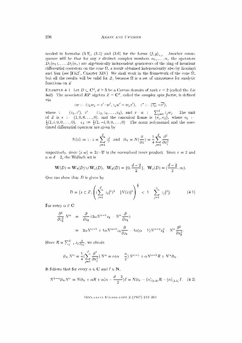
Example 4.1. Let D � C
d
, d � 3 be a Cartan domain of rank r = 2 (called the Lie
ball). The associated JB
�
-algebra Z = C
d
, called the complex spin factor, is de�ned
via
zw := (z
1
w
1
� z
0
� w
0
; z
1
w
0
+ w
1
z
0
); z
�
:= (z
1
;�z
0
);
where z = (z
1
; z
0
), z
0
= (z
2
; z
3
; : : : ; z
d
), and z � w :=
P
d
j=1
z
j
w
j
. The unit
of Z is e := (1; 0; 0; : : : ; 0), and the canonical frame is fe
1
; e
2
g, where e
1
:=
1
2
(1; i; 0; 0; : : : ; 0); e
2
:=
1
2
(1;�i; 0; 0; : : : ; 0). The norm polynomial and the asso-
ciated di�erential operator are given by
N(z) := z � z =
d
X
j=1
z
2
j
and @
N
= N(
@
@z
) =
1
4
d
X
j=1
@
2
@z
2
j
respectively, since (zjw) = 2z � w is the normalized inner product. Since r = 2 and
a = d� 2, the Wallach set is
W(D) =W
d
(D) [W
c
(D); W
d
(D) = f0;
d� 2
2
g; W
c
(D) = (
d� 2
2
;1):
One can show that D is given by
D = fz 2 Z;
0
@
(
d
X
j=1
jz
j
j
2
)
2
� jN(z)j
2
1
A
1
2
< 1�
n
X
j=1
jz
j
j
2
g: (4.1)
For every � 2 C
@
2
@z
2
k
N
�
=
@
@z
k
(2�N
��1
z
k
+N
�
@
@z
k
)
= 2�N
��1
+ 4�N
��1
z
k
@
@z
k
+ 4�(�� 1)N
��2
z
2
k
+N
�
@
2
@z
2
k
:
Since R =
P
d
j=1
z
j
@
@z
j
, we obtain
@
N
N
�
=
1
4
(
d
X
j=1
@
2
@z
2
j
)N
�
= �(� �
a
2
)N
��1
+ �N
��1
R+N
�
@
N
:
It follows that for every � 2 C and ` 2 N,
N
1��
@
N
N
�
= N@
N
+ �R + �(�+
d� 2
2
)I = N@
N
+ (�)
(1;0)
R+ (�)
(1;1)
I: (4.2)
Documenta Mathematica 2 (1997) 213{261
Invariant Inner Products 237
Since
D
`
(�) =
�
N
d
r
��
@
N
N
1+��
d
r
��
N
d
r
���1
@
N
N
2+��
d
r
�
� � �
�
N
d
r
+1�`��
@
N
N
`+��
d
r
�
;
we �nally obtain
D
`
(�) =
`
Y
j=1
(N@
N
+ (��
d
2
+ j)R+ (�� 1 + j)(� �
d
2
+ j)I): (4.3)
Note that the factors on the right hand sides of (4.2) and (4.3) commute, since they
are G()-invariant, and the entire ring of G()-invariant operators is commutative.
Also, the operators R and N@
N
are K-invariant. Hence the factors on the right hand
sides of (4.2) and (4.3) are multipliers of the Peter-Weyl decomposition of analytic
functions on D (see Corollary 2.1).
Consider a general Cartan domain of tube-type D � C
d
with rank r. Let be
the associated symmetric cone in the Euclidean Jordan algebra X and �x a frame
fe
1
; : : : ; e
r
g of pairwise orthogonal primitive idempotents in X , whose sum is the unit
element e. For 1 � � � r, let �
�
:= �
1
�
be the spherical polynomial associated with
the signature 1
�
:= (1; 1; : : : ; 1; 0; 0; : : : ; 0), where there are � \1"'s and r � � \0"'s.
Put also �
0
(z) � 1. Let f�
�
g
r
�=0
be the di�erential operators on de�ned via
(�
�
)f(a) := �
�
(
d
dx
)(f(P (a
1
2
)x))
jx=e
; (4.4)
where for b 2 X , P (b) is de�ned via (1.1). Recall that P (b) 2 G() for every b 2 ,
and that = fP (b)e; b 2 g since P (a
1
2
)e = a. Moreover, the L-invariance of the
�
�
's and the \polar decomposition" for imply that
(�
�
)f(a) := �
�
(
d
dx
)(f( (x)))
jx=e
; a 2 (4.5)
for every 2 G() for which (e) = a. This implies that the operators f�
�
g
r
�=0
are
G()-invariant, namely
�
�
(f � ) = (�
�
f) � ; 8 2 G(); 8f 2 C
1
():
We remark that (4.4) and (4.5) are equivalent to
�
�
e
hx;yi
jx=a
= �
�
(
�
(y)) e
ha;yi
= �
�
(P (a
1
2
)y) e
ha;yi
; a; y 2 ; (4.6)
where 2 G() � GL(X) satis�es (e) = a,
�
is the adjoint of with respect to
the inner product h�; �i on X , and �
�
di�erentiates the coordinate x. Notice also that
the operators �
�
can be written as
�
�
= c
m
K
m
(x;
@
@x
);
where m = (1; 1; : : : ; 1; 0; : : : ; 0) (� \ones" and r� � zeros), and c
m
is an appropriate
constant.
Documenta Mathematica 2 (1997) 213{261
238 Arazy and Upmeier
For � = 0; 1, r it is easy to compute �
�
. Clearly, �
0
= I . Since N is L-invariant,
�
r
= N . Using (4.6) and (1.3), we �nd that
�
r
= N @
N
:
Also, �
1
(x) =
1
r
tr(x) =
1
r
hx; ei. Indeed, using N
1
(x) = hx; e
1
i and the fact that L is
transitive on the frames, we get
�
1
(x) =
Z
L
h`x; e
1
i d` =
1
r
r
X
j=1
Z
L
h`x; e
j
i d`
=
1
r
Z
L
h`x; ei d` =
1
r
Z
L
hx; `ei d` =
1
r
hx; ei:
Using the fact that tr(P (a
1
2
)y) = hP (a
1
2
)y; ei = hy; P (a
1
2
)ei = hy; ai; 8a; y 2 , we
�nd that
�
1
=
1
r
R;
where Rf(x) :=
@
@t
f(tx)
jt=1
is the radial derivative.
Our main result in this section is the expansion of D
1
(�) = N
d
r
��
@
N
N
1+��
d
r
.
This result was obtained independently by A. Kor�anyi, see [FK2], Proposition
XIV.1.5.
Theorem 4.1 For every � 2 C,
D
1
(�) =
r
X
�=0
�
r
�
�
r
Y
j=�+1
(� � �
j
) �
�
: (4.7)
Proof: For x 2 , the function �! N(x)
�
is entire in �. Hence both sides of (4.7)
are entire in �, and it is therefore enough to prove (4.7) for � with <� < 0. Let
� = �
r
� �. Since <� > �
r
, we get for every x 2
N(x)
��
=
1
�
(�)
Z
e
�hx;ti
N(t)
�
d�
(t);
where d�
(t) := N(t)
�
d
r
dt is the G()-invariant measure on . Fix a; y 2 and put
f
y
(x) := e
hx;yi
. Then
(N
�+1
@
N
N
��
f
y
)(a)
=
N(a)
�+1
�
(�)
N(
d
dx
)
Z
e
hx;y�ti
N(t)
�
d�
(t)
jx=a
=
N(a)
�+1
�
(�)
Z
e
ha;y�ti
N(y � t)N(t)
�
d�
(t)
=
f
y
(a)
�
(�)
Z
e
�he;P (a
1
2
)ti
N(P (a
1
2
)(y � t))N(P (a
1
2
)t)
�
d�
(t):
Documenta Mathematica 2 (1997) 213{261
Invariant Inner Products 239
Letting b = P (a
1
2
)y, the substitution t := P (a
�
1
2
)P (b
1
2
)� gives
(N
�+1
@
N
N
��
f
y
)(a) =
f
y
(a)
�
(�)
N(y)
1+�
N(a)
1+�
Z
e
�hb;�i
N(e� �)N(�)
�
d�
(�):
Now, the well-known \binomial formula"
N(e+ x) =
r
X
�=0
�
r
�
�
�
�
(x); x 2 X (4.8)
(which follows from Theorem 1.2 and the knowledge of the norms of the �
�
's) and
the fact that for every s 2 C
r
and b 2
1
�
(s)
Z
e
�hb;�i
�
s
(�) d�
(�) = �
s
(b
�1
) (4.9)
(which follows from the analogous formula for the conical functions), imply
Z
e
�hb;�i
N(e� �)N(�)
�
d�(�) =
r
X
�=0
�
r
�
�
Z
e
�hb;�i
�
1
�
+�
(�) d�
(�)
=
r
X
�=0
�
r
�
�
�
(1
�
+ �) �
1
�
+�
(b
�1
) = N(b)
��
r
X
�=0
�
r
�
�
�
(1
�
+ �) �
�
(b
�1
):
We claim that for every b 2 and 1 � � � r,
�
�
(b
�1
) = �
r��
(b)N(b)
�1
: (4.10)
Indeed, using (4.8) we have N(e+ tb
�1
) =
P
r
�=0
�
r
�
�
�
�
(b
�1
) t
�
, as well as
N(e+ tb
�1
) = N(P (b
�
1
2
)(b+ te)) = N(b)
�1
t
r
N(e+ t
�1
b)
= N(b)
�1
t
r
r
X
k=0
�
r
k
�
�
k
(b) t
�k
:
Comparing the coe�cients of t
�
in the two expansions, we obtain (4.10). It follows
that
(N
�+1
@
N
N
��
f
y
)(a)
=
f
y
(a) N(y)
1+�
N(a)
1+�
�
(�) N(b)
1+�
r
X
�=0
(�1)
�
�
r
�
�
�
(1
�
+ �) �
r��
(b)
= f
y
(a)
r
X
�=0
(�1)
�
�
r
�
�
�
(1
�
+ �)
�
(�)
�
r��
(b)
= f
y
(a)
r
X
�=0
�
r
�
�
�
Y
j=1
(�
j
� �) �
r��
(P (a
1
2
)y):
Documenta Mathematica 2 (1997) 213{261
240 Arazy and Upmeier
Comparing this with (4.6), we conclude that
N
�+1
@
N
N
��
=
r
X
�=0
�
r
�
�
�
Y
j=1
(�
j
� �) �
r��
=
r
X
k=0
�
r
k
�
r�k
Y
j=1
(�
j
� �) �
k
:
Using the relations � = �
r
� � and
d
r
= 1 + �
r
, we obtain (4.7).
Remark: The \binomial formula" (4.8) yields that for every � = 1; 2; : : : ; r and every
x 2 X ,
�
�
(x) =
X
1�i
1
<i
2
<:::<i
�
�r
�
i
1
�
i
2
� � � �
i
�
=
�
r
�
�
= S
r;�
(�)=
�
r
�
�
;
where � = (�
1
; �
2
; : : : ; �
r
) is the sequence of eigenvalues of x, and S
r;�
is the elemen-
tary symmetric polynomial of degree � in r variables.
Combining the de�nition D
`
(�) =
Q
`�1
k=0
D
1
(�+ k) with Theorem 4.1, we obtain
Corollary 4.1 For every � 2 C and ` 2 N,
D
`
(�) =
`�1
Y
k=0
r
X
�=0
�
r
�
�
r
Y
j=�+1
(�+ k � �
j
) �
�
: (4.11)
For any signature m � 0 let �
m
be the di�erential operator associated with the
spherical polynomial �
m
via
(�
m
f)(a) := �
m
(
d
dx
) f(P (a
1
2
))
jx=e
; a 2 : (4.12)
Equivalently,
�
m
e
hx;yi
jx=a
= �
m
(P (a
1
2
)y) e
ha;yi
; a 2 : (4.13)
Again, one can replace in (4.12) and (4.13) P (a
1
2
) by any 2 G() satisfying (e) =
a. Hence the operators �
m
are G()-invariant, namely
�
m
(f � ) = (�
m
f) � ; 8 2 G():
Theorem 4.2 For every � 2 C and ` 2 N,
D
`
(�) =
X
m�0
(`)
�
(
d
r
+ `) �
(
d
r
� ��m
�
)
�
(
d
r
+ `�m
�
) �
(
d
r
� `� �)
d
m
(
d
r
)
m
�
m
(4.14)
= (
d
r
� �� `)
(`;:::;`)
X
m�0
(`)
(�`)
m
(�)
m
d
m
(
d
r
)
m
�
m
:
Here m
�
:= (m
r
;m
r�1
; : : : ;m
1
), d
m
= dim(P
m
), and the summation
P
m�0
(`)
extends over all m = (m
1
;m
2
; : : : ;m
r
) 2 N
r
with ` � m
1
� m
2
� : : : � m
r
� 0.
Documenta Mathematica 2 (1997) 213{261
Invariant Inner Products 241
Proof: The general binomial formula (1.15) and the relations
K
m
(x; e) =
�
m
k�
m
k
2
F
; k�
m
k
2
F
=
(
d
r
)
m
d
m
(see [FK2], Chapter XI) imply for ` 2 N and x 2 X
N(e+ x)
`
= c
X
m�0
(`)
d
m
(
d
r
)
`�m
�
(
d
r
)
m
�
m
(x); (4.15)
where c := (
d
r
)
(`;`;:::;`)
, and m
�
and
P
m�0
(`)
are as in Theorem 4.2. Indeed, by
(1.15),
N(e+ x)
`
=
X
m�0
(�`)
m
(�1)
jmj
d
m
(
d
r
)
m
�
m
(x):
From this (4.15) follows by the fact that (�`)
m
= 0 if m
1
> `, whereas in casem
1
� `,
(�`)
m
(�1)
jmj
=
(
d
r
)
(`;`;:::;`)
(
d
r
)
`�m
�
:
As in the proof of Theorem 4.1, it is enough to prove that for every � 2 C with
<� > �
r
and every ` 2 N,
N
�+`
@
`
N
N
��
= c
X
m�0
(`)
(�)
`�m
�
d
m
(
d
r
)
`�m
�
(
d
r
)
m
�
m
: (4.16)
From this one obtains (4.14) by the substitution � =
d
r
� `� �. To prove (4.16), �x
a; y 2 and let f
y
(x) := e
hx;yi
. Then
(N
�+`
@
`
N
N
��
f
y
)(a) =
N(a)
�+`
f
y
(a)
�
(�)
Z
e
�ha;ti
N(y � t)
`
N(t)
�
d�
(t)
=
N(b)
�+`
f
y
(a)
�
(�)
Z
e
�hb;ui
N(e� u)
`
N(u)
�
d�
(u);
by the substitutions b = P (a
1
2
)y and u = P (b
�
1
2
)P (a
1
2
)t. Using (4.15), (4.9), and
�
m
(x
�1
) = �
`�m
�
(x) N(x)
�`
(4.17)
(a consequence of [FK2], Proposition VII.1.5), we obtain
(N
�+`
@
`
N
N
��
f
y
)(a) = c
f
y
(a)
�
(�)
X
m�0
(`)
�
(m+ �) d
m
(
d
r
)
`�m
�
(
d
r
)
m
�
`�m
�
(P (a
1
2
)y):
With the change of variables n := `�m
�
, the fact that d
m
= d
n
(use (4.17) or the
general formula for d
m
in [U1]), the de�nition (4.12), and
(N
�+`
@
`
N
N
��
f
y
)(a) = c f
y
(a)
X
n�0
(`)
(�)
`�n
�
d
n
(
d
r
)
`�n
�
(
d
r
)
n
�
n
�
(P (a
1
2
)y);
we obtain (4.16).
Documenta Mathematica 2 (1997) 213{261
242 Arazy and Upmeier
Corollary 4.2 The operators f�
k
g
r
k=1
are algebraically independent generators of
the ring Di�()
G()
of G()-invariant di�erential operators on .
Proof: Comparing the two expansions (4.11) and (4.14) of D
`
(�), we see that
�
m
2 C[�
1
;�
2
; : : : ;�
r
]
for every signature m � 0. Since f�
m
g
m�0
is a basis for the space of spherical
polynomials, the one-to-one correspondence between spherical polynomials and the
elements of Di�()
G()
(see [FK2], Chapter XIV) implies that f�
m
g
m�0
is a basis
of Di�()
G()
. Thus Di�()
G()
= C[�
1
;�
2
; : : : ;�
r
]. Since the minimal number of
algebraic generators of Di�()
G()
is r = rank() [He], it follows that �
1
;�
2
; : : : ;�
r
are algebraically independent.
The divided di�erences of a C
1
-function f on R are de�ned by
f
[1]
(t
0
; t
1
) :=
f(t
0
)� f(t
1
)
t
0
� t
1
for t
0
6= t
1
, and f
[1]
(t
0
; t
0
) := f
0
(t
0
). The higher order divided di�erences of a smooth
enough function f are de�ned inductively by
f
[n]
(t
0
; t
1
; : : : ; t
n
) := g
[1]
(t
n�1
; t
n
);
where g(x) := f
[n�1]
(t
0
; t
1
; : : : ; t
n�2
; x). Then f
[n]
(t
0
; t
1
; : : : ; t
n
) is symmetric in
t
0
; t
1
; : : : ; t
n
, and
f
[n]
(t; t; : : : ; t) =
1
n!
d
n
dt
n
f(t):
Moreover, if f is analytic in a domain D � C, then
f
[n]
(t
0
; t
1
; : : : ; t
n
) =
1
2�i
Z
�
f(�)
Q
n
j=0
(� � t
j
)
d�
for all t
0
; t
1
; : : : ; t
n
2 D and every Jordan curve � in D whose interior contains
t
0
; t
1
; : : : ; t
n
and is contained in D. The divided di�erences of vector-valued maps
are de�ned in the same way and have analogous properties. For convenience we put
also f
[0]
(t) := f(t).
Theorem 4.3 Let �
1
; �
2
; : : : ; �
r
2 C be distinct. Then fD
1
(�
j
)g
r
j=1
are algebraically
independent generators of Di�()
G()
. Moreover, for ` = 1; 2; : : : ; r,
�
`
= D
[r�`]
1
(�
`
; �
`+1
; : : : ; �
r
)=
�
r
�
�
; (4.18)
where D
[r�`]
1
(�
`
; : : : ; �
r
) are the divided di�erences of order r� ` of D
1
(�), evaluated
at (�
`
; �
`+1
; : : : ; �
r
).
Documenta Mathematica 2 (1997) 213{261
Invariant Inner Products 243
Proof: Let h
k
(x) :=
�
r
`
�
Q
r
j=k+1
(x � �
j
), 0 � k � r. Then h
[m]
k
(x
0
; x
1
; : : : ; x
m
) � 0
whenever m > r � k, and h
[r�k]
k
(x
0
; x
1
; : : : ; x
r�k
) �
�
r
`
�
for all choices of
x
0
; x
1
; : : : ; x
r�k
. By Theorem 4.2, D
1
(�) =
P
r
k=0
h
k
(�)�
k
. Hence, for 1 � ` � r,
D
[r�`]
1
(�
`
; �
`+1
; : : : ; �
r
) =
`
X
k=0
h
[r�`]
k
(�
`
; �
`+1
; : : : ; �
r
) �
k
:
Solving this system of equations for the �
k
's, we see that Di�()
G()
=
C[�
1
;�
2
; : : : ;�
r
] coincides with the ring generated by the operators
fD
[r�`]
1
(�
`
; �
`+1
; : : : ; �
r
)g
r
`=1
. If the f�
j
g
r
j=1
are distinct, then
D
[r�`]
1
(�
`
; �
`+1
; : : : ; �
r
) 2 C[D
1
(�
1
); D
1
(�
2
); : : : ; D
1
(�
r
)]:
Hence,
Di�()
G()
= C[�
1
;�
2
; : : : ;�
r
] = C[D
1
(�
1
); D
1
(�
2
); : : : ; D
1
(�
r
)]:
The operators fD
1
(�
j
g
r
j=1
are algebraically independent, since Di�()
G()
cannot be
algebraically generated by less than r elements. If �
j
= �
j
for j = 1; 2; : : : ; r, then
h
[r�`]
k
(�
`
; : : : ; �
r
) = 0 for k < `. Thus, for ` = 1; 2; : : : ; r,
D
[r�`]
1
(�
`
; �
`+1
; : : : ; �
r
) = h
[r�`]
`
(�
`
; �
`+1
; : : : ; �
r
) �
`
=
�
r
`
�
�
`
:
Remark: The �rst statement in Theorem 4.3 was proved independently also by A.
Kor�anyi [FK2] and Z. Yan [Y1]. Our result is slightly stronger, giving the exact
formula (4.18).
Combining Theorems 3.2 and 4.2 (or, 4.1) we obtain integral formulas for the
invariant hermitian forms h�; �i
�;j
, � 2 P(D), 0 � j � q(�).
Corollary 4.3 Let � 2 P(D), ` 2 N and assume that � + ` �
d
r
= �
r
+ 1. Let
q = q(�), 0 � j � q, and � = q� j. Consider the G()-invariant di�erential operator
T
�;j
:=
X
m�0
(`)
c
m
(�; `)
d
m
(
d
r
)
m
�
m
; (4.19)
where is given by (3.4), and for every m � 0 with m
1
� `
c
m
(�; `) :=
1
�!
(
@
@�
)
`
�
(
d
r
+ `) �
(
d
r
� � �m
�
)
�
(
d
r
+ `�m
�
) �
(
d
r
� `� �)
!
j�=�
: (4.20)
Then T
�;j
is de�ned on all analytic functions on D, and for all f; g 2 H
�;j
hf; gi
�;j
= hT
�;j
f; gi
�+`
: (4.21)
In particular, if �+ ` > p� 1 or �+ ` =
d
r
then we have
hf; gi
�;j
=
Z
D
(T
�;j
f)(z) g(z) d�
�+`
(z) and hf; gi
�;j
=
Z
S
(T
�;j
f)(�) g(�) d�(�)
(4.22)
respectively.
Documenta Mathematica 2 (1997) 213{261
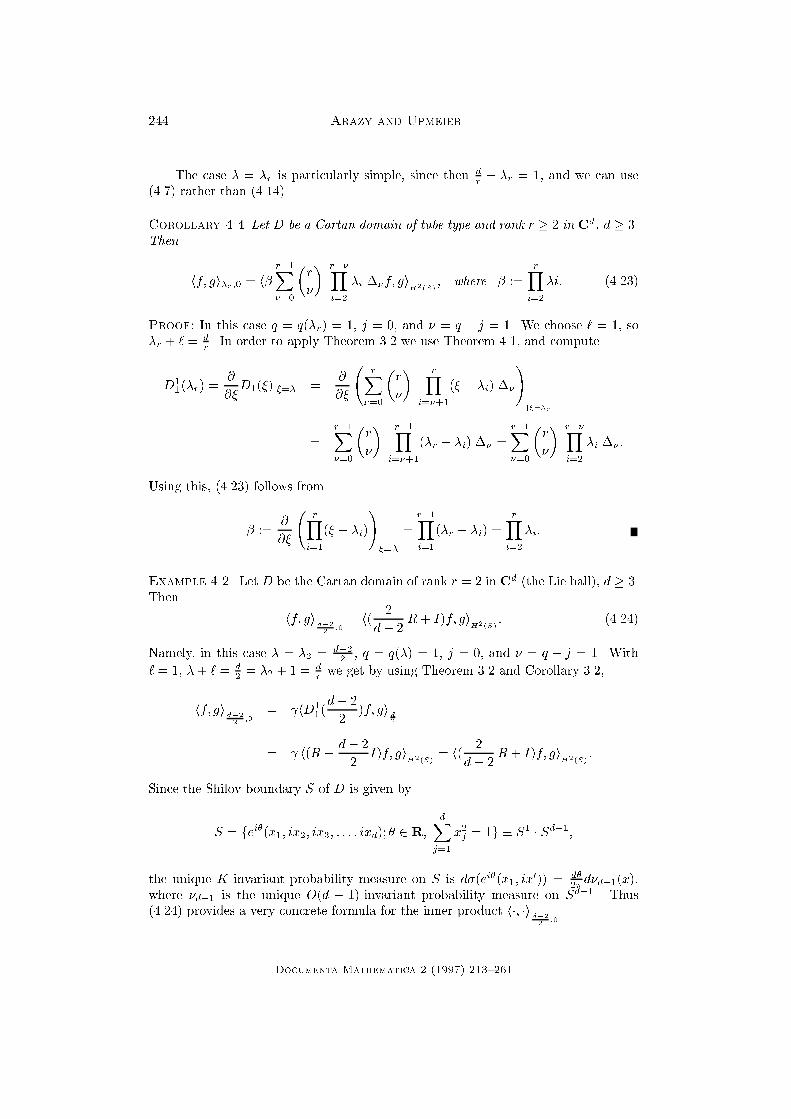
244 Arazy and Upmeier
The case � = �
r
is particularly simple, since then
d
r
� �
r
= 1, and we can use
(4.7) rather than (4.14).
Corollary 4.4 Let D be a Cartan domain of tube type and rank r � 2 in C
d
, d � 3.
Then
hf; gi
�
r
;0
= h�
r�1
X
�=0
�
r
�
�
r��
Y
i=2
�
i
�
�
f; gi
H
2
(S)
; where � :=
r
Y
i=2
�i: (4.23)
Proof: In this case q = q(�
r
) = 1, j = 0, and � = q � j = 1. We choose ` = 1, so
�
r
+ ` =
d
r
. In order to apply Theorem 3.2 we use Theorem 4.1, and compute
D
1
1
(�
r
) =
@
@�
D
1
(�)
j�=�
=
@
@�
r
X
�=0
�
r
�
�
r
Y
i=�+1
(� � �
i
) �
�
!
j�=�
r
=
r�1
X
�=0
�
r
�
�
r�1
Y
i=�+1
(�
r
� �
i
) �
�
=
r�1
X
�=0
�
r
�
�
r��
Y
i=2
�
i
�
�
:
Using this, (4.23) follows from
� :=
@
@�
r
Y
i=1
(� � �
i
)
!
�=�
=
r�1
Y
i=1
(�
r
� �
i
) =
r
Y
i=2
�
i
:
Example 4.2. Let D be the Cartan domain of rank r = 2 in C
d
(the Lie ball), d � 3.
Then
hf; gi
d�2
2
;0
= h(
2
d� 2
R+ I)f; gi
H
2
(S)
: (4.24)
Namely, in this case � = �
2
=
d�2
2
, q = q(�) = 1, j = 0, and � = q � j = 1. With
` = 1, �+ ` =
d
2
= �
2
+ 1 =
d
r
we get by using Theorem 3.2 and Corollary 3.2,
hf; gi
d�2
2
;0
= hD
1
1
(
d� 2
2
)f; gi
d
2
= h(R +
d� 2
2
I)f; gi
H
2
(S)
= h(
2
d� 2
R+ I)f; gi
H
2
(S)
:
Since the Shilov boundary S of D is given by
S = fe
i�
(x
1
; ix
2
; ix
3
; : : : ; ix
d
); � 2 R;
d
X
j=1
x
2
j
= 1g � S
1
� S
d�1
;
the unique K-invariant probability measure on S is d�(e
i�
(x
1
; ix
0
)) =
d�
2�
d�
d�1
(x);
where �
d�1
is the unique O(d � 1)-invariant probability measure on S
d�1
. Thus
(4.24) provides a very concrete formula for the inner product h�; �i
d�2
2
;0
.
Documenta Mathematica 2 (1997) 213{261
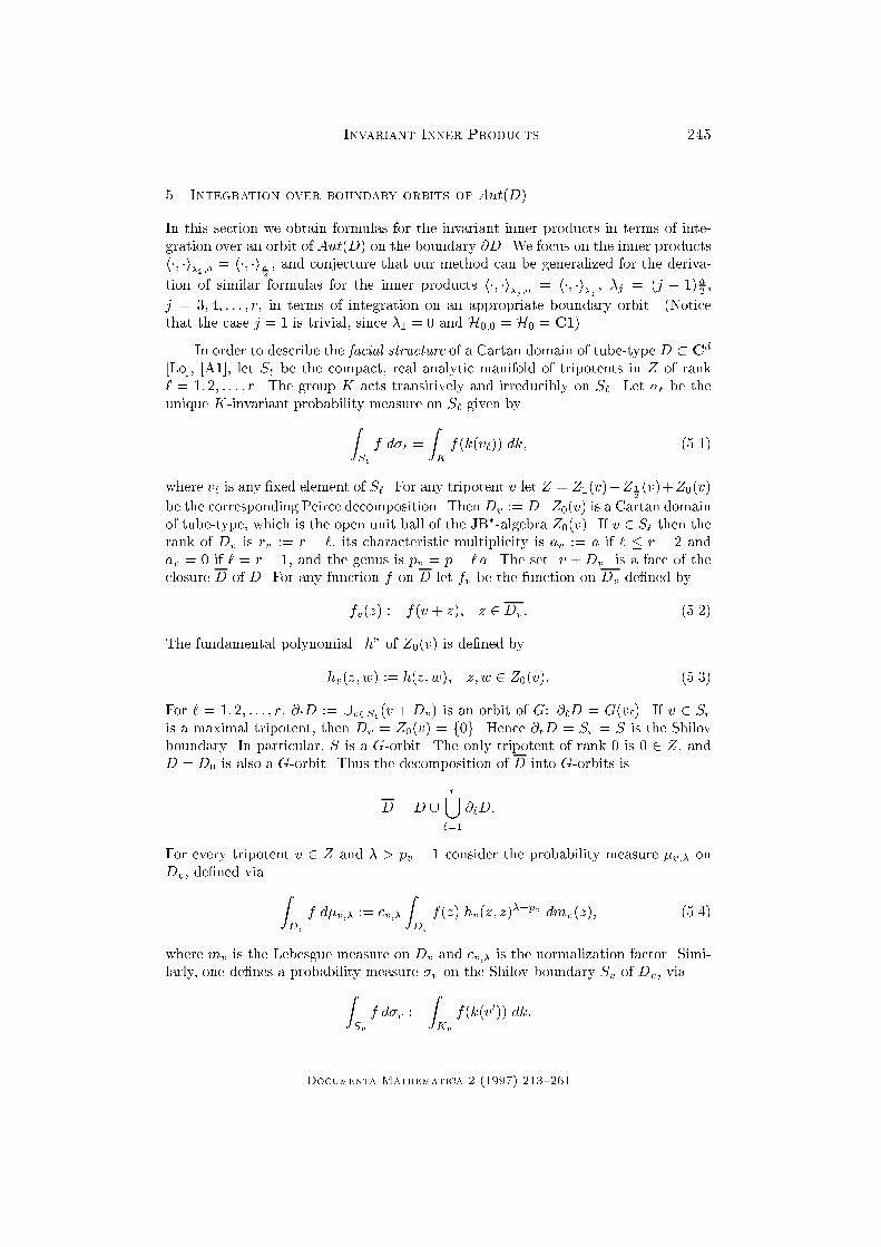
Invariant Inner Products 245
5 Integration over boundary orbits of Aut(D)
In this section we obtain formulas for the invariant inner products in terms of inte-
gration over an orbit of Aut(D) on the boundary @D. We focus on the inner products
h�; �i
�
2
;0
= h�; �i
a
2
, and conjecture that our method can be generalized for the deriva-
tion of similar formulas for the inner products h�; �i
�
j
;0
= h�; �i
�
j
, �
j
= (j � 1)
a
2
,
j = 3; 4; : : : ; r, in terms of integration on an appropriate boundary orbit. (Notice
that the case j = 1 is trivial, since �
1
= 0 and H
0;0
= H
0
= C1).
In order to describe the facial structure of a Cartan domain of tube-type D � C
d
[Lo], [A1], let S
`
be the compact, real analytic manifold of tripotents in Z of rank
` = 1; 2; : : : ; r. The group K acts transitively and irreducibly on S
`
. Let �
`
be the
unique K-invariant probability measure on S
`
given by
Z
S
`
f d�
`
=
Z
K
f(k(v
`
)) dk; (5.1)
where v
`
is any �xed element of S
`
. For any tripotent v let Z = Z
1
(v)+Z
1
2
(v)+Z
0
(v)
be the corresponding Peirce decomposition. Then D
v
:= D\Z
0
(v) is a Cartan domain
of tube-type, which is the open unit ball of the JB
�
-algebra Z
0
(v). If v 2 S
`
then the
rank of D
v
is r
v
:= r � `, its characteristic multiplicity is a
v
:= a if ` � r � 2 and
a
v
= 0 if ` = r � 1, and the genus is p
v
= p � ` a. The set v +D
v
is a face of the
closure D of D. For any function f on D let f
v
be the function on D
v
de�ned by
f
v
(z) := f(v + z); z 2 D
v
: (5.2)
The fundamental polynomial \h" of Z
0
(v) is de�ned by
h
v
(z; w) := h(z; w); z; w 2 Z
0
(v): (5.3)
For ` = 1; 2; : : : ; r, @
`
D := [
v2S
`
(v +D
v
) is an orbit of G: @
`
D = G(v
`
). If v 2 S
r
is a maximal tripotent, then D
v
= Z
0
(v) = f0g. Hence @
r
D = S
r
= S is the Shilov
boundary. In particular, S is a G-orbit. The only tripotent of rank 0 is 0 2 Z, and
D = D
0
is also a G-orbit. Thus the decomposition of D into G-orbits is
D = D [
r
[
`=1
@
`
D:
For every tripotent v 2 Z and � > p
v
� 1 consider the probability measure �
v;�
on
D
v
, de�ned via
Z
D
v
f d�
v;�
:= c
v;�
Z
D
v
f(z) h
v
(z; z)
��p
v
dm
v
(z); (5.4)
where m
v
is the Lebesgue measure on D
v
and c
v;�
is the normalization factor. Simi-
larly, one de�nes a probability measure �
v
on the Shilov boundary S
v
of D
v
, via
Z
S
v
f d�
v
:=
Z
K
v
f(k(v
0
)) dk;
Documenta Mathematica 2 (1997) 213{261
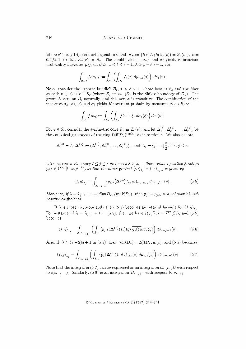
246 Arazy and Upmeier
where v
0
is any tripotent orthogonal to v and K
v
:= fk 2 K; k(Z
�
(v)) = Z
�
(v)g; � =
0; 1=2; 1, so that K
v
(v
0
) = S
v
. The combination of �
v;�
and �
`
yields K-invariant
probability measures �
`;�
on @
`
D, 1 � ` � r � 1, � > p� ` a� 1, via
Z
@
`
D
fd�
`;�
:=
Z
S
`
�
Z
D
v
f
v
(z) d�
v;�
(z)
�
d�
`
(v):
Next, consider the \sphere bundle" B
`
, 1 � ` � r, whose base is S
`
and the �ber
at each v 2 S
`
is v + S
v
(where S
v
:= @
r�`
D
v
is the Shilov boundary of D
v
). The
group K acts on B
`
naturally, and this action is transitive. The combination of the
measures �
v
, v 2 S
`
and �
`
yields K-invariant probability measures �
`
on B
`
via
Z
B
`
f d�
`
:=
Z
S
`
�
Z
S
v
f(v + �) d�
v
(�)
�
d�
`
(v):
For v 2 S
`
, consider the symmetric cone
v
in Z
0
(v), and let �
(v)
1
;�
(v)
2
; : : : ;�
(v)
r�`
be
the canonical generators of the ring Di�(
v
)
G(
v
)
as in section 4. We also denote
�
(v)
0
= I; �
(v)
:= (�
(v)
1
;�
(v)
2
; : : : ;�
(v)
r�`
); and �
j
= (j � 1)
a
2
; 0 � j � r:
Conjecture: For every 2 � j � r and every � > �
j�1
there exists a positive function
p
j;�
2 C
1
([0;1)
j�1
), so that the inner product h�; �i
�
j
= h�; �i
�
j
;0
is given by
hf; gi
�
j
=
Z
S
r�j+1
hp
j;�
(�
(v)
)f
v
; g
v
i
H
�
(D
v
)
d�
r�j+1
(v): (5.5)
Moreover, if � = �
j�1
+ 1 = dim(D
v
)=rank(D
v
), then p
j
:= p
j;�
is a polynomial with
positive coe�cients.
If � is chosen appropriately then (5.5) becomes an integral formula for hf; gi
�
j
.
For instance, if � = �
j�1
+ 1 in (5.5), then we have H
�
(D
v
) = H
2
(S
v
), and (5.5)
becomes
hf; gi
�
j
=
Z
S
r�j+1
�
Z
S
v
(p
j;�
(�
(v)
)f
v
)(�) g
v
(�)d�
v
(�)
�
d�
r�j+1
(v): (5.6)
Also, if � > (j � 2)a+ 1 in (5.5) then H
�
(D
v
) = L
2
a
(D
v
; �
v;�
), and (5.5) becomes
hf; gi
�
j
=
Z
S
r�j+1
�
Z
D
v
(p
j
(�
(v)
)f
v
)(z) g
v
(z) d�
v;�
(z)
�
d�
r�j+1
(v): (5.7)
Note that the integral in (5.7) can be expressed as an integral on @
r�j+1
D with respect
to d�
r�j+1;�
. Similarly, (5.6) is an integral on B
r�j+1
with respect to �
r�j+1
.
Documenta Mathematica 2 (1997) 213{261
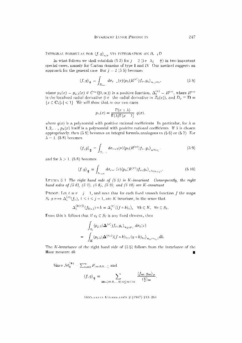
Invariant Inner Products 247
Integral formulas for hf; gi
a=2
via integration on @
r�1
D
In what follows we shall establish (5.5) for j = 2 (i.e. �
2
=
a
2
) in two important
special cases, namely for Cartan domains of type I and IV. Our method suggests an
approach for the general case. For j = 2 (5.5) becomes
hf; gi
a
2
=
Z
S
r�1
d�
r�1
(v)hp
�
(R
(v)
)f
v
; g
v
i
H
�
(D)
; (5.8)
where p
�
(x) = p
2;�
(x) 2 C
1
([0;1)) is a positive function, �
(v)
1
= R
(v)
, where R
(v)
is the localized radial derivative (i.e. the radial derivative in Z
0
(v)), and D
v
� D =
fz 2 C; jzj < 1g. We will show that in our two cases
p
�
(x) =
�(x+ �)
�(�)�(x + 1)
q(x);
where q(x) is a polynomial with positive rational coe�cients. In particular, for � =
1; 2; : : :, p
�
(x) itself is a polynomial with positive rational coe�cients. If � is chosen
appropriately, then (5.8) becomes an integral formula analogous to (5.6) or (5.7). For
� = 1, (5.8) becomes
hf; gi
a
2
=
Z
S
r�1
d�
r�1
(v)hp
1
(R
(v)
)f
v
; g
v
i
H
2
(T)
; (5.9)
and for � > 1, (5.8) becomes
hf; gi
a
2
=
Z
S
r�1
d�
r�1
(v)hp
�
(R
(v)
)f
v
; g
v
i
L
2
(D;�
�
)
: (5.10)
Lemma 5.1 The right hand side of (5.5) is K-invariant. Consequently, the right
hand sides of (5.6), (5.7), (5.8), (5.9), and (5.10) are K-invariant.
Proof: Let ` = r � j + 1, and note that for each �xed smooth function f the maps
S
`
3 v 7! �
(v)
i
(f
v
), 1 � i � j � 1, are K-invariant, in the sense that
�
(k(v))
i
(f
k(v)
) � k = �
(v)
i
((f � k)
v
); 8k 2 K; 8v 2 S
`
:
From this it follows that if v
`
2 S
`
is any �xed element, then
Z
S
`
hp
j;�
(�
(v)
)f
v
; g
v
i
H
�
(D
v
)
d�
`
(v)
=
Z
K
hp
j;�
(�
(v
`
)
)(f � k)
v
`
; (g � k)
v
`
i
H
�
(D
v
`
)
dk:
The K-invariance of the right hand side of (5.5) follows from the invariance of the
Haar measure dk.
Since M
(
a
2
)
0
=
P
1
m=0
P
(m;0;0;:::)
and
hf; gi
a
2
=
X
m=(m;0;:::;0);0�m<1
hf
m
; g
m
i
F
(
a
2
)
m
;
Documenta Mathematica 2 (1997) 213{261
248 Arazy and Upmeier
in order to establish (5.8) it is enough, by the K-invariance of both sides, to �nd
positive functions p
�
(x) 2 C
1
([0;1)) so that (5.8) holds for the functions f(z) =
g(z) = N
m
1
(z), m � 0. This is equivalent to
Z
S
r�1
d�
r�1
(v)hp
�
(R
(v)
)(N
m
1
)
v
; (N
m
1
)
v
i
H
�
(D)
=
m!
(
a
2
)
m
: (5.11)
Fix a frame e
1
; e
2
; : : : ; e
r
in Z. Then N
1
(z) = (z; e
1
), where (�; �) is the unique K-
invariant inner product on Z for which (v; v) = 1 for every minimal tripotent v. Let
e
0
:= e
2
+ e
3
+ : : :+ e
r
. Then for z = k(�e
1
+ e
0
) with k 2 K and � 2 T, we have
N
m
1
(z) = (�k(e
1
) + k(e
0
); e
1
)
m
=
m
X
`=0
�
m
`
�
(k(e
1
); e
1
)
`
(k(e
0
); e
1
)
m�`
�
`
:
Thus, for v = k(e
0
), m � 0 and any continuous function f we have
(f(R
(v)
)N
m
1
)(z) =
m
X
`=0
�
m
`
�
(k(e
1
); e
1
)
`
(k(e
0
); e
1
)
m�`
f(`) �
`
:
Let us de�ne
J
m;`
:=
Z
K
j(k(e
1
); e
1
)j
2`
j(k(e
0
); e
1
)j
2(m�`)
dk; 0 � ` � m <1: (5.12)
It follows that the function p
�
should satisfy
Z
S
r�1
d�
r�1
(v) hp
�
(R
(v)
)(N
m
1
)
v
; (N
m
1
)
v
i
H
�
(D)
=
m
X
`=0
J
m;`
�
m
`
�
2
`!
(�)
`
p
�
(`):
Thus (5.11) becomes
m
X
`=0
J
m;`
�
m
`
�
2
q
`
=
m!
(
a
2
)
m
; m = 0; 1; 2; : : : ; (5.13)
where the numbers
q
`
:=
`!
(�)
`
p
�
(`); ` = 0; 1; 2; : : : (5.14)
do not depend on �. The in�nite system of linear equations (5.13) in the unknowns
fq
`
g
1
`=0
corresponds to the lower triangular matrix A = (a
m;`
)
1
m;`=0
, where a
m;`
=
J
m;`
�
m
`
�
2
for m � `, and a
m;`
= 0 for m < `. Since a
m;m
> 0 for m = 0; 1; 2; : : :,
there exists a unique solution fq
`
g
1
`=0
to (5.13). There are many smooth functions
which interpolate the values fq
`
g
1
`=0
. We will show that q
`
> 0 for every ` � 0, and
prove that fq
`
g
1
`=0
can be interpolated by a polynomial of degree r � 1 with positive
coe�cients. For Cartan domains of type I and IV, we will solve the system (5.13) by
calculating explicitly the numbers J
m;`
and applying powers of the di�erence operator
�(f)(t) := f(t)� f(t� 1); t 2 R:
Documenta Mathematica 2 (1997) 213{261
Invariant Inner Products 249
If f is de�ned only on [0;1) then we de�ne �(f) := �(F ), where F (t) := f(t) for
0 � t and F (t) = 0 for 0 > t. Similarly, � can be de�ned on two-sided sequences (i.e.
on functions on Z) or on sequences (i.e. functions on N). The powers of � are de�ned
inductively by �
n+1
:= � � �
n
.
Case 1: Cartan domains of type I. Let D = D(I
r;r
) := fz 2M
r;r
(C); kzk < 1g.
The rank of D is r, the dimension is d = r
2
, the genus is p = 2r, and the characteristic
multiplicity is a = 2. To every k 2 K there correspond u;w 2 U(r) (the unitary group)
so that det(u) = det(w), and
k(z) = uzw
�
; z 2 D: (5.15)
Thus
R
K
f(k(z)) dk =
R
U(r)
R
U(r)
f(uzw
�
) du dw, where dk is the Haar measure of
K. Choose the canonical frame of matrix units e
j
:= e
j;j
; j = 1; 2; : : : ; r, and denote
e =
P
r
j=1
e
j
and e
0
:= e� e
1
=
P
r
j=2
e
j
.
Proposition 5.1 Let D = D(I
r;r
). Then for every integers m; ` with 0 � ` � m <
1, we have
J
m;`
=
(r � 1) (` !)
2
(m� `)! (m� `+ r � 2)!
(r)
m
(m+ r � 1)!
: (5.16)
Proof: Let k 2 K be given by (5.15). Then (k(e
1
); e
1
) = u
1;1
w
1;1
and (k(e
0
); e
1
) =
P
r
j=2
u
1;j
w
1;j
. Thus, for 0 � ` � m <1,
J
m;`
=
Z
U(r)
Z
U(r)
ju
1;1
j
2`
jw
1;1
j
2`
j
r
X
j=2
u
1;j
w
1;j
j
2(m�`)
du dw:
This integral can be written as an integral on the product of the unit spheres @B
r
�
C
r
with respect to the U(r)-invariant probability measure �:
J
m;`
=
Z
@B
r
Z
@B
r
j�
`
1
j
2
j�
`
1
j
2
j(�
0
; �
0
)j
2(m�`)
d�(�) d�(�);
where �
0
:= (�
2
; : : : ; �
r
) and �
0
:= (�
2
; : : : ; �
r
). Now, by the U(r)-invariance,
Z
@B
r
j�
`
1
j
2
j(�
0
; �
0
)j
2(m�`)
d�(�)
= k�
0
k
2(m�`)
Z
@B
r
j�
`
1
j
2
j�
m�`
2
j
2
d�(�)
= k�
0
k
2(m�`)
k�
`
1
�
m�`
2
k
2
H
r
(D)
= k�
0
k
2(m�`)
`!(m� `)!
(r)
m
:
It follows by using [Ru], 1.4.5, that
J
m;`
=
`!(m� `)!
(r)
m
Z
@B
r
j�
`
1
j
2
(1� j�
1
j
2
)
m�`
d�(�)
=
`!(m� `)!
(r)
m
(r � 1)
Z
1
0
t
`
(1� t)
m�`+r�2
dt
Documenta Mathematica 2 (1997) 213{261
250 Arazy and Upmeier
=
`!(m� `)!
(r)
m
(r � 1)B(`+ 1;m� `+ r � 1)
=
(r � 1)(`!)
2
(m� `)!(m� `+ r � 2)!
(r)
m
(m+ r � 1)!
:
Corollary 5.1 For D = D(I
r;r
) the system of equations (5.13) is equivalent to the
system
m
X
`=0
(m� `+ r � 2)!
(m� `)!
q
`
= (r � 2)!
�
m+ r � 1
r � 1
�
2
; m = 0; 1; 2; : : : : (5.17)
Proposition 5.2 For every r � 2 there exists a polynomial q(x) = q
r
(x) of degree
r � 1 with positive rational coe�cients, so that q(`) = q
`
for ` = 0; 1; 2; : : : , where
fq
`
g
1
`=0
is the unique solution of (5.17).
For small values of r it is easy to solve (5.17) explicitly by applying powers of �. Thus,
q
2
(x) = 2x+ 1; q
3
(x) = 3x
2
+ 3x+ 1; and q
4
(x) =
1
3
(10x
3
+ 15x
2
+ 11x+ 3):
The proof in the general case requires more preparation. De�ne
f
n
(x) := (x+ 1)
n
=
n
Y
j=1
(x + j); n � 1; and g
n
(x) :=
n
Y
j=0
(x+ j)
2
; n � 0: (5.18)
Then g
n
(x+ 1) = f
n+1
(x)
2
, and
(�
k
f
n
)(x) = n(n� 1) � � � (n� k + 1) f
n�k
(x); k � 0; (5.19)
where � is de�ned by �(f)(x) := f(x) � f(x � 1). Indeed, (5.19) is trivial for k = 0.
For k = 1 and all n we have
�(f
n
)(x) =
n
Y
j=1
(x+ j)�
n
Y
j=1
(x + j � 1) =
n�1
Y
j=1
(x+ j) (x+ n� x) = n f
n�1
(x):
Assuming (5.19) for k, let n > k and compute �
k+1
(f
n
)(x) = n(n � 1) � � � (n � k +
1) �(f
n�k
)(x) = n(n� 1) � � � (n� k + 1)(n� k)f
n�k�1
(x): This establishes (5.19).
Next, de�ne an operator �, analogous to �, via
(�f)(x) := f(x) + f(x� 1); x 2 R:
Clearly, �� = ��, and both � and � commute with all the translation operators
(�
c
f)(x) := f(x+ c):
Denote by P
+
the set of polynomials in one variable with non-negative coe�cients.
Documenta Mathematica 2 (1997) 213{261
Invariant Inner Products 251
Lemma 5.2 Let f(x) be a polynomial and let n;m 2 N. If �
n
f 2 P
+
, then
�
n+j
�
m=2
f 2 P
+
for every integer 0 � j � m.
Proof: Since � commutes with translations, we may assume that n = 0 and m = 1.
It is therefore enough to check that ��
1=2
x
k
2 P
+
for every k 2 N. This follows from
the binomial expansion:
��
1=2
x
k
= (x+
1
2
)
k
� (x �
1
2
)
k
=
[
k�1
2
]
X
j=0
�
k
2j + 1
�
2
�2j
x
k�2j�1
:
Lemma 5.3 Let f(x) be a polynomial and let n 2 N. Assume that �
j
�
n�j
f 2
P
+
for every 0 � j � n. Then �
j
�
n�j
�
(x+ c)
k
f(x)
�
2 P
+
for every k 2 N,
c �
n
2
and 0 � j � n.
Proof: Again, since � and � commute with translations, it is enough to assume that
k = 1. We shall prove the assertion by induction on n. The case n = 0 is trivial since
P
+
is closed under sums and products. Assume that n > 0 and that the assertion
holds for n� 1. A computation yields
�
�
(x +
n
2
)f(x)
�
= (x +
n� 1
2
)(�f)(x) +
1
2
(�f)(x) (5.20)
and
�
�
(x+
n
2
)f(x)
�
= (x+
n� 1
2
)(�f)(x) +
1
2
(�f)(x): (5.21)
If 0 < j � n then using (5.20) we get
�
j
�
n�j
�
(x +
n
2
)f(x)
�
= �
j�1
�
(n�1)�(j�1)
�
(x+
n� 1
2
)(�f)(x) +
1
2
(�f)(x)
�
:
By assumption,
�
j�1
�
(n�1)�(j�1)
�f = �
j�1
�
n�(j�1)
f 2 P
+
; for 0 < j � n:
Similarly,
�
j�1
�
(n�1)�(j�1)
�f = �
j
�
n�j
f 2 P
+
for 0 < j � n:
Thus, by the induction hypothesis on n� 1,
�
j�1
�
(n�1)�(j�1)
�
(x+
n� 1
2
)�f(x)
�
2 P
+
; for 0 < j � n:
Next, using (5.21) we get
�
n
�
(x+
n
2
)f(x)
�
= �
n�1
�
(x+
n� 1
2
)�f(x) +
1
2
�f(x)
�
:
By assumption, �
n�1
�f(x) 2 P
+
and �
`
�
n�1�`
�f(x) 2 P
+
for 0 � ` � n� 1. Thus,
by the induction hypothesis, �
`
�
n�1�`
�
(x+
n�1
2
)�f(x)
�
2 P
+
for 0 � ` � n� 1, and
in particular �
n�1
�
(x+
n�1
2
)�f(x)
�
2 P
+
. It follows that �
n
�
(x +
n
2
)f(x)
�
2 P
+
.
This completes the induction step.
Documenta Mathematica 2 (1997) 213{261
252 Arazy and Upmeier
Lemma 5.4 Let g
n
(x) be the polynomial de�ned by (5.18). Then �
i
�
j
g
n
2 P
+
when-
ever i+ j � n.
Proof: We proceed by induction on n. The case n = 0 is trivial, since g
0
(x) =
x
2
2 P
+
. Assume that n > 0 and that �
i
�
j
g
n�1
2 P
+
whenever i + j � n � 1. A
computation yields
�g
n
(x) = 2(n+ 1)(x+
n� 1
2
) g
n�1
(x) (5.22)
and
�g
n
(x) = 2
�
(x+
n� 1
2
)
2
+ (
n+ 1
2
)
2
�
g
n�1
(x): (5.23)
Now assume i+ j � n. If i > 0, (5.22) yields
�
i
�
j
g
n
(x) = �
i�1
�
j
(�g
n
(x)) = 2(n+ 1)�
i�1
�
j
�
(x +
n� 1
2
)g
n�1
(x)
�
;
and by induction hypothesis and Lemma 5.3
�
i�1
�
j
�
(x +
n� 1
2
)g
n�1
(x)
�
2 P
+
;
so that �
i
�
j
g
n
2 P
+
. If i = 0 and 0 � j � n, then (5.23) implies
�
j
g
n
(x) = �
j�1
(�g
n
(x)) = 2�
j�1
��
(x+
n� 1
2
)
2
+ (
n+ 1
2
)
2
�
g
n�1
(x)
�
:
The polynomial �
j�1
g
n�1
belongs to P
+
by the induction hypothesis. Also, the
induction hypothesis (�
i
�
j�1
g
n�1
2 P
+
whenever i + j � n) and Lemma 5.3 imply
that
�
i
�
j�1
�
(x +
n� 1
2
)g
n�1
(x)
�
2 P
+
whenever i+ j � n:
In particular, �
j�1
�
(x+
n�1
2
)g
n�1
(x)
�
2 P
+
. Hence �
j
g
n
2 P
+
8 0 � j � n.
Corollary 5.2 (i) �
j
g
n
2 P
+
for all j; n 2 N satisfying 0 � j � n.
(ii) �
j
�
(x+
m
2
)g
n
(x)
�
2 P
+
for all j; n;m 2 N satisfying 0 � j � n+m.
(iii) �
j
f
n
(x)
2
2 P
+
for all j; n 2 N satisfying 0 � j � n+ 1.
Proof: (i) is a special case of Lemma 5.4, and (ii) follows by (i) and Lemma 5.2.
Since f
n
(x)
2
= g
n�1
(x+ 1), (iii) follows from Lemma 5.2 with m = 2.
Remark The result in part (iii) of Corollary 5.2 is best possible in the sense that
�
n+2
(f
2
n
)
2
) need not be in P
+
. Indeed, �
6
(f
2
4
)
2
) is not in P
+
.
Documenta Mathematica 2 (1997) 213{261
Invariant Inner Products 253
Proof of Proposition 5.2: In terms of the polynomials (5.18), the system of
equations (5.17) with unknowns q
`
has the form
m
X
`=0
f
r�2
(m� `) q
`
=
f
r�1
(m)
2
(r � 1) (r � 1)!
; m � 0: (5.24)
Applying powers of the operator � with respect to the variable m and using (5.19),
we get by induction on k that
�
k
m
X
`=0
f
r�2
(m� `) q
`
!
= (r � 2)(r � 3) � � � (r � k � 1)
m
X
`=0
f
r�2�k
(m� `) q
`
for 0 � k � r � 2 (here f
0
(x) � 1). From this it follows that
�
r�1
m
X
`=0
f
r�2
(m� `) q
`
!
= (r � 2)! q
m
; m � 0:
Applying �
r�1
to both sides of (5.24), Corollary 5.2 (iii) implies that there exists
a polynomial q(x) of degree r � 1 with positive rational coe�cients so that q
m
=
q(m); 8m � 0.
Theorem 5.1 Let D = D(I
r;r
). Then for every f; g 2 H
a
2
(D) and � > 0 we have
hf; gi
a
2
=
Z
S
r�1
d�
r�1
(v)hp
�
(R
(v)
)f
v
; g
v
i
H
�
(D)
;
where p
�
(x) := �(x+�) �(�)
�1
�(x+1)
�1
q(x), and q(x) is the polynomial of degree
r � 1 with positive rational coe�cients as in Proposition 5.2.
Case 2: Cartan domains of type IV. Let D � C
d
, d � 3, be the Cartan domain
of rank r = 2 (see Examples 4.1 and 4.2), and �x a frame fe
1
; e
2
g. Since a = d � 2,
(5.13) becomes
m
X
`=0
�
m
`
�
2
J
m;`
q
`
=
m!
(
a
2
� 1)
m
; m � 0; (5.25)
where for 0 � ` � m
J
m;`
=
Z
K
j(k(e
1
); e
1
)j
2`
j(k(e
2
); e
1
)j
2(m�`)
dk:
Without computing the numbers J
m;`
explicitly we show that
J
m;`
= J
m;m�`
; 0 � ` � m: (5.26)
Indeed, let k
0
2 K satisfy k
0
(e
1
) = e
2
and k
0
(e
2
) = e
1
. Then, by invariance of the
Haar measure dk,
J
m;`
=
Z
K
j(k(k
0
(e
1
)); e
1
)j
2`
j(k(k
0
(e
2
)); e
1
)j
2(m�`)
dk
=
Z
K
j(k(e
2
); e
1
)j
2`
j(k(e
1
); e
1
)j
2(m�`)
dk = J
m;m�`
:
Documenta Mathematica 2 (1997) 213{261
254 Arazy and Upmeier
Theorem 5.2 The polynomial
q(x) =
4
a
x+ 1 =
4
d� 2
x+ 1
satis�es q(`) = q
`
for every ` � 0, where fq
`
g
1
`=0
is the unique solution of (5.25).
Therefore, for every � > 0 and every f; g 2 H
a
2
(D),
hf; gi
a
2
=
Z
S
1
hp
�
(R
(v)
)f
v
; g
v
i
H
�
(D
v
)
d�
1
(v);
where the functions p
�
, 0 < � <1, are given by
p
�
(x) =
�(x+ �)
�(�) �(x + 1)
(
4
a
x+ 1): (5.27)
In particular, for � = 1; 2; : : : p
�
is a polynomial of degree � with positive rational
coe�cients.
Proof: We claim �rst that
m
X
`=0
�
m
`
�
2
J
m;`
=
m!
(
d
2
)
m
; m � 0: (5.28)
Indeed, it is clear that
m
X
`=0
�
m
`
�
2
J
m;`
=
Z
K
�
Z
T
j(k(e
it
e
1
+ e
2
); e
1
)
m
j
2
dt
2�
�
dk:
Interchanging the order of integration and using the transitivity of K on the frames,
we get
m
X
`=0
�
m
`
�
2
J
m;`
=
Z
K
j(k(e); e
1
)
m
j
2
dk = kN
m
1
k
2
H
2
(D)
=
m!
(
d
2
)
m
; m � 0;
by using the well-known fact that k(�; z)
m
k
2
F
= m!(z; z)
m
for every z 2 Z and m � 0.
Using (5.26) and (5.28) we see that
m
X
`=0
`
�
m
`
�
2
J
m;`
=
m
X
`=0
(m� `)
�
m
m� `
�
2
J
m;m�`
=
m
X
`=0
(m� `)
�
m
`
�
2
J
m;`
=
m �m!
(
d
2
)
m
�
m
X
`=0
`
�
m
`
�
2
J
m;`
:
Thus
m
X
`=0
`
�
m
`
�
2
J
m;`
=
m �m!
2(
d
2
)
m
; m � 0: (5.29)
Combining (5.28) and (5.29), and using the fact that (
d
2
)
m
= (
a
2
)
m
(
a
2
+m)
a
2
, we get
for m � 0
m
X
`=0
�
m
`
�
2
J
m;`
(
4
a
`+ 1) =
4
a
m �m!
2(
d
2
)
m
+
m!
(
d
2
)
m
=
m!
(
a
2
)
m
:
Documenta Mathematica 2 (1997) 213{261
Invariant Inner Products 255
In view of (5.14), this completes the proof.
|large The computation of hf; gi
p�1
by integration on @
1
D
We conclude this section with the derivation of a formula for hf; gi
p�1
via inte-
gration on @
1
D.
Proposition 5.3 Let F 2 C(D). Then
lim
�#p�1
Z
D
F (z) d�
�
(z) =
Z
S
1
�
Z
D
v
F
v
(w) d�
v;p�1
(w)
�
d�
1
(v); (5.30)
where the measures �
v;p�1
are de�ned by (5.4).
Proof: Using (1.13) and (1.14) as well as (1.22), (1.23), and (1.9), we can write
Z
D
F (z) d�
�
(z) = c
0
c(�)
Z
R
r
+
F
#
(t)w(t)
a
r
Y
j=1
(1� t
j
)
a
dt
= c
0
c(�)
Z
1
0
(t
1
) (1� t
1
)
��p
dt
1
;
where
(t
1
) :=
Z
[0;t
1
)
r�1
+
F
#
(t
1
; t
0
)
Y
1�i<j�r
(t
i
� t
j
)
a
r
Y
j=2
(1� t
j
)
��p
dt
0
;
and c(�) = c
D
(�) is given by (1.22). Here t
0
:= (t
2
; t
3
; : : : ; t
r
), dt
0
:= dt
2
dt
3
: : : dt
r
,
and [0; t
1
)
r�1
+
:= ft
0
2 R
r�1
; t
2
> t
3
> : : : > t
r
> 0g. Since 2 C([0; 1]), we have
lim
�#0
�
�
R
1
0
(t)(1� t)
��1
dt
�
= (1). Since lim
�#p�1
�(� � p + 1) (� � p + 1) = 1
and c(p� 1) = 0, we get
lim
�#p�1
Z
D
F (z) d�
�
(z) = b (1)
= b
Z
[0;1)
r�1
+
F
#
(1; t
0
)
Y
2�i<j�r
(t
i
� t
j
)
a
r
Y
j=2
(1� t
j
)
a�1
dt
0
;
where b := c
0
c
0
(p� 1). Using the de�nitions (5.1), (5.3) and the fact that for v 2 S
1
the genus of D
v
is p� a, we have (with the obvious meaning of the constants)
Z
S
1
�
Z
D
v
F
v
(w) d�
v;p�1
(w)
�
d�
1
(v)
= c
D
e
1
(p� 1)
Z
K
Z
D
e
1
F
k(e
1
)
(k(�)) h(k(�); k(�))
a�1
dm(k(�))
!
dk
Documenta Mathematica 2 (1997) 213{261
256 Arazy and Upmeier
= c
D
e
1
(p� 1) c
0
(D
e
1
)
�
Z
K
0
@
Z
[0;1)
r�1
+
0
@
Z
K
e
1
F (k(e
1
+ k
0
(
r
X
j=2
t
1
2
j
e
j
dk
0
))
1
A
w(t
0
)
a
r
Y
j=2
(1� t
j
)
a�1
dt
0
1
A
dk;
where K
e
1
:= fk 2 K; k(e
1
) = e
1
g and w(t
0
) :=
Q
2�i<j�r
(t
i
� t
j
)
a
. Interchanging
the order of integration, and using the fact that k
0
(e
1
) = e
1
and the invariance of the
Haar measure dk, we see that the last expression is equal to
c
D
e
1
(p� 1) c
0
(D
e
1
)
Z
[0;1)
r�1
+
F
#
(1; t
0
) w(t
0
)
a
r
Y
j=2
(1� t
j
)
a�1
dt
0
:
Comparing the computations for the left and right hand sides of (5.30), we see they
are proportional. Taking F (z) � 1, the proportionality constant is 1.
Corollary 5.3 The constant c
0
= c
0
(D) in the formula (1.12) is
c
0
(D) =
�
d
�(
a
2
)
r�2
(
Q
r�1
`=1
`
a
2
) �(r
a
2
)
Q
r�1
`=2
�(`
a
2
)
2
:
Proof: De�ne v
r
= 0, v
`
:= e
1
+ : : : + e
r�`
, ` = 1; 2; : : : ; r � 1, and
`
:= c
0
(D
v
`
).
Then the above proof (with r replaced by `) yields
`
`�1
=
c
D
v
`+1
((`� 1)a+ 1)
c
0
D
v
`
((`� 1)a+ 1)
=
�
(`�1)a+1
�(
a
2
)
�((`� 1)
a
2
+ 1)�(
ra
2
)
for ` = 2; 3; : : : ; r. Therefore, using the easily proved fact that
1
= �, we get
c
0
(D) =
r
=
r
r�1
r�1
r�2
� � �
2
1
1
= �
r
Y
`=2
�
(`�1)a+1
�(
a
2
)
�((`� 1)
a
2
+ 1)�(
ra
2
)
=
�
d
�(
a
2
)
r�2
(
Q
r�1
`=1
`
a
2
) �(r
a
2
)
Q
r�1
`=2
�(`
a
2
)
2
:
Proposition 5.3 allows the computation of the inner products hf; gi
p�1
by inte-
grating over the boundary orbit @
1
(D) = G(e
1
) of G.
Theorem 5.3 Let f; g 2 H
p�1
. Then
hf; gi
p�1
=
Z
S
1
�
Z
D
v
f
v
(w) g
v
(w) d�
v;p�1
(w)
�
d�
1
(v); (5.31)
Proof: It is enough to establish (5.31) for polynomials f and g, and this case follows
from Proposition 5.3 with F (z) = f(z) g(z).
Documenta Mathematica 2 (1997) 213{261
Invariant Inner Products 257
6 Integral formulas in the context of the associated Siegel domain
In what follows we shall use the fact [FK2] that D is holomorphically equivalent to
the tube domain
T () := X + i
via the Cayley transform c : D ! T (), de�ned by c(z) := i(e + z)(e � z)
�1
. For
� 2 W (D) the operator V
(�)
f := (f �c
�1
)(Jc
�1
)
�=p
maps the space H
�
= H
�
(D) iso-
metrically onto a Hilbert space of analytic functions on T (), denoted by H
�
(T ()).
We will denote hf; gi
H
�
(T ())
simply by hf; gi
�
. It is known that the reproducing
kernel of H
�
(T ()) is
K
�
(z; w) =
�
N(
z � w
�
i
)
�
��
; z; w 2 T (): (6.1)
Recall that for � > p � 1 we have H
�
(D) = L
2
a
(D;�
�
), where �
�
is the measure on
D de�ned via (1.23). Using the facts that h(c
�1
(w); c
�1
(w)) = 4
r
jN(w + ie)j
�2
N(v)
and J(c
�1
)(w) = (2i)
d
N(w + ie)
�p
; 8w 2 T (); we get by a change of variables
that
H
�
(T ()) = L
2
a
(T (); �
�
) = L
2
(T (); �
�
) \ fanalytic functionsg;
where
d�
�
(z) := c(�)dx N(2y)
��p
dy; z = x+ iy; x 2 X; y 2 ; (6.2)
and c(�) is de�ned by (1.22). In this case V
(�)
extends to an isometry of L
2
(D;�
�
)
onto L
2
(T (); �
�
).
In this section we obtain integral formulas for the invariant inner products in
the spaces H
�
(T ()). Using the isometry V
(�)
: H
�
(D) ! H
�
(T ()) one obtains
integral formulas for the inner products in the spaces H
�
(D). Our results are essen-
tially implicitly contained in [VR], where the authors determine the Wallach set for
Siegel domains of type II, using Lie and Fourier theoretical methods. The Jordan-
theoretical formalism allows us to formulate our results in a simpler way, avoiding
the Lie-theoretical details. Since the Fourier-theoretical arguments in our proofs are
contained in[VR], we omit all proofs.
For � > (r � 1)
a
2
consider the measure �
�
on de�ned by d�
�
(v) :=
�
�
N(v)
d
r
��
dv where �
�
:= (2�)
�2d
�
(�).
Proposition 6.1 Let � > (r � 1)
a
2
and let f be a holomorphic function on T ().
Then the following conditions are equivalent:
(i) f 2 H
�
(T ());
(ii) The boundary values f(x) := lim
3y!0
f(x+ iy) exist almost everywhere on X,
and the Fourier transform
^
f of f(x) is supported in and belongs to L
2
(; �
�
).
Moreover, the map f 7!
^
f is an isometry of H
�
(T ()) onto L
2
a
(; �
�
).
Proposition 6.1 yields the following result.
Documenta Mathematica 2 (1997) 213{261
258 Arazy and Upmeier
Theorem 6.1 Let � > (r � 1)
a
2
and let f; g 2 H
�
(T ()). Then
hf; gi
H
�
(T ())
= h
^
f; gi
L
2
(;�
�
)
=
�
(�)
(2�)
2d
Z
^
f(t)g(t) N(t)
d
r
��
dt:
The group GL() := f' 2 GL(X);'() = g acts transitively on . It acts
also on the boundary @, but this action is not transitive. The orbits of GL() on
@ are exactly the r disjoint sets
@
k
:= GL()(e
k
) = fx 2 ; rank(x) = kg; k = 0; 1; : : : ; r � 1;
where fc
1
; : : : ; c
r
g is a frame of pairwise orthogonal primitive idempotents, e
0
:= 0,
and e
k
:=
P
k
j=1
c
j
; k = 1; 2; : : : ; r � 1. Consider the Peirce decomposition X
�
=
X
�
(e
k
) = fx 2 X ; e
k
x = �xg, � = 0;
1
2
; 1. Let (k) be the symmetric cone of
X
1
(e
k
), and let �
(k)
be the associated Gamma function. Let GL() = LN
A be
the Iwasawa decomposition. Then N
A(e
k
) = fx 2 @
k
;N
k
(x) > 0g is an open
dense subset of @
k
, and every x 2 N
A(e
k
) has a Peirce decomposition of the form
x = x
1
+ x
1
2
+ 2(e� e
k
)(x
1
2
(x
1
2
x
�1
1
)) [La2]. Let us de�ne a measure �
k
on @
k
with
support N
A(e
k
) by
d�
k
(x) := N
k
(x
1
)
k
a
2
�
d
r
dx
1
dx
1
2
: (6.3)
It has the following fundamental properties (see[VR] and [La2]).
Theorem 6.2 Let 1 � k � r � 1. Then the measure �
k
satis�es
Z
N
A(e
k
)
e
�hy;xi
d�
k
(x) =
k
N(y)
�k
a
2
; 8y 2 ; (6.4)
where
k
:= (2�)
k(r�k)
a
2
�
(k)
(k
a
2
), and
d�
k
('(x)) = Det(')
(k
a
2
)=
d
r
d�
k
(x); 8' 2 GL(): (6.5)
Since is a set of uniqueness for analytic functions on T (), (6.4) implies by analytic
continuation
Z
N
A(e
k
)
e
�h
z�w
�
i
;xi
d�
k
(x) =
k
2
�k
a
2
�
N(
z � w
�
i
)
�
�k
a
2
; 8z; w 2 T ():
Thus
�
N(
z�w
�
i
)
�
�k
a
2
is positive de�nite, and so k
a
2
is in the Wallach set W (D) =
W (T ()).
By complexi�cation, GL() is realized as a subgroup of Aut(T ()) which nor-
malizes the translations �
x
(z) := z + x, i.e.
' �
x
'
�1
= �
'(x)
; 8x 2 X; 8' 2 GL():
Let G � Aut(T ()) be the semi-direct product of X and GL(). It acts transitively
on T (). Let N � G be the semi-direct product of X and N
. Then the Iwasawa
decomposition of Aut(T ())
0
is KAN . For
�
k
=
d
r
+ k
a
2
; k = 0; 1; 2; : : : ; r � 1
Documenta Mathematica 2 (1997) 213{261
Invariant Inner Products 259
let H
�
k
= H
�
k
(T ()) be the Hilbert space of analytic functions on T () whose
reproducing kernel is K
�
k
(z; w) :=
�
N(
z�w
�
i
)
�
��
k
. Note that �
r�1
= p� 1 and for
k = 0 we have �
0
=
d
r
and �
0
= �
0
, the Dirac measure at 0.
Theorem 6.3 For k = 0; 1; : : : ; r� 1 H
�
k
(T ()) consists of all analytic functions f
on T () for which
kfk
2
H
�
k
(T ())
:= �
k
sup
t2
Z
N
A(e
k
)
�
Z
X
jf(x+ i(y + t))j
2
dx
�
d�
k
(y) (6.6)
is �nite, where
�
k
=
�
(�
k
)2
rk
a
2
�
(k)
(k
a
2
)
(2�)
�(d+k(r�k)
a
2
)
:
Moreover, for every f; g 2 H
�
k
(T ()),
hf; gi
�
k
= �
k
lim
3t!0
Z
N
A(e
k
)
�
Z
X
f(x+ i(y + t)) g(x+ i(y + t)) dx
�
d�
k
(y):
References
[A1] J. Arazy, A survey of invariant Hilbert spaces of analytic functions on
bounded symmetric domains, Contemp. Math. 185 (1995), 7-65.
[A2] J. Arazy, Realization of the invariant inner products on the highest quotients
of the composition series, Arkiv Mat. 30 (1992), 1-24.
[A3] J. Arazy, Integral formulas for the invariant inner products in spaces of an-
alytic functions in the unit ball, in Function Spaces, Lecture Notes in Pure
and Applied Mathematics Vol.136, Marcel Dekker (1992), 9-23.
[A4] J. Arazy, Boundedness and compactness of generalized Hankel operators on
bounded symmetric domains, J. Funct. Anal. 137 (1996), 97-151.
[AF] J. Arazy and S.D. Fisher, Invariant Hilbert spaces of analytic functions on
bounded symmetric domains, In: Topics in Operator Theory, E.D. Hellinger
Memorial Volume (Editors: L. de-Branges, I. Gohberg and J. Rovnyak),
Operator Theory, Advances and Applications, 48 (1990), 67-91.
[Be] F. Berezin, Quantization in complex symmetric spaces, Math. USSR-Izv. 9
(1975), 341-379.
[FK1] J. Faraut and A. Kor�anyi, Function spaces and reproducing kernels on
bounded symmetric domains, J. Funct. Anal. 88 (1990), 64-89.
[FK2] J. Faraut and A. Kor�anyi, Analysis on Symmetric Cones, Clarendon Press,
Oxford (1994).
Documenta Mathematica 2 (1997) 213{261
260 Arazy and Upmeier
[Gi] S. Gindikin, Analysis on homogeneous domains, Russ. Math. Surv. 19 (1964),
1-89.
[Go] L. Garding, The solution of Cauchy's problem for two totally hyperbolic linear
di�erential equations by means of Riesz integrals, Ann. Math. 48 (1947), 785-
826.
[He] S. Helgason, Di�erential Geometry, Lie Groups, and Symmetric spaces, Aca-
demic Press (1978).
[Hu] L.K. Hua, Harmonic Analysis of Functions of Several Complex Variables in
the Classical Domains, Translations of Mathematical Monographs, Amer.
Math. Soc. (1963).
[La1] M. Lassalle, Noyau de Szeg�o, K-types et alg�ebres de Jordan, C. R. Acad. Sci.
Paris 303 (1986), 1-4.
[La2] M. Lassalle, Alg�ebres de Jordan et ensemble de Wallach, Invent. Math. 89
(1087), 375-393.
[Lo] O. Loos, Bounded Symmetric Domains and Jordan Pairs, University of Cal-
ifornia at Irvine (1977).
[O] B. Orsted, Composition series for analytic continuations of holomorphic dis-
crete series representations of SU(n; n), Trans. Amer. Math. Soc. 260 (1980),
563-573.
[Pel] M. Peloso,M�obius invariant spaces on the unit ball, Mich. Math. J. 39 (1992),
509-536.
[Ri] M. Riesz, L'int�egrale de Riemann-Liouville et le probl�eme de Cauchy, Acta
Math. 81 (1949), 1-223.
[Ru] W. Rudin, Function theory in the unit ball of C
n
, Springer-Verlag, New York
(1980).
[Sc] W. Schmid, Die Randwerte holomorpher Funktionen auf hermitesch sym-
metrischen R�aumen, Invent. Math. 8 (1969), 61-80.
[T] A. Terras, Harmonic analysis on symmetric spaces and applications II,
Springer-Verlag (1988).
[U1] H. Upmeier, Jordan algebras and harmonic analysis on symmetric spaces,
Amer. J. Math. 108 (1986), 1-25.
[U2] H. Upmeier, Jordan algebras in analysis, operator theory, and quantum me-
chanics, CBMS Series in Math. 67, Amer. Math. Soc., (1987).
[VR] M. Vergne and H. Rossi, Analytic continuation of the holomorphic discrete
series of a semi-simple Lie group, Acta Mathematica 136 (1976), 1-59.
[Y1] Z. Yan, Invariant Di�erential Operators on Symmetric Cones, preprint
(1991).
Documenta Mathematica 2 (1997) 213{261
Invariant Inner Products 261
[Y2] Z. Yan, Invariant Di�erential Operators and Holomorphic Function Spaces,
preprint (1991).
[Y3] Z. Yan, Duality and Di�erential Operators on the Bergman Space of Bounded
Symmetric Domains, J. Funct. Anal. 105 (1992), 171 - 186.
[Y4] Z. Yan, Di�erential operators and function spaces, Contemp. Math. 142
(1993), 121-142.
Jonathan Arazy
Department of Mathematics
University of Haifa
Haifa 31905, Israel
Harald Upmeier
Fachbereich Mathematik
Universit�at Marburg
35032 Marburg, Germany
Documenta Mathematica 2 (1997) 213{261

262
Documenta Mathematica 2 (1997)