Embed Size (px)
Citation preview
February 2006 doc.: IEEE 802.22-06/0004r1
IEEE P802.22Wireless RANs
A PHY/MAC Proposal for IEEE 802.22 WRAN SystemsPart 1: The PHY
Date: 2006-02-23Author(s):
Name Company Address Phone emailJohn Benko France Telecom USA +1 650 875 1593 [email protected] Chae
Cheong SAIT Korea +82-31-280-9501 [email protected]
Carlos Cordeiro Philips USA +1 914 945-6091 [email protected]
Wen Gao Thomson Inc. USA 609-987-7308 [email protected]
Kim ETRI Korea +82-42-860-1230 [email protected]
Hak-Sun Kim Samsung Electro-mechanics Korea +82-31-210-3500 [email protected]
Stephen Kuffner Motorola USA +1-847-538-
4158 [email protected]
Joy Laskar Georgia Institute of Technology USA +1-404-894-5268 [email protected]
Ying-Chang Liang
Institute for Infocomm Research
Singapore
65-6874-8225 [email protected]
Submission Page 1 ETRI, FT, I2R, Motorola, Philips, Samsung, Thomson
AbstractSingle carrier and multi-carrier modulation are well known and have been deployed for several years around the world for broadcasting applications. Wireless regional area network (WRAN) applications differ from broadcasting since they require flexibility on the downstream with support for variable number of users with possibly variable throughput. WRANs also need to support multiple access on the upstream. Multi-carrier modulation is very flexible in this regard, as it enables to control the signal in both time and frequency domains. This provides an opportunity to define two-dimensional (time and frequency) slots and to map the services to be transmitted in both directions onto a subset of these slots. We propose to consider OFDMA modulation for downstream and upstream links with some technological improvements such as spreading, duo-binary turbo codes, LDPC, beam forming etc. The proposal also describes methods to scan for vacant TV bands and use a single or a multiple TV bands (through channel bonding) for WRAN applications.
Notice: This document has been prepared to assist IEEE 802.22. It is offered as a basis for discussion and is not binding on the contributing individual(s) or organization(s). The material in this document is subject to change in form and content after further study. The contributor(s) reserve(s) the right to add, amend or withdraw material contained herein.
Release: The contributor grants a free, irrevocable license to the IEEE to incorporate material contained in this contribution, and any modifications thereof, in the creation of an IEEE Standards publication; to copyright in the IEEE’s name any IEEE Standards publication even though it may include portions of this contribution; and at the IEEE’s sole discretion to permit others to reproduce in whole or in part the resulting IEEE Standards publication. The contributor also acknowledges and accepts that this contribution may be made public by IEEE 802.22.
Patent Policy and Procedures: The contributor is familiar with the IEEE 802 Patent Policy and Procedures <http://standards.ieee.org/guides/bylaws/sb-bylaws.pdf>, including the statement "IEEE standards may include the known use of patent(s), including patent applications, provided the IEEE receives assurance from the patent holder or applicant with respect to patents essential for compliance with both mandatory and optional portions of the standard." Early disclosure to the Working Group of patent information that might be relevant to the standard is essential to reduce the possibility for delays in the development process and increase the likelihood that the draft publication will be approved for publication. Please notify the Chair <Carl R. Stevenson> as early as possible, in written or electronic form, if patented technology (or technology under patent application) might be incorporated into a draft standard being developed within the IEEE 802.22 Working Group. If you have questions, contact the IEEE Patent Committee Administrator at <[email protected]>.
February 2006 doc.: IEEE 802.22-06/0004r1
Co-Author(s):Name Company Address Phone email
Myung-Sun Song ETRI Korea +82-42-860-5046 [email protected] Jeon ETRI Korea +82-42-860-5947 [email protected]
Gwang-Zeen Ko ETRI Korea +82-42-860-4862 [email protected] Hwang ETRI Korea +82-42-860-1133 [email protected]
Bub-Joo Kang ETRI Korea +82-42-860-5446 [email protected] Gu Kang ETRI Korea +82-2-3290-3236 [email protected] Chang ETRI Korea +82-32-860-8422 [email protected] Hee Kim ETRI Korea +82-31-201-3793 [email protected] Ho Lee ETRI Korea +82-63-270-2463 [email protected]
HyungRae Park ETRI Korea +82-2-300-0143 [email protected] Bellec France Telecom France +33 2 99 12 48 06 [email protected] Gelpi France Telecom France + 33 2 99 12 48 06 [email protected]
Denis Callonnec France Telecom France +33-4-76-764412 [email protected]
Luis Escobar France Telecom France +33-2-45-294622 [email protected] Marx France Telecom France +33-4-76-764109 [email protected] Pirat France Telecom France +33-2-99-124806 [email protected]
Marie-Helene Hamon France Telecom France +33 299 12 48 73 [email protected]
m
Kyutae Lim Georgia Institute of Technology USA +1-404-385-6008 [email protected]
Wing Seng LeonInstitute for Infocomm Research
Singapore 65-6874-7581 [email protected]
Yonghong ZengInstitute for Infocomm Research
Singapore 65-6874-8211 [email protected]
Changlong XuInstitute for Infocomm Research
Singapore 65-6874-7581 [email protected]
Ashok Kumar Marath
Institute for Infocomm Research
Singapore 65-6874-8222 [email protected]
Anh Tuan HoangInstitute for Infocomm Research
Singapore 65-6874-8019 [email protected]
Francois ChinInstitute for Infocomm Research
Singapore 65-6874-5687 [email protected]
star.edu.sg
Zhongding LeiInstitute for Infocomm Research
Singapore 65-6874-5686 [email protected]
Peng-Yong KongInstitute for Infocomm Research
Singapore 65-6874-8530 [email protected]
Chee Wei AngInstitute for Infocomm Research
Singapore 65-6874-2087 [email protected]
Yufei Blankenship Motorola USA 1-847-576-1902 [email protected] Classon Motorola USA 1-847-576-5675 [email protected]
Fred Vook Motorola USA +1-847-576-7939 [email protected]
Submission Page 2 ETRI, FT, I2R, Motorola, Philips, Samsung, Thomson
February 2006 doc.: IEEE 802.22-06/0004r1
Jeff Zhuang Motorola USA +1-847-538-5924 [email protected] Baum Motorola USA +1-847-576-1619 [email protected] Thomas Motorola USA +1-847-538-2586 [email protected]
David Grandblaise Motorola France +33-1-69-35-25-82 [email protected] Birru Philips USA +1-914-945-6401 [email protected] Challapali Philips USA +1-914 945-6356 [email protected] Gaddam Philips USA +1-914-945-6424 [email protected] Ghosh Philips USA +1-914-945-6415 [email protected]
Duckdong Hwang SAIT Korea +82-31-280-9513 [email protected]
Pandharipande SAIT Korea +82-010-6335-7784 [email protected]
Youngsik Hur Samsung Electro-Mechanics Korea 82-31-210-3217 [email protected]
Jeong Suk Lee Samsung Electro-Mechanics Korea +82-31-210-3217 [email protected]
Chang Ho Lee Samsung Electro-Mechanics Korea +82-31-210-3217 changholee@ samsung.com
Wangmyong Woo Samsung Electro-Mechanics Korea +82-31-210-3217 [email protected]
David Mazzarese Samsung Electronics Co. Ltd. Korea +82 10 3279 5210 [email protected]
Baowei Ji Samsung Telecom America USA +1-972-761-7167 [email protected]
Max Muterspaugh Thomson Inc. USA 317-587-3711 [email protected] Liu Thomson Inc. USA 609-987-7335 [email protected]
Paul Knutson Thomson Inc. USA 609-987-7314 [email protected] Koslov Thomson Inc. USA 609-987-7337 [email protected]
Submission Page 3 ETRI, FT, I2R, Motorola, Philips, Samsung, Thomson
February 2006 doc.: IEEE 802.22-06/0004r1
Contents
1. REFERENCES......................................................................................................................10
2. DISCLAIMER......................................................................................................................10
3. INTRODUCTION................................................................................................................10
4. SYMBOL DESCRIPTION..................................................................................................11
4.1 OFDMA SYMBOL DESCRIPTION.....................................................................................114.1.1 Time domain description........................................................................................114.1.2 Frequency domain description...............................................................................12
4.2 SYMBOL PARAMETERS....................................................................................................124.2.1 System frequency.....................................................................................................124.2.2 FFT Modes..............................................................................................................134.2.3 2K basis FFT mode.................................................................................................14
4.2.3.1 Inter-carrier spacing............................................................................................144.2.3.2 Symbol duration for different guard interval options.........................................144.2.3.3 Transmissions parameters...................................................................................14
4.2.4 Adaptive OFDMA with Fractional Bandwidth Usage............................................15
5. DATA RATES.......................................................................................................................16
6. SUPERFRAME AND FRAME STRUCTURE..................................................................17
6.1 PREAMBLE DEFINITION....................................................................................................186.1.1 Superframe preamble..............................................................................................196.1.2 Frame preamble......................................................................................................206.1.3 US Burst preamble..................................................................................................206.1.4 CBP preamble.........................................................................................................21
6.2 CONTROL HEADER AND MAP DEFINITIONS......................................................................216.2.1 Superframe control header (SCH)..........................................................................21
6.2.1.1 Sub-carrier allocation for SCH...........................................................................216.2.2 Frame control header (FCH).................................................................................226.2.3 US Burst control header (BCH)..............................................................................226.2.4 Downstream MAP (DS-MAP), Upstream MAP (US-MAP), Downstream Channel Descriptor (DCD) and Upstream Channel Descriptor (UCD)..............................................22
7. OFDMA SUB-CARRIER ALLOCATION........................................................................23
7.1 DISTRIBUTED SUB-CARRIER PERMUTATION....................................................................257.1.1 Sub-carrier allocation in downstream (DS)...........................................................257.1.2 Sub-carrier allocation in Upstream (US)...............................................................26
7.2 ADDITIONAL PILOT PATTERNS.........................................................................................27
8. CHANNEL CODING...........................................................................................................27
8.1 DATA SCRAMBLING.........................................................................................................288.2 FORWARD ERROR CORRECTION (FEC)...........................................................................29
8.2.1 Convolutional code (CC) mode (mandatory).........................................................298.2.1.1 Convolutional coding..........................................................................................298.2.1.2 Puncturing...........................................................................................................29
8.2.2 Duo-binary convolutional Turbo code (CTC) mode (optional)..............................308.2.2.1 Duo-binary convolutional turbo coding..............................................................30
Submission Page 4 ETRI, FT, I2R, Motorola, Philips, Samsung, Thomson
February 2006 doc.: IEEE 802.22-06/0004r1
8.2.2.2 CTC interleaver...................................................................................................318.2.2.3 Determination of the circulation states...............................................................318.2.2.4 Code rate and puncturing....................................................................................32
8.2.3 Low density parity check codes (LDPC) mode (Optional)....................................328.2.3.1 802.16 LDPC code..............................................................................................328.2.3.2 ETRI LDPC code................................................................................................32
8.2.4 Shortened block turbo codes (SBTC) mode (Optional)..........................................328.3 BIT INTERLEAVING..........................................................................................................36
9. CONSTELLATION MAPPING AND MODULATION..................................................37
9.1 TRANSFORMED OFDMA MODULATION..........................................................................379.1.1 Data modulation.....................................................................................................37
9.1.1.1 Transformed OFDMA........................................................................................389.1.2 Pilot modulation.....................................................................................................38
10. BASE STATION REQUIREMENTS.............................................................................39
10.1 TRANSMIT AND RECEIVE CENTER FREQUENCY TOLERANCE...........................................3910.2 SYMBOL CLOCK FREQUENCY TOLERANCE.......................................................................3910.3 CLOCK SYNCHRONIZATION.............................................................................................39
11. CHANNEL MEASUREMENTS/SENSING...................................................................39
11.1 OVERALL SENSING SCHEME AND PROCEDURE...............................................................3911.2 ENERGY DETECTION.......................................................................................................40
11.2.1 RSSI measurement..................................................................................................4011.2.2 Multi-Resolution Spectrum Sensing........................................................................41
11.3 FINE/FEATURE DETECTION.............................................................................................4211.3.1 Fine Energy-based detection:.................................................................................4211.3.2 Signal Feature Detection........................................................................................43
11.3.2.1 Part 74 Devices...............................................................................................4311.3.2.2 ATSC DTV Detection...................................................................................4311.3.2.3 Synchronization Method using Strong DTV Signals.....................................45
11.3.3 Cyclo-Stationary Feature Detection.......................................................................5011.3.4 Detailed requirements on signal detection.............................................................52
12. CONTROL MECHANISMS...........................................................................................53
12.1 CPE SYNCHRONIZATION..................................................................................................5312.1.1 Initial synchronization............................................................................................5312.1.2 Carrier synchronization..........................................................................................5312.1.3 Targeted tolerances................................................................................................53
12.2 RANGING.........................................................................................................................5412.3 POWER CONTROL.............................................................................................................54
13. MULTIPLE ANTENNA OPTIONS...............................................................................54
13.1 EQUAL GAIN, EXPLICIT BEAMFORMING USING CODEBOOKS.........................................5413.2 DOWNLINK CLOSED-LOOP SPACE DIVISION MULTIPLE ACCESS (CL-SDMA)..............55
13.2.1 CL-SDMA Mode 1: Using FDD or TDD with 2 Base Station Antennas and Multiple Antennas at the CPEs...............................................................................................56
13.2.1.1 Transmitter and Receiver Structure................................................................5613.2.1.2 Preliminary Computation Phase at the CPEs..................................................5713.2.1.3 Feedback of Channel State Information to the BS.........................................5813.2.1.4 Computation Phase at the Base Station..........................................................58
Submission Page 5 ETRI, FT, I2R, Motorola, Philips, Samsung, Thomson
February 2006 doc.: IEEE 802.22-06/0004r1
13.2.1.5 Downlink Data Transmission and Sounding..................................................5913.2.1.6 CPE Receiver Downlink Detection................................................................5913.2.1.7 Signalling Requirements.................................................................................6013.2.1.8 Summary.........................................................................................................60
13.2.2 CL-SDMA Mode 2: Using TDD with 3 or 4 Base Station Antennas and with 3 or 4 Antennas at the CPEs.............................................................................................................60
13.2.2.1 Transmitter and Receiver Structure................................................................6113.2.2.2 Computation Phase at the Base Station..........................................................6113.2.2.3 Downlink Data Transmission and Sounding..................................................6213.2.2.4 CPE Receiver Downlink Detection................................................................6213.2.2.5 Signalling Requirements.................................................................................6213.2.2.6 Other Requirements........................................................................................6213.2.2.7 Summary.........................................................................................................62
13.2.3 Downlink Pilot Structure........................................................................................6313.2.4 Other Signalling Requirements...............................................................................63
13.3 ADAPTIVE BEAMFORMING..............................................................................................6313.4 FULL DIVERSITY FULL RATE (FDFR) SCHEME..............................................................6413.5 ADDITIONAL TRANSMIT BEAMFORMING MODES............................................................65
13.5.1 Simple Downlink Transmit Beamforming...............................................................6513.5.2 Downlink Transmit Beamforming with Diversity/Spatial Multiplexing.................6713.5.3 Downlink Transmit Beamforming with Diversity/Spatial Multiplexing and Channel Delay Management.................................................................................................................70
13.6 VIRTUAL MULTIPLE ANTENNA SYSTEM.........................................................................72
ANNEX A (INFORMATIVE) – RECOMMENDED PRACTICES AND PROCEDURES..73
A.1 CYCLIC DELAY DIVERSITY (CDD) TRANSMISSION..........................................73
A.2 SECTORIZATION...........................................................................................................75
A.2.1 SCRAMBLING CODE DESIGN................................................................................76
A.2.2 INTER-SECTOR DIVERSITY...................................................................................78
A.3 SENSING ANTENNA DESIGN......................................................................................80
A.4 Antenna Installation Method..............................................................................................81
Submission Page 6 ETRI, FT, I2R, Motorola, Philips, Samsung, Thomson

February 2006 doc.: IEEE 802.22-06/0004r1
List of FiguresFigure 1 – OFDMA symbol format................................................................................................11Figure 2 – Frequency domain description of OFDMA signal. Note that this is a representative
diagram. The number of sub-carriers and the relative positions of the sub-carriers do not correspond with the symbol parameters provided in Table 7.................................................12
Figure 3 – Fractional bandwidth usage...........................................................................................16Figure 4 – Superframe structure.....................................................................................................17Figure 5 – Frame structure..............................................................................................................18Figure 6 – PREF pseudo random sequence generator.......................................................................18Figure 7 – Superframe preamble format. ST – short training sequence, LT – long training
sequence..................................................................................................................................19Figure 8 – Frame preamble format. FST – frame short training sequence, FLT – frame long
training sequence....................................................................................................................20Figure 9 – Scrambler initialization vector for BCH.......................................................................22Figure 10 – Hierarchy of The Sub-channel Type...............................................................................23Figure 11 – Distributed Sub-carrier Allocation..................................................................................23Figure 12 – Band-Type Adjacent Sub-carrier Allocation...................................................................24Figure 13 – Scattered-Type Adjacent Sub-carrier Allocation.............................................................24Figure 14 – Additional pilot patterns..............................................................................................27Figure 15 – Channel coding process...............................................................................................28Figure 16 – Partitioning of a data burst into data blocks................................................................28Figure 17 – Pseudo random binary sequence generator for data scrambler...................................28Figure 18 – Data scrambler initialization vector for the data bursts...............................................29Figure 19 – Rate – ½ convolutional coder with generator polynomials 171o, 133o. The delay
element represents a delay of 1 bit..........................................................................................29Figure 20 – Duo-binary convolutional turbo code: Encoding scheme...........................................30Figure 21 – Block turbo code (BTC) structure...............................................................................34Figure 22 – Shortened BTC (SBTC) structure...............................................................................35Figure 23 – Sensing architecture....................................................................................................40Figure 24 – Sensing Procedure.......................................................................................................40Figure 25 – Functional block diagram of the MRSS......................................................................42Figure 26 – ATSC DTV feature detection using PN63 sequences.................................................44Figure 27 – Segment Sync Detector...............................................................................................45Figure 28 – ATSC Alternate Channel Carrier Frequency Reference.............................................47Figure 29 – Flowchart for synchronization using strong DTV signals...........................................48Figure 30 – TV Channel Frequencies.............................................................................................49Figure 31 – Transmitter structure for CL-SDMA mode 1..............................................................56Figure 32 – 2 Receiver structure of User k for CL-SDMA mode 1................................................57Figure 33 – Timing of operations for CL-SDMA mode 1..............................................................60Figure 34 – Transmitter and Receivers for CL-SDMA mode 2.....................................................61Figure 35 – Timing of operations for Closed-Loop CDMA mode 2..............................................63Figure 36 – Adaptive Array Vs. Fixed-Beam Array......................................................................64Figure 37 – Full Diversity Full Rate (FDFR) scheme and an example transmission matrix for a 3-
antenna system using a block size of 7...................................................................................64Figure 38 – Downlink transmitter block diagram for simple frequency domain beamforming with
NT antennas.............................................................................................................................66Figure 39 – Downlink transmitter block diagram for simple time domain beamforming with NT
antennas..................................................................................................................................66
Submission Page 7 ETRI, FT, I2R, Motorola, Philips, Samsung, Thomson
February 2006 doc.: IEEE 802.22-06/0004r1
Figure 40 – Downlink transmitter block diagram for combined frequency domain beamforming and CDD with NT antennas.....................................................................................................68
Figure 41 – Downlink transmitter block diagram for combined time domain beamforming and CDD with NT antennas............................................................................................................68
Figure 42 – Downlink transmitter block diagram for combined frequency domain beamforming and spatial multiplexing with NT antennas.............................................................................69
Figure 43 – Downlink transmitter block diagram for combined time domain beamforming and spatial multiplexing with NT antennas....................................................................................70
Figure 44 – Downlink transmitter block diagram for combined time domain beamforming and CDD with channel delay management using NT antennas.....................................................71
Figure 45 – Downlink transmitter block diagram for combined time domain beamforming and spatial multiplexing with channel delay management using NT antennas..............................72
Figure 46 – Virtual multiple antenna system for uplink transmission............................................73Figure 47 – Block diagram of CDD with 2 transmit antennas.......................................................74Figure 48 – Transmission model for CDD.....................................................................................75Figure 49 – Equivalence of the composite channel........................................................................75Figure 50 – An example of sectorization by dividing one cell into three sectors...........................76Figure 51 – BS transmitter with three sectors each allocated allocated with a different set of
scrambling codes.....................................................................................................................77Figure 52 – Scrambling code generation for the three sectors within the same cell......................78Figure 53 – Inter-sector diversity....................................................................................................78Figure 54 – BS transmitter with inter-sector diversity...................................................................79Figure 55 – Time division pilot patterns for three sectors within the same cell.............................80Figure 56 – Scattered pilot patterns for three sectors within the same cell....................................80Figure 57 – Level sensitive switch.................................................................................................82Figure 58 – Antenna misalignment indication................................................................................82
Submission Page 8 ETRI, FT, I2R, Motorola, Philips, Samsung, Thomson
February 2006 doc.: IEEE 802.22-06/0004r1
List of TablesTable 1: System Parameters for WRAN.........................................................................................10Table 2: System frequency for different single TV channel bandwidth options............................13Table 3: FFT modes for WRAN systems.......................................................................................13Table 4: Sub-carrier spacing (in KHz) for different FFT modes and with different single channel
bandwidths..............................................................................................................................13Table 5: Inter-carrier spacing and FFT/IFFT period values for different bandwidth options........14Table 6: Symbol duration for different guard intervals and different bandwidth options..............14Table 7: OFDMA parameters for the 3 bandwidths with different channel bonding options........14Table 8: PHY Mode dependent parameters. Note that the data rates are derived based on 2K sub-
carriers and a TGI to TFFT ratio of 1/16. Channel bandwidth is 6 MHz....................................16Table 9: Pilot allocation in each of the sub-channels for DS..........................................................25Table 10: Puncturing and bit-insertion for the different coding rates.............................................30Table 11: Circulation state correspondence table...........................................................................31Table 12: Puncturing patterns for turbo codes (“1”=keep, “0”=delete).........................................32Table 13: Parity check matrix for the Hamming codes in OFDMA...............................................32Table 14: Data payload for a sub-channel......................................................................................35Table 15: Possible data payload for one sub-channel.....................................................................36Table 16: Code parameters for different coded block sizes............................................................36Table 17: Modulation dependent normalization factor...................................................................37Table 18: The number of coded bits per block (NCBPB) and the number of data bits per block
(NDBPB) for the different constellation type and coding rate combinations.............................37Table 19: Frequency of Pilot Tone with respect to low band edge of channel...............................49Table 20: Tolerance in time, frequency and synchronization for different coding rates. T s=
Symbol duration, Cs= Carrier spacing....................................................................................53
Submission Page 9 ETRI, FT, I2R, Motorola, Philips, Samsung, Thomson
February 2006 doc.: IEEE 802.22-06/0004r1
1. References
[1] C. Cordeiro et. al., “A Cognitive PHY/MAC Proposal for IEEE 802.22 WRAN Systems: Part 2 MAC Specification”, proposal to IEEE 802.22, Nov 2005.[2] Functional requirements for the IEEE 802.22 WRAN standard – doc IEEE 802.22-05/0007r46[3] WRAN Channel Modelling – doc IEEE802.22-05/0055r7[4] IEEE P802.22 Call for proposal –[5] Xiaoli Ma and G. Giannakis, “Full-Diversity Full-Rate Complex-Field Space-Time Coding”, IEEE Trans. On Signal Processing, Vol. 51, No. 11, pp. 2917-2930,Nov. 2003
2. Disclaimer
DUE TO LACK OF TIME, THIS DOCUMENT DOES NOT FULLY DESCRIBE THE MERGED PROPOSAL OF ETRI, FT, PHILIPS, SAMSUNG, I2R AND THOMSON. IT IS PROVIDED HERE AS AN INITIAL REFERENCE ONLY. SOME OF THE AREAS THAT NEED TO BE UPDATED OR INCLUDED ARE PARAMETERS (SUCH AS THE NUMBER OF USED SUB-CARRIERS), ADDITIONAL FFT MODES, ADDITIONAL SUB-CARRIER ALLOCATION SCHEMES, SENSING MECHANISMS, MULTIPLE ANTENNAS OPTIONS, AND ADVANCED CODING OPTIONS. REFER TO THE POWER POINT PRESENTATION FOR DETAILS.
3. Introduction
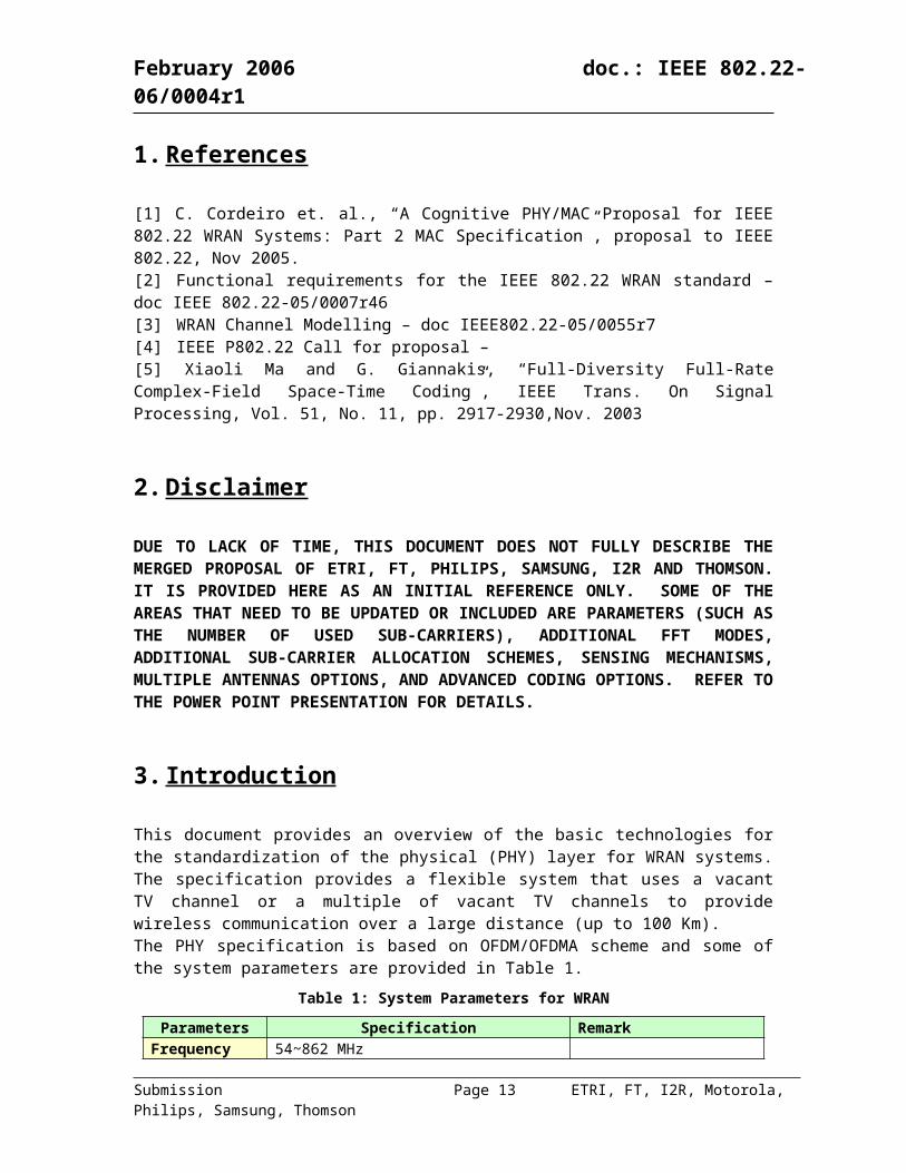
This document provides an overview of the basic technologies for the standardization of the physical (PHY) layer for WRAN systems. The specification provides a flexible system that uses a vacant TV channel or a multiple of vacant TV channels to provide wireless communication over a large distance (up to 100 Km).The PHY specification is based on OFDM/OFDMA scheme and some of the system parameters are provided in Table 1.
Table 1: System Parameters for WRAN
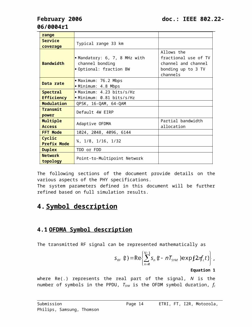
Parameters Specification RemarkFrequency range 54~862 MHzService coverage Typical range 33 km
Bandwidth Mandatory: 6, 7, 8 MHz with channel bonding Optional: fraction BW
Allows the fractional use of TV channel and channel bonding up to 3 TV channels
Data rate Maximum: 76.2 Mbps Minimum: 4.8 Mbps
Spectral Efficiency
Maximum: 4.23 bits/s/Hz Minimum: 0.81 bits/s/Hz
Modulation QPSK, 16-QAM, 64-QAMTransmit power Default 4W EIRPMultiple Access Adaptive OFDMA Partial bandwidth allocationFFT Mode 1024, 2048, 4096, 6144
Submission Page 10 ETRI, FT, I2R, Motorola, Philips, Samsung, Thomson
February 2006 doc.: IEEE 802.22-06/0004r1
Cyclic Prefix Mode ¼, 1/8, 1/16, 1/32
Duplex TDD or FDDNetwork topology Point-to-Multipoint Network
The following sections of the document provide details on the various aspects of the PHY specifications.The system parameters defined in this document will be further refined based on full simulation results.
4. Symbol description
4.1 OFDMA Symbol description
The transmitted RF signal can be represented mathematically as
, Equation 1
where Re(.) represents the real part of the signal, N is the number of symbols in the PPDU, TSYM is the OFDM symbol duration, fc is the carrier centre frequency and sn(t) is the complex base-band representation of the nth symbol.
The exact form of sn(t) is determined by the n and whether the symbol is part of the DS or US.
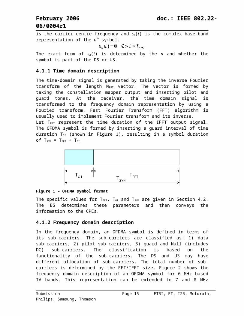
4.1.1 Time domain descriptionThe time-domain signal is generated by taking the inverse Fourier transform of the length N FFT
vector. The vector is formed by taking the constellation mapper output and inserting pilot and guard tones. At the receiver, the time domain signal is transformed to the frequency domain representation by using a Fourier transform. Fast Fourier Transform (FFT) algorithm is usually used to implement Fourier transform and its inverse.Let TFFT represent the time duration of the IFFT output signal. The OFDMA symbol is formed by inserting a guard interval of time duration TGI (shown in Figure 1), resulting in a symbol duration of TSYM = TFFT + TGI
Figure 1 – OFDMA symbol format
The specific values for TFFT, TGI and TSYM are given in Section 4.2. The BS determines these parameters and then conveys the information to the CPEs.
Submission Page 11 ETRI, FT, I2R, Motorola, Philips, Samsung, Thomson
February 2006 doc.: IEEE 802.22-06/0004r1
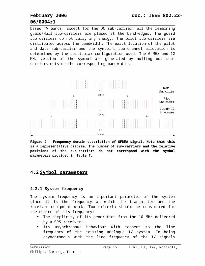
4.1.2 Frequency domain descriptionIn the frequency domain, an OFDMA symbol is defined in terms of its sub-carriers. The sub-carriers are classified as: 1) data sub-carriers, 2) pilot sub-carriers, 3) guard and Null (includes DC) sub-carriers. The classification is based on the functionality of the sub-carriers. The DS and US may have different allocation of sub-carriers. The total number of sub-carriers is determined by the FFT/IFFT size. Figure 2 shows the frequency domain description of an OFDMA symbol for 6 MHz based TV bands. This representation can be extended to 7 and 8 MHz based TV bands. Except for the DC sub-carrier, all the remaining guard/Null sub-carriers are placed at the band-edges. The guard sub-carriers do not carry any energy. The pilot sub-carriers are distributed across the bandwidth. The exact location of the pilot and data sub-carrier and the symbol’s sub-channel allocation is determined by the particular configuration used. The 6 MHz and 12 MHz version of the symbol are generated by nulling out sub-carriers outside the corresponding bandwidths.
Figure 2 – Frequency domain description of OFDMA signal. Note that this is a representative diagram. The number of sub-carriers and the relative positions of the sub-carriers do not correspond with the symbol parameters provided in Table 7.
4.2 Symbol parameters
4.2.1 System frequencyThe system frequency is an important parameter of the system since it is the frequency at which the transmitter and the receiver equipment work. Two criteria should be considered for the choice of this frequency:
The simplicity of its generation from the 10 MHz delivered by a GPS receiver; Its asynchronous behaviour with respect to the line frequency of the existing analogue
TV system. In being asynchronous with the line frequency of the TV signals (15.625 kHz in the case of PAL and SECAM) the system frequency reduces the level of interference of WRAN in an analogue TV co-channel.
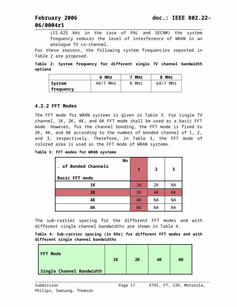
For these reasons, the following system frequencies reported in Table 2 are proposed.
Submission Page 12 ETRI, FT, I2R, Motorola, Philips, Samsung, Thomson
February 2006 doc.: IEEE 802.22-06/0004r1
Table 2: System frequency for different single TV channel bandwidth options
6 MHz 7 MHz 8 MHzSystem frequency 48/7 MHz 8 MHz 64/7 MHz
4.2.2 FFT ModesThe FFT mode for WRAN systems is given in Table 3. For single TV channel, 1K, 2K, 4K, and 6K FFT mode shall be used as a basic FFT mode. However, for the channel bonding, the FFT mode is fixed to 2K, 4K, and 6K according to the number of bonded channel of 1, 2, and 3, respectively. Therefore, in Table 3, the FFT mode of colored area is used as the FFT mode of WRAN systems.
Table 3: FFT modes for WRAN systems
No. of Bonded Channels
Basic FFT mode1 2 3
1K 1K 2K NA
2K 2K 4K 6K
4K 4K NA NA
6K 6K NA NA
The sub-carrier spacing for the different FFT modes and with different single channel bandwidths are shown in Table 4.
Table 4: Sub-carrier spacing (in KHz) for different FFT modes and with different single channel bandwidths
FFT Mode
Single Channel Bandwidth
1K 2K 4K 6K
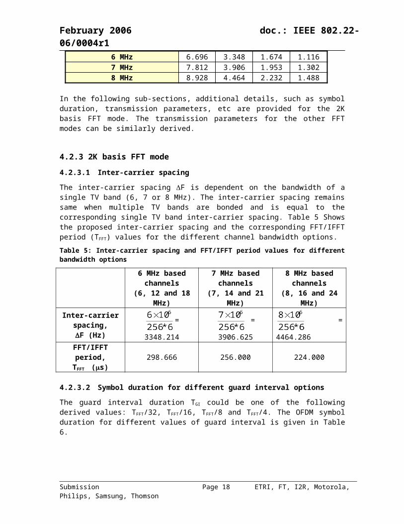
6 MHz 6.696 3.348 1.674 1.1167 MHz 7.812 3.906 1.953 1.3028 MHz 8.928 4.464 2.232 1.488
In the following sub-sections, additional details, such as symbol duration, transmission parameters, etc are provided for the 2K basis FFT mode. The transmission parameters for the other FFT modes can be similarly derived.
4.2.3 2K basis FFT mode4.2.3.1 Inter-carrier spacing
The inter-carrier spacing F is dependent on the bandwidth of a single TV band (6, 7 or 8 MHz). The inter-carrier spacing remains same when multiple TV bands are bonded and is equal to the corresponding single TV band inter-carrier spacing. Table 5 Shows the proposed inter-carrier spacing and the corresponding FFT/IFFT period (TFFT) values for the different channel bandwidth options.
Submission Page 13 ETRI, FT, I2R, Motorola, Philips, Samsung, Thomson
February 2006 doc.: IEEE 802.22-06/0004r1
Table 5: Inter-carrier spacing and FFT/IFFT period values for different bandwidth options
6 MHz based channels
(6, 12 and 18 MHz)
7 MHz based channels
(7, 14 and 21 MHz)
8 MHz based channels
(8, 16 and 24 MHz)Inter-carrier
spacing, F (Hz)
= 3348.214 = 3906.625 = 4464.286
FFT/IFFT period, TFFT (s) 298.666 256.000 224.000
4.2.3.2 Symbol duration for different guard interval options
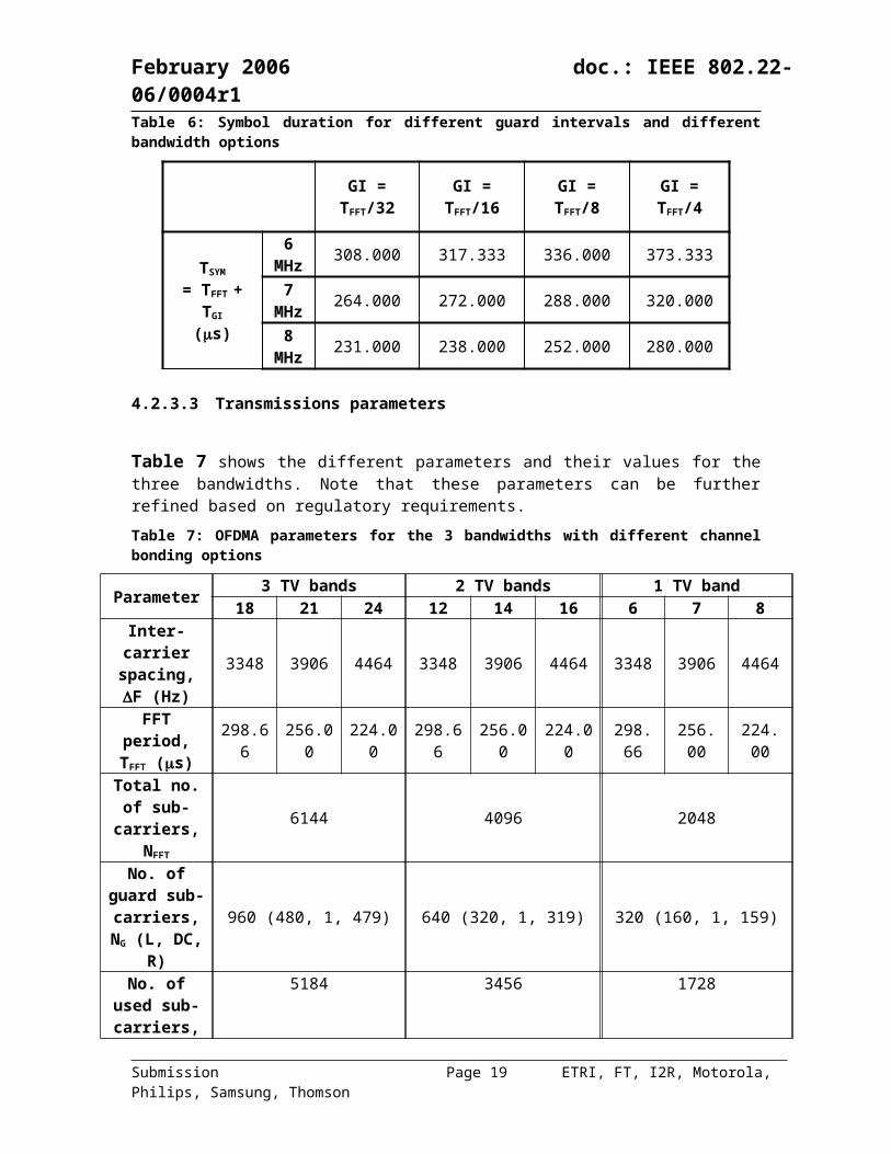
The guard interval duration TGI could be one of the following derived values: TFFT/32, TFFT/16, TFFT/8 and TFFT/4. The OFDM symbol duration for different values of guard interval is given in Table 6.
Table 6: Symbol duration for different guard intervals and different bandwidth options
GI = TFFT/32 GI = TFFT/16 GI = TFFT/8 GI = TFFT/4
TSYM = TFFT + TGI
(s)
6 MHz 308.000 317.333 336.000 373.333
7 MHz 264.000 272.000 288.000 320.000
8 MHz 231.000 238.000 252.000 280.000
4.2.3.3 Transmissions parameters
Table 7 shows the different parameters and their values for the three bandwidths. Note that these parameters can be further refined based on regulatory requirements.
Table 7: OFDMA parameters for the 3 bandwidths with different channel bonding options
Parameter 3 TV bands 2 TV bands 1 TV band18 21 24 12 14 16 6 7 8
Inter-carrier spacing, F (Hz)
3348 3906 4464 3348 3906 4464 3348 3906 4464
FFT period, TFFT (s) 298.66 256.00 224.00 298.66 256.00 224.00 298.66 256.00 224.00
Total no. of sub-carriers,
NFFT
6144 4096 2048
No. of guard sub-carriers, NG (L, DC, R)
960 (480, 1, 479) 640 (320, 1, 319) 320 (160, 1, 159)
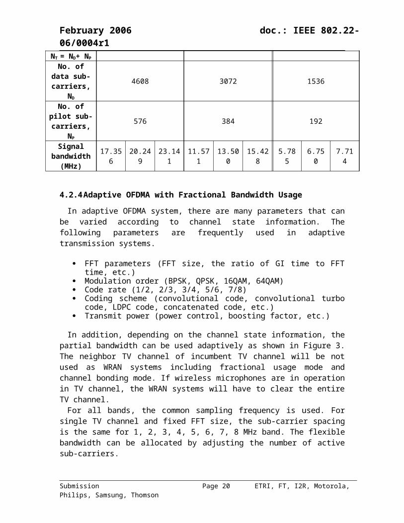
No. of used sub-carriers, NT = ND+ NP
5184 3456 1728
Submission Page 14 ETRI, FT, I2R, Motorola, Philips, Samsung, Thomson
February 2006 doc.: IEEE 802.22-06/0004r1
No. of data sub-carriers,
ND
4608 3072 1536
No. of pilot sub-carriers,
NP
576 384 192
Signal bandwidth
(MHz)
17.35620.249 23.141 11.571 13.500 15.428 5.785 6.750 7.714
4.2.4 Adaptive OFDMA with Fractional Bandwidth UsageIn adaptive OFDMA system, there are many parameters that can be varied according to
channel state information. The following parameters are frequently used in adaptive transmission systems.
FFT parameters (FFT size, the ratio of GI time to FFT time, etc.) Modulation order (BPSK, QPSK, 16QAM, 64QAM) Code rate (1/2, 2/3, 3/4, 5/6, 7/8) Coding scheme (convolutional code, convolutional turbo code, LDPC code,
concatenated code, etc.) Transmit power (power control, boosting factor, etc.)
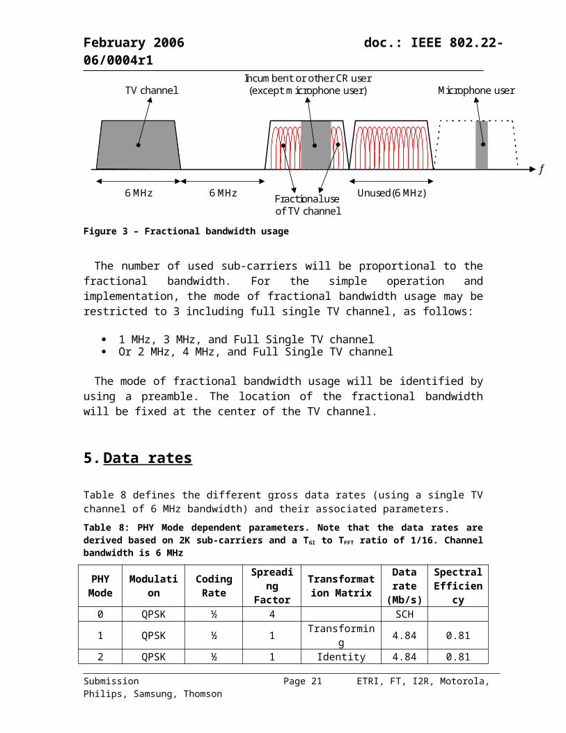
In addition, depending on the channel state information, the partial bandwidth can be used adaptively as shown in Figure 3. The neighbor TV channel of incumbent TV channel will be not used as WRAN systems including fractional usage mode and channel bonding mode. If wireless microphones are in operation in TV channel, the WRAN systems will have to clear the entire TV channel.
For all bands, the common sampling frequency is used. For single TV channel and fixed FFT size, the sub-carrier spacing is the same for 1, 2, 3, 4, 5, 6, 7, 8 MHz band. The flexible bandwidth can be allocated by adjusting the number of active sub-carriers.
6 MHz Unused(6 MHz)6 MHz
f
Incumbent or other CR user(except microphone user)TV channel Microphone user
Fractional useof TV channel
Figure 3 – Fractional bandwidth usage
Submission Page 15 ETRI, FT, I2R, Motorola, Philips, Samsung, Thomson
February 2006 doc.: IEEE 802.22-06/0004r1
The number of used sub-carriers will be proportional to the fractional bandwidth. For the simple operation and implementation, the mode of fractional bandwidth usage may be restricted to 3 including full single TV channel, as follows:
1 MHz, 3 MHz, and Full Single TV channel Or 2 MHz, 4 MHz, and Full Single TV channel
The mode of fractional bandwidth usage will be identified by using a preamble. The location of the fractional bandwidth will be fixed at the center of the TV channel.
5. Data rates
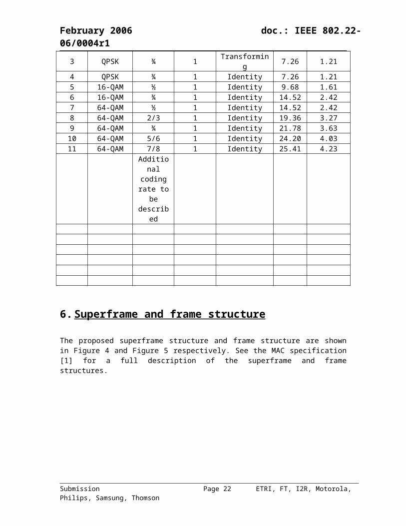
Table 8 defines the different gross data rates (using a single TV channel of 6 MHz bandwidth) and their associated parameters.
Table 8: PHY Mode dependent parameters. Note that the data rates are derived based on 2K sub-carriers and a TGI to TFFT ratio of 1/16. Channel bandwidth is 6 MHz
PHY Mode Modulation Coding
RateSpreading
FactorTransformation
Matrix
Data rate
(Mb/s)
Spectral Efficiency
0 QPSK ½ 4 SCH1 QPSK ½ 1 Transforming 4.84 0.812 QPSK ½ 1 Identity 4.84 0.813 QPSK ¾ 1 Transforming 7.26 1.214 QPSK ¾ 1 Identity 7.26 1.215 16-QAM ½ 1 Identity 9.68 1.616 16-QAM ¾ 1 Identity 14.52 2.427 64-QAM ½ 1 Identity 14.52 2.428 64-QAM 2/3 1 Identity 19.36 3.279 64-QAM ¾ 1 Identity 21.78 3.6310 64-QAM 5/6 1 Identity 24.20 4.0311 64-QAM 7/8 1 Identity 25.41 4.23
Additional coding rate
to be described
Submission Page 16 ETRI, FT, I2R, Motorola, Philips, Samsung, Thomson
February 2006 doc.: IEEE 802.22-06/0004r1
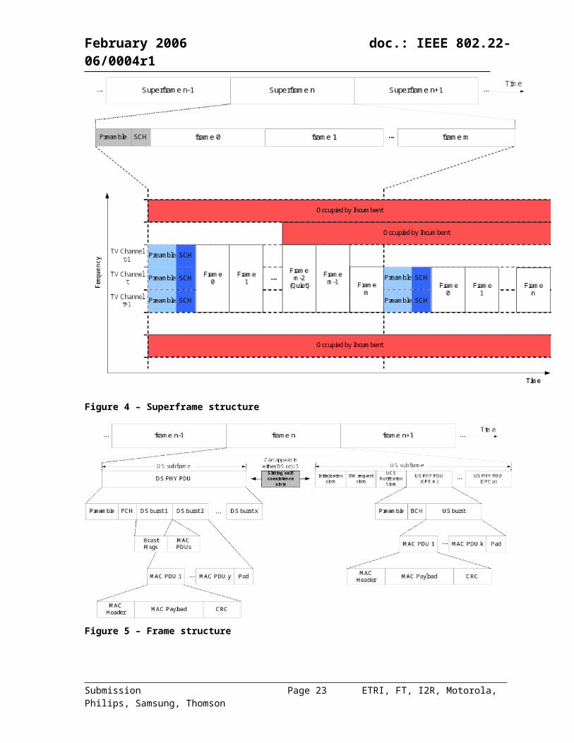
6. Superframe and frame structure
The proposed superframe structure and frame structure are shown in Figure 4 and Figure 5 respectively. See the MAC specification [1] for a full description of the superframe and frame structures.
Figure 4 – Superframe structure
Submission Page 17 ETRI, FT, I2R, Motorola, Philips, Samsung, Thomson
February 2006 doc.: IEEE 802.22-06/0004r1
Figure 5 – Frame structure
6.1 Preamble definition
The frequency domain sequences for the preambles are derived from the following length 5184 vector.
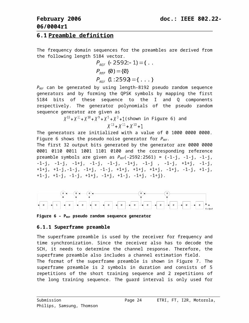
PREF can be generated by using length-8192 pseudo random sequence generators and by forming the QPSK symbols by mapping the first 5184 bits of these sequence to the I and Q components respectively. The generator polynomials of the pseudo random sequence generator are given as
(shown in Figure 6) and
The generators are initialized with a value of 0 1000 0000 0000. Figure 6 shows the pseudo noise generator for PREF.The first 32 output bits generated by the generator are 0000 0000 0001 0110 0011 1001 1101 0100 and the corresponding reference preamble symbols are given as PREF(-2592:2561) = {-1-j, -1-j, -1-j, -1-j, -1-j, -1+j, -1-j, -1-j, -1+j, -1-j , -1-j, +1+j, -1-j, +1+j, +1-j,-1-j, -1+j, -1-j, +1+j, +1+j, +1+j, -1+j, -1-j, +1-j, +1-j, +1-j, -1-j, +1+j, -1+j, +1-j, -1+j, -1+j}.
Figure 6 – PREF pseudo random sequence generator
Submission Page 18 ETRI, FT, I2R, Motorola, Philips, Samsung, Thomson
February 2006 doc.: IEEE 802.22-06/0004r1
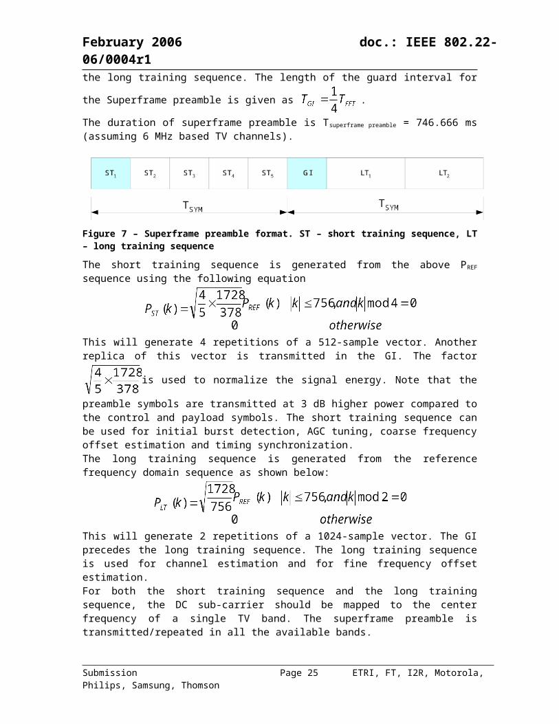
6.1.1 Superframe preambleThe superframe preamble is used by the receiver for frequency and time synchronization. Since the receiver also has to decode the SCH, it needs to determine the channel response. Therefore, the superframe preamble also includes a channel estimation field. The format of the superframe preamble is shown in Figure 7. The superframe preamble is 2 symbols in duration and consists of 5 repetitions of the short training sequence and 2 repetitions of the long training sequence. The guard interval is only used for the long training sequence. The
length of the guard interval for the Superframe preamble is given as .
The duration of superframe preamble is Tsuperframe preamble = 746.666 ms (assuming 6 MHz based TV channels).
Figure 7 – Superframe preamble format. ST – short training sequence, LT – long training sequence
The short training sequence is generated from the above PREF sequence using the following equation
This will generate 4 repetitions of a 512-sample vector. Another replica of this vector is
transmitted in the GI. The factor is used to normalize the signal energy. Note that the
preamble symbols are transmitted at 3 dB higher power compared to the control and payload symbols. The short training sequence can be used for initial burst detection, AGC tuning, coarse frequency offset estimation and timing synchronization.The long training sequence is generated from the reference frequency domain sequence as shown below:
This will generate 2 repetitions of a 1024-sample vector. The GI precedes the long training sequence. The long training sequence is used for channel estimation and for fine frequency offset estimation. For both the short training sequence and the long training sequence, the DC sub-carrier should be mapped to the center frequency of a single TV band. The superframe preamble is transmitted/repeated in all the available bands.
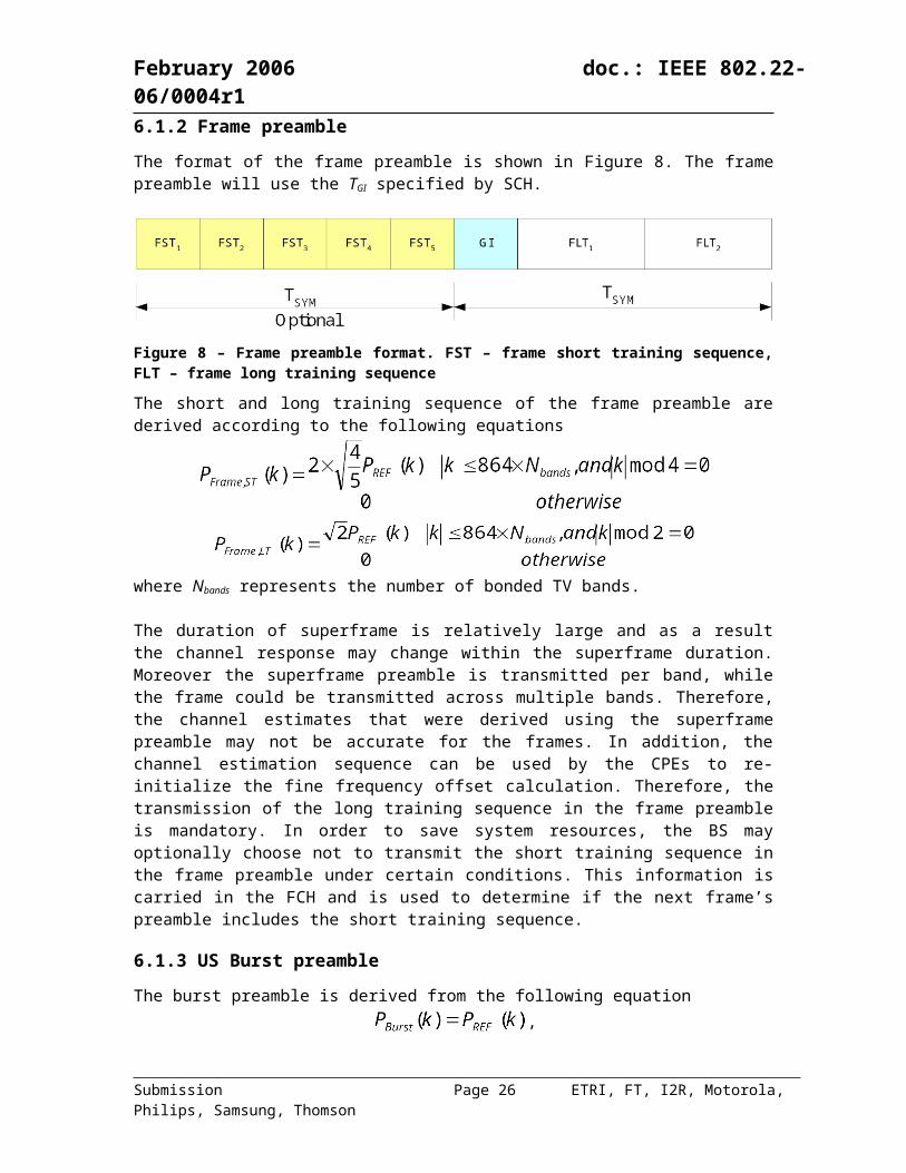
6.1.2 Frame preambleThe format of the frame preamble is shown in Figure 8. The frame preamble will use the TGI
specified by SCH.
Submission Page 19 ETRI, FT, I2R, Motorola, Philips, Samsung, Thomson
February 2006 doc.: IEEE 802.22-06/0004r1
Figure 8 – Frame preamble format. FST – frame short training sequence, FLT – frame long training sequence
The short and long training sequence of the frame preamble are derived according to the following equations
where Nbands represents the number of bonded TV bands.
The duration of superframe is relatively large and as a result the channel response may change within the superframe duration. Moreover the superframe preamble is transmitted per band, while the frame could be transmitted across multiple bands. Therefore, the channel estimates that were derived using the superframe preamble may not be accurate for the frames. In addition, the channel estimation sequence can be used by the CPEs to re-initialize the fine frequency offset calculation. Therefore, the transmission of the long training sequence in the frame preamble is mandatory. In order to save system resources, the BS may optionally choose not to transmit the short training sequence in the frame preamble under certain conditions. This information is carried in the FCH and is used to determine if the next frame’s preamble includes the short training sequence.
6.1.3 US Burst preamble The burst preamble is derived from the following equation
,where k represents the sub-carrier indices in the CPE’s allocated sub-channels. The burst preamble is transmitted in the first symbol of the burst transmission.The burst preamble is used by the BS to estimate the channel from the CPE to the BS. Transmission of the burst preamble on each burst is not very efficient under certain channel conditions. Therefore, the burst preamble field is made optional. The US-MAP field contains the information on burst preamble. The CPEs will only use their allocated sub-channels to transmit the burst preamble.
6.1.4 CBP preambleThe structure of the CBP preamble is similar to that of the Superframe preamble. The CBP preamble is generated similar to the one for the Superframe preamble except that the last instead of the first 5184 samples from the 8191-length sequence are used to generate the I and Q components of the reference symbol sequence.
Submission Page 20 ETRI, FT, I2R, Motorola, Philips, Samsung, Thomson
February 2006 doc.: IEEE 802.22-06/0004r1
6.2 Control header and map definition s
6.2.1 Superframe control header (SCH)The super frame control header includes information such as the number of channels, number of frames, channel number, etc. It also includes a variable number of IEs, due to which the length of SCH is also variable (with a minimum of 19 bytes and a maximum of 42 bytes). Additional details on the SCH are provided in the MAC specification.The superframe control header is encoded using the methods/modules described in Section 8. The SCH is transmitted using the basic data rate mode. The 15-bit randomizer initialisation sequence shall be set to all 1s (i.e. 1111 1111 1111 111). The SCH shall be decoded by all the CPEs associated with that BS (or in the region of that BS). The super frame control header is transmitted in all the sub-channels. Since the superframe control header has to be decoded by all the CPEs in the range of the BS, the SCH has to be repeated in all the bands.The 42 bytes of the SCH are encoded by a rate-1/2 convolutional coder and after interleaving are mapped using QPSK constellation resulting in 336 symbols. In order to improve the robustness of SCH and to make better utilization of the available sub-carriers, spreading by a factor of 4 is applied to the output of the mapper. This will result in 1344 symbols occupying 28 sub-channels (see Section 7.1 for the definition of sub-channel). This will free up 2 sub-channels on each of the band-edges, which are therefore defined as guard sub-channels. The additional guard sub-carriers at the band-edges will enable the CPEs to better decode the SCH. The 2K IFFT vector thus formed is replicated to generate the 4K and 6K length IFFT vectors. The TGI to TFFT ratio is ¼ for the SCH.
6.2.1.1 Sub-carrier allocation for SCH
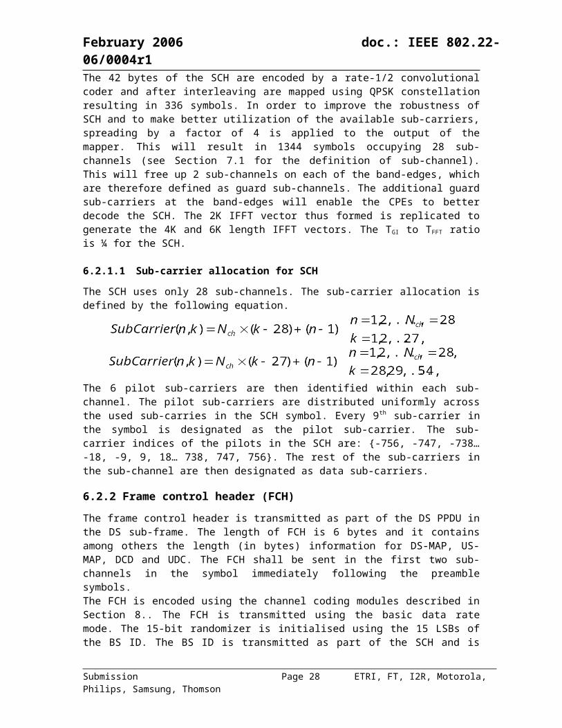
The SCH uses only 28 sub-channels. The sub-carrier allocation is defined by the following equation.
The 6 pilot sub-carriers are then identified within each sub-channel. The pilot sub-carriers are distributed uniformly across the used sub-carries in the SCH symbol. Every 9 th sub-carrier in the symbol is designated as the pilot sub-carrier. The sub-carrier indices of the pilots in the SCH are: {-756, -747, -738… -18, -9, 9, 18… 738, 747, 756}. The rest of the sub-carriers in the sub-channel are then designated as data sub-carriers.
6.2.2 Frame control header (FCH)The frame control header is transmitted as part of the DS PPDU in the DS sub-frame. The length of FCH is 6 bytes and it contains among others the length (in bytes) information for DS-MAP, US-MAP, DCD and UDC. The FCH shall be sent in the first two sub-channels in the symbol immediately following the preamble symbols.The FCH is encoded using the channel coding modules described in Section 8. The FCH is transmitted using the basic data rate mode. The 15-bit randomizer is initialised using the 15 LSBs of the BS ID. The BS ID is transmitted as part of the SCH and is available to the CPEs. The 48 FCH bits are encoded and mapped onto 48 data sub-carriers in sub-channel #1 (Note that the sub-carrier allocation for FCH is as defined in Section 7.1). In order to increase the robustness of the
Submission Page 21 ETRI, FT, I2R, Motorola, Philips, Samsung, Thomson
February 2006 doc.: IEEE 802.22-06/0004r1
FCH, the encoded and mapped FCH data is re-transmitted in sub-channel #2. If SFCH,1(k) represents the symbol transmitted on sub-carrier k in sub-channel 1, then the symbol transmitted on sub-channel k in sub-channel 2, SFCH,2(k) is given as
The receiver should combine corresponding symbols form the two sub-channels and decode the FCH data to determine the lengths of the following fields in the frames.
6.2.3 US Burst control header (BCH)The burst control header is sent as part of the US PPDUs in the US sub-frame. Each CPE will use it allocated sub-channels to send the BCH in the symbol immediately following the US preamble symbols. If US preamble is not transmitted, then the BCH symbol shall be the first symbol of the US PPDUs. The BCH contains the BS ID and CPE ID information.The BCH is encoded using the channel coding modules described in Section 8. The BCH is transmitted at the same data rate as the rest of the payload symbols. The randomizer is initialized using the 8 LSBs of the BS ID and 7 LSBs of CPE ID as shown in Figure 9.
Figure 9 – Scrambler initialization vector for BCH
6.2.4 Downstream MAP (DS-MAP), Upstream MAP (US-MAP), Downstream Channel Descriptor (DCD) and Upstream Channel Descriptor (UCD)
The lengths of DS-MAP, US-MAP, DCD and UCD fields are variable and are defined in FCH. These fields are transmitted using the base data rate mode. The DS-MAP is transmitted in the logical channels numbers immediately following the FCH logical channel numbers. The DS-MAP is followed by the US-MAP, DCD and UCD in that order. The number of sub-channels required to transmit these fields is determined by their lengths and could possibly exceed the number of sub-channels allocated per symbol. In that scenario, the transmission of these fields will continue in the next symbol starting with the first logical sub-channel. It is anticipated that no more than 2 symbols would be required to transmit the FCH, MAP and descriptor information. The unused sub-channels in the second symbol can be used for DS transmissions.
7. OFDMA sub-carrier allocation
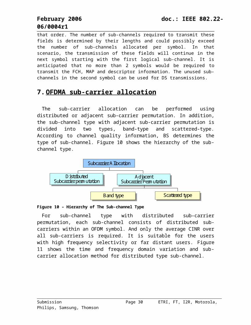
The sub-carrier allocation can be performed using distributed or adjacent sub-carrier permutation. In addition, the sub-channel type with adjacent sub-carrier permutation is divided into two types, band-type and scattered-type. According to channel quality information, BS determines the type of sub-channel. Figure 10 shows the hierarchy of the sub-channel type.
Submission Page 22 ETRI, FT, I2R, Motorola, Philips, Samsung, Thomson
February 2006 doc.: IEEE 802.22-06/0004r1
Subcarrier Allocation
AdjacentSubcarrier Permutation
AdjacentSubcarrier Permutation
DistributedSubcarrier permutation
DistributedSubcarrier permutation
Scattered typeScattered typeBand typeBand type
Figure 10 – Hierarchy of The Sub-channel Type
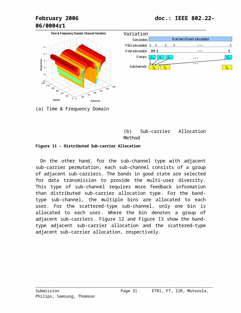
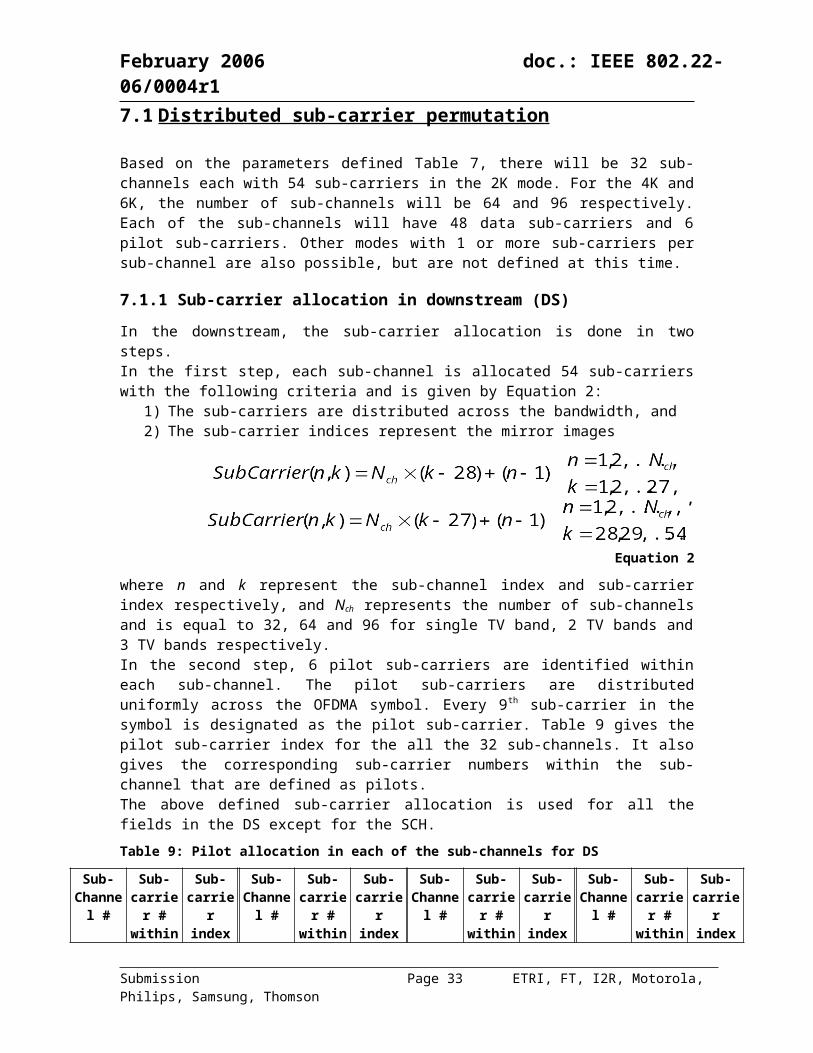
For sub-channel type with distributed sub-carrier permutation, each sub-channel consists of distributed sub-carriers within an OFDM symbol. And only the average CINR over all sub-carriers is required. It is suitable for the users with high frequency selectivity or far distant users. Figure 11 shows the time and frequency domain variation and sub-carrier allocation method for distributed type sub-channel.
(a) Time & Frequency Domain Variation
Groups
Number of used subcarriersSubcarriers
G0
Pilot subcarriers
Data subcarriers
. . .
. . .S0
. . .
. . .
G1 G2 GN
S1 SMSubchannels
(b) Sub-carrier Allocation Method
Figure 11 – Distributed Sub-carrier Allocation
On the other hand, for the sub-channel type with adjacent sub-carrier permutation, each sub-channel consists of a group of adjacent sub-carriers. The bands in good state are selected for data transmission to provide the multi-user diversity. This type of sub-channel requires more feedback information than distributed sub-carrier allocation type. For the band-type sub-channel, the multiple bins are allocated to each user. For the scattered-type sub-channel, only one bin is allocated to each user. Where the bin denotes a group of adjacent sub-carriers.
Submission Page 23 ETRI, FT, I2R, Motorola, Philips, Samsung, Thomson
February 2006 doc.: IEEE 802.22-06/0004r1
Figure 12 and Figure 13 show the band-type adjacent sub-carrier allocation and the scattered-type adjacent sub-carrier allocation, respectively.
(a) Time & Frequency Domain Variation
SymbolSymbol
User 0
User 1
User 2
Band #1Band #1
…
BINBIN
Band #2Band #2
Band #3Band #3
Band #24Band #24
…
(b) Subcarrier Allocation MethodFigure 12 – Band-Type Adjacent Sub-carrier Allocation
Submission Page 24 ETRI, FT, I2R, Motorola, Philips, Samsung, Thomson
February 2006 doc.: IEEE 802.22-06/0004r1
(a) Time & Frequency Domain Variation
Band #5Band #5
Band #4Band #4
SymbolSymbol
User 0
User 1
User 2
BINBINBand #1Band #1
…
Band #2Band #2
Band #3Band #3
Band #48Band #48
…
User 3
(b) Subcarrier Allocation Method
Submission Page 25 ETRI, FT, I2R, Motorola, Philips, Samsung, Thomson
February 2006 doc.: IEEE 802.22-06/0004r1
Figure 13 – Scattered-Type Adjacent Sub-carrier Allocation
In the proposal, the sub-channel type of distributed, scattered-type adjacent, and band-type adjacent are used in the best, medium, and worse channel environment, respectively.
7.1 Distributed sub-carrier permutation
Based on the parameters defined Table 7, there will be 32 sub-channels each with 54 sub-carriers in the 2K mode. For the 4K and 6K, the number of sub-channels will be 64 and 96 respectively. Each of the sub-channels will have 48 data sub-carriers and 6 pilot sub-carriers. Other modes with 1 or more sub-carriers per sub-channel are also possible, but are not defined at this time.
7.1.1 Sub-carrier allocation in downstream (DS)In the downstream, the sub-carrier allocation is done in two steps. In the first step, each sub-channel is allocated 54 sub-carriers with the following criteria and is given by Equation 2:
1) The sub-carriers are distributed across the bandwidth, and2) The sub-carrier indices represent the mirror images
, Equation 2
where n and k represent the sub-channel index and sub-carrier index respectively, and Nch
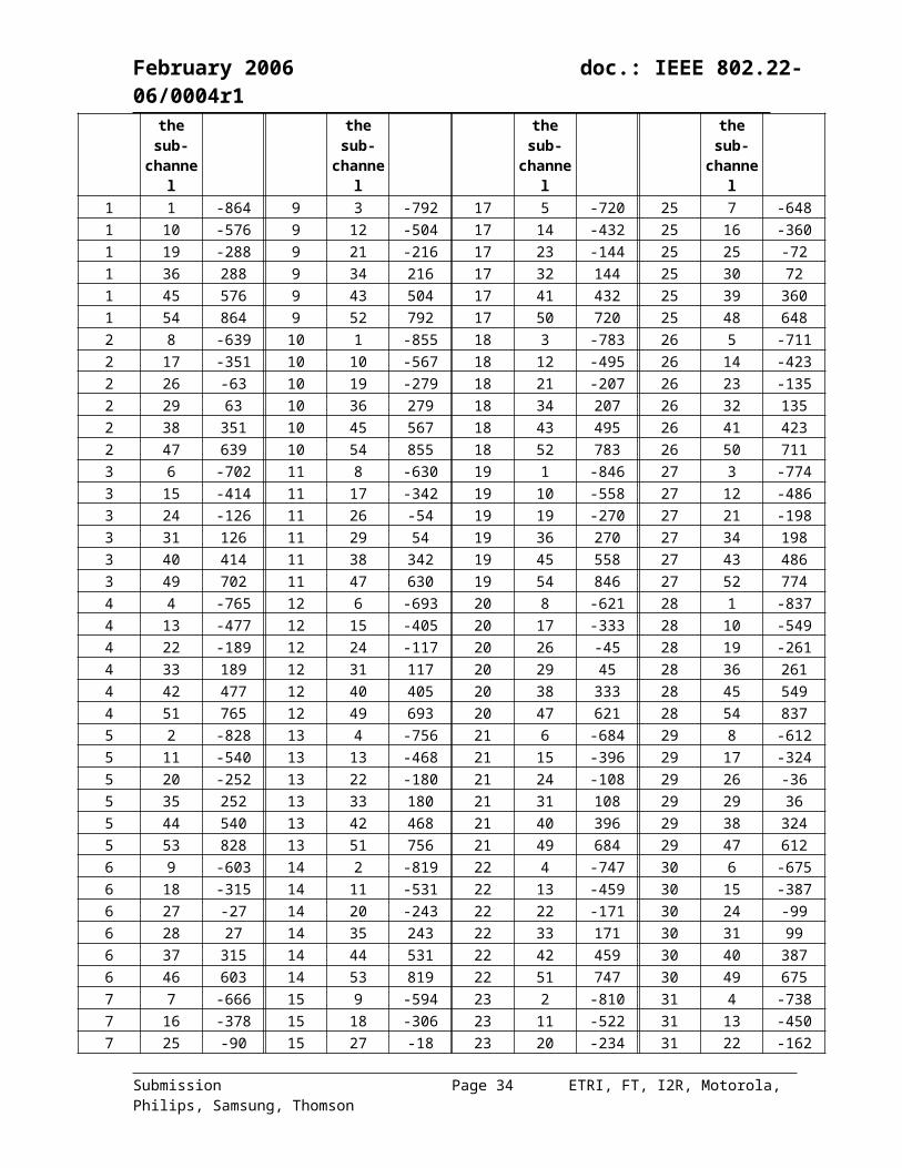
represents the number of sub-channels and is equal to 32, 64 and 96 for single TV band, 2 TV bands and 3 TV bands respectively.In the second step, 6 pilot sub-carriers are identified within each sub-channel. The pilot sub-carriers are distributed uniformly across the OFDMA symbol. Every 9 th sub-carrier in the symbol is designated as the pilot sub-carrier. Table 9 gives the pilot sub-carrier index for the all the 32 sub-channels. It also gives the corresponding sub-carrier numbers within the sub-channel that are defined as pilots. The above defined sub-carrier allocation is used for all the fields in the DS except for the SCH.
Table 9: Pilot allocation in each of the sub-channels for DS
Sub-Channel
#
Sub-carrier # within
the sub-channel
Sub-carrier index
Sub-Channel
#
Sub-carrier # within
the sub-channel
Sub-carrier index
Sub-Channel
#
Sub-carrier # within
the sub-channel
Sub-carrier index
Sub-Channel
#
Sub-carrier # within
the sub-channel
Sub-carrier index
1 1 -864 9 3 -792 17 5 -720 25 7 -6481 10 -576 9 12 -504 17 14 -432 25 16 -3601 19 -288 9 21 -216 17 23 -144 25 25 -721 36 288 9 34 216 17 32 144 25 30 721 45 576 9 43 504 17 41 432 25 39 3601 54 864 9 52 792 17 50 720 25 48 6482 8 -639 10 1 -855 18 3 -783 26 5 -711
Submission Page 26 ETRI, FT, I2R, Motorola, Philips, Samsung, Thomson
February 2006 doc.: IEEE 802.22-06/0004r1
2 17 -351 10 10 -567 18 12 -495 26 14 -4232 26 -63 10 19 -279 18 21 -207 26 23 -1352 29 63 10 36 279 18 34 207 26 32 1352 38 351 10 45 567 18 43 495 26 41 4232 47 639 10 54 855 18 52 783 26 50 7113 6 -702 11 8 -630 19 1 -846 27 3 -7743 15 -414 11 17 -342 19 10 -558 27 12 -4863 24 -126 11 26 -54 19 19 -270 27 21 -1983 31 126 11 29 54 19 36 270 27 34 1983 40 414 11 38 342 19 45 558 27 43 4863 49 702 11 47 630 19 54 846 27 52 7744 4 -765 12 6 -693 20 8 -621 28 1 -8374 13 -477 12 15 -405 20 17 -333 28 10 -5494 22 -189 12 24 -117 20 26 -45 28 19 -2614 33 189 12 31 117 20 29 45 28 36 2614 42 477 12 40 405 20 38 333 28 45 5494 51 765 12 49 693 20 47 621 28 54 8375 2 -828 13 4 -756 21 6 -684 29 8 -6125 11 -540 13 13 -468 21 15 -396 29 17 -3245 20 -252 13 22 -180 21 24 -108 29 26 -365 35 252 13 33 180 21 31 108 29 29 365 44 540 13 42 468 21 40 396 29 38 3245 53 828 13 51 756 21 49 684 29 47 6126 9 -603 14 2 -819 22 4 -747 30 6 -6756 18 -315 14 11 -531 22 13 -459 30 15 -3876 27 -27 14 20 -243 22 22 -171 30 24 -996 28 27 14 35 243 22 33 171 30 31 996 37 315 14 44 531 22 42 459 30 40 3876 46 603 14 53 819 22 51 747 30 49 6757 7 -666 15 9 -594 23 2 -810 31 4 -7387 16 -378 15 18 -306 23 11 -522 31 13 -4507 25 -90 15 27 -18 23 20 -234 31 22 -1627 30 90 15 28 18 23 35 234 31 33 1627 39 378 15 37 306 23 44 522 31 42 4507 48 666 15 46 594 23 53 810 31 51 7388 5 -729 16 7 -657 24 9 -585 32 2 -8018 14 -441 16 16 -369 24 18 -297 32 11 -5138 23 -153 16 25 -81 24 27 -9 32 20 -2258 32 153 16 30 81 24 28 9 32 35 2258 41 441 16 39 369 24 37 297 32 44 5138 50 729 16 48 657 24 46 585 32 53 801
7.1.2 Sub-carrier allocation in Upstream (US)The 2-step sub-carrier allocation is also used for the US. In the first step, Equation 2 is used to allocate 54 sub-carriers in each of the 32 sub-channels. In the second step, 6 pilot sub-carriers are identified within each sub-channel.The following equation defines the location of pilot sub-carriers within the given sub-channel’s 54 sub-carriers:
Submission Page 27 ETRI, FT, I2R, Motorola, Philips, Samsung, Thomson
February 2006 doc.: IEEE 802.22-06/0004r1
, Equation 3
where is the pilot number in sub-channel n.Optionally, the pilot sub-carriers in Upstream transmission can be transmitted at a higher power (about 3 dB) compared to the data sub-carriers. The remaining indices are designated as data sub-carriers.
7.2 Additional pilot pattern s
Generally speaking, the block-type pilot pattern is suitable for frequency-selective fading channel, and the comb-type pilot pattern is suitable for fast time-selective fading channel. However, the number of used pilots is a trade-off between throughput and channel estimation performance. A combination pilot pattern of comb- and block-type is proposed in this section. To determine the sub-optimal period between pilots in the sub-carrier and symbol direction, we need to consider the Doppler spread and the maximum delay spread of the wireless channel. As the WRAN channel has the characteristics of the frequency-selective but slow fading, the pilot symbol spacing is sparse but the pilot sub-carrier spacing is dense.
Figure 14 shows an example of the proposed pilot pattern. The pilot symbol period and pilot sub-carrier period are varied with channel state information. The pilots are placed at specified intervals in the OFDM frequency-time signal space, so that the frequency and time interpolation of the channel is used for the channel estimation.
Pilot Symbol Period(variable)
Pilot
Subc
arrie
r Per
iod(v
ariab
le)
OFDMA Symbol Direction
Subc
arrie
r Dire
ctio
n
DataBoosted Pilot
Figure 14 – Additional pilot patterns
8. Channel coding
Channel coding includes data scrambling, convolutional coding/duo-binary convolutional turbo coding, puncturing, bit interleaving and constellation mapping. Figure 15 shows the mandatory channel coding process. The channel coder processes the control headers and the PSDU portion of the PPDU. The channel coder shall not process the preamble part of the PPDU.
Submission Page 28 ETRI, FT, I2R, Motorola, Philips, Samsung, Thomson
February 2006 doc.: IEEE 802.22-06/0004r1
For the purpose of channel coding, each data burst is further sub-divided in to data blocks as shown in Figure 16. Each block of encoded data will be mapped and transmitted on a sub-channel. It is assumed here that distributed sub-carrier allocation is used to define sub-channels. If contiguous sub-carrier allocation is used then multiple blocks of encoded data will be mapped and transmitted on multiple sub-channels (not defined in this section).
Figure 15 – Channel coding process
Figure 16 – Partitioning of a data burst into data blocks
8.1 Data scrambling
The PSDU data is first processed by the data scrambler using a pseudo random binary sequence (PRBS) generator. The PRBS generator polynomial is and is shown in Figure 17. The preamble and the control header fields of the PPDU are not scrambled. The data scrambler is initialised on each burst and the 15-bit initialisation vector is created as shown in Figure 18. The generation of the initialization vector for control headers is described in Section 6.2. The pad bits if present shall be scrambled.
Figure 17 – Pseudo random binary sequence generator for data scrambler
Submission Page 29 ETRI, FT, I2R, Motorola, Philips, Samsung, Thomson
February 2006 doc.: IEEE 802.22-06/0004r1
Figure 18 – Data scrambler initialization vector for the data bursts
8.2 Forward Error Correction (FEC)
Convolutional code is mandatory and there are two proposed optional modes.
8.2.1 Convolutional code (CC) mode (mandatory)8.2.1.1 Convolutional coding
The data burst is encoded using a rate – ½ binary convolutional encoder. The constraint length of this coder is equal to 7 and its generator polynomials are 171o and 133o. Figure 19 shows the pictorial depiction of the generator polynomials. Output A and output B represent the first and second output bits respectively of this encoder. The convolutional coder shall be initialised at the beginning of the control headers and at the beginning of the each burst. Tail biting shall be used with control headers, while tail bits (6 in number) should be used with the burst or PSDU data. This implies that for the case of control headers, the encoder memory is initialised with the last 6 bits in the header; and for the case of PSDU data, the encoder memory is initialised to all zero state.
Figure 19 – Rate – ½ convolutional coder with generator polynomials 171o, 133o. The delay element represents a delay of 1 bit
8.2.1.2 Puncturing
Different coding rates can be obtained by puncturing the output of the convolutional coder. Table10 shows the different rates that can be derived from the output of rate – ½ convolutional coder and the associated puncturing patterns.Decoding by using Viterbi algorithm is recommended. At the receiver, zeros are inserted in the locations of the punctured bits before the Viterbi decoder.
Submission Page 30 ETRI, FT, I2R, Motorola, Philips, Samsung, Thomson
February 2006 doc.: IEEE 802.22-06/0004r1
Table 10: Puncturing and bit-insertion for the different coding rates
Code rate ½ 2/3 ¾ 5/6Convolutional coder output A1B1 A1B1A2B2 A1B1A2B2A3B3 A1B1A2B2A3B3A4B4A5B5
Puncturer output/bit-
inserter inputA1B1 A1B1B2 A1B1B2A3 A1B1B2A3B4A5
Decoder input A1B1 A1B10B2 A1B10B2A30 A1B10B2A300B4A50
8.2.2 Duo-binary convolutional Turbo code (CTC) mode (optional)8.2.2.1 Duo-binary convolutional turbo coding
The duo-Binary Turbo Codes use Circular Recursive Systematic Convolutional (CRSC) Codes as component codes, with double-binary input.The encoding system is fed by blocks of k bits or N couples (k=2xN). N is a multiple of 4 (k is a multiple of 8) and should be comprised between 32 and 4096. It is illustrated in Figure 20.
Figure 20 – Duo-binary convolutional turbo code: Encoding scheme
The polynomials, which shall be used for the connections, are described in octal and symbolic notations as follows:
- for the feedback branch: 15 (in octal), equivalently 1+D+D3 (in symbolic notation);
- for the Y1 and Y2 parity bits, 13, equivalently 1+D2+D3;
The input A shall be connected to tap “1” of the shift register and the input “B” shall be connected to the input taps “1”, D and D2.
Submission Page 31 ETRI, FT, I2R, Motorola, Philips, Samsung, Thomson

February 2006 doc.: IEEE 802.22-06/0004r1
This first encoding is called C1 encoding. After initialisation by the circulation state , the encoder shall be fed by the sequence in the natural order with incremental address i = 0,…,N-1. This second encoding is called C2 encoding. After initialisation by the circulation state
, the encoder shall be fed by the interleaved sequence with incremental address j = 0,… N-1. The function (j) that gives the natural address i of the considered couple, when reading it at place j for the second encoding, is given in 8.2.2.2.
8.2.2.2 CTC interleaver
In the CTC interleaver, the permutation shall be done on two levels:- the first one inside the couples (level 1),- the second one between couples (level 2),
The permutation is described in the following algorithm. Set the permutation parameters P0, P1, P2 and P3.
These parameters depend on the size of the sequence to be encoded. For example, for MPEG2-TS packet size (188 bytes): P0 = 19, P1 = 376, P2 = 224 and P3 = 600.
j = 0,… N-1. level 1
if j mod. 2 = 0, let (A,B) = (B,A) (invert the couple) level 2
- if j mod. 4 = 0, then P = 0;- if j mod. 4 = 1, then P = N/2 + P1;- if j mod. 4 = 2, then P = P2;- if j mod. 4 = 3, then P = N/2 + P3.
i = P0*j + P + 1 mod. N
8.2.2.3 Determination of the circulation states
The state of the encoder is denoted S (0 S 7) with S = 4.s1 + 2.s2 + s3 (see Table 2). The circulation states and shall be determined by the following operations:
1. Initialise the encoder with state 0. Encode the sequence in the natural order for the determination of or in the interleaved order for the determination of (without producing redundancy). In both cases, the final state of the encoder is denoted .
2. According to the length N of the sequence, the following correspondence shall be used to find and (see the following table).
Table 11: Circulation state correspondence table
Nmod.70 1 2 3 4 5 6 7
1 Sc=0 Sc=6 Sc=4 Sc=2 Sc=7 Sc=1 Sc=3 Sc=52 Sc=0 Sc=3 Sc=7 Sc=4 Sc=5 Sc=6 Sc=2 Sc=1
Submission Page 32 ETRI, FT, I2R, Motorola, Philips, Samsung, Thomson
February 2006 doc.: IEEE 802.22-06/0004r1
3 Sc=0 Sc=5 Sc=3 Sc=6 Sc=2 Sc=7 Sc=1 Sc=44 Sc=0 Sc=4 Sc=1 Sc=5 Sc=6 Sc=2 Sc=7 Sc=35 Sc=0 Sc=2 Sc=5 Sc=7 Sc=1 Sc=3 Sc=4 Sc=66 Sc=0 Sc=7 Sc=6 Sc=1 Sc=3 Sc=4 Sc=5 Sc=2
8.2.2.4 Code rate and puncturing
Three code rates are defined here (more code rates can be defined if required): R = ½, 2/3, and ¾. These rates shall be achieved through selectively deleting the parity bits (puncturing). The puncturing pattern defined in the following table shall be applied.
Table 12: Puncturing patterns for turbo codes (“1”=keep, “0”=delete)
Code Rate Puncturing vector1/2 Y = [1 1 1 1 1 1]2/3 Y = [1 0 1 0 1 0]3/4 Y = [1 0 0 1 0 0]
8.2.3 Low density parity check codes (LDPC) mode (Optional)8.2.3.1 802.16 LDPC code
8.2.3.2 ETRI LDPC code
Please refer to the presentation [doc #] for additional details on the LDPC codes.
8.2.4 Shortened block turbo codes (SBTC) mode (Optional)The BTC is constructed by the product of two simple component codes, which are binary extended Hamming codes with a special design or parity check codes. Table 13 specifies the parity check matrix for the Hamming codes. Actually, all the columns of the parity check matrix for n = 15 are the binary representation of integers 1 to 15 (the topmost part corresponds to the least-significant bit in the binary representation of an integer). Similarly, all the columns of the parity check matrix for n = 31 and 63 are the binary representation of integers 1 to 31 and integers 1 to 63, respectively. Note that with this encoding scheme, the parity check bits are no longer located together at the end of the code word. In general, for a (2m-1,2m-1-m) Hamming code, the parity-check positions are located in columns numbered 1, 2, 4, …, 2m-1 of the parity check matrix. To create extended Hamming codes, the overall even parity check bit is added at the end of each code word.
Table 13: Parity check matrix for the Hamming codes in OFDMA
n’ K’ Parity check matrix
15 11
154111000111000110110101101
Submission Page 33 ETRI, FT, I2R, Motorola, Philips, Samsung, Thomson
February 2006 doc.: IEEE 802.22-06/0004r1
31 26
315111000111000111000110110101101
63 57
636111000111000111000111000110110101101
With the aid of Figure 21, the procedure to construct product code is listed as follows:1) Place (ky kx) information bits in information area (the blank area in Figure 21). The
information bits may be placed in columns with indexes from 1 to nx-1, except for columns 2i
with i = 0, 1, 2, …, nx-kx-2 (nx-kx-1 parity check bits). Similarly, information bits may be located in rows with indexes 1 to ny except for rows with indexes 2j with j = 0, 1, 2, …, ny-ky-2 (ny-ky-1 parity check bits).
2) Compute the parity check bits of ky rows using the corresponding parity check matrix in Table 13 and inserting them in the corresponding positions signed by ;
3) Compute the parity check bits of kx columns using the corresponding parity check matrix in Table 13 and inserting them in the corresponding positions signed by and ;
4) Calculate and append the extended parity check bits to the corresponding rows and columns.5) The overall block size of such a product code is n = nx × ny, the total number of information
bits k = kx × ky, and the code rate is R = Rx × Ry,, where Ri = ki/ni, i = x, y. The Hamming distance of the product code is d = dx × dy,. Data bit ordering for the composite BTC block is the first bit in the first row is the LSB and the last data bit in the last data row is the MSB.
Transmission of the block over the channel shall occur in a linear fashion, with all bits of the first row transmitted left to right followed by the second row, etc.To match a required packet size, BTCs may be shortened by removing symbols from the BTC array. In the two-dimensional case, rows, columns, or parts thereof can be removed until the appropriate size is reached. There are three steps in the process of shortening product codes:
o Step 1) Remove Ix rows and Iy columns from the two-dimensional code. This is equivalent to shortening the constituent codes that make up the product code.
o Step 2) Remove D individual bits from the first row of the two-dimensional code starting with the LSB.
o Step 3) Use if the product code specified from Step 1) and Step 2) of this sub-clause has a non-integer number of data bytes. In this case, the Q right LSBs are zero-filled by the encoder. After decoding at the receive end, the decoder shall strip off these unused bits and only the specified data payload is passed to the next higher level in the PHY. The same general method is used for shortening the last code word in a message where the available data bytes do not fill the available data bytes in a code block.
Submission Page 34 ETRI, FT, I2R, Motorola, Philips, Samsung, Thomson

February 2006 doc.: IEEE 802.22-06/0004r1
These three processes of code shortening are depicted in Figure 22. The new coded block length of the code is (nx – Ix)(ny – Iy) – D. The corresponding information length is given as (kx – Ix)(ky – Iy) – D – Q. Consequently, the code rate is given by the following equation:
Figure 21 – Block turbo code (BTC) structure
Submission Page 35 ETRI, FT, I2R, Motorola, Philips, Samsung, Thomson
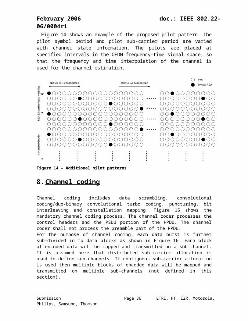
February 2006 doc.: IEEE 802.22-06/0004r1
Figure 22 – Shortened BTC (SBTC) structure
The basic sizes of the useful data payloads for different modulation type and encoding rate are displayed in Table 14. Table 15 gives the block sizes for the optional modulation and coding schemes using BTC. Table 16 gives the code parameters for each of the possible data and coded block size.
Table 14: Data payload for a sub-channel
Modulation QPSK 8PSK 16 QAM 64 QAM Coded Bytes
Encoding rate 1/2 3/4 1/2 2/3 1/2 3/4 1/2 2/3 3/4
Data payload
6 9 12
12 18 12 18 24
Submission Page 36 ETRI, FT, I2R, Motorola, Philips, Samsung, Thomson
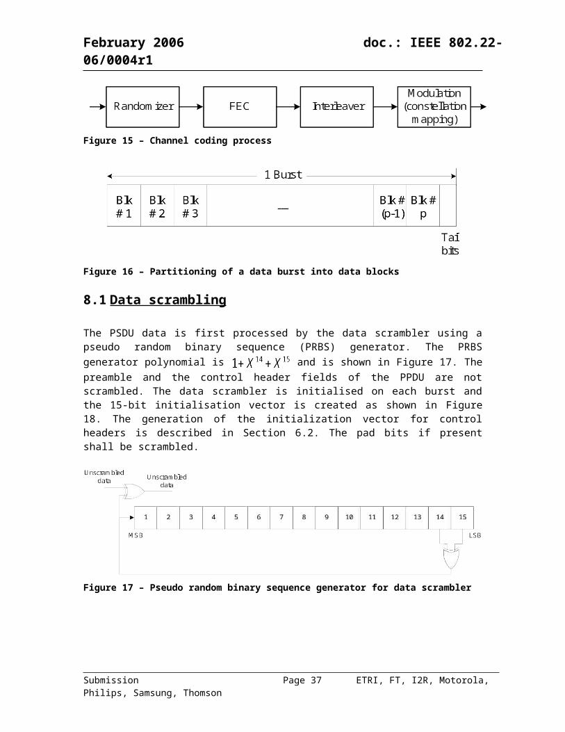
February 2006 doc.: IEEE 802.22-06/0004r1
(bytes)
18 27 18 24 18 24 27 36
24 36 24 36 48
30 60
36 36 36 36 72
Table 15: Possible data payload for one sub-channel
Modulation
schemeQPSK 8PSK 16-QAM 64-QAM Coded
Bytes
Encoding Rae ~1/2 ~2/3 ~3/4 ~5/6 ~1/2 ~2/3 ~1/2 ~2/3 ~3/4 ~5/6 ~1/2 ~2/3
Allowed Data
(Bytes)
6 9 1216 20 16 20 24
16 25 16 25 16 25 3623 35 23 35 4831 6040 40 40 40 72
Table 16: Code parameters for different coded block sizes
Data Bytes
Coded Bytes Constituent Code parametersIx Iy D Q
6 12 (8,7) (32,26) 4 8 0 69 12 (16,15) (16,15) 6 6 4 5
16 24 (8,7) (32,26) 2 0 0 220 24 (16,15) (16,15) 2 2 4 516 36 (32,26) (16,11) 11 2 6 725 36 (8,7) (64,57) 2 16 0 523 48 (32,26) (16,11) 4 2 8 635 48 (32,26) (16,15) 0 4 0 631 60 (32,26) (32,26) 10 10 4 440 72 (32,26) (32,26) 8 8 0 4
8.3 Bit interleaving
A two-step block interleaver shall be used to interleave the encoded and punctured data. The block size of the interleaver is determined by the parameter NCBPB (number of coded bits per encoded block, see Table 18). The first step of the interleaving process ensures that the adjacent coded bits are mapped onto non-adjacent sub-carriers in a sub-channel, while the second step of the interleaving process ensures that the adjacent coded bits are mapped alternately onto less or more significant bits of the constellation.
Let k, i, and j represent the index of the coded bits before the first permutation, after the first permutation and after the second permutation respectively. The first permutation is defined by the rule:
Submission Page 37 ETRI, FT, I2R, Motorola, Philips, Samsung, Thomson
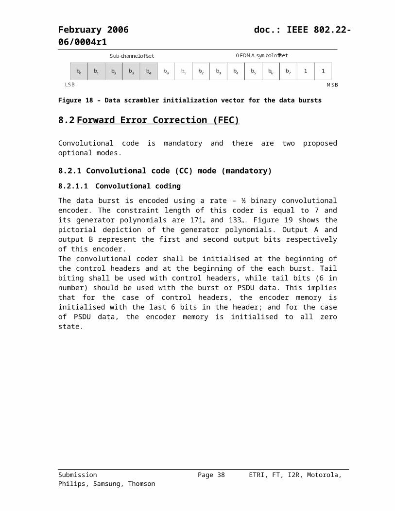
February 2006 doc.: IEEE 802.22-06/0004r1
The second permutation is defined by the rule:
The value of s is determined from the parameter NCBPC (see Table 17) and is given as
The parameter d is dependent on number of sub-carriers allocated per sub-channel. For the case of 48 sub-carriers per sub-channel, the value of d is equal to 16.
9. Constellation mapping and modulation
9.1 Transformed OFDMA modulation
9.1.1 Data modulationThe output of the bit interleaver is entered serially to the constellation mapper. The input data to the mapper is first divided into groups of NCBPC (see Table 17) bits and then converted into complex numbers representing QPSK, 16-QAM or 64-QAM constellation points. The mapping is done according to Gray-coded constellation mapping. The complex valued number is scaled by a modulation dependent normalization factor KMOD. Table 17 shows the KMOD values for the different modulation types defined in this section. The number of coded bits per block (NCBPB) and the number of data bits per block for the different constellation type and coding rate combinations are summarized in Table 18. Note that a block corresponds to the data transmitted in a single sub-channel.
Table 17: Modulation dependent normalization factor
Modulation Type NCBPC KMOD
QPSK 216-QAM 464-QAM 6
Table 18: The number of coded bits per block (NCBPB) and the number of data bits per block (NDBPB) for the different constellation type and coding rate combinations
Constellation type Coding rate NCBPB NDBPB
QPSK ½ 96 48QPSK ¾ 96 72
16-QAM ½ 192 9616-QAM ¾ 192 14464-QAM ½ 288 14464-QAM 2/3 288 19264-QAM ¾ 288 21664-QAM 5/6 288 240
Submission Page 38 ETRI, FT, I2R, Motorola, Philips, Samsung, Thomson
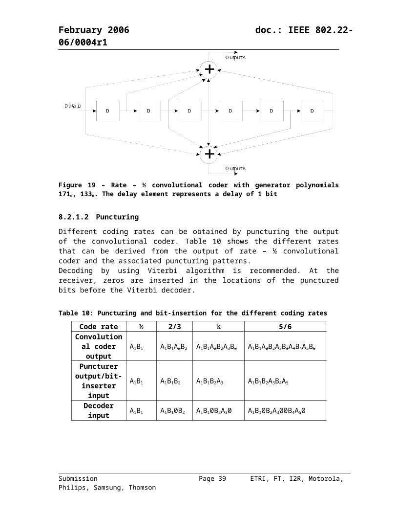
February 2006 doc.: IEEE 802.22-06/0004r1
9.1.1.1 Transformed OFDMA
In transformed OFDMA, a square transform matrix is used to spread each data to all the outputs of the transformation, which will be eventually sent to different sub-carriers. This transformation is beneficial in a fading environment since each data has been spread to all sub-carriers. It is still possible to restore the date even when some of the sub-carriers experience deep fade.An M x M matrix is used to spread the output of the constellation mapper. The type of the matrix to be used for different configurations is shown in Table 8. For purpose of spreading, the output of constellation mapper is grouped into a symbol block of M symbols that is corresponding to the bandwidth of CPE (uplink) or bandwidth for CPE (downlink). Each block is then coverted into parallel data and multiplied with a square transform matrix.The transformation is performed according to the following equation
,where X represents the constellation mapper output vector and is given as ,
S represents the transformed symbols and are defined as , and C (with size M x M) represents the transform matrix. The transform matrix shall be a unitary matrix with elements having constant amplitudes.Examples of the transform matrix include the Hadamard matrix, FFT matrix, rotated FFT matrix , frequency offset DFT matrix and Identity (no transformation) matrix.Hadarmard transformation matrix is given by the following Equation
,
where H1 = [1] and
Rotated FFT transformation matrix is given as:,
where and F is the FFT matrix of size M.The transform matrix may also be an identity matrix, when non-transform mode is selected.
The spreading matrix for SCH is defined in 6.2.1.
9.1.2 Pilot modulationThe pilots are mapped using QPSK constellation mapping. Spreading is not used on the pilots. The pilots are defined as
, and
10. Base station requirements
10.1Transmit and receive center frequency tolerance
The transmitter and receive center frequency tolerance should be within ±2 ppm.
Submission Page 39 ETRI, FT, I2R, Motorola, Philips, Samsung, Thomson
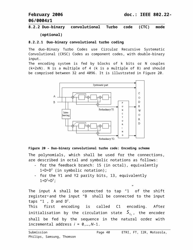
February 2006 doc.: IEEE 802.22-06/0004r1
10.2Symbol clock frequency tolerance
The symbol clock frequency tolerance should be within ±2 ppm.
10.3Clock synchronization
The transmitter center frequency and the symbol clock frequency should be derived from the same reference oscillator
11. Channel Measurements/Sensing
When channel measurement is mandated by the BS, CPEs shall make the required channel measurement. The channel measurements can range from simple received signal strength measurements (RSSI) or signal energy in a given TV band or frequency or the detection of the characteristics of the signal. The RSSI can be used for quality measurement of the signal from the BS station, or for detecting the presence of any other signal in a TV band. The measurement results are reported via ???? messages.
11.1Overall Sensing Scheme and Procedure
In this proposal, we suggest the spectrum sensing architecture shown in Figure 23. The sensing system comprised of (i) a wideband antenna, (ii) a wideband RF front-end for down converting received signal (iii) energy detection for determine candidate channels and (iv) find/feature detection for identifying the type of incoming signal and detecting low power signals.
MAC
Fine/Feature
RFE
Energy Detection
Omni Antenna
Control MAC
Fine/Feature
RFE
Energy Detection
Omni Antenna
Control
Figure 23 – Sensing architecture
The unoccupied channel selection is done by two step approach (shown in Figure 24) to meet the time and sensitivity requirement from the MAC. First, multiple unoccupied channel candidates are determined by energy detection method. The threshold can be set by BS or CPE. The swapping time is more important than the sensing sensitivity at this stage. This info is sent to
Submission Page 40 ETRI, FT, I2R, Motorola, Philips, Samsung, Thomson
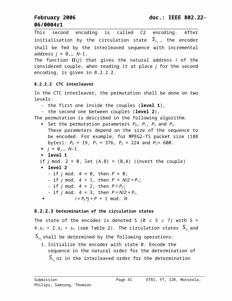
February 2006 doc.: IEEE 802.22-06/0004r1
MAC for selecting one candidate channel for communication. Then Fine/Feature sensing is performed for the selected channel for identifying the type of incoming signal. Also at this stage, very low power narrowband signal can be detected. If any signal is detected the given channel, then MAC will select another candidate channel for fine/feature detection until finding unoccupied channel.
Select candidates via Energy Detection
Fine/Feature detection for a selected channel
Select candidates via Energy Detection
Fine/Feature detection for a selected channel
Figure 24 – Sensing Procedure
Even, while in communication, the sensing block is working for finding other unoccupied channels, check if there is any attempt on the channel currently being used from a primary user and detecting the selected channel by request from base station for distributed sensing purposes. There could be many different type of detection method can be applied for the sensing block.
11.2Energy Detection
11.2.1 RSSI measurementThe RSSI measurement shall be reported in units of dBm. The actual implementation of the RSSI measurement is left to individual implementation. However, one possible method of implementation is by measuring the energy in a given band and converting that to the input signal strength using
where G is the RF front-end gain from antenna to ADC input in dB, Vc is the ADC input clip level, E2 is the measured signal power. The signal power, E2, can be estimated using various techniques and is left to the particular implementation. However in order to have good interoperability, the particular implementation need to result in a measurement that is similar to the value obtained using the following method. Assume the input signal in one TV band is
. Then, average this signal, y(k), over a window of K samples.
Then estimate the mean and variance of p(k) using a first-order low-pass filter as
Submission Page 41 ETRI, FT, I2R, Motorola, Philips, Samsung, Thomson
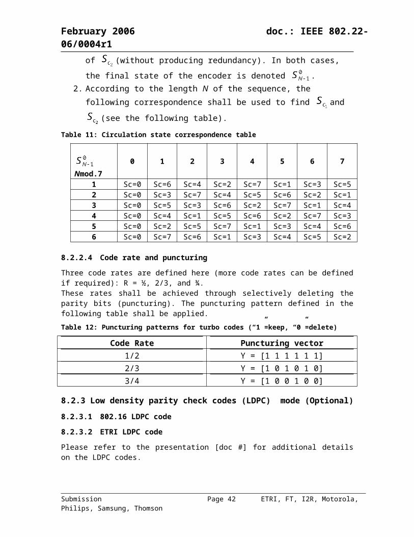
February 2006 doc.: IEEE 802.22-06/0004r1
where is the mean and is a constant set by the BS. The mean and variance are reported back to the BS upon request using the equation provided above for RSSI.
11.2.2 Multi-Resolution Spectrum Sensing The MRSS is suggested as a flexible energy detection based spectrum sensing technique. The wavelet transform is applied to the input signal and the resulting coefficient values stand for the representation of the input signal’s spectral contents with the given detection resolution. Figure25 shows the functional block diagram of the suggested MRSS technique. The building blocks consist of the analog wavelet waveform generator, the analog multiplier and the analog integrator for computing the correlation, and the low speed analog-to-digital signal converter (ADC) to digitize the calculated analog correlation values.
X ADC
v(t)*ejwct
Driver Amp CLK#2
Signal Processing
Timing Clock
Wavelet Generator
CLK#1
x(t)
w(t)
z(t) y(t)X ADC
v(t)*ejwct
Driver Amp CLK#2
Signal Processing
Timing Clock
Wavelet Generator
CLK#1
x(t)
w(t)
z(t) y(t)
Figure 25 – Functional block diagram of the MRSS
The wavelet pulse is generated and modulated with I-, Q-sinusoidal carrier with the given frequency. The correlations are calculated with the wavelet waveform with the given spectral width, i.e. the spectrum sensing resolution. By sweeping the local oscillator (LO) frequency with the certain interval, the signal power and the frequency values are detected over the spectrum range of interest. The resulting correlation with the I-, Q- components of the wavelet waveforms are digitized and their magnitudes are recorded. If these magnitudes are greater than the certain threshold level, the sensing scheme determines the meaningful interferer reception.Since the analysis is performed in the analog domain, the high-speed operation and low-power consumption can be achieved. By applying the narrow wavelet pulse and the large tuning step size of LO, this MRSS is able to examine the very wide spectrum span in the fast and sparse manner. On the contrary, very precise spectrum searching is realized with the wide wavelet pulse and the delicate adjusting LO frequency. By virtue of the scalable feature of the wavelet transform, multi-resolution is achieved without any additional digital hardware burdens. Moreover, unlike the heterodyne-based spectrum analysis techniques, this MRSS technique does not need any physical filters for image rejection due to the band pass filtering effect of the window signal.
Submission Page 42 ETRI, FT, I2R, Motorola, Philips, Samsung, Thomson
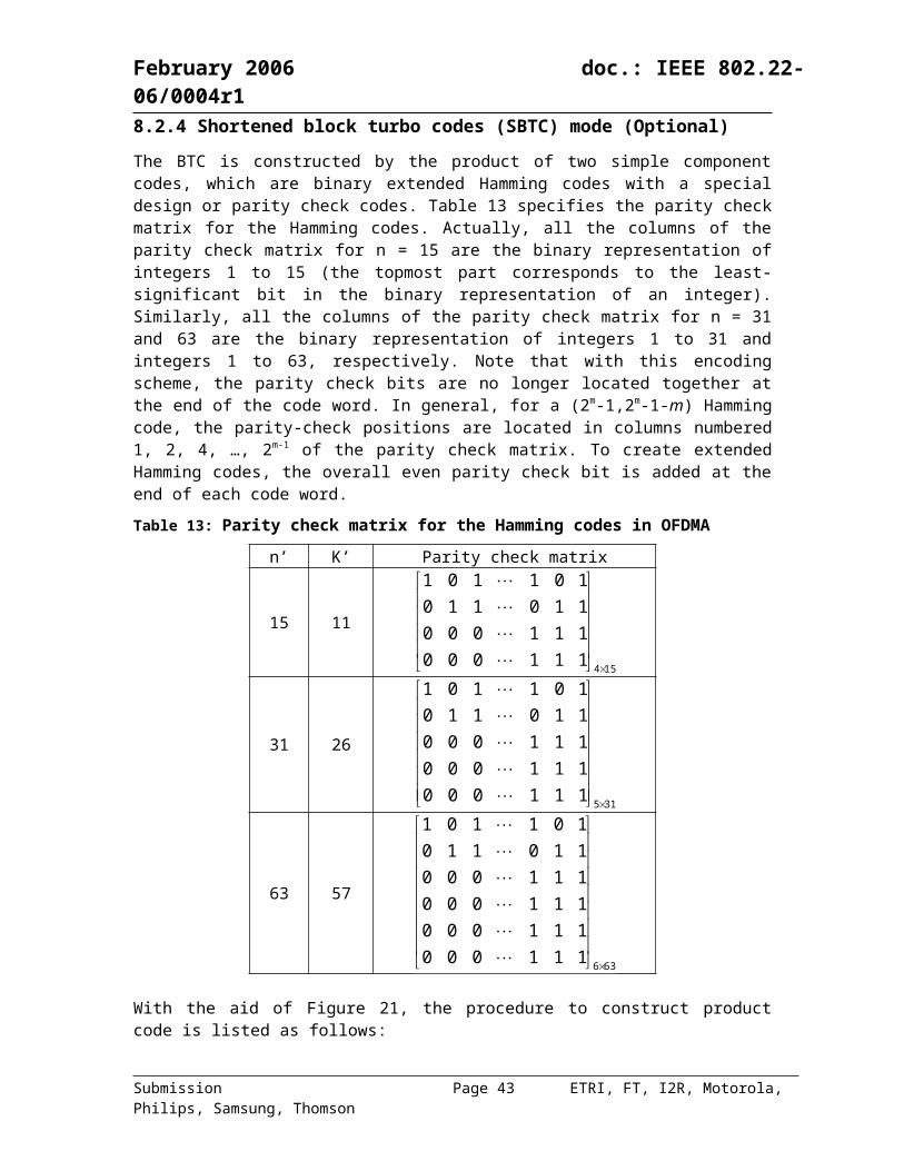
February 2006 doc.: IEEE 802.22-06/0004r1
11.3 Fine/Feature Detection
Upon request by the BS, the CPE shall perform signal detection in a given band. This would be from simple energy-based detection to detecting a specific feature of the signal.
11.3.1 Fine Energy-based detection:Energy based detection is simply comparing the energy estimated by using the above method to a threshold. The energy-based detection shall perform the following
,
where c is a constant and in the noise power of the RF input. The noise power can simply be estimated form the thermal noise adjusted for any other gain of the RF front-end. Alternatively, the CPE can also periodically estimate its input noise power using a vacant channel or by disconnecting the antenna. The CPE shall also report the confidence of this detection [TBD]. The BS shall provide adequate time for estimating the energy.
11.3.2 Signal Feature DetectionUpon request by the BS, the CPE shall identify the type of the signal seen at its input, example ATSC TV, DVB-T, Part 74 devices. The following subsections describe some of the method to be used for this signal feature detection.11.3.2.1 Part 74 Devices.
Part 74 Devices (wireless microphone) occupy only a small portion of the TV spectrum. This fact is used to detect if there is enough energy in a part of a spectrum as follows:First, an FFT operation is performed on the input signal as follows
where Y(k,m) is the k’th block FFT, rn is the received data and N is the size of the FFT (N=2048 for one TV channel). Generally, rn is composed of the noise and the narrower-band signal to be detected. After performing the FFT, the received power spectrum is then computed and averaged over each freq bin
Where K is set by the BS. Further spectral averaging is performed by filtering this estimate, P(k,m), with the expected spectrum of the signal being detected. In the presence of frequency selective multipath between the detecting device the transmitter of the signal being detected, the expected spectrum is not known. Then, a simple rectangular filter with bandwidth equal to the bandwidth of the signal can be used. The mean and a modified variance are computed using
Submission Page 43 ETRI, FT, I2R, Motorola, Philips, Samsung, Thomson
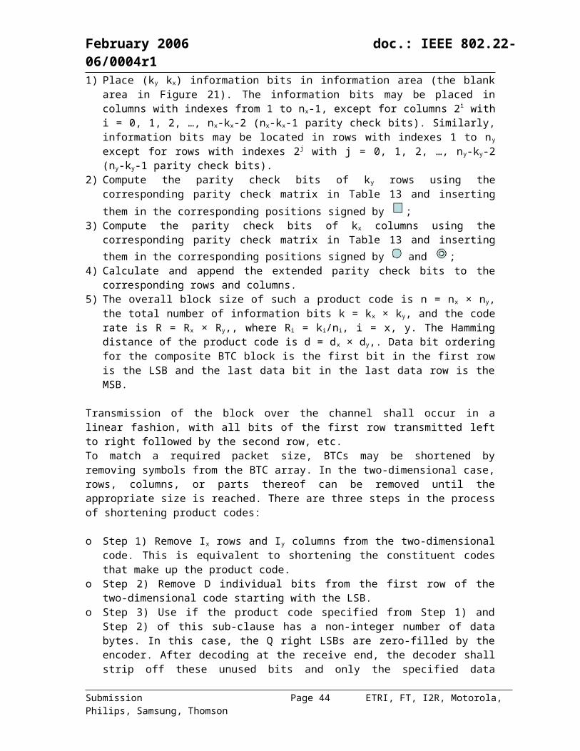
February 2006 doc.: IEEE 802.22-06/0004r1
The generalized detection method is described below.
where and constants set by the BS.
11.3.2.2 ATSC DTV Detection
The proposed technique here is based on correlating the received signal with a copy of a known reference signal. For US DTV, this will be the PN511 sequence. After the necessary frequency correction, the CPE shall correlate the input signal with the known PN511 sequence as.
A running mean and variance of this correlation output is computed using
where the filter parameters are set by the BS. When the correlation output is random, then the mean and variance are identical. However, if the output is not random (such as when field sync is present and a sample of p(k) exhibits a value very different from the normal range (example, a peak), then the variance will respond faster than the mean. An ATSC DTV is declared detected when
where k’ is the sample where the peak sample is shown in p(k) and c is constant set by the BS.
In ATSC DTV signals, there are also three PN63 sequences concatenated together in the data field sync segments. The three sequences are the same except that the middle sequence inverts on every other data field sync. These specific features can be employed for detection of ATSC DTV signals. One method utilizing PN63 sequences is given in Figure 26. Peak detection is performed on y1 and y2: if there is an outstanding peak appearing in either y1 or y2, we make a decision that the ATSC DTV signal is present. Alternatively, we can compute the maximum value between the absolute value of y1 and y2, i.e., y = max(|y1|, |y2|), and use y for peak detection.
Figure 26 – ATSC DTV feature detection using PN63 sequences
Submission Page 44 ETRI, FT, I2R, Motorola, Philips, Samsung, Thomson
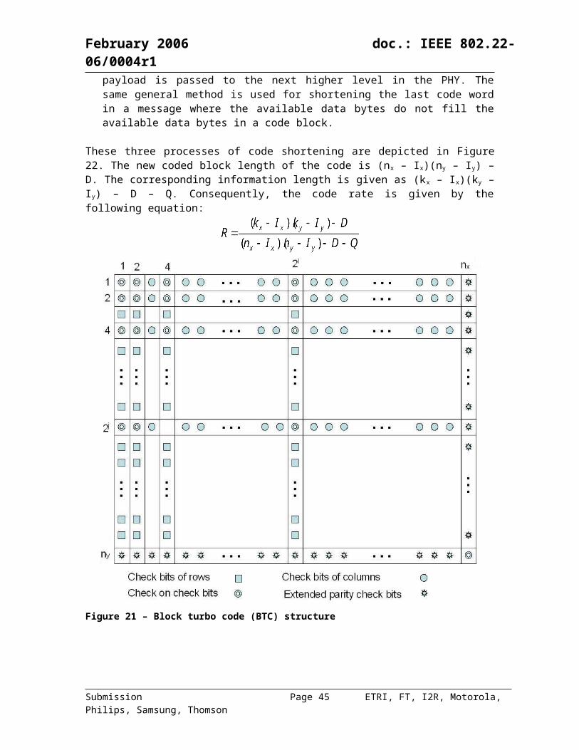
February 2006 doc.: IEEE 802.22-06/0004r1
In ATSC DTV signals, a two-level (binary) four-symbol data segment sync is inserted at the beginning of each data segment. A complete segment consists of 832 symbols: four symbols for data segment sync, and 828 data symbols. The data segment sync pattern is a 1001 pattern. Multiple data segments (313 segments) comprise a data field. The data segment sync can also be utilized for ATSC DTV signal detection especially when the carrier recovery is problematic in low signal-to-noise situations.In order to achieve a robust detection of the segment sync, a delay-line structure is used as in Figure 27. The signal is multiplied by a delayed, conjugated version of itself. The result is summed by a sliding window filter of length four symbols: the conjugation ensures that any carrier offset will not affect the amplitude following the sliding window filter. The output of the sliding window filter is processed using an IIR filter in order to improve the robustness of the detection over multiple segments. The IIR filter is a leaky integrator having a delay line equal to the segment length (Alternatively, an integrate-and-dump approach might be used).
Figure 27 – Segment Sync Detector
Denote the output of the IIR filter as z(k), similarly as PN511 detection, a running mean and variance of z(k) can be computed, given as
An ATSC DTV is declared detected when
Where and are system parameters set by the BS.
11.3.2.3 Synchronization Method using Strong DTV Signals
ATSC DTV detection performance can be improved by increasing the accuracy of either the timing or carrier frequency references in the receiver. One way to implement this at the receiver is by receiving a strong station on another frequency, and observing the timing and frequency offsets and settings relative to its known timing and frequency characteristics. These observed timing and frequency offsets and setting can then be used to calibrate the receiver, such that a DTV station can be sensed with accurate knowledge of its timing and frequency location.As specified in ATSC A/54A ATSC Recommended Practice, carrier frequencies are specified to be at least within 1 KHz, and tighter tolerances are recommended for good practice. ATSC DTV channels will be on specific frequencies, depending on the NTSC and ATSC interferers in the location. This allows 14 possible carrier offsets for a given channel. As NTSC transmission is discontinued, the number of channel offsets should decrease to two, with a tolerance of 10 Hz.
Submission Page 45 ETRI, FT, I2R, Motorola, Philips, Samsung, Thomson
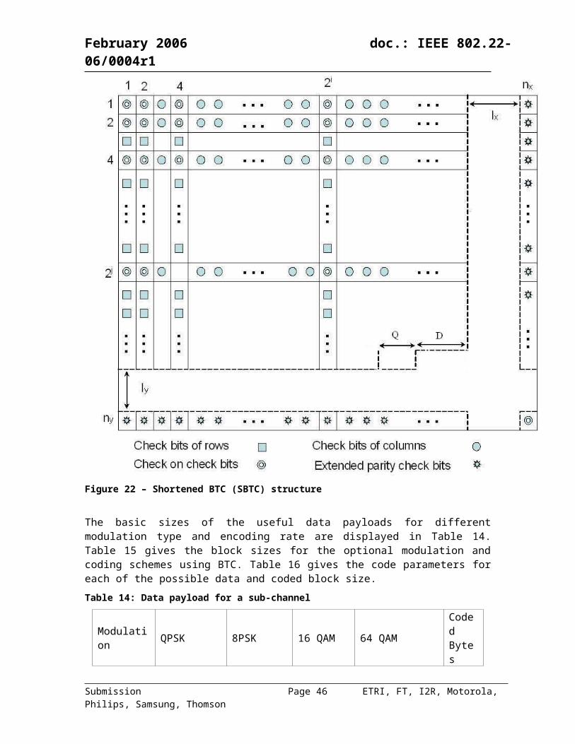
February 2006 doc.: IEEE 802.22-06/0004r1
This method relies on the short-term stability of the frequency reference in the receiver. Stability of the tuner local oscillator would be a consideration in the design of the tuner for a receiver using this approach. To get a close frequency reference for detecting the presence of an ATSC signal, this system tunes in an existing ATSC signal. With this signal as a reference, the tuner local oscillator PLL conversion ratios are noted, and the frequency offset is stored. If an analog AFC is used, this voltage is frozen via a track and hold or by freezing the DAC which generates the control voltage. This will keep the reference oscillator of the tuner PLL at as constant of frequency as possible. Typical tuners allow frequency selection as a multiple of a step size between 50 and 200 KHz.A numerically controlled oscillator (NCO) is used to fine-tune the signal. Once a channel at the nearest synthesizer step is established, the NCO is tuned to lock to the channel using known carrier recovery techniques. This information is recorded and used to estimate the PLL reference frequency or synthesizer step. This is illustrated in the equation below, where Fc is the channel frequency (Low band edge from Figure 30 plus low band edge offset from Table 19), n is the PLL divider, Fstep is the PLL frequency step, and Foffset is the NCO measured deviation from the PLL frequency step. Foffset includes both the distance from the multiple of Fstep to the channel and the error caused by frequency differences in the local frequency reference and the transmitter frequency reference. Since we measure Foffset, we know n and Fc, we can solve for Fstep to determine the exact frequency of another ATSC channel.
An analog oscillator could be used, but we benefit from the digital design in having a precise (as stable as the sample clock) measurement of carrier frequency offset from the PLL synthesizer step. Figure 28 illustrates the NCO and de-rotator in the context of a DTV tuner, receiver, and detector. The detector is the device which is used to find ATSC signals by correlating with the training signals.Determining the reference oscillator frequency can be achieved in multiple ways. First, if only one strong DTV signal is present, one will assume that the DTV signal is one of the 14 possible frequencies listed in ATSC A/54A (See Figure 30 & Table 19). Solving for the reference oscillator frequency or PLL frequency step, we can find 14 possible reference oscillator frequencies or frequency steps. After NTSC is made obsolete, the number of possible frequencies will be reduced to two (Boldface in table). Second, if multiple DTV channels are present, one can solve for the best fit of the frequency step, providing precise frequency information, possibly even determining the exact reference oscillator frequency rather than a set of guesses. Once this is accomplished, the channel under test is selected, and the de-rotator oscillator is tuned to try each of the possible channel frequencies (This could be combinations of reference frequency estimates, and channel frequency possibilities -- a worst case of 196 combinations, or fewer if some of the close entries are considered one entry). If the ATSC detector finds evidence of an ATSC signal, the channel is presumed to have a DTV signal, even if that signal is below the usable signal strength. The target sensitivity for this device is to detect ATSC signals with a signal strength of -116dBm. This is >30dB below the threshold of visibility. The ATSC detector will perform repeated correlations of the training signals of the ATSC signal, to bring the low level signal out from the noise floor. By removing carrier offsets to the order of 1 KHz, ATSC detection methods introduced in previous sections should reveal the presence of ATSC signals below the noise floor. Once NTSC is obsolete, the limited number of frequency possibilities will reduce the number of combinations of reference frequency estimates and channel frequency possibilities to 4.
The algorithm flow is illustrated in Figure 29.
Submission Page 46 ETRI, FT, I2R, Motorola, Philips, Samsung, Thomson
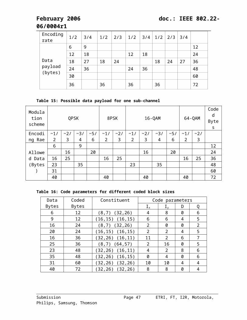
February 2006 doc.: IEEE 802.22-06/0004r1
Since this is an open loop timing system, it is important to periodically check timing with the reference station, depending on the drift characteristics of the reference oscillator and to a lesser extent, the sample clock oscillator. It is also possible to use two synchronized tuners to constantly lock to a DTV channel while looking for other DTV channels.
Figure 28 – ATSC Alternate Channel Carrier Frequency Reference
Submission Page 47 ETRI, FT, I2R, Motorola, Philips, Samsung, Thomson
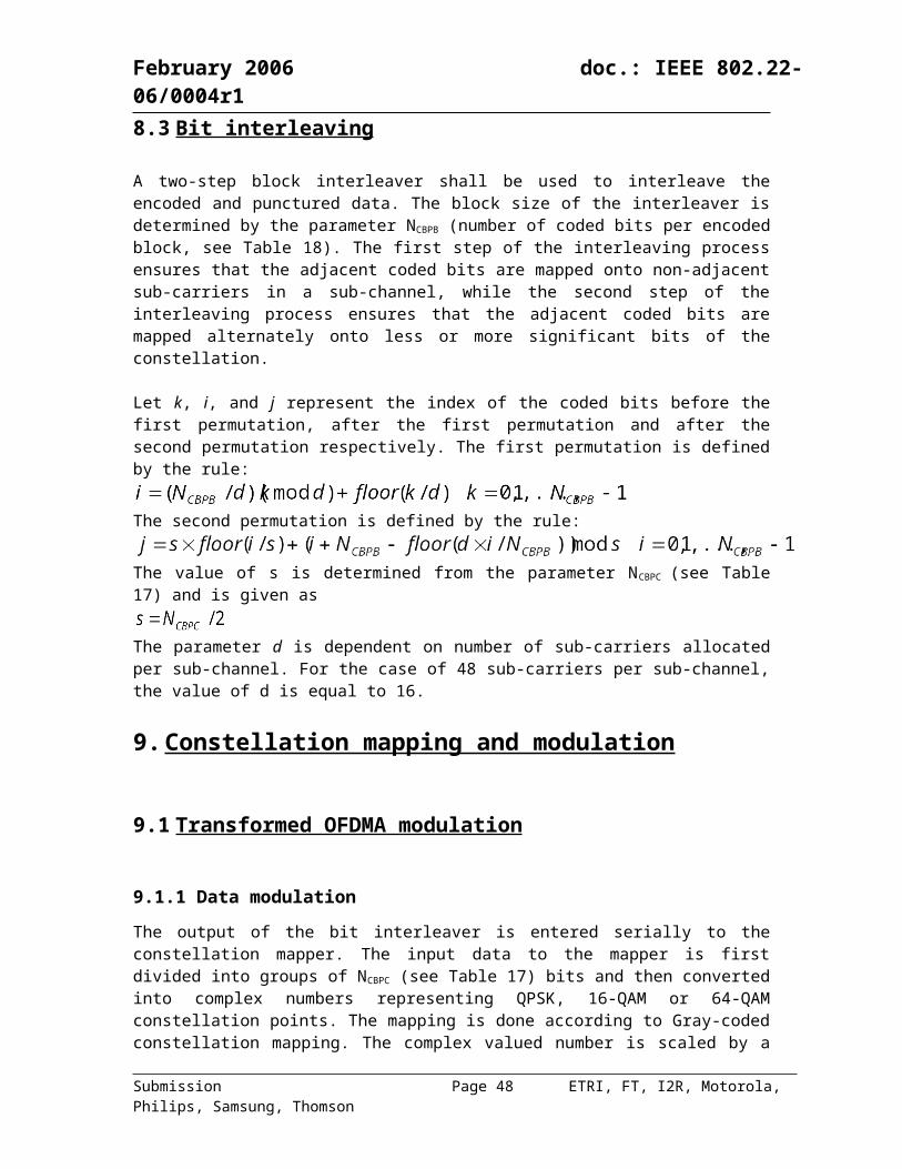
February 2006 doc.: IEEE 802.22-06/0004r1
Figure 29 – Flowchart for synchronization using strong DTV signals
Submission Page 48 ETRI, FT, I2R, Motorola, Philips, Samsung, Thomson
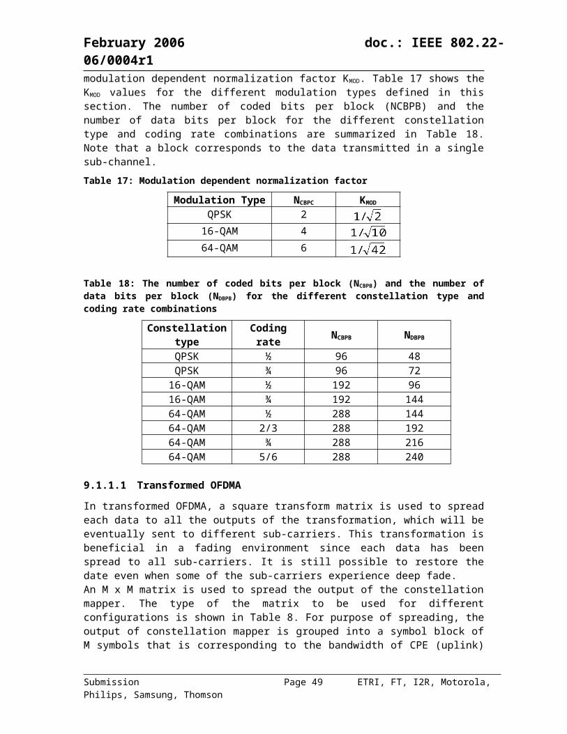
February 2006 doc.: IEEE 802.22-06/0004r1
Figure 30 – TV Channel Frequencies
Table 19: Frequency of Pilot Tone with respect to low band edge of channel
Low Band Edge Offset in
Hz
Tol. ±Hz
Condition
309440.559 10 Standard DTV322138 3 Lower Adjacent NTSC with -10 KHz Offset328056 1000 Co-channel NTSC with -10 KHz Offset
328843.6 10 Co-channel DTV332138 3 Lower Adjacent NTSC338056 1000 Co-channel NTSC341541 10 Co-channel DTV with DTV with Lower Adjacent NTSC with -10 KHz offset342138 3 Lower Adjacent NTSC with 10 KHz Offset347459 1000 Co-channel DTV with DTV with Co-channel NTSC with -10 KHz offset348056 1000 Co-channel NTSC with 10 KHz offset351541 10 Co-channel DTV with DTV with Lower Adjacent NTSC357459 1000 Co-channel DTV with DTV with Co-channel NTSC361541 10 Co-channel DTV with DTV with Lower Adjacent NTSC with 10 KHz offset367459 1000 Co-channel DTV with DTV with Co-channel NTSC with 10 KHz offset
Submission Page 49 ETRI, FT, I2R, Motorola, Philips, Samsung, Thomson
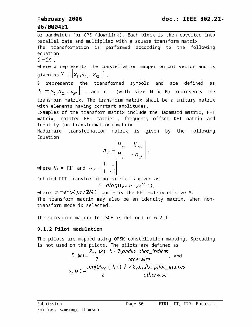
February 2006 doc.: IEEE 802.22-06/0004r1
11.3.3 Cyclo-Stationary Feature DetectionCommunication signals have traditionally being modeled as stationary. A large class of signals like AM, FM, VSB, PSK, QAM, OFDM, CDMA in fact exhibit underlying periodicities in their signal structure. The scheme described herein aims to exploit these signal properties to detect and classify signals, and is based on the theory of cyclostationarity. Consider a zero-mean discrete-time signal . We say that is cyclostationary with period
if its autocorrelation function is -periodic, i.e.
We define the cyclic autocorrelation function (CAF) as
with the discrete time Fourier transform giving the cyclic spectrum density (CSD), also known as the spectral correlation function (SCF), defined as
The parameter is called the cycle frequency; each cyclic frequency is an integer multiple of the fundamental time period of the signal. Note that for , the CAF and CSD reduce to the conventional autocorrelation and power spectral density functions. Also, due to the symmetry and periodicity in , the entire function is completely specified over
. Further we note that a cyclostationary signal passed through a
linear time-invariant channel, which the channels in [2] are modeled by, remains cyclostationary. Also, if the signal is composed of signals , i.e.
where signal has cycle frequency , we can extract the CSD from by considering the particular cycle frequency , i.e.
.Different signals exhibit different underlying signal periodicities, i.e. exhibit distinct spectral characteristics at their cycle frequencies. For a large class of signals, we can determine what the cycle frequency is. We now consider a simple example of a BPSK signal and specify its cycle frequency. Consider the BPSK signal
where is the average power, the IF carrier frequency, the bit duration and a random message sequence. One can easily derive the expression for the CSD to show that it has spectral components at , for integer . Thus to detect a BPSK signal with known characteristics, one only has to analyze the CSD at .To gain an intuition into how cyclostationarity based detection works, let us revisit the problem of binary hypothesis testing. We want to determine whether the signal of interest to be detected
, that is transmitted over a channel with channel impulse response in the presence of
Submission Page 50 ETRI, FT, I2R, Motorola, Philips, Samsung, Thomson
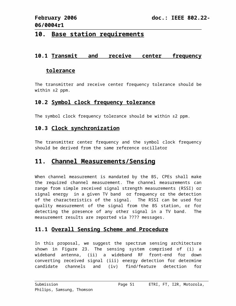
February 2006 doc.: IEEE 802.22-06/0004r1
additive white Gaussian noise (AWGN) , is present or not on the basis of the measured received signal . That is, we want to determine which of the following hypothesis is true:
It is easy to show that we have the following relation
The conventional energy detector corresponds to testing the energy levels obtained from at for the signal absent and signal present cases. When the signal is heavily attenuated and/or is in the presence of a strong noise component, it becomes difficult to discriminate between the energy levels of signal+noise and noise. However a cyclostationary detector is not faced with this problem since detection can theoretically be done irrespective of the noise power level. Different forms of detection statistics are possible, each derived from . Some examples areSingle-cycle magnitude detector:
where is the sliding cyclic auto-periodogram and the
observation window length.Multi-cycle magnitude detector:
This is simply a detector, , that is evaluated over all or a set of cycle frequencies.
In fact, we can also consider one-dimensional processing to alleviate some of the computational burden that arises from two-dimensional processing by projecting on the cycle frequency
axis to obtain the projection .
11.3.4 Detailed requirements on signal detection Even without using distributing sensing, there are already several possibilities to detect an incumbent thanks to the spectrum density:
threshold on the signal energy in a sub-band threshold on a pilot frequency or on several pilot frequencies threshold on a correlation between the spectrum received and a known signature
The more general method is the correlation between the spectrum received and a known signature, it is know in the literature under the name Optimal Radiometer. This is however not the purpose of this document to discuss these methods. However, some further details are needed to deeply specify the expected performance of the signal detection.The detailed requirements for the signal detection are as follows:
Submission Page 51 ETRI, FT, I2R, Motorola, Philips, Samsung, Thomson
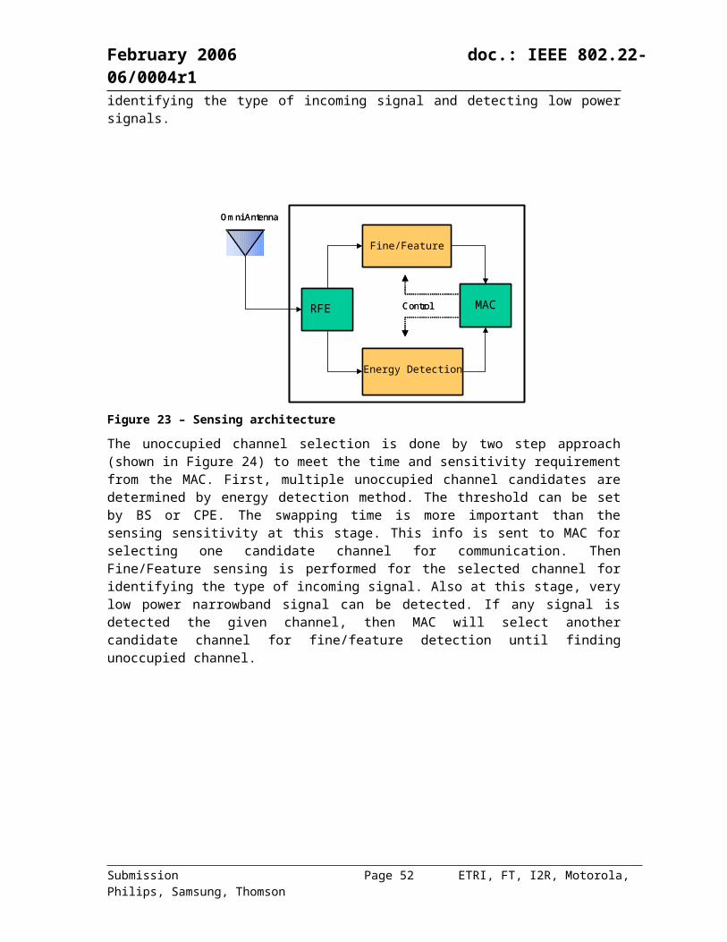
February 2006 doc.: IEEE 802.22-06/0004r1
Gaussian channel and multipath channel. The effect of multipath channel on the ATSC and NTSC signal are given by the document WRAN channel modelling IEEE802.22-05/0055r7. (The approximation of quasi-static channel is valid because the sensing period is short compared with the inverse of the Doppler frequency).
The video carrier (NTSC) or the digital pilot frequency (ATSC) are in different offsets in the 6 MHz. However, the maximum offset deviation is 10 kHz in comparison to the nominal values. According to the Shared Spectrum Comments, Appendix A to Federal Communications Commission, "In the Matter of Unlicensed Operation in the TV Broadcast Bands Additional Spectrum for Unlicensed Devices Below 900 MHz and in the 3 GHz Band", ET Docket No. 04-186 and ET Docket No. 02-380, the carrier and pilot can be set to:
o The “standard” frequency
o 10 kHz above the “standard” frequency
o 10 kHz below the “standard” frequency.
o Low power analog TV stations have different rules. Apparently they can put their video carrier anywhere between minus 10 kHz and plus 10 kHz in relation to the standard carrier frequency
Noise Figure is set to zero. A simple shift from the Noise Figure level on the energy of the ATSC signal or peak of the NTSC carrier can be done for the test requirements.
12. Control mechanisms
12.1CPE synchronization
All the CPEs will be synchronized with the BS using the superframe preamble. It is required that all the US transmissions will be received at the BS within 25% of the minimum guard interval. We propose to define a two-step synchronization process: an initial (coarse) synchronization phase and a fine synchronization based on the ranging procedure.
12.1.1 Initial synchronizationThe initial synchronization process provides the CPE with a minimum time and frequency accuracy to enable it to recover the ranging information. The purpose of the initial synchronization is to provide to the CPE:
The time of the next upstream transmission frame;
The information to initiate its internal clock and reach the required time and frequency accuracy.
12.1.2 Carrier synchronizationDuring this phase, the CPE can synchronize the carriers in phase and frequency to the RF upstream channel by using phase locked techniques to synchronize the local oscillator driving the CPE to the reference clock transmitted by the Base Station.
Submission Page 52 ETRI, FT, I2R, Motorola, Philips, Samsung, Thomson
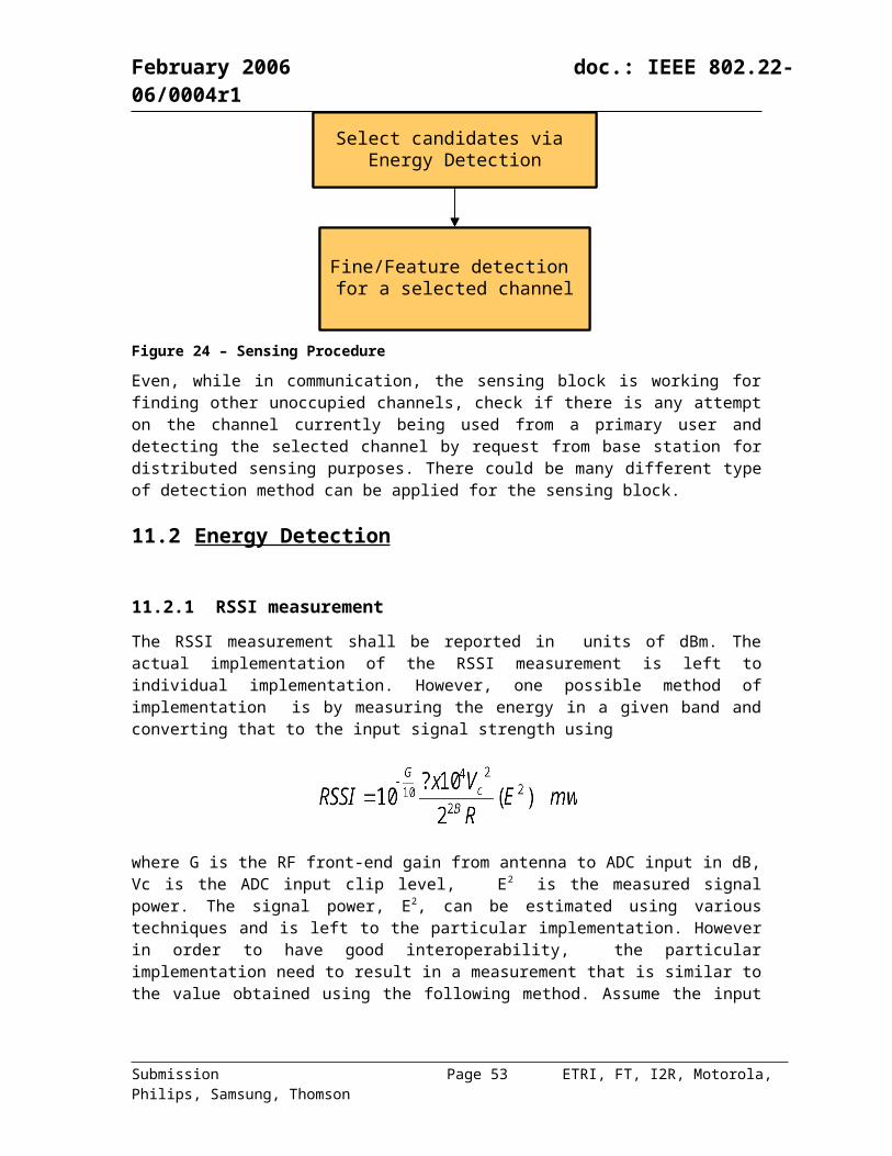
February 2006 doc.: IEEE 802.22-06/0004r1
12.1.3 Targeted tolerancesTable 20 sums up, for different encoding rates, the experimental (and theoretical) tolerances on the return channel transmitter characteristics:
Time (t);
Frequency (f/Cs);
Synchronization accuracy (A).
Table 20: Tolerance in time, frequency and synchronization for different coding rates. Ts= Symbol duration, Cs= Carrier spacing
Coding rate no coding 3/4 2/ 3 1/2t ± Ts/10 ± Ts/6 ± Ts /6 ± Ts/5
f/Cs ± 0.03 ± 0.04 ± 0.05 ± 0.075A 20 dB 17 dB 17 dB 20 dB
12.2Ranging
12.3Power control
13. Multiple Antenna Options
It is well known that the robustness, data-rate and/or range of a WRAN system can be improved by the use of multiple antennae at either the transmitter or the receiver or both. Multiple antennae techniques are optional in this proposal. The following methods of multiple-antenna usage are under consideration at this time.
13.1Equal Gain, Explicit Beamforming Using Codebooks
When multiple antennae are used for transmission, it is desirable to have each antenna transmit the same power. Traditional eigenvector based methods do not guarantee equal gain transmit vectors when the number of transmit antennae are greater than the number of transmitted streams. In OFDM transmission in particular, each power-amplifier is peak power limited and hence a beamforming solution that satisfies equal power/antenna in addition to the total power constraint is needed.
Let us assume a multiple-antenna system with NT transmit antennae and NR receive antennae. We will assume that there is only one data stream being transmitted, and that the beamforming vector is defined to be Q. Then the signal model is:
Submission Page 53 ETRI, FT, I2R, Motorola, Philips, Samsung, Thomson
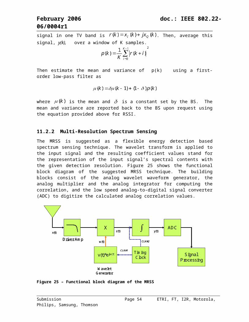
February 2006 doc.: IEEE 802.22-06/0004r1
where the received vector r is a NRx1 vector, the channel matrix H is a NRXNT matrix, the beamforming vector Q is a NTX1 vector and x is the data symbol. The transmitted vector is
, which is a NTX1 vector. In an OFDM system, the above signal model is repeated for each frequency bin. In a frequency selective channel, H and Q would be different for each frequency bin.
Let be the SVD decomposition of the channel matrix H. Then, it can be shown that the optimal choice for Q is where Vi is the ith column of matrix V. The requirement of equal gain means that the transmitted power from each antenna should be the same i.e. each element of the beamforming vector Q should have the same power. The optimal choice does not ensure that this is the case.
This proposal ensures equal transmitted power from each antenna by limiting all entries of Q to be , with the first entry being fixed at , i.e. Q is of the form [ ,…………]T. Thus, each beamforming vector can be specified with only 2(NT-1) bits. For a 2x1 beamforming system each beamforming vector will require only 2 bits to be specified.
For each frequency bin i, the beamforming vector Qi is picked to maximize from the possible choices for Qi. The total number of bits needed to specify
the beamforming vectors for Nf frequency tones is then 2* Nf *(NT-1).
If the subchannelization scheme uses multiple contiguous frequencies, then the number of feedback bits can be reduced by grouping p frequencies together and calculating a single
beamforming vector Q for this group that maximizes . Thus the number of
feedback bits can be reduced by a factor of p. For example, if each CPE is allocated 64 frequency tones and the channelization uses groups of 4 tones across the frequency band, a 4x1 beamforming system will require only 12 bytes of feedback to specify all the beamforming vectors and a 2x1 system will require only 4 bytes of feedback. The transmitter does not need to do any interpolation among the p frequencies: it applies the Q feedback directly to the data stream.
The above description was for one data stream. Quantized equal gain beamforming matrices can be formed using the same codebook for 2 or more data streams, .eg. a 4x2 system transmitting 2 data streams.
13.2Downlink Closed-Loop Space Division Multiple Access (CL-
SDMA)
The CL-SDMA modes can be used to enhance the throughput of medium to high SNR users, by simultaneously transmitting to N users in the same sub-channel, where N denotes the number of base station antennas. Since the WRAN channel is very slowly fading, reliable knowledge of the channel matrices can be obtained at the transmitter without excessive burden on feedback and signalling requirements. The CL-SDMA techniques can be applied on sub-channels when adjacent sub-carrier permutation is used and under the assumption that the channel is coherent within a sub-channel.
Submission Page 54 ETRI, FT, I2R, Motorola, Philips, Samsung, Thomson
February 2006 doc.: IEEE 802.22-06/0004r1
The following sub-sections describe two modes of CL-SDMA schemes. Both these modes require the CPEs to estimate their downlink channel matrices. This is provided by default on a downlink frame to allow for coherence demodulation. On-demand downlink sounding pilots or sequences could be provided to support a more flexible operation. Scheduling of users on the downlink at the base station is also assumed to be implemented, in order to select users that are suitable for the proposed modes. In general, if the channel matrices of users were rank-deficient, as would mostly be the case in the WRAN, a scheduling algorithm that exploits multi-user diversity would be able to select 2, 3 or 4 users with uncorrelated channels without much difficulty and complexity. It is also assumed that channel quality information (CQI) on short-term conditions of the channels of the users is provided to the base station through other means supported by the default operation in single antenna systems.
13.2.1 CL-SDMA Mode 1: Using FDD or TDD with 2 Base Station Antennas and Multiple Antennas at the CPEs
When the base station is equipped with two transmit antennas, CL-SDMA mode 1 also allows operating in FDD or TDD without relying on channel reciprocity, or when the CPEs have a single RF transmit chain. In TDD mode, it can be used either with channel reciprocity, or with the feedback procedure described in the next sections. CPEs must be equipped with at least two receive antennas. Two CPEs are served simultaneously by the base station. They will be referred as CPE 1 and CPE 2 in the sequel.
13.2.1.1 Transmitter and Receiver Structure
Figure 31 and Figure 32 show the linear processing operations required at the transmitter and at the receivers of each of the two active CPEs on a given sub-carrier. Operations are carried out in the frequency domain.
Channel Encoder
QAM Modulation X
X +
+
OFDMModulation 1
Channel Encoder
QAM Modulation X
XOFDM
Modulation 2
User 1Data Packet
User 2Data Packet
M1,1
M1,2
M2,1
M2,2
Figure 31 – Transmitter structure for CL-SDMA mode 1
Submission Page 55 ETRI, FT, I2R, Motorola, Philips, Samsung, Thomson
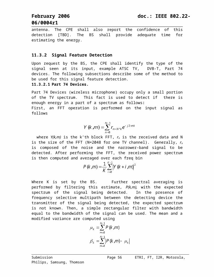
February 2006 doc.: IEEE 802.22-06/0004r1
1
2
OFDMDemodulation X
+
W*k,1
OFDMDemodulation X
W*k,2
NOFDM
Demodulation X
W*k,N
Channel Decoder
User k decodedData Packet
MMSE or ZF per tone
Figure 32 – 2 Receiver structure of User k for CL-SDMA mode 1
13.2.1.2 Preliminary Computation Phase at the CPEs
Users 1 and 2 perform the following operations (for conciseness, we only present the case of one user, denoted as user k): User k has an estimate of the downlink channel matrix . Each row of the matrix represents a CPE receive antenna. This estimate can represent the channel of a single sub-carrier, or of a group of adjacent sub-carriers. Depending on the case, the following operations apply to an individual sub-carrier, or to a group of adjacent sub-carriers. User k computes the following matrix (* denotes the transpose conjugate operation):
The elements of are represented as:
and , with degrees.
, with degrees and .
.Two codebooks are stored at the CPEs, and the same codebooks are stored at the base station. The first codebook quantizes and using B bits. The second codebook quantizes using B’ bits.Equivalently, values of can be stored in the codebook. Uniform quantization of the angles with a finite number of bits provides good performance. B=5 bits and B’=6 bits provide robust performance over a wide range of channel conditions, and closely approaches the performance with unquantized channel state information. Thus the channel state information of each user can
Submission Page 56 ETRI, FT, I2R, Motorola, Philips, Samsung, Thomson

February 2006 doc.: IEEE 802.22-06/0004r1
be reliably stored and conveyed using two bytes. The number of bits can be traded-off for performance.
13.2.1.3 Feedback of Channel State Information to the BS
Each CPE sends 2B+B’ bits to the base station through a robust feedback channel. For better performance, more than 2 CPEs are required to do so, so that an algorithm can optimize the spatial scheduling of users, using additional information such as signal to noise plus interference ratio monitored by the base station. In practice, it is recommended to feedback 2B+B’ bits per group of adjacent sub-carriers to limit the amount of feedback, and still provide a robust solution.
13.2.1.4 Computation Phase at the Base Station
Using the finite-rate quantized feedback received from the users, the base station performs the following operations: It first recover , , and for users .It is recommended that the same index feedback from both users should lead to slightly different values of the recovered values. This can be easily achieved by shifting the values represented by the entries in the codebook by a small amount (smaller than the resolution of the codebook) in order to avoid undesirable numerical effects that could occur in rare special cases. For example, if both users feedback the same index n representing the angle x, one user would use and the other user , where is smaller than the resolution of the codebook in the domain.In TDD operation with channel reciprocity, the base station directly obtains estimates of ,
, and for users .Then the base station computes:
and
and
and
Finally and .
Submission Page 57 ETRI, FT, I2R, Motorola, Philips, Samsung, Thomson
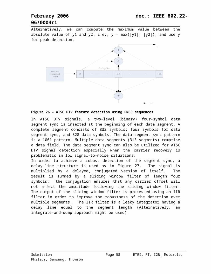
February 2006 doc.: IEEE 802.22-06/0004r1
and are the transmit filters used by the base station for users 1 and 2 respectively. We
express then explicitly as vectors with complex elements:
and
13.2.1.5 Downlink Data Transmission and Sounding
In the sub-channel with adjacent permutation sub-carriers, data symbols and downlink sounding pilots symbols are transmitted within the same sub-channel. The pilot symbols are used to transmit training data by beamforming with the transmit filters. At least one pilot must be sent to each user within a sub-channel. In practice, multiple pilots are used for each user. The pilots of users 1 and 2 are not transmitted on the same sub-carrier and OFDMA symbol. However the data symbols of users 1 and 2 are transmitted using their respective transmit beamforming vectors in the same sub-carriers and OFDM symbol.The pilots present in the traffic channel of a downlink frame with the adjacent permutation sub-carriers need to be reallocated for the purpose of downlink sounding. Their number and position can be adaptively selected, depending on channel conditions. On a pilot resource (time t and sub-carrier s), user k receives:
or
On every other (data) resource (time t and sub-carrier s), user k receives:
where is the power of the transmitted pilot, is the known training symbol, is the
channel matrix of user k at time t and sub-carrier s, and is additive noise and interference,
and are the data symbols sent to users 1 and 2 respectively. The properties of transmit and receive filters allow the receiver to completely remove the inter-user interference, or to mitigate it in the presence of practical impairments.
13.2.1.6 CPE Receiver Downlink Detection
The CPEs estimate their effective channel vector (which includes the transmit beamforming vector) using a procedure similar to the one they would use to estimate the downlink channel when transmit beamforming is not used. This can be done with interpolation in the time and frequency directions. This way, on each sub-carrier (recommended), or to represent a group of sub-carriers, each user builds an estimate of:
for ( is a normalization factor).
User k can directly use to detect its received data symbols. For improved robustness to channel variations, estimation imperfections, feedback delay and numerical effects, user k can form the MMSE filter on sub-carrier s:
Submission Page 58 ETRI, FT, I2R, Motorola, Philips, Samsung, Thomson
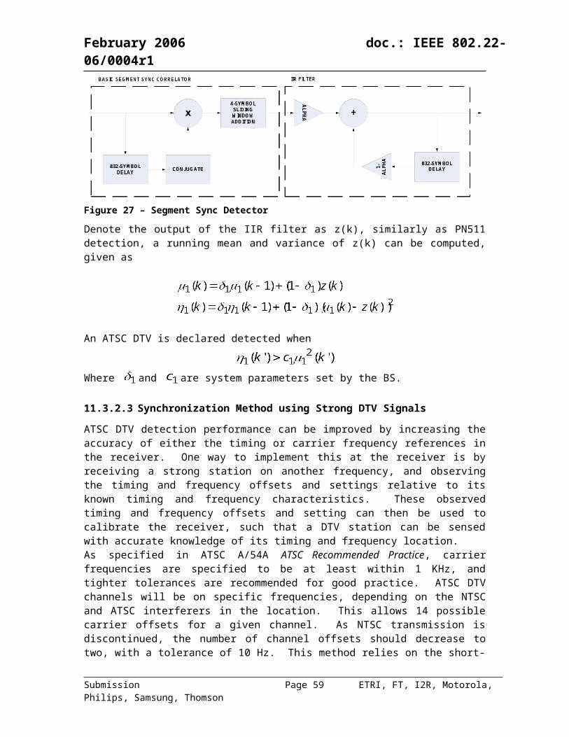
February 2006 doc.: IEEE 802.22-06/0004r1
Where is the SINR of user k, is the number of receive antennas of user k, and is the
identity matrix of size . Receiver filtering is performed by left multiplying the received
vector by or .
13.2.1.7 Signalling Requirements
A feedback channel for CPEs to report finite-rate quantized channel state information is required. Feedback does not have to be reported for every downlink frame, but it would be preferable in order to more accurately track the channel, at least for the users that are actually scheduled for downlink transmission.
13.2.1.8 Summary
The flowchart of operation of the proposed mode is shown in Figure 33.
Base station CPE
Quantized CSI and CQI feedback
Downlink sounding pilots and data
Downlink pilots
Channel estimation and computation of quantized CSI and CQI
Computation of transmit filters
Computation of receive filters and detection
Figure 33 – Timing of operations for CL-SDMA mode 1
13.2.2 CL-SDMA Mode 2: Using TDD with 3 or 4 Base Station Antennas and with 3 or 4 Antennas at the CPEs
When the WRAN operates in TDD mode, channel reciprocity can be relied upon to obtain estimates of the downlink channel from estimates of the uplink channel obtained at the base station. Calibration must be used to make these estimates reliable. The very slow fading nature of the WRAN channel makes these estimates accurate for several consecutive frames. Multiple CPE RF transmit chains must be available in order to estimate the MIMO channel at the base station. In other cases, this mode would not be applicable. However, when applicable, it offers very large throughputs.
Submission Page 59 ETRI, FT, I2R, Motorola, Philips, Samsung, Thomson
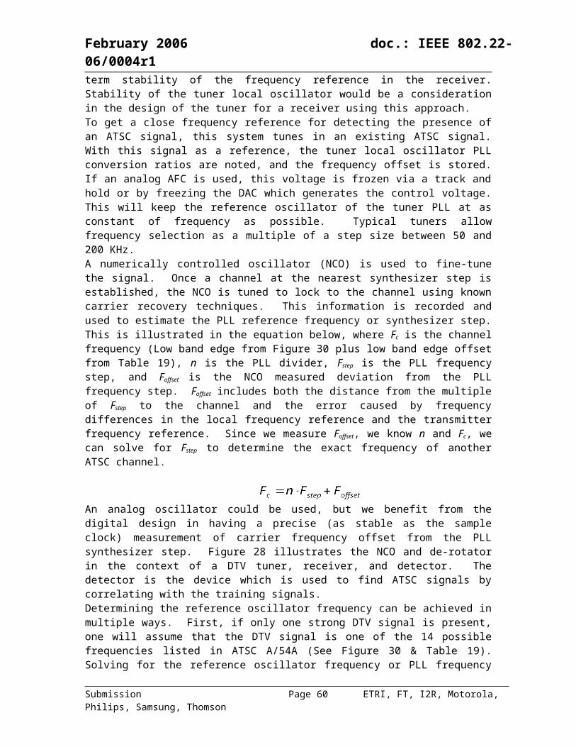
February 2006 doc.: IEEE 802.22-06/0004r1
13.2.2.1 Transmitter and Receiver Structure
Figure 34 shows the linear processing operations required at the transmitter and at the receivers of each active CPE on a given sub-carrier. Operations are carried in the frequency domain. The base station, as well as N CPEs, is required to be equipped with N antennas. This algorithm is applicable with any number of antennas at the N CPEs, however it is recommended to use N antennas at the CPEs. In particular with a single receive antenna at the CPEs, conventional downlink SDMA would provide better performance. The N CPEs are assumed to have been appropriately scheduled for the downlink for the proposed mode.
xk
x1
xN
W1*
x1 estimate
Wk*
xk estimate
WN*
xN estimate
Base station transmitter
downlinktransmission
M1
Mk
MN
1
2
k
N
CPE receiversFigure 34 – Transmitter and Receivers for CL-SDMA mode 2
13.2.2.2 Computation Phase at the Base Station
The base station has estimates of the downlink channel matrices of N users. The channel of user k is represented as . This estimate can represent the channel of a single sub-carrier, or of a group of adjacent sub-carriers. Then the base station performs the following computations:
Initialization: ( is the all-ones column vector)
for .
Repeat times:
Normalization:
Submission Page 60 ETRI, FT, I2R, Motorola, Philips, Samsung, Thomson
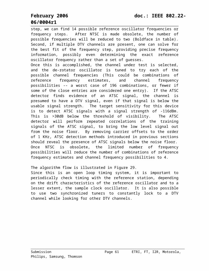
February 2006 doc.: IEEE 802.22-06/0004r1
for .
, the number of iterations, is a design parameter. Typically, it would be between 10 and 50, depending on N and on the channel conditions.
13.2.2.3 Downlink Data Transmission and Sounding
The process is the same as the CL-SDMA mode 1, with N base station transmit antennas and N users.
13.2.2.4 CPE Receiver Downlink Detection
The process is the same as the CL-SDMA mode 1, with N base station transmit antennas and N users.
13.2.2.5 Signalling Requirements
Uplink pilots coming from all N CPE antennas are required for the base station to estimate the uplink channel matrix. These pilots can be regular pilots in uplink data frames, or pilots designed specifically for the purpose of supporting this multiple antenna mode. Channel estimation does not need to be accomplished before every downlink frame in very slowly fading channels, but it would be preferable to more accurately track the channel, at least for the users that are actually scheduled for downlink transmission. On-demand uplink sounding schemes can be used to enhance the performance of this multiple antenna mode.
13.2.2.6 Other Requirements
In order to exploit channel reciprocity in TDD, the following requirements must be met: The time between uplink channel estimation and downlink transmission should be smaller
than the coherence time of the system The CPEs should be equipped with N RF transmit chains in order use all antennas for uplink
transmission The base station transmit antennas should be calibrated to compensate for propagation
differences in antenna RF chains for transmission and reception13.2.2.7 Summary
The flowchart of operation of the proposed mode is shown in Figure 35.
Submission Page 61 ETRI, FT, I2R, Motorola, Philips, Samsung, Thomson
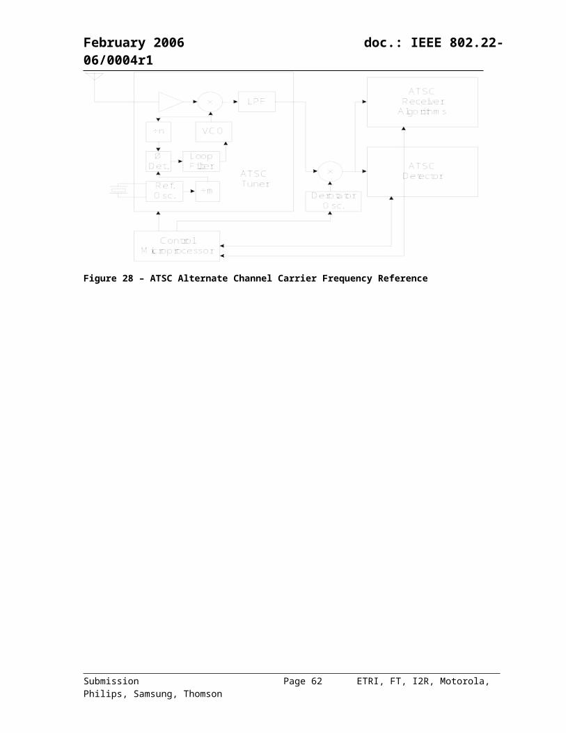
February 2006 doc.: IEEE 802.22-06/0004r1
Base station CPE
CQI feedback and uplink sounding pilots
Downlink sounding pilots and data
Downlink pilots
Channel estimation and computation of CQI
Computation of transmit filters
Computation of receive filters and detection
Figure 35 – Timing of operations for Closed-Loop CDMA mode 2
13.2.3 Downlink Pilot StructureThe downlink pilot structure in sub-channels with adjacent permutation sub-carriers is unchanged with respect to the default single antenna mode.
13.2.4 Other Signalling RequirementsSub-channel allocation information, modulation and rate formats must also be provided to the scheduled users in the control header of the downlink frame or super-frame, depending on the scheduling strategy.
13.3Adaptive Beamforming
Adaptive beamforming can mitigate the effect of co-channel interference (CCI) inherent to OFDMA systems and thereby can increase the frequency reuse factor close to unity. Since all CPE’s of WRAN systems are fixed at known locations, their directions-of-arrival (DOA’s) may easily be obtained and incorporated for adaptive beamforming without the need to be tracked. The large cell in WRAN networks also makes beamforming problem simple from 2D to 1D problem. So easy DOA estimation (if necessary) or beamforming using a simple array is available. In conjunction with the transmit diversity in the forward link and/or receive diversity in the reverse link, adaptive beamforming may significantly increase cell radius, as required for WRAN systems. The adaptive beamforming also significantly reduces multi-path delay spread, which enhances system efficiency. As shown in Figure 36, the adaptive array system steers the main beam to the direction of a desired signal, while steering nulls to the directions of undesired interference signals.
Submission Page 62 ETRI, FT, I2R, Motorola, Philips, Samsung, Thomson
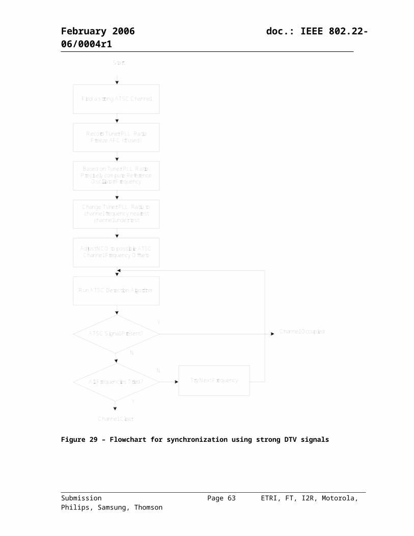
February 2006 doc.: IEEE 802.22-06/0004r1
adaptive arrayfixed-beam
Figure 36 – Adaptive Array Vs. Fixed-Beam Array
13.4Full Diversity Full Rate (FDFR) Scheme
While space-time coding tries to enhance the link reliability by capturing spatial diversity, multiplexing schemes like BLAST pump more streams of data into MIMO channels for increased throughput. In FDFR scheme, the two opportunities in MIMO channels, diversity and multiplexing are jointly attained at the same time in a scheme. The original FDFR scheme [5] is designed for square matrices and in need of complex processing both at the transmitter and at the receiver sides. The proposal provides a scheme that facilitates successive interference cancellation scheme with ML or sphere decoding for the pre-coder decoding. The scheme leaves the tail edge sides of the transmission matrices with zero symbols, thus loses some of the rate from the full rate pledged, but still guarantees the full diversity with almost full rate depending on the block size. The transmitter side operation is shown in the figure below, where we show a transmission matrix for three antennas and block size 7 is used.
Figure 37 – Full Diversity Full Rate (FDFR) scheme and an example transmission matrix for a 3-antenna system using a block size of 7
The matrix given above satisfies full rank condition for any pair of error cases due to the pre-coder and diagonal positioning of pre-coded vectors. 6 zero-positions corresponding to rate loss
Submission Page 63 ETRI, FT, I2R, Motorola, Philips, Samsung, Thomson
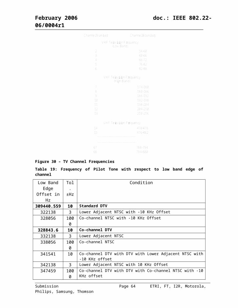
February 2006 doc.: IEEE 802.22-06/0004r1
are shown in this 3 by 7 example. The ratio of zeroed positions compared to total transmission symbols is reduced if the block size gets longer. It is the structure of the matrix given above that enables successive interference cancellation with ML or sphere decoder, where interference from the previous vectors is cancelled while that from the later vectors is suppressed.
13.5Additional Transmit Beamforming Modes
13.5.1 Simple Downlink Transmit Beamforming
The block diagram of the beamforming transmitter at the BS using a single beam with transmit antennas is illustrated in Figure 38. Transmit beamforming is implemented in the frequency domain. As each sub-channel may be assigned exclusively to a user, beamforming is done at the sub-channel level, since each of the users usually has a different channel response. The modulated data symbols of the l-th user is first weighted by the beamforming weights,
, where is the coefficient associated with the n-th transmit antenna. Therefore, the transmitted signal of the l-th user over the k-th sub-carrier via the n-th transmit antenna is
where is the signal at the k-th sub-carrier before beamforming. The transmission is steered in the direction with the highest gain. Physically, this beamformer points the main beam’s direction to the desired user, while the other directions are ignored. The beamforming vector is equivalent to the principle eigenvector of the downlink covariance matrix , and the transmission channel is therefore the eigen-channel with the strongest gain. Assuming TDD transmission, the downlink covariance matrix may be estimated from the uplink since the channel is reciprocal. In general, downlink channel covariance matrix of the l-th user is
where is the downlink covariance matrix of the i-th beam, is the associated average power is its DOA. The i-th antenna steering vector is defined as
for a uniform linear array with antenna spacing d, and is the wavelength of the carrier or center frequency.Simple transmit beamforming using a single beam is most suitable for channels with overall covariance matrices of rank 1. This scenario arises when there is a single beam with dominant average power. In this case, the suppression of the other directions does not significantly affect the performance of the system.
Submission Page 64 ETRI, FT, I2R, Motorola, Philips, Samsung, Thomson

February 2006 doc.: IEEE 802.22-06/0004r1
Figure 38 – Downlink transmitter block diagram for simple frequency domain beamforming with NT antennas
Downlink beamforming can also be done in the time domain. Figure 39 shows the downlink transmitter block diagram for simple time domain beamforming. Each user will have an individual OFDM modulator. Sub-carriers unused by a particular user are zero padded. After OFDM modulation, the cyclic prefix is added and this is followed by windowing and pulse shaping. The transmitted signals are then weighted by their respective beamforming weights, summed and transmitted. Note that the frequency and time domain implementations are essentially equivalent.
Figure 39 – Downlink transmitter block diagram for simple time domain beamforming with NT antennas
Submission Page 65 ETRI, FT, I2R, Motorola, Philips, Samsung, Thomson
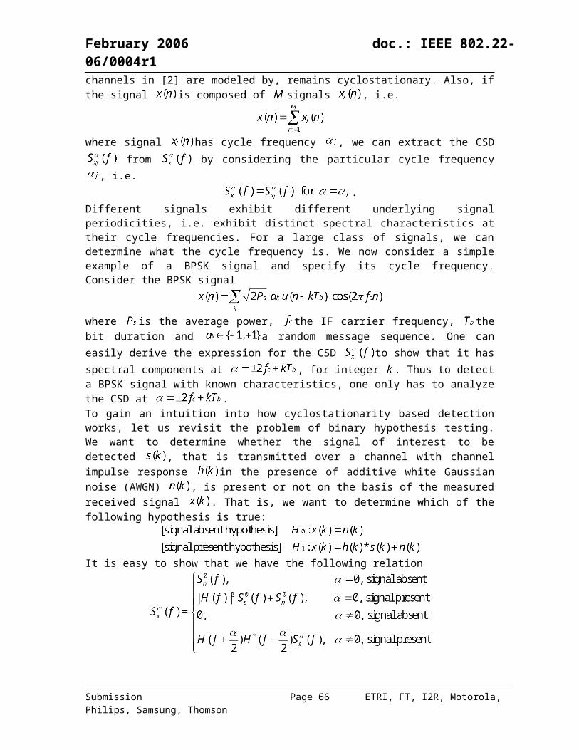
February 2006 doc.: IEEE 802.22-06/0004r1
13.5.2 Downlink Transmit Beamforming with Diversity/Spatial MultiplexingFor users’ channels with covariance matrix greater than rank 1, more than one beamformer may be used together with transmit diversity techniques to improve performance. We will consider an example with 2 beamformers per user, though the system may be generalized to a number of beamformers up to the rank of the channel covariance matrix. Figure 40 and Figure 41 show the transmitter block diagrams for the downlink of a system with transmit antennas using frequency and time domain beamforming respectively. The transmitter combines beamforming and CDD (see Annex A.1). For each user, two equivalent streams of the transmitted data symbols are generated. To achieve diversity advantage, the data symbols are mapped from channel encoded data bits. Like the simple case with one beamformer per user, each sub-carrier of the first data stream is simply weighted by its first beamformer. For the second stream, each sub-carrier is first phase shifted appropriately before weighting by the second beamformer. CDD may be implemented by performing a cyclic shift of Tl on the time domain data block before adding the cyclic prefix, or it may be done in the frequency domain by
applying a phase shifter , on the k-th sub-carrier. The sub-carrier outputs of the
two beamformers are summed together before OFDMA modulation. For , the transmitted signal of the l-th user over the k-th subcarrier via the n-th transmit antenna is
,
where and are the coefficients of the first and second beamformers of user l respectively.The beamforming weights are equivalent to two principle eigenvectors of the channel covariance matrix . By using beamforming two uncorrelated transmission channels are created. Performance improvement is achieved due to application of CDD.
Submission Page 66 ETRI, FT, I2R, Motorola, Philips, Samsung, Thomson
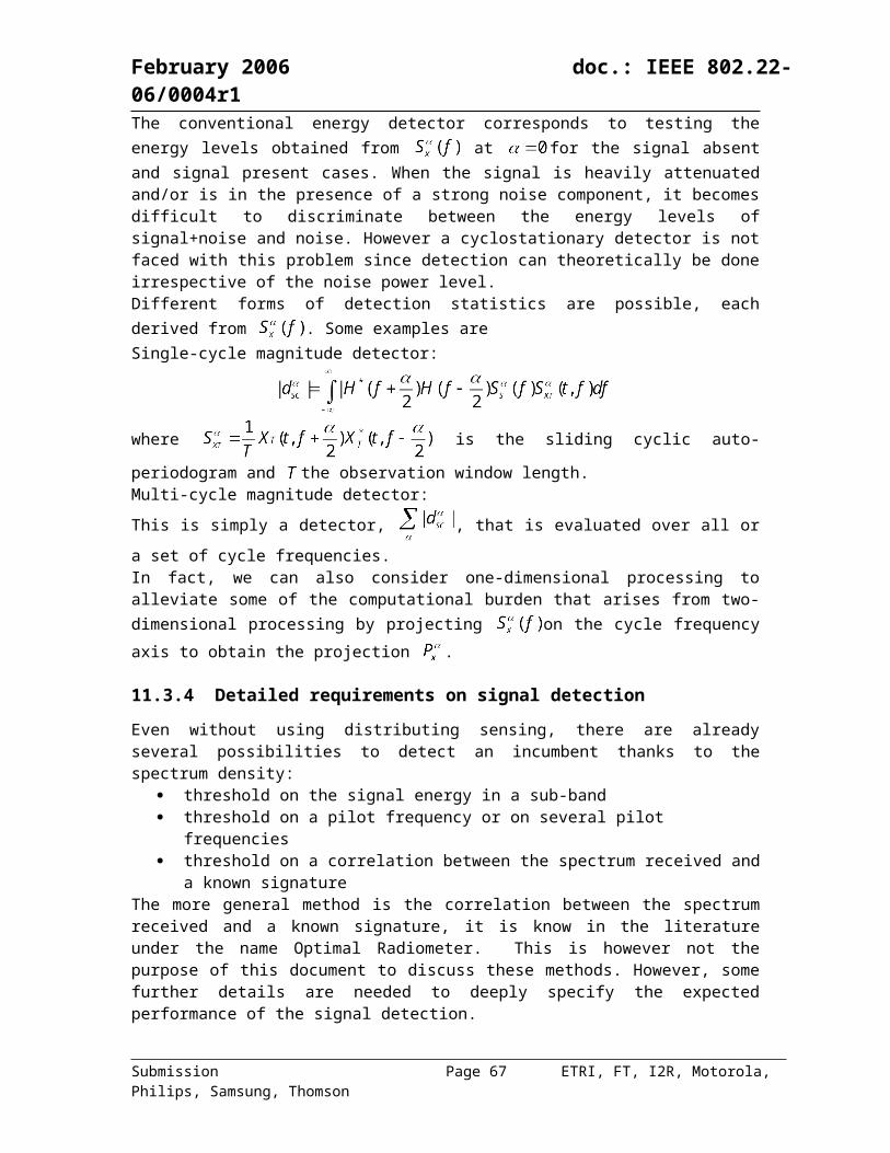
February 2006 doc.: IEEE 802.22-06/0004r1
Figure 40 – Downlink transmitter block diagram for combined frequency domain beamforming and CDD with NT antennas
Figure 41 – Downlink transmitter block diagram for combined time domain beamforming and CDD with NT antennas
Performance gain with respect to throughput is also achievable by combining beamforming and spatial multiplexing. We consider the case with 2 beamformers per user. Since each beamformer
Submission Page 67 ETRI, FT, I2R, Motorola, Philips, Samsung, Thomson
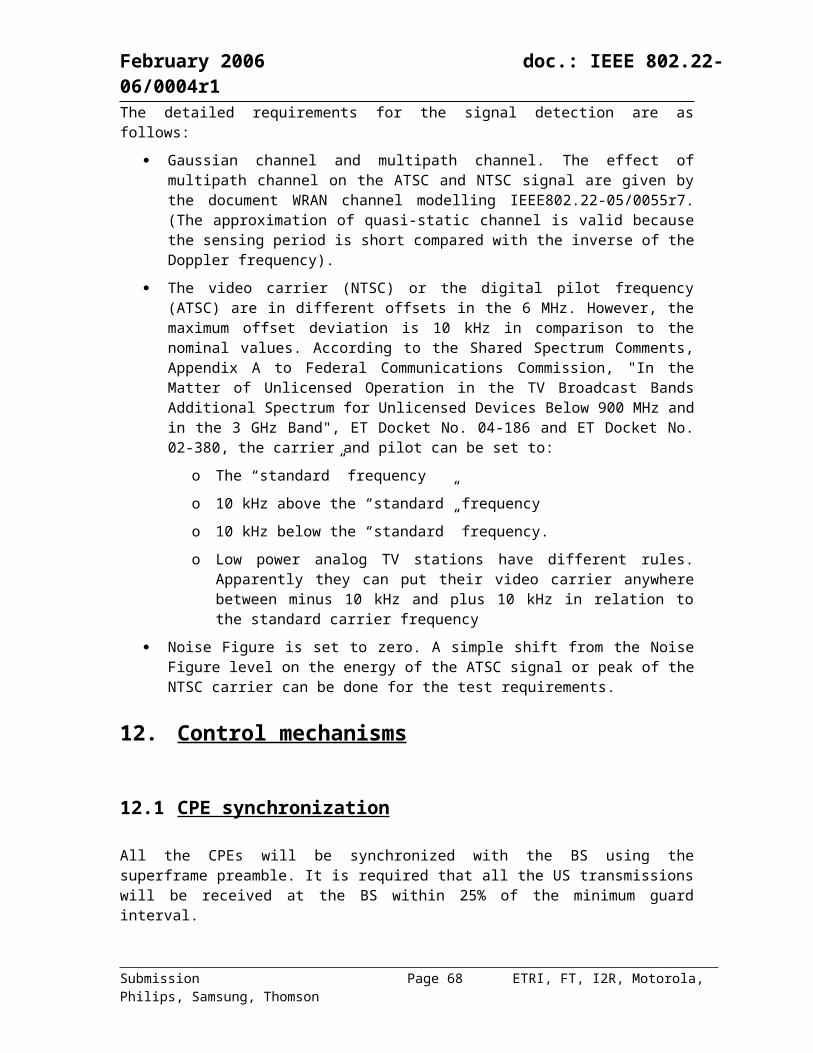
February 2006 doc.: IEEE 802.22-06/0004r1
creates an uncorrelated transmission channel, the data symbols of each user may be multiplexed onto each channel and transmitted. Therefore, the number of data symbols transmitted over the allocated sub-carriers per user is effectively doubled. Figure 42 and Figure 43 illustrate the transmitter block diagrams for frequency and time domain combined beamforming and spatial multiplexing respectively.
Figure 42 – Downlink transmitter block diagram for combined frequency domain beamforming and spatial multiplexing with NT antennas
Submission Page 68 ETRI, FT, I2R, Motorola, Philips, Samsung, Thomson
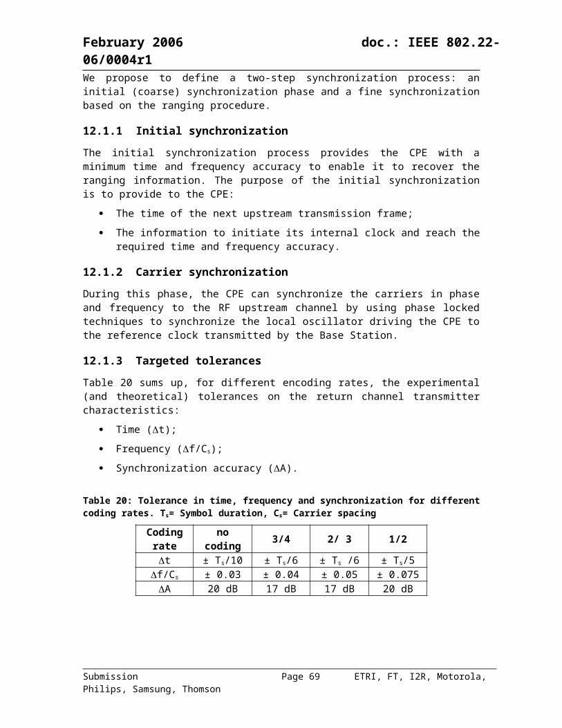
February 2006 doc.: IEEE 802.22-06/0004r1
Figure 43 – Downlink transmitter block diagram for combined time domain beamforming and spatial multiplexing with NT antennas
13.5.3 Downlink Transmit Beamforming with Diversity/Spatial Multiplexing and Channel Delay Management
There are instances where the overall channel delay exceeds the cyclic prefix period. This leads to inter-block interference (IBI). However, we exploit the fact that different DOAs may be associated with different delays. Using beamforming, we may combined beamforming, diversity/spatial multiplexing and channel delay management. Since the different beams are isolated from one another, they may be pre-aligned in time before transmission, so that the overall delay of the transmission is reduced.Consider the case where there are 2 distinct DOAs, and , for l-th user’s channel in the downlink. Associated with each of DOAs is a cluster path, with intra-cluster delay δ l. Delays τ1,l
and τ2,l, corresponds to the and respectively. If the cluster only contains a single path, then δl = 0. When exceeds the cyclic prefix duration , inter-block interference is present. Beamformers may be designed to direct two beams, each to one of the clusters. A delay is applied to each OFDMA block to be transmitted via each beam. D 1,l and D2,l are the delays associated with the first and second beam respectively. Therefore, the resulting nominal delay for direction 1 is , and for direction 2 is . The magnitude of the relatively delay of the beamformed channel is now . Hence, if we choose D1,1 and D2,l such that , then the CP duration becomes sufficient in preventing IBI. Channel delay management may be used with CDD (see Annex A.1) and spatial multiplexing for enhanced performance. Figure 44 and Figure 45 illustrate the transmitter block diagram of combined time domain beamforming and CDD/spatial multiplexing with channel delay management.
Submission Page 69 ETRI, FT, I2R, Motorola, Philips, Samsung, Thomson

February 2006 doc.: IEEE 802.22-06/0004r1
For the l-th, the beamformer coefficients may be computed using the directional channel covariance matrices and associated with DOAs and respectively. The first beamformer is equivalent to the principle eigenvector of the matrix pencil principle eigenvector of the matrix pencil , which may be obtained using the generalized eigen decomposition. Likewise, the second beamformer is equal to the principle eigenvector of the matrix pencil .
Figure 44 – Downlink transmitter block diagram for combined time domain beamforming and CDD with channel delay management using NT antennas
Submission Page 70 ETRI, FT, I2R, Motorola, Philips, Samsung, Thomson

February 2006 doc.: IEEE 802.22-06/0004r1
Figure 45 – Downlink transmitter block diagram for combined time domain beamforming and spatial multiplexing with channel delay management using NT antennas
13.6Virtual Multiple Antenna System
Although some CPEs may only each have a single transmit antenna, a virtual multiple transmit antenna system may be implement at the CPEs to increase the spectral efficiency of the system. As an example, we consider a system with 2 transmitting CPEs and 1 BS. As shown in Figure 46, CPE1 transmits its signal through CPE1 antenna, whereas CPE2 transmits through CPE2 antenna. Hence, a virtual multiple antenna transmitter is formed and it is analogous to a transmitter with two antennas. From the BS point of view, it is receiving two spatially multiplexed transmissions. As long as the BS has two or more antennas, de-multiplexing and detection of the data is possible. In such a case, CPE1 and CPE2 can share the same frequency resource at the same time.
Submission Page 71 ETRI, FT, I2R, Motorola, Philips, Samsung, Thomson
February 2006 doc.: IEEE 802.22-06/0004r1
Figure 46 – Virtual multiple antenna system for uplink transmission
Annex A (Informative) – Recommended Practices and Procedures
A.1 Cyclic Delay Diversity (CDD) Transmission Cyclic delay diversity (CDD) transmission may be implemented at the CPE equipped with multiple antennas. Figure 47 shows the block diagram of CDD applied to a system with two transmit antennas. For diversity gain, the data symbols must be encoded, usually using FEC and interleaving, across the transmission bandwidth. The outputs are then OFDMA modulated. As an example, we let the OFDMA size be N = 8, and the cyclic delay T = 2. The transmitted OFDMA symbol via antenna 1 is
x1 = [s(0), s(1), s(2), s(3), s(4), s(5), s(6), s(7)] ,
and the cyclic delayed version of x1,
x2 = [s(6), s(7), (0), s(1), s(2), s(3), s(4), s(5)],
will be sent out through antenna 2.Referring to Figure 48, the channel responses with respect to antenna 1 and 2 are denoted as
and respectively, where L is the number of channel delay taps, and their respective frequency responses are and
.With CDD, the frequency responses of the composite channel observed by the receive antenna is given by
Submission Page 72 ETRI, FT, I2R, Motorola, Philips, Samsung, Thomson
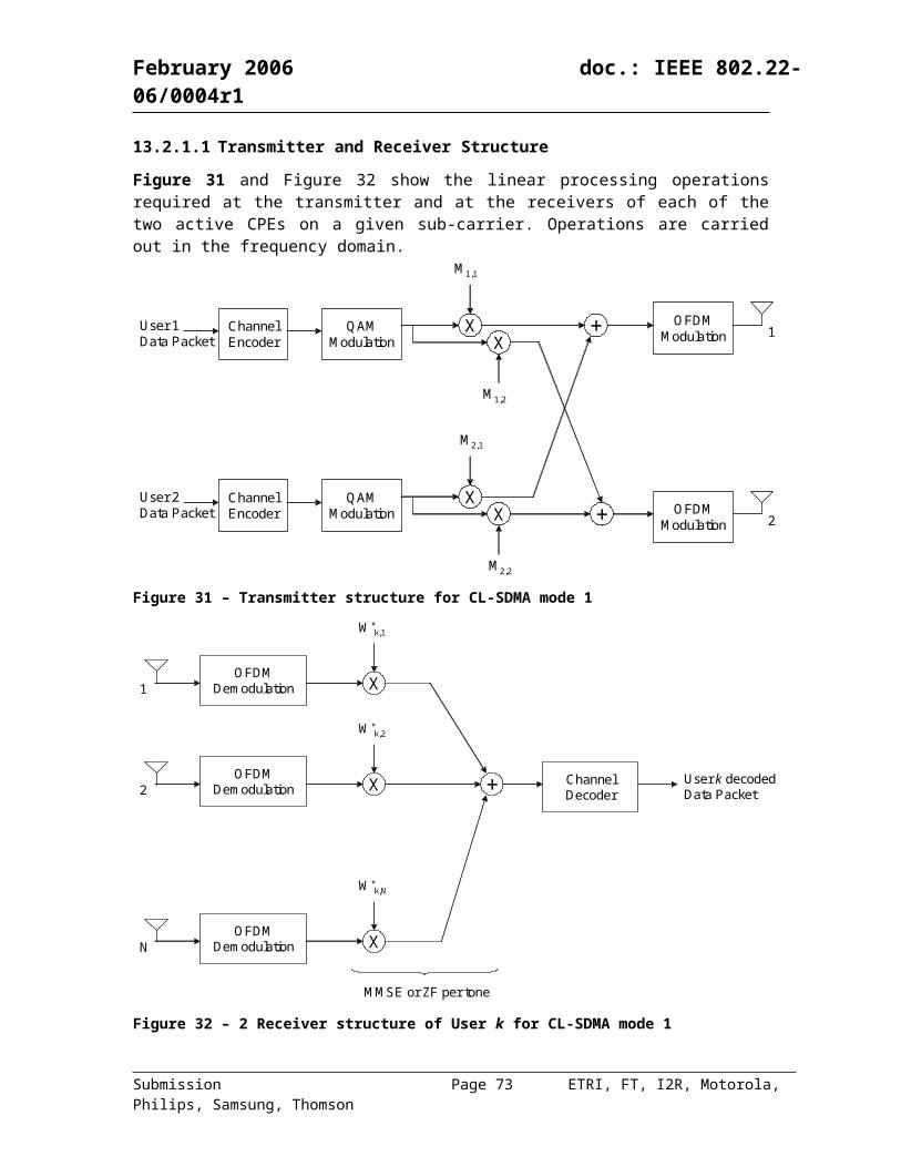
February 2006 doc.: IEEE 802.22-06/0004r1
where k is the sub-carrier index, and T is the cyclic delay in symbols. It can be shown that higher frequency diversity is achievable through CDD. Typical cyclic shift factor is in the range 0 < T < N, for diversity gain. An example of the composite virtual channel response with 2 transmit antennas is illustrated in Figure 49, where the original channel responses associated with each antenna is L = 2, and cyclic delay is T = 2. By applying CDD, the composite channel response becomes h1(0), h1(1), h2(0), h2(1), and the number of channel taps in the virtual channel increases to 4. The delay diversity may be exploited to enhance the performance of the system by employing cross band coding. Although the number of delay taps of the composite virtual channel is 4, the physical channel delays associated with both antennas remain unchanged at 2. Unlike conventional delay diversity, the CDD does not increase the physical delay of the composite channel. Therefore, the minimum required CP length remains unchanged at 1 symbol interval.In the above example, the frequency domain representation of the data symbol on the kth sub-
carrier transmitted through antennas 1 and 2 are and , respectively.
Therefore, CDD can be implemented by phase shifting kth data symbol by prior to
OFDMA modulation for the second antenna. This approach, which is frequency domain implementation of CDD may be advantageous in the downlink as different groups of sub-carriers (sub-channels) would generally have different channel responses, and the cyclic shifts requirements for the different channels may also differ. If CDD in time domain is employed in this case, each sub-channel, in general, would require an additional OFDMA modulator and cyclic shifter, which could increase the complexity dramatically. Hence, by deploying frequency domain CDD, the different cyclic delay requirements are individually met, without a significant increase in complexity.
Figure 47 – Block diagram of CDD with 2 transmit antennas
Submission Page 73 ETRI, FT, I2R, Motorola, Philips, Samsung, Thomson
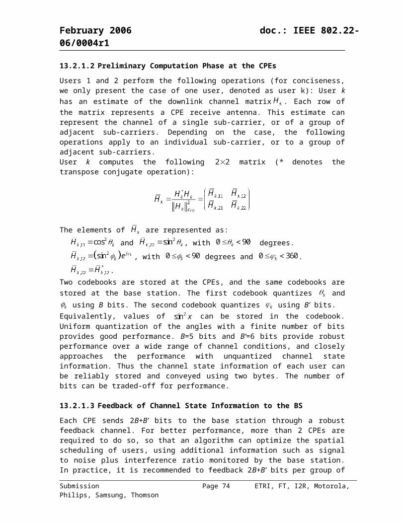
February 2006 doc.: IEEE 802.22-06/0004r1
Figure 48 – Transmission model for CDD
Figure 49 – Equivalence of the composite channel
A.2 Sectorization Sectorization is a simple and effective method to support increased number of users within a coverage area. Figure 50 illustrates an example of dividing one cell into three sectors, each covered by one sector antenna. It is expected that a capacity gain of three can be achieved as compared to the case without using sectorization.
Submission Page 74 ETRI, FT, I2R, Motorola, Philips, Samsung, Thomson
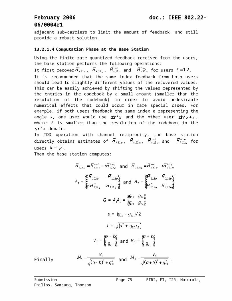
February 2006 doc.: IEEE 802.22-06/0004r1
Figure 50 – An example of sectorization by dividing one cell into three sectors
A.2.1 Scrambling code design In order to distinguish different sectors, it is proposed that each sector is allocated with a different set of scrambling codes. Figure 51 shows the transmitter structure for BS with three sectors.The generation of scrambling codes for each sector is illustrated in Figure 52. Take sector 1 as the reference sector. We can randomly generate the codes for the first OFDMA symbol, and choose the scrambling codes for symbols 2, 3, … as the cyclically delayed versions (each delayed by one sample) of scrambling codes of symbol 1. For sectors 2 and 3, the scrambling codes are generated as those of sector 1 scaled by the phase shifters. For example, if the scrambling codes for sector 1 are given by
The scrambling codes for sectors 2 are given by
The scrambling codes for sector 3 are
Submission Page 75 ETRI, FT, I2R, Motorola, Philips, Samsung, Thomson
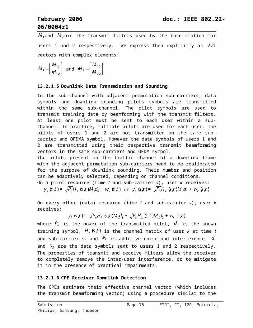
February 2006 doc.: IEEE 802.22-06/0004r1
The parameters and can be chosen as and , where is the maximum excess delay of the propagation delay of the channel.
Figure 51 – BS transmitter with three sectors each allocated allocated with a different set of scrambling codes
Submission Page 76 ETRI, FT, I2R, Motorola, Philips, Samsung, Thomson
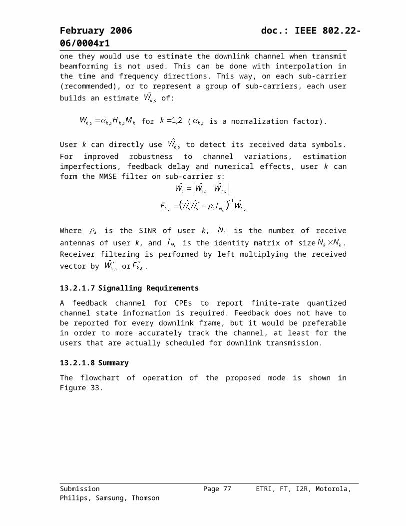
February 2006 doc.: IEEE 802.22-06/0004r1
Figure 52 – Scrambling code generation for the three sectors within the same cell
A.2.2 Inter-sector diversity Suppose the sector antennas have a 3-dB beamwidth of 120o, with reference to Figure 53, user #3 located in the sector edge may receive signals from both antennas simultaneously. To minimize the interference effect and to provide increased throughput for sector edge users, the proposal suggests that two neighbouring sectors serve the sector edge users using the same sub-channel simultaneously. This is called inter-sector diversity.
Figure 53 – Inter-sector diversity
The block diagram of BS transmitter with inter-sector diversity is illustrated in Figure 54. The same set of pilot symbols are transmitted to all sectors, and the sector edge users can be transmitted through two neighbouring sectors. However, again, each sector is allocated with a different set of scrambling codes.The scrambling codes are generated as follows. Take sector 1 as the reference sector. We can randomly generate the codes for the first OFDMA symbol, and choose the scrambling codes for symbols 2, 3, … as the cyclically delayed versions of scrambling codes of symbol 1. To support transmit diversity for pilot and sector edge users, for sectors 2 and 3, the scrambling codes are
Submission Page 77 ETRI, FT, I2R, Motorola, Philips, Samsung, Thomson
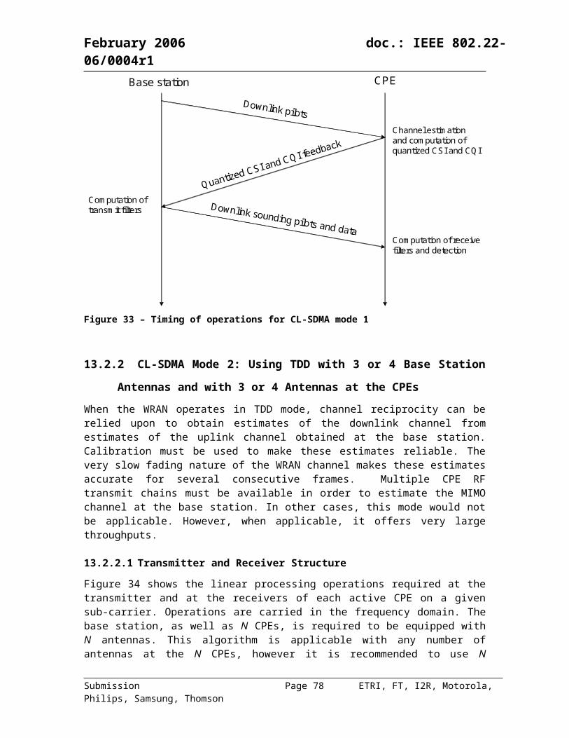
February 2006 doc.: IEEE 802.22-06/0004r1
generated as those of sector 1 scaled by the phase shifters, which are related to the time domain cyclic shifts. Suppose user k is allocated with the sub-channel with sub-carrier index set , and the cyclic shift for user k is . The frequency domain implementation modulates the
frequency signal of user k for the second antenna with a phase shifter , where
. If time division pilot pattern is used as shown in Figure 55, the first OFDMA symbol is chosen as the pilot symbol for all sectors. For sector edge users, each modulated symbol is transmitted over the same sub-carrier of the two serving sectors.Suppose user A is located in the edge between sectors 1 & 2, user B in the edge between sectors 2 & 3, and C in the edge between sectors 1 & 3. We then allocate the first sub-channel of sectors 1 & 2 to user A, the 5th sub-channel of sectors 1 & 3 to user B, and the 8 th sub-channel of sectors 1 & 3 to user C. The remaining sub-channels of each sector are then allocated to the users within that sector. The scattered pilot pattern is shown in Figure 56, where the edge users again are allocated with the same sub-channel from two neighbouring sectors.
Figure 54 – BS transmitter with inter-sector diversity
Submission Page 78 ETRI, FT, I2R, Motorola, Philips, Samsung, Thomson
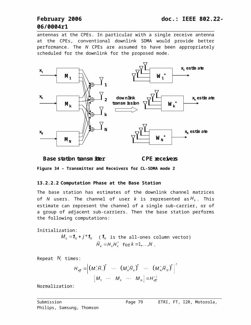
February 2006 doc.: IEEE 802.22-06/0004r1
Figure 55 – Time division pilot patterns for three sectors within the same cell
Figure 56 – Scattered pilot patterns for three sectors within the same cell
A.3 Sensing Antenna Design
As part of interference avoidance, the WRAN device is required to detect television signals produced by field strengths as low as 21 dBuV/m over a 6 MHz television channel. Since the licensed transmitter may be at any location relative to the WRAN unit, such sensing must be made for a 360-degree circle. Such an antenna for horizontal polarization is very difficult to achieve and can only be done over a few 6 MHz television channels. In particular, two horizontal
Submission Page 79 ETRI, FT, I2R, Motorola, Philips, Samsung, Thomson
February 2006 doc.: IEEE 802.22-06/0004r1
dipoles can be placed orthogonal to each other and the outputs added. This would, at first examination, achieve an approximate omni-directional pattern. However, at the 3 dB points of each pattern, the signals from each antenna are equal, but of undetermined phase. This can result in an out of phase addition that produces a deep null at one or more of those 4 points. It is possible to carefully adjust the phasing to minimize that null for a narrow band of frequencies such as one or two 6 MHz television channels. This can be done for television broadcast antennas but requires considerable added complexity. However, this type of control cannot be achieved over a wide band of frequencies such as the complete UHF television band.
This proposal is to provide two or more antennas with overlapping patterns. The antennas are to be alternatively switched electronically to a common measurement apparatus. If any of the antennas produce an indicated field strength above the limit, then the frequency is in use and must be avoided. For example, two orthogonal dipoles could be used. Each dipole produces a figure 8 pattern with each lobe having a 3 dB beamwidth of approximately 90 degrees. By switching and measuring each antenna separately, a full 360-degree circle is covered. The gain of a dipole is 2.12dBi. At the 3 dB points, the gain would be -0.88 dBi which is close to, but not within the prescribed limit of 0 dBi gain. If this is not acceptable, 3 dipoles could be arranged with uniform radial spacing.
If the signal from such a dipole arrangement is not sufficiently high enough for the detection means used, then each of the dipoles may be augmented by additional dipoles stacked vertically. For example, a two by two dipole arrangement would give an additional 3 dB gain in output signal. It is also possible to make an arrangement of 4 antennas spaced 90 degrees with a unidirectional pattern: an example would be an arrangement of 4 corner reflectors. Such antennas have approximately 90 degree 3 dB beamwidths and a gain of 8 dBi.Although it may require some time to switch to each antenna and make the multiple measurements, this time may be compensated by producing a higher signal level that is more quickly detected in the presence of noise.
A.4 Antenna Installation Method
The Wireless Regional Area Network (WRAN) system proposed by IEEE 802.22 requires mitigating interference to incumbent television service. One method is to operate the two services in orthogonal antenna polarizations. In the USA, television is generally transmitted with horizontal polarization. A proposed system for an unlicensed WRAN would share those frequencies. To minimize interference, the WRAN should transmit using vertical polarization. An exemplary desired cross polarization isolation is given as 14 dB.
The isolation achieved, assuming a properly designed and manufactured antenna, is proportional to the cosine of the angle between the transmitting and receiving antennas. Thus, if the antennas are 90 degrees to each other, the isolation is infinite. However, if the angle is 78.5 degrees, the isolation is 14 dB. If we were to assume equal error on the transmit and receive antennas, this would imply that the transmit antenna must be installed with an error of 5.5 degrees or less. The proposed service states that the equipment can be user installed. Thus, no skill can be assumed with respect to proper alignment.
A solution to this problem is to provide a level sensitive switch in the antenna structure that would be in one state when the antenna is aligned within a specific tolerance and in another state when positioned improperly. The state resulting from improper positioning could be used to prevent transmitter operation, reduce the transmitter power to a lower level or to signal to a service provider that the antenna was misaligned and required professional service.
Submission Page 80 ETRI, FT, I2R, Motorola, Philips, Samsung, Thomson

February 2006 doc.: IEEE 802.22-06/0004r1
As a specific example, the switch could be made as a conductive pendulum inside a conductive tube. By design of the length of the pendulum and the diameter of the tube, the degrees of misalignment before the pendulum and tube make contact can be controlled to any desired value. This contact can close a circuit to indicate misalignment and control transmitter operation as above.
To MonitoringCircuitry
InsulatingSupport
ConductiveWeight
ConductiveTube
Figure 57 – Level sensitive switch
In Figure 57, the switch is incorporated in a metal tube that could be part of the mounting past for the antenna structure. In the cut away drawing, a small flexible wire is suspended from an insulating support and a second wire is connected to an external monitoring circuit. A conductive weight is connected to the other end of the flexible wire so that the wire and weight will rotate freely to be vertical under the influence of gravity. As shown in Figure 57, the tube is vertical. The weight does not touch the sides of the tube and correct alignment is indicated by presenting an open circuit to the monitoring circuitry.
To MonitoringCircuitry
Figure 58 – Antenna misalignment indication
In Figure 58, the tube has suffered a rotation and is no longer vertically oriented. The flexible wire and weight assembly do touch the side of the tube. This presents a closed circuit which can be detected by the monitoring circuitry.
Submission Page 81 ETRI, FT, I2R, Motorola, Philips, Samsung, Thomson