Embed Size (px)
Citation preview
Do Transfer Taxes Reduce Intergenerational Transfers?∗
Tullio Jappelli†
University of Naples Federico II, CSEF and CEPR
Mario Padula‡
University Ca’ Foscari of Venice, CSEF and CEPR
Giovanni Pica§
University of Salerno and CSEF
November 8, 2012
Abstract
We estimate the effect of taxes on intergenerational transfers exploiting a sequence ofItalian reforms culminating with the abolishment of transfer taxes. We use the 1993-2006Survey of Household Income and Wealth, which has data on real estate transfers receivedand information on potential donors as well as recipients. Differences-in-differences es-timates indicate that the abolition of transfer taxes increased the probability that high-wealth donors make a transfer by 2 percentage points and square meters transferred by9.3 meters relative to poorer donors.
JEL Classification: H24, E21.Keywords : Transfer Taxes, Intergenerational Transfers. Intergenerational Mobility
∗We thank Andrea Ichino, Luigi Pistaferri and seminar participants at the University of Naples Federico IIand University “Ca Foscari” of Venice for comments, and the Italian Ministry for Universities and Research(MIUR) for financial support. The usual disclaimer applies. Part of the project was carried out while MarioPadula was a Fulbright Scholar at the Department of Economics of Stanford University.†Department of Economics, University of Naples Federico II, Via Cinzia, Monte S. Angelo, 80126, Napoli,
Italy. E-mail: [email protected].‡Department of Economics, University of Venice, Cannaregio 873, 30121, Venice, Italy. E-mail:
[email protected].§Department of Economics, University of Salerno, Via Ponte Don Melillo, 84084, Fisciano (SA), Italy. E-mail:
1
1 Introduction
Most developed countries, including the U.S. and the vast majority of European countries, tax
intergenerational transfers. Two main taxes are levied on bequests and gifts: the estate tax,
which is levied on the total estate of the donor, regardless of the characteristics and number
of recipients, and the inheritance tax, which is levied on the share of transfers received by
recipients. Even though in OECD countries the yield of transfer taxes hardly exceeds 1 percent
of total government revenues, taxing intergenerational transfers is the subject of intense quarrels
both in the U.S. and Europe because of the potential effects on capital accumulation and
intergenerational wealth mobility (Gale & Slemrod, 2001). However, the policy debate lacks
reliable estimates of the effect of transfer taxes on the propensity to bequeath, and therefore
fiscal revenues, wealth transmission and intergenerational mobility.
Few empirical studies have attempted to estimate the tax elasticity of bequests. To our
knowledge all focus on the U.S., see Kopczuk (2009) for a recent survey. Estimating the
effect of taxes on bequests is difficult because suitable data on both donors and recipients
are hard to find. Some studies use information provided by fiscal revenues, while others rely
on microeconomic data on wealth accumulation. Time series studies encounter the problem
that changes in fiscal revenues and tax rates tend to be correlated with other variables. In
cross-sectional studies it is hard to disentangle the effect of taxes on bequests from potential
confounding effects, including tax avoidance and unobservable preference traits (for instance,
preference for thrift or work).
In this paper we estimate the effect of transfer taxes on bequests using Italian survey
data and exploiting the variability in tax rates induced by a sequence of reforms that reduced
substantially estate, inheritance and gift taxes in 1999 and ultimately abolished them in 2001.
The cancellation of taxes did not affect all households equally, because the reform had no
impact on relatively poor donors who were already exempt from estate taxation prior to the
reforms. This allows us to cast our analysis in a quasi-experimental framework and to identify
the effect of the reform comparing the change in transfers given by individuals affected by the
reform with the change in transfers given by individuals unaffected by the tax change. Our
analysis is particularly valuable because we rely on a large change in estate tax policy for
identification. Indeed, recent research by Chetty (2009) makes a strong case that behavioral
elasticities estimated in response to subtle tax changes are likely to underestimate responses to
2
taxes, because the utility loss from ignoring small changes is often negligible and the cost of
understanding tax reforms may be large.
We use the 1993-2006 Bank of Italy Survey of Household Income and Wealth (SHIW),
which is representative of the Italian population. The survey includes information on the
number and size (in square meters) of real estates received at any time as inheritance and,
for respondents and spouses, data on parents’ education and occupation. Thus we can merge
information on donors and recipients to study if the cancellation of estate taxation has affected
intergenerational transfers. The availability of data on donors and recipients is crucial in this
context, because the decision to transfer and how much to transfer is affected by both donors’
as well as recipients’ characteristics.
The richness of the data and the specific characteristics of the tax reform provide three
advantages for spotlighting the effect of transfer taxes on the intergenerational transmission of
wealth. First, the quasi-experimental setting allows us to estimate the causal impact of the
cancellation of transfer taxation on bequests. Second, we analyze microeconomic data with
information on both potential donors and recipients. Finally, our sample is representative of
the Italian population at large. With the notable exception of Holtz-Eakin and Marples (2001),
previous literature has relied on administrative data, and therefore focuses on a selected group
of rich taxpayers.
We find that the relation between transfer taxes and the propensity to transfer real assets
is negative and statistically significant. Difference-in-difference estimates suggest that after the
reform the probability of observing real estate transfers increases by 2 percentage points. The
average effect of taxes on square meters transferred is also positive and statistically different
from zero. After the reform transfers increase by 9.3 square meters. Under the assumption that
square meters transferred are proportional to property values, this suggests a tax elasticity of
around -0.1 percent, a number that should be used with care when predicting the effect of
other tax reforms.1 Results from quantile regressions show that the effect of the reform is
stronger in the upper tail of the distribution of transfers. We cannot rule out misclassification
in the treatment and control groups, but we are able to establish that in the presence of
1Kopczuk and Slemrod (2001) find an elasticity of -0.16 percent of reported transfers with respect to taxes forthose who die with a will. They also find that the effect of taxes is stronger for those who die at more advancedages. Their results are stronger when they use aggregate data and more fragile in their pooled cross-sectionalanalysis. Joulfaian (2006) uses federal government estate tax collections data and finds an elasticity of justbelow -0.1 percent.
3
misclassification the true effect of the reform is likely to be underestimated.
Our estimates share with existing studies also some drawbacks, chiefly that the reform might
have had not only a genuine tax effect, but also a portfolio effect. In particular, since we have
data only on transfers in the form of real estate (not on total transfers), we cannot rule out
that after the reform donors are more willing to transfer wealth in the form of real estate,
rather than in other forms, such as liquid assets. To tackle the issue, we present evidence on
cohort-specific profiles of transfer behavior and data on total transfers that suggest that a tax
effect is more likely to explain the empirical results. The remaining of the paper is organized as
follows. Section 2 reviews the theoretical and empirical literature on bequest taxation. Section
3 describes the Italian tax reform and Section 4 the data. The empirical strategy is discussed
in Section 5, and the empirical results are presented in Section 6. Section 7 summarizes our
main findings.
2 The effect of taxes on intergenerational transfers
Economists disagree on the appropriateness and efficiency of taxing intergenerational transfers,
providing arguments in favor or against taxation. Some economists point out that transfer taxes
inhibit capital accumulation and economic growth, threaten the survival of family businesses
and depress entrepreneurial activities. Advocates of transfer taxes emphasize the positive effect
on redistribution, and highlight the negative externality associated with wealth concentration.
In this vein, Kopczuk (2009) argues forcefully that societies where people are too rich represent
a danger for democracy, and that in family business beneficiaries do not always have the skills
to handle the fortunes of the donors.
Despite the importance of this debate, in the paper we limit ourselves to a narrower issue,
that is, whether transfer taxes affect the intergenerational transmission of wealth. While the
effect of transfer taxes on wealth accumulation depends on individual’s preferences and the
particular bequest motive considered, the next section shows that the theoretical impact of
transfer taxes on net bequests is unambiguously negative, except for the case of accidental
bequests.
4
2.1 Transfer taxes and transfer motives
Bequests might be accidental, altruistic, strategic, and also arise when consumers derive utility
from terminal wealth. The simplest case to be considered is one in which bequests result from
people saving for retirement or for health-related expenditures. Since life is uncertain, people
have positive assets when they die, even in the absence of explicit bequest motives, see Hurd
(1989) or Hubbard, Skinner and Zeldes (1995). Neglecting the possibility that estate tax rev-
enues are redistributed to future generations, in these models estate taxes mechanically reduce
the inheritance left to future generations, but have no effect on parents’ wealth accumulation
and amount transferred. Thus, when bequests are accidental, the elasticity of bequests with
respect to transfer taxes equals zero.
A second possibility is that potential donors derive utility from their own consumption and
from terminal wealth, a situation that is known as “joy-of-giving”. Carroll (2000) has proposed
a variant of this approach, pointing out that at the top of the wealth distribution bequests
may be motivated by a “capitalist spirit”, so that wealth itself enters the utility function. In
Appendix A we show that in this case, an increase in the transfer tax rate reduces bequests
(net of taxes), as in Atkinson (1971) and Blinder (1975).
Gale and Perozek (2001) show that the negative effect of taxes on net bequests carries
over to the case of altruistic donors who care about their own consumption and the utility of
their children, and transfer wealth to their heirs until the marginal utility of their consumption
equals the marginal utility of increasing children’s consumption.2 The negative effect of taxes
on net bequests also arises when bequests are a payment for the services that donors receive
from recipients, as in Bernheim, Shleifer and Summers (1985), because transfer taxes raise the
pre-tax price of the services and lower their demand.
Even though the effect of taxes on net bequests is not ambiguous, the sign of the effect on
gross bequests depends on how parents’ wealth accumulation decisions respond to estate taxes.
In the joy-of-giving model, if the elasticity of the marginal utility of bequests is lower than the
elasticity of the marginal utility of consumption, consumption is a necessity while bequests are a
luxury good. In this case an increase in taxes reduces gross bequests and increases consumption.
2The altruistic model suggests that bequests should be directed to the less fortunate children, and that thedivision of consumption within generations should be independent of the division of income. In practice oneobserves very often that bequests are divided equally, and that the divisions of income and consumption arenot independent (Altonji et al., 1992). Thus, empirically the altruistic model of bequests is not supported bythe data.
5
Conversely, if bequests are a luxury good, the proportion of lifetime wealth spent on bequests
increases with wealth. In this case an increase in taxes increases gross bequests and reduces
consumption. More generally, the effect of transfer taxes depends on individual preferences and
the particular bequest motive considered. The reason is that higher transfer taxes impose both
substitution and income effects. While the former reduces the incentives to accumulate, the
latter reduces households’ consumption in all periods and therefore raises savings.3
2.2 Empirical evidence
There is relatively little empirical evidence on the effect of transfer taxes on intergenerational
transfers. One crucial reason is the lack of data on donors. The few existing studies address
the question of how taxation affects the overall size of bequests. Kopczuk (2009) points out
that this question “while straightforward to ask, is extremely difficult to answer”, and for two
reasons. The first is to find a statistical design that is able to establish a causal link from
transfer taxes to the size of intergenerational transfers. The second is that when taxes increase
individuals’ attempt to avoid taxes also increases, so that any estimate of a change in taxes on
the size of intergenerational transfers reflects the impact of taxes on wealth accumulation but
also that on tax avoidance.
Three studies attempt to estimate the relation between taxes and bequests. Holtz-Eakin
and Marples (2001) use data from the Health and Retirement Survey (HRS) and construct
separate tax calculators for the Federal Estate Tax and each of the 50 State Death Taxes.
The calculators are then used to impute an individual measure of projected estate taxes, using
total assets as the tax base. Net worth is then regressed on this measure of taxes, controlling
for other determinants of wealth accumulation. Holtz-Eakin and Marples recognize that their
measure of estate taxes is endogenous, and use as instruments state of birth and state-by-state
variation in the shape of the estate tax schedule. Even though the parameters estimates are
sensitive to model specification, they find a negative relationship between wealth accumulation
and the estate tax.
3When bequests are altruistically motivated, the effect of transfer taxes on saving depends on the parents’ability to commit to the level of future transfers (Gale & Perozek, 2001), although some simulation analysis showthat a transfer tax might reduce wealth accumulation and the capital stock (Caballe, 1995). When bequestsare a payment for the services that the donor receives from the recipient, the effect of the tax on the size oftransfers depends on the parent’s price elasticity of demand for services and is in general ambiguous (Gale &Perozek, 2001).
6
Kopczuk and Slemrod (2001) use estate tax return data from 1916 to 1996 to investigate the
impact of the estate tax on reported transfers. They find that an aggregate measure of reported
transfers is negatively correlated with summary measures of the level of estate taxation, holding
constant other influences. As they note, the negative correlation reflects the impact of the estate
tax on both wealth accumulation and avoidance, so the evidence is consistent with higher estate
taxes increasing tax avoidance or reducing saving by the donor.4 Joulfaian (2006) also uses US
aggregate time series on federal revenues from the estate tax. His sample spans the 1951-2001
period, and also his findings suggest that estate taxes have a dampening effect on the reported
size of taxable estates. From a quantitative point of view, all three papers reach a fairly similar
conclusion on a negative but small elasticity of transfers on estate taxes, between -0.2 and -0.1
percent. None of these papers, however, is able to distinguish the effect of transfer taxes on
wealth accumulation from the effect on tax avoidance.
With respect to previous studies, our paper relies on microeconomic data with information
on both donors and recipients. With the notable exception of Holtz-Eakin and Marples (2001),
all previous studies rely on administrative data. This restricts the analysis to a selected group
of rich taxpayers. Instead, our study is conducted on a sample that is representative of the
whole Italian population. On the other hand, several caveats apply to our analysis. As in
previous studies, we cannot distinguish the effect of tax avoidance from a genuine tax effect.
We have information on the number and size (in square meters) of real estate transfers, but not
on total transfers (including financial assets). This implies that we are not able to distinguish
the effect of the reform on the size of transfers from the effect on the composition of transfers
(real estate vs. financial wealth).
3 The tax reform
Studying real estate intergenerational transfers in Italy is interesting for three reasons. First,
in Italy the ratio of aggregate real estate wealth to total wealth is 86 percent for those aged 60
or above. Second, the largest portion of real estate is the house of residence: for those aged 60
or above the owner occupancy rate is 75 percent.5 Thus, many elderly transfer real estate, and
it is of course an open issue to what extent these transfers are accidental or voluntary. Third,
4They also show that estate tax rates that prevailed at age 45 (or 10 years before death) are more clearlynegatively associated with reported estate size than the rate prevailing in the year of death.
5Data for real estate wealth, total wealth and homeownership are computed using the 2006 SHIW.
7
bequests and inter vivos transfers play an important role in the process of wealth accumulation.
Our survey indicates that about 40 percent of homeowners and at least one third of the popu-
lation at large receives sizeable intergenerational transfers.6 Using data on reported transfers,
Guiso and Jappelli (2002) estimate that the share of intergenerational transfers in total wealth
varies between 25 and 35 percent, depending on whether the interest accrued on the transfer is
included. In principle, transfer taxes might therefore affect substantially wealth inequality and
intergenerational mobility.
As shown in Table 1, before the sequence of reforms that abolished transfer taxes, the Italian
regime – regulated by law 346/1990 – consisted of two taxes. A first tax was levied on the total
estate of the donor, with an exemption threshold of approximately 125 thousand euro (250
million lire). A second tax was levied on transfers received, provided recipients were not direct
relatives of the donor or spouse. Both taxes were organized in several brackets with a highly
progressive tax rate (from 3 to 27 percent). No transfer taxes were levied at the local level.
Importantly for our analysis, the treatment for gifts and bequests (including exemption) was
almost identical before and after the reform.7 In practice, as in other OECD countries, despite
relatively high tax rates, fiscal revenues from transfer taxes were rather low (less than 1 percent
of total revenues), because of tax avoidance and evasion (OECD, 2000).8
Between 1999 and 2001 taxes were eliminated in three steps. The first reform was imple-
mented in 1999, raising the exemption level that applied to the donors’ total estate from 125
thousand euro to 175 thousand euro (350 million lire). In 2000, a second and more substantial
reform ruled that the exemption applied to the share received by each recipient, and not to the
total estate, effectively further raising the exemption. Moreover, above the exemption thresh-
old, the tax became a flat rate of 4 percent for the spouse and direct relatives, 6 percent for
relatives up to fourth degree, and 8 percent for other recipients. In the final step, the transfer
6The evidence is based on SHIW and refers to transfers received at any point in the lifetime. In 1991 26percent of SHIW respondents declared they had received transfers previously in their life for an average amountof 41,704 euros (at 2002 prices). In 2002 the fraction went up (to 33.8 percent) and the average transfer receivedwas 60,422. Among homeowners, the fraction receiving a real estate transfer went up from 39 to 41.2 percentfrom 1991 to 2002 (Cannari & D’Alessio, 2008).
7The only difference is that in 2000 the tax rate was 1 percentage point lower for gifts (the estate receivedby spouses and direct relatives was taxed at the 4 percent flat rate in case of bequests and 3 percent in case ofgifts).
8That fiscal revenues from estate taxes are low in several OECD countries is not surprising. Though thereis ample variation in the estate taxes legislation, exemptions are quite common. For instance, in the U.K. andIreland as well as in the U.S. transfers between spouses are exempt. Deductions for family members are alsoavailable in the Netherlands, Switzerland and Spain, while Sweden abolished inheritance taxes in 2005.
8
tax was abolished at the end of 2001.9 Each of the tax regimes and reforms treat equally
bequests and gifts, except for a very small difference in tax rates in 2000.
The tax change induced by the 2000 reform was substantial, especially for households at the
top of the wealth distribution. An example illustrates its effect. Consider the case of a donor
transferring an estate valued 500 thousand euro to two siblings, corresponding to the top decile
of the wealth distribution. Before 1999, the exemption was 125 thousand euro. Applying the
relevant tax brackets to the total transfer, the tax due was 0.03Ö(175-125)+0.07Ö(250-175)+
0.10Ö(400-250)+0.15Ö(500-400)=36.75 thousand euro. In 1999, due to the increase in the
exemption of 175 thousand euro, the tax due was 35.25 thousand euro. In 2000 the exemption
applied to the inheritance received by each of the two recipients (see Table 1), and the estate was
taxed at a lower rate, so that the resulting total tax due was reduced to 0.04Ö(500-2Ö175)=6
thousand euro. After 2001 no tax was due on any transfer (bequest or gift).10 The example
shows that changes occurred in 1999, 2000 and 2001. Therefore in the empirical analysis the
pre-reform tax regime spans from 1993 to 1998 and the post-reform period from 2002 to 2006,
thus excluding the transitional years that are hardly attributable to any of the two periods.11
The tax reform affected a large fraction of the households population, essentially all those
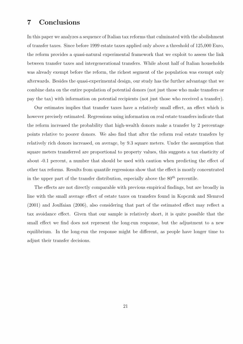
with estates above the exemption threshold of 175 thousand euro. In Figure 1 we plot the
wealth distribution in the pre-reform years 1993-1998. Since median wealth was slightly below
the exemption level (159 thousand euro), the cancellation of transfer taxes benefited more than
half of the population.
Given the change in the exemption threshold, the reform has a clear testable implication.
The post-reform tax regime should have increased the propensity to transfer of the rich (those
above the exemption level) relatively to the poor, who were already exempt before the reform.
The differential impact of the tax reforms across the wealth distribution allows us to identify
the impact of transfer taxation and to estimate the tax elasticity of intergenerational transfers
in a standard difference-in-difference framework.
9Bertocchi (2007) notices that transfer tax revenues have been declining in all OECD countries for the pastseventy years, and proposes a politico-economic model to explain this tendency. The cancellation of transfertaxes in Italy and Sweden is part of this general trend, as well as the recent policy debate and legislativeproposals in countries such as the U.S., the U.K. and France.
10In 2007 transfer taxes were reinstated after the election of the Prodi government. The exemption levels inthe reinstated taxes were quite large (one million euro per recipient), so they affected very few taxpayers. Inany case, our sample ends in 2006.
11Given that the SHIW is conducted biannually this amounts to just eliminating year 2000.
9

The only other paper that has looked at the consequences of the Italian cancellation of
transfer taxes is Bellettini and Taddei (2009). Their analysis focuses on a rather different issue,
namely the effect of the cancellation on house prices. In particular, the authors show that in
an overlapping generations model with intergenerational altruism a decrease in transfer taxes
can bring about an increase in real estate prices, and test this prediction using time series data
on house prices and real estate transfers available in 13 Italian cities. They regress the change
in house prices on city characteristics, a time trend and a post-reform dummy, and find that
the reform has induced a sizeable appreciation of residential real estate prices.
4 The data
The Survey of Household Income and Wealth (SHIW) provides a unique opportunity to test
the effect of the tax reform on the propensity to transfer. Conducted biannually by the Bank of
Italy, the survey spans pre- and post-reform years and, in each year, it is representative of the
population. Each wave includes about 8,000 households and has detailed data on economic and
demographic characteristics of household members. The survey also provides information on
dwellings owned by the household, how they were acquired (outright purchase, built to order
by the household, inherited or received as a gift) and their size (in square meters). Since gifts
and bequests are treated equally by the tax code, our definition of transfers includes both.12
Most importantly for the present study, the survey includes selected characteristics (occupation,
education, year of birth, and whether the parents are alive) of the parents of the respondent
and spouse. We assume that transfers originate from parents rather than from other relatives
or donors, and merge information on transfers with the characteristics of donors and recipients.
In the empirical analysis we focus on the 1993-2006 period in which identical questions on
transfers and the same information on respondents’ parents are available. Therefore we use
three surveys before the reform (1993-95-98) and three after (2002-04-06).
The data thus allow us to focus on the short-run effects of the removal of transfer taxes on
intergenerational transfers. We select all households in which at least one parent of the head of
the household (or of his/her spouse) is not alive at the time of the survey.13 Our final sample
12In the survey bequests and gifts are not easily distinguished in all years. Furthermore, in Italy intergener-ational gifts in the form of real estate occur rarely through formal procedures. More common is that parentsmake a cash transfer to children, who then acquire a home.
13Prior to 1993 data on donors are not available.
10
includes data on 29,900 owners of real estate wealth.
A first inspection of the data reveals that the fraction of households ever receiving real
estate as a bequest or gift was slightly below 30 percent in the pre-reform years (1993-1998),
and increased to almost 35 percent in the post-reform period (2002-06), as shown in Figure 2.
The rising trend in transfers agrees with a previous study by Cannari and D’Alessio (2008),
who find that the share of intergenerational transfers in total wealth increased from 30 to 34
percent between 1991 and 2002.
Our survey has data on transfers received over the lifetime, not receipt of a transfer in the
previous year. Therefore, a possible concern of our analysis is that the increase in reported
transfer after the reform reflects measurement error, i.e. higher reporting of transfer in most
recent years. Unfortunately, we don’t know if those interviewed after the reform report that
they received a bequest before or after the reform. To gauge the presence of measurement error,
we compute the fraction of households receiving real estate transfers for four cohorts (born in
1920-29, 1930-39, 1940-49, 1950-59). We find that the fraction of households receiving transfers
increases for each cohort between 1993 and 2006, with the exception of the two oldest cohorts
between 1993 and 1995. This pattern makes it unlikely that the increase in reported transfers
reflects measurement error rather than a genuine increase in the propensity to transfer real
estates (see Appendix B, Figure B-1).
4.1 Treatment and control group
The key feature of the reform that we exploit in the paper is that the elimination of transfer
taxes did not affect all households equally, because donors with total estates below 175 thousand
Euro were already exempt before 2000, and therefore were not affected by the tax reform. Any
impact of the reform on transfers should emerge in the group of potential donors whose estate
was above the exemption limit.
Since potential donors’ resources are not observed, we split the sample on the basis of the
donors’ occupation, which is arguably correlated with their lifetime wealth. We define as “High
parental occupation” households where at least one potential donor was either entrepreneur,
manager, professional or self-employed during his or her working life. For instance, a married
couple is classified as “High parental occupation” if any of the four potential donors is (or was
11
at the time he or she was alive) in one of the four above mentioned occupations.14 In the
empirical analysis we will also rely on a finer classification of donors’ occupation.
A major concern of our analysis is that potential donors’ occupation is only an imperfect
measure of donors’ wealth, and that our sample split is contaminated with classification errors,
that is some low-wealth donors are part of the high-occupation group and vice-versa. Although
we do not observe the correlation between wealth and occupation among potential donors we
can use information on the recipients, which is instead available, to assess if “High occupation”
households (at least one member in a high-occupation) are wealthier than “Low occupation”
households. In 1993-2006 the average wealth difference between the two groups is 214 thousand
Euro (the difference in medians is 111 thousand Euro). The difference is also stable across years,
lending support to our assumption that the sample split based on donors’ occupation is strongly
correlated with their unobserved resources.15
Several results further corroborate our assumption. Wealth regressions indicate that “High
occupation” is a strong predictor of wealth, even conditioning on age, education, gender, family
size, area of residence, income quartile dummies and year dummies. The estimated coefficients
range from 155 to 214 thousand Euro, see Appendix B, Table B-1. Cross-tabulating occupation
by the wealth threshold (above or below 175,000), we find that 55 percent of “Low occupation”
households have wealth below the threshold, while 69.4 percent of “High occupation” households
are above. Probit estimates for the probability of being above the threshold confirm that
occupation is a strong predictor of wealth: the marginal effect ranges from 16 to 25 percent,
depending on the specification (Appendix B, Table B-2).
Evidence on the wealth distribution in the sample of recipients suggests that wealth and
occupation are strongly correlated, but does not rule out that misclassification affects our sam-
ple split of donors. To address this issue we control for additional variables which potentially
affect the membership to the treatment group. Second, we show that under mild conditions
the estimated transfer effect of the tax reform is a lower bound of the true effect (see Sec-
tion 6.1 and Appendix C). Finally, we exploit the fact that the effect of the reform should
be stronger among those who are substantially above the threshold. Therefore, we further
14Of course, other classifications are possible, and indeed we report sensitivity analysis on alternative groupdefinitions (see Section 6).
15The assumption that transfers originates from parents may introduce some measurement error in transfers,but our estimates will still be valid if the error applies equally to the two groups (high and low occupations).
12
distinguish “High parental occupation” households into “Exactly one high” and “At least two
high parental occupations”, depending on whether just one or at least two parents are in a
high occupation. Under the assumption that occupation is a good predictor of wealth, as the
evidence on recipients seems to confirm, one should expect a larger effect of the reform on the
“At least two high parental occupations” households.
4.2 Descriptive analysis
In Figure 3 we report a breakdown of the fraction of households receiving transfers from high-
and low-occupation donors. In the pre-reform period (1993-1998), the fraction was, on average,
32 percent, vis-a-vis 26 percent in the low-occupation group. After the reform (2002-2006)
the fraction increased to 41 percent in the high-occupation group, against 32 percent in the
low-occupation group. Thus, the difference between high- and low-occupation donors increased
by 3 percentage points after the reform.
In Figure 4 we report the same breakdown for the square meters transferred. Before the
sequence of reforms, high-occupation donors transferred, on average, 48 square meters (149
among those who actually made a transfer), while low-occupation donors 30 (respectively, 118)
square meters. After the reforms, square meters transferred increased to 66 (162) and 37 (116),
respectively. Thus, after the reforms the difference between the two groups increased by 11 (15)
square meters. The descriptive analysis suggests that the tax change did not affect equally all
potential donors, but seems to have affected high-occupation donors to a larger extent.
Table 2 provides summary statistics of the variables used in the estimation by donors’
occupation: fraction of households ever receiving real estate transfers, square meters transferred,
donors’ and recipients’ characteristics. Not surprisingly, high-occupation donors tend to have
higher education as well, while donors’ birth cohort does not differ significantly between high-
and low-occupation groups. As for recipients’ characteristics, the last rows of Table 2 show
that households with high-occupation donors are more likely to be males, and have higher
income and education. Thus, as expected, treatment and control groups differ along important
characteristics, such as donor’s education and recipients’ gender, education and income. In the
empirical analysis we will be able to control for differences in treatment and control groups
due to time-invariant variables, such as gender, education and cohort. The next section further
discusses how we control for residual heterogeneity between the two groups in our difference-
13
in-difference estimates.
5 The empirical framework
We assume that the transfer decision of parent i in period t depends on parent’s lifetime wealth
net of taxes (1− τ)wp, parent’s characteristics xp, children’s lifetime wealth wk, and children’s
characteristics xk:
Y ∗it = ζ0,p(1− τt)wpi + xpi ζ1,p + ζ0,kw
ki + xki ζ1,k + uit (1)
The variable Y ∗it reflects the difference between the indirect utility of transferring wealth
and the utility of not transferring, and it is not directly observed. Instead, we have data on
whether a real estate was transferred over the lifetime, and the square meters transferred.
As explained in Section 3, the reform provides an exogenous source of variation that we
exploit to assess the causal link between taxes and intergenerational transfers in a quasi-
experimental setting. Thus, we express equation (1) in a standard difference-in-difference
framework, distinguishing between tax-payers affected by the reform (the treatment group that
includes high-occupation donors) and unaffected taxpayers (the control group that includes
donors with low-occupation). We assume that potential donors in the treatment group face
an exogenous and unexpected reduction in transfer taxes, and check how their propensity to
transfer changes relative to the donors in the control group.16
We make equation (1) operational pooling data from pre and post-reform periods and esti-
mating the following equation:
Yit = α + βMi + γPOSTt + δMi × POSTt + xpi ζp + xki ζ
k + εit (2)
We estimate equation (2) using two outcome variables: a dummy variable equal to 1 if a real
estate was ever transferred and the log of square meters transferred. The two outcomes capture
the extensive and the intensive margins of our measure of transfers. On the right hand side,
Mi is a dummy equal to 1 for high-wealth parents (measured as high occupation); POSTt is a
dummy for the post-reform period; xpi includes time-invariant parents’ characteristics (education
16Since our sample is relatively short, the estimates are not able to capture the long-run (steady-state) effectsof the tax reform.
14
and cohort dummies), and xki recipients’ characteristics (gender, area of residence, education
and cohort dummies).17
In equation (2) the coefficient β measures the difference in the propensity to transfer between
high and low-wealth parents. The coefficient γ measures the difference in the propensity to
transfer after the reform for both groups. Our main coefficient of interest (δ) reflects the
differential effect of the reform between the two groups. A positive δ reflects larger transfers
from high-wealth parents after the reform, while a value of δ equal to zero indicates that the
reform does not have any effect on transfers.
In order to evaluate the effect of the reform on the extensive margin, we estimate a linear
probability model. The reason is that all covariates in equation (2) are dummy variables. When
the right-hand side variables are discrete, the linear probability model is completely general and
the fitted probabilities lie within the interval [0, 1].18 In addition to being completely general
in this context, the linear probability model also has the advantage of allowing a straightfor-
ward interpretation of the regression coefficients. Since the error term of the linear model is
heteroskedastic, standard errors are computed using White (1980) heteroskedasticity-robust
variance matrix. Finally, to evaluate the effect of the reform on the intensive margin, we rely
on a standard tobit model for square meter transferred, which allows us to compute the effect
both conditional on making a transfer as well as the unconditional expected value of square
meter transferred.
The diff-in-diff approach controls for any time-invariant differences between treatment and
control groups. As discussed in Section 4, Figures 3 and 4 provide visual support for the
assumption that pre-reform trends in outcomes are the same for treatment and control groups.
Of course, we still need to assume that other time-varying factors that we have possibly omitted
do not affect the two groups differentially, acting as confounding variables. For this reason,
in some specifications we also include the (log) of recipients’ disposable income. While this
may be rightly criticized because recipients’ income is likely to be endogenous with respect to
the transfer decision, it is important to check that the results are robust to the inclusion of
time-varying controls that are correlated with unobserved heterogeneity.
17We disregard recipients’ characteristics that are not observable by potential donors at the time of thetransfer. For this reason, in our baseline specification we don’t include recipients’ resources.
18In this case, the fitted probabilities are simply the averages of the dependent variable within each celldefined by the different values of the covariates (Angrist, 2001; Wooldridge, 2001).
15
6 The effect of the tax reform on transfers
In this section we report regression results from the estimation of equation (2) to assess the
effect of the sequence of tax reforms on whether any dwellings was transferred and on the size
of the transfers measured in square meters. Our approach thus investigates both the extensive
and the intensive margins through which the tax reforms might have affected donors’ decisions.
6.1 Extensive margin
Table 3 reports the results from estimating the linear probability model for whether a dwelling
was transferred. High-occupation donors are the treatment group, the group of households in
which at least one parent of the head and spouse (if present) is an entrepreneur, manager,
professional or self-employed. The first column of Table 3 reports the results for the baseline
specification, where we condition only on donors’ occupation, a full set of time-dummies, and
the interaction between the treatment group dummy (dummy for high-occupation donors) and
a dummy that is equal to one for 2002-06.19
Consistently with the evidence in Figure 3, the results show that the propensity to transfer
real estate wealth is significantly higher for high-occupation donors. The coefficient of the
interaction between the high-occupation dummy and the post-reform dummy shows that the
probability of making a transfer increased by 2.5 percentage points for high- relative to low-
occupation donors after the reform.20
As noticed, misclassification errors between treatment and control groups can bias the esti-
mated effect of the reform downward.21 If the wealth distribution of recipients exactly matched
the donors’ distribution, we could readily estimate the probabilities of correct classification and
the magnitude of the bias. Since the two distributions are likely to be different, we assume
that the ranks of the wealth distribution of recipients differ from those of donors by random
slippages.22 Appendix C shows that under very mild conditions the estimated coefficient pro-
19Introducing a full set of time dummies in the estimation rather than the more restrictive dummy for post-reform years leaves the results unchanged. The coefficients of the time dummies confirm the pattern of transfersapparent from Figure 3. The effect of time is non-linear and peaks in 2004, two years after the abolition of theestate tax.
20Before the reform the probability of transferring real estate wealth for the high occupation donors was 32percent.
21Aigner (1973) shows that if a binary covariate is measured with error the least square coefficient is asymp-totically downward biased if misclassification errors are not too large. Mahajan (2006), Lewbel (2007) andBattistin and Sianesi (2011) obtain the same result in different settings.
22Battistin and Sianesi (2011) follow a similar approach in the exploration of the effect of mismeasured
16
vides a lower bound of the true effect. For instance, if the estimated coefficient is 0.025 and the
probabilities of correct classification in the treatment and control groups are 85% and 80%, re-
spectively, the true effect is 0.038.23 Notice that whatever the misclassification error, a positive
coefficient implies that the reform does affect transfers.
The evidence in Section 4.1 suggests that other variables are correlated with wealth and can
affect the assignment to the treatment group based on occupation only. Therefore, in Table
3 we expand the baseline specification with additional variables. In column 2 we control for
other donors’ characteristics (education and cohort). In column 3 we further include recipients’
characteristics (gender, area of residence, education and cohort). The results show that males
are less likely to receive a transfer, that the probability of receiving a transfer is higher in the
South and for younger generations (born after 1950). In the final column we add the (log) of
recipients’ disposable income. Notice that current income is not observable by donors at the
time of the transfer. Additionally, as discussed above, income is likely to be endogenous, as
transfers may affect future recipients’ income. For these reasons, we cautiously include income
only in the last specification to capture unobserved recipients’ characteristics that may affect
donors’ behavior. Our coefficient of interest is always positive and significant and is quite stable
across specifications, ranging from 2.1 to 2.2 percent.24
To further explore the consequences of misclassification, we adopt a sharper identification of
the treatment group, as discussed in Section 4.1. The results are presented in Table 4, where we
interact the post-reform dummy with a dummy for “At least two high parental occupations”,
equal to one for households in which at least two parents of the head and spouse (if present) are
entrepreneurs, managers, professionals or self-employed. In other words, we further split the
high-occupation sample into two groups: “Exactly one high” and “At least two high parental
occupations”. As the incentive to transfer wealth after the reform is directly related to the level
of donors’ wealth, the effect of the reform should be larger for the latter group.
schooling on the estimated returns to education. They bound the true effect of education on earnings assumingthat the sum of type I and II errors ranges from 10 to 40 percent.
23Figure C-1 in Appendix C reports the true effect as a function of the two classification errors when theestimated coefficient is 0.025. The bias increases with the amount of misclassification. For high values ofmisclassification errors (25% in each of the two groups), the true effect is about 2 times the estimated effect.
24Given that Figure B-1 points to possible measurement error for some cohorts in 1993, we check the robustnessof our results removing the 1993 survey. Table B-3 in Appendix B shows that the effects of the reform arequalitatively unchanged and even larger in magnitude. To control for possible changes in the composition ofthe sample, we perform a number of additional checks available upon request. In particular, we include in theregression the cohort dummies for the spouse, we exclude from the sample recipients with wealth below the firstor second deciles and we exclude from the sample households with only one high-occupation parent.
17
The results show that this is indeed the case. In the baseline specification, reported in the
first column of Table 4, the coefficient of the interaction with the “Exactly one high occupa-
tion” dummy drops to 1.1 percentage points, while that of the interaction with the “At least
two high parental occupations” dummy implies that for this group the propensity to transfer
increases by 4.8 points. Controlling for donors’ and recipients’ characteristics does not alter
the overall picture, and confirms the presence of a positive and statistically detectable effect of
the tax changes on transfers. Additionally, including this finer classification of donors further
corroborates our identification strategy, and agrees with the idea that the effect of the reform
rises with donors’ wealth.25
6.2 Intensive margin
In Table 5 we use a standard Tobit-I model, which allows to decompose the effect of the reform
into the effect on the amount transferred, given that a transfer takes place, and the effect on
the probability of transferring.26 The first regression of Table 5 indicates that the coefficient
of the high parental occupation dummy is positive, indicating that wealthier donors make
larger transfers. The interaction between the post-reform and the high occupation dummy
is also positive and precisely estimated, suggesting that the tax reform increased the amount
transferred.
The lower panel of Table 5 reports marginal effects, showing that the tax reform increased
transfers by 9.3 square meters. The increase can be decomposed in the effect on the amount
transferred, given that a transfer takes place (6.4 square meters), and the effect on the proba-
bility of making a transfer (0.036).27 Even though the nature of the reform does not allow us
to compute a proper tax elasticity of bequests, we can still provide a calculation that gives a
sense of the magnitude of the estimated effect. Since transfers increase by 9.3 percent, which
is about 10 percent of the median transfer, and since the reform brings about a 100 percent
reduction of the tax rate, our results imply that the tax elasticity of square meters transferred
is in the range of -0.1 percent. Under the strong assumption that square meters transferred
25Using an alternative classification, based on exactly one, exactly 2, exactly 3, and exactly 4 high occupations(the category no high occupation is the reference group) does not change the results.
26This is the McDonald and Moffit (1980) decomposition.27Since the control variables are dummies, the marginal effects are the discrete changes of square meters
transferred for the high occupation group after the reform. Appendix D shows how we compute marginal effectsand their associated standard errors.
18
are proportional to property values, the size of the elasticity is consistent with the evidence of
Joulfaian (2006) in a rather different context. This number should be interpreted with great
care not only because it reflects the evaluation of the marginal effect of the Tobit at the mean
of the transfers distribution, but also and foremost because it is based on the assumption that
the tax elasticity is constant. In fact, our quasi-experimental exercise, provides an exogenous
source of variation of the tax rate, but prevents us to test if the tax elasticity of transfers
varies along the tax schedule. This implies that our evidence should be used with caution when
predicting the effect of other tax reforms.
In columns 2, 3 and 4 we add donors’ and recipients’ characteristics to the baseline specifica-
tion. The interaction term remains positive and significant, but the marginal effects imply now
a smaller effect of the reform on square meters. The results on the recipients characteristics
parallel those reported in Table 3. Highly educated recipients, residents in the South, females
and younger recipients receive larger transfers.
Table 6 splits the treatment group into “Exactly one” and “At least two high parental occu-
pations” groups. The coefficients of the interaction between the post-reform and the “Exactly
one” dummies are smaller than the corresponding coefficients in Table 5 and not statistically
different from zero. Instead, the coefficients of the interaction term with “At least two high
parental occupations” are larger than in Table 5. The marginal effects range from 14.9 (column
4) to 17.3 (column 1), and the implied tax-elasticity for this group is -0.17 to -0.14 percent at
the median.
So far the analysis has focused on the impact of the reform on average transfer. However,
the effect of the reform is likely to vary along the distribution of transfers. In particular,
one would expect the effect to be larger in the upper part of the distribution, because higher
transfers were taxed at increasingly higher rates due to the progressive structure of the pre-
reform legislation. Figure 5 compares the empirical cumulative distribution function of transfers
for high-occupation households with the same distribution had the reform not canceled the tax
(the counterfactual distribution).28 The figure shows that the reform had no effect for most
part of the distribution, and that the effect is mostly concentrated between the percentiles 70%
28To obtain the counterfactual distribution of transfers, we proceed as follows. We add the q-percentile ofdistribution of transfers in the treatment group before the reform to the difference between the inverse of thedistribution of transfers in the control group with respect q after and before the reform. More details can befound in Appendix E and in Athey and Imbens (2006), who discuss identification and inference in non-lineardifference-in-difference models.
19

to 95% of the transfers distribution.
Table 7 further investigates the issue running quantile regressions. The results show that
the impact of the cancellation of transfer taxes increases along the transfer distribution. In
particular, column 1 indicates no significant effect of the reform at the 80th percentile, while
the impact shows up positive and significant at the 85th, with a coefficient of 11.1 (column 2),
the 90th percentile (22.9), and the 95th percentile (34.8).
Overall, our econometric evidence suggests that the abolition of transfer taxes that took
place between 1999 and 2001 has increased real estate transfers. The effect is rather small, but
precisely estimated. Furthermore, the evidence shows that wealthier donors have been affected
the most. In principle, the evidence does not rule out that the increase in transfers reflects a
change in the composition of transfers (a tax avoidance effect), a change in reported transfers,
or a combination of the two. As for the tax avoidance effect, it might be that after the reform
donors were more willing to transfer wealth in the form of real estate rather than in the form
of financial wealth, which before the reform was more easily hidden to tax authorities. Since
in Italy real estate assets represent 86 percent of total wealth for those aged 60 and above, we
find it plausible that at least part of the increase in real estate transfers represents a genuine
tax effect.29
Our estimates should be interpreted with care also because after the reform some recipients
might be more willing to declare that they have received a real transfer in the past.30 We see no
particular reason why changes in reporting should affect more than proportionally individuals
who received transfers from high-wealth donors. Furthermore, cohort profiles show that the
proportion reporting transfers increases for all cohorts around the time of the reform. We
take this as indirect evidence that the increase in reported transfers is not due to a change in
reporting behavior, but to a genuine increase in the propensity to transfer.31
29Furthermore, a special section of SHIW on intergenerational transfers for 1991 and 2002 signals an increasein total transfers (real plus financial), see Cannari and D’Alessio (2008). Data on parents’ occupation oreducation is not available in 1991.
30Gorodnichenko et al. (2009) report evidence from Russian survey data suggesting that people underreportincome to survey takers for fear of tipping off the tax authorities.
31The profiles are constructed creating pseudo-panels based on the year of birth of the households head andare plotted in Figure B-1 of Appendix B.
20
7 Conclusions
In this paper we analyzes a sequence of Italian tax reforms that culminated with the abolishment
of transfer taxes. Since before 1999 estate taxes applied only above a threshold of 125,000 Euro,
the reform provides a quasi-natural experimental framework that we exploit to assess the link
between transfer taxes and intergenerational transfers. While about half of Italian households
was already exempt before the reform, the richest segment of the population was exempt only
afterwards. Besides the quasi-experimental design, our study has the further advantage that we
combine data on the entire population of potential donors (not just those who make transfers or
pay the tax) with information on potential recipients (not just those who received a transfer).
Our estimates implies that transfer taxes have a relatively small effect, an effect which is
however precisely estimated. Regressions using information on real estate transfers indicate that
the reform increased the probability that high-wealth donors make a transfer by 2 percentage
points relative to poorer donors. We also find that after the reform real estate transfers by
relatively rich donors increased, on average, by 9.3 square meters. Under the assumption that
square meters transferred are proportional to property values, this suggests a tax elasticity of
about -0.1 percent, a number that should be used with caution when predicting the effect of
other tax reforms. Results from quantile regressions show that the effect is mostly concentrated
in the upper part of the transfer distribution, especially above the 80th percentile.
The effects are not directly comparable with previous empirical findings, but are broadly in
line with the small average effect of estate taxes on transfers found in Kopczuk and Slemrod
(2001) and Joulfaian (2006), also considering that part of the estimated effect may reflect a
tax avoidance effect. Given that our sample is relatively short, it is quite possible that the
small effect we find does not represent the long-run response, but the adjustment to a new
equilibrium. In the long-run the response might be different, as people have longer time to
adjust their transfer decisions.
21
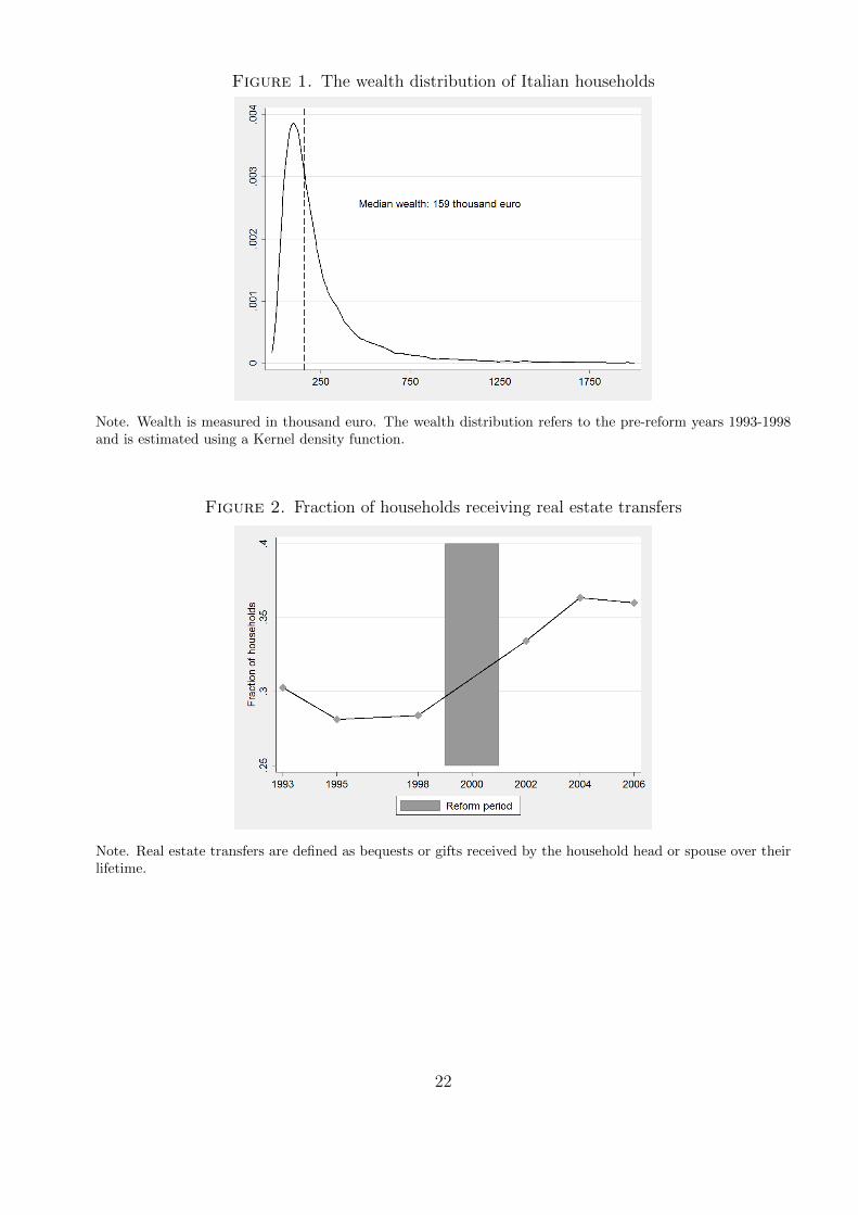
Figure 1. The wealth distribution of Italian households
Note. Wealth is measured in thousand euro. The wealth distribution refers to the pre-reform years 1993-1998and is estimated using a Kernel density function.
Figure 2. Fraction of households receiving real estate transfers
Note. Real estate transfers are defined as bequests or gifts received by the household head or spouse over theirlifetime.
22
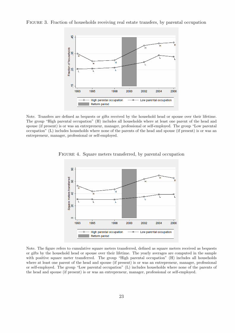
Figure 3. Fraction of households receiving real estate transfers, by parental occupation
Note. Transfers are defined as bequests or gifts received by the household head or spouse over their lifetime.The group “High parental occupation” (H) includes all households where at least one parent of the head andspouse (if present) is or was an entrepreneur, manager, professional or self-employed. The group “Low parentaloccupation” (L) includes households where none of the parents of the head and spouse (if present) is or was anentrepreneur, manager, professional or self-employed.
Figure 4. Square meters transferred, by parental occupation
Note. The figure refers to cumulative square meters transferred, defined as square meters received as bequestsor gifts by the household head or spouse over their lifetime. The yearly averages are computed in the samplewith positive square meter transferred. The group “High parental occupation” (H) includes all householdswhere at least one parent of the head and spouse (if present) is or was an entrepreneur, manager, professionalor self-employed. The group “Low parental occupation” (L) includes households where none of the parents ofthe head and spouse (if present) is or was an entrepreneur, manager, professional or self-employed.
23
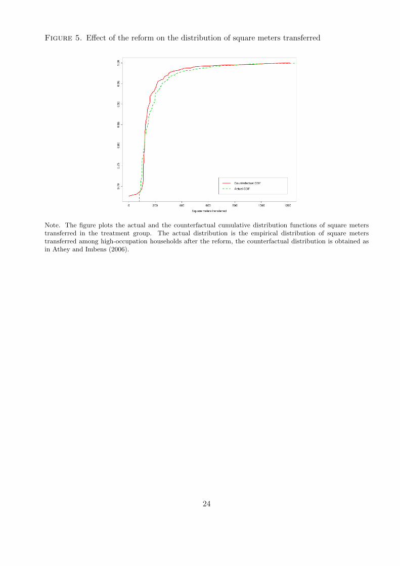
Figure 5. Effect of the reform on the distribution of square meters transferred
Note. The figure plots the actual and the counterfactual cumulative distribution functions of square meterstransferred in the treatment group. The actual distribution is the empirical distribution of square meterstransferred among high-occupation households after the reform, the counterfactual distribution is obtained asin Athey and Imbens (2006).
24

Table 1. The reforms of transfer taxation in Italy
Tax Base Exemption Tax rate Note
Law346/1990
Total donor’s es-tate
125,000 euro fortotal estate
Brackets(’000 euros)125-175175-250250-400400-750750-15001500+
Tax Rate
3710152227
An additional progressivetax is levied on the shareof the estate received byrecipients who are not di-rect relatives of the donoror spouse. For gifts thesame tax rates apply.
Law488/1999
Total donor’s es-tate
175,000 euro fortotal estate
Brackets(’000 euros)175-250250-400400-750750-15001500+
Tax Rate
710152227
An additional progressivetax is levied on the shareof the estate received byrecipients who are not di-rect relatives of the donoror spouse. For gifts thesame tax rates apply.
Law342/2000
Estate share re-ceived by eachrecipient
175,000 euro foreach recipient
Flat tax rate: 4% forspouse and direct rela-tives, 6% for relatives upto fourth degree, 8% forothers
For gifts: 3%, 5% and 7%respectively.
Law383/2001
The inheritancetax was abol-ished
Abolished
Law296/2007
Estate share re-ceived by eachrecipient
1 million eurofor each recipi-ent
Flat tax rate: 4% forspouse and direct rela-tives, 6% for relatives upto fourth degree, 8% forothers
For gifts the same taxrates apply.
25
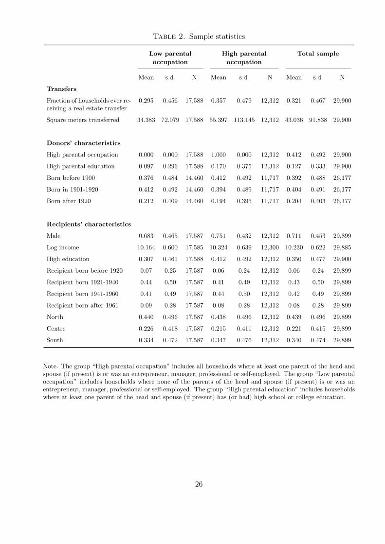
Table 2. Sample statistics
Low parental High parental Total sample
occupation occupation
Mean s.d. N Mean s.d. N Mean s.d. N
Transfers
Fraction of households ever re-ceiving a real estate transfer
0.295 0.456 17,588 0.357 0.479 12,312 0.321 0.467 29,900
Square meters transferred 34.383 72.079 17,588 55.397 113.145 12,312 43.036 91.838 29,900
Donors’ characteristics
High parental occupation 0.000 0.000 17,588 1.000 0.000 12,312 0.412 0.492 29,900
High parental education 0.097 0.296 17,588 0.170 0.375 12,312 0.127 0.333 29,900
Born before 1900 0.376 0.484 14,460 0.412 0.492 11,717 0.392 0.488 26,177
Born in 1901-1920 0.412 0.492 14,460 0.394 0.489 11,717 0.404 0.491 26,177
Born after 1920 0.212 0.409 14,460 0.194 0.395 11,717 0.204 0.403 26,177
Recipients’ characteristics
Male 0.683 0.465 17,587 0.751 0.432 12,312 0.711 0.453 29,899
Log income 10.164 0.600 17,585 10.324 0.639 12,300 10.230 0.622 29,885
High education 0.307 0.461 17,588 0.412 0.492 12,312 0.350 0.477 29,900
Recipient born before 1920 0.07 0.25 17,587 0.06 0.24 12,312 0.06 0.24 29,899
Recipient born 1921-1940 0.44 0.50 17,587 0.41 0.49 12,312 0.43 0.50 29,899
Recipient born 1941-1960 0.41 0.49 17,587 0.44 0.50 12,312 0.42 0.49 29,899
Recipient born after 1961 0.09 0.28 17,587 0.08 0.28 12,312 0.08 0.28 29,899
North 0.440 0.496 17,587 0.438 0.496 12,312 0.439 0.496 29,899
Centre 0.226 0.418 17,587 0.215 0.411 12,312 0.221 0.415 29,899
South 0.334 0.472 17,587 0.347 0.476 12,312 0.340 0.474 29,899
Note. The group “High parental occupation” includes all households where at least one parent of the head andspouse (if present) is or was an entrepreneur, manager, professional or self-employed. The group “Low parentaloccupation” includes households where none of the parents of the head and spouse (if present) is or was anentrepreneur, manager, professional or self-employed. The group “High parental education” includes householdswhere at least one parent of the head and spouse (if present) has (or had) high school or college education.
26
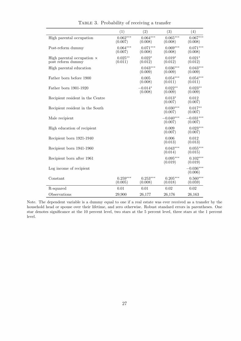
Table 3. Probability of receiving a transfer
(1) (2) (3) (4)
High parental occupation 0.062∗∗∗ 0.064∗∗∗ 0.065∗∗∗ 0.067∗∗∗
(0.007) (0.008) (0.008) (0.008)
Post-reform dummy 0.064∗∗∗ 0.071∗∗∗ 0.069∗∗∗ 0.071∗∗∗
(0.007) (0.008) (0.008) (0.008)
High parental occupation Ö 0.025∗∗ 0.022∗ 0.019∗ 0.021∗
post reform dummy (0.011) (0.012) (0.012) (0.012)
High parental education 0.043∗∗∗ 0.036∗∗∗ 0.043∗∗∗
(0.009) (0.009) (0.009)
Father born before 1900 0.005 0.054∗∗∗ 0.054∗∗∗
(0.008) (0.011) (0.011)
Father born 1901-1920 −0.014∗ 0.022∗∗ 0.023∗∗
(0.008) (0.009) (0.009)
Recipient resident in the Centre 0.013∗ 0.012(0.007) (0.007)
Recipient resident in the South 0.030∗∗∗ 0.017∗∗
(0.007) (0.007)
Male recipient −0.040∗∗∗ −0.031∗∗∗
(0.007) (0.007)
High education of recipient 0.009 0.023∗∗∗
(0.007) (0.007)
Recipient born 1921-1940 0.006 0.012(0.013) (0.013)
Recipient born 1941-1960 0.043∗∗∗ 0.055∗∗∗
(0.014) (0.015)
Recipient born after 1961 0.095∗∗∗ 0.102∗∗∗
(0.019) (0.019)
Log income of recipient −0.036∗∗∗
(0.006)
Constant 0.259∗∗∗ 0.253∗∗∗ 0.205∗∗∗ 0.560∗∗∗
(0.005) (0.008) (0.018) (0.059)
R-squared 0.01 0.01 0.02 0.02
Observations 29,900 26,177 26,176 26,163
Note. The dependent variable is a dummy equal to one if a real estate was ever received as a transfer by thehousehold head or spouse over their lifetime, and zero otherwise. Robust standard errors in parentheses. Onestar denotes significance at the 10 percent level, two stars at the 5 percent level, three stars at the 1 percentlevel.
27
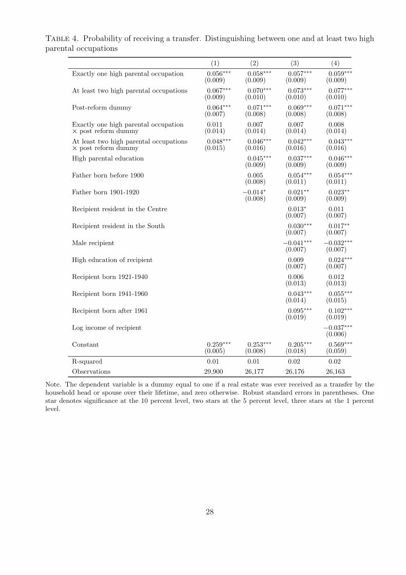
Table 4. Probability of receiving a transfer. Distinguishing between one and at least two highparental occupations
(1) (2) (3) (4)
Exactly one high parental occupation 0.056∗∗∗ 0.058∗∗∗ 0.057∗∗∗ 0.059∗∗∗
(0.009) (0.009) (0.009) (0.009)
At least two high parental occupations 0.067∗∗∗ 0.070∗∗∗ 0.073∗∗∗ 0.077∗∗∗
(0.009) (0.010) (0.010) (0.010)
Post-reform dummy 0.064∗∗∗ 0.071∗∗∗ 0.069∗∗∗ 0.071∗∗∗
(0.007) (0.008) (0.008) (0.008)
Exactly one high parental occupation 0.011 0.007 0.007 0.008Ö post reform dummy (0.014) (0.014) (0.014) (0.014)
At least two high parental occupations 0.048∗∗∗ 0.046∗∗∗ 0.042∗∗∗ 0.043∗∗∗
Ö post reform dummy (0.015) (0.016) (0.016) (0.016)
High parental education 0.045∗∗∗ 0.037∗∗∗ 0.046∗∗∗
(0.009) (0.009) (0.009)
Father born before 1900 0.005 0.054∗∗∗ 0.054∗∗∗
(0.008) (0.011) (0.011)
Father born 1901-1920 −0.014∗ 0.021∗∗ 0.023∗∗
(0.008) (0.009) (0.009)
Recipient resident in the Centre 0.013∗ 0.011(0.007) (0.007)
Recipient resident in the South 0.030∗∗∗ 0.017∗∗
(0.007) (0.007)
Male recipient −0.041∗∗∗ −0.032∗∗∗
(0.007) (0.007)
High education of recipient 0.009 0.024∗∗∗
(0.007) (0.007)
Recipient born 1921-1940 0.006 0.012(0.013) (0.013)
Recipient born 1941-1960 0.043∗∗∗ 0.055∗∗∗
(0.014) (0.015)
Recipient born after 1961 0.095∗∗∗ 0.102∗∗∗
(0.019) (0.019)
Log income of recipient −0.037∗∗∗
(0.006)
Constant 0.259∗∗∗ 0.253∗∗∗ 0.205∗∗∗ 0.569∗∗∗
(0.005) (0.008) (0.018) (0.059)
R-squared 0.01 0.01 0.02 0.02
Observations 29,900 26,177 26,176 26,163
Note. The dependent variable is a dummy equal to one if a real estate was ever received as a transfer by thehousehold head or spouse over their lifetime, and zero otherwise. Robust standard errors in parentheses. Onestar denotes significance at the 10 percent level, two stars at the 5 percent level, three stars at the 1 percentlevel.
28
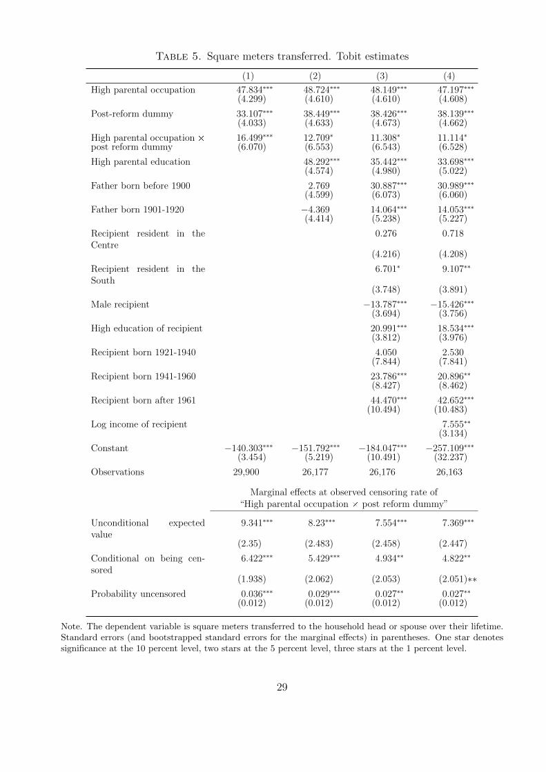
Table 5. Square meters transferred. Tobit estimates
(1) (2) (3) (4)
High parental occupation 47.834∗∗∗ 48.724∗∗∗ 48.149∗∗∗ 47.197∗∗∗
(4.299) (4.610) (4.610) (4.608)
Post-reform dummy 33.107∗∗∗ 38.449∗∗∗ 38.426∗∗∗ 38.139∗∗∗
(4.033) (4.633) (4.673) (4.662)
High parental occupation Ö 16.499∗∗∗ 12.709∗ 11.308∗ 11.114∗
post reform dummy (6.070) (6.553) (6.543) (6.528)
High parental education 48.292∗∗∗ 35.442∗∗∗ 33.698∗∗∗
(4.574) (4.980) (5.022)
Father born before 1900 2.769 30.887∗∗∗ 30.989∗∗∗
(4.599) (6.073) (6.060)
Father born 1901-1920 −4.369 14.064∗∗∗ 14.053∗∗∗
(4.414) (5.238) (5.227)
Recipient resident in theCentre
0.276 0.718
(4.216) (4.208)
Recipient resident in theSouth
6.701∗ 9.107∗∗
(3.748) (3.891)
Male recipient −13.787∗∗∗ −15.426∗∗∗
(3.694) (3.756)
High education of recipient 20.991∗∗∗ 18.534∗∗∗
(3.812) (3.976)
Recipient born 1921-1940 4.050 2.530(7.844) (7.841)
Recipient born 1941-1960 23.786∗∗∗ 20.896∗∗
(8.427) (8.462)
Recipient born after 1961 44.470∗∗∗ 42.652∗∗∗
(10.494) (10.483)
Log income of recipient 7.555∗∗
(3.134)
Constant −140.303∗∗∗ −151.792∗∗∗ −184.047∗∗∗ −257.109∗∗∗
(3.454) (5.219) (10.491) (32.237)
Observations 29,900 26,177 26,176 26,163
Marginal effects at observed censoring rate of“High parental occupation Ö post reform dummy”
Unconditional expectedvalue
9.341∗∗∗ 8.23∗∗∗ 7.554∗∗∗ 7.369∗∗∗
(2.35) (2.483) (2.458) (2.447)
Conditional on being cen-sored
6.422∗∗∗ 5.429∗∗∗ 4.934∗∗ 4.822∗∗
(1.938) (2.062) (2.053) (2.051)∗∗Probability uncensored 0.036∗∗∗ 0.029∗∗∗ 0.027∗∗ 0.027∗∗
(0.012) (0.012) (0.012) (0.012)
Note. The dependent variable is square meters transferred to the household head or spouse over their lifetime.Standard errors (and bootstrapped standard errors for the marginal effects) in parentheses. One star denotessignificance at the 10 percent level, two stars at the 5 percent level, three stars at the 1 percent level.
29
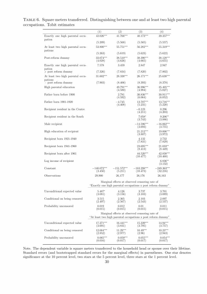
Table 6. Square meters transferred. Distinguishing between one and at least two high parentaloccupations. Tobit estimates
(1) (2) (3) (4)
Exactly one high parental occu-pation
42.026∗∗∗ 41.766∗∗∗ 40.173∗∗∗ 39.357∗∗∗
(5.209) (5.568) (5.565) (5.557)
At least two high parental occu-pations
53.800∗∗∗ 55.751∗∗∗ 56.282∗∗∗ 55.319∗∗∗
(5.263) (5.619) (5.623) (5.622)
Post-reform dummy 33.074∗∗∗ 38.510∗∗∗ 38.390∗∗∗ 38.128∗∗∗
(4.028) (4.626) (4.665) (4.655)
Exactly one high parental occu-pation
7.578 3.459 2.847 2.947
Ö post reform dummy (7.326) (7.834) (7.820) (7.802)
At least two high parental occu-pations
31.602∗∗∗ 28.338∗∗∗ 26.171∗∗∗ 25.638∗∗∗
Ö post reform dummy (7.903) (8.406) (8.393) (8.378)
High parental education 49.791∗∗∗ 36.996∗∗∗ 35.405∗∗∗
(4.580) (4.984) (5.027)
Father born before 1900 2.781 30.836∗∗∗ 30.911∗∗∗
(4.592) (6.064) (6.052)
Father born 1901-1920 −4.745 13.707∗∗∗ 13.716∗∗∗
(4.408) (5.231) (5.220)
Recipient resident in the Centre −0.123 0.296(4.211) (4.203)
Recipient resident in the South 7.058∗ 9.206∗∗
(3.743) (3.886)
Male recipient −14.596∗∗∗ −16.062∗∗∗
(3.693) (3.755)
High education of recipient 21.212∗∗∗ 19.006∗∗∗
(3.807) (3.972)
Recipient born 1921-1940 4.132 2.732(7.831) (7.829)
Recipient born 1941-1960 23.695∗∗∗ 21.033∗∗
(8.413) (8.449)
Recipient born after 1961 44.520∗∗∗ 42.838∗∗∗
(10.477) (10.468)
Log income of recipient 6.836∗∗
(3.132)
Constant −140.072∗∗∗ −151.572∗∗∗ −183.298∗∗∗ −249.363∗∗∗
(3.450) (5.211) (10.473) (32.216)
Observations 29,900 26,177 26,176 26,163
Marginal effects at observed censoring rate of“Exactly one high parental occupations x post reform dummy”
Unconditional expected value 5.487∗ 4.126 3.737 3.701(3.081) (3.156) (3.103) (3.089)
Conditional on being censored 3.515 2.365 2.103 2.097(2.497) (2.567) (2.543) (2.537)
Probability uncensored 0.019 0.012 0.01 0.011(0.015) (0.015) (0.015) (0.015)
Marginal effects at observed censoring rate of“At least two high parental occupations x post reform dummy”
Unconditional expected value 17.271∗∗∗ 16.441∗∗∗ 15.339∗∗∗ 14.94∗∗∗
(3.691) (3.831) (3.795) (3.757)
Conditional on being censored 12.084∗∗∗ 11.29∗∗∗ 10.49∗∗∗ 10.23∗∗∗
(2.852) (2.977) (2.96) (2.943)
Probability uncensored 0.065∗∗∗ 0.059∗∗∗ 0.055∗∗∗ 0.054∗∗∗
(0.016) (0.017) (0.017) (0.017)
Note. The dependent variable is square meters transferred to the household head or spouse over their lifetime.Standard errors (and bootstrapped standard errors for the marginal effects) in parentheses. One star denotessignificance at the 10 percent level, two stars at the 5 percent level, three stars at the 1 percent level.
30
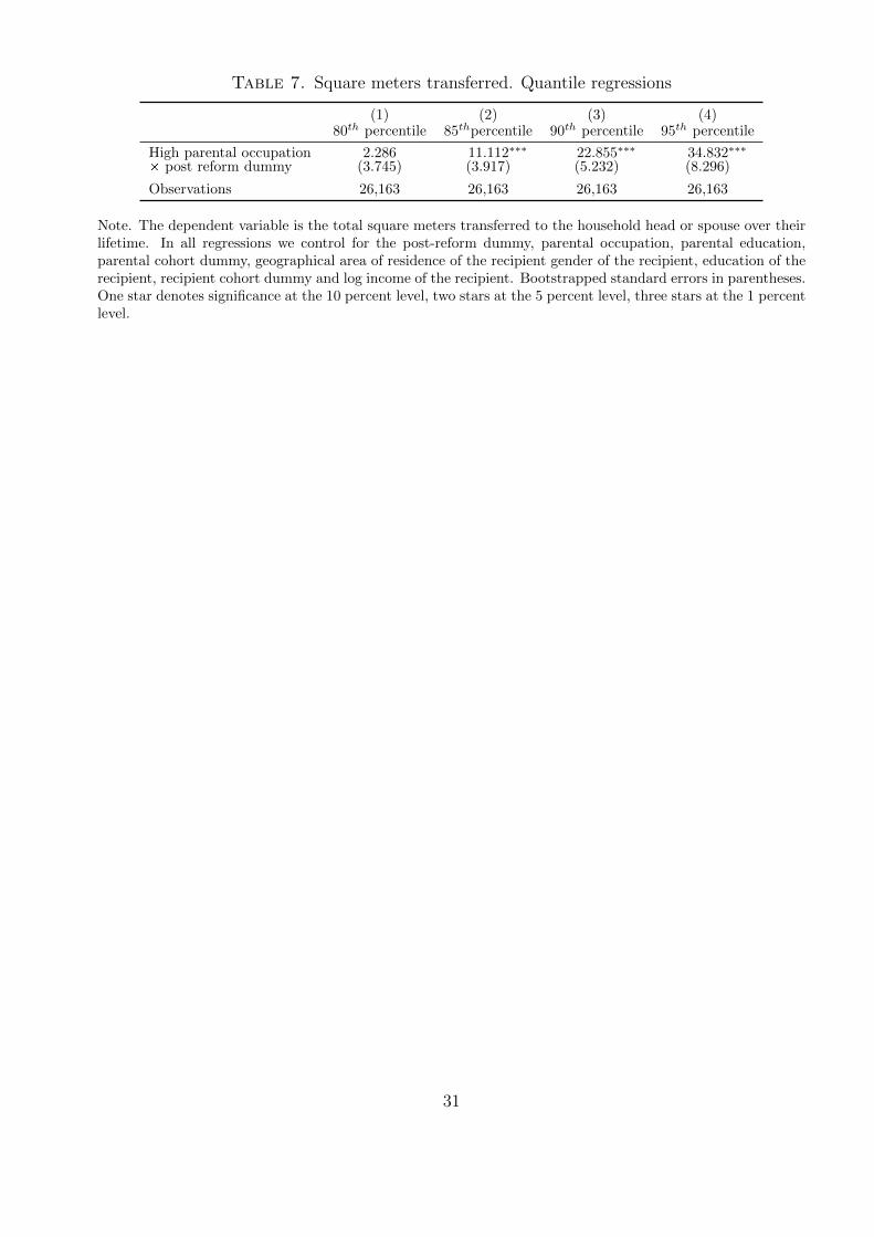
Table 7. Square meters transferred. Quantile regressions
(1) (2) (3) (4)80th percentile 85thpercentile 90th percentile 95th percentile
High parental occupation 2.286 11.112∗∗∗ 22.855∗∗∗ 34.832∗∗∗
Ö post reform dummy (3.745) (3.917) (5.232) (8.296)
Observations 26,163 26,163 26,163 26,163
Note. The dependent variable is the total square meters transferred to the household head or spouse over theirlifetime. In all regressions we control for the post-reform dummy, parental occupation, parental education,parental cohort dummy, geographical area of residence of the recipient gender of the recipient, education of therecipient, recipient cohort dummy and log income of the recipient. Bootstrapped standard errors in parentheses.One star denotes significance at the 10 percent level, two stars at the 5 percent level, three stars at the 1 percentlevel.
31
References
Aigner, D. J. (1973). Regression with a binary independent variable subject to errors of obser-
vation. Journal of Econometrics, 1, 49–60.
Altonji, J. G. ., Hayashi, F., & Kotlikoff, L. J. (1992). Is the extended family altruistically
linked? direct tests using micro data. American Economic Review, 82, 1177–98.
Angrist, J. (2001). Estimation of limited-dependent variable models with binary endogenous
regressors: Simple strategies for empirical practice. Journal of Business and Economic Statis-
tics, 19, 2–16.
Athey, S. & Imbens, G. (2006). Identification and inference in nonlinear difference-in-difference
models. Econometrica, 74(2), 43–497.
Atkinson, A. B. (1971). Capital taxes, the redistribution of wealth and individual savings. The
Review of Economic Studies, 38, 209–227.
Battistin, E. & Sianesi, B. (2011). Misclassified treatment status and treatment effects: An
application to returns to education in the uk. Review of Economics and Statistics, 93(2),
459–509.
Bellettini, G. & Taddei, F. (2009). Real estate prices and the importance of bequest taxation.
Torino: Carlo Alberto Notebooks No. 107.
Bernheim, D. B., Shleifer, A., & Summers, L. H. (1985). The strategic bequest motive. Journal
of Political Economy, 93, 1045–1076.
Bertocchi, G. (2007). The vanishing bequest tax: The comparative evolution of bequest taxation
in historical perspective. IZA Discussion Paper No. 2578.
Blinder, A. S. (1975). Distribution effects and the aggregate consumption function. Journal of
Political Economy, 83, 447–475.
Caballe, J. (1995). Endogenous growth, human capital, and bequests in a life-cycle model.
Oxford Economic Papers, 47, 156–181.
32
Cannari, L. & D’Alessio, G. (2008). Intergenerational transfers in italy. In Household Wealth
in Italy. Bank of Italy.
Carroll, C. D. (2000). Why do the rich save so much? In J. B. Slemrod (Ed.), Does Atlas Shrug?
The Economic Consequences of Taxing the Rich. Harvard University Press and Russell Sage
Foundation, New York.
Chetty, R. (2009). Bounds on Elasticities with Optimization Frictions: A Synthesis of Micro
and Macro Evidence on Labor Supply. Technical report, NBER Working Paper No. 15616.
Gale, W. G. & Perozek, M. G. (2001). Do estate taxes reduce saving? In W. G. Gale, J. R. H.
Jr., & J. B. Slemrod (Eds.), Rethinking Estate and Gift Taxation. Washington: Brookings
Institution Press.
Gale, W. G. & Slemrod, J. B. (2001). Rethinking the estate and gift tax: An overwiev. In
W. G. Gale, J. R. H. Jr., & J. B. Slemrod (Eds.), Rethinking Estate and Gift Taxation.
Washington: Brookings Institution Press.
Gorodnichenko, Y., Martinez-Vazquez, J., & Klara Sabirianova, P. (2009). Myth and reality of
flat tax reform: Micro estimates of tax evasion response and welfare effects in russia. Journal
of Political Economy, 117, 504–554.
Guiso, L. & Jappelli, T. (2002). Private transfers, borrowing constraints and the timing of
homeownership. Journal of Money, Credit and Banking, 34, 315–339.
Holtz-Eakin, D. & Marples, D. (2001). Distortion Costs of Taxing Wealth Accumulation: In-
come Versus Estate Taxes. NBER Working Papers 8261, National Bureau of Economic
Research, Inc.
Hubbard, R. G., Skinner, J., & Zeldes, S. P. (1995). Precautionary saving and social insurance.
Journal of Political Economy, 103(2), 360–99.
Hurd, M. D. (1989). Mortality risk and bequests. Econometrica, 57, 779–813.
Joulfaian, D. (2006). The behavioral response of wealth accumulation to estate taxation: Time
series evidence. National Tax Journal, 59, 253–268.
33
Kopczuk, W. (2009). Economics of estate taxation: A brief review of theory and evidence. Tax
Law Review, 63, 139–157.
Kopczuk, W. & Slemrod, J. (2001). The impact of the estate tax on the wealth accumulation
and avoidance behavior of donors. In W. G. Gale, J. R. H. Jr., & J. B. Slemrod (Eds.),
Rethinking Estate and Gift Taxation. Washington: Brookings Institution Press.
Lewbel, A. (2007). Estimation of average treatment effects with misclassification. Econometrica,
75, 537–551.
Mahajan, A. (2006). Identification and estimation of regression models with misclassification.
Econometrica, 74(3), 631–665.
McDonald, J. F. & Moffit, R. (1980). The uses of tobit analysis. The Review of Economics and
Statistics, 62(2), 318–321.
OECD (2000). Revenue Statistics 1965-1999. Technical report, Paris: OECD.
White, H. (1980). A heteroskedasticity-consistent covariance matrix estimator and a direct test
for heteroskedasticity. Econometrica, 48, 817–838.
Wooldridge, J. M. (2001). Econometric Analysis of Cross Section and Panel Data. Cambridge
(MA): MIT Press.
34
A The effect of taxes on intergenerational transfers
This appendix provides a simple intertemporal consumption model with intergeneration trans-
fers and a tax on transfers. We assume, as in Atkinson (1971) and Blinder (1975), that con-
sumers maximize the following utility function:
U =
∫ T
0
c(t)1−γ
1− γe−ρtdt+ β
b1−δT
1− δe−ρT (3)
where ρ is the discount rate, γ the elasticity of the marginal utility of consumption, δ the
elasticity of the marginal utility of bequests, β the intensity of the bequest motive, T the
length of life and bT bequests net of taxes; furthermore we assume γ > 0, δ > 0, ρ > 0 and
β ≥ 0
The intertemporal budget constraint can be written as:∫ T
0
c(t)e−rtdt+bT
1− τe−rT = W (4)
where r is the interest rate, τ the tax rate on bequests, and W the sum of initial wealth and
the present discounted value of lifetime income. Maximization of equation (3) subject to the
intertemporal budget constraint (4) delivers the following first order conditions:
c(t)−γe−ρt − λe−rt = 0 for all t
βbT e−ρT − λe−rT
1−τ = 0
where λ is the Lagrange multiplier associated with the intertemporal budget constraint. If
δ = γ, we obtain the following expressions for c(t) and bT :
c(t) = c(0)er−ργt (5)
bT = c(0)[β(1− τ)e(r−ρ)T ]1γ (6)
and substituting in the budget constraint we obtain an expression for initial consumption:
c(0) =r − 1
γ(r − ρ)
1− e−[r− 1γ(r−ρ)]T [1− (r − 1
γ(r − ρ))β
1γ (1− τ)
1−γγ ]W (7)
Combining (6) and (7) and it is immediate to check that an increase in the tax rate τ
reduces net bequests, i.e. ∂bT∂τ
< 0
Note that the negative effect of taxes on net bequests applies also if δ 6= γ.
35
B Web Appendix
B.1 Cohort profiles of fraction receiving transfers.
Figure B-1 plots the fraction of households receiving real estate transfers by year-of-birth cohort.
It shows an increase in the fraction for each of the four cohorts after the reform, with the
exception of the fall between 1993 and 1995 for the 40-49 and the 50-59 cohorts. This is not
necessarily a sign of measurement error as, even in a given cohort, the fraction of individuals
declaring to have received real estate transfers may decrease, because part of them may sell
the transfer received. However, Table B-3 shows that excluding year 1993 does not affect our
results, which are, if anything, even larger in magnitude.
B.2 Wealth regressions in the sample of recipients.
Since we do not have wealth data on donors, we focus on the recipients’ wealth distribution, as
discussed in Section 4.1. Table B-1 presents regression of wealth on a dummy equal to 1 if at
least one member of the household is in a high-occupation. Column 1 shows that wealth is 214
thousand euro larger for the high-occupation group. Adding year dummies (column 2) leaves
the results statistically unchanged. Columns 3 and 4 add further controls and show a somewhat
smaller, but still quite significant difference in wealth between high- and the low-occupation
groups.
Table B-2 estimates the probability of wealth being greater than 175 thousand euro. Column
1 reports the baseline specification, where the only control is the high-occupation dummy. The
coefficient is statistically significant and positive, indicating that the probability of being in the
treatment group is just below 25% higher for high-occupation households. The coefficients are
similar across columns, but somewhat lower in column 4 where we control for an extensive list
of variables, including year, education, age, marital status, gender, geographical area, income
and family size.
36

Figure B-1. Fraction of households receiving real estate transfers by cohort
Note. Real estate transfers are defined as bequests or gifts received by the household head or spouse over theirlifetime.
37
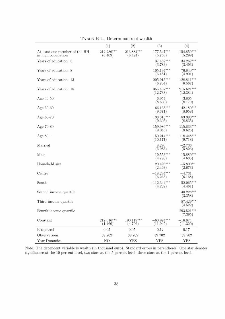
Table B-1. Determinants of wealth
(1) (2) (3) (4)
At least one member of the HH 212.286∗∗∗ 213.884∗∗∗ 177.547∗∗∗ 154.859∗∗∗
in high occupation (6.409) (6.424) (5.756) (5.299)
Years of education: 5 37.482∗∗∗ 34.262∗∗∗
(3.783) (3.493)
Years of education: 8 105.194∗∗∗ 76.840∗∗∗
(5.181) (4.901)
Years of education: 13 205.915∗∗∗ 128.811∗∗∗
(6.704) (6.567)
Years of education: 18 355.437∗∗∗ 215.621∗∗∗
(12.733) (12.384)
Age 40-50 6.954 3.805(8.530) (8.179)
Age 50-60 66.163∗∗∗ 42.180∗∗∗
(9.371) (8.958)
Age 60-70 133.315∗∗∗ 83.393∗∗∗
(9.305) (8.835)
Age 70-80 159.986∗∗∗ 115.833∗∗∗
(9.045) (8.626)
Age 80+ 150.214∗∗∗ 118.448∗∗∗
(10.171) (9.718)
Married 8.290 −2.736(5.983) (5.826)
Male 19.553∗∗∗ 15.880∗∗∗
(4.796) (4.635)
Household size 20.496∗∗∗ −5.800∗∗
(2.493) (2.673)
Centre −18.294∗∗∗ −4.731(6.253) (6.168)
South −112.344∗∗∗ −52.065∗∗∗
(4.252) (4.461)
Second income quartile 40.228∗∗∗
(3.358)
Third income quartile 87.429∗∗∗
(4.522)
Fourth income quartile 293.521∗∗∗
(7.395)
Constant 212.016∗∗∗ 190.119∗∗∗ −60.924∗∗∗ −16.874(1.466) (4.796) (11.942) (11.320)
R-squared 0.05 0.05 0.12 0.17
Observations 39,702 39,702 39,702 39,702
Year Dummies NO YES YES YES
Note. The dependent variable is wealth (in thousand euro). Standard errors in parentheses. One star denotessignificance at the 10 percent level, two stars at the 5 percent level, three stars at the 1 percent level.
38
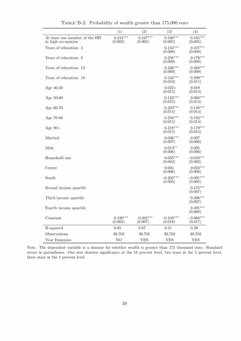
Table B-2. Probability of wealth greater than 175,000 euro
(1) (2) (3) (4)
At least one member of the HH 0.244∗∗∗ 0.247∗∗∗ 0.190∗∗∗ 0.165∗∗∗
in high occupation (0.005) (0.005) (0.005) (0.005)
Years of education: 5 0.134∗∗∗ 0.107∗∗∗
(0.008) (0.008)
Years of education: 8 0.258∗∗∗ 0.179∗∗∗
(0.009) (0.009)
Years of education: 13 0.426∗∗∗ 0.268∗∗∗
(0.009) (0.009)
Years of education: 18 0.542∗∗∗ 0.299∗∗∗
(0.010) (0.011)
Age 40-50 0.027∗ 0.019(0.015) (0.014)
Age 50-60 0.123∗∗∗ 0.086∗∗∗
(0.015) (0.014)
Age 60-70 0.223∗∗∗ 0.148∗∗∗
(0.014) (0.014)
Age 70-80 0.258∗∗∗ 0.192∗∗∗
(0.015) (0.014)
Age 80+ 0.218∗∗∗ 0.179∗∗∗
(0.015) (0.015)
Married 0.036∗∗∗ 0.007(0.007) (0.006)
Male 0.013∗∗ 0.005(0.006) (0.006)
Household size 0.035∗∗∗ −0.010∗∗∗
(0.002) (0.002)
Centre 0.004 0.024∗∗∗
(0.006) (0.006)
South −0.202∗∗∗ −0.091∗∗∗
(0.005) (0.005)
Second income quartile 0.155∗∗∗
(0.007)
Third income quartile 0.306∗∗∗
(0.007)
Fourth income quartile 0.491∗∗∗
(0.008)
Constant 0.430∗∗∗ 0.382∗∗∗ −0.103∗∗∗ −0.068∗∗∗
(0.003) (0.007) (0.018) (0.017)
R-squared 0.05 0.07 0.21 0.29
Observations 39,702 39,702 39,702 39,702
Year Dummies NO YES YES YES
Note. The dependent variable is a dummy for whether wealth is greater than 175 thousand euro. Standarderrors in parentheses. One star denotes significance at the 10 percent level, two stars at the 5 percent level,three stars at the 1 percent level.
39
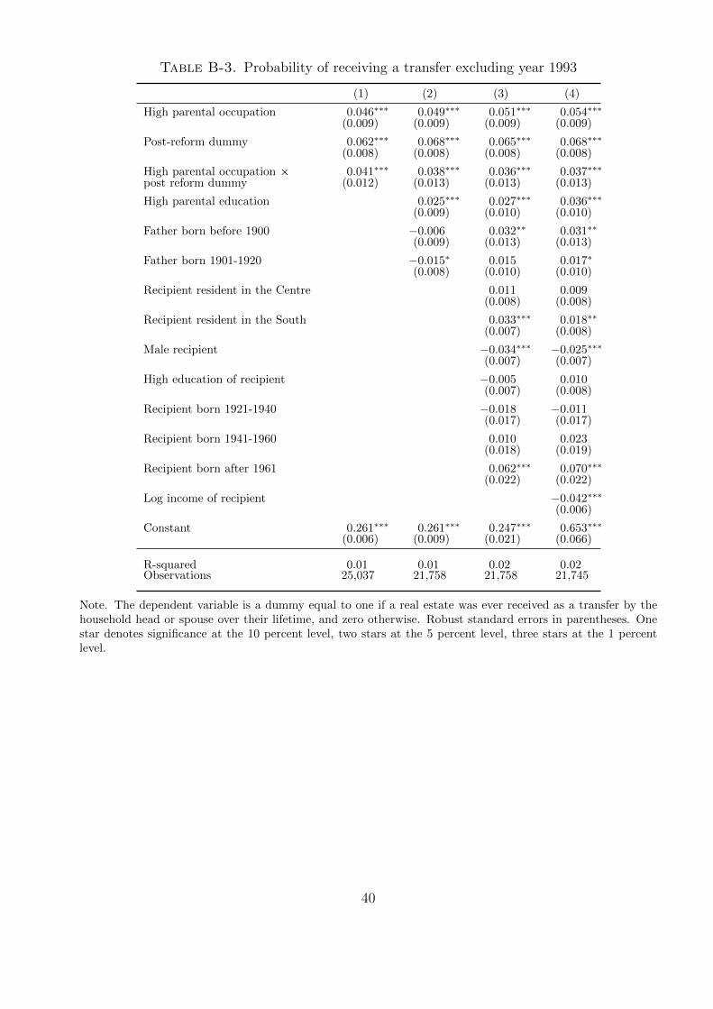
Table B-3. Probability of receiving a transfer excluding year 1993
(1) (2) (3) (4)
High parental occupation 0.046∗∗∗ 0.049∗∗∗ 0.051∗∗∗ 0.054∗∗∗
(0.009) (0.009) (0.009) (0.009)
Post-reform dummy 0.062∗∗∗ 0.068∗∗∗ 0.065∗∗∗ 0.068∗∗∗
(0.008) (0.008) (0.008) (0.008)
High parental occupation Ö 0.041∗∗∗ 0.038∗∗∗ 0.036∗∗∗ 0.037∗∗∗
post reform dummy (0.012) (0.013) (0.013) (0.013)
High parental education 0.025∗∗∗ 0.027∗∗∗ 0.036∗∗∗
(0.009) (0.010) (0.010)
Father born before 1900 −0.006 0.032∗∗ 0.031∗∗
(0.009) (0.013) (0.013)
Father born 1901-1920 −0.015∗ 0.015 0.017∗
(0.008) (0.010) (0.010)
Recipient resident in the Centre 0.011 0.009(0.008) (0.008)
Recipient resident in the South 0.033∗∗∗ 0.018∗∗
(0.007) (0.008)
Male recipient −0.034∗∗∗ −0.025∗∗∗
(0.007) (0.007)
High education of recipient −0.005 0.010(0.007) (0.008)
Recipient born 1921-1940 −0.018 −0.011(0.017) (0.017)
Recipient born 1941-1960 0.010 0.023(0.018) (0.019)
Recipient born after 1961 0.062∗∗∗ 0.070∗∗∗
(0.022) (0.022)
Log income of recipient −0.042∗∗∗
(0.006)
Constant 0.261∗∗∗ 0.261∗∗∗ 0.247∗∗∗ 0.653∗∗∗
(0.006) (0.009) (0.021) (0.066)
R-squared 0.01 0.01 0.02 0.02Observations 25,037 21,758 21,758 21,745
Note. The dependent variable is a dummy equal to one if a real estate was ever received as a transfer by thehousehold head or spouse over their lifetime, and zero otherwise. Robust standard errors in parentheses. Onestar denotes significance at the 10 percent level, two stars at the 5 percent level, three stars at the 1 percentlevel.
40

C The effect of misclassification errors on the estimated
effect of the reform - not for publication
This Appendix discusses how measurement error affects the estimates of the tax reform and
clarifies the assumptions under which the estimates provide a lower bound for the actual effect
of the reform.
C.1 Identification
If the treatment status is correctly measured, the assumption needed for identification is the
following.
Assumption 1 (Mean independence assumption) The average effect of the inheritance tax
removal is given by:
δ ≡ E[Yit|Mi = 1, POSTt = 1]− E[Yit|Mi = 1, POSTt = 0]−
−E[Yit|Mi = 0, POSTt = 1] + E[Yit|Mi = 0, POSTt = 0]
where we assume that:
Yit = α + βMi + γPOSTt + δMi × POSTt + εit
and that:
η11 − η10 − η01 + η00 = 0
where ηrs = E[εit|Mi = r, POSTt = s]
Assumption 1 is standard and is needed to identify δ in all diff-in-diff applications.
Suppose now that an error ridden measure of Mi is available, Mi. Therefore, Mi is subject
to misclassification error. Define:
ν11 = P (Mi = 1|Mi = 1, POSTt = 1)
ν10 = P (Mi = 1|Mi = 1, POSTt = 0)
ν01 = P (Mi = 0|Mi = 0, POSTt = 1)
ν00 = P (Mi = 0|Mi = 0, POSTt = 0)
The νrs are the probabilities of correct classification before and after the reform. From As-
sumption 1 it is easy to show that:
E[Yit|Mi = 1, POSTt = 1] = α + β + γ + δ + η11E[Yit|Mi = 1, POSTt = 0] = α + β + η10E[Yit|Mi = 0, POSTt = 1] = α + γ + η01E[Yit|Mi = 0, POSTt = 0] = α + η00
(8)
41
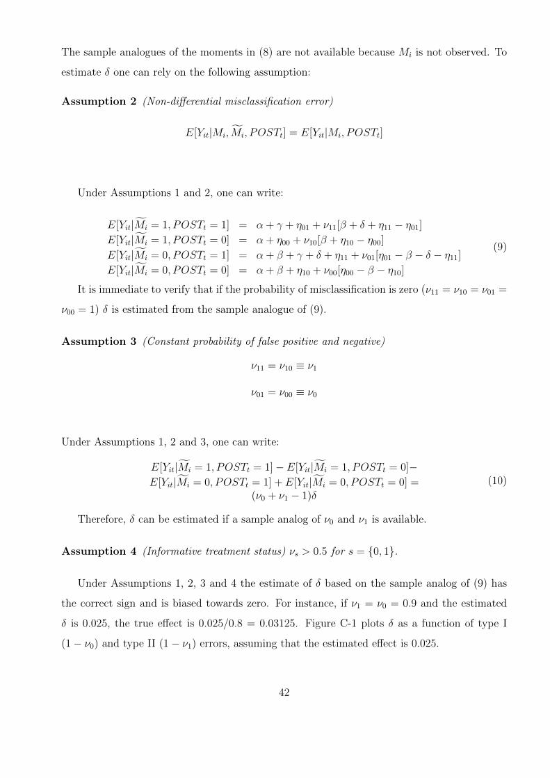
The sample analogues of the moments in (8) are not available because Mi is not observed. To
estimate δ one can rely on the following assumption:
Assumption 2 (Non-differential misclassification error)
E[Yit|Mi, Mi, POSTt] = E[Yit|Mi, POSTt]
Under Assumptions 1 and 2, one can write:
E[Yit|Mi = 1, POSTt = 1] = α + γ + η01 + ν11[β + δ + η11 − η01]E[Yit|Mi = 1, POSTt = 0] = α + η00 + ν10[β + η10 − η00]E[Yit|Mi = 0, POSTt = 1] = α + β + γ + δ + η11 + ν01[η01 − β − δ − η11]E[Yit|Mi = 0, POSTt = 0] = α + β + η10 + ν00[η00 − β − η10]
(9)
It is immediate to verify that if the probability of misclassification is zero (ν11 = ν10 = ν01 =
ν00 = 1) δ is estimated from the sample analogue of (9).
Assumption 3 (Constant probability of false positive and negative)
ν11 = ν10 ≡ ν1
ν01 = ν00 ≡ ν0
Under Assumptions 1, 2 and 3, one can write:
E[Yit|Mi = 1, POSTt = 1]− E[Yit|Mi = 1, POSTt = 0]−E[Yit|Mi = 0, POSTt = 1] + E[Yit|Mi = 0, POSTt = 0] =
(ν0 + ν1 − 1)δ
(10)
Therefore, δ can be estimated if a sample analog of ν0 and ν1 is available.
Assumption 4 (Informative treatment status) νs > 0.5 for s = {0, 1}.
Under Assumptions 1, 2, 3 and 4 the estimate of δ based on the sample analog of (9) has
the correct sign and is biased towards zero. For instance, if ν1 = ν0 = 0.9 and the estimated
δ is 0.025, the true effect is 0.025/0.8 = 0.03125. Figure C-1 plots δ as a function of type I
(1− ν0) and type II (1− ν1) errors, assuming that the estimated effect is 0.025.
42
More generally:
E[Yit|Mi = 1, POSTt = 1]− E[Yit|Mi = 1, POSTt = 0]−E[Yit|Mi = 0, POSTt = 1] + E[Yit|Mi = 0, POSTt = 0] =(ν11 + ν01 − ν10 − ν00)(β + η10 − η00) + (ν11 + ν01 − 1)δ
(11)
Without further restrictions, the data do not provide the sample analogue of (11). Notice,
however, that:ν11 + ν01 = 2− χ1
ν10 + ν00 = 2− χ0
where χ1 ≡ P (Mi = 0|Mi = 1, POSTt = 1) + P (Mi = 1|Mi = 0, POSTt = 1) is the sum of the
probabilities of false positive and false negative values after the reform, and therefore measures
the extent of misclassification after the reform. Similarly, χ0 = P (Mi = 0|Mi = 1, POSTt =
0) + P (Mi = 1|Mi = 0, POSTt = 0) is the sum of the probabilities of false positive and false
negative values before the reform, and measures misclassification before the reform.
A reasonable assumption is therefore the following.
Assumption 5 (Constant probability of misclassification)
χ1 = χ0 ≡ χ
Assumption 5 requires that the probability of misclassification is constant over time. Assump-
tion 5 is weaker than 3, which requires that the probability of false positive and false negative
are constant over time.
Under Assumptions 1, 2 and 5, one can write:
E[Yit|Mi = 1, POSTt = 1]− E[Yit|Mi = 1, POSTt = 0]−E[Yit|Mi = 0, POSTt = 1] + E[Yit|Mi = 0, POSTt = 0] =
(1− χ)δ
Therefore, δ can be estimated provided that the sample analog of χ can be found. Notice that
the sample analogues of ν11, ν10, ν01, and ν00 can be used to test Assumptions 3 and 5.
Under Assumption 4, 1− χ < 1 and the usual attenuation bias result applies.
We consider in turn two alternative identification assumptions. First, we change before and
after the reform.
43
Assumption 6 (Only false positive occur with constant probability)
ν01 = ν00 = 1
ν11 − ν10 = 0
Under Assumptions 1, 2 and 6, one can write:
E[Yit|Mi = 1, POSTt = 1]− E[Yit|Mi = 1, POSTt = 0]−E[Yit|Mi = 0, POSTt = 1] + E[Yit|Mi = 0, POSTt = 0] = ν11δ
(12)
The sample provides the analog of the left-hand side of (12), which is a downward biased
estimate of δ, since ν11 is smaller than one. Notice that if an estimate for ν11 can be found,
also δ can be estimated.
Second, we assume that only false negative occur with a probability that does not change
before and after the reform.
Assumption 7 (Only false negative occur with constant probability)
ν11 = ν10 = 1
ν01 − ν00 = 0
Under assumptions 1, 2 and 7, one can write:
E[Yit|Mi = 1, POSTt = 1]− E[Yit|Mi = 1, POSTt = 0]−E[Yit|Mi = 0, POSTt = 1] + E[Yit|Mi = 0, POSTt = 0] = ν01δ
(13)
The data provide the sample analog of the left-hand side of (13) and δ can be estimated if
an estimate for ν01 is available. Since ν01 is smaller than one, the sample analog of left-hand
side of (13) is a downward biased estimate of δ.
We now show how to bound δ when Yit is a zero left-censored variable:
Yit =
{Y ∗it if Y ∗
it ≥ 00 otherwise
where:
Y ∗it = α + βMi + γPOSTt + δMi × POSTt + εit
We further assume that εit is normal with mean zero and standard deviation σ,
E(Yit|Y ∗it > 0,Mi, POSTt) = α + βMi + γPOSTt + δMi × POSTt+
λ(−α+βMi+γPOSTt+δMi×POSTtσ
)(14)
44

where:λ(−α+βMi+γPOSTt+δMi×POSTt
σ) =
φ(−α+βMi+γPOSTt+δMi×POSTtσ
)/Φ(−α+βMi+γPOSTt+δMi×POSTtσ
)
and φ(·) and Φ(·) are the standard Gaussian pdf and cdf, respectively.
Under Assumption 2, we can write:
E[Yit|Y ∗it > 0, Mi = 1, POSTt = 1] = α + γ + λ01 + ν11[β + δ + λ11 − λ01]
E[Yit|Y ∗it > 0, Mi = 1, POSTt = 0] = α + λ00 + ν10[β + λ10 − λ00]
E[Yit|Y ∗it > 0, Mi = 0, POSTt = 1] = α + β + γ + δ + λ11 + ν01[λ01 − β − δ − λ11]
E[Yit|Y ∗it > 0, Mi = 0, POSTt = 0] = α + β + λ10 + ν00[λ00 − β − λ10]
(15)
where:λ11 ≡ λ(−α+β+γ+δ
σ)
λ01 ≡ λ(−α+γσ
)
λ10 ≡ λ(−α+βσ
)λ00 ≡ λ(−α
σ)
Notice that the assumption that εit is normal with mean zero and standard deviation σ is made
for convenience, but it is not restrictive for the derivation of (15), which would be unchanged
if we interpret λrs as E(εit|εit > −(α + βr + γs+ δr × s)), where r = {0, 1} and s = {0, 1}.
If ν11 = ν10 = ν01 = ν00 = 1, the diff-in-diff parameter is:
E[Yit|Y ∗it > 0, Mi = 1, POSTt = 1]− E[Yit|Y ∗
it > 0, Mi = 1, POSTt = 0]−E[Yit|Y ∗
it > 0, Mi = 0, POSTt = 1]− E[Yit|Y ∗it > 0, Mi = 0, POSTt = 0] =
δ + λ11 − λ10 − λ01 + λ00 ≡ δ
The sample provides the analog of the following population quantity:
E[Yit|Y ∗it > 0, Mi = 1, POSTt = 1]− E[Yit|Y ∗
it > 0, Mi = 1, POSTt = 0]−E[Yit|Y ∗
it > 0, Mi = 0, POSTt = 1] + E[Yit|Y ∗it > 0, Mi = 0, POSTt = 0] =
(ν11 + ν01 − ν10 − ν00)(β + λ10 − λ00) + (ν11 + ν01 − 1)δ
(16)
Under Assumptions 3, (16) becomes:
(ν1 + ν0 − 1)δ
which under Assumption 4 implies that the estimated δ is a lower bound for the actual diff-in-
diff parameter.
C.2 Estimation
If the sample analog of the probabilities of correct classification were known, it would be im-
mediate to estimate the effect of the tax reform and the misclassification bias, which, under
45
Assumption 3 or 5, 6, 7 is the same, regardless of whether the left-hand-side variable is continu-
ous, binary or zero left-censored. However, we don’t observe the wealth distribution of donors,
and therefore have no direct evidence on the probabilities of correct classification.
To gain insights on the wealth distribution of donors, we focus on the wealth distribution of
recipients. If the ranks are invariant between the two distributions, it would be immaterial to
estimate the probability of correct classification with one of the two. While in the short time
span of our data the GINI index of household wealth is roughly constant at 61-62%, over long
periods of time the rank invariance assumption is unlikely to hold if the wealth distribution
changes from one generation to the next.
Let’s assume that the probabilities of correct classification don’t change after the reform
and call νD0 and νD1 the sample analogs of ν0 and ν1 in the wealth distribution of donors in
the control and in the treatment group, respectively. In our data νD0 and νD1 are not directly
observable. However, we observe their counterparts in the distribution of recipients, νR0 and
νR1 . Under rank invariance, νD0 = νR0 and νD1 = νR1 . More generally, if the rank invariance does
not hold, we assume that:νR0 = νD0 + ξ0νR1 = νD1 + ξ1
where ξ0 and ξ1 are the slippages from rank invariance.
If we had information on the slippages, the sample analog of (10) would be:
[νR0 + νR1 − (ξ0 + ξ1)− 1]δ (17)
which, however, is not operational in our setting since we do not have information on (ξ0 + ξ1).
To make (17) operational we make the following assumption:
Assumption 8 (Slippages from rank invariance)
ξ0 ∈ [νR0 − 1, νR0 − 0.5]
ξ1 ∈ [νR1 − 1, νR1 − 0.5]
Assumption 8 implies that νD0 and νD1 are larger than 0.5. The assumption is the analog of
Assumption 4, and provides the basis to compute the true effect of the reform, which is done
in four steps:
46
1. We estimate the model to get δ, the estimated effect of the reform.
2. We estimate νR0 and νR1 from the wealth distribution of the recipients.
3. We draw the sequence{ξ0,m
}1000
m=1(and
{ξ1,m
}1000
m=1) from a uniform distribution with lower
bound equal to νR0 − 1 (νR1 ) and upper bound equal to νR0 − 0.5 (νR1 − 0.5 ), as required
by assumption 8.32
4. We compute the true effect of the reform as: δ = δ1000
∑1000m=1
1
(νR0 +νR1 −(ξ0,m+ξ1,m)−1)
Figure C-1. True effect as a function of type I and II errors
Note. The figure shows the true effect as a function of the type I (1− ν0) and type II (1− ν1) errors assumingthat the estimated effect is 0.025.
32Lacking information on the slippages distribution, we prefer to use a flat prior, such as the uniform. Ex-perimenting with beta distributions produces similar results.
47
D Marginal effects
We explain below how we compute the marginal effect of the reform on square meters trans-
ferred, which is left-censored:
Yit =
{Y ∗it if Y ∗
it ≥ 00 otherwise
We assume that :
Y ∗it = α + βMi + γPOSTt + δMi × POSTt + εit
where Mi and POSTt are, respectively, the treatment group and the post-reform dummies.
The effect of the reform on Y ∗it is δ under the assumption that:
η11 − η10 − η01 + η00 = 0
where ηrs = E[εit|M∗i = r, POSTt = s]. The parameter δ measures the difference between the
change in Y ∗it between the treatment and the control group.
In addition to the effect on Y ∗it , we can compute the effect of the reform on E(Yit|Y ∗
it ≥
0,Mi, POSTt) (the conditional mean), on Pr(Y ∗it ≥ 0|Mi, POSTt), and on E(Yit|Mi, POSTt)
(the unconditional mean). If we assume that εit is normal with mean zero and standard
deviation σ, the conditional mean square meters transferred is:
E(Yit|Y ∗it > 0,Mi, POSTt) = α + βMi + γPOSTt + δMi × POSTt+
λ(−α+βMi+γPOSTt+δMi×POSTtσ
)(18)
where:λ(−α+βMi+γPOSTt+δMi×POSTt
σ) =
φ(−α+βMi+γPOSTt+δMi×POSTtσ
)/Φ(−α+βMi+γPOSTt+δMi×POSTtσ
)
and φ(·) and Φ(·) are the standard Gaussian pdf and cdf, respectively.
The effect of the tax reform on E(Yit|Y ∗it > 0,Mi, POSTt) is therefore:
E(Yit|Y ∗it > 0,Mi = 1, POSTt = 1)− E(Yit|Y ∗
it > 0,Mi = 1, POSTt = 0)−E(Yit|Y ∗
it > 0,Mi = 0, POSTt = 1) + E(Yit|Y ∗it > 0,Mi = 0, POSTt = 0) =
δ + λ(−α+β+γ+δσ
)− λ(−α+βσ
)− λ(−α+γσ
) + λ(−ασ)
The effect of the tax reform on Pr(Y ∗it ≥ 0|Mi, POSTt) is:
Φ(−α+β+γ+δσ
)− Φ(−α+βσ
)− Φ(−α+γσ
) + Φ(−ασ)
To compute the effect on the unconditional mean of Yit notice that one can write:
E(Yit|Mi, POSTt) = E(Yit|Y ∗it > 0,Mi, POSTt)× Pr(Y ∗
it ≥ 0|Mi, POSTt)
48
which implies that the effect of the tax reform on E(Yit|Mi, POSTt) can be obtained as:
E(Yit|Mi = 1, POSTt = 1)− E(Yit|Mi = 1, POSTt = 0)−−E(Yit|Mi = 0, POSTt = 1) + E(Yit|Mi = 0, POSTt = 0) =
α[Φ(−α+β+γ+δ
σ)− Φ(−α+β
σ)− Φ(−α+γ
σ) + Φ(−α
σ)]
+
+β[Φ(−α+β+γ+δσ
)− Φ(−α+βσ
)] + γ[Φ(−α+β+γ+δσ
)− Φ(−α+γσ
)] + δΦ(−α+β+γ+δσ
)+
φ(−α+β+γ+δσ
)− φ(−α+βσ
)− φ(−α+γσ
) + φ(−ασ)
The marginal effects are estimated replacing α, β, γ, δ and σ with their maximum likelihood
estimates. Standard errors are obtained from non-parametric bootstrap.
E The counterfactual distribution of square meters trans-
ferred in the treatment group
This section shows how we obtain the counterfactual distribution of the square meters trans-
ferred in the treatment group. We call Y10 square meters transferred in the treatment group
before the reform. The q quantile of the distribution of Y10 is defined by q = FY10(y). Using
the standard potential outcome notation, Y 011 are square meters transferred in the treatment
group after the reform, had the reform not happened.
To obtain the counterfactual value at the q quantile, we first define:
∆QDID = F−1Y01
(q)− F−1Y00
(q) = F−1Y01
(FY10(y))− F−1Y00
(FY10(y))
which is the difference in the outcome in the control group before and after the reform. The
counterfactual value at the the q quantile is obtained by adding ∆QDID to y:
kQDID(y) = y + ∆QDID
Repeating this procedure for each q-quantile of the distribution of Y10, we obtain the counter-
factual distribution of square meters transferred in the treatment group.
49