1

YOUNG LIVES STUDENT PAPER

Do Households’ Water and Sanitation Choices Really Matter for Child Health?

Martina Kirchberger

August 2008

Paper submitted in part fulfilment of the requirements for the degree of MSc in Economics for Development at the University of Oxford.

The data used in this paper comes from Young Lives, a longitudinal study investigating the changing nature of childhood poverty in Ethiopia, India (Andhra Pradesh), Peru and Vietnam over 15 years. For further details, visit: www.younglives.org.uk

Young Lives is core-funded by the Department for International Development (DFID), with sub-studies funded by IDRC (in Ethiopia), UNICEF (India), the Bernard van Leer Foundation (in India and Peru), and Irish Aid (in Vietnam).

The views expressed here are those of the author. They are not necessarily those of the Young Lives project, the University of Oxford, DFID or other funders.

2

Do households’ water and sanitation choices really matter for child health?

Martina Kirchberger University of Oxford

August 2008

3

Acknowledgements

I would like to express my sincere thanks to Stefan Dercon for the guidance, feedback and encouragement he has provided. I would also like to thank Francis Teal, Ingo Outes-Leon, Jaleel Partow and Chris Cormency for helpful comments.

4

Abstract

This paper investigates the impact of usage patterns of water and sanitation on the health of children in Ethiopia, once supply side factors are controlled for. A comprehensive set of controls is employed to account for individual heterogeneity driven by time-invariant unobservables, time-invariant and time-variant observables. The results from the pooled cross-section estimated by OLS suggest that there is a strong relationship between water and sanitation choices of a household and a child’s weight-for-age z-scores. This correlation disappears when unobserved time-invariant fixed effects are removed through a fixed effects specification. However, the fixed effects model reveals that children from the poorest families who improved usage patterns of water and sanitation exhibited a significantly larger growth in weight-for-age z-scores between the two periods. The effect remains robust across a number of different specifications, including a dynamic model to allow for catch-up effects and an instrumented version of a dynamic model. Consequently, the effectiveness of investments in water and sanitation infrastructure can be leveraged by influencing the choices made by households regarding the type of water and sanitation.

5

Contents

1.  Introduction ................................................................................................................................ 6 

2.  Literature Review....................................................................................................................... 7 

3.  Model ......................................................................................................................................... 9 

4.  Data .......................................................................................................................................... 15 

5.  Results ...................................................................................................................................... 19 

6.  Conclusion................................................................................................................................ 26 

7.  Bibliography............................................................................................................................. 28 

8.  Annex ....................................................................................................................................... 33 

6

Introduction

Approximately 50% of under five deaths worldwide are associated with undernutrition (Pelletier 1995; Caulfield 2004). Undernourished children suffer from delayed cognitive development and perform worse in school (Pollitt et al. 1993; Behrman 1996). Moreover, lower height resulting from chronic undernutrition is associated with lower lifetime earnings (Strauss and Thomas 1998), trapping children from poor families in poverty. Malnutrition is primarily a function of nutritional intake, disease incidence and environmental factors such as use of safe water and clean sanitation, access to health facilities and the disease environment. Given that catch-up of growth for children is observed to take place mainly before the age of three (Martorell et al. 1994), the impact of access to water and sanitation during childhood can have life-long consequences1. This essay investigates how household demand for clean water and sanitation impacts a child’s growth path, measured by changes in height-for-age and weight-for-age. Clean water and sanitation could impact child health through three major pathways (Burger and Esrey 1995). First, they decrease exposure to pathogens, thereby reducing diarrhoea and other diseases such as ascariasis, guinea worm, schistosomiasis and trachoma. Second, domestic access to water reduces time and energy allocated to fetching water that can be redirected towards food preparation, income-generating activities or health-promoting activities. Since fetching water is primarily performed by females in a household, easier access to clean water can have strong beneficial effects for children. Third, decreased exposure to pathogens of a child’s parents reduces incidence and duration of illness, improving productivity and thereby raising household income, a major determinant of child welfare. However, if parents substitute other inputs into the health production function such as food when household health infrastructure improves, then the effect of water and sanitation could be insignificant or even negative. The data used in this study cover the period 2002-7 in Ethiopia. This period is characterised by a rapidly changing environment in which GDP per capita growth picked up and averaged 11% (World Bank 2008a), and there was substantial investment in water and sanitation infrastructure, allowing households to switch to safer sources. Large variation in usage patterns across time thus make it very suitable to study the impact of levels and changes in households’ water and sanitation choices on child health. The contribution of this paper is threefold: (i) while most of the empirical evidence focuses on evaluating the impact of changes in access to water and sanitation facilities on child health, this paper takes a different view by investigating the impact of households’ usage patterns of water and sanitation on child health after controlling for time-invariant and time-variant supply side factors, such as investments in water and sanitation infrastructure; (ii) the use of a panel dataset for 1500 children in Ethiopia which reveals variations in the type of water and sanitation usage across space and time 1 Catch-up is defined in line with Payne (1993) as a period of accelerated growth following a period of nutritional deprivation or illness, allowing a child to partially of even fully offset growth deficits.

7

allows to control for unobserved time-invariant individual and household characteristics; (iii) endogeneity concerns in estimating child growth equations relating to dynamic modelling, omitted variables and unobserved heterogeneity are systematically addressed and advantages as well as disadvantages of different specifications are evaluated. The obtained results from the pooled cross-section estimated by OLS suggest that there is a strong homogenous correlation between water and sanitation choices of a household and child health. This correlation disappears when unobserved time-invariant fixed effects are removed through a fixed effects specification. However, the model reveals that children from the poorest families who shifted to improved water and sanitation usage patterns exhibited a significantly larger growth between the two periods. The effect remains robust to a number of different specifications, including a dynamic model (to allow for catch-up effects) and an instrumented version of a dynamic model. These findings have strong implications for policy-making. They highlight the importance of households’ demand for water and sanitation; in particular, this study shows that households can leverage the effectiveness of investments in water and sanitation infrastructure by deciding to switch to an improved source of water and type of sanitation. Furthermore, the improvement in health outcomes is highest for children from the poorest families. Influencing households’ water and sanitation choices has therefore the potential to bring the greatest benefits to children of most deprived families. In order to exploit these additional benefits, more research on the determinants of households’ water and sanitation choices is needed. Constraints related to the use of a safe source of water include the distance to the nearest source of water, transport options and the quantity of water available, which determine the price of clean water to the household. Cultural factors and tradition play an important role in the use of better sanitation (Ayele, 2005). Collecting data on these variables would shed further light on context-specific underlying constraints households face and help design programmes that take these into account. This would also entail research on the most effective communication strategies to increase households’ awareness and engagement to choose a safe source of water and clean sanitation. The paper is structured as follows: the next section briefly discusses the literature; section three lays out the empirical specification and discusses econometric issues; section four describes the data and section five presents the results; the last section concludes.

Literature Review

The impact of access to water and sanitation facilities on child health has been researched in a large number of studies producing mixed results ranging from positive to insignificant to negative relationships2. The methodologies employed can be roughly

2 The most commonly used dependent variables are mortality, prevalence and duration of diarrhoea, diseases such as ascariasis (roundworm), dracunculiasis (guinea worm), hookworm infection, schistosomiasis and trachoma, and anthropometric measures. Since this paper uses anthropometric measures as dependent variables, the literature review is limited to studies investigating anthropometrics.

8

divided into two strands: (i) those which estimate quasi-reduced form health demand functions including households’ own access to water and sanitation as an explanatory variable; and (ii) studies which estimate strict reduced form health demand equations and therefore treat water and sanitation as endogenous household choices and only include means or non-self means of access to safe water and sanitation at the community level. Lee et al. (1997) estimate the impact of better nutrition, and a household’s water quality and sanitation on child health for panel datasets for the Philippines and Bangladesh, considering changes in resource allocation to health linked to better infrastructure as inputs in the health production function. They find that the positive effect of improved water and sanitation is underestimated in reduced form equation models due to reduced allocation of household resources to health as water and sanitation facilities improve. Merchant et al. (2003) observe that children stunted at baseline had a 17% higher chance of reversing stunting 18 months later if they were from homes with water and sanitation compared to children coming from homes which did not have either. Esrey (1996) illustrates with cross-sections from Burundi, Ghana, Togo, Uganda, Sri Lanka, Morocco, Bolivia and Guatemala that children with improved water and sanitation were taller and heavier. Further, the benefit of water was only present when sanitation was improved and the best source of water present, a result in line with Checkley et al. (2004). Esrey and Habicht (1988) find that the effect of improved sanitation on mortality rates for Malaysian children was biggest if the mother was illiterate, but with the opposite effect for the case of improved water. Esrey et al. (1992) find the biggest effect on weight and height of children when households have both clean sanitation and increased volume of water during the wet season. The positive health effect of clean water and sanitation disappears for children in Eritrea when including controls for socio-economic factors (Woldemicael 2000). Strauss (1990) finds from a cross-section of 504 children from rural Côte d’Ivoire using household random effects that children from villages whose dominant source of water are wells without pumps have significantly lower height-for-age and weight-for-age z-scores compared to children from villages which get their water from wells with pumps or private taps. However, children from villages which predominantly use natural sources of water, i.e. rainfall, rivers or lakes do not have a significantly different height-for-age nor weight-for-age z-score. Thomas and Strauss (1992) show that the number of water installations per 1000 population is negatively associated with height-for-age for children in rural Brazil but positively associated with height-for-age for children in urban Brazil. Gragnolati (1999) also finds an ambiguous effect for children in Guatemala. While the proportion of households in a community with piped water connections is positively associated with height-for-age, the proportion of households with flush toilets is negatively associated with height-for-age. A study using data from the Philippines suggests that the effect of water depends on the age of the child (Barrera 1990). The prevalent source of water in the community is insignificant for the whole sample, but positively associated with height-for-age for 0-2 month old children. However, the prevalent type of toilet in the community is negatively associated with height-for-age for 0-2 month old children. When adding interaction terms he finds that For an overview of studies using other outcome variables see Hoddinott (1997) or for a more recent study on prevalence and duration of diarrhoea see Jalan and Ravallion (2003).

9

water and education are substitutes, while sanitation and education are complements. There are two studies which find unambiguously positive effects. Lavy et al. (1996) conclude from their analysis of a cross-section of Ghanaian children that children living in rural areas with poor sanitation are significantly worse off both in terms of height-for-age and weight-for-age. Further, Alderman et al. (2003) investigate the impact of household’s own access to water and sanitation as well as externalities by using non-self cluster means. Their results suggest that while the positive effect of households’ own access to water and sanitation vanishes when they control for the non-self cluster means, there are significant externalities associated with investments by neighbouring households in water and sanitation. The large variation in results reported in these various studies can be explained by a number of factors relating to unobserved heterogeneity, which is discussed in depth in the next section of this paper. Although three of the above mentioned studies (Merchant et al. 2003; Checkley 2004; Esrey et al. 1992) employ longitudinal datasets, none of these studies observe changes in the type of water and sanitation used by the household. In this context, it is not possible to account for individual and household fixed effects, as this would eliminate the time-invariant variable of interest. Therefore, similarly to OLS estimates obtained in most studies, these estimates risk being severely biased due to the presence of unobserved individual and household characteristics. These include preferences, behavioural changes within households, political connections of a community, cultural and traditional beliefs, contamination of ground water, disease environment and health awareness. Another reason for biased OLS results is the endogenous placement of water and sanitation infrastructure (Rosenzweig and Wolpin 1986). If, for instance, newly constructed wells and sanitation facilities are concentrated in areas with the highest rates of malnutrition, cross-sectional data will find a positive correlation between improved water and sanitation and undernutrition.

Model

This section starts by outlining a theoretical model, from which a reduced form health demand function and a number of different econometric specifications are derived. Econometric issues including strengths and weaknesses of the different models are discussed. The specifications range from a pooled OLS estimation to a fixed effects specification, a conditional growth model, and finally a conditional growth model with instruments for the lagged dependent variable. Households maximize a utility function of the form

U=U(Hi, Zi, Li) (1)

where Hi represents the health of household member i, Zi the consumption of goods and services and Li leisure, subject to a budget and a time constraint. This maximization yields the following reduced form health demand function (Behrman and Deolalikar 1988; Pitt 1993):

Hict = H(pct, Xict, ai, ah, ac, uict) (2)

10

where health Hict of child i in community c at time t depends on food prices pct, on observable exogenous individual and household characteristics Xict such as age, gender, whether the household head is a parent of the child, whether the caretaker is the household head, highest education attained by caretaker, unobservable individual, household and community characteristics, and a random error term uict. Inputs into the health production function are nutrients, water and sanitation conditions, health-related inputs such as medical care utilization and mothers schooling, age, household characteristics, community endowments and endowments of the mother. The inclusion of water and sanitation in H therefore yields a quasi-reduced form health demand function (Behrman and Deolalikar 1988). Height-for-age and weight-for-age z-scores are used as proxies for child health. These anthropometric indicators are calculated by subtracting the median height (weight) of a reference population from a child’s height (weight) and dividing by the standard deviation3 (WHO 1995). Children whose height-for-age (weight-for-age) z-score is less than two standard deviations below the median are classified as stunted (underweight). Height-for-age reflects long-run nutritional deprivation, poor economic conditions and chronic or repeated diseases. Weight-for-age is a composite indicator capturing aspects of stunting as well as wasting (low weight-for-height). Weight-for-height is available only for children up to 60 months old. Thus, although desirable, it could not be used in this analysis as the exclusion of children older than 60 months would have halved the sample. The main estimated equation of interest is:

z-scoreict = β0 + δ0 timet + β′ WS WSict + β′X Xict + vict (3)

where vict = ai + ah + ac + uict. The z-score of child i in cluster c at time t is a function of timet

4, a vector indicating the type of water and sanitation used by the household WSict, a vector of time-varying as well as time-invariant exogenous child and household characteristics Xict, and a composite error term vict containing a time invariant child fixed effect5 ai (eg. genetic endowments), time-invariant unobservables at the household level ah (eg. parents preferences), a cluster effect ac (eg. disease environment, food prices) and an idiosyncratic error uict

6; δ0, β′WS, and β′X are the parameters to be estimated. Pooled OLS will give consistent and unbiased parameter estimates if E(vict| Xict, WSict ) = 0. If the child, household, or cluster effects are correlated with the explanatory variables in WSict or Xict, so that E(ai, h, c| Xict, WSict) ≠ E(ai, h, c) then pooled OLS yields biased and inconsistent estimates. For example, some parents might put a higher weight on child health in their utility function and, thus, invest in better water and sanitation facilities. However, since we do not have a measure of how much parents care about their 3 The indicators have been calculated using the 2006 WHO Child Growth Standards for children aged 0-60 months (WHO 2007) and the WHO Reference 2007 for children who were older than 60 months in round two (De Onis et al. 2007). 4 The panel dataset used in this paper has two time periods, so that timet can be interpreted as a time trend or equally a dummy variable which is equal to one in t, and 0 in t-1. 5 Given the large number of random draws from the population it makes sense to treat ai as a random variable (Wooldridge 2002). 6 It is assumed here that there is only one child per family, so that individual and household fixed effects represent identical transformations. Section 4 describes the data in detail.

11

children, this is contained in the residual, ah, which is correlated with the regressors. If the estimates then suggest that water and sanitation facilities benefit child health, the estimate could be biased upward as it simply picks up how much parents care for their children, but not the partial effect of improved water and sanitation on child health. Differencing equation (3) yields

∆z-scoreict= δ0+ β′ WS ∆WSict + β′X ∆Xict + ∆uict (4) In a two-period panel, first differences are computationally equivalent to individual and household fixed effects. Since there is only one child per family, both the time-invariant child fixed effect ai and the household fixed effect ah are eliminated by differencing or time-demeaning the data. Further, time-invariant unobservables at the cluster level are removed as well through this transformation. If there are no time-variant unobservables correlated with the regressors, equation (4) yields unbiased and consistent estimates. Nevertheless, the fixed effects estimator has several shortfalls. The differencing procedure eliminates approximately half of the observations resulting in a loss of efficiency, and this loss is proportionately highest with a two time period panel (Deaton 1997). Furthermore, an underlying assumption is that time-invariant variables have no effect on growth, as is it evident from above that any time-invariant variables contained in Xict drop out when differencing the data. However, the latter concern can be addressed by including time dummy variables, a vector of time-invariant variables Cic and their interaction terms in the levels equation. This allows the impact of time-invariant variables to differ across time periods. Including time dummy variables, time-invariant observables as well as their interaction terms yields

z-scoreict = β0 + δ0 timet + β ′C Cic + timet β ′C Cic + β′ WS WSict + β′X Xict + vict (5)

where vict = ai + ah + ac + uict and where Cic represents a vector of time-invariant characteristics, such as community, gender of the child and mother’s height. Differencing (5) gives

∆z-scoreict = δ0 + β ′C Cic + β′ WS ∆WSict + β′X ∆Xict + ∆uict (6). Equation (6) not only removes time-invariant unobservables, as equation (4), but additionally controls for the effect of time-invariant observables on changes in the z-score over time compared to the base period. In a last extension of this model, for the research question this paper asks, it is of additional interest to control for the impact of exogenous initial conditions on changes over time. Expanding equation (5) with interaction terms of time dummy variables and baseline variables gives

z-scoreict = β0 + δ0 timet + β ′C Cic + timet β ′C Cic + β ′V Vict-1 + timet β ′V Vict-1 + β′ WS WSict

+ β′X Xict + vict (7)

where vict = ai + ah + ac + uict

12

and differencing yields

∆z-scoreict = δ0 + β ′′C Cic + β ′V Vict-1 + β′ WS ∆WSict + β′X ∆Xict + ∆uict (8).

This transformation eliminates time-invariant unobservables ai, ah, ac and controls for differences in partial effects of time-invariant observables compared to the base period in addition to differences in partial effects of initial conditions. Out of the above outlined models, the empirical part presents results for the pooled OLS (3), first differences (4), first differences controlling for time-invariant variables (6) and first differences controlling for time-invariant variables as well as initial conditions (8). Given the cumulative growth process of children, it is reasonable to expect that current growth not only depends on changes in time-variant variables, time-constant variables, and past exogenous factors, but health is a dynamic process in that past growth is an important variable impacting current growth (Strauss and Thomas 2008). In this context, several authors have used frameworks that start from households maximizing an intertemporal utility function with certain desirable properties such as inter-temporally additive preferences, and individual sub-utility functions increasing and quasi-concave in their arguments (Foster 1995; Hoddinott and Kinsey 2001). The utility maximization subject to a budget constraint in each period, a health production function that incorporates dynamic effects, and expected future wages of children yields the following reduced form health demand equation

Hict = H(Hict-1, Hict-2, Hict-3,..., Hict-S, pct, Xict, ai, ah, ac, uict) (9)

s = 1, 2, 3,..., S

where health of child i in cluster c at time t depends on health in all previous periods up to birth where s=S. Assuming that past health status equally impacts health in the current period for all t, one possible econometric representation for t and t-1 could be (for simplicity the time-invariant and time-variant controls as well as their interaction effects with time are omitted here):

z-scoreict = β0 + δ0 timet + β′ Z + β′ WS WSict + β′X Xict + vict (10)

where vict= ai + ah + ac + uict and

z-scoreict-1 = β0 + δ0 timet-1 + β′ Z + β′ WS WSict-1 + β′X Xict-1 + vict-1 (11)

where vict-1=ai + ah + ac + uict-1

Subtracting (11) from (10) translates into a dynamic conditional demand child growth equation, which is a special form of equation (8), including the initial z-score in the vector of time-variant controls

13

∆z-scoreict = δ0 + βZ z-scoreict-1 + β′ WS ∆WSict + β′X ∆Xict + ∆uict (12)

Equation (12) investigates the impact of ∆WSict and ∆Xict on child growth, conditional on initial height or weight. To derive unbiased estimators for equation (12) we require E(∆uict| z-scoreict-1, ∆WSict, ∆X ict)=0, which is violated by construction since (11) illustrates that z-scoreict-1 contains uict-1 which is part of the residual in (12). However, equation (12) has the advantage of removing the time-invariant individual, household and community fixed effects ai, ah and ac, so that only ∆uict is left as the residual. Therefore, the bias, which was due to correlation between the fixed effects and the water and sanitation variables in levels, has been removed. As this paper is particularly interested in the impact of water and sanitation use, this is important in reducing the bias on these coefficients. It is important to point out that the coefficients βZ, β′ WS, and β′X represent the short run impacts, while the long run impacts, denoted by stars, are given by setting t = (t-1) and rearranging (12)

z-score*ict = -δ0/βZ + (-β′ WS/βZ) ∆WS*ict + (-β′X /βZ)∆X*ict + ∆uict (13)

If βZ ≠ 0 in model (12), then the model is said to exhibit state-dependence, since growth depends on the initial condition in t-1. This implies that omitting the lagged dependent variable is equivalent to imposing a coefficient equal to zero, in other words, imposing that past z-scores have no impact on growth. There is clearly a trade-off between bias arising from dynamic misspecification and endogeneity created by the inclusion of a lagged dependent variable. On the one hand, the inclusion of the lagged dependent variable improves the model by including an important variable to account for individual heterogeneity. On the other hand, including an endogenous variable similarly leads to biased coefficients. In order to reduce the bias from endogeneity and get consistent estimates, an instrument is needed. Arellano and Bond (1991) propose an approach to estimate dynamic panel data models, in which lagged levels of explanatory variables are used as instruments for endogenous variables in differences. Given the model specification outlined in equation (12), to reduce the bias induced by the inclusion of the lagged dependent variable, an instrument for z-scoreict-1 is needed. A popular instrument for lagged height or weight in the literature is birth weight (Hoddinott and Kinsey 2001; Federov and Sahn 2005) 7. In the present dataset birth weight is only available for 316 children (about 20% of the sample), so the mother’s perception of a child's size at birth (very small, small, average, large, very large) is used as an instrument for lagged height-for-age or weight-for-age instead. The broad classification into five categories makes birth size appear inferior to birth weight. But a strong advantage of perception of birth size is that it is reported for almost all children. Thereby, it does not bear the same risks as birth weight, whose availability is correlated with whether a mother gives birth in a clinic or in an environment where the newborn is weighed, which is potentially correlated with the other factors such as the health-awareness level of the mother. In order for birth size to be a valid instrument, it has to be correlated with the initial height-for-age and weight-for-age z-score, and only impact 7 Yamano, Alderman and Christianesen (2005) treat initial height as endogenous due to measurement error and instrument for it with initial weight. For the purpose of this paper, correcting for endogeneity due to the inclusion of a lagged dependent variable is given priority over correction for measurement error.

14

changes in z-scores through initial levels. To test the validity of instruments, all regression outputs report the Anderson (1984) canonical correlations test, a maximum likelihood ratio test and the related Cragg-Donald F-statistic, a Wald test (Baum et al. 2007). The null hypothesis is that the matrix of reduced form coefficients is underidentified; in other words, rejection of the null implies that the instruments are correlated with the regressors and the equation is identified. The rule of thumb for the Cragg-Donald F-statistic is that it should exceed a value of 108. Given the model specification outlined in (12), the coefficient on the lagged height-for-age or weight-for-age z-score is expected to be negative, since the higher initial levels (which appear on the left hand side), the lower changes in z-scores (which appear on the right hand side). Further, the correlation between the lagged dependent variable and the residuals is expected to be negative, since a high value of the residual in t-1 increases the lagged z-score but decreases ∆uict= uict - uict-1. This implies that the bias of the lagged dependent variable is expected to be downwards, so that the coefficient on initial z-scores when instrumented with birth size should increase in value. Further Econometric Issues The paper thus far addressed four econometric concerns related to unobserved heterogeneity, omitted variable bias, dynamic misspecification and endogeneity. Time-invariant unobserved heterogeneity at the individual, household and community level has been removed through first differences. Potential bias arising from omitted variable bias has been limited through the inclusion of a large number of controls to capture the impact of time-variant, time-invariant as well as initial characteristics over time. The inclusion of the lagged dependent variable incorporates the dynamic nature of the growth process, thereby reducing bias from dynamic misspecification. Endogeneity induced by the inclusion of a lagged dependent variable has been tackled by an instrumenting strategy. This section addresses three further concerns, namely, (i) endogeneity of the water and sanitation variables, (ii) heterogeneous impacts of water and sanitation, and (iii) properties of cluster-robust standard errors in the presence of a small number of clusters. A remaining problem with the identification of impacts from the use of improved water and sanitation relates to the potential endogeneity of the water and sanitation variables. Given that the data are non-experimental, several measures are taken to reduce the potential bias as much as possible. First differencing is expected to remove bias due to correlation between time-invariant child and household fixed effects, such as underlying health knowledge, and the type of water and sanitation used. Cluster dummies in the first differenced model account for cluster fixed effects over time, such as improvements in water and sanitation infrastructure and placement of facilities. A comprehensive set of time-variant and time-invariant regressors controls for the impact of these variables over time. However, the estimated coefficients on the water and sanitation variables are nevertheless biased if changes in the usage patterns of water and sanitation are correlated with time-variant unobservables, for example, changes in behaviour, norms, cultural beliefs, child-rearing practices or how much parents care 8 These statistics should be interpreted with caution, as Baum et al. (2007) underline that identically and independently distributed errors have to be assumed for both the Anderson canonical correlations test as well as the Cragg-Donald F-statistic.

15

about their children. In the presence of these time-variant unobservables, and considering the non-experimental nature of the data, the only way the endogeneity of water and sanitation choices can be tackled is through an instrument. This would require an instrument which is correlated with changes in the usage patterns of water and sanitation but not with changes in child health, and impacts child growth only through changes in the type of water and sanitation facilities used by the household. It is clear that this is a very stringent requirement, and although a number of instruments were considered, none of them fulfil these requirements. So far the model specification has imposed homogenous impacts of changes in usage patterns of water and sanitation across the population. Several papers have suggested that water and sanitation have heterogeneous effects according to socio-economic variables, such as education and wealth (Thomas and Strauss 1992; Barrera 1990; Lavy et al. 1996). Therefore, to allow for heterogeneity of impacts depending on the wealth of the household and the education of the mother, equations (8), (12) and (12) instrumented with birth size are augmented with interaction effects of changes in the water and sanitation index, interacted with the number of years of schooling of the caretaker, as well as whether the household is below the median in the consumer durables index. The clustering design of the data used in this paper implies a violation of the assumption of independent and identically distributed errors across the population, needed for OLS to be efficient. Ignoring clustering thus leads to biased estimates of the variance-covariance matrix (too small standard errors), overstating the significance level of the estimated coefficients (Deaton 1997). However, recent simulations showed that clustered standard errors can perform poorly in the presence of a limited number of clusters (Wooldridge 2006). With fixed effects estimation the cluster-specific effect is eliminated, and as discussed above, the inclusion of cluster dummy variables interacted with time captures cluster-specific changes over time in a particular cluster of households. It could be argued that a large part of the non-independence between the unobservables for observations of the same cluster is captured by this transformation and specification. However, to allow for any remaining correlation between the residuals of individuals of the same cluster, all regressions present standard errors robust to clustering. This also holds for the pooled OLS specification as standard errors robust to clustering will correct standard errors both for non-independence between the unobservables for observations of the same household (each household appears twice) as well as non-independence between the unobservables of different households in the same cluster.

Data

The data used in this paper come from the Young Lives Dataset for Ethiopia, a longitudinal study (2002-7) conducted in four countries (Ethiopia, India, Peru and Vietnam) with a view to investigating the causes and consequences of childhood poverty and the impact of policies on children’s well-being. In Ethiopia 20 geographic clusters were purposively selected with a view to over-sampling the poor, stretching across the four regions Addis Ababa, Amhara, Oromia, Southern Nations, Nationalities

16

and Peoples region (SNNPR) and Tigray9. In each cluster approximately 100 children were selected randomly. Table 4 in the Annex presents the descriptive statistics. Ethiopia is located in East Africa, and borders Sudan in the West, Eritrea in the North, Djibouti and Somalia in the East, and Kenya in the South. Home to about 78 million people in mid-2005 (World Bank 2007), it is the second most populous country in Sub-Saharan Africa. With a gross national income (GNI) per capita of US$180 (US$1,190 in purchasing power parity terms) it is one of the poorest countries, even compared to the Sub-Saharan average of per capita gross national income of US$1,565 (US$2,032 in PPP terms) (World Bank 2008b). Nevertheless, there has been substantial progress since the Ethiopian People’s Revolutionary Democratic Front (EPRDF) came to power, including improvements in basic economic and social services. GDP per capita growth rates averaged 1.7 per cent in the period between 1992 and 2004, although poverty only slightly declined (World Bank 2005a). The Ethiopia-Eritrea border conflict from 1998-2000 had a high cost in terms of lives as well as growth, and was followed by one of the worst famines in 2002 which affected 14 million people. However, in the past four years growth has picked up and averaged 11 per cent per year and is expected to continue at around 8.8 per cent in 2007/2008 (World Bank 2008a). Health outcomes have significantly improved and potential health coverage was expanded steadily during the Health Sector Development Plan I (HSDP I), 1997-2002, through the construction of health facilities. Despite the expansion, access to health services and utilization rates remain low (World Bank 2005b). The restructuring of the health system from a six-tier system to a four-tier system, as outlined in the HSDP I is still underway. Furthermore, HSDP II included the introduction of a Health Service extension Programme, a community-based health care delivery system which was piloted in five regions. All these factors contributing to a rapidly changing environment make the period between 2002 and 2007 particularly interesting to research. The first round of data collection started in June 2002 with 1,999 children in a young cohort (aged 6-17 months) and 1,912 children in an older cohort (aged 8 years). Both cohorts were re-interviewed during a second round which commenced in late 2006 and was completed in early 2007. This paper focuses on how water and sanitation affect catch-up of growth for children of the young cohort, who are in the age group where growth deficits can still be recovered. Out of the 87 children who were in the young cohort in round 1 but not in round 2, 61 children died, 3 refused consent and 23 were deemed untraceable. In comparison with other longitudinal datasets, attrition is fairly low with 4.5 per cent (1.5 per cent if deaths are excluded). Potential bias arising from attrition is addressed in the next section evaluating the robustness of the results. Excluded from the analysis are 92 children who moved between the two rounds. Three main questionnaires were administered: a child questionnaire with data on child health, nutritional status child care, pregnancy and breastfeeding practices; a household questionnaire including data on caretaker background, livelihoods, household composition, socio-economic status; and a community questionnaire containing information on demographic, geographic and environmental characteristics, social environment, infrastructure, the economy, health and education.

9 Hence, the data are not nationally representative.

17

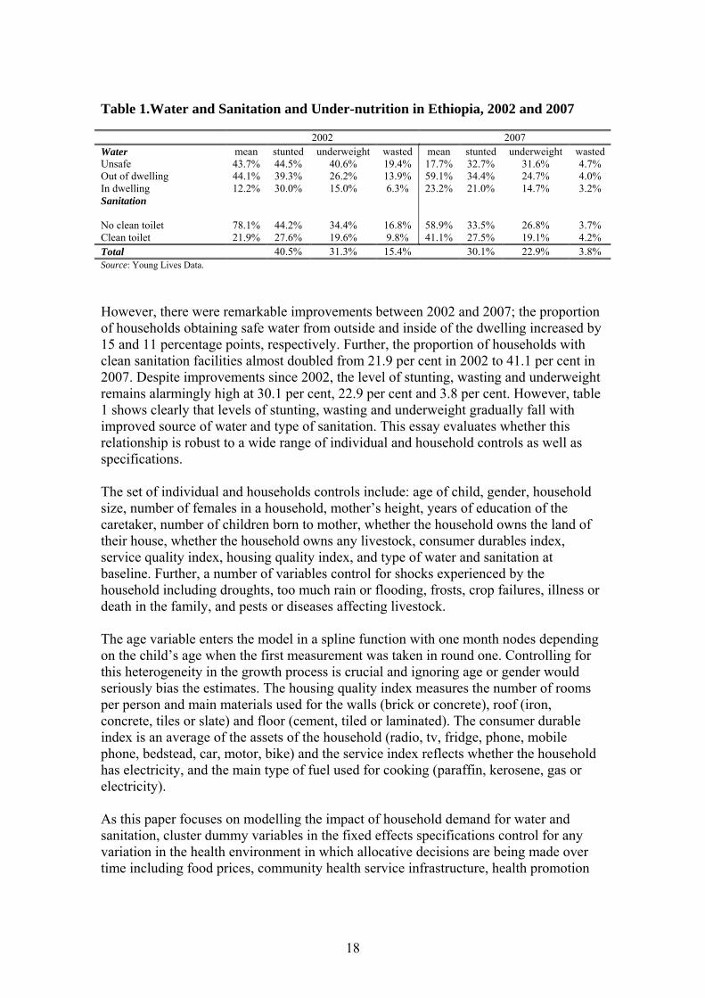
The type of drinking water and sanitation has been classified in line with international standards (WHO and UNICEF 2000). All unprotected surface water sources, such as an unprotected well, a spring, pond or river, are classified as unsafe sources of water. However, even water coming from public wells, though protected, could be contaminated by the time of use. In order to allow for the heterogeneous effects within what qualifies as safe water, an index was constructed that is equal to 0 for unsafe water, 1 for safe water obtained outside of the dwelling (public standpipe, common tap, public well, bore well, piped into neighbours or relatives dwelling/yard), and 2 for safe water coming from inside the dwelling (piped into dwelling/yard/plot). Households who reported ‘bought water’ as their main source of water were classified as obtaining water from outside of the dwelling. Clearly, the use of an index of this type assumes a linear relationship between gradual improvements of water and a child’s z-score. Alternatively, the model has also been estimated using a large number of dummy variables and differences in dummy variables, yielding qualitatively the same results. For type of sanitation, a private pit latrine, septic tank or flush toilet qualify as a clean type of sanitation. Therefore, the index for sanitation is effectively a dummy variable taking on the value of 1 if the household uses a clean type of sanitation, and 0 otherwise. Water and sanitation coverage in Ethiopia is among the lowest worldwide. Official data sources report that 41.2 per cent of households have access to safe water and 21.3 per cent have access to clean sanitation facilities (UNICEF 2007). Table 1 illustrates that the data used in this study find remarkably close numbers for 2002, with 56.3 per cent of households getting water either from outside or inside of the dwelling and 21.9 per cent using a clean type of toilet.

18

Table 1.Water and Sanitation and Under-nutrition in Ethiopia, 2002 and 2007

However, there were remarkable improvements between 2002 and 2007; the proportion of households obtaining safe water from outside and inside of the dwelling increased by 15 and 11 percentage points, respectively. Further, the proportion of households with clean sanitation facilities almost doubled from 21.9 per cent in 2002 to 41.1 per cent in 2007. Despite improvements since 2002, the level of stunting, wasting and underweight remains alarmingly high at 30.1 per cent, 22.9 per cent and 3.8 per cent. However, table 1 shows clearly that levels of stunting, wasting and underweight gradually fall with improved source of water and type of sanitation. This essay evaluates whether this relationship is robust to a wide range of individual and household controls as well as specifications. The set of individual and households controls include: age of child, gender, household size, number of females in a household, mother’s height, years of education of the caretaker, number of children born to mother, whether the household owns the land of their house, whether the household owns any livestock, consumer durables index, service quality index, housing quality index, and type of water and sanitation at baseline. Further, a number of variables control for shocks experienced by the household including droughts, too much rain or flooding, frosts, crop failures, illness or death in the family, and pests or diseases affecting livestock. The age variable enters the model in a spline function with one month nodes depending on the child’s age when the first measurement was taken in round one. Controlling for this heterogeneity in the growth process is crucial and ignoring age or gender would seriously bias the estimates. The housing quality index measures the number of rooms per person and main materials used for the walls (brick or concrete), roof (iron, concrete, tiles or slate) and floor (cement, tiled or laminated). The consumer durable index is an average of the assets of the household (radio, tv, fridge, phone, mobile phone, bedstead, car, motor, bike) and the service index reflects whether the household has electricity, and the main type of fuel used for cooking (paraffin, kerosene, gas or electricity). As this paper focuses on modelling the impact of household demand for water and sanitation, cluster dummy variables in the fixed effects specifications control for any variation in the health environment in which allocative decisions are being made over time including food prices, community health service infrastructure, health promotion

2002 2007 Water mean stunted underweight wasted mean stunted underweight wasted Unsafe 43.7% 44.5% 40.6% 19.4% 17.7% 32.7% 31.6% 4.7% Out of dwelling 44.1% 39.3% 26.2% 13.9% 59.1% 34.4% 24.7% 4.0% In dwelling 12.2% 30.0% 15.0% 6.3% 23.2% 21.0% 14.7% 3.2% Sanitation No clean toilet 78.1% 44.2% 34.4% 16.8% 58.9% 33.5% 26.8% 3.7% Clean toilet 21.9% 27.6% 19.6% 9.8% 41.1% 27.5% 19.1% 4.2% Total 40.5% 31.3% 15.4% 30.1% 22.9% 3.8% Source: Young Lives Data.

19

programs, mosquito infestation, sanitary conditions and political connectedness of the community.

Results

Table 2 presents the pooled OLS results, where water and sanitation appear both as an index in column (1) and (3) as well as dummy variables in column (2) and (4). According to the pooled OLS results, there is a strong positive relationship between use of clean water and sanitation. An increase in the water index by one step leads to an 11% of a standard deviation increase in a child’s z-score. Children who use water from a source in the house have a weight-for-height z-score of 19% of a standard deviation higher compared to children without safe water. The effect is smaller with 0.14 for children who get their water from a source outside of their dwelling and not statistically significant anymore. The presence of a clean type of toilet is highly significant for weight-for-age and is associated with a 20% of a standard deviation higher weight-for-age z-score.

20

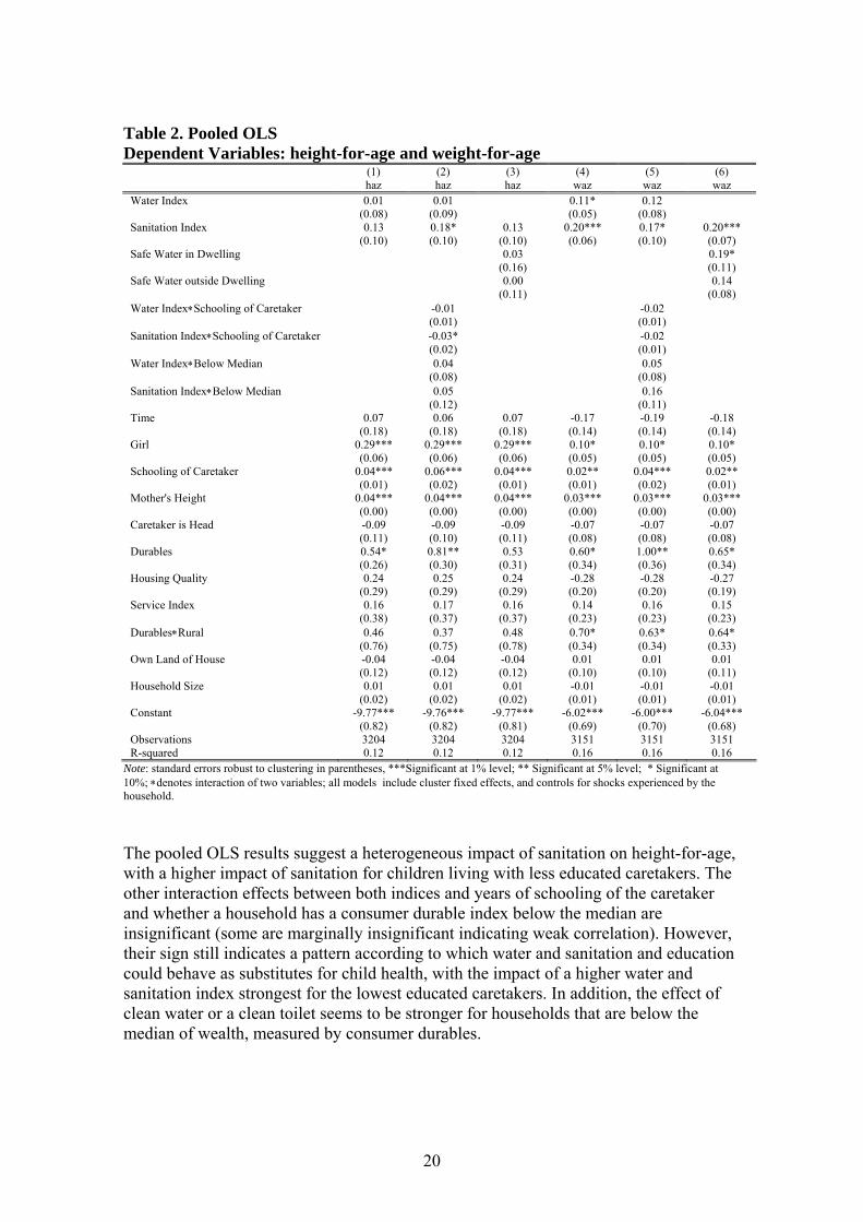
Table 2. Pooled OLS Dependent Variables: height-for-age and weight-for-age

(1) (2) (3) (4) (5) (6) haz haz haz waz waz waz Water Index 0.01 0.01 0.11* 0.12 (0.08) (0.09) (0.05) (0.08) Sanitation Index 0.13 0.18* 0.13 0.20*** 0.17* 0.20*** (0.10) (0.10) (0.10) (0.06) (0.10) (0.07) Safe Water in Dwelling 0.03 0.19* (0.16) (0.11) Safe Water outside Dwelling 0.00 0.14 (0.11) (0.08) Water Index∗Schooling of Caretaker -0.01 -0.02 (0.01) (0.01) Sanitation Index∗Schooling of Caretaker -0.03* -0.02 (0.02) (0.01) Water Index∗Below Median 0.04 0.05 (0.08) (0.08) Sanitation Index∗Below Median 0.05 0.16 (0.12) (0.11) Time 0.07 0.06 0.07 -0.17 -0.19 -0.18 (0.18) (0.18) (0.18) (0.14) (0.14) (0.14) Girl 0.29*** 0.29*** 0.29*** 0.10* 0.10* 0.10* (0.06) (0.06) (0.06) (0.05) (0.05) (0.05) Schooling of Caretaker 0.04*** 0.06*** 0.04*** 0.02** 0.04*** 0.02** (0.01) (0.02) (0.01) (0.01) (0.02) (0.01) Mother's Height 0.04*** 0.04*** 0.04*** 0.03*** 0.03*** 0.03*** (0.00) (0.00) (0.00) (0.00) (0.00) (0.00) Caretaker is Head -0.09 -0.09 -0.09 -0.07 -0.07 -0.07 (0.11) (0.10) (0.11) (0.08) (0.08) (0.08) Durables 0.54* 0.81** 0.53 0.60* 1.00** 0.65* (0.26) (0.30) (0.31) (0.34) (0.36) (0.34) Housing Quality 0.24 0.25 0.24 -0.28 -0.28 -0.27 (0.29) (0.29) (0.29) (0.20) (0.20) (0.19) Service Index 0.16 0.17 0.16 0.14 0.16 0.15 (0.38) (0.37) (0.37) (0.23) (0.23) (0.23) Durables∗Rural 0.46 0.37 0.48 0.70* 0.63* 0.64* (0.76) (0.75) (0.78) (0.34) (0.34) (0.33) Own Land of House -0.04 -0.04 -0.04 0.01 0.01 0.01 (0.12) (0.12) (0.12) (0.10) (0.10) (0.11) Household Size 0.01 0.01 0.01 -0.01 -0.01 -0.01 (0.02) (0.02) (0.02) (0.01) (0.01) (0.01) Constant -9.77*** -9.76*** -9.77*** -6.02*** -6.00*** -6.04*** (0.82) (0.82) (0.81) (0.69) (0.70) (0.68) Observations 3204 3204 3204 3151 3151 3151 R-squared 0.12 0.12 0.12 0.16 0.16 0.16

Note: standard errors robust to clustering in parentheses, ***Significant at 1% level; ** Significant at 5% level; * Significant at 10%; ∗denotes interaction of two variables; all models include cluster fixed effects, and controls for shocks experienced by the household.

The pooled OLS results suggest a heterogeneous impact of sanitation on height-for-age, with a higher impact of sanitation for children living with less educated caretakers. The other interaction effects between both indices and years of schooling of the caretaker and whether a household has a consumer durable index below the median are insignificant (some are marginally insignificant indicating weak correlation). However, their sign still indicates a pattern according to which water and sanitation and education could behave as substitutes for child health, with the impact of a higher water and sanitation index strongest for the lowest educated caretakers. In addition, the effect of clean water or a clean toilet seems to be stronger for households that are below the median of wealth, measured by consumer durables.

21

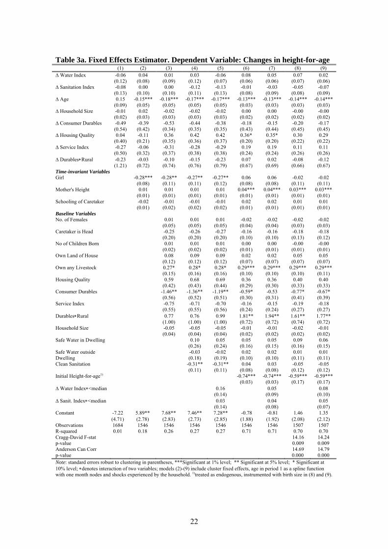
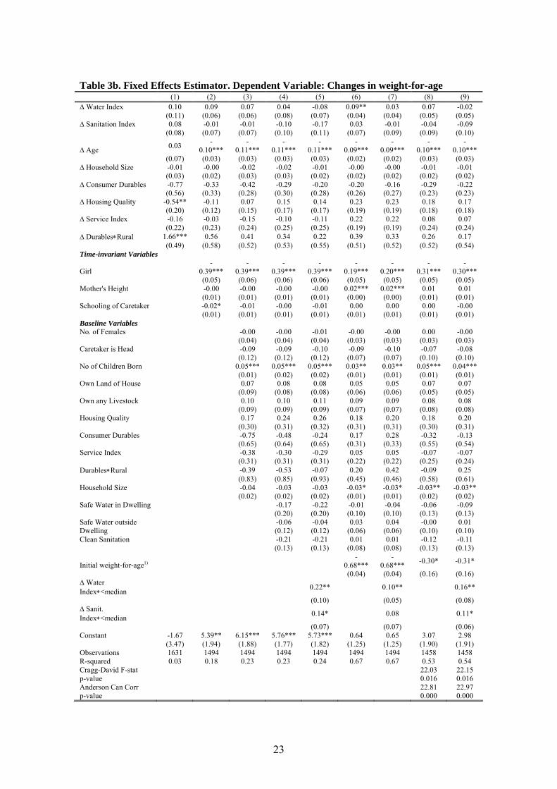
There does not appear to be a systematic difference in height-for-age and weight-for-age z-scores between the two rounds and growth patterns of girls seem to be closer to the reference population. Girls have 29% of a standard deviation higher height-for-age scores and 10% of a standard deviation higher weight-for-age scores compared to boys. The coefficient for the number of years of schooling of the caretaker impacts height-for-age about twice as much as weight-for-age, albeit both effects are small. This might be due to the low level of education in Ethiopia, where the mean is 2.3 years of education among caretakers. The wealth of the household as captured by an index of consumer durables is significant, large in size and positively associated with both height and weight. Differences in weight-for-age attributed to wealth are even more pronounced in rural areas. As discussed above, the pooled OLS estimator is biased in the presence of unobservables that are correlated with the explanatory variables. Tables 3a and 3b test the robustness of the pooled OLS by taking first differences and show the results for height-for-age and weight-for-age. Models (1)-(5) represent the fixed effects estimates to which time-invariant and baseline variables are gradually added as controls to determine the stability of parameters across different model specifications. Columns (6) and (7) show the results of the dynamic conditional demand child growth equation, and the last two columns show results of the dynamic conditional demand child growth equation, where initial height-for-age or weight-for-age z-scores are instrumented with birth size. Models (2)-(6) include dummy variables for the age in months when the first measurement was taken to account for heterogeneity in initial z-scores which drastically change during the period of weaning. To account for differences in the time period between the two measurements, the age difference in months is included as well in all models. Further, models (2)-(9) include cluster fixed effects and dummy variables for shocks experienced by households in period one (results for these control variables are not shown due to space limitations).

22

Table 3a. Fixed Effects Estimator. Dependent Variable: Changes in height-for-age (1) (2) (3) (4) (5) (6) (7) (8) (9) ∆ Water Index -0.06 0.04 0.01 0.03 -0.06 0.08 0.05 0.07 0.02 (0.12) (0.08) (0.09) (0.12) (0.07) (0.06) (0.06) (0.07) (0.06) ∆ Sanitation Index -0.08 0.00 0.00 -0.12 -0.13 -0.01 -0.03 -0.05 -0.07 (0.13) (0.10) (0.10) (0.11) (0.13) (0.08) (0.09) (0.08) (0.09) ∆ Age 0.15 -0.15*** -0.18*** -0.17*** -0.17*** -0.13*** -0.13*** -0.14*** -0.14*** (0.09) (0.05) (0.05) (0.05) (0.05) (0.03) (0.03) (0.03) (0.03) ∆ Household Size -0.01 0.02 -0.02 -0.02 -0.02 0.00 0.00 -0.00 -0.00 (0.02) (0.03) (0.03) (0.03) (0.03) (0.02) (0.02) (0.02) (0.02) ∆ Consumer Durables -0.49 -0.39 -0.53 -0.44 -0.38 -0.18 -0.15 -0.20 -0.17 (0.54) (0.42) (0.34) (0.35) (0.35) (0.43) (0.44) (0.45) (0.45) ∆ Housing Quality 0.04 -0.11 0.36 0.42 0.42 0.36* 0.35* 0.30 0.29 (0.40) (0.21) (0.35) (0.36) (0.37) (0.20) (0.20) (0.22) (0.22) ∆ Service Index -0.27 -0.06 -0.31 -0.28 -0.29 0.19 0.19 0.11 0.11 (0.50) (0.32) (0.37) (0.38) (0.38) (0.24) (0.24) (0.26) (0.26) ∆ Durables∗Rural -0.23 -0.03 -0.10 -0.15 -0.23 0.07 0.02 -0.08 -0.12 (1.21) (0.72) (0.74) (0.76) (0.79) (0.67) (0.69) (0.66) (0.67) Time-invariant Variables Girl -0.28*** -0.28** -0.27** -0.27** 0.06 0.06 -0.02 -0.02 (0.08) (0.11) (0.11) (0.12) (0.08) (0.08) (0.11) (0.11) Mother's Height 0.01 0.01 0.01 0.01 0.04*** 0.04*** 0.03*** 0.03*** (0.01) (0.01) (0.01) (0.01) (0.01) (0.01) (0.01) (0.01) Schooling of Caretaker -0.02 -0.01 -0.01 -0.01 0.02 0.02 0.01 0.01 (0.01) (0.02) (0.02) (0.02) (0.01) (0.01) (0.01) (0.01) Baseline Variables No. of Females 0.01 0.01 0.01 -0.02 -0.02 -0.02 -0.02 (0.05) (0.05) (0.05) (0.04) (0.04) (0.03) (0.03) Caretaker is Head -0.25 -0.26 -0.27 -0.16 -0.16 -0.18 -0.18 (0.20) (0.20) (0.20) (0.10) (0.10) (0.13) (0.12) No of Children Born 0.01 0.01 0.01 0.00 0.00 -0.00 -0.00 (0.02) (0.02) (0.02) (0.01) (0.01) (0.01) (0.01) Own Land of House 0.08 0.09 0.09 0.02 0.02 0.05 0.05 (0.12) (0.12) (0.12) (0.07) (0.07) (0.07) (0.07) Own any Livestock 0.27* 0.28* 0.28* 0.29*** 0.29*** 0.29*** 0.29*** (0.15) (0.16) (0.16) (0.10) (0.10) (0.10) (0.11) Housing Quality 0.59 0.68 0.69 0.36 0.36 0.40 0.40 (0.42) (0.43) (0.44) (0.29) (0.30) (0.33) (0.33) Consumer Durables -1.46** -1.36** -1.19** -0.59* -0.53 -0.77* -0.67* (0.56) (0.52) (0.51) (0.30) (0.31) (0.41) (0.39) Service Index -0.75 -0.71 -0.70 -0.16 -0.15 -0.19 -0.18 (0.55) (0.55) (0.56) (0.24) (0.24) (0.27) (0.27) Durables∗Rural 0.77 0.76 0.99 1.81** 1.94** 1.61** 1.77** (1.00) (1.00) (1.00) (0.72) (0.72) (0.74) (0.72) Household Size -0.05 -0.05 -0.05 -0.01 -0.01 -0.02 -0.01 (0.04) (0.04) (0.04) (0.02) (0.02) (0.02) (0.02) Safe Water in Dwelling 0.10 0.05 0.05 0.05 0.09 0.06 (0.26) (0.24) (0.16) (0.15) (0.16) (0.15) Safe Water outside -0.03 -0.02 0.02 0.02 0.01 0.01 Dwelling (0.18) (0.19) (0.10) (0.10) (0.11) (0.11) Clean Sanitation -0.31** -0.31** 0.04 0.03 -0.05 -0.05 (0.11) (0.11) (0.08) (0.08) (0.12) (0.12) Initial Height-for-age1) -0.74*** -0.74*** -0.59*** -0.59*** (0.03) (0.03) (0.17) (0.17) ∆ Water Index∗<median 0.16 0.05 0.08 (0.14) (0.09) (0.10) ∆ Sanit. Index∗<median 0.03 0.04 0.05 (0.14) (0.08) (0.07) Constant -7.22 5.89** 7.68** 7.46** 7.28** -0.78 -0.81 1.46 1.35   (4.71) (2.78) (2.83) (2.73) (2.85) (1.88) (1.92) (2.08) (2.12) Observations 1684 1546 1546 1546 1546 1546 1546 1507 1507 R-squared 0.01 0.18 0.26 0.27 0.27 0.71 0.71 0.70 0.70 Cragg-David F-stat 14.16 14.24 p-value 0.009 0.009 Anderson Can Corr 14.69 14.79 p-value 0.000 0.000 Note: standard errors robust to clustering in parentheses, ***Significant at 1% level; ** Significant at 5% level; * Significant at 10% level; ∗denotes interaction of two variables; models (2)-(9) include cluster fixed effects, age in period 1 as a spline function with one month nodes and shocks experienced by the household. 1)treated as endogenous, instrumented with birth size in (8) and (9).

23

Table 3b. Fixed Effects Estimator. Dependent Variable: Changes in weight-for-age (1) (2) (3) (4) (5) (6) (7) (8) (9) ∆ Water Index 0.10 0.09 0.07 0.04 -0.08 0.09** 0.03 0.07 -0.02 (0.11) (0.06) (0.06) (0.08) (0.07) (0.04) (0.04) (0.05) (0.05) ∆ Sanitation Index 0.08 -0.01 -0.01 -0.10 -0.17 0.03 -0.01 -0.04 -0.09 (0.08) (0.07) (0.07) (0.10) (0.11) (0.07) (0.09) (0.09) (0.10)

∆ Age 0.03 -0.10***

-0.11***

-0.11***

-0.11***

-0.09***

-0.09***

-0.10***

-0.10***

(0.07) (0.03) (0.03) (0.03) (0.03) (0.02) (0.02) (0.03) (0.03) ∆ Household Size -0.01 -0.00 -0.02 -0.02 -0.01 -0.00 -0.00 -0.01 -0.01 (0.03) (0.02) (0.03) (0.03) (0.02) (0.02) (0.02) (0.02) (0.02) ∆ Consumer Durables -0.77 -0.33 -0.42 -0.29 -0.20 -0.20 -0.16 -0.29 -0.22 (0.56) (0.33) (0.28) (0.30) (0.28) (0.26) (0.27) (0.23) (0.23) ∆ Housing Quality -0.54** -0.11 0.07 0.15 0.14 0.23 0.23 0.18 0.17 (0.20) (0.12) (0.15) (0.17) (0.17) (0.19) (0.19) (0.18) (0.18) ∆ Service Index -0.16 -0.03 -0.15 -0.10 -0.11 0.22 0.22 0.08 0.07 (0.22) (0.23) (0.24) (0.25) (0.25) (0.19) (0.19) (0.24) (0.24) ∆ Durables∗Rural 1.66*** 0.56 0.41 0.34 0.22 0.39 0.33 0.26 0.17 (0.49) (0.58) (0.52) (0.53) (0.55) (0.51) (0.52) (0.52) (0.54) Time-invariant Variables

Girl -0.39***

-0.39***

-0.39***

-0.39***

-0.19***

-0.20***

-0.31***

-0.30***

(0.05) (0.06) (0.06) (0.06) (0.05) (0.05) (0.05) (0.05) Mother's Height -0.00 -0.00 -0.00 -0.00 0.02*** 0.02*** 0.01 0.01 (0.01) (0.01) (0.01) (0.01) (0.00) (0.00) (0.01) (0.01) Schooling of Caretaker -0.02* -0.01 -0.00 -0.01 0.00 0.00 0.00 -0.00 (0.01) (0.01) (0.01) (0.01) (0.01) (0.01) (0.01) (0.01) Baseline Variables No. of Females -0.00 -0.00 -0.01 -0.00 -0.00 0.00 -0.00 (0.04) (0.04) (0.04) (0.03) (0.03) (0.03) (0.03) Caretaker is Head -0.09 -0.09 -0.10 -0.09 -0.10 -0.07 -0.08 (0.12) (0.12) (0.12) (0.07) (0.07) (0.10) (0.10) No of Children Born 0.05*** 0.05*** 0.05*** 0.03** 0.03** 0.05*** 0.04*** (0.01) (0.02) (0.02) (0.01) (0.01) (0.01) (0.01) Own Land of House 0.07 0.08 0.08 0.05 0.05 0.07 0.07 (0.09) (0.08) (0.08) (0.06) (0.06) (0.05) (0.05) Own any Livestock 0.10 0.10 0.11 0.09 0.09 0.08 0.08 (0.09) (0.09) (0.09) (0.07) (0.07) (0.08) (0.08) Housing Quality 0.17 0.24 0.26 0.18 0.20 0.18 0.20 (0.30) (0.31) (0.32) (0.31) (0.31) (0.30) (0.31) Consumer Durables -0.75 -0.48 -0.24 0.17 0.28 -0.32 -0.13 (0.65) (0.64) (0.65) (0.31) (0.33) (0.55) (0.54) Service Index -0.38 -0.30 -0.29 0.05 0.05 -0.07 -0.07 (0.31) (0.31) (0.31) (0.22) (0.22) (0.25) (0.24) Durables∗Rural -0.39 -0.53 -0.07 0.20 0.42 -0.09 0.25 (0.83) (0.85) (0.93) (0.45) (0.46) (0.58) (0.61) Household Size -0.04 -0.03 -0.03 -0.03* -0.03* -0.03** -0.03** (0.02) (0.02) (0.02) (0.01) (0.01) (0.02) (0.02) Safe Water in Dwelling -0.17 -0.22 -0.01 -0.04 -0.06 -0.09 (0.20) (0.20) (0.10) (0.10) (0.13) (0.13) Safe Water outside -0.06 -0.04 0.03 0.04 -0.00 0.01 Dwelling (0.12) (0.12) (0.06) (0.06) (0.10) (0.10) Clean Sanitation -0.21 -0.21 0.01 0.01 -0.12 -0.11 (0.13) (0.13) (0.08) (0.08) (0.13) (0.13)

Initial weight-for-age1) -0.68***

-0.68*** -0.30* -0.31*

(0.04) (0.04) (0.16) (0.16) ∆ Water Index∗<median 0.22** 0.10** 0.16**

(0.10) (0.05) (0.08) ∆ Sanit. Index∗<median 0.14* 0.08 0.11*

(0.07) (0.07) (0.06) Constant -1.67 5.39** 6.15*** 5.76*** 5.73*** 0.64 0.65 3.07 2.98 (3.47) (1.94) (1.88) (1.77) (1.82) (1.25) (1.25) (1.90) (1.91) Observations 1631 1494 1494 1494 1494 1494 1494 1458 1458 R-squared 0.03 0.18 0.23 0.23 0.24 0.67 0.67 0.53 0.54 Cragg-David F-stat 22.03 22.15 p-value 0.016 0.016 Anderson Can Corr 22.81 22.97 p-value 0.000 0.000

24

Note: standard errors robust to clustering in parentheses, ***Significant at 1% level; ** Significant at 5% level; * Significant at 10% level; ∗denotes interaction of two variables; models (2)-(9) include cluster fixed effects, age in period 1 as a spline function with one month nodes and shocks experienced by the household. 1)treated as endogenous, instrumented with birth size in (8) and (9). The results show that removing the time-invariant unobservables and controlling for the impact of time-invariant as well as time-variant variables across time reduces the impact of water and sanitation on height-for-age to zero across almost all models, if not interacted with wealth. Only model (6) in the weight-for-age regressions suggests that children from households that experienced a one unit increase in the drinking water index, enjoyed 0.09 of a standard deviation higher growth of weight-for-age z-scores between the two periods. The coefficient is surprisingly similar to the coefficient obtained in column (2), however, insignificant in the other specifications. This suggests that the coefficients obtained from the pooled OLS estimator are seriously biased upwards. Further, the results indicate that children from families who had a safe source of drinking water in the base period did not have higher catch-up effects compared to those who did not have a safe source of drinking water. On the contrary, column (4) and (5) suggest that the presence of a toilet leads to a 0.3 smaller change in z-scores. This exemplifies the need to condition on initial height-for-age and employ a dynamic model, since the negative coefficient could be biased due to individual heterogeneity in period one; in other words, children who had a clean type of toilet in period one were healthier and thus had less need to catch-up. This proves to be the case, as the inclusion of the initial height-for-age z-score results in making the variable insignificant. The same pattern arises with weight-for-age, where dummy variable for safe type of toilet is marginally significant in column (4) and (5), indicating that the presence of a toilet resulted in lower changes in weight-for-age but becomes insignificant as the control for initial weight-for-age is included. Lagged height-for-age and weight-for-age z-scores enter the models significantly and negatively, suggesting that partial catch-up takes place. A value of -1 would imply full catch-up, while a coefficient not significantly different from zero would imply that the dynamic specification is superfluous and changes in the z-scores are independent of initial conditions. Instrumenting for the lagged z-scores with birth size slightly decreases the size of the coefficient on the initial height-for-age z-score, and more than halves the coefficient on the initial weight-for-age z-score. Nevertheless, after instrumenting they both remain significant determinants of changes in a child’s z-scores over the two periods. As discussed in the model section of this paper, this indicates that the coefficient on the lagged dependent variable was biased downwards when not instrumented, which is what was expected due to the negative correlation between the lagged dependent variable and the residuals. The Anderson canonical correlations test and the Cragg-Donald F-statistic suggest for the height-for-age as well as for the weight-for-age regressions that the null hypothesis of underidentification can be rejected. The interaction effects investigate whether the impact of an improvement in water and sanitation is heterogeneous across households depending on the wealth level of the household and education level of the caretaker. While the interaction effects are insignificant for changes in height-for-age, improvements in water and sanitation facilities appear to have a substantial effect on weight-for-age, in particular for children

25

from families below the median wealth level. An increase in the water index for households which lie below the median of the consumer durables index results in a 10 - 22 per cent of a standard deviation higher change in weight-for-age z-scores between the two periods. An increase in the sanitation index by one for households below the median leads to a 8 - 14 per cent of a standard deviation higher growth of weight-for-age. The interaction effects in the model for weight-for-age are robust to the inclusion of the lagged dependent variable, and the instrumented lagged dependent variable. This implies that investments in improved water and sanitation can have particularly high returns to child health for the poorest households if it is reflected in higher usage. In the same spirit, changes in the water and sanitation indices were also interacted with the number of years of schooling of the caretaker. The coefficients were insignificant, implying that there are no heterogeneous impacts depending on the level of education of the caretaker, which is in contradiction with Barrera (1990). The difference between the pooled OLS (table 2) and the first differences (tables 3a and 3b) is nevertheless striking, and the results obtained in the differenced equation which eliminates individual and household fixed effects, present a rather different picture. They point towards a much stronger effect for the poorest households from improvements in usage patterns of water and sanitation, once time-invariant heterogeneity has been taken into account. It is important to note that the inclusion of the lagged dependent variable changes the interpretation of the coefficients and the above discussion refers to the short run impact of these coefficients. To calculate the long run effects, the short run coefficients have to be divided by the coefficient on the lagged dependent variable (see model specification (13) in section three). Using the results of the instrumented equation from column (9) of table 3b, a one unit improvement in the water index for the poorest households would yield a 52 per cent of a standard deviation higher weight-for-age z-score in the long run, more than 3 times the short run effect. The long run effect of a one unit increase in the sanitation index leads to a 35 per cent of a standard deviation higher weight-for-age z-score. If the models are correctly specified, this implies that the estimates in column (5) present a lower bound of the impact of water and sanitation. Looking at the other explanatory variables, the results suggest that girls have smaller increases in z-scores compared to boys, and this is robust to accounting for initial conditions through the lagged dependent variable for weight-for-height, but the effect disappears for height-for-age once individual heterogeneity is controlled for. Mother’s height capturing genetic endowments is a significant determinant of height-for-age only in the dynamic specifications, where the coefficient is slightly smaller when lagged height-for-age is instrumented. A one standard deviation increase in mother’s height leads to an increase in a child’s height-for-age z-score of 18-24 per cent of a standard deviation. For weight-for-age, mother’s height is significant in the dynamic model, suggesting a 12 per cent of a standard deviation increase in a child’s weight-for-age z-score for a one standard deviation increase in mother’s height, but is not significant anymore when instrumenting for the lagged dependent variable. The ownership of livestock leads to a 27 per cent of a standard deviation higher growth height-for-age z-scores, which is robust across all specifications, but is insignificant for weight-for-age. Due to the fact that the ownership of consumer durables is very low, in particular in rural areas, it might be the most appropriate measure of wealth. Additionally, livestock might be an important consumption smoothing device in an environment with frequent

26

shocks and thus facilitate catch-up after a shock. Children from families with more consumer durables tend to have lower changes in height-for-age over the period. This could be the case if children from wealthier families are better off already in the first period and therefore have less scope for catching up between the two periods. When accounting for initial conditions through the inclusion of the lagged dependent variable the coefficient roughly halves in size, but nevertheless remains significant, which is counter intuitive. When consumer durables are interacted with a dummy variable that equals one if the household resides in a rural area, the parameter becomes significant and large in size in the dynamic model. Consequently, while children from richer families in urban environments catch-up less in height-for-age, children from richer families in rural areas tend to have large improvements in their z-scores. Children whose mothers had a higher number of children at baseline tend to have higher growth of weight-for-age z-scores. This could be due to intra-household allocation where families with healthier children tend to have more children. While the effect of changes in water and sanitation favouring the children of the poor is remarkably robust across the different model specifications, three further considerations should be made when judging the validity of these results. First, despite the comprehensive set of individual and household controls, as well as controlling for unobserved time-invariant individual and households fixed effects, concerns remain relating to how far the model has succeeded to control for endogeneity of the water and sanitation variable. Given the difficulty of finding instruments that can credibly be excluded from the model, a large range of controls is the best bet to limit the bias of the estimators. Second, a further reason for concern is that, although attrition is very low in the present panel, it has been found to be non-random, and the probability of attrition is correlated with low anthropometric indicators (Dercon and Outes-Leon, 2007). One way to determine whether unobservables affecting attrition are correlated with unobservables affecting child health, would be through a Heckman Selection model. However, this hinges upon finding a valid exclusion restriction, and it is difficult to find a variable that is correlated with the probability of survival of a child but does not affect a child’s nutritional status later other than through survival. A final consideration relates to the limitations of the data, which do not have certain variables that would be desirable to include. There are no data on health inputs, such as nutritional data in both time periods, which would allow testing for substitution and changes in intra-household allocation. Further, there is no information regarding the time spent fetching water, which impacts the household’s choice of which source of water to use, gains in terms of time saved from a closer water source, and frequency of water fetching which in turn affects storing practices. Other variables that impact the degree to which clean water has a beneficial impact relate to the quantity of water provided by water source, as well as whether livestock is kept away from water, whether water coming from domestic pipes is rationed and the quality of indoor plumbing.

Conclusion

This essay presents a departure from the literature evaluating access to water and sanitation on child health by investigating the impact of households’ usage patterns of water and sanitation on the health of children in Ethiopia, after controlling for supply side factors, such as the health environment, community health infrastructure and health

27

promotion programs through cluster fixed effects. A comprehensive set of controls was employed to account for individual heterogeneity driven by time-invariant unobservables, time-invariant and time-variant observables. The obtained results from the pooled cross-section estimated by OLS suggest that there is a strong relationship between water and sanitation choices of a household and a child’s weight-for-age z-scores. This correlation disappears when unobserved time-invariant fixed effects are removed through a fixed effects specification. However, the fixed effects model reveals that children from the poorest families who shifted to improved water and sanitation usage patterns exhibited a significantly larger growth in weight-for-age z-scores between the two periods. The effect remains robust to a number of different specifications, including a dynamic model and instrumented version of a dynamic model, allowing for catch-up and other sources of dynamic heterogeneity correlated with initial levels of nutrition. Consequently, the effectiveness of investments in water and sanitation infrastructure can be leveraged by influencing the choices made by households on the type of water and sanitation, bringing the greatest benefits to children of most deprived families. Of course, the non-experimental nature of the data presents a limitation to the findings of this study. A strong effort has been made to purge the estimates from potential endogeneity bias through the fixed effects transformation and a large number of controls. Further research efforts could be directed towards exploring the constraints households face when making choices regarding water and sanitation; these include constraints related to the use of safe source of water include the distance to the nearest source of water, transport options and the quantity of water available (and potential rationing), which determine the price of clean water to the household; the importance of cultural factors and tradition in uptake of latrines and resulting implications for programme design. Collecting data on these variables would shed further light on context-specific underlying constraints households face and help design programs that take these into account. This would also involve research on the most effective communication strategies to increase households’ awareness and engagement to choose a safe source of water and clean sanitation. Many children in Ethiopia and around the world grow up undernourished and in poor water and sanitary conditions. The opportunity of extracting the highest return to child health from investments in water and sanitation infrastructure, when reflected in usage of better sources of water and types of sanitation, should not be missed.

28

Bibliography

Alderman, Harold, Jesko Hentschel and Ricardo Sabates (2003) ‘With the help of one’s neighbours: externalities in the production of nutrition in Peru’, Social Science & Medicine 56: 2019-2031 Arellano, Manuel and Stephen Roy Bond, (1991) ‘Some Tests of Specification for Panel Data: Monte Carlo Evidence and an Application to Employment Equations’, The Review of Economic Studies 58.2:277-297 Ayele, Manyahlshal (2005) Water is life, Sanitation is Dignity: Sanitation preference and household latrine designs, Briefing Note 1, Ethiopia: Water Aid Ethiopia Barrera, Albino (1990) ‘The role of maternal schooling and its interaction with public health programs in child health production’, Journal of Development Economics 32.1:69-91 Baum, Christopher, Stephen Stillman and Mark Schaffer (2007) Enhanced routines for instrumental variables/GMM estimation and testing, Boston College Working Papers in Economics 667, Chestnut Hill:Boston College Department of Economics Behrman, Jere R. and Anil B. Deolalikar (1988) ‘Health and Nutrition’, in H.Chenery and T.N. Srinivasan (eds.) Handbook of Development Economics, Volume 1 Behrman, Jere R. (1996) ‘Impact of Health and Nutrition on Education’, World Bank Research Observer 11.1: 23-37 Burger, Susan E., and Stephen A. Esrey (1995) ‘Water and sanitation: health and nutrition benefits to children’, in Per Pinstrup-Andersen, David Pelletier and Harold Alderman (eds.) Child Growth and Nutrition in Developing Countries: Priorities for Action, Ithaca: Cornell University Press Caulfield, Laura E., Mercedes de Onis, Monika Bloessner and Robert E Black (2004) ‘Undernutrition as an underlying cause of child deaths associated with diarrhea, pneumonia, malaria and measles’, American Journal of Clinical Nutrition 80:193-8 Checkley, William, Robert H Gilman, Robert E Black, Leonardo D Epstein, Lilia Cabrera, Charles R Sterling and Lawrence H Moulton (2004) ‘Effect of water and sanitation on childhood health in a poor Peruvian peri-urban community’, Lancet 363:112-18 De Onis, Mercedes, Adelheid.W. Onyango, Elaine Borghi, Amani Siyam, Chizuru Nishida and Jonathan Siekmann (2007) ‘Development of a WHO growth reference for school-aged children and adolescents’, Bulletin of the World Health Organization 85: 660-7

29

Deaton, Angus S. (1997) The analysis of household surveys: A microeconometric approach to development policy, Baltimore MD: Johns Hopkins University Press Dercon, Stefan and Ingo Outes-Leon (2007) Survey Attrition and Attrition Bias in the Young Lives Study, mimeo Esrey, Stephen A. (1996) ‘Water, waste and well-being: a multicounty study’, American Journal of Epidemiology 143:608-623 Esrey, Stephen A., and Jean-Pierre Habicht (1988) ‘Maternal literacy modifies the effect of toilets and piped water on infant survival in Malaysia’, American Journal of Epidemiology 127.5: 1079-1087 Esrey, Stephen A., Jean-Pierre Habicht and George Casella (1992) ‘The complementary effect of latrines and increased water usage on the growth of infants in rural Lesotho’, American Journal of Epidemiology 135.6: 659-666 Federov, Leonid, and David E. Sahn (2005) ‘Socioeconomic Determinants of Children’s Health in Russia: A Longitudinal Study’, Economic Development and Cultural Change 53.2:479-500 Foster, Andrew (1995) ‘Prices, credit markets and child growth in low-income rural areas’, Economic Journal 105: 551-70 Gragnolati, Michele (1999) Children’s Growth and Poverty in Rural Guatemala, Policy Research Working Paper 2193, Washington D.C.: World Bank Haddad, Lawrence, Harold Alderman, Simon Appleton, Lina Song, Yisehac Yohannes (2003) ‘Reducing Child Malnutrition: How far does Income Growth take us?’, The World Bank Economic Review 17.1: 107-131 Hoddinott, John (1997) Water, Health and Income: a Review, Discussion paper no. 25, Washington D.C.: International Food Policy Research Institute Hoddinott, John, and Bill Kinsey (2001) ‘Child Growth in the Time of Drought’, Oxford Bulletin of economics and statistics, 63.4: 409-436 Jalan, Jyotsna, and Martin Ravallion (2003) ‘Does Piped Water Reduce Diarrhea for Children in Rural India?’, Journal of Econometrics 112: 153-173 Lavy, Victor Chaim, John Strauss, Duncan Thomas and Philippe de Vreyer (1996) ‘Quality of Health Care, Survival and Health Outcomes in Ghana’, Journal of Health Economics 15:333-357 Lee, Lung-fei, Mark R. Rosenzweig and Mark M. Pitt (1997) ‘The Effects of Improved Nutrition, Sanitation and Water Quality on Child Health in High-Mortality Populations’, Journal of Econometrics 77: 209-235

30

Matorell, Reynaldo, Laura Kettel-Khan and Dirk G. Schroeder (1994) ’Reversibility of Stunting: Epidemiological Findings in Children from Developing Countries’, European Journal of Clinical Nutrition 48 (Supplement I):S45-S57 Merchant, Anwar T., Clara Jones, Anamaria Kiure, Roland Kupka, Garrett Fitzmaurice, M.Guillermo Herrera and Wafaie W Fawzil (2003) ’Water and sanitation associated with improved child growth’, European Journal of Clinical Nutrition 57:1562–1568 Payne, Philip (1993) Assessing Undernutrition: The need for a reconceptualization, in Siddiqur Rahman Osmani (ed.), Nutrition and Poverty, Oxford: Clarendon Press Pelletier, David L., Edward A.Frongillo, Dirk G. Schroeder and Jean-Pierre Habicht (1995) ‘The effects of malnutrition on child mortality in developing countries’, Bulletin of the World Health Organisation 73.4: 443-8. Pitt, Mark M. (1993) ‘Analyzing Human Resources: Health’, in Lionel Demery, Marco Ferroni and Christiaan Grootaert with Jorge Wong-Valle (eds.) Understanding the Social Effects of Policy Reform, Washington D.C.: World Bank

31

Pollitt, Ernesto, Kathleen S. Gorman, Patrice L Engle, Reynaldo Martorell, Juan Rivera, Theodore D. Wachs, and Nevin S. Scrimshaw (1993) ‘Early Supplementary Feeding and Cognition: Effects over Two Decades’, Monographs of the Society for Research in Child Development 58.7: 1-118 Rosenzweig, Mark .R. and Kenneth I. Wolpin (1986) ‘Evaluating the effects of optimally distributed public programs: child health and family planning interventions’, American Economic Review 76:470–482 Strauss, John and Duncan Thomas (1998) ‘Health, Nutrition, and Economic Development’, Journal of Economic Literature 36.2: 766-817 Strauss, John and Duncan Thomas (2008) ‘Health over the life course’, in T.Paul Schultz and John Strauss (eds.), Handbook of Development Economics Volume 4, Amsterdam: North Holland Press Strauss, John (1990) ‘Households, communities, and preschool children’s nutrition outcomes: Evidence from rural Côte d’Ivoire’, Economic Development and Cultural Change 38.2:231-262 Thomas, Duncan and John Strauss (1992) ‘Prices, infrastructure, household characteristics and child height’, Journal of Development Economics 39.2:301-331 United Nations Children Fund (2007) ‘Background Brief, UNICEF Ethiopia’s Water and Sanitation (WES) Programme’, http://www.unicef.org/ethiopia/ET_WES_background.pdf (accessed June 08) Woldemicael Gebremariam (2000) ‘The effects of water supply and sanitation on childhood mortality in urban Eritrea’, Journal of Biosocial Science 32.2:207-27 Wooldridge, Jeffrey M. (2002) Econometric Analysis of Cross Section and Panel Data, Cambridge MA: MIT Press Wooldridge, Jeffrey M. (2006) ‘Cluster sample methods in applied econometrics: an extended analysis’, http://www.msu.edu/~ec/faculty/wooldridge/current%20research/clus1aea.pdf (accessed June 08) World Bank. (2005a) Ethiopia: Well-being and Poverty in Ethiopia: The Role of Agriculture and Agency, Washington, D.C.: World Bank World Bank (2005b) Ethiopia: A Country Status Report on Health and Poverty, Washington, D.C.: World Bank World Bank (2007) Ethiopia: Capturing the Demographic Bonus in Ethiopia: Gender, Development, and Demographic Actions, Washington, D.C.: World Bank

32

World Bank. (2008a). ‘Ethiopia Country Brief’, http://go.worldbank.org/WA1RL12OL0 (accessed June 08) World Bank. (2008b). World Development Report: Agriculture for Development, Washington, D.C.: World Bank World Health Organisation (1995) Physical Status: The Use and Interpretation of Anthropometry, WHO Technical Report No. 854, Geneva: World Health Organisation World Health Organisation (2007) WHO Child Growth Standards: Methods and development, Geneva: World Health Organisation World Health Organisation and United Nations Children Fund (2000) Global Water Supply and Sanitation Assessment 2000 Report, The WHO and UNICEF Joint Monitoring Programme for Water Supply and Sanitation (JMP). Yamano, Takashi, Harold Alderman and Luc Christiaensen (2005) ‘Child Growth, Shocks and Food Aid in Rural Ethiopia’, American Journal of Agricultural Economics, 87.2:273-288

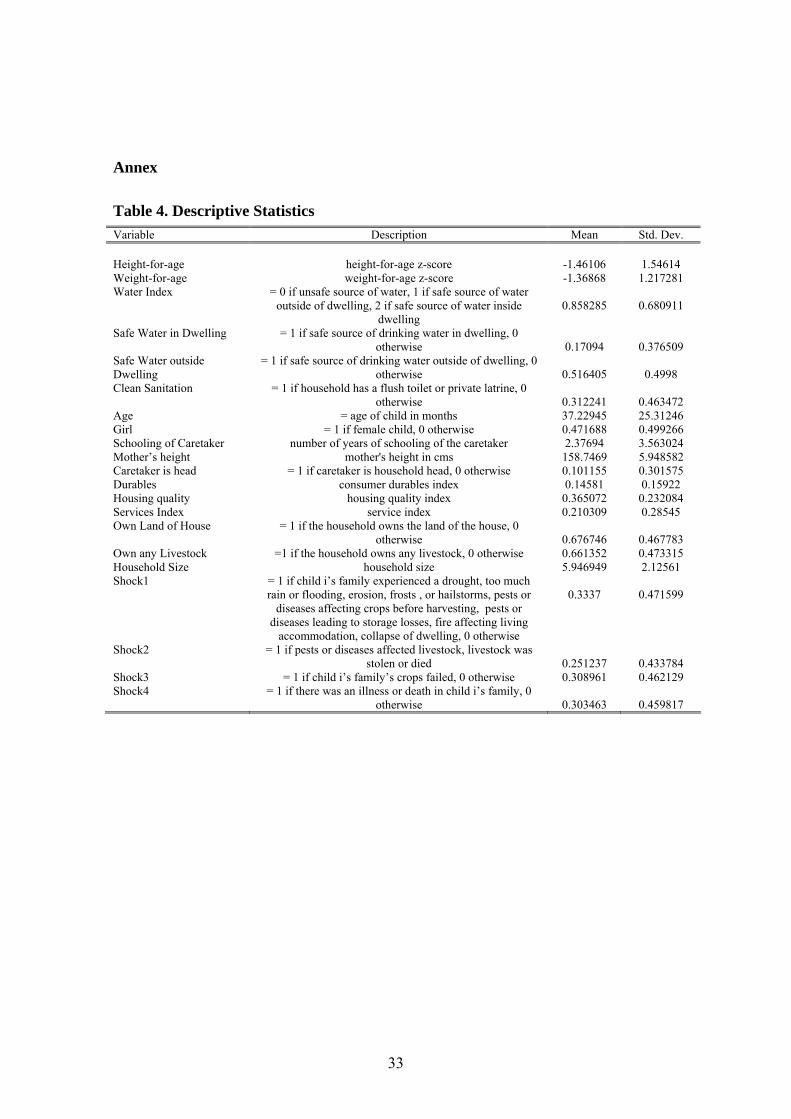
33

Annex

Table 4. Descriptive Statistics

Variable Description Mean Std. Dev. Height-for-age height-for-age z-score -1.46106 1.54614 Weight-for-age weight-for-age z-score -1.36868 1.217281 Water Index

= 0 if unsafe source of water, 1 if safe source of water outside of dwelling, 2 if safe source of water inside

dwelling 0.858285

0.680911

Safe Water in Dwelling = 1 if safe source of drinking water in dwelling, 0

otherwise 0.17094 0.376509 Safe Water outside Dwelling

= 1 if safe source of drinking water outside of dwelling, 0 otherwise 0.516405 0.4998

Clean Sanitation = 1 if household has a flush toilet or private latrine, 0 otherwise 0.312241 0.463472

Age = age of child in months 37.22945 25.31246 Girl = 1 if female child, 0 otherwise 0.471688 0.499266 Schooling of Caretaker number of years of schooling of the caretaker 2.37694 3.563024 Mother’s height mother's height in cms 158.7469 5.948582 Caretaker is head = 1 if caretaker is household head, 0 otherwise 0.101155 0.301575 Durables consumer durables index 0.14581 0.15922 Housing quality housing quality index 0.365072 0.232084 Services Index service index 0.210309 0.28545 Own Land of House = 1 if the household owns the land of the house, 0

otherwise 0.676746 0.467783 Own any Livestock =1 if the household owns any livestock, 0 otherwise 0.661352 0.473315 Household Size household size 5.946949 2.12561 Shock1

= 1 if child i’s family experienced a drought, too much rain or flooding, erosion, frosts , or hailstorms, pests or

diseases affecting crops before harvesting, pests or diseases leading to storage losses, fire affecting living

accommodation, collapse of dwelling, 0 otherwise

0.3337

0.471599

Shock2 = 1 if pests or diseases affected livestock, livestock was stolen or died 0.251237 0.433784

Shock3 = 1 if child i’s family’s crops failed, 0 otherwise 0.308961 0.462129 Shock4 = 1 if there was an illness or death in child i’s family, 0

otherwise 0.303463 0.459817