Do firms benefit from their relationships with credit ... · Do firms benefit from their relationships with credit unions ... by disentangling bank credit supply ... the banking relationship

Do firms benefit from their relationships with

credit unions during dire times?

Leila Aghabarari†

Andre Guettler‡

Mahvish Naeem§

Bernardus Van Doornik**

Credit unions (CUs) are unique financial intermediaries because of their membership-based governance structure. We exploit the financial crisis of 2008/09 as a negative shock to Brazilian banks and analyze the variation in the lending behavior of CUs versus non-CUs and the subsequent effects on the commercial clients’ labor force. We find evidence that during the financial crisis, CUs tightened access to credit to their members to a lesser extent (insurance effect) than did other bank types. Moreover, compared to non-CUs during the crisis, CUs provided credit with longer maturities and required less collateral, albeit at higher interest rates. Notwithstanding, CUs did not display higher risk on their credit portfolios in comparison to other banks in the crisis period. However, CUs faced relatively higher future default frequencies. Notably, the labor market impact of the insurance effect of CUs is positive for very small firms in the form of an increase in employment and wages in the crisis period.

Keywords: Credit unions, Financial intermediaries, Financial crisis, Relationship lending, Labor market outcomes

JEL: G01, G21, J21, J31

The Working Papers should not be reported as representing the views of the Banco Central do Brasil. The views expressed in the papers are those of the author(s) and do not necessarily reflect those of the Banco Central do Brasil, International Bank for Reconstruction and Development/World Bank and its affiliated organizations, or those of the Executive Directors of the World Bank or the governments they represent.

† World Bank Group, 1818 H St NW, Washington DC, 20433. E-mail: [email protected]. ‡ Ulm University, Institute of Strategic Management and Finance, Helmholtzstraße 22, 89081 Ulm, Germany and Institute for Economic Research Halle (IWH), E-mail: [email protected] (corresponding author). § Ulm University, Institute of Strategic Management and Finance, Helmholtzstraße 22, 89081 Ulm, Germany, E-mail: [email protected]. ** Central Bank of Brazil, Research Department, Setor Bancário Sul Quadra 3 Bloco B - Ed. Sede, CEP: 70074-900 Brasília, Brazil, E-mail: [email protected]. Declarations of interest: none

1

I. Introduction

Bank financing is a crucial source of funding for businesses. Hence, disruptions in bank

lending activity can be the cause of adverse shocks to the real economy. When a financial crisis

unfolds, access to finance tightens because banks cut back credit supply. This adversely affects

growth. Financial crisis has impact on the real economy largely through deterioration of the

outcomes of bank-dependent firms (e.g., Hoshi and Kashyap, 1990; Morck et al., 2001; Bayoumi

and Lipworth, 1999; Chava and Purnanandam, 2011; Paravisini, 2008).

On the occasion that all financial institutions react to a shock with the same intensity, the

economic consequences of the credit crunch can be irreparable. However, there is empirical

evidence that during the crisis, some types of banks curtail their lending less than others. For

example, government-owned banks increase the supply of credit compared to private banks, which

decrease lending during the crisis (Coleman and Feler, 2015). Additionally, financial constraints

are more likely to be prevalent among local banks compared to foreign banks (Paravisini, 2008).

Hence, the literature provides evidence that a diversified banking industry could cope better with

a financial crisis.

Most recent empirical work has focused on bank lending behavior during the financial

crisis of 2008/09. However, alternative financial institutions have received little academic

attention. We attempt to fill this gap in this literature by exploring credit unions (CUs), as they are

different in terms of governance and ownership structure. We study the transmission of liquidity

shocks in the Brazilian banking market using the financial crisis of 2008/09 as a natural laboratory.

We examine whether CUs can provide countercyclical support during the financial crisis and

whether this comfort transmits to the real economy.

2

Our focus is on CUs because they are prototypical local lenders to retail clients and small

and medium enterprises (SMEs). The peculiarity of CUs concerns their cooperative nature. These

intermediaries collect deposits from their members and provide their members with asset

transformation into loans. Each member has one vote without regard to the volume of equity they

have invested in the CU. Thus, any reduction of credit supply during dire times may be less

pronounced given that members not only are driven by profit maximization of their equity

investment but are also interested in attractive loan terms and alleviating credit constraints

(Angelini, Di Salvo, and Ferri, 1998). Compared to non-CUs, we thus expect CUs to cut back less

on lending during the financial crisis (insurance effect). In contrast, CUs’ membership-based

ownership also features a potential disadvantage in that members can walk away during distressed

times and hence decrease the CUs’ capital base. Thus, even though a CU might prefer to keep

lending volume high, it might not be able to do so because of the lack of capital (equity effect).

Which of the forces dominate is an open empirical question that we analyze in this paper.

To investigate the lending behavior of CUs compared to non-CUs, we need to address two

identification challenges. First, we must find an aggregate adverse shock to the whole financial

system. Second, we need to design an experiment in which we control for changes in credit need

by disentangling bank credit supply from firm credit demand. This is because after an aggregate

shock, not only are financial suppliers affected, but firms’ businesses are influenced as well. The

firms cut investment during economic downturn, which reduces the working capital requirement

and consequently their appetite for credit demand. We address both challenges in this paper. We

choose the 2008/09 financial crisis in Brazil as an aggregate shock to overcome the first

identification challenge. Using an extensive dataset provided by the Central Bank of Brazil, we

assess how CUs changed their lending volume during the crisis compared to non-CUs. The distinct

3

advantage of our credit registry data is that it covers the complete financial system. The data are

on the firm-bank-quarter level that permits investigating the impact on the intensive margin of the

same firm at the same point in time from CUs versus non-CUs. To meet the second challenge, our

identification strategy controls for demand shocks at the firm level. In addition, we control for

other time-invariant determinants of credit supply at the bank level and for unobserved cross-

sectional heterogeneity at the firm-bank level.

We find evidence for an active insurance effect of CUs given that they decreased their

lending volume to a smaller extent during the 2008/09 crisis compared to other bank types. CUs

also required less collateral and offered longer maturities compared to non-CUs. However, these

relaxed credit conditions came at a cost: CU members paid higher interest rates, and the CUs faced

higher future default frequencies. We further find evidence for the importance of the banks’ equity

ratio. If during the crisis, the CUs’ equity was lower compared to non-CUs, they provided larger

loans compared to non-CUs. Thus, we conclude that insurance effect dominates the equity effect

of CUs. Overall, we show that CUs with their distinct membership and ownership structure provide

insurance to their members. The active insurance effect seems to limit the propagation of adverse

liquidity shocks to the real economy via the lending channel.

Next, we study whether the insurance effect of CUs transmits to the labor market. Financial

crisis hinders firms’ economic activities. This leads to downsizing of business and workforce,

which amplifies the real economic consequences of crisis. We ask whether CU’s insurance effect

can keep firms from discharging their employees or cutting back on their wages, thus limiting the

propagation of a negative shock to the labor market. For this part of our analysis, we use the Annual

Social Information System (RAIS) dataset that contains the firm-level data for the Brazilian labor

market. Small and medium firms are more vulnerable to credit market frictions during the financial

4

crisis than their larger counterparts (Albertazzi and Marchetti 2010, Iyer et al. 2010, Jimenez et al.

2009). Not only is it difficult for these firms to get bank loans, but they also suffer from lack of

access to alternative funding sources. CUs are a crucial source of funding for these modest firms.

We explore this particular financing relationship because these small enterprises are of vital

importance for job creation and economic growth. We find evidence that the micro firms with

higher pre-crisis outstanding loans from CUs increased employment and paid more in wages

during the crisis period. The positive real effects diminish as the firm size increases. This result

reinforces the importance of CUs for small businesses.

Our paper is connected to several strands of the literature. First, we contribute to the

literature regarding the diverse reactions of different banks to the financial crisis. Given the uneven

reaction of distinct bank types to the same shock, a diversified banking industry could alleviate the

trauma of financial crisis to some extent. Coleman and Feler (2015) show that the government-

owned banks in Brazil helped mitigate the crisis by increasing supply of credit compared with

private banks, which decreased lending during the crisis. Additionally, financial constraints are

more likely to be prevalent among local banks, as unlike large foreign banks, these do not have

significant internal capital markets from which to draw funding (Paravisini, 2008). We add to this

line of literature by comparing the CUs’ reaction to financial crisis with that of other bank types.

Second, our paper relates to studies regarding the banking relationship and its effect on

credit availability. The studies mostly imply that a stronger relationship helps overcome

information asymmetries, which is associated with better access to credit for businesses (e.g., Cole

1998; Elsas and Krahnen, 1998; Machauer and Weber, 2000). Cole (1998) presents empirical

evidence that banking relationships provide private information about the financial prospects of

the financial institutions’ borrowers. He finds that a potential lender is more likely to extend credit

5

to a firm with which it has a pre-existing relationship as a source. Additionally, Berlin and Mester

(1998) and Ferri and Messori (2000) show that stronger relationships offer a better protection

(insurance) to borrowers against interest rate cycles. Mian (2006) addresses the importance of

information and agency costs for lending. He finds that information costs can cause foreign banks

to stay away from lending to soft information firms. Petersen and Rajan (1994) provide evidence

that the availability of finance from institutions increases as the ties between a firm and its creditors

tighten. The most related paper is Angelini, Di Salvo, and Ferri (1998). They use Italian survey

data and show that the cooperative ownership of CUs differentiates them from other types of banks

because their members enjoy easier access to credit, unlike non-member customers. We extend

this literature by investigating the novel role of CUs as liquidity providers during the financial

crisis. Our empirical strategy is better suited to controlling for demand effects compared to

Angelini, Di Salvo, and Ferri (1998).

Third, we contribute to the strand of the empirical banking literature that uses within firm

estimation to disentangle supply from demand. Jiménez and Ongena (2012) use loan application

data from the credit register of the Bank of Spain to show that firms that borrow from more than

one bank at the same time with different balance sheet strengths experience different lending

constraints after a change in short-term interest rates. Jiménez et al. (2014) use the same data to

compare changes in lending of the various banks to the same firms in the same month. They show

that a lower interest rate induces lowly capitalized banks to take higher risk in their lending than

highly capitalized banks. Khwaja and Mian (2008) use loan-firm-level data to show that after an

immediate uneven shock to the funding of the banks in Pakistan, the same firm’s loan growth from

one bank changes relative to its loan from another bank that was more exposed to the shock. Using

similar within firm comparison strategy, Schnabl (2012) shows that domestic and foreign

6

ownership of banks matters for the transmission of liquidity shocks. After the Russian debt default

and its transmission to Peru, Peruvian domestic banks reduced their lending to their borrowers

more than foreign-owned banks. We extend this literature by comparing the CUs’ potential to

absorb liquidity shocks with other non-membership based bank types.

Fourth, our paper relates to the literature on the diversity-diversification trade-off. Wagner

(2011) shows that when all investors hold similar assets as a result of portfolio diversification, the

probability of individual failure decreases. However, they face joint liquidation risk, which is

costly and increases the likelihood of a systemic crisis. The paper thus argues that diversity is

important for financial sector stability. We extend this literature by studying CUs as they enhance

the diversity of the financial sector.

Finally, we contribute to the literature that investigates the impact of credit supply shocks

on the real economy (e.g., Peek and Rosengren, 2000; Ashcraft, 2005; Khwaja and Mian, 2008;

Schnabl, 2012; Chodorow-Reich, 2014; Benmelech, Bergman, Seru, 2015). Hoshi and Kashyap

(1990), Morck, Nakamura, and Frank (2001), and Bayoumi and Lipworth (1999) suggest that the

Japanese economic problems of the past two decades are at least partially due to the disruptions in

bank lending that began in the early 1990s. Chava and Purnanandam (2011) provide evidence that

bank-dependent firms face adverse valuation consequences when the banking sector’s financial

health deteriorates. Moreover, Paravisini (2008) documents that shocks to the banking sector can

have a disproportionate effect on investment by local bank borrowers in emerging markets.

However, there remains a lack of research on the influence of different bank-firm relationships on

the labor market. We attempt to fill this gap in the literature by considering the employment and

wage outcomes of small firms with CU lending relationships.

7

II. Institutional Background

CUs (Credit Unions or Credit Cooperatives) are depository institutions, which provide

credit and financial services to their members. Historically, CUs were founded to provide financial

services to farmers, (small) firms, and poorer households, which were not covered by traditional

banks. There are two principal characteristics of CUs that make them distinct from other types of

banks: First, in a CU, the members are both the owners of the organization and its customers. This

characteristic stands in sharp contrast to private commercial banks, which are privately owned and

often publicly traded on the stock market. Savings banks often have public ownership (e.g., in

Germany, see Hackethal, 2004) or at least close ties to local governments. Second, in a CU, the

membership provides both the demand for and supply (by equity and deposits) of loanable funds.5

In recent years, the number of loans and services provided by CUs and cooperative banks

to their members has been increasing. According to a report by the WOCCU (World Council of

Credit Unions), in the year 2015, more than 60,500 CUs were operational in 109 countries with

assets of 1.8 trillion US dollars in aggregate. The loans provided by CUs were 1.2 trillion US

dollars in aggregate, with a total of approximately 223 million members worldwide.6

The first CU of Latin America was founded in Brazil in 1902. Currently, CUs are among

the largest financial institutions in this country. As of the year 2015, the network of these CUs

represented approximately 20% of bank branches in Brazil.7 The number of CU members in Brazil

from the year 2005 to the year 2015 increased from 2.6 million to 7.8 million individuals. Over

5 By law, CUs are only allowed to accept deposits and grant loans to their members in Brazil. 6 World council of credit unions, 2016. 7 Portal do cooperativismo de credito.

8

the last 30 years in Brazil, the number and assets of CUs have increased significantly. The net

worth, assets, deposits, and credit operations in Brazilian CUs have been growing since 2000.

CUs have an important role in the Brazilian financial system. They mainly serve the

otherwise “under-banked” SMEs and households and are a textbook example for CUs. It thus

makes much sense to use the Brazilian banking market as a laboratory for our research question

on whether CUs were able to provide insurance to their members during the financial crisis of

2008/09.

III. Data

For our empirical analysis, we use three novel datasets obtained from the Central Bank of

Brazil: first, credit register loan-level data on lending from Brazilian banks to Brazilian firms;

second, bank-level data on Brazilian banks’ balance sheet information, and third, firm-level data

on Brazilian firms from RAIS.

A. Triplet Data

To investigate the lending behavior of CUs versus non-CUs, we use triplet data on the firm-

bank-time dimensions. The data on bank-firm credit relationships are reported by the financial

institutions to the credit registry of the Central Bank of Brazil. The credit register lists all

outstanding loan amounts above a threshold of 5,000 Brazilian Real (BRL)8 that each borrower

has with financial institutions operating in Brazil, including government banks, private domestic

banks, foreign banks, and CUs. Data are reported at a monthly frequency. The intermediaries use

the credit registry as a screening and monitoring device for borrowers. It is also employed by the

8 Approximately 2,600 USD on average for the period of analysis.

9

Central Bank to monitor and supervise the banking sector. The Central Bank ensures the quality

of the data. For example, the total outstanding loan amount at the credit registry must match the

accounting figures for credit for any individual bank.

For bank-level variables, we obtained consolidated and unconsolidated balance sheet data

from the Central Bank. The data are with quarterly frequency for all the banks and CUs operating

in Brazil. Additionally, we have bank ownership and conglomerate information. After several

examinations to ensure that the data are of high quality, we merge these different datasets using

the public bank identification number. For the purpose of our analysis, we focus on information

around the international financial crisis of 2008/09, more precisely, after Lehman Brothers’

collapse in September 2008. Global financial crisis represents an exogenous/external negative

shock to the growing Brazilian credit market. Therefore, the quarter in which we split the sample

is 2008:Q3. The Crisis dummy equals 1 for 2008:Q3 until 2010:Q2. If the insurance effect is truly

happening, we expect that CUs will be less respondent to the crisis in comparison with non-CUs.

We select a sample period that runs from 2006:Q3 until 2010:Q2. This is a four-year

sample, two years before and two years after the shock. A pre-crisis period of at most two years

has the advantage of reducing the risk that the results are influenced by other events or

developments occurring in the previous period. We choose 2010:Q2 as the end of the sample

period (two years after the shock) to avoid contamination of our results by the effects of the

European Sovereign Crisis, which worsened in the development of 2010.9

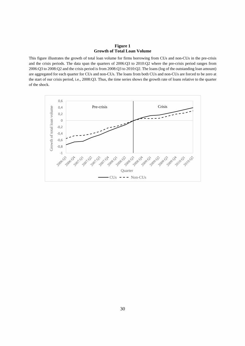
The impact of the financial crisis on bank lending in Brazil is illustrated in Figure 1. It

shows the growth of loans for CUs and non-CUs in the pre-crisis and the crisis periods, relative to

9 As a robustness check, we do the exercise using the period from 2007:Q3 to 2009:Q2 (1 year before and 1 year after the shock). Results are qualitatively unchanged and are available from the authors upon request.

10

the quarter of the shock, i.e., 2008:Q3. In the pre-crisis period, the average growth rate of loans

for CUs was 9.2%, whereas for non-CUs, it was 6.8%. The average growth rate reduced for both

groups after the shock, showing the average growth rate of 6.8% for CUs and 5.1% for non-CUs.

This implies that the growth rate reduced by 2.4 percentage points for CUs compared with the drop

of 1.7 percentage points for non-CUs. Overall, the data indicate that the crisis reduced the growth

of bank lending in Brazil.

The samples we use from the credit registry include all non-financial and private firms with

outstanding credit. Following the literature, we exclude default operations with more than 90 days,

reducing the risk that results are influenced by the carrying amount of non-paid debt in the

dependent variable. The results are robust to the inclusion of default loans.10 The sample of banks

includes CUs and non-CUs with a commercial portfolio. The data level is a triplet on the firm-

bank-quarter dimensions.

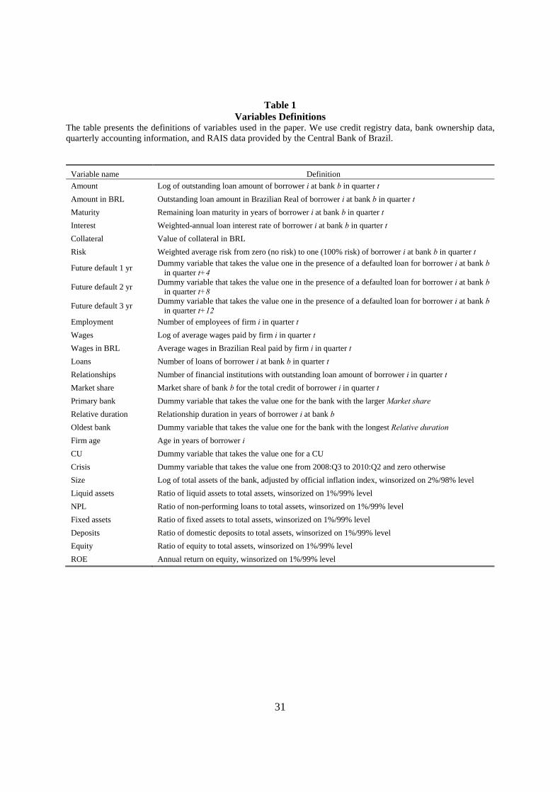
Table 1 shows the definitions of all variables used in our paper. The primary dependent

variable is Amount, defined as the natural logarithm of the total outstanding loan amount of

borrower i at bank b in quarter t. We additionally analyze the effect of the crisis on Maturity,

Interest, Collateral, Risk, and Future default to understand the multitude of possible effects on the

credit relationship of firms with CUs and non-CUs in Brazil.

We use dummy variables to indicate bank type. CU takes the value one if the financial

institution is a CU. Additionally, we have several bank-level characteristics, which include the size

of the bank, the ratio of liquid assets, fixed assets, deposits, equity, non-performing loans to total

10 In the case that a firm is in default for more than 90 days and continues in this situation, the outstanding loan amount stays the same throughout the sample period. By excluding these operations, we are able to follow the actual change in the credit supply of banks in the post-period.

11

assets, and return on equity. These controls check the robustness of our findings, i.e., whether the

inclusion of other covariates changes the results estimated in the baseline models.

To control for unobservable firm heterogeneity, we select only firms borrowing from at

least two banks at the same time. As the identification strategy relies on a comparison between the

behavior of CUs and non-CUs at the same time, we select firms that borrow from at least one CU

and one non-CU (foreign, private, domestic, or government-owned bank) in the pre-crisis and in

the crisis periods.

In other words, we apply (i) a cross-section filter, where firms must have a relationship

with a CU and a non-CU in the same quarter and (ii) a time-series filter, where relationships must

appear before and after the shock. Specifically, we investigate the impact on the intensive margin

of the same firm at the same point in time for CUs and non-CUs. The strategy of using our sample

permits a powerful identification within borrowers to disentangle features of bank’s credit supply

from firm’s credit demand.

We recognize that the restricted sample may not be representative of the population of firms

in Brazil. However, to the extent that the non-exclusivity in the banking relationship is most

controversial in the literature, the selection bias may be beneficial for our analysis. These are the

situations where the firm may have a better chance of accessing credit (if not from one bank, from

another one), and this is precisely what we want to capture in terms of credit supply and additional

credit features.

B. Firm-level Data

To study the labor market effects of the CUs’ insurance effect, we use the RAIS data

obtained from the Central Bank of Brazil. RAIS is the database of the labor market that is collected

12

annually by the Ministry of Labor and Employment (MTE). RAIS contains information on the

characteristics of the firms and their formal workers on an individual level. The data cover various

characteristics of firms and employees such as demographics, occupation, industry, income, job

starting dates, and termination dates. Firms are required by law to provide detailed information

about their employees to the MTE.

To prepare our sample, first we collapse the firm-bank-time level credit registry data on

the firm-time level. Then, we transform the annual RAIS data into quarterly RAIS data and merge

it with the credit registry data using the unique firm ID. The data are at the firm-time level. Our

sample period for labor market analysis runs from 2007:Q3 until 2010:Q2. This is a three-year

sample, one year before and two years after the shock. We cover a shorter period because the RAIS

data starts in 2007. We use the variables Employment and Wages, where Employment represents

the number of employees and Wages is the log of average wages in Brazilian Real (BRL).

For our sample of firms, the maximum number of employees is 15,294. The median

number of employees is 14, and the standard deviation is 538. The average of wages paid by the

firms is R$ 121,254, median wage is R$ 10,580 and the standard deviation is R$ 807,246. This

reflects huge variation in the data. Thus, we exclude the few large firms in the sample11. SMEs are

most relevant to our context because the CUs are an important source of finance mainly for small

businesses. The large variation in the data also leads to our decision to study the employment

effects by firm size, as in Chodorow-Reich (2014). To categorize the firms by size, we use the

OECD’s classification of SMEs. Microenterprises are firms that employ fewer than 10 employees,

11 The number of large firms is 325.

13

small firms employ 10 to 50 employees, and medium firms employ more than 50 but fewer than

250 employees. Our final merged sample has 12,694 firms and 439,211 observations.

IV. Descriptives and DD Analysis

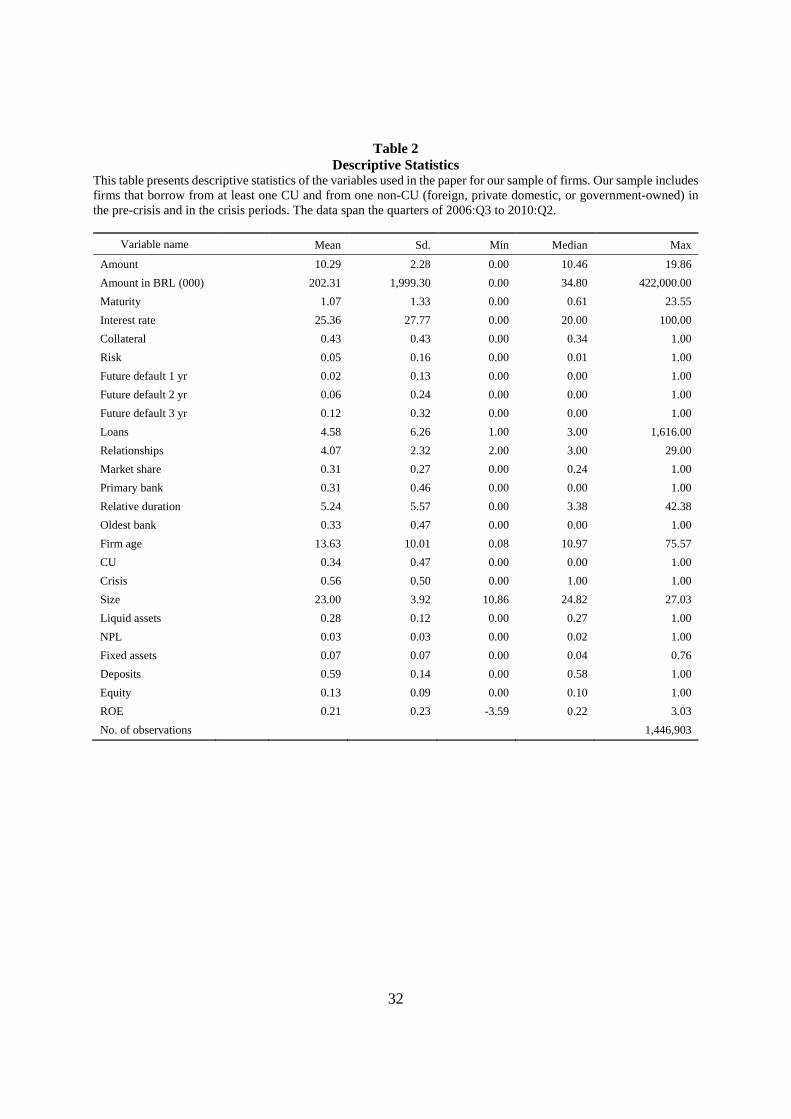
Table 2 shows summary statistics of all variables from our sample. We track 43,852 firms

and 1,001 banks that together result in 191,829 bank-firm pairs in a total of 1,446,903 observations.

The median loan amount is approximately 34,800 BRL with median remaining maturity over

seven months, median annual interest rate approximately 20% and collateral rate approximately

34%.12 On average, the future default of one year, i.e., default on a loan within four quarters, is

approximately 2%. Firms have a median of three loans with a bank and a median of three active

banking relationships, where the average market share is 31%. The median banking relationship

duration is slightly below 3.5 years, and the median firm’s age is approximately 10 years.

CUs correspond to 34% of the observations of bank-firm relationships, and 56% of the

observations are in the crisis period. The bank size in the sample is approximately 9.5 billion BRL

on average, with a balance sheet structure of 28% of their total assets invested in liquid assets and

7% in fixed assets.13 On average, non-performing loans represent 3%. The median bank has 59%

of its obligations as deposits and 13% as equity. The median bank has a net positive annual return

on assets. However, there is extreme variance in the cross-section dimension of banks’ balance

sheet structure and size. Such balance sheet differences can be correlated with credit supply, and

12 Median loan amount in USD is 18,000 on average for the period of analysis. 13 Bank size of approximately 5 billion USD on average for the period of analysis. The bank size in Table 2 is log of total assets of the bank.

14

so we formally include these variables in the regression analyses. It is important to cite that

systematic differences across banks are controlled in the regressions by bank fixed effects.

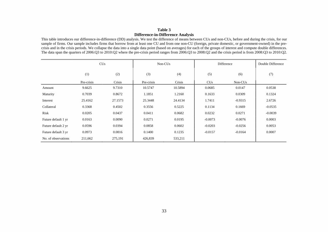
Table 3 introduces our difference-in-difference (DD) analysis. We test the difference of

means between the CUs and the non-CUs for our dependent variables in the pre-crisis and the

crisis periods. To do so, we collapse the data into a single data point (based on averages) for each

of the groups of interest and compute differences. We have 211,662 observations for CUs in the

pre-crisis period and 275,191 in the crisis period, whereas for non-CUs, there are 426,839

observations in the pre-crisis period and 533,211 in the crisis period.

For the first difference, we observe that the direction of difference for all variables is the

same for the CUs and the non-CUs except for interest rate. On average, the firms have lower

outstanding loan amount with the CUs than with the non-CUs in both the pre-crisis and the crisis

periods. However, there is an increase in the average outstanding loan amount for both groups

during the crisis period, with the increase being higher for the CUs. The change in the average

outstanding loan amount for the CUs is approximately 0.07 compared to the change of 0.01 for the

non-CUs. This is also reflected in column (7) of Table 3. The double difference of 0.05 indicates

that the CUs increased credit supply more than the non-CUs in the crisis period. It may seem odd

that both CUs and non-CUs slightly increased the average loan amount. However, this has to be

interpreted in light of the still growing market for bank loans, even though the growth rates of the

total loan amount decreased during the crisis by approximately two percentage points (see Figure

1). The growth of the average loan amount also supports this finding: CUs were increasing the

average loan amount by 0.9% on a quarterly basis in the pre-crisis period, while this growth rose

to 2% during the crisis. In contrast, the quarterly growth rate of the average loan amount decreased

from 3.2% during the pre-crisis period to 2.2% during the crisis period in the case of non-CUs.

15

The loans from the CUs have shorter remaining maturity in the pre-crisis period compared

to the non-CUs. However, the difference reduced in the crisis period, indicating that the remaining

maturity of loans from the CUs increased more in the crisis period compared to the non-CUs. This

is also evident from the double difference of 0.13 in column (7). Additionally, the CUs increased

the interest rate during the crisis, while the non-CUs decreased the interest rate. On average, the

CUs charged a slightly higher interest rate than the non-CUs before the shock, while after the

shock, they charged considerably more interest than non-CUs. The double difference indicates that

the CUs charged on average 2.67 percentage points more interest than the non-CUs in the crisis

period. The CUs required on average less collateral than the non-CUs in the pre-crisis period. In

the crisis period, even though both CUs and non-CUs required more collateral, the double

difference of -0.05 shows that the collateral requirement increased more for the non-CUs than for

the CUs.

The loans of the CUs carried lower risk in the pre-crisis period compared to the non-CUs.

The risk increased for both groups after the shock, with the increase being greater in the case of

the non-CUs’ loans. The future default rate in the first, second, and third years is lower for the CUs

than for the non-CUs both in the pre-crisis and the crisis periods. It is interesting to note that the

future default rate (in years one, two, and three) decreased after the shock for both bank groups.

This outcome should be studied in combination with the change in the amount of lending. The

CUs increased credit supply more than the non-CUs in the crisis period. However, the double

differences of all three future default measures show that there was almost no difference in the

future default rate of loans of CUs and non-CUs. The only exception is the second year, where the

decrease in future default rate was slightly lower for the CUs in the crisis period.

16

Thus, the double differences indicate that in the crisis period, the CUs supplied larger loans,

of longer maturity, and with lower collateral requirements but without any noticeable adverse

impact on the performance of the loans. Overall, the evidence so far seems to support the insurance

effect of CUs, meaning that the CUs provided insurance to their members against credit constraints

in dire times.

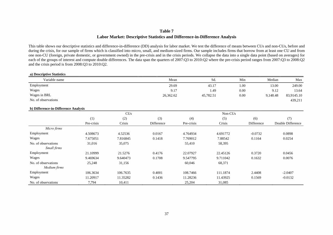
Table 7 shows summary statistics and difference-in-difference (DD) analysis for our

sample of firms from RAIS data. Panel A of Table 7 shows that, on average, the SMEs have 30

employees. The median number of employees is 13, and the standard deviation is 43. The average

of wages paid by the firms is R$ 26,363; median wage is R$ 9,148, and the standard deviation is

R$ 45,783.

In panel B, we observe that the first difference for all categories of firms is positive for

both the CUs and the non-CUs, except for Employment, which is negative for non-CUs in the case

of micro firms. For the micro firms that are borrowing from the CUs in the pre-crisis period, both

Employment and Wages increased in the crisis period. In the case of non-CUs, there is a decrease

in Employment after the shock. The Wages report a positive change of 0.12 in the crisis period.

However, this is lower than the increase in Wages in the case of CUs. The positive double

differences — 0.08 for Employment and 0.02 for Wages — indicate favorable effects on the labor

market in the form of an increase in employment and wages for the micro firms.

For the small firms, the change in our variables of interest after the shock is positive for

both CUs and non-CUs. Nonetheless, the increase is slightly more in the case of CUs, which is

reflected in the positive double differences of 0.05 and 0.01 in Employment and Wages,

respectively. For the medium firms, we notice that the firms that are borrowing from the non-CUs

before the crisis have on average 109 employees compared with 106 employees of the medium

17

firms that are borrowing from the CUs. This is also an indication that the larger firms depend more

on the non-CUs. After the shock, there is an increase in Employment and Wages of the medium-

sized firms borrowing from both the CUs and the non-CUs. However, the negative double

differences mean that the increase in Employment and Wages was higher for the firms borrowing

from the non-CUs. Overall, the results suggest that the active insurance effect of the CUs translated

into positive employment effects on micro and small firms. It seems that CUs are important to

support small firms in dire times, which in turn contributes favorably to the real economy.

V. Empirical Strategy

We use the following specification to investigate whether CUs differ with respect to

lending volume during the financial crisis compared to other banks. We will start with a

specification without any fixed effects and covariates

Yibt = α + CUb + Crisist + ßCUb*Crisist + εibt (1)

where Y represents our measures of the intensive margin, which include Amount, Maturity, Interest

or Collateral, a risk measure Risk, and measures of loan performance, i.e., Future default 1 yr,

Future default 2 yr and Future default 3 yr. In particular, Amount equals the total outstanding

credit volume of bank b towards firm i at quarter t. CU takes the value 1 if bank b is a credit union

and 0 otherwise; Crisis equals 1 from 2008:Q3 to 2010:Q2 and 0 otherwise. Overall, we expect a

negative effect of the crisis on existing firm-bank relationships, for instance, a decrease in the

outstanding loan amount, which may be driven by both credit supply and demand. Financial crisis

is a bank-level liquidity shock. Thus, changes in the loan from the same bank can be correlated.

Therefore, we cluster all errors at the bank level.

18

The principal challenge is the simultaneous nature of the bank lending channel (credit

supply) and the firm borrowing channel (credit demand). We aim to capture demand shocks at the

firm level by using firm-time fixed effects, αit, i.e., in the sense that we investigate the same firm

at the same point in time. This approach comes at the cost that we will need to constrain our

analysis to those firms with multiple bank relationships at the same time. Our most saturated

specification is thus

Yibt = αit + αib + ßCUb *Crisist + Xbt + εibt (2)

where the second set of fixed effects, αib, controls for unobserved cross-sectional heterogeneity at

the firm-bank pair level. This also includes any other time-invariant heterogeneity of credit supply

at the firm-bank level. Vector X controls for a set of observable characteristics of bank b at time t

such as the size of the bank, the ratio of liquid assets, fixed assets, deposits, capital, non-performing

loans to total assets, and return on equity. These bank characteristics are used to control for further

time-variant bank-specific determinants of credit supply.

The coefficient of interest in the specification (2), ß, is the interaction of CU with Crisis.

We want to concentrate on the financial crisis because this was a period when insurance against

credit constraints was most important to firms. If the coefficient of interest turns out to be positive,

CUs would have decreased the loan amounts to the same firm at the same point in time to a lesser

extent than other types of lenders. This case would lend support to the insurance effect. If the

coefficient of interest is negative, CUs would not have been able or willing to decrease the loan

amounts to the same firm at the same point in time to a lesser extent than other types of lenders.

This would be evidence for the equity effect. CU members can leave anytime, which would reduce

the equity of the CU. As the risk of insolvency increases during times of financial distress,

members may indeed withdraw their equity during the crisis. The coefficient of interest would

19

show whether CUs behave differently with respect to their equity ratio than other lenders.

We further test whether results depend on the banks’ equity ratio. Banks with a high equity

ratio may have been more able to maintain lending to their commercial clients, while those with

low equity ratios may have been less able to do so. We thus define a new dummy variable,

HighEquity. HighEquity equals one for CUs if a CU’s equity is above the median for all CUs at

quarter t and equals one for non-CUs if a non-CU’s equity is above the median for all non-CUs at

quarter t. Note that the equity ratio was included in vector X in specifications (1) and (2):

Yibt = αit + αib + ß1HighEquitybt + ß2CUb*Crisist + ß3HighEquitybt*Crisist +

ß4CUb*HighEquitybt + ß5CUb*Crisist*HighEquitybt + Xbt + εibt (3)

in which ß5 is the main coefficient of interest. We include firm-time and firm-bank fixed effects in

specification (3).

We extend our analysis by studying the labor market effects of the CUs’ behavior of

providing insurance to their members. We test whether the firms that had a higher share of lending

from the CUs before the crisis were able to maintain (or increase) employment during the crisis

period. We thus generate a new dummy variable, HighShare, which equals one if firms had a high

share of loans (above median) from the CUs before the crisis. We use the following specification:

Yit = αi + αt + ßHighSharei*Crisist + εit (4)

where Yit represents the dependent variables of Employment and Wages at firm-time level. The

firm and time fixed effects are captured by αi and αt, respectively. The errors, εit, are clustered at

the firm level. Specification (4) is different from our specification (2) because it studies the firm-

level outcomes for which the setup is two-dimensional, i.e., firm-time level.

20

VI. Loan Market Results

A. Intensive Margin

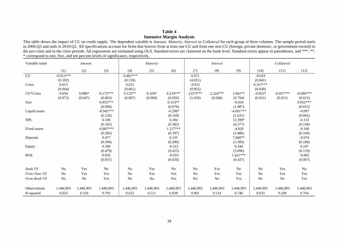
Table 4 provides the first regression results. We regress Amount, Maturity, Interest, and

Collateral on CU in the crisis period in a differences-in-differences approach. Columns (1) to (3)

show the effect of the dummy CU on the amount of credit supplied in the period from 2008:Q3 to

2010:Q2. In column (1), we do not include any type of fixed effects. The estimate of coefficient

is not statistically significant, although it is positive and economically meaningful. To address the

possibility of time-varying differences in borrower demand, we include firm-time fixed effects in

column (2). Additionally, we add bank fixed effects to control for any time-invariant bank

characteristics. In this setting, the coefficient of the interaction term becomes statistically

significant at the 10% level with an approximate 9% increase in credit supply. The last

specification of column (3) is our preferred specification because it takes into account the demand

effects and unobserved firm-bank heterogeneity. The point estimate for increases to 17.2% and

is statistically significant at the 1% level once we further include time-varying bank characteristics

and add firm-bank fixed effects instead of bank fixed effects. This result is particularly interesting

because we know that the Brazilian public banks also displayed countercyclical behavior during

the global financial crisis (IMF, 2012). Hence, we document CUs as private

mechanisms/institutions to offset the effects of financial crisis.

In columns (4) to (6), the outcome variable is Maturity. In column (4), one can observe that

the Maturity of loans granted by CUs was on average smaller than that of non-CUs (almost six

months shorter remaining maturity). However, in the crisis period, Maturity of the credit provided

by CUs increased by 48 days (0.132*365) when compared to non-CUs. Column (6) in Table 4

presents the preferred estimation. CUs increased the remaining maturity by 23 percentage points

21

compared with non-CUs. The inclusion of a set of fixed effects and time-varying bank controls in

the specification (6) makes it unlikely that the results are driven by unobservable time-varying

differences in borrower demand and quality, by time-invariant bank heterogeneity, or by time-

varying differences in the bank’s structure, behavior, or risk appetite.

Moving to columns (7) to (9), we document the effects of the financial crisis on Interest.

In the crisis period, CUs charged higher interest rates to provide credit to firms. Using our most

saturated specification, we find that CUs charged an additional interest rate of 1.7%. This is an

economically and statistically significant finding. However, this effect needs to be seen in

perspective with Brazilian basic interest rates, which were approximately 10% for the crisis period.

Furthermore, the results for interest rate need to be considered together with the collateral

requirement, the results for which are displayed in columns (10) to (12). Throughout the

specifications, we find that CUs required on average 6% less collateral in the crisis period when

compared to non-CUs. These results might corroborate the thesis that CUs would be more inclined

to take risks in a period of distress for the banking sector in Brazil.

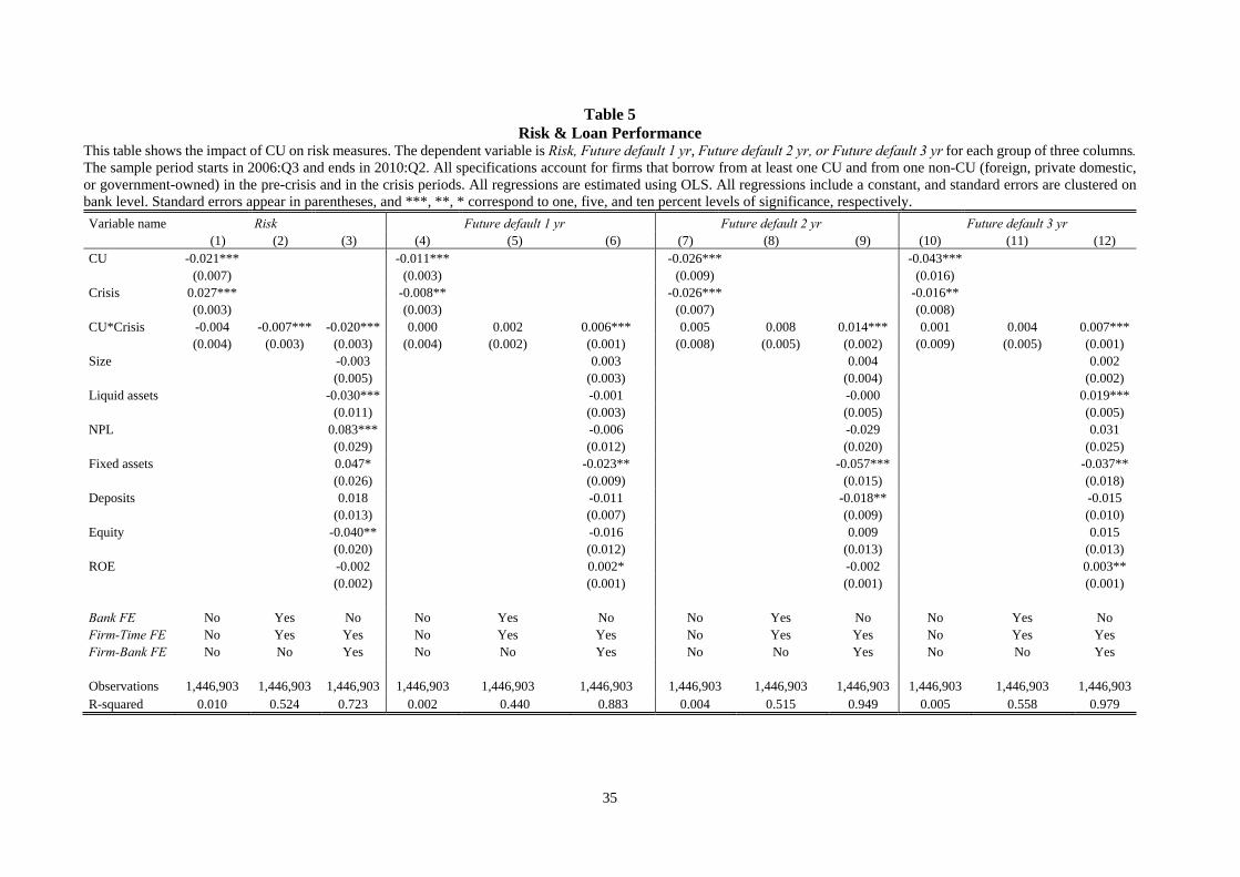
B. Risk and Loan Performance

To study whether the behavior of CUs (i.e., supplying more credit, with longer maturities,

higher interest rates, and less collateral) was translated into higher risk-taking, we test whether

Risk and Future default changed in the crisis period for CUs versus non-CUs. First, we check

whether the overall risk of the portfolio changed over time. In columns (1) to (3) of Table 5, we

use Risk, defined as the weighted average risk from zero (no risk) to one (100% risk) of borrower

i at bank b in quarter t. This variable is the same as that used by the Central Bank of Brazil to check

the provisional levels of credit portfolios of banks. It has the advantage of allowing us to check the

22

changes below and above 90 days that might not be present when we just consider the presence of

defaulted loans above 90 days. Throughout the specifications, we find that CUs did not display

higher risk on their credit portfolios when compared to non-CUs in the post period.

At this stage, one may argue that just the fact that CUs supplied more credit could explain

the lower rates of risk because new credit rises normally with higher ratings. Therefore, we also

test the performance of a loan in the next three years using Future default 1 yr, Future default 2

yr, and Future default 3 yr as dependent variables. Future default 1 yr is defined as a dummy

variable that takes the value one in the presence of a defaulted loan for borrower i at bank b in

quarter t+4. Similarly, Future default 2 yr and Future default 3 yr take the value one in the presence

of a defaulted loan for borrower i at bank b in quarters t+8 and t+12, respectively. The results are

shown in Table 5. Throughout specifications (4) to (12), we find positive results in the direction

that CUs presented higher rates of future default in the crisis period when compared to non-CUs.

The results for our most saturated specification are statistically significant. In the crisis period, the

future default rate of loans of CUs within one year is 0.6% higher compared to non-CUs. The

future default rate is 1.4% higher than non-CUs in the second year and 0.7% higher than non-CUs

in the third year. It makes sense to read these findings together with the result of Risk. Although

the risk at the time of sanctioning the loans was not higher than that of non-CUs, still the increased

supply of credit with relatively easy terms (higher maturity and less collateral) resulted in more

future costs in the form of higher default rates.

Nonetheless, the results of Table 4 and 5 present evidence of the importance of CUs in

offsetting the effect of the financial crisis of 2008. These institutions provided more credit, with

longer maturities, higher interest rates, and less collateral in the crisis period when compared to

non-CUs. However, this behavior was translated into higher credit risk.

23

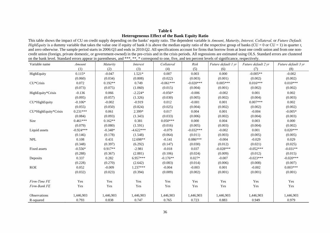
C. Heterogeneous Effects

Table 6 presents the results of our specification (3), i.e., the heterogeneous effects of the

equity ratio. Columns (1) to (8), respectively, report the effect on Amount, Maturity, Interest,

Collateral, Risk, Future default 1 yr, Future default 2 yr, and Future default 3 yr of the loans

granted by banks with high equity ratio in the period from 2008:Q3 to 2010:Q2. Column (1) shows

that the coefficient of interest for Amount is statistically significant and increases to 0.23. This

finding suggests that CUs with equity ratio above the median provided on average 23% more loans

during the crisis period compared to non-CUs. This also implies that most likely because of the

lack of capital, CUs with equity ratio below the median were not able to supply more loans in the

crisis period, i.e., were not able to provide insurance to their members.

Results in column (2), although not statistically significant, show that HighEquity CUs

provided loans of greater maturity compared to non-CUs during the crisis. Moving to column (3),

we find that the interest rate charged by HighEquity CUs increased during the crisis. The CUs with

equity ratio above median charged on average 2.4% higher interest rate than non-CUs. In columns

(4) to (7), we do not generally observe any significant impact on the coefficients of interest. In

column (8), we have a statistically significant finding at the 10% level, indicating that in the next

three years, CUs with above median equity ratio faced 0.5% fewer defaults than non-CUs. Overall,

the findings of specification (3) support the insurance effect observed in our specification (2). We

thus conclude that the insurance effect seems to dominate the equity effect.14

14 Our loan market results remain qualitatively unchanged if we divide the firms by size into micro, small, and medium firms.

24

VII. Labor Market Effects

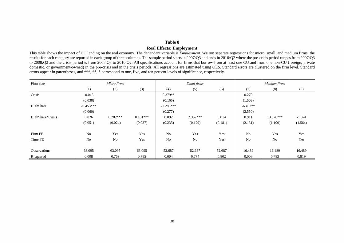
Table 8 presents the results for Employment. Columns (1) to (3) report the effect of the

dummy HighShare on Employment level of the micro firms in the crisis period. Columns (4) to (6)

report the same for the small firms, and columns (7) to (9) show the results for the medium firms.

In column (3), which is our most saturated specification for micro firms, the coefficient of interest

for Employment is statistically significant at the 1% level. The positive value of 0.1 shows that the

micro firms that had above-median loans from the CUs in the pre-crisis period were able to hire

on average 10% of an employee during the crisis period. Alternatively, this result can also be

interpreted to mean that at least one in ten firms hired one more employee during the crisis period.

For the small firms, the positive point estimate for β in column (6), although not significant,

indicates positive employment outcomes. For the medium firms, the coefficient in column (8)

indicates strong positive effects on employment. However, the results lose significance, and the

coefficient turns negative when we include both firm and time fixed effects in column (9).

Table 9 reports the effect of the dummy HighShare on Wages paid by the firms in the crisis

period. As in Table (8), columns (1) to (3) report the results for micro firms, columns (4) to (6) for

the small firms, and columns (7) to (9) for the medium firms. For micro firms, column (3) reports

statistically significant results at the 5% level. The estimate for β shows that the micro firms that

had above-median loans from the CUs before the crisis provided on average 3% more wages

during the crisis period. The effect on wages paid by the small and medium firms is positive and

significant in columns (5) and (7). However, for our most saturated specification in columns (6)

25

and (9), the results lose significance and report slightly negative estimates.15

The higher dependence of micro and small firms on CUs is also evident from the number

of observations for each group of firms in Tables 8 and 9. In our sample of firms that borrow from

both the CUs and the non-CUs, micro firms make the biggest proportion of observations, i.e.,

63,095, whereas the number of observations for the medium firms is roughly only 25% of the

micro firms. Thus, the findings of our paper suggest that the CUs support their members by easing

credit constraints during dire times. Further, the active insurance effect of the CUs translates into

positive effects on the real economy in the form of an increase in employment and wages among

the micro and small firms.

VIII. Conclusions

In this paper, we analyze the lending behavior of CUs as prototypical relationship lenders

and the subsequent effects on the borrowing firms’ labor force during the financial crisis of

2008/09. Our results imply that during the crisis, Brazilian CUs tighten credit to borrowers less

than other bank types (insurance effect). This outcome is consistent with the insurance hypothesis

that CUs, compared to other banks, try harder to support their borrowers during dire times. CU

members enjoyed longer maturity loans and less collateral requirement. However, CU members

were paying higher interest rates for this type of insurance, and CUs faced higher future default

frequencies. We further provide empirical evidence on the labor market outcome of the CUs’

insurance effect. The insurance effect of CUs transmitted to more employment and higher wages

15 We estimated our labor market results using another sample of RAIS data that also includes firms with 0 employees (self-employed). However, these data are annual and not well-suited for our research design. Nonetheless, our labor market results remain qualitatively unchanged.

26

for very small firms. Overall, CUs appear to be able to prevent the propagation of negative shocks

of the financial crisis because of their non-procyclical behavior during the crisis.

27

References

Albertazzi, Ugo, and Domenico Junior Marchetti. "Credit Supply, Flight to Quality and

Evergreening: An Analysis of Bank-firm Relationships after Lehman." Working Paper No. 756.

Bank of Italy, 2010.

Angelini, Paolo, Roberto Di Salvo, and Giovanni Ferri. "Availability and Cost of Credit for Small

Businesses: Customer Relationships and Credit Cooperatives.” Journal of Banking & Finance 22

(1998): 925-954.

Bayoumi, Tamim, and Gabrielle Lipworth. "Japanese Foreign Direct Investment and Regional

Trade." Journal of Asian Economics 9 (1999): 581-607.

Benmelech, Efraim, Nittai K. Bergman, and Amit Seru. Financing Labor. Working Paper No.

w17144. National Bureau of Economic Research, 2011.

Berlin, Mitchell, and Loretta J. Mester. "On the Profitability and Cost of Relationship Lending."

Journal of Banking & Finance 22 (1998): 873-897.

Chava, Sudheer, and Amiyatosh Purnanandam. "The Effect of Banking Crisis on Bank-dependent

Borrowers." Journal of Financial Economics 99 (2011): 116-135.

Chodorow-Reich, Gabriel. “The Employment Effects of Credit Market Disruptions: Firm-level

Evidence from the 2008-9 Financial Crisis.” Quarterly Journal of Economics 129 (2014): 1-59.

Cole, Rebel A. "The Importance of Relationships to the Availability of Credit." Journal of Banking

& Finance 22 (1998): 959-977.

28

Coleman, Nicholas, and Leo Feler. "Bank Ownership, Lending, and Local Economic Performance

during the 2008–2009 Financial Crisis." Journal of Monetary Economics 71 (2015): 50-66.

Elsas, Ralf, and Jan Pieter Krahnen. "Is Relationship Lending Special? Evidence from Credit-file

Data in Germany." Journal of Banking & Finance 22 (1998): 1283-1316.

Ferri, Giovanni, and Marcello Messori. "Bank–firm Relationships and Allocative Efficiency in

Northeastern and Central Italy and in the South." Journal of Banking & Finance 24 (2000): 1067-

1095.

Hackethal, Andreas. “German Banks and Banking Structure”. Working Paper No. 106.

Department of Finance, Goethe University Frankfurt am Main, 2004.

Hoshi, Takeo, Anil Kashyap, and David Scharfstein. “The Role of Banks in Reducing the Costs

of Financial Distress in Japan.” Journal of Financial Economics 27 (1990): 67-88.

Iyer, Rajkamal, José-Luis Peydró, Samuel da-Rocha-Lopes, and Antoinette Schoar. "Interbank

Liquidity Crunch and the Firm Credit Crunch: Evidence from the 2007–2009 Crisis." Review of

Financial Studies 27, No. 1 (2013): 347-372.

Jiménez, Gabriel, and Steven Ongena. "Credit Supply and Monetary Policy: Identifying the Bank

Balance-sheet Channel with Loan Applications." American Economic Review 102 (2012): 2301-

2326.

Jiménez, Gabriel, Steven Ongena, José‐Luis Peydró, and Jesús Saurina. "Hazardous Times for

Monetary Policy: What Do Twenty‐Three Million Bank Loans Say About the Effects of Monetary

Policy on Credit Risk‐Taking?" Econometrica 82 (2014): 463-505.

29

Khwaja, Asim Ijaz, and Atif Mian. “Tracing the Impact of Bank Liquidity Shocks: Evidence from

an Emerging Market.” American Economic Review 98 (2008): 1413-1442.

Machauer, Achim, and Martin Weber. “Number of Bank Relationships: An Indicator of

Competition, Borrower Quality, or just Size?” Working Paper No. 2000/06. Goethe-Universität

Center for Financial Studies, 2000.

Mian, Atif. "Distance Constraints: The Limits of Foreign Lending in Poor Economies." Journal of

Finance 61 (2006): 1465-1505.

Morck, Randall, Masao Nakamura, and Murray Frank. "Japanese Corporate Governance and

Macroeconomic Problems." In The Japanese Business and Economic System, 325-363. Palgrave

Macmillan UK, 2001.

Paravisini, Daniel. "Local Bank Financial Constraints and Firm Access to External

Finance." Journal of Finance 63 (2008): 2161-2193.

Peek, Joe, and Eric S. Rosengren. "The International Transmission of Financial Shocks: The Case

of Japan." American Economic Review 87 (1997): 495-505.

Petersen, Mitchell A., and Raghuram G. Rajan. "The Benefits of Lending Relationships: Evidence

from Small Business Data." Journal of Finance 49 (1994): 3-37.

Schnabl, Philipp. "The International Transmission of Bank Liquidity Shocks: Evidence from an

Emerging Market.” Journal of Finance 67 (2012): 897-932.

Wagner, Wolf. "Systemic Liquidation Risk and the Diversity–Diversification Trade-Off." Journal

of Finance 66 (2011): 1141–1175.

30

Figure 1 Growth of Total Loan Volume

This figure illustrates the growth of total loan volume for firms borrowing from CUs and non-CUs in the pre-crisis and the crisis periods. The data span the quarters of 2006:Q3 to 2010:Q2 where the pre-crisis period ranges from 2006:Q3 to 2008:Q2 and the crisis period is from 2008:Q3 to 2010:Q2. The loans (log of the outstanding loan amount) are aggregated for each quarter for CUs and non-CUs. The loans from both CUs and non-CUs are forced to be zero at the start of our crisis period, i.e., 2008:Q3. Thus, the time series shows the growth rate of loans relative to the quarter of the shock.

‐1

‐0,8

‐0,6

‐0,4

‐0,2

0

0,2

0,4

0,6

Gro

wth

of

tota

l loa

n vo

lum

e

Quarter

CUs Non-CUs

Pre-crisis Crisis

31

Table 1 Variables Definitions

The table presents the definitions of variables used in the paper. We use credit registry data, bank ownership data, quarterly accounting information, and RAIS data provided by the Central Bank of Brazil.

Variable name Definition

Amount Log of outstanding loan amount of borrower i at bank b in quarter t

Amount in BRL Outstanding loan amount in Brazilian Real of borrower i at bank b in quarter t

Maturity Remaining loan maturity in years of borrower i at bank b in quarter t

Interest Weighted-annual loan interest rate of borrower i at bank b in quarter t

Collateral Value of collateral in BRL

Risk Weighted average risk from zero (no risk) to one (100% risk) of borrower i at bank b in quarter t

Future default 1 yr Dummy variable that takes the value one in the presence of a defaulted loan for borrower i at bank b

in quarter t+4


in quarter t+8


in quarter t+12 Employment Number of employees of firm i in quarter t

Wages Log of average wages paid by firm i in quarter t

Wages in BRL Average wages in Brazilian Real paid by firm i in quarter t

Loans Number of loans of borrower i at bank b in quarter t

Relationships Number of financial institutions with outstanding loan amount of borrower i in quarter t

Market share Market share of bank b for the total credit of borrower i in quarter t

Primary bank Dummy variable that takes the value one for the bank with the larger Market share

Relative duration Relationship duration in years of borrower i at bank b

Oldest bank Dummy variable that takes the value one for the bank with the longest Relative duration

Firm age Age in years of borrower i

CU Dummy variable that takes the value one for a CU

Crisis Dummy variable that takes the value one from 2008:Q3 to 2010:Q2 and zero otherwise

Size Log of total assets of the bank, adjusted by official inflation index, winsorized on 2%/98% level

Liquid assets Ratio of liquid assets to total assets, winsorized on 1%/99% level

NPL Ratio of non-performing loans to total assets, winsorized on 1%/99% level

Fixed assets Ratio of fixed assets to total assets, winsorized on 1%/99% level

Deposits Ratio of domestic deposits to total assets, winsorized on 1%/99% level

Equity Ratio of equity to total assets, winsorized on 1%/99% level

ROE Annual return on equity, winsorized on 1%/99% level

32

Table 2

Descriptive Statistics This table presents descriptive statistics of the variables used in the paper for our sample of firms. Our sample includes firms that borrow from at least one CU and from one non-CU (foreign, private domestic, or government-owned) in the pre-crisis and in the crisis periods. The data span the quarters of 2006:Q3 to 2010:Q2.

Variable name Mean Sd. Min Median Max

Amount 10.29 2.28 0.00 10.46 19.86

Amount in BRL (000) 202.31 1,999.30 0.00 34.80 422,000.00

Maturity 1.07 1.33 0.00 0.61 23.55

Interest rate 25.36 27.77 0.00 20.00 100.00

Collateral 0.43 0.43 0.00 0.34 1.00

Risk 0.05 0.16 0.00 0.01 1.00

Future default 1 yr 0.02 0.13 0.00 0.00 1.00



Loans 4.58 6.26 1.00 3.00 1,616.00

Relationships 4.07 2.32 2.00 3.00 29.00

Market share 0.31 0.27 0.00 0.24 1.00

Primary bank 0.31 0.46 0.00 0.00 1.00

Relative duration 5.24 5.57 0.00 3.38 42.38

Oldest bank 0.33 0.47 0.00 0.00 1.00

Firm age 13.63 10.01 0.08 10.97 75.57

CU 0.34 0.47 0.00 0.00 1.00

Crisis 0.56 0.50 0.00 1.00 1.00

Size 23.00 3.92 10.86 24.82 27.03

Liquid assets 0.28 0.12 0.00 0.27 1.00

NPL 0.03 0.03 0.00 0.02 1.00

Fixed assets 0.07 0.07 0.00 0.04 0.76

Deposits 0.59 0.14 0.00 0.58 1.00

Equity 0.13 0.09 0.00 0.10 1.00

ROE 0.21 0.23 -3.59 0.22 3.03

No. of observations 1,446,903

33

Table 3

Difference-in-Difference Analysis This table introduces our difference-in-difference (DD) analysis. We test the difference of means between CUs and non-CUs, before and during the crisis, for our sample of firms. Our sample includes firms that borrow from at least one CU and from one non-CU (foreign, private domestic, or government-owned) in the pre-crisis and in the crisis periods. We collapse the data into a single data point (based on averages) for each of the groups of interest and compute double differences. The data span the quarters of 2006:Q3 to 2010:Q2 where the pre-crisis period ranges from 2006:Q3 to 2008:Q2 and the crisis period is from 2008:Q3 to 2010:Q2.

CUs Non-CUs Difference Double Difference

(1) (2) (3) (4) (5) (6) (7)

Pre-crisis Crisis Pre-crisis Crisis CUs Non-CUs

Amount 9.6625 9.7310 10.5747 10.5894 0.0685 0.0147 0.0538

Maturity 0.7039 0.8672 1.1851 1.2160 0.1633 0.0309 0.1324

Interest 25.4162 27.1573 25.3448 24.4134 1.7411 -0.9315 2.6726

Collateral 0.3368 0.4502 0.3556 0.5225 0.1134 0.1669 -0.0535

Risk 0.0205 0.0437 0.0411 0.0682 0.0232 0.0271 -0.0039

Future default 1 yr 0.0163 0.0090 0.0271 0.0195 -0.0073 -0.0076 0.0003



No. of observations 211,662 275,191 426,839 533,211

34

Table 4

Intensive Margin Analysis This table shows the impact of CU on credit supply. The dependent variable is Amount, Maturity, Interest or Collateral for each group of three columns. The sample period starts in 2006:Q3 and ends in 2010:Q2. All specifications account for firms that borrow from at least one CU and from one non-CU (foreign, private domestic, or government-owned) in the pre-crisis and in the crisis periods. All regressions are estimated using OLS. Standard errors are clustered on the bank level. Standard errors appear in parentheses, and ***, **, * correspond to one, five, and ten percent levels of significance, respectively.

Variable name Amount Maturity Interest Collateral

(1) (2) (3) (4) (5) (6) (7) (8) (9) (10) (11) (12)

CU -0.912*** -0.481*** 0.071 -0.019 (0.102) (0.150) (4.051) (0.041) Crisis 0.015 0.031 -0.931 0.167*** (0.064) (0.061) (0.955) (0.030) CU*Crisis 0.054 0.086* 0.172*** 0.132** 0.104* 0.234*** 2.673*** 2.224*** 1.661** -0.053* -0.057*** -0.060*** (0.073) (0.047) (0.063) (0.067) (0.060) (0.050) (1.050) (0.646) (0.794) (0.031) (0.021) (0.015) Size 0.455*** 0.153** -0.034 0.052*** (0.094) (0.076) (1.887) (0.015) Liquid assets -0.942*** -0.298* -4.691*** -0.097 (0.135) (0.169) (1.631) (0.062) NPL 0.100 0.394 12.399* -0.131 (0.345) (0.382) (6.577) (0.149) Fixed assets -0.807*** 1.127*** -4.920 -0.166 (0.285) (0.397) (3.486) (0.104) Deposits 0.477 0.135 7.668** -0.074 (0.304) (0.286) (3.385) (0.106) Equity 0.399 -0.315 0.344 0.187 (0.479) (0.425) (5.096) (0.119) ROE 0.056 -0.010 1.421*** -0.002 (0.037) (0.026) (0.437) (0.007) Bank FE No Yes No No Yes No No Yes No No Yes No Firm-Time FE No Yes Yes No Yes Yes No Yes Yes No Yes Yes Firm-Bank FE No No Yes No No Yes No No Yes No No Yes

Observations 1,446,903 1,446,903 1,446,903 1,446,903 1,446,903 1,446,903 1,446,903 1,446,903 1,446,903 1,446,903 1,446,903 1,446,903 R-squared 0.033 0.559 0.793 0.022 0.511 0.838 0.001 0.514 0.746 0.033 0.549 0.764

35

Table 5

Risk & Loan Performance This table shows the impact of CU on risk measures. The dependent variable is Risk, Future default 1 yr, Future default 2 yr, or Future default 3 yr for each group of three columns. The sample period starts in 2006:Q3 and ends in 2010:Q2. All specifications account for firms that borrow from at least one CU and from one non-CU (foreign, private domestic, or government-owned) in the pre-crisis and in the crisis periods. All regressions are estimated using OLS. All regressions include a constant, and standard errors are clustered on bank level. Standard errors appear in parentheses, and ***, **, * correspond to one, five, and ten percent levels of significance, respectively.

Variable name Risk Future default 1 yr Future default 2 yr Future default 3 yr (1) (2) (3) (4) (5) (6) (7) (8) (9) (10) (11) (12) CU -0.021*** -0.011*** -0.026*** -0.043***

(0.007) (0.003) (0.009) (0.016) Crisis 0.027*** -0.008** -0.026*** -0.016**

(0.003) (0.003) (0.007) (0.008) CU*Crisis -0.004 -0.007*** -0.020*** 0.000 0.002 0.006*** 0.005 0.008 0.014*** 0.001 0.004 0.007***

(0.004) (0.003) (0.003) (0.004) (0.002) (0.001) (0.008) (0.005) (0.002) (0.009) (0.005) (0.001) Size -0.003 0.003 0.004 0.002

(0.005) (0.003) (0.004) (0.002) Liquid assets -0.030*** -0.001 -0.000 0.019***

(0.011) (0.003) (0.005) (0.005) NPL 0.083*** -0.006 -0.029 0.031

(0.029) (0.012) (0.020) (0.025) Fixed assets 0.047* -0.023** -0.057*** -0.037**

(0.026) (0.009) (0.015) (0.018) Deposits 0.018 -0.011 -0.018** -0.015

(0.013) (0.007) (0.009) (0.010) Equity -0.040** -0.016 0.009 0.015

(0.020) (0.012) (0.013) (0.013) ROE -0.002 0.002* -0.002 0.003**

(0.002) (0.001) (0.001) (0.001)

Bank FE No Yes No No Yes No No Yes No No Yes No Firm-Time FE No Yes Yes No Yes Yes No Yes Yes No Yes Yes Firm-Bank FE No No Yes No No Yes No No Yes No No Yes

Observations 1,446,903 1,446,903 1,446,903 1,446,903 1,446,903 1,446,903 1,446,903 1,446,903 1,446,903 1,446,903 1,446,903 1,446,903 R-squared 0.010 0.524 0.723 0.002 0.440 0.883 0.004 0.515 0.949 0.005 0.558 0.979

36

Table 6 Heterogeneous Effect of the Bank Equity Ratio

This table shows the impact of CU on credit supply depending on the banks’ equity ratio. The dependent variable is Amount, Maturity, Interest, Collateral, or Future Default. HighEquity is a dummy variable that takes the value one if equity of bank b is above the median equity ratio of the respective group of banks (CU = 0 or CU = 1) in quarter t, and zero otherwise. The sample period starts in 2006:Q3 and ends in 2010:Q2. All specifications account for firms that borrow from at least one credit union and from one non-credit union (foreign, private domestic, or government-owned) in the pre-crisis and in the crisis periods. All regressions are estimated using OLS. Standard errors are clustered on the bank level. Standard errors appear in parentheses, and ***, **, * correspond to one, five, and ten percent levels of significance, respectively.

Variable name Amount Maturity Interest Collateral Risk Future default 1 yr Future default 2 yr Future default 3 yr (1) (2) (3) (4) (5) (6) (7) (8) HighEquity 0.115* -0.047 1.521* 0.007 0.003 0.000 -0.005** -0.002

(0.060) (0.034) (0.808) (0.022) (0.003) (0.001) (0.002) (0.002) CU*Crisis 0.072 0.192** 0.749 -0.061*** -0.020*** 0.005*** 0.016*** 0.010***

(0.073) (0.075) (1.060) (0.015) (0.004) (0.001) (0.002) (0.002)

HighEquity*Crisis -0.136 0.066 -2.224* -0.056* -0.006 -0.002 0.001 0.002 (0.095) (0.057) (1.326) (0.030) (0.005) (0.002) (0.004) (0.003)

CU*HighEquity -0.106* -0.002 -0.919 0.012 -0.001 0.001 0.007*** 0.002 (0.055) (0.050) (0.824) (0.025) (0.004) (0.002) (0.002) (0.002)

CU*HighEquity*Crisis 0.231*** 0.061 2.399* 0.017 0.004 0.001 -0.004 -0.005* (0.084) (0.093) (1.343) (0.033) (0.006) (0.002) (0.004) (0.003)

Size 0.461*** 0.162** 0.381 0.050*** 0.000 0.004 0.003 0.000 (0.079) (0.080) (1.591) (0.016) (0.005) (0.003) (0.004) (0.002)

Liquid assets -0.924*** -0.348* -4.622*** -0.079 -0.032*** -0.002 0.001 0.020*** (0.146) (0.178) (1.548) (0.064) (0.011) (0.003) (0.005) (0.005)

NPL 0.108 0.431 12.698** -0.141 0.086*** -0.004 -0.029 0.029 (0.348) (0.397) (6.292) (0.147) (0.030) (0.012) (0.021) (0.025)

Fixed assets -0.556* 0.917** -2.981 -0.018 0.037 -0.028*** -0.052*** -0.031** (0.288) (0.367) (2.881) (0.106) (0.024) (0.009) (0.012) (0.015)

Deposits 0.337 0.282 6.957*** -0.176** 0.027* -0.007 -0.023*** -0.020*** (0.228) (0.270) (2.642) (0.083) (0.014) (0.006) (0.008) (0.007)

ROE 0.052 -0.009 1.237*** -0.004 -0.003 0.001 -0.002 0.003*** (0.032) (0.023) (0.394) (0.009) (0.002) (0.001) (0.001) (0.001)

Firm-Time FE Yes Yes Yes Yes Yes Yes Yes Yes Firm-Bank FE Yes Yes Yes Yes Yes Yes Yes Yes

Observations 1,446,903 1,446,903 1,446,903 1,446,903 1,446,903 1,446,903 1,446,903 1,446,903 R-squared 0.793 0.838 0.747 0.765 0.723 0.883 0.949 0.979

37

Table 7 Labor Market: Descriptive Statistics and Difference-in-Difference Analysis

This table shows our descriptive statistics and difference-in-difference (DD) analysis for labor market. We test the difference of means between CUs and non-CUs, before and during the crisis, for our sample of firms which is classified into micro, small, and medium-sized firms. Our sample includes firms that borrow from at least one CU and from one non-CU (foreign, private domestic, or government owned) in the pre-crisis and in the crisis periods. We collapse the data into a single data point (based on averages) for each of the groups of interest and compute double differences. The data span the quarters of 2007:Q3 to 2010:Q2 where the pre-crisis period ranges from 2007:Q3 to 2008:Q2 and the crisis period is from 2008:Q3 to 2010:Q2. a) Descriptive Statistics

Variable name Mean Sd. Min Median Max

Employment 29.69 43.17 1.00 13.00 249.00 Wages 9.17 1.49 0.00 9.12 13.64 Wages in BRL 26,362.62 45,782.51 0.00 9,148.48 83,9145.10 No. of observations 439,211 b) Difference-in-Difference Analysis CUs Non-CUs

(1) (2) (3) (4) (5) (6) (7) Pre-crisis Crisis Difference Pre-crisis Crisis Difference Double Difference

Micro firms Employment 4.508673 4.52536 0.0167 4.764934 4.691772 -0.0732 0.0898 Wages 7.675051 7.816845 0.1418 7.769012 7.88542 0.1164 0.0254 No. of observations 31,016 35,075 55,410 58,395

Small firms Employment 21.10999 21.5276 0.4176 22.07927 22.45126 0.3720 0.0456 Wages 9.469634 9.640473 0.1708 9.547795 9.711042 0.1632 0.0076 No. of observations 25,248 31,156 60,046 68,371

Medium firms Employment 106.3634 106.7635 0.4001 108.7466 111.1874 2.4408 -2.0407 Wages 11.20917 11.35282 0.1436 11.28236 11.43925 0.1569 -0.0132 No. of observations 7,794 10,411 25,204 31,085

38

Table 8 Real Effects: Employment

This table shows the impact of CU lending on the real economy. The dependent variable is Employment. We run separate regressions for micro, small, and medium firms; the results for each category are reported in each group of three columns. The sample period starts in 2007:Q3 and ends in 2010:Q2 where the pre-crisis period ranges from 2007:Q3 to 2008:Q2 and the crisis period is from 2008:Q3 to 2010:Q2. All specifications account for firms that borrow from at least one CU and from one non-CU (foreign, private domestic, or government-owned) in the pre-crisis and in the crisis periods. All regressions are estimated using OLS. Standard errors are clustered on the firm level. Standard errors appear in parentheses, and ***, **, * correspond to one, five, and ten percent levels of significance, respectively.

Firm size Micro firms Small firms Medium firms

(1) (2) (3) (4) (5) (6) (7) (8) (9)

Crisis -0.013 0.379** 0.279

(0.038) (0.165) (1.509)

HighShare -0.453*** -1.283*** -6.493**

(0.060) (0.277) (2.550)

HighShare*Crisis 0.026 0.282*** 0.101*** 0.092 2.357*** 0.014 0.911 13.976*** -1.874

(0.051) (0.024) (0.037) (0.235) (0.129) (0.181) (2.131) (1.100) (1.564)

Firm FE No Yes Yes No Yes Yes No Yes Yes

Time FE No No Yes No No Yes No No Yes

Observations 63,095 63,095 63,095 52,687 52,687 52,687 16,489 16,489 16,489

R-squared 0.008 0.769 0.785 0.004 0.774 0.802 0.003 0.783 0.819

39

Table 9 Real Effects: Wages

This table shows the impact of CU lending on the real economy. The dependent variable is Employment. We run separate regressions for micro, small, and medium firms; the results for each category are reported in each group of three columns. The sample period starts in 2007:Q3 and ends in 2010:Q2 where the pre-crisis period ranges from 2007:Q3 to 2008:Q2 and the crisis period is from 2008:Q3 to 2010:Q2. All specifications account for firms that borrow from at least one CU and from one non-CU (foreign, private domestic, or government owned) in the pre-crisis and in the crisis periods. All regressions are estimated using OLS. Standard errors are clustered on the firm level. Standard errors appear in parentheses, and ***, **, * correspond to one, five, and ten percent levels of significance, respectively.

Firm size Micro firms Small firms Medium firms

(1) (2) (3) (4) (5) (6) (7) (8) (9)

Crisis 0.143*** 0.171*** 0.139***

(0.013) (0.009) (0.017)

HighShare -0.134*** -0.077*** -0.103***

(0.021) (0.017) (0.031)

HighShare*Crisis -0.007 0.212*** 0.032** -0.001 0.256*** -0.003 0.016 0.277*** -0.012

(0.018) (0.010) (0.015) (0.013) (0.007) (0.009) (0.024) (0.010) (0.015)

Firm FE No Yes Yes No Yes Yes No Yes Yes

Time FE No No Yes No No Yes No No Yes

Observations 63,095 63,095 63,095 52,687 52,687 52,687 16,489 16,489 16,489

R-squared 0.011 0.745 0.753 0.024 0.823 0.855 0.022 0.849 0.892

Documents

Do firms benefit from their relationships with credit ... · Do firms benefit from their relationships with credit unions ... by disentangling bank credit supply ... the banking relationship