Embed Size (px)
Citation preview
Bank of Canada Banque du Canada
Working Paper 2004-49/ Document de travail 2004-49
Trade Credit and Credit Rationingin Canadian Firms
by
Rose Cunningham

ISSN 1192-5434
Printed in Canada on recycled paper

Bank of Canada Working Paper 2004-49
December 2004
Trade Credit and Credit Rationingin Canadian Firms
by
Rose Cunningham
International DepartmentBank of Canada
Ottawa, Ontario, Canada K1A [email protected]
The views expressed in this paper are those of the author.No responsibility for them should be attributed to the Bank of Canada.

iii
Contents
Acknowledgements. . . . . . . . . . . . . . . . . . . . . . . . . . . . . . . . . . . . . . . . . . . . . . . . . . . . . . . . . . . . ivAbstract/Résumé . . . . . . . . . . . . . . . . . . . . . . . . . . . . . . . . . . . . . . . . . . . . . . . . . . . . . . . . . . . . . . v
1. Introduction . . . . . . . . . . . . . . . . . . . . . . . . . . . . . . . . . . . . . . . . . . . . . . . . . . . . . . . . . . . . . . 1
2. Trade Credit Literature . . . . . . . . . . . . . . . . . . . . . . . . . . . . . . . . . . . . . . . . . . . . . . . . . . . . . 2
2.1 Financial theories of trade credit . . . . . . . . . . . . . . . . . . . . . . . . . . . . . . . . . . . . . . . . . 22.2 Empirical findings on financial motives for trade credit . . . . . . . . . . . . . . . . . . . . . . . 4
3. Theoretical Framework . . . . . . . . . . . . . . . . . . . . . . . . . . . . . . . . . . . . . . . . . . . . . . . . . . . .5
3.1 Model description . . . . . . . . . . . . . . . . . . . . . . . . . . . . . . . . . . . . . . . . . . . . . . . . . . . . 53.2 Testable hypotheses . . . . . . . . . . . . . . . . . . . . . . . . . . . . . . . . . . . . . . . . . . . . . . . . . . . 7
4. Data and Summary Statistics . . . . . . . . . . . . . . . . . . . . . . . . . . . . . . . . . . . . . . . . . . . . . . . . 8
5. Estimation Method . . . . . . . . . . . . . . . . . . . . . . . . . . . . . . . . . . . . . . . . . . . . . . . . . . . . . . . 10
5.1 Estimation of trade credit usage . . . . . . . . . . . . . . . . . . . . . . . . . . . . . . . . . . . . . . . . . 105.2 Estimation of trade credit supplied and net trade credit . . . . . . . . . . . . . . . . . . . . . . 125.3 Sample splitting and estimating wealth category thresholds . . . . . . . . . . . . . . . . . . . 13
6. Regression Results . . . . . . . . . . . . . . . . . . . . . . . . . . . . . . . . . . . . . . . . . . . . . . . . . . . . . . . 14
6.1 Regression results for trade credit usage (AP/SALES) . . . . . . . . . . . . . . . . . . . . . . . . 146.2 Regression results for trade credit supplied and net trade credit . . . . . . . . . . . . . . . . 166.3 Robustness tests . . . . . . . . . . . . . . . . . . . . . . . . . . . . . . . . . . . . . . . . . . . . . . . . . . . . . 17
7. Conclusions . . . . . . . . . . . . . . . . . . . . . . . . . . . . . . . . . . . . . . . . . . . . . . . . . . . . . . . . . . . . . 18
References . . . . . . . . . . . . . . . . . . . . . . . . . . . . . . . . . . . . . . . . . . . . . . . . . . . . . . . . . . . . . . . . . . 20
Tables . . . . . . . . . . . . . . . . . . . . . . . . . . . . . . . . . . . . . . . . . . . . . . . . . . . . . . . . . . . . . . . . . . . . . . 21
Appendix: Definitions of Variables and Data Description. . . . . . . . . . . . . . . . . . . . . . . . . . . . . . 28

iv
Acknowledgements
I thank Robert Lafrance, Eric Santor, Larry Schembri, Jean-Francois Perrault, James Powell,
John Baldwin, Paul Warren, Des Beckstead, seminar participants at the Bank of Canada and
Statistics Canada, and an anonymous reviewer at Statistics Canada for helpful comments. I am
very grateful to the Microeconomic Analysis Division of Statistics Canada for providing access to
the data and supporting this research through their Ph.D. Stipend program.
v
Abstract
Burkart and Ellingsen’s (2004) model of trade credit and bank credit rationing predicts that tradecredit will be used by medium-wealth and low-wealth firms to help ease bank credit rationing.The author tests these and other predictions of Burkart and Ellingsen’s model using a large sampleof more than 28,000 Canadian firms. She uses an endogenous method to divide the firms into theappropriate wealth categories, rather than arbitrarily selecting firms likely to be credit rationed.The data support the main predictions of Burkart and Ellingsen’s model quite well. The authorfinds that medium-wealth firms substitute trade credit for bank credit consistent with using it toalleviate bank credit rationing. The low-wealth firms use trade credit, but it is positively linked totheir bank credit, which suggests that those firms are constrained in both bank credit and tradecredit markets, and so cannot use trade credit to adjust as much to negative shocks. The findingsalso suggest that there are very few unconstrained, high-wealth Canadian firms. The author alsofinds that low-wealth, declining, and distressed firms supply proportionally more trade credit thanfirms that have healthier balance sheets. This is surprising, but has been found in earlier studies aswell. It may reflect some exploitation of market power by the customers of such firms.
JEL classification: G32, G14, G21Bank classification: Financial markets; Credit and credit aggregates
Résumé
D’après le modèle de Burkart et Ellingsen (2004), les entreprises à faible ou moyenne rentabilitéauraient recours au crédit fournisseur pour compenser les effets de rationnement du créditbancaire. L’auteure teste plusieurs prédictions de ce modèle à partir d’un vaste échantilloncomposé de plus de 28 000 entreprises canadiennes. Au lieu de choisir arbitrairement lesentreprises susceptibles de voir leur crédit rationné, elle fait appel à une méthode endogène pourclasser les firmes de son échantillon selon leur rentabilité. Ses données confirment asseznettement les principales prédictions du modèle de Burkart et Ellingsen. L’auteure constate queles entreprises de rentabilité moyenne substituent le crédit fournisseur au crédit bancaire, afin,vraisemblablement, d’atténuer l’incidence du rationnement bancaire. Dans le cas des entreprisespeu rentables, le crédit fournisseur est corrélé positivement avec le crédit bancaire, ce qui tend àindiquer que ce groupe subit des contraintes à la fois sur le marché du crédit bancaire et sur celuidu crédit fournisseur et qu’il ne peut recourir à ce dernier autant que désiré pour amortir les chocsnégatifs. Autre conclusion : rares seraient les entreprises canadiennes, même les plus rentables, àn’être soumises à aucune contrainte d’emprunt. Enfin, les entreprises peu rentables qui accusentune baisse d’activité et se heurtent à de grosses difficultés accordent proportionnellement plus decrédits fournisseurs que leurs homologues en meilleure santé financière. Ce constat surprenant,corroboré par d’autres études, tient peut-être au fait que les clients de ces entreprises profitentd’un rapport de forces qui leur est favorable.
Classification JEL : G32, G14, G21Classification de la Banque : Marchés financiers; Crédit et agrégats du crédit

1
1. Introduction
Trade credit refers to credit granted by a supplier to its customers. It is a relatively expensive form
of financing, with implicit interest rates of over 40 per cent if the firm does not take advantage of
early-payment discounts. Yet trade credit is often identified as a very important source of short-
term finance for many firms. This raises several questions. Why do firms use trade credit instead
of cheaper sources of finance? Why do suppliers provide credit when banks and other financial
institutions exist to do so? Burkart and Ellingsen (2004) develop a new theory of trade credit that
answers these questions by focusing on how the illiquidity of inputs reduces moral hazard risks,
enabling suppliers to provide trade credit when bank credit would not be extended. Their model
explains why firms of different wealth categories face different degrees of credit rationing and
have different patterns of trade credit usage. It shows that aggregate investment is higher when
trade credit is available because trade credit allows medium- and low-wealth firms to invest more
than their bank credit constraints would otherwise permit.
I test Burkart and Ellingsen’s model by examining the relationship between trade credit and bank
credit for a large panel of more than 28,000 Canadian firms.1 I use an endogenous method to split
the sample into categories of firms likely to face different degrees of credit constraints. The
findings show that a large portion of Canadian firms appear to be credit rationed to some extent.
The other predictions of the model appear to be fairly consistent with the data, in that medium-
wealth firms can use trade credit as a substitute for bank credit, but low-wealth firms seem to be
constrained in both bank credit and trade credit markets.
The most common trade credit terms are simple net terms, whereby full payment is required
within a certain period after delivery, often 30 days. A more complex form of trade credit involves
two-part terms, in which a discount is offered if payment is made within the discount period, or
full payment is required at the end of the net period. Surveys by Ng, Smith, and Smith (1999) and
Dun and Bradstreet (1970) indicate that the most common two-part terms are 2/10 net 30. This
means that a 2 per cent discount is available if the buyer pays within 10 days of delivery, or the
full amount is required if they pay 11 to 30 days after delivery. Two-part trade credit terms imply
a very high effective annualized interest rate if the purchaser foregoes the discount, equal to
44.6 per cent for 2/10 net 30 terms.2
1. I refer to agents as “firms,” but the data actually come from enterprises, defined by Statistics Canadaas families of businesses under common ownership and control, for which consolidated financialstatements are produced. Most businesses in Canada are single-company enterprises. See StatisticsCanada (1998, 41).
2. Assuming a 10-day discount period and 2 per cent discount rate for a $100 purchase, the full price canbe viewed as the future value of a loan on the discounted amount for the remaining 20-day period. Theimplicit annualized interest rate can be found from the expression 98(1+i )365/20=100, which givesi=0.446.
2
Trade credit volumes are usually measured by accounts receivable (AR) and accounts payable
(AP). Accounts receivable measures the unpaid claims a firm has against its customers at a given
time, and therefore indicates its supply of trade credit. Accounts payable measures a firm’s usage
of its trade credit. Trade credit volumes are economically important; for example, in 1998,
accounts receivable for non-financial firms in Canada totalled $202.6 billion, and accounts
payable were $228.6 billion. Therefore, accounts receivable were equivalent to 13.4 per cent of
total sales revenue of $1,511 billion in 1998, and the total accounts payable made up 15.1 per cent
of sales (Statistics Canada 1998, 74).
The rest of this paper is organized as follows. Section 2 reviews the theoretical and empirical
literature on trade credit. Section 3 describes Burkart and Ellingsen’s model of trade credit in the
presence of bank credit rationing and the resulting testable hypotheses. Section 4 describes the
data and summary statistics, and section 5 explains the estimation methods. Section 6 provides the
regression results for the models of trade credit usage, supply, and net trade credit. Section 7
concludes.
2. Trade Credit Literature
Theories that explain why firms provide or use trade credit focus on several different motives.
Broadly speaking, there are at least four important motives for supplying or demanding trade
credit: financial motives, transactions costs, product market information asymmetries, and price
discrimination. Petersen and Rajan (1997) provide a good review of the theories of trade credit.
My primary focus in this paper is on financial explanations of trade credit.
2.1 Financial theories of trade credit
Financial factors are presented as a motive for both trade credit supply and demand. To explain
why sellers supply trade credit, many theories assume that suppliers have a comparative
advantage over financial institutions in supplying credit to certain segments of the market for
short-term funds. One source of this advantage may be information asymmetries concerning the
borrower’s creditworthiness. When there are significant information asymmetries between lenders
and borrowers, some potential borrowers may be credit rationed by banks or other financial
institutions.3
3. There is a relatively large literature on financing constraints and credit rationing that arises due toinformation asymmetries in credit markets. See Hubbard (1998) for a review.
3
Petersen and Rajan (1997) explain that suppliers may have lower monitoring costs and are thus
able to provide trade credit to firms that are constrained in their bank financing. Since suppliers
observe the buyer at regular intervals, they may detect changes in the customer’s financial health
sooner than banks or other institutions. Furthermore, the supplier may be better able to enforce the
credit contract with the threat of cutting off supplies. Another source of the supplier’s comparative
advantage may be their superior ability to salvage value from repossessed goods. The financing
advantage that suppliers may have allows them to provide liquidity to their customers.
The supplier’s role in providing liquidity is also recognized in early models without asymmetric
information by Emery (1984), Bitros (1979), and Schwartz (1974). Smith (1987) shows that the
terms of trade credit offered by the supplier effectively screen buyers in the presence of
information asymmetries about creditworthiness. Buyers who choose not to pay in the discount
period signal to the supplier that they are a greater credit risk and require additional monitoring.
Several recent papers formalize the relationship between bank credit rationing and trade credit
caused by information asymmetries. Jain (2001) provides a model of trade credit in which
suppliers act as a second layer of financial intermediaries between banks and borrowers as a result
of their lower monitoring costs. Biais and Gollier (1997) also emphasize the monitoring
advantage of suppliers in a model where banks and suppliers have different signals about the
borrower’s creditworthiness. Trade credit helps alleviate the adverse-selection problem for banks
by identifying firms with good investment opportunities.
Burkart and Ellingsen (2004) argue that an advantage in monitoring cost does not fully explain the
supplier’s advantage over banks. They ask why banks (specialists in evaluating creditworthiness)
would have less information than suppliers, and, if they do, why suppliers would not use their
superior information to lend cash rather than inputs. Burkart and Ellingsen develop a model in
which suppliers of trade credit can overcome the moral hazard problem of resource diversion by
the borrower better than banks can, because inputs are harder to divert than cash, and suppliers
have a monitoring advantage with respect to input use only. Their model predicts that trade credit
increases the ability of finance-constrained firms to access bank credit; however, the poorest firms
will be constrained in both bank credit and trade credit. Burkart and Ellingsen’s model provides
the basis for my empirical work; their model is described in more detail in section 3.
Wilner (2000) examines trade credit relationships and the exploitation of market power. Large
purchasers of inputs may use trade credit to exploit the trade creditors’ dependence in cases of
financial distress. In Wilner’s model, large trade debtor firms can extract additional concessions
from a dependent trade creditor in the case of financial distress, but they cannot do so with a trade
creditor that has less financial stake in future sales to the trade debtor. Wilner predicts that large
4
customers with dependent trade credit suppliers will prefer trade credit to bank credit if they are
financially distressed.
2.2 Empirical findings on financial motives for trade credit
Existing empirical work on financing models of trade credit supply is somewhat mixed. Nadiri
(1969) finds empirical evidence that the amount of trade credit supplied is positively related to
sales growth, and to improvements in the firm’s own liquidity position. Mian and Smith (1992)
show that bond-rated firms, which are assumed to have better access to low-cost financing,
provide more trade credit than unrated firms do.
Petersen and Rajan (1997) use age and size as proxies for the suppliers’ access to credit. They find
evidence consistent with finance constraints, in that older firms offer more trade credit than
younger firms do, although the coefficients are not economically large. They find a significant
effect when size is used as a proxy for credit access; significantly more trade credit is offered by
large firms than by small firms. Small firms, however, may not offer as much trade credit even if
they also have ready access to funds from banks or other financial institutions, due to economies
of scale. Ng, Smith, and Smith (1999) show that large firms may offer more trade credit because
they experience scale economies in providing trade credit. After controlling for size, Ng, Smith,
and Smith do not find that liquidity is a significant determinant in suppliers’ decisions to offer
trade credit. Demirgüç-Kunt and Maksimovic (2001) compare manufacturing firms in 40
countries and find that the use of trade credit is a complement to bank credit, which suggests that
suppliers do act as financial intermediaries between banks and borrowers.
One of Petersen and Rajan’s (1997) most surprising findings is that net profits are negatively
related to the amount of trade credit offered, and that even distressed firms with low sales growth
and negative profits offer trade credit. They suggest that this may be a matter of window dressing,
in that firms in trouble attempt to keep the sales numbers up by offering trade credit to low-quality
customers. It has also been suggested that predatory behaviour may explain the provision of trade
credit by distressed firms. If stronger firms bundle goods and credit together, weak firms may also
have to offer both to compete.
Petersen and Rajan (1997) find some evidence of finance constraints and trade credit demand
using data on firms’ relationships with their banks. Using the duration of a firm’s relationship with
its primary financial institution as an indicator of the degree to which a firm is credit rationed, they
find that firms with shorter banking relationships rely more on trade credit.
5
Nilsen (2002) argues that firms with reduced access to other sources of credit use trade credit as a
poor substitute for other sources of financing. He finds evidence that supports this view and shows
that trade credit is particularly likely to be used as a substitute for other credit during periods of
tight monetary policy.
Although there is a sizable literature on trade credit, there has been very little analysis of trade
credit data from Canada, especially for small firms. Since the banking system in Canada differs
from that in the United States, there may be differences in the provision or use of trade credit.
Petersen and Rajan (1997) also point out that panel-data analysis is required to further our
knowledge of trade credit usage and its implications. To the best of my knowledge, this paper is
one of the first trade credit studies to use panel data with both public and private firms.
3. Theoretical Framework
Burkart and Ellingsen (2004) model trade credit as a way of overcoming the potential moral
hazard problem that exists when an entrepreneur’s investment decisions cannot be perfectly
observed by creditors. Their model generates equilibrium bank credit and trade credit limits that
determine the model’s testable predictions.
3.1 Model description
A risk-neutral entrepreneur with wealth has an opportunity to undertake an investment
project. The project converts an input into an output according to a production function,Q(I),
whereI is the input quantity actually invested into the project, andq is the total quantity of inputs
purchased. The input price is normalized to 1 and the output price isp. The entrepreneur is a
price-taker in both the input and output markets. In a perfect credit market with interest rate ,
the entrepreneur would choose the first-best level of investment, , that solves the first-
order condition, . The entrepreneur’s wealth cannot fully fund this
investment level, , so the entrepreneur must borrow. There are two possible sources
of external funding: bank credit and trade credit from the input supplier.
It is possible that the entrepreneur diverts some project resources for private gain rather than
investment, creating a moral hazard problem for both types of creditors. Therefore, they ration the
credit available to the entrepreneur. Banks and suppliers are assumed to operate in competitive
markets, and they simulanteously offer a loan contract to the entrepreneur. The bank loan specifies
the bank credit limit, , and interest rate, . Similarly, the supplier’s loan contract indicates
the maximum amount of trade credit it will provide, , the input purchases,q, and the trade
ω 0≥
r BC
I * r BC( )pQ′ I *( ) 1 r BC+=
ω I * r BC( )<
BC r BC
TC

6
credit interest rate, (i.e., the implicit cost of not paying in the discount period). A key
assumption of the model is that banks and suppliers differ in their exposure to moral hazard
because suppliers have a monitoring advantage over banks. Suppliers observe input purchases and
revenues but not investment, whereas banks observe only revenues. The supplier conditions its
lending on input purchases, , but the limit on bank credit is a fixed amount, .
If the entrepreneur diverts a unit of cash, they get some amount, , of private benefit. Thus,
can be viewed as creditor vulnerability. Since inputs have to be converted to cash and then
diverted, the private gain from diverting a unit of input is , which depends on , the
liquidity of the input. More-liquid inputs have larger and are more attractive for diversion.
Since banks are assumed to be competitive, they earn zero profits and equilibrium bank interest
rates, The trade credit interest rate is assumed to be higher than , so the
entrepreneur uses trade credit only if the cash available from their own wealth and bank credit is
less than the desired investment level; i.e., if . The entrepreneur, if they do not
divert any resources, buys inputs , and their trade credit utilization is ,
just enough to invest the desired amount or up to the trade credit limit,
. (1)
After accepting credit offers from a bank and a supplier, the entrepreneur choosesq, I, BC, andTC
to maximize their utility,
, (2)
subject to the constraints,
.
The first term in the utility function is the entrepreneur’s residual return from investing the
available resources, and the second term is their private benefit from diverting inputs and cash,
respectively. In addition to four constraints shown in (2), Burkart and Ellingsen derive two
incentive-compatibility constraints shown in equations (3) and (4), to ensure that investment
generates a residual return to the entrepreneur that is greater than or equal to their private payoff
from diversion. Equation (3) ensures the entrepreneur does not exhaust all available trade credit
rTC
TC q( ) BC
ϕ 1<ϕ
βϕ ϕ≤ β 1≤β
r BC 0= rTC( ) r BC
ω BC I* rTC( )<+
q ω BC TC+ += TCU
TCU
min I * rTC( ) BC– ω, TC q( )–{ }=
U max 0 pQ I( ) BC– 1 rTC+( )TC–,{ } ϕ β q I–( ) ω BC TC q–+ +( )+[ ]+=
q ω BC TC+ +≤
I q≤
BC BC≤
TC TC q( )≤
7
and then divert all inputs and remaining cash. Equation (4) is required to prevent the entrepreneur
from not purchasing any inputs and just diverting all the cash:
, (3)
. (4)
Constraints (3) and (4) give the equilibrium credit limits, and . Based on their differing
credit limits, entrepreneurs who have different wealth levels have different credit usage and
investment behaviour, as summarized in Table 1.
The model predicts that high-wealth entrepreneurs have sufficient internal wealth to finance their
desired investment, , and that therefore they use less bank credit than their limit,
, and do not use trade credit ( ) for financing.4 Medium-wealth entrepreneurs must
borrow to invest, . They exhaust their bank credit limit, , but not their trade
credit limit, . Since trade credit is more expensive, investors prefer bank credit, and
medium-wealth entrepreneurs use trade credit only as an imperfect substitute once they reach
their bank credit limit. Entrepreneurs who have sufficiently low wealth cannot obtain enough
credit to invest, , even when they exhaust both credit lines.
In aggregate, however, the availability of trade credit results in more total investment, because
entrepreneurs with medium or low wealth are able to invest more than if bank credit were the only
source of financing. Therefore, trade credit helps to ease bank credit rationing.
3.2 Testable hypotheses
Burkart and Ellingsen derive the comparative static effects of changes in the model parameters on
the equilibrium credit limits, and , given by equations (3) and (4). The authors prove the
two credit limits move together for a given change to any of the parameters. An increase in wealth
( ) or product price (p) increases both and , because they increase the entrepreneur’s
residual return from investment relative to diversion. Similarly, more-illiquid inputs (lower ) or
greater creditor security (lower ) make diversion less profitable relative to investment and raise
the credit limits. A higher trade credit interest rate ( ) decreases the two credit limits, because
it reduces the payoff to investment relative to diversion. These comparative static results generate
4. Other authors prove that firms may use trade credit for other reasons, such as reducing transactionscosts, as in Ferris (1981). See Petersen and Rajan (1997) for a review of the literature on motives forusing trade credit.
pQ BC TCU ω+ +( ) BC– 1 rTC+( )TC
U ϕβ BC TC ω+ +( )≥–
pQ BC TCU ω+ +( ) BC– 1 rTC+( )TC
U ϕ BC ω+( )≥–
BC TC
I * r BC( )BC BC< TC
I * rTC( ) BC BC=
TC TC<
I * rTC( )
BC TC
ω BC TC
βϕ
rTC
8
empirically testable predictions. Table 2 summarizes the sign predictions and the regression
variables I use to test them. The regression model is explained in section 5.
Since the trade credit and bank credit limits are both binding for low-wealth entrepreneurs, the
sign predictions for their trade credit usage behaviour are the same as the comparative statics for
and , described above. The low-wealth entrepreneurs are also predicted to have a positive
relationship between bank credit and trade credit, because any change to one limit affects the
availability of the other kind of credit. Thus, one of the main predictions of the model is that, for
low-wealth firms, trade credit and bank credit are complements.
For the medium-wealth group, the predictions are more complex, as the middle column of Table 2
shows. These entrepreneurs are at their bank credit limit, but they have not exhausted the trade
credit available to them. Therefore, they compensate for reductions in bank credit by increasing
their use of trade credit. This credit substitution effect for medium-wealth firms is a key prediction
to test in this study. Burkart and Ellingsen also predict that the trade credit usage of medium-
wealth entrepreneurs is decreasing in wealth and increasing in creditor vulnerability (since these
variables both change ). They show that liquidity does not affect how much trade credit the
medium-wealth entrepreneurs use. The sign predictions for product price or the trade credit
interest rate are ambiguous, because changes in those parameters have opposing effects on trade
credit usage.
High-wealth entrepreneurs do not use trade credit for financing in Burkart and Ellingsen’s model,
so no significant relationships are predicted between trade credit usage and the explanatory
variables for the high-wealth group.
Burkart and Ellingsen’s model focuses primarily on trade credit usage. With respect to a firm’s
decision to offer trade credit, the authors predict that entrepreneurs who are constrained in their
financing will offer trade credit up to the point where an extra dollar of trade credit given earns as
high a return as an extra dollar invested. Note that part of the marginal benefit of providing an
extra dollar of trade credit is that the entrepreneur can borrow against those illiquid trade credit
claims (accounts receivable). Thus, even low-wealth entrepreneurs will offer trade credit, and
there is a positive relationship between trade credit supplied and bank credit.
4. Data and Summary Statistics
This study uses annual firm-level data from Statistics Canada’s Financial and Taxation Statistics
for Enterprises (FTSE) unpublished microdata files. The data cover an 11-year period, from 1988
to 1998. The FTSE is a detailed database of balance sheet, income statement, and corporate
BC TC
BC

9
income tax data. A key advantage of the FTSE microdata is that they comprise both public and
private firms, including some very small firms that may be most likely to face credit constraints.
By contrast, commercial databases often include only publicly traded firms. Furthermore, the
FTSE database is large. I use only a subset of the observations, where sales growth is non-
negative (since that is the criteria used to identify firms with good investment opportunities), but
this still leaves 72,291 observations on 28,749 firms. Note that some firms have fewer than
11 years of data, so the panel is unbalanced. The appendix provides more detail on the sample
data and the definition of variables.
Over the sample period, aggregate FTSE data show that nominal total sales of goods and services
by Canadian non-financial firms increase from $991 billion in 1988 to $1,510 billion in 1998.5 By
comparison, the sample firms’ weighted sales total $496 billion in 1988 and $613.5 billion in
1998. Over the 11-year period studied, the sample firms’ weighted sales account for 36.8 per cent
to 59.6 per cent of the aggregate sales for the Canadian non-financial sector.
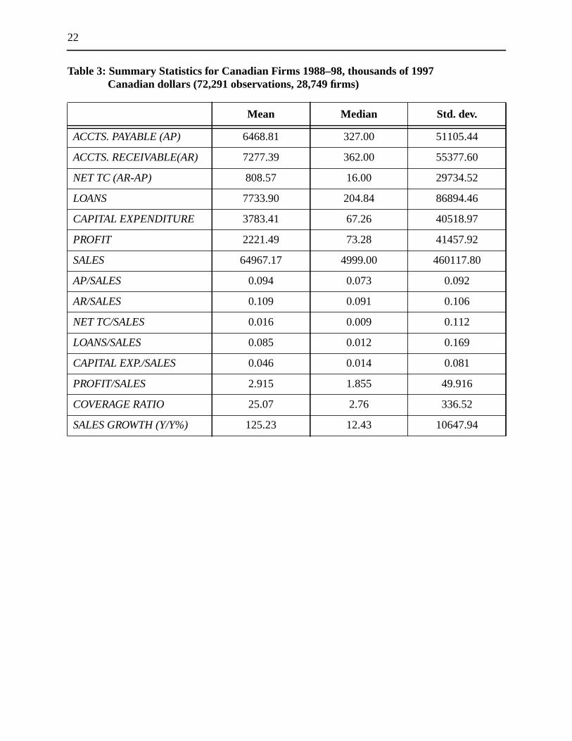
Table 3 provides summary statistics for the variables and observations used in the main regression
analyses. Perhaps the most striking feature of the data is that the mean and median values are very
different for most variables, often by a factor of 10 or more. This reflects the fact that the
population of Canadian firms consists of many small firms and a few large firms. The means are
strongly influenced by the large firms and are usually much higher than the median values. For
accounts payable, which measures the utilization of trade credit, the mean is $6.5 million but the
median is only $327 thousand in 1997 Canadian dollars. The mean accounts receivable are
somewhat larger than accounts payable at $7.3 million, but the median value is only
$362 thousand. Net trade balances are quite small, but similarly skewed. Consistent with the
reported importance of trade credit as a source of finance for small firms, accounts payable and
accounts receivable are comparable in size to the bank loan amounts for this sample of firms.
Capital expenditures and profits are considerably smaller, with mean values of $3.8 million and
$2.2 million, respectively. Sales average $65 million, with a median value of $5 million.
Scaling the variables by sales gives the proportion of trade credit used or supplied by the firm. The
ratios are less skewed, since the means and medians are fairly similar for most variables. The
means and medians forAP/SALESare 0.094 and 0.073, respectively, and forAR/SALESthe mean
and median values are 0.109 to 0.091. On balance, the net trade credit to sales is slightly positive
for these firms with non-negative sales growth. The Canadian data seem broadly consistent with
the findings of Petersen and Rajan (1997), who study U.S. trade credit data from 1987. In their
5. Statistics Canada.Financial and Taxation Statistics for Enterprises. Catalogue 61-219XPB, variousyears.
10
sample, the U.S. firms have meanAP/SALESof 0.044 for small firms and 0.116 for large firms,
and they find meanAR/SALES of 0.073 for small firms and 0.185 for large firms.
5. Estimation Method
Credit rationing is believed to primarily affect firms that have good investment projects, by
preventing them from fully borrowing against those opportunities. To operationalize this idea, I
assume that firms with good investment opportunities are those with non-negative sales growth
from the previous year, and my analysis focuses on those observations.
5.1 Estimation of trade credit usage
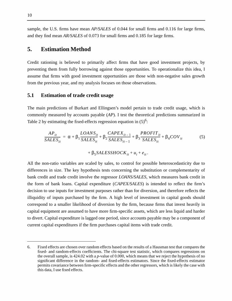
The main predictions of Burkart and Ellingsen’s model pertain to trade credit usage, which is
commonly measured by accounts payable (AP). I test the theoretical predictions summarized in
Table 2 by estimating the fixed-effects regression equation in (5)6:
(5)
.
All the non-ratio variables are scaled by sales, to control for possible heteroscedasticity due to
differences in size. The key hypothesis tests concerning the substitution or complementarity of
bank credit and trade credit involve the regressorLOANS/SALES, which measures bank credit in
the form of bank loans. Capital expenditure (CAPEX/SALES) is intended to reflect the firm’s
decision to use inputs for investment purposes rather than for diversion, and therefore reflects the
illiquidity of inputs purchased by the firm. A high level of investment in capital goods should
correspond to a smaller likelihood of diversion by the firm, because firms that invest heavily in
capital equipment are assumed to have more firm-specific assets, which are less liquid and harder
to divert. Capital expenditure is lagged one period, since accounts payable may be a component of
current capital expenditures if the firm purchases capital items with trade credit.
6. Fixed effects are chosen over random effects based on the results of a Hausman test that compares thefixed- and random-effects coefficients. The chi-square test statistic, which compares regressions onthe overall sample, is 424.02 with ap-value of 0.000, which means that we reject the hypothesis of nosignificant difference in the random- and fixed-effects estimators. Since the fixed-effects estimatorpermits covariance between firm-specific effects and the other regressors, which is likely the case withthis data, I use fixed effects.
APit
SALESit--------------------- α β1
LOANSit
SALESit----------------------- β2
CAPEXit 1–
SALESit 1–------------------------------ β3
PROFITit
SALESit-------------------------- β4COVit+ + + +=
β5SALESSHOCKit ui eit+ + +
11
Wealth is operationalized by net income before tax, referred to in this paper asPROFIT.7 The
interest coverage ratio (COV) is a standard measure of credit quality and is included in the
regression as a proxy for creditor security. A higher coverage ratio improves the likelihood of
repayment and reduces creditor vulnerability.
TheSALESSHOCKvariable controls for unexpected changes in demand conditions faced by the
firm, corresponding to changes in output prices (p) in the theoretical model. TheSALESSHOCK
variable consists of the residuals from an auxiliary ordinary least-squares (OLS) regression of
sales on a full set of industry and year dummy variables. The predictions from the auxiliary
regression produce the expected sales for a firm in a given year and industry, and the residuals
capture demand shocks faced by individual firms. I do not have a measure of trade credit financing
cost in the regression; however, Ng, Smith, and Smith (1999) and others observe that there is very
little variation in trade credit terms over time, but considerable cross-industry variation. I include
time and industry dummy variables in the regressions to control for these effects.
The predicted effects of the explanatory variables differ across firm groups, as shown by the signs
in Table 2. For the low-wealth firms, I expect that all the variables will have positive coefficients,
because an increase in any of them raises both credit limits, and, since these firms are at their
limits, their trade credit usage should increase. For the medium-wealth firms, the explanatory
variables will usually have negative coefficients, because they increase both credit limits, causing
these firms to substitute away from trade credit. There are some opposing effects for the medium-
wealth firms, soCAPEX/SALEShas a zero coefficient, andSALESSHOCKis ambiguous. All
coefficients are predicted to be zero for the high-wealth firms, because trade credit usage is
unrelated to financing decisions in Burkart and Ellingsen’s model.8
An important econometrics issue is that some of the regressors in equation (5) are likely to be
endogenous. In particular, bank credit is not likely to be exogenously determined, since a firm’s
decision regarding the use of bank credit may depend on its decision to use trade credit. Similarly,
it is not clear thatPROFITor COVare not determined within the model, in that firms with better
access to trade credit may have higher profits or higher coverage ratios. Unfortunately, finding
appropriate instruments from the available dataset of financial variables is difficult, because most
of the alternatives are not exogenous. The endogeneity problem potentially confounds
interpretation of the results: they should not be interpreted as describing a causal relationship.
7. Net income is broader than profits, but I use the terms interchangeably in this paper. The appendixprovides detailed variable definitions and data descriptions.
8. Other models show firms may use trade credit for non-financial reasons, such as reducing transactionscosts, as in Ferris (1981).
12
Nevertheless, I think the findings are informative about the relevant relationships and patterns of
trade credit behaviour across firm types.9
5.2 Estimation of trade credit supplied and net trade credit
To analyze trade credit supply behaviour, the dependent variable in the regression isAR/SALES.
The theoretical model predicts that a firm that is constrained in its bank credit will offer trade
credit as long as the trade credit extended earns as high a return as the firm’s investment project. I
expect that firms with slow sales growth probably have fewer good investment opportunities than
faster-growing firms, so I add an explanatory variable,GROWTH, to the regression equation for
trade credit supplied. TheGROWTHvariable is expected to have a negative coefficient. SinceAR
claims can be used as collateral to obtain additional bank loans, I expect a positive relationship
between trade credit supplied andLOANS/SALES, although it is not clear which way the causality
will run. The other variables should have the same signs as predicted above, because the firm still
faces a diversion decision—whether to divert bank credit or use it to finance accounts receivable
(trade credit lending).
Although the model does not deal explicitly with net trade credit (AR-AP), several other studies
examine the relationship between trade credit supplied and trade credit used. One can interpret
Burkart and Ellingsen’s main theoretical results concerning the effects that substitution or
complementarity between bank and trade credit have on net trade credit positions by considering
the effects of a reduction in the bank credit limit. Medium-wealth firms can increase their use of
trade credit to make up for the decrease in bank credit. They may also choose to decrease the
credit they supply,AR; or, perhaps to preserve good relationships with their customers, they may
keepAR the same. WhetherAR remains fixed or is decreased, net trade credit (AR-AP) will
decrease as long asAP increases by more thanARdecreases. Therefore, for medium-wealth firms,
I expect to see a positive coefficient on the bank loans variable in the regression results for net
trade credit.
For low-wealth firms, bank credit reductions decrease trade credit usageAP and may also lead
them to reduceAR. A reduction in bank credit increases net trade credit (AR-AP) for low-wealth
firms if ARremains constant or is reduced by less thanAP. If ARandAP are reduced by the same
amount in response to lower bank credit, then net trade credit is unchanged. Therefore, I expect
9. Standard approaches to the endogeneity problem, such as using lags as instruments and generalizedmethod of moment estimation methods, could be employed, but would result in the loss of a largenumber of observations on the small firms, because these firms usually have only one or two years ofdata. Future work will attempt to address the endogeneity issue by using simultaneous equations.
13
that the net trade credit for low-wealth firms is more negatively related or unrelated to the bank
credit variable.
5.3 Sample splitting and estimating wealth category thresholds
Because the theory predicts different behaviour for different wealth categories, the basic model in
equation (5) is estimated for each wealth group by adding dummy variables for low- and medium-
wealth categories and interacting those dummy variables with the other explanatory variables.
To define the high-, medium-, and low-wealth categories, one needs to find a lower and upper
threshold that distinguishes low wealth from medium wealth and medium wealth from high
wealth. Previous studies on credit rationing often use arbitrarily assigned thresholds, such as the
median or other quartiles. Since my sample has so many small firms and appears to be quite
skewed with respect to profits and other variables, there is likely to be a large proportion of credit-
constrained, low-wealth firms. Nevertheless, it is not obvious where the boundaries between
wealth groups are. Therefore, it seems appropriate to try to find the wealth thresholds using an
endogenous method.
I follow the approach recommended by Hansen (2000) to find endogenous thresholds. First, to
find the low-wealth threshold, I define aLOWdummy variable that equals one ifPROFITis below
a given value, which is allowed to range, in 1997 Canadian dollars, from -$50,000 to $174,000.
This range corresponds to between about the 10th and 75th percentiles of the profit variable,
giving a large window around the median, a natural starting point. TheLOW dummy and
interactions ofLOWwith the other five main regressors are added to the basic regression model,
which is then estimated separately for each value ofPROFITin the range. A comparison is made
of the sum of squared residuals from each regression, and the low-wealth threshold selected is the
value ofPROFIT that minimizes the sum of the squared residuals. This process yields a lower
profit threshold of $60,000, equal to about the 55th percentile ofPROFIT. Low-wealth firms are
therefore defined as those with profits of less than $60,000 in 1997 dollars.
The same process is used to find a second, upper threshold by defining aMEDIUM dummy
variable and interacting it with the other five regressors shown in equation (5). TheMEDIUM
dummy equals one whenPROFIT is greater than or equal to $60,000 and less than the upper
threshold value, which is allowed to range from $60,000 to $3.132 million, the 95th percentile.10
This second search process does not yield a distinct upper threshold, since the second value of
10. PROFITincreases by increments of $1,000 in the search for the lower threshold, and by increments of$5,000 in the search for the upper threshold.
14
profit that minimizes the sum of squared residuals is $61,000, not statistically different from the
other threshold. Therefore, this sample appears to have only one threshold, which implies that
there are no high-wealth, unconstrained firms, but that there are distinct categories of low-wealth
and medium-wealth firms. I test the robustness of this finding by imposing several different single
and double thresholds on the wealth categories.
6. Regression Results
6.1 Regression results for trade credit usage (AP/SALES)
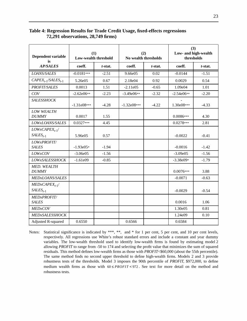
Table 4 shows the main regression estimates for accounts payable to sales. Model 1 reports the
results of estimating equation (5), including theLOWwealth dummy variable and the interactions
of LOWwith the other five regressors.LOWequals one ifPROFITis less than the estimated low-
wealth threshold of $60,000. Since the search process does not find a second threshold, I interpret
the data as having only low-wealth and medium-wealth firms, and the medium-wealth firms are
the reference group in model 1.
Overall, the estimates from model 1 conform quite well to the main predictions of Burkart and
Ellingsen’s model. The medium-wealth firms do seem to substitute trade credit for bank credit,
since the coefficient onLOANS/SALESis negative and significantly different from zero at the
1 per cent level. The low-wealth firms have a positive and significant coefficient onLOANS/
SALES, which implies that, for them, bank credit and trade credit are complements rather than
substitutes, consistent with the theory. All the other variables in model 1 have the predicted signs
for the medium-wealth firms, exceptPROFIT/SALES, for which the sign is contrary to the
predictions for both low- and medium-wealth firms. The contrary signs on thePROFIT/SALES
variable suggests that the theory’s cyclical implications do not match the data well; however,
neither coefficient is significantly different from zero at the 5 per cent level. The predictions for
variables other than bank loans hold up less well for the low-wealth firms. Three variables,
LOWxPROFIT/SALES, LOWxCOV,andLOWxSALESSHOCK, have signs contrary to predictions,
but they are also very small and not significant at the 5 per cent level.
Although the estimated relationships between bank credit and trade credit are statistically
significant, they do not appear to be economically significant. For the average medium-wealth
firm in the sample, an increase of one standard deviation in its ratio of bank credit to sales (from
0.085 to 0.245) results in a decrease in itsAP/SALESratio of just 0.003, reducing the firm’s
average ratio of trade credit usage from 0.094 to 0.091. For low-wealth firms, the estimated bank
loans coefficient of 0.0246 (-0.0181 + 0.0327) implies that a one-standard-deviation increase in
15
LOANS/SALESof 0.169 would result in an increase inAP/SALESof just 0.004, raising the firm’s
ratio to 0.098.
Model 1 relies on an estimated threshold to split the sample into low- and medium-wealth firms.
To test the robustness of this threshold, I also estimate the model using the 25th, 35th, 45th, 50th,
65th, 75th, 85th, and 95th percentiles ofPROFIT as the threshold to define theLOW dummy
variable. The results are qualitatively the same as reported for model 1 in Table 4. The coefficient
on LOWxLOANS/SALESis always positive and significant at the 1 or 5 per cent level for all the
thresholds tested. For medium-wealth firms, the coefficient on the bank loans variable is always
negative, and is significantly different from zero at the 5 per cent level when the low-wealth
threshold is anywhere from the 45th to 85th percentiles ofPROFIT, equal to a range, in 1997
Canadian dollars, of $25,000 to $443,000.
Model 2 in Table 4 shows regression results of estimating the model without any wealth
thresholds. This yields coefficient estimates that do not correspond very well to Burkart and
Ellingsen’s theoretical predictions for any of the three wealth categories.LOANS/SALEShas a
very small coefficient that is not statistically significant. This may reflect opposing signs for
different wealth groups that effectively cancel each other out when all the observations are pooled
together.
Even though the endogenous search method does not find a second threshold, the theory predicts
that there are two thresholds (three wealth categories). Therefore, in model 3, I also estimate a
version that arbitrarily imposes a second, upper threshold for wealth equal to the 90th percentile
of PROFIT, or $972,000. Model 3 has an additional dummy variable to indicate medium wealth,
equal to one when . The regression results for model 3 are such
that the bank credit variable,LOANS/SALES,is not significant for the high-wealth firms, but is
positive and significant for the low-wealth firms, as predicted by Burkart and Ellingsen. Model 3
also finds the predicted negative relationship between bank loans and trade credit usage for the
medium-wealth firms, but the estimated coefficient is not significant. Indeed, none of the
coefficient estimates for medium-wealth firms is statistically different from zero in model 3.
Thus, model 1 appears to be the most consistent with the theoretical predictions, and its key
findings hold under many different wealth thresholds and other robustness tests, as discussed in
section 6.3.
$60,000 PROFIT $972,000<≤
16
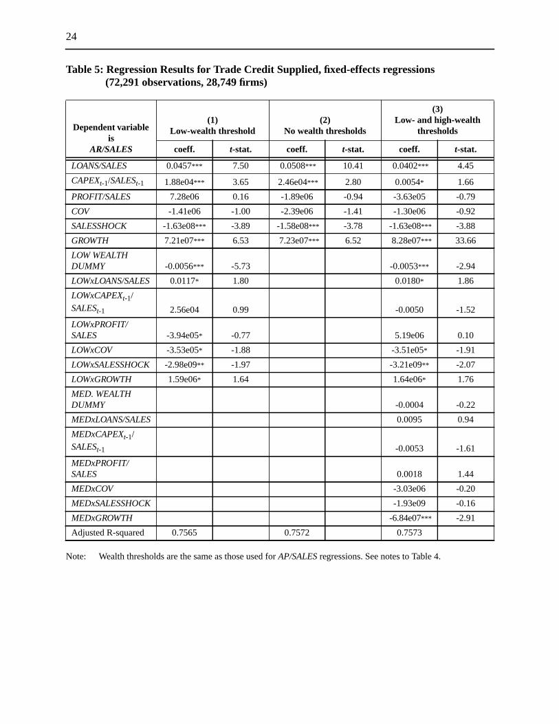
6.2 Regression results for trade credit supplied and net trade credit
Table 5 shows the regression results for trade credit supplied, and Table 6 shows the regression
results for net trade credit supplied.11 In all the regressions in Table 5, the dummy variable for low
wealth is negative and significant, which implies that those firms supply proportionally less trade
credit than wealthier firms, as one might expect. One of the main implications of Burkart and
Ellingsen’s model, with respect toAR/SALES, is that faster-growing firms provide less trade credit
than slower-growing firms. This hypothesis is quite clearly rejected by my data, since the
coefficient on sales growth has a positive sign in all the regressions, as do the interaction terms
LOWxGROWTHandMEDxGROWTH. The sample firms increase trade credit relative to sales as
sales growth increases, but the coefficients are very small and not economically significant.
I do find that increases in bank credit correspond to significant increases inAR/SALES. This
positive relationship is consistent with Burkart and Ellingsen’s argument that firms use trade
credit claims to obtain more bank credit, although that argument implies the causality goes from
AR/SALESto LOANS/SALES. Another possible interpretation is that, as firms obtain more bank
credit, they pass some of it on to their credit-rationed customers via trade credit, consistent with
most of the financing theories of trade credit and other empirical studies. Surprisingly, however,
LOWxLOANS/SALESis positive and significant at the 10 per cent level, which means that the low-
wealth firms provide proportionally more trade credit for a given increase in their bank credit than
other firms do. Since Petersen and Rajan (1997) find similar results, I explore this issue further in
the robustness tests described in section 6.3.
I argued earlier that the hypotheses of Burkart and Ellingsen’s model could be extended to
generate testable predictions for net trade credit. Specifically, the bank credit variable is expected
to have a positive influence on the ratio of net trade credit to sales for medium-wealth firms, and to
have a negative or zero coefficient for low-wealth firms. The regression results in Table 6 provide
considerable support for this prediction, since the coefficient onLOANS/SALESis positive and
highly significant, consistent with the prediction for medium-wealth firms. Also in model 1, the
coefficient forLOWxLOANS/SALESis negative and significant, so there is a significant difference
from the other firms. This difference implies that medium-wealth firms increase net trade credit
more for a given increase in bank credit than low-wealth firms do. Nevertheless, the estimated
coefficient for bank loans for the low-wealth firms is 0.0430, contrary to the prediction of a
negative or zero coefficient. The regression results for trade credit supplied and net trade credit
11. The regression results reported in Tables 5 and 6 are based on the same wealth thresholds as those inTable 4.
17
provide some support for the hypotheses of Burkart and Ellingsen’s model, especially with
respect to medium-wealth firms.
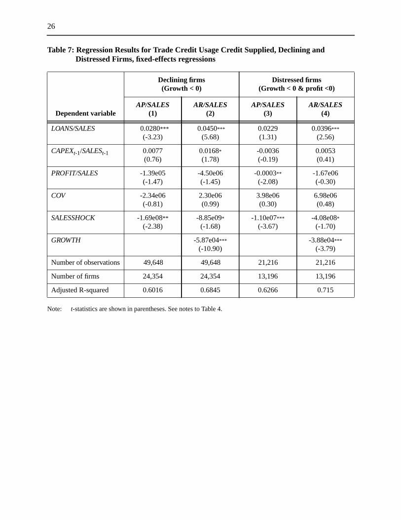
6.3 Robustness tests
Although there are no explicit predictions about the trade credit behaviour of firms that may be
financially distressed in Burkart and Ellingsen’s model, Petersen and Rajan (1997) find that
distressed firms offer proportionally more trade credit than other firms. I find something similar
for growing firms with low wealth in Table 5. To compare my findings more directly with those of
Petersen and Rajan, I also estimate the basic model (no wealth thresholds) for firms with negative
sales growth, and for distressed firms. Distressed firms are defined as those with negative sales
growth and negative profit. The results are reported in Table 7. In columns 1 and 3, trade credit
usage increases as bank credit increases for both the declining and distressed firms. This is not
surprising, since declining and distressed firms are likely to be constrained in their access to both
bank and trade credit, leading to a complementary relationship between the two types of credit, as
in the earlier findings for low-wealth firms.
With respect to trade credit supplied, theAR/SALESregressions indicate that both declining and
distressed firms increase their trade credit supplied when their bank loans increase. This finding is
consistent with that of Petersen and Rajan, but is surprising, especially for the distressed firms.
Firms that are in trouble might decrease the trade credit they provide if bank credit declines, but
one would not expect them to increase their supply of trade credit if their access to bank credit
improves. Wilner (2000) provides a potential explanation. Customers of distressed suppliers may
have high market power, such that dependent trade creditors are required by their large customers
to provide credit even in periods of financial distress. A financially distressed supplier may be
distressed because its largest customers are distressed. Wilner predicts that large, financially
distressed customers prefer trade credit from a dependent supplier to credit from sources that are
less dependent on them for future profits. My sample data may be picking up on this kind of
exploitation of market power.
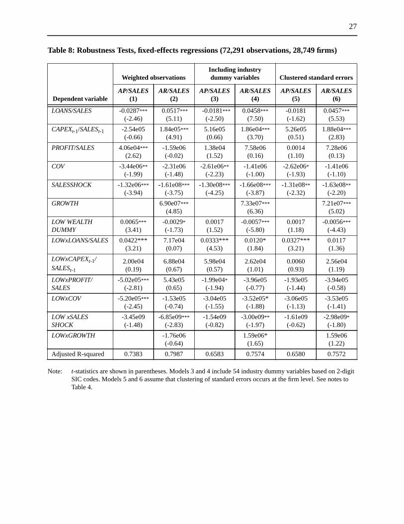
To further test the robustness of my main findings, I also analyze several modified versions of
regression model 1 in Tables 4 and 5. Table 8 reports the results of estimating the main regressions
for trade credit usage and trade credit supplied with weighted observations, dummy variables for
industry, and controls for clustered standard errors. Weighted data can help adjust for the stratified
sampling methods used to collect some of the data. Industry-specific trade credit terms and other
industry-specific factors may be better controlled for with the addition of industry dummy
variables. Finally, if the data are independent across firms but not necessarily independent over
18
time within firms, controlling for clustering in the data may be appropriate. This correction
increases the standard errors in the coefficient estimates and therefore reduces thet-statistics.
The results of these robustness tests are generally quite similar to the findings for model 1
reported in Tables 4 and 5. Regressions with weighted observations have somewhat larger
coefficients for the bank credit variables in theAP/SALESregressions. Adding industry dummy
variables makes almost no difference to any of the coefficients. Correcting for clustered standard
errors reduces the precision of the coefficient estimates and weakens the findings somewhat.
Specifically,LOANS/SALESin column 5 of Table 8 is no longer statistically significant, although
the coefficient onLOWxLOANS/SALES remains significant.
7. Conclusions
Burkart and Ellingsen (2004) model trade credit as a means to help overcome a potential moral
hazard problem of borrowers diverting resources for private gain. This problem causes credit
rationing of both bank credit and trade credit, but because inputs are harder to divert than cash and
suppliers have a monitoring advantage for input use, suppliers can provide credit when banks
cannot. Burkart and Ellingsen’s model explains why firms of different wealth categories face
different degrees of credit rationing and have different patterns of trade credit usage. Aggregate
investment is higher when trade credit is available because it allows medium- and low-wealth
firms to invest more than their bank credit constraint would permit.
My findings on trade credit usage provide fairly strong support for the theory’s main predictions,
particularly with respect to medium-wealth firms. For those firms, bank credit and trade credit
usage are negatively related, consistent with trade credit playing the role of a less-desirable form
of credit when bank credit is exhausted. Medium-wealth firms can increase their reliance on trade
credit if bank credit becomes less available. The firms identified as low-wealth have a positive,
complementary relationship between their bank credit and trade credit use, which suggests that
they are constrained in both trade credit and bank credit markets. The findings on trade credit
usage seem robust to a large range of possible wealth thresholds. Nevertheless, the estimated
effects for the low- and medium-wealth firms appear to be economically small despite their strong
statistical significance.
These findings also suggest that there are very few high-wealth, unconstrained firms in Canada.
This is consistent with Nilsen (2002), who finds that all but the largest, bond-rated firms appear to
be finance-constrained. The data do not seem to support the view that firms supply less trade
credit when their investment opportunities increase, insofar as sales growth captures investment

19
opportunities. I find that faster sales growth corresponds to a provision of more trade credit.
Consistent with Petersen and Rajan (1997), I also find that low-wealth, declining, and distressed
firms provide proportionally more trade credit than more wealthy firms do. Further research
should use better proxies for creditor vulnerability and trade credit interest rates than are available
for this study. Further empirical work to discover why distressed firms supply more trade credit
than other firms, and the cyclical implications of this behaviour, would also be of interest.
20
References
Biais, B. and C. Gollier. 1997. “Trade Credit and Credit Rationing.”Review of FinancialStudies10(4): 903–37.
Bitros, G.C. 1979. “Neoclassical Theory of Trade Credit: A Critique and a Reformulation.”Econometrica 47(1): 199–202.
Burkart, M. and T. Ellingsen. 2004. “In-Kind Finance: A Theory of Trade Credit.”AmericanEconomic Review 94(3): 569–90.
Demirgüç-Kunt, A. and V. Maksimovic. 2001. “Firms as Financial Intermediaries: Evidence fromTrade Credit Data.” World Bank Working Paper.
Dun and Bradstreet. 1970.Handbook of Credit Terms. New York: Dun and Bradstreet.
Emery, G.W. 1984. “A Pure Financial Explanation for Trade Credit.”Journal of Financial andQuantitative Analysis 19(3): 271–85.
Ferris, J.S. 1981. “A Transactions Cost Theory of Trade Credit Use.”Quarterly Journal ofEconomics 96(2): 243–70.
Hansen, B.E. 2000. “Sample Splitting and Threshold Estimation.”Econometrica 68(3): 575–603.
Hubbard, G. 1998. “Capital Market Imperfections and Investment.”Journal of EconomicLiterature 36(1): 193–225.
Jain, N. 2001. “Monitoring Costs and Trade Credit.”Quarterly Review of Economics andFinance41: 89–110.
Mian, S. and C.W. Smith. 1992. “Accounts Receivable Management Policy: Theory andEvidence.”Journal of Finance 47: 169–200.
Nadiri, M.I. 1969. “The Determinants of Trade Credit in the U.S. Total Manufacturing Sector.”Econometrica 47(1): 408–23.
Ng, C.K., J.K. Smith, and R. Smith. 1999. “Evidence on the Determinants of Credit Terms Usedin Interfirm Trade.”Journal of Finance 54(3): 1109–29.
Nilsen, J. 2002. “Trade Credit and the Bank Lending Channel.”Journal of Money, Credit andBanking 34(1): 227–53.
Petersen, M.A. and R.G. Rajan. 1997. “Trade Credit: Theories and Evidence.”Review ofFinancial Studies 10(3): 661–91.
Schwartz, R.A. 1974. “An Economic Model of Trade Credit.”Journal of Financial andQuantitative Analysis 9: 643–57.
Statistics Canada. 1998.Financial and Taxation Statistics for Enterprises. Catalogue 61-219XPB.
Wilner, B. 2000. “The Exploitation of Relationships in Financial Distress: The Case of TradeCredit.” Journal of Finance 55(1): 153–78.

21
Table 1: Borrowing and Investment Behaviour by Entrepreneurs in Various WealthCategories in Burkart and Ellingsen’s Model
Table 2: Sign Predictions for Trade Credit Usage in Burkart and Ellingsen’s Model
High-wealth Medium-wealth Low-wealth
Bank credit usage
Trade credit usage
Investment level
Model parameterRegression
proxyPredicted change in trade credit use from an
increase in explanatory variable
Low-wealthMedium-
wealth High-wealth
Bank credit(BC) LOANS/SALES + - 0
Input illiquidity CAPEX/SALES + 0 0
Wealth PROFIT/SALES + - 0
Creditor security COVRATIO + - 0
Product price(p) SALESSHOCK + ? 0
Trade credit cost n.a. - ? 0
BC BC< BC BC= BC BC=
TC 0= TC TC< TC TC=
I I *( r BC)= I I *( rTC)= I I *( rTC)<
-β( )
ω( )
-ϕ( )
rTC( )
22
Table 3: Summary Statistics for Canadian Firms 1988–98, thousands of 1997Canadian dollars (72,291 observations, 28,749 firms)
Mean Median Std. dev.
ACCTS. PAYABLE (AP) 6468.81 327.00 51105.44
ACCTS. RECEIVABLE(AR) 7277.39 362.00 55377.60
NET TC (AR-AP) 808.57 16.00 29734.52
LOANS 7733.90 204.84 86894.46
CAPITAL EXPENDITURE 3783.41 67.26 40518.97
PROFIT 2221.49 73.28 41457.92
SALES 64967.17 4999.00 460117.80
AP/SALES 0.094 0.073 0.092
AR/SALES 0.109 0.091 0.106
NET TC/SALES 0.016 0.009 0.112
LOANS/SALES 0.085 0.012 0.169
CAPITAL EXP./SALES 0.046 0.014 0.081
PROFIT/SALES 2.915 1.855 49.916
COVERAGE RATIO 25.07 2.76 336.52
SALES GROWTH (Y/Y%) 125.23 12.43 10647.94
23
Table 4: Regression Results for Trade Credit Usage, fixed-effects regressions72,291 observations, 28,749 firms)
Notes: Statistical significance is indicated by ***, **, and * for 1 per cent, 5 per cent, and 10 per cent levels,respectively. All regressions use White’s robust standard errors and include a constant and year dummyvariables. The low-wealth threshold used to identify low-wealth firms is found by estimating model 2allowing PROFITto range from -50 to 174 and selecting the profit value that minimizes the sum of squaredresiduals. This method defines low-wealth firms as those withPROFIT<$60,000 (about the 55th percentile).The same method finds no second upper threshold to define high-wealth firms. Models 2 and 3 providerobustness tests of the thresholds. Model 3 imposes the 90th percentile ofPROFIT, $972,000, to definemedium wealth firms as those with . See text for more detail on the method androbustness tests.
Dependent variableis
AP/SALES
(1)Low-wealth threshold
(2)No wealth thresholds
(3)Low- and high-wealth
thresholds
coeff. t-stat. coeff. t-stat. coeff. t-stat.
LOANS/SALES -0.0181*** -2.51 9.66e05 0.02 -0.0144 -1.51
CAPEXt-1/SALESt-1 5.26e05 0.67 2.18e04 0.92 0.0029 0.54
PROFIT/SALES 0.0013 1.51 -2.11e05 -0.65 1.09e04 1.01
COV -2.62e06** -2.23 -3.49e06** -2.32 -2.54e06** -2.20
SALESSHOCK-1.31e08*** -4.28 -1.32e08*** -4.22
-1.30e08*** -4.33
LOW WEALTHDUMMY 0.0017 1.55 0.0086*** 4.30
LOWxLOANS/SALES 0.0327*** 4.45 0.0278*** 2.81
LOWxCAPEXt-1/SALESt-1 5.96e05 0.57 -0.0022 -0.41
LOWxPROFIT/SALES -1.93e05* -1.94 -0.0016 -1.42
LOWxCOV -3.06e05 -1.56 -3.09e05 -1.56
LOWxSALESSHOCK -1.61e09 -0.85 -3.38e09* -1.79
MED. WEALTHDUMMY 0.0076*** 3.88
MEDxLOANS/SALES -0.0071 -0.63
MEDxCAPEXt-1/SALESt-1 -0.0029 -0.54
MEDxPROFIT/SALES 0.0016 1.06
MEDxCOV 1.30e05 0.81
MEDxSALESSHOCK 1.24e09 0.10
Adjusted R-squared 0.6550 0.6566 0.6584
60 PROFIT 972<≤
24
Table 5: Regression Results for Trade Credit Supplied, fixed-effects regressions(72,291 observations, 28,749 firms)
Note: Wealth thresholds are the same as those used forAP/SALES regressions. See notes to Table 4.
Dependent variableis
AR/SALES
(1)Low-wealth threshold
(2)No wealth thresholds
(3)Low- and high-wealth
thresholds
coeff. t-stat. coeff. t-stat. coeff. t-stat.
LOANS/SALES 0.0457*** 7.50 0.0508*** 10.41 0.0402*** 4.45
CAPEXt-1/SALESt-1 1.88e04*** 3.65 2.46e04*** 2.80 0.0054* 1.66
PROFIT/SALES 7.28e06 0.16 -1.89e06 -0.94 -3.63e05 -0.79
COV -1.41e06 -1.00 -2.39e06 -1.41 -1.30e06 -0.92
SALESSHOCK -1.63e08*** -3.89 -1.58e08*** -3.78 -1.63e08*** -3.88
GROWTH 7.21e07*** 6.53 7.23e07*** 6.52 8.28e07*** 33.66
LOW WEALTHDUMMY -0.0056*** -5.73 -0.0053*** -2.94
LOWxLOANS/SALES 0.0117* 1.80 0.0180* 1.86
LOWxCAPEXt-1/SALESt-1 2.56e04 0.99 -0.0050 -1.52
LOWxPROFIT/SALES -3.94e05* -0.77 5.19e06 0.10
LOWxCOV -3.53e05* -1.88 -3.51e05* -1.91
LOWxSALESSHOCK -2.98e09** -1.97 -3.21e09** -2.07
LOWxGROWTH 1.59e06* 1.64 1.64e06* 1.76
MED. WEALTHDUMMY -0.0004 -0.22
MEDxLOANS/SALES 0.0095 0.94
MEDxCAPEXt-1/SALESt-1 -0.0053 -1.61
MEDxPROFIT/SALES 0.0018 1.44
MEDxCOV -3.03e06 -0.20
MEDxSALESSHOCK -1.93e09 -0.16
MEDxGROWTH -6.84e07*** -2.91
Adjusted R-squared 0.7565 0.7572 0.7573

25
Table 6: Regression Results for Net Trade Credit Supplied, fixed-effects regressions(72,291 observations, 28,749 firms)
Note: Wealth thresholds are the same as those forAP/SALES regressions. See notes to Table 4.
Dependent variableis
(AR-AP)/SALES
(1)Low-wealth threshold
(2)No wealth thresholds
(3)Low- and high-wealth
thresholds
coeff. t-stat. coeff. t-stat. coeff. t-stat.
LOANS/SALES 0.0639*** 8.02 0.0508*** 7.84 0.0546*** 5.05
CAPEXt-1/SALESt-1 1.36e04*** 3.01 3.07e05 0.14 0.0026 0.51
PROFIT/SALES -1.29e04 -1.60 3.63e06 0.09 -1.45e04* -1.64
COV 1.21e06 1.11 1.10e06 1.01 1.25e06 1.15
SALESSHOCK -3.29e09 -1.44 -2.62e09 -1.23 -3.32e09 -1.45
GROWTH 9.66e08*** 2.81 1.04e07*** 3.03 9.40e08*** 3.60
LOW WEALTHDUMMY -0.0074*** -6.13 -0.0139*** -6.28
LOWxLOANS/SALES -0.0209*** -2.46 -0.0099 -0.84
LOWxCAPEXt-1/SALESt-1 -3.27e04 -0.27 -0.0028 -0.53
LOWxPROFIT/SALES 1.55e04* 1.68 1.69e04* 1.70
LOWxCOV -4.71e06 -0.45 -4.11e06 -0.39
LOWxSALESSHOCK -1.32e09 -0.88 2.35e10 0.16
LOWxGROWTH 2.74e07 0.35 4.25e07 0.56
MED. WEALTHDUMMY -0.0080*** -3.65
MEDxLOANS/SALES 0.0165 1.25
MEDxCAPEXt-1/SALESt-1 -0.0025 -0.48
MEDxPROFIT/SALES 1.08e05 0.05
MEDxCOV -1.60e05 -1.28
MEDxSALESSHOCK -3.19e09 -0.25
MEDxGROWTH 4.02e09 0.02
Adjusted R-squared 0.6881 0.6890 0.6892
26
Table 7: Regression Results for Trade Credit Usage Credit Supplied, Declining andDistressed Firms, fixed-effects regressions
Note: t-statistics are shown in parentheses. See notes to Table 4.
Dependent variable
Declining firms(Growth < 0)
Distressed firms(Growth < 0 & profit <0)
AP/SALES(1)
AR/SALES(2)
AP/SALES(3)
AR/SALES(4)
LOANS/SALES 0.0280***(-3.23)
0.0450***(5.68)
0.0229(1.31)
0.0396***(2.56)
CAPEXt-1/SALESt-1 0.0077(0.76)
0.0168*(1.78)
-0.0036(-0.19)
0.0053(0.41)
PROFIT/SALES -1.39e05(-1.47)
-4.50e06(-1.45)
-0.0003**(-2.08)
-1.67e06(-0.30)
COV -2.34e06(-0.81)
2.30e06(0.99)
3.98e06(0.30)
6.98e06(0.48)
SALESSHOCK -1.69e08**(-2.38)
-8.85e09*(-1.68)
-1.10e07***(-3.67)
-4.08e08*(-1.70)
GROWTH -5.87e04***(-10.90)
-3.88e04***(-3.79)
Number of observations 49,648 49,648 21,216 21,216
Number of firms 24,354 24,354 13,196 13,196
Adjusted R-squared 0.6016 0.6845 0.6266 0.715
27
Table 8: Robustness Tests, fixed-effects regressions (72,291 observations, 28,749 firms)
Note: t-statistics are shown in parentheses. Models 3 and 4 include 54 industry dummy variables based on 2-digitSIC codes. Models 5 and 6 assume that clustering of standard errors occurs at the firm level. See notes toTable 4.
Dependent variable
Weighted observationsIncluding industrydummy variables Clustered standard errors
AP/SALES(1)
AR/SALES(2)
AP/SALES(3)
AR/SALES(4)
AP/SALES(5)
AR/SALES(6)
LOANS/SALES -0.0287***(-2.46)
0.0517***(5.11)
-0.0181***(-2.50)
0.0458***(7.50)
-0.0181(-1.62)
0.0457***(5.53)
CAPEXt-1/SALESt-1 -2.54e05(-0.66)
1.84e05***(4.91)
5.16e05(0.66)
1.86e04***(3.70)
5.26e05(0.51)
1.88e04***(2.83)
PROFIT/SALES 4.06e04***(2.62)
-1.59e06(-0.02)
1.38e04(1.52)
7.58e06(0.16)
0.0014(1.10)
7.28e06(0.13)
COV -3.44e06**(-1.99)
-2.31e06(-1.48)
-2.61e06**(-2.23)
-1.41e06(-1.00)
-2.62e06*(-1.93)
-1.41e06(-1.10)
SALESSHOCK -1.32e06***(-3.94)
-1.61e08***(-3.75)
-1.30e08***(-4.25)
-1.66e08***(-3.87)
-1.31e08**(-2.32)
-1.63e08**(-2.20)
GROWTH 6.90e07***(4.85)
7.33e07***(6.36)
7.21e07***(5.02)
LOW WEALTHDUMMY
0.0065***(3.41)
-0.0029*(-1.73)
0.0017(1.52)
-0.0057***(-5.80)
0.0017(1.18)
-0.0056***(-4.43)
LOWxLOANS/SALES 0.0422***(3.21)
7.17e04(0.07)
0.0333***(4.53)
0.0120*(1.84)
0.0327***(3.21)
0.0117(1.36)
LOWxCAPEXt-1/
SALESt-12.00e04(0.19)
6.88e04(0.67)
5.98e04(0.57)
2.62e04(1.01)
0.0060(0.93)
2.56e04(1.19)
LOWxPROFIT/SALES
-5.02e05***(-2.81)
5.43e05(0.65)
-1.99e04*(-1.94)
-3.96e05(-0.77)
-1.93e05(-1.44)
-3.94e05(-0.58)
LOWxCOV -5.20e05***(-2.45)
-1.53e05(-0.74)
-3.04e05(-1.55)
-3.52e05*(-1.88)
-3.06e05(-1.13)
-3.53e05(-1.41)
LOW xSALESSHOCK
-3.45e09(-1.48)
-6.85e09***(-2.83)
-1.54e09(-0.82)
-3.00e09**(-1.97)
-1.61e09(-0.62)
-2.98e09*(-1.80)
LOWxGROWTH -1.76e06(-0.64)
1.59e06*(1.65)
1.59e06(1.22)
Adjusted R-squared 0.7383 0.7987 0.6583 0.7574 0.6580 0.7572
28
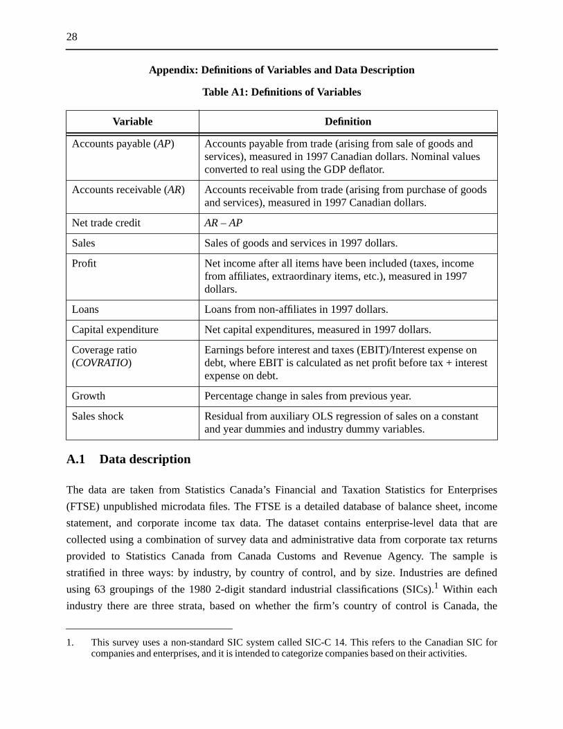
Appendix: Definitions of Variables and Data Description
Table A1: Definitions of Variables
A.1 Data description
The data are taken from Statistics Canada’s Financial and Taxation Statistics for Enterprises
(FTSE) unpublished microdata files. The FTSE is a detailed database of balance sheet, income
statement, and corporate income tax data. The dataset contains enterprise-level data that are
collected using a combination of survey data and administrative data from corporate tax returns
provided to Statistics Canada from Canada Customs and Revenue Agency. The sample is
stratified in three ways: by industry, by country of control, and by size. Industries are defined
using 63 groupings of the 1980 2-digit standard industrial classifications (SICs).1 Within each
industry there are three strata, based on whether the firm’s country of control is Canada, the
Variable Definition
Accounts payable (AP) Accounts payable from trade (arising from sale of goods andservices), measured in 1997 Canadian dollars. Nominal valuesconverted to real using the GDP deflator.
Accounts receivable (AR) Accounts receivable from trade (arising from purchase of goodsand services), measured in 1997 Canadian dollars.
Net trade credit AR – AP
Sales Sales of goods and services in 1997 dollars.
Profit Net income after all items have been included (taxes, incomefrom affiliates, extraordinary items, etc.), measured in 1997dollars.
Loans Loans from non-affiliates in 1997 dollars.
Capital expenditure Net capital expenditures, measured in 1997 dollars.
Coverage ratio(COVRATIO)
Earnings before interest and taxes (EBIT)/Interest expense ondebt, where EBIT is calculated as net profit before tax + interestexpense on debt.
Growth Percentage change in sales from previous year.
Sales shock Residual from auxiliary OLS regression of sales on a constantand year dummies and industry dummy variables.
1. This survey uses a non-standard SIC system called SIC-C 14. This refers to the Canadian SIC forcompanies and enterprises, and it is intended to categorize companies based on their activities.
29
United States, or another country. Finally, within the country-of-control stratum, there are
multiple size categories based on the firm’s assets or revenues. The largest firms in each industry
are sampled with certainty, although the size bounds vary by industry. For most industries, this
“take-all” stratum consists of the largest firms, which have assets or annual revenues of more than
$25 million in current dollars. The second, “take-some” stratum consists of smaller firms that are
randomly selected for inclusion in the survey. In the take-some stratum, data are collected through
a mix of surveys and administrative tax files. The final stratum of the sample consists of the
smallest firms, which were not surveyed, so all their data come from tax return files.
I select only the non-financial firms from the dataset, and also remove observations from the
sample if regression variables seem to have very extreme values. Specifically, I restrict the sample
to those observations where the dependent variables in the regressions, the ratios of accounts
payable to sales and accounts receivable to sales, are between zero and one; this removes
approximately 1 per cent of the original observations. Observations where sales are negative are
also omitted, as are the cases where ratios of capital expenditures to sales or bank loans to sales
are zero or greater than the 95th percentile value.
Bank of Canada Working PapersDocuments de travail de la Banque du Canada
Working papers are generally published in the language of the author, with an abstract in both officiallanguages.Les documents de travail sont publiés généralement dans la langue utilisée par les auteurs; ils sontcependant précédés d’un résumé bilingue.
Copies and a complete list of working papers are available from:Pour obtenir des exemplaires et une liste complète des documents de travail, prière de s’adresser à:
Publications Distribution, Bank of Canada Diffusion des publications, Banque du Canada234 Wellington Street, Ottawa, Ontario K1A 0G9 234, rue Wellington, Ottawa (Ontario) K1A 0G9E-mail: [email protected] Adresse électronique : [email protected] site: http://www.bankofcanada.ca Site Web : http://www.banqueducanada.ca
20042004-48 An Empirical Analysis of the Canadian Term
Structure of Zero-Coupon Interest Rates D.J. Bolder, G. Johnson, and A. Metzler
2004-47 The Monetary Origins of Asymmetric Informationin International Equity Markets G.H. Bauer and C. Vega
2004-46 Une approche éclectique d’estimation du PIBpotentiel pour le Royaume-Uni C. St-Arnaud
2004-45 Modelling the Evolution of Credit Spreadsin the United States S.M. Turnbull and J. Yang
2004-44 The Transmission of World Shocks toEmerging-Market Countries: An Empirical Analysis B. Desroches
2004-43 Real Return Bonds, Inflation Expectations,and the Break-Even Inflation Rate I. Christensen, F. Dion, and C. Reid
2004-42 International Equity Flows and Returns: AQuantitative Equilibrium Approach R. Albuquerque, G. Bauer, and M. Schneider
2004-41 Characterization of the Dynamic Effects of FiscalShocks in a Small Open Economy N. Rebei
2004-40 Prévision et analyse de la production manufacturièreau Canada : comparaison de modèles linéaires etnon linéaires F. Demers
2004-39 A Forecasting Model for Inventory Investmentsin Canada M. Chacra and M. Kichian
2004-38 Finance Constraints and Inventory Investment:Empirical Tests with Panel Data R. Cunningham
2004-37 The Implications of Transmission and InformationLags for the Stabilization Bias and Optimal Delegation J.-P. Lam and F. Pelgrin
2004-36 Optimal Taylor Rules in an Estimated Model ofa Small Open Economy S. Ambler, A. Dib, and N. Rebei
2004-35 The U.S. New Keynesian Phillips Curve: AnEmpirical Assessment A. Guay and F. Pelgrin