1

Do Companies Benefit from Public Research Organizations?

The Impact of Fraunhofer

Diego Comin,a Georg Licht,

b Maikel Pellens,

b and Torben Schubert

c

a Dartmouth College, Hanover (United States)

b Centre for European Economic Research (ZEW), Mannheim (Germany)

c Lund University, Lund (Sweden)

Executive summary

Since its inception in 1949, the Fraunhofer-Gesellschaft (FhG) has become Europe’s largest applied

research organization. Today, it has more than 60 research institutes in Germany covering a wide

range of topics in the natural sciences, engineering, informatics, and economics/social sciences. Taken

together, Fraunhofer has approximately 24,500 employees and commands an annual budget of over

€2.1 billion. Not only is Fraunhofer successful as a private organization, but it is also recognized for

providing the economy with unique scientific knowledge crucial for the development of new and

innovative goods and services. Founded with the dedicated mission to bridge the gap between basic

science, technological development and commercial application, Fraunhofer has grown to be an

attractive partner for industry. About 35% of its budget is financed through projects commissioned by

industrial clients.

While the lasting and continuous commitment of Germany industry to Fraunhofer is indicative of its

relevance for commercial innovation processes, the actual impact Fraunhofer has in terms of company

performance has not been subjected to rigorous empirical testing. Available knowledge on the

importance of Fraunhofer so far often relies on anecdotal evidence of particularly visible successes,

such as the development of MP3 technology. While reference to specific successes can be insightful, a

broad and solid empirical account of Fraunhofer’s effects on the economy is needed for at least two

reasons. First, being able to demonstrate the positive effect of Fraunhofer on the economy helps make

the case for the allocation of public funds to research institutions such as Fraunhofer. Second, and

arguably even more important, knowledge about the effects and in specific the conditions under which

they emerge can help to improve and tailor the ways in which Fraunhofer organizes itself. Thus,

knowledge on the specific contexts in which Fraunhofer’s inputs are particularly valuable can give

insights into specific paths to improve the Fraunhofer model.

This study tries to develop a deeper understanding of Fraunhofer’s contribution to society by

estimating the causal effects of engaging in contract research with Fraunhofer on company

performance. To study this question, we combined the Mannheim Innovation Panel, which has

information on the performance and innovation activity of a large number of German companies, with

a confidential dataset containing information on all the research contracts signed by Fraunhofer with

German companies during the 1997-2014 period. Analyzing a wide range of effects while controlling

2

for econometric issues such as selection, unobserved heterogeneity, and simultaneity, our core results

demonstrate significant and sizeable causal effects of research contracts with Fraunhofer on company

performance. Specifically, we show that Fraunhofer contracts offer considerable growth potential for

companies. In the year after a Fraunhofer interaction, companies experience a 9% increase in sales and

a 7% increase in employment. Those increases are accompanied by a shift in the employment

structure, as a Fraunhofer interaction also leads to a 1% increase in the share of employees with

tertiary education. In addition, the sales structure also shifts towards innovative products. We observe

that on average, a Fraunhofer interaction increases the share of companies’ sales of innovative

products by 1%.

Thus, we provide evidence that interactions with Fraunhofer do more than increase companies’ growth

rates; they also lead companies towards a more knowledge-intensive innovation path by expanding the

share of highly qualified personnel on the input side and increasing the weight of innovative products

in the sales base on the output side. Our results indicate that these effects are fairly persistent over

time, with some effects being documented even seven years after the interaction took place.

Furthermore, we can show that the effects are highly contingent on specific characteristics of the

companies and the interactions. In particular, the effects increase with the size of the project. The

effects are also larger for medium (50-249 employees) and large companies (250 or more employees)

than for small companies (up to 49 employees), and are more pronounced for companies in

manufacturing than in services. Finally, and especially worthy of note, companies experience much

higher impacts when they interact with Fraunhofer repeatedly. Given that our analysis already controls

for unobserved heterogeneity, the greater effects associated with repeated interactions suggest that the

value of Fraunhofer for companies is not generic, but specific to each individual relationship between

a Fraunhofer institute and a company. Thus, companies and the Fraunhofer institute must continuously

invest in long-lasting relationships if they are to leverage the full potential of interacting with

Fraunhofer. An important implication is that the broader economic value of Fraunhofer lies very much

at the micro-level of the specific relationships. These findings also provide an explanation for why

attempts to copy the Fraunhofer model, e.g. the Carnot institutes in France, usually have not lived up

to expectations: the value of Fraunhofer is rooted in its almost 70 years of experience, in which

repeated learning and continuous improvement of its business model have shaped its success today.

3

1 Introduction

Innovation is often touted as a direct path to productivity and output growth, business competitiveness,

and job creation. Yet in contrast to the social value of these potential outcomes, policies that favor

innovation are typically limited in scale and scope. Possible reasons for the failure to design effective

innovation policies include (i) lack of a deep understanding of the underpinnings of innovation

activity; (ii) insufficient guidance from economic theory, where most policies result in isomorphic

results and (iii) lack of empirical evidence on the effectiveness of various innovation policies.

In this study, we try to fill in these gaps by studying a unique research institution: the

Fraunhofer-Gesellschaft (FhG). Fraunhofer is a public research institution that was created in

Germany in 1949. Currently, Fraunhofer employs approximately 24,500 employees who conduct

applied research in all fields of science, leading to around 500 patents per year.1 In addition to their

basic research activity, Fraunhofer scientists also engage in contract research in which they solve

specific technological problems faced by individual companies. The fulfillment of the research

contracts often requires the use of the knowledge and technologies produced by Fraunhofer scientists.

The main goal of our investigation is to assess the impact of engaging in research contracts with FhG

for German companies. To study this question, we have combined two datasets. The first is the

Manheim Innovation Panel, which contains information on the performance and innovation activity of

a large number of companies in Germany. The second is a confidential dataset that contains

information on all the research contracts signed by Fraunhofer with German companies between 1997

and 2014.

The key challenge that a study such as ours needs to confront is the possibility that companies self-

select to contract with Fraunhofer. As a result, the sample of companies that engage in research

contracts is not random. Our analysis shows strong evidence that this is the case. In the presence of

selection bias, a positive correlation between engaging in contract research and the evolution of a

company’s performance may be driven by the fact that more productive companies are more likely to

engage in a contract, and does not necessarily mean that interacting with Fraunhofer had a positive

impact on the company.

We employ various empirical strategies to overcome the selection problem in estimating the effect of

engaging in contract research on the performance of German companies. These include (i) the use of

company fixed effects; (ii) re-weighting the non-treated companies to obtain a sample that is identical

to the treated companies in terms of observable variables (Azoulay et al., 2009); (iii) controlling for

pre-treatment trends; and (iv) using instruments that exploit the heteroscedasticity of the data (see

Lewbel, 2012). While issues of selection-induced heterogeneity remain, the robustness of the

1 See Comin (2015).

4

estimates when we perform them suggests that the estimated effects can be interpreted as the impact

on company performance caused by interacting with Fraunhofer.

Our key empirical findings are as follows:

1. One year after the fact, companies that interact with Fraunhofer tend to experience an increase

in sales on the order of 9%; in employment, 7%; share of innovative sales, approximately 1%;

average cost per employee, 1%; and share of workers with higher education, 1%. Of these, the

most robust are the effects on sales and employment.

2. The effects are not short-lived. We observe impacts even seven years after the interaction.

3. The benefits from interacting with Fraunhofer are not homogeneous among companies.

a. They are greater for companies that have interacted previously with Fraunhofer than

for those that interact for the first time.

b. They are greater when the projects have budgets of more than €100,000.

c. They are greater for manufacturing than for service companies.

d. They are greater for medium (50-249 employees) and large companies (250 or more

employees) than for small companies (up to 49 employees).

e. They are not affected by the age of the company and by the innovativeness of the

project.

The rest of the report is organized as follows: Section 2 introduces the datasets used in the analysis;

Section 3 presents the identification strategy; Section 4 presents the empirical results; and Section 5

concludes.

5

2 Data

The empirical analysis is based on two main data sources. The first is the project database provided by

the Fraunhofer-Gesellschaft (FhG), which covers all projects started between 1997 and 2014.2 For

each of the 131,158 projects, the database contains information on the Fraunhofer institute and

department involved; the client’s name and address; the title, short description and time span of the

project; and any project-related payments. Section 2.2 presents an in-depth description of the

information in the database.

The second data source is the Mannheim Innovation Panel (MIP), a survey conducted every year since

1993 by the Centre for European Economic Research on behalf of the German Federal Ministry for

Education and Research (BMBF). The MIP provides a representative annual sample of German

companies with five or more employees (see Aschhoff et al., 2013 for further details). It follows the

methodology outlined in the Oslo Manual (OECD and Eurostat, 2005) and is also Germany’s

contribution to the European Community Innovation Survey. The panel has been further amended with

data from Germany’s largest credit rating agency, Creditreform, for information on company’s age.

The present analysis makes use of the 2014 edition of the MIP, including information up to calendar

year 2013. Excluding companies that were observed fewer than three times, the MIP covers 198,385

observations of 30,125 companies between 1996 and 2014.3

Care was taken to guarantee the confidentiality of the agreements delivered by FhG, particularly with

regard to the identities of the client companies. The individuals responsible for matching the FhG data

and MIP data did not have access to the agreement data, but only to the name and address of the client

companies and organizations. Anonymous identifiers were constructed based on the matched data for

use in the remainder of the analysis. Furthermore, individuals involved in the database matching were

not involved in the remainder of the analysis.

Both datasets were merged by comparing company names and address information.4 Of the 131,158

projects in the Fraunhofer database, 46,651 projects could be linked to 7,781 distinct companies which

were surveyed at least once in the MIP. After eliminating companies for lack of response and the

condition that a company needed to be observed at least three times, the remaining 32,568 projects, or

24.8% of the projects in the database, were used in the final analysis. They represent 4,495 companies

in the MIP panel.

2 Approximately 10% of the projects in the database listed start dates before 1997. As these do not seem to

represent a full picture of the projects, we omit these from the further analysis. Any payments made to

Fraunhofer in the context of these projects in 1997 and onwards, however, are taken into account. 3 We retain information from 1996 to allow control variables to be lagged with one year.

4 The matching algorithm takes spelling deviations into account and assigns a score to each potential match.

Potential matches with some uncertainty were manually screened for accuracy.

6

There are several reasons for the large number of unmatched projects. First, 17% of projects relate to

clients outside of Germany. Second, any public-sector clients (such as universities, research centers

and government institutes) are not covered by the MIP and hence remain unmatched. Third, the MIP

presents only about 10% of German companies (Aschhoff et al., 2013),5 which, though representative,

does not capture all companies that might contract with Fraunhofer. Fourth, projects were assigned to

MIP companies conservatively, requiring a match in both name and address. While this avoids errors

based on duplicate names, it might also lead to potential underestimation of the degree to which

companies make use of Fraunhofer’s services.6

In the next section, we present a statistical description of the Fraunhofer project database. We base this

analysis on the full database of projects starting from 1997 onwards, and not only the part of the data

matched to the MIP. After that, we present the variables used for the multivariate analysis, and

describe differences between MIP companies that interact with Fraunhofer and those that do not.

2.1 Fraunhofer projects: Descriptive analysis

Project volume

Figure 1 shows the number of projects initiated in each calendar year. Project volume was higher in

1997-2000 than it was in 2001-2006, dropping from an annual average of 7537 projects in the first

period to 5742 in the second. After 2006, the annual average increased again to 6746 with a spike in

2009 when 8842 projects were started.

Figure 1: Projects started by year

5 Sample size and coverage varies over time.

6 This is not a crucial issue in the analysis, as we define interactions with Fraunhofer according to companies

making a minimum payment. Therefore, the analysis presented here should be robust enough to render a certain

amount of underestimation negligible.

0

1000

2000

3000

4000

5000

6000

7000

8000

9000

Nu

mber

of

pro

jects

sta

rted

1997 1999 2001 2003 2005 2007 2009 2011 2013Year

7

Project length

The average project in the Fraunhofer database runs for 1 year and 8 months.7 How long a typical

project lasts is an important metric for assessing the magnitude of FhG projects. As Figure 2 shows,

the distribution is markedly skewed towards longer project durations. Whereas half of all projects last

1 year or less (22% of projects take 6 months or less), 24% of the projects take between 1 and 2 years

to complete. Another 11% last between 2 and 3 years. The remaining 17% of projects last from 3 to 10

years.

Figure 2: Cumulative distribution of project duration

Dashed lines indicate 1, 2 and 3 years

Project cost

Figure 3 shows the distribution of total project costs for those projects involving a payment to FhG.8

The average cost amounts to €43,321 (median: €20,000). 88% of projects cost €100,000 or less, and

96% cost €200,000 or less. Both project duration and project cost indicate that the typical Fraunhofer

project is rather small-scale: the median project (conditional on involving a payment) costs €20,000

for the company involved and takes a year or less to complete. This suggests that Fraunhofer

contributes to companies through well-defined, concrete projects that are more likely to be rather

practical in nature (in contrast to long-term open-ended research projects). However, short projects are

complemented with about 20% more long-term and more expensive projects.

7 Not taking projects reported as lasting for 10 years or more into account (1% of projects). These often represent

“administrative” projects, such as projects marked as maintenance and basic cooperation agreements. 8 72% of the projects in the database involve a payment to Fraunhofer. The data has been cut at the 99th

percentile, which is €463,122. The true maximum lies around €170 million.

0.2

.4.6

.81

Cu

mula

tive

dis

trib

utio

n

0 1 2 3 4 5 6 7 8 9 10Project Duration (Years)

8

Figure 3: Cumulative distribution of project cost

Because we define our key independent variable on the timing of project payments, the latter merits

further discussion. To illustrate the timing of payments, we calculated the difference between the

average payment year and the starting year of each project.9 For projects lasting two years or less,

payment is typically made in within the first year of the project. For projects that last three years or

longer, the average lag between the project start and payment increases by approximately 4 months per

year increase in project duration.

Repetition of interaction

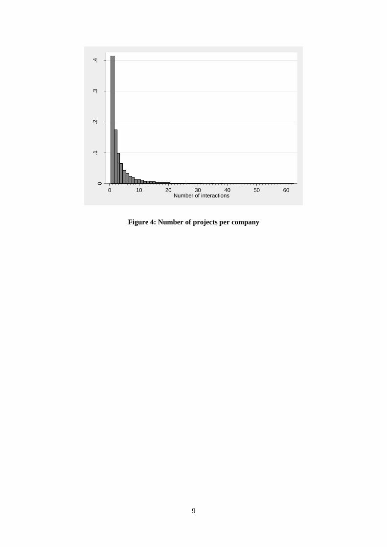
Figure 4 displays a histogram of the number of times each company interacted with FhG, in order to

assess the companies’ tendency to return to FhG over time.10

42% of all companies interact with FhG

only once. Another 17.5% return do so twice, and 9.9% have three interactions with Fraunhofer. The

remaining 30.6% interact with FhG more than three times. The fact that most companies in the data

interact once or twice with Fraunhofer supports the idea that it has a broad impact in the business

sector: FhG does not support a small number of specific companies, but instead supports thousands of

companies throughout the German economy with its knowledge. At the same time, a smaller part of

FhG’s client companies seem to form long-lasting relationships involving many interactions.

9 The average payment year was weighted by the share of the total paid in each year.

10 This analysis is restricted to the subset of the FhG data for which the client was identified as an MIP company.

Some care must be taken in the interpretation of this data, as the group of unidentified companies might include

subsidiaries (or similar) of MIP companies. As such, these statistics should be seen as lower limit estimates.

Multiple interactions may constitute independent projects, or they might be direct follow-up projects, with the

two too difficult to differentiate. Fehler! Verweisquelle konnte nicht gefunden werden. has been truncated at

the 99th

percentile, 62 projects. The true maximum goes up to 1050 projects (31 firms are found to have engaged

FhG for more than 100 projects).

0.2

.4.6

.81

Cu

mula

tive

dis

trib

utio

n

0 100 200 300 400 500Project Cost (tho. Eur)

9

Figure 4: Number of projects per company

0.1

.2.3

.4

Sha

re o

f firm

s

0 10 20 30 40 50 60Number of interactions

10

2.1.1 Project descriptions

To gain some insight into the goals and organization of FhG projects, a keyword analysis was

performed based on the short project descriptions available in the database. Table 1 lists the 20 most

common harmonized keywords in the project descriptions.11

They show that FhG projects cover the

full range, from studies and analysis to development, application and implementation. It is unlikely for

the impact of FhG projects to be constant across all these different types of projects. However, the

broad nature of the project descriptions limits the inference to be made. In the multivariate analysis,

we differentiate between projects whose description indicates a clear intent to implement whatever is

in the focus of the project (a technology, product, process, etc.) and those that indicate no such

intention of practical implementation. This allows us to assess whether projects further downstream

have an impact that differs from more upstream, abstract projects.12

Table 1: Project keywords

Rank Term No. of

projects

Share of

projects

Rank Term No. of

projects

Share of

projects

1 Development 6906 5.27% 11 Creation 1363 1.04%

2 Analysis 5348 4.08% 12 Feasibility 1354 1.03%

3 Study 4366 3.33% 13 Process 1336 1.02%

4 System 2481 1.89% 14 Application 1308 1.00%

5 Manufacturing 1776 1.35% 15 Technology 1248 0.95%

6 Supply 1740 1.33% 16 Structure 1112 0.85%

7 Project 1713 1.31% 17 Concept 1077 0.82%

8 Optimization 1687 1.29% 18 Simulation 1064 0.81%

9 Evaluation 1665 1.27% 19 Implementation 1059 0.81%

10 Test 1621 1.24% 20 Phase 1038 0.79%

11

Descriptions were short: the average description is 7 words long, and 90% of descriptions consist of 14 words

or less. Keywords in the descriptions were translated from German and harmonized. Common words as well as

brands and any identifying information have been removed from the data. 12

To achieve this, we developed and applied the following key: Projects were deemed “implementative” when

they included words indicating a change or development, such as “adapt”, “build”, “create”, “construct”,

“develop”, “improve”, “innovate”, “integrate”, “intervene”, “install”, “manufacture”, “modify”, “realize”,

“restructure”.

11

2.2 Variables

In this section, we describe the variables used in the analysis (described in Table 2). This includes the

variables that measure the interaction with Fraunhofer, the various outcomes and controls.

Interaction with Fraunhofer

The key explanatory variable of the study captures whether the company interacted with FhG. As

many projects in the database involve little or no payment to FhG, indicating that they are small in

size, a payment threshold needs to be defined to indicate when projects are of significant size.13

At the

same time, the project data needs to be transposed onto the company-year framework of the MIP.

Therefore, the project data was aggregated to the money paid to FhG for each company in each year.

As most companies are involved in one interaction at a time, this is not a strong assumption to make.14

A significant interaction was then defined as making a total payment of €13,000 or more to Fraunhofer

over the course of a given year.15

We name this variable FHG_INT. We also define a broader

interaction indicator, FHG, that takes value 1 if the company ever interacted with FHG over the

timeframe of the data. Lastly, we define FHG_AMOUNT to capture the size of the annual payment

made to FhG.

Outcomes

We approach the characterization of the effect of interaction with FhG on companies from different

perspectives. First, companies might be able to grow larger as a result of their interactions. The size of

the company is measured by sales (TURNOVER; million EUR) and by employee headcount

(EMPLOYEES). Second, implementing technology with support from FhG might be an efficient way

to increase productivity. To capture that, we calculate added value per employee (ADDVAL). Third,

Fraunhofer might support companies in the development and commercialization of their own

innovative products and processes. We capture these in a direct way through the share of sales

stemming from new or improved products introduced by the company (INNOSALES). Additionally,

13

A small minority of projects involved negative payment, i.e. money going from Fraunhofer to the firm. 14

In 64% of cases in which an MIP company interacts with FhG, there is only one interaction in that year. In

18% of cases there are two, and three or more only in 10% of cases. 15

The Fraunhofer database lists payments made by year. While these could in principle occur at any point after

starting a project, payments are typically made in the year after the project is started. Given the fact that the

median project lasts one year, this means that payments can be used as a proxy for Fraunhofer activity in that

time. A threshold of €13,000 was chosen to eliminate projects that are too small in scale to show a significant

impact on company performance indicators, and approximates the median payment made by MIP companies to

Fraunhofer in a given year, taking the total payment across all projects in which the company is involved into

account. In the robustness checks, we show that this definition holds up even under stricter definitions of an

interaction.

12

measures of average employee cost (CPE) and the share of employees with tertiary education

(EMP_HIGHED) capture any changes in company strategy with regard to innovation and R&D by

tracing changes in the composition of the workforce.

Table 2: Variable definitions

Name Source Description

Interaction with Fraunhofer FHG FhG data Binary 1 if company ever paid at least €13,000 to FhG

FHG_AMOUNT FhG data Numeric Payment made by company to FhG in year (€

k), taking all projects in which the company is

involved into account

FHG_INT FhG data Binary 1 if company paid at least €13,000 to FhG in

year

Outcomes TURNOVER MIP Numeric Turnover of company in year (€ million)

EMPLOYEES MIP Numeric Number of employees in year

ADDVAL MIP Numeric Added value per employee (€ million)

INNOSALES MIP Numeric Share of sales stemming from new or improved

products

CPE MIP Numeric Average employee cost (€ k)

EMP_HIGHED MIP Numeric Share of employees with tertiary education

Controls RD_INT MIP Numeric R&D expenditures scaled by turnover (ratio)

AGE Creditreform Numeric Years since company’s founding

GROUP MIP Binary 1 if company is member of a corporate group

EXPORT MIP Binary 1 if company indicates plans to export in year

EAST MIP Binary 1 if company is located in former East Germany

SIZE_(SMALL,

_MEDIUM, _LARGE)

MIP Binary Categoric indicator of company size. Small: up

to 49 employees. Medium: 50-249 employees.

Large: 250+ employees.

Sector MIP Categoric Categoric indicator: 21 sectors (see Table 4)

Year MIP Categoric Categoric indicator: calendar year

Controls

The analysis aims to estimate the effect of interacting with FhG on company performance. However,

certain factors need to be held constant. The degree to which a company can profit from interacting

with FhG is likely to be a function of internal R&D capacities (Cohen and Levinthal, 1990). To

control for this, we include a measure of in-house R&D intensity (RD_INT, R&D expenditures scaled

by turnover). Likewise, R&D intensity is expected to play an important role in selection for

Fraunhofer interaction, as companies with more innovation-focused strategies are more likely to have

projects with FhG.

We also include a number of more general indicators that capture the competitive situation of the

company. These include the company’s age (AGE) and a dummy indicating whether or not the

company exports (EXPORT). Additionally, we control for broad economic differences within

Germany by including a dummy that takes value 1 if the company is located in former East Germany

13

(EAST), and control for broad differences in company size through the inclusion of three company

size categories16

(SIZE_SMALL, SIZE_MEDIUM, and SIZE_LARGE). We further control for the

economic activities of the company through the inclusion of 21 broad sector indicators and include

year fixed effects to account for shared macroeconomic trends.

Company-level descriptives

Table 3 compares the outcome and control variables for companies that interacted or did not interact

with Fraunhofer in the project database. Table 4 shows the same for sector distribution. As shown in

the upper panel of Table 3, 6% of company-year observations in the MIP are found to contain

interactions with Fraunhofer. On average, a year in which a company paid money to FhG involves a

payment of approximately €37,000.

Companies that interact with FhG through projects are significantly (p<0.01, two-sided t-test) larger in

terms of turnover and employees. The difference is strong, approximating a tenfold size differential.

This is reflected in the company size categories: whereas 14% of companies that did not interact with

FhG are classified as large, 54% of the companies that do are large companies. At the same time,

companies that engage with FhG generate more sales from new or improved products (18% versus

6%). They also seem to be more productive, as added value per employee is approximately 20%

higher among companies that interact with FhG than among those that do not. Lastly, companies that

interact with FhG report higher average labor costs per employee (47.49 versus 35.22 € k) and a

higher share of employees with higher education (30% versus 20%). A similar pattern emerges in

terms of the controls: FhG companies are more R&D-intensive (10% compared to 3%), tend to be

older (37 years versus 28), are more likely to export their products (45% versus 25%), and are more

likely to be part of a group (68% versus 52%). FhG companies are more likely to be situated in former

West Germany than in former East Germany.

Taken together, these descriptive differences underline the importance of accounting for positive

selection bias in the empirical analysis. If left uncontrolled for, the impact of interacting with

Fraunhofer will be biased upwards.

16

Small: up to 49 employees. Medium: 50-249 employees. Large: 250+ employees. In estimations not related to

size, we control for company size by including the number of employees as a control variable.

14

Table 3: Company summary statistics

Total By Fraunhofer interaction

Interacted Did not interact Difference

Mean St. Dev Obs. Mean Obs. Mean Obs.

Interaction with FhG

FHG 0.06 0.24 198385 1.00 17103

FHG_INT 0.02 0.14 198385 0.24 17103

FHG_AMOUNT 3.23 53.80 198385 37.23 17103

Outcomes

TURNOVER 199.00 3593.82 131822 906.95 11239 133.02 120583 -773.93***

EMPLOYEES 531.56 7253.71 191065 2735.27 16571 322.28 174494 -2412.99***

INNOSALES 0.07 0.17 112029 0.18 7734 0.06 104295 -0.12***

ADDVAL 0.10 0.38 61955 0.12 5641 0.10 56314 -0.02***

CPE 36.23 17.16 77831 47.49 6376 35.22 71455 -12.27***

EMP_HIGHED 0.21 0.25 99873 0.30 8163 0.20 91710 -0.10***

Controls

RD_INT 0.04 0.58 77974 0.10 6989 0.03 70985 -0.07***

AGE 29.08 32.27 190804 37.44 16707 28.28 174097 -9.16***

EXPORT 0.27 0.44 198385 0.45 17103 0.25 181282 -0.20***

GROUP 0.54 0.50 198385 0.68 17103 0.52 181282 -0.16***

EAST 0.33 0.47 198385 0.27 17103 0.34 181282 0.07***

Company Size

SIZE_SMALL 0.56 0.50 191065 0.20 16571 0.59 174494 0.39***

SIZE_MEDIUM 0.27 0.44 191065 0.26 16571 0.27 174494 0.01**

SIZE_LARGE 0.17 0.38 191065 0.54 16571 0.14 174494 -0.40***

Notes: Firm-years. Difference: outcome of two-sided t-test. Stars indicate significance level of t-statistic. ***(,**,*): p <

0.01(,0.05, 0.10). Interaction with Fraunhofer: split made along having ever had Fraunhofer project between 1997 and 2014

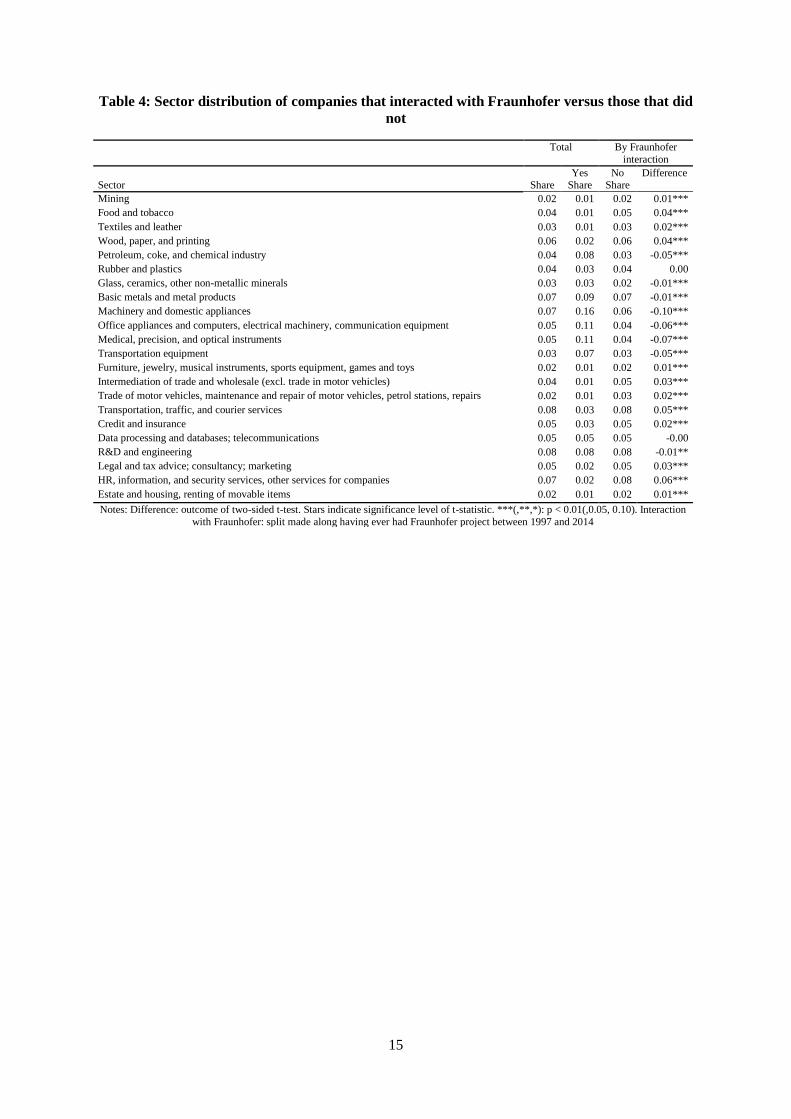
Table 4 shows the sector distribution of all companies, whether they interacted with FhG or not.

Companies interacting with FhG are more likely to be situated in medium and high-tech

manufacturing industries (specifically, petroleum and chemical industry, machinery and domestic

appliances, electrical machinery, communication equipment, instruments, and automotive), and less

likely to be active in low-tech manufacturing or service industries. The multivariate analysis needs to

correct for these differences in the composition of the samples for companies that have interacted with

FhG (FhG companies) and those that have not (non-FhG companies).

15

Table 4: Sector distribution of companies that interacted with Fraunhofer versus those that did

not

Total By Fraunhofer

interaction

Yes No Difference Sector Share Share Share

Mining 0.02 0.01 0.02 0.01***

Food and tobacco 0.04 0.01 0.05 0.04***

Textiles and leather 0.03 0.01 0.03 0.02***

Wood, paper, and printing 0.06 0.02 0.06 0.04***

Petroleum, coke, and chemical industry 0.04 0.08 0.03 -0.05***

Rubber and plastics 0.04 0.03 0.04 0.00

Glass, ceramics, other non-metallic minerals 0.03 0.03 0.02 -0.01***

Basic metals and metal products 0.07 0.09 0.07 -0.01***

Machinery and domestic appliances 0.07 0.16 0.06 -0.10***

Office appliances and computers, electrical machinery, communication equipment 0.05 0.11 0.04 -0.06***

Medical, precision, and optical instruments 0.05 0.11 0.04 -0.07***

Transportation equipment 0.03 0.07 0.03 -0.05***

Furniture, jewelry, musical instruments, sports equipment, games and toys 0.02 0.01 0.02 0.01***

Intermediation of trade and wholesale (excl. trade in motor vehicles) 0.04 0.01 0.05 0.03***

Trade of motor vehicles, maintenance and repair of motor vehicles, petrol stations, repairs 0.02 0.01 0.03 0.02***

Transportation, traffic, and courier services 0.08 0.03 0.08 0.05***

Credit and insurance 0.05 0.03 0.05 0.02***

Data processing and databases; telecommunications 0.05 0.05 0.05 -0.00

R&D and engineering 0.08 0.08 0.08 -0.01**

Legal and tax advice; consultancy; marketing 0.05 0.02 0.05 0.03***

HR, information, and security services, other services for companies 0.07 0.02 0.08 0.06***

Estate and housing, renting of movable items 0.02 0.01 0.02 0.01***

Notes: Difference: outcome of two-sided t-test. Stars indicate significance level of t-statistic. ***(,**,*): p < 0.01(,0.05, 0.10). Interaction

with Fraunhofer: split made along having ever had Fraunhofer project between 1997 and 2014

16

3 Identification strategy

Estimating the causal effects of project interactions with Fraunhofer institutes can mainly be

accomplished by regression techniques. Estimating the causal effect, however, is not straightforward

because of selection on unobservables and endogeneity. Furthermore, treatment (i.e. research projects

with Fraunhofer) is time-dependent in our setting, which can imply that the causal effect accumulates

over time (Robins et al., 2000; Azoulay, 2009). This section describes the methods employed in this

study to mitigate these statistical issues. The nontechnical reader can skip this section and move on to

the results.

If we abstract from the time dependence a simple model of the relationship between the company

performance yit and the cooperation variable 𝐹𝐻𝐺_𝐼𝑁𝑇𝑖𝑡 , this can be written as follows:

yit = xitβ + FHG_INTitδ + uit (1)

where xit is a vector of control variables and uit is a structural error term. δ is the central parameter of

interest and measures how the interaction variable affects company performance. Commissioning

research projects from Fraunhofer institutes, however, is not randomized, but will depend on a process

of mutual selection. If the factors governing the selection process can be sufficiently controlled for in

xit ,δ can be structurally identified by regular panel data models. But if selection is based on (time-

varying) unobservables, the estimates δ will generally be biased, because the central identification

condition that uit is uncorrelated with any of the vector of observed variables in 1, … T (strict

exogeneity) will not be met.

An often discussed case is when uit includes unobservable capabilities of the company. This variable

will be very likely to be correlated with the interaction variable, because more capable companies will

are more likely to self-select for collaborative projects and in turn will be more likely to be selected by

the Fraunhofer institutes. The capabilities are likely to be largely constant over time. If this is the case,

we can control for the unobserved company-specific capabilities by including a company-level fixed

effect (i.e. intercept) in equation (1).

However, if the company capabilities are time-varying, including fixed effects in (1), this does not

prevent a potential upward bias in the estimate of δ in (1). To prevent that, we need to identify δ from

exogenous variation in the interaction with Fraunhofer induced by instrumental variables.

Unfortunately, finding appropriate instrumental variables is difficult. Recently, Lewbel (2012) has

demonstrated how heteroscedasticity can help to generate instrumental variables. Specifically, suppose

our structural model takes the following form:

17

yit = xitβ + FHG_interactitδ+uit

FHG_interactit = xitζ + yitϑ + vit(2)

Unless ϑ = 0 the model is fully simultaneous and the performance equation cannot be consistently

estimated by regular regression techniques. Lewbel (2012) proved that for some vector zit if

cov(xit, uit2 ) ≠ 0, cov(xit, uit

2 ) ≠ 0, and cov(zit, uitvit) = 0, the system can be consistently identified.

The first two assumptions mean that heteroscedasticity exists in the error terms while the second

assumption is the pendant to a more conventional exogeneity assumption. To see why

heteroscedasticity can identify our effects, we define

zit = (xit − xt̅)ϵ (3)

where ϵ is the residual from reduced form regression of FHG_interactit on the exogenous regressors

xit. ϵ is structurally identified because the parameters in the reduced form regression can always be

consistently estimated (Wooldridge, 2002). These residuals furthermore have zero covariance with xit

by construction. However, the element-wise products with the regressors will not be zero throughout.

Furthermore, the elements will be the larger in absolute terms the larger the heteroscedasticity is.

Thus, the degree of heteroscedasticity is directly proportional to the correlation between the generated

instruments zit and the endogenous company performance measure, which can provide explanatory

power of the generated instruments. In order for the variation in the instruments to be exogenous,

Lewbel (2012) shows that condition cov(zit, uitvit) = 0 needs to hold. This assumption is technical,

but Lewbel (2012) shows that it generally holds if the error term can be written in an error-component

form. While the Lewbel result is more general, in our case if we are willing to assume that selection

occurs on unobservable company capabilities, we can rewrite the error-term as uit = capabilitπ + eit,

where eit is assumed to be an uncorrelated random error. The importance of the Lewbel result is that

our reasoning on why endogeneity exists leads directly to an error-component model, for which the

exogeneity assumption cov(zit, uitvit) = 0 automatically holds. Thus, the results based on Lewbel

(2012) provide a means to construct a valid instrumental variable for the likelihood that a company

will interact with Fraunhofer.

A separate issue from the econometric model described by Eq. (1) is that this specification assumes

that only contemporaneous Fraunhofer interactions have an effect on company performance. This is a

strong assumption, because past interactions may also have time-persistent effects, suggesting that

these may accumulate over time (Azoulay et al., 2009). A natural approach is thus to model the causal

interaction effect as a distributed lag model:

yit = xitβ + γ ∑ wittτ=1 FHG_interactit−τ + uit (4)

18

Two problems emerge when trying to estimate Eq. (4): First, the vector of weights is unknown.

Second, if past levels of the interaction variable affect the current levels of the exogenous regressors,

estimating Eq. (4) cannot generally be estimated without bias when past regressors affect later

treatment. A solution to both problems has been provided by Robins (1999) who introduces the

Sequential Conditional Independence Assumption (SCIA), which means that the contemporaneous

cooperation is independent of company performance, conditional on a one-period lag of the

interactions, the contemporaneous vector xit and a one-period lag of any other observable variables

affecting selection, zit−1. Robins (1999) shows that under SCIA, the weights in Eq. (4) are given by

the following formula:

wit =1

∏ P(FHG_interactiτ|FHG_interact̃ iτ−1,ziτ−1,xiτ)tτ=1

(5)

where FHG_interact̃iτ−1 represents a distributed lag of past interactions. Because of the structure of

the weights, this method is called Inverse Probability of Treatment Weights (IPTW) and has originated

from bio-statistics but recently has been applied also in economics. Azoulay et al. (2009) make the

point that the probabilities P(FHG_interactiτ|FHG_interact̃iτ−1, ziτ−1, xiτ) could vary strongly among

companies in the event that time-varying confounders are strongly associated with interaction, and

note that this could lead to large outliers in wit. Therefore, they propose using the stabilized weight:

𝑠wit =∏ P(FHG_interaciτ|FHG_interact̃ iτ−1,xiτ)t

τ=1

∏ P(FHG_interaciτ|FHG_interact̃ iτ−1,ziτ−1,xiτ)tτ=1

(6)

The probabilities in Eq. (6) can be estimated from the data from simple probability models such as

logistic or probit regressions (see Table 5). Based on the estimated weights all terms in Eq. (4) can be

derived and the regression can be estimated.

In our analysis, we will present various types of regressions. We will start with simple pooled OLS

models, which are likely to be biased due to selection. Then we will try to overcome this bias by

introducing fixed effects, IV models based on Lewbel instruments, and IPTW estimators.

19

4 Results

Determinants of interaction

Before describing the impact of Fraunhofer interactions on companies, it is worth exploring the

process of selection for the interaction. Table 5 displays selection estimates with and without time-

varying confounders. The results in column 1 confirm that interaction with FhG is strongly determined

by past payments: at the mean, having interacted with FhG in the year before increases the probability

of interaction by 30 percentage points, compared to a base probability of 2.6%. Company size is also a

strong predictor of interaction. Compared to small companies, medium companies are 19% more

likely to interact with FhG, while large companies are 50% more likely to do so. Exporting companies

are 11% more likely to interact with FhG than non-exporting companies. The other confounders, while

statistically significant, are less strong predictors: with all other factors constant, a 1% increase in

R&D intensity corresponds to a 0.06% increase in the probability of interacting with FhG, and a 1%

increase in R&D stock corresponds to a 0.19% increase. Companies located in former East Germany

are 3.8% more likely to interact.

This analysis thus confirms the descriptive statistics: large competitive companies are the most likely

to interact with Fraunhofer. In order to not overestimate the effect of interacting with Fraunhofer, we

need to correct for this selection through econometric techniques. One such technique involves

calculating IPTW weights.

Table 5: Probability of interacting with Fraunhofer

(1) (2)

FHG_INT

Denominator Numerator

𝐹𝐻𝐺_𝐼𝑁𝑇𝑡−1 4.286*** 4.721***

(0.098) (0.092)

𝑅𝐷_𝐼𝑁𝑇𝑡−1 0.059**

(0.023)

𝑅𝐷_𝐼𝑁𝑇_𝑆𝑇𝑂𝐶𝐾𝑡−2 0.064***

(0.022)

𝐸𝑋𝑃𝑂𝑅𝑇𝑡−1 0.442***

(0.083)

𝐹𝐼𝑅𝑀_𝑀𝐸𝐷𝐼𝑈𝑀𝑡−1 0.798***

(0.104)

𝐹𝐼𝑅𝑀_𝐿𝐴𝑅𝐺𝐸𝑡−1 1.954***

(0.104)

𝑙𝑛(𝐴𝐺𝐸 + 1) 𝑡−1 -0.031 0.139***

(0.042) (0.043)

𝐺𝑅𝑂𝑈𝑃𝑡−1 -0.102 0.208**

(0.087) (0.083)

𝐸𝐴𝑆𝑇𝑡−1 0.201** -0.079

(0.083) (0.079)

Intercept -5.587*** -5.966***

(0.421) (0.408)

Observations 64232 64232

Pseudo R-squared 0.463 0.429

Joint significance test of time-variant variables 458.251

included: 21 sector indicators and 17 year indicators. Cluster-robust

standard errors in parentheses. * p<0.10, ** p<0.05, *** p<0.01

20

FhG interaction and company performance

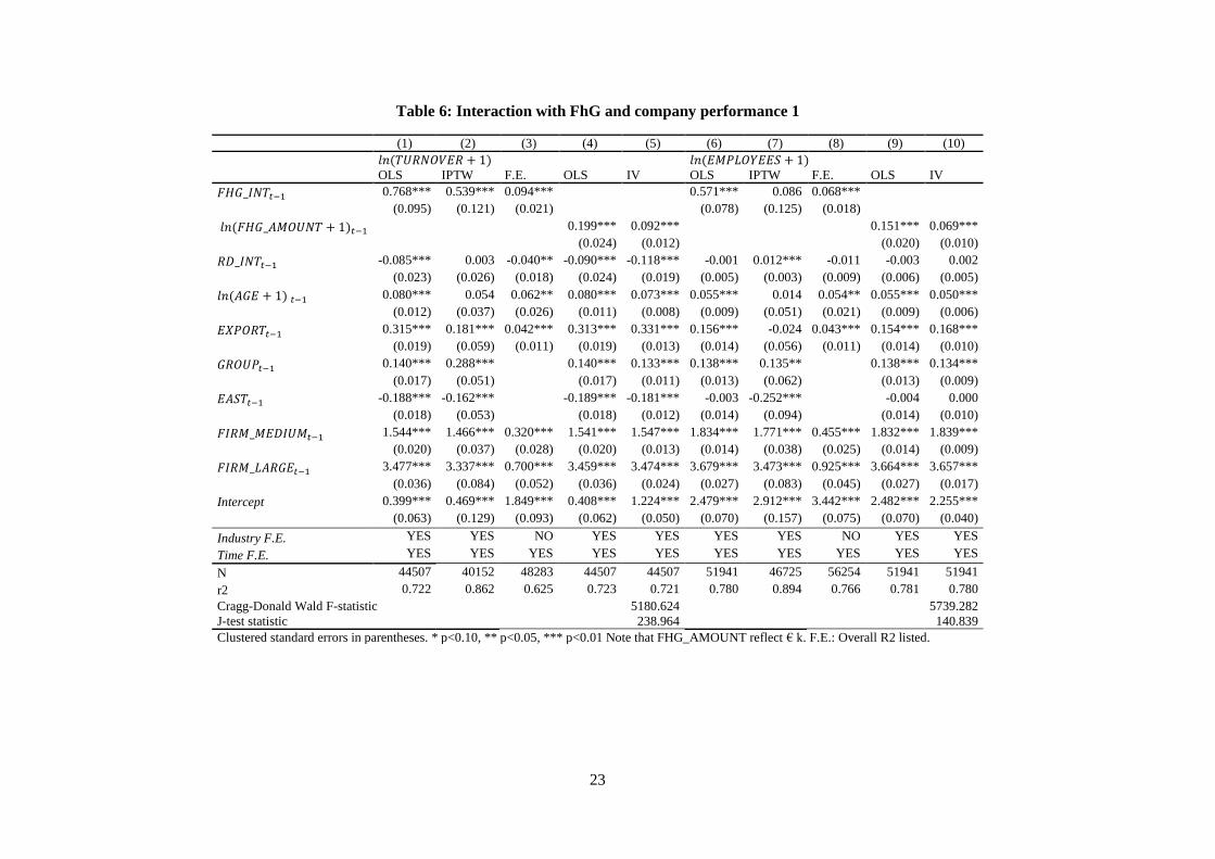
Tables 6, 7 and 8 provide the main results of the paper through estimates of the relationship between

an interaction with FhG and company size (turnover and employees, Table 6); productivity and

innovative sales (Table 7); and the composition of the labor force (average employee cost and share of

highly educated employees, Table 8). Each outcome is estimated by 5 methods. The first is an OLS

model including a dummy indicating that the company interacted with FhG in the previous period.

Second is the same model including IPTW weights, which should account for selection based on

observable characteristics such as company size, R&D investment and past treatment. The third is a

model including the same dummy and company-specific intercepts to account for constant unobserved

company effects. The final two models are an OLS exploiting the volume of treatment instead of a

treatment dummy, and the same model where the treatment volume is instrumented through

heteroscedasticity-based instruments employing the Lewbel (2012) technique. In each model, we hold

company size constant (in the models taking company size as dependent, we include broad indicators

as to whether the company is a small, medium or large company. In the other models, we include

employee headcount as an explanatory factor), as well as R&D intensity, company age, whether the

company exports, whether the company is part of a group, and whether the company is situated in

former East Germany. All explanatory variables, including the interaction indicator, are lagged with

one year. Hence, the interpretation of the key coefficient is the impact one year after treatment.

Below we present the main conclusions for each outcome. We note that the OLS and IPTW results,

compared to those from the fixed effects models, confirm the presence of strong selection effects that

cannot be completely controlled for. The coefficients for all OLS and IPTW specifications are much

larger than the fixed effects estimates, and likewise the instrumented effects of volume are much lower

than those shown by the OLS specification. The unrealistic magnitude shown by the OLS models (for

instance, the OLS estimate of the effect of FhG interaction in the previous year is a 115% increase in

turnover) underscores the importance of correcting for selection. Therefore, we consider the (most

conservative) fixed effect and IV estimates to be our main result.

Turnover (Table 6, columns 1-5): The OLS estimate of 77% decreases to 54% once the likelihood of

treatment as calculated through IPTW has been taken into account. However, the fixed effects model

shows a lower, but still significant, effect of 9.4%. Likewise, the estimated elasticity of payment to

FhG with regard to turnover of 20% in the OLS specification sinks to 9.2% once it has been

instrumented for. Even though the specifications decrease the magnitudes of the effects, they remain –

economically and statistically – highly significant: our most conservative estimates indicate that an

interaction with Fraunhofer is followed by a 9% increase in turnover the following year.

21

Employees (Table 6, columns 6-10): Similar results hold for the number of employees in the company

as measure of company size. The OLS estimates are very large, at an impact of 57% when considering

an interaction indicator (column 6) and an elasticity of 15% when considering payment volume

(column 9). When correcting for selection through the use of IPTW, the effect is still large (8.6%), but

becomes statistically insignificant. This may relate to the inclusion of company size indicators in the

calculation of the weights (even though the size indicators constitute broad categories). Nevertheless,

in the fixed effects model, we estimate a statistically and economically significant impact of 6.8% after

an interaction, and an elasticity of payment volume to employees of 6.9%.

Value added (Table 7, columns 1-5): The strong effects of interacting with FhG on company size are

weaker when considering added value per employee as an outcome measure. Whereas the OLS and

IPTW specifications show statistically significant increases in added value following an interaction –

around 1.6% and 2.5%, respectively – and whereas an elasticity of 0.4% of payment volume to added

value is found, the fixed effects model does not find a statistically significant relationship.

Nevertheless, the instrumental variable specification also results in a statistically significant (albeit

only weakly so) elasticity of some 0.1%.

New or improved product sales (Table 7, columns 6-10): The impact that interacting with FhG has on

new or improved sales is somewhat ambiguous. Whereas the OLS indicates an effect of 9.7%, the

IPTW as well as fixed effect specifications show very low and statistically insignificant impacts (1.4%

and 0.4%, respectively). This indicates that most of the OLS impact is due to selection effects.

Nevertheless, the IV model shows a statistically significant semi-elasticity of FhG payment volume on

new or improved sales of 0.8%. This leads to the conclusion that while the impact of an average

interaction is not statistically significant, it increases when projects become larger.

Average employee cost (Table 8, columns 1-5): The results pattern found for new or improved product

sales is also found in average employee cost: while the OLS (9.6%) and IPTW (14.1%) models show a

large and significant impact, this is mainly due to selection effects, as the fixed effects model shows an

insignificant and small impact (1.5%). Nevertheless, the impact of interaction increases as payment

volume grows larger, with elasticities of 2.5% in the OLS specification and 1.5% in the IV model.

Share of highly educated employees (Table 8, columns 6-10): Similarly, the share of highly educated

employees does seem to respond to interaction with FhG in the OLS specification (with an impact of

9.4%) and the IPTW models (8.4%). However, at least some of the effect shown by the IPTW model

seems to be due to selection on unobservable company effects, and the fixed effects model does not

support a positive impact. At the same time, the impact increases with project size, with estimated

elasticities by the OLS of 2.4% and 1.4% according to the IV specification.

The analysis yields valuable insights on the effects of interacting with FhG. While we cannot claim to

have accounted for all endogeneity issues, the fixed effect models and heteroscedasticity-based

22

instrumentation of payment volume show robust positive correlations between FhG interactions and

company size. While the effect of the average interaction on added value, innovative performance and

innovative strategy cannot be confirmed through fixed effects models, the IV models support the ideas

of positively significant elasticities between more intense interaction with FhG and added value,

innovative performance and innovative strategy.

23

Table 6: Interaction with FhG and company performance 1

(1) (2) (3) (4) (5) (6) (7) (8) (9) (10)

𝑙𝑛(𝑇𝑈𝑅𝑁𝑂𝑉𝐸𝑅 + 1) 𝑙𝑛(𝐸𝑀𝑃𝐿𝑂𝑌𝐸𝐸𝑆 + 1)

OLS IPTW F.E. OLS IV OLS IPTW F.E. OLS IV

𝐹𝐻𝐺_𝐼𝑁𝑇𝑡−1 0.768*** 0.539*** 0.094***

0.571*** 0.086 0.068***

(0.095) (0.121) (0.021)

(0.078) (0.125) (0.018)

𝑙𝑛(𝐹𝐻𝐺_𝐴𝑀𝑂𝑈𝑁𝑇 + 1)𝑡−1 0.199*** 0.092*** 0.151*** 0.069***

(0.024) (0.012) (0.020) (0.010)

𝑅𝐷_𝐼𝑁𝑇𝑡−1 -0.085*** 0.003 -0.040** -0.090*** -0.118*** -0.001 0.012*** -0.011 -0.003 0.002

(0.023) (0.026) (0.018) (0.024) (0.019) (0.005) (0.003) (0.009) (0.006) (0.005)

𝑙𝑛(𝐴𝐺𝐸 + 1) 𝑡−1 0.080*** 0.054 0.062** 0.080*** 0.073*** 0.055*** 0.014 0.054** 0.055*** 0.050***

(0.012) (0.037) (0.026) (0.011) (0.008) (0.009) (0.051) (0.021) (0.009) (0.006)

𝐸𝑋𝑃𝑂𝑅𝑇𝑡−1 0.315*** 0.181*** 0.042*** 0.313*** 0.331*** 0.156*** -0.024 0.043*** 0.154*** 0.168***

(0.019) (0.059) (0.011) (0.019) (0.013) (0.014) (0.056) (0.011) (0.014) (0.010)

𝐺𝑅𝑂𝑈𝑃𝑡−1 0.140*** 0.288*** 0.140*** 0.133*** 0.138*** 0.135** 0.138*** 0.134***

(0.017) (0.051) (0.017) (0.011) (0.013) (0.062) (0.013) (0.009)

𝐸𝐴𝑆𝑇𝑡−1 -0.188*** -0.162*** -0.189*** -0.181*** -0.003 -0.252*** -0.004 0.000

(0.018) (0.053) (0.018) (0.012) (0.014) (0.094) (0.014) (0.010)

𝐹𝐼𝑅𝑀_𝑀𝐸𝐷𝐼𝑈𝑀𝑡−1 1.544*** 1.466*** 0.320*** 1.541*** 1.547*** 1.834*** 1.771*** 0.455*** 1.832*** 1.839***

(0.020) (0.037) (0.028) (0.020) (0.013) (0.014) (0.038) (0.025) (0.014) (0.009)

𝐹𝐼𝑅𝑀_𝐿𝐴𝑅𝐺𝐸𝑡−1 3.477*** 3.337*** 0.700*** 3.459*** 3.474*** 3.679*** 3.473*** 0.925*** 3.664*** 3.657***

(0.036) (0.084) (0.052) (0.036) (0.024) (0.027) (0.083) (0.045) (0.027) (0.017)

Intercept 0.399*** 0.469*** 1.849*** 0.408*** 1.224*** 2.479*** 2.912*** 3.442*** 2.482*** 2.255***

(0.063) (0.129) (0.093) (0.062) (0.050) (0.070) (0.157) (0.075) (0.070) (0.040)

Industry F.E. YES YES NO YES YES YES YES NO YES YES

Time F.E. YES YES YES YES YES YES YES YES YES YES

N 44507 40152 48283 44507 44507 51941 46725 56254 51941 51941

r2 0.722 0.862 0.625 0.723 0.721 0.780 0.894 0.766 0.781 0.780

Cragg-Donald Wald F-statistic 5180.624

5739.282

J-test statistic

238.964

140.839

Clustered standard errors in parentheses. * p<0.10, ** p<0.05, *** p<0.01 Note that FHG_AMOUNT reflect € k. F.E.: Overall R2 listed.

24

Table 7: Interaction with FhG and company performance 2

(1) (2) (3) (4) (5) (6) (7) (8) (9) (10)

𝑙𝑛(𝐴𝐷𝐷𝑉𝐴𝐿 + 1) 𝐼𝑁𝑁𝑂𝑆𝐴𝐿𝐸𝑆

OLS IPTW F.E. OLS IV OLS IPTW F.E. OLS IV

𝐹𝐻𝐺_𝐼𝑁𝑇𝑡−1 0.016*** 0.025*** 0.011

0.097*** 0.014 0.004

(0.006) (0.005) (0.007)

(0.013) (0.021) (0.010)

𝑙𝑛(𝐹𝐻𝐺_𝐴𝑀𝑂𝑈𝑁𝑇 + 1)𝑡−1

0.004*** 0.001*

0.024*** 0.008***

(0.001) (0.001)

(0.003) (0.002)

𝑅𝐷_𝐼𝑁𝑇𝑡−1 -0.006** -0.006** -0.000 -0.006** -0.010*** 0.017* 0.001 -0.002 0.017* 0.030***

(0.003) (0.003) (0.001) (0.003) (0.002) (0.010) (0.002) (0.002) (0.010) (0.008)

𝑙𝑛(𝐴𝐺𝐸 + 1) 𝑡−1 -0.001 -0.000 -0.004 -0.001 -0.001 -0.014*** -0.011 -0.021*** -0.014*** -0.014***

(0.001) (0.001) (0.004) (0.001) (0.001) (0.002) (0.007) (0.006) (0.002) (0.001)

𝐸𝑋𝑃𝑂𝑅𝑇𝑡−1 0.009*** 0.008*** -0.000 0.009*** 0.012*** 0.060*** 0.035*** 0.006 0.060*** 0.060***

(0.002) (0.003) (0.003) (0.002) (0.002) (0.004) (0.010) (0.004) (0.004) (0.003)

𝐺𝑅𝑂𝑈𝑃𝑡−1 0.006*** 0.006** 0.006*** 0.005*** 0.009*** 0.033*** 0.009*** 0.008***

(0.002) (0.003) (0.002) (0.002) (0.003) (0.010) (0.003) (0.002)

𝐸𝐴𝑆𝑇𝑡−1 -0.024*** -0.018*** -0.024*** -0.023*** 0.015*** 0.042* 0.015*** 0.015***

(0.002) (0.003) (0.002) (0.002) (0.003) (0.025) (0.003) (0.002)

𝑙𝑛(𝐸𝑀𝑃𝐿𝑂𝑌𝐸𝐸𝑆 + 1)𝑡−1 0.004*** 0.003*** -0.002 0.004*** 0.004*** 0.006*** -0.002 -0.001 0.005*** 0.005***

(0.001) (0.001) (0.004) (0.001) (0.001) (0.001) (0.003) (0.003) (0.001) (0.001)

Intercept 0.154*** 0.159*** 0.118*** 0.155*** 0.172*** 0.023** -0.047 0.122*** 0.025** 0.007

(0.016) (0.017) (0.023) (0.016) (0.011) (0.011) (0.030) (0.022) (0.011) (0.006)

Industry F.E. YES YES NO YES YES YES YES NO YES YES

Time F.E. YES YES YES YES YES YES YES YES YES YES

N 24734 23236 27282 24734 24734 38733 36569 42372 38733 38733

r2 0.148 0.200 0.001 0.148 0.146 0.178 0.384 0.032 0.179 0.174

Cragg-Donald Wald F-statistic

2382.897

3987.425

J-test statistic

101.641

167.188

Clustered standard errors in parentheses. * p<0.10, ** p<0.05, *** p<0.01 Note that FHG_AMOUNT reflect € k. F.E.: Overall R2 listed.

25

Table 8: Interaction with FhG and company performance

(1) (2) (3) (4) (5) (6) (7) (8) (9) (10)

ln(𝐶𝑃𝐸 + 1) 𝐸𝑀𝑃𝐻𝐼𝐺𝐻𝐸𝐷

OLS IPTW F.E. OLS IV OLS IPTW F.E. OLS IV

𝐹𝐻𝐺_𝐼𝑁𝑇𝑡−1 0.096*** 0.141*** 0.015

0.094*** 0.084*** 0.002

(0.018) (0.029) (0.012)

(0.010) (0.017) (0.005)

𝑙𝑛(𝐹𝐻𝐺_𝐴𝑀𝑂𝑈𝑁𝑇 + 1)𝑡−1

0.025*** 0.015***

0.024*** 0.014***

(0.005) (0.003)

(0.002) (0.002)

𝑅𝐷_𝐼𝑁𝑇𝑡−1 0.018 0.018 -0.001 0.018 0.042*** 0.040*** 0.056*** 0.007** 0.040*** 0.043***

(0.018) (0.020) (0.004) (0.018) (0.012) (0.011) (0.019) (0.003) (0.011) (0.010)

𝑙𝑛(𝐴𝐺𝐸 + 1) 𝑡−1 0.020*** 0.011 0.005 0.020*** 0.020*** -0.016*** -0.011 -0.011** -0.016*** -0.016***

(0.005) (0.018) (0.016) (0.005) (0.004) (0.002) (0.008) (0.005) (0.002) (0.001)

𝐸𝑋𝑃𝑂𝑅𝑇𝑡−1 0.137*** 0.120*** 0.015* 0.137*** 0.126*** 0.044*** 0.060*** -0.003 0.044*** 0.044***

(0.010) (0.017) (0.009) (0.010) (0.008) (0.004) (0.009) (0.003) (0.004) (0.003)

𝐺𝑅𝑂𝑈𝑃𝑡−1 0.013 0.058*** 0.013 0.010 0.005 0.001 0.005 0.006**

(0.010) (0.020) (0.010) (0.007) (0.004) (0.013) (0.004) (0.003)

𝐸𝐴𝑆𝑇𝑡−1 -0.215*** -0.356*** -0.215*** -0.222*** 0.045*** 0.065 0.045*** 0.046***

(0.010) (0.018) (0.010) (0.007) (0.004) (0.041) (0.004) (0.003)

𝑙𝑛(𝐸𝑀𝑃𝐿𝑂𝑌𝐸𝐸𝑆 + 1)𝑡−1 0.063*** 0.052*** 0.024* 0.063*** 0.069*** -0.012*** -0.015*** -0.021*** -0.018*** -0.011***

(0.003) (0.007) (0.013) (0.004) (0.002) (0.001) (0.004) (0.004) (0.002) (0.001)

Intercept 2.977*** 3.064*** 3.477*** 2.979*** 3.488*** 0.121*** 0.121** 0.332*** 0.124*** 0.293***

(0.040) (0.048) (0.076) (0.040) (0.030) (0.011) (0.050) (0.022) (0.011) (0.011)

Industry F.E. YES YES NO YES YES YES YES NO YES YES

Time F.E. YES YES YES YES YES YES YES YES YES YES

N 30629 27632 33342 30629 30629 37575 34554 40797 37575 37575

r2 0.255 0.859 0.050 0.256 0.254 0.435 0.924 0.059 0.436 0.435

Cragg-Donald Wald F-statistic 3526.526 3912.822

J-test statistic 211.546 122.611

Clustered standard errors in parentheses. * p<0.10, ** p<0.05, *** p<0.01. Note that FHG_AMOUNT reflect € k. F.E.: Overall R2 listed.

26

Effects over time

How long these effects persist is a relevant question. To gain more insights into this, we estimate the

following (OLS) model:

yit = FHGPAYi,t−1 + FHG_PAYi,t−2/t−4 + FHG_PAYi,t−5/t−7 + FHGi + TRENDt + FHGI ∗ TRENDT

+ Xt−1 + εit

This model allows us to compare differences in outcomes at 1 year after treatment, 2 to 4 years after,

and 5 to 7 years after. Systematic differences between companies that have or have not interacted with

FhG (FhG and non-FhG companies, respectively) are accounted for in the term FHG, and systematic

time trends are accounted for in TREND. Note that for FhG companies, TREND is set to zero after the

first interaction. Together with an interaction with FHG, TREND thus captures time trends for non-

FhG companies, and pre-treatment trends for FhG companies. This specification allows us to take into

consideration the effect of FhG and non-FhG companies from multiple perspectives. First, we can

trace the impact of an interaction over time by comparing the coefficients of FHG_INT as time goes

on. Second, we can calculate whether the effect is higher than where the company would be expected

to be, had it followed the trend just before treatment. Finally, this model allows us to explicitly

compare the trends followed by treated and untreated FhG companies (i.e. FhG companies after they

interacted, and had they not interacted – as predicted by the model) to non-FhG companies.

Table 9 shows the results of this specification. In all but two specifications (added value and average

employee cost), FhG companies perform systematically better than non-FhG companies. In two

specifications (turnover and average employee cost), FhG companies also follow a more positive trend

before treatment, compared to non-FhG companies. Turning to the post-interaction effects, the

strongest effects are observed for turnover and employees, which show positive coefficients up to 7

years after treatment. While the coefficients are largest in the first year after treatment, the effects

remain significant throughout the period. The share of new and improved product sales shows a

positive coefficient up to 4 years after treatment, but not after 5 years. EMP_HIGHED shows a

positive coefficient in the first year after treatment, but becomes insignificant again in the years after.

CPE and ADDVAL show no significant coefficients in this specification.

To ensure correct interpretation, this effect of interaction needs to be compared to the trend and level

of non-FhG companies and untreated FhG companies, respectively. Therefore, Table 10 provides

significance tests comparing the coefficient of FHG_INT with the projected trend (and level) of both

groups at 1, 3 and 6 years after interaction. Figure 5 provides a graphical illustration.

27

Panel A of Table 10 and Figure 5 confirm persistent large and statistically significant differences

between FhG companies and non-FhG companies. At virtually every point in time, the projected trend

and level of FhG companies is statistically significantly higher than those of non-FhG companies.

Panel B further shows that interacting FhG companies are significantly different from non-FhG

companies. However, this is only weakly statistically significant for added value per employee, where

the differences are small, and is not significant for average employee cost immediately after treatment.

Table 9: Interaction with FhG: Effect over time

(1) (2) (3) (4) (5) (6)

𝑙𝑛(𝑇𝑈𝑅𝑁𝑂𝑉𝐸𝑅 + 1) 𝑙𝑛(𝐸𝑀𝑃𝐿𝑂𝑌𝐸𝐸𝑆 + 1) 𝑙𝑛(𝐴𝐷𝐷𝑉𝐴𝐿 + 1) INNOSALES 𝑙𝑛(𝐶𝑃𝐸 + 1) EMP_HIGHED

𝐹𝐻𝐺_𝐼𝑁𝑇𝑡−1 0.425*** 0.307*** 0.004 0.029** 0.007 0.024**

(0.084) (0.069) (0.006) (0.013) (0.018) (0.010)

𝐹𝐻𝐺_𝑃𝐴𝑌𝑡−2,𝑡−4 0.158*** 0.136*** -0.004 0.031*** 0.022 0.013

(0.055) (0.043) (0.008) (0.012) (0.018) (0.009)

𝐹𝐻𝐺_𝑃𝐴𝑌𝑡−5,𝑡−7 0.217*** 0.165*** 0.008 0.019 0.026 0.006

(0.080) (0.062) (0.008) (0.015) (0.020) (0.010)

𝐹𝐻𝐺 0.276*** 0.255*** 0.007 0.068*** -0.010 0.075***

(0.069) (0.053) (0.005) (0.016) (0.022) (0.012)

𝑇𝑅𝐸𝑁𝐷 0.005 0.010** -0.001 0.002 -0.010*** -0.000

(0.007) (0.005) (0.001) (0.001) (0.002) (0.001)

𝑇𝑅𝐸𝑁𝐷 ∗ 𝐹𝐻𝐺 0.015** 0.006 0.001 -0.002 0.012*** 0.001

(0.007) (0.006) (0.001) (0.002) (0.003) (0.001)

𝑅𝐷_𝐼𝑁𝑇𝑡−1 -0.103*** -0.004 -0.007** 0.016* 0.014 0.037***

(0.028) (0.006) (0.003) (0.010) (0.017) (0.010)

𝑙𝑛(𝐴𝐺𝐸 + 1) 𝑡−1 0.081*** 0.056*** -0.001 -0.014*** 0.020*** -0.016***

(0.011) (0.008) (0.001) (0.002) (0.005) (0.002)

𝐸𝑋𝑃𝑂𝑅𝑇𝑡−1 0.293*** 0.133*** 0.008*** 0.058*** 0.133*** 0.041***

(0.019) (0.014) (0.002) (0.004) (0.010) (0.004)

𝐺𝑅𝑂𝑈𝑃𝑡−1 0.133*** 0.127*** 0.006*** 0.009*** 0.013 0.005

(0.017) (0.013) (0.002) (0.003) (0.010) (0.004)

𝐸𝐴𝑆𝑇𝑡−1 -0.186*** 0.001 -0.024*** 0.015*** -0.216*** 0.045***

(0.018) (0.014) (0.002) (0.003) (0.010) (0.004)

𝐹𝐼𝑅𝑀_𝑀𝐸𝐷𝐼𝑈𝑀𝑡−1 1.540*** 1.857***

(0.020) (0.013)

𝐹𝐼𝑅𝑀_𝐿𝐴𝑅𝐺𝐸𝑡−1 3.443*** 3.708***

(0.036) (0.025)

𝑙𝑛(𝐸𝑀𝑃𝐿𝑂𝑌𝐸𝐸𝑆 + 1)𝑡−1

0.003*** 0.003*** 0.059*** -0.016***

(0.001) (0.001) (0.004) (0.001)

Intercept 1.116*** 2.034*** 0.193*** 0.002 3.666*** 0.319***

(0.152) (0.116) (0.023) (0.027) (0.055) (0.025)

N 44445 52115 24734 38733 30629 37575

r2 0.739 0.812 0.149 0.184 0.258 0.442

included: 21 sector indicators and 17 year indicators. Clustered standard errors in parentheses. * p<0.10, ** p<0.05, *** p<0.01

Panel C shows the difference between companies that interacted with FhG compared to FhG

companies that did not interact but follow the predicted pre-interaction trend. The graphs show that

FhG companies grow after interaction and draw more of their sales from new products or services than

the projected trend would have indicated. These differences decrease over time, but remain statistically

significant for employees (and for turnover 4 years after interacting, but not 7 years after). The

analysis also shows an increase of approximately 3 percentage points in terms of new product sales,

which persists up to 4 years after treatment. After 5 years, it turns statistically insignificant but remains

similar in magnitude. An interaction with FhG coincides with an increase in the share of highly

28

educated employees of 2 percentage points, which does not persist over time. We find no statistically

significant differences between interacting FhG companies and the projected trend of these companies

for added value per employee and average employee cost.

These findings supplement the results concerning the immediate impact of interacting with FhG

shown in the previous section. We find persistent differences between companies that interacted with

FhG and their predicted pre-treatment path for turnover, employees, and new or improved product

sales. We find no persistent statistically significant differences for added value per employee, average

employee cost, and the share of employees with tertiary education.

Figure 5: Interaction with FhG over time: Graphical illustration

Table 10: Interaction with FhG over time: Significance tests

LN(TURNOVER+1) LN(EMPLOYEES+1) LN(ADDVAL+1) INNOSALES LN(CPE+1) EMP_HIGHED

t Coef S.E. Coef S.E. Coef S.E. Coef S.E. Coef S.E. Coef S.E.

Panel A: FhG companies compared to non-FhG

1 0.285*** (0.060) 0.251*** (0.047) 0.008* (0.004) 0.064*** (0.014) 0.012 (0.019) 0.076*** (0.010)

3 0.304*** (0.049) 0.243*** (0.038) 0.012*** (0.004) 0.058*** (0.010) 0.056*** (0.015) 0.078*** (0.008)

6 0.333*** (0.054) 0.230*** (0.042) 0.017*** (0.006) 0.048*** (0.009) 0.121*** (0.018) 0.082*** (0.009)

Panel B: Interacting FhG compared to non-FhG

1 0.695*** (0.097) 0.552*** (0.079) 0.011* (0.006) 0.096*** (0.018) 0.007 (0.024) 0.099*** (0.014)

3 0.418*** (0.068) 0.360*** (0.052) 0.006 (0.007) 0.094*** (0.015) 0.042* (0.022) 0.089*** (0.012)

6 0.461*** (0.077) 0.358*** (0.057) 0.020* (0.010) 0.077*** (0.017) 0.077*** (0.025) 0.083*** (0.012)

1

1.2

1.4

1.6

1.8

-2 -1 0 1 2 3 4 5 6 7Time

Turnover

2

2.2

2.4

2.6

-2 -1 0 1 2 3 4 5 6 7Time

Employees

.175

.18

.185

.19

.195

.2

-2 -1 0 1 2 3 4 5 6 7Time

Added Value per Employee

-.02

0

.02

.04

.06

.08

-2 -1 0 1 2 3 4 5 6 7Time

New Product Sales

3.55

3.6

3.65

3.7

-2 -1 0 1 2 3 4 5 6 7Time

Average Emp Cost

.3

.35

.4

-2 -1 0 1 2 3 4 5 6 7Time

High Ed Emp

Note: Interaction at t0

Fraunhofer Firms Non-Fraunhofer Firms

Projected Fraunhofer Trend

29

Panel C: Interacting FhG compared to non-interacting FhG

1 0.410*** (0.084) 0.301*** (0.069) 0.003 (0.006) 0.031** (0.013) -0.004 (0.018) 0.023** (0.001)

3 0.113* (0.060) 0.118** (0.047) -0.006 (0.008) 0.036*** (0.012) -0.013 (0.021) 0.010 (0.010)

6 0.128 (0.098) 0.128* (0.076) 0.003 (0.011) 0.030 (0.018) -0.045 (0.028) 0.001 (0.014)

Note: t: years after interaction. Panel A: FHG + t* TREND#FHG - t*TREND. Panel B: Coef reflects outcome of the relevant FHG_INT

coefficient + FhG - t*TREND. Panel C: FHG_INT - t* TREND#FHG. Significance stars reflect whether result is different from zero at p<0.1(,0.05,0.01): *(,**,***).

Robustness checks and extensions

Lastly, we perform several additional analyses to further explore the impact of interacting with FhG

and to test the validity of our results. The results are presented in Table 11.17

Panel A of Table 11 splits interactions into those that involve an implementation and those that do not

(see above for the definition). Whereas we find positive effects for both kinds for company size

(turnover and employees), we find a positive effect on added value per employee only when the

project involves implementing a change at the company. Thus, interacting with FhG seems to have an

effect on company efficiency only when projects are especially downstream and lead to real changes

in the organization.

Panel B explores the impact of interacting with FhG by considering the effect of first interactions

coupled with the effect of follow-on interaction. The results provide a strong indication that benefits

from interacting with FhG are concentrated in follow-on interactions. In consequence, it is important

for companies to build long-term relationships with FhG if they wish to reap the maximum benefits of

interacting with them.18

Panel C tests the robustness of the analysis to different definitions of interaction. As seen in the top

half of Panel C, which lists different payment thresholds for an interaction, the results are robust to

changes in the payment threshold. The sole exception is €50,000, which yields less statistically

significant results. The bottom half of Panel C shows the effects of interactions in different payment

ranges. Interactions involving payments of €0 to 5,000 generate no significant impact (the coefficient

of added value per employee is even negative). Payments between €5,000 and 10,000 and between

€10,000 and 50,000 generate similar impacts. However, those between €50,000 and 100,000 generate

some impacts, whereas interactions constituting a payment of €100,000 or more generate the greatest

impacts. This indicates that there are some nonlinearities with regard to the relationship between

project size and impact.

17

Due to space constraints, the results are restricted to fixed effects model estimates. 18

This effect should be interpreted with care, as it is difficult to distinguish separate, independent interactions

from multiple interactions within the context of a larger overarching project. Part of the larger effect of follow-

on interaction might therefore be that these firms are engaged in large projects that involve interaction with FhG

at multiple stages.

30

Panel D splits the samples into manufacturing and services sectors. The effects uncovered in the

present analysis in terms of company size are concentrated in manufacturing companies, in line with

the mission of FhG.

Panel E further splits the sample into three categories of company size: small (up to 49 employees),

medium (50-249 employees), and large (250+ employees). Whereas small companies do not

significantly benefit from interacting with FhG in terms of turnover, they do achieve employment

growth of around 8%. Medium and large companies, on the other hand, benefit more in terms of

turnover. The different effects observed here could indicate different projects pursued by small and

large companies, and a different role played by FhG in the development of each.

Panel F splits the results by company age, distinguishing young companies (10 years of age or less)

from older companies. While we find positive impacts on companies of all ages, the effects are

statistically more significant for older companies. In all likelihood, this is due to the relative lack of

young companies in interactions with FhG.

Table 11: Split estimates

LN(TURNOVER+1) LN(EMPLOYEES+1) LN(ADDVAL+1) INNOSALES LN(CPE+1) EMP_HIGHED

Panel A: By project implementation status

Yes 0.063** 0.044* 0.006** 0.011 -0.004 0.010*

(0.027) (0.023) (0.003) (0.012) (0.018) (0.006)

No 0.099*** 0.081*** 0.010 0.003 0.011 0.002

(0.027) (0.023) (0.008) (0.011) (0.014) (0.006)

Panel B: By repetition of interaction

First 0.004 0.016 -0.002 -0.002 0.019 0.000

(0.025) (0.019) (0.003) (0.014) (0.017) (0.006)

Follow-on 0.124*** 0.082*** 0.017* 0.007 0.011 0.001

(0.026) (0.023) (0.009) (0.013) (0.015) (0.005)

Panel C: By payment size threshold (€ k)

All 0.070*** 0.055*** 0.001 0.008 0.015 0.001

(0.017) (0.014) (0.004) (0.009) (0.013) (0.005)

5+ 0.093*** 0.065*** 0.006 0.013 0.019 -0.002

(0.018) (0.016) (0.005) (0.010) (0.012) (0.005)

10+ 0.076*** 0.055*** 0.011* 0.009 0.017 -0.001

(0.020) (0.017) (0.006) (0.010) (0.012) (0.005)

50+ 0.078** 0.039 0.008 0.016 0.007 0.017***

(0.031) (0.026) (0.006) (0.012) (0.019) (0.006)

100+ 0.133*** 0.113*** 0.008 0.026 -0.029 -0.001

0-5 -0.033 -0.004 -0.012*** -0.009 -0.003 0.009

(0.026) (0.019) (0.005) (0.013) (0.023) (0.007)

5-10 0.094*** 0.058** -0.010 0.015 0.013 -0.006

(0.033) (0.024) (0.006) (0.018) (0.016) (0.009)

10-50 0.047*** 0.046*** 0.008 0.002 0.018* -0.012**

(0.018) (0.016) (0.007) (0.010) (0.010) (0.005)

50-100 -0.001 -0.040 0.005 0.001 0.034* 0.027***

(0.033) (0.024) (0.005) (0.015) (0.018) (0.007)

100+ 0.133*** 0.113*** 0.008 0.026 -0.029 -0.001

(0.035) (0.032) (0.005) (0.016) (0.029) (0.008)

Panel D: Between manufacturing and services

Manufacturing 0.067*** 0.065*** 0.008 -0.000 0.012 0.002

(0.023) (0.019) (0.007) (0.012) (0.014) (0.005)

Services 0.077 -0.007 0.006 0.019 0.020 0.011

(0.053) (0.046) (0.006) (0.026) (0.031) (0.013)

Panel E: By company size

Small (up to 49 empl.) 0.034 0.076*** -0.001 -0.001 0.003 -0.004

(0.036) (0.027) (0.003) (0.030) (0.028) (0.014)

31

Medium (50-249 empl.) 0.082** 0.036 0.005 0.011 0.049* 0.008

(0.032) (0.024) (0.004) (0.017) (0.029) (0.009)

Large (250 or more empl.) 0.072** 0.053* 0.017 -0.008 -0.007 -0.001

(0.029) (0.028) (0.012) (0.012) (0.013) (0.007)

Panel F: By company age

10 years or less 0.079* 0.080** 0.005 0.021 0.034 -0.033**

(0.043) (0.033) (0.005) (0.027) (0.021) (0.016)

More than 10 years 0.081*** 0.063*** 0.012 0.004 0.004 0.011**

(0.024) (0.022) (0.009) (0.011) (0.015) (0.005)

FE regressions. Full tables in appendix. Panel B: Small/large defined according to median total payments by company in year (median: €53,128). Stars indicate significance of coefficients. * p<0.10, ** p<0.05, *** p<0.01

32

5 Conclusion

In this study, we presented rigorous empirical estimates of the effects of Fraunhofer research on

company performance based on microeconomic company-level data. To conduct our study, we

compiled a unique dataset of German companies covering the 1996-2013 period based on the

Mannheim Innovation Panel, to which we matched microdata on all Fraunhofer contracts with

companies that had start dates in 1997. To identify the performance effects, we paid considerable

attention to the issue of endogeneity and self-selection. Selection effects, or selection bias, refer to a

situation in which standard statistical methods, e.g. regressions, confound causal impacts and effects

due to the fact that high-performing companies are more likely to interact with Fraunhofer. Our results

have demonstrated that selection is a very important mechanism in our application and must be

explicitly dealt with in order to obtain reliable estimates of the causal effects of Fraunhofer interaction

on performance. Controlling for selection and related endogeneity issues is often tedious and warrants

the use of advanced statistical models. We have applied such models as the basis for our estimation of

the causal performance effects. In particular, we used IV-based approaches, fixed effects regressions

and IPWT estimators to control for a wide variety of econometric problems that typically plague

statistical analyses in the performance-evaluation context.

Our results indicate that interacting with Fraunhofer causally increases various dimensions of

company performance, including employee headcount, turnover and labor productivity. We also find

evidence that a driver of the performance increases may be linked to our results, indicating that

Fraunhofer interactions induce companies to switch to more knowledge-intensive production and

innovation strategies. Specifically, we showed that Fraunhofer interactions increased the sales share of

innovative products and increased the share of employees with tertiary education.

In general, Fraunhofer interactions should not be seen merely as a means for gaining access to unique

and complementary knowledge sources. Instead, they also change the fundamental strategies by which

companies produce, innovate, create value, and ultimately prosper. We show that the effects are

heterogenous across companies. Manufacturing companies as well as medium and large companies

seem to benefit more strongly from Fraunhofer interactions than small companies and companies in

services. Consistent with the view of Fraunhofer as more than a repository and provider of scientific

knowledge, our results indicated that the performance effects are greatest in cases where companies

have multiple interactions with Fraunhofer. This core finding strongly suggests that deriving

performance increases from Fraunhofer interactions requires long-lasting relationships and mutual

commitments between companies and institutes. This also has implications for the organizational

locus of the value creation, which is likely to be on the idiosyncratic level of the individual

relationship between each institute and company. An important implication is that the success

mechanism underlying the documented performance effects is very easy for competing organizations

33

to replicate. What makes Fraunhofer successful is not its formal overarching structure, but its many

years of technical, economic, scientific, and collaborative experience rooted in its individual institutes.

34

6 References

Aschhoff, B., Baier, E., Crass, D., Hud, M., Hünermund, P., Köhler, C., Peters, B., Rammer, C.,

Schricke, E., Schubert, T., Schwiebacher, F. (2013). Innovation in Germany – Results of the

German CIS 2006 to 2010. ZEW Documentation No. 13-01, Mannheim.

Azoulay, P., Ding, W., & Stuart, T. (2009). The impact of academic patenting on the rate, quality and

direction of (public) research output. The Journal of Industrial Economics, 57(4), 637-676.

Cohen, W. M., Levinthal, D. A. (1990). Absorptive capacity: A new perspective on learning and

innovation. Administrative Science Quarterly, 128-152.

Comin, D., G. Trumbull and K. Yang. (2015) “Fraunhofer: Innovation in Germany.” In Drivers of

Competitiveness World Scientific Publishing, 409-444. Singapore.

Lewbel, A. (2012). Using heteroscedasticity to identify and estimate mismeasured and endogenous

regressor models. Journal of Business & Economic Statistics, 30(1), 67-80.

Lewbel, A. (2016). Identification and estimation using heteroscedasticity without instruments: the

binary endogenous regressor case. Mimeo.

OECD and Eurostat, 2005. Oslo Manual: Proposed guidelines for collecting and interpreting

innovation data, 3rd edition. OECD, Paris.

Robins, James M., Miguel A. Hernán, and Babette Brumback, 2000. “Marginal Structural Models and

Causal Inference in Epidemiology.” Epidemiology, 11:5, pp. 550-60.

Robins, James M. 1999b. “Marginal Structural Models versus Structural Nested Models as Tools for

Causal Inference.” pp. 95-134 in Statistical Models in Epidemiology: The Environment and

Clinical Trials. M.E. Halloran and D. Berry, eds. Springer-Verlag: New York.