Embed Size (px)
Citation preview

Do Companies Benefit from
Public Research Organizations?
The Impact of the Fraunhofer Society in Germany
Diego Comin ([email protected])
Dartmouth College, United States & Centre for Economic Policy Research (CEPR), UK
Georg Licht ([email protected])
Centre for European Economic Research (ZEW), Germany
Maikel Pellens ([email protected])
Centre for European Economic Research (ZEW), Germany & KU Leuven, Belgium
Torben Schubert ([email protected])
CIRCLE, Lund University, Sweden & Fraunhofer ISI, Germany
Papers in Innovation Studies
Paper no. 2018/07
Centre for Innovation, Research and Competence in the Learning Economy (CIRCLE)
Lund University
P.O. Box 117, Sölvegatan 16, S-221 00 Lund, SWEDEN
http://www.circle.lu.se/publications

WP 2018/07
Do Companies Benefit from Public Research Organizations? The Impact of the Fraunhofer Society in Germany
Diego Comin, Georg Licht, Maikel Pellens, Torben Schubert
Abstract: Among available policy levers to boost innovation, investment in applied
research organisations has received the least attention. In this paper, we analyze the
case of the Fraunhofer Society, the largest public applied research organization in
Germany. We analyze whether project interaction with Fraunhofer affect the
performance and strategic orientation of firms. To that end, we assemble a unique
dataset based on the confidential Fraunhofer-internal project management system and
merge it with the German contribution to the Community Innovation Survey (CIS), which
contains panel information on firm performance. Using instrumental variables that exploit
the scale heteroscedasticity of the independent variable (Lewbel, 2012), we identify the
causal effects of Fraunhofer interactions on firm performance and strategies. We find a
strong, positive effect of project interaction on turnover and productivity growth. We also
provide evidence that a major driver of the positive performance effects is the firms
increased share of sales from new products and an increase in the share of workers with
tertiary education. More detailed analyses reveal, amongst others that the performance
effects become stronger the more often firms interact with Fraunhofer and that
interactions aiming at generation of technology have a stronger effect than interactions
aiming merely at the implementation of existing technologies.
Keywords: Innovation; R&D; diffusion; applied research; Fraunhofer
JEL: O33; O38
Disclaimer: CIRCLE does not take any responsibility for opinions and views expressed by the authors in this paper.

1
Do Companies Benefit from Public Research Organizations?
The Impact of the Fraunhofer Society in Germany
Diego Comin,a Georg Licht,b Maikel Pellens,b,c and Torben Schuberte
a Dartmouth College, Hanover (United States) b ZEW – Leibniz Centre for European Economic Research, Mannheim (Germany)
c University of Ghent, Ghent (Belgium) & KU Leuven, Leuven (Belgium) e Lund University, Lund (Sweden) & Fraunhofer ISI, Karlsruhe (Germany)
January 2019
Abstract
Among available policy levers to boost innovation, investment in applied research organisations has
received little empirical attention. In this paper, we analyse the case of the Fraunhofer Society, the largest
public applied research organization in Germany. We analyse whether project interaction with
Fraunhofer affects the performance and strategic orientation of firms. To that end, we assemble a unique
dataset based on the confidential Fraunhofer-internal project management system and merge it with the
German contribution to the Community Innovation Survey (CIS), which contains panel information on
firm performance. Using instrumental variables that exploit the scale heteroscedasticity of the
independent variable (Lewbel, 2012), we identify the causal effects of Fraunhofer interactions on firm
performance and strategies. We find a strong, positive effect of project interaction on growth in turnover
and productivity. In particular, we find that a one percent increase in the size of the contracts with FhG
leads to an increase in growth rate of sales by 1.3 percentage points, and to an increase in the growth
rate of productivity by 0.8 percentage points in the short-run. We also provide evidence of considerable
long-run effects accumulating to 18% growth in sales and 12% growth in productivity over the course
of 15 years. More detailed analyses reveal, amongst others, that the performance effects become stronger
the more often firms interact with Fraunhofer and that interactions aiming at generation of technology
have a stronger effect than interactions aiming merely at the implementation of existing technologies.
Finally, we provide evidence on the macroeconomic productivity effects of Fraunhofer interactions on
the German economy. Our results indicate that doubling Fraunhofer revenues from industry (+€ 0.68
bn.) would increase overall productivity in the German economy by 0.55%.
Key words: Innovation, R&D, diffusion, applied research, Fraunhofer
JEL codes: O33, O38
Funding Acknowledgement: This research is part of H2020 project Framework for the Analysis of
Research and Adoption Activities and their Macroeconomic Effects — FRAME funded by the European
Commission [H2020 initiative grant #72073].

2
1 Introduction
Innovation is the key driver of sustained economic growth in advanced countries. Given its importance,
policies that foster and increase the effectiveness of innovation activities should be a top priority for
governments. Yet, in reality, only a small fraction of the human and financial resources of governments
are devoted to innovation policy. One reason for the relatively small efforts devoted to the design of
innovation policies by governments may be the limited knowledge we have about the foundations and
effects of innovation policies.
Researchers that study the effects of specific innovation policies have confronted two key issues. The
first issue is to find a source of exogenous variation in the treatment provided by the government.
Coming up with a valid identification strategy is particularly challenging in this context because
companies can typically self-select into the treatment. The second issue is the difficulty to assemble
datasets that contain measures of the policy treatment received by companies and the company-level
outcome that we are interested in. The severity of these challenges may explain why much of the existing
work in the literature focuses on treatments that are economy-wide and outcomes that are covered in
pre-existing company-level datasets. For example, the majority of the empirical work has focused on
the effect of financial incentives and intellectual property (IP) protection on private R&D expenditures
and patenting activity.1 In contrast, we know much less about the foundations and actual impact of other
policy levers such as, for example, having the public sector directly involved in the innovation process
rather than just its financing or regulation. Similarly, there are relatively few studies that have shed light
on the impact of innovation policies on other variables such as productivity, employment and sales
growth or relevant dimensions of the company’ strategy such as its human resource or product
commercialization decisions.
This paper differs from much of the innovation policy literature along several dimensions. The first
difference is that the policies we study do not affect the financial cost of innovating for the treated
companies, or the protection of the intellectual property rights of their innovations. Instead, the aim of
the policies is to facilitate the access to key inputs in the innovation process for which markets may be
imperfect or altogether missing. The second difference is that the goal of the innovation policies we
focus on is not the development of new patents. More specifically, the institutions we study intend to
solve specific technological problems faced by individual companies. The solutions to these problems
sometimes may require the invention of a new technology, but in most cases it just involves applying
1 Papers that estimate the effects of fiscal incentives on private R&D spending and or patenting include Berger
(1993), Hall (1993), Bloom et al. (2002), Bronzini and Piselli (2016), Cappelen et al. (2012), Knoll et al. (2014),
Cowling (2016), Dechezleprêtre et al. (2016), Montmartin and Herrera (2015), Castellacci and Lie (2015),
Guceri and Liu (2017), Rao (2016), Cerulli and Poti (2012), and Czarnitzki et al. (2011). Papers that study the
effect of IP protection on innovation include Murray and Stern (2007), Williams (2013), Sampat and Williams
(2019), Galasso and Schankerman (2014), Galasso and Schankerman (2018).

3
existing technological knowledge to the specific circumstances of the company. This observation
highlights a third difference of our study with the bulk of the innovation literature. Namely, that the
policies and institutions we study may impact welfare not only by fostering innovation but, possibly
more importantly, by facilitating the diffusion of technological knowledge from those that have it to
those that need it. These three differences suggest that our analysis has the potential to shed light on
policies, channels and aspects of the innovation process that differ markedly from those studied in the
literature.
To be precise, we study the effects for a German company of engaging in a research contract with the
Fraunhofer society on the companies’ performance and strategy. The Fraunhofer society (FhG) is a
public applied research organization established after WWII and that currently employs over 24,000
people, most of them scientists from engineering and natural sciences, to work on R&D projects. It
produces around 500 patents per year and launches around 10 start-ups. However, the key activity of
FhG we study is the approximately 8000 research contracts that FhG signs per year with German
companies. The scope of research contracts varies greatly but, in general, they intend to provide some
technological service to the company that typically cannot be obtained in the market. These services
allow the companies to improve on their production processes, products or services. In general, the
contracts aim at making the companies more innovative, though research contracts do not necessarily
increase the technological frontier in Germany.
To investigate the effects of research contracts on company performance it is necessary to assemble a
firm-level data set that contains information on the contracts and on the firm performance. The first
contribution of this paper consists in constructing such a dataset. For the first time in history, we have
gained access to the population of confidential FhG research contracts. For each of the 130,000 contracts
signed between 1997 and 2013, we have information on the companies involved, the duration, payments,
the research institutes that participated and a short description of the tasks it involved. We have merged
these data with the German contribution to the Community Innovation Survey (CIS), which contains
information on the performance and innovation activities of a large panel of companies in Germany.
After merging these two datasets, we have assembled a panel that covers a representative sample of
German companies and that contains information of over 109,000 contracts signed by 3.4% of the
companies in the Community Innovation Survey.
A key challenge to identifying the causal effect of FhG on firm performance is that firms may self-select
into contracting with FhG. If firms that are more able are more likely to engage with FhG, standard
econometric techniques may result in biased estimates of the effect of research contracts on company’s
performance. To deal with the potential endogeneity of the firms’ interactions with FhG, we follow a
long tradition in applied econometrics that has taken advantage of the presence of heteroscedasticity in
the selection equation. King et al. (1994), Sentana and Fiorentini (2001), Rigobon (2003) and Rigobon
and Sack (2004), for example, have used heteroscedasticity over time as a source of exogenous variation.

4
Building on insights from Wright (1928), Lewbel (2012) has recently shown how to generate valid
instrumental variables also in the presence of purely cross-sectional scale-heteroscedasticity.
Like in the case of standard IV-methods, for Lewbel-instruments to be valid they must be relevant and
exogenous. The relevance requirement is met, if there is scale-heteroscedasticity in the treatment. In our
data, we uncover strong (positive) scale-heteroscedasticity of the FhG treatment both with respect to the
size of the firm and its own lagged value. The exogeneity assumption is equivalent to the standard
requirement that the instruments and the second stage-error term are uncorrelated. A sufficient condition
is the standard assumption of homoscedasticity in the unobserved variable. In the standard unobserved
variable model, this assumption is usually implied. However, in overidentified models, this exogeneity
assumption can be tested empirically as well. Our test results indicate that the Lewbel instruments also
meet the exogeneity assumption. Additionally, we test the validity of the instrumentation strategy by
conducting a placebo test by which we estimate the (instrumented) effect of future expenditures on
research contracts on lagged firm performance measures. The estimated coefficient is small and
insignificant.
In a first step we implement purely static models, which take into account only short-term effects of
Fraunhofer interactions on firm performance. The static models show significant and positive effects on
firm growth, productivity, the share of turnover due to new products, and the share of employees with
tertiary education. Based on the static models, we investigate whether the impact varies along different
observable characteristics of the companies, and research projects. We find significant heterogeneity in
the effects of research contracts. For example, we estimate a greater effect on (i) the growth of sales and
the share of sales from new products in younger firms; (ii) the impact tends to be larger and more
significant on medium and (especially) large companies; and (iii) we find stronger effects on companies
that already engage in some R&D expenditures but those tend to be larger if the expenditures are below
the sample average. We also estimate significant heterogeneity in the effects based on project
characteristics. Projects that involve the generation of technologies tend to have greater effect on firm
sales and on the share of college educated workers than those that involve technology implementation.
Larger projects tend to have greater effects on sales growth but not necessarily on the composition of
the labour force and on the share of sales from innovative products and services. Finally, we document
that the effect of research contracts is higher when the company has previously interacted with FhG.
The observation that Fraunhofer expenditures are strongly autocorrelated, however, suggests that there
are long-term effects on Fraunhofer performance. In order to estimate the long-run effects, we therefore
devise dynamic models, which control for the autocorrelation in the Fraunhofer expenditures in a first
step. Indeed, controlling for dynamics seems essential as indicated by a series of placebo-tests. The
results on the dynamic models in particular show that only the effects on firm growth and productivity
remain significant. Specifically, we find that a one percent increase in the size of the contracts with FhG
leads to an increase in growth rate of sales by 1.3 percentage points, and to an increase in the growth

5
rate of productivity by 0.8 percentage points. These effects are economically significant, and amount,
respectively, to 21% and 11% of the average growth rates observed for turnover and productivity in our
sample. Furthermore, autocorrelation structure of the Fraunhofer expenditures allows estimating the
long-run effects on firm performance by analysing how the effects of a shock to Fraunhofer expenditures
propagate over time. We find that entering into a research contract of the median size (€ 22,762), induces
cumulative growth over the next fifteen years of 18% in company sales and 12% in productivity.
We conclude our analysis by calculating the aggregate effects of FhG research contracts on German
productivity. Basing our results on our dynamic models, the figures suggest a doubling of FhG revenues
from industry in total would increase the productivity in the total German economy by 0.55%. FhG's
productivity leverage with respect to the German economy is therefore considerable given that a
hypothetical doubling of industry revenues corresponds only to an additional amount of € 0.68 bn. p.a.
Related literature
In addition to the papers cited above, our work is related to another important strand in the literature
dealing with the econometric analysis of the university-industry interactions on firm performance. The
analyses in this field have to a large extent focused on the role of universities as providers of basic
knowledge (Lööf & Broström 2008, Maietta 2015, Robin and Schubert 2013). However, basic
knowledge may often be too distant from the market and very difficult for the firms to absorb (Toole et
al. 2014). That is why a number of countries have established (partly) publicly funded applied research
organizations, whose goal is to help firms to integrate complex scientific knowledge into their
innovation processes. Among these countries are Germany with the Fraunhofer Gesellschaft, Sweden
with the RISE institutes, and the Netherlands with TNO. Yet, despite the great importance for the local
research landscape, to date little research is available focusing on extra-university public research
organizations explicitly. One exception is Giannapolou et al. (2019) who analyse inasmuch firms
cooperating with universities and firms cooperating with extra-university public research organizations
differ. Because of data limitations, it is however questionable whether the observed differences may be
interpreted as causal effects. Identifying causal effects is at the centre of our interest in this paper.
The rest of the article is organized as follows. Section 2 describes the related literature, presents a brief
description of the Fraunhofer Gesellschaft and introduces the datasets used in the analysis. Section 3
presents the identification strategy. Section 4 presents the empirical results. Section 5 concludes.
2 Institutional and data preliminaries
2.1 What is Fraunhofer? The Fraunhofer Gesellschaft is a public non-profit organization focused on the advancement of applied
research. Founded in 1949 with the strategic intent of fostering the rebuild of the German industrial
sector after WWII, it fosters to bridge the gap between basic research and industrial applications. It took

6
a while for FhG to reach its current size. In 1959, it consisted of 9 institutes with a budget of less than €
10 m. in today’s value. Only in 1965, the Research Council (a semi-public advisory organization)
proposed extending extra-university research. Following the advice of the Research Council, the
German parliament officially accepted the so-called “Fraunhofer-model” forming the bases of the still
continuing growth of the Fraunhofer Society in 1973.
Today, FhG is the biggest non-profit organization for applied sciences in the world, with a budget of €
2.1bn. FhG is organized as a private registered association (“eingetragener Verein, e.V.”) and receives
public funding amounting to roughly 25% of its total budget (90% from the federal government and
10% from regional government where the respective institute is located). The Fraunhofer Society
comprises 72 research institutes located all over Germany. The institutes focus on different topics mostly
in the field of engineering and natural sciences, though a few institutes exist which are more related to
social sciences and economics.
FhG's mission makes it the natural organization to study the magnitude of scientific knowledge transfer
to private firms. Of the total budget of € 2.1bn. in 2016 almost 30% came from industry funds, which is
by far the largest share compared to other extra-university research organizations (Table 1).2 Likewise,
the share in universities in Germany was with approximately 11% much smaller.
Table 1: Fraunhofer key-figures3
2005 2010 2014 2015 2016
Budget (mln. €) 1,252 1,657 2,060 2,115 2,081
Employees 12,400 18,130 23,786 24,984 24,485
Project funds (mln. €) 826 1,173 1,272 1,305 1,386
Budget share industry funds (% ) 40 34 30 29 32
Budget share public funds (%) 26 38 32 31 34
Budget share base funds (%) 29 22 22 25 24
Overall, the Fraunhofer society organizes its core research within seven broad clusters presented in
Table 2, where some institutes belong to more than one cluster.
2 It is noteworthy that the share of industry funding declined over time. The reason is, however, more related to
the fact that the Fraunhofer budget was considerably extended by the government over the last years. In absolute
terms the industry funds rose but not at the same pace as the overall budget. 3 Budget shares do not add to 100%, because the total budget includes also project returns from defense, about
which information is classified.

7
Table 2: Activity areas
Cluster Member
institutes
Research topics
ICT 16 Digital media, E-business, E-government, ICT technologies, energy and
sustainability, medicine production, security, financial services,
automotive
Life sciences 7 Medical translation research and biomedicine, regenerative medicine,
healthy food, biotechnology, safety of chemicals
Light and surfaces 6 Surface technologies, radiation sources, micro and nanotechnology,
materials, optical measurement
Microelectronics 11 Smart and healthy living, energy efficient systems, mobility and
urbanization, industrial automation
Production 12 Product development, production technologies, production systems,
production processes, production organization, logistics
Defence and
security
10 Security research, defence and effect, intelligence and surveillance,
explosives, decision support for the governments and firms, localization
and communication, image processing
Materials 16 Health, energy and environment, mobility, construction and living,
mechanical engineering, microsystems technology, safety
Innovation 5 Digitalization, Industry 4.0; Mobility, Technology evaluation, Road
mapping, Scenarios
Source: Fraunhofer (2017).
2.2 Database construction The empirical analysis is based on two main data sources. The first is the project database provided by
the Fraunhofer Gesellschaft, which covers all projects started between 1997 and 2014, excluding
contracts related to defence and security. The database contains information on the FhG institute and
department involved, the client, the title, short description and time span of the project, and any
payments related to the project. In total, the database includes records on 131,158 projects. The detailed
nature of this unique database provides an exceptional opportunity to open the black box of public
knowledge dissemination by public research institutes.
We merged the FhG data to waves of the German contribution to the Community Innovation Survey
(CIS). The German CIS provides a representative annual sample of German firms with five or more
employees (See Aschhoff et al. 2013 for further details) and follows the methodology outlined in the
Oslo Manual (OECD & Eurostat 2005). The present analysis makes use of a panel of the 1996 to 2013
waves of the German CIS. Excluding firms which were observed less than three times, the German CIS
covers 198,385 observations on 30,125 firms between 1996 and 2013. Of the 131,158 projects in the
FhG project database, we were able to match 46,651 projects to 7,781 distinct firms, which were
surveyed at least once in the CIS survey. Due to nonresponse and the condition of observing a firm at

8
least three times, 32,568 projects, representing 4,495 firms in the CIS panel, were used in the final
analysis.
There are several reasons for not matching projects. First, 17% of projects relate to clients outside of
Germany and, thus, naturally were not part of our sample. Second, any public clients (such as
universities, research centres, and government institutes) are not covered by the German CIS and hence
remain unmatched. Third, the German CIS only presents a representative sample of German firms of
roughly 10% of the population (Aschhoff et al. 2013), which does not capture all firms potentially
entering contractual relationships with FhG. Fourth, we assigned projects to firms conservatively,
requiring a match in both name and address. While this avoids errors based on namesakes, it might also
imply that actual relationships remain unidentified.
2.3 Interactions with FhG This section presents an overview of FhG’s interactions with firms. Figure 1 shows that between 1997
and 2014 approximately 6,500 projects were started per year. The number of initiated projects was
especially high in 2009, when about 8,800 projects started.
Figure 1: Projects started by year
The average project in our sample is relatively small-scaled, taking one year and eight months to
complete and generating approximately € 37,000 in FhG revenue (all amounts refer to € real 2010)
Figure 2 shows the distribution of project revenue. A sizeable share (26.55%) of projects have no

9
registered revenue. Most firms in the data set collaborate with FhG once (42%), but 31% return for more
than three projects. 90% of projects involve less than € 100,000 in revenue.
Figure 2: Distribution of project costs
Notes: Data have been censored at the 99th percentile (482 €k). The true maximum is higher than 150
€m. 0.98% of projects report negative revenue, these have been set at 0. 26.55% of projects report no
revenue.
The data also contains a short description of the project. Table 3 lists the 20 most common keywords in
the project descriptions, translated from German and harmonized. They show that FhG projects cover
the full spectrum of applied research, from (feasibility) studies and analysis to development, application,
and implementation. To gain more insight into the nature of the projects which FhG engages in, we
differentiated between projects based on the project descriptions into those involving genuine
technology generation on the one hand and implementation of existing technologies on the other hand.
The distinguishing feature is that most implementation projects, although potentially providing
substantial benefits to the firm, are typically quite routine tasks for FhG and thus of limited technological
complexity. As an example, many FhG institutes grant access to the technical infrastructure by offering
measurement services. Another example is the installation of specialized machinery. Projects relating to
technology generation instead involve a higher degree of novelty and technical complexity. To do this,
we reviewed all major key-words and assigned them to the implementation class if they indicated a
change or development. We then cross-checked the resulting classification of projects by reviewing the
full descriptions to check whether the projects indeed could be interpreted to refer to implementation of
technology. The final list of key-words includes terms such as ‘adapt’, ‘build’, ‘create’, ‘construct’,

10
‘develop’, ‘improve’, ‘innovate’, ‘integrate’, ‘intervene’, ‘install’, ‘manufacture’, ‘modify’, ‘realize’,
‘restructure’. One quarter of projects in the FhG database is classified as implementation (24.8%).
Table 3: Common project keywords
Rank Term Share
projects
Rank Term Share
Projects
1 Development 5.27% 11 Creation 1.04%
2 Analysis 4.08% 12 Feasibility 1.03%
3 Study 3.33% 13 Process 1.02%
4 System 1.89% 14 Application 1.00%
5 Manufacturing 1.35% 15 Technology 0.95%
6 Supply 1.33% 16 Structure 0.85%
7 Project 1.31% 17 Concept 0.82%
8 Optimization 1.29% 18 Simulation 0.81%
9 Evaluation 1.27% 19 Implementation 0.81%
10 Test 1.24% 20 Phase 0.79%
2.4 Variables
The goal of our analysis is to establish how interaction with FhG affects firm performance and strategy.
We capture interaction through the amount spent on FhG’s services in each given year (𝐹𝐻𝐺𝑖𝑡). About
3.44% of the firm-years in the panel show positive FhG expenditures, representing 2,181 of the 30,125
distinct firms included in the sample (7.2%).4
As firms might benefit in different ways from working with FhG, we consider four outcomes in the
analysis. First, we analyse performance in terms of turnover (𝑇𝑅) and productivity (𝑃𝑅𝑂𝐷). Separating
between productivity and turnover is necessary because firms differ widely in their strategic goals. Some
may primarily focus on growing fast, while others may focus on increasing their economic efficiency in
terms of value added per employee. In particular, the latter variable can also be understood as measure
of innovative achievement, since growth in productivity is typically related to increasing resource
efficiency following process innovations or higher sales increases resulting from successful product
innovation. We capture productivity through a measure of value added by worker.
Second, we analyse to which extent interactions with FhG have a systematic effect on firm’s innovation
strategy. We consider two aspects. First, a reasonable expectation is that in order to reap the benefits of
interactions with FhG, firms need to develop a sufficient absorptive capacity. A key mechanism to raise
4 A small minority of projects involves negative payment flows. These are set to 0 for the purposes of this
analysis. Likewise, approximately one third of projects in the FhG database do not involve payment. These
might be parts of larger projects (meetings, maintenance contracts, etc.) or small services. Whatever the reason,
for the purpose of this analysis we are interested in the impact of larger projects which lead to significant
knowledge flows, and therefore disregard these smaller interactions. Payment data closely tracks the contractual
start dates of FhG projects: for projects lasting two years or less, payment is typically made in within the first
year of the project. For the minority of projects which last three years or longer, the average lag between the
project’s start and payment increases by approximately 4 months per year increase in project duration. We can
therefore utilize payment data as a close proxy for the timing and duration of FhG projects.

11
the absorptive capacity is to invest in the human capital stock. Consequently, we expect that firms will
adjust their hiring strategy and increase the share of employees with tertiary education background
(𝑇𝐸𝑅𝑇). Second, we expect that firms engage with FhG as a means to achieving their innovative goals.
If FhG interactions have a positive effect on the firms' innovative performance, we expect that, in
particular, the share of turnover achieved through the sales of products or services which have been
introduced or significantly improved in the last three years (𝐼𝑁𝑁𝑂𝑆𝐴𝐿𝐸𝑆) as a central success measure
of innovation (compare Robin and Schubert 2013), will increase post interaction.
The CIS collects information on a wide range of factors that might confound the relation between FhG
expenditures and firm performance. These include R&D expenditures, as share of turnover (𝑅𝐷𝐼𝑁𝑇),
and the size of the firm, as measured through the number of employees (𝐸𝑀𝑃). We include the firm’s
age (𝐴𝐺𝐸), and whether the firm exports any goods or services to other countries (𝐸𝑋𝑃𝑂𝑅𝑇). In
addition, we control for whether firm is located in former Eastern Germany (𝐸𝐴𝑆𝑇), which captures
broad regional economic differences within Germany still pertinent even after almost 30 years after
reunification. We further control for the economic activities of the firm through the inclusion of sector
indicators and include year fixed effects to account for common macroeconomic trends.
Table A.1 in appendix contain summary statistics and variable definitions.
2.5 Exploratory analysis
We start the analysis with an exploratory regression of FhG expenditures on the outcomes, controlling
for other firm attributes. We employ a simple OLS model in levels with explanatory variables lagged
one year, and structure the variable of interest, interaction with FhG, in two parts: one variable taking
value 1 if there were expenditures in the previous year (𝐼[𝐹𝐻𝐺𝑡−1 > 0]), and the natural log of the level
of FhG expenditures (plus 1; ln [𝐹𝐻𝐺𝑡−1]). This is particularly interesting as the previous literature has
typically established the effect of the presence of an interaction, and much less related outcomes to its
intensity. Our data allows us to contrast these.
The results are shown in Table 4. The effects differ by outcome: turnover (column 1) does not correlate,
conditional on other firm attributes, with the presence of FhG expenditures, but the elasticity between
the level of FhG expenditures and turnover is strong and significant at 0.09 (p<0.01). Productivity
(column 2), on the other hand, does not correlate with the level of FhG expenditures, but firms with
some interaction are 8.7% more productive, albeit at a low level of statistical significance (p<0.10). In
the case of innovative sales (column 3), we find that both matter: firms with some level of FhG
experience a 2.9% points higher share of sales of new or improved products or services (p<0.05), and a
semi-elasticity of 1.4% points to the level of FhG expenditures. As for the firms workforce (column 4),
the initial estimation shows no relation to the presence of FhG expenditures but a semi-elasticity to their
level of 1.1% points.

12
Table 4: Exploratory analysis
(1) (2) (3) (4)
ln (𝑇𝑅𝑡) ln (𝑃𝑅𝑂𝐷𝑡) 𝐼𝑁𝑁𝑂𝑆𝐴𝐿𝐸𝑆𝑡 𝑇𝐸𝑅𝑇𝑡
𝑙𝑛(𝐹𝐻𝐺𝑡−1) 0.090*** 0.023 0.014*** 0.011** (0.015) (0.015) (0.004) (0.005)
𝐼(𝐹𝐻𝐺𝑡−1 > 0) 0.010 0.087* 0.029** 0.026
(0.051) (0.051) (0.014) (0.016)
𝑙𝑛(𝐸𝑀𝑃𝑡−1) 0.886*** 0.047*** -0.011*** 0.006***
(0.005) (0.005) (0.001) (0.001)
𝑅𝐷𝐼𝑁𝑇𝑡−1 -0.461*** -0.422*** 0.312*** 0.533*** (0.040) (0.071) (0.025) (0.029)
𝑙𝑛(𝐴𝐺𝐸𝑡−1) 0.034*** 0.019** -0.014*** -0.010*** (0.008) (0.008) (0.002) (0.001)
𝐸𝑋𝑃𝑂𝑅𝑇𝑡−1 0.179*** 0.189*** 0.035*** 0.046*** (0.014) (0.016) (0.004) (0.003)
𝐺𝑅𝑂𝑈𝑃𝑡−1 0.053*** 0.053*** 0.007* 0.009*** (0.013) (0.015) (0.004) (0.002)
𝐸𝐴𝑆𝑇𝑡−1 -0.216*** -0.275*** 0.043*** 0.010*** (0.014) (0.016) (0.004) (0.003)
CONSTANT -1.486*** 3.589*** 0.315*** -0.018 (0.175) (0.166) (0.019) (0.022)
Industry F.E.
joint significance
F(25,14788)=
70.898***
F(25,9807)=
42.081***
F(25,13641)=
147.719***
F(25,14962)=
32.367***
Time F.E.
joint significance
F(16,14788)=
10.009***
F(15,9807)=
5.608***
F(16,13641)=
17.499***
F(16,14962)=
90.671***
N 48268 27279 40784 42364
R² 0.834 0.229 0.434 0.247
Notes: OLS regression. Standard errors clustered by firms in parentheses.
* p <0.10, ** p<0.05, *** p<0.01
Naturally, this regression is only descriptive and subject to the issue of selection bias: FhG expenditures
are not allocated to firms randomly, but firms rather choose FhG as a cooperation partner when they
expect to gain from the interaction. At the same time, the selection is typically mutual in the sense that
FhG institutes will choose more innovative firms too. In the remainder of the analysis, we will make use
of heteroscedasticity in the selection process as a source of exogenous variation to identify the true
causal relation between FhG expenditures and firm outcomes.
3 Methodology
3.1 Identification strategy Identification of the key effects of FhG interactions on firm performance through regression techniques
faces the issue that FhG interactions are not random but rather results from selection. This section
describes our empirical strategy to deal with the mutual selection issues.
To fix ideas, consider the following simple model of the relationship between the firm performance yit
and the cooperation variable 𝐹𝐻𝐺𝑖𝑡:

13
yit = xitβ + FHGitδ + uit (1)
where xit is a vector of control variables and uit is a structural error term. δ is the central parameter of
interest and measures how the interaction variable affects firm performance. If the time-varying factors
governing the selection process can be sufficiently controlled for in xit we can estimate Eq. (1) by regular
Pooled OLS (POLS) and obtain consistent estimates of δ. If we assumed that any unobserved
heterogeneity in uit is time-constant we could also use Fixed Effects (FE). Time constant unobserved
heterogeneity is, however, a problematic assumption, which is quite unlikely to hold. If selection is also
a function of the firms' innovative capabilities, assuming constant unobserved heterogeneity would
imply to assume away process of capability or skill accumulation inside the firm. This assumption seems
particularly unreasonable since our dataset covers a long period, implying that neither FE-regression
will lead to consistent estimates of δ.
To prevent that, we need to identify δ from exogenous variation in the interaction with FhG induced by
instrumental variables. Recently, Lewbel (2012) has demonstrated how scale heteroscedasticity can help
to generate instrumental variables. Essentially, the method proposed by Lewbel (2012) builds on second
moment restrictions, not unlike well-known dynamic panel data estimators (Arellano and Bond 1991,
Arellano and Bover 1995). In fact, though not commonly known, the approach by Lewbel extends a
literature with a long tradition. Other applications relying on time-dependent heteroscedasticity in
longitudinal data can be found in King et al. (1994), Sentana and Fiorentini (2001), Rigobon (2003) and
Rigobon and Sack (2004). Indeed not only time-dependent but also cross-sectional heteroscedasticity
can lead to structural identification as indicated already by Wright (1928). In order to provide some
intuition why heteroscedasticity can lead to structural parameter identification, we sketch the general
idea. We based our presentation on simplified cross-sectional models. We note, however, the Lewbel
(2012) approach is consistent also in a panel data setting. Assume a simplified model without control
variables:5
yi = FHGiδ + a1capabili + e1i,
FHGi = a2capabili + e2i. (2a,b)
where we allow that e2i is heteroscedastic, i.e. it may depend on some vector ℎ𝑖. Estimating Eq. (2a) by
OLS without taking the unobserved capability-term into account will result in a biased estimate 𝛿. In
particular, setting 𝑋 = (FHG1, … , FHGn)′ , 𝑧 = (capabil1, … , capabiln)′ and 𝑦 = (y1, … , yn)′, 𝛿 can be
written as:
𝛿 = (𝑋′𝑋)−1𝑋′𝑦
5 Suppressing the control variables leads to a closed form expression of the bias without matrix algebra, but
otherwise does not inhibit the generality of the illustration.

14
= (1 𝑛⁄ ∑ 𝑥𝑖′𝑥𝑖
𝑛𝑖=1 )−1 1 𝑛 ∑ 𝑥𝑖
′𝑦𝑖𝑛𝑖=1⁄ = 𝛿 + (1 𝑛⁄ ∑ 𝑥𝑖
′𝑥𝑖𝑛𝑖=1 )−1 1 𝑛 ∑ 𝑥𝑖
′(𝑎1𝑧𝑖𝑛𝑖=1⁄ + 𝑒1𝑖) (3)
The probability limes of Eq. (3) is given by:
𝛿𝑝→= 𝛿 + 𝑎1
𝐸(𝐹𝐻𝐺𝑖𝑡𝑐𝑎𝑝𝑎𝑏𝑖𝑙𝑖)
𝐸(𝐹𝐻𝐺𝑖2)
= 𝛿 + 𝑎1𝑎2𝐸(𝑐𝑎𝑝𝑎𝑏𝑖𝑙𝑖
2)
𝑎22𝐸(𝑐𝑎𝑝𝑎𝑏𝑖𝑙𝑖
2)+𝐸(𝑒2𝑖2 )
(4)
where the second equality follows from replacing FHGit with Eq. (2b). Although the OLS estimate is
generally biased, if 𝐸(𝑒2𝑖𝑡2 ) is large, the bias will be small. Fisher (1976) calls the dependence of the
bias on the first stage error variance near identifiability. We present a graphical representation in Figure
1, where we simulated the Eqs. (2a, b) using δ = 𝛼1 = 𝛼2 = 1, e1i~ capabili~𝑁(0,1). The left panel is
generated with e2i~𝑁(0,12) and the right panel is generated with e2t~𝑁(0,52). Obviously, the true
parameter δ is 1. However, when running the regression yi on FHGi we obtain a biased estimate of about
1.5 in the left panel. If we increase the second stage error to variance to 25 (right panel), the estimated
slope parameter drops to about 1.04 and is already very close to the true parameter. Intuitively, the
increase in the variance of e2i weakens the strength of the direct relationship between FHGi and the
omitted variable capabili, which is defined by Eq. (2b), leading to a drop in the bias.
Figure 2: Higher degrees of heteroscedasticity lead to more accurate estimation of FHG
Two principal ways to exploit the dependence of the bias on the error variance have emerged in the
literature. The first approach is the event-study design, which assumes that in specific events the error
variance becomes so large that OLS leads to approximate identification. However, unless the variance
becomes infinite, identification will never be exact. Under certain conditions it is however possible to
use heteroscedasticity as a basis for defining instrumental variables, which can solve the identification
problem even if the second stage error variance is finite. Eq. (4) gives an intuition: since the omitted
variable bias is a function of the first stage error variance, heteroscedasticity implies that not only 𝐸(𝑒2𝑖2 )
but also the bias in Eq. (4) is a function of the vector ℎ𝑖. If for example we assume positive scale
-10 -5 0 5 10
-10
-50
51
0
FhG
y
sd(e2)=1
-10 -5 0 5 10
-10
-50
51
0
FhG
y
sd(e2)=5

15
heteroscedasticity, the bias is smaller the larger the individual elements of ℎ𝑖 are. Moreover, since ℎ𝑖
appears nowhere else in the model, ℎ𝑖 induces exogenous variation in the model: it affects FHGi, more
precisely its volatility, but it has no effect on capabili or its volatility. Indeed, we can define instruments,
which use this exogenous information to identify the true regression parameters.
To illustrate that, we turn to more general version of Eqs. (2a, b) allowing for a vector of control
variables 𝑥𝑖 ∈ ℝ𝑘:
yi = xiβ + 𝐹𝐻𝐺𝑖δ+ui
𝐹𝐻𝐺𝑖 = xiζ + vi (5a,b)
with uit = a1capabili + e1i, and vi = a2capabili + e2i and 𝐸(𝑒2𝑖2 ) is allowed to depend on 𝑥𝑖𝑡. Again,
we are not able to consistently estimate the model because of omitted variable bias induced by the
unobserved variable capabili.
To achieve identification by exploiting heteroscedasticity we make the usual minimal identification
assumption that xi is exogenous, i.e. 𝐸(𝑥𝑖𝑢𝑖) = 0 and 𝐸(𝑥𝑖𝑣𝑖) = 0 . Lewbel (2012) shows that the
variable zi defined as zi = (xi − E(xi))vi is a valid instrument for FHGit if the following two conditions
are met:
cov(xi − E(xit), uivi) = 0
cov(xi − E(xi), 𝑣𝑖2) ≠ 0 (6a, b)
Because the proof is lengthy and somewhat tedious, we omit here. Yet, it is easy to create some intuition
why these assumptions identify the parameters of interest. Eq. (6b), meaning heteroscedastic first stage
errors, implies that the instrument zi and the endogenous variable are correlated. Using Eq. (5a,b) we
can write:
𝑐𝑜𝑣(𝑥𝑖−E(xi), vi2) = 𝐸((𝑥𝑖−E(xi))𝑣𝑖(𝐹𝐻𝐺𝑖 − xiζ))
= 𝐸(𝑧𝑖𝐹𝐻𝐺𝑖) − ζE(x𝑖2𝑣𝑖) + ζE(xi)E(xi𝑣𝑖) = E(𝑧𝑖𝐹𝐻𝐺𝑖) ≠ 0 (7)
On the other hand, Eq. (6a) guarantees that xi does not simultaneously affect the variance of the
unobserved variable. Assuming without loss of generality that the expectation of the unobserved variable
is zero, note that:
cov(xi − E(xi), uivi) = 𝐸(𝑧𝑖𝑢𝑖)
= E((𝑥𝑖−E(xi))(a1a2capabili2 + a1capabilie2i + a2capabilie1i + e1ie2i)) = 0 (8)

16
Thus, Eq. (6b) is similar to the regular rank condition in IV ensuring that the instruments are correlated
with the endogenous variable. Eq. (6a) is equivalent to the exogeneity condition, because it requires that
the instruments and the structural error term are uncorrelated. Furthermore, Eq. (8) illustrates the
identification assumption: the variation in 𝐹𝐻𝐺𝑖 induced by heteroscedastic first stage errors is
exogenous only if it does not also affect the variance of the unobserved variable capabili, which is a
standard assumption in error component models (Lewbel 2012). We can easily implement the Lewbel
estimator by constructing the sample equivalent of zi:
zi = (xi − x)vi (9)
where vi is the residual from reduced form regression of FHGi on the exogenous regressors xi. vi is
structurally identified because the parameters in the reduced form regression can always be consistently
estimated (Wooldridge, 2002).6
For the purpose of our paper, the results by Lewbel (2012) imply that we are able to identify the causal
effect of an interaction with FhG on firm performance, if and only if we detect a source of
heteroscedasticity in the reduced form regression.
3.2 First-stage heteroscedasticity We will now continue by providing evidence that in particular firm size induces positive scale
heteroscedasticity, such that the variance of the FhG expenditures is a robust and positive function of
firm size. The other control variables (e.g. age, exports, etc.) do not show any evidence of inducing
heteroscedasticity, implying that we cannot fruitfully use them as a basis to identify the causal effect of
FhG interaction on firm performance. Mathematically, the size variable meets the condition in Eq. (6b)
while the other controls do not. An important implication is that the identification strategy based on
heteroscedasticity leads in our application to an exactly (though not over) identified model.
6 It should be noted that Lewbel-methodology works in broader settings than the omitted variable bias considered
here. In specific, even full simultaneity in Eq. (2a) and Eq. (2b) is admissible.

17
Table 5: Regression for instrument calculation
(1)
Dependent: ln (𝐹ℎ𝐺𝑡−1)
𝑅𝐷𝐼𝑁𝑇𝑡−1 0.629***
(0.091)
𝑙𝑛(𝐴𝐺𝐸𝑡−1) 0.000
(0.007)
𝑙𝑛(𝐸𝑀𝑃𝑡−1) 0.094***
(0.007)
𝐸𝑋𝑃𝑂𝑅𝑇𝑡−1 0.011
(0.012)
𝐺𝑅𝑂𝑈𝑃𝑡−1 -0.011
(0.010)
𝐸𝐴𝑆𝑇𝑡−1 0.004
(0.011)
CONSTANT -0.282***
(0.042)
Industry F.E.
joint significance
F(25,17603)=
10.043***
Time F.E.
joint significance
F(16,17603)=
20.671***
N 57301
R² 0.090
Notes: OLS regression. Standard errors in
parentheses.
Standard errors clustered by firm
* p<0.10, ** p<0.05, *** p<0.01.
Table 5 presents an OLS regression of FhG expenditures on firm characteristics, representing the first
stage in Eq. 5. The main observable factors driving FhG expenditures are R&D intensity and size: other
factors equal, a one percentage point increase in R&D intensity coincides with a 0.63% increase in FhG
expenditures, and a one percent increase in size leads to a 0.094% increase in expenditures. Likewise,
the sector and time fixed effects are statistically jointly significant at p<0.01.

18
Figure 3: First stage heteroscedasticity
Notes: Lowess smoother. Bandwidth = 0.8.
As Figure 3 shows, FhG expenditures exhibit strong scale heteroscedasticity. The presence of
heteroscedasticity is confirmed by Koenker’s (1981) NR² test statistic (LM(47) = 5470.244, p<0.01) as
well as White’s (1980) NR² test (LM(652) =2142.160, p<0.01). Both strongly reject homoscedasticity.
As argued above, this scale heteroscedasticity appears to be solely driven by firm size. We see that
explicitly in figure 4, where the results of linear partial regressions of the explanatory variables on the
squared error are shown.7 This result is intuitive: as firm size increases, the variation in R&D budget,
and hence expected FhG expenditures, increases as well. In the empirical analysis, we make use of the
scale heteroscedasticity in FhG expenditures driven by firm size in order to instrument FhG
expenditures and identify a causal relationship between collaboration with FhG and firm outcomes.
7 Each panel shows the outcome for one regression, where the other covariates are controlled and the variable of
interest is estimated through a Lowess smoother. The last three panels (Exporter, Group, East German) present
the outcome of a t-test where the residual of a regression of the squared error on the other covariates is compared
across the (binary) variable of interest.

19
Figure 4: Linear partial regression of heteroscedasticity in first stage on firm characteristics
Notes: Y axis: squared residual of regression of FhG expenditures on controls. Line: Lowess
smoother. Bandwidth = 0.8.
3.3 Econometric specification We make additional changes to the main specification in addition to using heteroscedasticity in FhG
expenditures to identify their effect. To further eliminate unobserved heterogeneity between firms, we
use year-on-year growth rates (for turnover and productivity) and differences (workforce education and
innovative sales) as outcomes, rather than their levels. This correction removes variation due to common
factors among firm-year combinations from the data (compare Imbens and Wooldridge, 2008). In the
case of turnover and productivity growth, we can write the baseline model as follows:8
ln (𝑦𝑖𝑡
𝑦𝑖𝑡−1) = 𝛼 + ln(y𝑖𝑡−1) γ + ln (𝐹ℎ𝐺𝑖𝑡−1)𝛿 + 𝑋𝑖𝑡−1𝛽 + 𝑇𝑡휁 + 𝐼𝑖𝑡−1휂 + 휀𝑖𝑡 (7)
The left hand side of the equation, ln (𝑦𝑖𝑡
𝑦𝑖𝑡−1), represents the logged growth factor of respectively
turnover and productivity. Both the outcome and FhG expenditures, ln(𝐹ℎ𝐺𝑖𝑡−1), are estimated in logs.
8 Table A-2 additionally reports results for a level specification estimated with OLS and Fixed Effects. The
results reported below are robust to the OLS level model, and hold for turnover and productivity in the Fixed
Effects model. However, as we explain in the methodology, neither model solves the endogeneity issue of
nonrandom selection into FhG expenditures.

20
Because ln (𝑦𝑖𝑡
𝑦𝑖𝑡−1) ≈ 𝑔𝑦, with 𝑔𝑦 being the growth rate of y, our specification allows us to interpret the
coefficient of ln(𝐹ℎ𝐺𝑖𝑡−1) as a semi-elasticity on the growth rate. As suggested by Imbens and
Wooldridge (2008), we include the log of the lagged outcome, ln(y𝑖𝑡−1), in the estimation in order to
account for any systematic relationship between the average growth rates and the level of the outcome
variable. We furthermore control for other observable firm characteristics captured in 𝑋𝑖𝑡−1, including
lagged R&D intensity, firm age and size9, and whether the firm exports, is part of a group, and is situated
in former Eastern Germany. We also include a set of year and industry dummies to account for generic
time and sector effects.
In the case of the share of employees with tertiary education and the share innovative sales, we adapt
Eq. 7 to take into account the fact that the outcome is a share and hence bounded between 0 and 1.
Because the outcome already represents shares, using a growth rate would make the results hard to
interpret intuitively. As a more convenient alternative, we difference the outcome variable, which allows
us to interpret the coefficient of ln (𝐹ℎ𝐺𝑖𝑡−1) as an effect on the outcome variable in percentage points.
𝑦𝑖𝑡 − 𝑦𝑖𝑡−1 = 𝛼 + 𝑦𝑖𝑡−1γ + ln (𝐹ℎ𝐺𝑖𝑡−1)𝛿 + 𝑋𝑖𝑡−1𝛽 + 휀𝑖𝑡 (8)
We estimate the models with OLS and with 2SLS. In the latter, we instrument ln (𝐹ℎ𝐺𝑖𝑡−1) through
𝑣𝑖,𝑡−1 ∗ [ln (𝐸𝑀𝑃𝑖,𝑡−1) − ln(𝐸𝑀𝑃) ], where 𝑣 is the estimated first-stage error term, as described in the
previous section. In all models, we account for cross-sectional dependence by calculating standard errors
clustered by firm.
4 Results
4.1 Turnover growth and productivity growth
Table 6 presents OLS and 2SLS estimates of the relation between FhG expenditures, 𝑙𝑛(𝐹𝐻𝐺𝑡−1), on
the right hand side, and turnover and productivity growth factors (ln(𝑇𝑅𝐺𝑅𝑡) and ln (𝑃𝑅𝑂𝐷𝐺𝑅𝑡) on the
left-hand side. Column 1 shows the OLS estimates for turnover growth. A one percent increase in a
firm’s FhG expenditures relates to a large 1.0 percentage point increase in the firms' annual growth rate
(p<0.01). The 2SLS estimates (column 2) yields a slightly higher effect of 1.1 percentage points. The
model shows a strong first stage with Cragg-Donald Wald F-statistic far exceeding Stock-Yogo critical
values (Stock & Yogo, 2005). If we compare the latter to the average growth in the sample, which is
6.7% (Table A-1), the FhG effect is substantial. It amounts to approximately 16% of the total average
growth in the sample.
9 We omit the latter from the specification focusing on turnover growth, as lagged turnover and number of
employees are highly correlated (0.89). However, the coefficient of Fraunhofer expenditures does not change
significantly if this variable is included.

21
With respect to the control variables, the model show the expected relations. Turnover growth rates
increase in R&D intensity (𝑅𝐷𝐼𝑁𝑇𝑡−1), and decrease in size (ln [𝑇𝑅𝑡−1]) and age (ln [𝐴𝐺𝐸𝑡−1]).
Exporting firms (𝐸𝑋𝑃𝑂𝑅𝑇𝑡−1) and firms which are part of groups (𝐺𝑅𝑂𝑈𝑃𝑡−1) experience higher
turnover growth, and firms from former Eastern Germany (𝐸𝐴𝑆𝑇𝑡−1) tend to grow more slowly. The
sector and year dummies are each jointly significant at p<0.01. 10
Columns 3 and 4 present the result for productivity growth. The results support that engaging with FhG
increase also the firms' productivity growth, with both the OLS and 2SLS estimates situated around an
effect at 0.7 percentage points. The IV estimations are however less precise than the OLS estimates
(OLS: p<0.01, 2SLS: p<0.05). Productivity growth also correlates positively with R&D intensity (albeit
at weak statistical significance) and the size of the firm (ln [𝐸𝑀𝑃𝑡−1]). Exporting and firms which are
part of groups also show higher productivity growth. Firms situated in former Eastern Germany instead
have a lower productivity growth. In addition, productivity growth also drops more quickly at higher
productivity levels than turnover growth (estimated elasticity of 𝑃𝑅𝑂𝐷𝑡−1 to 𝑃𝑅𝑂𝐷𝐺𝑅𝑡: -0.155%,
compared to -0.009% for 𝑇𝑅𝑡−1 and TRGRt).
10 The results presented in these columns are robust to including 𝑙𝑛(𝐸𝑀𝑃𝑡−1) as additional covariate. We
however do not include it to avoid issues of multicollinearity.

22
Table 6: FhG expenditures and firm performance
(1) (2) (3) (4)
OLS 2SLS OLS 2SLS
ln (𝑇𝑅𝐺𝑅𝑡) ln (𝑃𝑅𝑂𝐷𝐺𝑅𝑡)
𝑙𝑛(𝐹𝐻𝐺𝑡−1) 0.010*** 0.011*** 0.007*** 0.007**
(0.002) (0.003) (0.002) (0.003)
𝑙𝑛(𝑇𝑅𝑡−1) -0.009*** -0.008***
(0.001) (0.001)
𝑙𝑛(𝑃𝑅𝑂𝐷𝑡−1) -0.155*** -0.155***
(0.005) (0.005)
𝑙𝑛(𝐸𝑀𝑃𝑡−1) 0.013*** 0.013***
(0.001) (0.001)
𝑅𝐷𝐼𝑁𝑇𝑡−1 0.154*** 0.151*** 0.055* 0.055*
(0.024) (0.024) (0.029) (0.029)
𝑙𝑛(𝐴𝐺𝐸𝑡−1) -0.009*** -0.009*** -0.001 -0.001
(0.002) (0.002) (0.002) (0.002)
𝐸𝑋𝑃𝑂𝑅𝑇𝑡−1 0.013*** 0.013*** 0.028*** 0.028***
(0.003) (0.003) (0.005) (0.005)
𝐺𝑅𝑂𝑈𝑃𝑡−1 0.014*** 0.014*** 0.011*** 0.011***
(0.003) (0.003) (0.004) (0.004)
𝐸𝐴𝑆𝑇𝑡−1 -0.012*** -0.012*** -0.043*** -0.043***
(0.003) (0.003) (0.005) (0.005)
CONSTANT 0.054* 0.006 0.494*** 0.633***
(0.028) (0.013) (0.051) (0.031)
Industry F.E.
joint significance
F(25,14836)=
5.160***
Chi²(25)=
128.781***
F(25,9480)=
13.378***
Chi²(25)=
335.120***
Time F.E.
joint significance
F(16,14836)=
58.905***
Chi²(16)=
946.268***
F(15,9480)=
11.716***
Chi²(15)=
176.093***
N 48268 48268 25468 25468
R² 0.031 0.031 0.100 0.100
Cragg-Donald Wald
F-statistic
49150.140 25552.642
Notes: Standard errors in parentheses. Standard errors clustered by firm. 2SLS: 𝑙𝑛(𝐹𝐻𝐺𝑖,𝑡−1)
instrumented through 𝑣𝑖,𝑡−1 ∗ [ln (𝐸𝑀𝑃𝑖,𝑡−1) − ln(𝐸𝑀𝑃) ], where 𝑣 is the estimated first-stage error
term. Specifications 1-2: 𝑙𝑛(𝐸𝑀𝑃𝑡−1) omitted to avoid multicollinearity with 𝑙𝑛(𝑇𝑅𝑡−1). The results
do not change substantially when 𝑙𝑛(𝐸𝑀𝑃𝑡−1) is included.
* p <0.10, ** p<0.05, *** p<0.01

23
4.2 Human capital and innovation success
We now turn to innovation as a potential driver of the positive effects in terms turnover and productivity
growth. If interacting with FhG affects firms’ innovation strategy, as we have argued, this may be
reflected in the firm’s hiring strategy or innovative success. Table 7 presents the impact of FhG
expenditures on the change in the share of employees with tertiary education (Δ𝑇𝐸𝑅𝑇𝑡,𝑡−1, column 1
and 2) and on the change in the share of innovative products and services in turnover
(Δ𝐼𝑁𝑁𝑂𝑆𝐴𝐿𝐸𝑆𝑡,𝑡−1, column 3 and 4).
As shown in column 1, the OLS coefficient of 𝑙𝑛(𝐹𝐻𝐺𝑡−1) is positive and statistically highly significant
(p<0.01). A one percent increase in FhG expenditures relates to a 0.3 percentage point increase in the
share of employees with tertiary education. This supports the intuition that FhG expenditures lead to a
shift in the firm’s hiring strategy towards the recruitment of more qualified personnel. The effect
however turns insignificant in the 2SLS specification (column 2), indicating that the observed
correlation is most likely due to selection. The regressions also show expected negative relations
between the lagged share of employees with tertiary education (𝑇𝐸𝑅𝑇𝑡−1), firm age, and size. We find
stronger increases among exporting firms, more R&D intense firms, and firms in former Eastern
Germany.
Columns 3 and 4 present the relation between FhG expenditures and the change in the share of sales due
to innovative products and services. The OLS and 2SLS estimations indicate that a one percent increase
in FhG expenditures leads to an increase in the share of innovative sales enjoyed by the firm of
respectively 0.7 and 0.5 % points. Comparing that increase to the average share of turnover with due to
new products of 6.7% (Table A-1), we find an economically sizeable effect of 7.5% of the overall
average.

24
Table 7: FhG expenditures and firm strategy
(1) (2) (3) (4)
OLS 2SLS OLS 2SLS
Δ𝑇𝐸𝑅𝑇𝑡,𝑡−1 Δ𝐼𝑁𝑁𝑂𝑆𝐴𝐿𝐸𝑆𝑡,𝑡−1
𝑙𝑛(𝐹𝐻𝐺𝑡−1) 0.003*** 0.001 0.007*** 0.005**
(0.001) (0.001) (0.002) (0.002)
𝑇𝐸𝑅𝑇𝑡−1 -0.143*** -0.143***
(0.004) (0.004)
𝐼𝑁𝑁𝑂𝑆𝐴𝐿𝐸𝑆𝑡−1 -0.425*** -0.424***
(0.008) (0.008)
𝑙𝑛(𝐸𝑀𝑃𝑡−1) -0.001*** -0.001*** 0.003*** 0.003***
(0.000) (0.000) (0.000) (0.000)
𝑅𝐷𝐼𝑁𝑇𝑡−1 0.042*** 0.043*** 0.212*** 0.213***
(0.007) (0.007) (0.017) (0.017)
𝑙𝑛(𝐴𝐺𝐸𝑡−1) -0.001*** -0.001*** -0.002*** -0.002***
(0.000) (0.000) (0.001) (0.001)
𝐸𝑋𝑃𝑂𝑅𝑇𝑡−1 0.004*** 0.004*** 0.018*** 0.018***
(0.001) (0.001) (0.002) (0.002)
𝐺𝑅𝑂𝑈𝑃𝑡−1 0.001 0.001 0.005*** 0.005***
(0.001) (0.001) (0.001) (0.001)
𝐸𝐴𝑆𝑇𝑡−1 0.006*** 0.006*** 0.005*** 0.005***
(0.001) (0.001) (0.001) (0.001)
CONSTANT 0.005 0.057*** -0.011 -0.002
(0.009) (0.006) (0.013) (0.006)
Industry F.E.
joint significance
F(25,13258)=
21.893***
Chi2(25)=
548.819***
F(25,12884)=
13.925***
Chi2(25)=
347.213***
Time F.E.
joint significance
F(16,13258)=
7.345***
Chi2(16)=
120.670***
F(16,12884)=
39.329***
Chi2(16)=
627.508***
N 39019 39019 35019 35019
R² 0.083 0.081 0.288 0.313
Cragg-Donald Wald F-statistic 35194.618 32009.447
Notes: Standard errors in parentheses. Standard errors clustered by firm. 2SLS: 𝑙𝑛(𝐹𝐻𝐺𝑖,𝑡−1)
instrumented through 𝑣𝑖,𝑡−1 ∗ [ln (𝐸𝑀𝑃𝑖,𝑡−1) − ln(𝐸𝑀𝑃) ], where 𝑣 is the estimated first-stage error
term.
* p <0.10, ** p<0.05, *** p<0.01

25
4.3 Result heterogeneity
This section presents heterogeneous results along project and firm characteristics. In order to obtain
results differentiated by type of project and firms, we interact ln(𝐹ℎ𝐺𝑖𝑡−1) with dummies representing
certain cut-off points (e.g. small in contrast to large firms).
In terms of project characteristics, we first consider whether the effects differ between projects relating
to technology implementation or generation. Second, we test whether the effects differ for firms with a
longer history of FhG interactions. Third, we analyse whether FhG expenditures are subject to
diminishing returns. On the firm side, we study variation among the effect along R&D intensity, sector
of operations, size, and age.
Because IV methods typically become instable when the number of endogenous variables increases, all
results are based on OLS estimates where the differentiating factor in question is interacted with
ln (𝐹ℎ𝐺𝑖𝑡−1). We believe that using OLS results is justifiable, since the IV and the OLS-results did not
differ tremendously in the baseline regressions in Table 6 and Table 7.
4.3.1 Project characteristics
Table 8 compares projects aimed at technology implementation and projects focused on technology
generation. For this we make use of the keyword-based definition outlined in Table 3. We define
implementation projects as those relating to concrete changes in the firm, such as the installation of new
equipment, the introduction of a new product, etc. Technology generation relates more to upstream
activities such as performing scientific studies. Whereas both bring valuable knowledge to the firm,
generation projects deliver more abstract knowledge which might have a different effect on performance
and strategy.
The difference is reflected in the results: only expenditures for technology generation show a strong and
significant relation to all types of firm-level outcomes, whereas implementation projects only lead to
increases in productivity growth and innovative sales. Technology generation projects instead also lead
to higher turnover growth and more personnel with tertiary education. The stronger effect on turnover
growth and a change towards use of higher qualified personnel indicate that a substantial part of the
value generated by FhG is in the form of enabling firms to make us of abstract scientific knowledge,
which might otherwise be unattainable.

26
Table 8: Impact of FhG expenditures by project focus
ln (𝑇𝑅𝐺𝑅𝑡) ln (𝑃𝑅𝑂𝐷𝐺𝑅𝑡) Δ𝑇𝐸𝑅𝑇𝑡,𝑡−1 Δ𝐼𝑁𝑁𝑂𝑆𝐴𝐿𝐸𝑆𝑡,𝑡−1 Technology implementation 0.002 0.010*** 0.002 0.006** (0.003) (0.004) (0.001) (0.002)
Technology generation 0.011*** 0.010*** 0.003*** 0.006***
(0.003) (0.003) (0.001) (0.002)
Notes: OLS regression. Coefficient represents interaction with 𝑙𝑛(𝐹𝐻𝐺𝑡−1). Other controls included. * p<0.10, ** p<0.05,
*** p<0.01 Standard errors in parentheses. Standard errors clustered by firm.
Table 9 shows how the impact of FhG expenditures evolves along firm’s experiences with FhG, as
proxied by the number of years in which payments were made to FhG. The dynamics are different for
the different outcomes. Turnover growth effects do not materialize after the first payment, but later
payments show positive effects. In other words, an additional FhG -related project interaction – as
proxied by a payment - consistently relates to increases in growth, even when the firm already interacted
with FhG in the years before. The estimates concerning productivity growth paint a partially different
picture: some productivity growth shows after the first FhG payment, but the effect of the second is
much higher. However, later payments, with the exception of the final group which groups together five
and more, do not result in additional efficiency gains.
These patterns are also reflected in the innovation and human capital related outcome measures:
additional payments to FhG consistently result in gains in the increase in the share of innovative sales,
but further increases in the share of employees with tertiary education taper off after the 3rd. Our results
therefore show that interacting with FhG does not lead to immediate positive effects. Instead, firms need
to engage in multiple projects with FhG before benefits peak, suggesting that firms probably need to
make adjustments to their processes and their internal capability base in order to reap the full benefits
of FhG interactions.
Table 9: Impact of FhG expenditures by interaction number
ln (𝑇𝑅𝐺𝑅𝑡) ln (𝑃𝑅𝑂𝐷𝐺𝑅𝑡) Δ𝑇𝐸𝑅𝑇𝑡,𝑡−1 Δ𝐼𝑁𝑁𝑂𝑆𝐴𝐿𝐸𝑆𝑡,𝑡−1 1st 0.006 0.011* 0.002 0.004
(0.004) (0.007) (0.002) (0.003)
2nd 0.012*** 0.021*** 0.002** 0.008**
(0.004) (0.006) (0.001) (0.003)
3rd 0.010** 0.010 0.005** 0.008**
(0.004) (0.006) (0.002) (0.004)
4th 0.009* 0.008 0.002 0.012***
(0.005) (0.007) (0.002) (0.004)
5th+ 0.010** 0.010*** 0.002* 0.007***
(0.004) (0.003) (0.001) (0.002)
Notes: OLS regression. Coefficient represents interaction with 𝑙𝑛(𝐹𝐻𝐺𝑡−1). Other controls included. * p<0.10, ** p<0.05,
*** p<0.01 Standard errors in parentheses. Standard errors clustered by firm.
Table 10 explores the returns to scale associated with FhG expenditures. To that end, differential effects
are estimated for each quartile of the distribution of FhG expenditures. Again, the results differ by
outcome. The smallest volumes of expenditures realize neither turnover growth nor productivity gains.
Expenditures in the 2nd to 4th quartile do result in turnover growth, but at comparable marginal effects

27
across the level of expenditures. Productivity gains are only realized among firms which show relatively
high levels of FhG expenditures, that is, in the upper half of the distribution. Growth in the share of
employees with tertiary education is only found at high levels of statistical significance (p<0.01) for the
largest category of FhG expenditures. In contrast, increased innovative sales show up significant at most
ranges. However, the estimated coefficient is highest at the lower end of the FhG expenditures
distribution.
Table 10: Impact of FhG expenditures by expenditures level
ln (𝑇𝑅𝐺𝑅𝑡) ln (𝑃𝑅𝑂𝐷𝐺𝑅𝑡) Δ𝑇𝐸𝑅𝑇𝑡,𝑡−1 Δ𝐼𝑁𝑁𝑂𝑆𝐴𝐿𝐸𝑆𝑡,𝑡−1 1st Quartile 0.004 0.013 0.006* 0.019**
(0.010) (0.012) (0.003) (0.008)
2nd Quartile 0.013*** 0.008 0.00006 0.009**
(0.005) (0.006) (0.002) (0.004)
3rd Quartile 0.013*** 0.019*** 0.002* 0.005*
(0.003) (0.004) (0.001) (0.002)
4th Quartile 0.009*** 0.011*** 0.003*** 0.008***
(0.002) (0.003) (0.001) (0.002)
Notes: OLS regression. Coefficient represents interaction with 𝑙𝑛(𝐹𝐻𝐺𝑡−1). 1st Quartile: up to 6,203 EUR. Second quartile:
6,204 EUR up to 22,762 EUR. Third quartile: 22,763 EUR up to 72,306 EUR. Fourth quartile: more than 72,306 EUR.
Other controls included. * p<0.10, ** p<0.05, *** p<0.01 Standard errors in parentheses. Standard errors clustered by firm.
Taken as a whole, this exploration of the effects of FhG expenditures along the nature of the project
shows that projects seem to either result in innovative success and growth, or in efficiency gains. When
the goal is to increase innovative success and growth, projects focusing on technology generation,
repeated interactions, and relatively lower levels of expenditures appear to be more effective. Efficiency
gains are realized when projects are more strongly related to implementation tasks, do not yield
additional benefits along further interactions, and are comparably large in terms of project volume.
4.3.2 Firm characteristics
Table 11 shows the impact of FhG for firms with different R&D intensities. Economic theory predicts
that firms require certain levels of internal knowledge in order to optimally internalize and apply external
knowledge (Cohen and Levinthal, 1989). It is therefore worthwhile to consider to which extent without
high R&D expenditures can benefit from FhG’s mission of knowledge transfer.
Table 11 shows that some level of R&D expenditures is a precondition for internalizing FhG
expenditures into productivity and innovation, but even firms without any R&D expenditures in a year
enjoy higher turnover growth in the wake of interacting with FhG. Even though the estimated coefficient
is statistically only weakly significant, it is similar to the estimates for firms with either below or above
average R&D intensity. The effect of FhG expenditures on productivity growth is only significant and
large for firms with R&D expenditures, where both comparatively high and low R&D spenders benefit
similarly. This is also the case for increases in innovative success.

28
Table 11: Impact of FhG expenditures by R&D intensity
ln (𝑇𝑅𝐺𝑅𝑡) ln (𝑃𝑅𝑂𝐷𝐺𝑅𝑡) Δ𝑇𝐸𝑅𝑇𝑡,𝑡−1 Δ𝐼𝑁𝑁𝑂𝑆𝐴𝐿𝐸𝑆𝑡,𝑡−1 No R&D expenditures 0.010* 0.001 0.001 -0.001
(0.005) (0.005) (0.002) (0.003)
Below average 0.010** 0.017*** 0.007*** 0.010***
(0.004) (0.005) (0.001) (0.003)
Above average 0.011*** 0.013*** 0.001 0.008***
(0.002) (0.003) (0.001) (0.002)
Notes: OLS regression. Coefficient represents interaction with 𝑙𝑛(𝐹𝐻𝐺𝑡−1). Other controls included. * p<0.10, ** p<0.05,
*** p<0.01 Standard errors in parentheses. Standard errors clustered by firm.
Another relevant question is how much SMEs benefit from interacting with FhG. Table 12 shows
differential effects for small firms (with less than 50 employees), medium-sized firms (50-249
employees), and large firms. Small firms only benefit weakly from interacting with FhG, with just a
statistically weakly significant increase in the share of employees with tertiary education. This might to
some extent be the result of a lower number of small firms interacting with FhG, as the point estimates
are quite comparable to those of medium-sized and large firms.
Large firms, on the other side, show significant effects across the board. Medium sized firms experience
no significant growth after interacting with FhG, but do show similar increases in productivity growth
and innovative sales as large firms. The effect on highly educated personnel is larger for medium-sized
firms than for large firms.
Table 12: Impact of FhG expenditures by firm size
ln (𝑇𝑅𝐺𝑅𝑡) ln (𝑃𝑅𝑂𝐷𝐺𝑅𝑡) Δ𝑇𝐸𝑅𝑇𝑡,𝑡−1 Δ𝐼𝑁𝑁𝑂𝑆𝐴𝐿𝐸𝑆𝑡,𝑡−1
Small (< 50 empl.) 0.010 0.007 0.004* 0.006
(0.007) (0.008) (0.002) (0.004)
Medium (50-249 empl.) 0.004 0.017*** 0.005*** 0.008**
(0.003) (0.005) (0.001) (0.003)
Large (≥ 250 empl.) 0.012*** 0.012*** 0.001** 0.008***
(0.002) (0.002) (0.001) (0.002)
Notes: OLS regression. Coefficient represents interaction with 𝑙𝑛(𝐹𝐻𝐺𝑡−1). Other controls included. * p<0.10, ** p<0.05,
*** p<0.01 Standard errors in parentheses. Standard errors clustered by firm.
Interacting with FhG might also have a different impact on incumbent firms and start-ups. Start-ups are
especially interesting, as they might be in higher need of short-term knowledge support to develop
production and innovation lines, but at the same time likely have fewer resources with which to fund
external research expenses such as FhG. They also might especially benefit from knowledge transfer
early on, when they are better able to react to opportunities brought by it.
To assess this possibility, table 13 compares effects of FhG expenditures on young firms, which are
seven years old or younger, and older firms. The results show that young firms seem to benefit more
from FhG expenditures in terms if firm growth and increases in the share of innovative sales (even
though the difference is smaller in this case). Both groups show equal elasticities between FhG
expenditures and productivity growth. Only older firms seem to see shifts in the share of employees
with tertiary education as a result of FhG expenditures.

29
Table 13: Impact of FhG expenditures by firm age
ln (𝑇𝑅𝐺𝑅𝑡) ln (𝑃𝑅𝑂𝐷𝐺𝑅𝑡) Δ𝑇𝐸𝑅𝑇𝑡,𝑡−1 Δ𝐼𝑁𝑁𝑂𝑆𝐴𝐿𝐸𝑆𝑡,𝑡−1 ≤ 7 years 0.022*** 0.013** 0.002 0.011**
(0.006) (0.006) (0.002) (0.005)
> 7 years 0.008*** 0.013*** 0.003*** 0.007***
(0.002) (0.002) (0.001) (0.002)
Notes: OLS regression. Coefficient represents interaction with 𝑙𝑛(𝐹𝐻𝐺𝑡−1). Other controls included. * p<0.10, ** p<0.05,
*** p<0.01 Standard errors in parentheses. Standard errors clustered by firm.
Table 14 differentiates between firms in manufacturing and service sectors. It is ex ante unclear whether
service firms also benefit from interacting with FhG to the same degree as firms in manufacturing sectors
considering that the technologies FhG focuses on are to large extent situated in manufacturing industries.
The results show that firms in both sectors show increases in performance, human capital composition,
and innovation success in the wake of FhG expenditures, albeit in slightly different ways. The coefficient
of FhG expenditures in turnover growth is only statistically significant for manufacturing firms. Service
firms, however, seem to benefit slightly more in terms of productivity, and in terms of increases in the
share of innovative sales. Both groups show similar effects of FhG expenditures on the share of
employees with tertiary education.
Table 14: Impact of FhG expenditures by manufacturing versus services firms
ln (𝑇𝑅𝐺𝑅𝑡) ln (𝑃𝑅𝑂𝐷𝐺𝑅𝑡) Δ𝑇𝐸𝑅𝑇𝑡,𝑡−1 Δ𝐼𝑁𝑁𝑂𝑆𝐴𝐿𝐸𝑆𝑡,𝑡−1 Manufacturing 0.011*** 0.012*** 0.002*** 0.007*** (0.002) (0.002) (0.001) (0.002)
Services 0.007 0.017** 0.004*** 0.011***
(0.005) (0.007) (0.002) (0.004)
Notes: OLS regression. Coefficient represents interaction with 𝑙𝑛(𝐹𝐻𝐺𝑡−1). Other controls included. * p<0.10, ** p<0.05,
*** p<0.01 Standard errors in parentheses. Standard errors clustered by firm.
The above analysis sheds more light on which firms are best suited to profit from knowledge translation
in the form of interactions with FhG. Some level of R&D expenditures, i.e. absorptive capacity, on the
firm’s side seems essential for the translation of FhG expenditures in gains. Furthermore, the smallest
firms only seem to benefit from FhG to a limited extent; medium-sized and larger firms show much
stronger benefits. Firm age matters too: young firms show much higher increases in growth as a result
of FhG expenditures than older firms. Lastly, the main beneficiaries of FhG interactions in terms of
turnover growth seem to be manufacturing, as opposed to services, firms. At the same time, firms in
service industries still benefit in terms of productivity growth, changes in the labour force, and
innovation success.

30
4.4 Robustness check: controlling for other science cooperation
A potential limitation of our approach is that we did not control for the full range of cooperation
involving the firm. If interaction with FhG is correlated with cooperation with other research institutions
or universities, and if both are subject to similar selection processes, the results we documented until
now might be contaminated by unobserved cooperation.
While we cannot formally control for all other potential cooperation, some waves of the German CIS
register which innovation-active firms cooperate with higher education institutes (𝐶𝑂𝑂𝑃𝑈𝑁𝐼) and other
public research institutions (𝐶𝑂𝑂𝑃𝐼𝑁𝑆𝑇). Hence, we can test whether our results are robust to
controlling for cooperation for this subsample and the years 2002-2004 and 2006-2013. There are two
limitations to this approach: the estimations samples are markedly smaller, and the selection of
innovation-active firms might introduce further distortions. Nevertheless, we can take these results are
at least indicative.
These data confirm that interacting with FhG indeed correlates with cooperation with universities
(correlation coefficient: 0.26) and research institutions (correlation coefficient: 0.29). Table 15 shows
the results while controlling for 𝐶𝑂𝑂𝑃𝑈𝑁𝐼 and 𝐶𝑂𝑂𝑃𝐼𝑁𝑆𝑇. Even though 𝐶𝑂𝑂𝑃𝑈𝑁𝐼𝑡−1 correlates
positively with 𝑇𝑅𝐺𝑅𝑡, the elasticity to 𝐹𝐻𝐺𝑡−1 remains robust at 0.012 in the 2SLS specification. The
relation to 𝑃𝑅𝑂𝐷𝐺𝑅 becomes weaker (0.004 instead of 0.007) and turns insignificant. This is also the
case for Δ𝐼𝑁𝑁𝑂𝑆𝐴𝐿𝐸𝑆, even though the estimated coefficient is much closer to the previous one (0.004
instead of 0.005).

31
Table 15: Controlling for other science cooperation
Panel A: firm performance OLS 2SLS OLS 2SLS
ln (𝑇𝑅𝐺𝑅𝑡) ln (𝑃𝑅𝑂𝐷𝐺𝑅𝑡)
𝑙𝑛(𝐹𝐻𝐺𝑡−1) 0.005* 0.012*** 0.007* 0.004
(0.003) (0.004) (0.004) (0.006)
𝐶𝑂𝑂𝑃𝑈𝑁𝐼𝑡−1 0.021*** 0.020*** 0.012 0.012
(0.007) (0.007) (0.010) (0.010)
𝐶𝑂𝑂𝑃𝐼𝑁𝑆𝑇𝑡−1 0.010 0.006 0.014 0.016
(0.009) (0.010) (0.012) (0.012)
Controls YES YES YES YES
N 13498 13410 9272 9272
R² 0.038 0.039 0.111 0.111
Cragg-Donald Wald
F-statistic
6887.613 4164.942
Panel B: Innovation OLS 2SLS OLS 2SLS
Δ𝑇𝐸𝑅𝑇𝑡,𝑡−1 Δ𝐼𝑁𝑁𝑂𝑆𝐴𝐿𝐸𝑆𝑡,𝑡−1
𝑙𝑛(𝐹𝐻𝐺𝑡−1) 0.002** -0.001 0.002 0.004
(0.001) (0.002) (0.002) (0.003)
𝐶𝑂𝑂𝑃𝑈𝑁𝐼𝑡−1 0.011*** 0.012*** 0.041*** 0.041***
(0.003) (0.003) (0.005) (0.005)
𝐶𝑂𝑂𝑃𝐼𝑁𝑆𝑇𝑡−1 0.007* 0.008** 0.017*** 0.016**
(0.004) (0.004) (0.006) (0.006)
Controls YES YES YES YES
N 11789 11789 11866 11866
R² 0.089 0.089 0.253 0.253
Cragg-Donald Wald
F-statistic
5470.869 5740.132
Notes: Standard errors in parentheses. Standard errors clustered by firm. 2SLS: 𝑙𝑛(𝐹𝐻𝐺𝑖,𝑡−1)
instrumented through 𝑣𝑖,𝑡−1 ∗ [ln (𝐸𝑀𝑃𝑖,𝑡−1) − ln(𝐸𝑀𝑃) ], where 𝑣 is the estimated first-stage error
term. ln (𝑇𝑅𝐺𝑅𝑡): 𝑙𝑛(𝐸𝑀𝑃𝑡−1) omitted to avoid multicollinearity with 𝑙𝑛(𝑇𝑅𝑡−1). The results do not
change substantially when 𝑙𝑛(𝐸𝑀𝑃𝑡−1) is included. Cooperation data is available for 2002-2004 and,
2006-2013. Sample only includes innovation active firms, for which cooperation variables are
observed. Full results reported in Table A-3.
* p <0.10, ** p<0.05, *** p<0.01
4.5 Placebo tests and dynamics in the performance relationship
As a way of testing the validity of our approach to identification, we conducted the following logic. If
our specification is correctly specified, a future increase in FhG expenditures, at, say, 𝑡 + 3, should not
show a causal relationship with past firm outcomes. A regression of 𝑙𝑛(𝐹𝐻𝐺𝑡+3) on outcomes should
therefore yield an insignificant coefficient. As this experiment could be understood as a general test of
misspecification, a significant coefficient would mean that at least one of the model assumptions fails.
Such failures could include endogenous IVs, functional form misspecification or non-accounted sources
of endogeneity. A further source of failure, which could be particularly relevant in this case, is
autocorrelation in FhG expenditures due to persistence in interacting with FhG over time. This

32
mechanism may give rise to dynamic interdependence, leading to failure of the placebo test operating
on a static model.
Panel A of Table 16 shows the results of this specification (the full results are shown in Table A-4). In
all specifications but the one estimating turnover growth, lead FhG expenditures are not statistically
significant. We suspect that the significant coefficient for turnover growth is driven by unaccounted
serial correlation in engagement with FhG. That means that the positive coefficient of 𝑙𝑛(𝐹𝐻𝐺𝑡+3)
might represent a residual effect, where FhG expenditures in period 𝑡 − 1 correlate positively with FhG
expenditures afterwards. To check our suspicion, we re-estimated these models with lagged FhG
expenditures term in the first stage (Panel B). The positive coefficient of turnover growth indeed
vanishes when this correlation is accounted for.
Table 16: Placebo test
ln (𝑇𝑅𝐺𝑅𝑡) ln (𝑃𝑅𝑂𝐷𝐺𝑅𝑡) Δ𝐼𝑁𝑁𝑂𝑆𝐴𝐿𝐸𝑆𝑡,𝑡−1 Δ𝑇𝐸𝑅𝑇𝑡,𝑡−1
Panel A: Placebo test
𝑙𝑛(𝐹𝐻𝐺𝑡+3) 0.007** 0.005 0.004 0.001
(0.003) (0.004) (0.002) (0.001)
Controls YES YES YES YES
N 22395 14113 14485 19494
R² 0.041 0.093 0.260 0.078
Cragg-Donald Wald F-statistic 25400.589 17871.980 15329.832 19951.995
Panel B: Placebo test with dynamic first stage
𝑙𝑛(𝐹𝐻𝐺𝑡+3) 0.006 0.004 0.0004 0.003**
(0.004) (0.006) (0.003) (0.001)
Controls YES YES YES YES
N 20357 12970 13405 17843
R² 0.041 0.094 0.258 0.080
Cragg-Donald Wald F-statistic 6398.739 4237.055 3958.610 5164.762
Notes: Standard errors clustered by firms in parentheses. Panel B: include 𝑙𝑛(𝐹𝐻𝐺𝑡−1) in first stage.
Full results reported in Table A-4.
* p <0.10, ** p<0.05, *** p<0.01
As a dynamic specification of the first stage seems to correct for at least one kind of misspecification,
we re-estimate the main results instrumenting 𝑙𝑛(𝐹𝐻𝐺𝑡−1) through the scale heteroscedasticity
instruments generated by firm size and the dynamic term. This yields the additional advantage that we
can conduct a Hansen J-test for validity of the models over-identifying restrictions. Table 17 reports the
results (the full regression tables are reported in Table A-5 in appendix). As the sample composition
changes with the inclusion of a lag in the first term, we report again the OLS results. The first column
of Panel A reports the regression used to calculate the instruments. The dynamic term, ln (𝐹𝐻𝐺𝑡−2), is
indeed significant with an elasticity of 0.752 (p<0.01).
The remaining results in Panel A and B depict the outcome of the resulting estimations. Note that in all
specifications, both instruments are strong as indicted by the first stage t-statistics, and the Hansen J-

33
statistic does not reject the null hypothesis that the over-identifying restrictions are valid. Compared to
the results generated by a static first stage, the results are stronger in a dynamic specification, with a
semi-elasticity of turnover growth (𝑇𝑅𝐺𝑅𝑡) to FhG expenditures of 1.3 % points (p<0.01; compared to
1.1 in the static model) and that of productivity growth (𝑃𝑅𝑂𝐷𝐺𝑅𝑡) of 0.8 % points (p<0.05; compared
to 0.7). The results concerning the qualification of the workforce (Δ𝑇𝐸𝑅𝑇𝑡,𝑡−1) and the sale of new and
improved products and services Δ𝐼𝑁𝑁𝑂𝑆𝐴𝐿𝐸𝑆𝑡,𝑡−1 turn insignificant in this specification, further
confirming that their correlation with FhG expenditures is driven by selection bias.
Table 17: 2SLS with dynamic first stage
Panel A: Instrument calc.
And firm performance
OLS
Instrument
calculation
OLS 2SLS OLS 2SLS
ln (𝐹𝐻𝐺𝑡−1) ln (𝑇𝑅𝐺𝑅𝑡) ln (𝑃𝑅𝑂𝐷𝐺𝑅𝑡)
ln (𝐹𝐻𝐺𝑡−2) 0.752***
(0.014)
𝑙𝑛(𝐹𝐻𝐺𝑡−1) 0.010*** 0.013*** 0.008*** 0.008** (0.002) (0.003) (0.002) (0.004)
Controls YES YES YES YES YES
N 51878 43848 43848 23949 23949
R² 0.572 0.033 0.033 0.100 0.100
Cragg-Donald Wald
F-statistic 11129.816 5884.586
Hansen J Statistic
(p-value)
Chi²(1)=0.000
(0.986)
Chi²(1)=0.085
(0.771)
First stage t-statistic of 𝑧𝑒𝑚𝑝 21.224 16.163
First stage t-statistic of 𝑧𝑓ℎ𝑔𝑡−2 8.072 6.503
Panel B: Innovation OLS 2SLS OLS 2SLS
Δ𝑇𝐸𝑅𝑇𝑡,𝑡−1 Δ𝐼𝑁𝑁𝑂𝑆𝐴𝐿𝐸𝑆𝑡,𝑡−1
𝑙𝑛(𝐹𝐻𝐺𝑡−1) 0.003*** 0.001 0.0006*** 0.003
(0.001) (0.001) (0.002) (0.002)
Controls YES YES YES YES
N 36076 36076 33679 33679
R² 0.081 0.081 0.287 0.287
Cragg-Donald Wald
F-statistic 8355.850 7342.186
Hansen J Statistic
(p-value)
Chi²(1)=1.066
(0.302)
Chi²(1)=0.164
(0.686)
First stage t-statistic of 𝑧𝑒𝑚𝑝 17.814 14.852
First stage t-statistic of 𝑧𝑓ℎ𝑔𝑡−2 6.798 6.169
Notes: Standard errors in parentheses. Standard errors clustered by firm. 2SLS: 𝑙𝑛(𝐹𝐻𝐺𝑖,𝑡−1) instrumented
through 𝑧𝑒𝑚𝑝 = ��𝑖,𝑡−1 ∗ [ln (𝐸𝑀𝑃𝑖,𝑡−1) − ln(𝐸𝑀𝑃) ] and 𝑧𝑓ℎ𝑔𝑡−2= ��𝑖,𝑡−1 ∗ [ln (𝐹ℎ𝐺𝑖,𝑡−2) − ln(𝐹ℎ𝐺) ], where
�� is the estimated first-stage error term. ln (𝑇𝑅𝐺𝑅𝑡): 𝑙𝑛(𝐸𝑀𝑃𝑡−1) omitted to avoid multicollinearity with
𝑙𝑛(𝑇𝑅𝑡−1). The results do not change substantially when 𝑙𝑛(𝐸𝑀𝑃𝑡−1) is included. Full results reported in
Table A-5.
* p <0.10, ** p<0.05, *** p<0.01

34
4.6 Further analysis
4.6.1 Long-term effects
Up to now, the analysis has focused on estimating the immediate effect of interacting with FhG. While
valuable for establishing a causal effect, this approach does not quantify long-term effects, which result
from the fact that Fraunhofer expenditures are serially correlated. To quantify long-term effects, we
simulate the impact of an exogenous shock in FhG expenditures on firm growth and innovativeness
using the IV regression models presented in Table 17 as input. We allow FhG expenditures to serially
correlate along the model estimated in Panel A of Table 17.
We then apply the following procedure. In period one, growth, productivity, and innovativeness are set
to the sample median and FhG expenditures are equal to the median expenditures level of firms with
FhG expenditures (€ 22,762). From period 2 onwards, FhG expenditures are predicted using the
coefficient of the dynamic model. Then, the expected level of growth and innovativeness is predicted
for each period, taking as input the 2SLS regression coefficients in Table 17. Note that we abstract from
any dynamic between growth and level of the outcomes, in order to show the full effect persistence of
FhG expenditures.
Figure 5 plots the resulting evolution in FhG expenditures and outcomes. The initial level of FhG
expenditures generates a long chain of expenditures, cumulating to € 60,917 after 15 years. The long
residual in FhG expenditures drives long-lasting growth in the outcomes. The different in short-term
and long-term effects is indeed significant. After 15 years, firms gain € 750,000 in turnover, an increase
of 18% compared to the sample median. Value added per employee increases by € 6,639 per employee
(10%). As a point of reference we also plot the effects on the share of turnover with new products and
share of employees with tertiary education. These variables were however not significant in the 2SLS
regressions, implying that we refrain from interpreting the results. This descriptive analysis therefore
hints that the immediate effects of FhG documented above form only a small part of the total, long-term,
impact.

35
Figure 5: Long-term impacts
4.6.2 Macroeconomic productivity effects
In this section, we intend to estimate the long-term dynamic productivity effect of a hypothetical
doubling of FhG revenue coming from industry funds on the German economy. To this end, we
extrapolate the dynamic results in Section 4.5 to the German economy represented by the CIS. We
assume that additional revenues come exclusively from firms that initially did not cooperate and now
start one project with a median volume of 22,762€.
We assume that there are two periods, 0 and 1, and three types firms. In period 0, the baseline period,
non-cooperating firms (𝑛𝑜𝑛𝑐) do not cooperate with FhG. Cooperating (𝑐) firms already cooperate with
FhG in period 0. In period 1, there are a number of firms that initially did not cooperate with FhG in
period 0, but start cooperating as a response to the presumed increase in FhG budgets as outline above
(𝑛𝑒𝑤𝑐). We assume further that productivities may differ between groups but not over time. Thus, all
changes in productivity occur because some initially non-cooperating firms become co-operators in
period 1. In each period, the total productivity can thus be written as the weighted average of the
productivities of group 𝑖 weighted by the respective employment shares of the groups:
𝑡𝑜𝑡𝑝𝑟𝑜𝑑𝑡 = ∑ 𝑝𝑟𝑜𝑑𝑖 𝑤𝑖𝑡𝑖∈𝐼 , 𝑤𝑖𝑡ℎ 𝐼 = {𝑛𝑜𝑛𝑐, 𝑛𝑒𝑤𝑐, 𝑐}
𝑤𝑗𝑡 =𝑒𝑚𝑝𝑙𝑗 𝑛𝑗𝑡
∑ 𝑒𝑚𝑝𝑙𝑖 𝑛𝑖𝑡𝑖∈𝐼 (9)

36
where 𝑤𝑗 are the employment shares and 𝑛𝑗𝑡 is the number of firms in group j. Note that 𝑤𝑛𝑒𝑤𝑐,0 = 0
by assumption. Thus, because productivities do not change over time, we can write the productivity
change induced by some initial non-co-operators becoming new co-operators as follows:
Δ𝑡𝑜𝑡𝑝𝑟𝑜𝑑 = 𝑝𝑟𝑜𝑑𝑛𝑜𝑛𝑐 (𝑤𝑛𝑜𝑛𝑐,1 − 𝑤𝑛𝑜𝑛𝑐,0) + 𝑝𝑟𝑜𝑑𝑛𝑒𝑤𝑐
𝑤𝑛𝑒𝑤𝑐,1 (10)
All terms in Eq. (10) can be estimated either from the sample or from the assumptions about the
hypothetical increase in industry revenues. The 𝑝𝑟𝑜𝑑𝑖 and 𝑒𝑚𝑝𝑙𝑗
terms are sample averages. The
number of firms not cooperating with FhG can be calculated as 𝑛𝑛𝑜𝑛𝑐,0 = (1 − 𝑝𝑐)𝑝𝑜𝑝, where 𝑝𝑜𝑝 is
the population size, i.e. the number of firms in the population covered by the CIS. 𝑝𝑐 is the relative
frequency of firms cooperating with FhG. It follows that 𝑛𝑐,0 = 𝑝𝑜𝑝 − 𝑛𝑛𝑜𝑛𝑐,0.
We assume that all co-operators in period 0 remain active in period 1 (𝑛𝑐,1 = 𝑛𝑐,0). As FhG revenue
increases in period 1, we will have 𝑛𝑛𝑒𝑤,1 new cooperators in period 1 that were in 𝑛𝑛𝑜𝑛𝑐,0 in period 0.
If these funds result from each firm having one median project, we have 𝑛𝑛𝑒𝑤,1 = Δ𝑟𝑒𝑣 𝑚𝑝𝑠⁄ , where
Δ𝑟𝑒𝑣 is the increase in revenue and 𝑚𝑝𝑠 is the median project size. We summarize all statistics and the
resulting calculation of Eq. (9) in Table 18.
Table 18: Macroeconomic productivity effects
Parameter Value
𝑝𝑐 3.44%
Δ𝑟𝑒𝑣 € 680,000,000.00
𝑝𝑜𝑝 277,296
𝑚𝑝𝑠 € 22,762.00
Group 𝑐 𝑛𝑜𝑛𝑐 𝑛𝑒𝑤𝑐
𝑒𝑚𝑝𝑙𝑖 4,415 392 392
𝑛𝑗0 9,537 267,759 0
𝑛𝑗1 9,537 237,885 29,874
𝑝𝑟𝑜𝑑𝑖 € 114,091.50 € 90,095.01 € 96,734.55
𝑤𝑗0 28.63% 71.37%
𝑤𝑗1 28.63% 63.41% 7.96%
Δ𝑡𝑜𝑡𝑝𝑟𝑜𝑑 € 528.68
𝑡𝑜𝑡𝑝𝑟𝑜𝑑0 € 96,965.70
% increase 0.55%
Thus, under the assumption that FhG doubles its revenues from industry, the employment share of non-
co-operators would decrease from 71% to 63%. This reduction in employment share corresponds to an
increase in employment share of new co-operators of 8%. New co-operators enjoy the long-term
productivity gain from cooperating with FhG, which we estimated as €6,639.54 after 15-years. The total
estimated increase in productivity in the German economy is € 528.68 or 0.55% when put in relative

37
terms. Compared to a moderate increase in FhG industry revenues in absolute terms (€ 0.68 bn.) this
appears to be a highly relevant and quite substantial increase in overall productivity.
5 Conclusion
This study presents empirical evidence on the effect of the world’s largest applied research institute, the
Fraunhofer Gesellschaft, on the performance of collaborating firms. To implement our study, we
compiled a unique panel dataset of German firms covering the period 1997-2013, based on the German
contribution to the Community Innovation Survey, to which we matched micro-data on all of FhG’s
contracts with firms starting 1997. To the best of our knowledge, our study is the first make use of such
data to analyse the impact of applied research organizations.
To overcome selection effects, we based our identification strategy on methods deriving instruments
from scale heteroscedasticity. Our results indicate a strong causal effect of contracting with FhG on
turnover and productivity growth. Furthermore, the impact of FhG seems to be heterogeneous in
characteristics of the participating firm as well as the project. Whereas the smallest firms only seem to
benefit from FhG to a limited extent, young firms profit more from contracting with FhG than older
firms. Manufacturing firms and firms in services industries benefit alike, but in different ways.
Concerning project characteristics, our analysis distinguishes between projects resulting in innovative
success and turnover growth, and projects resulting in efficiency gains. Whereas the former relates to
smaller projects, focusing on the creation of new technology, and repeated interactions, the latter is
realized through comparatively large projects focused on implementation of technologies, which do not
yield additional benefits from further repeated interactions.
Our study makes an important contribution to understanding an understudied aspect of innovation
policy. Investment in applied research organizations, alongside and complimentary to other pillars such
as R&D subsidies, tax credits, and investment in public science, seems to be an effective way for policy
to ease the absorption of scientific knowledge by firms, overcoming frictions due to its basic nature and
thereby enhancing the impact of public research. Even though several countries, among which Germany,
Sweden, and the Netherlands follow this strategy, empirical evidence is as of yet scarce. In that sense,
our results hint that building applied research organizations could be a promising aspect of innovation
policy, which has up to now been underutilized. This is further highlighted when we calculate the
macroeconomic impact of FhG, which suggests that the return to public and private investment in FhG
is of a comparable size to the estimated return to R&D subsidies.

38
6 References
Arrelano, M., & Bond, S.R. (1991). Some tests of specification for panel data: Monte Carlo evidence
and an application to employment equations. Review of Economic Studies, 58, 2, 277-297.
Arrelano, M., & Bover, O. (1995). Another look at the instrumental variable estimation of error-
components models. Journal of Econometrics, 68, 1, 29-51.
Aschhoff, B., Baier, E., Crass, D., Hud, M., Hünermund, P., Köhler, C., Peters, B., Rammer, C.,
Schricke, E., Schubert, T., Schwiebacher, F. (2013). Innovation in Germany – Results of the
German CIS 2006 to 2010. ZEW Documentation No. 13-01, Mannheim.
Belderbos, R., Carree, M., & Lokshin, B. 2004. Cooperative R&D and firm performance. Research
Policy 33, 10, 1477-1492.
Berger, P. G. (1993). Explicit and implicit tax effects of the R&D tax credit. Journal of Accounting
Research, 31, 2, 131–171.
Bloom, N., Griffith, R., & Van Reenen, J. (2002). Do R&D tax credits work? Evidence from a panel
of countries 1979–1997. Journal of Public Economics, 85, 1, 1-31.
Bronzini, R., & Piselli, P. 2016. The impact of R&D subsidies on firm innovation. Research Policy 45,
2, 442-457.
Cappelen, Å., Raknerud, A., & Rybalka, M. (2012). The effects of R&D tax credits on patenting and
innovations. Research Policy, 41, 2, 334-345.
Castellacci, F., & Lie, C. M. (2015). Do the effects of R&D tax credits vary across industries? A meta-
regression analysis. Research Policy, 44, 4, 819-832.
Cerulli, G., & Potì, B. (2012). Designing ex-post assessment of corporate RDI policies:
conceptualisation, indicators and modelling. World Review of Science, Technology and
Sustainable Development, 9, 2-4, 96-123.
Cohen, W. M., & Levinthal, D. A. (1989). Innovation and learning: the two faces of R&D. The
Economic Journal, 99, 397, 569-596.
Cowling, M. (2016). You can lead a firm to R&D but can you make it innovate? UK evidence from
SMEs. Small Business Economics, 46, 4, 565-577.
Czarnitzki, D., Hanel, P., & Rosa, J. M. (2011). Evaluating the impact of R&D tax credits on
innovation: A microeconometric study on Canadian firms. Research Policy, 40, 2, 217-229.
Dechezleprêtre, A., Einiö, E., Martin, R., Nguyen, K. T., & Van Reenen, J. (2016). Do tax incentives
for research increase firm innovation? An RD design for R&D. National Bureau of Economic
Research Working Paper No. w22405.
Fisher, F. M. (1976). The Identification Problem in Econometrics. Robert E. Krieger Publishing Co.,
New York, second edition.
Fraunhofer (2017). Annual Report. Available at: https://www.fraunhofer.de/en/media-
center/publications/fraunhofer-annual-report.html. Fraunhofer, München.

39
Galasso, A., & Schankerman, M. (2014). Patents and cumulative innovation: Causal evidence from the
courts. The Quarterly Journal of Economics 130, 1, 317-369.
Galasso, A., & Schankerman, M. (2018). Patent rights, innovation, and firm exit. The RAND Journal
of Economics, 49, 1, 64-86.
Giannopoulou, E., Barlatier, P.-J., Pénin, J. (2019). Same but different? Research and technology
organizations, universities and the innovation activities of firms. Research Policy, 48, 1, 223-
233.
Guceri, I., & Liu, M. L. (2017). Effectiveness of fiscal incentives for R&D: Quasi-experimental
evidence. International Monetary Fund Working Paper WP/17/84.
Hall, B. H. (1993). R&D tax policy during the 1980s: Success or failure? Tax policy and the
economy, 7, 1–35.
Imbens, G. W., & Wooldridge, J. M. (2008). Recent developments in the econometrics of program
evaluation. Institute of Labor Economics Discussion Paper No. 3640.
King, M., Sentana, E., & Wadhwani, S. (1994). Volatility and links between national stock markets.
Econometrica, 62, 4, 901–933.
Knoll, B., Baumann, M., & Riedel, N. (2014). The Global Effects of R&D Tax Incentives: Evidence
from Micro-Data. Paper presented at the Jahrestagung des Vereins für Socialpolitik 2014:
Evidenzbasierte Wirtschaftspolitik.
Koenker, R. (1981). A note on studentizing a test for heteroscedasticity. Journal of econometrics, 17,
1, 107–112.
Lewbel, A. (2012). Using heteroscedasticity to identify and estimate mismeasured and endogenous
regressor models. Journal of Business & Economic Statistics, 30, 1, 67-80.
Lööf, H., & Broström, A. (2008). Does knowledge diffusion between university and industry increase
innovativeness?. The Journal of Technology Transfer, 33, 1, 73-90.
Maietta, O. W. (2015). Determinants of university–firm R&D collaboration and its impact on
innovation: A perspective from a low-tech industry. Research Policy, 44, 7, 1341-1359.
Montmartin, B., & Herrera, M. (2015). Internal and external effects of R&D subsidies and fiscal
incentives: Empirical evidence using spatial dynamic panel models. Research Policy, 44, 5,
1065–1079.
Murray, F., & Stern, S. (2007). Do formal intellectual property rights hinder the free flow of scientific
knowledge?: An empirical test of the anti-commons hypothesis. Journal of Economic
Behavior & Organization, 63, 4, 648-687.
OECD and Eurostat. (2005). Oslo Manual: Proposed guidelines for collecting and interpreting
innovation data, 3rd edition. OECD, Paris.
Rao, N. (2016). Do tax credits stimulate R&D spending? The effect of the R&D tax credit in its first
decade. Journal of Public Economics, 140, 1–12.

40
Rigobon, R. (2003). Identification through heteroscedasticity. Review of Economics and Statistics, 85,
4, 777–792.
Rigobon, R., & Sack, B. P. (2004). The impact of monetary policy on asset prices. Journal of
Monetary Economics, 51, 8, 1553-1575.
Robin, S., & Schubert, T. (2013). Cooperation with public research institutions and success in
innovation: Evidence from France and Germany. Research Policy, 42, 1, 149–166.
Sampat, B., & Williams, H. L. (2019). How do patents affect follow-on innovation? Evidence from the
human genome. American Economic Review, 109, 1, 203-36.
Sentana, E., & Fiorentini, G. (2001). Identification, estimation and testing of conditionally
heteroskedastic factor models. Journal of econometrics, 102, 2, 143–164.
Stock, J. H., & Yogo, M. (2005). Testing for weak instruments in linear IV regression. In Andrews D.
W. K. & Stock J. H. (Eds.), Identification and Inference for Econometric Models: Essays in
Honor of Thomas Rothenberg (pp. 80–108). Cambridge, MA: Cambridge University Press.
Toole, A. A., Czarnitzki, D., & Rammer, C. (2015). University research alliances, absorptive capacity,
and the contribution of startups to employment growth. Economics of Innovation and New
Technology, 24, 5, 532-549.
White, H. (1980). A heteroscedasticity-consistent covariance matrix estimator and a direct test for
heteroscedasticity. Econometrica, 48, 4, 817–838.
Williams, H. L. (2013). Intellectual property rights and innovation: Evidence from the human
genome. Journal of Political Economy, 121, 1, 1-27.
Wooldridge, J. M. (2002). Econometric analysis of cross section and panel data. Cambridge, MA: MIT
Press.
Wright, P. G. (1928). Tariff on animal and vegetable oils. New York: The Macmillan Company.

41
7 Appendix Table A-1: Summary statistics
Variable Name Description Obs. Mean S.D. Min Max
Interaction with Fraunhofer
𝐹𝐻𝐺 Fraunhofer
expenditures
Total amount paid to FhG in year (tho. €) 198,385 3.355 55.112 0 5,084
Outcomes
𝑇𝑅𝐺𝑅 Turnover growtha Year over year growth rate of turnover. 93,643 1.067 0.355 0.337 3.300
𝑃𝑅𝑂𝐷𝐺𝑅 Productivity
growtha
Year over year growth rate of value added per
employee 40,164 1.066 0.394 0.308 3.312
𝛥𝑇𝐸𝑅𝑇 Change in human
capitalb
Year over year difference in share of workforce with
tertiary education 62,716 0.00231 0.088 -0.500 0.500
𝛥𝐼𝑁𝑁𝑂𝑆𝐴𝐿𝐸𝑆 Change in
innovative salesb
Year over year difference in share of turnover
stemming from innovative products and services 57,940 -0.00540 0.124 -0.500 0.500
Controls
𝑅𝐷𝐼𝑁𝑇 R&D Intensityc € of R&D expenditures per € turnover 77,974 0.025 0.099 0 1
𝐴𝐺𝐸 Age Years since founding 190,804 29.083 32.268 0 213
𝐸𝑀𝑃 Employees Number of employees 191,065 531.557 7,253.710 0.500 900,000
𝐸𝑋𝑃𝑂𝑅𝑇 Group 1 if firm is member of a group of firms 198,385 0.536 0.499 0 1
𝐺𝑅𝑂𝑈𝑃 Exporter 1 if firm indicates to export in year 198,385 0.266 0.442 0 1
𝐸𝐴𝑆𝑇 East-German 1 if firm is located in former Eastern Germany 198,385 0.332 0.471 0 1
𝑇𝑅 Turnovera Turnover (mio. €) 131,822 213.527 3941.377 1.001 508623.5
𝑃𝑅𝑂𝐷 Productivitya Added value per employee (tho. €) 61,952 90.970 95.650 8.285 681.844
𝑇𝐸𝑅𝑇 Human capital Share of workforce with tertiary education 99,873 0.206 0.255 0 1
𝐼𝑁𝑁𝑂𝑆𝐴𝐿𝐸𝑆 Innovative sales Share of turnover stemming from products and
services which were introduced or significantly
improved within the last three years
112,029 0.067 0.172 0 1
a: Winsorized at 1st and 99th percentile. b:Censored at -0.500 and 0.500 c: Censored at 1. Growth rates are calculated as 𝑋𝑡
𝑋𝑡−1⁄ , where 𝑋 is the
variable of interest. Amounts are GDP deflated and reflect real 2010 €.

42
Table A-2: Robustness check: level and fixed effects models
(1) (2) (3) (4) (5) (6) (7) (8)
ln (𝑇𝑅𝑡) ln (𝑃𝑅𝑂𝐷𝑡) 𝑇𝐸𝑅𝑇𝑡 𝐼𝑁𝑁𝑂𝑆𝐴𝐿𝐸𝑆𝑡
OLS Firm FE OLS Firm FE OLS Firm FE OLS Firm FE
𝑙𝑛(𝐹𝐻𝐺𝑡−1
) 0.093*** 0.019*** 0.045*** 0.008* 0.021*** 0.001 0.017*** 0.003
(0.008) (0.04) (0.008) (0.005) (0.002) (0.001) (0.003) (0.003)
𝑙𝑛(𝐸𝑀𝑃𝑡−1
) 0.886*** 0.402*** -0.047*** -0.040** -0.011*** -0.021*** 0.006*** -0.001
(0.005) (0.024) (0.005) (0.020) (0.001) (0.004) (0.001) (0.003)
𝑅𝐷𝐼𝑁𝑇𝑡−1 -0.461*** -0.124*** -0.420*** -0.130* 0.312*** 0.018 0.533*** 0.052
(0.039) (0.046) (0.071) (0.067) (0.025) (0.016) (0.029) (0.032)
𝑙𝑛(𝐴𝐺𝐸𝑡−1
) 0.034*** 0.046** 0.019** -0.011 -0.014*** -0.011** -0.010*** -0.020***
(0.008) (0.021) (0.008) (0.026) (0.002) (0.005) (0.001) (0.006)
𝐸𝑋𝑃𝑂𝑅𝑇𝑡−1 0.180*** 0.022** 0.190*** -0.001 0.036*** -0.003 0.046*** 0.006
(0.0144) (0.010) (0.016) (0.015) (0.004) (0.003) (0.003) (0.004)
𝐺𝑅𝑂𝑈𝑃𝑡−1 0.053*** 0.053*** 0.007* 0.009***
(0.013) (0.015) (0.004) (0.002)
𝐸𝐴𝑆𝑇𝑡−1 -0.216*** -0.275*** 0.043*** 0.010***
(0.014) (0.016) (0.004) (0.003)
CONSTANT -1.487*** 0.359** 3.588*** 4.300*** 0.315*** -0.018 0.120***
(0.175) (0.140) (0.166) (0.131) (0.019) (0.022) (0.034)
Industry F.E.
joint significance F(25,14788)=
70.907***
F(25,14788)=
1.629**
F(25,9807)=
42.097***
F(25,9807)=
1.613**
F(25,13641)=
147.796***
F(25,13641)=
1.511**
F(25,14962)=
32.525***
F(25,14962)=
1.654** Time F.E.
joint significance F(16,14788)=
10.006***
F(16,14788)=
21.148***
F(15,9807)=
5.628***
F(15,9807)=
8.221***
F(16,13641)=
17.630***
F(16,13641)=
8.298***
F(16,14962)=
90.731***
F(16,14962)=
27.302***
N 48268 48268 27279 27279 40784 40784 42364 42364
R² 0.834 0.163 0.229 0.013 0.434 0.015 0.247 0.021
Notes: Notes: Standard errors in parentheses. Standard errors clustered by firm. * p <0.10, ** p<0.05, *** p<0.01

43
Table A-3: Full version of Table 9: Controlling for other science cooperation
(1) (2) (3) (4) (5) (6) (7) (8)
ln (𝑇𝑅𝑡) ln (𝑃𝑅𝑂𝐷𝑡) 𝑇𝐸𝑅𝑇𝑡 𝐼𝑁𝑁𝑂𝑆𝐴𝐿𝐸𝑆𝑡
OLS 2SLS OLS 2SLS OLS 2SLS OLS 2SLS
𝑙𝑛(𝐹𝐻𝐺𝑡−1) 0.005* 0.012*** 0.007* 0.004 0.002** -0.001 0.002 0.004
(0.003) (0.004) (0.004) (0.006) (0.001) (0.002) (0.002) (0.003)
𝑙𝑛(𝑇𝑅𝑡−1) -0.008*** -0.009***
(0.002) (0.002)
𝑙𝑛(𝑃𝑅𝑂𝐷𝑡−1) -0.162*** -0.162***
(0.007) (0.007)
𝑇𝐸𝑅𝑇𝑡−1 -0.158*** -0.157***
(0.008) (0.008)
𝐼𝑁𝑁𝑂𝑆𝐴𝐿𝐸𝑆𝑡−1 -0.394*** -0.395***
(0.015) (0.015)
𝐶𝑂𝑂𝑃𝑈𝑁𝐼𝑡−1 0.021*** 0.020*** 0.012 0.012 0.011*** 0.012*** 0.041*** 0.041***
(0.007) (0.007) (0.010) (0.010) (0.003) (0.003) (0.005) (0.005)
𝐶𝑂𝑂𝑃𝐼𝑁𝑆𝑇𝑡−1 0.010 0.006 0.014 0.016 0.007* 0.008** 0.017*** 0.016**
(0.009) (0.010) (0.012) (0.012) (0.004) (0.004) (0.006) (0.006)
𝑙𝑛(𝐸𝑀𝑃𝑡−1) 0.013*** 0.014*** -0.002*** -0.002*** 0.001 0.001
(0.003) (0.003) (0.001) (0.001) (0.001) (0.001)
𝑅𝐷𝐼𝑁𝑇𝑡−1 0.068** 0.067* 0.016 0.016 0.040*** 0.040*** 0.132*** 0.132***
(0.034) (0.034) (0.043) (0.043) (0.011) (0.011) (0.023) (0.023)
𝑙𝑛(𝐴𝐺𝐸𝑡−1) -0.005 -0.005* 0.002 0.002 -0.001 -0.001 -0.003** -0.004***
(0.003) (0.003) (0.005) (0.005) (0.001) (0.001) (0.001) (0.001)
𝐸𝑋𝑃𝑂𝑅𝑇𝑡−1 0.007 0.007 0.012 0.012 0.001 0.001 0.014*** 0.014***
(0.006) (0.006) (0.009) (0.009) (0.002) (0.002) (0.003) (0.003)
𝐺𝑅𝑂𝑈𝑃𝑡−1 0.008* 0.008* 0.014* 0.014* -0.000 -0.000 0.003 0.003*
(0.005) (0.005) (0.008) (0.008) (0.002) (0.002) (0.002) (0.002)
𝐸𝐴𝑆𝑇𝑡−1 -0.007 -0.006 -0.042*** -0.042*** 0.004** 0.004** 0.003 0.003
(0.005) (0.005) (0.008) (0.008) (0.002) (0.002) (0.002) (0.002)
CONSTANT 0.005 -0.025 0.653*** 0.607*** 0.040*** 0.055*** 0.017 -0.002
(0.022) (0.021) (0.052) (0.051) (0.009) (0.012) (0.026) (0.008)
Industry F.E.
joint significance
F(25,6035)
=2.391***
Chi2(25)=
65.081***
F(25,4515)=
6.407***
Chi2(25)=
160.614***
F(25,5568)=
6.816***
Chi2(25)=
170.169***
F(25,5274)=
4.447***
Chi2(25)=
110.104*** Time F.E.
joint significance
F(8,6035)=
38.003***
Chi2(8)=
312.856***
F(7,4515)=
12.739***
Chi2(7)=
89.553***
F(8,5568)=
3.303***
Chi2(8)=
26.239***
F(8,5274)=
22.404***
Chi2(8)=
179.873*** N 13498 13410 9272 9272 11789 11789 11866 11866
R² 0.038 0.039 0.111 0.111 0.089 0.089 0.253 0.253
Cragg-Donald Wald
F-statistic
6887.613 4164.942 5470.869 5740.132
Notes: Standard errors in parentheses. Standard errors clustered by firm. 2SLS: 𝑙𝑛(𝐹𝐻𝐺𝑖,𝑡−1) instrumented through 𝑣𝑖,𝑡−1 ∗ [ln (𝐸𝑀𝑃𝑖,𝑡−1) − ln(𝐸𝑀𝑃) ], where 𝑣 is the estimated first-stage error term. Collaboration data is
available for 2002-2004 and, 2006-2013. Sample only includes innovation active firms, for which cooperation variables are observed.
* p <0.10, ** p<0.05, *** p<0.01
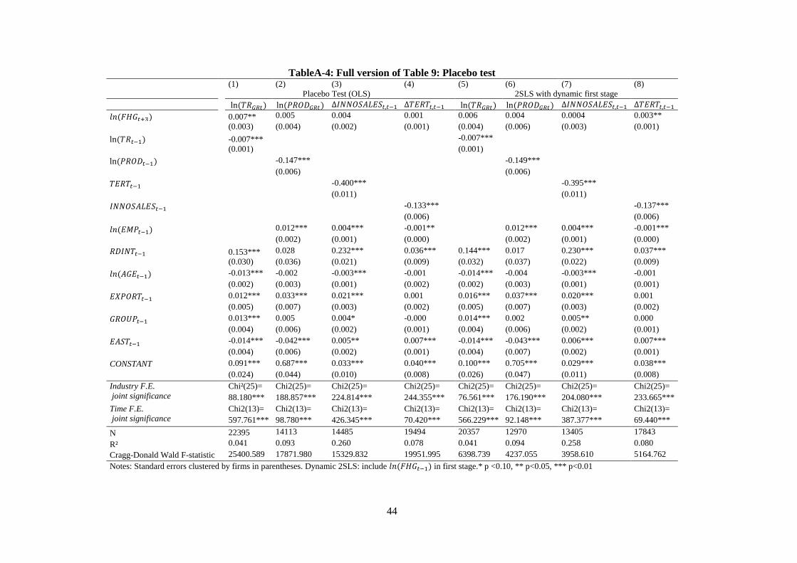
44
TableA-4: Full version of Table 9: Placebo test
(1) (2) (3) (4) (5) (6) (7) (8)
Placebo Test (OLS) 2SLS with dynamic first stage
ln (𝑇𝑅𝐺𝑅𝑡) ln (𝑃𝑅𝑂𝐷𝐺𝑅𝑡) Δ𝐼𝑁𝑁𝑂𝑆𝐴𝐿𝐸𝑆𝑡,𝑡−1 Δ𝑇𝐸𝑅𝑇𝑡,𝑡−1 ln (𝑇𝑅𝐺𝑅𝑡) ln (𝑃𝑅𝑂𝐷𝐺𝑅𝑡) Δ𝐼𝑁𝑁𝑂𝑆𝐴𝐿𝐸𝑆𝑡,𝑡−1 Δ𝑇𝐸𝑅𝑇𝑡,𝑡−1
𝑙𝑛(𝐹𝐻𝐺𝑡+3) 0.007** 0.005 0.004 0.001 0.006 0.004 0.0004 0.003**
(0.003) (0.004) (0.002) (0.001) (0.004) (0.006) (0.003) (0.001)
ln(𝑇𝑅𝑡−1) -0.007*** -0.007***
(0.001) (0.001)
ln (𝑃𝑅𝑂𝐷𝑡−1) -0.147*** -0.149***
(0.006) (0.006)
𝑇𝐸𝑅𝑇𝑡−1 -0.400*** -0.395***
(0.011) (0.011)
𝐼𝑁𝑁𝑂𝑆𝐴𝐿𝐸𝑆𝑡−1 -0.133*** -0.137***
(0.006) (0.006)
𝑙𝑛(𝐸𝑀𝑃𝑡−1) 0.012*** 0.004*** -0.001** 0.012*** 0.004*** -0.001***
(0.002) (0.001) (0.000) (0.002) (0.001) (0.000)
𝑅𝐷𝐼𝑁𝑇𝑡−1 0.153*** 0.028 0.232*** 0.036*** 0.144*** 0.017 0.230*** 0.037***
(0.030) (0.036) (0.021) (0.009) (0.032) (0.037) (0.022) (0.009)
𝑙𝑛(𝐴𝐺𝐸𝑡−1) -0.013*** -0.002 -0.003*** -0.001 -0.014*** -0.004 -0.003*** -0.001
(0.002) (0.003) (0.001) (0.002) (0.002) (0.003) (0.001) (0.001)
𝐸𝑋𝑃𝑂𝑅𝑇𝑡−1 0.012*** 0.033*** 0.021*** 0.001 0.016*** 0.037*** 0.020*** 0.001
(0.005) (0.007) (0.003) (0.002) (0.005) (0.007) (0.003) (0.002)
𝐺𝑅𝑂𝑈𝑃𝑡−1 0.013*** 0.005 0.004* -0.000 0.014*** 0.002 0.005** 0.000
(0.004) (0.006) (0.002) (0.001) (0.004) (0.006) (0.002) (0.001)
𝐸𝐴𝑆𝑇𝑡−1 -0.014*** -0.042*** 0.005** 0.007*** -0.014*** -0.043*** 0.006*** 0.007***
(0.004) (0.006) (0.002) (0.001) (0.004) (0.007) (0.002) (0.001)
CONSTANT 0.091*** 0.687*** 0.033*** 0.040*** 0.100*** 0.705*** 0.029*** 0.038***
(0.024) (0.044) (0.010) (0.008) (0.026) (0.047) (0.011) (0.008)
Industry F.E.
joint significance
Chi²(25)=
88.180***
Chi2(25)=
188.857***
Chi2(25)=
224.814***
Chi2(25)=
244.355***
Chi2(25)=
76.561***
Chi2(25)=
176.190***
Chi2(25)=
204.080***
Chi2(25)=
233.665***
Time F.E.
joint significance
Chi2(13)=
597.761***
Chi2(13)=
98.780***
Chi2(13)=
426.345***
Chi2(13)=
70.420***
Chi2(13)=
566.229***
Chi2(13)=
92.148***
Chi2(13)=
387.377***
Chi2(13)=
69.440***
N 22395 14113 14485 19494 20357 12970 13405 17843
R² 0.041 0.093 0.260 0.078 0.041 0.094 0.258 0.080
Cragg-Donald Wald F-statistic 25400.589 17871.980 15329.832 19951.995 6398.739 4237.055 3958.610 5164.762
Notes: Standard errors clustered by firms in parentheses. Dynamic 2SLS: include 𝑙𝑛(𝐹𝐻𝐺𝑡−1) in first stage.* p <0.10, ** p<0.05, *** p<0.01
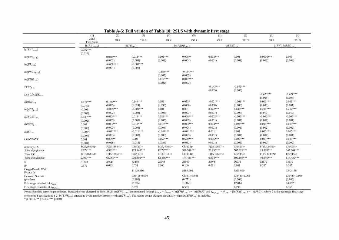
45
Table A-5: Full version of Table 10: 2SLS with dynamic first stage (1) (2) (3) (4) (5) (1) (2) (3) (4)
2SLS
First Stage OLS 2SLS OLS 2SLS OLS 2SLS OLS 2SLS
ln (𝐹𝐻𝐺𝑡−1) ln (𝑇𝑅𝐺𝑅𝑡) ln (𝑃𝑅𝑂𝐷𝐺𝑅𝑡) Δ𝑇𝐸𝑅𝑇𝑡,𝑡−1 Δ𝐼𝑁𝑁𝑂𝑆𝐴𝐿𝐸𝑆𝑡,𝑡−1
ln (𝐹𝐻𝐺𝑡−2) 0.752***
(0.014)
𝑙𝑛(𝐹𝐻𝐺𝑡−1) 0.010*** 0.013*** 0.008*** 0.008** 0.003*** 0.001 0.0006*** 0.003 (0.002) (0.003) (0.002) (0.004) (0.001) (0.001) (0.002) (0.002)
𝑙𝑛(𝑇𝑅𝑡−1) -0.008*** -0.008***
(0.001) (0.001)
𝑙𝑛(𝑃𝑅𝑂𝐷𝑡−1) -0.154*** -0.154***
(0.005) (0.005)
𝑙𝑛(𝐸𝑀𝑃𝑡−1) 0.012*** 0.012***
(0.002) (0.002)
𝑇𝐸𝑅𝑇𝑡−1 -0.143*** -0.142***
(0.005) (0.005)
𝐼𝑁𝑁𝑂𝑆𝐴𝐿𝐸𝑆𝑡−1 -0.425*** -0.424***
(0.008) (0.008)
𝑅𝐷𝐼𝑁𝑇𝑡−1 0.174*** 0.146*** 0.144*** 0.053* 0.053* -0.001*** -0.001*** 0.003*** 0.003*** (0.040) (0.025) (0.024) (0.030) (0.030) (0.000) (0.000) (0.000) (0.001)
𝑙𝑛(𝐴𝐺𝐸𝑡−1) -0.003 -0.009*** -0.009*** 0.001 0.001 0.042*** 0.043*** 0.210*** 0.212*** (0.003) (0.002) (0.002) (0.003) (0.003) (0.007) (0.007) (0.017) (0.017)
𝐸𝑋𝑃𝑂𝑅𝑇𝑡−1 0.030*** 0.013*** 0.013*** 0.028*** 0.028*** -0.002*** -0.002*** -0.002*** -0.002*** (0.002) (0.003) (0.003) (0.005) (0.005) (0.001) (0.001) (0.001) (0.001)
𝐺𝑅𝑂𝑈𝑃𝑡−1 0.007 0.013*** 0.013*** 0.013*** 0.013*** 0.004*** 0.004*** 0.019*** 0.019*** (0.005) (0.003) (0.003) (0.004) (0.004) (0.001) (0.001) (0.002) (0.002)
𝐸𝐴𝑆𝑇𝑡−1 -0.002* -0.011*** -0.011*** -0.041*** -0.041*** 0.001 0.001 0.005*** 0.005*** (0.004) (0.003) (0.003) (0.005) (0.005) (0.001) (0.001) (0.001) (0.001)
CONSTANT 0.001 0.059** 0.008 0.657*** 0.620*** 0.006*** 0.006*** 0.005*** 0.005*** (0.004) (0.028) (0.013) (0.034) (0.032) (0.001) (0.001) (0.002) (0.002)
Industry F.E.
joint significance
F(25,16436)=
6.979***
F(25,13864)=
4.992***
Chi²(25)=
123.948***
F(25, 9166)=
12.797***
Chi²(25)=
320.540***
F(25,12657)=
20.250***
Chi²(25)=
507.929***
F(25,12452)=
13.828***
Chi²(25)=
347.064***
Time F.E.
joint significance
F(15,16436)=
2.960***
F(15,13864)=
61.960***
Chi²(15)=
930.890***
F(14,9166)=
12.436***
Chi²(14)=
174.411***
F(15,12657)=
6.934***
Chi²(15)=
106.105***
F(15, 12452)=
40.946***
Chi²(15)=
614.439***
N 51878 43848 43848 23949 23949 36076 36076 33679 33679
R² 0.572 0.033 0.033 0.100 0.100 0.081 0.081 0.287 0.287
Cragg-Donald Wald
F-statistic 11129.816 5884.586 8355.850 7342.186
Hansen J Statistic
(p-value)
Chi²(1)=0.000
(0.986)
Chi²(1)=0.085
(0.771)
Chi²(1)=1.066
(0.302)
Chi²(1)=0.164
(0.686)
First stage t-statistic of 𝑧𝑒𝑚𝑝 21.224 16.163 17.814 14.852
First stage t-statistic of 𝑧𝑓ℎ𝑔𝑡−2 8.072 6.503 6.798 6.169
Notes: Standard errors in parentheses. Standard errors clustered by firm. 2SLS: 𝑙𝑛(𝐹𝐻𝐺𝑖,𝑡−1) instrumented through 𝑧𝑒𝑚𝑝 = ��𝑖,𝑡−1 ∗ [ln (𝐸𝑀𝑃𝑖,𝑡−1) − ln(𝐸𝑀𝑃) ] and 𝑧𝑓ℎ𝑔𝑡−2= ��𝑖,𝑡−1 ∗ [ln (𝐹ℎ𝐺𝑖,𝑡−2) − ln(𝐹ℎ𝐺) ], where �� is the estimated first-stage
error term. Specifications 1-2: 𝑙𝑛(𝐸𝑀𝑃𝑡−1) omitted to avoid multicollinearity with 𝑙𝑛(𝑇𝑅𝑡−1). The results do not change substantially when 𝑙𝑛(𝐸𝑀𝑃𝑡−1) is included.
* p <0.10, ** p<0.05, *** p<0.01