Do “Broken Windows” Matter? Identifying Dynamic

Spillovers in Criminal Behavior

Gregorio Caetano & Vikram Maheshri

⇤

May 9, 2013

Abstract

The “Broken Windows” theory of crime prescribes “zero-tolerance” law enforcementpolicies that disproportionately target light crimes with the understanding that thiswill lead to future reductions of more severe crimes. We provide evidence against theeffectiveness of such policies using a novel database from Dallas. Our identificationstrategy explores detailed geographic and temporal variation to isolate the causal be-havioral effect of prior crimes on future crimes and is robust to a variety of sources ofpotential endogeneity. We also estimate the effectiveness of alternative targeting poli-cies to discuss the efficiency of “Broken Windows” inspired policies. JEL Codes: K42 ,

R23.

1 Introduction

Economic models of crime are built upon the notion that would-be criminals consider thebenefits of committing crime, the probability of arrest and the potential costs of punishmentwhen making decisions (Becker (1968)). In a static model, individual- and neighborhood-level heterogeneity in both the expected costs and benefits of committing various crimesalong with agents’ beliefs regarding these costs and benefits imply an equilibrium in whichcrime levels vary across neighborhoods and by different types of crimes (Fender (1999)). If,however, the expected costs and benefits of crime are determined in part by the past historiesof criminal behavior in different neighborhoods, then crime must be understood as a socialand dynamic phenomenon.

⇤Departments of Economics, University of Rochester and University of Houston. We thank CarolinaCaetano, David Card, Aimee Chin, Scott Cunningham, Ernesto Dal Bo, Frederico Finan, Willa Friedman,Justin McCrary, Noam Yuchtman and various seminar and conference participants for valuable discussions.All errors are our own.

1

The leading theory that argues for the existence of intertemporal links in criminal be-havior is the “Broken Windows” (BW) theory of crime (Kelling and Coles (1998)).1 TheBW theory is developed around a social and dynamic mechanism by which the proliferationof less severe crimes (e.g., broken windows or graffiti) signals to potential criminals thatenforcement, and hence punishment, is lax in the area. This leads to future crimes of in-creasing frequency and severity, each one signaling further to future potential criminals thatenforcement is lax. Put differently, signals transmitted among potential criminals lead toherding behavior (Banerjee (1992); Bikhchandani et al. (1992)).2 Accordingly, BW carries astrong policy implication that addressing less severe crimes today can be an effective meansto reduce the future rates of more severe crimes indirectly (Kelling and Sousa (2001)). Withthis in mind, we refer to a BW law enforcement policy as one that disproportionally targetsless severe crimes. A number of US cities have implemented BW policies in the past twentyyears, notably among them New York City and Los Angeles, and such policies continue tobe influential.3 For instance the Chicago Police Department has recently subscribed to BWtheory to combat their current increase in violent crime.4

For such an important and currently relevant policy question, it is surprising that thistheory has undergone relatively little empirical validation. A few studies (Kelling and Sousa(2001), Funk and Kugler (2003) and Corman and Mocan (2005)) have attempted to analyzewhether targeting less severe crimes in the present has been effective in reducing more vio-lent crimes in the future, but as pointed out by Harcourt (1998) and Harcourt and Ludwig(2006)5 all of them are not able to claim causal estimates.6 We argue below that the inability

1James Q. Wilson is regarded as one of the originators of this theory (see Kelling, George L. and JamesQ. Wilson, “Broken Windows,” The Atlantic Monthly, March 1982.)

2Other dynamic models of crime focus on the relationships between criminal decisions and the labormarket (Davis (1988); Imai and Krishna (2004)), income inequality and crime (Fajnzlber et al. (2002)) andsocial networks and crime (Calvo-Armengol and Zenou (2004)). Glaeser et al. (1996) present a model ofcrime based on social interactions between criminals to explain geographic variation in crime rates.

3In a 2003 interview with the Academy of Achievement, former New York mayor Rudy Giuliani remarked,“I very much subscribe to the “Broken Windows” theory... The idea of it is that you had to pay attention tosmall things, otherwise they would get out of control and become much worse.”

4From the Chicago Tribune, 3/12/2013: “Chicago police Superintendent Garry McCarthy said Mondaythat he wanted to bring a “broken windows” strategy to Chicago that would allow officers to arrest thosewho ignore tickets for routine offenses like gambling and public urination.”

5 Harcourt and Ludwig (2006) take advantage of a random allocation of public housing under the “Movingto Opportunity” experiment in five US cities and find no effect of neighborhood misdemeanor crime levelson the propensity to commit violent crime among those who were assigned to that neighborhood, but itis difficult to attribute this finding to neighborhood misdemeanor crime levels rather than to unobservedcharacteristics of the neighborhood.

6There does seem to exist some indirect experimental evidence in favor of the mechanism underlying BWpolicies. Braga and Bond (2008) randomize police efforts to reduce social disorder in certain neighborhoods of

2

to uncover causal estimates is likely due to a lack of crime data available at detailed levelsof both geographic and temporal disaggregation. In addition, there has been no study toour knowledge that evaluates the trade-offs related to targeting less severe crimes versusalternative targeting strategies, so we know little about the relative efficiency of BW poli-cies. A complete economic analysis of BW policies must address the broader issue of theopportunity cost of these policies. Such an analysis requires researchers to not only measurethe effectiveness of policies that target less severe crimes but also the effectiveness of policiesthat target alternative types of crimes. Moreover, these measurements of policy effectivenessmust be considered in the context of the costs of targeting each type of crime and the socialbenefits of reducing each type of crime. This paper attempts to close some of these gapsin the literature. First, we provide causal estimates of the effect of reducing a particulartype of crime in the present on the levels of many different types of crime in the future.With these estimates of effectiveness, we can compute the full dynamic spillovers that areassociated with various crime reduction policies. Combined with external estimates of thesocial benefits of reducing various types of crimes (Miller et al. (1993); Heaton (2010)), weare able to provide a more complete analysis of whether policies that preferentially aim toreduce light crime, such as those prescribed by BW theory, should be implemented.

In order to motivate our empirical analysis, it is important to define precisely the in-tertemporal relationship that we seek to identify because crime in the past may cause futurecrimes of various types through a number of mechanisms. From the perspective of a lawenforcement policy maker, we argue that it is necessary to distinguish behavioral mechanismsfrom the overall intertemporal causal effect of crime, which also includes policy based mech-anisms. Behavioral mechanisms fully characterize the dynamic process of criminality andinclude social learning mechanisms in addition to individual learning mechanisms and anyother endogenous responses to prior crimes that are outside of the purview of law enforce-ment (e.g., formation of neighborhood watches by private residents).7 In contrast, policybased mechanisms include the future responses of law enforcement agencies to changes in

Lowell, Massachusetts and find that increased policing reduces citizen calls for service for more severe crimes,though measurement error in citizen reporting may be a source of concern in their study. In addition, Keizeret al. (2008) provide evidence from field experiments that is consistent with the behavioral mechanism atthe core of BW by showing that when individuals observe violations of social norms, they are more likelyto violate these norms themselves. It may be difficult, however, to interpret the external validity of thesehighly stylized, small-scale field experiments.

7Several models of social learning (Gul and Lundholm (1995); Gale (1996); Bikhchandani et al. (1998))have been developed from a rich theoretical literature on social interactions (Thibaut and Kelley (1959);Becker (1974); Manski (2000); Jackson and Watts (2002)), and they form the causal links explicitly discussedin the BW theory through which past crimes affect current and future crimes. However, past crimes mayaffect future crimes through non-social channels as well (e.g., learning by doing). As such, we conductour analysis from a broader perspective without focusing on disentangling these mechanisms suggested bycompeting theories.

3

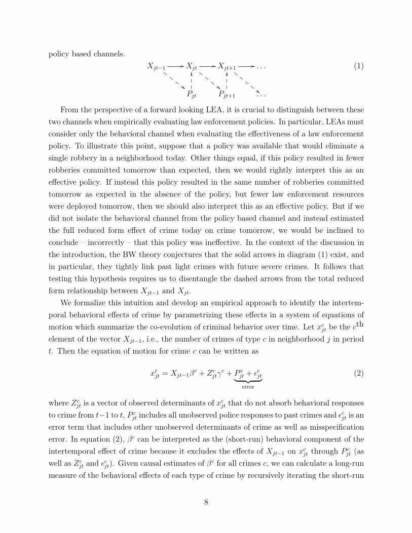
past crime levels. The main thrust of the BW theory is that in any period, a reduction in lesssevere crimes today will endogenously generate reductions in more severe crimes tomorroweven if future law enforcement activity is unchanged. Thus, in order to measure the effec-tiveness of a policy that targets light crime, it is imperative to identify the intertemporalcausal effects of crime independently of changes in future law enforcement policy. We musttherefore identify only those dynamic spillovers that arise from behavioral sources. Thisplays a particularly important role in the comparison of the effectiveness of alternative lawenforcement policies. For example, if a reduction of one robbery today tends to induce alarger change in the response of police than a unit reduction of a less severe crime, then notcontrolling for future police response will yield a biased comparison of these crime reductionpolicies.

Briefly, we conduct our analysis in two stages. In the first stage, we estimate causalequations of motion for each type of crime, which summarize the short run co-evolution ofall types of crimes over time. These equations describe the current levels of a given typeof crime as causal functions of the previous levels of each type of crime as well as otherdeterminants of crime. Importantly, our estimates of these causal criminal relationshipsonly include intertemporal behavioral effects. In the second stage, we use these estimates tosimulate the impulse responses of crime reduction, i.e., the long run effects of reductions inthe present level of a given crime on the future levels of each crime holding all else constant.8

We pay particular attention to the long run effects of crime reductions that would be typicalof BW law enforcement policies (reductions in light crimes).

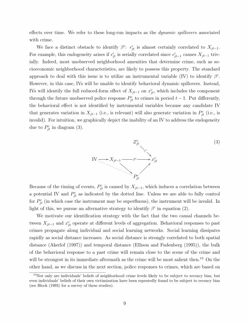
In identifying the causal, intertemporal (short run) behavioral effects in the first stage,we must address the fact that unobserved determinants of future crimes may be correlatedto previous crime levels (i.e., the usual endogeneity due to omitted variables). The standardmethod to deal with this issue – the use of instrumental variables – is unsuitable for our taskbecause it will necessarily identify the total reduced-form effect of previous crimes on futurecrime, which includes the policy based intertemporal effect of crimes.9

In light of these issues, we develop an identification strategy that leverages a novel,incident based dataset of crimes. Our identification strategy explores the fact that the

8This two stage procedure is necessary because it implicitly accounts for the fact that crime data maynot be observed in long run equilibrium but rather along some trajectory. Caetano and Maheshri (2012)discuss this topic in further detail.

9 Jacob et al. (2007) use city-wide weekly weather shocks as instruments and find a small negative within-crime intertemporal relationship. However, they focus only on within-crime effects at the city level and donot distinguish between behavioral and policy based intertemporal links between crimes, so their results areunrelated to BW policing.

4

behavioral effect of crime tends to be highly localized and tend to occur over short timespans, while other confounding effects, including policy responses to prior crimes, do not.Thus, we can exploit the high geographic detail and the high frequency of our data to isolatethe behavioral effect from the other effects. Our identification strategy has a firm theoreticaland institutional basis. As discussed in Akerlof (1997) and Ellison and Fudenberg (1995),social learning depends crucially upon the “social distance” between agents which is stronglyrelated to both physical and temporal distance. Moreover, other endogenous responsesto crime which are deemed behavioral are clearly local and at high frequency, as in thecase of individual learning mechanisms (e.g., learning-by-doing, Arrow (1962)), individualspecialization in criminal activity (Kempf (1987)), individual incapacitation (Levitt (1998))and other endogenous neighborhood responses to crime (Taylor (1996)). However, othersystematic determinants of crime such as neighborhood wealth levels (Flango and Sherbenou(1976)) and family structure (Sampson (1985)) vary more slowly than crime itself, andinstitutional knowledge allows us to conclude that the immediate policy response to crimeby law enforcement is based on larger administrative boundaries that encompass multiplesocial and individual learning networks. Thus, by focusing on the relationship between priorcrimes and current crimes within smaller neighborhoods and at shorter time scales, we canestimate intertemporal behavioral effects of crime that are plausibly independent of policyresponses or other confounding effects. The richness of our data set also allows us to provideempirical support for these theoretical and institutional arguments.

We supplement this identification strategy by conducting several robustness checks thataddress a variety of standard empirical issues often encountered with spatial panel datasetsincluding omitted variables, temporal and geographic misaggregation, serial correlation, spa-tial autocorrelation, and other forms of measurement error. As a final, novel robustnesscheck, we directly test whether our estimates are unbiased using a formal, statistical test ofexogeneity inspired by Caetano (2012) that is based on continuity conditions. We argue thatwith this test we are able in principle to detect endogeneity from a number of sources, in-cluding omitted variables, measurement error and unobserved future police actions. Indeed,in practice we detect endogeneity in specifications of the type that have been previouslyestimated in this literature, yet we do not detect endogeneity in our preferred specifications,which provides further validation of our identification strategy.

We conduct our analysis using a unique, comprehensive database that contains everypolice report filed with the Dallas Police Department from 2000-2007. In total, this databasecontains nearly 2 million unique police reports, including reported light crimes, such asbroken windows and graffiti, which are not observed in most criminal data sets and playa crucial role in assessing BW policies. Each police report narrowly classifies the crime

5

committed and contains detailed information regarding the precise location and time of thealleged crime.10 In addition, each police report contains information regarding the speedand quality of the police response to the report, which is also rarely observed. We use thisdatabase to construct a panel data set containing the weekly levels of six types of crimes(rape, robbery, burglary, motor vehicle theft, assault and light crime) in 32 neighborhoodsthat span the city of Dallas.

Although we find that a reduction of one light crime leads to an additional cumulativefuture reduction of roughly 0.1 light crimes, this reduction is not found to generate statis-tically or economically significant reductions in the future levels of more severe crimes. Weinterpret our finding that law enforcement actions that target light crimes are ineffective inreducing more severe crimes in the future as casting considerable doubt on the claim that thedramatic reduction in the crime rate (especially the violent crime rate) in US urban areasover the past fifteen years is due to the adoption of BW or zero-tolerance law enforcementpolicies.11 In sum, our findings suggest that law enforcement agencies aiming to reduceviolent crimes should pursue policies that are tailored to combat those crimes.

We acknowledge that even if a law enforcement action that targets light crime is ineffectiveat reducing future violent crime rates, it may still be preferred to other policies. To evaluatethis claim, we estimate the effectiveness of alternative targeting practices. We find that areduction of one robbery leads to an additional cumulative future reduction of roughly 0.1robberies, a reduction of one auto theft leads to an additional cumulative future reductionof 0.2 auto thefts, and a reduction of one burglary leads to an additional cumulative futurereduction of 0.4 burglaries. Although we find that unit reductions in assaults lead to futurereductions of nearly 0.005 rapes and 0.025 robberies, we find no statistically significantevidence of other dynamic spillovers across crimes of increasing severity. We do find thatunit reductions of robbery, auto theft and assaults generate spillover reductions of 0.18, 0.10and 0.05 light crimes respectively. These across-crime spillovers in the direction of decreasing

severity are of the same order of magnitude as the within-crime spillovers associated withlight crime, suggesting that actions that target more severe crimes will generate spilloverbenefits that strictly dominate the spillover benefits of actions that target light crimes. Thisstands in stark contrast to the policy prescriptions of BW theory.

To complete our analysis, we make the first attempt to evaluate the long run efficiency10The precise location and time of reported crimes are rarely observed in the same dataset, at least in

large, incident based criminal data sets that are relevant for this analysis such as the National Incident BasedReporting System (NIBRS).

11Levitt (2004) describes efforts by the media to attribute falling crime rates in New York City to innovativelaw enforcement policies, including “broken windows” style policies, but he argues that this conclusion ispremature given other confounding changes that occurred in New York City at the same time or even beforea “broken windows” policy was implemented. Our finding is consistent with this view.

6

of BW policies with a back of the envelope welfare calculation using external estimates ofthe social benefits of crime reduction from Heaton (2010) and Miller et al. (1993). We findthat a BW policy is advisable only if the marginal cost of reducing a light crime is less than25 (7) times the marginal cost of reducing a robbery (burglary).

The remainder of the paper is organized as follows. In section 2, we describe our strategyto identify intertemporal behavioral relationships between neighborhood crimes. In section 3,we describe our data set and discuss the plausibility of our identification strategy. In section4, we present estimates of the short run intertemporal effects of crime, and in section 5 weshow that those estimates withstand a variety of robustness checks. In particular, we derivea formal test of the exogeneity assumption underlying our identification strategy and use itto argue that our estimates of the intertemporal behavioral relationships between crimes areindeed unbiased.12 In section 6 we calculate long run dynamic spillovers in criminal behaviorby simulation, and we use these results to perform a back of the envelope cost-benefit analysisof various alternative law enforcement policies. We conclude in section 7.

2 Empirical Approach

Law enforcement agencies (LEAs) seek to choose and implement policies that generate thegreatest net benefit in terms of crime reduction. Forward looking LEAs must explicitlyconsider the long run benefits and costs of law enforcement policies, hence it is useful forthem to know the effects of past crimes on current and future crimes. Past crime affectscurrent (and future) crime through two channels: directly through behavioral changes, andindirectly through future policy responses. Behavioral channels include any endogenousintertemporal responses to prior crimes. For example, social learning by criminals (Ellisonand Fudenberg (1995)), learning-by-doing (Arrow (1962)), specialization in criminal activity(Kempf (1987)), incapacitation (Levitt (1998)), and neighborhood responses to crime (Taylor(1996), Bronars and Lott Jr (1998)) are all classified as behavioral channels. On the otherhand, policy based channels include any current police responses to prior crimes that affectcurrent crime levels. For example, a police crackdown (Sherman and Weisburd (1995))and a change in the distribution of police resources due to an increase in the number ofcrimes (Weisburd and Eck (2004)) are classified as policy based. We depict these two causalchannels in diagram (1). For a given neighborhood j, X

jt

is a vector containing the levels ofC types of crimes, and P

jt

represents the law enforcement policy implemented in period t.The solid arrows correspond to behavioral channels, while the dashed arrows correspond to

12 We provide theoretical and empirical support for the implementation of this test in appendix A.1.

7

policy based channels.X

jt�1//

""

Xjt

//

""

Xjt+1

//

""

. . .

Pjt

OO

Pjt+1

OO

. . .

(1)

From the perspective of a forward looking LEA, it is crucial to distinguish between thesetwo channels when empirically evaluating law enforcement policies. In particular, LEAs mustconsider only the behavioral channel when evaluating the effectiveness of a law enforcementpolicy. To illustrate this point, suppose that a policy was available that would eliminate asingle robbery in a neighborhood today. Other things equal, if this policy resulted in fewerrobberies committed tomorrow than expected, then we would rightly interpret this as aneffective policy. If instead this policy resulted in the same number of robberies committedtomorrow as expected in the absence of the policy, but fewer law enforcement resourceswere deployed tomorrow, then we should also interpret this as an effective policy. But if wedid not isolate the behavioral channel from the policy based channel and instead estimatedthe full reduced form effect of crime today on crime tomorrow, we would be inclined toconclude – incorrectly – that this policy was ineffective. In the context of the discussion inthe introduction, the BW theory conjectures that the solid arrows in diagram (1) exist, andin particular, they tightly link past light crimes with future severe crimes. It follows thattesting this hypothesis requires us to disentangle the dashed arrows from the total reducedform relationship between X

jt�1 and Xjt

.We formalize this intuition and develop an empirical approach to identify the intertem-

poral behavioral effects of crime by parametrizing these effects in a system of equations ofmotion which summarize the co-evolution of criminal behavior over time. Let xc

jt

be the cth

element of the vector Xjt�1, i.e., the number of crimes of type c in neighborhood j in period

t. Then the equation of motion for crime c can be written as

xc

jt

= Xjt�1�

c + Zc

jt

�c + P c

jt

+ ✏cjt| {z }

error

(2)

where Zc

jt

is a vector of observed determinants of xc

jt

that do not absorb behavioral responsesto crime from t�1 to t, P c

jt

includes all unobserved police responses to past crimes and ✏cjt

is anerror term that includes other unobserved determinants of crime as well as misspecificationerror. In equation (2), �c can be interpreted as the (short-run) behavioral component of theintertemporal effect of crime because it excludes the effects of X

jt�1 on xc

jt

through P c

jt

(aswell as Zc

jt

and ✏cjt

). Given causal estimates of �c for all crimes c, we can calculate a long-runmeasure of the behavioral effects of each type of crime by recursively iterating the short-run

8

effects over time. We refer to these long-run impacts as the dynamic spillovers associatedwith crime.

We face a distinct obstacle to identify �c: ✏cjt

is almost certainly correlated to Xjt�1.

For example, this endogeneity arises if ✏cjt

is serially correlated since ✏cjt�1 causes X

jt�1 triv-ially. Indeed, most unobserved neighborhood amenities that determine crime, such as so-cioeconomic neighborhood characteristics, are likely to possess this property. The standardapproach to deal with this issue is to utilize an instrumental variable (IV) to identify �c.However, in this case, IVs will be unable to identify behavioral dynamic spillovers. Instead,IVs will identify the full reduced-form effect of X

jt�1 on xc

jt

, which includes the componentthrough the future unobserved police response P c

jt

to crimes in period t� 1. Put differently,the behavioral effect is not identified by instrumental variables because any candidate IVthat generates variation in X

jt�1 (i.e., is relevant) will also generate variation in P c

jt

(i.e., isinvalid). For intuition, we graphically depict the inability of an IV to address the endogeneitydue to P c

jt

in diagram (3).

Zc

jt

�

c

IV // X

jt�1 �

c //

""

xc

jt

P c

jt

>>

(3)

Because of the timing of events, P c

jt

is caused by Xjt�1, which induces a correlation between

a potential IV and P c

jt

as indicated by the dotted line. Unless we are able to fully controlfor P c

jt

(in which case the instrument may be superfluous), the instrument will be invalid. Inlight of this, we pursue an alternative strategy to identify �c in equation (2).

We motivate our identification strategy with the fact that the two causal channels be-tween X

jt�1 and xc

jt

operate at different levels of aggregation. Behavioral responses to pastcrimes propagate along individual and social learning networks. Social learning dissipatesrapidly as social distance increases. As social distance is strongly correlated to both spatialdistance (Akerlof (1997)) and temporal distance (Ellison and Fudenberg (1995)), the bulkof the behavioral response to a past crime will remain close to the scene of the crime andwill be strongest in its immediate aftermath as the crime will be most salient then.13 On theother hand, as we discuss in the next section, police responses to crimes, which are based on

13Not only are individuals’ beliefs of neighborhood crime levels likely to be subject to recency bias, buteven individuals’ beliefs of their own victimization have been repeatedly found to be subject to recency bias(see Block (1993) for a survey of these studies).

9

administrative protocols of LEAs, are likely to be consistent within administrative regionsthat encompass multiple individual and social learning networks. Moreover, adjustments ofthe allocation of LEA resources within administrative regions is likely to occur at a slowerpace than behavioral responses to past crimes. In addition, other confounding causes ofcurrent crimes (✏c

jt

) also operate at more aggregated levels. For instance, the demographiccomposition of a neighborhood, which has been found to affect crime rates (Sampson (1985)),tends to change relatively slow over time. The same is true of judicial institutions includ-ing municipal arrest policies, criminal law, and incarceration policies. These differences inaggregation indicate an identification strategy that explores the geographic and temporaldetail of the panel data to construct fixed effects that absorb all confounding factors, includ-ing unobserved police responses, without absorbing any of the treatment effect we want tomeasure.

Formally, let a city be composed of neighborhoods indexed by j, which are further groupedinto administrative regions indexed by J . The shorter time periods t (e.g., weeks) at whichcrime levels are sampled can be further grouped into longer time periods T (e.g., years).14

We can decompose the sources of error in equation (2) into three pieces:

P c

jt

+ ✏cjt

= �c

Jt

+ �c

jT

+ ⌘cJTjt

(4)

where �c

Jt

is the average high frequency varying error in an administrative region, �c

jT

is theaverage low frequency varying error in a neighborhood, and ⌘cJT

jt

is the remaining error thatadditionally depends on the levels of aggregation of J and T . For the reasons describedabove, police responses are not likely to vary systematically within administrative regions ata given point in time. It follows that fixed effects at the crime type, administrative region andtime level (�c

Jt

) will absorb the future police response P c

jt

(along with all other confoundingcauses of crime that do not vary by administrative region). Similarly, fixed effects at thecrime type, neighborhood and longer time period level (�c

jT

) will absorb any neighborhoodspecific confounding factors ✏c

jt

that vary at the lower frequency T . Thus, the intertemporalbehavioral effect �c is identified under the following exogeneity assumption.

Assumption 1. E[⌘cJTjt

|Xc

jt�1,�c

Jt

,�c

jT

] = 0

Intuitively, there is an implicit trade-off in our choices of J and T (and j and t byextension). Assumption 1 is more likely to be valid for smaller choices of J and T because⌘cJTjt

will tend to be smaller (in absolute value) by construction. However choosing very

14Without loss of generality, we assume that neighborhoods are uniquely assigned to an administrativeregion (j 2 J implies j /2 J 0 for all J 0 6= J) and that longer time periods are evenly divisible by the shortertime periods (t 2 T implies t /2 T 0 for all T 0 6= T ).

10

small levels of J and T may result in some of the intertemporal behavioral effects beingabsorbed by the fixed effects, adversely impacting our interpretation of �r. It follows thatour choices of J and T should absorb as much of the confounding factors (P c

jt

and ✏cjt

) aspossible without absorbing any of the intertemporal behavioral effect. More formally, let J

and T be the minimal levels of J and T for which no component of the behavioral effectis absorbed by the fixed effects �c

Jt

and �c

jT

, and let J and T be the maximum levels of Jand T for which all confounding factors are absorbed by the fixed effects �c

Jt

and �c

jT

. Thenappropriate choices of J and T should satisfy the inequalities J J J and T T T .Before further discussing the theoretical, institutional, and empirical reasons why our choicesof J and T are likely to satisfy these conditions15, we first describe our data set.

3 Data and Preliminaries

3.1 Sample

We assemble a database encompassing every police report filed with the Dallas Police De-partment (DPD) from January 1, 2000 to September 31, 2007.16 According to the FBI,Dallas held the dubious distinction of having the highest crime rate of all US metropolitanareas with at least one million persons during the sample period.17 Although Dallas didnot explicitly adopt BW policing in this period, we can still analyze the dynamics of crimi-nal behavior using this data since we estimate these behavioral effects independently of lawenforcement policy.18 This database is uniquely suited to evaluate the effectiveness of BWpolicies because it includes a comprehensive catalog of all light crimes of various types thatwere reported.

Every report in our database lists the exact location (address or city block) of the crimeand is given a five digit Uniform Crime Reporting (UCR) classification by the respondingofficer.19 A full description of the complainant who called in the report is also provided, withthe exception of anonymous reports. Private companies and public officials/offices may belisted as complainants. Every report also lists a series of times from which we can deducethe entire sequence of crime, neighborhood response and police response. Specifically, we

15In particular, we argue below why J < J and T < T so that this identification strategy is feasible.16A small number of police reports – sexual offenses involving minors and violent crimes for which the

complainant (not necessarily the victim) is a minor – are omitted from our data set for legal reasons.17“New York Remains Safest Big City in US,” September 19, 2006, The Associated Press.

18The coefficients �c are inherent to the dynamic behavioral process of crime, which is, by definition, thesame irrespective of the policy.

19If a particular complaint consists of multiple crimes (e.g., criminal trespass leading to burglary), thenthe report is classified only under the most severe crime (burglary) per UCR hierarchy rules developed bythe FBI.

11

observe the time (or estimate of the time) that the crime was committed, the time at whichthe police were notified and dispatched, the time at which the police arrived at the scene ofthe crime, and the time at which the police departed the scene of the crime. This allows usto construct observable police response measures that vary geographically, temporally andby crime type and are correlated to the unobservables P c

jt

, which are valuable for showingthat our estimates of �c do not include (observable or unobservable) policy responses by lawenforcement.

We perform our analysis on six crimes: rape, robbery, burglary, motor vehicle theft,assault and light crime. Because of potential misclassification, we define assault as bothaggravated and simple assault (Zimring (1998)). We classify criminal mischief, drunk anddisorderly conduct, vice (minor drug offenses and prostitution), fence (trade in stolen goods)and found property (almost exclusively cars and weapons) as light crimes.20 Together, thesesix crimes comprise 55% of all police reports to the DPD during the sample period.21

We select this set of crimes for four reasons. First, this set of crimes includes both violentcrimes and property crimes of varying levels of severity, which allows us to test for dynamicspillover effects of lighter crimes to more severe crimes. Second, these crimes are likely tosignal criminals’ actual beliefs of the strength of enforcement to potential criminals, whichforms the basis of the social learning mechanism suggested by BW theory. In contrast, crimessuch as embezzlement and gambling are less publicly observable. Third, these crimes occurrelatively more frequently than other publicly observable crimes such as homicide and arson.And fourth, these crimes are relatively accurately reported in comparison with crimes suchas larceny and fraud.22

We provide summary statistics for these reported crimes in table 1. Not surprisingly, lightcrime is the most prevalent crime reported, followed by assault, burglary, auto theft, robberyand rape. Police respond to crimes in approximately 80 minutes on average, although theyrespond to reports of rape roughly an hour slower and to reports of motor vehicle theftroughly half an hour faster. On average, police spend less than half an hour at the sceneof a motor vehicle theft, but they spend up to an hour at the scenes of robberies and light

20As robustness checks, we replicated our full analysis defining only criminal mischief and found propertyas light crime, or alternatively defining criminal mischief only as light crime. In all three cases, we obtainedsimilar results.

21Roughly 25% of police reports in the database do not directly correspond to criminal acts per se (i.e.,they declare lost property, report missing persons, report the failure of motorists to leave identification afterauto damages, etc.) so the six crimes that we consider comprise a much larger majority of total crime inDallas during the sample period.

22The accuracy of reported rape statistics is admittedly poor (Mosher et al. (2010)). As an added ro-bustness check, we replicated our full analysis excluding rapes and obtained similar results. To the extentthat the propensity to misreport rape varies discontinuously at xc0

jt�1 = 0 for some c0, the test of exogeneitydescribed in section 5.3 will also detect endogeneity stemming from mismeasurement in rape levels.

12

crimes and over an hour at the scenes of reported rapes. All types of crimes occur slightlymore frequently on weekends than weekdays with the exception of burglaries, which happenless frequently on weekends than weekdays. Just over half of robberies, light crimes andmotor vehicle thefts occur at night, and as expected, a majority of these crimes take placeoutdoors. On the other hand, burglaries and assaults tend to occur during the daytime andindoors. Rapes tend to occur at night and indoors. Private businesses report approximateone fifth of robberies and light crimes and one third of burglaries, but they report very fewmotor vehicle thefts and no rapes or assaults.

3.2 Choosing J and T 23

Although we observe each crime individually, the relevant variables in our model are levels ofcrime in pre-defined neighborhoods and time periods. As such, we must geographically andtemporally aggregate our data in a careful manner that satisfies our identifying assumptionand preserves sufficient intertemporal and cross-sectional variation in crime levels.

During our sample period, DPD was geographically organized into six divisions sub-divided into 32 sectors, which were further subdivided into police beats.24 In the DPDhierarchy, division deputy chiefs are given a relatively high degree of autonomy in devisingrapid responses to crimes.25 For this reason, we choose J to be the division level. Policebeats range from roughly 0.5 to two square miles in area, and each sector contains five toseven beats. Ideally, we would like to define our panel at the largest geographic level thatcan maintain assumption 1 in order to internalize the information spillovers from observedcrime levels in nearby areas. This ensures that our estimate of �c contains as much of theintertemporal behavioral effect of crime as possible. Accordingly, we define neighborhoodsour panel at the j = sector level.

Because social learning may occur at high frequency, we would like to define our panelat the shortest temporal level for which we can still construct plausible crime rates. Wechoose t = week, which preserves substantial heterogeneity in neighborhood crime rates overtime and provides a long time series (402 periods). Because neighborhood level confounding

23Empirical justification for our choices of J and T is provided following our main results.24In October 2007, DPD added a seventh division to their classification and made slight modifications to

some beat and sector boundaries. We end our sample in September 2007 to ensure that the administrativeboundaries in our data set are geographically consistent over the entire sample period.

25As depicted in the DPD Organizational Chart (http://www.dallaspolice.net/content/11/66/uploads/DPDOrgChart-4-11-13.pdf) the Patrol Bureau of the DPD, which is in charge of devising short run responses to crimes, isdecentralized at the division level and led by Deputy Chiefs, who are starred commanders for each division.This decentralization is discussed in detail in the publicly available Dallas Police Department Management

and Efficiency Study, prepared by a third party, Berkshire Advisers, Inc., for the DPD in September 2004.

13

determinants of crime are likely to vary slowly, we choose T to be yearly. We make this choicefor two reasons. First, this choice embeds much of the previous literature on estimatingintertemporal effects of crime that relies on annually varying controls (e.g., Funk and Kugler(2003); Corman and Mocan (2005)). Second, this choice allows us to estimate medium-runintertemporal behavioral effects of crime that propagate at an intermediate frequency (e.g.,monthly) and may dissipate nonlinearly.

4 Estimation Results

We estimate �1, . . . , �C from the following system of equations

x1jt

= Xjt�1�

1 + Z1jt

�1 +D1�1 + u1it

... (5)

xC

jt

= Xjt�1�

C + ZC

jt

�C +DC�C + uC

it

,

which represent the equations of motion of all crimes (C = 6). Given the large numberof estimated parameters, we report only the subset of the results that are most directlyrelevant to evaluate the effectiveness of BW policies in the body of the paper. The completeset of estimates of �c for all types of crime are reported in the online appendix. Coefficientestimates of the effects of light crime on future levels of all other crimes are presentedfor various specifications in table 2. In each specification, the system of equations (5) isestimated efficiently by Seemingly Unrelated Regression (Zellner (1962)). Given that theprimary source of bias is likely to be omitted determinants of crime that are positivelyserially correlated (e.g., neighborhood amenities), we would expect our naive estimates of �c

to be biased upward in specifications with insufficient controls.In specification 1, we do not include any control variables. We find that an additional

light crime is associated with approximately half of an additional reported light crime inthe following week. Moreover, with this specification we find that an additional light crimehas an intertemporal effect on more severe crimes such as assault, auto theft and burglary,which suggests that BW policies are effective in reducing more severe crimes. All coefficientsare precisely estimated, and we are able to explain 81% of the variation in reported weeklyneighborhood crime levels with this specification.

In specification 2, we add year-crime type fixed effects as control variables. These vari-ables absorb any annually varying determinants of each type of crime that are common toall neighborhoods in Dallas. Previous attempts to identify intertemporal relationships be-tween crimes (Funk and Kugler (2003)) and between crime and policing (Corman and Mocan

14

(2005)) are based on specifications similar to this, as they utilize only low-frequency controlvariables with low geographic detail (such as city-wide or national annual unemploymentrates) which are absorbed by the fixed effects in specification 2. The coefficient estimatesof this specification are roughly similar to our estimates from specification 1. Indeed theincrease in R2 of 0.002 from specifications 1 to 2 indicate that these control variables explainlittle additional variation in weekly neighborhood crime rates.

In specification 3, we add sector (j)-crime type fixed effects and week (t)-crime typefixed effects as control variables. These variables absorb any omitted neighborhood specificdeterminants of each crime and any omitted city-wide week specific determinants of eachcrime respectively. Overall the coefficient estimates are precisely estimated but decreasein magnitude relative to specifications 1 and 2, which confirms our conjecture that theseomitted variables are positively correlated with criminal activity. This finding casts doubton the results of earlier empirical studies of the effectiveness of BW policy and highlights theimportance of using high frequency and geographically detailed data to identify intertemporalbehavioral effects of crime. Nevertheless, reducing light crime is still found to be effective inreducing future levels of more severe crimes in this specification. With the inclusion of thesefixed effects, we are able to explain 85% of the variation in reported weekly neighborhoodcrime levels.

In specification 4, we enrich the set of control variables by disaggregating the fixed effectsby sector (j)-year (T )-crime type and division (J)-week (t)-crime type. As discussed above,these fixed effects are uniquely suited to control for endogeneity from unobserved policeresponses to crime as well as from other confounding factors. The first set of fixed effectsabsorbs all omitted neighborhood specific determinants of each crime that vary on an annualbasis (e.g., demographic characteristics of the neighborhood).26 The second set of fixed effectsabsorbs all time varying determinants of each crime that vary across the six police divisionsof Dallas, which importantly includes high frequency division level responses to prior crimes.In short, the only potential omitted variable that could bias our estimates would have to beboth sector-specific and vary across weeks within a calendar year or both week-specific andvary across sectors within a division. As in the previous specifications, all coefficients areprecisely estimated. Parameter estimates in this specification are substantially smaller inmagnitude than in the previous specifications. Indeed, previous light crimes are still foundto cause future light crimes, but this effect is only about a third as large as in specification3. More importantly, in this specification, we find no statistically or economically significant

26 Sector specific unobservable amenities that are changing over time due to gentrification will be partiallyabsorbed by these fixed effects to the extent that they vary across years in the sample.

15

intertemporal effect of light crime on more severe crimes of any type, so we find no evidencethat targeting light crime is an effective means of reducing more severe crimes in the future.27

This suggests that the estimates in specification 3 are biased. With these fixed effects, weare able to explain 87% of the variation in reported weekly neighborhood crime levels.

In specifications 5 and 6, we show that our estimates of �c from specification 4 arerobust to a variety of different sources of potential endogeneity. In specification 5, we enrichour set of control variables by including the shares of each type of crime reported to havebeen committed in the daytime and on the weekend in the previous week and the shares ofeach type of crime reported to have been committed outdoors in the previous week.28 Thisallows us to explore if either our temporal or spatial aggregation of observations introducesendogeneity into our specification. If crimes committed during the daytime or during theweekend (outdoor) generate different intertemporal effects than crimes committed at nighttime or during the weekday (indoor), perhaps because they are more salient to a potentialcriminal, then specification 4 would be temporally (spatially) misspecified, which might biasour parameter estimates. That we find almost no change in either the coefficient estimatesor the R2 between specifications 4 and 5 suggests that our choices of j and t do not bias theresults.

In specification 6 we expand the set of control variables from specification 5 by adding,for each type of crime, the average time that the police take to arrive at the crime scenein the current week, and the average duration that police remain at the crime scene in thecurrent week.29 We include these variables to attempt to proxy for the level of attentionthat the police pay each type of crime in each particular neighborhood in the current week,i.e., the police response to prior crimes. The inclusion of these variables have no discernibleeffect on the estimates of �c, nor do they explain any additional variation in reported weeklyneighborhood crime levels. Indeed, we a test of the hypothesis that all 72 police responseand police duration coefficients are equal to zero yields a p-value of .66. We interpret this asstrong evidence that the fixed effects successfully absorb unobserved determinants of policeresponsiveness.

27Gladwell (2000) has popularized the notion that BWT implies the existence of a “tipping point” level oflight crime beyond which the levels of light crime and more severe crimes are on an ever increasing trajectory.Our findings that the eigenvalues of the estimated � matrix (which includes �c for all equations of motion)are much smaller than one are inconsistent with this view (see, e.g., Lade and Gross (2012)).

28Given the system of 6 equations of motion, each with 6 main explanatory variables, we effectively add36 control variables for daytime crimes, 36 control variables for weekend crimes and 36 control variables foroutdoor crimes.

29As in specification 5, we effectively add 36 average police response and 36 average police durationvariables as controls in specification 6.

16

5 Additional Robustness Checks

In table 2, we present evidence that the estimates of specifications 1 through 3 are biased, butwe were unable to find evidence that the estimates of specifications 4 through 6 are biased.In this section, we leverage our detailed dataset to subject these specifications to strongerrobustness checks that in part provide further empirical evidence in favor of our choices ofJ , T , j and t. Because reported crime levels have been found to suffer from non-classicalmeasurement error (e.g., Skogan (1974, 1975, 1977)) we also conduct robustness checks thatare particularly sensitive to this issue and test for spatially autocorrelated errors, seriallycorrelated errors, and general errors due to misreporting of crime. Our results in this sectionare strongly consistent with the results presented in table 2 in the sense that specifications 1through 3 repeatedly fail these additional robustness checks whereas specifications 4 through6 do not fail any of the tests.

5.1 Spatial Autocorrelation

Determinants of crime are potentially spatially autocorrelated across neighboring regions(e.g., Morenoff and Sampson (1997)) for two reasons. First, the levels of unobserved deter-minants of crime in a particular neighborhood may be correlated with the levels of thosedeterminants in nearby neighborhoods, generating positive spatial autocorrelation. Second,crime in one neighborhood may displace crime from nearby neighborhoods, generating neg-ative spatial autocorrelation (Cornish and Clarke (1987)). If determinants of crime arespatially autocorrelated, then our estimates �c may be biased due to endogeneity, and theirstandard errors may also be biased, affecting inference.

In specifications 4-6, we attempted to address this form of endogeneity by adding fixedeffects at the division-week-crime type level (�c

Jt

) to absorb any unobservable determinantof crime that is common across neighboring sectors. If the endogeneity problem is addressedby the control variables in our preferred specifications, then we would expect that the errorsin such specifications would be spatially uncorrelated. Accordingly, we follow the suggestionof Dube et al. (2010) and re-estimate the system of equations and cluster the standarderrors at a larger geographic level than our panel (by division-year-crime type as opposedto by sector-year-crime type). By doing so, we allow ⌘cJT

jt

to be correlated with ⌘cJTkt

, wherej and k are sectors within the same division of Dallas. In table 3, we reproduce all ofthe standard errors from the specifications presented in table 2 in bold. Directly belowthese standard errors in normal font, we present all of the standard errors clustered at thedivision-year-crime type. Two findings are immediate. First, the original standard errorsclustered by sector-year-crime type differ substantially from the standard errors clustered

17

by division-year-crime type in specifications 1-3.30 Second, the standard errors clusteredby division-year-crime type are nearly identical to the standard errors clustered by sector-year-crime type in specifications 4-6; that is, in these specifications, any previously estimatedstatistically significant intertemporal effect remains statistically significant under the broaderclustering, and vice versa. These findings taken together suggest that the additional controlvariables in our preferred specifications effectively absorb potential spatial autocorrelationin the errors, while the control variables in specifications 1-3 do not.

We provide further evidence against spatial autocorrelation by re-estimating the systemof equations with additional controls for crime in nearby neighborhoods. In particular, weinclude X̃

jt�1 as control variables, where X̃jt�1 contains the crime levels of the closest sector

to sector j that is within the same division. If the intertemporal behavioral effect spillsover to other neighborhoods (sectors) within the same division, then we would expect thecoefficients of X̃

jt�1 to be different from zero. However, an F-test of the hypothesis that all36 coefficients of X̃

jt�1 equal zero yields a p-value of 0.24, which constitutes strong evidenceagainst spatial autocorrelation and in favor of our claim that our choice of j = sectorfully incorporates all intertemporal behavioral effects. In addition, our estimates of �c areunchanged from before.

The results of specification 6 of table 2 and these results taken together suggest that theminimal level of J for which no component of the behavioral effect is absorbed (J) is weaklysmaller than a sector, and the maximum level of J for which all confounding factors areabsorbed (J) is weakly larger than a division. Hence, our choice of J = division is consistentwith the identifying assumption (i.e., J < J J).

5.2 Serial Correlation

Determinants of crime may also be serially correlated (Fajnzylber et al. (2002)), which hastwo implications for our empirical analysis. First, serially correlated errors may be a source ofendogeneity, hence our estimates of �c might be biased. Second, positively serially correlatederrors may make inference misleading, as standard errors may be too small. In specifications4-6, we attempted to address this form of endogeneity by adding sector-year-crime type fixedeffects (�c

jT

) in order to absorb neighborhood specific unobservables that are common acrossweeks within year.

As suggested by Angrist and Pischke (2009), we provide a further robustness check byre-clustering our standard errors at the sector-year-crime type level. This allows unobserveddeterminants of crime within a given sector in a particular week to be correlated with unob-

30Table 2 in the online appendix shows this table for all types of crime where this pattern is more striking.

18

served determinants of crime within that sector across all other weeks in the same year. Ifthe endogeneity problem is addressed by the control variables in our preferred specifications,then we would expect that the errors in these specifications are serially uncorrelated. Thestandard errors clustered by sector-year-crime type are presented in italics in table 3. Giventhat in specifications 4-6 the standard errors clustered at the year-division-crime type levelare similar to the ones clustered at the year-sector-crime type level from our robustness checkabout spatial correlation, we can use these standard errors to infer the extent of serial corre-lation in the remaining error. Analogous to the case of spatial autocorrelation, we find thatin specifications 4-6 the two sets of standard errors are nearly identical, providing furtherevidence in favor of specifications 4-6.

As an additional robustness check for serial correlation, we add as control variables thereported crime levels from earlier periods (t � 2, t � 3, . . . , t � ⌧). Formally, we modify thesystem of equations of motion of crime to

x1jt

=⌧X

k=1

�X

jt�k

�1k

+ Z1jt�k+1�

1k

+D1k

�1k

�+ u1

it

... (6)

xC

jt

=⌧X

k=1

�X

jt�k

�C

k

+ ZC

jt�k+1�C

k

+DC

k

�Ck

�+ uC

it

for different values of ⌧ . We re-estimate these systems of equations using the full set ofavailable control variables from specification 6 and present coefficient estimates for the righthand side variable x

light crimejt�1 in table 4 (coefficient estimates for the entire vector X

jt�1

are presented in online appendix table 3). To the extent that the inclusion of these variablesdo not change our estimates of these coefficients, only omitted variables that are uncorre-lated with crime levels X

jt�2, ..., Xjt�⌧

but are correlated with much earlier levels of crimes(X

jt�⌧�1, ...) could generate endogeneity in our specification. This substantially reduces theset of potential sources of endogeneity about which we should be concerned. It is immediatethat our estimates of �c

1 in specifications with higher order lags (i.e., columns 2 through 4)are statistically indistinguishable from our prior estimates, which are reproduced in the firstcolumn. As xc

jt�k

for k = 2, ..., 4 are correlated to xc

jt�1 for all c, the fact that the estimatesof xc

jt�1 do not change with the inclusion of these additional lags constitutes further evi-dence that the �c coefficients in specifications 4-6 in table 2 are consistent estimates of the(one-period) intertemporal behavioral effects of crime.

For brevity, we omit the large number of coefficients on higher order lagged terms inspecifications with ⌧ = 2 and ⌧ = 3, but we present the full set of light crime coefficient

19

estimates for our preferred specification with ⌧ = 4 in table 5 (coefficient estimates for theentire vectors X

jt�1, . . . , Xjt�4 are presented in online appendix table 4). For any lag, wecan rule out that a unit increase in light crime will increase any other type of crime by0.034 or more units at the 95% confidence level.31 Our finding that �c

1 6= �c

2 6= �c

3 6= �c

4 alsoserves as an additional robustness check of our choice of temporal aggregation (t). If thedata generating process for reported crimes operated at the monthly level as opposed to theweekly level, then we would find these coefficient estimates to be the same across lags. Thefact that they differ is evidence in support of aggregating crime rates at the weekly level.Hence, even though BW is a theory about long run variation in crime rates, testing thistheory should be done at the weekly level rather than at the monthly or yearly level.

Although our choice of ⌧ = 4 is arbitrary, we do perform a sensitivity analysis and findthat this assumption does not appear to have substantive implications. When we reestimatethe system of equations with ⌧ = 5 and ⌧ = 6, joint F-tests of the null hypothesis thatall elements of �c

5 equal zero and all elements of �c

6 equal zero yield p-values of .75 and.40, respectively. To be sure, if there exist intertemporal behavioral effects of crime thatunfold over longer time scales than six weeks, they would not be included in our parameterestimates. However, such effects would need to be orthogonal to any short-run (six weeksor less) behavioral effects that we do in fact estimate. For this reason, we believe that ourpreferred estimates with ⌧ = 4 reasonably capture all intertemporal behavioral effects ofcrime.

These results also provide empirical validation for our choice of T . Indeed, they suggestthat the minimal level of T for which no component of the behavioral effect is absorbed (T )is weakly shorter than four weeks, and the maximum level of T for which all confoundingfactors are absorbed (T ) is weakly longer than a year, suggesting that our choice of T = yearis appropriate (i.e., T < T T ).

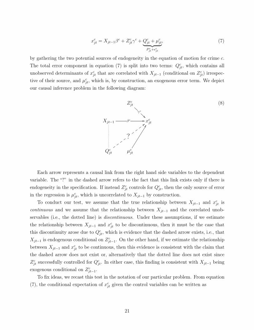
5.3 A Formal Test of Endogeneity

In this section, we present a formal test of exogeneity that we perform on all specifications,which is based on continuity conditions and is inspired by Caetano (2012). We first discussthe intuition behind this test and why it has statistical power to reject the identifyingassumption underlying our analysis. We then describe the test more formally. Equation (2)can be rewritten as

31Note that our findings of higher order within-crime intertemporal effects do not contradict the consistencyof the estimates of �c

1 found in specifications 4-6 in table 2. That is, from an estimation standpoint, aspecification of the system of equations with a single lag is valid. However, when computing dynamicspillovers in the next section, we would like to allow for all intertemporal causal effects, even at higher lags.

20

xc

jt

= Xjt�1�

c + Zc

jt

�c +Qc

jt

+ µc

jt| {z }P

cjt+✏

cjt

, (7)

by gathering the two potential sources of endogeneity in the equation of motion for crime c.The total error component in equation (7) is split into two terms: Qc

jt

, which contains allunobserved determinants of xc

jt

that are correlated with Xjt�1 (conditional on Zc

jt

) irrespec-tive of their source, and µc

jt

, which is, by construction, an exogenous error term. We depictour causal inference problem in the following diagram:

Zc

jt

�

c

X

jt�1 �

c // xc

jt

Qc

jt

?

;;

µc

jt

EE

(8)

Each arrow represents a causal link from the right hand side variables to the dependentvariable. The “?” in the dashed arrow refers to the fact that this link exists only if there isendogeneity in the specification. If instead Zc

jt

controls for Qc

jt

, then the only source of errorin the regression is µc

jt

, which is uncorrelated to Xjt�1 by construction.

To conduct our test, we assume that the true relationship between Xjt�1 and xc

jt

iscontinuous and we assume that the relationship between X

jt�1 and the correlated unob-servables (i.e., the dotted line) is discontinuous. Under these assumptions, if we estimatethe relationship between X

jt�1 and xc

jt

to be discontinuous, then it must be the case thatthis discontinuity arose due to Qc

jt

, which is evidence that the dashed arrow exists, i.e., thatX

jt�1 is endogenous conditional on Zc

jt�1. On the other hand, if we estimate the relationshipbetween X

jt�1 and xc

jt

to be continuous, then this evidence is consistent with the claim thatthe dashed arrow does not exist or, alternatively that the dotted line does not exist sinceZc

jt

successfully controlled for Qc

jt

. In either case, this finding is consistent with Xjt�1 being

exogenous conditional on Zc

jt�1.To fix ideas, we recast this test in the notation of our particular problem. From equation

(7), the conditional expectation of xc

jt

given the control variables can be written as

21

E[xc

jt

|Xjt�1, Z

c

jt

] = Xjt�1�

c + Zc

jt

�c + E[Qc

jt

|Xjt�1, Z

c

jt

] (9)

We decompose the source of endogeneity in equation (7) as32

E⇥Qc

jt

|Xjt�1, Z

c

jt

⇤= �c

Q,X|Z(Djt�1�c +X

jt�1⇡x

+ Zc

jt

⇡z

) (10)

where �c

Q,X|Z ⌘ Cov�Qc

jt

, Xjt�1|Zc

jt

�is a scalar, �c is a C⇥1 vector, and D

jt�1 ⌘�d1jt�1, . . . , d

C

jt�1

�

is a row vector of dummy variables defined as

dcjt�1 = 1 if xc

jt�1 = 0 (11)

= 0 otherwise

Our goal is to design a test of hypothesis:33

H0 : �c

Q,X|Z = 0 for all c

H1 : �c

Q,X|Z 6= 0 for some c

Note that if Zc

jt

contains the fixed effects �c

Jt

and �c

jT

, then H0 implies assumption 1 andH1 implies assumption 1 does not hold.34 Hence this test is a formal, statistical method totest the identifying assumption for specifications 4-6. We can substitute equation (10) intoequation (9), which we rewrite as

E[xc

jt

|Xjt�1, Z

c

jt

] = Xjt�1(�

c + ⇡x

�c

Q,X|Z) + Zc

jt

(�c + ⇡z

�c

Q,X|Z) +Djt�1 �

c�c

Q,X|Z| {z }�

c

(12)

According to equation (12), �c is identified by OLS under H0, but under H1 least squaresestimates of the coefficient on X

jt�1 will be biased. In general, we cannot identify �c

Q,X|Z

in equation (12) in order to test H0. However, we can identify �c ⌘ �c�c

Q,X|Z by simply

32This equation can be written more generally as E⇥Qc

jt|Xjt�1, Zcjt

⇤= �c

Q,X|Z(Djt�1�c + f c(Xjt�1, Z

cjt))

where f c is continuous in Xjt�1, but otherwise unrestricted.33Altonji et al. (2005) describe a different approach to measure the importance of Qc

jt relative to totalexplanatory power of Xjt�1 and Zc

jt. In particular, they offer a method to compute the ratio of the amountof selection on unobservables relative to the amount of selection-on-observables that would be requiredto exist if the entire estimated effect was fully attributed to endogeneity. In addition to different primitiveassumptions, the notable distinction between their approach and ours is that we are able to test the selection-on-observables hypothesis itself. Hence, we can make statements of the form, “we cannot reject exogeneityof Xjt�1 at the ↵̂ level of significance” where ↵̂ is the critical size of the test that we can directly estimate.

34Strictly speaking, the converse (H1 implies assumption 1 does not hold) is true if Zcjt only contains the

fixed effects �cJt and �c

jT as in specification 4.

22

including Djt�1 in a least squares regression of the system of equations. If an estimate of �c

for any c contains at least one non-zero element, then �c

Q,X|Z 6= 0, and we must reject thenull hypothesis of exogeneity. In contrast, if we cannot reject that �c = ~0 for all c, then byextension, we cannot reject the null hypothesis. In order to determine whether �c

Q,X|Z = 0

if we find that �c = ~0, we need to ensure that �c 6= ~0.

Assumption 2. �c 6= ~0 for some c.35

Assumption 2 states that if Qc

jt

exists, it will be discontinuous at xc

0jt�1 for some c0. Note

that if assumption 2 was not satisfied, then this test would not be able to reject the nullhypothesis of exogeneity. Thus, assumption 2 provides power to the test. Intuitively, ifmore elements of �c are different from zero, then this test is more powerful; that is, we canbe more confident that our OLS estimates are unbiased when we do not reject H0. In theonline appendix, we provide theoretical and empirical evidence in favor of assumption 2. Inparticular, we show how this test has power to detect endogeneity due to unobserved policeresponses, (non-classical) measurement error, especially due to misreporting of crime, andother omitted determinants of crime.

To test formally for whether all elements of �1, . . . , �C are equal to zero, we use a jointF-test. For each specification, the F-test provides statistical evidence for the (non)existenceof at least one variable that is wrongly omitted from the specification among all unobservedvariables that vary discontinuously at xc

0jt�1 = 0 for some c0.

In table 2, we present the F-statistic (and p-value) for the test of exogeneity that corre-sponds to each specification. In specifications 1 through 3 we reject the null hypothesis andconclude that the parameter estimates in these specifications are biased. These rejectionsalso show trivially that our test has power to detect endogeneity. On the other hand, inspecifications 4 through 6 we are unable to detect endogeneity with this test, even at highlevels of significance. Finally, in table 5 we perform an even more powerful test of exogeneityby adding D

jt�2, Djt�3 and Djt�4 and by testing whether all (120) of the estimates of the

coefficients of these indicator variables are jointly equal to zero. We are also unable to rejectthe null hypothesis and detect endogeneity in this specification at high levels of significance.In total, this serves as an additional piece of evidence in favor of the claim that the pa-rameter estimates in our preferred specifications correspond to the short run intertemporalbehavioral effects of crime.

35Strictly speaking, we only need this assumption to hold under H1.

23

6 Computing Dynamic Spillovers of Crime

The coefficient estimates in table 5 present the short run effects of light crimes in one weekon all reported crimes in the following 1 to 4 weeks.36 However, prior crimes may indirectlycontinue to affect future crimes of all types over a longer time horizon. Any test of theeffectiveness of the BW policies must consider the long run dynamic effects of crimes, espe-cially light crimes, which include the direct and indirect intertemporal effects both withinand across crimes.

In order to explore these dynamic interactions, we use our coefficient estimates to performan experiment in which we reduce one reported crime of a given type in week 0 and thensimulate the evolution of all reported crimes in weeks 1, 2, . . . holding all else constant. Wethen compute the cumulative change in the levels of all crimes relative to how they wouldhave evolved in the absence of the counterfactual reduction. We interpret the cumulativesimulated changes in future crime levels as the dynamic spillovers that are associated withreductions in current crime levels holding all else constant except the endogenous behavioralresponses to crime.37

We present the cumulative long run spillovers associated with unit reductions of each typeof crime in figure 1 along with 95% confidence intervals.38 The label above each panel refersto the type of crime that we hypothetically reduce by one unit, and the labels for each barrefer to the type of crime that experiences the spillover. Note that the y-axis for rapes is ata different scale from the y-axis for the other crimes, since the estimated spillovers for rapesas an explanatory variable are relatively imprecise. It is immediate that all within-crimedynamic spillovers are statistically significant (except assault) and these spillovers tend tobe large relative to across-crime dynamic spillovers (except rape and assault).

Importantly, we find no statistically significant across-crime dynamic spillovers associatedwith reductions in light crime, which suggests that a BW policy will have little success inreducing the future levels of more severe crimes. For perspective, the dynamic spillover ben-efits associated with a policy that targets either robbery or auto theft strictly dominate thedynamic spillover benefits of a policy that targets light crime, as the across-crime effects of re-ducing robbery and auto theft on future light crimes are of the same order of magnitude as thewithin-crime effect of reducing light crime. A policy that targets assaults generates dynamicspillover reductions in light crime that are smaller than the within-crime spillovers associ-

36The full set of estimates of �ck are presented in the online appendix table 4.

37We report upper bounds on these long run dynamic spillovers as conservative estimates by assumingzero intertemporal discounting.

38Because our system of equations is linear in Xjt�1, . . . , Xjt�⌧ , the cumulative long run spillovers can becomputed analytically. The standard errors for these spillovers are calculated using the delta method, whichaccounts for the correlations among the elements of �c

k for all c and k.

24

ated with light crime reduction, but this policy also generates positive spillover reductionsin future rape and robbery levels. However, this policy generates no within-crime spillover.Even though a policy that targets burglaries does not generate across-crime spillovers, itgenerates the largest within-crime positive spillovers of all of the crimes.39

Although figure 1 offers insight into the statistical significance of our results and thetrade-offs involved in targeting each crime, it is difficult to glean the economic significance ofthese dynamic spillovers. To provide this context, we conduct a simple thought experiment.First, we consider an average neighborhood in an average week of our sample. In thisneighborhood, we perform a hypothetical intervention in which we fully eliminate all crimesof type c for a week and compute the total cumulative long run spillovers within and acrossall crimes as t ! 1. We then express this long run dynamic spillover effect on crimes as afraction of the average weekly crime level in the neighborhood. The results of this exerciseallow us to construct an upper bound on the efficacy of a targeted city-wide intervention. Wepresent the cumulative reductions in crimes from these interventions in table 6. For example,a complete elimination of light crime in the average neighborhood for one week (a reductionof 23.15 light crimes) generates a total future spillover reduction in rapes equal to only 9.5%of the average number of weekly rapes in the neighborhood (a cumulative reduction of 0.03future rapes).

Three results are immediate from table 6. First, within-crime dynamic spillovers tendto be relatively large (except assault) and are precisely estimated. Second, across-crimedynamic spillovers from light crime reduction are both small and statistically insignificant,as even a full elimination of light crimes generates at most modest future reductions in moresevere crimes (less than 10%). Third, across crime spillovers from policies that reduce othercrimes are small and largely statistically insignificant.

In sum, these findings suggests that a BW law enforcement policy based on aggressivelytargeting light crimes will fail to reduce the future rates of more severe crimes in an econom-ically significant way.

6.1 Cost-Benefit Analysis

Even if a BW law enforcement policy that targets light crimes is not effective in reducingfuture severe crime rates, it may still be an optimal policy from a cost-benefit perspective. Weexpand on this point by performing a back of the envelope evaluation of the monetary benefits

39We are hesitant to assess the benefits of a hypothetical policy that targets rape due to imprecision inour estimates of the dynamic spillovers associated with such a policy. The inclusion of rape in our analysisis important because we are able to precisely estimate the intertemporal effects of other crimes on rape. Theresults do not change when we drop rape from the analysis.

25

of various crime reduction policies. In table 7, we present estimates of the monetary benefitsof a unit crime reduction.40 In the first column, we list the social benefits of reducing one unitof each type of crime that we adapt from Heaton (2010) and supplement with Miller et al.(1993).41 These estimates of the social costs of each type of crime are designed to accountfor both tangible and intangible costs of crime. Tangible costs include direct financial coststo individuals, businesses and governments including productivity losses. Intangible costsinclude losses in quality of life due to fear of crime and the psychological costs of victimization.

In the second column of table 7, we compute the total monetary benefits that are associ-ated with a law enforcement policy that reduces one unit of a particular type of crime. Wecalculate these by simulating the dynamic spillover changes in all crimes associated with aunit reduction of a particular type of crime, valuing them according to the figures in column1, and adding them to the direct benefit of the unit reduction. For example, a policy thatreduces one robbery generates roughly $86,000 in total social benefits in present value. Onthe other hand, a BW law enforcement policy that reduces one unit of light crime generatesonly $3,341 in total social benefits in present value.42

A simple comparison of the benefits of crime reduction policies is incomplete without aconcomitant consideration of the costs of implementing these policies. Unfortunately, we areunable to find external estimates of the marginal costs of abating specific crimes.43 Nev-ertheless, we can still offer a rough policy prescription. In the third column of table 7, wepresent the total current and future benefits of unit crime reduction policies in terms of thesame benefits associated with a unit light crime reduction policy. Unless the marginal costof reducing robbery is more than 25.88 times the marginal cost of reducing light crime, apolicy targeting robberies is preferable from a cost-benefit perspective to a BW law enforce-ment policy, and unless the marginal cost of reducing burglary is more than 7.06 times themarginal cost of reducing light crime, a policy targeting burglaries is preferable to a BW lawenforcement policy. Similar results for the remaining crimes are presented in the table.

40All monetary values are presented in 2012 dollars.41Details of the construction of these cost estimates can be found in the footnote to table 7.42These estimated benefits are based on an analysis of only six types of crime; to the extent that reductions

in these six crimes generate dynamic spillovers across other types of crimes (e.g., murder) in the future, wewill underestimate the social benefits of any crime reduction. However, we believe these results are (ifanything) biased in favor of finding support for BW policies because we expressly selected those crimes forwhich social learning is likely to matter.

43We believe this inability highlights the lack of attention to the net benefits of law enforcement policiesin the literature so far.

26

7 Conclusion

The “Broken Windows” theory of crime has influenced urban law enforcement policy overthe past twenty years in many cities. Although there has been a vibrant debate in the policyarena over its desirability and efficacy, surprisingly little work has been done to empiricallyvalidate such theory. In this paper, we offer robust empirical evidence against this theory.

The primary policy content of BW follows from the notion that less severe crimes willendogenously lead to more severe crimes being committed in the future. Under this assump-tion, a law enforcement agency utilizing BW policing techniques ought to divert policingattention and resources preferentially from more severe crimes to less severe crimes in orderto take advantage of this dynamic spillover. Our analysis casts substantial doubt on the ef-fectiveness of such a policy in abating more severe crimes, as we consistently find no evidencethat a reduction of light crime leads to future reductions in the levels of more severe crimes.Instead, if an agency aims to reduce the levels of severe crimes, our analysis supports lawenforcement policies that aggressively target severe crimes. Indeed, the evidence of dynamicspillovers from higher intensity crimes to light crime that we find suggests that the spilloverbenefits of such policies will strictly dominate the spillover benefits of a BW policy. Wealso find in a cost-benefit analysis that unless the marginal costs of combating severe crimesexceed the marginal costs of combating light crimes by a factor of at least 25 for robberyand 7 for burglary, BW policing is likely inefficient in addition to being ineffective.

We conclude by noting that further inquiry into the costs and benefits of targeted lawenforcement policies is well warranted. Such information would allow for a fuller welfareanalysis of law enforcement policy and could provide more precise and comprehensive pre-scriptions to policymakers.

References

Akerlof, G., 1997. Social distance and social decisions. Econometrica: Journal of the Econo-metric Society, 1005–1027.

Altonji, J., Elder, T., Taber, C., 2005. Selection on observed and unobserved variables:Assessing the effectiveness of catholic schools. Journal of Political Economy 113 (1), 151–184.

Angrist, J., Pischke, J., 2009. Mostly harmless econometrics: An empiricist’s companion.Princeton Univ Pr.

Arrow, K., 1962. The economic implications of learning by doing. The review of economicstudies, 155–173.

27

Banerjee, A., 1992. A simple model of herd behavior. The Quarterly Journal of Economics107 (3), 797–817.

Becker, G., 1968. Crime and punishment: An economic approach. The Journal of PoliticalEconomy 76 (2), 169–217.

Becker, G., 1974. A theory of social interactions. The Journal of Political Economy 82 (6),1063–1093.

Bikhchandani, S., Hirshleifer, D., Welch, I., 1992. A theory of fads, fashion, custom, andcultural change as informational cascades. Journal of political Economy, 992–1026.

Bikhchandani, S., Hirshleifer, D., Welch, I., 1998. Learning from the behavior of others: Con-formity, fads, and informational cascades. The Journal of Economic Perspectives 12 (3),151–170.

Block, R., 1993. A cross-national comparison of victims of crime: victim surveys of twelvecountries. International Review of Victimology 2 (3), 183–207.

Braga, A., Bond, B., 2008. Policing crime and disorder hot spots: A randomized controlledtrial*. Criminology 46 (3), 577–607.

Bronars, S., Lott Jr, J., 1998. Criminal deterrence, geographic spillovers, and the right tocarry concealed handguns. American Economic Review, 475–479.

Caetano, C., 2012. A test of exogeneity without instrumental variables. mimeo.

Caetano, G., Maheshri, V., 2012. School segregation and the identification of tipping points.Working Paper.

Calvo-Armengol, A., Zenou, Y., 2004. Social networks and crime decisions: The role ofsocial structure in facilitating delinquent behavior. International Economic Review 45 (3),939–958.

Card, D., Dobkin, C., Maestas, N., 2008. The impact of nearly universal insurance coverageon health care utilization: Evidence from medicare. American Economic Review 98, 2242–2258.

Corman, H., Mocan, N., 2005. Carrots, sticks, and broken windows. Journal of Law andEconomics, 48.

Cornish, D., Clarke, R., 1987. Understanding crime displacement: An application of rationalchoice theory. Criminology 25 (4), 933–948.

28

Davis, M., 1988. Time and punishment: an intertemporal model of crime. The Journal ofPolitical Economy, 383–390.

Dube, A., Lester, T., Reich, M., 2010. Minimum wage effects across state borders: Estimatesusing contiguous counties. The review of economics and statistics 92 (4), 945–964.

Ellison, G., Fudenberg, D., 1995. Word-of-mouth communication and social learning. TheQuarterly Journal of Economics 110 (1), 93–125.

Fajnzlber, P., Lederman, D., Loayza, N., 2002. Inequality and violent crime. JL & Econ. 45,1.

Fajnzylber, P., Lederman, D., Loayza, N., 2002. What causes violent crime? EuropeanEconomic Review 46 (7), 1323–1357.

Fender, J., 1999. A general equilibrium model of crime and punishment. Journal of EconomicBehavior & Organization 39 (4), 437–453.

Flango, V. E., Sherbenou, E. L., 1976. Poverty, urbanization, and crime. Criminology 14 (3),331–346.

Funk, P., Kugler, P., 2003. Dynamic interactions between crimes. Economics Letters 79 (3),291–298.

Gale, D., 1996. What have we learned from social learning? European Economic Review40 (3), 617–628.

Gladwell, M., 2000. The tipping point: How little things can make a big difference. Little,Brown and Company.

Glaeser, E., Sacerdote, B., Scheinkman, J., 1996. Crime and social interactions. The Quar-terly Journal of Economics, 507–548.

Gul, F., Lundholm, R., 1995. Endogenous timing and the clustering of agents’ decisions.Journal of Political Economy, 1039–1066.

Harcourt, B., 1998. Reflecting on the subject: A critique of the social influence conceptionof deterrence, the broken windows theory, and order-maintenance policing new york style.Michigan Law Review 97 (2), 291–389.

Harcourt, B., Ludwig, J., 2006. Broken windows: New evidence from new york city and afive-city social experiment. The University of Chicago Law Review, 271–320.

29

Heaton, P., 2010. Hidden in Plain Sight. RAND Corporation.

Imai, S., Krishna, K., 2004. Employment, deterrence, and crime in a dynamic model*.International Economic Review 45 (3), 845–872.

Jackson, M., Watts, A., 2002. The evolution of social and economic networks. Journal ofEconomic Theory 106 (2), 265–295.

Jacob, B., Lefgren, L., Moretti, E., 2007. The dynamics of criminal behavior: Evidence fromweather shocks. Journal of Human Resources 42 (3), 489–527.

Keizer, K., Lindenberg, S., Steg, L., 2008. The spreading of disorder. Science 322 (5908),1681–1685.

Kelling, G., Coles, C., 1998. Fixing broken windows: Restoring order and reducing crime inour communities. Free Press.

Kelling, G., Sousa, W., 2001. Do Police Matter?: An Analysis of the Impact of New YorkCity’s Police Reforms. CCI Center for Civic Innovation at the Manhattan Institute.

Kempf, K., 1987. Specialization and the criminal career. Criminology 25 (2), 399–420.

Lade, S. J., Gross, T., 2012. Early warning signals for critical transitions: A generalizedmodeling approach. PLoS computational biology 8 (2), e1002360.

Lee, D., McCrary, J., 2005. Crime, punishment, and myopia. Tech. rep., National Bureau ofEconomic Research.

Levitt, S., 1998. Why do increased arrest rates appear to reduce crime: deterrence, incapac-itation, or measurement error? Economic Inquiry 36 (3), 353–372.

Levitt, S., 2004. Understanding why crime fell in the 1990s: Four factors that explain thedecline and six that do not. The Journal of Economic Perspectives 18 (1), 163–190.

Manski, C., 2000. Economic analysis of social interactions. Journal of Economic Perspectives14 (3), 115–136.

Miller, T., Cohen, M., Rossman, S., 1993. Victim costs of violent crime and resulting injuries.Health Affairs 12 (4), 186–197.

Morenoff, J., Sampson, R., 1997. Violent crime and the spatial dynamics of neighborhoodtransition: Chicago, 1970–1990. Social forces 76 (1), 31–64.

30

Mosher, C., Hart, T., Miethe, T., 2010. The mismeasure of crime. Sage Publications, Inc.

Sampson, R. J., 1985. Neighborhood and crime: The structural determinants of personalvictimization. Journal of Research in Crime and Delinquency 22 (1), 7–40.

Sherman, L., Weisburd, D., 1995. General deterrent effects of police patrol in crime ’hotspots’: A randomized, controlled trial. Justice Quarterly 12 (4), 625–648.

Skogan, W., 1974. The validity of official crime statistics: An empirical investigation. SocialScience Quarterly 55 (1), 25–38.

Skogan, W., 1975. Measurement problems in official and survey crime rates. Journal ofCriminal Justice 3 (1), 17–31.

Skogan, W., 1977. Dimensions of the dark figure of unreported crime. Crime & Delinquency23 (1), 41–50.

Taylor, R., 1996. Neighborhood responses to disorder and local attachments: The systemicmodel of attachment, social disorganization, and neighborhood use value. In: SociologicalForum. Vol. 11. Springer, pp. 41–74.

Thibaut, J., Kelley, H., 1959. The social psychology of groups.

Weisburd, D., Eck, J., 2004. What can police do to reduce crime, disorder, and fear? TheAnnals of the American Academy of Political and Social Science 593 (1), 42–65.

Zellner, A., 1962. An efficient method of estimating seemingly unrelated regressions and testsfor aggregation bias. Journal of the American statistical Association, 348–368.

Zimring, F., 1998. Youth violence epidemic: Myth or reality, the. Wake Forest L. Rev. 33,727.

31

Table 1: Summary Statistics: 2000-2007

Variable Rape Robbery Burglary Auto

Theft

Assault Light

Crime

Average reported crimes in a

sector per week

0.42

(0.69)

4.58

(3.18)

13.30

(7.56)

10.71

(6.01)

21.29

(12.07)

23.15

(10.15)

Average police response time

(hours)

2.37

(1.45)

1.29

(1.00)

1.39

(0.73)

0.88

(0.66)

1.38

(0.74)

1.41

(0.72)

Average police duration (hours) 1.08

(1.61)

0.97

(1.73)

0.59

(0.81)

0.41

(0.68)

0.67

(0.71)

0.62

(0.61)

Share of crimes committed at

night

0.62 0.55 0.36 0.50 0.45 0.43

Share of crimes committed

outdoors

0.26 0.59 0.02 0.79 0.33 0.58

Share of crimes committed on the

weekend

0.35 0.33 0.24 0.30 0.35 0.29

Share of crimes reported by

private businesses

0.00 0.20 0.34 0.06 0.00 0.10

Total reported crimes 5,439 59,015 171,506 138,086 274,586 298,520

Notes: Standard deviations are presented in parentheses where relevant. Average police response time is measured in hours

from dispatch time to officer’s arrival. Average police duration is measured in hours from officer’s arrival to the scene of the

crime to their departure. Night crimes occur between 8:00PM and 8:00AM of the following day.

32

Table 2: Intertemporal Behavioral Effects of Light Crime

Dep. Var. (t) (1) (2) (3) (4) (5) (6)

Rape -0.006

(0.001)

0.002**

(0.001)

0.002

(0.001)

0.002

(0.001)

0.002

(0.001)

0.002

(0.001)

Robbery 0.013

(0.014)

0.017**

(0.005)

0.018**

(0.004)

0.003

(0.004)

0.003

(0.004)

0.003

(0.004)

Burglary 0.088**

(0.010)

0.085**

(0.010)

0.045**

(0.008)

0.006

(0.009)

0.007

(0.009)

0.007

(0.009)

Auto Theft 0.088**

(0.009)

0.095**

(0.010)

0.040**

(0.008)

0.009

(0.008)

0.008

(0.009)

0.008

(0.008)

Assault 0.148**

(0.012)

0.159**

(0.013)

0.101**

(0.012)

0.016

(0.010)

0.016

(0.010)

0.015

(0.010)

Light Crime 0.436**

(0.017)

0.412**

(0.017)

0.182**

(0.014)

0.066**

(0.014)

0.065**

(0.014)

0.065**

(0.014)

All other crimes in t� 1 included? Yes Yes Yes Yes Yes Yes

Year-Crime type FE included? No Yes No No No No

Sector-Crime type FE included? No No Yes No No No

Week-Crime type FE included? No No Yes No No No

Sector-Year-Crime type FE included? No No No Yes Yes Yes

Division-Week-Crime type FE included? No No No Yes Yes Yes

Controlled for frac. of each crime type

at t� 1 at daytime?

No No No No Yes Yes

Controlled for frac. of each crime type

at t� 1 on the weekend?

No No No No Yes Yes

Controlled for frac. of each crime type

at t� 1 outdoors?

No No No No Yes Yes

Average police response time at t for

each crime type included?

No No No No No Yes

Average police duration at t for each

crime type included?

No No No No No Yes

R

2 0.810 0.812 0.851 0.867 0.867 0.867

Discontinuity test F-statistic (P value) 11.14**

(0.00)

1.85**

(0.00)

1.46*

(0.05)

0.90

(0.62)

0.85

(0.70)

0.87

(0.67)

Number of observations 12,864 12,864 12,864 12,864 12,864 12,864

Notes: This table shows the coefficient estimates of light crime in period t � 1 for each dependent variable in period t, as in

equation (5). Heteroskedasticity robust standard errors clustered by sector-year-crime type are presented in parentheses. *:

significant at 5% level. **: significant at 1% level. The other coefficient estimates of the regression are presented in table 1 in

the online appendix.

33

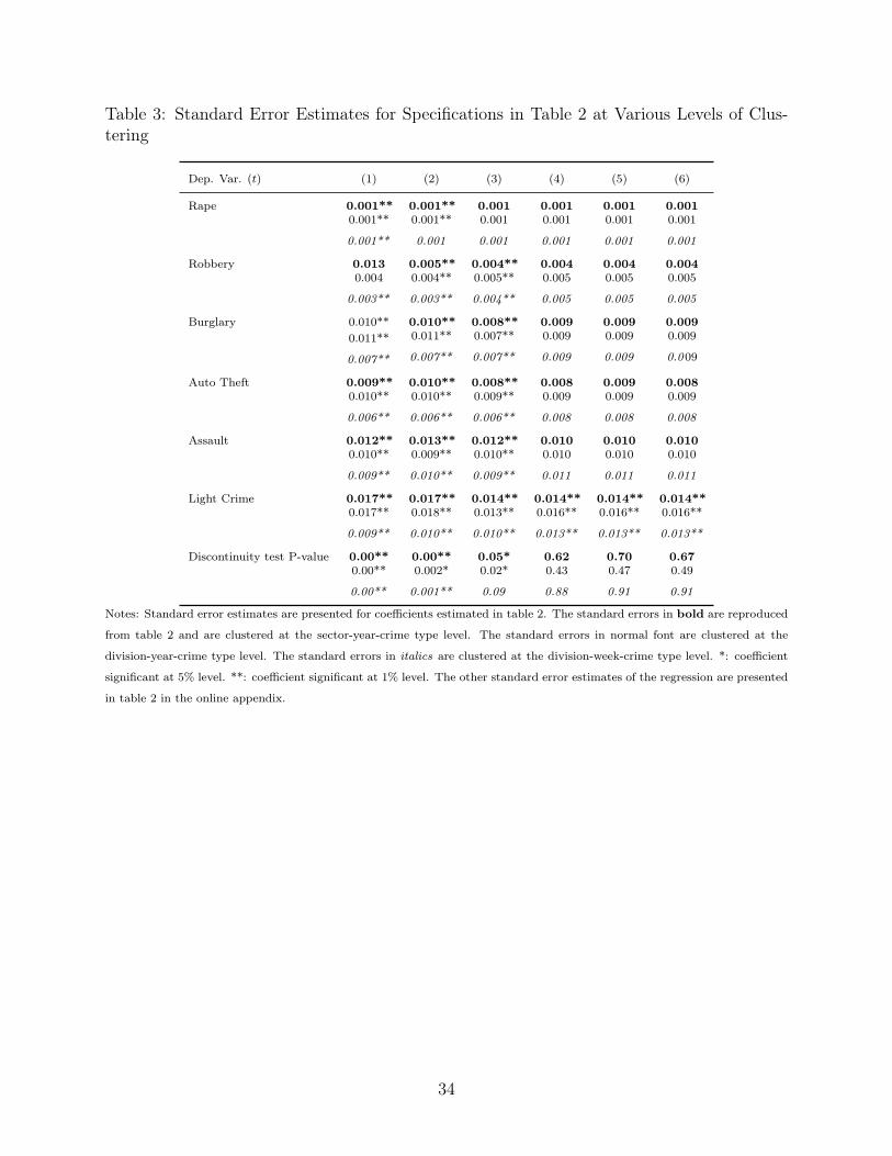
Table 3: Standard Error Estimates for Specifications in Table 2 at Various Levels of Clus-tering

Dep. Var. (t) (1) (2) (3) (4) (5) (6)

Rape 0.001**

0.001**

0.001**

0.001**

0.001**

0.001

0.001

0.001

0.001

0.001

0.001

0.001

0.001

0.001

0.001

0.001

0.001

0.001

Robbery 0.013

0.004

0.003**

0.005**

0.004**

0.003**

0.004**

0.005**

0.004**

0.004

0.005

0.005

0.004

0.005

0.005

0.004

0.005

0.005

Burglary 0.010**0.011**

0.007**

0.010**

0.011**

0.007**

0.008**

0.007**

0.007**

0.009

0.009

0.009

0.009

0.009

0.009

0.009

0.009

0.009

Auto Theft 0.009**

0.010**

0.006**

0.010**

0.010**

0.006**

0.008**

0.009**

0.006**

0.008

0.009

0.008

0.009

0.009

0.008

0.008

0.009

0.008

Assault 0.012**

0.010**

0.009**

0.013**

0.009**

0.010**

0.012**

0.010**

0.009**

0.010

0.010

0.011

0.010

0.010

0.011

0.010

0.010

0.011

Light Crime 0.017**

0.017**

0.009**

0.017**

0.018**

0.010**

0.014**

0.013**

0.010**

0.014**

0.016**

0.013**

0.014**

0.016**

0.013**

0.014**

0.016**

0.013**

Discontinuity test P-value 0.00**

0.00**

0.00**

0.00**

0.002*

0.001**

0.05*

0.02*

0.09

0.62

0.43

0.88

0.70

0.47

0.91

0.67

0.49

0.91

Notes: Standard error estimates are presented for coefficients estimated in table 2. The standard errors in bold are reproduced

from table 2 and are clustered at the sector-year-crime type level. The standard errors in normal font are clustered at the

division-year-crime type level. The standard errors in italics are clustered at the division-week-crime type level. *: coefficient

significant at 5% level. **: coefficient significant at 1% level. The other standard error estimates of the regression are presented

in table 2 in the online appendix.

34

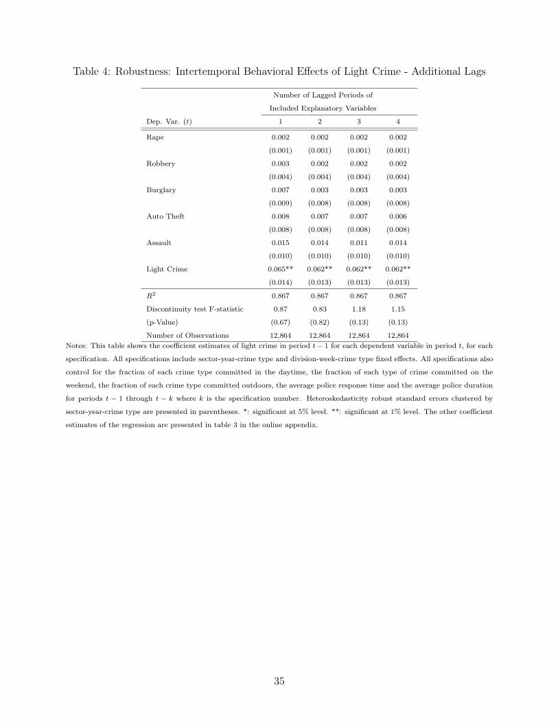
Table 4: Robustness: Intertemporal Behavioral Effects of Light Crime - Additional Lags

Number of Lagged Periods of

Included Explanatory Variables

Dep. Var. (t) 1 2 3 4

Rape 0.002

(0.001)

0.002

(0.001)

0.002

(0.001)

0.002

(0.001)

Robbery 0.003

(0.004)

0.002

(0.004)

0.002

(0.004)

0.002

(0.004)

Burglary 0.007

(0.009)

0.003

(0.008)

0.003

(0.008)

0.003

(0.008)

Auto Theft 0.008

(0.008)

0.007

(0.008)

0.007

(0.008)

0.006

(0.008)

Assault 0.015

(0.010)

0.014

(0.010)

0.011

(0.010)

0.014

(0.010)

Light Crime 0.065**

(0.014)

0.062**

(0.013)

0.062**

(0.013)

0.062**

(0.013)

R

2 0.867 0.867 0.867 0.867

Discontinuity test F-statistic

(p-Value)

0.87

(0.67)

0.83

(0.82)

1.18

(0.13)

1.15

(0.13)

Number of Observations 12,864 12,864 12,864 12,864Notes: This table shows the coefficient estimates of light crime in period t� 1 for each dependent variable in period t, for each

specification. All specifications include sector-year-crime type and division-week-crime type fixed effects. All specifications also

control for the fraction of each crime type committed in the daytime, the fraction of each type of crime committed on the

weekend, the fraction of each crime type committed outdoors, the average police response time and the average police duration

for periods t � 1 through t � k where k is the specification number. Heteroskedasticity robust standard errors clustered by

sector-year-crime type are presented in parentheses. *: significant at 5% level. **: significant at 1% level. The other coefficient

estimates of the regression are presented in table 3 in the online appendix.

35

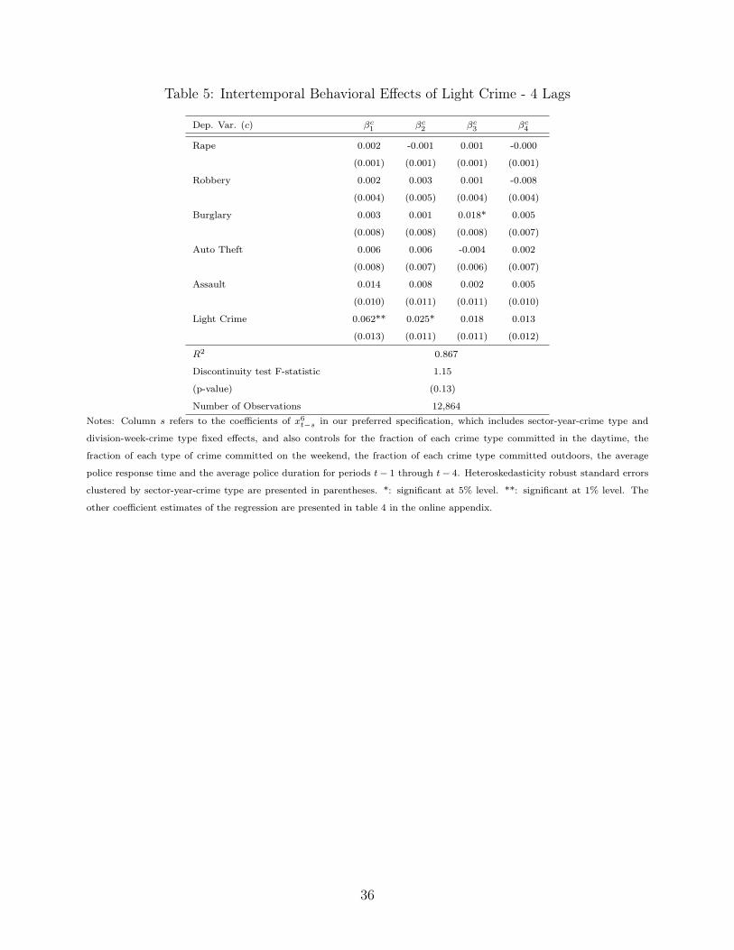
Table 5: Intertemporal Behavioral Effects of Light Crime - 4 Lags

Dep. Var. (c) �

c1 �

c2 �

c3 �

c4

Rape 0.002

(0.001)

-0.001

(0.001)

0.001

(0.001)

-0.000

(0.001)

Robbery 0.002

(0.004)

0.003

(0.005)

0.001

(0.004)

-0.008

(0.004)

Burglary 0.003

(0.008)

0.001

(0.008)

0.018*

(0.008)

0.005

(0.007)

Auto Theft 0.006

(0.008)

0.006

(0.007)

-0.004

(0.006)

0.002

(0.007)

Assault 0.014

(0.010)

0.008

(0.011)

0.002

(0.011)

0.005

(0.010)

Light Crime 0.062**

(0.013)

0.025*

(0.011)

0.018

(0.011)

0.013

(0.012)

R

2 0.867

Discontinuity test F-statistic

(p-value)

1.15

(0.13)

Number of Observations 12,864Notes: Column s refers to the coefficients of x

6t�s in our preferred specification, which includes sector-year-crime type and

division-week-crime type fixed effects, and also controls for the fraction of each crime type committed in the daytime, the

fraction of each type of crime committed on the weekend, the fraction of each crime type committed outdoors, the average

police response time and the average police duration for periods t� 1 through t� 4. Heteroskedasticity robust standard errors

clustered by sector-year-crime type are presented in parentheses. *: significant at 5% level. **: significant at 1% level. The

other coefficient estimates of the regression are presented in table 4 in the online appendix.

36

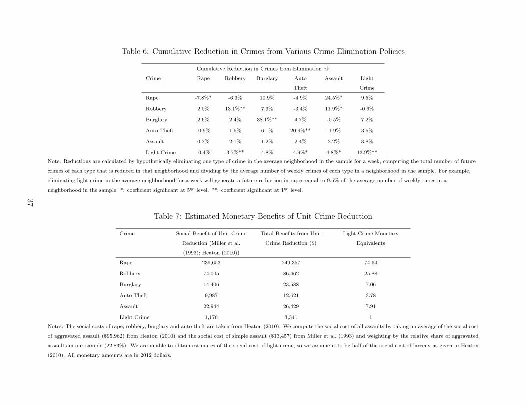
Table 6: Cumulative Reduction in Crimes from Various Crime Elimination Policies

Cumulative Reduction in Crimes from Elimination of:

Crime Rape Robbery Burglary Auto

Theft

Assault Light

Crime

Rape -7.8%* -6.3% 10.9% -4.9% 24.5%* 9.5%

Robbery 2.0% 13.1%** 7.3% -3.4% 11.9%* -0.6%

Burglary 2.6% 2.4% 38.1%** 4.7% -0.5% 7.2%

Auto Theft -0.9% 1.5% 6.1% 20.9%** -1.9% 3.5%

Assault 0.2% 2.1% 1.2% 2.4% 2.2% 3.8%

Light Crime -0.4% 3.7%** 4.8% 4.9%* 4.8%* 13.9%**

Note: Reductions are calculated by hypothetically eliminating one type of crime in the average neighborhood in the sample for a week, computing the total number of future

crimes of each type that is reduced in that neighborhood and dividing by the average number of weekly crimes of each type in a neighborhood in the sample. For example,

eliminating light crime in the average neighborhood for a week will generate a future reduction in rapes equal to 9.5% of the average number of weekly rapes in a

neighborhood in the sample. *: coefficient significant at 5% level. **: coefficient significant at 1% level.

Table 7: Estimated Monetary Benefits of Unit Crime Reduction

Crime Social Benefit of Unit Crime

Reduction (Miller et al.

(1993); Heaton (2010))

Total Benefits from Unit

Crime Reduction ($)

Light Crime Monetary

Equivalents

Rape 239,653 249,357 74.64

Robbery 74,005 86,462 25.88

Burglary 14,406 23,588 7.06

Auto Theft 9,987 12,621 3.78

Assault 22,944 26,429 7.91

Light Crime 1,176 3,341 1

Notes: The social costs of rape, robbery, burglary and auto theft are taken from Heaton (2010). We compute the social cost of all assaults by taking an average of the social cost

of aggravated assault ($95,962) from Heaton (2010) and the social cost of simple assault ($13,457) from Miller et al. (1993) and weighting by the relative share of aggravated

assaults in our sample (22.83%). We are unable to obtain estimates of the social cost of light crime, so we assume it to be half of the social cost of larceny as given in Heaton

(2010). All monetary amounts are in 2012 dollars.

37

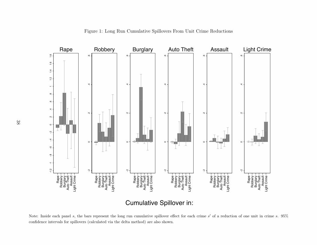
Figure 1: Long Run Cumulative Spillovers From Unit Crime Reductions

-1.2

-1-.8

-.6-.4

-.20

.2.4

.6.8

11.

21.

41.

61.

8

Rap

eR

obbe

ryBu

rgla

ryAu

to T

heft

Assa

ult

Ligh

t Crim

e

Rape

-.20

.2.4

.6

Rap

eR

obbe

ryBu

rgla

ryAu

to T

heft

Assa

ult

Ligh

t Crim

e

Robbery

-.20

.2.4

.6

Rap

eR

obbe

ryBu

rgla

ryAu

to T

heft

Assa

ult

Ligh

t Crim

e

Burglary

-.20

.2.4

.6

Rap

eR

obbe

ryBu

rgla

ryAu

to T

heft

Assa

ult

Ligh

t Crim

e

Auto Theft

-.20

.2.4

.6

Rap

eR

obbe

ryBu

rgla

ryAu

to T

heft

Assa

ult

Ligh

t Crim

e

Assault

-.20

.2.4

.6

Rap

eR

obbe

ryBu

rgla

ryAu

to T

heft

Assa

ult

Ligh

t Crim

e

Light Crime

Cumulative Spillover in:

Note: Inside each panel s, the bars represent the long run cumulative spillover effect for each crime s0 of a reduction of one unit in crime s. 95%confidence intervals for spillovers (calculated via the delta method) are also shown.

38

A APPENDIX

A.1 Detecting Endogeneity

In this appendix we provide theoretical and empirical support for assumption 2 by arguingthat unobservable determinants of crime, measurement error and unobserved police responsesto prior crimes (as well as other potential confounders) all vary discontinuously with xc

0jt�1

at xc

0jt�1 = 0. In section A.1.1, we provide theoretical reasons for this discontinuity to occur,

based on a mechanical bunching of observations at xc

0jt�1 = 0. In section A.1.2, we supplement

this argument with indirect empirical evidence in favor of assumption 2. Taken together,this ensures that our test has power to detect endogeneity from several different sources.

A.1.1 Theoretical Support for Assumption 2

Our general theoretical argument for how discontinuities in Qc

jt

arise is based on the simplefact that that reported crimes are truncated at zero.44 That is, there cannot be a negativenumber of reported crimes in any neighborhood. In general, this truncation will generatebunching of latent variables at the threshold of xc

0jt�1 = 0. To develop this argument and

connect it to our application, we separately consider why omitted endogenous variables ofthree specific types will vary discontinuously at xc

0jt�1 = 0 for some c0. However, we should

note that this is not an exhaustive list of sources of endogeneity that our test can detect, asan analogous argument may also work for other sources of endogeneity.

Figure 1 illustrates a hypothetical relationship between a generic explanatory variable,xc

0jt�1, and a particular unobservable determinant of past crime, e.g., the average neighbor-

hood wealth in period t � 1, which is included in ✏cjt�1. From the first panel of the figure,

poorer neighborhoods are expected to have higher levels of reported crime, but in wealthierneighborhoods reported crime is expected to be lower. When the level of wealth is ✏?, nocrimes are reported in expectation. For any neighborhood with an average wealth larger than✏?, the expected level of reported crime will still be 0, as it cannot be negative. Conversely,we can plot the expected value of neighborhood wealth for each level of reported crime,as in the second panel of the figure. Here, we find a mechanically generated discontinuityin expected wealth when no crimes are reported: neighborhoods with no reported crimesinclude not only those with ✏c

jt�1 = ✏? but also those with ✏cjt�1 > ✏?. Intuitively, there are

44Note that this is distinct from the statement that reported crimes are censored at zero. Indeed, noobserved variables in our analysis are censored at any value. Caetano (2012) discusses this distinction indetail.

39

neighborhoods that are so wealthy that even if they were slightly poorer, no crimes wouldbe reported in expectation.

As another example, we illustrate a hypothetical relationship between xc

0jt�1 and the

propensity of neighborhood residents to misreport crime in period t� 1 in figure 2. When acrime occurs, residents decide whether or not to report it to the police, hence this variable isan important determinant of measurement error. If poorer neighborhoods are more distrust-ful of law enforcement, or if property crimes committed in poorer neighborhoods are of lowervalue, then there would be greater misreporting in poor neighborhoods than in richer neigh-borhoods (Skogan (1977)). In conjunction with the previous example, this suggests that thepropensity to misreport crime may be positively correlated with the level of reported crime.In the first panel of figure 2, neighborhoods that are more likely to misreport crime are shownto suffer from higher expected levels of reported crime. When the propensity to misreport islow enough (i.e., ✏c

jt�1 = ✏?), no crimes are reported in expectation. For any neighborhoodwith a lower propensity to misreport than ✏?, the expected reported level of crime will stillbe zero. This implies a discontinuity in the conditional expectation of the unobservable atthe level of reported crime equals to 0, as shown in the second panel. Intuitively, in someneighborhoods nearly every crime that is committed is reported, and even if a few peoplebegan to harbor distrust of the police, the lack of actual crime in the neighborhood wouldstill lead to no crimes being reported.

We add three remarks about the generality of the argument illustrated by these twoexamples. First, because our system of equations are specified on a panel with geographicand temporal dimensions, any bunching of observations (as opposed to bunching of neigh-borhoods) at xc

0jt�1 = 0 for some c0 will generate a discontinuity similar to the one described

in assumption 2. For instance, if a particular neighborhood has a higher level of some unob-served amenity in the first week of every month (say, because of a monthly farmer’s market),then this unobservable amenity will vary discontinuously at xc

0jt�1 = 0 for some c0. Second,

the relationship between the unobservable and xc

0jt�1 need not be monotonic as illustrated in

these figures, nor does the discontinuity need to lie in the direction of the slope of xc

0jt�1 near

xc

0jt�1 = 0. Finally, a sufficient (but not necessary) condition for assumption 2 to hold is that

Qc

jt

is caused by some unobservable that causes xc

0jt�1.45 This guarantees that the bunching

of observations with no reported crime (xc

0jt�1 = 0) will generate a discontinuity in Qc

jt

inexpectation.46

45In figure 1, ✏cjt�1 is not included in Qcjt. However, Qc

jt contains ✏cjt, so any serial correlation in neighbors’wealth will generate a discontinuity in Qc

jt.46The only instance in which assumption 2 does not hold is if Qc

jt is a discontinuous function of theunobservable at precisely the point at which that unobservable causes xc0

jt�1 = 0 (denoted as ✏? in figures 1and 2) and that the size of this discontinuity exactly offsets the original discontinuity of the unobservable.

40

Following the logic of the examples above, the police response to past crimes, P c

jt

, maybe discontinuous at xc

0jt�1 = 0 if it is caused by P c

jt�1. Indeed, the presence of police mayaffect the reporting of crime directly by deterrence or indirectly by mitigating measurementerror, so any inertia in the allocation of police resources would imply a discontinuity in P c

jt

at xc

0jt�1 = 0. The police response may be discontinuous for a second reason: P c

jt

itselfmay be caused by X

jt�1 discontinuously at xc

0jt�1 = 0. Consider for instance the level of

attention that the police give to a neighborhood. Prior reported crimes may cause a changein this unobservable (e.g., due to a police crackdown). Hence, we would expect a positiverelationship between xc

0jt�1 for some c0 and the unobservable police response P c

jt

, as illustratedin figure 3. When fewer crimes are reported, the police tend to reduce their attention in thefollowing period.47 Because the police observe only reported crimes as opposed to actualcrimes, the response of the police to prior reported crimes could be discontinuously differentwhen there is no crime reported versus when there is one crime reported simply because thelack of reported crime in a neighborhood may leave it “under the radar” for that week.

A.1.2 Empirical Support for Assumption 2

In addition to the theoretical arguments laid out in support of assumption 2, we provideindirect empirical evidence in the form of discontinuity plots (figure 4).48 Each point in theseplots represents the mean of the variable on the y-axis (some other potential determinantof current crime levels, such as another element of X

jt�1 or an element of Zc

jt�1 for some c)conditional on a given level of xc

0jt�1 for some c0. The dashed curve represents a third order

local polynomial regression of all of these points for which xc

0jt�1 > 0, and the shaded region

represents the 95% confidence region for this regression, with an out of sample predictionat xc

0jt�1 = 0.49 Finally, the hollow point represents the observed mean value of the variable

on the y-axis conditional on xc

0jt�1 = 0. If the hollow point lies outside of the shaded region,

then this implies that the observed variable on the y-axis is discontinuous at xc

0jt�1 = 0 with

47There may also be a substitution effect as resources are re-allocated to prevent other types of crime.In this case, we may observe a negative relationship between prior reported crime and policing for c 6= c0.Regardless, our test is motivated only by the existence of this relationship, not by its sign.

48This empirical evidence in support of assumption 2 is analogous to the evidence supplied in a standardregression discontinuity (RD) framework in support of the identifying assumption that unobservables varycontinuously at the threshold. Although researchers operating in an RD framework are unable to show thatall unobservable determinants of the outcome vary continuously at the threshold, in practice they showthat many observable determinants of the outcome vary continuously at the threshold. This constitutesindirect evidence that unobservables also vary continuously at the threshold. Similarly, in order to supportassumption 2, we show that a variety of observables vary discontinuously at the threshold.

49For each regression, we use the Epanechnikov kernel with bandwidths of five for the kernel and thestandard error calculation.

41

at least 95% confidence, which is evidence in support of the validity of assumption 2. Indeed,we show that there is ample evidence of discontinuities for various potential determinants ofxc

jt

.50 Although we cannot formally assess why the discontinuities arise in each figure, ourtest only requires that they exist, irrespective of the reason. Nevertheless, we offer suggestiveexplanations for these discontinuities with the intention of providing intuition for our test.51

In panels 4a and 4b we plot the shares of various reported crimes that occur on the week-end against reported crime levels in the same week. In the first panel, we find that assaultoccurs discontinuously more frequently on weekends in weeks with no reported burglaries,and in the second panel, we find that robbery occurs discontinuously less frequently on week-ends in weeks with no reported auto thefts. Similarly, in panels 4c and 4d we plot the sharesof various reported crimes that occur during the daytime against reported crime levels inthe same week. We find that light crime and rape occurs discontinuously more frequentlyduring the daytime in weeks with no reported auto thefts and burglaries respectively. Allfour of these discontinuities could reflect different levels of within-week intertemporal sub-stitutibility between these various types of crimes. In panels 4e and 4f, we find analogousdiscontinuities in the shares of assaults and light crimes that occur outdoors against reportedrobberies and burglaries respectively. These discontinuities could reflect different levels ofwithin-neighborhood spatial substitutibility between these various types of crimes. The dis-continuities found in panels 4a-4f suggest that our test has power to detect endogeneitystemming from misspecification related to temporal and spatial aggregation (i.e., to ourchoices of j and t).

In panels 4g-4j we plot the average police response time to reports of various crimes inweek t against reported crime levels in week t�1. In the first two panels, we find that policerespond discontinuously faster to burglaries and light crimes after weeks in which no autothefts are reported. This discontinuity may arise because police shift their attention awayfrom auto thefts and towards other property crimes.52 In panel 4i we find that police responddiscontinuously slower to light crime after weeks in which no burglaries are reported, and inpanel 4j, we find that police spend discontinuously less time at the scenes of reported rapesafter weeks in which no auto thefts are reported. In all four cases, we find indirect evidence

50To be sure, our running variables, xc0jt�1, are discrete. Given the fact that they take on a wide variety of

values, we treat them as continuous in order to test for discontinuities. This approach is commonly taken inregression discontinuity studies (e.g., Lee and McCrary (2005), Card et al. (2008)).

51In our sample there are no observations with zero units of light crime, so we cannot search for discontinu-ities in unobservables at xlight crime

t�1 = 0. However, our test still has power against unobservables correlatedto light crime to the extent that they are also correlated to other crimes for which we do find discontinuities(see, for example, panels 4c, 4f, 4h, 4i and 4k).

52In the case of light crimes (panel 4h), it may be that a discontinuously higher number of light crimeslast week (see panel 4c) causes the police to pay more attention to these crimes the following week.

42

that P c

jt

varies discontinuously with some explanatory variables of interest. These resultssuggest that our test has power to detect endogeneity stemming from changes in future policeactions.

In panel 4k we plot the share of light crimes that are reported by private businesses inweek t � 1 against reported burglaries in week t � 1, and in panel 4l we plot the share ofauto thefts reported by public employees in week t � 1 against reported robberies in weekt� 1. In both cases, we find that when no burglaries and robberies are reported, the shareof light crimes reported by private businesses and the share of auto thefts reported by publicemployees are discontinuously lower, respectively. This may reflect the propensity of non-individuals to under report less severe property crimes when more severe property crimesare absent. These discontinuities in reporting behavior suggest that our test has power todetect endogeneity stemming from measurement error in crime data.

In totality, these discontinuity plots illustrate the variety of sources of endogeneity againstwhich we have power to test.

43

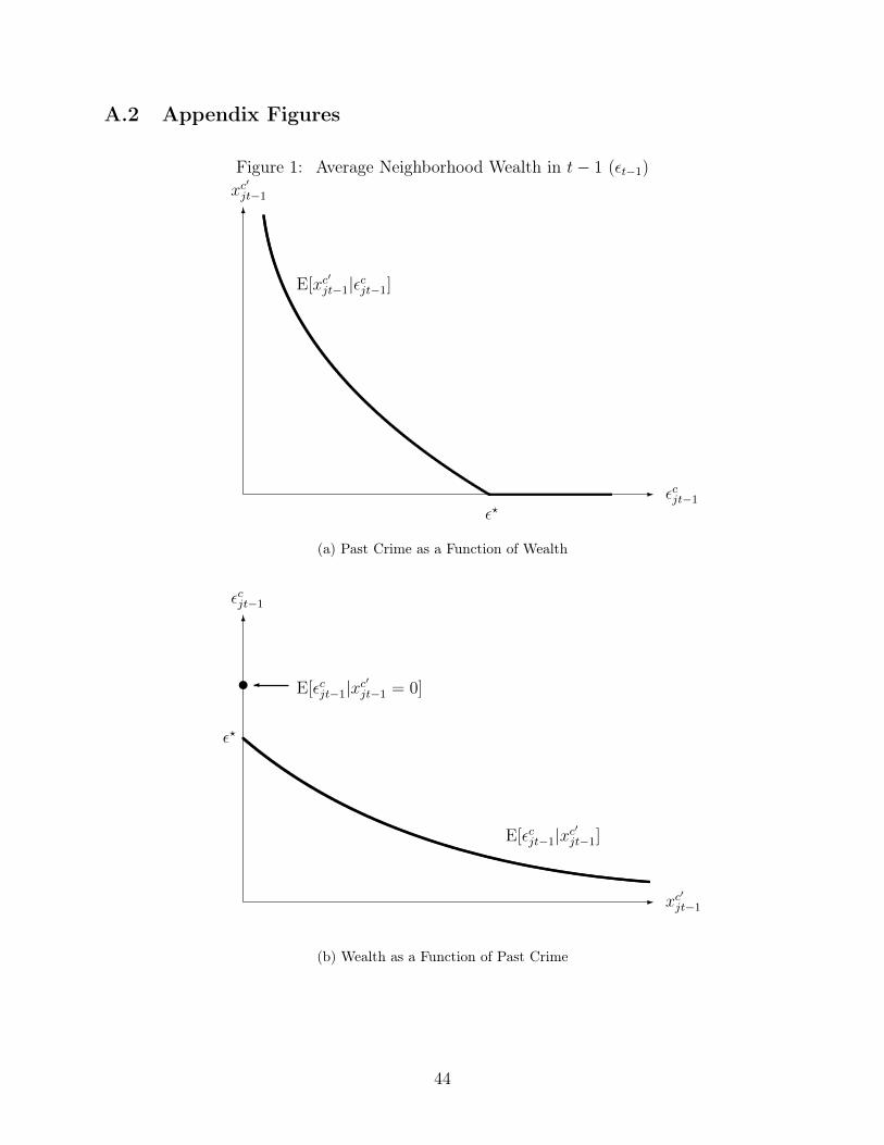
A.2 Appendix Figures

Figure 1: Average Neighborhood Wealth in t� 1 (✏t�1)

- ✏cjt�1

6

xc

0jt�1

E[xc

0jt�1|✏cjt�1]

✏?

(a) Past Crime as a Function of Wealth

- xc

0jt�1

6

✏cjt�1

E[✏cjt�1|xc

0jt�1]

u� E[✏cjt�1|xc

0jt�1 = 0]

✏?

(b) Wealth as a Function of Past Crime

44

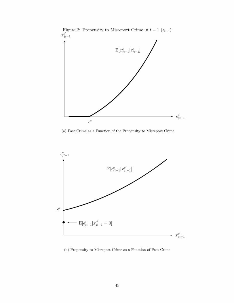
Figure 2: Propensity to Misreport Crime in t� 1 (✏t�1)

- ✏cjt�1

6

xc

0jt�1

E[xc

0jt�1|✏cjt�1]

✏?

(a) Past Crime as a Function of the Propensity to Misreport Crime

- xc

0jt�1

6

✏cjt�1

E[✏cjt�1|xc

0jt�1]

u � E[✏cjt�1|xc

0jt�1 = 0]

✏?

(b) Propensity to Misreport Crime as a Function of Past Crime

45

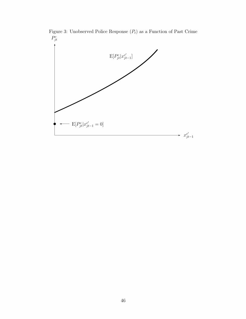
Figure 3: Unobserved Police Response (Pt

) as a Function of Past Crime

- xc

0jt�1

6

P c

jt

E[P c

jt

|xc

0jt�1]

u � E[P c

jt

|xc

0jt�1 = 0]

46

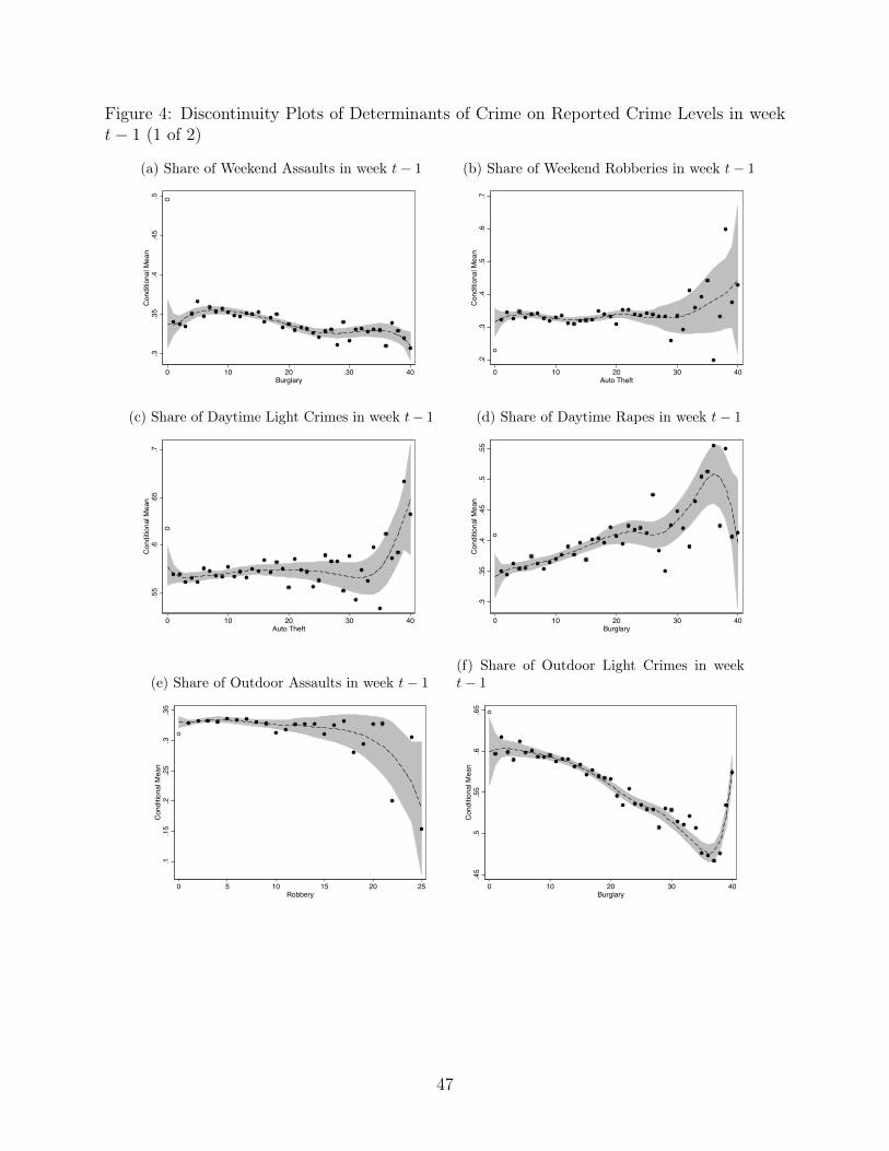
Figure 4: Discontinuity Plots of Determinants of Crime on Reported Crime Levels in weekt� 1 (1 of 2)

(a) Share of Weekend Assaults in week t� 1.3

.35

.4.4

5.5

Con

ditio

nal M

ean

0 10 20 30 40Burglary

(b) Share of Weekend Robberies in week t� 1

.2.3

.4.5

.6.7

Con

ditio

nal M

ean

0 10 20 30 40Auto Theft

(c) Share of Daytime Light Crimes in week t� 1

.55

.6.6

5.7

Con

ditio

nal M

ean

0 10 20 30 40Auto Theft

(d) Share of Daytime Rapes in week t� 1

.3.3

5.4

.45

.5.5

5C

ondi

tiona

l Mea

n

0 10 20 30 40Burglary

(e) Share of Outdoor Assaults in week t� 1

.1.1

5.2

.25

.3.3

5C

ondi

tiona

l Mea

n

0 5 10 15 20 25Robbery

(f) Share of Outdoor Light Crimes in weekt� 1

.45

.5.5

5.6

.65

Con

ditio

nal M

ean

0 10 20 30 40Burglary

47

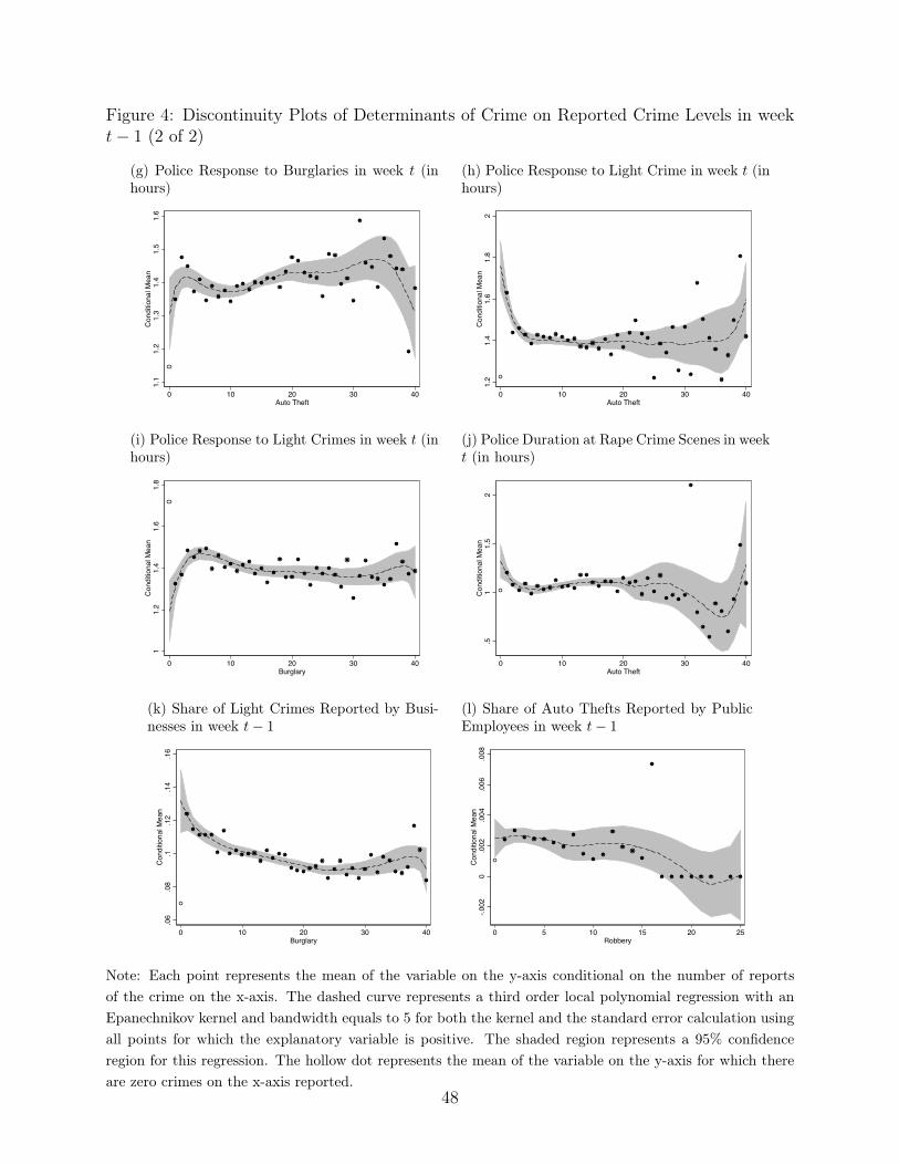
Figure 4: Discontinuity Plots of Determinants of Crime on Reported Crime Levels in weekt� 1 (2 of 2)

(g) Police Response to Burglaries in week t (inhours)

1.1

1.2

1.3

1.4

1.5

1.6

Con

ditio

nal M

ean

0 10 20 30 40Auto Theft

(h) Police Response to Light Crime in week t (inhours)

1.2

1.4

1.6

1.8

2C

ondi

tiona

l Mea

n

0 10 20 30 40Auto Theft

(i) Police Response to Light Crimes in week t (inhours)

11.

21.

41.

61.

8C

ondi

tiona

l Mea

n

0 10 20 30 40Burglary

(j) Police Duration at Rape Crime Scenes in weekt (in hours)

.51

1.5

2C

ondi

tiona

l Mea

n

0 10 20 30 40Auto Theft

(k) Share of Light Crimes Reported by Busi-nesses in week t� 1

.06

.08

.1.1

2.1

4.1

6C

ondi

tiona

l Mea

n

0 10 20 30 40Burglary

(l) Share of Auto Thefts Reported by PublicEmployees in week t� 1

-.002

0.0

02.0

04.0

06.0

08C

ondi

tiona

l Mea

n

0 5 10 15 20 25Robbery

Note: Each point represents the mean of the variable on the y-axis conditional on the number of reportsof the crime on the x-axis. The dashed curve represents a third order local polynomial regression with anEpanechnikov kernel and bandwidth equals to 5 for both the kernel and the standard error calculation usingall points for which the explanatory variable is positive. The shaded region represents a 95% confidenceregion for this regression. The hollow dot represents the mean of the variable on the y-axis for which thereare zero crimes on the x-axis reported.

48

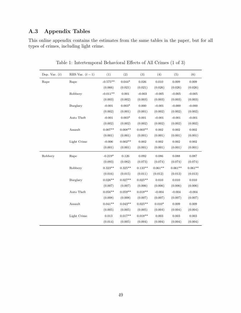
A.3 Appendix Tables

This online appendix contains the estimates from the same tables in the paper, but for alltypes of crimes, including light crime.

Table 1: Intertemporal Behavioral Effects of All Crimes (1 of 3)

Dep. Var. (t) RHS Var. (t� 1) (1) (2) (3) (4) (5) (6)

Rape Rape -0.575**

(0.066)

0.044*

(0.021)

0.026

(0.021)

0.010

(0.026)

0.009

(0.026)

0.009

(0.026)

Robbery -0.011**

(0.003)

0.001

(0.002)

-0.003

(0.003)

-0.005

(0.003)

-0.005

(0.003)

-0.005

(0.003)

Burglary -0.001

(0.002)

0.003*

(0.001)

0.000

(0.001)

-0.001

(0.002)

-0.000

(0.002)

-0.000

(0.002)

Auto Theft -0.001

(0.002)

0.003*

(0.002)

0.001

(0.002)

-0.001

(0.002)

-0.001

(0.002)

-0.001

(0.002)

Assault 0.007**

(0.001)

0.008**

(0.001)

0.003**

(0.001)

0.002

(0.001)

0.002

(0.001)

0.002

(0.001)

Light Crime -0.006

(0.001)

0.002**

(0.001)

0.002

(0.001)

0.002

(0.001)

0.002

(0.001)

0.002

(0.001)

Robbery Rape -0.219*

(0.093)

0.126

(0.082)

0.092

(0.073)

0.086

(0.074)

0.088

(0.074)

0.087

(0.074)

Robbery 0.323**

(0.016)

0.325**

(0.015)

0.133**

(0.011)

0.061**

(0.012)

0.061**

(0.013)

0.061**

(0.013)

Burglary 0.026**

(0.007)

0.027**

(0.007)

0.025**

(0.006)

0.010

(0.006)

0.010

(0.006)

0.010

(0.006)

Auto Theft 0.056**

(0.008)

0.059**

(0.008)

0.018**

(0.007)

-0.004

(0.007)

-0.004

(0.007)

-0.004

(0.007)

Assault 0.041**

(0.005)

0.043**

(0.005)

0.025**

(0.005)

0.010*

(0.004)

0.009

(0.004)

0.009

(0.004)

Light Crime 0.013

(0.014)

0.017**

(0.005)

0.018**

(0.004)

0.003

(0.004)

0.003

(0.004)

0.003

(0.004)

49

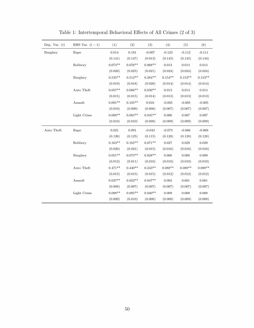
Table 1: Intertemporal Behavioral Effects of All Crimes (2 of 3)

Dep. Var. (t) RHS Var. (t� 1) (1) (2) (3) (4) (5) (6)

Burglary Rape 0.014

(0.141)

0.181

(0.147)

-0.007

(0.013)

-0.123

(0.145)

-0.112

(0.145)

-0.111

(0.144)

Robbery 0.074**

(0.026)

0.076**

(0.025)

0.068**

(0.021)

0.013

(0.024)

0.014

(0.024)

0.014

(0.024)

Burglary 0.535**

(0.019)

0.512**

(0.018)

0.284**

(0.020)

0.154**

(0.014)

0.153**

(0.014)

0.153**

(0.014)

Auto Theft 0.057**

(0.015)

0.086**

(0.015)

0.030**

(0.014)

0.013

(0.013)

0.014

(0.013)

0.014

(0.013)

Assault 0.091**

(0.010)

0.105**

(0.009)

0.016

(0.008)

-0.005

(0.007)

-0.005

(0.007)

-0.005

(0.007)

Light Crime 0.088**

(0.010)

0.085**

(0.010)

0.045**

(0.008)

0.006

(0.009)

0.007

(0.009)

0.007

(0.009)

Auto Theft Rape 0.021

(0.126)

0.091

(0.125)

-0.043

(0.115)

-0.073

(0.128)

-0.066

(0.128)

-0.069

(0.128)

Robbery 0.163**

(0.020)

0.165**

(0.021)

0.071**

(0.015)

0.027

(0.016)

0.029

(0.016)

0.029

(0.016)

Burglary 0.051**

(0.012)

0.075**

(0.011)

0.028**

(0.010)

0.008

(0.010)

0.008

(0.010)

0.009

(0.010)

Auto Theft 0.471**

(0.015)

0.440**

(0.015)

0.243**

(0.015)

0.088**

(0.012)

0.088**

(0.012)

0.088**

(0.012)

Assault 0.037**

(0.008)

0.022**

(0.007)

0.047**

(0.007)

0.002

(0.007)

0.001

(0.007)

0.001

(0.007)

Light Crime 0.088**

(0.009)

0.095**

(0.010)

0.040**

(0.008)

0.009

(0.008)

0.008

(0.009)

0.008

(0.008)

50

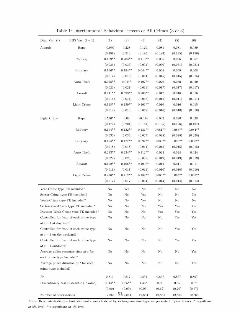
Table 1: Intertemporal Behavioral Effects of All Crimes (3 of 3)

Dep. Var. (t) RHS Var. (t� 1) (1) (2) (3) (4) (5) (6)

Assault Rape -0.030

(0.181)

0.228

(0.216)

0.129

(0.195)

0.081

(0.194)

0.081

(0.195)

0.089

(0.196)

Robbery 0.189**

(0.035)

0.203**

(0.033)

0.115**

(0.031)

0.056

(0.030)

0.056

(0.031)

0.057

(0.031)

Burglary 0.166**

(0.017)

0.194**

(0.015)

0.044**

(0.014)

0.009

(0.015)

0.009

(0.015)

0.008

(0.015)

Auto Theft 0.075**

(0.020)

0.043*

(0.021)

0.107**

(0.019)

0.029

(0.017)

0.030

(0.017)

0.029

(0.017)

Assault 0.611**

(0.016)

0.593**

(0.014)

0.206**

(0.016)

0.017

(0.012)

0.016

(0.011)

0.016

(0.011)

Light Crime 0.148**

(0.012)

0.159**

(0.013)

0.101**

(0.012)

0.016

(0.010)

0.016

(0.010)

0.015

(0.010)

Light Crime Rape 1.536**

(0.172)

0.09

(0.201)

-0.034

(0.181)

0.032

(0.195)

0.020

(0.196)

0.028

(0.197)

Robbery 0.164**

(0.033)

0.132**

(0.034)

0.131**

(0.027)

0.081**

(0.028)

0.083**

(0.028)

0.084**

(0.028)

Burglary 0.194**

(0.018)

0.177**

(0.018)

0.097**

(0.014)

0.038**

(0.015)

0.038**

(0.015)

0.038**

(0.015)

Auto Theft 0.233**

(0.022)

0.234**

(0.023)

0.112**

(0.019)

0.024

(0.019)

0.024

(0.019)

0.024

(0.019)

Assault 0.162**

(0.011)

0.166**

(0.011)

0.103**

(0.011)

0.012

(0.010)

0.011

(0.010)

0.011

(0.010)

Light Crime 0.436**

(0.017)

0.412**

(0.017)

0.182**

(0.014)

0.066**

(0.014)

0.065**

(0.014)

0.065**

(0.014)

Year-Crime type FE included? No Yes No No No No

Sector-Crime type FE included? No No Yes No No No

Week-Crime type FE included? No No Yes No No No

Sector-Year-Crime type FE included? No No No Yes Yes Yes

Division-Week-Crime type FE included? No No No Yes Yes Yes

Controlled for frac. of each crime type

at t� 1 at daytime?

No No No No Yes Yes

Controlled for frac. of each crime type

at t� 1 on the weekend?

No No No No Yes Yes

Controlled for frac. of each crime type

at t� 1 outdoors?

No No No No Yes Yes

Average police response time at t for

each crime type included?

No No No No No Yes

Average police duration at t for each

crime type included?

No No No No No Yes

R

2 0.810 0.812 0.851 0.867 0.867 0.867

Discontinuity test F-statistic (P value) 11.14**

(0.00)

1.85**

(0.00)

1.46*

(0.05)

0.90

(0.62)

0.85

(0.70)

0.87

(0.67)

Number of observations 12,864 12,864 12,864 12,864 12,864 12,864

Notes: Heteroskedasticity robust standard errors clustered by sector-year-crime type are presented in parentheses. *: significant

at 5% level. **: significant at 1% level.

51

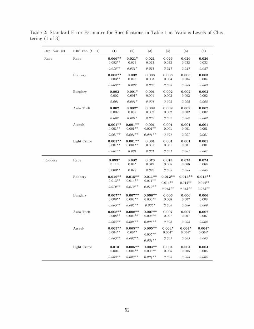
Table 2: Standard Error Estimates for Specifications in Table 1 at Various Levels of Clus-tering (1 of 3)

Dep. Var. (t) RHS Var. (t� 1) (1) (2) (3) (4) (5) (6)

Rape Rape 0.066**

0.082**

0.048**

0.021*

0.023

0.021*

0.021

0.023

0.021

0.026

0.032

0.027

0.026

0.032

0.027

0.026

0.032

0.027

Robbery 0.003**

0.003**

0.003**

0.002

0.003

0.002

0.003

0.003

0.003

0.003

0.004

0.003

0.003

0.004

0.003

0.003

0.004

0.003

Burglary 0.002

0.002

0.001

0.001*

0.001*

0.001*

0.001

0.001

0.001

0.002

0.002

0.002

0.002

0.002

0.002

0.002

0.002

0.002

Auto Theft 0.002

0.002

0.002

0.002*

0.002

0.001*

0.002

0.002

0.002

0.002

0.002

0.002

0.002

0.002

0.002

0.002

0.002

0.002

Assault 0.001**

0.001**

0.001**

0.001**

0.001**

0.001**

0.001

0.001**

0.001**

0.001

0.001

0.001

0.001

0.001

0.001

0.001

0.001

0.001

Light Crime 0.001**

0.001**

0.001**

0.001**

0.001**

0.001

0.001

0.001

0.001

0.001

0.001

0.001

0.001

0.001

0.001

0.001

0.001

0.001

Robbery Rape 0.093*

0.113

0.069**

0.082

0.06*

0.079

0.073

0.049

0.073

0.074

0.065

0.085

0.074

0.066

0.085

0.074

0.066

0.085

Robbery 0.016**

0.013**

0.010**

0.015**

0.014**

0.010**

0.011**

0.011**

0.010**

0.012**

0.014**

0.013**

0.013**

0.014**

0.013**

0.013**

0.014**

0.013**

Burglary 0.007**

0.008**

0.005**

0.007**

0.008**

0.005**

0.006**

0.006**

0.005*

0.006

0.008

0.006

0.006

0.007

0.006

0.006

0.008

0.006

Auto Theft 0.008**

0.008**

0.005**

0.008**

0.009**

0.006**

0.007**

0.006**

0.006**

0.007

0.007

0.008

0.007

0.007

0.008

0.007

0.007

0.008

Assault 0.005**

0.004**

0.003**

0.005**

0.00**

0.003**

0.005**

0.005**

0.004**

0.004*

0.004*

0.005

0.004*

0.004*

0.005

0.004*

0.004*

0.005

Light Crime 0.013

0.004

0.003**

0.005**

0.004**

0.003**

0.004**

0.005**

0.004**

0.004

0.005

0.005

0.004

0.005

0.005

0.004

0.005

0.005

52

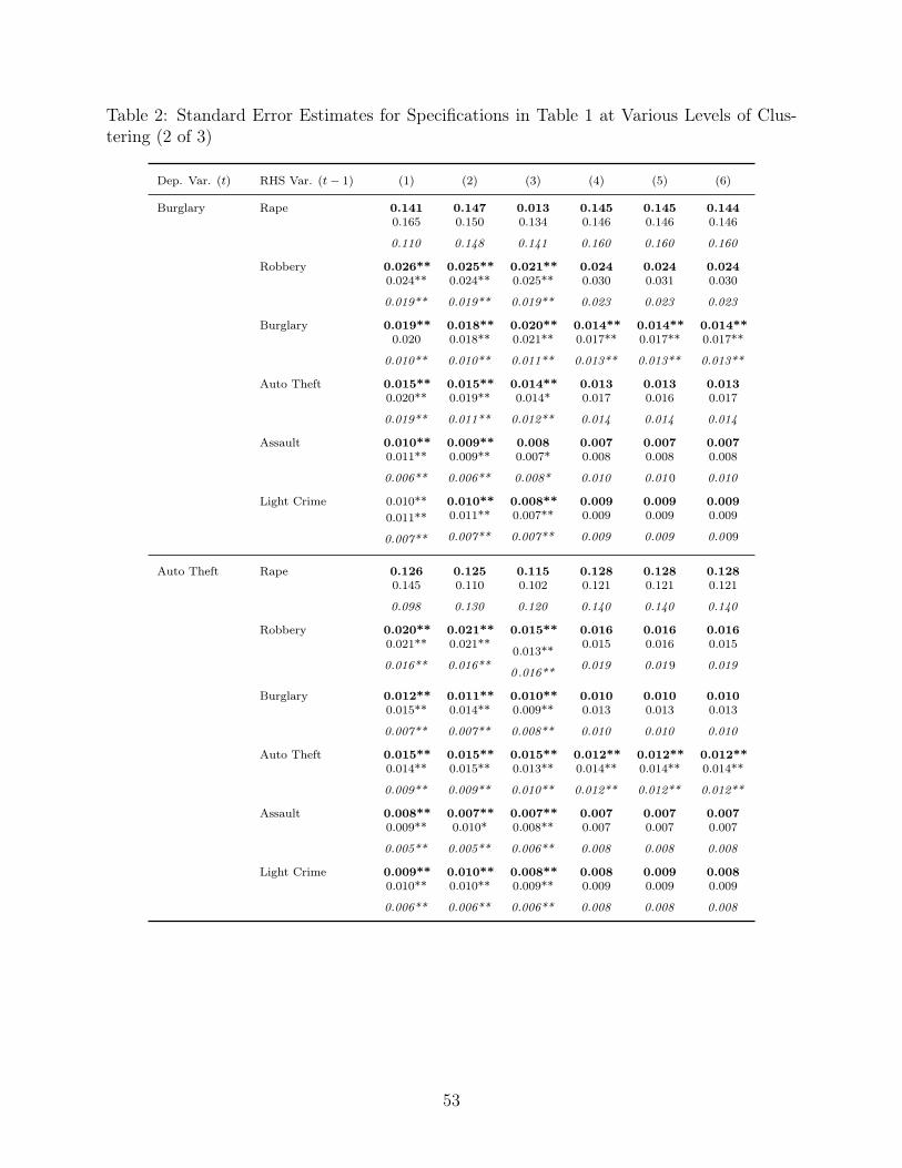
Table 2: Standard Error Estimates for Specifications in Table 1 at Various Levels of Clus-tering (2 of 3)

Dep. Var. (t) RHS Var. (t� 1) (1) (2) (3) (4) (5) (6)

Burglary Rape 0.141

0.165

0.110

0.147

0.150

0.148

0.013

0.134

0.141

0.145

0.146

0.160

0.145

0.146

0.160

0.144

0.146

0.160

Robbery 0.026**

0.024**

0.019**

0.025**

0.024**

0.019**

0.021**

0.025**

0.019**

0.024

0.030

0.023

0.024

0.031

0.023

0.024

0.030

0.023

Burglary 0.019**

0.020

0.010**

0.018**

0.018**

0.010**

0.020**

0.021**

0.011**

0.014**

0.017**

0.013**

0.014**

0.017**

0.013**

0.014**

0.017**

0.013**

Auto Theft 0.015**

0.020**

0.019**

0.015**

0.019**

0.011**

0.014**

0.014*

0.012**

0.013

0.017

0.014

0.013

0.016

0.014

0.013

0.017

0.014

Assault 0.010**

0.011**

0.006**

0.009**

0.009**

0.006**

0.008

0.007*

0.008*

0.007

0.008

0.010

0.007

0.008

0.010

0.007

0.008

0.010

Light Crime 0.010**0.011**

0.007**

0.010**

0.011**

0.007**

0.008**

0.007**

0.007**

0.009

0.009

0.009

0.009

0.009

0.009

0.009

0.009

0.009

Auto Theft Rape 0.126

0.145

0.098

0.125

0.110

0.130

0.115

0.102

0.120

0.128

0.121

0.140

0.128

0.121

0.140

0.128

0.121

0.140

Robbery 0.020**

0.021**

0.016**

0.021**

0.021**

0.016**

0.015**

0.013**

0 .016**

0.016

0.015

0.019

0.016

0.016

0.019

0.016

0.015

0.019

Burglary 0.012**

0.015**

0.007**

0.011**

0.014**

0.007**

0.010**

0.009**

0.008**

0.010

0.013

0.010

0.010

0.013

0.010

0.010

0.013

0.010

Auto Theft 0.015**

0.014**

0.009**

0.015**

0.015**

0.009**

0.015**

0.013**

0.010**

0.012**

0.014**

0.012**

0.012**

0.014**

0.012**

0.012**

0.014**

0.012**

Assault 0.008**

0.009**

0.005**

0.007**

0.010*

0.005**

0.007**

0.008**

0.006**

0.007

0.007

0.008

0.007

0.007

0.008

0.007

0.007

0.008

Light Crime 0.009**

0.010**

0.006**

0.010**

0.010**

0.006**

0.008**

0.009**

0.006**

0.008

0.009

0.008

0.009

0.009

0.008

0.008

0.009

0.008

53

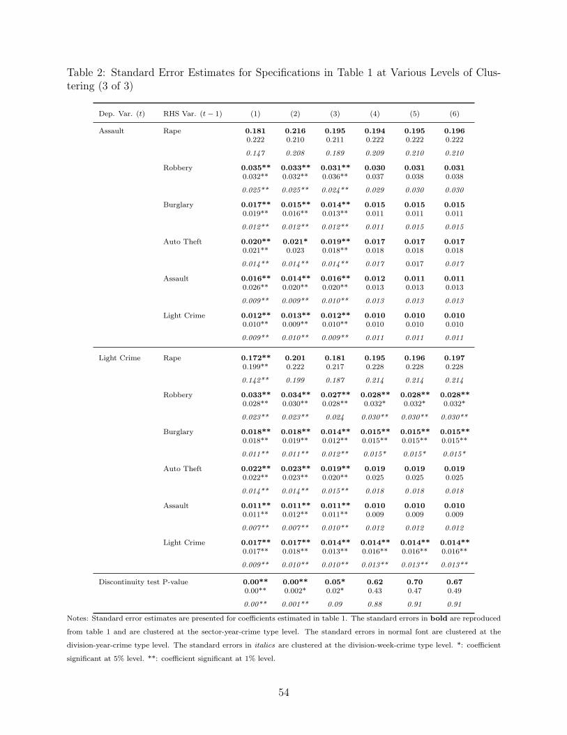
Table 2: Standard Error Estimates for Specifications in Table 1 at Various Levels of Clus-tering (3 of 3)

Dep. Var. (t) RHS Var. (t� 1) (1) (2) (3) (4) (5) (6)

Assault Rape 0.181

0.222

0.147

0.216

0.210

0.208

0.195

0.211

0.189

0.194

0.222

0.209

0.195

0.222

0.210

0.196

0.222

0.210

Robbery 0.035**

0.032**

0.025**

0.033**

0.032**

0.025**

0.031**

0.036**

0.024**

0.030

0.037

0.029

0.031

0.038

0.030

0.031

0.038

0.030

Burglary 0.017**

0.019**

0.012**

0.015**

0.016**

0.012**

0.014**

0.013**

0.012**

0.015

0.011

0.011

0.015

0.011

0.015

0.015

0.011

0.015

Auto Theft 0.020**

0.021**

0.014**

0.021*

0.023

0.014**

0.019**

0.018**

0.014**

0.017

0.018

0.017

0.017

0.018

0.017

0.017

0.018

0.017

Assault 0.016**

0.026**

0.009**

0.014**

0.020**

0.009**

0.016**

0.020**

0.010**

0.012

0.013

0.013

0.011

0.013

0.013

0.011

0.013

0.013

Light Crime 0.012**

0.010**

0.009**

0.013**

0.009**

0.010**

0.012**

0.010**

0.009**

0.010

0.010

0.011

0.010

0.010

0.011

0.010

0.010

0.011

Light Crime Rape 0.172**

0.199**

0.142**

0.201

0.222

0.199

0.181

0.217

0.187

0.195

0.228

0.214

0.196

0.228

0.214

0.197

0.228

0.214

Robbery 0.033**

0.028**

0.023**

0.034**

0.030**

0.023**

0.027**

0.028**

0.024

0.028**

0.032*

0.030**

0.028**

0.032*

0.030**

0.028**

0.032*

0.030**

Burglary 0.018**

0.018**

0.011**

0.018**

0.019**

0.011**

0.014**

0.012**

0.012**

0.015**

0.015**

0.015*

0.015**

0.015**

0.015*

0.015**

0.015**

0.015*

Auto Theft 0.022**

0.022**

0.014**

0.023**

0.023**

0.014**

0.019**

0.020**

0.015**

0.019

0.025

0.018

0.019

0.025

0 .018

0.019

0.025

0.018

Assault 0.011**

0.011**

0.007**

0.011**

0.012**

0.007**

0.011**

0.011**

0.010**

0.010

0.009

0.012

0.010

0.009

0.012

0.010

0.009

0.012

Light Crime 0.017**

0.017**

0.009**

0.017**

0.018**

0.010**

0.014**

0.013**

0.010**

0.014**

0.016**

0.013**

0.014**

0.016**

0.013**

0.014**

0.016**

0.013**

Discontinuity test P-value 0.00**

0.00**

0.00**

0.00**

0.002*

0.001**

0.05*

0.02*

0.09

0.62

0.43

0.88

0.70

0.47

0.91

0.67

0.49

0.91

Notes: Standard error estimates are presented for coefficients estimated in table 1. The standard errors in bold are reproduced

from table 1 and are clustered at the sector-year-crime type level. The standard errors in normal font are clustered at the

division-year-crime type level. The standard errors in italics are clustered at the division-week-crime type level. *: coefficient

significant at 5% level. **: coefficient significant at 1% level.

54

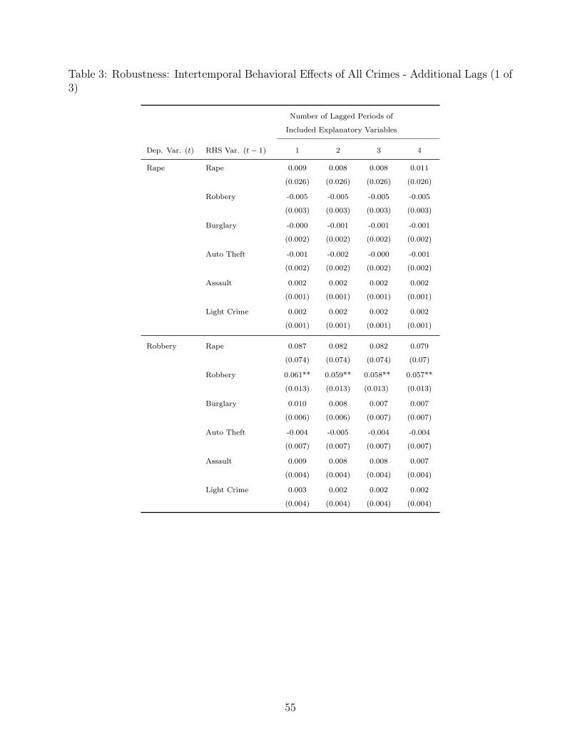
Table 3: Robustness: Intertemporal Behavioral Effects of All Crimes - Additional Lags (1 of3)

Number of Lagged Periods of

Included Explanatory Variables

Dep. Var. (t) RHS Var. (t� 1) 1 2 3 4

Rape Rape 0.009

(0.026)

0.008

(0.026)

0.008

(0.026)

0.011

(0.026)

Robbery -0.005

(0.003)

-0.005

(0.003)

-0.005

(0.003)

-0.005

(0.003)

Burglary -0.000

(0.002)

-0.001

(0.002)

-0.001

(0.002)

-0.001

(0.002)

Auto Theft -0.001

(0.002)

-0.002

(0.002)

-0.000

(0.002)

-0.001

(0.002)

Assault 0.002

(0.001)

0.002

(0.001)

0.002

(0.001)

0.002

(0.001)

Light Crime 0.002

(0.001)

0.002

(0.001)

0.002

(0.001)

0.002

(0.001)

Robbery Rape 0.087

(0.074)

0.082

(0.074)

0.082

(0.074)

0.079

(0.07)

Robbery 0.061**

(0.013)

0.059**

(0.013)

0.058**

(0.013)

0.057**

(0.013)

Burglary 0.010

(0.006)

0.008

(0.006)

0.007

(0.007)

0.007

(0.007)

Auto Theft -0.004

(0.007)

-0.005

(0.007)

-0.004

(0.007)

-0.004

(0.007)

Assault 0.009

(0.004)

0.008

(0.004)

0.008

(0.004)

0.007

(0.004)

Light Crime 0.003

(0.004)

0.002

(0.004)

0.002

(0.004)

0.002

(0.004)

55

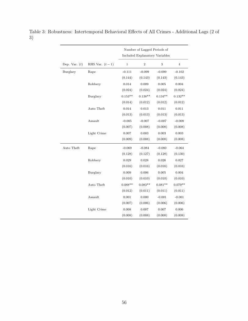
Table 3: Robustness: Intertemporal Behavioral Effects of All Crimes - Additional Lags (2 of3)

Number of Lagged Periods of

Included Explanatory Variables

Dep. Var. (t) RHS Var. (t� 1) 1 2 3 4

Burglary Rape -0.111

(0.144)

-0.099

(0.143)

-0.099

(0.143)

-0.102

(0.143)

Robbery 0.014

(0.024)

0.009

(0.024)

0.005

(0.024)

0.004

(0.024)

Burglary 0.153**

(0.014)

0.138**

(0.012)

0.134**

(0.012)

0.132**

(0.012)

Auto Theft 0.014

(0.013)

0.013

(0.013)

0.011

(0.013)

0.011

(0.013)

Assault -0.005

(0.007)

-0.007

(0.008)

-0.007

(0.008)

-0.008

(0.008)

Light Crime 0.007

(0.009)

0.003

(0.008)

0.003

(0.008)

0.003

(0.008)

Auto Theft Rape -0.069

(0.128)

-0.084

(0.127)

-0.080

(0.128)

-0.064

(0.130)

Robbery 0.029

(0.016)

0.028

(0.016)

0.026

(0.016)

0.027

(0.016)

Burglary 0.009

(0.010)

0.006

(0.010)

0.005

(0.010)

0.004

(0.010)

Auto Theft 0.088**

(0.012)

0.083**

(0.011)

0.081**

(0.011)

0.079**

(0.011)

Assault 0.001

(0.007)

0.000

(0.006)

-0.001

(0.006)

-0.001

(0.006)

Light Crime 0.008

(0.008)

0.007

(0.008)

0.007

(0.008)

0.006

(0.008)

56

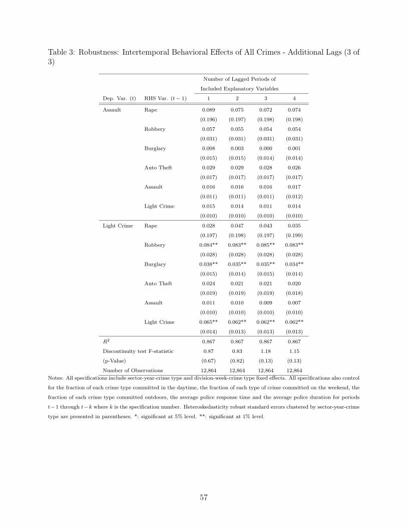
Table 3: Robustness: Intertemporal Behavioral Effects of All Crimes - Additional Lags (3 of3)

Number of Lagged Periods of

Included Explanatory Variables

Dep. Var. (t) RHS Var. (t� 1) 1 2 3 4

Assault Rape 0.089

(0.196)

0.075

(0.197)

0.072

(0.198)

0.074

(0.198)

Robbery 0.057

(0.031)

0.055

(0.031)

0.054

(0.031)

0.054

(0.031)

Burglary 0.008

(0.015)

0.003

(0.015)

0.000

(0.014)

0.001

(0.014)

Auto Theft 0.029

(0.017)

0.029

(0.017)

0.028

(0.017)

0.026

(0.017)

Assault 0.016

(0.011)

0.016

(0.011)

0.016

(0.011)

0.017

(0.012)

Light Crime 0.015

(0.010)

0.014

(0.010)

0.011

(0.010)

0.014

(0.010)

Light Crime Rape 0.028

(0.197)

0.047

(0.198)

0.043

(0.197)

0.035

(0.199)

Robbery 0.084**

(0.028)

0.083**

(0.028)

0.085**

(0.028)

0.083**

(0.028)

Burglary 0.038**

(0.015)

0.035**

(0.014)

0.035**

(0.015)

0.034**

(0.014)

Auto Theft 0.024

(0.019)

0.021

(0.019)

0.021

(0.019)

0.020

(0.018)

Assault 0.011

(0.010)

0.010

(0.010)

0.009

(0.010)

0.007

(0.010)

Light Crime 0.065**

(0.014)

0.062**

(0.013)

0.062**

(0.013)

0.062**

(0.013)

R

2 0.867 0.867 0.867 0.867

Discontinuity test F-statistic

(p-Value)

0.87

(0.67)

0.83

(0.82)

1.18

(0.13)

1.15

(0.13)

Number of Observations 12,864 12,864 12,864 12,864Notes: All specifications include sector-year-crime type and division-week-crime type fixed effects. All specifications also control

for the fraction of each crime type committed in the daytime, the fraction of each type of crime committed on the weekend, the

fraction of each crime type committed outdoors, the average police response time and the average police duration for periods

t�1 through t�k where k is the specification number. Heteroskedasticity robust standard errors clustered by sector-year-crime

type are presented in parentheses. *: significant at 5% level. **: significant at 1% level.

57

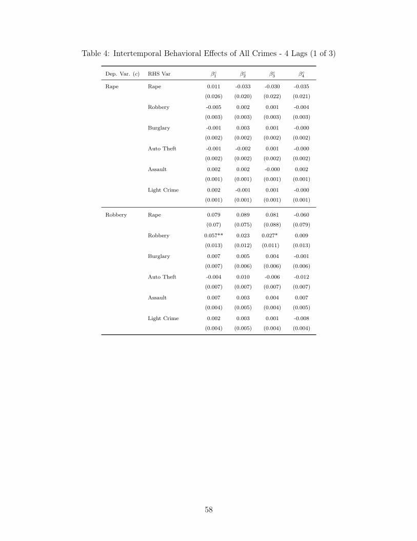
Table 4: Intertemporal Behavioral Effects of All Crimes - 4 Lags (1 of 3)

Dep. Var. (c) RHS Var �

c1 �

c2 �

c3 �

c4

Rape Rape 0.011

(0.026)

-0.033

(0.020)

-0.030

(0.022)

-0.035

(0.021)

Robbery -0.005

(0.003)

0.002

(0.003)

0.001

(0.003)

-0.004

(0.003)

Burglary -0.001

(0.002)

0.003

(0.002)

0.001

(0.002)

-0.000

(0.002)

Auto Theft -0.001

(0.002)

-0.002

(0.002)

0.001

(0.002)

-0.000

(0.002)

Assault 0.002

(0.001)

0.002

(0.001)

-0.000

(0.001)

0.002

(0.001)

Light Crime 0.002

(0.001)

-0.001

(0.001)

0.001

(0.001)

-0.000

(0.001)

Robbery Rape 0.079

(0.07)

0.089

(0.075)

0.081

(0.088)

-0.060

(0.079)

Robbery 0.057**

(0.013)

0.023

(0.012)

0.027*

(0.011)

0.009

(0.013)

Burglary 0.007

(0.007)

0.005

(0.006)

0.004

(0.006)

-0.001

(0.006)

Auto Theft -0.004

(0.007)

0.010

(0.007)

-0.006

(0.007)

-0.012

(0.007)

Assault 0.007

(0.004)

0.003

(0.005)

0.004

(0.004)

0.007

(0.005)

Light Crime 0.002

(0.004)

0.003

(0.005)

0.001

(0.004)

-0.008

(0.004)

58

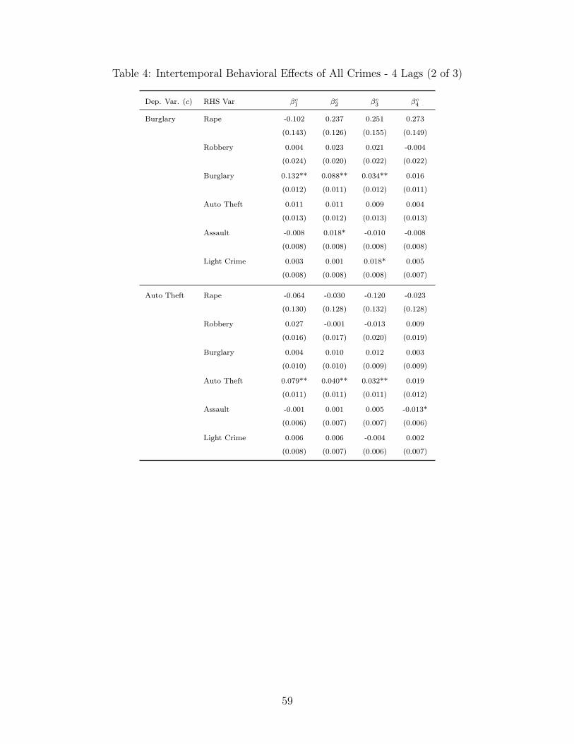
Table 4: Intertemporal Behavioral Effects of All Crimes - 4 Lags (2 of 3)

Dep. Var. (c) RHS Var �

c1 �

c2 �

c3 �

c4

Burglary Rape -0.102

(0.143)

0.237

(0.126)

0.251

(0.155)

0.273

(0.149)

Robbery 0.004

(0.024)

0.023

(0.020)

0.021

(0.022)

-0.004

(0.022)

Burglary 0.132**

(0.012)

0.088**

(0.011)

0.034**

(0.012)

0.016

(0.011)

Auto Theft 0.011

(0.013)

0.011

(0.012)

0.009

(0.013)

0.004

(0.013)

Assault -0.008

(0.008)

0.018*

(0.008)

-0.010

(0.008)

-0.008

(0.008)

Light Crime 0.003

(0.008)

0.001

(0.008)

0.018*

(0.008)

0.005

(0.007)

Auto Theft Rape -0.064

(0.130)

-0.030

(0.128)

-0.120

(0.132)

-0.023

(0.128)

Robbery 0.027

(0.016)

-0.001

(0.017)

-0.013

(0.020)

0.009

(0.019)

Burglary 0.004

(0.010)

0.010

(0.010)

0.012

(0.009)

0.003

(0.009)

Auto Theft 0.079**

(0.011)

0.040**

(0.011)

0.032**

(0.011)

0.019

(0.012)

Assault -0.001

(0.006)

0.001

(0.007)

0.005

(0.007)

-0.013*

(0.006)

Light Crime 0.006

(0.008)

0.006

(0.007)

-0.004

(0.006)

0.002

(0.007)

59

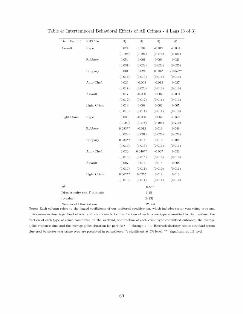
Table 4: Intertemporal Behavioral Effects of All Crimes - 4 Lags (3 of 3)

Dep. Var. (c) RHS Var. �

c1 �

c2 �

c3 �

c4

Assault Rape 0.074

(0.198)

0.134

(0.194)

-0.019

(0.170)

-0.081

(0.181)

Robbery 0.054

(0.031)

0.001

(0.028)

0.003

(0.024)

0.021

(0.025)

Burglary 0.001

(0.014)

0.024

(0.013)

0.036*

(0.015)

-0.052**

(0.014)

Auto Theft 0.026

(0.017)

-0.003

(0.020)

-0.013

(0.016)

0.027

(0.016)

Assault 0.017

(0.012)

-0.000

(0.012)

0.002

(0.011)

-0.001

(0.013)

Light Crime 0.014

(0.010)

0.008

(0.011)

0.002

(0.011)

0.005

(0.010)

Light Crime Rape 0.035

(0.199)

-0.060

(0.178)

0.082

(0.194)

-0.327

(0.210)

Robbery 0.083**

(0.028)

-0.012

(0.031)

0.016

(0.026)

0.046

(0.028)

Burglary 0.034**

(0.014)

0.014

(0.015)

0.010

(0.015)

-0.010

(0.015)

Auto Theft 0.020

(0.018)

0.040**

(0.015)

-0.007

(0.016)

0.023

(0.019)

Assault 0.007

(0.010)

0.014

(0.011)

0.014

(0.010)

0.008

(0.011)

Light Crime 0.062**

(0.013)

0.025*

(0.011)

0.018

(0.011)

0.013

(0.012)

R

2 0.867

Discontinuity test F-statistic

(p-value)

1.15

(0.13)

Number of Observations 12,864Notes: Each column refers to the lagged coefficients of our preferred specification, which includes sector-year-crime type and

division-week-crime type fixed effects, and also controls for the fraction of each crime type committed in the daytime, the

fraction of each type of crime committed on the weekend, the fraction of each crime type committed outdoors, the average

police response time and the average police duration for periods t� 1 through t� 4. Heteroskedasticity robust standard errors

clustered by sector-year-crime type are presented in parentheses. *: significant at 5% level. **: significant at 1% level.

60