DMSHP Evaluation Report 12-30-2016 (without track changes)ma-eeac.org/wordpress/wp-content/uploads/Ductless-Mini-Split-Heat... · Unit Efficiency COP ... Table 14. Energy Savings,

Ductless Mini‐Split Heat

Pump Impact Evaluation December 30, 2016

Prepared for:

The Electric and Gas Program Administrators of Massachusetts and Rhode Island

Part of the Residential Evaluation Program Area

This page left blank.

Prepared by:

Dave Korn, PE, CEM

John Walczyk, CEM

Ari Jackson

Andrew Machado, PE, CEM

John Kongoletos, CEM

Eric Pfann

The Cadmus Group, Inc.

This page left blank.

i

Table of Contents Executive Summary ....................................................................................................................................... 1

Research Objectives ............................................................................................................................... 1

Sample Design .................................................................................................................................. 1

Findings ................................................................................................................................................... 4

Analysis Notes .................................................................................................................................. 4

Operating Hours ............................................................................................................................... 5

Equivalent Full Load Hours .............................................................................................................. 5

Savings ............................................................................................................................................. 8

Cold Climate Performance ............................................................................................................. 15

Discussion ............................................................................................................................................. 20

Cooling ........................................................................................................................................... 20

Heating ........................................................................................................................................... 21

COP/SEER/HSPF ............................................................................................................................. 21

Savings Values ................................................................................................................................ 22

Controls and Zoning ....................................................................................................................... 23

Recommendations................................................................................................................................ 23

Program ......................................................................................................................................... 23

Future Studies ................................................................................................................................ 24

Introduction ................................................................................................................................................ 26

Program and Evaluation ....................................................................................................................... 27

Research Objectives ............................................................................................................................. 27

Existing Research .................................................................................................................................. 28

Method ....................................................................................................................................................... 30

Sample Design ...................................................................................................................................... 30

Engineering Background ....................................................................................................................... 32

Efficiency Metrics ........................................................................................................................... 32

Seasonal Efficiency Metrics ............................................................................................................ 34

Energy ............................................................................................................................................ 36

Airflow ............................................................................................................................................ 38

Data Collection ..................................................................................................................................... 38

ii

Power ............................................................................................................................................. 38

Fan Current .................................................................................................................................... 39

Airflow ............................................................................................................................................ 40

Temperature and Relative Humidity ............................................................................................. 41

Heating Systems ............................................................................................................................. 43

Site Attributes ................................................................................................................................ 45

Analysis ................................................................................................................................................. 46

Airflow ............................................................................................................................................ 46

Weather Normalization ................................................................................................................. 46

Climate During the Study ............................................................................................................... 47

Manual J: Residential Load Calculation ......................................................................................... 49

Savings ........................................................................................................................................... 50

Results ......................................................................................................................................................... 54

Load Shapes .......................................................................................................................................... 54

Operating Hours ................................................................................................................................... 60

Equivalent Full Load Hours ................................................................................................................... 61

Performance ......................................................................................................................................... 73

Unit Efficiency COP ............................................................................................................................... 86

Cold Climate Performance ............................................................................................................. 87

Multi‐Head Performance ............................................................................................................... 89

Performance Related to Installing Contractors ............................................................................. 91

Heating System Interaction .................................................................................................................. 93

Unit Sizing ............................................................................................................................................. 95

Behavior Influence .............................................................................................................................. 101

Additional Findings ............................................................................................................................. 102

Filter Cleanliness .......................................................................................................................... 102

Outdoor Unit Placement .............................................................................................................. 103

Indoor Unit Placement ................................................................................................................. 107

Unit Controls ................................................................................................................................ 108

Staging of Alternative Heating Systems ....................................................................................... 109

Localized Heating ......................................................................................................................... 115

iii

Non‐Energy Benefits .................................................................................................................... 115

Discussion ................................................................................................................................................. 117

Cooling ................................................................................................................................................ 117

Heating ............................................................................................................................................... 118

COP/SEER/HSPF .................................................................................................................................. 118

Savings Values .................................................................................................................................... 119

Controls and Zoning ........................................................................................................................... 120

Airflow ................................................................................................................................................ 120

Recommendations .................................................................................................................................... 122

Recommendations.............................................................................................................................. 122

Program ....................................................................................................................................... 122

Future Studies .............................................................................................................................. 123

Appendix A: Measuring Airflow in DMSHPs.............................................................................................. 124

Appendix B: Baseline Memorandum Chart .............................................................................................. 142

Appendix C: TRM Memorandum, December 2, 2016 ............................................................................... 143

Appendix D: Example DMSHP Time Series Data ....................................................................................... 147

iv

Table of Figures Figure ES‐1. Locations of Sampled Residences ............................................................................................. 3

Figure ES‐2.DMSHP EFLH vs. Season* ........................................................................................................... 7

Figure ES‐3. DMSHP Usage vs. Purchase Intent and Season ........................................................................ 8

Figure ES‐4. Average Heating COP vs. Outdoor Air Temperature for Cold‐Climate and Non‐Cold‐Climate

Systems—Winter 2015 ............................................................................................................................... 16

Figure ES‐5. Average Heating COP vs. Outdoor Air Temperature for Cold‐Climate and Non‐Cold‐Climate

Systems—Winter 2016 ............................................................................................................................... 16

Figure ES‐6. Operational Break Point Temperature of Heating with DMSHP, Winter 2016, All Units ....... 18

Figure ES‐7. Operational Break Point Temperature of Heating with DMSHP, Winter 2016, Cold Climate

Units ............................................................................................................................................................ 19

Figure 1. DMSHP Outdoor Unit ................................................................................................................... 26

Figure 2. DMSHP Indoor Unit ...................................................................................................................... 26

Figure 3. Locations of Sampled Residences ................................................................................................ 31

Figure 4. Indoor Unit Mass Flow ................................................................................................................. 37

Figure 5. Power Metering Setup Installed on an Outdoor Unit .................................................................. 39

Figure 6. Current Transformers Installed on Fan Wires .............................................................................. 40

Figure 7. Balometer ..................................................................................................................................... 41

Figure 8. Outdoor Entering Air Temperature and Relative Humidity Sensor ............................................. 42

Figure 9. Leaving Air Sensors on a DMSHP Head ........................................................................................ 43

Figure 10. Entering Air Sensors on a DMSHP Head..................................................................................... 43

Figure 11. Boiler System Monitoring .......................................................................................................... 44

Figure 12. Furnace System Monitoring ....................................................................................................... 45

Figure 13. Cumulative Distribution of Winter Hours Versus Temperature Bin .......................................... 48

Figure 14. Cumulative Distribution of Summer Hours Versus Temperature Bin ........................................ 49

Figure 15. Winter 2015 Average Power Consumption vs. Time of Day, N=99 ........................................... 54

Figure 16. Summer 2015 Average Power Consumption vs. Time of Day, N=115 ....................................... 55

Figure 17. Winter 2016 Average Power Consumption vs. Time of Day, N=60 ........................................... 55

Figure 18. Winter 2015 Average Power Consumption While Heating vs. Outdoor Air Temperature ........ 56

Figure 19. Summer 2015 Average Power Consumption While Cooling vs. Outdoor Air Temperature,

N=114 .......................................................................................................................................................... 57

v

Figure 20. Winter 2016 Average Power Consumption While Heating vs. Outdoor Air Temperature, N=57

.................................................................................................................................................................... 57

Figure 21. Winter 2015 Average Power Consumption vs. Time, N=99 ....................................................... 58

Figure 22. Winter 2015 Average Power Consumption vs. Time, N=51, Cold Climate Units ....................... 58

Figure 23. Summer 2015 Average Power Consumption vs. Time, N=115 .................................................. 59

Figure 24. Winter 2016 Average Power Consumption vs. Time, N=60 ....................................................... 59

Figure 25. Winter 2016 Average Power Consumption vs. Time, N=35, Cold Climate Units ....................... 60

Figure 26. DMSHP EFLH vs. Season ............................................................................................................. 62

Figure 27. DMSHP EFLH vs. Season, Cold Climate Units ............................................................................. 63

Figure 28. DMSHP EFLH vs. Purchase Intent and Season ........................................................................... 64

Figure 29. DMSHP EFLH vs. Purchase Intent and Season, Cold Climate Units ............................................ 64

Figure 30. Measured Seasonal Efficiencies ................................................................................................. 74

Figure 31. Measured Seasonal Efficiencies, Cold Climate Units ................................................................. 74

Figure 32. Winter 2015 Measured HSPF vs. EFLH, N=86 ............................................................................ 75

Figure 33. Summer 2015 Measured SEER vs. EFLH, N=113 ........................................................................ 75

Figure 34. Winter 2016 Measured HSPF vs. EFLH, N=57 ............................................................................ 76

Figure 35. Winter 2015 HSPF vs. System Configuration, N=87 ................................................................... 77

Figure 36. Summer 2015 SEER vs. System Configuration, N=114 ............................................................... 77

Figure 37. Winter 2016 HSPF vs. System Configuration, N=57 ................................................................... 78

Figure 38. Winter 2015 HSPF vs. System Configuration and Usage, N=86 ................................................. 78

Figure 39. Summer 2015 SEER vs. System Configuration and Usage, N=113 ............................................. 79

Figure 40. Winter 2016 HSPF vs. System Configuration and Usage, N=57 ................................................. 79

Figure 41. Seasonal Efficiencies vs. Purchase Intent................................................................................... 80

Figure 42. Seasonal Efficiencies vs. Purchase Intent, Cold Climate Units ................................................... 80

Figure 43. Winter 2015 Maximum Observed Capacity vs. Rated Capacity, N=98 ...................................... 81

Figure 44. Summer 2015 Maximum Observed Capacity vs. Rated Capacity, N=114 .................................. 82

Figure 45. Winter 2016 Maximum Observed Capacity vs. Rated Capacity, N=60 ...................................... 82

Figure 46. Winter 2015 Rated HSPF vs. Rated Capacity, N=98 ................................................................... 83

Figure 47. Summer 2015 Rated SEER vs. Rated Capacity, N=114 ............................................................... 83

Figure 48. Winter 2016 Rated HSPF vs. Rated Capacity, N=60 ................................................................... 84

Figure 49. Winter 2015 Observed HSPF vs. Rated HSPF, N=86 .................................................................. 85

vi

Figure 50. Summer 2015 Observed SEER vs. Rated SEER, N=113 ............................................................... 85

Figure 51. Winter 2015 Observed HSPF vs. Rated HSPF, N=57 .................................................................. 85

Figure 52. Winter 2015 Average COP vs. Outdoor Air Temperature, N=87 ............................................... 86

Figure 53. Summer 2015 Average COP vs. Outdoor Air Temperature, N=114 ........................................... 87

Figure 54. Average Heating COP vs. Outdoor Air Temperature for Cold‐Climate and Non‐Cold‐Climate

Systems – Winter 2015 ............................................................................................................................... 88

Figure 55. Average Heating COP vs. Outdoor Air Temperature for Cold‐Climate and Non‐Cold‐Climate

Systems – Winter 2016 ............................................................................................................................... 89

Figure 56. Average Heating COP vs. Outdoor Air Temperature for One‐, Two‐, and Three‐Head Systems

.................................................................................................................................................................... 90

Figure 57. Average Heating COP vs. Outdoor Air Temperature for One‐, Two‐, and Three‐Head Non‐

Cold‐Climate Systems ................................................................................................................................. 91

Figure 58. Average Winter 2015 COP vs. Outdoor Air Temperature for Installing Contractor .................. 92

Figure 59. Average Winter 2016 COP vs. Outdoor Air Temperature for Installing Contractor .................. 92

Figure 60. Site M0193, Heating System Interaction ................................................................................... 93



Figure 63. Calculated Thermal Loads of Spaces Served by DMSHPs, N=141 .............................................. 96

Figure 64. Ratio of DMSHP Rated Capacity to Calculated Thermal Load of Spaces Served, N=140 ........... 96

Figure 65. Ratio of DMSHP Rated Capacity to Floor Area of Spaces Served .............................................. 97

Figure 66. Heating and Cooling Rated Capacities Normalized by Calculated Design Loads ....................... 98

Figure 67. Relationship Between Design Cooling, Design Heating, and Rated Capacities as a Function of

Floor Area Served ........................................................................................................................................ 99

Figure 68. Normalized HVAC System Capacities ....................................................................................... 100

Figure 69. Behavior Influence Postcard .................................................................................................... 101

Figure 70. DMSHP Usage for Behavior Influence Postcard Recipients ..................................................... 102

Figure 71. Filter Maintenance ................................................................................................................... 103

Figure 72. Clearances Underneath Outdoor Units ................................................................................... 104

Figure 73. Clearances Around Outdoor Units ........................................................................................... 105

Figure 74. Maintaining Clearances in Wintertime .................................................................................... 106

Figure 75. DMSHPs in Windy Environment ............................................................................................... 107

Figure 76. Vertical Clearance on Indoor Unit ............................................................................................ 108

vii

Figure 77. Operation of DMSHP Remote Control ..................................................................................... 109

Figure 78. Operational Break Point Temperature of Heating with DMSHP, Winter 2016, All Units ........ 112

Figure 79. Operational Break Point Temperature of Heating with DMSHP, Winter 2016, Cold Climate

Units .......................................................................................................................................................... 113

Figure 80. Operational Break Point Temperature of Heating with DMSHP, Assumed HSPF of 13 ........... 114

Figure 81. LBNL‐5983E Figure 14 .............................................................................................................. 126

Figure 82. LBNL‐5983E Figure 14, Adapted .............................................................................................. 127

Figure 83. Inlet vs. Outlet Flow ................................................................................................................. 127

Figure 84. Proximity Sensor Arrangement (NREL Image 18330) .............................................................. 128

Figure 85. Optical Tachometer Data Collection ........................................................................................ 130

Figure 86. Basis of Experimental Powered Flow Hood Setup (Figure 4 from Williamson 2015) .............. 132

Figure 87. Convergence Nozzle: ASHRAE 51‐1999 Figure 5 (Excerpt) ...................................................... 133

Figure 88. Powered Flow Hood Testing Setup .......................................................................................... 133

Figure 89. Powered Flow Hood Testing Setup .......................................................................................... 134

Figure 90. Extended Testing Site B: Large‐Unit Powered Flow Hood ....................................................... 135

Figure 91. Indoor Head Prior to Testing .................................................................................................... 136

Figure 92. Non‐Powered Flow Hood (Balometer) Setup .......................................................................... 137

Figure 93. Non‐Powered Flow Hood (Balometer) Setup .......................................................................... 138

Figure 94. Vane Position: Powered Flow Hood ......................................................................................... 139

Figure 95. Coil State: Wet vs. Dry ............................................................................................................. 140

Figure 96. Powered Flow Hood Flow Restriction ...................................................................................... 141

viii

Table of Tables Table ES‐1. Program Populations Strata ....................................................................................................... 2

Table ES‐2. Average Nameplate Ratings for Outdoor Units ......................................................................... 4

Table ES‐3. Observed Run Hours for Nominal Heating and Cooling Seasons* ............................................. 5

Table ES‐4.Average EFLH ............................................................................................................................... 6

Table ES‐5. Energy Savings by Season and Baseline System ......................................................................... 9

Table ES‐6. Demand Savings by Season and Baseline System .................................................................... 10

Table ES‐7. Energy Savings, Each Baseline Applied to All Sites, Top 25% ................................................... 11

Table ES‐8. Peak Demand Savings, Baseline Applied Based on Survey Responses and Existing Systems,

Top 25% ...................................................................................................................................................... 12

Table ES‐9. Weighted Average Savings, Fuel Switching .............................................................................. 13

Table ES‐10. Weighted Average Savings, Non‐Fuel Switching .................................................................... 14

Table 1. Program Populations ..................................................................................................................... 27

Table 2. Comparison of Previous Research ................................................................................................. 29

Table 3. Program Populations Strata .......................................................................................................... 31

Table 4. Average Ratings for Measured Outdoor Units .............................................................................. 32

Table 5. Observed Weather During the Study ............................................................................................ 47

Table 6. Savings Calculation Methodology for Alternative Heating/Cooling Equipment ........................... 53

Table 7. CFs for Peak Winter and Summer Periods .................................................................................... 60

Table 8. Observed Run Hours for Nominal Heating and Cooling Seasons* ................................................ 61

Table 9. Average EFLH ................................................................................................................................. 62

Table 10. Energy Savings, Each Baseline Applied to All Sites ...................................................................... 65

Table 11. Peak Demand Savings, Each Baseline Applied to All Sites .......................................................... 66

Table 12. Energy Savings, Baseline Applied Based on Survey Responses and Existing Systems ................ 67

Table 13. Peak Demand Savings, Baseline Applied Based on Survey Responses and Existing Systems ..... 67

Table 14. Energy Savings, Each Baseline Applied to All Sites, Top 25% ...................................................... 69

Table 15. Peak Demand Savings, Each Baseline Applied to All Sites, Top 25% .......................................... 69

Table 16. Weighted Average Savings, Fuel Switching ................................................................................. 71

Table 17. Weighted Average Savings, Non‐Fuel Switching ......................................................................... 72

Table 18. Cold‐Climate Unit Listing ............................................................................................................. 87

ix

Table 19. Heating and Cooling Capacities, N=137 ...................................................................................... 98

Table 20. Savings for Residential DMSHPs ................................................................................................ 144

Table 21. Heating and Cooling Equivalent Full Load Hours for DMSHP.................................................... 144

Table 22. Recommended DMSHP Baselines ............................................................................................. 145

1

Executive Summary

The Massachusetts and Rhode Island Program Administrators (PAs) commissioned Cadmus and its

subcontractors, Navigant and Tetra Tech, (the evaluation team) to conduct an in situ evaluation of

ductless mini‐split heat pumps (DMSHPs). The evaluation team initially planned to study 132

Massachusetts homes that participated in the COOL SMART Program. The PAs, however, extended the

scope of work to include 20 Rhode Island homes that participated in the High Efficiency Heating and

Cooling Rebate Program.

Research Objectives The evaluation sought to address many utility and consumer questions about DMSHPs, focusing on

power and energy consumption, heat output, efficiency, and interactions with existing HVAC equipment.

The specific research questions follow:

How much energy is being saved with the average installation of a DMSHP through the

programs?

What are the relevant baseline equipment configurations and associated energy consumptions

and load shapes?

During each season, when are DMSHPs operating, how much energy are they consuming, and

how much heating and cooling are they providing?

How does DMSHP performance correlate with rated capacity, rated efficiency, and ambient

conditions?

How do cold‐climate DMSHPs and standard unit performances compare?

How does unit sizing affect heating performance?

How do DMSHPs interact with central heating systems?

What factors limit the use and performance of DMSHPs?

Are program contractors sizing DMSHPs properly?

Sample Design

The evaluation team used the following participant parameters to stratify program populations into

key groups:

Cold‐climate or non‐cold‐climate unit sites1

1 DMSHP manufacturers offer units that claim high performance at very cold (below 0 °F) outdoor ambient

temperatures. The evaluation team used the Efficiency Vermont Technical Reference Manual that was current

during the study’s planning phase to identify cold‐climate units. As the report shows, units not characterized

as cold climate can operate at 0 °F, although there are not the same claims of high performance at very cold

temperatures.

2

Single‐ or multi‐head unit sites2

Installed by the largest vendor or by all other contractors

In collaboration with evaluation stakeholders, the team identified these parameters at the study’s

outset, and then used them to inform sample targets during the participant recruiting process. Initially,

the team designed the sampling based on Massachusetts’ 2012–2013 program population, but later

expanded this to include Massachusetts’ 2014 program population and Rhode Island’s 2013 program

population. Massachusetts participants from the 2014 program year did not receive online surveys (i.e.,

the study added them after the surveys had been completed). In 2015, a separate Rhode Island survey

examined the similarity between Massachusetts and Rhode Island populations. This sought to justify the

application of the study results to the Rhode Island population. Sample sizes were determined by the

PAs and the evaluation team with a target of 90/20 confidence and precision for each stratum, assuming

a coefficient of variation of 0.7. Table ES‐1 details these program populations, as measured by

participant surveys, program tracking data, and collected evaluation data.

Table ES‐1. Program Populations Strata

Sites

MA 2012–

2013 Program

Participant

Share

MA 2014

Program

Participant

Share

RI 2013

Program

Participant

Share

Study

Sample

Participant

Share

Study Sample

Participant

Planned

Target

Study

Sample

Participant

Count

Cold‐climate unit sites(1) 41% 15% 22% 51% 34 78

Non‐cold‐climate unit sites 59% 85% 78% 49% 34 74

Single‐head unit sites 48% Unknown(2) 73% 50% 34 107

Multiple‐head unit sites 52% Unknown 27% 50% 34 45

Installed by largest (MA)

vendor sites 13% 7% 0% 28% 34 43

Installed by all other vendor

sites 87% 93% 100% 72% 34 109

Population Total 3,229 1,055 507 n/a n/a n/a

Sample Total(3) 112 20 20 n/a 135 152(1)All cold‐climate unit sites contained single‐head units only. (2)Because 2014 Massachusetts participants were not surveyed, these data were not readily available for the total program population.

(3)Many categories overlap, producing a strata total greater than the overall totals.

2 A DMSHP consist of an outdoor unit that serves one or more indoor heads that deliver heating and cooling.

Single‐head units have one such head; multi‐head units have more than one head.

3

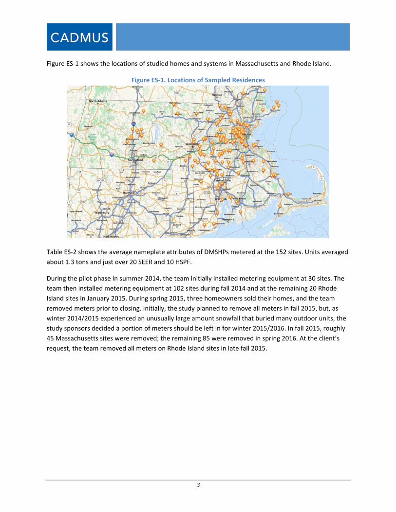
Figure ES‐1 shows the locations of studied homes and systems in Massachusetts and Rhode Island.

Figure ES‐1. Locations of Sampled Residences

Table ES‐2 shows the average nameplate attributes of DMSHPs metered at the 152 sites. Units averaged

about 1.3 tons and just over 20 SEER and 10 HSPF.

During the pilot phase in summer 2014, the team initially installed metering equipment at 30 sites. The

team then installed metering equipment at 102 sites during fall 2014 and at the remaining 20 Rhode

Island sites in January 2015. During spring 2015, three homeowners sold their homes, and the team

removed meters prior to closing. Initially, the study planned to remove all meters in fall 2015, but, as

winter 2014/2015 experienced an unusually large amount snowfall that buried many outdoor units, the

study sponsors decided a portion of meters should be left in for winter 2015/2016. In fall 2015, roughly

45 Massachusetts sites were removed; the remaining 85 were removed in spring 2016. At the client’s

request, the team removed all meters on Rhode Island sites in late fall 2015.

4

Table ES‐2. Average Nameplate Ratings for Outdoor Units

System

Category

Sample

Size

Average Rated

Cooling Capacity

(nominal cooling

at 95°F)(1)

[Btu/h]

Average

Rated

Heating

Capacity at

47°F

[Btu/h]

Average

Rated

Heating

Capacity at

17°F

[Btu/h]

Average

Rated

EER(2)

[Btu/Wh]

Average

Rated

SEER(3)

[Btu/Wh]

Average

Rated

HSPF(4)

[Btu/Wh]

All 152 16,435 19,491 11,426 13.2 20.6 10.3

Cold Climate

Units (CC) 78 14,680 17,985 10,409 13.8 22.3 11.0

Non CC, multi 45 20,444 23,484 13,682 12.4 17.9 9.2

Non CC single 29 14,414 17,268 10,632 12.7 20.3 10.2(1)Capacity is measured per Air‐Conditioning, Heating, and Refrigeration Institute (AHRI) guidelines for various outdoor temperatures: 95 °F, 47 °F, and 17 °F.

(2)Energy Efficiency Ratio (EER) equals the cooling heating provided (in BTUs), divided by the power consumption in watts—essentially the coefficient of performance (COP) times 3.412. It is tested at an outdoor temperature of 95°F and an indoor temperature of 80°F.

(3)Seasonal Energy Efficiency Ratio (SEER) equals the cooling heating provided (in BTUs), divided by the power consumption in watts—essentially the coefficient of performance (COP) times 3.412. It is tested at outside air temperatures ranging from 67°F to 95°F, with the lower temperatures weighted more heavily, and is meant to represent seasonal performance. The indoor temperature is set to 80°F.

(4)Heating Seasonal Performance Factor (HSPF) equals the heating provided (in BTUs), divided by the power consumption in watts—essentially the COP times 3.412. It is tested at outside air temperatures ranging from 17°F to 62°F, and represents seasonal performance. The indoor temperature is set to 70°F.

Findings

Analysis Notes

This report uses many box and whisker plot graphs. The boxes show a range of data from the 25th to the

75th percentile, otherwise known as the 1rst and 3rd quartiles. The middle line in each box is the median

data point, or the 50th percentile. Half of the data lie above this line and half fall below. The lines

extending above and below the boxes represent the upper 25% and lowest 25% of the

data, respectively.

The evaluation team based all energy‐use calculations on “site” energy, meaning the calculations did not

include line losses and energy‐generation losses. Compared energy costs—energy costs at the site or

meter—represent the amount paid by the consumer.

In all, the study metered 152 homes. Of these, nearly all power meter files were sufficiently complete

for a basic analysis. This study’s analyses were based on continual logging of BTUs and COP. To meter

this effectively, meter sets had to concurrently log total power, fan amperage, supply temperature and

relative humidity (RH), and return temperature and RH. If these parameters were not metered for a

period, BTUs could not be calculated for that period. Consequently, sample sizes (n) shown in the graphs

were lower than 152. Similarly, 85 sites metered for winter 2015/2016 resulted in sample sizes lower

5

than 85 for the second consecutive winter. Nevertheless, as this study represents the largest DMSHP

study completed to date, the net sample sizes provide a broad and detailed view of DMSHP operations.

We present results for two winters: 2015 where near historically deep snowfalls buried many units for

up to 1 month and 2016 which was warmer and had little snow. Because the units were buried and not

fully functional for 2015 and because this is not likely to re‐occur, we recommend using the winter 2016

results. Both winter’s results are shown throughout the report.

Operating Hours

Table ES‐3 shows simple run‐time hours for metered DMSHPs, with a unit logged as running if its power

draw exceeded a threshold standby power of 60W. Looking at the nominal heating season, the average

unit ran about 27% of the time (793 hours) during 2015, and about 24% of the time (703 hours) during

2016. Note that an operating hour differs from a full‐load hour in that an operating hour simply means

that the unit remained on at some capacity, whereas a full‐load hour indicates the unit ran at full

capacity.

Table ES‐3. Observed Run Hours for Nominal Heating and Cooling Seasons*

Season Example Period of

Operation

Season

(Days)

Season

(Hours)

Mean Percent

Runtime

Operation

Hours

Winter 2015 December‐March 121 2,904 27.3% 793

Summer 2015 June‐August 92 2,208 19.4% 428


*These observed run times address periods where the unit drew more than 60W (non‐standby).

Equivalent Full Load Hours

Table ES‐4 shows the average equivalent full load hours (EFLH) across all units for two heating seasons

and one cooling season studied, comparing these values with those prescribed in the Massachusetts and

Rhode Island Technical Reference Manuals (TRMs) and the averages of the top 25% of sites in the study.

Values for the two heating seasons (442 and 451) remained consistent with the value (447) presented in

this study’s October 12, 2015, Heating Memorandum, but differed from the current 1,200 TRM value.

The summer value (218) was roughly 15% lower than the value shown in the Cooling Memorandum3

(distributed in February 2016 and finalized (259) on May 2, 2016), and differed from the 360 TRM value.

This reduction in average cooling EFLH resulted from this report’s use of site‐specific, typical

meteorological year (TMY) data, in contrast to statewide TMY data used in the memo, as well as the

evaluation team filtering out energy usage that consumed power but did not provide cooling. The right

most column of Table ES‐4 shows the average EFLH of the units in the top 25th percentile. These values

are at or above the TRM values.

3 Cadmus Group. Ductless Mini‐Split Heat Pump Draft Cooling Season Results. January 22, 2016.

6

Table ES‐4. Average EFLH

Season 2013–2015

MA TRM

2014 RI

TRM

Average

Study EFLH

Average of Top 25% of

Measured EFLH

Winter 2015 1,200 1,200 442 1,275

Summer 2015 360 360 218 499

Winter 2016 1,200 1,200 451 1,117

This study produced EFLH lower than values indicated in the applicable Massachusetts and Rhode Island

TRMs for conventional heating and cooling systems (e.g., gas‐fired furnaces, central air conditioning).

These variances occurred for the following reasons:

Not all units were used routinely for each season. Many units were lightly used (or not used at

all) for heating or cooling. Figure ES‐2 illustrates this behavior, with the bottom of the box

indicating the 25th percentile of the hour range at or very near zero for winter 2015.

Many units remained off during the summer’s cooler periods.

Some units in heating mode operated coincidently with primary systems (many of which were

fossil fuel‐based).

Systems were sized larger than the cooling needs of the immediate spaces they served, as

discussed later in the report.

The units operated at some level for 19% to 27% of the time for the two winter and one summer

season, and were off or on standby for much of the time (Table ES‐2). Comparing the EFLH to

the total operating hours one can see that the units operate on average at about 56% and 64%

of capacity for winter 2015 and winter 2016 and at about 51% of capacity for the summer.

TRM sources for legacy EFLH values could be inappropriate for DMSHPs. The cooling EFLH value

(360) was based on a 2009 study of central air conditioners. The heating EFLH value (1,200) was

sourced from a “Massachusetts Common Assumption” also used for other types of heating

equipment. Both legacy values appear high relative to this study’s findings, supporting the

theory that homeowners used DMSHPs differently than conventional heating or

cooling equipment.

The average ELFH of the top 25th percentile of units have values close to or above the TRM

values.

7

Figure ES‐2. DMSHP EFLH vs. Season*

*The blue boxes delineate first and third data quartiles. The lines (whiskers) indicate upper and

lower quartiles. The plus symbols represent outliers (points greater than or less than 1.5*(Inter

Quartile Range), where the IQR equals the distance between the first and third quartiles).

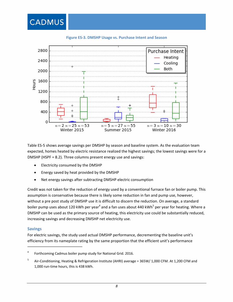
Figure ES‐3 more closely examines this variation, showing that units bought for “both heating and

cooling” were used much more for heating than units where users identified their purchases as for

“cooling only.” Winter 2016 was a milder than winter 2015, and units operated more efficiently during

the former season, resulting in lower EFLH for users intending “both heating and cooling.” During winter

2016, units purchased for “cooling only” saw some heating usage.

8

Figure ES‐3. DMSHP Usage vs. Purchase Intent and Season

Table ES‐5 shows average savings per DMSHP by season and baseline system. As the evaluation team

expected, homes heated by electric resistance realized the highest savings; the lowest savings were for a

DMSHP (HSPF = 8.2). Three columns present energy use and savings:

Electricity consumed by the DMSHP

Energy saved by heat provided by the DMSHP

Net energy savings after subtracting DMSHP electric consumption

Credit was not taken for the reduction of energy used by a conventional furnace fan or boiler pump. This

assumption is conservative because there is likely some reduction in fan and pump use, however,

without a pre post study of DMSHP use it is difficult to discern the reduction. On average, a standard

boiler pump uses about 120 kWh per year4 and a fan uses about 440 kWh5 per year for heating. Where a

DMSHP can be used as the primary source of heating, this electricity use could be substantially reduced,

increasing savings and decreasing DMSHP net electricity use.

Savings

For electric savings, the study used actual DMSHP performance, decrementing the baseline unit’s

efficiency from its nameplate rating by the same proportion that the efficient unit’s performance

4 Forthcoming Cadmus boiler pump study for National Grid. 2016.

5 Air‐Conditioning, Heating & Refrigeration Institute (AHRI) average = 365W/ 1,000 CFM. At 1,200 CFM and

1,000 run‐time hours, this is 438 kWh.

9

differed from its rating. Cooling savings increased with lower efficiency baselines. Savings calculations

relative to a central air conditioner baseline included a 15% duct loss,6 decreasing the central unit’s net

efficiency. Table ES‐6 shows demand savings.

Table ES‐5. Energy Savings by Season and Baseline System

Season Baseline System Sample

Size

Electric Usage

of DMSHP

[kWh]

Baseline

Energy

Reduction

Net Energy

Savings

Precision at 90%

Confidence [%]

Winter

2015

90% AFUE Furnace(1)

98

683 4.87 MMBtu 2.54 MMBtu 37

85% AFUE Furnace(2) 683 5.16 MMBtu 2.83 MMBtu 36

82% AFUE Boiler 683 4.54 MMBtu 2.21 MMBtu 39

HSPF 7.7 DMSHP 683 907 kWh 224 kWh 21


Electric Resistance 683 1,092 kWh 409 kWh 48

Summer

2015

EER 9.8 Window AC

114

159 213 kWh 54 kWh 15

SEER 13.0 Central AC 159 288 kWh 129 kWh 14

SEER 13.0 DMSHP 159 245 kWh 86 kWh 14


Winter

2016

90% AFUE Furnace

60

763 6.9 MMBtu 4.3 MMBtu 37

85% AFUE Furnace 763 7.31 MMBtu 4.7 MMBtu 36




Electric Resistance 763 1,547 kWh 784 kWh 42(1) Duct losses assumed at 15%. (2) Baseline efficiency prescribed by relevant Massachusetts (2013‐2015) and Rhode Island (2015) TRMs in force when the study began.

6 Massachusetts Technical Reference Manual, 2013–2015 Program Years, HVAC‐Duct Sealing, assumed

baseline efficiency.

10

Table ES‐6. Demand Savings by Season and Baseline System


Size

Electric

Usage of

DMSHP

[kW]

Baseline

Power

Reduction

[kW]

Average Peak

Period

Demand

Savings [kW]

Precision at

90%

Confidence

[%]

Winter

2015

90% AFUE Furnace

98

0.21 0 ‐0.21 33

85% AFUE Furnace 0.21 0 ‐0.21 33

82% AFUE Boiler 0.21 0 ‐0.21 33

HSPF 7.7 DMSHP 0.21 0.28 0.07 22

HSPF 8.2 DMSHP 0.21 0.26 0.05 22

Electric Resistance 0.21 0.33 0.12 43

Summer

2015

EER 9.8 Window AC

114

0.11 0.15 0.04 16

SEER 13.0 Central AC 0.11 0.20 0.09 15

SEER 13.0 DMSHP 0.11 0.05 0.06 15

SEER 14.5 DMSHP 0.11 0.07 0.04 15

Winter

2016

90% AFUE Furnace

60

0.25 0 ‐0.25 34

85% AFUE Furnace 0.25 0 ‐0.25 34

82% AFUE Boiler 0.25 0 ‐0.25 34

HSPF 7.7 DMSHP 0.25 0.33 0.08 24

HSPF 8.2 DMSHP 0.25 0.31 0.06 25


To examine the practical potential savings achievable by DMSHPs used more frequently, the evaluation

team took sites in the top 25%, based on savings. Table ES‐7 and Table ES‐8 show savings for this

subpopulation. Usage and savings were much higher than the mean, as one would expect

mathematically. In practical terms, these were savings expected upon removing units lightly used or not

used from the population.

11

Table ES‐7. Energy Savings, Each Baseline Applied to All Sites, Top 25%

Season Baseline

System Sample Size

Electric

Usage of

DMSHP

[kWh]

Baseline

Energy

Reduction

Average Energy

Savings

Precision at

90%

Confidence

[%]

Winter 2015

90% AFUE

Furnace

25

1,414 14.7 MMBtu 9.84 MMBtu 22

85% AFUE

Furnace 1,414 15.5 MMBtu 10.70 MMBtu 22

82% AFUE

Boiler 1,414 13.1 MMBtu 8.86 MMBtu 22

HSPF 7.7

DMSHP 1,894 2,536 kWh 642 kWh 10

HSPF 8.2

DMSHP 1,894 2,382 kWh 488 kWh 11

Electric

Resistance 1,414 3,287 kWh 1,873 kWh 24

Summer

2015

EER 9.8

Window AC

29

358 484 kWh 126 kWh 12

SEER 13.0

Central AC 371 663 kWh 292 kWh 11

SEER 13.0

DMSHP 363 556 kWh 193 kWh 12

SEER 14.5

DMSHP 332 468 kWh 136 kWh 14

Winter 2016

90% AFUE

Furnace

15

1,56618.68

MMBtu13.34 MMBtu 30

85% AFUE

Furnace 1,566

19.78

MMBtu14.44 MMBtu 30

82% AFUE

Boiler 1,566

17.43

MMBtu12.09 MMBtu 31

HSPF 7.7

DMSHP 1,862 2,433 kWh 571 kWh 13

HSPF 8.2

DMSHP 1,761 2,184 kWh 423 kWh 15

Electric

Resistance 1,566 4,188 2,622 kWh 33

Similarly, Table ES‐8 shows demand savings for the top 25% of sites.

12

Table ES‐8. Peak Demand Savings, Baseline Applied Based on Survey Responses and Existing Systems, Top 25%

Season Baseline System Sample Size

Electric

Usage of

DMSHP [kW]

Baseline

Power

Reduction

[kW]

Average Peak

Period

Demand

Savings [kW]

Precision at

90%

Confidence

[%]

Winter

2015

90% AFUE

Furnace

25

0.47 0 ‐0.47 18

85% AFUE

Furnace 0.47 0 ‐0.47 18

82% AFUE Boiler 0.47 0 ‐0.47 18

HSPF 7.7

DMSHP 0.62 0.82 0.20 13

HSPF 8.2

DMSHP 0.56 0.70 0.14 14

Electric

Resistance 0.47 1.02 0.55 19

Summer

2015

EER 9.8 Window

AC

29

0.24 0.33 0.09 13

SEER 13.0

Central AC 0.25 0.45 0.20 11

SEER 13.0

DMSHP 0.23 0.36 0.13 12

SEER 14.5

DMSHP 0.22 0.31 0.09 13

Winter

2016

90% AFUE

Furnace

15

0.54 0 ‐0.54 25

85% AFUE

Furnace 0.54 0 ‐0.54 25

82% AFUE Boiler 0.54 0 ‐0.54 25

HSPF 7.7

DMSHP 0.61 0.80 0.19 12

HSPF 8.2

DMSHP 0.61 0.76 0.15 15

Electric

Resistance 0.54 1.64 1.1 26

13

Using baseline weighting from the previously published Baseline Memorandum, the evaluation team calculated average weighted savings for each of the three

studied seasons, both for a single and specific baseline, as shown in Table ES‐9. The terms “Single Baseline” and “Specific Baseline” differentiate the

methodologies used in calculating savings; the former averages DMSHP usage across all participants and applies various baselines to the result, and the latter

calculates savings using survey responses indicating participant specific baselines. Generally, winter 2016, with data unaffected by the large snowfalls of 2015,

realized higher savings. Specific baselines showed savings similar to, or somewhat higher than, single baselines, but at poorer (higher) precisions.

Table ES‐9. Weighted Average Savings, Fuel Switching

Fuel Switching Single Baseline Specific Baseline

Season

Baseline

System

Base

Eff.

Efficiency

Metric

Savings

Units n

Mean

Savings

Mean

Savings

[kWh]

Population

with

Baseline

[%]

Expected

Baseline

Savings

[kWh]

Precision

[%]

Sample

Size

Mean

Savings

Mean

Savings

[kWh]

Pop.

with

Baseline

[%]

Expected

Baseline

Savings

[kWh]

Precision

[%]

Winter 2015

Furnace 0.85 AFUE MMBtu

98

2.83 829 13% 108 36 10 1.62 475 13% 62 109

Boiler 0.82 AFUE MMBtu 2.21 648 35% 227 39 27 2.83 829 35% 291 68

ER 1 COP kWh 409 409 4% 16 48 3 398 398 4% 15 334

DHP 7.7 HSPF kWh 224 224 48% 108 21 37 163 163 48% 78 41

Weighted

Total 100% 458 31 100% 446 71

Summer 2015

Window

AC 9.8 EER kWh

114

54 54 17% 9 15 9 93 93 17% 16 33

CAC 13 SEER kWh 129 129 13% 17 14 7 95 95 13% 12 50

DHP 13 SEER kWh 86 86 70% 61 14 38 103 103 70% 72 26

Weighted

Total 100% 86 14 100% 100 30

Winter 2016

Furnace 0.85 AFUE MMBtu

60

4.70 1378 16% 218 36 6 3.05 894 16% 141 103


ER 1 COP kWh 784 784 5% 41 42 2 1778 1778 5% 94 35

DHP 7.7 HSPF kWh 226 226 42% 95 22 16 176 176 42% 74 55

Weighted

Total 100% 768 31 100% 975 71

14

Table ES‐10 shows non‐fuel switching savings that are lower than fuel switching savings because baseline DMSHP savings are lower than fuel heating savings.

Table ES‐10. Weighted Average Savings, Non‐Fuel Switching

Non Fuel Switching Single baseline Specific baseline

Season

Baseline

System

Base

Eff.

Efficienc

y Metric

Savings

Units n

Mean

Saving

s

Mean

Saving

s

[kWh]

Populatio

n with

Baseline

[%]

Expecte

d

Baseline

Savings

[kWh]

Precisio

n [%]

Sampl

e Size

Mean

Saving

s

Mean

Savings

[kWh]

Pop.

with

Baselin

e [%]

Expecte

d

Baseline

Savings

[kWh]

Precisio

n [%]

Winter 2015

ER 1 COP kWh 98

409 409 8% 31 48 3 398 398 8% 30 334

DHP 7.7 HSPF kWh 224 224 93% 207 21 37 163 163 93% 150 41

Weighte

d Total 100% 238 23 100% 180 63

Summer 2015

Window

AC 9.8 EER kWh

114

54 54 17% 9 15 9 93 93 17% 16 33

CAC 13 SEER kWh 129 129 13% 17 14 7 95 95 13% 12 50

DHP 13 SEER kWh 86 86 70% 61 14 38 103 103 70% 72 26

Weighte

d Total 100% 86 14 100% 100 30

Winter 2016

ER 1 COP kWh 60

784 784 11% 87 42 2 1778 1778 11% 198 35

DHP 7.7 HSPF kWh 226 226 89% 201 22 16 176 176 89% 156 55

Weighte

d Total 100% 288 25 100% 354 53

15

Cold Climate Performance

DMSHP manufacturers offer units with claims of increased performance at very cold outdoor ambient

temperatures in raltion to standard units. This report characterizes these as “cold‐climate” units and all

others as standard or “non‐cold‐climate” units. The evaluation team used the Efficiency Vermont TRM,

current during study’s planning phase, to identify cold‐climate units. DMSHP manufacturers continue to

offer new units with claims of increased performance at very cold outdoor ambient temperatures.

Currently, various makers claim DMSHPs offer 100% capacity at 20°F or at 5°F (depending upon how

they are rated) and operate down to ‐15°F.

Figure ES‐4 and Figure ES‐5 present COPs,7 plotted for cold‐climate and non‐cold‐climate units against

outside ambient temperatures for winter 2015 and winter 2016, respectively. Each data point

represents averaged performance from many units. In terms of HSPF, the rated differences were 1.55

for winter 2015 and 1.24 for winter 2016—equivalent to a COP difference of 0.43 and 0.36,

respectively8. This difference would average across the seasons (see the keys for Figure ES‐4 and Figure

ES‐5). Data for winter 2015—already noted for deep snowfalls that buried many units—indicated

separation of efficiencies only at temperatures below 40°F. The COP separation grew to about 0.5 at 0°F.

For winter 2016, without snowfall issues, separation of efficiency curves for the entire range of outdoor

temperatures grew from about 0.4 at ‐10°F to about 1.0 at 50°F. These differences were consistent with

HSPF ratings and appeared to show efficiency advantages across the temperature spectrum.

The ratings difference also was consistent with comments the evaluation team heard from engineers at

a major manufacturer; they stated that cold‐climate units were of higher quality and featured more of

the newest technologies. As cold‐climate units drew the greatest customer demand, the engineers

reasoned that putting more effort and innovation into cold‐climate models made sense.

Notably, observed non‐cold‐climate models operated at outdoor ambient temperatures below 0°F, but

at lower efficiency levels than cold‐climate models. It is difficult to separate improved cold‐climate

performance from overall, higher seasonal ratings. The 152 units metered through the study and

installed prior to summer 2014 had an average 10.3 HSPF; cold‐climate units had an average 11 HSPF.

Today, units offer HSPFs up to 14.

7 For electrical resistance heating, the COP is 1.0; for fuel heating, it is equivalent to system efficiency

(0.7 to 0.9).

8 Delta_HSPF = 10.81 – 9.57 = 1.24 Btu/Wh. Delta_COP = 1.24 Btu/Wh * 1/3.41 Wh/Btu = 0.36

16

Figure ES‐4. Average Heating COP vs. Outdoor Air Temperature for Cold‐Climate and Non‐Cold‐Climate Systems—Winter 2015

Figure ES‐5. Average Heating COP vs. Outdoor Air Temperature for Cold‐Climate and Non‐Cold‐Climate Systems—Winter 2016

17

Figure ES‐6 provides a two‐dimensional map of electricity and fuel prices. A blue circle indicates average

energy prices for winter 2016; a red triangle indicates energy pricing for winter 2015. The topographical‐

style lines show a third dimension: the temperature breakpoint above which a DMSHP is less expensive

to operate than an alternative fuel‐fired heating system. For example, if the temperature breakpoint

was 30°F, above this temperature the DMSHP is more economical to operate; below this temperature,

the alternate heat source proved more economical to operate. The evaluation team derived these

contours from averages of measured efficiencies for all types of DMSHP systems.

The temperature dependence resulted from DMSHPs’ decreasing efficiency at lower temperatures. For

natural gas, the figure shows a temperature breakpoint above 70F° for either winter, meaning a DMSHP

would essentially never be cost‐effective, compared with an 80% efficient heating system.9 This

effectively means a DMSHP does not offer a viable direct replacement for a gas‐fired system at today’s

energy prices.

The figure also shows a temperature balance point about 32°F for an oil‐fired system in 2016 and 12°F

in 2015. Both winters indicate a propane balance point of ‐15°F, meaning a DMSHP would always be less

expensive than the propane option.

Figure ES‐7 shows the same analysis, but addresses units listed as cold climate. These units operate

somewhat more efficiently, and the economic balance points shift to colder temperatures, where gas

balance points were at or above 58°F for both winters. Oil‐fired systems’ balance points were 26°F for

2016 and 8°F for 2015. These values do not account for zonal savings. For example, if a homeowner

could use a DMSHP to heat 30% less of their home, that temperature balance point would drop by 20°F

or more.

9 Here, efficiency means system efficiency, inclusive of duct losses, and furnace fan and boiler pump energy use.

It is lower than the rated or measured combustion efficiency.

18

Figure ES‐6. Operational Break Point Temperature of Heating with DMSHP, Winter 2016, All Units

19

Figure ES‐7. Operational Break Point Temperature of Heating with DMSHP, Winter 2016, Cold Climate Units

20

Discussion In general, the evaluation team found DMSHPs operated in highly variable ways, resulting in widely

varying hours of use, power use, and savings among units. Some variation resulted from variable‐speed

designs, but the larger factor appeared to be the way users chose to operate their equipment. The

following discussion addresses results from cooling, heating, and efficiency ratings.

Cooling

The evaluation team determined an average EFLH cooling value of 218, well below the 360‐hour value

assumed in the Massachusetts and Rhode Island TRMs. Units often operated at low capacity or even

were turned off for periods. The following elements contributed to the low EFLH:

Units sometimes operated in dehumidifier or “dry” mode. In dry mode, the indoor unit lowers

coil temperatures to induce condensation formation. The unit then operates the fan on its

lowest speed setting to not excessively decrease temperature in the space.

Some units that cooled a seldom‐used space were turned on only when needed.

As DMSHP units experienced neither duct losses nor insufficient evaporator airflow (as some

central air conditioning units might), they provided the same cooling level with fewer EFLH. That

is: central air conditioners can lose efficiency at the air handler due to low airflow, and then lose

more energy through duct leakage as well as through heat losses and gains as ducts pass

through unoccupied spaces. DMSHPs do not experience these losses.

On average, units were sized to provide about 2.6 times the design‐cooling load calculated using

Manual J. This could result from contractors sizing DSMHP units to meet larger design‐heating

loads. Units also may be designed to cool adjacent spaces when doors to a cooled room remain

open.

TRM sources for legacy EFLH values may be inappropriate for DMSHPs: the cooling EFLH value

was based on a 2009 study of central air conditioners.

Given these factors, the evaluation team found it unsurprising that the average EFLH for cooling fell

below the TRM values. A low EFLH would reduce savings calculated by the TRM equation, but not

necessarily mean reduced savings. For example, if a unit’s size fell by 50%, the EFLH would roughly

double, but the TRM equation would yield the same savings:

2 (EFLH)* 0.5 (Capacity) = EFLH * Capacity

The team based the above savings discussions on providing identical cooling amounts, but at varying

efficiencies (i.e., an air conditioner with an effective 16 SEER could deliver cooling with 75% of the

energy as an air conditioner with an effective 12 SEER).

In many cases, DMSHPs produced additional savings beyond simply providing more efficient air

conditioning from a purely mechanical standpoint (i.e. zonal savings). Therefore, they may be providing

higher savings than indicated by comparisons to baselines. As the report addresses, DMSHPs were

installed at a rate of approximately 1 ton of capacity per 1,043 s.f. of home floor area. This value is far

21

lower than typically observed for central air conditioners. Users frequently shut off DMSHPs due to

unoccupied rooms or mild outdoor temperatures. Thereby, DMSHPs can deliver zonal savings by

performing less cooling. DMSHP also can run in dehumidification modes, further reducing the need for

cooling.

When considering new construction programs, DMSHPs potentially could deliver savings from zonal

behaviors when homeowners fully cool only a portion of their houses. Typically, central air conditioners

do not offer this option; to cool one room, homeowners must cool their entire houses. In contrast, a

DMSHP can cool one room at a time.

For this study, the majority of DMSHPs served as the only cooling source. Homes cooled solely with

DMSHPs used an average of 194 kWh for the cooling season, including standby power. Using the

Massachusetts TRM value for a central air conditioner’s EFLH (360 hours), a home would use

approximately 830 kWh/season for a 2.5‐ton unit, and about 1,000 kWh/ season for a 3‐ton unit. This

striking difference (830 – 1,000 kWh vs. 194 kWh) argues for investigating marketing and incentivizing

DMSHP units as an alternative to central air conditioners in new construction.

Heating

The study found a heating EFLH value of roughly 450 hours. In nearly all cases, observed DMSHP units

provided heat coincidentally with other systems. In most cases, DMSHPs served as secondary systems,

either to provide heat for a single space or to provide supplemental heat in addition to a primary

system.

The operational cost‐effectiveness to a homeowner using a DMSHP for heating depended on alternative

heating systems, energy prices for a given period, and outside air temperatures. Compared against

electric resistance and propane heating, the DMSHP proved more cost‐effective on average for all

outdoor air temperatures typically observed during winters in Massachusetts and Rhode Island.

For oil‐fired systems, the relative energy price determined the temperature above which a DMSHP

became more cost‐effective. Current oil prices remain low relative to historic values, but DMSHPs

proved cost‐effective in comparison to oil. Compared to natural gas heating systems, DMSHP rarely

proved cost‐effective. This generalization excludes a scenario where a DMSHP heats a single space,

negating the need to turn on a whole‐house heating system.

COP/SEER/HSPF

For this study, DMSHP unit efficiencies were directly metered for winter and summer seasons. Most

previous studies have estimated COP using metered power alone (not a very accurate technique), or

calculated COPs for brief periods and small quantities of units. The evaluation team found unit

efficiencies varied widely by site and from period to period. On average, field‐measured seasonal

efficiencies for most units were below their rated values, although some units met or exceeded their

ratings. Measured SEER values below rated values could result from the following:

Some units were seldom used.

22

Some homeowners used DMSHPs only to cool on the hottest days, with their resulting cooling

efficiencies closer to rated EER values (i.e., the efficiency rating at 95°F).

SEER and EER tests run at specific conditions might not fully represent actual operations. In the

SEER test, for example, return air was 80°F—much warmer than most homes during

cooling seasons.

Units were used for functions that reduced the rated performance, including fan‐only modes

and dry or dehumidification modes. These modes may help displace cooling, but, for these SEER

calculations, simply show up as energy use without much delivered cooling.

Measured HSPF values could fall below rated values for the following reasons:

Some homeowners used their DMSHPs during very cold outdoor conditions, when the resulting

DMSHP COP was lower than its rated value.

HSPF tests run under specific conditions that did not fully represent actual operations.

Units operated at very low capacities (due to low heating needs) realized low efficiencies.

Site conditions caused units to run in defrost modes for long periods of time, decreasing

efficiency. The evaluation team has completed other studies that found marked differences in

the frequency of defrost cycles10 between brands.

Although field‐measured efficiencies generally fell below rated efficiencies, this does not mean that

manufacturers are not being forthright. There are stipulated test procedures for cooling and heating

(47°F and 17°F, respectively), and many manufacturers use third‐party laboratories for much of their

testing. Hence, they verify rated values. A number of units performed at their rated values, supporting

the team’s contention that units can operate at rated efficiencies, and operating conditions and

behaviors greatly contribute to delivered efficiencies.

The study metered units with an average nameplate SEER of 20.6 and an average nameplate HSPF

of 10.3. Further, manufacturers continue to increase the efficiency ratings of systems they offer. The

marketplace currently offers an upper‐range SEER of 33, with many units above 25 SEER. Manufacturers

offer DMSHP units with rated HSPFs up to 14, with many units above 12 HSPF. These new units would

have delivered cooling and heating more efficiently than units measured for this study.

Savings Values

EFLH and savings values are based on averages, which include lightly used equipment, and on the rated

efficiencies of the studied equipment (which are below that now available in the marketplace). While

current EFLH and savings values are low relative to legacy TRM values, the evaluation team has

observed high heating usage and EFLH in northern New England by populations that are motivated to

10 Forthcoming study of DMSHP by Cadmus in Vermont and Illinois.

23

displace oil heat.11 The team recommends incentivizing the highest‐tier efficiency levels to increase

savings, and combining incentives with contractor and consumer education. This approach could help

target higher‐use customers that could produce savings towards the higher end of this study’s savings

distributions.

Controls and Zoning

Use of preexisting heating systems presented a factor limiting DMSHPs’ use for heating. Most furnaces

use single‐zone systems, meaning a single thermostat and a single set point control a home’s

temperature. In such homes, if the DMSHP heats one or even two rooms, homeowners may find it

difficult to use DMSHPs as a primary heating system as this would under heat other portions of the

home.

Though the challenge extends to boiler‐heated homes, it might be more solvable in such circumstances

because boilers often supply separate zones, served by separate thermostats controlling zone valves or

separate secondary pumps. In homes with individually controlled electric strip heating, primary systems

can be more readily replaced with a DMSHP.

To increase DMSHP heating use and associated savings, the zone served by the DMSHP should match

the primary system zone. This can be accomplished by targeting homes with zoned (i.e., oil or propane‐

fired) boilers or by installing multi‐head systems. The homeowner would then set the DMSHP

temperature setting above the primary system thermostat’s dead band (e.g., 3‐4°F). For example, if the

DMSHP were set to 70°F, the primary system’s thermostat would be set to 67°F.

This situation could be improved if the DMSHP’s thermostat and the primary system’s thermostat

communicate with each other. When the room was no longer occupied, set points could drop to lower

temperatures. This way, the DMSHP would become the primary heating system, and additional zonal

savings could be achieved by not fully heating the home’s unused spaces.

Recently, products from major makers of ductless systems and wireless thermostats have made

progress in developing systems that work together. The evaluation team recommends that makers of

various smart thermostats and DMSHP manufacturers continue to collaborate in developing protocols

that allow devices to communicate.

Recommendations

Program

Recommendation: The evaluation team recommends exploring ways to improve the PAs’ existing lost

opportunity program for DMSHPs, such as how best to encourage the installation of multiple DMSHP

heads to better match existing zones and displace primary system operation. Although the EFLHs

11 Forthcoming Cadmus DMSHP study in Vermont.

24

decreased from the values prescribed in the Massachusetts TRM, the study still finds that a modest level

of savings are achievable by moving from a standard efficiency DMSHP to a higher efficiency DMSHP.

Substantially more savings could be achieved (i.e., the top 25% of savings) if newly installed DMSHPs are

operated more regularly and continuously by better matching and integrating them zonally with primary

heating systems, through better configuration design and installation and contractor and customer

education and training. For example, contractors would focus their design efforts on specifying the

appropriate number and size of DMSHP heads to match and heat entire zone(s) rather than a single

room. Customers would then be educated on how to properly set the set points for both their primary

and DMSHP heating systems, which will depend on their primary fuel type and outdoor temperatures.

Finally, establishing program incentives for the generally more efficient, cold climate heat pumps would

lead to increased program savings.

Recommendation: The evaluation team recommends exploring methods for targeting homes with

electric resistance heating for DMSHP retrofits. DMSHPs will nearly always be less expensive to operate

than electric resistance heat, as shown by the COP of DMSHPs remaining above 1.0 on average for

nearly all outdoor temperatures. Even at very cold temperatures where some non‐cold climate units

approach a COP of 1.0, the number of hours in this condition are very few. Prior to new activities,

program and consumer cost‐effectiveness would require review.

Recommendation: The team recommends targeting propane‐heated homes for DMSHPs. As

Figure ES‐6 and Figure ES‐7 show DMSHPs always operate less expensively than propane heating

systems. Prior to new activities, program and consumer cost‐effectiveness and regulatory considerations

for fuel switching would require review.

Recommendation: The team recommends exploring methods for addressing oil‐heated homes. To

target these homes, homeowners should be educated to turn off a DMSHP during very cold outdoor

conditions (below 8°F in 2015 and below 25°F in 2016), when an oil‐fired system would operate less

expensively (depending on energy prices and cold temperature COPs). This operating scheme, however,

may not appeal to all customer types, as many may not wish to concern themselves about which heating

system to operate and when. If oil prices increase against electric energy rates, the switchover

temperature point for oil to DMSHP heat may move lower, allowing continual use of a DMSHP.

Switchover points for all fuel comparisons will decrease as more efficient DMSHP units become

available. Prior to new activities, program and consumer cost‐effectiveness and regulatory

considerations for fuel switching would require review.

Recommendation: Based on large energy‐usage differences in DMSHP‐cooled homes and central air

conditioner‐cooled homes, the team recommends examining opportunities for a new construction

measure to substitute DMSHPs for central air conditioners.

Future Studies

This study provided a great deal of data describing how DMSHPs actually operate in Massachusetts and

Rhode Island homes. These operations varied widely among units, with some used heavily and others

25

used more like appliances turned on for short periods. Highest savings could be achieved by targeting

homes where such units would deliver greater amounts of heating and cooling (i.e., where they can be

installed to match the zoning of existing systems).

Another factor in increasing DMSHP savings will be development of controls that allow ductless systems

and primary thermostats to interact and share information. The evaluation team recommends either

targeting studies for new construction homes without natural gas available and where central air

conditioning systems would be installed; or existing homes with electrical resistance and propane

heating. These studies would help refine the best ways for DMSHP programs to achieve maximum

savings.

Other future studies could explore the use of interfaces between learning thermostats and ductless

systems. Future research questions include the following:

How can utilities target homes with a high probability of using DMSHPs to displace more heating

and cooling, therefore producing higher savings?

What potential exists for new high‐HSPF units to displace heating?

What optimal zonal and control characteristics maximize use of DMSHPs?

For new construction, how large would zonal savings have to be to avoid installations of single‐

zone central systems?

26

Introduction

Ductless mini‐split heat pumps (DMSHPs) have supplied heating and cooling to homes across Europe

and Asia for decades. Larger houses and colder climates partly explain the relatively slower adoption of

these systems in the United States. Starting in 2008,12 however, utility efficiency programs in the Pacific

Northwest began marketing the technology to North American consumers and identifying its role in the

residential HVAC market. The Massachusetts and Rhode Island Program Administrators (PAs) and Energy

Efficiency Advisory Council (EEAC) consultants commissioned this study to better understand the

impacts of DMSHPs installed in New England homes.

Figure 1 and Figure 2 show a typical DMSHP system installed at a residence in Massachusetts.

Figure 1. DMSHP Outdoor Unit

Figure 2. DMSHP Indoor Unit

12 Northwest Energy Efficiency Alliance. “Efficient Ductless Heat Pumps (Warming up to Ductless Heat Pumps).”

Last modified 2016. Accessed June 30, 2016. http://neea.org/initiatives/residential/ductless‐heat‐pumps

27

Program and Evaluation The Massachusetts PAs COOL SMART Program and National Grid Rhode Island’s High‐Efficiency Heating

and Cooling Program incentivized the installation of DMSHPs for their residential customers. Table 1

presents the program populations sampled as part of this study.

Table 1. Program Populations

State Program Year DMSHP Program Participant Count Study Sample Participant Count

Massachusetts 2012–2013 3,229 112

Massachusetts 2014 1,055 20

Rhode Island 2013 507 20

Totals 4,791 152

The Massachusetts and Rhode Island PAs commissioned the evaluation team to conduct an in situ

evaluation of DMSHPs. The team initially planned to study 132 Massachusetts homes that participated

in the COOL SMART Program; the PAs, however, extended the scope of work to include 20 Rhode Island

homes that participated in the High‐Efficiency Heating and Cooling Rebate Program. Consequently, the

team selected the sample population from participating customers who installed DMSHPs through the

2012–2013 or 2014 programs. Site visits began in July 2014.

Research Objectives The evaluation sought to address many utility and consumer questions about DMSHPs, focusing on

power and energy consumption, heat output, efficiency, and interactions with existing HVAC equipment.

The specific research questions follow:

How much energy is being saved with the average installation of a DMSHP through the

programs?

What are the relevant baseline equipment configurations and associated energy consumptions

and load shapes?

During each season, when are DMSHPs operating, how much energy are they consuming, and

how much heating and cooling are they providing?

How does DMSHP performance correlate with rated capacity, rated efficiency, and ambient

conditions?

How do cold‐climate DMSHPs and standard unit performances compare?

How does unit sizing affect heating performance?

How do DMSHPs interact with central heating systems?

What factors limit the use and performance of DMSHPs?

Are program contractors sizing DMSHPs properly?

28

Existing Research The evaluation team conducted an initial literature review to identify gaps between this report’s

objectives and findings presented in past research. Table 2 compares previous available research. Most

of these studies collected power levels and supply air temperatures from a relatively small number of

units, and used general‐efficiency ratings to generate performance and savings. Only studies by Ecotope

and Steven Winter Associates, Inc. (SWA) attempted to calculate actual, delivered heating or cooling; of

these two, only the SWA study directly measured delivered heating and cooling.

29

Table 2. Comparison of Previous Research

(1) Ecotope Inc. Final Summary Report for the Ductless Heat Pump Impact and Process Evaluation. (2) Energy & Resource Solutions. Con Edison EEPS Programs ‐ Impact Evaluation of Residential HVAC Electric Program. Tech. Consolidated Edison Company of

New York, Aug. 2014. Web. June 30, 2016. http://www.coned.com/energyefficiency/PDF/Con_Edison_Res_HVAC_Final_Report‐8‐5‐14.pdf (3) EMI Consulting. Emera Maine Heat Pump Pilot Program. Tech. Emera Maine, September 2014. Web. June 30, 2016.

http://www.emiconsulting.com/assets/Emera‐Maine‐Heat‐Pump‐Final‐Report‐2014.09.30.pdf (4) Energy & Resource Solutions. Emerging Technology Program Primary Research ‐ Ductless Heat Pumps. Tech. Regional Evaluation, Measurement &

Verification Forum; Northeast Energy Efficiency Partnerships, May 2014. Web. June 30, 2016. http://www.neep.org/primary‐research‐ductless‐mini‐split‐heat‐pumps‐0.

(5) Williamson, James, and Robb Aldrich. Field Performance of Inverter‐Driven Heat Pumps. Tech. U.S Department of Energy, August 2015. Web. June 30, 2016. http://apps1.eere.energy.gov/buildings/publications/pdfs/building_america/inverter‐driven‐heat‐pumps‐cold.pdf

Study Location;

Date

# Sampled

Units

Length of

Study;

Months

Parameters Metered Airflow

and BTU

Balance

Reference Unit Total

Power Supply Air Return Air Room Airflow

Washington; 2014

60 power only,

35 power &

BTU balance

14–19 Yes Temp. Temp. – Vane Anemometer Yes Ecotope,

2014(1)

New York; 2014 25 7 Yes – – Temp. – No ERS, 8/2014(2)

Maine; 2014 51 12 Yes – – Temp. – No EMI, 2014(3)

NH; 2014 9 8 Yes Temp. – Temp. – No ERS, 5/2014(4)

MA, CT, VT; 2015 7 1–2 (4 sites) &

5–7 (3 sites) Yes Temp. (3)

Temp. &

RH –

Indoor Head Current,

point measurement Yes

Williamson

(SWA), 2015(5)

Massachusetts &

RI; 2016 152

14 (67 sites) &

18 (85 sites) Yes

Temp. (3)

& RH

Temp. &

RH

Temp.

& RH

Indoor Head Current,

point measurement Yes This Study

*Temp. = Temperature, RH = Relative Humidity

30

Method

In designing a research approach, the evaluation team first identified industry metrics for assessing

DMSHP performance and the fundamental equations required to calculate such performance. The team

determined which data points to collect, as follows:

Solving the equations in terms of practically measured quantities

Considering the roles of participant intentions and baseline equipment in DMSHPs’ performance

The team used primary data collected at participant homes as well as derived parameters and secondary

sources, such as manufacturer specifications, to answer the study’s questions.

Sample Design The evaluation team used several parameters to stratify program populations into key groups:

Cold‐climate or non‐cold‐climate unit sites13

Single‐ or multi‐head unit sites14

Installed by the largest vendor or by all other contractors

In collaboration with the PAs and other evaluation stakeholders, the team identified these parameters

at the study’s outset, using them to inform sample targets during the participant recruiting process.

Initially, the team designed sampling based on Massachusetts’ 2012–2013 program population, but later

expanded this to include Massachusetts’ 2014 program population and Rhode Island’s 2013 program

population. Massachusetts participants from the 2014 program year did not receive an online survey

due to timing considerations (i.e., they were added to the study after surveys had been completed). The

team determined the sample size with a target of 90/20 confidence and precision for each stratum,

assuming a coefficient of variation of 0.7. Table 3 presents details regarding these program populations,

as measured by participant surveys and program tracking data. Figure 3 shows the locations of homes

and systems studied in Massachusetts and Rhode Island.

13 DMSHP manufacturers offer units with claimed high performance at very cold (below 0 °F) outdoor ambient

temperatures. The evaluation team used the Efficiency Vermont TRM, current at the study’s planning phase,

to identify cold‐climate units.

14 DMSHPs consist of an outdoor unit that serves one or more indoor heads, which deliver heating and cooling.

Single head units have one such head, and multi‐head units have more than one head.

31

Table 3. Program Populations Strata

Sites

MA 2012–2013

Program

Participant

Share

MA 2014

Program

Participant

Share

RI 2013

Program

Participant

Share

Study

Sample

Participant

Share

Study

Sample

Participant

Planned

Target

Study

Sample

Participant

Count

Cold‐climate unit sites 41% 15% 22% 51% 34 78

Non‐cold‐climate unit sites 59% 85% 78% 49% 34 74

Single‐head unit sites

(cold‐climate units only) 48% unknown(1) 73% 50% 34 107

Multiple‐head unit sites 52% unknown(1) 27% 50% 34 45

Installed by largest (MA)

vendor sites 13% 7% 0% 28% 34 43

Installed by all other vendor

sites 87% 93% 100% 72% 34 109

Population Total 3,229 1,055 507 n/a n/a n/a

Sample Total 112 20 20 n/a 135 152(1) 2014 Massachusetts participants were not surveyed, so these data are not available for the total program population.

Figure 3. Locations of Sampled Residences

The team initially installed metering equipment at 30 sites during the pilot phase in summer 2014. The

team then installed metering equipment at 102 sites during fall 2014, and the remaining 20 Rhode

32

Island sites in January 2015. During spring 2015, three homeowners sold their homes and meters were

removed prior to closing. For the remaining Massachusetts sites, roughly 44 metering installations were

removed in fall 2015, and the remaining 85 were removed in spring 2016. All Rhode Island sites were

removed in late fall 2015.

Table 4 shows average attributes for the DMSHP metered at 152 sites. Units averaged about 1.3 tons, at

just over 20 SEER and 10 HSPF.

Table 4. Average Ratings for Measured Outdoor Units

Category of

System

Sample

Size

Average Rated

Cooling

Capacity(1)

(95°F) [Btu/h]

Average

Rated

Capacity at

47°F [Btu/h]

Average

Rated

Capacity at

17°F [Btu/h]

Average

Rated

EER(2)

[Btu/Wh]

Average

Rated

SEER(3)

[Btu/Wh]

Average

Rated

HSPF(4)

[Btu/Wh]

All 152 16,435 19,491 11,426 13.2 20.6 10.3

Cold Climate

Units (CC) 78 14,680 17,985 10,409 13.8 22.3 11.0

Non CC, multi 45 20,444 23,484 13,682 12.4 17.9 9.2

Non CC single 29 14,414 17,268 10,632 12.7 20.3 10.2(1) The capacity is measured according to Air‐Conditioning, Heating, and Refrigeration Institute (AHRI) guidelines for various outdoor temperatures: 95 °F, 47 °F, and 17 °F.

(2) The EER is the cooling provided in BTU, divided by the power consumption in watts—essentially the coefficient of performance (COP) times 3.412. It is tested at 95 °F outside and an indoor temperature of 80 °F.

(3) The seasonal energy efficiency ratio (SEER) is the cooling provided in BTU, divided by the power consumption in watts—essentially the COP times 3.412. It is tested at outside air temperatures ranging from 67 °F to 95 °F, with the lower temperatures weighted more heavily, and is meant to represent seasonal performance. The indoor temperature is set to 80 °F.

(4) The heating seasonal performance factor (HSPF) is the heating provided in BTU, divided by the power consumption in watts—essentially the COP times 3.412. It is tested at outside air temperatures ranging from 17 °F to 62 °F, and is meant to represent a seasonal performance. The indoor temperature is set to 70 °F.

Engineering Background Some metrics used to quantify heating and cooling system performance can be measured directly, but

others must be derived from related measurements. This section provides much of the background

necessary to understand what these metrics are, their derivation from data collected, and assumptions

made in this process.

Efficiency Metrics

Several commonly reported metrics serve to compare the performance of cooling and heating systems.

Most of these metrics use point or spot measurements, evaluated at a specific set of conditions; for

33

example, EER is calculated at 95 °F, and SEER is calculated from measured energy efficiency ratios (eer)15

at several temperature points and compressor speeds. As these values are calculated based on specific

operating conditions, they cannot be directly translated to another set of conditions.

These metrics prove useful for comparing like systems under similar conditions, but they do not fully

represent actual DMSHP performance, mostly due to the way systems actually operate. Multiple

metrics, evaluated over time and on site (in situ) incorporate real‐world operating practices and can

provide insights into how systems are used and how they react to various conditions. Two standard

metrics are used to compare heat pumps: the coefficient of performance (COP) and the eer. When used

across a range of conditions, these offer insights into the way systems actually operate.

Coefficient of Performance

A COP, defined at a given time for a given temperature, results from the following equation:

3.412 ∗

While the COP can be determined for a DMSHP in both heating and cooling modes, industry practice

typically uses it to define the heating mode (as reflected in the formula). The following equation defines

a COP’s theoretical upper bound (i.e., the Carnot Efficiency Limit) for a DMSHP operating in heating

mode. Note that the equation evaluates temperatures in Rankine (an absolute temperature scale),

equivalent to degrees Fahrenheit plus 459.67.

An example of the theoretical maximum COP for 17 °F outside air and 120 °F discharge air is 5.62. At ‐

10 °F, the theoretical maximum COP falls to 4.45. Actual systems never achieve these theoretical values,

as they assume no losses and perfect efficiencies. Typical heat pump COP values in heating mode range

from 2 to 4,16,17 meaning a DMSHP produces two to four times more heat than the heat equivalent of

the electricity it consumes. In comparison, electric resistance heating—which produces as much heat as

electricity provided—maintains a 1.0 COP.

15 For clarity, the evaluation team uses EER to refer to an AHRI energy efficiency ratio rating at 95 °F, and eer to

refer to energy efficiency ratios in general for other conditions.

16 Princeton University. “Appendix 2‐A Definitions of Energy and Energy Efficiency.” Last modified June 10, 1996.

Accessed June 1, 2016. https://www.princeton.edu/~ota/disk1/1992/9204/920409.PDF

17 Georgia State University. “Heat Pump, Air Conditioners and Heat Pumps, Coefficient of Performance, Energy

Efficiency Ratio, Heat Pump Energy Flow.” Last modified April 29, 2007. Accessed June 1, 2016.

http://hyperphysics.phy‐astr.gsu.edu/hbase/thermo/heatpump.html

34

A DMSHP in heating mode also can produce a negative COP. Though infrequent, this occurs when a

DMSHP in heating mode actually cools a space while defrosting an outdoor unit. Equipment only

produces a negative COP when operating in the reverse of its intended purpose (e.g., heating in summer

or cooling in winter). The above equation also applies for a cooling scenario, but the COP remains

positive as the equation changes to reflect the heat quotient removed (or cooling provided), divided by

the energy input.

Energy Efficiency Ratio

Generally defined at a given temperature, an EER metric results from the following equation:

OR

This equation, which quantifies efficiency for a DMSHP in cooling mode, serves as the industry standard

(as defined by the Air‐Conditioning, Heating, and Refrigeration Institute [AHRI]). The most common test

conditions are defined as 80 °F for an inside air temperature and 95 °F for an outdoor air temperature.18

Though very similar to a COP, EER generally is only used for cooling mode and, unlike the dimensionless

COP, is expressed in BTU per watt‐hour (although industry convention drops units from the EER

metric)19,20 Typical DMSHP rated EER values range from 8 to over 12. Many DMSHPs observed for this

evaluation had published rated EERs between 12.9 and 15.5 (for an average of 13.1).21

Seasonal Efficiency Metrics

Seasonal metrics account for natural weather variations occurring over the course of typical year that

cannot be accounted for by measuring unit performance at a single point in time. Heat pump

comparisons use two standard seasonal metrics: the seasonal energy efficiency ratio (SEER), and the

heating seasonal performance factor (HSPF).

18 Air‐Conditioning, Heating, and Refrigeration Institute. ANSI/ARI Standard 210/240 with Addenda 1 and 2: 2008

Standard for Performance Rating of Unitary Air‐Conditioning and Air‐Source Heat Pump Equipment. December

2012. Available online:

<http://www.ahrinet.org/App_Content/ahri/files/standards%20pdfs/ANSI%20standards%20pdfs/ANSI.AHRI%

20Standard%20210.240%20with%20Addenda%201%20and%202.pdf>.

19 Princeton University 1996.

20 Russ Rowlett and the University of North Carolina at Chapel Hill. “How Many? A Dictionary of Units of

Measurement.” Last modified December 9, 2008. Accessed June 1, 2016.

<https://www.unc.edu/~rowlett/units/dictE.html>.

21 Mitsubishi Electric Corporation. Outdoor Unit Service Manual No. OBH543‐A. September 2010. Available

online: <http://www.mitsubishipro.com/media/214712/muz‐fe09‐18na_service_obh543a_9‐10.pdf>.

35

Seasonal Energy Efficiency Ratio

SEER characterizes DMSHP performance during the cooling season. Although similar to EER, SEER

captures the entire season rather than a single operating point. When using SEER to rate equipment for

labeling purposes, it is calculated at several specific temperature points to simulate a cooling season. For

this study, the evaluation team calculated (field) SEER using heat removed from the conditioned space

during the cooling season, divided by the total electrical energy consumed by the heat pump during the

same time period:22

Typical SEER values range from 13 to 24, with the federal minimum for DMSHPs currently set at 14 (with

an average published SEER of 20.6 in units observed for this evaluation).23 Although a unit’s actual SEER

depends on the climate, the standard (laboratory) rating does not account for regional climate

differences in summer24—one reason that field SEER and tested/stated SEER values differ. Variation also

occurs due to use of a system in conditions other than those simulated during testing (e.g.,

a homeowner might operate the unit only during hot evenings).

Heating Seasonal Performance Factor

HSPF applies to DMSHPs operating in heating mode. This uses the same units as those for SEER, but

applies only to a heating scenario.25 Typically, HSPF serves to compare air‐source heat pumps (ASHP)—

which include DMSHPs. The federal minimum HSPF value for an ASHP is 8.2,26 and the U.S.

22 AHRI 2012.

23 AHRI. “Seasonal Energy Efficiency Ratio: What You Should Know about SEER.” Last modified 2016. Accessed

June 10, 2016 http://www.ahrinet.org/Homeowners/Save‐Energy/Seasonal‐Energy‐Efficiency‐Ratio.aspx

24 Fairey, Philip, D. Parker, and M. Lombardi (Florida Solar Energy Center) and B. Wilcox (Berkeley Solar Group).

“Climate Impacts on Heating Seasonal Performance Factor (HSPF) and Seasonal Energy Efficiency Ratio (SEER)

for Air Source Heat Pumps.” ASHRAE Transactions, American Society of Heating, Refrigerating and Air

Conditioning Engineers, Inc., Atlanta, Georgia, June 29, 2004. Available online:

http://www.fsec.ucf.edu/en/publications/html/FSEC‐PF‐413‐04/ 25 The Air‐Conditioning and Refrigeration Institute (ARI 2003) describes the standard method for determining the

HSPF. It describes the range of conditions to be evaluated, including six different climate zones and several building loads. However, the official published HSPF rating is from a single climate zone (IV) and building load (minimum expected for the heat pump). https://conduitnw.org/_layouts/Conduit/FileHandler.ashx?rid=184

26 American Standard Heating and Air Conditioning. “2015 Federal Regional Standards for Heating and Cooling

Products.” eAPB1410. May 5, 2014. Available online: http://www.sgtorrice.com/files/Pages/News/2015‐

Regional‐Standards‐Cooling‐Heating%20Products‐rev1.pdf

36

Environmental Protection Agency requires an HSPF of 8.5 or more27 to earn an ENERGY STAR rating.

Rated HSPF values typically range from 7.5 to 13 (with an average published HSPF of 10.3 in units

observed for this evaluation).28 There is some concern in using the HSPF calculation for a variable speed

unit such as a DMSHP. Concerns include how the unit is rated in heating mode and whether that rating

affects the building load used in rating equations.

Energy

As the Power section outlines in greater detail, a watt‐hour transducer directly measures electrical

energy consumed by a DMSHP. Determining the energy output—or heating and cooling provided—

requires making several indirect measurements and calculations. An energy balance, written in per‐unit

time, serves as the basis for this calculation:

Δ

In this equation, each term is a rate of energy with dimensions , where the subscripts 1 and 2

correspond to the state of the system before and after contacting the indoor unit’s heat exchanger

(respectively), and Δ is the heat provided or removed from a space served by the system. In all cases,

the rate of energy change is calculated as the product of the mass flow, , and enthalpy, h, which

quantifies the energy held within the mass of the air‐water vapor mixture (written as follows):

Evaluating this across the system yields:

Δ

Under most situations, the mass entering the unit as an air‐water vapor mixture exactly matches the

mass supplied to the space served. Under certain conditions, however, cooling moist air condenses

water vapor (dehumidification), and the condensed water drains from the system through a dedicated

hose (as shown in Figure 4).

27 ENERGY STAR. “Air‐Source Heat Pumps and Central Air Conditioners Key Product Criteria." Last Modified

Wednesday, July 27, 2016. Accessed Wednesday, July 27, 2016.

https://www.energystar.gov/products/heating_cooling/heat_pumps_air_source/key_product_criteria

28 “Best Heat Pump Reviews 2016.” Accessed Wednesday, July 27, 2016. http://heatpumpdigest.com/

37

Figure 4. Indoor Unit Mass Flow

Considering this condensate’s energy content versus ambient temperature to be negligible (as

commonly done),29 the mass balance simplifies to consider only entering and leaving air, as shown in the

following equation:

The energy balance then becomes:

Δ

Because the metered fan current supplied to the indoor head correlates with supply airflow, the

evaluation team evaluated the mass of the supply air:

Δ

Where mass is the product of volume and density:

Substitution yields:

Δ

The above equation uses the following quantities and dimensions:

= volumetric flow rate

= density

= enthalpy

29 Mitchell, John W. and J. E. Braun. Principles of Heating, Ventilation, and Air Conditioning in Buildings. March 6,

2012. Available online:

http://higheredbcs.wiley.com/legacy/college/mitchell/0470624574/online_chap/ch02.doc, the latent heat of

the conditioned air is however fully calculated.

38

All variables on the equation’s right‐hand side are then calculated from other measured values, relying

on the additional assumptions described below.

Airflow

Calculating energy output requires continuous measurement of an indoor unit’s volumetric flow rate,

but devices capable of this prove ill‐suited to remain in a residence for long periods, given their size and

effect on a unit’s operation (photos in Appendix A illustrate these limitations). Without the ability to

measure airflow continuously, the evaluation team needed to meter another quantity and use those

results to calculate airflow. Airflow results from operation of an indoor unit’s fan, and equating the fan’s

electrical power with the mechanical power it supplies produces the following equation:

∆

Where is power, is current, is voltage, ∆ is differential pressure, and is the volumetric flow rate.

Substituting in the approximation30 for the behavior of fluid passing through a resistive system element:

∆

where is an unknown constant, results in the following equation:

This equation says volumetric airflow is proportional to the cube of electrical power consumed. The

evaluation team determined this relationship between airflow and power through measurements (i.e.,

empirically), as shown in Appendix A, given the constant remains unknown, and the exponent is an

approximation that varies in actual systems. Appendix A provides a complete discussion of the team’s

considerations in estimating airflow from current.

Data Collection Using its understanding of measurements necessary to answer the study’s essential questions, the

evaluation team identified appropriate equipment, developed methods for metering these data points,

and specified data to collect from on‐site inspections.

Power

To measure a DMSHP system’s electrical consumption, the team installed a power metering setup. This

involved installing a logger and sensors inside the outdoor unit, where a circuit from residential

electrical power provided power for the entire DMSHP. Figure 5 shows a sample installation.

30 Dr. Charles Sullivan. Lumped Fluid Systems. Fluid Systems Analysis, Engs 22—Systems. Summer 2004. Available

online: http://www.dartmouth.edu/~sullivan/22files/Fluid_sys_anal_w_chart.pdf

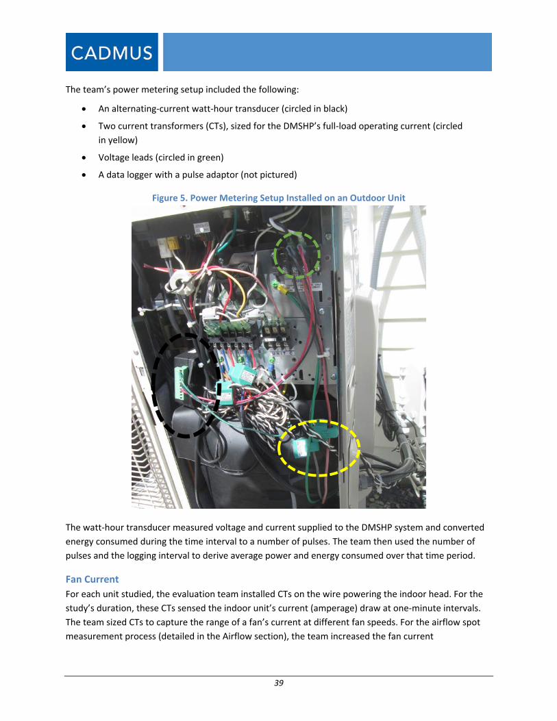
39

The team’s power metering setup included the following:

An alternating‐current watt‐hour transducer (circled in black)

Two current transformers (CTs), sized for the DMSHP’s full‐load operating current (circled

in yellow)

Voltage leads (circled in green)

A data logger with a pulse adaptor (not pictured)

Figure 5. Power Metering Setup Installed on an Outdoor Unit

The watt‐hour transducer measured voltage and current supplied to the DMSHP system and converted

energy consumed during the time interval to a number of pulses. The team then used the number of

pulses and the logging interval to derive average power and energy consumed over that time period.

Fan Current

For each unit studied, the evaluation team installed CTs on the wire powering the indoor head. For the

study’s duration, these CTs sensed the indoor unit’s current (amperage) draw at one‐minute intervals.

The team sized CTs to capture the range of a fan’s current at different fan speeds. For the airflow spot

measurement process (detailed in the Airflow section), the team increased the fan current

40

measurement frequency to read every two seconds, thus increasing the resolution and expediting the

procedure. After the spot test, the team returned the sampling frequency to one‐minute intervals.

Figure 6 shows an installation for a DMSHP system using three indoor heads.

Figure 6. Current Transformers Installed on Fan Wires

Airflow

The evaluation team directly measured the airflow for each indoor unit while on site, using a calibrated

flow hood (i.e., balometer) to capture spot measurements of delivered airflow at each corresponding

fan setting. The team also used specialized frame kits for each balometer, with the instrument’s

geometry modified to better fit a typical DMSHP head. Figure 7 shows a typical flow hood with the

specialized frame kit attached.

41

Figure 7. Balometer

The study population’s various indoor unit models displayed great variability regarding louver settings

and fan‐speed options. To produce repeatable and standardized results, the team conducted airflow

measurements with louvers fixed in place (i.e., not oscillating) and, wherever possible, in fan‐only mode.

The fan‐only setting meant the mode’s discharge conditions generally approximated standard conditions

(i.e., 68 °F and 1 atmosphere). The issue with using other modes to measure airflow is that various units

have algorithms that continuously change fan speeds as unit’s approach temperature settings

interfering with airflow measurement.

The team took airflow measurements at each speed setting on the indoor head’s controller, while

simultaneously collecting one minute of fan current readings at two‐second logging intervals. This

procedure collected a suitable number of current readings for each airflow reading to allow for

correlating airflow and amperage. Logging began once the fan reached a steady state after ramping up

or ramping down the fan motor.

Temperature and Relative Humidity

To calculate heating and cooling loads, the evaluation team measured temperature and relative

humidity across different system points. Using a range of temperature and relative humidity sensors,

the team measured outdoor air, leaving or supply air from the indoor unit, and entering or return air at

the indoor unit. To better understand customers’ operating behaviors, measurements included the

indoor ambient temperature and the relative humidity.

At the outdoor unit, the team installed a temperature and relative humidity sensor, logging values at

one‐minute intervals. Installing this sensor on the unit’s entering air side best measured the

environment in which the unit absorbed or rejected heat. The team also installed a solar shield on the

42

sensor to prevent erroneous readings from solar heating. Figure 8 shows the installation, including the

solar shield.

Figure 8. Outdoor Entering Air Temperature and Relative Humidity Sensor

At the indoor unit’s center, the team installed a temperature and relative humidity sensor to measure

leaving air. The team also installed two additional temperature sensors far left and far right at the supply

grill to gather data used to calculate the average temperature across the supply coil. Figure 9 shows

installation of these sensors.

43

Figure 9. Leaving Air Sensors on a DMSHP Head

The team also installed a temperature and humidity sensor on top of each indoor unit to measure

entering air temperatures and relative humidity. Figure 10 shows the logger and its embedded sensor

zip‐tied on the return grill above the indoor unit.

Figure 10. Entering Air Sensors on a DMSHP Head

Heating Systems

To measure other heating systems’ operating times, the evaluation team used motor loggers, which

either employ an internal AC magnetic field sensor or an external current switch. With both

configurations, the team calibrated the sensors in their installed position, with the heating system

metering point running and operability verified during the initial installation.

Figure 11 shows a motor logger placed on a boiler circulator pump (which also served the space served

by the DMSHP). The image illustrates a similar logger on an oil burner. This same installation can be used

44

to meter a gas valve. The team collected nameplate data from all relevant heating system equipment,

and used these data for various baseline and coincident‐heat calculations.

Figure 11. Boiler System Monitoring

Figure 12 shows the meter deployment for a gas‐fired furnace. To monitor gas consumption, field

technicians installed motor loggers with CTs on both stages of the gas valve. Technicians installed a

similar logger on the blower motor’s power wire. This logger provided backup data on the unit’s run‐

time.

45

Figure 12. Furnace System Monitoring

Site Attributes

To analyze DMSHP performance and to determine their interactions with other cooling or heating

sources, field technicians collected numerous site attributes to calculate approximate heat gain and loss

using the Manual J Residential Load Calculator.

The evaluation team sketched a floor plan for each house and measured each room’s wall lengths and

average ceiling heights to determine room volumes. The team noted general exterior wall construction

as well as space separating the conditioned area (e.g., exterior, conditioned space, ground), including

space above and below each ceiling and floor (e.g., attic, exterior, conditioned space, slab, basement).

Floor plan drawings indicated wall orientations as well as door and window locations. Measurements

included dimensions of all windows and doors, along with notes about their construction, orientation,

and amount of shading.

46

At each site, the team recorded a DMSHP’s make, model, and configuration as well as coincident heating

or cooling sources (e.g., central heating or cooling, space heating, fireplaces). The team also collected

other information, including system type, fuel source, heating or cooling capacity, unit make and model,

control system, and space served. Floor plans showed locations of DMSHP units, space heating or

cooling equipment, and zones served by central systems. This mapping helped in determining overlap

between systems.

Analysis With data collected and a basis established for deriving further quantities from these data, the

evaluation team developed additional methodologies and assumptions to conduct the analysis.

Discussions of these follow.

Airflow

The Airflow section (above) described the relationship between current and airflow. The evaluation

team mapped current to airflow by fitting a curve to spot measurements recorded on site, thus

determining the coefficient and exponent. The team installed metering equipment at 132 sites during

fall 2014, with the remaining 20 Rhode Island sites installed in January 2015. In fall 2015, the team

removed roughly 65 metering installations, and removed and the remaining 85 in spring 2016. For sites

removed in spring 2016, the team used two sets of spot measurements—recorded during fall 2015 and

spring 2016—for these calculations. Sites removed in fall 2015 used a single set of airflow mapping data,

recorded during meter removal.

This approach captured system behaviors at given times and under certain conditions, but the team also

considered variables influencing airflow in addition to fan speeds, such as the amount of material

present on an indoor unit’s air filter, condensed water that can collect on heat exchangers during

cooling, and the position of vanes used to direct conditioned air. Via testing, the team found these

restrictions induced current drops proportional to the drops in volumetric airflow; metering current

suitably accounted for these restrictions. Appendix A fully discusses testing methods, equipment,

and results.

Weather Normalization

The evaluation team weather‐normalized the study results to account for variability between weather

conditions present during the study and during a typical year. The team metered air temperatures and

relative humidity levels adjacent to each DMSHP outdoor unit on site. As sun, wind, snow, and other

variables affected these measurements, the team also collected historical National Oceanic and

Atmospheric Administration data, recorded during the study period by the nearest U.S. Weather Bureau

Army Navy weather station. The team then aligned these data with each site’s meter data, and

calculated average values in 1‐degree temperature bins.

This technique served to illustrate how, on average, participants operated their DMSHPs in various

weather conditions. To normalize data to a typical year, the team gathered National Renewable Energy

Laboratory (NREL) typical meteorological year (TMY3) data from the nearest U.S. Air Force weather

47

station, binned these data by temperature, and multiplied the averages of the study’s value of interest

by the time spent in each bin during a typical year. Where the study found the highest or lowest

temperature observed less extreme than a typical year, the team used data from the nearest observed

temperature bin.

Climate During the Study

As shown in Table 5, summer 2015 experienced a larger number of cooling degree‐days (CDD) than

2014. With the exception of the Norwood, Massachusetts, location, all CDD values from 2015 exceeded

the 10‐year average: winter 2015 was colder than the 10‐year average for all stations, and winter 2016

was milder than the 10‐year average for all stations.

Table 5. Observed Weather During the Study

Station

10 year

CDD(1)

Average

2014

CDD

2015

CDD

10 year

HDD

Average

2014/15

HDD

2015/16

HDD

Norwood Memorial Airport (54704) 641 474 625 5,563 6,685 5,379

Worcester Regional Airport (94746) 569 412 637 6,400 7,050 5,824

Gen E L Logan International Airport (14739) 858 769 921 5,369 6,029 4,804

Lawrence Municipal Airport (94723) 765 609 839 6,462 6,661 5,264

Westover Afb/Metropolitan Airport (14703) 650 483 673 6,270 7,084 5,577

Dillant‐Hopkins Airport (94721) 464 358 490 6,959 7,523 6,143

Brnsbl Muni‐Bman/Pol Fd Ap (94720) 592 488 677 5,569 5,984 5,059

Marthas Vineyard Airport (94724) 528 275 554 5,547 6,208 5,052

North Central State Arpt (64710) 579 423 615 5,945 6,622 4,627

Plymouth Municipal Airport (54769) 667 481 696 5,795 6,433 5,227

Beverly Municipal Airport (54733) 606 532 702 6,068 6,663 5,378

New Bedford Rgnl Airport (94726) 643 471 706 5,671 6,227 5,034

Theodore F Green State Airport (14765) 845 699 945 5,346 6,047 4,778

Block Island State Airport (94793) 623 504 725 5,071 5,609 4,531(1) CDDs were base 65 and based on average daily temperature.

Taking a closer look at temperatures during winter 2015 and 2016, Figure 13 shows the cumulative

distribution of hours spent at various temperatures for the two winters. Winter 2015 had a similarly

shaped distribution of hours, but shifted left by about 8 °F. For both winters, very few hours fell below

0°F. The midpoint of distribution (i.e., half of the hours) was about 30°F during winter 2015 and about

38°F during winter 2016.

48

Figure 13. Cumulative Distribution of Winter Hours Versus Temperature Bin

49

Error! Not a valid bookmark self‐reference. shows the distribution of summer hours at various

temperatures, with very few hours at 90°F or greater.

Figure 14. Cumulative Distribution of Summer Hours Versus Temperature Bin

Manual J: Residential Load Calculation

The evaluation team examined how contractors sized DMSHPs and whether the units could meet the

heating and cooling requirements for the spaces they served. To answer this, the team calculated

50

thermal loads using an abridged Manual J31 calculator, in conjunction with the Manual J: Residential

Load Calculation textbook published by the American National Standards Institute/Air Conditioning

Contractors of America (ANSI/ACCA, Version 2, Eighth Edition). These calculations estimated the highest

steady state heating and cooling loads that DMSHPs would experience at design conditions.

An industry‐approved method for establishing the sizing of heating and cooling systems, Manual J

provides a recommended resource for contractors’ use (either directly by using an abridged spreadsheet

or indirectly by using the plethora of available third‐party software). For this study, the team used the

ANSI/ACCA Manual J’s electronic spreadsheet.

Through discussions with homeowners, the team established boundaries on spaces served by DMSHP

units. These boundaries, varying from large rooms to regions of a house to an entire house, proved

crucial for gathering an appropriate amount of data from each house. During these discussions, the

team focused on homeowners’ requests to installing contractors rather than in situ performance to

draw appropriate comparisons.

Practical limitations on data collected on site dictated the analysis detail level. For example, thicknesses

and types of wall insulation often cannot be determined without opening holes in a wall. Given such

limitations, the team assessed the type and quantity of insulation present in basements and attics, and

consulted homeowners for further information. When the former proved difficult, the team used

applicable building codes and typical construction practices.

To establish outdoor design conditions for Manual J, the team used the arithmetic mean of the

geographic latitude and longitude of the entire sample population, and then selected the ACCA Manual J

location closest to this point. This method provided an average condition, but gave a good indication of

the unit’s relative capacity to the space it served. The resulting location (i.e., Framingham,

Massachusetts) had a summer 1% dry bulb temperature of 88°F and a winter 99% dry bulb temperature

of 6 °F. The team used these values to calculate heat gain and heat loss in spaces served by DMSHPs.

Savings

To answer a key research question (“How much energy is being saved with the average installation of a

DMSHP through the programs?”), the evaluation team developed a methodology to estimate savings for

numerous heating and cooling baseline equipment options. Alternative equipment options for heating

included the following:

31 Air Conditioning Contractors of America. ACCA Speed‐Sheet for Manual J (Abridged Edition).PowerPoint

presentation and corresponding Microsoft Excel workbook. June 22, 2015. Available online:

http://www.acca.org/communities/community‐

home/librarydocuments/viewdocument?DocumentKey=0bc73e80‐6c3c‐43cb‐bdb2‐43316a380fa4

http://www.acca.org/HigherLogic/System/DownloadDocumentFile.ashx?DocumentFileKey=b77bcc44‐be9c‐

45d5‐b23f‐6774e5663ed2&forceDialog=1

51

Furnace (assuming 85% and 90% AFUE, MA 2013–2015 TRM)

Boiler (assuming 82% AFUE, MA 2013–2015 TRM)

HSPF 7.7 DMSHP (federal minimum efficiency standard for central ASHPs prior to

January 1, 2015)

HSPF 8.2 DMSHP (current federal minimum efficiency standard for central ASHPs, effective

January 1, 2016)

Electric resistance baseboard heat or furnace (COP=1.0)

For cooling, alternative equipment options included the following:

EER 9.8 Window AC (current federal standard)

SEER 13.0 Central AC with duct losses of 15% (current federal minimum efficiency standard for

central ACs and duct‐loss estimate based on the MA 2013–2015 TRM)

SEER 13.0 DMSHP (federal minimum efficiency standard for central ACs and for central ASHPs

prior to January 1, 2015)

SEER 14.5 DMSHP (from a team estimate from market research for lowest‐cost DMSHP options

available, reflecting an increase from the current federal minimum efficiency standard of

SEER 14.0, effective January 1, 2016)

To develop the savings methodology, the team assumed that the DMSHP heating and cooling capacity

remained constant in each baseline scenario. The numerator of SEER or HSPF value (per the Seasonal

Efficiency Metrics section) represented the capacity—a metered and quantifiable parameter. To

estimate savings for the most common baseline scenario (i.e., a lower‐efficiency DMSHP), the team used

metered energy consumption. The following equations show the savings calculation approach.

Cooling savings equation for electric baseline system:

∆

Heating savings equation for electric baseline system:

∆

Where:

52

∆kWh_COOL = Reduction in annual kWh cooling consumption of heat pump equipment

∆kWh_HEAT = Reduction in annual kWh heating consumption of heat pump equipment

T_H = Highest observed outdoor dry bulb temperature with cooling during cooling season;

heating during heating season from a local weather station

T_L = Lowest observed outdoor dry bulb temperature with cooling during cooling season;

heating during heating season from a local weather station

kWh_METERED = Logged energy consumption

EER_BASE = Instantaneous efficiency of baseline equipment (varies with outdoor conditions)

EER_EE = Instantaneous efficiency of installed equipment (varies with outdoor conditions)

Hours_TMY = Total count of TMY hours in each temperature bin from a local weather station

Hours_ACTUAL = Total count of observed hours in each temperature bin from a local weather station

This study directly measured instantaneous efficiency to evaluate DMSHP performance. The team

initially used metered efficiency and then decremented the baseline unit’s efficiency by a proportional

amount. This proved mathematically equivalent to the method described below.

The team reviewed manufacturers’ specification data to determine baseline DMSHP performance

(e.g., 13.0 or 14.5 SEER) versus temperature, and developed heating and cooling performance curves

(eer versus temperature). In many cases, manufacturer‐rated SEER and HSPF values differed from

DMSHPs’ actual seasonal operations (see Figure 50 and Figure 51). The team assumed, however, that

the energy‐consumption difference between a baseline DMSHP and efficiency DMSHP correlated to the

ratio of AHRI‐rated SEER and HSPF values.

In other words, if a 20.0 SEER DMSHP had an actual operating efficiency of 15.0 SEER, the team did not

calculate savings relative to a 13.0‐ or 14.5‐SEER baseline DMSHP. Rather, the team assumed the

baseline DMSHP would have operated less efficiently, maintaining the following relationship as a

function of temperature (T):

To estimate savings from energy consumption, the evaluation team only used energy consumed when

the DMSHP actually provided heating or cooling. This effectively removed energy consumed due to

various operation types that would not generate savings (e.g., fan‐only operation).

The team assumed a baseline efficiency DMSHP would have consumed energy in the same way when

operating in a mode that would not provide heating or cooling. The possibility certainly exists that a

baseline DMSHP could use more energy (e.g., through less efficient defrost control sequencing or less‐

efficient dehumidification), but the team did not have operational data of baseline DMSHPs to estimate

savings. Thus, the final DMSHP savings estimates could be conservative.

53

The team identified heating and cooling mode operations through site‐by‐site review of raw meter data.

Primarily, the review determined the indoor unit airflow (i.e., in some modes, indoor fans did not run)

and the enthalpy differential from supply and return air sensors to identify operation for every metered

interval.

To estimate savings for other system types, the team followed a similar approach, assuming that

alternative equipment would have provided capacity equivalent to that provided by the DMSHP. Table 6

summarizes the savings methodologies used for the most common baseline options and describes

additional adjustments to the final savings estimate for each scenario (e.g., a DMSHP that offsets heat

delivered by a fossil fuel system provides positive fuel savings but negative kWh savings). Additional

zonal savings could be available from only heating occupied spaces, particularly during shoulder months

with low heating loads and homeowners possibly heating only with the DMSHP. This study did not

directly capture such savings.

Table 6. Savings Calculation Methodology for Alternative Heating/Cooling Equipment

Baseline Savings Methodology Savings Adjustments

Electric

Resistance

Heating savings based on total heating capacity

provided by DMSHPs in winter and a difference in

efficiency (1.0 COP = 3.412 HSPF)

Subtract energy use from savings estimate if

use did not provide heat (e.g., defrost,

standby power)

Furnace


provided by DMSHPs in winter, converted to

MMBTUs and adjusted by furnace efficiency

Subtract total electrical energy use of

DMSHP from estimated fan energy use of

associated furnace runtime reductions from

central furnace fan

Boiler


provided by DMSHP in winter, converted to

MMBTUs and adjusted by boiler efficiency

Subtract total electrical energy use of

DMSHP; assume no benefit (reduction) in

boiler circulation‐pump energy use.

Window AC Same methodology used for DMSHPs (ratio of

window AC AHRI EER rating to DMSHP SEER rating) None

Central AC

Same methodology used for DMSHP (ratio of

window AC AHRI EER rating to DMSHP SEER rating)

with additional 15% duct losses

None

To estimate summer peak demand savings, the team determined total weather‐normalized energy

consumption (kWh) and savings from all meter data during the demand period and kWh by the total

number of hours during the demand period. The four‐hour summer demand period begins at 1:00 PM,

June through August, on non‐holiday weekdays. The two‐hour winter demand period begins at 5:00 PM,

December through January, on non‐holiday weekdays. To calculate savings, the team followed the

energy‐savings methodology.

54

Results

This section presents the evaluation’s general findings and summarizes data in the context of each

research objective. The graphs and tables show results across the population of DMSHPs studied. The

data underlying the graphs was derived from detailed analysis of time series of data for each system

including power consumed and cooling and heating provided. Appendix D shows an example of a time

series of a DMSHP.

Load Shapes Figure 15, Figure 16, and Figure 17 show metered units’ average power usage of for winter 2015,32

summer 2015,33 and winter 2016, respectively, by time of day. Average heating demand ranges from

150 to 300 watts, with a slight shape to the curve, a peak at 8:00 AM, and a small relative peak at

8:00 PM. The cooling curve shows much more shape and variation, with a relative minimum at 4:00 AM

and a relative maximum at 4:00 PM. The cooling load shape displays a peak of approximately 160 watts.

Figure 15. Winter 2015 Average Power Consumption vs. Time of Day, N=99

32 October 15 to April 15.

33 May 15 to September 30.

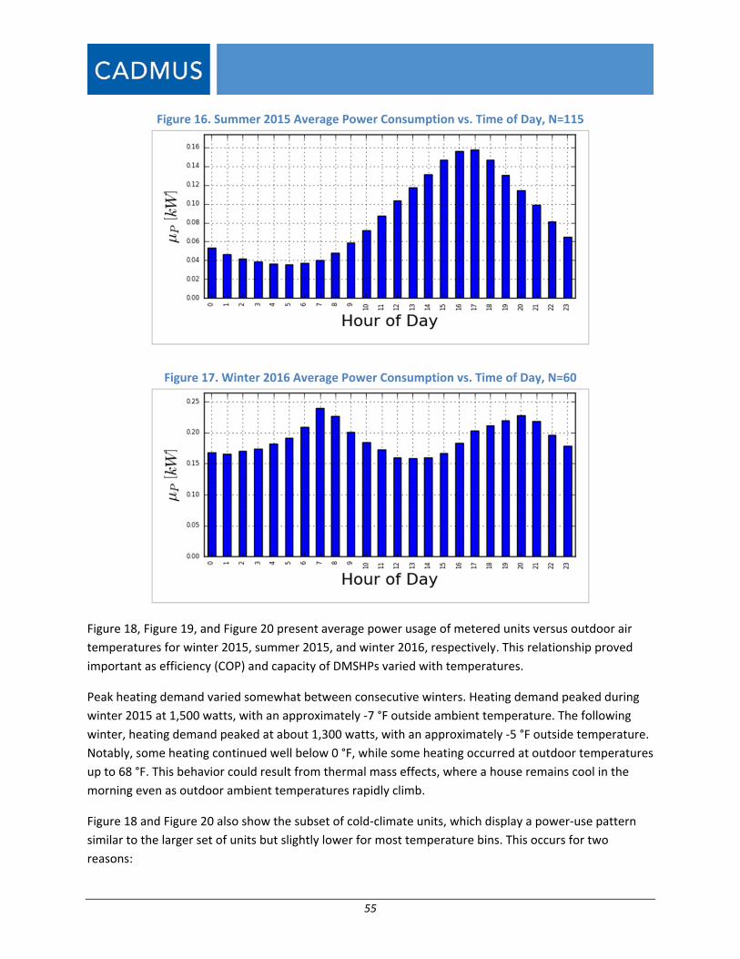
55

Figure 16. Summer 2015 Average Power Consumption vs. Time of Day, N=115

Figure 17. Winter 2016 Average Power Consumption vs. Time of Day, N=60

Figure 18, Figure 19, and Figure 20 present average power usage of metered units versus outdoor air

temperatures for winter 2015, summer 2015, and winter 2016, respectively. This relationship proved

important as efficiency (COP) and capacity of DMSHPs varied with temperatures.

Peak heating demand varied somewhat between consecutive winters. Heating demand peaked during

winter 2015 at 1,500 watts, with an approximately ‐7 °F outside ambient temperature. The following

winter, heating demand peaked at about 1,300 watts, with an approximately ‐5 °F outside temperature.

Notably, some heating continued well below 0 °F, while some heating occurred at outdoor temperatures

up to 68 °F. This behavior could result from thermal mass effects, where a house remains cool in the

morning even as outdoor ambient temperatures rapidly climb.

Figure 18 and Figure 20 also show the subset of cold‐climate units, which display a power‐use pattern

similar to the larger set of units but slightly lower for most temperature bins. This occurs for two

reasons:

56

1. Cold climate units, with only single heads, have lower capacity, and are rated at higher

efficiencies (see Table 4).

2. Cooling demand (Figure 19) increased with outside air temperatures until peaking at about

760 watts at 93 °F.

Particularly, cooling occurred down to outdoor temperatures in the 60s, which could result from

thermal mass effects, where a house stays warm in the evening when outdoor temperatures rapidly

drop, or from internal loads (e.g., solar).

Figure 18. Winter 2015 Average Power Consumption While Heating vs. Outdoor Air Temperature

57

Figure 19. Summer 2015 Average Power Consumption While Cooling vs. Outdoor Air Temperature, N=114

Figure 20. Winter 2016 Average Power Consumption While Heating vs. Outdoor Air Temperature, N=57

Figure 21, Figure 22, Figure 23, Figure 24, and Figure 25 show a seasonal time series of average power

demand for winter 2015, summer 2015, and winter 2016 for all units and, separately, for cold climate

58

units. Seasonal DMSHP heating use widely varies, but not nearly as much as summer usage. During

summer periods with milder outdoor temperatures, DMSHP units largely remain off. The time series

graphs for all units and for cold climate units produced similar results.

Figure 21. Winter 2015 Average Power Consumption vs. Time, N=99

Figure 22. Winter 2015 Average Power Consumption vs. Time, N=51, Cold Climate Units

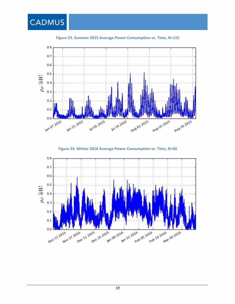
59

Figure 23. Summer 2015 Average Power Consumption vs. Time, N=115

Figure 24. Winter 2016 Average Power Consumption vs. Time, N=60

60

Figure 25. Winter 2016 Average Power Consumption vs. Time, N=35, Cold Climate Units

Table 7 shows units’ low coincidence factors (CF) for both summer and winter peak periods, at

precisions less than 1%. Essentially, many units remained off, and those running did not operate at full

capacity, resulting in low CFs.

Table 7. CFs for Peak Winter and Summer Periods

Season Mean CF Precision [%]

Winter 2015 0.130 0.71

Summer 2015 0.181 0.99

Winter 2016 0.120 0.94

Operating Hours Table 8 shows simple run‐time hours for metered DMSHPs, with a unit logged as running if its power

draw exceeded a threshold standby power of 60W. Looking at the nominal heating season, the average

unit ran about 27% of the time (793 hours) during 2015, and about 24% of the time (703 hours) during

2016. Note that an operating hour differs from a full‐load hour in that an operating hour simply means

that the unit remained on at some capacity, whereas a full‐load hour indicates the unit ran at full

capacity.

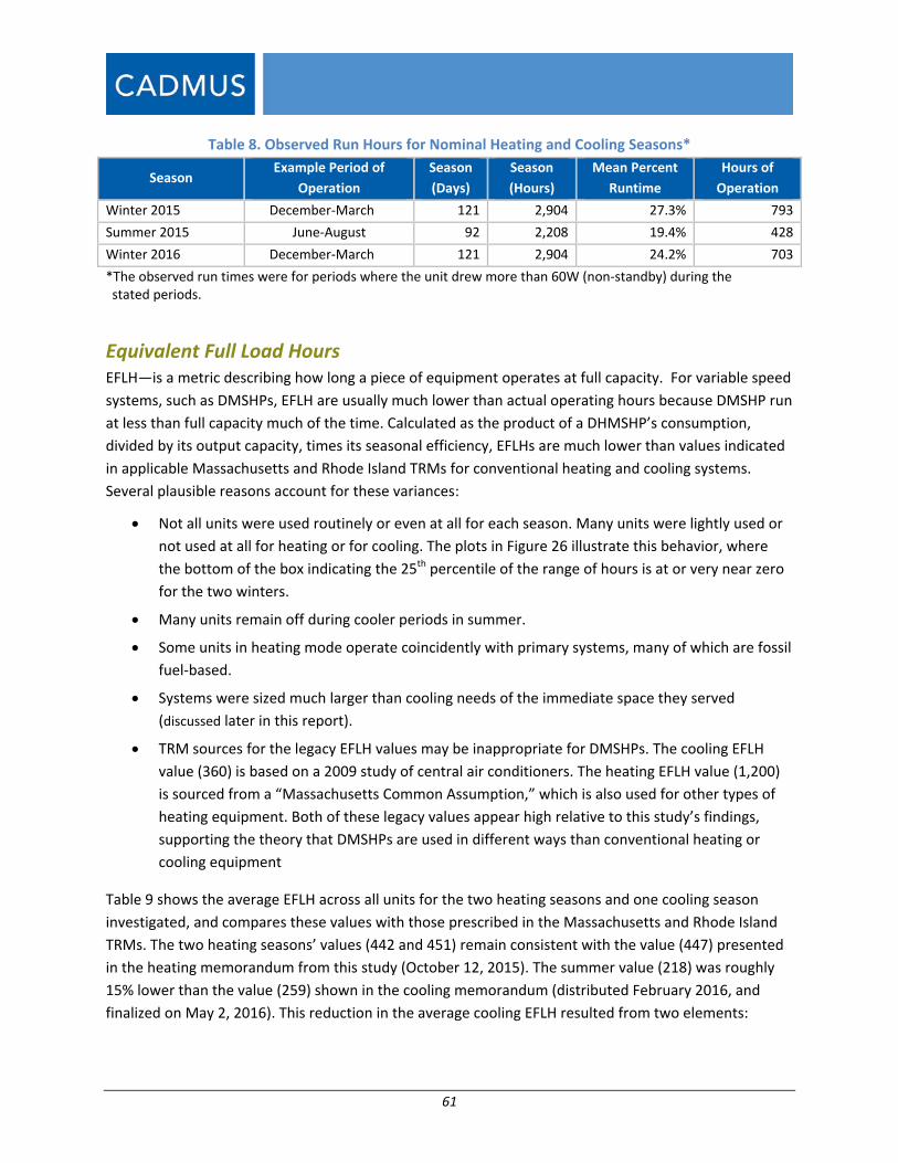
61

Table 8. Observed Run Hours for Nominal Heating and Cooling Seasons*

Season Example Period of

Operation

Season

(Days)

Season

(Hours)

Mean Percent

Runtime

Hours of

Operation


Summer 2015 June‐August 92 2,208 19.4% 428


*The observed run times were for periods where the unit drew more than 60W (non‐standby) during the stated periods.

Equivalent Full Load Hours EFLH—is a metric describing how long a piece of equipment operates at full capacity. For variable speed

systems, such as DMSHPs, EFLH are usually much lower than actual operating hours because DMSHP run

at less than full capacity much of the time. Calculated as the product of a DHMSHP’s consumption,

divided by its output capacity, times its seasonal efficiency, EFLHs are much lower than values indicated

in applicable Massachusetts and Rhode Island TRMs for conventional heating and cooling systems.

Several plausible reasons account for these variances:

Not all units were used routinely or even at all for each season. Many units were lightly used or

not used at all for heating or for cooling. The plots in Figure 26 illustrate this behavior, where

the bottom of the box indicating the 25th percentile of the range of hours is at or very near zero

for the two winters.

Many units remain off during cooler periods in summer.

Some units in heating mode operate coincidently with primary systems, many of which are fossil

fuel‐based.

Systems were sized much larger than cooling needs of the immediate space they served

(discussed later in this report).

TRM sources for the legacy EFLH values may be inappropriate for DMSHPs. The cooling EFLH

value (360) is based on a 2009 study of central air conditioners. The heating EFLH value (1,200)

is sourced from a “Massachusetts Common Assumption,” which is also used for other types of

heating equipment. Both of these legacy values appear high relative to this study’s findings,

supporting the theory that DMSHPs are used in different ways than conventional heating or

cooling equipment

Table 9 shows the average EFLH across all units for the two heating seasons and one cooling season

investigated, and compares these values with those prescribed in the Massachusetts and Rhode Island

TRMs. The two heating seasons’ values (442 and 451) remain consistent with the value (447) presented

in the heating memorandum from this study (October 12, 2015). The summer value (218) was roughly

15% lower than the value (259) shown in the cooling memorandum (distributed February 2016, and

finalized on May 2, 2016). This reduction in the average cooling EFLH resulted from two elements:

62

Use of local TMY data for this report, in contrast with statewide TMY data used in the memo

The evaluation team removed standby power usage and off‐season conditioning from this

report’s analysis

The right column of shows the EFLH for the top 25% of units for each seasons. These heating season

values average close the TRM value and the cooling value exceeds the TRM value.

Table 9. Average EFLH

Season 2013‐2015 MA TRM 2014 RI TRM Average Study EFLH Average of Top 25% of

Measured EFLH

Winter 2015 1,200 1,200 442 1,275

Summer 2015 360 360 218 499

Winter 2016 1,200 1,200 451 1,117

Figure 26 presents DMSHP usage by season, shows a wide variation in units’ EFLH, particularly for

heating. Figure 27 shows a similar pattern for cold climate units.

Figure 26. DMSHP EFLH vs. Season

63

Figure 27. DMSHP EFLH vs. Season, Cold Climate Units

Figure 28 examines this variation more closely and shows that units purchased for “both heating and

cooling” were used much more for heating than units purchased as “cooling only.” Winter 2016 was

milder than winter 2015, and winter 2015 had very deep snow falls that buried units for part of the

winter. Units operated more efficiently during 2016 (see Figure 52). This resulted in lower EFLH for

users intending “both heating and cooling” in Winter 2016. During winter 2016, units purchased for

“cooling only” saw some heating usage.

64

Figure 28. DMSHP EFLH vs. Purchase Intent and Season

Figure 29. DMSHP EFLH vs. Purchase Intent and Season, Cold Climate Units

For electric savings, actual DMSHP performance was used, with the baseline unit’s efficiency

decremented from its nameplate rating by the same proportion that the efficient unit’s performance

differed from its rating. Cooling savings increased with lower‐efficiency baselines. Calculation for savings

65

relative to a central air conditioner baseline included a 15% duct loss, which decreases net efficiency. As

discussed, these savings values were based on the baseline and on the DMSHP providing the same

amount of heating (and cooling); they did not include zonal savings gained in some homes.

Table 10. Energy Savings, Each Baseline Applied to All Sites


Size

Electric Usage

of DMSHP

[kWh]

Baseline

Energy

Reduction

Net Energy

Savings

Precision at

90% Confidence

[%]

Winter

2015

90% AFUE Furnace(1)

98

683 4.87 MMBtu 2.54 MMBtu 37





Electric Resistance 683 1,092 kWh 409 kWh 48

Summer

2015

EER 9.8 Window AC

114

159 213 kWh 54 kWh 15




Winter

2016

90% AFUE Furnace

60

763 6.9 MMBtu 4.3 MMBtu 37





Electric Resistance 763 1,547 kWh 784 kWh 42(1) Duct losses were assumed as 15%. (2) Baseline efficiency prescribed by relevant Massachusetts (2013–2015) and Rhode Island (2015) TRMs applicable when beginning this study.

Table 11 shows average winter34 and summer35 peak demand savings. The evaluation team calculated

peak savings as follows:

Calculating energy savings during respective summer and winter peak periods.

Dividing savings by peak hours to yield average peak demand savings.

As with consumption savings, electrical resistance heating provided the highest savings; these declined

with the baseline unit’s increasing efficiency.

34 The MA (2016–2018) and RI (2016) TRMs defined winter peak as 5:00 PM to 7:00 PM on non‐holiday

weekdays in December and January.

35 The MA (2016–2018) and RI (2016) TRMs defined summer peak as 1:00 PM to 5:00 PM on non‐holiday

weekdays in June, July, and August.

66

Table 11. Peak Demand Savings, Each Baseline Applied to All Sites


Size

Electric Usage

of DMSHP

[kW]

Baseline Power

Reduction [kW]

Average Peak

Period Demand

Savings [kW]

Precision at

90% Confidence

[%]

Winter

2015

90% AFUE Furnace

98

0.21 0 ‐0.21 33

85% AFUE Furnace 0.21 0 ‐0.21 33

82% AFUE Boiler 0.21 0 ‐0.21 33

HSPF 7.7 DMSHP 0.21 0.28 0.07 22

HSPF 8.2 DMSHP 0.21 0.26 0.05 22


Summer

2015

EER 9.8 Window AC

114

0.11 0.15 0.04 16

SEER 13.0 Central AC 0.11 0.20 0.09 15

SEER 13.0 DMSHP 0.11 0.05 0.06 15

SEER 14.5 DMSHP 0.11 0.07 0.04 15

Winter

2016

90% AFUE Furnace

60

0.25 0 ‐0.25 34

85% AFUE Furnace 0.25 0 ‐0.25 34

82% AFUE Boiler 0.25 0 ‐0.25 34

HSPF 7.7 DMSHP 0.25 0.33 0.08 24

HSPF 8.2 DMSHP 0.25 0.31 0.06 25


We did not assume electricity credit for reducing the operation of a baseline furnace fan or boiler pump.

This results in a conservative assumption as some reduction in fan and pump use likely occurred.

Without conducting a pre‐post DMSHP study, identifying the timing and amount of that reduction

proves difficult. On average, a standard boiler pump uses about 120 kWh per year,36 and a fan uses

about 440 kWh37 per year for heating. Where a DMSHP can be used as the primary heating source, this

electricity use could be substantially reduced, increasing consumption and demand savings, and

decreasing DMSHP net electricity use.

As in Table 10, Table 12 shows savings for each baseline, but it applies the baseline only to homes that

indicated that specific baseline, based on survey responses. Sample sizes were much smaller than those

used in Table 10, and relative precisions were much larger (worse). Calculating the savings this way drew

upon several stakeholder’s hypotheses that users would behave differently due to different survey

responses. The evaluation team suggests variability in usage is already very high, and that dividing the

population into small subpopulations based on these survey responses does not yield meaningful

information. Savings were generally lower, though much higher for electrical resistance heat.

36 Boiler pump study

37 AHRI average = 365W/ 1,000 CFM. At 1,200 CFM and 1,000 run time hours, this is 438 kWh.

67

Table 12. Energy Savings, Baseline Applied Based on Survey Responses and Existing Systems


Size

Electric Usage

of DMSHP

[kWh]

Baseline

Energy

Reduction

Average Energy

Savings

Precision at

90% Confidence

[%]

Winter

2015

90% AFUE Furnace 10 702 3.79 MMBtu 1.39 MMBtu 120


82% AFUE Boiler 27 786 5.51 MMBtu 2.83 MMBtu 68

HSPF 7.7 DMSHP 37 425 588 kWh 163 kWh 41


Electric Resistance 3 732 1,130 kWh 398 kWh 334

Summer

2015

EER 9.8 Window AC 9 306 399 kWh 93 kWh 33

SEER 13.0 Central

AC 7 103 198 kWh 95 kWh 50

SEER 13.0 DMSHP 38 189 292 kWh 103 kWh 26

SEER 14.5 DMSHP 38 189 262 kWh 73 kWh 27

Winter

2016



82% AFUE Boiler 14 1,056 9.78 MMBtu 6.17 MMBtu 82



Electric Resistance 2 1,202 2,980 kWh 1,778 kWh 35

Table 13 shows the average winter38 and summer39 peak demand savings for the same survey‐based

baseline. The demand savings generally were lower than in Table 11, but relative precision values were

much higher (worse).

Table 13. Peak Demand Savings, Baseline Applied Based on Survey Responses and Existing Systems


Size

Electric

Usage of

DMSHP [kW]

Baseline Power

Reduction [kW]

Average Peak

Period Demand

Savings [kW]

Precision at

90% Confidence

[%]

Winter

2015

90% AFUE Furnace 10 0.28 0 ‐0.28 53

85% AFUE Furnace 10 0.28 0 ‐0.28 53

82% AFUE Boiler 27 0.25 0 ‐0.25 38

HSPF 7.7 DMSHP 37 0.12 0.16 0.04 kW 48

HSPF 8.2 DMSHP 37 0.12 0.15 0.03 kW 48

38 The Massachusetts (2016–2018) and Rhode Island (2016) TRMs defined winter peak as 5:00 PM to 7:00 PM on

non‐holiday weekdays in December and January.

39 The Massachusetts (2016–2018) and Rhode Island (2016) 2016–2018 TRMs defined summer peak as 1:00 PM

to 5:00 PM on non‐holiday weekdays in June, July, and August.

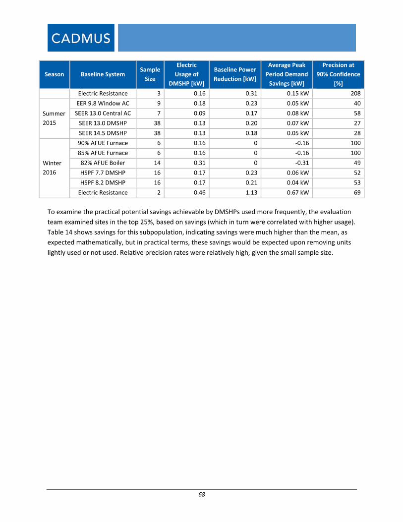
68


Size

Electric

Usage of

DMSHP [kW]

Baseline Power

Reduction [kW]

Average Peak

Period Demand

Savings [kW]

Precision at

90% Confidence

[%]

Electric Resistance 3 0.16 0.31 0.15 kW 208

Summer

2015

EER 9.8 Window AC 9 0.18 0.23 0.05 kW 40

SEER 13.0 Central AC 7 0.09 0.17 0.08 kW 58

SEER 13.0 DMSHP 38 0.13 0.20 0.07 kW 27

SEER 14.5 DMSHP 38 0.13 0.18 0.05 kW 28

Winter

2016

90% AFUE Furnace 6 0.16 0 ‐0.16 100

85% AFUE Furnace 6 0.16 0 ‐0.16 100

82% AFUE Boiler 14 0.31 0 ‐0.31 49

HSPF 7.7 DMSHP 16 0.17 0.23 0.06 kW 52

HSPF 8.2 DMSHP 16 0.17 0.21 0.04 kW 53

Electric Resistance 2 0.46 1.13 0.67 kW 69

To examine the practical potential savings achievable by DMSHPs used more frequently, the evaluation

team examined sites in the top 25%, based on savings (which in turn were correlated with higher usage).

Table 14 shows savings for this subpopulation, indicating savings were much higher than the mean, as

expected mathematically, but in practical terms, these savings would be expected upon removing units

lightly used or not used. Relative precision rates were relatively high, given the small sample size.

69

Table 14. Energy Savings, Each Baseline Applied to All Sites, Top 25%


Size

Electric Usage

of DMSHP

[kWh]

Baseline

Energy

Reduction

Average

Energy

Savings

Precision at

90%

Confidence [%]

Winter

2015

90% AFUE Furnace

25

1,414 14.7 MMBtu 9.84 MMBtu 22

85% AFUE Furnace 1,414 15.5 MMBtu 10.70 MMBtu 22

82% AFUE Boiler 1,414 13.1 MMBtu 8.86 MMBtu 22

HSPF 7.7 DMSHP 1,894 2,536 kWh 642 kWh 10


Electric Resistance 1,414 3,287 kWh 1,873 kWh 24

Summer

2015

EER 9.8 Window AC

29

358 484 kWh 126 kWh 12




Winter

2016

90% AFUE Furnace

15

1,566 18.68 MMBtu 13.34 MMBtu 30

85% AFUE Furnace 1,566 19.78 MMBtu 14.44 MMBtu 30

82% AFUE Boiler 1,566 17.43 MMBtu 12.09 MMBtu 31



Electric Resistance 1,566 4,188 2,622 kWh 33

Similarly, Table 15 shows demand savings for the top 25% of sites.

Table 15. Peak Demand Savings, Each Baseline Applied to All Sites, Top 25%


Size

Electric

Usage of

DMSHP

[kW]

Baseline

Power

Reduction

[kW]

Average Peak

Period

Demand

Savings [kW]

Precision at

90%

Confidence

[%]

Winter

2015

HSPF 7.7 DMSHP

25

0.62 0.82 0.20 kW 13

HSPF 8.2 DMSHP 0.56 0.70 0.14 kW 14

Electric Resistance 0.47 1.02 0.55 kW 19

Summer

2015

EER 9.8 Window AC

29

0.24 0.33 0.09 kW 13

SEER 13.0 Central AC 0.25 0.45 0.20 kW 11

SEER 13.0 DMSHP 0.23 0.36 0.13 kW 12

SEER 14.5 DMSHP 0.22 0.31 0.09 kW 13

Winter

2016

HSPF 7.7 DMSHP

15

0.61 0.80 0.19 kW 12

HSPF 8.2 DMSHP 0.61 0.76 0.15 kW 15

Electric Resistance 0.54 1.64 1.1 kW 26

Using baselines weighted from the previously published baseline memorandum, the evaluation team

calculated average weighted savings for each of the three studied seasons, calculated for a single and a

weighted baseline (as shown in Table 16). In general, winter 2016, with data unaffected by 2015’s large

70

snowfalls, realized higher savings. The specific baselines show savings similar to or somewhat higher

than the single baselines. Table 17 shows the non‐fuel switching savings, which were far lower than fuel

switching because baseline DMSHP savings are lower than those from fuel heating.

71

Table 16. Weighted Average Savings, Fuel Switching

Fuel Switching Single baseline Specific baseline

Season

Baseline System

Base Eff.

Efficiency Metric

Savings Units

n Mean Savings

Mean Savings [kWh]

Population with

Baseline [%]

Expected Baseline Savings [kWh]

Precision [%]

Sample Size

Mean Savings

Mean Savings [kWh]

Pop. with

Baseline [%]


Precision [%]

Winter 2015 Furnace 0.85 AFUE MMBtu

98

2.83 829 13% 108 36 10 1.62 475 13% 62 109


ER 1 COP kWh 409 409 4% 16 48 3 398 398 4% 15 334

DHP 7.7 HSPF kWh 224 224 48% 108 21 37 163 163 48% 78 41

Weighted Total

100% 458 31 100% 446 71

Summer 2015

Window AC

9.8 EER kWh

114

54 54 17% 9 15 9 93 93 17% 16 33

CAC 13 SEER kWh 129 129 13% 17 14 7 95 95 13% 12 50

DHP 13 SEER kWh 86 86 70% 61 14 38 103 103 70% 72 26

Weighted Total

100% 86 14 100% 100 30

Winter 2016 Furnace 0.85 AFUE MMBtu

60

4.70 1378 16% 218 36 6 3.05 894 16% 141 103


ER 1 COP kWh 784 784 5% 41 42 2 1778 1778 5% 94 35

DHP 7.7 HSPF kWh 226 226 42% 95 22 16 176 176 42% 74 55

Weighted Total

100% 768 31 100% 975 71

72

Table 17. Weighted Average Savings, Non‐Fuel Switching

Non Fuel Switching Single Baseline Specific Baseline

Season

Baseline System

Base Eff.

Effi‐ciency Metric

Savings Units

n Mean Sav‐ings

Mean Saving

s [kWh]

Pop. with

Baseline [%]


Precision [%]

Sample Size

Mean Savings

Mean Savings [kWh]

Pop. with

Baseline [%]


Precision [%]

Winter

2015

ER 1 COP kWh 98

409 409 8% 31 48 3 398 398 8% 30 334

DHP 7.7 HSPF kWh 224 224 93% 207 21 37 163 163 93% 150 41

Weighted Total

100% 238 23 100% 180 63

Summer 2015 Window

AC 9.8 EER kWh

114

54 54 17% 9 15 9 93 93 17% 16 33

CAC 13 SEER kWh 129 129 13% 17 14 7 95 95 13% 12 50

DHP 13 SEER kWh 86 86 70% 61 14 38 103 103 70% 72 26

Weighted Total

100% 86 14 100% 100 30

Winter

2016

ER 1 COP kWh 60

784 784 11% 87 42 2 1778 1778 11% 198 35

DHP 7.7 HSPF kWh 226 226 89% 201 22 16 176 176 89% 156 55

Weighted Total

100% 288 25 100% 354 53

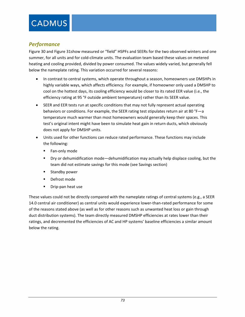
73

Performance Figure 30 and Figure 31show measured or “field” HSPFs and SEERs for the two observed winters and one

summer, for all units and for cold‐climate units. The evaluation team based these values on metered

heating and cooling provided, divided by power consumed. The values widely varied, but generally fell

below the nameplate rating. This variation occurred for several reasons:

In contrast to central systems, which operate throughout a season, homeowners use DMSHPs in

highly variable ways, which affects efficiency. For example, if homeowner only used a DMSHP to

cool on the hottest days, its cooling efficiency would be closer to its rated EER value (i.e., the

efficiency rating at 95 °F outside ambient temperature) rather than its SEER value.

SEER and EER tests run at specific conditions that may not fully represent actual operating

behaviors or conditions. For example, the SEER rating test stipulates return air at 80 °F—a

temperature much warmer than most homeowners would generally keep their spaces. This

test’s original intent might have been to simulate heat gain in return ducts, which obviously

does not apply for DMSHP units.

Units used for other functions can reduce rated performance. These functions may include

the following:

Fan‐only mode

Dry or dehumidification mode—dehumidification may actually help displace cooling, but the

team did not estimate savings for this mode (see Savings section)

Standby power

Defrost mode

Drip‐pan heat use

These values could not be directly compared with the nameplate ratings of central systems (e.g., a SEER

14.0 central air conditioner) as central units would experience lower‐than‐rated performance for some

of the reasons stated above (as well as for other reasons such as unwanted heat loss or gain through

duct distribution systems). The team directly measured DMSHP efficiencies at rates lower than their

ratings, and decremented the efficiencies of AC and HP systems’ baseline efficiencies a similar amount

below the rating.

74

Figure 30. Measured Seasonal Efficiencies

Figure 31. Measured Seasonal Efficiencies, Cold Climate Units

75

Figure 32. Winter 2015 Measured HSPF vs. EFLH, N=86

Figure 33. Summer 2015 Measured SEER vs. EFLH, N=113

Figure 320 and Figure 341 show a substantial increase in HSPF from winter 2015 to winter 2016. This

increase could result from variations in snowfall between the two winters; these can obstruct the

76

outdoor unit’s airflow. The top 25% of the units used lightly (<100 EFLH) and heavily (>500 EFLH) both

approached or exceeded a 10.0 HSPF—the average rating of metered units.

Figure 34. Winter 2016 Measured HSPF vs. EFLH, N=57

Figure 352 through Figure 40 present DMSHP efficiency plots by the number of indoor heads per

outdoor unit and by EFLH. The efficiency range in these plots tightened when moving from one head to

three heads, but this likely resulted from the decreasing sample size with an increasing number of

heads. Efficiency appeared to decrease somewhat with an increasing number of heads, but partly

resulted from the lower ratings of these multi‐head systems. For single‐head units, the 75th percentile of

SEER (20.0) was near the average rated value. For winter 2016, the 75th percentile of HSPF was well

above 10.0 for single‐head units.

77

Figure 35. Winter 2015 HSPF vs. System Configuration, N=87

Figure 36. Summer 2015 SEER vs. System Configuration, N=114

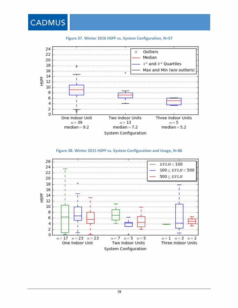
78

Figure 37. Winter 2016 HSPF vs. System Configuration, N=57

Figure 38. Winter 2015 HSPF vs. System Configuration and Usage, N=86

79

Figure 39. Summer 2015 SEER vs. System Configuration and Usage, N=113

Figure 40. Winter 2016 HSPF vs. System Configuration and Usage, N=57

Units purchased for “cooling only” exhibited the highest measured SEER values, with the 75th percentile

well above 20.0. A similar link did not become apparent between purchase intent and measured HSPF

(see Figure 41). The same held true for cold climate units (see Figure 42).

80

Figure 41. Seasonal Efficiencies vs. Purchase Intent

Figure 42. Seasonal Efficiencies vs. Purchase Intent, Cold Climate Units

Figure 43 and Figure 45 illustrate the observed maximum capacity delivered by a unit for a season,

graphed against the DMSHP’s rated capacity. Each dot represents a unit for that season. The figures

81

display a rough correlation between observed capacity and rated capacity, with the best‐fit line showing

observed capacity lagged rated values in winter 2015, but exceeded the rated capacity in winter 2016.

These figures show a wide range of observed maximum capacities, which, for many units, were very low.

In most cases, the evaluation team considers this a product of how the units were operated, with units

often used at low speed or as supplemental heat. Manufacturers use varying rating methods for heating,

and units can exceed their rated heating capacity by a large amount, depending on conditions (i.e.,

hence many units produce much more than their rated heating capacity for short periods). During

winter 2016, fewer units operated at very low capacity than they did in winter 2015. In winter 2016,

most units delivered over 10,000 BTU/h at maximum, and many delivered over 20,000 BTU/h.

Figure 44 illustrates a similar, wide range of observed cooling capacities, with the best‐fit line marginally

higher than the rated capacity. Because the unit capacity was rated at a 95°F outside ambient

temperature, one would expect units operated at cooler outdoor temperatures to exceed the rated

capacity: the figure supports this expectation.

Figure 43. Winter 2015 Maximum Observed Capacity vs. Rated Capacity, N=98

82

Figure 44. Summer 2015 Maximum Observed Capacity vs. Rated Capacity, N=114

Figure 45. Winter 2016 Maximum Observed Capacity vs. Rated Capacity, N=60

Figure 46, Figure 47, and Figure 48 present rated seasonal efficiencies against rated capacities for units

metered in the study. As size increased, both a narrowing and a downward trend in rated efficiency

became apparent, and the largest units (~24,000 Btu/h or ~2 Tons) had among the lowest‐rated

83

efficiencies. This should be considered an observational trend and not a strong correlation. This trend

may be different today, with multiple units offered in the HSPF 14 range.

Figure 46. Winter 2015 Rated HSPF vs. Rated Capacity, N=98

Figure 47. Summer 2015 Rated SEER vs. Rated Capacity, N=114

84

Figure 48. Winter 2016 Rated HSPF vs. Rated Capacity, N=60

Figure 49, Figure 50, and Figure 51 present measured seasonal average efficiencies (“field” HSPFs and

SEERs) for the measured units, plotted against each unit’s rated efficiency. In general, this produced

measured average efficiencies lower than rated, but some units performed at levels higher than rated.

As previously discussed, this result was not unexpected for several reasons:

Homeowners used DMSHPs in highly variable ways, and these behaviors affected efficiency. For

example, if a DMSHP was only used to cool on the hottest days, its measured cooling seasonal

efficiency would be closer to its rated EER value (i.e., the efficiency rating at 95 °F outdoor

ambient) than to its rated SEER value.

SEER and EER tests were run at specific conditions, which may not fully represent actual

operating behaviors or conditions. For example, the SEER rating test stipulated the return air at

80 °F—a temperature much warmer than most homeowners would choose. The test’s original

intent may have been to simulate heat gain in return ducts, a factor obviously not applicable for

DMSHP units.

Units were used for other functions that could reduce rated performance, including fan‐only

modes and dry or dehumidification modes.

85

Figure 49. Winter 2015 Observed HSPF vs. Rated HSPF, N=86

Figure 50. Summer 2015 Observed SEER vs. Rated SEER, N=113

Figure 51. Winter 2015 Observed HSPF vs. Rated HSPF, N=57

86

Unit Efficiency COP Figure 52 and Figure 53 provide data critical for understanding DMSHP operations, along with the

average metered efficiency of units across a range of outdoor air temperatures. These measurements of

field efficiency are only possible where delivered heating and cooling (i.e., BTUs) are metered. These

graphs show season‐long measurements for dozens of DMSHP units. Winter 2015 (Figure 52)

experienced prolonged periods of deep snow and cold temperatures, and accumulated snow and ice

around outdoor units can inhibit performance; so the COPs could vary greatly between this winter and

the following (2016) winter. Observed units operated more efficiently the following winter (also Figure

52), with COPs averaging 1.5 at ‐10 to 0 °F. This is significant because it means that even for the coldest

temperatures, DMSHP are far superior to electrical resistance heating, offering effective heating

efficiencies 50% higher. Similar data follow for cold climate units in Figure 54 and Figure 55.

Figure 52. Winter 2015 Average COP vs. Outdoor Air Temperature, N=87

Cooling efficiency’s pattern differed from heating, dropping at lower outdoor ambient temperatures

(when seldom used). The average DMSHP maintained high and relatively flat efficiency at approximately

a 5.0 COP from outdoor air temperatures of roughly 66 °F to about 76 °F (EER ~ 17). Average efficiency

then steadily dropped with increasing temperature to an approximately 3.75 COP at 92 °F (EER ~ 13).

The discontinuous efficiency drop from 92 °F to 94 °F could result from very few hours occurring in this

bin and, therefore, very few hours metered, it is likely artifact of sample size and not a real trend.

87

Overall, the EER of 17 at milder outdoor temperatures fell below the average‐rated SEER of

approximately 20, but the high‐temperature EER of 13 came close to the rated EER for most units.

Figure 53. Summer 2015 Average COP vs. Outdoor Air Temperature, N=114

Cold Climate Performance

DMSHP manufacturers continue to offer new units, with claims of increased performance at very cold

outdoor ambient temperatures (i.e., well below 0 °F). Currently, various makers claim DMSHPs offer

100% capacity at 20 °F or at 5 °F (depending on how they are rated), and operations down to ‐15 °F. The

evaluation team used the Efficiency Vermont TRM (current at the study’s planning phase) to identify

cold‐climate units. Table 18 presents these DMSHP models. Manufacturers have released more capable

cold‐climate units in the last two years, but this evaluation drew upon installed DMSHP populations

from 2012, 2013, and 2014. This report characterizes these as “cold‐climate” units, with all other units

are identified as standard or “non‐cold‐climate” units.

Table 18. Cold‐Climate Unit Listing

Maker & Brand Model

Mitsubishi Mr. Slim Hyper Heat

MUZ/MSZ‐FE09NA

MUZ/MSZ‐FE12NA

MUZ/MSZ‐FE18NA

Fujitsu Halcyon Inverter

AOU/ASU9RLS2

AOU/ASU12RLS2

AOU/ASU15RLS2

AOU/ASU12RLS2H

AOU/ASU15RLS2H

Daikin Altherma ERLQ030BAVJU

ERLQ024BAVJU

88

Figure 54 and Figure 55 present COPs40 plotted for cold‐climate and non‐cold‐climate units against

outside ambient temperatures for winter 2015 and winter 2016, respectively. Because data points are

each performance averages from many units, they are averages and should be considered

approximations. Data for winter 2015 (already noted for deep snowfalls that buried many units) showed

the separation of efficiency as COP only at temperatures below 40°F. The separation in COP grows to

about 0.5 moving left in the plot to 0°F.

Winter 2016, without snowfall issues, shows separation of efficiency curves for the entire range of

outdoor temperatures—a curve more in keeping with the roughly 1‐point difference in rated HSPF (COP

difference of 0.3) between the cold climate and non‐cold climate units (see the figure key).

This ratings difference is consistent with comments engineers at major manufacturers told the

evaluation team, stating that cold‐climate units were of higher quality and featured more of the newest

technology. As cold‐climate units are increasingly demanded by customers, the engineers reasoned that

putting more effort and innovation into the cold‐climate models made sense. Notably, observed non‐

cold‐climate models operated at outdoor ambient temperatures below 0 °F, but at a lower efficiency

than cold‐climate models.

Figure 54. Average Heating COP vs. Outdoor Air Temperature for Cold‐Climate and Non‐Cold‐Climate Systems – Winter 2015

40 Electrical resistance heating has a 1.0 COP; fuel heating has a COP equivalent to system efficiency (0.7 to 0.9).

89

Figure 55. Average Heating COP vs. Outdoor Air Temperature for Cold‐Climate and Non‐Cold‐Climate Systems – Winter 2016

Multi‐Head Performance

DMSHP manufacturers offer different system configurations, with some systems including more than

one indoor unit (or “head”) for each outdoor unit. The evaluation team observed single‐head systems

most commonly, but many units included in the study had two, three, or even four heads.41 System

owners could choose to purchase a multi‐head system for a number of reasons, but at the time of the

installation of the units in this study, no cold‐climate multi‐head systems were available. Multi‐head

units are generally rated lower than single‐headed systems in this study and metering data seems to

follow this trend.

Figure 56 and Figure 57 show the range of efficiencies by the number of heads. Figure 56 presents COPs

plotted against outdoor ambient temperatures for the heating season, and compares units with one,

two, and three indoor heads per each outdoor unit. The resulting plot indicates that single‐head units, in

general, operated more efficiently than multi‐head options. Cold‐climate units were rated higher and

proved more efficient than standard or non‐cold‐climate units (see the Cold Climate Performance

section), so the trend in declining efficiency with increased head count could arise simply from ratings or

from a combination of factors.

41 The team observed one four‐head system through the study, but excluded it from the plot due to the small

sample size.

90

Figure 57 presents the same data as Figure 56, but for only non‐cold‐climate units. Though essentially

identical, this plot shows (single head) non‐cold‐climate single‐head units operating less efficiently, with

a rated HSPF generally 1‐point lower (equivalent to a COP difference of 0.3). The two and three head

curves are identical in both figures because there are no multi‐head cold climate units. The two‐headed

units’ efficiency curve rises more steeply than the one‐ or three‐headed units do. At this time, the

technical reason for this remains unknown.

Figure 56. Average Heating COP vs. Outdoor Air Temperature for One‐, Two‐, and Three‐Head Systems

91

Figure 57. Average Heating COP vs. Outdoor Air Temperature for One‐, Two‐, and Three‐Head Non‐Cold‐Climate Systems

Performance Related to Installing Contractors

In Massachusetts, one installer accounted for a relatively large number of installations, and several

program sponsors indicated concerns about the substandard quality of their work. At multiple

installations by this contractor, the evaluation team noted extra lengths of line set (up to 30 feet) coiled

behind the outdoor unit. Manufacturer’s installation guidance directs installers to trim line sets to

minimum reasonable lengths.

To examine whether this contractor’s installation practices affected efficiency, the team plotted the

average COP against outside temperatures for sites installed by the contractor, along with sites installed

by other contractors. Figure 58 and Figure 59 show average COP for the largest contractor and all other

contractors versus outside air temperatures. The figures indicate the largest contractor’s COPs were

lower for all temperatures by about 0.5 COP points in winter 2015 and 1.0 for winter 2016. The average

HSPF for units installed by the largest contractor was 10.3 (10.0 for both winters), while the average

HSPF of units installed by others were 10.4 and 10.5. The difference of 0.1 to 0.5 points equals a rated

COP difference of 0.03 to 0.15, far lower than the actual difference in the graph. Therefore, the figure

differences cannot be explained by differences in rated efficiencies. This evaluation did not focus on

installation quality, and any issues beyond long line sets (previously noted) would not have been directly

observable. It appears however that there was an issue exists with installations by the discussed

contractor.

92

Figure 58. Average Winter 2015 COP vs. Outdoor Air Temperature for Installing Contractor

Figure 59. Average Winter 2016 COP vs. Outdoor Air Temperature for Installing Contractor

93

Heating System Interaction Figure 60, Figure 61, and Figure 62 present representative heating system interactions for three homes.

These stacked area charts illustrate the relative contribution of each system across a range of

temperatures. The heat output rate (BTU/h) dropped to zero at the home’s balance point,42 at roughly

60 to 65 °F. The heat output rate increased in a nearly linear fashion (from right to left) as outdoor

temperatures declined. The DMSHP heating rate displayed a different shape in the three sites, but, in

each case, the relative contribution remained small, and the average heat output did not approach the

capacity of the alternative heating unit. For Site M0193, the heat output rose to 10,000 BTU/h—the

greatest value from these three sites.

The relatively small contribution of the DMSHP versus the primary system could arise from multiple

reasons. Heat loss from the room could be low. At site M0193, heat provided by the DMSHP rose

linearly with temperature. The amount of heat delivered (10,000 BTU/h) was relatively large, equaling

the mean heat loss shown in Figure 63. The shape and magnitude of the curve may indicate it

contributed most of the heat to a zone or space. In contrast, sites M0198 and M0011 exhibited a

decreased DMSHP contribution as the outdoor ambient temperature dropped.

Figure 60. Site M0193, Heating System Interaction

42 The balance point is defined as the outdoor ambient temperature where heat gains from internal loads equal

heat losses to the outdoor environment; so heating or cooling are not needed to maintain internal conditions.

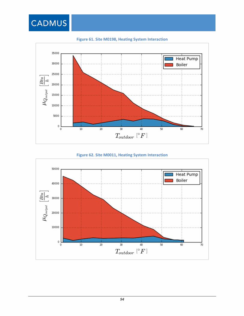
94



95

Unit Sizing For each indoor head, the evaluation team calculated the design’s heat gain and heat loss using ANSI’s

Manual J: Residential Load Calculation (Eighth Edition). Figure 63 shows the range of calculated heating

and cooling load for each space served. In general, the calculated heat load was 5,000 to 10,000 BTU/h

at 6 °F, and the median calculated cooling load was 5,000 BTU/h with a relatively tight range. Given that

most DMSHP heads have rated capacities of 9,000 BTU/h and greater, these plots seem to indicate that

DMSHPs were sized larger than necessary for cooling. As discussed later, this may be because they were

sized to meet heating needs. Fully half of all systems have heating loads above 10,000 BTUh at 6 °F, and

25% have loads great than 13,000 BTUh. These loads will be roughly 20% higher at ‐5°F, assuming a

balance point of 65 °F), or 12,000 and 16,000 respectively.

Figure 64 shows the ratio of rated unit capacity to calculated thermal load. This ratio was slightly above

100% for heating and just above 200% for cooling. As noted, the heating ratio probably was exaggerated

as heat loss was calculated at a design temperature of 6F, while units were rated at 17°F. That is the

median is likely below 100% of needs at colder temperatures as discussed below. Even at 17°F, nearly

half of the units were undersized for the space’s heating needs. The ratings of units’ heating capacity at

5°F are not standardized, with methods varying by manufacturer and AHRI ratings limited to 17°F.

The efficiency of a unit drops as the outside temperature drops, but capacity is dependent on airflow

and compressor speed. Some manufacturers report a flat capacity from 17°F to 5°F. Lacking

standardized metrics at colder temperatures, to roughly estimate how much capacity might drop from

17°F to 5°F, the evaluation team took a ratio of the two ratings for fixed airflow, using manufacturer’s

engineering data, and found about a 20% drop. Increased compressor speeds and higher airflows could

make up for this but that would be hard to determine without testing. Very roughly, if the median

capacity at 17°F was 110%, and if it dropped by 20%, the capacity would be as low 88% at 5°F. Even

without this drop, some 50% of units did not meet the heating load at temperatures below 17°F.

Conversely, the cooling ratio was slightly higher than indicated as the capacity was rated at 95°F, while

the heat gain was calculated at 86°F. Because DMSHPs have variable speed compressors and variable

speed fans, the evaluation team does not think that oversizing for cooling will appreciably affect savings

or efficiency.

96

Figure 63. Calculated Thermal Loads of Spaces Served by DMSHPs, N=141

Figure 64. Ratio of DMSHP Rated Capacity to Calculated Thermal Load of Spaces Served, N=140

97

Figure 65. Ratio of DMSHP Rated Capacity to Floor Area of Spaces Served

Figure 66 presents the ratio of rated unit capacity to the calculated design heat load; values greater than

one indicate the unit has more capacity than the calculated load for the space served with the caveats

discussed above. Table 19 summarizes these data. The team used the unit’s nominal capacity for these

calculations, calculating the design loads using a set of outdoor design conditions, set forth by ANSI in

Manual J. For Framingham, Massachusetts, this calculation results in outdoor ambient conditions of 86

°F during the summer and 6 °F during the winter.

Systems that could be characterized as outliers (i.e., capacity at greater than a 4:1 ratio to heat loss or

heat gain) resulted from installation of indoor units in spaces with only a small amount of area adjacent

to the exterior, such as hallways. In these cases, the heating and cooling likely spilled over and served

adjacent areas.

98

Figure 66. Heating and Cooling Rated Capacities Normalized by Calculated Design Loads

Table 19. Heating and Cooling Capacities, N=137

Heating Capacity

Ratio (Rating /

Design)

Cooling Capacity

Ratio (Rating /

Design [86°F])

Floor Area Served /

Cooling Capacity

(s.f. / ton)

Heating Capacity /

Floor Area Served

(BTU/h per s.f.)

Minimum 64% 96% 104 11

Maximum 1,129 115

Average See above 262% 333 36

Median 110% (17°F) 210%

The evaluation team received only a handful of complaints from homeowners, who regarded their units

as undersized to meet their cooling loads in summer; more common were complaints regarding

insufficient heat during the winter. The previous discussion supports this observation.

Figure 67 presents a scatter‐plot of rated capacities and calculated (Manual J) capacities, mapped as a

function of floor area served. Based on the characteristics of homes participating in the evaluation and

the resulting calculations completed via Manual J, the evaluation team considers it unlikely that

contractors use Manual J to size DMSHP systems. Based on these data, it also remains unlikely that

contractors use a “rule of thumb” to size a unit’s capacity to the floor area. As shown in Figure 67, none

99

of the data exhibit a good trend fit or strong correlation (as the R2 values are low relative to an ideal fit

of 1.0).

Figure 67. Relationship Between Design Cooling, Design Heating, and Rated Capacities as a Function of Floor Area Served

To test for use of rules‐of‐thumb, the evaluation team calculated the average floor area (in square feet)

served per ton of capacity for cooling and the BTUh per square foot supplied for heating. The result

averaged 333 sq. ft. per ton of cooling capacity, and 36 Btu/h per sq. ft. of floor area.

Finally, as shown in Figure 68, the team calculated the total rated cooling and heating capacity per total

floor area of each home, which included both DMSHPs and alternative heating or cooling systems. This

calculation examined the approximate portion of design capacity contributed by DMSHPs.

The figure shows the capacity of each HVAC system in the home, normalized by the home’s total floor

area. For most homeowners, a DMSHP system served as their only cooling source. Of homes in the

study, only eight had cooling capacities greater than 20 Btu/h per total s.f. of the home (or roughly 600

s.f./ton). The average cooling capacity was about 11.5 Btu/h per total s.f. of the home (or roughly 1,043

s.f. of home/ton). This is a far lower installed capacity than most central air conditioners (CAC) that

Cadmus has observed during other studies. This means that while the capacity of the DMSHP is far

100

greater than the cooling needs of the immediate space served, the overall installed cooling capacity of

DMSHP homes is far lower than homes cooled by a CAC. For heating, the average installed capacity was

67 Btu/h per s.f., where DMSHP accounted for 9.5 Btu/h per s.f. of that value.

Because DMSHP systems only accounted, on average, for about 14% of the total installed heating

capacity, one can reasonably consider these units secondary or spot‐heating solutions, with the bulk of

home heating performed by an alternative system or systems. About 7% of homeowners in Figure 68

used their DMSHP systems in conjunction with window air conditioning units; often to meet needs in

their home’s represented central areas (which would otherwise require multiple window units for

cooling). About 8% of homeowners used the system in conjunction with central air conditioners,

presumably because the DMSHPs allowed homeowners more control over individual set points within

their homes. Homeowners also indicated that DMSHPs helped to condition areas added to homes after

original construction and only served partially by the existing systems.

Figure 68. Normalized HVAC System Capacities

101

Behavior Influence At the beginning of winter 2016, the evaluation team distributed a postcard to a small group of study

participants. All participants had existing, operational electric resistance heat in the same room as their

newer DMSHP. The postcard was intended to encourage changes in operating behaviors by

homeowners and to promote more efficient operations of the coincident systems. Figure 69 presents

the postcard’s primary content.

Figure 69. Behavior Influence Postcard

Figure 70 presents compares behavior for these participants from winter 2015 to winter 2016. After

normalizing for different weather conditions between the two winters, it appears this postcard mailing

had the intended effect, and DMSHP usage increased among recipients. This finding indicates some

potential exists for behavior‐influence efforts to increase the efficiency of customer operating

behaviors.

102

Figure 70. DMSHP Usage for Behavior Influence Postcard Recipients

Additional Findings Throughout the study, the field team had multiple opportunities to speak with homeowners and learn

about their experiences in purchasing and installing DMSHPs. The team observed a range of situations

where homeowners noted diminished performance and sought guidance from field staff on improving

their units’ operation.

Filter Cleanliness

Staff observed the cleanliness of filters and rated them from one to three, noting whether they were

clean (1), moderately dirty (2), or very dirty (3), respectively. The average filter received a rating of 1.5 to

1.6, indicating that filters typically fell between clean and moderately dirty. Dirty filters more often

occurred alongside the following conditions (in descending order of influence):

Pets in the home

Wood or wood‐pellet stoves used as a heat source

Homeowner was unaware of the filter’s presence

Homeowner was unable to reach the filter for cleaning

As shown in Figure 71, filters can be checked for cleanliness visually. In this extreme case, dust

accumulation on the filter hindered the fan’s full‐speed volume by 69%. Filters can be cleaned with a

household vacuum or in a sink, leaving the filter to air dry before reinstalling.

The evaluation team examined filter cleanliness’ impacts of on fan performance and air volumes. Under

laboratory and field conditions, the team tested units under “as‐is” filter conditions, without a filter,

103

with a clean filter, and using an apparatus to simulate a dirty filter. The testing results indicated a filter’s

cleanliness changed the operating point along the “fan current vs. air volume” curve, but even a very

dirty filter shifted the curve down by less than 10% versus a cleaned filter and by about 5% versus an

average filter. Based on these data, the team concluded that no adjustments to account for filter

cleanliness were necessary when processing measured data, since the measurement approach (i.e.,

logging indoor head current) accurately represented the unit’s delivered airflow.

Figure 71. Filter Maintenance

Outdoor Unit Placement

The field staff observed many DMSHP outdoor units improperly mounted or lacking appropriate

clearances from roof drain water. During the winter, many units were exposed to snowmelt from a

home’s roof or to water collected from the defrost cycle (as melted snow and ice can build up on the

unit itself). Without adequate clearance below the unit, this water could freeze and impair condenser

fan operation. The team observed this scenario for at least one site, illustrated by Figure 72. The

manufacturer’s recommended clearance illustration43 does not clearly define a minimum clearance

value above the ground, but it implies that mounting the unit on two cement blocks would be

appropriate. While the unit in the photo (left) has about one inch of clearance, the illustration (right)

implies a unit should have about four inches of clearance below the unit.

43 Mitsubishi Electric Corporation. Outdoor Unit Service Manual No. OBH543 Revised Edition‐A. September 2010.

Available online: http://www.mitsubishipro.com/media/214712/muz‐fe09‐18na_service_obh543a_9‐10.pdf

104

Figure 72. Clearances Underneath Outdoor Units

Clearance issues do not exclusively result from installation practices. Several homeowners reported

experiencing rapidly diminishing capacity over time, and field staff found outdoor units within piles of

items or other debris. In one notable case, shown in Figure 73, a pile of lawn furniture encircled an

outdoor unit, which was half‐protected from scratches by a tarp.

105

Figure 73. Clearances Around Outdoor Units

The effort required to maintain a DMSHP outdoor unit’s operable condition during winter presents

another anecdotal finding. As this study stretched across the winter months, particularly January and

February of 2015 (which experienced extended freezing temperatures and uncommonly high snowfall),

several participants’ DMSHP outdoor units became encased in snow and/or ice. Figure 74 shows a

DMSHP unit that the evaluation team visited in February 2015. Without clearance around the outdoor

unit, the DMSHP could not provide heating to the home’s interior. The team removed snow from the

front and rear of the unit, using only their hands to prevent damage to the exposed heat exchanger fins

or the refrigerant lines.

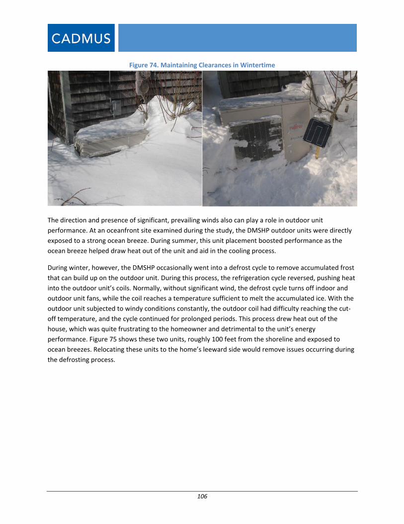
106

Figure 74. Maintaining Clearances in Wintertime

The direction and presence of significant, prevailing winds also can play a role in outdoor unit

performance. At an oceanfront site examined during the study, the DMSHP outdoor units were directly

exposed to a strong ocean breeze. During summer, this unit placement boosted performance as the

ocean breeze helped draw heat out of the unit and aid in the cooling process.

During winter, however, the DMSHP occasionally went into a defrost cycle to remove accumulated frost

that can build up on the outdoor unit. During this process, the refrigeration cycle reversed, pushing heat

into the outdoor unit’s coils. Normally, without significant wind, the defrost cycle turns off indoor and

outdoor unit fans, while the coil reaches a temperature sufficient to melt the accumulated ice. With the

outdoor unit subjected to windy conditions constantly, the outdoor coil had difficulty reaching the cut‐

off temperature, and the cycle continued for prolonged periods. This process drew heat out of the

house, which was quite frustrating to the homeowner and detrimental to the unit’s energy

performance. Figure 75 shows these two units, roughly 100 feet from the shoreline and exposed to

ocean breezes. Relocating these units to the home’s leeward side would remove issues occurring during

the defrosting process.

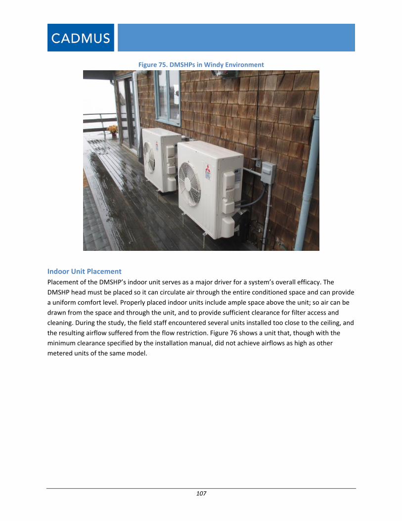
107

Figure 75. DMSHPs in Windy Environment

Indoor Unit Placement

Placement of the DMSHP’s indoor unit serves as a major driver for a system’s overall efficacy. The

DMSHP head must be placed so it can circulate air through the entire conditioned space and can provide

a uniform comfort level. Properly placed indoor units include ample space above the unit; so air can be

drawn from the space and through the unit, and to provide sufficient clearance for filter access and

cleaning. During the study, the field staff encountered several units installed too close to the ceiling, and

the resulting airflow suffered from the flow restriction. Figure 76 shows a unit that, though with the

minimum clearance specified by the installation manual, did not achieve airflows as high as other

metered units of the same model.

108

Figure 76. Vertical Clearance on Indoor Unit

Unit Controls

During the study, field staff continually encountered homeowners confused by the operation of the

DMSHP remote. Generally, many homeowners found images on the remote too small to read and too

similar to each other to understand. These homeowners reported a lack of clarity when using the

remote resulted in several service calls to installers for nonoperational units that, ultimately, were

resolved by adjustments of the remote settings.

As shown in Figure 7744 (inside the red box), the symbols for cooling (symbol 2 from the top) and heating

(symbol 4 from the top) look very similar, especially given the remote’s actual size (one‐half the size of

the image shown in the figure). During a visit by the evaluation team, the homeowner sat in a 92 °F

house with the DMSHP set to heat, believing it was set to cool.

44 Mitsubishi Electric Corporation. Indoor Unit Service Manual No. OBH542 Revised Edition‐A. September 2010.

Available online: https://www.rfwel.com/downloads/manuals/KMO8C‐User‐Manual.pdf

109

Figure 77. Operation of DMSHP Remote Control

Staging of Alternative Heating Systems

Homeowners frequently asked the evaluation team about interactions between two or more forms of

heat within a home. Specifically, homeowners wanted to know when to use each system and how to set

the thermostats for each (i.e., “staging”). Based on data the team collected and subsequent analysis, the

team determined that using the DMSHP proved more cost‐effective at milder heating temperatures.

As the COP of DMSHP units decrease with outdoor temperatures, the price of each heat unit increases.

This stands in contrast to fossil‐fuel heating systems, which typically draw combustion air from a semi‐

conditioned space and produce the same amount of heat across a wide band of temperatures. As one

system becomes more expensive to generate heat and the other stays constant, a crossover point

occurs where a fossil‐fuel heating system becomes the more cost‐effective heating method. This

crossover point depends on each heating system’s efficiency, the fuel’s cost, and the fuel’s heat content.

To illustrate this concept, the COP chart in Figure 52 can be used as a reference. On average, because

DMSHP units exceeded a COP of 1.0 at all temperatures, a DMSHP proved a more efficient use of energy

than an electric resistance heater.

The crossover point, defined as the point where using either source proves is equally cost‐effective, is

characterized by the following equation:

$

$

110

Generally, the price per unit of energy is written as follows:

$

/

Evaluating this in terms of BTUs and for the DMSHP, this becomes:

$ $∗

1

3,412∗

1

Where:

COP is related to temperature through Figure 52 and Figure 53 $

= price of one kWh of electrical

energy. For an oil boiler, this equation is written as follows: $ $

GallonofOil∗

139,600∗

1

Where:

$

= price of one gallon of #2 heating oil

= the boiler’s efficiency

For a gas furnace, this equation is written as:

$ $

∗

1,050∗

1

Where:

$

= price of one therm of natural gas

= the furnace’s efficiency

Figure 78 shows a two‐dimensional map of electric and fuels prices. The topographical style lines show a

third dimension of the temperature breakpoint discussed above, where a DMSHP becomes less

expensive to operate than an alternative fuel‐fired heating system. The temperature dependence results

from DMSHPs’ drop in efficiency at lower temperatures. A round blue circle indicates average energy

prices for winter 2016; a red triangle indicates energy pricing for winter 2015.

For natural gas, the figure shows a temperature breakpoint above 70°F for either winter, meaning a

DMSHP only operates cost‐effectively above 70°F (compared with an 80% efficient heating system).45

45 System efficiency is inclusive of duct losses, and furnace fan and boiler pump energy use. It is, however, lower

than the rated or measured combustion efficiency.

111

This effectively means a DMSHP does not provide a viable direct replacement for a gas‐fired system at

today’s energy prices. This analysis does not account for zonal savings. For example, if a homeowner

used a DMSHP to heat 30% less of their home, that temperature balance point would drop to 50°F.

The figure also shows a temperature balance point about 32°F for an oil‐fired system in 2016 and 12°F in

2015. The balance point for propane was ‐15°F for both winters, meaning the DMSHP always was less

expensive than the propane option.

Figure 79 shows the same analysis, but for units listed as cold climate units. These units operate

somewhat more efficiently, and the economic balance points shift to colder temperatures, where gas

balance points were above 58°F for both winters. Balance points were 26°F for an oil‐fired system in

2016 and 8°F in 2015. These values do not account for zonal savings. For example, if a homeowner can

use a DMSHP to heat 30% less of their home, the temperature balance point would drop by 20°F

or more.

Figure 80 shows the same analysis, but bases it on the rating curve of a current cold‐climate unit, with

an HSPF of 13. A DMSHP operates more economically than propane for all temperatures; so it is not

shown in this figure. The balance point for oil dropped slightly, about 15°F in 2016 and 8°F in 2015. The

balance point for natural gas dropped to 40°F for 2015 and 28°F for 2016.

112

Figure 78. Operational Break Point Temperature of Heating with DMSHP, Winter 2016, All Units

113

Figure 79. Operational Break Point Temperature of Heating with DMSHP, Winter 2016, Cold Climate Units

114

Figure 80. Operational Break Point Temperature of Heating with DMSHP, Assumed HSPF of 13

115

At outdoor temperatures above the crossover point and where zoning allows, the evaluation team

recommends setting the DMSHP thermostat to the desired temperature and setting the boiler/furnace

zone thermostat several degrees below. When the outdoor temperature drops below the crossover

point, the relationship of the two systems should switch. The boiler/furnace should then be set at the

desired temperature, and the DMSHP should be set several degrees below. In both cases, the system set

to the lower temperature will act as a backup should the primary system not maintain the desired

temperature.

When setting the DMSHP as the primary system, a risk exists: it is possible that sections of pipe for the

boiler and radiators could freeze if on the outer walls of a home or if air infiltration occurs near a pipe. If

possible, circulating water within the pipes can be helpful at low outdoor temperatures to avoid

freezing. Alternatively, utilizing the boiler intermittently at low outdoor temperatures will help avoid

frozen pipes.

Localized Heating

The field team identified another potential savings source by interviewing participants about their

heating behaviors. Several participants responded that they often used the DMSHP to heat a small

section of the home, while leaving central heat at a lower set point. For homes without zone control

(i.e., just one central thermostat), this approach creates energy savings.

When operating the DMSHP in this way, interactions with central heating should be considered,

especially at the thermostat’s location. For example, if the DMSHP heats the section of a house where

the thermostat controlling a central heating boiler is located, that thermostat may never call for heat as

the DMSHP satisfies its requirement. In this scenario, the home outside the DMSHP area grows cold as

DMSHP heat will not reach these areas, and the boiler will not provide heat as its control senses a space

controlled properly above its set point.

Non‐Energy Benefits

Although non‐energy benefits can be difficult to quantify, they can provide insights into consumer

behaviors. During the study, the evaluation team learned of many non‐energy benefits that customers

reported from their experiences. Largely, these benefits divided into two subgroups, based on

equipment displaced by the DMSHP:

For customers replacing window air conditioners, non‐energy benefits included the following:

Use of operable windows for ventilation and daylighting

Increased control over indoor air temperatures and humidity

Increased uniformity in air temperatures throughout a served space

Increased security from locking windows

Increased auditory comfort from compressors isolated away from the house framing

Quieter operation of indoor air fans

Isolation of outside noises from closed windows

116

Decreased exposure to outdoor allergens

Additional heating available, if needed

Decreases in personal and property risk from installations or removals of window air

conditioners

Increased safety from decreased indoor outlet electrical draws

Customers who purchased DMSHPs rather than centralized cooling systems reported the

following non‐energy benefits:

Increased control of localized cooling

Easier installation experiences (as ductwork was not needed)

Heating and cooling provided by a single technology

Multiple units decreasing the mean time to total failure for the entire HVAC system

Lower installed costs if a cooling system served only a portion of the home

117

Discussion

In general, the evaluation found DMSHPs operated in highly variable ways, resulting in widely varying

hours of use, energy consumption, and energy savings among units. Some variation results from a

variable speed design, but a larger factor appears to be how users operate their equipment. A discussion

follows that addresses results from cooling, heating, efficiency ratings, and airflow.

Cooling The evaluation identified an average EFLH cooling value of 218 hours, well below the value of 360 hours

assumed in the Massachusetts and Rhode Island TRMs. Units often operated at low capacity, or

customers turned them off for periods. The following elements contributed to the low EFLH:

Units sometimes operated in dehumidifier or “dry” mode, where users could not increase or

decrease set temperatures. In dry mode, the indoor unit senses the indoor ambient

temperature, and lowers the coil temperature a few degrees to induce condensation formation.

The unit then operates the fan on the lowest speed setting to avoid decreasing the space

temperature too much.

Some units cooled seldom‐used spaces and were turned on only when needed.

As DMSHP units did not experience duct losses or suffer from insufficient evaporator airflow (as

some central air conditioning units might), they provided the same cooling level with fewer

EFLH. That is, a central air conditioner can lose efficiency at the air handler due to low airflow,

and then lose more energy through duct leakage and heat losses/gains as ducts pass through

unoccupied spaces. DMSHPs did not experience these losses.

On average, units were sized to provide about 2.6 times the design‐cooling load calculated using

Manual J. This could result from contractors sizing DSMHP units to meet larger design‐heating

loads. Units also may be designed to cool adjacent spaces when doors to a cooled room remain

open.

TRM sources for the legacy EFLH values may be inappropriate for DMSHPs (i.e., the cooling EFLH

value was based on a 2009 study of central air conditioners).

The top 25th percentile units had EFLHs that were very close to and in some seasons, above the

TRM values, showing a good portion of units were used more heavily.

Given these factors, it is not entirely surprising that the average EFLH fell below TRM values. Savings

calculations in the Massachusetts and Rhode Island TRMs are a function of this EFLH parameter, but also

of unit capacity. A low EFLH reduces savings in a TRM equation, but it may not mean reduced savings in

in relation to a smaller unit that would have higher EFLH. For example, if a unit’s size were reduced by

50%, the EFLH would roughly double, but the TRM equation would yield the same savings:

2 (EFLH)* 0.5 (Capacity) = EFLH * Capacity

118

The evaluation team based savings on the baseline and efficient systems providing identical cooling but

at varying efficiencies (i.e., a 16 SEER air conditioner can deliver cooling using 75% of the energy

required for a12 SEER air conditioner).

In many cases, DMSHPs provide additional savings beyond more efficient operation, and therefore may

provide higher savings than indicated through comparisons with baselines. As shown later in this report,

DMSHPs were installed at approximately 1 ton of capacity per 1,043 s.f. of home floor area, a value far

lower than typically observed for central air conditioners. Homeowners frequently shut off DMSHPs due

to unoccupied rooms or mild outdoor temperatures. Thereby, a DMSHP can deliver zonal savings by

performing less cooling. DMSHP also can run in dehumidification mode, further reducing the need for

cooling.

When considering new construction program, DMSHPs could potentially deliver savings from zonal

behaviors where homeowners fully cools only a portion of their house, while central air conditioners

typically do not offer this control—to cool one room, the homeowner must cool their entire house.

For this study, the majority of DMSHPs served as the only cooling source. Homes cooled solely with

DMSHPs used an average of 194 kWh for the cooling season, including standby power. Using the

Massachusetts TRM value for a central air conditioner’s EFLH (360 hours), a home would use

approximately 830 kWh/season for a 2.5‐ton unit, and about 1,000 kWh/ season for a 3‐ton unit. This

striking difference (830 – 1,000 kWh vs. 194 kWh) argues for investigating marketing and incentivizing

DMSHP units as an alternative to central air conditioners in new construction.

Heating The study found an EFLH heating value of roughly 450 hours. In nearly all cases, observed DMSHP units

provided heat coincidentally with other systems. In most cases, DMSHPs served as secondary systems,

either to provide heat for a single space or to provide heat above a primary system’s base load.

The cost‐effectiveness of DMSHPs used for heating depends on alternative heating systems, energy

prices for a given period, and outside air temperatures. Compared against electrical resistance and

propane heating, DMSHPs proved more cost‐effective for all energy prices (using the same energy

source) and all outdoor air temperatures. For oil‐fired systems, the relative energy price determines the

temperature above which a DMSHP became more cost‐effective. Given low current oil prices, relative to

historic values, DMSHPs offer cost‐effective heating when compared to oil but only for temperature

ranges discussed in this report. A DMSHP, however, seldom proved cost‐effective when compared to

natural gas heating systems (excepting a scenario where a DMSHP heats single space, thus negating the

need to turn on a whole house heating system).

COP/SEER/HSPF The evaluation team directly metered efficiencies of DMSHP units during winter and summer seasons.

Most previous studies have estimated COP using metered power (i.e., not very accurate), or have

calculated COPs for brief periods and small unit quantities. This study found unit efficiencies varied

119

widely by site and period to period, partly due to temperatures and partly due to set points. Field‐

measured seasonal efficiencies for most units fell below their rated values, on average, although some

units met or exceeded their ratings. Measured SEER values below unit ratings occurred for the

following reasons:

Some seldom‐used units still used some standby power.

Some homeowners used DMSHPs only used to cool on the hottest days; so their cooling

efficiency was closer to rated EER values (i.e., the efficiency rating at 95 °F) than to SEER values.

SEER and EER tests run under specific conditions might not fully represent actual operations. For

example, the SEER test uses return air is 80 °F—a temperature much higher than most homes

during the cooling season.

Units used for other functions could reduce a units rated performance (e.g., fan‐only mode, dry

or dehumidification mode).

Measured HSPF values could fall below rated values for the following reasons:

Some homeowners used DMSHPs during very cold outdoor conditions, when the resulting

DMSHP COP fell below its rated value.

HSPF tests run at specific conditions may not fully represent actual operations.

Units used for other functions could reduce rated performance (e.g., fan‐only mode).

Site conditions could cause units to run in defrost mode for long periods of time, decreasing

efficiency. The evaluation team has completed other studies that discovered marked differences

in the frequency of defrost cycles for different brands.

Although field‐measured efficiencies generally fell below rated efficiencies, this does not mean that

manufacturers have not been forthright. Others including AHRI stipulate test procedures for cooling and

heating at 47°F and 17°F. Many manufacturers use third‐party laboratories for testing, so values are

verified. A number of units performed at their ratings, supporting the contention that operating

conditions and operators’ behaviors greatly contribute to delivered efficiencies.

This study metered units with a rated average 20.6 SEER and a rated average 10.3 HSPF. Manufacturers

continue to increase the efficiency ratings of systems they offer, with the upper range of units currently

offered at 33 SEER, with many units above 25 SEER. DMSHP manufacturers offer units with HSPF ratings

up to 14, with many units above 12 HSPF. These new units would deliver cooling and heating more

efficiently than units measured for the study.

Savings Values EFLH and savings values are based on averages that included lightly used equipment as well as on

equipment with rated efficiencies below that currently available in the marketplace. While current EFLH

and savings values may be low relative to legacy TRM values, the evaluation team has observed high

120

heating usage and EFLH in northern New England by populations motivated to displace oil heat.46 As

outlined in the recommendations section, the team recommends incentivizing the highest‐tier efficiency

levels to increase savings, and combining incentives with contractor and consumer education. This

approach could target high‐use customers found in this study’s customer distributions.

Controls and Zoning Use of preexisting heating systems limit DMSHP use for heating. Most furnaces are single‐zone systems,

meaning a single thermostat and single set point controls the home’s temperature. In these homes, if a

DMSHP heats only one or two rooms, homeowners find it difficult to use the DMSHP as a primary

heating system because if the rely solely on the DMSHP, other portions of the house remain

unconditioned. If they turn on the baseline system to heat the rest of the house, the area served by the

DMSHP is also heated. A similar issue occurs with boiler‐heated homes, but might be more solvable as

boilers often heat separate zones, served by separate zone valves or separate secondary pumps. In

homes with individually controlled electric strip heating, the primary system can be more readily

replaced with a DMSHP.

To increase DMSHP heating use and associated savings, the zone served by the DMSHP needs to match

a zone of the primary system. This can be accomplished by targeting homes with zoned (e.g., oil or

propane‐fired) boilers, room controlled electrical resistance heating, or by installing multi‐head systems

that combine to serve a complete zone. The DMSHP’s temperature setting would then be set above the

dead band of the primary system’s thermostat (i.e., 3°F). For example, if the DMSHP were set to 70°F,

the primary system’s thermostat would be set to 67°F.

Allowing the DMSHP and the primary thermostat to communicate with each other would improve this

situation. Under this scenario, set points for the primary and DMSHP would be 67°F and 70°F,

respectively. When the room became unoccupied, the set points could drop to lower temperatures. This

way, the DMSHP would become the primary heating system, and additional zonal savings could be

achieved where unused portions of the home were not fully heated.

Achieving this communication, however, currently remains a challenge. Major ductless system

manufacturers and wireless thermostats makers recently have made progress in designing systems that

work together. The evaluation team recommends makers of various smart thermostats and DMSHP

manufacturers continue collaborating to develop protocols that allow the devices to communicate.

Airflow Generally, airflow measuring airflow is difficult due to its variable nature, and most methods present

large associated uncertainties. Compounding this, measuring a DMSHP’s airflow is even more difficult as

the airflow is free discharge (i.e., not ducted) and variable, with most indoor heads capable of four or

46 Unpublished Cadmus study on Vermont.

121

more speeds. This evaluation reviewed the most current methods for measuring DMSHP airflow (e.g.,

fan amperage, volumetric) spot measurements and added some notable improvements.

The evaluation team measured a large number of models and units, which decreased uncertainty. The

team constructed and employed a quasi‐laboratory flow nozzle to check measurements of a field‐

practical balometer. The testing found airflows 10% less than the units’ rated values generated by

independent laboratories. That these field‐measured airflows are close to rated values makes sense;

unlike central‐ducted systems, DMSHP units installed in homes generally are similar to those installed on

the wall of a test facility (i.e., no ducts or obstructions to modify airflow).

Uncertainly exists regarding these and any airflow measurements. For five test homes, the evaluation

team deployed the powered, quasi‐laboratory flow nozzle and the balometer. For these homes at all

indoor fan speeds, the balometer measured airflow similar to but 5% to 10% higher than the flow

nozzle. As no compelling evidence emerged to support one method as more accurate than another, the

team used the balometer readings without adjustment. This judgment did not affect DMSHP savings

estimates, as baseline system efficiencies were decremented by an equivalent amount, along with

proposed DMSHP systems (see Analysis: Savings section).

122

Recommendations

Recommendations

Program

Recommendation: The evaluation team recommends exploring ways to improve the PAs’ existing lost

opportunity program for DMSHPs, such as how best to encourage the installation of multiple DMSHP

heads to better match existing zones and displace primary system operation. Although the EFLHs

decreased from the values prescribed in the Massachusetts TRM, the study still finds that a modest level

of savings are achievable by moving from a standard efficiency DMSHP to a higher efficiency DMSHP.

Substantially more savings could be achieved (i.e., the top 25% of savings) if newly installed DMSHPs are

operated more regularly and continuously by better matching and integrating them zonally with primary

heating systems, through better configuration design and installation and contractor and customer

education and training. For example, contractors would focus their design efforts on specifying the

appropriate number and size of DMSHP heads to match and heat entire zone(s) rather than a single

room. Customers would then be educated on how to properly set the set points for both their primary

and DMSHP heating systems, which will depend on their primary fuel type and outdoor temperatures.

Finally, establishing program incentives for the generally more efficient, cold climate heat pumps would

lead to increased program savings.

Recommendation: The evaluation team recommends exploring methods for targeting homes with

electric resistance heating for DMSHP retrofits. DMSHPs will nearly always be less expensive to operate

than electric resistance heat, as shown by the COP of DMSHPs remaining above 1.0 on average for

nearly all outdoor temperatures. Even at very cold temperatures where some non‐cold climate units

approach a COP of 1.0, the number of hours in this condition are very few. Prior to new activities,

program and consumer cost‐effectiveness would require review.

Recommendation: The team recommends targeting propane‐heated homes for DMSHPs. As

Figure ES‐6 and Figure ES‐7 show DMSHPs always operate less expensively than propane heating

systems. Prior to new activities, program and consumer cost‐effectiveness and regulatory considerations

for fuel switching would require review.

Recommendation: The team recommends exploring methods for addressing oil‐heated homes. To

target these homes, homeowners should be educated to turn off a DMSHP during very cold outdoor

conditions (below 8°F in 2015 and below 25°F in 2016), when an oil‐fired system would operate less

expensively (depending on energy prices and cold temperature COPs). This operating scheme, however,

may not appeal to all customer types, as many may not wish to concern themselves about which heating

system to operate and when. If oil prices increase against electric energy rates, the switchover

temperature point for oil to DMSHP heat may move lower, allowing continual use of a DMSHP.

Switchover points for all fuel comparisons will decrease as more efficient DMSHP units become

123

available. Prior to new activities, program and consumer cost‐effectiveness and regulatory

considerations for fuel switching would require review.

Recommendation: Based on large energy‐usage differences in DMSHP‐cooled homes and central air

conditioner‐cooled homes, the team recommends examining opportunities for a new construction

measure to substitute DMSHPs for central air conditioners.

Future Studies

This study provided a great deal of data describing how DMSHPs actually operate in Massachusetts and

Rhode Island homes. These operations varied widely among units, with some used heavily and others

used more like appliances turned on for short periods. Highest savings could be achieved by targeting

homes where such units would deliver greater amounts of heating and cooling (i.e., where they can be

installed to match the zoning of existing systems).

Another factor in increasing DMSHP savings will be development of controls that allow ductless systems

and primary thermostats to interact and share information. The evaluation team recommends either

targeting studies for new construction homes without natural gas available and where central air

conditioning systems would be installed; or existing homes with electrical resistance and propane

heating. These studies would help refine the best ways for DMSHP programs to achieve maximum

savings.

Other future studies could explore the use of interfaces between learning thermostats and ductless

systems. Future research questions include the following:

How can utilities target homes with a high probability of using DMSHPs to displace more heating

and cooling, therefore producing higher savings?

What potential exists for new high‐HSPF units to displace heating?

What optimal zonal and control characteristics maximize use of DMSHPs?

For new construction, how large would zonal savings have to be to avoid installations of single‐

zone central systems?

124

Appendix A: Measuring Airflow in DMSHPs

Airflow Appendix A may repeat certain report elements, but the evaluation team chose to provide additional

detail on methods used for establishing DMSHP airflow. The team hopes that the following discussion

will help inform future field studies regarding best practices for estimating airflow, especially for

extended‐duration conditions.

The evaluation team recommends the following the airflow measurement methods developed in

previous published studies and refined through this study:

1. Use either a balometer or a powered flow hood for measuring volumetric airflow coincidently

with measured fan amperage. For large studies, a non‐powered flow hood or a powered

balometer (for low flows)—such as a Flow Blaster—would be practical.

2. The team does not recommend using a flexible flow bag for airflow measurement, as applied in

other studies.

3. A flow nozzle, such as the one tested in this study, can be used for small‐scale, controlled, or

laboratory studies, but it is not recommended for large‐scale field studies. It does, however,

prove useful for calibrating or adjusting the measurements of equipment recommended in #1.

Motivation and Intention

The concluding equation presented in the Method/Energy section defines energy removed or added to

air as a direct function of the volumetric air flow ( ). To determine that volumetric air flow, the

evaluation team used a combination of on‐site point measurements and logged values. The team chose

these methods for their ease of implementation, lack of interference with unit operations, quality of

data collection, and preservation of unit integrity and housing.

Background Literature for Flow Hoods

At the project’s beginning, the evaluation team reviewed publicly available literature, seeking to

understand the existing body of knowledge and to check the proposed approach for measuring

volumetric air flow against other methods. In November 2012, a Lawrence Berkeley National Laboratory

(LBNL) publication proposed a variety of methods for taking such measurements, and presented seven

methods of measuring air flow using flow hoods against a laboratory metric.47

Typically, flow hoods are composed of fabric stretched over a collapsible, rigid frame that guides the air

flow over a velocity or pressure‐sensing element. Commercially produced, these units are frequently

47 J. Chris Stratton, W.J.N Turner, Craig P. Wray, Iain S. Walker. Measuring Residential Ventilation System

Airflows: Part 1 – Laboratory Evaluation of Airflow Meter Devices. LBNL‐5983E. Ernest Orlando Lawrence

Berkeley National Laboratory. November 2012. Available online: <https://buildings.lbl.gov/sites/all/files/lbnl‐

5983e.pdf>.

125

used in the air‐balancing industry. Flow hoods can be divided into two categories—powered or non‐

powered—with the 2012 LBNL study testing a representative sample of 366 and 369 hoods,

respectively.

The November 2012 LBNL publication cited an earlier 2001 LBNL publication that clarified the division of

flow hoods. The 2001 publication divided standard flow hoods among two examined categories (i.e.,

active and non‐powered):48

Active (or powered) flow hoods reduce the effects of back pressure on flow measurements,

usually through use of an exhaust fan to draw static pressure within the flow hood to equal the

ambient environment.

Non‐powered flow hoods cannot forcefully remove the buildup of static pressure. To

compensate for this, these instruments typically employ a damper to evaluate the impact of

static pressure on the calculated flow and to produce a revised number, factory calibrated

against a standard.

Using powered/non‐powered segregation, the 2012 LBNL report concluded that two of the four non‐

powered flow hoods tested did not produce acceptable accuracy (defined at ±5 cfm or ±10% of the

measurement reading from the reference airflow). In contrast, all three powered flow hoods produced

acceptable accuracy.

On the surface, this conclusion helps reinforce decades‐old skepticism in the industry regarding the

accuracy of flow hoods for airflow measurement. Both the 2012 LBNL report and a separate 1999

publication, however, confirmed that flow hoods realistically provide the best method for measuring

airflow with adequate accuracy.49

Excerpted from LBNL‐5983E, Figure 81 shows a test for the model used in this study. The graph shows a

range of airflow, tested up to 220 CFM, or roughly the two lower speeds of the DMSHP metered in this

study. The boundary of accuracy is shown in green: at ±5 CFM for low flows and at ±10% for higher

flows, with y = 0 representing laboratory measurements taken as the true measurement.

48 Walker, I.S., C.P. Wray, D.J. Dickerhoff, and M.H. Sherman. Evaluation of Flow Hood Measurements for

Residential Register Flows. LBNL‐47382. Lawrence Berkeley National Laboratory. September 2010. Available

online: http://epb.lbl.gov/publications/pdf/lbnl‐47382.pdf

49 Ernest E. Choat, P.E. “Resolving Duct Leakage Claims.” ASHRAE Journal (March 1999). Accessed June 6, 2016.

Available online: http://search.proquest.com/openview/d6c7203563370c8a9e8e050b11f0b2a9/1?pq‐

origsite=gscholar

126

Figure 81. LBNL‐5983E Figure 14

At first glance, the balometer would appear inaccurate and imprecise, with varied readings outside of

the accuracy boundary. The figure presents, however, two types of data: inlet flows, which represent

typical use of a balometer; and the method used in this study, where air enters a wide mouth and flows

to a measurement area; and outlet flows, where the balometer is used in reverse. Filtering Figure 81 for

only inlet flows (black crosses) yields Figure 82, which shows TSI/Alnor EBT721 measurements within 5%

of the reference measurement above 80 CFM (few DMSHPs even have speeds below this flow rate).

As stated in the 2012 report and in personal communications with its lead author,50 the TSI/Alnor

EBT721 produces acceptable accuracy when used to measure inlet flows.

50 Personal communications with Dr. Iain Walker. Response to question via e‐mail regarding LBNL‐5983E

Publication. May 19, 2016.

127

Figure 82. LBNL‐5983E Figure 14, Adapted

This large difference in accuracy results from the design of the balometer itself. As shown in Figure 83,

during inlet flow, the air stream is guided towards the measurement section in the fabric cone. This

results in smoother (more laminar) flow. In contrast, during outlet flow, air abruptly enters the

measurement section and exits into the DMSHP. This does not smooth the airflow and consequently

lowers the measurement accuracy. Fortunately, this study only used balometers for the inlet mode.

Figure 83 show differences between inlet and outlet flows and assists in explaining data presented in

Figure 81.

Figure 83. Inlet vs. Outlet Flow

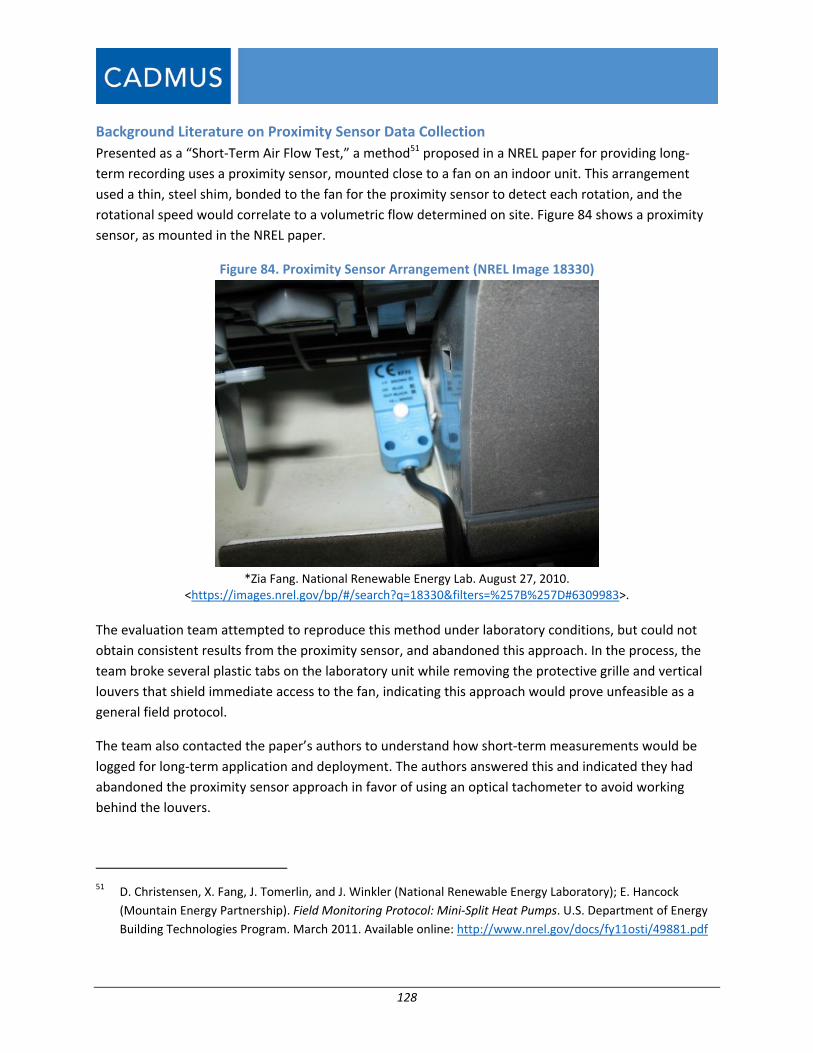
128

Background Literature on Proximity Sensor Data Collection

Presented as a “Short‐Term Air Flow Test,” a method51 proposed in a NREL paper for providing long‐

term recording uses a proximity sensor, mounted close to a fan on an indoor unit. This arrangement

used a thin, steel shim, bonded to the fan for the proximity sensor to detect each rotation, and the

rotational speed would correlate to a volumetric flow determined on site. Figure 84 shows a proximity

sensor, as mounted in the NREL paper.

Figure 84. Proximity Sensor Arrangement (NREL Image 18330)

*Zia Fang. National Renewable Energy Lab. August 27, 2010.

<https://images.nrel.gov/bp/#/search?q=18330&filters=%257B%257D#6309983>.

The evaluation team attempted to reproduce this method under laboratory conditions, but could not

obtain consistent results from the proximity sensor, and abandoned this approach. In the process, the

team broke several plastic tabs on the laboratory unit while removing the protective grille and vertical

louvers that shield immediate access to the fan, indicating this approach would prove unfeasible as a

general field protocol.

The team also contacted the paper’s authors to understand how short‐term measurements would be

logged for long‐term application and deployment. The authors answered this and indicated they had

abandoned the proximity sensor approach in favor of using an optical tachometer to avoid working

behind the louvers.

51 D. Christensen, X. Fang, J. Tomerlin, and J. Winkler (National Renewable Energy Laboratory); E. Hancock

(Mountain Energy Partnership). Field Monitoring Protocol: Mini‐Split Heat Pumps. U.S. Department of Energy

Building Technologies Program. March 2011. Available online: http://www.nrel.gov/docs/fy11osti/49881.pdf

129

Further, the authors reported that they recently achieved success by not measuring the fan speed at all;

rather, they used the fan current as a proxy for airflow—a method discussed in this appendix (see

Background Literature on Current Transformer Data Collection).52 The authors also referenced a more

recent study that used fan current as a proxy for airflow.53

Background Literature on Optical Tachometer Data Collection

As discussed, the NREL authors also employed an optical tachometer for measuring airflow. Very similar

to the proximity sensor method, this method uses a strip of reflective tape placed on the fan blades.

The evaluation team verified that this method generated values for a fan’s rotational speed, although

equipment available to the team would not allow long‐term concurrent readings of fan rotational

speeds and air volumes supplied by the unit. In addition, the team found that, to deploy an optical

sensor, the DMSHP head had to be disassembled. Due to the way some heads are constructed, this

would very likely damage many units.

Lastly, the team expressed concerns that installing a sensor close to a rotating fan could cause the

sensor wire to entangle the fan, in some cases leading to damage and customer dissatisfaction.

Consequently, this study did not rely upon optically sensing fan rotational speeds.

Figure 85 shows spot measurements conducted on the laboratory unit. Here, the vertical louvers and

protective grille were removed to ease access to the fan; these should be reinstalled to return the unit

to its proper condition.

52 Personal communication with Dane Christensen and Dr. Jon Winkler. Response to question via e‐mail

regarding field monitoring protocol MSHP. March 30, 2016.

53 Williamson, James, and Robb Aldrich. Field Performance of Inverter‐Driven Heat Pumps. Prepared for the U.S

Department of Energy. August 2015.

130

Figure 85. Optical Tachometer Data Collection

Background Literature on Current Transformer Data Collection

As previous fan speed measurements faced practical issues, the evaluation team chose to log airflow

using fan amperage. DOE’s latest report used fan amperage, and the team suspected the method would

produce better results than alternative methods at detecting airflow differences due to wet coils and

dirty filters. The team logged power going into the DMSHP indoor head as a proxy for power

consumption of the indoor fan speed and volumetric airflow through the unit. In doing so, the team

placed CTs on one wire providing power to the indoor head. Logging a value every minute for the study’s

duration, this method provided information on how the fan functioned. As the unit’s fan speed

fluctuated due to setting changes during the study, assuming a constant fan speed or volume would

have been improper. Additionally, this method removed the need for direct access to the fan (difficult to

achieve on most models and almost impossible on some). Figure 6, in the report’s body, shows CTs

installed on a DMSHP.

Using the current transformer method offers additional benefits from any debris accumulation or

airflow restrictions from the indoor unit directly representing the power draw from the fan (see Filter

Cleanliness section for more discussion).

131

Moving from Indoor Head Current to Indoor Fan Current

Using CTs on outside units presents another complication: the measurement value is actually the total

current supplied to the indoor head and not just the indoor fan current. As each DMSHP indoor head

consumes a slight amount of power for the unit’s circuitry and non‐fan operations, this power must be

estimated and removed from the measurements to arrive at the indoor fan current. The evaluation

team, knowing of this impact’s significance, developed a method to remove the non‐fan components

from the data.

First, during on‐site testing, while logging the current at two‐second intervals, the field staff turned the

indoor unit on, letting it start blowing air, and then turning it off again. Leaving the indoor unit off for

two to three minutes established more than 50 data points from which the team could evaluate the

non‐fan load. This load was subtracted from the raw data to establish the bound at which the fan

remained non‐operational. Everything above this line could be considered operational.

Field staff ran the unit in a fan‐only or dehumidification mode (depending on the controls) to generate

data for each fan speed. These data also were logged at two‐second intervals, and the indoor fan

volumetric airflow was logged concurrently with this data test. With these data available, the team

could generate performance plots for each indoor fan at each fan level, drawing a regression line

between available points to account for filter buildup and for operation changes.

Measuring Airflow

As described in the Background Literature for Flow section, flow hoods are used to measure

volumetric airflow through a DMSHP’s indoor unit. The evaluation team used the TSI/Alnor EBT731, a

replacement model for the now‐discontinued TSI/Alnor EBT721 described in the literature review. The

EBT73154 maintains the same accuracy and fundamental properties of the EBT721;55 so additional

testing was not required to justify accuracy claims beyond those provided in the literature.

The team did, however, compare the non‐powered flow hood (TSI/Alnor EBT731) against a powered

flow hood to evaluate the accuracy of the non‐powered flow hood used. In doing so, the team designed

54 Alnor Products, TSI Incorporated. “EBT BALOMETER CAPTURE HOOD MODEL EBT731 AIR VOLUME

INSTRUMENTS.” Last modified May 5, 2014. Accessed July 27, 2016.

http://www.tsi.com/uploadedFiles/_Site_Root/Products/Literature/Spec_Sheets/EBT730‐

731_US_5001434.pdf

55 Alnor Products, TSI Incorporated. “EBT Balometer Capture Hood Model EBT721.” Last modified September 8,

2010. Accessed July 27, 2016.

http://www.tsi.com/uploadedFiles/_Site_Root/Products/Literature/Spec_Sheets/EBT720‐

721_2980561_Alnor‐web.pdf

132

a powered flow hood test using a setup very close to that used for the CARB 2015 “Filed Performance of

Inverter‐Driven Heat Pumps in Cold Climates” report,56 shown in Figure 86.

Figure 86. Basis of Experimental Powered Flow Hood Setup (Figure 4 from Williamson 2015)

During the experimental setup’s development, concerns arose about the rapid convergence of flow

required when using the arrangement shown in Figure 86. To correct for this, the team built a

convergence nozzle to adapt the shape of the DMSHP’s indoor unit to the flexible plenum of the Duct

Blaster. Referencing ASHRAE 51‐1999,57 Figure 5: Transformation Piece, excerpted in Figure 87, the team

built the nozzle with a 7.5° convergence angle (shown in Figure 88). Additionally, the team minimized

rapid changes in flow directions by keeping the convergence nozzle and plenum in line with the flow and

by maintaining the linearity of the flexible plenum.

56 Williamson, James and Robb Aldrich. Field Performance of Inverter‐Drive Heat Pumps in Cold Climates.

Prepared for U.S. Department of Energy. August 2015. Available online:

http://apps1.eere.energy.gov/buildings/publications/pdfs/building_america/inverter‐driven‐heat‐pumps‐

cold.pdf

57 Laboratory Methods of Testing Fans for Aerodynamic Performance Rating. ANSI/AMCA 210‐99, ANSI/ASHRAE

51‐1999. Air Movement and Control Association International, Inc. 10CFR 430 Subpart B, App. M. Available

online: https://law.resource.org/pub/us/cfr/ibr/001/amca.210.1999.pdf

133

Figure 87. Convergence Nozzle: ASHRAE 51‐1999 Figure 5 (Excerpt)

Figure 88. Powered Flow Hood Testing Setup

As Figure 88 shows, locking the convergence angle at 7.5° substantially extended the length of the entire

setup—in this case, over 16 feet from the wall to the Duct Blaster’s outlet (this did not include the

necessary area at the Duct Blaster’s outlet to reduce backpressure induced by constrained airflow). All

testing completed for this study used at least eight feet of open space beyond the Duct Blaster’s outlet.

Given the special constraints of the testing setup, applying this to a participant’s homes clearly appeared

neither feasible nor practical. Still, the team conducted this test at five homes, with setup time for a field

team of two engineers at over an hour.

Per the CARB 2015 report setup and directions from Minneapolis Duct Blaster, the team included a flow

conditioner in the setup, measuring the airflow using a single TEC DG700 Pressure and Flow Gauge,

connected to a computer that logged values every second for the duration of a one‐minute test. This

134

test operated similarly as the balometer tests, with all fan speeds sampled using individualized tests.

Average flow rates and currents at each fan speed could then be used to build a fan curve and

subsequently compared to the TSI/Alnor EBT731 balometer tests, conducted on the same indoor unit

and utilizing the same outdoor metering setup.

Figure 89 shows the testing setup with the DG700 comparing pressures from the ambient environment,

plenum static probe, fan, and fan ring, configured pursuant to Minneapolis Duct Blaster directions.

Figure 89. Powered Flow Hood Testing Setup

135

The plenum method faced a significant issue in the space required to run the test. Most DMSHP indoor

heads average 32 inches in width, requiring only the single, six‐foot‐long section for testing. Larger units,

however, could be as wide as 46 inches, requiring the nozzle to be extended up to 11 feet. Figure 90

shows the 11‐foot nozzle being installed in a participant’s home. To transport the nozzle to the home

and through the home to the indoor head’s location required fabricating the nozzle extension

separately. The setup shown required 21 feet of open space from the wall, not including the eight feet

required after the Duct Blaster outlet. As noted, many homes do not have an appropriate floor plan to

accommodate such a setup.

Figure 90. Extended Testing Site B: Large‐Unit Powered Flow Hood

Measuring Airflow: Field Methods

Because a powered flow hood was not prove feasible for most sites, and the data alignment between

the non‐powered flow hood and the powered flow hood was high, the evaluation team used the non‐

powered Alnor/TSI EBT731 across the entire population to build up a robust airflow data sample as a

function of the indoor head current.

Field staff began work by clearing an area near the DMSHP head of furniture and picture frames that

could be damaged in the course of testing, as shown in Figure 91.

136

Figure 91. Indoor Head Prior to Testing

Field staff then set the vertical louvers to a midrange value and aligned the flow hood in the same

direction as the louvers. Adopted throughout the study, this arrangement mitigated impacts from eddy

currents and prevented units from swaying the louvers and introducing another analysis variable. Field

staff supported the balometer in this position, taping it to the support stand. These staff decreased

movement of the support stand using additional tape between the stand and the floor. Figure 92 shows

the resulting positioning.

Although the balometer used an onboard battery, field staff nevertheless plugged the balometer’s

charger into the nearest wall outlet to reduce any variation induced by battery voltage. The evaluation

team adopted this as a precaution, given an unsuccessful search for literature that stating the results

were a function of battery voltage.

137

Figure 92. Non‐Powered Flow Hood (Balometer) Setup

After setting up the balometer positioning, the field staff sealed any visible, potential leakage routes, as

shown in Figure 93. Williamson 2015 identifies a slight potential for leakage via the seam of the filter

flap, leading directly to the return air space. The evaluation team did not consider this leakage pathway

significant as the filter flap mated to the main housing with very little bypass space when properly

closed. Williamson 2015 also tested this pathway and did not find differences in return static pressure

with or without the return pathway taped, effectively stating this return pathway proved negligible

within system performance.

Prior to testing, the field team confirmed the sealing was adequate, both through a visual inspection and

through observations when the unit ran at full power.

The body of this report provides additional descriptions of this testing in the Data Collection: Airflow

section.

138

Figure 93. Non‐Powered Flow Hood (Balometer) Setup

Conditional Variations

In addition to testing the sampled population for airflow as a function of the indoor head current, the

evaluation team conducted isolated testing of different factors that might influence an indoor head’s

current. These factors included the position of louvers or vanes, accumulated condensation on the

indoor head, and imposed airflow restrictions to simulate mimicked filter cleanliness.

Vane Position

During the study, the team conducted testing on the influence of vane positions to determine the

elasticity of subtle variations in positioning the flow hood with respect to the reference direction.

Figure 94 illustrates the influence of the vane’s position on the recorded airflow volume using the

powered flow hood. Per the figure, vane positions from the center to the most horizontal closely agree

with one another.

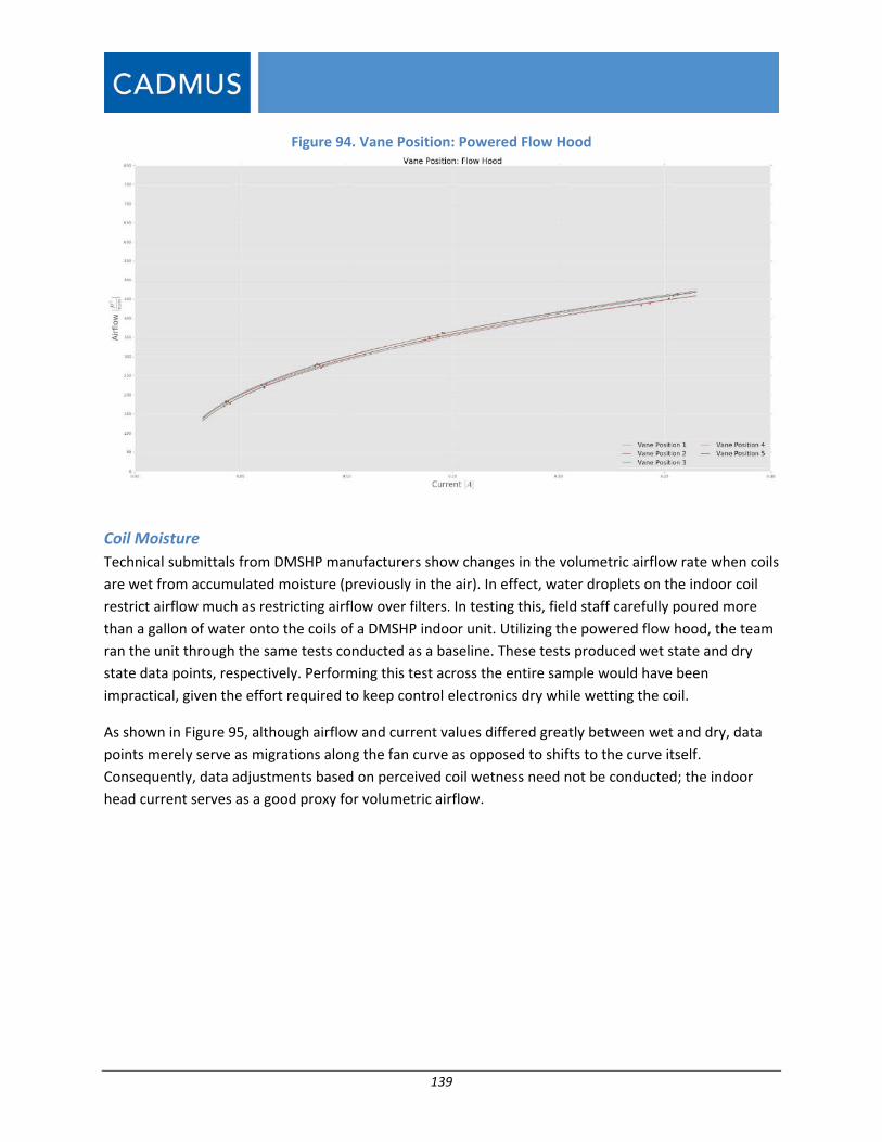
139

Figure 94. Vane Position: Powered Flow Hood

Coil Moisture

Technical submittals from DMSHP manufacturers show changes in the volumetric airflow rate when coils

are wet from accumulated moisture (previously in the air). In effect, water droplets on the indoor coil

restrict airflow much as restricting airflow over filters. In testing this, field staff carefully poured more

than a gallon of water onto the coils of a DMSHP indoor unit. Utilizing the powered flow hood, the team

ran the unit through the same tests conducted as a baseline. These tests produced wet state and dry

state data points, respectively. Performing this test across the entire sample would have been

impractical, given the effort required to keep control electronics dry while wetting the coil.

As shown in Figure 95, although airflow and current values differed greatly between wet and dry, data

points merely serve as migrations along the fan curve as opposed to shifts to the curve itself.

Consequently, data adjustments based on perceived coil wetness need not be conducted; the indoor

head current serves as a good proxy for volumetric airflow.

140

Figure 95. Coil State: Wet vs. Dry

Flow Restriction (Dirty Filter)

In using an indoor unit, a filter removes dust from the air, though this accumulates if not cleaned

regularly. As the filter accumulates dust and particles, the pressure drops across the filter increases, and

airflow is reduced. In a test setup, the evaluation team used foam inserts to simulate dirty filters.

Figure 96 shows the impact of restricting airflow to the DMSHP—the equivalent of a very dirty filter.

Similar to restrictions induced by wet and dry coils, restrictions induced by obstruction caused decreases

in the airflow quantity moved through the indoor unit. And, much like wet and dry coil results, when

accounting for the indoor fan current, changes were primarily migrations along the curve and not major

shifts of the fan curve itself. As seen in the figure, the vertical shift at a given fan amperage from the

averaged curve (dotted line) to the simulated dirty curve was less than 5%. Therefore, the team judged

that no data adjustments were needed to produce an airflow number within reasonable bounds, based

solely on current supplied to the fan.

141

Figure 96. Powered Flow Hood Flow Restriction

Resulting Experimental Design

Given the findings, the evaluation team chose to measure airflow using the methodology discussed in

earlier sections of this report.

142

Appendix B: Baseline Memorandum Chart

Logic Flow Chart to Determine Baseline, with Response Percentages (n = 116)

143

Appendix C: TRM Memorandum, December 2, 2016

To: Massachusetts and Rhode Island Program Administrators

From: COOL SMART Impact Evaluation Team

Subject: Ductless Mini‐Split Heat Pump Technical Reference Manual Recommendation

Date: December 2, 2016

This memo serves as a supplement to the forthcoming Ductless Mini‐Split Heat Pump Impact Evaluation

report prepared for the Massachusetts and Rhode Island Electric and Gas Program Administrators. It

discusses the methods and assumptions employed by the Massachusetts Technical Reference Manual

(TRM), from program years 2016‐2018, for calculating energy and demand savings resulting from

residential installations of ENERGY STAR® rated ductless mini‐split heat pumps (DMSHPs). Provided the

insights gained during the writing of the evaluation report, the basis of these TRM assumptions are

reviewed, and updated inputs and methods are recommended for future use.

Measure History The residential installation of an ENERGY STAR® rated DMSHP is categorized as a lost opportunity, HVAC

measure and specifically described as “The installation of a more efficient [DMSHP] system.” The

significance of being “more efficient” is in reference to the assumed baseline equipment of a minimally

efficient DMSHP, as determined by the Federal Register. Deemed energy and demand savings are

calculated from the following sets of equations:

Δ12 / 1 1 1 1

Δ12 / 1 1

Δ12 / 1 1

With quantities:

Δ = Reduction in annual kWh consumption of HP equipment

Δ = Summer reduction in electric demand of HP equipment

Δ = Winter reduction in electric demand of HP equipment

= Capacity of HP equipment

= Seasonal efficiency of baseline HP equipment

= Seasonal efficiency of new efficient HP equipment

= Peak efficiency of base HP equipment

144

= Peak efficiency of new efficient HP equipment

= Heating efficiency of baseline HP equipment

= Heating efficiency of new HP equipment

= EFLH for cooling

= EFLH for heating

Several assumptions are involved in these calculations, including 447 equivalent full load hours (EFLH)

for heating; 360 EFLH for cooling; and a baseline SEER, EER, and HSPF of 14, 10, and 8.2, respectively. A

TRM table provides various cases of high efficiency SEERs, EERs, and HSPFs and their resulting energy

and demand savings; these inputs and savings are replicated in for reference, drawing on past and

current TRM values.

Table 1. Savings for Residential DMSHPs

Year

2013, 2014 14.5 12.0 8.2 0.250 0.119 186

2013, 2014 19 12.83 10.0 0.331 0.448 669

2013, 2014 23 13 10.6 0.346 0.533 820

2015 14.5 12.0 8.2 0.515 0.000 13

2015 19 12.83 10.0 0.596 0.329 497

2015 23 13 10.6 0.611 0.414 648

2016 20.5 13.3 9.9 0.11 0.34 286

2016 24.2 13.8 12 0.11 0.45 330

Recommendations The assumed EFLH for cooling were greater than the same values calculated during the evaluation, as

shown in Table 2. The EFLH for heating were cited from a Cadmus memo providing initial results from

the DMSHP evaluation, and are in agreement with the final values reported in the study. The average of

the top 25% of EFLH are also included in .

Table 2. Heating and Cooling Equivalent Full Load Hours for DMSHP

Season MA TRM EFLH Measured EFLH Top 25% of Measured EFLH

Winter 2015 447 442 1,275

Summer 2015 360 218 499

Winter 2016 447 451 1,117

As part of the study, a second winter of on‐site metering was included, and so two sets of measured

heating EFLH values are presented above. One reason for this extension was the concern that the

unusually high amount of snowfall in 2015 would prevent the outdoor unit of the DMSHP from

operating at normal capacity, and result in lower EFLH. Although the measured EFLH from the two

145

winters are within three percent of each other, the evaluation team recommends using the 2016 value

as the data used in its calculation were collected under less extreme conditions. The assumed heating

EFLH vary slightly from the final values reported in the evaluation; these differences resulted from

refining the weather normalization method used by the evaluation team. The assumed cooling EFLH are

higher than the reported values, but the added context of where this assumption was drawn from is

important. The 360 EFLH for cooling were cited from an evaluation of central air conditioners, which the

evaluation team expects to operate more continuously than DMSHP systems. Given these findings, it is

recommended the TRM update the EFLH to 451 hours for heating and 218 hours for cooling.

The primary discrepancy between the current TRM methodology and that presented in this memo is the

determination of an appropriate baseline for calculating savings. The evaluation team found

homeowners frequently install DMSHP to displace existing HVAC systems or in lieu of some alternative;

because of this behavior, assuming all baseline systems are minimally efficient DMSHPs will fail to

accurately predict savings in many situations. Table 3 3 presents a concise set of baselines that were

observed during this study.

Table 3. Recommended DMSHP Baselines

Season Baseline Equipment Assumed Baseline Efficiency* Assumed Baseline Efficiency

for TRM Algorithm

Cooling

Ductless Heat Pump 14 SEER, 10 EER 14 SEER, 10 EER

Central Air Conditioner 13 SEER, 11 EER 13 SEER, 11 EER

Window Air Conditioner 9.8 EER 14.5 SEER**, 9.8 EER

Heating

Ductless Heat Pump 8.2 HSPF 8.2 HSPF

Boiler 0.82 AFUE 2.8 HSPF

Furnace 0.9 AFUE 2.6 HSPF***

Electric Resistance 1.0 COP 3.4 HSPF

*Massachusetts Technical Reference Manual for Estimating Savings from Energy Efficiency Measures. Tech. Massachusetts Electric and Gas Energy Efficiency Program Administrators, Oct. 2015. Web. Dec. 2016. < http://ma‐eeac.org/wordpress/wp‐content/uploads/2016‐2018‐Plan‐1.pdf >. **Because manufacturers do not report seasonal efficiencies for window air conditioning units, we have applied a scalar conversion factor derived from mean ratios between DHP EERs and SEERs values reported by AHRI. Acknowledging that window air conditioners generally do not have self‐regulating, variable speed motors like DHPs, which can contribute to lower seasonal efficiencies, we have averaged only DHP systems from the bottom half of the calculated ratios.

***Seasonal efficiency value includes an assumed 15% duck leakage, based on the MA PY 2016‐2018 TRM duct sealing measure.

There are many nuanced arguments surrounding exactly how a DMSHP baseline should be determined,

and for further discussion see the Baseline Memo, but for the purposes of a TRM algorithm the

evaluation team recommends a simple approach based on the equipment present in the home, and in

the absence of any coincident HVAC system, using a minimally efficient DMSHP baseline. By identifying a

site specific Assumed Baseline Seasonal Efficiency from Table 3, savings can be calculated from the sets

of equations currently presented in the TRM.

146

As a final recommendation, the evaluation team suggests that the actual SEER, EER, and HSPF ratings of

the newly installed DMSHP systems reported to and tracked by the PAs are used in the high efficiency

scenario of savings calculations. This change in the TRM methodology would acknowledge the wide

range of ratings available to consumers and the increasing seasonal efficiencies, and provide more

refined estimates of energy and demand reduction. Updating the residential, new installation DMSHP

TRM algorithm with the recommendations presented in this memo will result in a more current,

program specific, and data‐based methodology that is informed through extended study of this

measure.

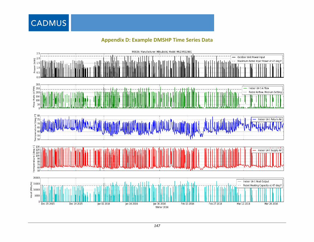
147

Appendix D: Example DMSHP Time Series Data

148

Documents

DMSHP Evaluation Report 12-30-2016 (without track changes)ma-eeac.org/wordpress/wp-content/uploads/Ductless-Mini-Split-Heat... · Unit Efficiency COP ... Table 14. Energy Savings,