Embed Size (px)
Citation preview

volume 7 pavement design and maintenance section 3 pavement maintenance assessment
part 2
Hd 29/08
data for pavement assessment
summarY
This Standard describes the data required for pavement assessment and the data collection methods that are currently approved by the Overseeing Organisations. These methods cover measurement of the construction and condition of different types of pavements, except skidding resistance which is covered in HD 28 (DMRB 7.3.1). This revision has been updated to reflect current practice and includes requirements previously issued in IAN 42/05.
instructions for use
1. Remove Contents pages from Volume 7 and insert new Contents pages for Volume 7 dated May 2008.
2. Remove HD 29/99 from Volume 7, Section 3 which is superseded by this Standard and archive as appropriate.
3. Insert HD 29/08 into Volume 7, Section 3.
4. Please archive this sheet as appropriate.
Note: A quarterly index with a full set of Volume Contents Pages is available separately from The Stationery Office Ltd.
design manual for roads and Bridges
may 2008

design manual for roads and Bridges Hd 29/08 volume 7, section 3, part 2
tHe HigHwaYs agencY
scottisH government
welsH assemBlY government llYwodraetH cYnulliad cYmru
tHe department for regional development nortHern ireland
Data for Pavement Assessment
Summary: This Standard describes the data required for pavement assessment and the data collection methods that are currently approved by the Overseeing Organisations. These methods cover measurement of the construction and condition of different types of pavements, except skidding resistance which is coveredinHD28(DMRB7.3.1).Thisrevisionhasbeenupdatedtoreflectcurrent practice and includes requirements previously issued in IAN 42/05.

may 2008
volume 7 section 3 part 2 Hd 29/08
registration of amendments
amend no
page no signature & date of incorporation of
amendments
amend no page no signature & date of incorporation of
amendments
registration of amendments

may 2008
volume 7 section 3 part 2 Hd 29/08
registration of amendments
amend no
page no signature & date of incorporation of
amendments
amend no page no signature & date of incorporation of
amendments
registration of amendments

volume 7 pavement design and maintenance section 3 pavement maintenance assessment
part 2
Hd 29/08
data for pavement assessment
contents
Chapter
1. Introduction
2. Traffic Speed Condition Surveys
3. Visual Condition Surveys
4. Deflectograph Testing
5. Falling Weight Deflectometer
6. Ground-Penetrating Radar (GPR)
7. Coring and Test Pits
8. References and Bibliography
9. Enquiries
Annexes
1. Not currently used
2. TRACS
A. Assessment Criteria B. Detailed Description of TRACS Condition Data
3. Not currently used
4. Deflectograph
A. Calibration B. Data Processing using PANDEF
5. Falling Weight Deflectometer (FWD)
A. Requirements for Consistency Checks B. FWD Surface Modulus and Reporting Template
6. Ground-Penetrating Radar (GPR)
A. Introduction to GPR B. Calibration of GPR for Determination of Layer Thickness C. Reporting the Results of a GPR Survey
design manual for roads and Bridges
may 2008

volume 7 section 3 part 2 Hd 29/08
chapter 1 introduction
1. introduction
mandatory sections
1.1 Sections of this document which form part of the Standards of the Overseeing Organisations are highlighted by being contained in boxes. These are the sections with which the Design Organisations must comply, or must have agreed a suitable alternative approach through a departure from Standard with the relevant Overseeing Organisation. The remainder of the document contains advice and enlargement which is commended to Design Organisations for their consideration.
scope
1.2 This Part describes the data required for pavement assessment and the data collection methods that are currently approved by the Overseeing Organisations. These methods cover measurement of the construction and condition of different types of pavements, except skidding resistance which is covered in HD 28 (DMRB 7.3.1). Guidance is also given on the processing of data obtained by the methods (where appropriate). Interpretation of the results is generally covered in HD 30 (DMRB 7.3.3) which also describes the use of each assessment method in the context of the overall pavement monitoring and assessment process. Advice on the interpretation of TRACS data (see Chapter 2) is given in this Part. The list of methods is not exhaustive and is not intended to exclude the use of other machines and methods. However, those which are presently part of the Overseeing Organisations’ standard assessment procedure are all included.
implementation
1.3 This Part must be used forthwith on all schemes for the improvement and maintenance of trunk roads including motorways currently being prepared, provided that, in the opinion of the Overseeing Organisation this would not result in significant additional expense or delay. Design organisations must confirm its application to particular schemes with the Overseeing Organisation.
u
m
H
may 2008
se in northern ireland
1.4 For use in Northern Ireland, this Standard will apply to those roads designated by the Overseeing Organisation.
utual recognition
1.5 The construction and maintenance of highway pavements will normally be carried out under contracts incorporating the Overseeing Organisations’ Specification for Highway Works (SHW) which is contained in the Manual of Contract Documents for Highway Works Volume 1 (MCHW 1). In such cases products conforming to equivalent standards and specification of other Member States (MS) of the European Economic Area (EEA) or a State which is party to a relevant agreement with the European Union and tests undertaken in other MS of the EEA or a State which is party to a relevant agreement with the European Union will be acceptable in accordance with the terms of Clauses 104 and 105 (MCHW 1.100). Any contract not containing these Clauses must contain suitable clauses of mutual recognition having the same effect, regarding which advice must be sought from the Overseeing Organisation.
ealth and safety
1.6 All surveys and data collection on or in the vicinity of highway pavements must be carried out in accordance with:
• Health and Safety at Work Act (1974);
• Management of Health and Safety at Work Regulations (1999);
• Construction (Design and Management) Regulations (2007) (CDM Regulations);
1/1

volume 7 section 3 part 2 Hd 29/08
chapter 1 introduction
• Traffic Signs Manual Chapter 8 (2006); and
• Safety at Street Works and Road Works – A Code of Practice.
1.7 In Northern Ireland, the relevant Health and Safety documents are:
• Construction (Design and Management) Regulations (Northern Ireland) 2007;
• Health and Safety at Work (Northern Ireland) Order 1978;
• Management of Health and Safety at Work Regulations (2000);
• Traffic Signs Manual Chapter 8 (2006); and
• Safety at Street Works and Road Works – A Code of Practice.
1.8 For the Highways Agency network, further information on Health and Safety is given in Part 1 of the Network Management Manual.
1.9 Where data collection involves excavating or driving probes into the subgrade at locations where there may be buried services, the public utility organisations must be contacted for details of the locations of their equipment. The exact location of buried services should be established prior to carrying out the work using cable locating equipment.
glossary
1.10 A glossary and list of principal abbeviations is given in HD 23 (DMRB 7.1.1).
1.11 The term “asphalt” replaces “bituminous material” as the generic term for pavement material consising of mineral aggregate combined with a bitumen binder and which is normally laid by a paver. “Asphalt” includes all bitumen bound base, binder course and surface course materials, except surface dressing. There are some exceptions to this as indicatedbelow, where “bituminous material” continues in use:
1/2
• Deflectograph processing uses the technical terms “Equivalent Thickness of Sound Bituminous Material (ESBM)”, “Total Thickness of Bituminous Material (TTBM)” and PANDEF Base Type Classification “BITS”. Use of the term “asphalt” would require changes to these acronyms and to text in the associated software.
• In some instances the term “bituminous materials” may also refer to surface dressings as well as paver laid material.
1.12 The term “Hydraulically Bound Mixture” or “HBM” is used as the generic term for pavement material consisting of mineral aggregate bound with cement, lime, slag or fly ash binder, or a combination thereof. The terms “lean concrete”, “cement bound material” or “CBM” are no longer used except in connection with PANDEF Base Type Classification “CEMT”.
may 2008

volume 7 section 3 part 2 Hd 29/08
ion surveYs
chapter 2 Traffic Speed Condition Surveys
2. traffic speed condit
types of surveys
2.1 On the trunk road network in England, surveys carried out under the Highways Agency (HA) TRAffic-speed Condition Survey (TRACS) contract replaced the previous High-speed Road Monitor (HRM) surveys in the summer of 2000. TRACS data is collected under a central HA contract which includes the loading of data to HAPMS for subsequent use by Agents and others.
2.2 On the National Network in Scotland, designated roads in Northern Ireland and on the Local Authority Road Network in England, traffic-speed surveys are carried out using the Surface Condition Assessment of the National NEtwork of Roads (SCANNER) system. On the National Network in Wales a method similar to SCANNER is used.
2fitot
Tt
2vaotmd
figure 2.1: tra
2.5 TRACS surveys are carried out annually usually over:
a) both lanes of single carriageways;
b) lanes 1 and 2 of the main carriageway on dual carriageways; and
c) lane 1 of slip roads.
Roundabouts are excluded from TRACS surveys. For precise details of the coverage and frequency of these surveys the HA should be consulted.
2sQi
2
•
•
may 2008
.3 The SCANNER survey details are given in the ve-volume User Guide and Specifications published by
he UK Roads Board (2007). A summary of the features f SCANNER surveys is given below, following the ext relating to TRACS surveys.
raffic-Speed Condition Survey (TRACS) (Relevant o the HA in England)
.4 TRACS surveys are carried out using survey ehicles equipped with lasers, video image collection nd inertia measurement apparatus to enable surveys f the road surface condition to be carried out whilst ravelling at variable speeds, of up to 100 km/h, to atch prevailing traffic, and hence cause minimum
isruption to other road users.
cs vehicle
.6 TRACS surveys are controlled by an end result pecification for the survey equipment and a detailed uality Audit procedure for the surveys includes regular
ndependent checks to maintain quality assurance.
.7 The TRACS survey vehicle measures:
Texture Profile in the nearside wheel-track at approximately 1mm longitudinal intervals;
Transverse Profile across a 3.2m width at approximately 0.15m longitudinal intervals;
2/1
volume 7 section 3 part 2 Hd 29/08
chapter 2 Traffic Speed Condition Surveys
• Longitudinal Profile in the nearside wheel-track at approximately 0.1m longitudinal intervals;
• cracking over a width of 3.2m (continuous monitoring);
• vehicle geographical position (Northing, Easting and altitude) as well as Road Geometry (gradient, crossfall and curvature) at discrete 5m intervals;
• a forward-facing video record of the road being surveyed;
• a downward-facing video record of the road being surveyed.
2.8 All data collected by the TRACS survey vehicle is referenced to the network sections to a longitudinal accuracy of ± 1m. The start and end points of sections are defined by Location Reference Points (LRPs) in Highways Agency Pavement Management System (HAPMS) referencing as described in the Network Management Manual (NMM).
2.9 The TRACS survey data is delivered in raw form as TRACS Raw Condition Data (RCD). The Highways Agency’s Machine Survey Pre-processor (MSP) software is used to process the RCD to generate the TRACS Base Condition Data (BCD), which contains:
• Rut Depths in the nearside and offside wheel-tracks calculated from the measured Transverse Profile, over 10m lengths;
• 3m, 10m and 30m Enhanced Longitudinal Profile Variance calculated from the measured Longitudinal Profile, averaged over 10m lengths for the nearside wheel-track only;
• Intensity of Cracking calculated from the crack map, over 10m lengths;
• Intensity of Wheel-track Cracking calculated from the crack map, over 10m lengths;
• Sensor Measured Texture Depth (SMTD), calculated from the measured Texture Profile, averaged over 10m lengths;
• crack map (refer to Annex 2B, clause 2B.17 for an explanation);
• an estimate of the level of Fretting present on the pavement, calculated from the measured Texture Profile, over 10m lengths;
2/2
• an estimate of the Surface Type, over 10m lengths;
• the road Geometry (gradient, crossfall and curvature), over 10m lengths;
• an estimate of the retroreflectivity of the road markings, over 100m lengths.
2.10 The TRACS BCD is loaded into HAPMS. HAPMS provides maintenance engineers with access to the condition data collected from their network, and enables them to identify potential maintenance schemes and to monitor network performance. The TRACS BCD can be queried in HAPMS and reported using the database facilities, and can be displayed against a map background. HAPMS also provides reports and information in support of the development of the Road Renewals maintenance programme. The on-line facilities in HAPMS provide a fuller guide to the presentation of project information.
2.11 TRACS survey data is reported within HAPMS in relation to the Sections defined for network referencing, but there may be gaps in the data. These gaps arise for a variety of reasons (e.g. where the survey vehicle drove out of lane due to obstructions or road works, or where the survey data has been identified as Unreliable).
2.12 From an examination of the TRACS condition data in HAPMS, lengths of road with deteriorating surface condition can be identified. Examples of the use of TRACS condition data include:
• Rut Depths can be used to evaluate safety and structural aspects of the pavement surface condition;
• the Longitudinal Profile Variance can be used to assess Ride Quality;
• Texture Depth data can be used to indicate a potential loss of skid resistance, in connection with SCRIM data, or provide warning of some modes of surface failure;
• the Cracking and Fretting data, together with the Surface Type data can be used to evaluate the condition of the surface.
assessment of road condition using tracs data
2.13 An overview of the condition, or the trend in condition, of road pavements is required to give an indication of the scale of possible maintenance
may 2008

volume 7 section 3 part 2 Hd 29/08
chapter 2 Traffic Speed Condition Surveys
requirements and to identify changes in the general level of service provided over a period of time. At a more detailed level, lengths of road requiring further investigation need to be identified and prioritised.
2.14 The results of an analysis of the TRACS survey data may be used as a coarse sift to identify lengths of road in need of further investigation or to supplement other road condition data to provide a robust road maintenance proposal. To undertake the assessment, the TRACS condition data (with the exception of TRACS Surface Type) must be obtained from HAPMS using the
category Definition
1 Sound – no visible deterioration.
2 Some deterioration – lower level of concer(project level) investigations are not needeparameters are at this category at isolated
3 Moderate deterioration – warning level of needs to be investigated. Priorities for morextent and values of the condition paramet
4 Severe deterioration – intervention level ofrequently on the motorway and all purposprevented this state from being reached. Ainvestigations should be carried out on theaction taken if, and as, appropriate.
table 2.1: condition categories for text
2.16 For any 100m length in Condition Category 4, a more detailed investigation should be carried out at the earliest opportunity and the need for maintenance assessed. Similarly, where two or more 100m lengths in Condition Category 3 fall within any 1km, the cause of the deterioration should be investigated to determine if maintenance or other actions are necessary. Priority for treatment will depend on the type, extent, distribution and severity of deterioration and the strategic objectives for road maintenance.
2.17 It is not appropriate to apply the classification system defined in Table 2.1 for the assessment of Cracking and Fretting. Annex 2A of this Part gives Guidance Levels which may be used in the interpretation of the values of these parameters reported in HAPMS.
2.18 When carrying out the assessment it is recommended that reference be made to the detailed descriptions and further guidance concerning the
may 2008
most recent TRACS Combined Length Weighted (LW) Averages data source. The TRACS Surface Type may be obtained using the HAPMS TRACS – Base Surface Type data source.
2.15 For Texture Depth, Rut Depth and Ride Quality, the TRACS survey data can be assessed by means of four Condition Categories, as shown in Table 2.1. These Condition Categories are defined by threshold values applicable to each parameter measured by the TRACS survey vehicle, which are set out in Annex 2A of this Part.
n. The deterioration is not serious and more detailed d unless extending over long lengths, or several positions.
concern. The deterioration is becoming serious and e detailed (scheme level) investigations depend on the ers.
f concern. This condition should not occur very e trunk road network as earlier maintenance must have t this level of deterioration more detailed (scheme level) deteriorated lengths at the earliest opportunity and
ure depth, rut depth and ride Quality
TRACS measurement of the Texture Profile, Transverse Profile, Longitudinal Profile, Cracking, Fretting and Noise given in Annex 2B of this Part. In particular, when determining the cause of significant levels of Cracking, it is recommended that the crack map be examined to determine the distribution and type of cracking present.
2.19 The Highways Agency must be contacted if more information is required about the interpretation of data collected under the TRACS contract.
assessment criteria for tracs data
general
2.20 This Section describes the interpretation of each of the condition parameters measured by the TRACS survey vehicle. The threshold levels or assessment criteria for evaluating the extent of pavement
2/3
volume 7 section 3 part 2 Hd 29/08
chapter 2 Traffic Speed Condition Surveys
deterioration are given in Annex 2A of this Part. The levels and criteria are based on experience gained from the HA’s ongoing research and development programme, and are currently considered to be the most appropriate criteria for condition assessment. However, they may change in the future as a result of further research.
2.21 All the threshold values and guidance levels are based on characteristic values associated with 100m lengths and are for the assessment of current TRACS data collected from in-service roads, as opposed to newly constructed roads.
tracs texture depth
2.22 Texture Depth values in the TRACS Combined Length Weighted (LW) Averages data source in HAPMS are calculated using the Sensor Measured Texture Depth (SMTD) method. The threshold values for TRACS (LW) Average Texture Depths are given in Table 2A.1 of Annex 2A of this Part.
2.23 Changes in the Texture Depth of the road surface can indicate a potential loss of skid resistance or some other mode of surface failure, e.g. Fretting (resulting in a high Texture Depth) (see also 2.37 to 2.39) or Fatting-up (resulting in a low Texture Depth). Advice on the interpretation of Texture Depth data in connection with skid resistance is given HD 28 (DMRB 7.3.1). HD 28 requires the Investigatory Level for skid resistance to be increased for surfaces (except High Friction Surfacing materials - HFS) with Texture Depth below 0.8mm SMTD (Category 3). Therefore, any location where the Texture Depth (except for HFS) triggers Category 3 or above must be reviewed in the context of HD 28.
2.24 Locations where the Texture Depth (except for HFS) triggers Category 4 will require urgent intervention if the nature of the surface condition means that further loss of texture can reasonably be expected, e.g. Fatting-up of a surface. Conversely, no action may be required if the Texture Depth is stable and a risk assessment undertaken in the context of HD28 does not indicate an elevated level of risk. Therefore, a more detailed investigation will be needed to determine the appropriate response.
2.25 Different thresholds are applied to High Friction Surfaces because of the different ways in which texture is provided by these materials. For these materials, the SMTD value is not an appropriate means of defining Condition Category 2 or higher. In this case, maintenance decisions must also take account of SCRIM results and the results of visual surveys.
t
2.th10rereinva
•
•
•
•
2.thRshthincoRchse
t
2.QLof(oloLpaAm
2.usvaw10wtoPTH
2/4
racs rut depth
26 HAPMS stores Rut Depth information as e average Rut Depth for each wheel-track over a m length. This base data is then used to calculate presentative values of rutting for the required porting lengths. HAPMS uses the stored rut formation to calculate the following LW Average lues:
Left Rut (using the left wheel-track values only);
Right Rut (using the right wheel-track values only);
Average Rut (using both wheel-track values);
Maximum Rut (using the maximum wheel-track values from each 10m).
27 Table 2A.2 of Annex 2A of this Part shows reshold values for the TRACS LW Average Maximum ut measurements. Note that concrete surfacings ould give negligible Rut Depths. It is recommended at, where any length has been identified for further vestigation as a result of high levels of rutting, mparison be made between the Left Rut and Right
ut LW Average values contained within HAPMS as a eck on the self-consistency of the rut measurements – e Annex 2B of this Part.
racs ride Quality
28 The measure used for the assessment of Ride uality, or Profile Unevenness, is the Enhanced ongitudinal Profile Variance of individual deviations the profile relative to a datum obtained by removing r filtering) longer wavelengths from the measured ngitudinal profile. This measure replaces the simpler ongitudinal Profile Variance and removes the effects of vement geometry (gradient, crossfall and curvature).
fuller description of the differences between the two easures is given in Annex 2B of this Part.
29 The assessment of Ride Quality is carried out ing three Enhanced Longitudinal Profile Variance lues, that indicate the level of profile unevenness ithin wavelength ranges less than or equal to 3m, m and 30m. It has been found that measurements
ithin these wavelength ranges may be broadly related levels of ride comfort. The Enhanced Longitudinal rofile Variance data is therefore reported within the RACS Length Weighted Averages data source in APMS as LPV 3m, LPV 10m and LPV 30m.
may 2008
volume 7 section 3 part 2 Hd 29/08
chapter 2 Traffic Speed Condition Surveys
2.30 The threshold values for the assessment of the TRACS LW Average Enhanced LPV measurements within the three wavelength ranges are given in Table 2A.2 of Annex 2A of this Part, and must be applied to all TRACS Enhanced LPV data reported in HAPMS. Note that different threshold values are specified within Table 2A.2 for different road classifications (which can be abstracted from HAPMS), e.g. a Motorway requires a better standard of Ride Quality than an urban single carriageway, where traffic is generally travelling at a lower speed.
tracs cracking
2.31 Guidance levels for the TRACS LW Average Whole Carriageway Cracking intensities are given in Table 2A.3 of Annex 2A of this Part. No guidance levels are currently specified for the intensity of Wheel-track Cracking
2.32 As described in Annex 2B of this Part, the TRACS survey vehicle relies on crack identification software to automatically identify cracks in the road surface. The measurement and the interpretation of the types of Cracking made by the crack identification software may differ from that made by an inspector carrying out a visual survey over the same site. As a result of this, the intensities of Cracking measured by the TRACS survey vehicle are generally lower than those recorded by a visual inspection. This behaviour is reflected by the low magnitudes for the guidance levels given in Table 2A.3 of Annex 2A of this Part.
2.33 Monitoring of the behaviour of the TRACS Cracking intensities recorded on the network has shown that they can be affected by variations in the survey conditions, which thereby influence the relative intensities of cracking reported. As a result, the intensities recorded in surveys carried out in consecutive survey years can vary and, when applying analyses based on threshold levels, the categories within which the Cracking measurements fall may change from survey year to survey year. Therefore:
• as the variability in the TRACS cracking intensities can introduce a degree of uncertainty in the cracking measurements, the thresholds defined in Table 2A.3 are provided for guidance only, to aid in identifying lengths in need of further investigation;
• it is not recommended that the intensities of cracking be used in the trending of pavement condition;
may 2008
• it is essential that, where any length has been identified for further investigation, examination be undertaken of the crack map data contained in HAPMS for the length under investigation before further action is taken;
• further advice regarding the assessment of the cracking data is provided in Annex 2B of this Part.
2.34 No thresholds are specified in Table 2A.3 of Annex 2A for the intensities of Whole Carriageway Cracking measured on concrete surfaces. Although the TRACS survey vehicle provides a measure of the extent of Cracking present on concrete surfaces it has been found that the system may falsely record the presence of joints or grooves in concrete roads as cracks. These false cracks are added to the Cracking area and lead to a higher level of Cracking being reported. Therefore, it is recommended that Cracking intensities derived from the TRACS crack data are not used to directly assess the condition of concrete surfaces within Condition Categories. However, for concrete surfaces the crack map may be utilised to aid in the assessment of the condition of the pavement.
tracs fretting
2.35 The Texture Profile data can be used for the estimation of the intensity of Fretting present on HRA surfaces. The guidance levels for the TRACS (LW) Average Fretting data are presented in Table 2A.4 of Annex 2A of this Part. However, the application of such data is relatively new and thresholds are provided for guidance only.
2.36 As the Fretting measure applies only to Hot Rolled Asphalt surfaces, the Surface Type must be known.
2.37 The Fretting measure can be used to assess the presence of minor deterioration and also aid in the assessment of Cracking. Guidance on the use of the Fretting measure is given in Annex 2B.
tracs predicted surface type
2.38 An estimate of the Surface Type can also be made from the TRACS Texture Profile data, within four categories:
• HRA;
• Thin Surfacing Systems;
2/5
volume 7 section 3 part 2 Hd 29/08
chapter 2 Traffic Speed Condition Surveys
• Brushed Concrete;
• Grooved Concrete.
2.39 The TRACS predicted Surface Type information may be obtained from the HAPMS TRACS – Base Surface Type Data data source in HAPMS.
2.40 The TRACS predicted Surface Type may be subject to error. The TRACS predicted Surface Type algorithms will always generate a predicted Surface Type, even when the true Surface Type does not fall within the four categories listed in paragraph 2.39. For example, the TRACS predicted Surface Type often reports High Friction Surfaces (which are not contained within the current list of identifiable surfaces) as brushed concrete.
2.41 The TRACS predicted Surface Type is probably of most use for defining where surface changes occur. Users may consider using HAPMS to plot the surface layer of the construction data alongside the TRACS predicted Surface Type to assist in the assessment of the accuracy of their construction records within HAPMS, which will remain the primary source of surface type information.
tracs road geometry
2.42 The TRACS survey vehicle records the instantaneous gradient, crossfall and radius of curvature of the pavement at intervals of 5m. The data values contained in the TRACS – Base Geometric Data are reported in units of percent (for gradient and crossfall) and metres (for radius of curvature). There are no thresholds specified for the assessment of geometric data.
TRACS Retroreflectivity
2.43 Retroreflectivity data is used to support the description of the condition of road markings. Its use is described in detail in DMRB Volume 8, Section 2, Part 2 (TD 26: Maintenance of road markings and road studs).
TRACS Video Records (Forward and Downward)
2.44 The TRACS survey vehicle is equipped with digital forward- and downward facing video cameras that collects a video record of the road being surveyed. The digital video image data is not accessible from within HAPMS but is transferred to hard disks (separate HA Areas being stored on separate disks), and the disks
2/6
distributed to each MA/MAC. The TRACS Forward Facing Video system, provided with the video images, is used to view the digitised video record.
2.45 The downward facing video records can be manually assessed to identify cracking and other surface defects which can be used as a preliminary stage to carrying out a full visual condition survey.
surface condition assessment of the national NEtwork of Roads (SCANNER)
2.46 This survey system has been developed by the UK Roads Board to provide a consistent method of measuring the surface condition of Local Authority road carriageways, using automated road condition survey machines, throughout the United Kingdom. Full details of the system are given in the User Guide and Specifications published by the UK Roads Board (2007). The following is only a brief overview of the system.
2.47 For information on any variations from the above Specification, applicable to Scotland or Wales, the relevant Overseeing Organisation should be consulted.
2.48 SCANNER consists of a Specification for the survey machines, a Specification for carrying out the surveys and a method of reporting road surface condition (the SCANNER Road Condition Indicator).
2.49 Before a survey vehicle can be used to carry out a SCANNER survey, it has to pass a very stringent set of accreditation tests each year. It must be operated with a defined Quality Assurance procedure and with an independent Auditor.
2.50 The survey data produced by the survey machines is loaded into a UKPMS-compliant pavement management system where it is processed to produce the SCANNER Road Condition Indicator (RCI) (England and Wales only) and for other highway maintenance and management purposes.
2.51 SCANNER was introduced to provide consistent, reliable survey data on the condition of road carriageways to support four separate requirements to:
• indicate the overall condition of a length of road carriageway, or of an area of a road network, to establish long term trends in road maintenance condition;
may 2008

volume 7 section 3 part 2 Hd 29/08
chapter 2 Traffic Speed Condition Surveys
• indicate the overall condition of a defined road network, as an outcome measure of local authority management and maintenance of their carriageway asset;
• produce indicative treatments and budget estimation, to plan carriageway maintenance at a network level;
• determine the optimum treatment timing, to prioritise treatment and minimise the whole life cost of maintenance at a scheme or project level.
2.52 SCANNER surveys are machine-based surveys that make a number of different measurements and process the measurements to provide a number of parameters that describe the condition of the road surface the:
• longitudinal profile along the road;
• transverse profile across the road;
• condition of the edge of the road;
• texture depth;
• presence and extent of surface cracking.
2.53 The SCANNER survey equipment makes many thousands of measurements within each 10m subsection along the carriageway. These are analysed and combined into a set of parameters which are reported as SCANNER parameter values for every 10m subsection along the road network. Even after the reduction of data to 10m SCANNER survey parameters, there is still too much data to be analysed by hand and the SCANNER data must be analysed through a pavement management system.
scanner road condition indicator
2.54 The SCANNER Road Condition Indicator (RCI) has been developed to characterise the overall condition of the road carriageway. The RCI is calculated from some of the parameters measured by SCANNER, in three stages:
• Each ‘measured parameter average value’ over a 10m subsection length is scored on a scale of 0 to 100 using an upper and lower threshold.
may 2008
• The scores of each separate parameter are combined using weightings to obtain a total number of points for each 10m subsection of the road. Each 10m subsection is then assigned to a condition “category” on the basis of the total points.
• The number of 10m subsections in each “category” are then totalled to give an overall figure for the section, the route or the network.
In the second stage, each 10m length is allocated to one of three condition categories – Red (poor overall condition – plan maintenance soon), Amber (some deterioration – needs investigation soon) and Green (in a good state of repair – no need to plan maintenance) – based on the total number of points. The overall condition assessment of a network is based on the proportions of the three condition categories of the total length of the network.
2.55 The thresholds, weightings and factors to be used in the RCI calculations are published on the UKPMS website and may vary over time.
2/7
volume 7 section 3 part 2 Hd 29/08
urveYs
chapter 3 visual condition surveys
3. visual condition s
Ha visual condition surveys
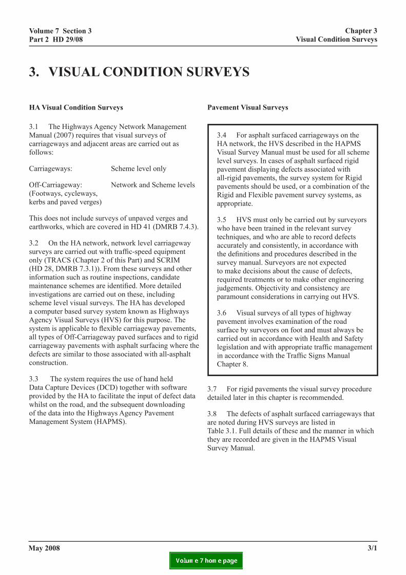
3.1 The Highways Agency Network Management Manual (2007) requires that visual surveys of carriageways and adjacent areas are carried out as follows:
Carriageways: Scheme level only
Off-Carriageway: Network and Scheme leve(Footways, cycleways, kerbs and paved verges)
This does not include surveys of unpaved verges and earthworks, which are covered in HD 41 (DMRB 7.4.
3.2 On the HA network, network level carriagewaysurveys are carried out with traffic-speed equipment only (TRACS (Chapter 2 of this Part) and SCRIM (HD 28, DMRB 7.3.1)). From these surveys and otherinformation such as routine inspections, candidate maintenance schemes are identified. More detailed investigations are carried out on these, including scheme level visual surveys. The HA has developed a computer based survey system known as Highways Agency Visual Surveys (HVS) for this purpose. The system is applicable to flexible carriageway pavementall types of Off-Carriageway paved surfaces and to rigcarriageway pavements with asphalt surfacing where defects are similar to those associated with all-asphaltconstruction.
3.3 The system requires the use of hand held Data Capture Devices (DCD) together with software provided by the HA to facilitate the input of defect dawhilst on the road, and the subsequent downloading of the data into the Highways Agency Pavement Management System (HAPMS).
may 2008
ls
3).
s, id
the
ta
pavement visual surveys
3.4 For asphalt surfaced carriageways on the HA network, the HVS described in the HAPMS Visual Survey Manual must be used for all scheme level surveys. In cases of asphalt surfaced rigid pavement displaying defects associated with all-rigid pavements, the survey system for Rigid pavements should be used, or a combination of the Rigid and Flexible pavement survey systems, as appropriate.
3.5 HVS must only be carried out by surveyors who have been trained in the relevant survey techniques, and who are able to record defects accurately and consistently, in accordance with the definitions and procedures described in the survey manual. Surveyors are not expected to make decisions about the cause of defects, required treatments or to make other engineering judgements. Objectivity and consistency are paramount considerations in carrying out HVS.
3.6 Visual surveys of all types of highway pavement involves examination of the road surface by surveyors on foot and must always be carried out in accordance with Health and Safety legislation and with appropriate traffic management in accordance with the Traffic Signs Manual Chapter 8.
3.7 For rigid pavements the visual survey procedure detailed later in this chapter is recommended.
3.8 The defects of asphalt surfaced carriageways that are noted during HVS surveys are listed in Table 3.1. Full details of these and the manner in which they are recorded are given in the HAPMS Visual Survey Manual.
3/1

volume 7 section 3 part 2 Hd 29/08
chapter 3 visual condition surveys
defect Definition
1 Major Area Cracking Single or multipleas Transverse Crac
2 Minor Area Cracking Single or multipleclassified as Trans
3 Major Crazing Interlocking patter
4 Minor Crazing Interlocking patter
5 Major Fatting Bitumen in the sur
6 Minor Fatting Bitumen in the suraggregate.
7 Mud Pumping The visible presenpavement. The occof at least 1 square
8 Patching Failure Patches or reinstatover any part of thcracking.
9 Major Surface Defectiveness
Loss of material frsurface is not discechippings.
10 Minor Surface Defectiveness
Loss of material frsurface is still disc
11 Major Transverse Crack Single or multipleangles to the centr
12 Minor Transverse Crack Single or multipleangles to the centr
Table 3.1: HVS C
Off-Carriageway Visual Surveys
3.9 Visual Surveys of Off-Carriageway items (footways, cycleways and paved verges) are used at network level to:
• assist in the identification of areas requiring planned maintenance, and to provide information to enable potential maintenance schemes on Off-Carriageway features to be assessed and prioritised;
• allow the overall conditions of the Trunk Road Off- Carriageway network to be monitored for reporting purposes.
3/2
non-interlocking cracks (>1mm wide) and not classified king.
non-interlocking cracks (<=1mm wide) and not verse Cracking.
n of cracks (>1mm wide).
n of cracks (<=1mm wide).
face course is flush or covering the coarse aggregate.
face course is close to but below the top of the coarse
ce of fines emanating from a crack/hole/joint in the urrence is accompanied by a cracked or depressed area metre in asphalt pavements.
ements that have subsided or rutted more than 10mm e patch/reinstatement or that exhibit more than 20%
om the wearing surface to a degree that the original rnible. Includes Chipping Loss from Surface applied
om the wearing surface to a degree that the original ernible.
cracks (> 0.1m spaced) cracks, >1mm wide, at right e line.
cracks (> 0.1m spaced) cracks, ≤ 1mm wide, at right e line.
arriageway Defects
3.10 All Off-Carriageway network or scheme level visual surveys on the HA network must be carried out using the HVS described in the HAPMS Visual Survey Manual.
3.11 The Off-Carriageway elements in HVS may be constructed from asphalt, concrete or block paving. Non-paved surfaces are not included. The defects to be recorded depend to some degree on the type of surfacing and include:
• major and minor cracking;
• major and minor local settlement or subsidence;
• major and minor fretting;
• longitudinal trip;
may 2008
volume 7 section 3 part 2 Hd 29/08
chapter 3 visual condition surveys
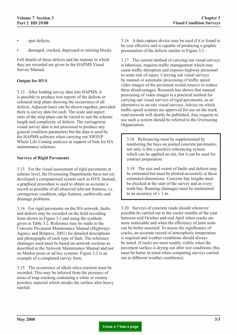
• spot defects;
• damaged, cracked, depressed or missing blocks.
Full details of these defects and the manner in which they are recorded are given in the HAPMS Visual Survey Manual.
output for Hvs
3.12 After loading survey data into HAPMS, it is possible to produce text reports of the defects or coloured strip plans showing the occurrence of all defects. Adjacent lanes can be shown together, provided there is survey data for each. The scale and aspect ratio of the strip plans can be varied to suit the scheme length and complexity of defects. The carriageway visual survey data is not processed to produce any general condition parameters but the data is used by the HAPMS software when carrying out SWEEP Whole Life Costing analyses in support of bids for HA maintenance schemes.
surveys of rigid pavements
3.13 For the visual assessment of rigid pavements at scheme level, the Overseeing Departments have not yet developed a computerised system such as HVS. Instead, a graphical procedure is used to obtain as accurate a record as possible of all observed relevant features, i.e. carriageway condition, edge features, earthworks and drainage problems.
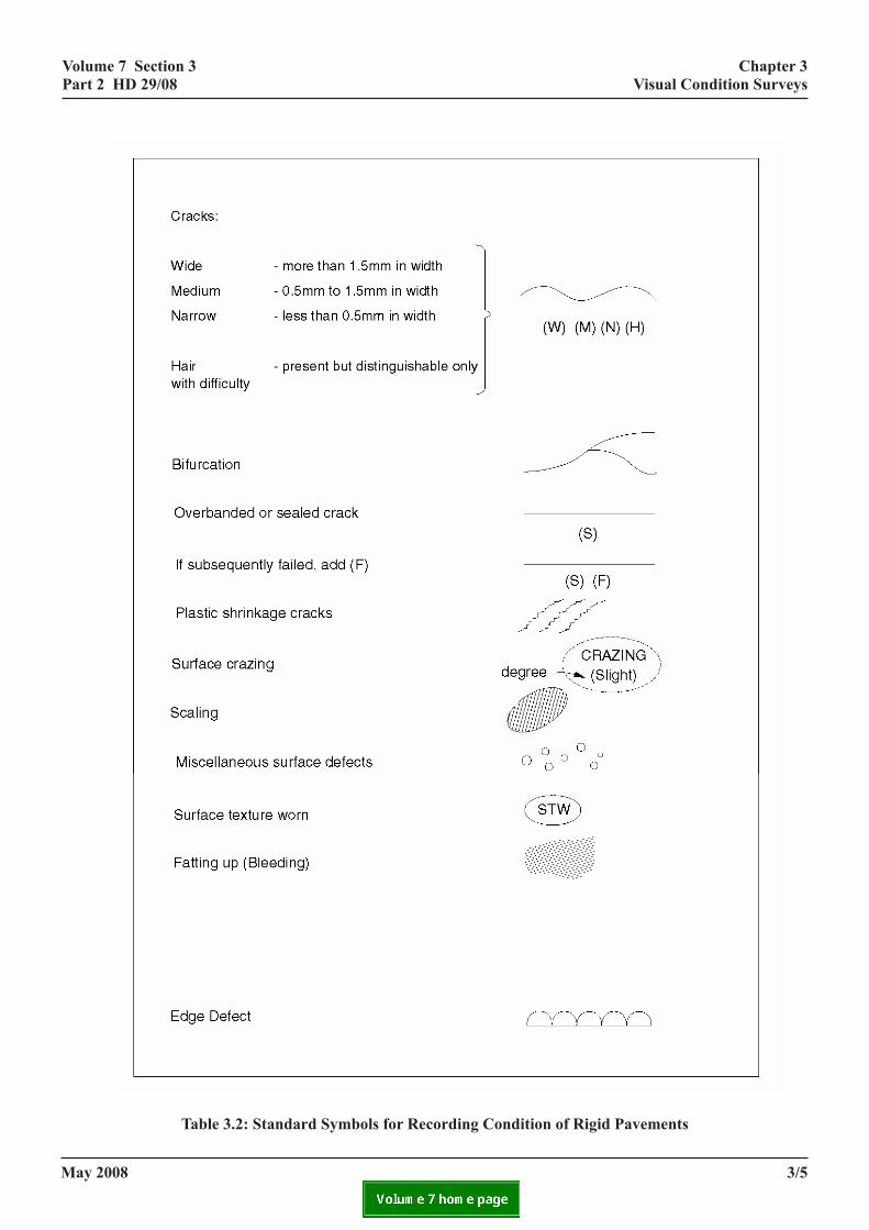
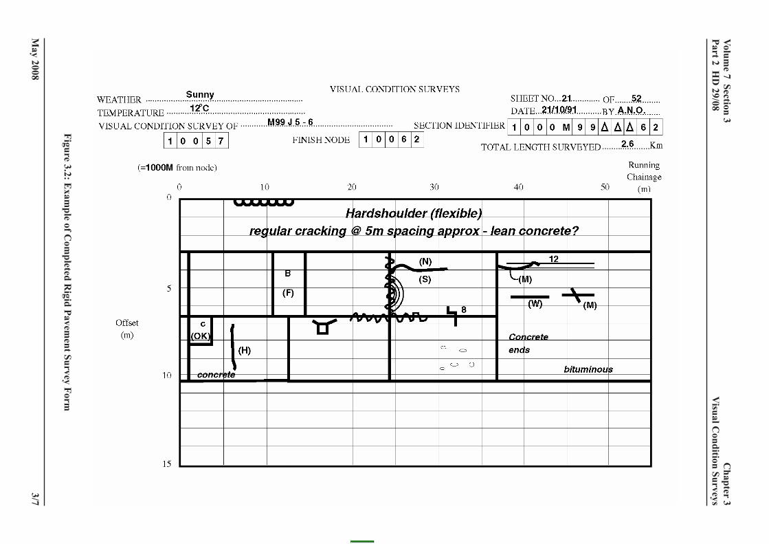
3.14 For rigid pavements on the HA network, faults and defects may be recorded on the field recording form shown in Figure 3.1 and using the symbols given in Table 3.2. Reference may be made to the Concrete Pavement Maintenance Manual (Highways Agency and Britpave, 2001) for detailed descriptions and photographs of each type of fault. The reference chainages used must be based on network sections as described in the Network Maintenance Manual and not on Marker posts or ad hoc systems. Figure 3.2 is an example of a completed survey form.
3.15 The occurrence of alkali-silica reaction must be recorded. This may be inferred from the presence of areas of map cracking containing a white or creamy powdery material which streaks the surface after heavy rainfall.
3bp
3ictbvtpcatruO
3pbmccibpmo
may 2008
.16 A data capture device may be used if it is found to e cost effective and is capable of producing a graphic resentation of the defects similar to Figure 3.1.
.17 The current method of carrying out visual surveys s laborious, requires traffic management which may ause traffic disruption and exposes highway personnel o some risk of injury. Carrying out visual surveys y manual or automatic processing of traffic speed ideo images of the pavement would remove or reduce hese disadvantages. Research has shown that manual rocessing of video images is a practical method for arrying out visual surveys of rigid pavements, as an lternative to on-site visual surveys. Advice on which raffic-speed systems are approved for use on the trunk oad network will shortly be published. Any requests to se such a system should be referred to the Overseeing rganisation.
3.18 Referencing must be supplemented by numbering the bays on jointed concrete pavements; not only is this a positive referencing system which can be applied on site, but it can be used for contract preparation.
3.19 The size and extent of faults and defects may be estimated but must be plotted accurately at these estimated dimensions. Concrete bay lengths must be checked at the start of the survey and at every tenth bay. Running chainages must be maintained to an accuracy of ± 1 m.
.20 Surveys of concrete roads should whenever ossible be carried out in the cooler months of the year etween mid October and mid April when cracks are ore noticeable and when the efficiency of joint seals
an be better assessed. To assess the significance of racks, an accurate record of atmospheric temperature s required and weather conditions should always e noted. (Cracks are most readily visible when the avement surface is drying out after wet conditions; this ust be borne in mind when comparing surveys carried
ut in different weather conditions).
3/3

may 2008
volume 7 section 3
part 2 Hd
29/08
3/4
chapter 3
visual c
ondition surveysC
hapter 3 V
olume 7 Section 3
V
isual Condition Surveys
Part 2 HD
29/08
3/4 January 2008
figure 3.1: rigid pavem
ent survey form
Figure 3.1 Rigid Pavem
ent Survey Form
m
volume 7 section 3 part 2 Hd 29/08
chapter 3 visual condition surveysVolume 7 Section 3 Chapter 3
Part 2 HD 29/08 Visual Condition Surveys
table 3.2: standard symbols for recording condition of rigid pavements
Table 3.2 Standard Symbols for Recording Condition of Rigid Pavements
ay 2008 3/5January 2008 3/5

volume 7 section 3 part 2 Hd 29/08
3/6
chapter 3 visual condition surveysChapter 3 Volume 7 Section 3
Visual Condition Surveys Part 2 HD 29/08
3
Table 3.2 (continued): Standard Symbols for Recording Condition of Rigid Pavements
TABLE 3.2 (continued) Standard Symbols for Recording Condition of Rigid Pavements
Asphalt - B Cementitious - C Epoxy - E Add (OK) if sound or (F) if failed
may 2008/6 January 2008
may 2008
volume 7 section 3
part 2 Hd
29/08
3/7
chapter 3
visual c
ondition surveys
Volum
e 7 Section 3 C
hapter 3 Part 2 H
D 29/08
Visual C
ondition Surveys January 2008
3/7
figure 3.2: exam
ple of com
pleted rigid pavem
ent survey form
Figure 3.2 Exam
ple of Com
pleted Rigid Pavem
ent Survey Form

volume 7 section 3 part 2 Hd 29/08
chapter 3 visual condition surveys
continuously reinforced concrete pavements (CRCP)
3.21 Experience with visual assessment of continuously reinforced concrete pavements to date is limited. The Overseeing Organisations can therefore only give general guidance on visual survey methods.
3.22 CRCP construction has no transverse movement joints to accommodate longitudinal movement, and as a consequence transverse shrinkage cracks spaced between 1m and 4m develop shortly after construction over the total area of the slab. As time passes additional transverse cracks slowly develop between the wider spaced cracks. All these cracks are held closed by a continuous layer of heavy reinforcement, thus maintaining aggregate interlock and ensuring transfer of load across the cracks. Such cracking is considered normal for this type of construction and its presence does not indicate significant failure or weakness.
3.23 These “normal” cracks are defined as follows:
• the cracks are exclusively transverse with no spalling or bifurcations;
• less than 1mm width;
• spaced at least 1m apart.
3.24 Significant defects, indicating a weakened structure or need for maintenance, include:
• transverse cracks at spacings of less than 1m;
• transverse cracks with widths greater than 1mm;
• longitudinal cracks;
• areas of polygonal cracking;
• loose or missing blocks of concrete;
• crack bifurcations;
• failing repairs;
• spalling.
3/8
3.25 Similar visual survey methods to those used for jointed pavements should be used for surveying CRCP except that:
• the “normal” cracking is only recorded for the first 10m in every 100m length;
• the significant defects defined in 3.24 are recorded for the entire length;
• at CRCP terminations (involving ground beams), all “normal” cracking, significant defects and slab features must be recorded for the adjacent 100m of the pavement.
3.26 Guidance on the interpretation of visual survey data is given in HD 30 (DMRB 7.3.3).
presentation
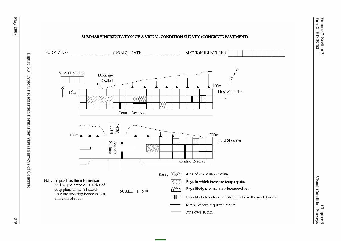
3.27 Field survey sheets, or a fair copy, must be retained. The general condition of the road must be summarised on a plan to a suggested scale of 1:500. A typical form of presentation is shown in Figure 3.3. A record at this scale must also include notes about particular areas where the condition or rate of deterioration needs to be monitored during subsequent inspections.
3.28 The distribution and incidence of faults and defects is likely to be an important pointer to future performance. It may be useful to show the percentage distribution of defects in the following three categories:
a) defects likely to lead to safety hazards or serious surface deterioration within the next year;
b) defects which immediately affect user comfort or convenience, e.g. faulting or settlement;
c) defects likely to affect structural integrity within the next 3 year period.
3.29 This distribution should be compared with those given in earlier surveys. Summaries must also make clear whether existing repairs fall into the category of temporary or permanent. The material used for the repair must be recorded.
may 2008
may 2008
volume 7 section 3
part 2 Hd
29/08
3/9
chapter 3
visual c
ondition surveysC
hapter 3 V
olume 7 Section 3
V
isual Condition Surveys
Part 2 HD
29/08
3/10 January 2008
figure 3.3: typical presentation format for v
isual surveys of concrete
Figure 3.3 Typical Presentation Form
at for Visual Surveys of C
oncrete
Asphalt
Surface

volume 7 section 3 part 2 Hd 29/08
ing
chapter 4 Deflectograph Testing
4. deflectograpH test
general
4.1 This chapter describes the Deflectograph and the processing of its output. The Deflectograph is used to assess the structural condition of flexible pavements. It works on the principle that as a loaded wheel passes over the pavement, the pavement deflects and the size of the deflection is related to the strength of the pavement layers and subgrade.
4.2 The survey speed is slow (2.5 km/h) and consequently Deflectograph surveys cause considerable disruption, particularly on heavily trafficked roads. On the HA network this type of survey is no longer carried out at network level and is only used in support of individual maintenance schemes. However, other Overseeing Organisations may continue to use the Deflectograph at a network level. Ongoing research of a Traffic Speed Deflectometer (TSD) offers the potential to obtain Deflectograph type data from a survey vehicle traveling at speeds up to 80 km/h.
4.3 The assessment procedure used depends on the type of pavement and its mode of deterioration. Some thick, well constructed flexible pavements with asphalt base have been found not to deteriorate in the conventional way and with timely attention to surface defects can have a long but indeterminate life.
TwctD
d
4dldiIsp
4Dmfstttpf
may 2008
Figure 4.1
hese potentially long-life pavements are identified ith deflection and thickness criteria. The structural
ondition of other flexible pavements is assessed in erms of residual life using a long-established Deflection esign Method based on deflection and traffic loading.
eflectograpH
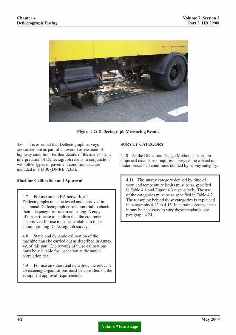
.4 The Deflectograph (Figure 4.1) is an automated eflection measuring system. It is a fully self-contained orry-mounted system, whereby measurements of eflection are taken at approximately 4m intervals n both wheel-tracks while the machine is in motion. t is regarded by the Overseeing Organisation as the tandard deflection measuring device for use on flexible avements.
.5 The transient deflection is measured as the eflectograph travels slowly along the line of twin easurement beams which are attached to a reference
rame. The measurement is not an absolute value of urface deflection since the reference frame sits within he wheelbase of the lorry and is itself influenced by he load. It represents a repeatable measure but since he analysis method is empirical, it is important that the rocedures for the use of the Deflectograph are closely ollowed.
4/1
: Deflectograph
volume 7 section 3 part 2 Hd 29/08
chapter 4 Deflectograph Testing
Figure 4.2: Deflectograph
4.6 It is essential that Deflectograph surveys are carried out as part of an overall assessment of highway condition. Further details of the analysis and interpretation of Deflectograph results in conjunction with other types of pavement condition data are included in HD 30 (DMRB 7.3.3).
machine calibration and approval
4.7 For use on the HA network, all Deflectographs must be tested and approved in an annual Deflectograph correlation trial to check their adequacy for trunk road testing. A copy of the certificate to confirm that the equipment is approved for use must be available to those commissioning Deflectograph surveys.
4.8 Static and dynamic calibration of the machine must be carried out as described in Annex 4A of this part. The records of these calibrations must be available for inspection at the annual correlation trial.
4.9 For use on other road networks, the relevant Overseeing Organisations must be consulted on the equipment approval requirements.
su
4.emun
4/2
Measuring Beams
rveY categorY
10 As the Deflection Design Method is based on pirical data its use requires surveys to be carried out der prescribed conditions defined by survey category.
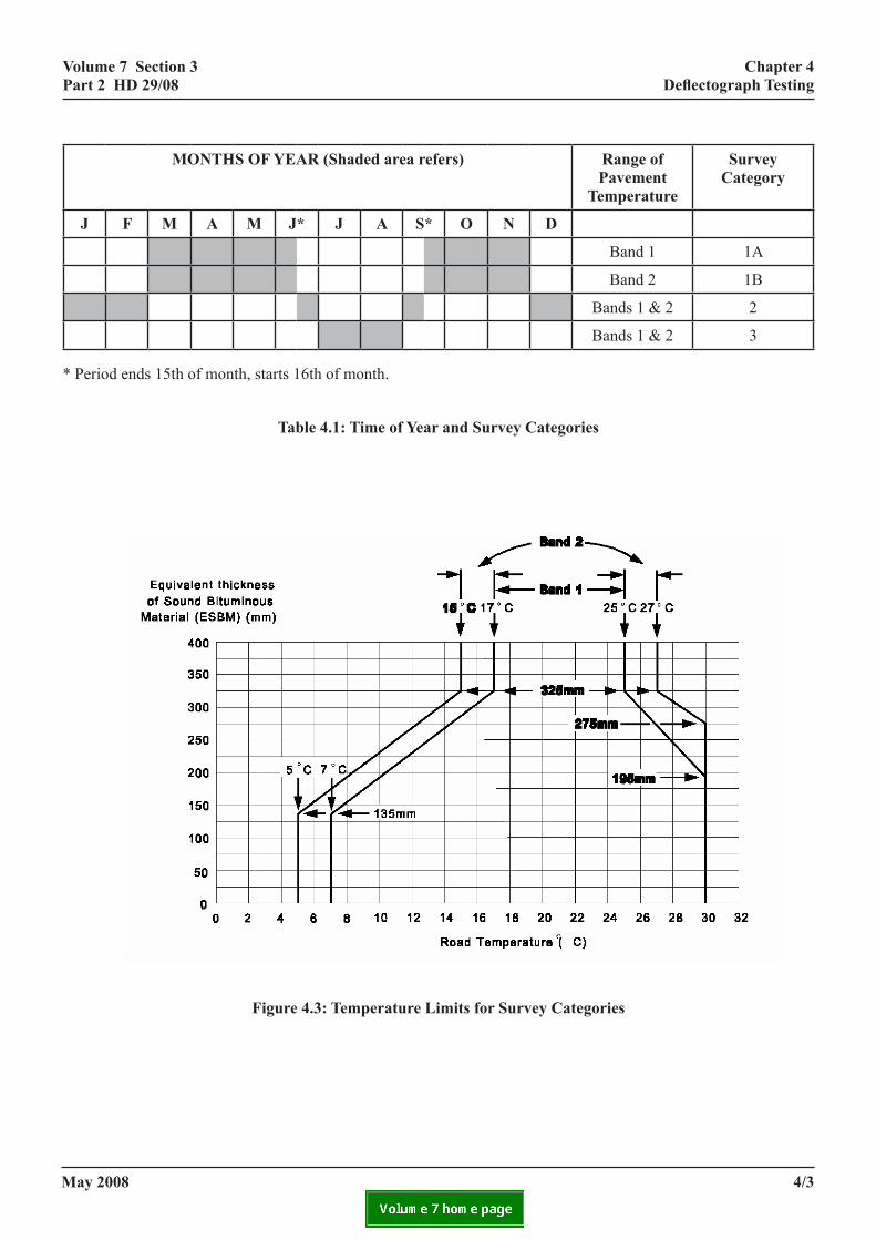
4.11 The survey category defined by time of year, and temperature limits must be as specified in Table 4.1 and Figure 4.3 respectively. The use of the categories must be as specified in Table 4.2. The reasoning behind these categories is explained in paragraphs 4.12 to 4.15. In certain circumstances it may be necessary to vary these standards, see paragraph 4.24.
may 2008
volume 7 section 3 part 2 Hd 29/08
chapter 4 Deflectograph Testing
Volume 7 Section 3 Chapter 4 Part 2 HD 29/08 Deflectograph Testing
MONTHS OF YEAR (Shaded area refers) range of pavement
temperature
survey category
J f m a m J* J a s* o n d
Band 1 1A
Band 2 1B
Bands 1 & 2 2
Bands 1 & 2 3
* Period ends 15th of month, starts 16th of month.
table 4.1: time of Year and survey categories
figure 4.3: temperature limits for survey categories
MONTHS OF YEAR (Shaded area refers) Range of Pavement
Temperature
Survey Category
J F M A M J* J A S* O N D
Band 1 1A
Band 2 1B
Bands 1 & 2 2
Bands 1 & 2 3
* Period ends 15th of month, starts 16th of month.
Table 4.1 Time of Year and Survey Categories
Figure 4.3 Temperature Limits for Survey Categories
may 2008 4/3
January 2008 4/3
volume 7 section 3 part 2 Hd 29/08
minimum category required
e a change in use is
1A with not greater than
10% in 1B
(at least one further survey 2
chapter 4 Deflectograph Testing
purpose of survey
To finalise the details of a Maintenance Scheme
To identify cause of surface damage already evident or wherproposed which will result in increased traffic loading
To provide advanced information for maintenance planning expected before strengthening measures defined)
Relative assessment within a site
Table 4.2: Survey Specificat
4.12 CATEGORY 1A defines the preferred conditions for deflection surveys. The highest confidence may be placed on the results of surveys in this category. The identification of potentially long-life pavements must be based on a Category 1A survey.
4.13 CATEGORY 1B extends the upper and lower limits of the temperature range allowed by including Band 2. This category is intended to allow for the situation that may arise when a survey planned for Category 1A does not comply with the specification because of unexpected changes in temperature taking place during the course of a survey.
4.14 CATEGORY 2. The wider temperature range obtained by adding Band 1 to Band 2 also applies to this category. The first part of September is included in Category 2 because after a hot dry summer, drying out of the subgrade may lead to measured deflections which do not truly reflect the weakest condition of the pavement.
4.15 CATEGORY 3. Surveys must not normally be carried out during the summer months specified for this category because of the difficulty of obtaining reliable, reproducible results.
equivalent thickness of sound Bituminous material (ESBM)
4.16 Deflection of asphalt pavements varies with temperature. The susceptibility to change in temperature is dependent on the thickness, age and condition of the asphalt layers. The parameter ESBM attempts to embody these factors and is only calculated for the purposes of correction of deflection to a standard temperature. It does not in any way reflect the structural contribution of the asphalt (bituminous) layers.
4.toaucobesoorwpothstr
ea
4/4
3
ion for Trunk Roads
17 ESBM is required for correction of deflection the standard temperature of 20oC and is calculated tomatically during processing following input of nstruction information. The asphalt type needs to defined as dense or non-dense and its condition as und or unsound. Materials such as hot rolled asphalt dense bituminous macadam are defined as dense hilst materials such as open textured macadam or rous asphalt are non-dense. Unsound materials are ose showing cracking, disintegration or evidence of ipping.
4.18 Asphalt pavement layers comprising multiple surface dressings (where the total thickness is less than 25mm), any asphalt layers beneath hydraulically-bound layers and any asphalt layers with their upper surface at greater than a 200mm depth and separated from the higher asphalt layers by granular layer, must be ignored.
rly life surveys
4.19 Surveys carried out within two years of a new road being opened or a road having had a major strengthening treatment must not be used to determine residual life or strengthening requirements. This is because the early life deflections can be more variable and are not a reliable indicator of future structural strength of a pavement until the pavement and subgrade have stabilised, which usually takes at least two years.
may 2008
volume 7 section 3 part 2 Hd 29/08
chapter 4 Deflectograph Testing
permitted temperature range
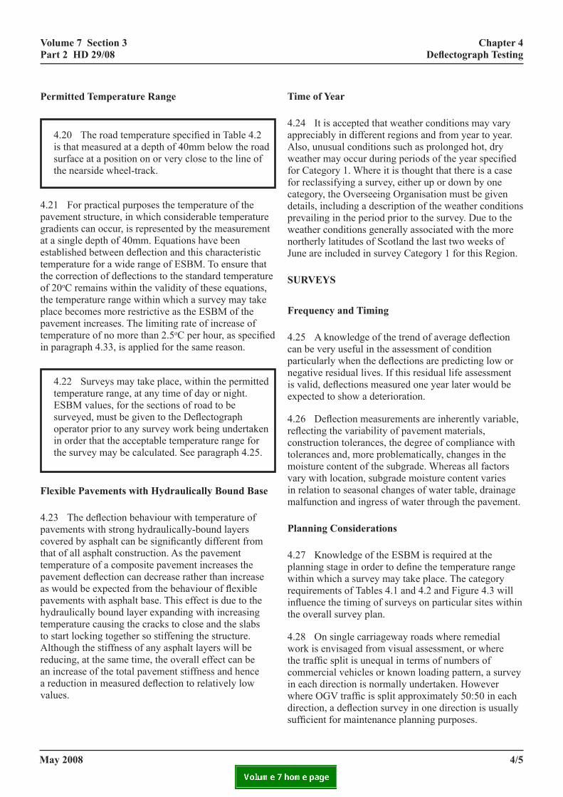
4.20 The road temperature specified in Table 4.2 is that measured at a depth of 40mm below the road surface at a position on or very close to the line of the nearside wheel-track.
4.21 For practical purposes the temperature of the pavement structure, in which considerable temperature gradients can occur, is represented by the measurement at a single depth of 40mm. Equations have been established between deflection and this characteristic temperature for a wide range of ESBM. To ensure that the correction of deflections to the standard temperature of 20oC remains within the validity of these equations, the temperature range within which a survey may take place becomes more restrictive as the ESBM of the pavement increases. The limiting rate of increase of temperature of no more than 2.5oC per hour, as specified in paragraph 4.33, is applied for the same reason.
4.22 Surveys may take place, within the permitted temperature range, at any time of day or night. ESBM values, for the sections of road to be surveyed, must be given to the Deflectograph operator prior to any survey work being undertaken in order that the acceptable temperature range for the survey may be calculated. See paragraph 4.25.
Flexible Pavements with Hydraulically Bound Base
4.23 The deflection behaviour with temperature of pavements with strong hydraulically-bound layers covered by asphalt can be significantly different from that of all asphalt construction. As the pavement temperature of a composite pavement increases the pavement deflection can decrease rather than increase as would be expected from the behaviour of flexible pavements with asphalt base. This effect is due to the hydraulically bound layer expanding with increasing temperature causing the cracks to close and the slabs to start locking together so stiffening the structure. Although the stiffness of any asphalt layers will be reducing, at the same time, the overall effect can be an increase of the total pavement stiffness and hence a reduction in measured deflection to relatively low values.
t
4.apAwfofocadeprwnoJu
s
f
4.capaneisex
4.recotomvainm
p
4.plwreinth
4.wthcoinwdi
may 2008
ime of Year
24 It is accepted that weather conditions may vary preciably in different regions and from year to year. lso, unusual conditions such as prolonged hot, dry eather may occur during periods of the year specified r Category 1. Where it is thought that there is a case r reclassifying a survey, either up or down by one tegory, the Overseeing Organisation must be given tails, including a description of the weather conditions evailing in the period prior to the survey. Due to the eather conditions generally associated with the more rtherly latitudes of Scotland the last two weeks of ne are included in survey Category 1 for this Region.
urveYs
requency and timing
25 A knowledge of the trend of average deflection n be very useful in the assessment of condition rticularly when the deflections are predicting low or gative residual lives. If this residual life assessment
valid, deflections measured one year later would be pected to show a deterioration.
26 Deflection measurements are inherently variable, flecting the variability of pavement materials, nstruction tolerances, the degree of compliance with lerances and, more problematically, changes in the oisture content of the subgrade. Whereas all factors ry with location, subgrade moisture content varies relation to seasonal changes of water table, drainage alfunction and ingress of water through the pavement.
lanning considerations
27 Knowledge of the ESBM is required at the anning stage in order to define the temperature range ithin which a survey may take place. The category quirements of Tables 4.1 and 4.2 and Figure 4.3 will fluence the timing of surveys on particular sites within e overall survey plan.
28 On single carriageway roads where remedial ork is envisaged from visual assessment, or where e traffic split is unequal in terms of numbers of mmercial vehicles or known loading pattern, a survey each direction is normally undertaken. However here OGV traffic is split approximately 50:50 in each rection, a deflection survey in one direction is usually
sufficient for maintenance planning purposes.
4/5
volume 7 section 3 part 2 Hd 29/08
chapter 4 Deflectograph Testing
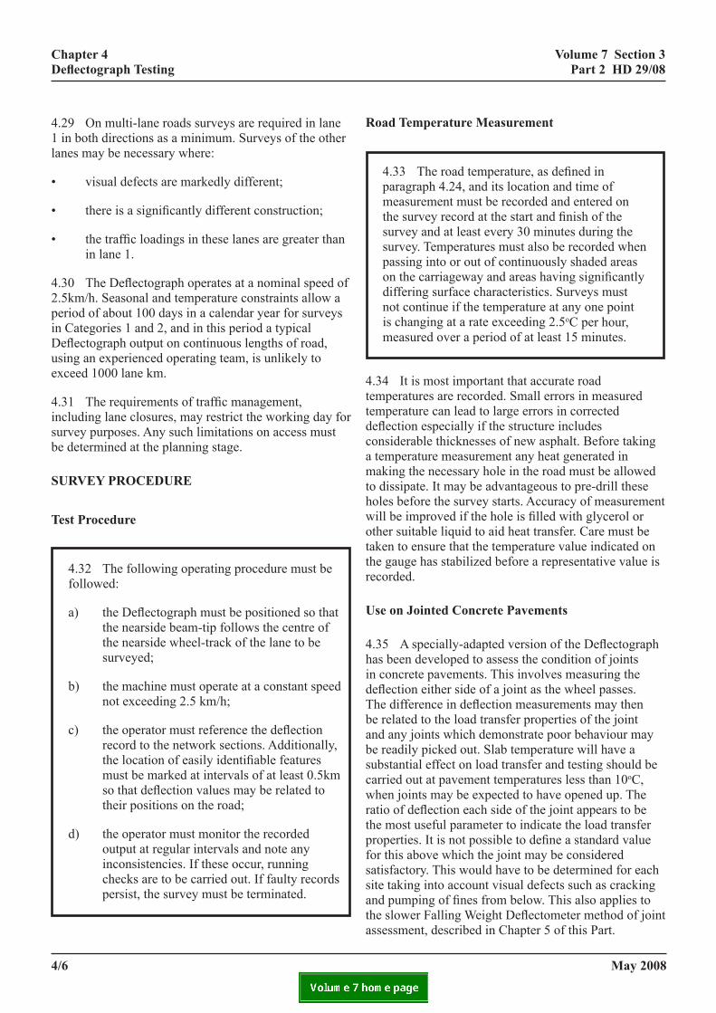
4.29 On multi-lane roads surveys are required in lane 1 in both directions as a minimum. Surveys of the other lanes may be necessary where:
• visual defects are markedly different;
• there is a significantly different construction;
• the traffic loadings in these lanes are greater than in lane 1.
4.30 The Deflectograph operates at a nominal speed of 2.5km/h. Seasonal and temperature constraints allow a period of about 100 days in a calendar year for surveys in Categories 1 and 2, and in this period a typical Deflectograph output on continuous lengths of road, using an experienced operating team, is unlikely to exceed 1000 lane km.
4.31 The requirements of traffic management, including lane closures, may restrict the working day for survey purposes. Any such limitations on access must be determined at the planning stage.
surveY procedure
test procedure
4.32 The following operating procedure must be followed:
a) the Deflectograph must be positioned so that the nearside beam-tip follows the centre of the nearside wheel-track of the lane to be surveyed;
b) the machine must operate at a constant speed not exceeding 2.5 km/h;
c) the operator must reference the deflection record to the network sections. Additionally, the location of easily identifiable features must be marked at intervals of at least 0.5km so that deflection values may be related to their positions on the road;
d) the operator must monitor the recorded output at regular intervals and note any inconsistencies. If these occur, running checks are to be carried out. If faulty records persist, the survey must be terminated.
4/6
road temperature measurement
4.33 The road temperature, as defined in paragraph 4.24, and its location and time of measurement must be recorded and entered on the survey record at the start and finish of the survey and at least every 30 minutes during the survey. Temperatures must also be recorded when passing into or out of continuously shaded areas on the carriageway and areas having significantly differing surface characteristics. Surveys must not continue if the temperature at any one point is changing at a rate exceeding 2.5oC per hour, measured over a period of at least 15 minutes.
4.34 It is most important that accurate road temperatures are recorded. Small errors in measured temperature can lead to large errors in corrected deflection especially if the structure includes considerable thicknesses of new asphalt. Before taking a temperature measurement any heat generated in making the necessary hole in the road must be allowed to dissipate. It may be advantageous to pre-drill these holes before the survey starts. Accuracy of measurement will be improved if the hole is filled with glycerol or other suitable liquid to aid heat transfer. Care must be taken to ensure that the temperature value indicated on the gauge has stabilized before a representative value is recorded.
use on Jointed concrete pavements
4.35 A specially-adapted version of the Deflectograph has been developed to assess the condition of joints in concrete pavements. This involves measuring the deflection either side of a joint as the wheel passes. The difference in deflection measurements may then be related to the load transfer properties of the joint and any joints which demonstrate poor behaviour may be readily picked out. Slab temperature will have a substantial effect on load transfer and testing should be carried out at pavement temperatures less than 10oC, when joints may be expected to have opened up. The ratio of deflection each side of the joint appears to be the most useful parameter to indicate the load transfer properties. It is not possible to define a standard value for this above which the joint may be considered satisfactory. This would have to be determined for each site taking into account visual defects such as cracking and pumping of fines from below. This also applies to the slower Falling Weight Deflectometer method of joint assessment, described in Chapter 5 of this Part.
may 2008
volume 7 section 3 part 2 Hd 29/08
chapter 4 Deflectograph Testing
pavement condition inspections
4.36 Results from a recent and representative visual condition survey are required for all sites where a deflection survey is undertaken. It may be advantageous to undertake this visual survey at the time of the deflection survey. In Scotland and Northern Ireland however, the need for such visual surveys must, in all cases, be ascertained by enquiry to the Overseeing Organisation. The type, thickness and condition of the component pavement layers must also be determined by ground-penetrating radar or cores as appropriate. The amount of detailed information to be collected must be determined by the category of survey, the variability of construction in the pavement and its condition. Advice on more detailed investigations is contained in HD 30 (DMRB 7.3.3).
data processing
4.37 For the HA network all Deflectograph survey data must be processed centrally within the HAPMS system. The survey organisation first pre-processes the survey data using the HA’s MSP stand-alone software prior to loading into HAPMS, part of the HAPMS. Further details are given in the Network Maintenance Manual and in HAPMS documents.
4.38 The other Overseeing Organisations require Deflectograph survey data to be processed using the PANDEF computer program, or other programs approved by the Overseeing Organisation. Users should be aware that PANDEF is no longer supported by either the HA or the Department for Transport and that different versions of PANDEF may give different results for the same data. Details of PANDEF processing are given in Annex 4B.
pr
may 2008
esentation of results
4.39 For the HA network, summary processed deflection data from the HAPMS processing must be provided in support of bids for maintenance. The details of the parameters to be supplied are given in the annual HA guidance document – Value Management of the Regional Roads Programme. These are required to enable comparisons to be made between the maintenance requirements of different sites and for an order of priority to be established. In either case, a summary of all input parameters affecting the final design solution is to be provided for use as an audit trail.
4.40 For other networks, summary data from PANDEF in support of bids for maintenance must be as specified by the Overseeing Organisation. These are required to enable comparisons to be made between the maintenance requirements of different sites and for an order of priority to be established. They may be in hard copy form or computer files for transfer to a designated Maintenance Management System. In either case a summary of all input parameters affecting the final design solution is to be provided for use as an audit trail.
4.41 When making an assessment of the structural condition of a pavement, deflection measurement is to be considered as only one element of the total information to be assembled, and used in accordance with the advice given in HD 30 (DMRB 7.3.3), in deciding the most appropriate maintenance treatment.
4/7
volume 7 section 3 part 2 Hd 29/08
lectometer
chapter 5 Falling Weight Deflectometer
eight Deflectometer
5. falling weigHt def
general
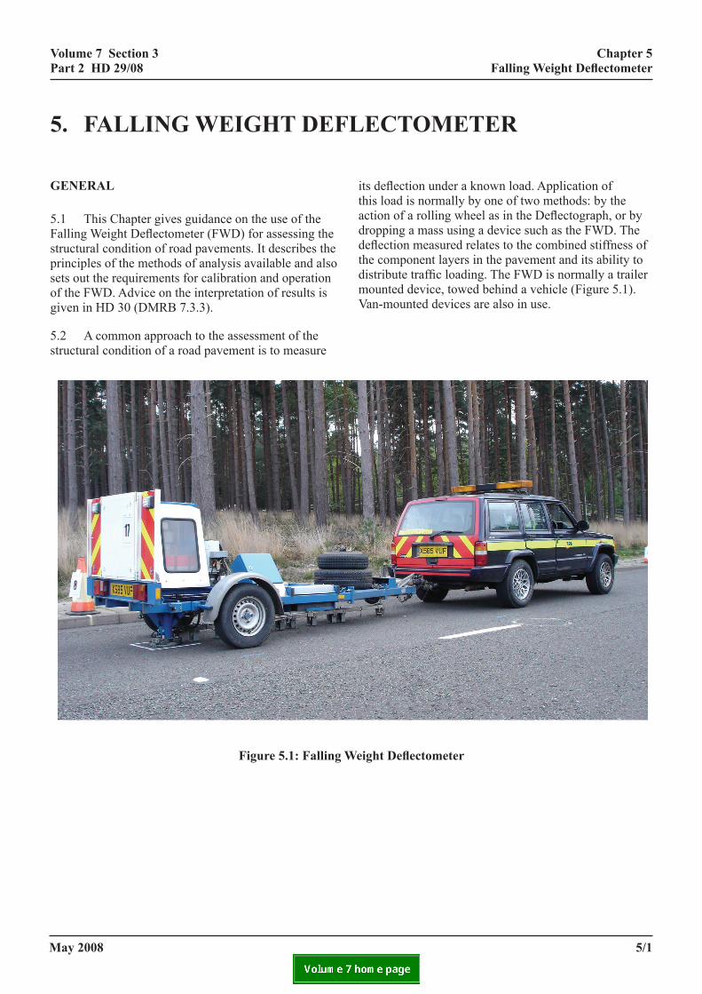
5.1 This Chapter gives guidance on the use of the Falling Weight Deflectometer (FWD) for assessing the structural condition of road pavements. It describes the principles of the methods of analysis available and also sets out the requirements for calibration and operation of the FWD. Advice on the interpretation of results is given in HD 30 (DMRB 7.3.3).
5.2 A common approach to the assessment of the structural condition of a road pavement is to measure
Figure 5.1: Falling W
may 2008
its deflection under a known load. Application of this load is normally by one of two methods: by the action of a rolling wheel as in the Deflectograph, or by dropping a mass using a device such as the FWD. The deflection measured relates to the combined stiffness of the component layers in the pavement and its ability to distribute traffic loading. The FWD is normally a trailer mounted device, towed behind a vehicle (Figure 5.1). Van-mounted devices are also in use.
5/1

volume 7 section 3 part 2 Hd 29/08
chapter 5 Falling Weight Deflectometer
5.3 The current policy for strength testing of flexible pavements described in this Part and in HD 30 (DMRB 7.3.3), requires that deflection is measured with a Deflectograph. The associated Deflection Design Method enables the residual life of the pavement to be predicted and strengthening overlays to be designed to extend that life. For rigid pavements, the assessment of structural maintenance requirements currently depends solely on Visual Condition Surveys (VCS). The FWD can provide additional detailed information on the structural condition of flexible and rigid pavements.
5.4 The impact method of load application used by the FWD is fundamentally different from the rolling wheel system employed by the Deflectograph. As yet, no satisfactory relationship has been found to convert FWD deflections to equivalent Deflectograph deflections so they cannot be input to the Overseeing Organisation’s design method. Whereas the Deflectograph system normally only uses the maximum deflection recorded at each measurement point, FWD measurements allow the deflected shape of the pavement surface to be derived. Estimates of layer stiffness can be made from knowledge of this deflected shape and the layer thicknesses.
5.5 There are many different methods of analyzing FWD measurements. Although these can produce relatively consistent results for layer stiffness, there is currently no standard approach for estimating residual life or overlay thickness using FWD results. The analytical process is subjective and calculating standard wheel load strains in the pavement and using these in conjunction with strain/fatigue life relationships is unreliable. The high sensitivity of the fatigue relationships used in this process can produce very different residual lives for the same data, when analysed by different engineers.
5.6 For the HA network the FWD must only be used for the following purposes:
a) to assess the stiffness of pavement layers of all pavement types;
b) to determine the load transfer efficiency across joints and cracks in rigid pavements.
These two types of surveys require the FWD to be configured differently and the results to be analysed in a completely different way. FWD data must not be used in isolation to other pavement condition indicators; it is important to characterise the
5/2
material properties and understand the pavement deterioration mechanisms (see HD 30 DMRB 7.3.3).
surveYs
5.7 Surveys may be commissioned for the specific purposes described in paragraph 5.6. They must be carried out on whole lengths, or sample lengths, of the road in need of structural maintenance, as identified by approved assessment methods, and on sample sections in sound condition to enable comparisons to be made. Advice on aspects to be considered when drawing up a survey specification are given below.
measuring equipment
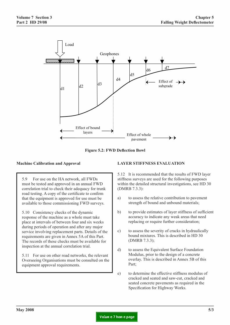
5.8 In principle the FWD generates a load pulse by dropping a mass onto a spring system. The mass and drop height can be adjusted to achieve the desired impact loading. Peak vertical deflections are measured at the centre of the loading plate and at several radial positions by a series of geophones. Figure 5.2 shows a typical deflection bowl (with the FWD configured for evaluating layer stiffness). These deflections and the peak impact load are stored electronically.
may 2008
volume 7 section 3 part 2 Hd 29/08
chapter 5 Falling Weight Deflectometer
Volume 7 Section 3 Chapter 5 Falling Weight Deflectometer
Figure 5.2: FWD D
machine calibration and approval
5.9 For use on the HA network, all FWDs must be tested and approved in an annual FWD correlation trial to check their adequacy for trunk road testing. A copy of the certificate to confirm that the equipment is approved for use must be available to those commissioning FWD surveys.
5.10 Consistency checks of the dynamic response of the machine as a whole must take place at intervals of between four and six weeks during periods of operation and after any major service involving replacement parts. Details of the requirements are given in Annex 5A of this Part. The records of these checks must be available for inspection at the annual correlation trial.
5.11 For use on other road networks, the relevant Overseeing Organisations must be consulted on the equipment approval requirements.
Part 2 HD 29/08
Figure 5.2 FWD
Machine Calibration and Approval
5.9 For use on the HA network, all FWDs must be testcheck their adequacy for trunk road testing. A copy of thuse must be available to those commissioning FWD surv
5.10 Consistency checks of the dynamic response of thebetween four and six weeks during periods of operation aDetails of the requirements are given in Annex 5A of thisinspection at the annual correlation trial.
5.11 For use on other road networks, the relevant Oversapproval requirements.
LAYER STIFFNESS EVALUATION
5.12 It is recommended that the results of FWD layer stthe detailed structural investigations, see HD 30 (DMRB
a) To assess the relative contribution to pavement stre
b) To provide estimates of layer stiffness of sufficientor require further consideration;
c) To assess the severity of cracks in hydraulically bo
Load
d2 d3 d1
Geophone
d
Effect of bound layers
may 2008
January 2008
d) To assess the Equivalent Surface Foundation Modescribed in Annex 5B of this Part;
eflection Bowl
laYer stiffness evaluation
5.12 It is recommended that the results of FWD layer stiffness surveys are used for the following purposes within the detailed structural investigations, see HD 30 (DMRB 7.3.3):
a) to assess the relative contribution to pavement strength of bound and unbound materials;
b) to provide estimates of layer stiffness of sufficient accuracy to indicate any weak areas that need replacing or require further consideration;
c) to assess the severity of cracks in hydraulically bound mixtures. This is described in HD 30 (DMRB 7.3.3);
d) to assess the Equivalent Surface Foundation Modulus, prior to the design of a concrete overlay. This is described in Annex 5B of this Part;
e) to determine the effective stiffness modulus of cracked and seated and saw-cut, cracked and seated concrete pavements as required in the Specification for Highway Works.
Deflection Bowl
ed and approved in an annual FWD correlation trial to e certificate to confirm that the equipment is approved for eys.
machine as a whole must take place at intervals of nd after any major service involving replacement parts. Part. The records of these checks must be available for
eeing Organisations must be consulted on the equipment
iffness surveys are used for the following purposes within 7.3.3):
ngth of bound and unbound materials;
accuracy to indicate any weak areas that need replacing
und mixtures. This is described in HD 30 (DMRB 7.3.3);
dulus, prior to the design of a concrete overlay. This is
s
4 d5
d6 d7
Effect of whole pavement
Effect of subgrade
5/3
5/3
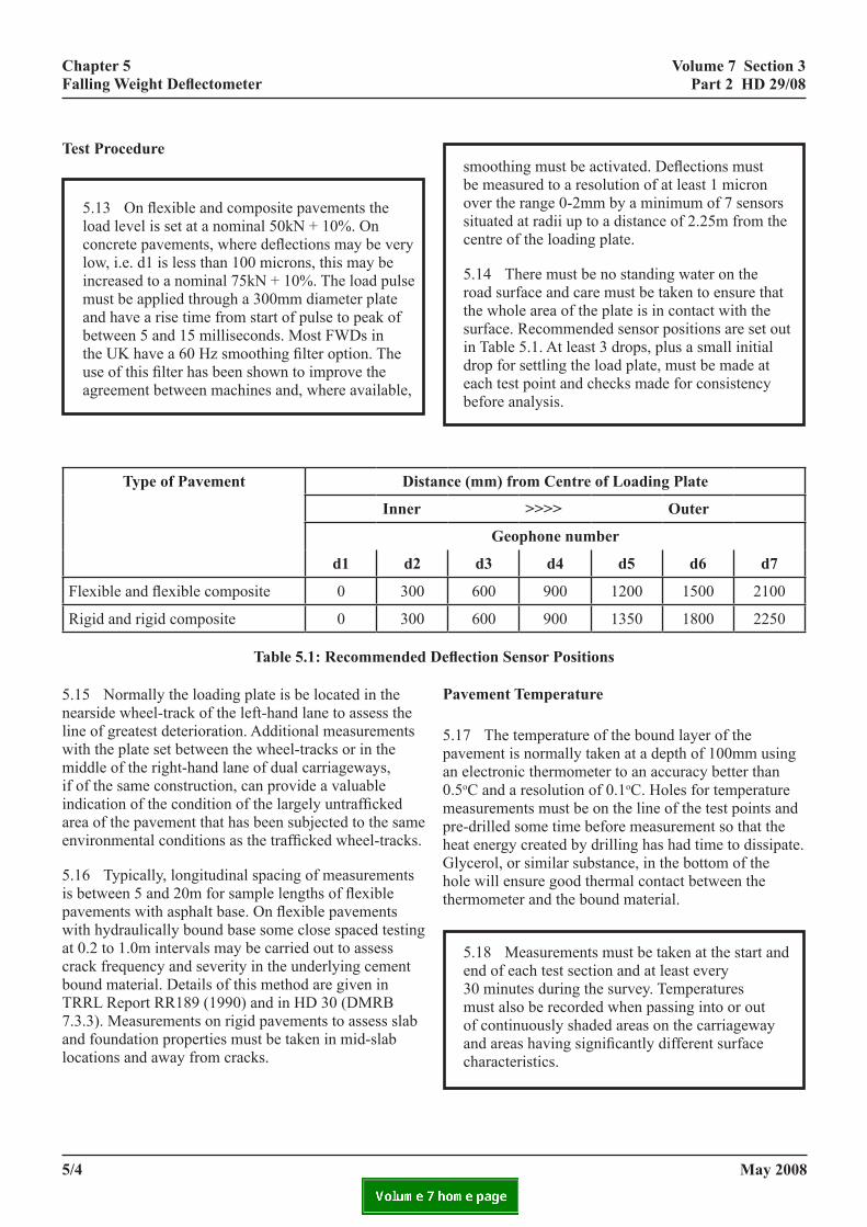
volume 7 section 3 part 2 Hd 29/08
chapter 5 Falling Weight Deflectometer
test procedure
5.13 On flexible and composite pavements the load level is set at a nominal 50kN + 10%. On concrete pavements, where deflections may be very low, i.e. d1 is less than 100 microns, this may be increased to a nominal 75kN + 10%. The load pulse must be applied through a 300mm diameter plate and have a rise time from start of pulse to peak of between 5 and 15 milliseconds. Most FWDs in the UK have a 60 Hz smoothing filter option. The use of this filter has been shown to improve the agreement between machines and, where available,
type of pavement Dista
inner
d1 d2
Flexible and flexible composite 0 300
Rigid and rigid composite 0 300
Table 5.1: Recommended D
5.15 Normally the loading plate is be located in the nearside wheel-track of the left-hand lane to assess the line of greatest deterioration. Additional measurements with the plate set between the wheel-tracks or in the middle of the right-hand lane of dual carriageways, if of the same construction, can provide a valuable indication of the condition of the largely untrafficked area of the pavement that has been subjected to the same environmental conditions as the trafficked wheel-tracks.
5.16 Typically, longitudinal spacing of measurements is between 5 and 20m for sample lengths of flexible pavements with asphalt base. On flexible pavements with hydraulically bound base some close spaced testing at 0.2 to 1.0m intervals may be carried out to assess crack frequency and severity in the underlying cement bound material. Details of this method are given in TRRL Report RR189 (1990) and in HD 30 (DMRB 7.3.3). Measurements on rigid pavements to assess slab and foundation properties must be taken in mid-slab locations and away from cracks.
5/4
smoothing must be activated. Deflections must be measured to a resolution of at least 1 micron over the range 0-2mm by a minimum of 7 sensors situated at radii up to a distance of 2.25m from the centre of the loading plate.
5.14 There must be no standing water on the road surface and care must be taken to ensure that the whole area of the plate is in contact with the surface. Recommended sensor positions are set out in Table 5.1. At least 3 drops, plus a small initial drop for settling the load plate, must be made at each test point and checks made for consistency before analysis.
nce (mm) from Centre of Loading Plate
>>>> outer
geophone number
d3 d4 d5 d6 d7
600 900 1200 1500 2100
600 900 1350 1800 2250
eflection Sensor Positions
pavement temperature
5.17 The temperature of the bound layer of the pavement is normally taken at a depth of 100mm using an electronic thermometer to an accuracy better than 0.5oC and a resolution of 0.1oC. Holes for temperature measurements must be on the line of the test points and pre-drilled some time before measurement so that the heat energy created by drilling has had time to dissipate. Glycerol, or similar substance, in the bottom of the hole will ensure good thermal contact between the thermometer and the bound material.
5.18 Measurements must be taken at the start and end of each test section and at least every 30 minutes during the survey. Temperatures must also be recorded when passing into or out of continuously shaded areas on the carriageway and areas having significantly different surface characteristics.
may 2008
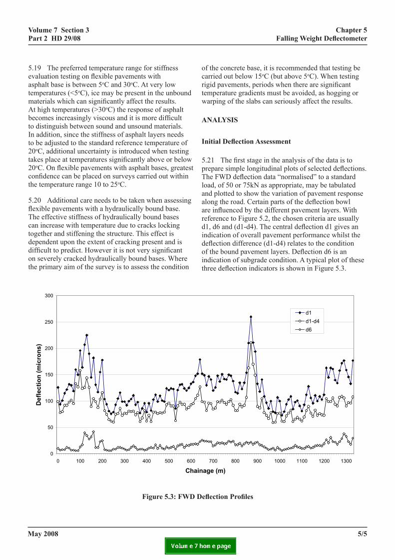
volume 7 section 3 part 2 Hd 29/08
chapter 5 Falling Weight Deflectometer
Deflection Profiles
700 800 900 1000 1100 1200 1300
inage (m)
Deflection Profiles
n the type and condition of the material present, such plots
5.19 The preferred temperature range for stiffness evaluation testing on flexible pavements with asphalt base is between 5oC and 30oC. At very low temperatures (<5oC), ice may be present in the unbound materials which can significantly affect the results. At high temperatures (>30oC) the response of asphalt becomes increasingly viscous and it is more difficult to distinguish between sound and unsound materials. In addition, since the stiffness of asphalt layers needs to be adjusted to the standard reference temperature of 20oC, additional uncertainty is introduced when testing takes place at temperatures significantly above or below 20oC. On flexible pavements with asphalt bases, greatest confidence can be placed on surveys carried out within the temperature range 10 to 25oC.
5.20 Additional care needs to be taken when assessing flexible pavements with a hydraulically bound base. The effective stiffness of hydraulically bound bases can increase with temperature due to cracks locking together and stiffening the structure. This effect is dependent upon the extent of cracking present and is difficult to predict. However it is not very significant on severely cracked hydraulically bound bases. Where the primary aim of the survey is to assess the condition
Figure 5.3: FWD
Chapter 5 Falling Weight Deflectometer
0
50
100
150
200
250
300
0 100 200 300 400 500 600
Cha
Def
lect
ion
(mic
rons
)
Figure 5.3 FWD
5.22 Although actual values of deflection will depend o
may 2008
5/6
will show relative differences in the condition of the layeidentified and give an indication of where structural wea
Cracks in Hydraulically Bound Mixtures
5.23 Results of tests on bases formed from hydraulicallenable the spacing and severity of primary transverse craThe crack spacing is a function of the age and strength ostronger material. Guidance on interpretation of such me
Calculating Layer Stiffnesses
5.24 The deflected shape of the surface, generated by acondition of the construction layers. Computer programsmodel the pavement structure. Essentially this analysis iswhich predicts the surface deflection under a given appliis used to match the computed deflections to the measureuntil a reasonable match is obtained.
5.25 There are a number of different programs availablstiffness estimates of pavement layers. The results of theused and the way in which the pavement is modelled (incproperties of those layers). For this reason, the followingperforming back-analysis for the HA’s network. The useconsistent results independent of who is performing the aanalysis procedures may be required but their use must bstandard procedure.
Back-analysis program
of the concrete base, it is recommended that testing be carried out below 15oC (but above 5oC). When testing rigid pavements, periods when there are significant temperature gradients must be avoided, as hogging or warping of the slabs can seriously affect the results.
analYsis
Initial Deflection Assessment
5.21 The first stage in the analysis of the data is to prepare simple longitudinal plots of selected deflections. The FWD deflection data “normalised” to a standard load, of 50 or 75kN as appropriate, may be tabulated and plotted to show the variation of pavement response along the road. Certain parts of the deflection bowl are influenced by the different pavement layers. With reference to Figure 5.2, the chosen criteria are usually d1, d6 and (d1-d4). The central deflection d1 gives an indication of overall pavement performance whilst the deflection difference (d1-d4) relates to the condition of the bound pavement layers. Deflection d6 is an indication of subgrade condition. A typical plot of these three deflection indicators is shown in Figure 5.3.Volume 7 Section 3
Part 2 HD 29/08
d1d1-d4d6
5/5
January 2008
rs, enable lengths of road with similar behaviour to be kness may be present.
y bound mixtures showing peaks in the central deflection cks to be determined even if not visible on the surface. f the cement bound material, a wider spacing indicating a asurements is given in HD 30 (DMRB 7.3.3).
n FWD impact load, depends upon the type, thickness and using linear elastic multi-layered analysis can be used to based on a mathematical model of the pavement structure ed load. An iterative procedure known as “back-analysis” d values. The layer stiffnesses are adjusted in this process
e for performing back-analysis of FWD data to produce analysis are strongly influenced by the type of program luding the number of layers used and the assumed back-analysis procedure must be followed whenever of this procedure is expected to produce reasonably nalysis. There will be occasions where alternative back-e clearly justified and they must be used in addition to the
volume 7 section 3 part 2 Hd 29/08
chapter 5 Falling Weight Deflectometer
5.22 Although actual values of deflection will depend on the type and condition of the material present, such plots will show relative differences in the condition of the layers, enable lengths of road with similar behaviour to be identified and give an indication of where structural weakness may be present.
cracks in Hydraulically Bound mixtures
5.23 Results of tests on bases formed from hydraulically bound mixtures showing peaks in the central deflection enable the spacing and severity of primary transverse cracks to be determined even if not visible on the surface. The crack spacing is a function of the age and strength of the cement bound material, a wider spacing indicating a stronger material. Guidance on interpretation of such measurements is given in HD 30 (DMRB 7.3.3).
calculating layer stiffnesses
5.24 The deflected shape of the surface, generated by an FWD impact load, depends upon the type, thickness and condition of the construction layers. Computer programs using linear elastic multi-layered analysis can be used to model the pavement structure. Essentially this analysis is based on a mathematical model of the pavement structure which predicts the surface deflection under a given applied load. An iterative procedure known as “back-analysis” is used to match the computed deflections to the measured values. The layer stiffnesses are adjusted in this process until a reasonable match is obtained.
5.25 There are a number of different programs available for performing back-analysis of FWD data to produce stiffness estimates of pavement layers. The results of the analysis are strongly influenced by the type of program used and the way in which the pavement is modelled (including the number of layers used and the assumed properties of those layers). For this reason, the following back-analysis procedure must be followed whenever performing back-analysis for the HA’s network. The use of this procedure is expected to produce reasonably consistent results independent of who is performing the analysis. There will be occasions where alternative back-analysis procedures may be required but their use must be clearly justified and they must be used in addition to the standard procedure.
B
p
5/6
1 The general theory of stresses and displacements in layered s1945.
ack-Analysis Program
5.26 For use on the HA’s network, the back-analysis program must comply with the following criteria:
i. it must model the pavement structure as a number of horizontally infinite linear elastic layers;
ii. it must use elastic multi-layer analysis based on Burmister’s equations1 with all layers modelled linearly including an infinite depth subgrade and no slip between layers;
iii. it must be able to model at least three independent layers;
iv. it must be able to handle at least seven deflection sensors;
v. it must be able to report the computed surface deflection values.
avement model
5.27 For the HA’s network, the following rules must be applied when determining how to model the pavement:
i. the minimum thickness of any single layer must be 75mm;
ii. the maximum number of independent layers (including the subgrade) must be three;
iii. asphalt layers must be combined and modelled as a single layer;
iv. concrete layers must be combined and modelled as a single layer;
v. where an asphalt layer overlies a concrete layer, these must be modelled as separate layers provided that neither is less than one-third the thickness of the other (subject to constraints i and ii);
may 2008
oil systems. Burmister. Journal of applied physics, Volume 16,
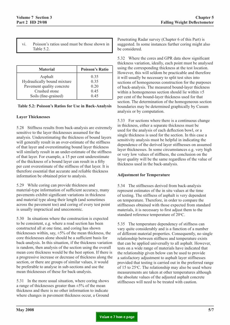
volume 7 section 3 part 2 Hd 29/08
chapter 5 Falling Weight Deflectometer
vi. Poisson’s ratios used must be those shown in Table 5.2.
material poisson’s ratio
Asphalt Hydraulically bound mixture Pavement quality concrete
Crushed stone Soils (fine-grained)
0.35 0.35 0.20 0.45 0.45
Table 5.2: Poisson’s Ratios for Use in Back-Analysis
layer thicknesses
5.28 Stiffness results from back-analysis are extremely sensitive to the layer thicknesses assumed for the analysis. Underestimating the thickness of bound layers will generally result in an over-estimate of the stiffness of that layer and overestimating bound layer thickness will similarly result in an under-estimate of the stiffness of that layer. For example, a 15 per cent underestimate of the thickness of a bound layer can result in a fifty per cent overestimate of the stiffness of that layer. It is therefore essential that accurate and reliable thickness information be obtained prior to analysis.
5.29 While coring can provide thickness and material-type information of sufficient accuracy, many pavements exhibit significant variations in thickness and material type along their length (and sometimes across the pavement too) and coring of every test point is usually impractical and uneconomic.
5.30 In situations where the construction is expected to be consistent, e.g. where a road section has been constructed all at one time, and coring has shown thicknesses within, say, ±5% of the mean thickness, the core thicknesses alone should be a sufficient basis for back-analysis. In this situation, if the thickness variation is random, then analysis of the section using the overall mean core thickness would be the best option. If there is a progressive increase or decrease of thickness along the section, or there are groups of similar values, it would be preferable to analyse in sub-sections and use the mean thicknesses of these for back-analysis.
5.31 In the more usual situation, where coring shows a range of thicknesses greater than ±5% of the mean thickness and there is no other information to indicate where changes in pavement thickness occur, a Ground
Psube
5.thusHitseofwpeseboan
5.inussisedelaorlath
a
5.reofonstmst
5.vaofrethtetha profmthst
may 2008
enetrating Radar survey (Chapter 6 of this Part) is ggested. In some instances further coring might also considered.
32 Where the cores and GPR data show significant ickness variation, ideally, each point must be analysed ing the corresponding thickness at the test location. owever, this will seldom be practicable and therefore will usually be necessary to split test sites into ctions of homogeneous construction for the purposes back-analysis. The measured bound-layer thickness ithin a homogeneous section should lie within ±5 r cent of the bound-layer thickness used for that ction. The determination of the homogeneous section undaries may be determined graphically by Cusum alysis or by computation.
33 For sections where there is a continuous change thickness, either a separate thickness must be ed for the analysis of each deflection bowl, or a ngle thickness is used for the section. In this case a nsitivity analysis must be helpful in indicating the pendence of the derived layer stiffnesses on assumed yer thicknesses. In some circumstances e.g. very high very low values of stiffness, the conclusion on the yer quality will be the same regardless of the value of ickness used in the back-analysis.
djustment for temperature
34 The stiffnesses derived from back-analysis present estimates of the in situ values at the time testing. The stiffness of asphalt is very dependent temperature. Therefore, in order to compare the
iffnesses obtained with those expected from standard aterials, it is necessary to first adjust them to the andard reference temperature of 20oC.
35 The temperature dependency of stiffness can ry quite considerably and is a function of a number different material properties. Consequently, no single lationship between stiffness and temperature exists at can be applied universally to all asphalt. However, sts on a wide range of materials have indicated that e relationship given below can be used to provide satisfactory adjustment to asphalt layer stiffnesses ovided that testing is carried out in the preferred range 15 to 25oC. The relationship may also be used where easurements are taken at other temperatures although e absolute values of the adjusted asphalt concrete iffnesses will need to be treated with caution.
5/7

volume 7 section 3 part 2 Hd 29/08
chapter 5 Falling Weight Deflectometer
5.36 The temperature dependency of the stiffness of severely cracked asphalt tends to be far less than that of intact materials. Therefore, where a layer is known to be severely cracked throughout its depth, temperature adjustment should not normally be applied.
5.37 For use on the HA’s network, the stiffness of asphalt layers, unless severely cracked, must be adjusted to the standard reference temperature of 20oC using the following relationship:
E20 = ET .10(0.0003 x (20-T)² - 0.022 x (20-T))
Where: E20 = Stiffness at 20oC; ET = Stiffness at temperature T ;
T = Temperature of the asphalt at the time of testing (measured at 100mm depth).
goodness of fit
5.38 There are two goodness of fit parameters that are commonly used for indicating how well the program has matched the data. These are the Absolute Mean Deviation (AMD) and the Root Mean Squared Deviation (RMS), defined as:
Absolute Mean Deviation (AMD) = |∑(dci - dmi)/n|
Root Mean Squared Deviation (RMS) = √(∑(dci - dmi)
2/n)
Where: dmi are the measured deflections in microns at positions i =1 to n;
dci are the calculated deflections in microns at positions i =1 to n;
n is the total number of sensor positions used in the analysis (normally seven).
The AMD indicates whether or not there is an overall bias to the calculated deflection bowl relative to the measured bowl. The RMS indicates how well, on average, the calculated bowl matches the measured bowl. Although a good fit does not in itself indicate that a correct solution has been obtained, a poor fit does indicate that the solution found is suspect.
5.39 Different back-analysis programs vary in their ability to match calculated to measured deflections. Poor fits can also be obtained where cracks or other
5/8
discontinuities are present in the pavement, where incorrect assumptions about layer thicknesses or material types are made, or where layer de-bonding is present. In addition, increasing the number of layers improves the level of fit. Table 5.3 contains guide values for AMD and RMS for pavements modelled with two or three layers. Bowls for which the AMD or RMS exceed these values must be treated with caution. Isolated results which exceed these limits must be discounted when assessing the overall condition of a section.
number of layers maximum values (microns)
amd rms
2 4 11
3 2 5
table 5.3: guide values for goodness of fit
ALTERNATIVE BACK-ANALYSIS APPROACHES
5.40 There will be occasions where the standard back-analysis procedure may not produce the most representative estimates of stiffness and an alternative analysis technique may be more appropriate. Table 5.4 lists some example scenarios where alternative techniques may be appropriate. Where an alternative back-analysis method is used, it needs to be performed in addition to the standard procedure and both analyses need to be reported.
may 2008
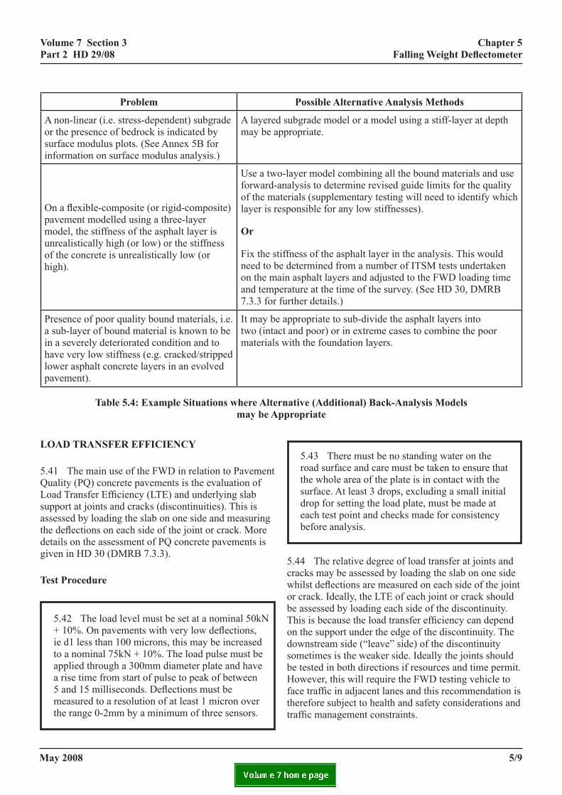
volume 7 section 3 part 2 Hd 29/08
chapter 5 Falling Weight Deflectometer
problem
A non-linear (i.e. stress-dependent) subgrade or the presence of bedrock is indicated by surface modulus plots. (See Annex 5B for information on surface modulus analysis.)
A layered sumay be app
On a flexible-composite (or rigid-composite) pavement modelled using a three-layer model, the stiffness of the asphalt layer is unrealistically high (or low) or the stiffness of the concrete is unrealistically low (or high).
Use a two-lforward-anaof the materlayer is resp
or
Fix the stiffneed to be don the mainand tempera7.3.3 for fur
Presence of poor quality bound materials, i.e. a sub-layer of bound material is known to be in a severely deteriorated condition and to have very low stiffness (e.g. cracked/stripped lower asphalt concrete layers in an evolved pavement).
It may be aptwo (intact materials w
Table 5.4: Example Situations where Alternmay be app
load transfer efficiencY
5.41 The main use of the FWD in relation to Pavement Quality (PQ) concrete pavements is the evaluation of Load Transfer Efficiency (LTE) and underlying slab support at joints and cracks (discontinuities). This is assessed by loading the slab on one side and measuring the deflections on each side of the joint or crack. More details on the assessment of PQ concrete pavements is given in HD 30 (DMRB 7.3.3).
test procedure
5.42 The load level must be set at a nominal 50kN + 10%. On pavements with very low deflections, ie d1 less than 100 microns, this may be increased to a nominal 75kN + 10%. The load pulse must be applied through a 300mm diameter plate and have a rise time from start of pulse to peak of between 5 and 15 milliseconds. Deflections must be measured to a resolution of at least 1 micron over the range 0-2mm by a minimum of three sensors.
5cwobTodsbHftt
may 2008
possible alternative analysis methods
bgrade model or a model using a stiff-layer at depth ropriate.
ayer model combining all the bound materials and use lysis to determine revised guide limits for the quality ials (supplementary testing will need to identify which onsible for any low stiffnesses).
ness of the asphalt layer in the analysis. This would etermined from a number of ITSM tests undertaken asphalt layers and adjusted to the FWD loading time ture at the time of the survey. (See HD 30, DMRB ther details.)
propriate to sub-divide the asphalt layers into and poor) or in extreme cases to combine the poor ith the foundation layers.
ative (Additional) Back-Analysis Models ropriate
5.43 There must be no standing water on the road surface and care must be taken to ensure that the whole area of the plate is in contact with the surface. At least 3 drops, excluding a small initial drop for setting the load plate, must be made at each test point and checks made for consistency before analysis.
.44 The relative degree of load transfer at joints and racks may be assessed by loading the slab on one side hilst deflections are measured on each side of the joint r crack. Ideally, the LTE of each joint or crack should e assessed by loading each side of the discontinuity. his is because the load transfer efficiency can depend n the support under the edge of the discontinuity. The ownstream side (“leave” side) of the discontinuity ometimes is the weaker side. Ideally the joints should e tested in both directions if resources and time permit. owever, this will require the FWD testing vehicle to
ace traffic in adjacent lanes and this recommendation is herefore subject to health and safety considerations and raffic management constraints.
5/9
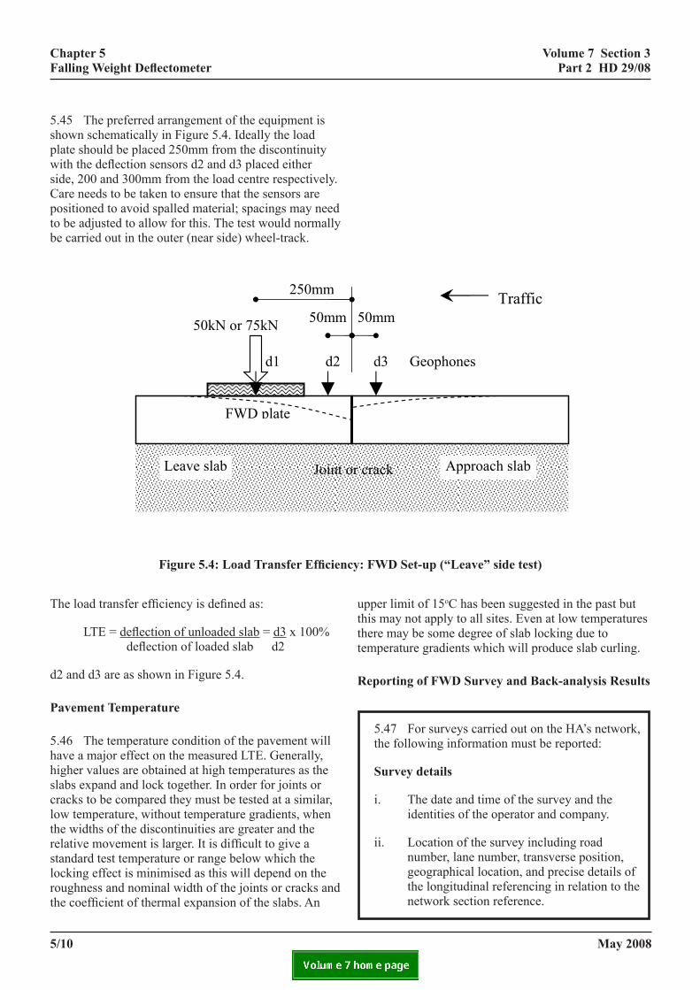
volume 7 section 3 part 2 Hd 29/08
chapter 5 Falling Weight Deflectometer
Volume 7 Section 3 Chapter 5 Part 2 HD 29/08 Falling Weight Deflectometer
Ja
5.44 The relative degree of load transfer at joints and cracks may be assessed by loading the slab on one side whilst deflections are measured on each side of the joint or crack. Ideally, the LTE of each joint or crack must be assessed by loading each side of the discontinuity. This is because the load transfer efficiency can depend on the support under the edge of the discontinuity. The downstream side (“leave” side) of the discontinuity sometimes is the weaker side. Ideally the joints must be tested in both directions if resources and time permit. However, this will req nt lanes and this recommendation is therefore subject to he t constraints.
5.4 own schematically in Figure 5.4. Ideally the load plate sh e deflection sensors d2 and d3 placed either side, 200 and 30 be taken to ensure that the sensors are positioned to avoid sp llow for this. The test would normally be carried out in the ou
Th
d2
Pa
5.4 higher va o be co of the dis ure or ran f the joi ested in king du
50mm
d3 Geophones
Traffic
5.45 The preferred arrangement of the equipment is shown schematically in Figure 5.4. Ideally the load plate should be placed 250mm from the discontinuity with the deflection sensors d2 and d3 placed either side, 200 and 300mm from the load centre respectively. Care needs to be taken to ensure that the sensors are positioned to avoid spalled material; spacings may need to be adjusted to allow for this. The test would normally be carried out in the outer (near side) wheel-track.
Figure 5.4: Load Transfer Efficien
The load transfer efficiency is defined as:
LTE = deflection of unloaded slab = d3 x 100% deflection of loaded slab d2
d2 and d3 are as shown in Figure 5.4.
pavement temperature
5.46 The temperature condition of the pavement will have a major effect on the measured LTE. Generally, higher values are obtained at high temperatures as the slabs expand and lock together. In order for joints or cracks to be compared they must be tested at a similar, low temperature, without temperature gradients, when the widths of the discontinuities are greater and the relative movement is larger. It is difficult to give a standard test temperature or range below which the locking effect is minimised as this will depend on the roughness and nominal width of the joints or cracks and the coefficient of thermal expansion of the slabs. An
uire the FWD testing vehicle to face traffic in adjacealth and safety considerations and traffic managemen
5 The preferred arrangement of the equipment is should be placed 250mm from the discontinuity with th0mm from the load centre respectively. Care needs toalled material; spacings may need to be adjusted to ater (near side) wheel-track.
Figure 5.4 Load Transfer Efficie
e load transfer efficiency is defined as:
LTE = deflection of unloaded slab = deflection of loaded slab
and d3 are as shown in Figure 5.4.
vement Temperature
6 The temperature condition of the pavement will lues are obtained at high temperatures as the slabs exmpared they must be tested at a similar, low temperacontinuities are greater and the relative movement isge below which the locking effect is minimised as thnts or cracks and the coefficient of thermal expansiothe past but this may not apply to all sites. Even at loe to temperature gradients which will produce slab c
250mm
50mm
Joint
50kN or 75kN
d2
FWD plate
d1
Leave slab
5/10
nuary 2008
cy: FWD Set-up (“Leave” side test)
upper limit of 15oC has been suggested in the past but this may not apply to all sites. Even at low temperatures there may be some degree of slab locking due to temperature gradients which will produce slab curling.
Reporting of FWD Survey and Back-analysis Results
5.47 For surveys carried out on the HA’s network, the following information must be reported:
survey details
i. The date and time of the survey and the identities of the operator and company.
ii. Location of the survey including road number, lane number, transverse position, geographical location, and precise details of the longitudinal referencing in relation to the network section reference.
ncy: FWD Set-up (“Leave” side test)
d3 x 100% d2
have a major effect on the measured LTE. Generally,pand and lock together. In order for joints or cracks tture, without temperature gradients, when the widths larger. It is difficult to give a standard test temperatis will depend on the roughness and nominal width o
n of the slabs. An upper limit of 15oC has been suggw temperatures there may be some degree of slab locurling.
or crack Approach slab
may 2008
5/11

volume 7 section 3 part 2 Hd 29/08
chapter 5 Falling Weight Deflectometer
iii. Make, model and serial number of the FWD used.
iv. The mass of the falling weight and the diameter of the loading plate.
v. Type, number and positions of the geophones.
vi. Locations, depths (should be 100mm) and times of pavement temperatures recorded during the survey.
vii. Test type, leave or approach for Load Transfer Efficiency (LTE).
viii. “Supplementary” and “F20” files to be provided for loading into the Highways Agency Pavement Management System (HAPMS), for all trunk road surveys.
survey results
i. Tabulated deflections (normalised to 50kN or 70kN as appropriate).
ii. Graphs of the deflection parameters d1, (d1-d4) and d6 (normalised to 50 or 75kN as appropriate).
iii. Temperature applicable to each test point.
analysis details
i. Details of the FWD back-analysis program used (name, version, mode of operation).
ii. Details of the model used (thicknesses for each layer, number of layers, type of material assumed, details of the source of the construction information used e.g. cores, GPR, as-built drawings etc.).
analysis results
i. Tabulated back-analysed stiffnesses (including “as measured” and “adjusted to 20oC” for asphalt layers).
ii. Graphs of the layer stiffness results (asphalt layers adjusted to 20oC).
i
i
5uaeaiwm
Lig
5.49devlayeare
may 2008
ii. Tabulated layer thicknesses used for the analysis (i.e. for each test point).
v. AMD and RMS values for each test point.
.48 The template given in Annex 5B must be sed to record the details. Where an alternative nalysis is used, the report must include a clear xplanation of the reason for using the additional nalysis. Both sets of analyses must be presented n the format specified and it must be made clear hich set of results relates to which analysis ethod.
htweight Devices
Lightweight dynamic plate or falling weight ices are also useful for testing foundation (unbound) rs. Their use is more limited than the FWD and they not to be used for overall pavement assessment.
5/11
volume 7 section 3 part 2 Hd 29/08
ADAR
chapter 6 ground-Penetrating Radar
6. gROUND-PENETRATINg R
introduction
general
6.1 Ground-penetrating radar (GPR) is a non-destructive tool that can be used to obtain information about the construction of a pavement and its internal features. This information can be used to enhance pavement condition information obtained from visual condition, deflection surveys, coring and trial pits.
6.2 Typically, GPR can provide information about changes in pavement construction, layer thicknesses and defects/features within the pavement. The quality of the information obtained from ground radar is largely a function of three factors:
• the electrical properties (dielectric constant and the conductivity) of the materials forming the pavement;
• the type of GPR equipment employed;
• the processing software and analysis methodology including calibration procedures employed.
scope
6.3 This Part gives guidance on the appropriate use of GPR on paved roads only and does not cover the monitoring of services such as subsurface drains, buried pipes and any other non-pavement related features. The advice sets out the requirements for successful operation of a GPR survey, for quality control of the survey, and for the presentation of results.
6.4 Guidance on the use of GPR in connection with the assessment of highway structures is given in BA 86 (DMRB 3.1.7).
legislation
6.5 Section 1(1) of Wireless Telegraphy Act 1949, makes it an offence for any person to operate any equipment for wireless telegraphy if not used in accordance with the license granted
US
gen
6.6 theiPar
loc
rec
6.8 idenrobthe survclasaccin Tconreli
may 2008
by the Office of Communications (OFCOM). All GPR operators operating in the UK must hold an OFCOM license and operate as required in respect of the EuroGPR Code of Good Practice. Also, the use of GPR on roads near radio astronomy sites requires specific permission from OFCOM.
E OF gROUND-PENETRATINg RADAR
eral Principles of ground-Penetrating Radar
The general principles of the use of GPR and r antenna types are explained in Annex 6A of this t.
ation referencing
6.7 Accurate location referencing is fundamental to the collection of good quality ground-penetrating radar data particularly as thicknesses will have to be calibrated or checked against pavement cores. All GPR surveys carried out on the HA network must be referenced against network sections to an accuracy of better than ± 5m.
If the surveys are carried out at traffic speed then particular care will need to taken to achieve the above requirement, the use of an automatic location referencing system may well be needed such as a sophisticated GPS and inertial guidance system as used with TRACS.
ommended uses
GPR systems available at present are able to tify pavement features to differing degrees of
ustness for assessment purposes depending on feature and the survey speed. The ability of GPR eys to identify pavement features are therefore sified into four classes A to D, depending on how urately and reliably they can be identified; as shown able 6.1. Surveys with the classification A are sidered routine and have sufficient accuracy and ability to be used regularly for pavement assessment.
6/1
volume 7 section 3 part 2 Hd 29/08
chapter 6 ground-Penetrating Radar
Surveys with the classification B are considered to be suitable for Confirmation that this pavement condition exists with the assistance of evidence from other techniques. Surveys with the classification C should only be used with caution as a guide and together with other data to indicate the possible construction or condition of the pavement. Surveys with the classification D are unproven and have yet to be demonstrated as suitable for use on the network. Table 6.1 also gives the constraints and other requirements when utilising GPR to ascertain a specific pavement feature. Ongoing developments in GPR systems make it likely that more features will be detected accurately and reliably in future. This advice on the limitations of the technique will be kept under review and any significant developments will be incorporated when they are ready for implementation.
6.9 The sampling rate of a GPR system influences the size of feature that can be detected and the sampling rate depends largely on the survey speed of the equipment amongst other parameters. This is mainly why surveys that detect discrete features in the pavement, such as voids or cracks, have been given different classifications in Table 6.1 depending on the survey speed. The surveys at slower speed, ie less than 30 km/h, will normally require appropriate traffic management. This subject is covered in more detail in Annex 6A in this Part.
6.10 It is recommended that surveys for the HA network be commissioned only if they meet the A and B level classifications as shown in Table 6.1 Further details of how GPR can be used to assess these pavement features are explained from paragraph 6.13 onwards.
6.11 It is also recommended that the GPR surveys should be undertaken prior to any coring to ensure that the core extraction occurs in homogeneous road sections.
limitations of use
6.12 GPR cannot penetrate metal, closely spaced reinforcement or highly conducting materials.
6.13 GPR surveys must not be carried out when it is raining or when standing water is present on the surface of the pavement. This is because a thick film of surface water may affect the radar signal making interpretation of the data more difficult. Calibration of the radar may also be less certain as explained in Annex 6B of this Part.
6/2
6.14 GPR surveys must not be carried out on salted (de-iced) roads in case there is significant penetration of salt water into the subsurface materials beneath the road. Salt increases the conductivity of the pavement materials and the transmission of ground radar signals is heavily dependent on the pavement’s conductivity. High conductivity will lead to an attenuation of the radar signal and therefore reduces considerably the depth of penetration of the radar.
Construction Changes (Class A)
6.15 The following are typical examples of changes of pavement constructions which GPR can detect:
• changes from hydraulically bound to asphalt base and vice versa;
• haunches;
• hidden trenches covered by bituminous surfacing.
However if the construction change is outside the line of the survey, such as haunch construction, or of a short length then the survey may not be able to detect the change.
6.16 Direct evidence of construction changes must be confirmed by coring. Ideally, this must be carried out after the GPR survey has been carried out at locations of homogeneous construction (determined from the GPR) and where the GPR interpretation is unclear.
may 2008

may 2008
volume 7 section 3
part 2 Hd
29/08pavement features Classification (see below) constraints and requirements
Slow speed <30km/h
Traffic speed >80km/h
Construction changes A A If the construction changes are outside the line of the survey or of a short length they may not be
ution is required for interpreting disintegrated lean te is 20mm (2.5GHz antenna). tection. For measurement at traffic speed, the e and the length of the voids. Depth of the feature curacy of measurements.r reliable detection. For measurement at traffic mpling rate and the length of the voids. Depth of ffect the accuracy of measurements.oint to assess dowel and tie bars. With a single d two further scans each side of the joint on a line e of survey will also allow the determination of re present. ture content. To eliminate uncertainty of data ry’ season when the sub base is likely to be in an ey carried out when the sub-base is deemed to be between the sub-base and the subgrade must be
erator and a slow survey speed are required. k depth measurements. No equipment available for
ining the signal attenuation, amplitude of onse from within the material, and automatically he material. However, the only certain way to
t slow speed with high frequency antenna, higher he debonded area.el but if the steel has corroded and damaged the e.d by reflections from the overlying reinforcement.
identify. Water filled voids less than 25mm deep
stems. Not proven to date.vement condition based on other data. ture research.
by gPR
chapter 6
ground-Penetrating R
adar
detected.Bound and unbound layer thicknesses and profiles
A A Low speed surveys needed for reinforced layers. Caconcrete layers. The best depth resolution for concre
Deep air-filled voids directly beneath unreinforced concrete slabs
B C Void depths need to be at least 80mm for reliable desuccess in detection will depend on the sampling ratand chosen antenna frequency will also affect the ac
Water-filled voids directly beneath unreinforced concrete slabs
B C Water-filled void depths need to be at least 25mm fospeed, the success in detection will depend on the sathe feature and chosen antenna frequency will also a
Depth and gross misalignment of joint dowel bars; detail of steel reinforcement in concrete slabs
B D Slow-speed scans are required along the line of the jantenna, one scan is required just beside the joint, anjust above the ends of the dowel or tie bars. This typthe depth and spacing of reinforcing steel mesh whe
Variation of sub-base moisture content (duplicate surveys required)
B C Signal velocity changes with material and with moisinterpretation, one survey must be carried out in a ‘dequilibrium moisture condition and an identical survwet (i.e. in the ‘wet’ season). Note that the interface visible in the signals for the technique to work.
Depths of surface cracks in fully flexible pavements
C D Specialised GPR equipment, a specifically trained opSample cores are required for calibration of the cractraffic speed survey.
Broad types of pavement materials C C Some idea of material type can be obtained by examreflections at material boundaries, continuity of respdetermined or self-calibrated signal velocity within tidentify materials is to use core data.
Debonding of pavement layers D D This feature might be visible in the bound material achance to be detected with the presence of water in t
Condition of steel in concrete D D Unlikely to indicate directly the condition of any stesurrounding concrete the radar may detect the damag
Voids and wet patches beneath reinforced concrete slabs
D D Reflections from voids or wet patches may be maske
Shallow voids directly beneath unreinforced concrete slabs
D D Air filled voids less than 80 mm deep are difficult toare also difficult to identify.
Debonding of joint sealant D D Might be detected at slow speed with special GPR syA - Sufficient accuracy and reliability to be used for pavement assessment. B - Use to confirm assessment of paC - Use with caution and as a guide, along with other data, to indicate possible D - Unproven and candidates for fuconstruction/condition of pavement.
Table 6.1: Accuracy and Reliability of Identification of Pavement Features
6/3
volume 7 section 3 part 2 Hd 29/08
chapter 6 ground-Penetrating Radar
Layer Thickness (Class A)
6.17 Correct interpretation of deflection measurements is heavily dependent on having accurate and reliable construction information. When processing Deflectograph measurements, information on layer thicknesses and material types are needed for determining generic base type (see Annex 4B, Paragraph 4B.10) and for classifying flexible pavements as to whether or not they are likely to be long-life pavements (see Annex 4B, Paragraph 4B.4). When analysing Falling Weight Deflectometer measurements accurate layer thicknesses are required to achieve the correct interpretation (see Chapter 5, Paragraphs 5.28 to 5.33) of layer stiffnesses.
6.18 GPR will, in general, detect all adjacent layers constructed of the same basic material as a single layer. For example, asphalt surfacing and base layers will, in general, appear to GPR as a single layer. Therefore, caution should be exercised when a GPR Contractor reports the thicknesses of individual layers within the bound layers. For reinforced layers it will be necessary to survey at a slow speed in order to reliably detect the bottom of the layer through the gaps in the reinforcement.
6.19 Layer thickness determination of lean concrete can be difficult if the concrete has disintegrated. In this situation it will have similar dielectric properties to granular material and the bottom of the disintegrated lean concrete could be misinterpreted as the bottom of the sub-base.
6.20 For use with the PANDEF program layer thicknesses are required to an accuracy of around ±10 per cent or better, but for the accurate interpretation of Falling Weight Deflectometer results accuracies of ±6 per cent or better are required. GPR trials have shown that at slow speed (<25km/h), GPR could determine the combined bound layer thickness with an accuracy of approximately 5 per cent of the real thickness. However, at traffic speed (70km/h) the error could increase to approximately 9 per cent. For underlying layers of hydraulically bound and unbound material, the expected accuracies are approximately ±15 per cent and ±30 per cent, respectively, of the real thickness.
Deep Voids Beneath Concrete Slabs (Class B or C)
6.21 GPR can give good estimates of the depth of deep air filled voids and shallower water filled voids under unreinforced concrete slabs and indicate their position and relative plan size. However, surveys to measure
vosuslasuit iangr
6.2wifilpareireflfro
Dean
6.2paevtho
6.2doIt exmiis to dede
Vaor
6.2vacasuAnsimeffun
6/4
ids should only be undertaken if a visual condition rvey has shown that there are problems (e.g. rocking bs) and it is thought that they are related to poor pport under the concrete slab. If a survey is required, s advised that GPR with distance driven sampling d multiple antennas be used as this will give the eatest coverage and accuracy.
2 The reported depths of voids should be treated th caution if the report states that the depth of an air led void is less than 80 mm and the depth of the wet tch less than 25 mm. A difficulty arises if the slab is nforced because the reinforcement gives strong radar ections that can distort or mask the signals reflected m voids.
6.23 A GPR result indicating the presence of voids must not be used, on its own, to justify treatment. Other evidence must be obtained that voids exist and are causing problems, such as deterioration of joints or movement of slabs, before maintenance treatment is considered.
pth and gross Misalignment of Joint Dowel Bars d Details of Reinforcement (Class B)
4 A GPR survey of dowel bars in concrete vements should only be undertaken if there is idence that joints are not working properly and it is ught that the problem is due to the dowel bars.
5 GPR will give an indication of the depth of the wel bars and whether they are grossly misaligned. is possible to wrongly infer, from radar data, the tent of misalignment of the bars, so any report of salignment should be treated with care. If a survey required, it is advised that multiple antennas be used give greatest accuracy. Surveys aimed at providing tails of the reinforcement in the pavement, such as pth and spacing, should be carried out at low speed.
riation of Sub-base Moisture Content (Class B C)
6 Variations in sub-base moisture appear as riations in sub-base signal velocity and this velocity n be measured providing the interface between the b-base and subgrade is visible in the radar signals. y variation in sub-base material will produce a ilar variation in velocity so in order to eliminate this
ect a second survey on the same section should be dertaken and the results of two surveys compared.
may 2008
volume 7 section 3 part 2 Hd 29/08
chapter 6 ground-Penetrating Radar
One survey should preferably be carried out in the ‘wet’ season, when the sub-base moisture content is likely to be at its highest. The other survey should preferably be carried out in the ‘dry’ season, when the sub-base moisture content is likely to be at its lowest. Areas where there are significant differences between the signal velocities measured during the two surveys are likely to indicate that water may be present. Trial pits or dry coring should be undertaken to confirm the findings of the GPR results.
Crack Depth in Asphalt Pavements (Class C)
6.27 Cracks in fully flexible pavements usually initiate at the surface and propagate downwards. Knowledge of crack depths can aid the maintaining agents to better target any maintenance. A Crack Detection Head (CDH) has been developed for use by GPR contractors to measure surface crack depth in flexible pavements. This equipment is used at slow speed and requires cores for calibration and control purposes.
6.28 When crack depth surveys are carried out, the equipment must be used in accordance with the manufacturer’s instructions, and operated by a technician who has attended the equipment manufacturer’s training course.
Material Types (Class C)
6.29 Experienced GPR contractors can obtain sufficient information to suggest broad material types from the survey results by considering such information as signal attenuation, the amplitude of the reflection at the material interfaces and signal velocity within the layers. However such interpretations are not 100% reliable and should be confirmed from core samples.
surveY plan
6.30 The GPR contractor must prepare a Survey Plan and comply with it at all times during the contract. This is to ensure that the information produced by a GPR survey is sufficiently accurate and reliable for use by the highway/pavement engineer.
6.31 The Survey Plan must include the following information in the submission:
cfe
6.tyatcath
6.deA
may 2008
• equipment specification;
• serial number of GPR equipment;
• calibration of the radar system;
• quality control procedures for both survey and analysis;
• work programme;
• survey procedure;
• risk assessment of the site work;
• form of presentation of the GPR results (Paragraphs 6.33 to 6.36).
alibration of gpr for determination of depth of atures
32 Cores will be required to identify or confirm each pe of construction and determine layer thicknesses specific locations within the survey site in order to librate or confirm the calibration of the GPR system at will be used in the survey.
6.33 Cores must be located to an accuracy of ± 1m in the longitudinal direction with respect to the network sections and to ± 0.1m in the transverse direction from the lane edge. Cores must be taken following the initial analysis of the data when changes in construction and layer thicknesses have been identified and located. Coring must be carried out in areas where the material appears to be homogeneous in both quality and thickness.
34 The methods of calibrating a GPR system for termination of layer thicknesses are explained in nnex 6B of this Part.
6/5

volume 7 section 3 part 2 Hd 29/08
chapter 6 ground-Penetrating Radar
REPORTINg RESULTS OF A gROUND-penetrating radar surveY
6.35 The results from a GPR survey must be presented by the GPR contractor in a format which can be readily understood by the highway/pavement engineer and referenced to the network sections to allow easy comparison with other pavement condition data from the same site. In addition, the data must be provided in electronic form such that it can be easily used with the commonly available types of spreadsheet programs.
6.36 The GPR survey report must include:
• a text section summarising the results of the survey, assumptions used to interpret the radar data, measurement accuracy achieved, problems encountered, etc;
• a graphical display of the survey results;
• tabulation of the survey results;
• core logs where appropriate.
6.37 The media (electronic and/or hardcopy) for the display of radar results should be as specified or agreed with the survey customer and may require viewing software to be supplied by the GPS contractor. The format of the tabular data should be suitable for input to a spreadsheet program.
6.38 Graphs and tables should be produced to a standard format, displaying as much information as possible. The following information should appear on the graphs and tables:
• road number;
• network section identifier;
• chainage in metres along road from the start of the network section;
• date of survey;
• direction of survey;
• road type;
• construction;
•
•
•
•
•
•
•
•
•
6.39 this Pa
6/6
lane/s surveyed and track – nearside or offside wheel-track and/or between wheel-tracks;
survey length;
sampling of radar system – average sampling interval and sampling method (time driven or distance driven);
surface moisture condition;
location of any construction changes and broad identification of materials;
pavement depth in millimetres and pavement width in metres;
location and size of subsurface defects;
location of roadside features where this aids location referencing of the survey data;
location of cores, core details, and corresponding radar depths.
An example of reporting is given in Annex 6C of rt.
may 2008

volume 7 section 3 part 2 Hd 29/08
ion sites
chapter 7 testing at investigation sites
7. testing at investigat
location referencing
7.1 Accurate location referencing of all pavement condition data is essential to allow reliable comparison between each type of data. The locations of all cores, test pits, in situ tests and material samples must be referenced against network sections to an accuracy of ± 1m longitudinally and ± 0.1m transversely from the nearside lane edge.
coring
7.2 When assessing pavements, coring of the bound layers is normally required for one or more of the following purposes:
a) determination of layer and total pavement thicknesses (usually in conjunction with Ground-Penetrating Radar);
b) determination of the material type and condition of the layers;
c) determination of the depth of cracking;
d) determination of the condition of rigid pavement joints;
e) provision of samples for compositional or physical tests;
f) provision of access for carrying out Dynamic Cone Penetration tests in granular foundation layers.
7.3 Coring on highway pavements must always be carried out in accordance with Health and Safety legislation and with appropriate traffic management in accordance with the Traffic Signs Manual Chapter 8.
7.4 150mm diameter cores are preferable to 100mm diameter as they will normally provide sufficient material for any laboratory testing and, if sited on cracks, are more likely to be successfully extracted.
Hsoc
7popcocdreJuaddoehthm
7idathotothtrn
may 2008
owever, if only layer thicknesses are required from und pavement, 100mm diameter or smaller cores
ould be satisfactory.
.5 Cores will sometimes be required on undamaged avement (for general construction details) and also n defects such as cracks, ruts and joints (in rigid avements) through which fines are pumping. Coring on racks is usually slower and more difficult than coring n sound material as the core pieces may jam in the ore barrel. If some of the layers are both cracked and e-bonded from each other; it can be very difficult to move the core from the barrel without further damage. dgment will be needed to select core locations which
re likely to reflect the deepest cracking but are not so isintegrated as to make coring impractical. If there is oubt over the direction of crack propagation (upwards r downwards) cores can be sited near and beyond the nd of a crack to establish whether the crack depth as reduced or not. They must penetrate completely rough all bound layers, asphalt or hydraulically bound ixtures.
.6 The asphalt layers responsible for rutting may be entified by extracting a set of three cores sited across
rut at spacings of approximately 0.5m, and comparing e layer thicknesses. The distances of the top surfaces
f the cores to a straight edge must also be recorded assist in matching the layer thinning deduced from e cores to the actual rut depth. Alternatively, a large ansverse slab may be sawn from the pavement if the ecessary equipment is available.
7.7 For each core, a full record of the core details must be made in the form of a Core Log, an example of which is shown in Figure 7.1. The log must include a good quality colour photograph with a scale strip and the core reference clearly visible. Natural lighting usually produces the best detail in the photographs. Flash photography, particularly when the core surface is wet, should be avoided as it produces strong highlights which obscure the details.
7/1

volume 7 section 3 part 2 Hd 29/08
chapter 7 testing at investigation sites
Volume 7 Section 3 Part 2 HD 29/08
Aggregate
t'l Max Size mm
Type
Comments
A 14 GNT Full depth crack in layer
M 28 GNT Full depth crack in layer. De-bonded from layer 3
M 28 GNT Sound. De-bonded from layer 4
A 28 GNT Sound
Asphalt resting on crushed limestone sub-base
figure 7.1: sample c
7.8 The following reference information must be stated on the log sheet for each core:
a) core reference;
b) section reference and chainage;
c) traffic direction;
d) lane and offset;
e) coring date;
f) pavement condition at core location including presence of cracks and their orientation.
7.9 The following details must be stated on the log sheet for each core:
a) thickness of each bound layer;
b) any missing layers;
c
Chapter 7 Testing at Investigation Sites
Figure 7.1 Sample C
7.8 The following reference information must be stated on the
a) Core reference;
b) Section reference and chainage;
c) Traffic direction;
d) Lane and offset;
e) Coring date;
f) Pavement condition at core location including presence of
7.9 The following details must be stated on the log sheet for ea
a) Thickness of each bound layer;
b) Any missing layers;
c) For each layer as appropriate:
• Type of material present;
• Possible presence of tar bound layers (if smell or sta
• Condition of the material, e.g. sound, cracked, friabl
Layers No.
Top mm
Btm mm
Thkn mm
Ma
1 0 40 40 HR
2 40 120 80 DB
3 120 225 105 DB
4 225 353 128 HR
Pavement Condition: Crack Key: HRA=Hot Rolled Aspha
CORE LOG
Project: Area 15
Section : 2400A1/357 Section Chain
Mp: 10/1 Lane: 1 Direction:
A1 / L1 / W
B / 10
/ 1
Transv
7/27/2
• Stripping of binder from the aggregate (if presen
• Condition of the bonding between layers;
• Presence of detritus where there is a lack of bon
ore log
) for each layer as appropriate:
• type of material present;
• possible presence of tar bound layers (if smell or staining is present).
• condition of the material, e.g. sound, cracked, friable etc;
• stripping of binder from the aggregate (if present);
• condition of the bonding between layers;
• presence of detritus where there is a lack of bond between layers;
• voiding and segregation (if present);
• crack depth and severity, soft or otherwise deleterious aggregate, bleeding and any other peculiarities.
ore Log
log sheet for each core:
cracks and their orientation .
ch core :
ining is present).
e etc;
t);
ed lt; DBM=Dense Bituminous Macadam; GNT=Granite
Location/Road: A1
age: 137m
WB Offset: NSWP
Date: 7th August 2006 Ref: A1/L1/WB/10/1
erse crack
may 2008January 2008
d between layers;
volume 7 section 3 part 2 Hd 29/08
chapter 7 testing at investigation sites
d) the depth of cracking, providing the cores are suitably located in relation to the pattern of cracking; this may require additional cores in some cases;
e) the nature of the material at the bottom of the core hole, e.g. crushed stone, gravel or further bound material.
7.10 Where pavement material has disintegrated during coring and there is only partial recovery of material, the layer thicknesses must be determined from the core hole if this is possible.
test pits
7.11 Excavating test pits is a much slower and more expensive method of obtaining pavement information compared to coring and must therefore be used only when necessary data cannot be obtained by other means. The test pit reinstatement is a significant task and may not be very durable unless hot-mix surfacing material is used. Test pitting is normally required for one or more of the following purposes:
a) obtaining bulk samples of the bound or unbound layers for laboratory testing;
b) detailed examination of the unbound layers or subgrade including density measurement;
c) investigating the causes of rutting;
d) examination of joints in concrete pavements;
e) investigating drainage problems within or beneath the pavement.
Information on bound layer thicknesses and quality is normally best obtained from cores. In test pits, bound layer details can only be reliably observed on the sawn edges of the excavation, which may only extend to 50 to 100mm.
7.12 Excavation of test pits on highway pavements must always be carried out in accordance with the Health and Safety Regulations applicable to the area and with appropriate traffic management in accordance with the Traffic Signs Manual Chapter 8 (2006). The necessary risk assessments must be carried out before work
7.thcotraprexrecusacahaplofexdi
7.coif sua 30
7.opcacuww
7.excadaapus
may 2008
commences. In any locations where there may be buried services the public utility organisations must be contacted for details of the locations of their plant. Cable location devices must be available and be used by a competent operator. In situations of doubt, excavation must proceed with caution, by hand methods.
13 The lateral location of the pit will depend on e nature of the distress being investigated but it is mmon for the pit to include the nearside wheel-ck of lane 1 and part of the hard shoulder, where esent. The plan dimensions of the pit are to some tent controlled by the excavation method and the quired final depth. Usually the test pit boundary is t to a depth of at least 50mm with a rotary diamond w, to ensure a neat reinstatement. Excavation is then rried out using a combination of pneumatic tools, nd labour and sometimes a mini-excavator. A typical an size would be 0.6m wide x 1.0m long for a pit 0.6m depth. If a greater pit depth is required or the cavator bucket width is greater than 0.5m, larger plan mensions will be needed.
14 If large samples of asphalt are required for mpositional analysis or tests on recovered binder, or hidden cracks in lower layers are being sought, the rfacing and base must be removed layer by layer and large piece of material from each layer, approximately 0mm square, retained for analysis as required.
15 In flexible pavements, where a test pit is being ened to investigate which layers have deformed and used rutting, a rotary diamond saw of at least 150mm tting depth, must be used to obtain a clean cut face ithin the asphalt layers. A steel straight edge across the idth of the pit can be used as a datum line.
16 The surface of each layer should be closely amined before excavation is continued and particular re taken in removing the lower layer of base, to avoid maging the surface of the sub-base. The general pearance of each layer must be noted. An air line is eful to clear away detritus and observe any cracking.
7.17 The pavement layer details revealed in the pit sides must be recorded on a test pit log similar to the example shown in Figure 7.2. If the construction variation across the pit is complex, a diagram must also be provided.
7/3
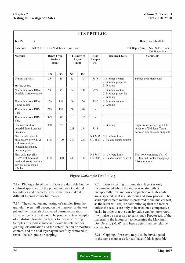
volume 7 section 3 part 2 Hd 29/08
t log date: 26 July 2006
Rut Depth (mm): Near Side = 3mm Off Side = 0mmtest mple no.
required tests comments
678 1. Bitumen content 2. Bitumen properties 3. Grading
Surface condition sound
679 1. Bitumen content 2. Bitumen properties 3. Grading
680 1. Bitumen content 2. Grading
-
-
681
1. Grading Slight water seepage @ 0.80m at centre of N/S lane. Terram between sub-base and subgrade
5682 5683
1. Atterberg limits 2. Field moisture content
5684 5685
1. Atterberg limits 2. Field moisture content
Trial hole terminated @ 1.30 - 1.40m with water seepage @ 0.80m as above
chapter 7 testing at investigation sites
test pitest pit: 17
location: M1 CH. 113 + 45 Northbound Slow Lane material depth from
surface (mm)
thickness of layer (mm)
sa
n/s o/s n/s o/s14mm slag HRA
Surface course
35 45 35 45 5
20mm limestone HRA Overlaid Surface course
99 95 64 50 5
28mm limestone HRA Binder course
159 151 60 56 5
40mm limestone DBM Base
219 191 60 40
40mm limestone DBM Base
329 306 110 115
Granular sub-base material Type 1 crushed limestone
850 870 521
564 5
Firm mottled grey & olive brown silty CLAY with traces of fine to medium sand and medium gravel
1100
1100
250
230
NSOS
Firm dark grey silty CLAY with traces of sand with some medium gravel size ironstone cobbles
1300
1400
200
300
NSOS
figure 7.2:samp
7.18 Photographs of the pit faces are desirable but the confined space within the pit and indistinct material boundaries and characteristics sometimes make it difficult to produce useful images.
7.19 The collection and testing of samples from the granular layers will depend on the purpose for the test pit and the materials discovered during excavation. However, generally it would be prudent to take samples of all distinct foundation layers for possible testing. Samples of sub-base material should be retained for grading, classification and the determination of moisture content, and the final layer again carefully removed to reveal the sub-grade or capping.
7/4
le test pit log
7.20 Density testing of foundation layers is only recommended where the stiffness or strength is unexpectedly low and low compaction or high voids are suspected, as it is a laborious and slow process. The sand replacement method is preferred to the nuclear test, as the latter will require calibration against the former unless the results are only to be used on a comparative basis. In order that the density value can be interpreted, it will also be necessary to carry out a Proctor test of the material in the laboratory to determine the Maximum Dry Density (MDD) and hence determine the relative compaction.
7.21 Capping, if present, may also be investigated in the same manner as for sub-base if this is possible
may 2008

volume 7 section 3 part 2 Hd 29/08
chapter 7 testing at investigation sites
in a safe manner. The record of the distribution of any moisture is particularly important. If the foundation layers in roads containing statutory undertakers equipment are holding water, samples may be taken for analysis, e.g. the presence of chlorine suggests that a water main may be leaking. Note must be made of any contamination between the subgrade and the sub-base or capping layers.
7.22 Samples of subgrade should be taken at 50mm depth and at 300mm depth for classification, including the determination of plastic limit, liquid limit and moisture content.
test pits in rigid pavements
7.23 The purposes for excavating test pits in rigid pavements are to investigate the following:
a) stepping/differential movement at joints;
b) very poor ‘load transfer’ at joints;
c) the possibility of suspect material beneath the concrete;
d) evidence of pumping at joints.
7.24 The reinstatement of concrete pavements after pitting is more difficult and disruptive than for asphalt materials. The new concrete will have to be left un-trafficked until a strength of 25N/mm2 is reached, thus increasing the delay and traffic disruption of the operation. Reinstatement with asphalt material must only be considered a temporary solution. For this reason, it is recommended that test pits should be made in concrete pavements only when it is considered absolutely necessary and no more than two joints are examined on any section. Consideration must be given to using large diameter (≥ 300mm) cores as an alternative to pitting.
may 2008
7.25 The recommended procedure is to saw cut the outline of the excavation, ensuring that it is taken far enough back from the joint to fully include the dowel bars (if any). Usually, only one side of the joint need be broken out, over a half lane width. Care must be taken when breaking out around dowel bars. The test pits, including any exposed dowels, should be photographed.
7.26 When replacing the concrete, it is essential that the joint is reformed, with intact dowel bars included, and the joint resealed (see HD 32 (DMRB 7.4.2)).
field tests on foundation materials
7.27 The Dynamic Cone Penetrometer (DCP) is recommended as the most suitable method for use in the bottom of core holes and test pits to indicate the strength and thickness of the foundation layers. The equipment is simple, fast and low cost. The essential features are shown in Figure 7.3.
7.28 The DCP uses an 8 Kg hammer dropping through a height of 575mm and a 60° cone having a maximum diameter of 20mm shown in Figure 1. The strength of the material is assessed on the rate of penetration per drop or “blow”. In practice the depth of penetration is recorded at increments of about 10mm, together with the number of blows to achieve this. The number of blows between readings will vary depending on the strength of the layer being penetrated.
7/5
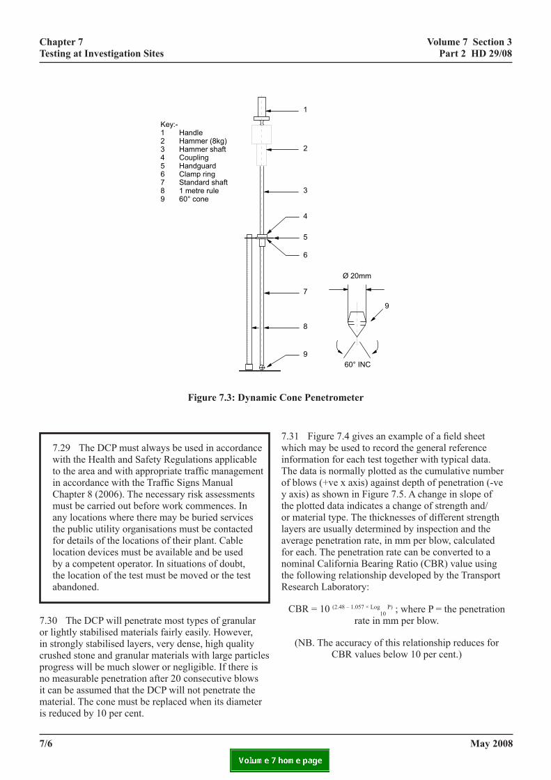
volume 7 section 3 part 2 Hd 29/08
one penetrometer
chapter 7 testing at investigation sites
C Volume 7 Section 3 T Part 2 HD 29/08
7
60° INC
Ø 20mm
7
8
9
5
4
9
1
2
3
6
one Penetrometer
7anblt
7spbb
7faidrd
figure 7.3: dynamic c
7.29 The DCP must always be used in accordance with the Health and Safety Regulations applicable to the area and with appropriate traffic management in accordance with the Traffic Signs Manual Chapter 8 (2006). The necessary risk assessments must be carried out before work commences. In any locations where there may be buried services the public utility organisations must be contacted for details of the locations of their plant. Cable location devices must be available and be used by a competent operator. In situations of doubt, the location of the test must be moved or the test abandoned.
7.30 The DCP will penetrate most types of granular or lightly stabilised materials fairly easily. However, in strongly stabilised layers, very dense, high quality crushed stone and granular materials with large particles progress will be much slower or negligible. If there is no measurable penetration after 20 consecutive blows it can be assumed that the DCP will not penetrate the material. The cone must be replaced when its diameter is reduced by 10 per cent.
7winToytholaafonthR
hapter 7 esting at Investigation Sites
·
Key:-1 Handle2 Hammer (8kg)3 Hammer shaft4 Coupling5 Handguard6 Clamp ring7 Standard shaft8 1 metre rule9 60° cone
Figure 7.3 Dynamic C
.29 The DCP must always be used in accordance with the nd with appropriate traffic management in accordance with ecessary risk assessments must be carried out before work curied services the public utility organisations must be contaocation devices must be available and be used by a competeest must be moved or the test abandoned.
.30 The DCP will penetrate most types of granular or lighttrongly stabilised layers, very dense, high quality crushed strogress will be much slower or negligible. If there is no meae assumed that the DCP will not penetrate the material. They 10 per cent.
.31 Figure 7.4 give an example of a field sheet which mayor each test together with typical data. The data is normallyxis) against depth of penetration (-ve y axis) as shown in Findicates a change of strength and/or material type. The thicketermined by inspection and the average penetration rate, inate can be converted to a nominal California Bearing Ratio (eveloped by the Transport Research Laboratory:
7/6
/6
CBR = 10 (2.48 – 1.057 × Log10
P) ; wher (NB. The accuracy of this relationship
.31 Figure 7.4 gives an example of a field sheet hich may be used to record the general reference formation for each test together with typical data. he data is normally plotted as the cumulative number f blows (+ve x axis) against depth of penetration (-ve axis) as shown in Figure 7.5. A change in slope of e plotted data indicates a change of strength and/
r material type. The thicknesses of different strength yers are usually determined by inspection and the
verage penetration rate, in mm per blow, calculated r each. The penetration rate can be converted to a
ominal California Bearing Ratio (CBR) value using e following relationship developed by the Transport esearch Laboratory:
CBR = 10 (2.48 – 1.057 × Log10
P) ; where P = the penetration rate in mm per blow.
(NB. The accuracy of this relationship reduces for CBR values below 10 per cent.)
Health and Safety Regulations applicable to the area the Traffic Signs Manual Chapter 8 (2006). The ommences. In any locations where there may be cted for details of the locations of their plant. Cable nt operator. In situations of doubt, the location of the
ly stabilised materials fairly easily. However, in one and granular materials with large particles surable penetration after 20 consecutive blows it can cone must be replaced when its diameter is reduced
be used to record the general reference information plotted as the cumulative number of blows (+ve x
gure 7.5. A change in slope of the plotted data nesses of different strength layers are usually mm per blow, calculated for each. The penetration CBR) value using the following relationship
may 2008
January 2008
e P = the penetration rate in mm per blow. reduces for CBR values below 10 per cent.)

volume 7 section 3 part 2 Hd 29/08
chapter 7 testing at investigation sites
dcp field sHeetProject: M1 J10/11 Job No: 45678 Operator: KG
Date: 4/6/06 Time: 22.30
Depth from road surface to start of test: 375mm
Notes: Drizzle
Test ID: C Lane: 1 Section: 50/8 Chainage: 31m Direction: NB Offset: 0.7m
No of blows
∑ blows
Penetration (mm)
No of blows
∑ blows
Penetration (mm)
No of blows
∑ blows
Penetration (mm)
0 0 393 2 21 593 2 69 742
1 1 431 2 23 605 2 71 751
1 2 451 2 25 611 2 73 765
1 3 466 2 27 614 1 74 778
1 4 475 4 31 621 1 75 805
1 5 486 4 35 627 1 76 840
1 6 496 4 39 635 1 77 850
1 7 504 4 43 642 1 78 863
1 8 511 4 47 650 1 79 870
1 9 516 4 51 665 1 80 878
2 11 525 4 55 676 1 81 888
2 13 534 4 59 694 1 82 906
2 15 545 4 63 710 1 83 920
2 17 561 2 65 721 1 84 935
2 19 581 2 67 732
figure 7.4: dynamic cone penetrometer field sheet example
may 2008 7/7
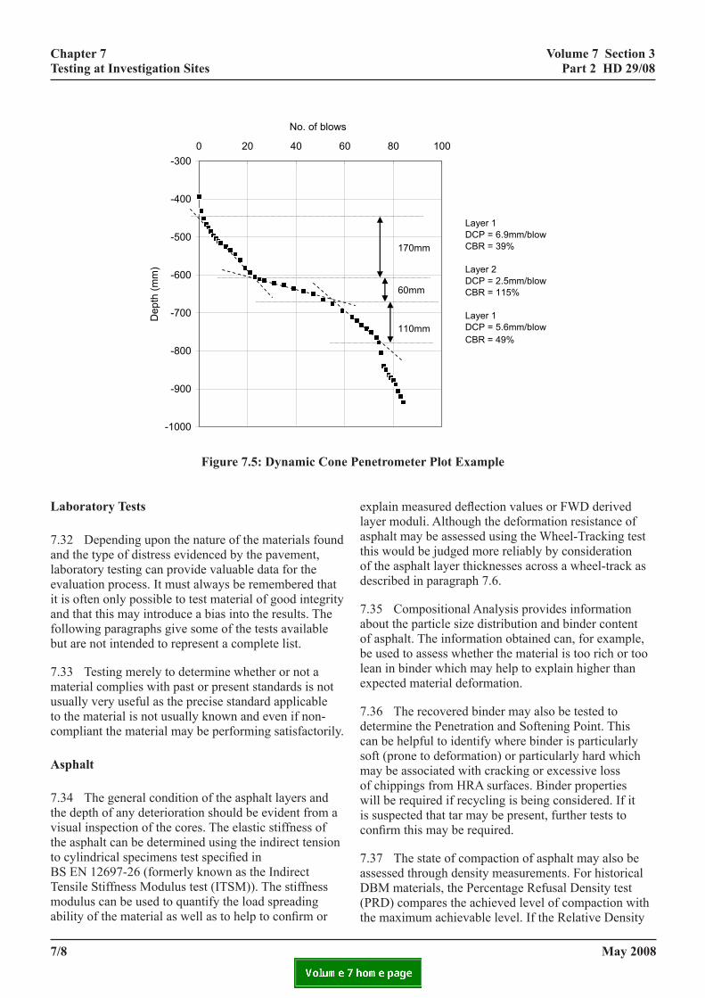
volume 7 section 3 part 2 Hd 29/08
chapter 7 testing at investigation sites
netrometer plot example
Chapter 7 Volume 7 Section 3 Testing at Investigation Sites Part 2 HD 29/08
80 100
Layer 1DCP = 6.9mm/blowCBR = 39%
Layer 2DCP = 2.5mm/blowCBR = 115%
Layer 1DCP = 5.6mm/blowCBR = 49%
170mm
60mm
110mm
figure 7.5: dynamic cone pelaboratory tests
7.32 Depending upon the nature of the materials found and the type of distress evidenced by the pavement, laboratory testing can provide valuable data for the evaluation process. It must always be remembered that it is often only possible to test material of good integrity and that this may introduce a bias into the results. The following paragraphs give some of the tests available but are not intended to represent a complete list.
7.33 Testing merely to determine whether or not a material complies with past or present standards is not usually very useful as the precise standard applicable to the material is not usually known and even if non-compliant the material may be performing satisfactorily.
asphalt
7.34 The general condition of the asphalt layers and the depth of any deterioration should be evident from a visual inspection of the cores. The elastic stiffness of the asphalt can be determined using the indirect tension to cylindrical specimens test specified in BS EN 12697-26 (formerly known as the Indirect Tensile Stiffness Modulus test (ITSM)). The stiffness modulus can be used to quantify the load spreading ability of the material as well as to help to confirm or
elatod
7aoble
7dcsmowic
7aD(t
7/8
-1000
-900
-800
-700
-600
-500
-400
-3000 20 40 60
No. of blows
Dep
th (m
m)
Figure 7.5 Dynamic Cone
Laboratory Tests
7.32 Depending upon the nature of the materials foundlaboratory testing can provide valuable data for the evaloften only possible to test material of good integrity andfollowing paragraphs give some of the tests available bu
7.33 Testing merely to determine whether or not a mavery useful as the precise standard applicable to the matmaterial may be performing satisfactorily.
Asphalt The general condition of the asphalt layers and the depthinspection of the cores. The elastic stiffness of the asphacylindrical specimens test specified in BS EN 12697-26test (ITSM)). The stiffness modulus can be used to quanhelp to confirm or explain measured deflection values oresistance of asphalt may be assessed using the Wheel-Tconsideration of the asphalt layer thicknesses across a w
7/8
xplain measured deflection values or FWD derived ayer moduli. Although the deformation resistance of sphalt may be assessed using the Wheel-Tracking test his would be judged more reliably by consideration f the asphalt layer thicknesses across a wheel-track as escribed in paragraph 7.6.
.35 Compositional Analysis provides information bout the particle size distribution and binder content f asphalt. The information obtained can, for example, e used to assess whether the material is too rich or too ean in binder which may help to explain higher than xpected material deformation.
.36 The recovered binder may also be tested to etermine the Penetration and Softening Point. This an be helpful to identify where binder is particularly oft (prone to deformation) or particularly hard which ay be associated with cracking or excessive loss
f chippings from HRA surfaces. Binder properties ill be required if recycling is being considered. If it
s suspected that tar may be present, further tests to onfirm this may be required.
.37 The state of compaction of asphalt may also be ssessed through density measurements. For historical BM materials, the Percentage Refusal Density test
PRD) compares the achieved level of compaction with he maximum achievable level. If the Relative Density
January 2008
Penetrometer Plot Example
and the type of distress evidenced by the pavement, uation process. It must always be remembered that it is that this may introduce a bias into the results. The t are not intended to represent a complete list.
terial complies with past or present standards is not usually erial is not usually known and even if non-compliant the
of any deterioration should be evident from a visual lt can be determined using the indirect tension to (formerly known as the Indirect Tensile Stiffness Modulus tify the load spreading ability of the material as well as to r FWD derived layer moduli. Although the deformation racking test this would be judged more reliably by heel-track as described in 7.5.
may 2008

volume 7 section 3 part 2 Hd 29/08
chapter 7 testing at investigation sites
of the mixture is measured together with the Bulk Density then volumetric proportions may be calculated including air void content.
Hydraulically Bound mixtures
7.38 The Cube Strength usually has to be deduced from cylinder tests. It also enables an estimate of flexural strength to be made, since direct testing in flexure is unlikely to be possible. The Density can be used to assess the degree of compaction achieved, particularly if an estimate of the Relative Density of the aggregate is available. As for asphalt, the Stiffness Modulus can be measured on either beam or cylindrical specimens, although it remains a specialist test.
unbound materials
7.39 Laboratory testing of the foundation layers, subbase or subgrade, should not normally be necessary as the DCP measurements should indicate the general condition and strength. However, tests may occasionally be necessary to explain the reasons for high or low strength or stiffness or to compare the material properties with specification standards. The most useful of these are:
• Grading;
• Liquid Limit, Plasticity Index and Linear Shrinkage;
• Moisture Content.
7.40 Where pavement failure is believed to be caused primarily by a weak foundation, a laboratory California Bearing Ratio (CBR) test of the material may be carried out, preferably by removing an undisturbed CBR mould-sized sample. (A disturbed CBR sample will also require an in situ density test to be carried out so that that the CBR material can be re-compacted to the in situ density.) An in situ CBR test is generally not very practical as it requires a large-plan test pit and takes considerable time, both of which add considerably to the cost.
may 2008 7/9

volume 7 section 3 part 2 Hd 29/08
ograpHY
chapter 8 references and Bibliography
8. references and BiBli
references
1. design manual for roads and Bridges (DMRB)
BA 86 (DMRB 3.1.7) Advice Notes on the Non-Destructive Testing of Highway Structures
HD 24 (DMRB 7.2.1) Traffic Assessment
HD 28 (DMRB 7.3.1) Skidding Resistance
HD 30 (DMRB 7.3.3) Maintenance Assessment Procedure
HD 31 (DMRB 7.4.1) Maintenance of Bituminous Roads
Traffic Appraisal Manual (DMRB 12.1)
2. transport research laboratory documents (TRL)
LR834; Kennedy, C.K., Fevre, P. and Clarke, C.S., Pavement deflection: equipment for measurement in the United Kingdom, TRRL
3. British standards
BS EN 12697-26:2004 Bituminous mixtures. Test methods for hot mix asphalt. Stiffness (2004)
4. statutory publications
Construction (Design and Management) Regulations (Northern Ireland), Statutory Rules of Northern Ireland, 2007 No. 291
Construction (Design and Management) Regulations, Statutory Instrument 2007 No. 320
Health and Safety at Work Act (1974)
Health and Safety at Work (Northern Ireland) Order 1979
Management of Health and Safety at Work Regulations (1999)
5.
Bi
may 2008
Management of Health and Safety at Work Regulations Statutory Rules of Northern Ireland, 2000 No 87
other publications
Network Management Manual, Version 1.5a, March 2007, Highways Agency
National Assembly for Wales Trunk Road Manual, National Assembly for Wales Transport Directorate
Concrete Pavement Maintenance Manual, 2001, Highways Agency and Britpave (published by the Concrete Society)
HAPMS Visual Survey Manual, Version 2.03, 2005, Highways Agency Pavement Management System
Scanner Surveys for Local Roads – User Guide and Specifications, 2007, UK Roads Board
bliography
LR833; Kennedy, C.K. and Lister, N.W., Prediction of Pavement Performance and the Design of Overlays, TRRL, 1978
LR1132; Powell, W.D., Potter, J.F., Mayhew, H.C. and Nunn, M.E., ‘The Structural Design of Bituminous Roads’, TRRL, 1984
Report 250; Nunn, M.E., Brown, A., Weston, D. and Nicholls, J.C., ‘Design of long-life flexible pavements for heavy traffic’, TRL, 1997
Daniels, D., Ground Penetrating Radar 2nd Edition (Radar, Sonar, Navigations & Avionics), 2004, The Institution of Electrical Engineers, London. (ISBN 0 86341 360 9)
Hopman, V. and Beuving, E., Repeatability, reproducibility and accuracy of GPR measurements. Bearing Capacity of Roads, Railways and Airfields, Correia & Branco (eds), 2002 (ISBN 905809 396 4)
8/1

may 2008
volume 7 section 3 part 2 Hd 29/08
9. enQuiries
All technical enquiries or comments on this Standard should be sent in writing as appropriate to:
Chief Highway Engineer The Highways Agency 123 Buckingham Palace Road London G CLARKE SW1W 9HA Chief Highway Engineer
Director, Major Transport Infrastructure Projects Transport Scotland 8th Floor, Buchanan House 58 Port Dundas Road A C McLAUGHLIN Glasgow Director, Major Transport Infrastructure G4 0HF Projects
Chief Highway Engineer Transport Wales Welsh Assembly Government Cathays Parks M J A PARKER Cardiff Chief Highway Engineer CF10 3NQ Transport Wales
Director of Engineering The Department for Regional Development Roads Service Clarence Court 10-18 Adelaide Street R J M CAIRNS Belfast BT2 8GB Director of Engineering
9/1
chapter 9 enquiries

may 2008
volume 7 section 3 part 2 Hd 29/08
annex 1 not currentlY used
a1/1
annex 1
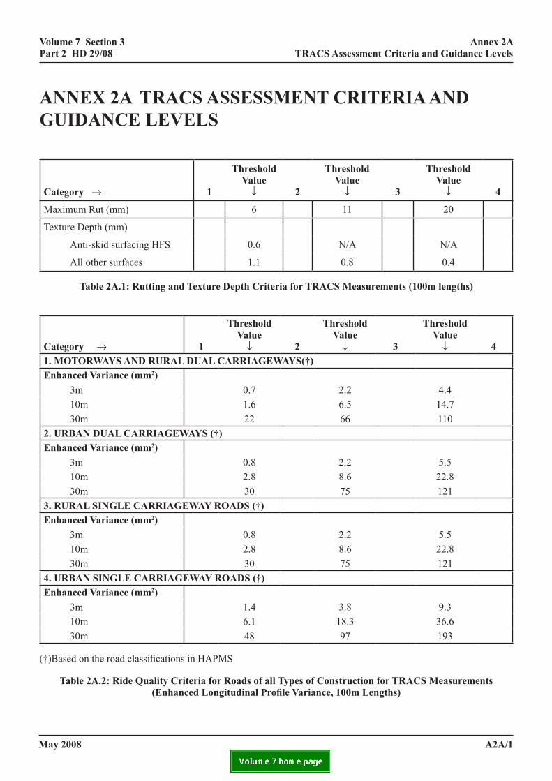
may 2008
volume 7 section 3 part 2 Hd 29/08
annex 2a tracs assessment criteria and guidance levels
category →
1
threshold value
↓
2
threshold value
↓
3
threshold value
↓
4
Maximum Rut (mm) 6 11 20
Texture Depth (mm)
Anti-skid surfacing HFS 0.6 N/A N/A
All other surfaces 1.1 0.8 0.4
Table 2A.1: Rutting and Texture Depth Criteria for TRACS Measurements (100m lengths)
category →
1
threshold value
↓
2
threshold value
↓
3
threshold value
↓
4
1. MOTORWAYS AND RURAL DUAL CARRIAgEWAYS(†)Enhanced Variance (mm2) 3m 0.7 2.2 4.4 10m 1.6 6.5 14.7 30m 22 66 1102. URBAN DUAL CARRIAgEWAYS (†)Enhanced Variance (mm2) 3m 0.8 2.2 5.5 10m 2.8 8.6 22.8 30m 30 75 1213. RURAL SINgLE CARRIAgEWAY ROADS (†)Enhanced Variance (mm2) 3m 0.8 2.2 5.5 10m 2.8 8.6 22.8 30m 30 75 1214. URBAN SINgLE CARRIAgEWAY ROADS (†)Enhanced Variance (mm2) 3m 1.4 3.8 9.3 10m 6.1 18.3 36.6 30m 48 97 193
(†)Based on the road classifications in HAPMS
table 2a.2: ride Quality criteria for roads of all types of construction for tracs measurements (Enhanced Longitudinal Profile Variance, 100m Lengths)
a2a/1
annex 2a tracs assessment criteria and guidance levels

may 2008
volume 7 section 3 part 2 Hd 29/08
category →
Low
threshold Value (%)
↓
moderate
threshold Value (%)
↓
High
Asphalt Surface – Hot Rolled Asphalt Thresholds for cracking have yet to be decided for the new TRACS contractor. These will be made available once further research has
been completed.Asphalt Surface – Other
Concrete Surface
Table 2A.3: guidance Levels for TRACS Whole Carriageway Cracking Intensities (100m Lengths) (Refer also to Annex 2B when Assessing the Cracking Data)
category →
Low
threshold Value (%)
↓
moderate
threshold Value (%)
↓
High
threshold Value (%)
↓
severeAsphalt Surface – Hot Rolled Asphalt
0.20 1.15 1.80
Bituminous Surface – Other N/A N/A N/A
Table 2A.4: guidance Levels for Fretting (100m Lengths)
a2a/2
annex 2a tracs assessment criteria and guidance levels
volume 7 section 3 part 2 Hd 29/08
ription of tracs
annex 2B detailed description of tracs condition data
annex 2B detailed desccondition data
texture depth
2B.1 The surface Texture Depth measured by the TRACS survey vehicle is the coarser element of macrotexture and the finer element of megatexture formed by aggregate particles in the asphalt surfacing or by the brushing or grooving of concrete surfacing. Texture Depth contributes to skidding resistance, primarily at medium and high speeds, in two ways. Firstly, it provides drainage paths to allow water to be removed rapidly from the tyre/road interface. Secondly, the projections, which contribute to hysteresis losses in the tyre, are an important factor in the braking process.
2B.2 The Machine Survey Pre-processor (MSP) software calculates Sensor Measured Texture Depth (SMTD) from the raw Texture Profile measurements collected by the TRACS survey vehicle for the near side wheel-track and averages them over 10m lengths for storage as Base Data within HAPMS.
rut depth
2B.3 To measure Rut Depth, the TRACS survey vehicle records the Transverse Profile of the road surface over a width of 3.2m using 20 laser sensors. The Transverse Profile measurements are processed in MSP, which uses an algorithm to simulate placing a notional 2m straight edge on the recorded Transverse Profile, and measuring the largest deviation from the straight edge to the Transverse Profile. This calculation is carried out for each wheel-track. MSP calculates the average of the individual Rut Depths for each wheel-track over 10m lengths for storage within HAPMS.
2B.4 The Transverse Profile measurement method of Rut Depth determination used by the TRACS vehicle has been shown to be highly comparable with the measurements made using a conventional straight edge and wedge.
2B.5 TRACS Rut Depth measurements can sometimes be affected by variations in driving line. When the survey vehicle drives to the nearside of the traffic lane the lane edge marking may be included in the Transverse Profile measurement, giving rise to nearside Rut Depths that are higher than those actually
may 2008
present on the pavement. Similarly, driving to the offside can result in lower nearside Rut Depths.
2B.6 It is recommended that, where any length has been identified for further investigation as a result of deep Rut Depths, that comparison be made between the Left Rut and Right Rut length weighted average values contained within HAPMS. This is to check that there are no excessive differences which could be caused by the inclusion of the edge line in the Left Rut measurements.
ride Quality
2B.7 The parameter currently used for the assessment of Ride Quality, or Profile Unevenness, is the Enhanced Longitudinal Profile Variance of individual deviations of the profile relative to a datum obtained by removing (or filtering) longer wavelengths from the measured longitudinal profile. This parameter was introduced in June 2004 and uses sophisticated filtering which removes the effects of the pavement geometry (gradient, crossfall and curvature), which had previously caused high levels of variance at, for example, the approaches to roundabouts. The previous simpler method of filtering produced the parameter Longitudinal Profile Variance.
2B.8 The Enhanced Longitudinal Profile Variance value reflects the unevenness associated with profile features that are equal to or less in wavelength than the length of the filter used to calculate the Enhanced Longitudinal Profile Variance. For example, the variance of deviations from a 3m filter reflects the unevenness of profile features with wavelengths equal to or less than approximately 3m.
2B.9 The measurement of Profile Unevenness can be used to investigate the Ride Quality of the pavement. The short, medium and long wavelength features are found to relate with the perceived effect on vehicle ride are represented by variance from 3m, 10m and 30m filters respectively. The 3m, 10m and 30m Enhanced Longitudinal Profile Variance values are calculated from the TRACS longitudinal profile measurements by MSP and averaged over 10m lengths for storage within HAPMS.
a2B/1
volume 7 section 3 part 2 Hd 29/08
annex 2B detailed description of tracs condition data
2B.10 Extremes of 10m Enhanced Longitudinal Profile Variance may arise from poor reinstatements along the wheel-track, the presence of high and/or variable levels of rutting, and bay length irregularities (in concrete roads). High levels of 30m Enhanced Longitudinal Profile Variance may be associated with subsidence. Changes of crossfall along the length of a road may also result in slightly higher 30m ELPV being reported.
2B.11 High levels of Profile Unevenness do not only affect Ride Quality. High levels of Profile Unevenness, particularly in the 3m and 10m wavelength ranges, have been shown to contribute to increased dynamic loading of the pavement, hence accelerating the deterioration of the road pavement. Extremes of Profile Unevenness can also lead to increased stopping distances, and can have an adverse effect on vehicle manoeuvrability and safety.
2B.12 The values of Enhanced Longitudinal Profile Variance calculated from TRACS Longitudinal Profile measurements must not be compared directly with either values of Moving Average Longitudinal Profile Variance (produced by TRACS surveys prior to 1st June 2004) or, the values of Moving Average Longitudinal Profile Variance provided by earlier HRM surveys. This is because there are significant differences in the scaling of the data and the Enhanced Longitudinal Profile Variance measure generally reports lower values than the other two systems. However, the Moving Average Longitudinal Profile Variance and Enhanced Longitudinal Profile Variance methods are well correlated. On lengths where there is little variation in the geometry they will, in general, agree with regard to the locations at which higher values are reported. On lengths containing variations in the geometry the Enhanced Longitudinal Profile Variance is likely to report lower values.
a2B/2
2B.13 Further research carried out on TRACS measurements has shown that the TRACS survey vehicle may provide Longitudinal Profile data having lower levels of accuracy when surveying at slow speed, or under conditions of significant acceleration or (more commonly) deceleration. To reduce the occurrence of low accuracy data, limits have been specified for the TRACS surveys for speed and acceleration/deceleration beyond which the data is considered invalid. Where these limits have been exceeded the data is marked as Unreliable in the TRACS Base LPV Data. The presence of a significant proportion of Unreliable values within any 100m length will result in missing values when the data is expressed as 100m Length Weighted Averages in HAPMS.
2B.14 Ride Quality measurements provided by TRACS surveys prior to 1st June 2004 were reported as Moving Average Longitudinal Profile Variance. As the TRACS Length Weighted Averages data source in HAPMS reports the most recent TRACS data, the data source may contain data collected prior to 1st June 2004.
2B.15 To distinguish between Moving Average LPV and Enhanced LPV, the TRACS Length Weighted Averages data source in HAPMS provides an additional label for the LPV data called “Enhanced”. Where the label is not present this indicates that the value reported in the HAPMS TRACS Length Weighted Averages data source is the old Moving Average Longitudinal Profile Variance.
2B.16 Where it is required that an assessment be made of TRACS measurements of Moving Average Longitudinal Profile Variance (for TRACS surveys carried out before 1 June 2004) it will be necessary to apply the thresholds given in Table 2B.1.
may 2008
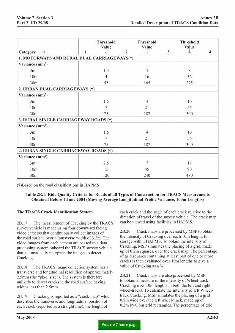
volume 7 section 3 part 2 Hd 29/08
2
threshold value
↓
3
threshold value
↓
4
YS(†)
4 816 36165 275
4 1021 56187 300
4 1021 56187 300
7 1745 90
annex 2B detailed description of tracs condition data
category →
1
threshold value
↓1. MOTORWAYS AND RURAL DUAL CARRIAgEWAVariance (mm2) 3m 1.3 10m 4 30m 552. URBAN DUAL CARRIAgEWAYS (†)Variance (mm2) 3m 1.5 10m 7 30m 753. RURAL SINgLE CARRIAgEWAY ROADS (†)Variance (mm2) 3m 1.5 10m 7 30m 754. URBAN SINgLE CARRIAgEWAY ROADS (†)Variance (mm2) 3m 2.5 10m 15 30m 120
(†)Based on the road classifications in HAPMS
table 2B.1: ride Quality criteria for roads of all tyObtained Before 1 June 2004 (Moving Average L
The TRACS Crack Identification System
2B.17 The measurement of Cracking by the TRACS survey vehicle is made using four downward facing video cameras that continuously collect images of the road surface over a transverse width of 3.2m. The video images from each camera are passed to a data processing system onboard the TRACS survey vehicle that automatically interprets the images to detect Cracking.
2B.18 The TRACS image collection system has a transverse and longitudinal resolution of approximately 2.5mm (the “pixel size”). The system is therefore unlikely to detect cracks in the road surface having widths less than 2.5mm.
2B.19 Cracking is reported as a “crack map” which describes the transverse and longitudinal position of each crack (reported as a straight line), the length of
edc
2thstCuocv
2toCwtr00
may 2008
240 480
pes of construction for tracs measurements ongitudinal Profile Variance, 100m Lengths)
ach crack and the angle of each crack relative to the irection of travel of the survey vehicle. The crack map an be viewed using facilities in HAPMS.
B.20 Crack maps are processed by MSP to obtain e intensity of Cracking over each 10m length, for orage within HAPMS. To obtain the intensity of racking, MSP simulates the placing of a grid, made p of 0.2m squares, over the crack map. The percentage f grid squares containing at least part of one or more racks is then evaluated over 10m lengths to give a alue of Cracking as a %.
B.21 Crack maps are also processed by MSP obtain a measure of the intensity of Wheel-track racking over 10m lengths in both the left and right heel-tracks. To calculate the intensity of left Wheel-ack Cracking, MSP simulates the placing of a grid .8m wide over the left wheel-track, made up of .2m by 0.8m grid rectangles. The percentage of grid
a2B/3
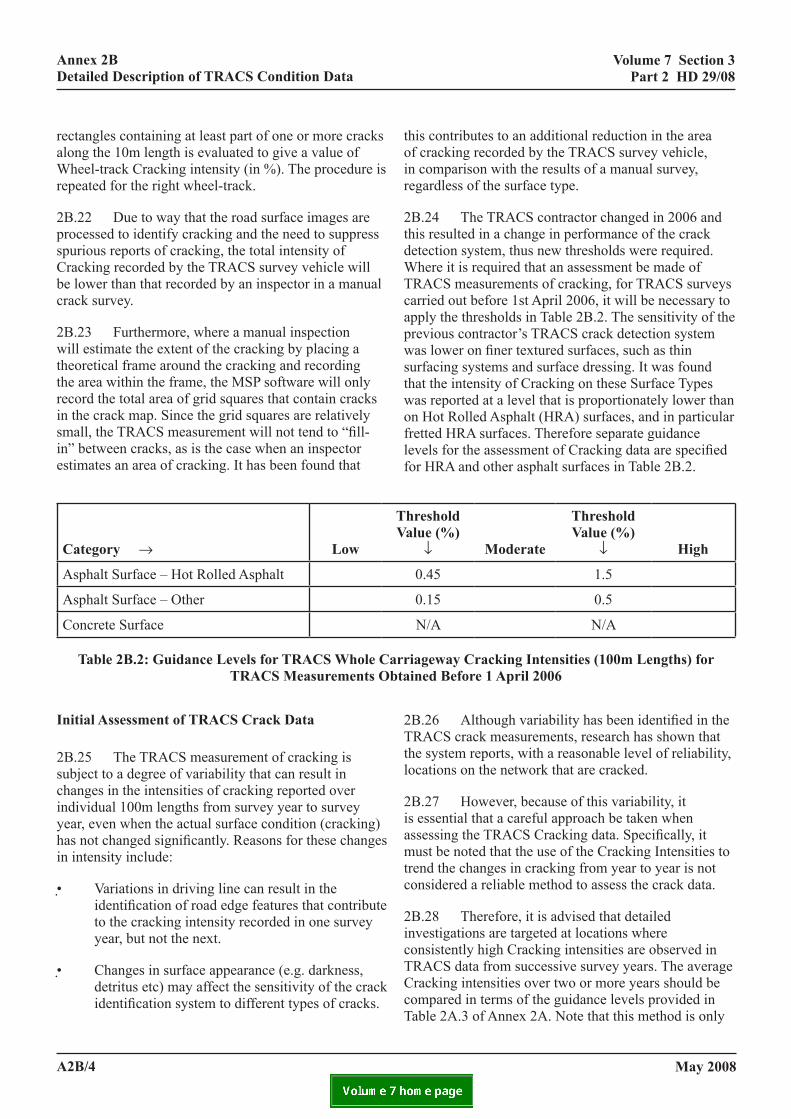
volume 7 section 3 part 2 Hd 29/08
annex 2B detailed description of tracs condition data
rectangles containing at least part of one or more cracks along the 10m length is evaluated to give a value of Wheel-track Cracking intensity (in %). The procedure is repeated for the right wheel-track.
2B.22 Due to way that the road surface images are processed to identify cracking and the need to suppress spurious reports of cracking, the total intensity of Cracking recorded by the TRACS survey vehicle will be lower than that recorded by an inspector in a manual crack survey.
2B.23 Furthermore, where a manual inspection will estimate the extent of the cracking by placing a theoretical frame around the cracking and recording the area within the frame, the MSP software will only record the total area of grid squares that contain cracks in the crack map. Since the grid squares are relatively small, the TRACS measurement will not tend to “fill-in” between cracks, as is the case when an inspector estimates an area of cracking. It has been found that
category →
Low
tV
Asphalt Surface – Hot Rolled Asphalt
Asphalt Surface – Other
Concrete Surface
Table 2B.2: guidance Levels for TRACS Whole Cartracs measurements obta
initial assessment of tracs crack data
2B.25 The TRACS measurement of cracking is subject to a degree of variability that can result in changes in the intensities of cracking reported over individual 100m lengths from survey year to survey year, even when the actual surface condition (cracking) has not changed significantly. Reasons for these changes in intensity include:
• Variations in driving line can result in the identification of road edge features that contribute to the cracking intensity recorded in one survey year, but not the next.
• Changes in surface appearance (e.g. darkness, detritus etc) may affect the sensitivity of the crack identification system to different types of cracks.
a2B/4
this contributes to an additional reduction in the area of cracking recorded by the TRACS survey vehicle, in comparison with the results of a manual survey, regardless of the surface type.
2B.24 The TRACS contractor changed in 2006 and this resulted in a change in performance of the crack detection system, thus new thresholds were required. Where it is required that an assessment be made of TRACS measurements of cracking, for TRACS surveys carried out before 1st April 2006, it will be necessary to apply the thresholds in Table 2B.2. The sensitivity of the previous contractor’s TRACS crack detection system was lower on finer textured surfaces, such as thin surfacing systems and surface dressing. It was found that the intensity of Cracking on these Surface Types was reported at a level that is proportionately lower than on Hot Rolled Asphalt (HRA) surfaces, and in particular fretted HRA surfaces. Therefore separate guidance levels for the assessment of Cracking data are specified for HRA and other asphalt surfaces in Table 2B.2.
hreshold alue (%)
↓
moderate
threshold Value (%)
↓
High
0.45 1.5
0.15 0.5
N/A N/A
riageway Cracking Intensities (100m Lengths) for ined Before 1 april 2006
2B.26 Although variability has been identified in the TRACS crack measurements, research has shown that the system reports, with a reasonable level of reliability, locations on the network that are cracked.
2B.27 However, because of this variability, it is essential that a careful approach be taken when assessing the TRACS Cracking data. Specifically, it must be noted that the use of the Cracking Intensities to trend the changes in cracking from year to year is not considered a reliable method to assess the crack data.
2B.28 Therefore, it is advised that detailed investigations are targeted at locations where consistently high Cracking intensities are observed in TRACS data from successive survey years. The average Cracking intensities over two or more years should be compared in terms of the guidance levels provided in Table 2A.3 of Annex 2A. Note that this method is only
may 2008
volume 7 section 3 part 2 Hd 29/08
annex 2B detailed description of tracs condition data
applicable for lengths where no maintenance has been carried out during the averaging period.
2B.29 This approach must enable more reliable identification of lengths with high levels of cracking present. Further investigation of these lengths must begin with the examination of the crack map data contained in HAPMS. This must be carried out using the most recent survey year and, where available, at least two preceding survey years.
fretting
2B.30 On pavements having coarse textures with large chip size, such as Hot Rolled Asphalt (HRA), the presence of severe Fretting (loss of stone from the surface) may be reported as Cracking by the TRACS survey vehicle. This can lead to lengths reported as containing high levels of Cracking that, in a visual survey, may have been reported as containing high levels of minor deterioration. TRACS surveys only measure fretting in the near side wheel-track.
2B.31 An estimate of the extent of Fretting can be derived from the Texture Profile by identifying characteristic shapes resulting from missing surface aggregate. Algorithms have been developed on this basis and incorporated into the MSP software to provide an indication of the presence of Fretting.
2B.32 The Fretting algorithms are currently optimised for the identification of Fretting of HRA. On other Surface Types the algorithms will generally report levels close to zero. Therefore, the Fretting data reported in HAPMS must only be used in the assessment of HRA surfaces.
2B.33 The Fretting algorithm reports the intensity of Fretting as a percentage value. The guidance levels for the assessment of Fretting have been obtained by undertaking manual surveys of fretted HRA pavements and comparing the reported levels of Fretting with those reported by the Fretting algorithm. It can be seen that the threshold levels have reasonably low absolute values. This is a result of the Fretting calculation process and its relationship to the identification of missing aggregate particles. The values must not be compared directly with measures obtained from manual visual condition surveys.
2utCha
2p
may 2008
B.34 The Fretting data is, in particular, intended for se when assessing the condition of HRA pavements hat have been reported to contain high levels of racking. Where both the Fretting and Cracking report igh levels it is probable that the crack measurements re actually reporting the presence of Fretting.
B.35 The crack map may be also used to show the resence of Fretting in the crack data.
a2B/5

may 2008
volume 7 section 3 part 2 Hd 29/08
annex 3 currentlY not used
a3/1
annex 3
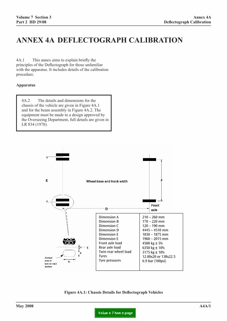
volume 7 section 3 part 2 Hd 29/08
annex 4a Deflectograph Calibration
annex 4a deflectograpH caliBration
4A.1 This annex aims to explain briefly the principles of the Deflectograph for those unfamiliar with the apparatus. It includes details of the calibration procedure.
apparatus
4A.2 The details and dimensions for the chassis of the vehicle are given in Figure 4A.1 and for the beam assembly in Figure 4A.2. The equipment must be made to a design approved by the Overseeing Department, full details are given in LR 834 (1978).
Figure 4A.1: Chassis Details for Deflectograph Vehicles
Volume 7 Section 3 Annex 4APart 2 HD 29/08 Deflectograph Calibration
ANNEX 4A – DEFLECTOGRAPH CALIBRATION 4A.1 This annex aims to explain briefly the principles of the Deflectograph for those unfamiliar with the apparatus. It includes details of the calibration procedure.
Apparatus
4A.2 The details and dimensions for the chassis of the vehicle are given in Figure 4A.1 and for the beam assembly in Figure 4A.2. The equipment must be made to a design approved by the Overseeing Department, full details are given in LR 834 (1978).
Figure 4A.1 Chassis Details for Deflectograph Vehicles
Dimension A Dimension B Dimension C Dimension D Dimension E Dimension E Front axle load Rear axle load Twin rear wheel load Tyres Tyre pressures
210 – 260 mm 170 – 220 mm 120 – 190 mm 4445 – 4510 mm 1830 – 1875 mm 1960 – 2015 mm 4500 kg ± 5% 6350 kg ± 10% 3175 kg ± 10% 12.00x20 or 13Rx22.5 6.9 bar (100psi)
may 2008 a4a/1
January 2008 A4A/1
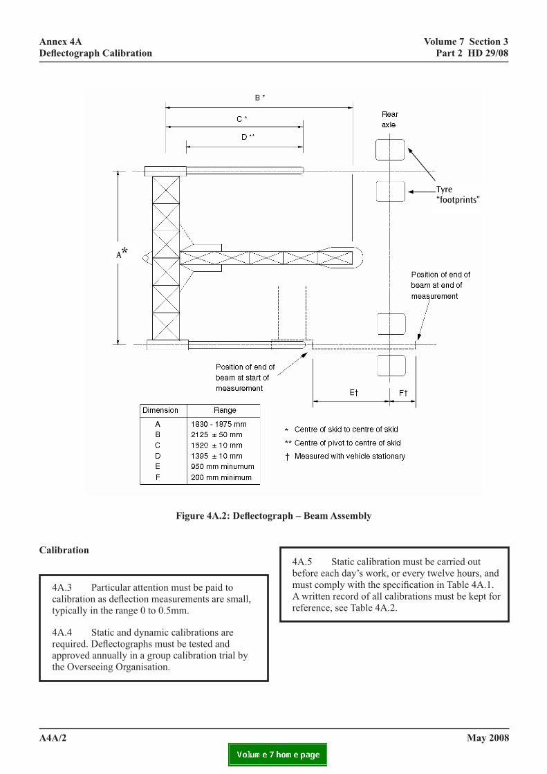
volume 7 section 3 part 2 Hd 29/08
c
a
annex 4a Deflectograph CalibrationAnnex 4A Volume 7 Section 3
Deflectograph Calibration Part 2 HD 29/08
each day's work, or every twelve hours, and must comply rd of all calibrations must be kept for reference, see Table
Tyre “footprints”
Figure 4A.2: Deflecto
alibration
4A.3 Particular attention must be paid to calibration as deflection measurements are small, typically in the range 0 to 0.5mm.
4A.4 Static and dynamic calibrations are required. Deflectographs must be tested and approved annually in a group calibration trial by the Overseeing Organisation.
FIGURE 4A.2 Defle
Calibration
4A.3 Particular attention must be paid to calibratiorange 0 to 0.5mm.
4A.4 Static and dynamic calibrations are required.group calibration trial by the Overseeing Organisat
4A.5 Static calibration must be carried out before with the specification in Table 4A.1. A written reco
A*
4a/2A4A/2
4A.2.
graph – Beam Assembly
4A.5 Static calibration must be carried out before each day’s work, or every twelve hours, and must comply with the specification in Table 4A.1. A written record of all calibrations must be kept for reference, see Table 4A.2.
ctograph - Beam Assembly
n as deflection measurements are small, typically in the
Deflectographs must be tested and approved annually in a ion.
may 2008January 2008
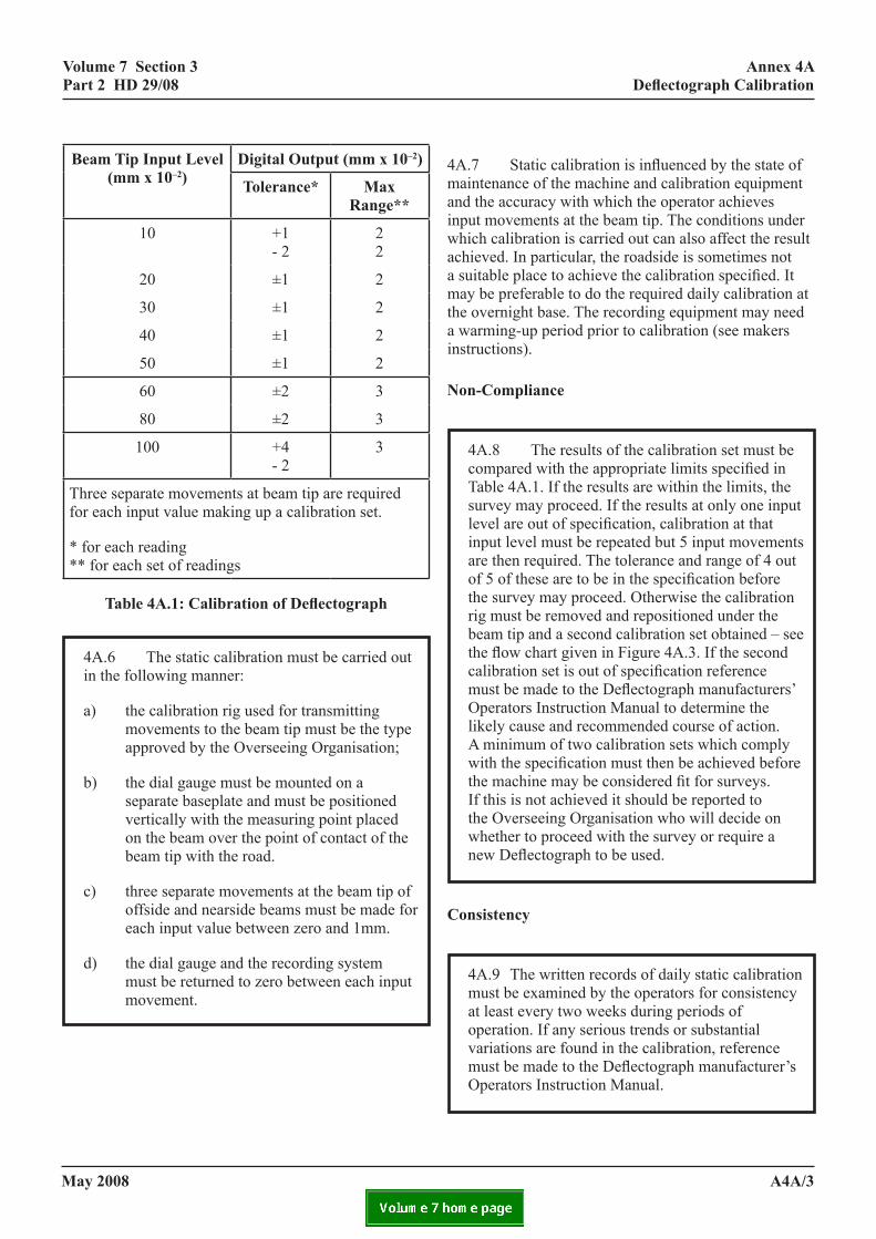
volume 7 section 3 part 2 Hd 29/08
annex 4a Deflectograph Calibration
Beam tip input level (mm x 10–2)
Digital Output (mm x 10–2)
tolerance* max range**
10 +1 - 2
2 2
20 ±1 2
30 ±1 2
40 ±1 2
50 ±1 2
60 ±2 3
80 ±2 3
100 +4 - 2
3
Three separate movements at beam tip are required for each input value making up a calibration set.
* for each reading ** for each set of readings
Table 4A.1: Calibration of Deflectograph
4A.6 The static calibration must be carried out in the following manner:
a) the calibration rig used for transmitting movements to the beam tip must be the type approved by the Overseeing Organisation;
b) the dial gauge must be mounted on a separate baseplate and must be positioned vertically with the measuring point placed on the beam over the point of contact of the beam tip with the road.
c) three separate movements at the beam tip of offside and nearside beams must be made for each input value between zero and 1mm.
d) the dial gauge and the recording system must be returned to zero between each input movement.
may 2008
4A.7 Static calibration is influenced by the state of maintenance of the machine and calibration equipment and the accuracy with which the operator achieves input movements at the beam tip. The conditions under which calibration is carried out can also affect the result achieved. In particular, the roadside is sometimes not a suitable place to achieve the calibration specified. It may be preferable to do the required daily calibration at the overnight base. The recording equipment may need a warming-up period prior to calibration (see makers instructions).
Non-Compliance
4A.8 The results of the calibration set must be compared with the appropriate limits specified in Table 4A.1. If the results are within the limits, the survey may proceed. If the results at only one input level are out of specification, calibration at that input level must be repeated but 5 input movements are then required. The tolerance and range of 4 out of 5 of these are to be in the specification before the survey may proceed. Otherwise the calibration rig must be removed and repositioned under the beam tip and a second calibration set obtained – see the flow chart given in Figure 4A.3. If the second calibration set is out of specification reference must be made to the Deflectograph manufacturers’ Operators Instruction Manual to determine the likely cause and recommended course of action. A minimum of two calibration sets which comply with the specification must then be achieved before the machine may be considered fit for surveys. If this is not achieved it should be reported to the Overseeing Organisation who will decide on whether to proceed with the survey or require a new Deflectograph to be used.
consistency
4A.9 The written records of daily static calibration must be examined by the operators for consistency at least every two weeks during periods of operation. If any serious trends or substantial variations are found in the calibration, reference must be made to the Deflectograph manufacturer’s Operators Instruction Manual.
a4a/3

volume 7 section 3 part 2 Hd 29/08
Date:
Number:
(of calibration)
n Mean Calibration
◊
N/S O/S
ecord
annex 4a Deflectograph Calibration
DEFLECTOGRAPH STATIC CALIBRATION
Purpose: SURVEY/MACHINE CHECK*
Location: BASE/ROADSIDE*
Beam Tip Input
(mm x 10-2)
Digital Output
Compliance with Specificaito
Nearside Offside N/S O/S
10
20
30
40
50
60
80
100
* Delete as necessary ◊ Values for calibration correction program should be to one decimal place
Table 4A.2: Deflectograph Static Calibration R
calibration correction by computer program
4A.10 The calibrations to be entered must be the mean of the results of all calibration sets taken on the day of the survey that comply with the Specification.
servicing of calibration equipment
4A.11 The calibration rig must be kept in good condition. The dial gauge must be serviced and checked against a standard gauge at least annually.
may 2008a4a/4
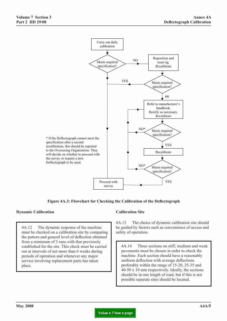
volume 7 section 3 part 2 Hd 29/08
annex 4a Deflectograph Calibration
Annex 4A Volume 7 Section 3 Deflectograph Calibration Part 2 HD 29/08
rn e. er
safety
ach 5-20,
Reposition and reset rig.
Recalibrate
Meets required specification?
Refer to manufacturer’s handbook.
Rectify as necessary. Recalibrate
Recalibrate
Meets required specification?
Meets required specification?
NO
NO*
NO
YES
NO*
YES
Figure 4A.3: Flowchart for Checking the
dynamic calibration
4A.12 The dynamic response of the machine must be checked on a calibration site by comparing the pattern and general level of deflection obtained from a minimum of 3 runs with that previously established for the site. This check must be carried out at intervals of not more than 6 weeks during periods of operation and whenever any major service involving replacement parts has taken place.
c
4Abesa
FIGURE 4A.3 Flowchart for
Dynamic Calibration
4A.12 The dynamic response of the machine and general level of deflection obtained from a mThis check must be carried out at intervals of noany major service involving replacement parts h
Calibration Site
4A.13 The choice of dynamic calibration site shoof operation.
4A.14 Three sections on stiff, medium and weaksection should have a reasonably uniform deflec25-35 and 40-50 x 10 mm respectively. Ideally,possible separate sites should be located.
Carry out daily calibration
Proceed with survey
Meets required specification?
* If the Deflectograph cannot meet the specification after a second recalibration, this should be reported to the Overseeing Organisation. They will decide on whether to proceed with the survey or require a new Deflectograph to be used.
may 2008 A4A/6
4A.15 On each section there should be s
Calibration of the Deflectograph
alibration site
.13 The choice of dynamic calibration site should guided by factors such as convenience of access and fety of operation.
4A.14 Three sections on stiff, medium and weak pavements must be chosen in order to check the machine. Each section should have a reasonably uniform deflection with average deflections preferably within the range of 15-20, 25-35 and 40-50 x 10 mm respectively. Ideally, the sections should be in one length of road, but if this is not possible separate sites should be located.
Checking the Calibration of the Deflectograph
must be checked on a calibration site by comparing the patteinimum of 3 runs with that previously established for the sit
t more than 6 weeks during periods of operation and whenevas taken place.
uld be guided by factors such as convenience of access and
pavements must be chosen in order to check the machine. Etion with average deflections preferably within the range of 1 the sections should be in one length of road, but if this is not
ufficient reference points to ensure accurate location of deflections.
YES
a4a/5January 2008
volume 7 section 3 part 2 Hd 29/08
annex 4a Deflectograph Calibration
4A.15 On each section there should be sufficient reference points to ensure accurate location of deflections.
4A.16 The sections should not be too heavily trafficked, thus giving a long useful life as calibration lengths and obviating the need for frequent updating of the deflections to allow for traffic carried. A recently by-passed section of road would appear appropriate.
4A.17 The drainage should be satisfactory so as to keep the seasonal variation of results to a minimum.
4A.18 Each section should have a uniform road surface and not be subject to sun/shadow effect making it difficult to determine pavement temperatures accurately.
4A.19 If the pavement contains hydraulically bound material it should be uncracked otherwise the deflection profile is liable to be excessively variable.
4A.20 The surface course of any type of pavement should be in sound, uncracked condition, preferably with wheel-track rutting less than 5 mm deep. This requirement may be difficult to attain where a pavement in the highest deflection range is required and a lesser standard may have to be accepted. However, rut depths of 10 mm should be considered the absolute maximum.
4A.21 The gradient of the road should not exceed 4 per cent. A steeper gradient could have an adverse effect when checking the machine by measuring the same wheel-tracks in different directions.
4A.22 The deflection profile of the test sections at the calibration site should be established for a range of temperatures using a Deflectograph of known satisfactory performance. This will involve making at least five runs with the machine on each of several occasions during the year when suitable temperatures occur. For each wheel-track the overall mean deflection of each section and the variability should be calculated for each temperature at which measurements are taken.
procedure
4A.23 At least one calibration set must precede and follow the dynamic calibration, which comprises a minimum of 3 runs over the test sections of the calibration site.
a
f
4Aarininita iswofde31toprTenan
4Avebewdeth
a4a/6
ssessment of results
4A.24 Results of the calibration runs must be compared with those already established for the site at the temperature of the test. It should be remembered that measurements with a Deflectograph may be taken at slightly different locations on each run, therefore the mean deflection values for different runs are not from identical samples. However, if there are any major discrepancies between the results these must be investigated by checking that there have not been any changes in conditions at the calibration site or in factors affecting the dynamic response of the machine. If an imbalance between nearside and offside results is suspected, further runs in which the nearside beam follows the track previously measured by the offside beam must be made. (This may be achieved by testing the site in the reverse direction).
actors affecting dynamic response of machine
.25 The permitted weights given in Figure 4A.1 e for the vehicle plus crew with the beam assembly the carrying position. The load on the front wheels fluences the magnitude of the measured deflection. As is not possible to use a simple scaling factor to apply correction, it is most important that the front axle load as close as possible to the value specified. If the rear heel loading is different from the recommended value 3175 kg, but within the tolerance allowed, measured flections must be multiplied by a correction factor of 75/(actual wheel loading). This correction is made all measured deflections by the PANDEF computer ogram when actual rear wheel weights are entered. he intention is that typical average values should be tered, as weights will vary depending on fuel carried d the number of crew on board.
.26 The position of the T frame relative to the hicle axles is important because the front skids can within the deflection bowl generated by the front heels of the machine. The shape of this bowl varies pending on the type of pavement material used and e magnitude of the deflection.
may 2008

volume 7 section 3 part 2 Hd 29/08
annex 4a Deflectograph Calibration
4A.27 Although recent developments have made it possible for the Deflectograph to operate at higher speeds, measured deflection decreases with increasing vehicle speed. The limiting speed of 2.5 km/h must therefore not be exceeded during testing.
4A.28 Components which operate during the recording cycle, i.e. pivot bearings, transducers and amplification circuits should be particularly well maintained. The winch cable must be slack when the beam frame is stationary.
Ha annual group calibration trial
4A.29 The specifications for static and dynamic calibration are intended to ensure that any one machine gives a consistent output. Variations in performance which occur must be evident from the calibration records. The object of the HA Annual Group Calibration Trial is to establish, at least annually, a bench mark of the performance of every machine operating on Trunk Roads and to ensure that there is a common base from which to assess the results from different machines. Tests include machine inspection, static calibration and measurements on a dynamic calibration site. Owners/operators are advised of the results and a certificate of acceptability given.
coded events
4A.30 A typical format of coded events used on the Deflectographs operated for the Overseeing Organisations is as follows:
1. = left junction 2. = right junction 3. = Traffic lights 4. = Start/End slip roads 5. = Surface change 6. = Small patch 7. = Crack 8. = Telephone 9. = post box 10. = Field gate 11. = Bridge over 12. = Bridge under 13. = Marker post 14. = Start of patch 15. = End of patch
16.17.18.19.20.
mo
4Abe termoccfaupos
may 2008
= Road sign = Advance Direction Sign = Gantry = Start of area cracking = End of area cracking
nitoring of the equipment
.31 The correct functioning of the equipment can monitored by reference to the recorder output in
s of the display of incremental change in deflection urring in each recording cycle. Before attributing lts to the machine a check must be made on all sible external causes.
a4a/7
volume 7 section 3 part 2 Hd 29/08
ing using pandef
annex 4B data processing using pandef
annex 4B data process
4B.1 PANDEF is no longer used on the HA network to process Deflectograph data but is still used on the networks of other Overseeing Organisations.
4B.2 PANDEF is a modular program with four main elements:
a) a database of road network definition, construction and traffic data and verified Deflectograph surveys referenced to the network;
b) deflection processing: validation of measured deflection, correction to standard deflection, matching of surveys to the network, categorisation of pavement type and derivation of residual life and overlay thickness, where appropriate, by reference to the database information;
c) deflection analysis: selection of maintenance sites based on homogeneity of residual life values and ranking of sites;
d) pavement overlay design: interactive design facility.
4B.3 PANDEF identifies two broad categories of pavement, those with the potential for a long life and those with a finite, or determinate life, which deteriorate in the conventional way. This categorisation must be considered as a first sift in the assessment process. Research is ongoing to refine the criteria and extend them to a wider range of construction types.
Long-Life Pavements
4B.4 This category includes strong flexible pavements with asphalt base and some flexible pavements with hydraulically bound base with substantial asphalt thickness. They are identified as being potential long-life pavements from their deflection level and total thickness of bituminous material (asphalt) (TTBM). More details on this category of pavement are given in HD 30 (DMRB 7.3.3). Assessment of these pavements and their maintenance treatment is not considered further in this Chapter – see HD 30 (DMRB 7.3.3).
may 2008
determinate life pavements
4B.5 Flexible pavements which do not fall into the long-life category and pavements with granular roadbases are categorised as having determinate life. For these pavements, PANDEF uses the Overseeing Organisation’s Deflection Design Method to predict residual life to the onset of investigatory conditions and provide a facility for designing strengthening overlays if all the condition parameters show this to be necessary. Some flexible pavements with asphalt base can potentially be upgraded to long-life pavement status by overlay. PANDEF will identify these pavements and calculate the overlay thickness required. More details are given in HD 30 (DMRB 7.3.3).
4B.6 The Deflection Design Method relates standard deflection to traffic loading for three different types of construction. The date of the construction of the road or its most recent strengthening and the type of material in each layer of the roadbase and surfacing together with its age, condition and thickness must be known. Details of traffic are also required.
4B.7 Outputs from PANDEF in terms of residual life and overlay thickness for a specified future design life, are automatically updated from the time of the selected survey to the enquiry report date entered. Past and future traffic loadings are calculated from this date.
data required
4B.8 The construction and traffic data for a site entered into the PANDEF database must be kept up to date so that the data is applicable to the survey being processed. Reliable construction information is particularly important because the categorisation of pavements as long-life or determinate-life is dependent on the thickness of bituminous material (asphalt) present in the pavement.
4B.9 The standard deflection value used by PANDEF is that measured at a pavement temperature of 20oC at 40mm below the surface. Traffic is expressed in terms of equivalent standard axles and must be derived using the method in HD 24 (DMRB 7.2.1).
a4B/1
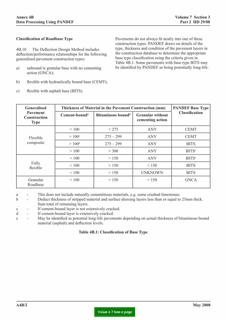
volume 7 section 3 part 2 Hd 29/08
nts depending on actual thickness of bituminous bound
tion of Base Type
annex 4B data processing using pandef
Classification of Roadbase Type
4B.10 The Deflection Design Method includes deflection/performance relationships for the following generalised pavement construction types:
a) unbound ie granular base with no cementing action (GNCA);
b) flexible with hydraulically bound base (CEMT);
c) flexible with asphalt base (BITS).
PcttbTb
generalised pavement
construction type
Thickness of Material in the Pa
Cement-bounda Bituminous
Flexible composite
> 100 < 27
> 100c 275 – 2
> 100d 275 – 2
> 100 > 30
Fully flexible
< 100 > 15
< 100 < 15
< 100 < 15
Granular Roadbase
< 100 < 15
a - This does not include naturally cementitious mb - Deduct thickness of stripped material and surfa Sum total of remaining layers. c - If cement-bound layer is not extensively cracked - If cement-bound layer is extensively cracked. e - May be identified as potential long-life paveme material (asphalt) and deflection levels.
Table 4B.1: Classifica
a4B/2
avements do not always fit neatly into one of these onstruction types. PANDEF draws on details of the ype, thickness and condition of the pavement layers in he construction database to determine the appropriate ase type classification using the criteria given in able 4B.1. Some pavements with base type BITS may e identified by PANDEF as being potentially long-life.
vement Construction (mm) pandef Base type Classification boundb granular without
cementing action
5 ANY CEMT
99 ANY CEMT
99 ANY BITS
0 ANY BITSe
0 ANY BITSe
0 < 150 BITS
0 UNKNOWN BITS
0 > 150 GNCA
aterials, e.g. some crushed limestones. ce dressing layers less than or equal to 25mm thick.
d.
may 2008
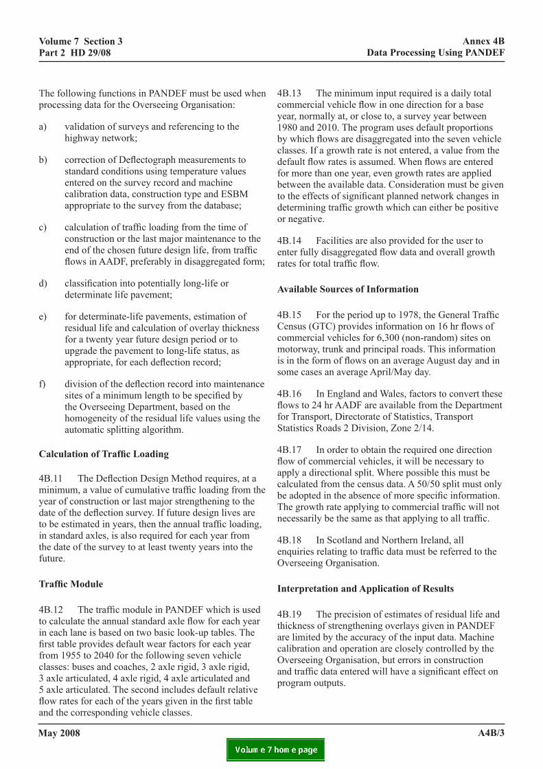
volume 7 section 3 part 2 Hd 29/08
annex 4B data processing using pandef
The following functions in PANDEF must be used when processing data for the Overseeing Organisation:
a) validation of surveys and referencing to the highway network;
b) correction of Deflectograph measurements to standard conditions using temperature values entered on the survey record and machine calibration data, construction type and ESBM appropriate to the survey from the database;
c) calculation of traffic loading from the time of construction or the last major maintenance to the end of the chosen future design life, from traffic flows in AADF, preferably in disaggregated form;
d) classification into potentially long-life or determinate life pavement;
e) for determinate-life pavements, estimation of residual life and calculation of overlay thickness for a twenty year future design period or to upgrade the pavement to long-life status, as appropriate, for each deflection record;
f) division of the deflection record into maintenance sites of a minimum length to be specified by the Overseeing Department, based on the homogeneity of the residual life values using the automatic splitting algorithm.
Calculation of Traffic Loading
4B.11 The Deflection Design Method requires, at a minimum, a value of cumulative traffic loading from the year of construction or last major strengthening to the date of the deflection survey. If future design lives are to be estimated in years, then the annual traffic loading, in standard axles, is also required for each year from the date of the survey to at least twenty years into the future.
Traffic Module
4B.12 The traffic module in PANDEF which is used to calculate the annual standard axle flow for each year in each lane is based on two basic look-up tables. The first table provides default wear factors for each year from 1955 to 2040 for the following seven vehicle classes: buses and coaches, 2 axle rigid, 3 axle rigid, 3 axle articulated, 4 axle rigid, 4 axle articulated and 5 axle articulated. The second includes default relative flow rates for each of the years given in the first table
may 2008
and the corresponding vehicle classes.
4B.13 The minimum input required is a daily total commercial vehicle flow in one direction for a base year, normally at, or close to, a survey year between 1980 and 2010. The program uses default proportions by which flows are disaggregated into the seven vehicle classes. If a growth rate is not entered, a value from the default flow rates is assumed. When flows are entered for more than one year, even growth rates are applied between the available data. Consideration must be given to the effects of significant planned network changes in determining traffic growth which can either be positive or negative.
4B.14 Facilities are also provided for the user to enter fully disaggregated flow data and overall growth rates for total traffic flow.
available sources of information
4B.15 For the period up to 1978, the General Traffic Census (GTC) provides information on 16 hr flows of commercial vehicles for 6,300 (non-random) sites on motorway, trunk and principal roads. This information is in the form of flows on an average August day and in some cases an average April/May day.
4B.16 In England and Wales, factors to convert these flows to 24 hr AADF are available from the Department for Transport, Directorate of Statistics, Transport Statistics Roads 2 Division, Zone 2/14.
4B.17 In order to obtain the required one direction flow of commercial vehicles, it will be necessary to apply a directional split. Where possible this must be calculated from the census data. A 50/50 split must only be adopted in the absence of more specific information. The growth rate applying to commercial traffic will not necessarily be the same as that applying to all traffic.
4B.18 In Scotland and Northern Ireland, all enquiries relating to traffic data must be referred to the Overseeing Organisation.
interpretation and application of results
4B.19 The precision of estimates of residual life and thickness of strengthening overlays given in PANDEF are limited by the accuracy of the input data. Machine calibration and operation are closely controlled by the Overseeing Organisation, but errors in construction and traffic data entered will have a significant effect on program outputs.
a4B/3

may 2008
volume 7 section 3 part 2 Hd 29/08
annex 5a fwd reQuirements for consistencY cHeck
Long-Term Repeatability Verification
5A.1 As well as the requirement to take part in the annual FWD correlation trial, referred to in Section 5.9, it is recommended that reassurance of the continuing consistent operation of the equipment is obtained by carrying out regular deflection and temperature measurements on a well-characterised test pavement at intervals of between four and six weeks whilst the survey equipment is in routine operation. Well-characterised means that similar tests have been carried out on the site over at least a continuous twelve month period. Ideally the test site should encompass a wide range of deflections on the three main pavement types but in reality this may not always be possible.
5A.2 Comparison of the consistency of the measured deflections, corrected for load, from each of the geophones, taking account of the measured pavement temperature and previous deflection temperature history of the site, will give an early indication of any significant faults developing that need further investigation.
a5a/1
annex 5a fwd requirements for consistency check

volume 7 section 3 part 2 Hd 29/08
deflectograpH is
eter on Pavements Part 1 – Harmonisation of FWD valuation. FEHRL Report No. 1996/1.TRL, Crowthorne,
annex 5B Falling Weight Deflectograph Surface Modulus Analaysis
annex 5B falling weigHtsurface modulus analYs
5B.1. Deflection measurements can be used to produce surface modulus plots. The surface modulus at a point, distance r from the centre of the loaded area, is roughly equal to the “weighted mean elastic stiffness” below a depth R on the load centre line. Note that the depth R is based on the “equivalent pavement thickness”, where the thickness of the pavement layers is converted to an equivalent thickness of a material with an elastic stiffness equal to the subgrade stiffness. At a point sufficiently far from the loaded area, the deflection is not influenced by the upper pavement layers. Therefore the surface modulus calculated at the outer points on the deflection bowl is approximately equal to the subgrade modulus. Such plots give an indication of the stiffness of the pavement at different equivalent depths and can be used as guidance for the selection of further investigation and analysis methods. Further details of this method are given elsewhere (FEHRL, 1996)2.
The surface modulus at the top of the pavement (equivalent depth = 0mm) is calculated as:
Eo = 2(1-ν2) σo a/δo
The surface modulus at the equivalent depth R (valid for r>2a) can be calculated from:
Eo (r) = (1-ν2) σo a2/(r.δr)
Where: Eo = the surface modulus at the centre of the loading plate (MPa) Eo (r) = the surface modulus at a distance r (MPa) ν = Poisson’s ratio σo = contact pressure under the loading plate (kPa) a = radius of the loading plate (mm) r = distance from sensor to loading centre (mm) δr = deflection at a distance r (microns)
5B.2to ascomin F
i.
ii.
iii.
iv.
v.
2 FEHRL. Harmonisation of the Use of the Falling Weight DeflectomMeasurements and Data Processing for Flexible Road Pavement E1996.
may 2008
For surface modulus analysis, it is normal sume a value of 0.35 for Poisson’s ratio. Five mon examples of surface modulus plots are shown igure 1.1:
A continuously decreasing value of surface modulus with increasing distance. This indicates that the outermost deflection measurement points were not far enough away from the load.
A decreasing value which becomes constant. This indicates a normal pavement structure overlying a linear elastic subgrade.
A decreasing value which starts to gradually increase for the outer deflection measurement points. This indicates a normal pavement structure on a non-linear elastic subgrade, or a layered subgrade which increases in stiffness with depth.
A decreasing value with a sudden large increase for the outermost measurement points. This indicates that a very stiff subgrade layer underlies the pavement (e.g. bedrock).
A minimum value close to the surface. This indicates a weak interlayer somewhere in the upper bound layers.
a5B/1
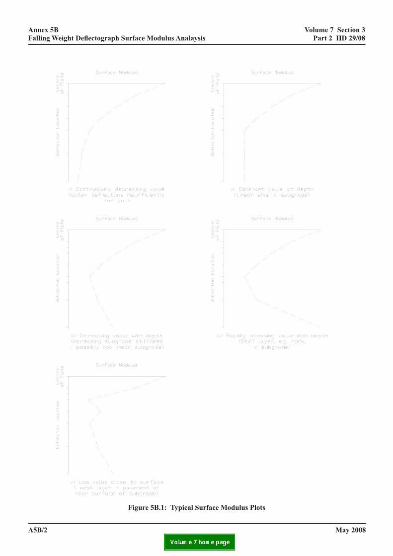
volume 7 section 3 part 2 Hd 29/08
a5B
annex 5B Falling Weight Deflectograph Surface Modulus AnalaysisAnnex 5B Volume 7 Section 3 FWD Surface Modulus Analysis Part 2 HD 29/08
A5B
figure 5B.1: typical surface modulus plots
Figure 5B.1. Typical Surface Modulus Plots.
may 2008/2/2 January 2008

volume 7 section 3 part 2 Hd 29/08
annex 5B Falling Weight Deflectograph Surface Modulus Analaysis
TEMPLATE FOR REPORTINg FWD SURVEYS AND BACK-ANALYSIS
Survey - general
Start date: . . . . . . . . . . . . . . . . . . . Finish time: . . . . . . . . . . . . .
Survey Company: . . . . . . . . . . . . . . . . . . . . . . . . . . Finish date: . . . . . . . . . . . . . . . . . . .
Operator: . . . . . . . . . . . . . . . . . . . . Start time: . . . . . . . . . . . . . .location
Road No: . . . . . . . . . . . Lane No: . . . . . Start Section: . . . . . . . . . . Ch: . . . . . . .
Location: . . . . . . . . . . . . . . . . . . . . . . . . End Section: . . . . . . . . . . Ch: . . . . . . .
Pavement type: FF / FC / Rigid Total length: . . . . . . . . . mfwd geophones
Make: . . . . . . . . . . . . Model: . . . . . . . . . . . . Type: . . . . . . . . . . . . . . . . Serial number: . . . . . . . . . . . . .
Load : . . . . . kN Plate size: . . . . . .mm Number: . . . . . . . .
Test type: Standard / LTE Positions: . . . . . . . . . . . . . . . . . . . . . . . . . .temperatures
Locations: . . . . . . . . . . . . . . . . . . . . . . . . . . Maximum temperature: . . . . . .oC
Depths (if not 100mm): . . . . . . . . . . . . . . . . .mm Minimum temperature: . . . . . .oC
Times of measurement: . . . . . . . . . . . . . . . . . .Hapms files
“Supplementary” and “F20” files attached: Yes / No survey results
1. Normalised tabulated deflection data attached: Yes / No 2. Normalised d1, [d1-d4] and d6 plots attached: Yes / No 3. Temperature data attached: Yes / Noanalysis details
Name of Program: . . . . . . . .. . . . . . . . . . . . . . . . . . . . . . Version: . . . . . . . . Mode: . . . . . . . . . . . . . . . . . . . .
No. of layers: . . . . . . Asphalt thicknesses - Max: . . . . . . . . . mm Min: . . . . . . . . . . mm Hydraulically bound mixture thicknesses - Max: . . . . . . . . . mm Min: . . . . . . . . . . mm
Sources of thickness information: Cores (No. . . . .) / GPR / As built Drgs / Other (Please specify)
Type of analysis: Standard / Non-standard (give reasons and details)analysis results
1. Tabulated back-analysed stiffnesses (at field temperature) attached: Yes / No 2. Tabulated back-analysed stiffnesses (adjusted to 20oC for asphalt layers) attached: Yes / No 3. Tabulated layer thicknesses used for each test point for analysis attached: Yes / No 4. AMD and RMS values for each test point attached: Yes / No 5. Layer stiffness (adjusted to 20oC for asphalt layers) plots attached: Yes / NoIf any data not attached please provide explanation:
may 2008 a5B/3
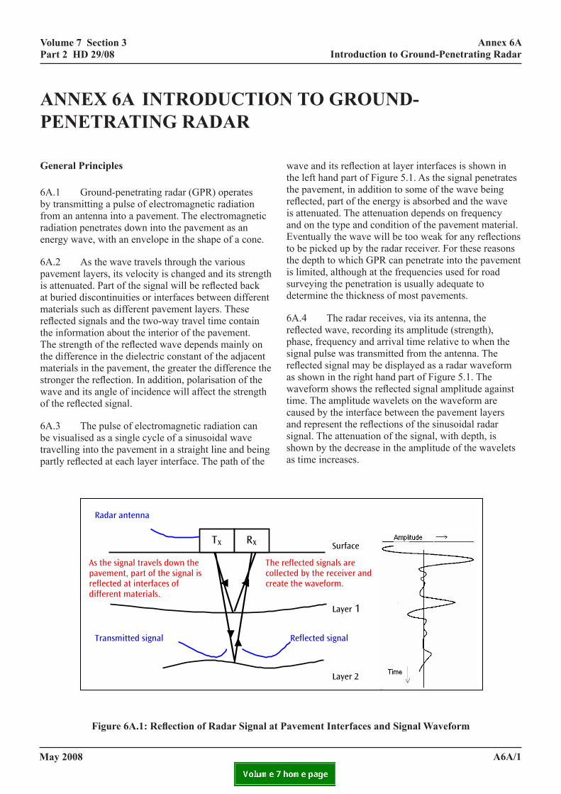
volume 7 section 3 part 2 Hd 29/08
ION TO gROUND-
nal at Pavement Interfaces and Signal Waveform
annex 6a Introduction to ground-Penetrating Radar
Volume 7 Section 3 Annex 6A Part 2 HD 29/08 Introduction to Ground-Penetrating Radar
ON TO GROUND-PENETRATING
nal at pavement interfaces and signal waveform
Reflected signal
X
Layer 1
Layer 2
Surface
The reflected signals are collected by the receiver and create the waveform.
ANNEx 6A INTRODUCTpenetrating radar
general principles
6A.1 Ground-penetrating radar (GPR) operatesby transmitting a pulse of electromagnetic radiationfrom an antenna into a pavement. The electromagnradiation penetrates down into the pavement as an energy wave, with an envelope in the shape of a co
6A.2 As the wave travels through the various pavement layers, its velocity is changed and its streis attenuated. Part of the signal will be reflected bacat buried discontinuities or interfaces between diffematerials such as different pavement layers. These reflected signals and the two-way travel time contaithe information about the interior of the pavement. The strength of the reflected wave depends mainly the difference in the dielectric constant of the adjacmaterials in the pavement, the greater the differencestronger the reflection. In addition, polarisation of twave and its angle of incidence will affect the strenof the reflected signal.
6A.3 The pulse of electromagnetic radiation cabe visualised as a single cycle of a sinusoidal wavetravelling into the pavement in a straight line and bpartly reflected at each layer interface. The path of
Figure 6A.1: Reflection of Radar Sig
ANNEX 6A – INTRODUCTIRADAR General Principles
6A.1 Ground-penetrating radar (GPR) operates byantenna into a pavement. The electromagnetic radiaan envelope in the shape of a cone.
6A.2 As the wave travels through the various paveattenuated. Part of the signal will be reflected back materials such as different pavement layers. These information about the interior of the pavement. Thein the dielectric constant of the adjacent materials inreflection. In addition, polarisation of the wave andsignal.
6A.3 The pulse of electromagnetic radiation can bthe pavement in a straight line and being partly reflreflection at layer interfaces is shown in the left hanaddition to some of the wave being reflected, part oattenuation depends on frequency and on the type abe too weak for any reflections to be picked up by tpenetrate into the pavement is limited, although at tusually adequate to determine the thickness of mos
6A.4 The radar receives, via its antenna, the reflecand arrival time relative to when the signal pulse wadisplayed as a radar waveform as shown in the righsignal amplitude against time. The amplitude wavepavement layers and represent the reflections of thedepth, is shown by the decrease in the amplitude of
Figure 6A.1 Reflection of radar sig
As the signal travels down the pavement, part of the signal is reflected at interfaces of different materials.
Transmitted signal
T X R
Radar antenna
may 2008January 2008
etic
ne.
ngth k rent
n
on ent the
he gth
n eing the
wave and its reflection at layer interfaces is shown in the left hand part of Figure 5.1. As the signal penetrates the pavement, in addition to some of the wave being reflected, part of the energy is absorbed and the wave is attenuated. The attenuation depends on frequency and on the type and condition of the pavement material. Eventually the wave will be too weak for any reflections to be picked up by the radar receiver. For these reasons the depth to which GPR can penetrate into the pavement is limited, although at the frequencies used for road surveying the penetration is usually adequate to determine the thickness of most pavements.
6A.4 The radar receives, via its antenna, the reflected wave, recording its amplitude (strength), phase, frequency and arrival time relative to when the signal pulse was transmitted from the antenna. The reflected signal may be displayed as a radar waveform as shown in the right hand part of Figure 5.1. The waveform shows the reflected signal amplitude against time. The amplitude wavelets on the waveform are caused by the interface between the pavement layers and represent the reflections of the sinusoidal radar signal. The attenuation of the signal, with depth, is shown by the decrease in the amplitude of the wavelets as time increases.
transmitting a pulse of electromagnetic radiation from an tion penetrates down into the pavement as an energy wave, with
ment layers, its velocity is changed and its strength is at buried discontinuities or interfaces between different reflected signals and the two-way travel time contain the strength of the reflected wave depends mainly on the difference the pavement, the greater the difference the stronger the
its angle of incidence will affect the strength of the reflected
e visualised as a single cycle of a sinusoidal wave travelling into ected at each layer interface. The path of the wave and its d part of Figure 5.1. As the signal penetrates the pavement, in f the energy is absorbed and the wave is attenuated. The nd condition of the pavement material. Eventually the wave will he radar receiver. For these reasons the depth to which GPR can he frequencies used for road surveying the penetration is t pavements.
ted wave, recording its amplitude (strength), phase, frequency s transmitted from the antenna. The reflected signal may be t hand part of Figure 5.1. The waveform shows the reflected lets on the waveform are caused by the interface between the sinusoidal radar signal. The attenuation of the signal, with the wavelets as time increases.
a6a/1A6A/1
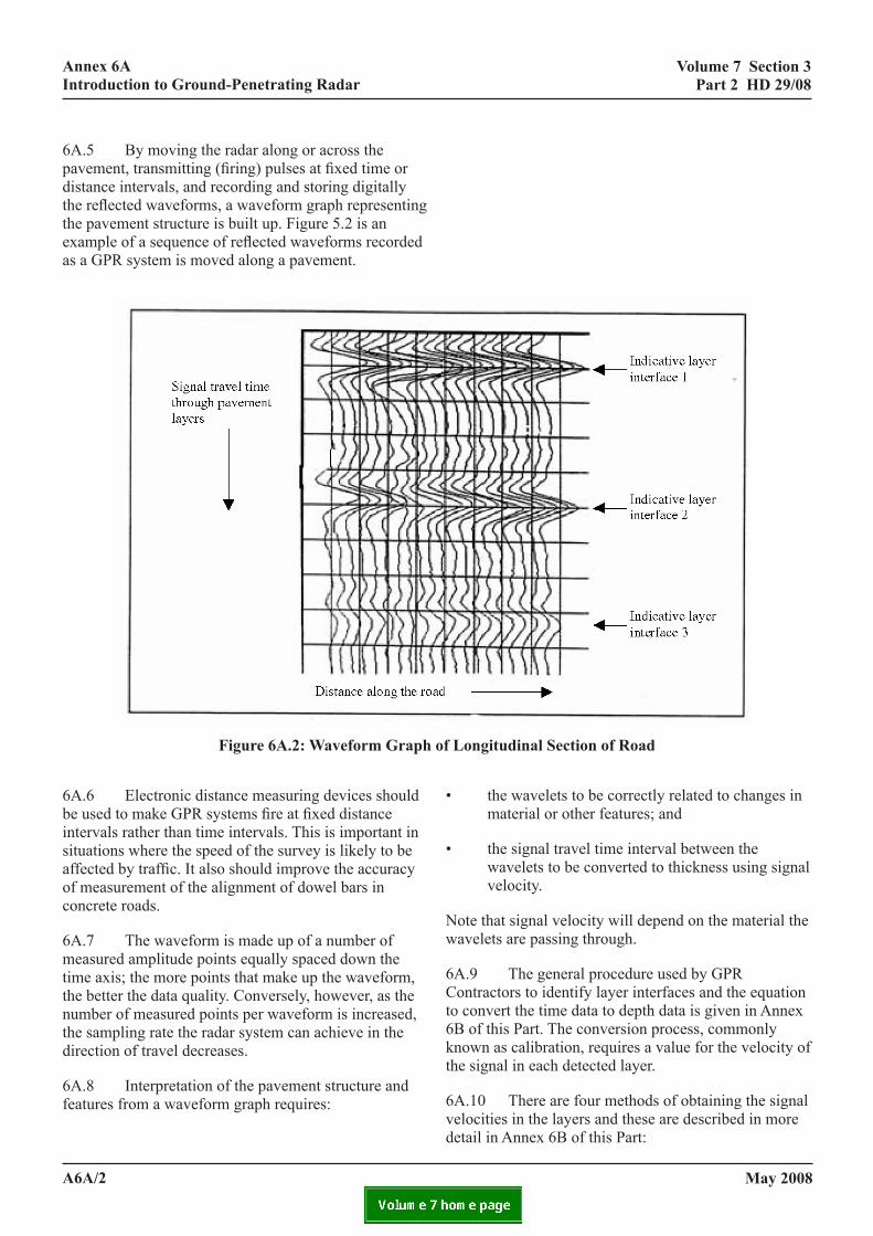
volume 7 section 3 part 2 Hd 29/08
annex 6a Introduction to ground-Penetrating Radar
Volume 7 Section 3 Part 2 HD 29/08
transmitting (firing) pulses at fixed time or distance waveforms, a waveform graph representing the pavement ce of reflected waveforms recorded as a GPR system is
6A.5 By moving the radar along or across the pavement, transmitting (firing) pulses at fixed time or distance intervals, and recording and storing digitally the reflected waveforms, a waveform graph representingthe pavement structure is built up. Figure 5.2 is an example of a sequence of reflected waveforms recorded as a GPR system is moved along a pavement.
figure 6a.2: waveform graph
6A.6 Electronic distance measuring devices should be used to make GPR systems fire at fixed distance intervals rather than time intervals. This is important in situations where the speed of the survey is likely to be affected by traffic. It also should improve the accuracy of measurement of the alignment of dowel bars in concrete roads.
6A.7 The waveform is made up of a number of measured amplitude points equally spaced down the time axis; the more points that make up the waveform, the better the data quality. Conversely, however, as the number of measured points per waveform is increased, the sampling rate the radar system can achieve in the direction of travel decreases.
6A.8 Interpretation of the pavement structure and features from a waveform graph requires:
Annex 6A Introduction to Ground-Penetrating Radar
6A.5 By moving the radar along or across the pavement,intervals, and recording and storing digitally the reflectedstructure is built up. Figure 5.2 is an example of a sequenmoved along a pavement.
Figure 6A.2 Waveform graph
6A.6 Electronic distance measuring devices should be usrather than time intervals. This is important in situations wtraffic. It also should improve the accuracy of measurem
6A.7 The waveform is made up of a number of measuredmore points that make up the waveform, the better the datpoints per waveform is increased the sampling rate the rad
6A.8 Interpretation of the pavement structure and feature
• the wavelets to be correctly related to changes in m
• the signal travel time interval between the wavelets
Note that signal velocity will depend on the material the w
a6a/2
A6A/2
may 2008
of longitudinal section of road
• the wavelets to be correctly related to changes in material or other features; and
• the signal travel time interval between the wavelets to be converted to thickness using signal velocity.
Note that signal velocity will depend on the material the wavelets are passing through.
6A.9 The general procedure used by GPR Contractors to identify layer interfaces and the equation to convert the time data to depth data is given in Annex 6B of this Part. The conversion process, commonly known as calibration, requires a value for the velocity of the signal in each detected layer.
6A.10 There are four methods of obtaining the signal velocities in the layers and these are described in more detail in Annex 6B of this Part:
of longitudinal section of road
ed to make GPR systems fire at fixed distance intervals here the speed of the survey is likely to be affected by
ent of the alignment of dowel bars in concrete roads.
amplitude points equally spaced down the time axis; the a quality. Conversely however as the number of measured ar system can achieve in the direction of travel decreases.
s from a waveform graph requires:
aterial or other features; and
to be converted to thickness using signal velocity.
avelets are passing through.
January 2008
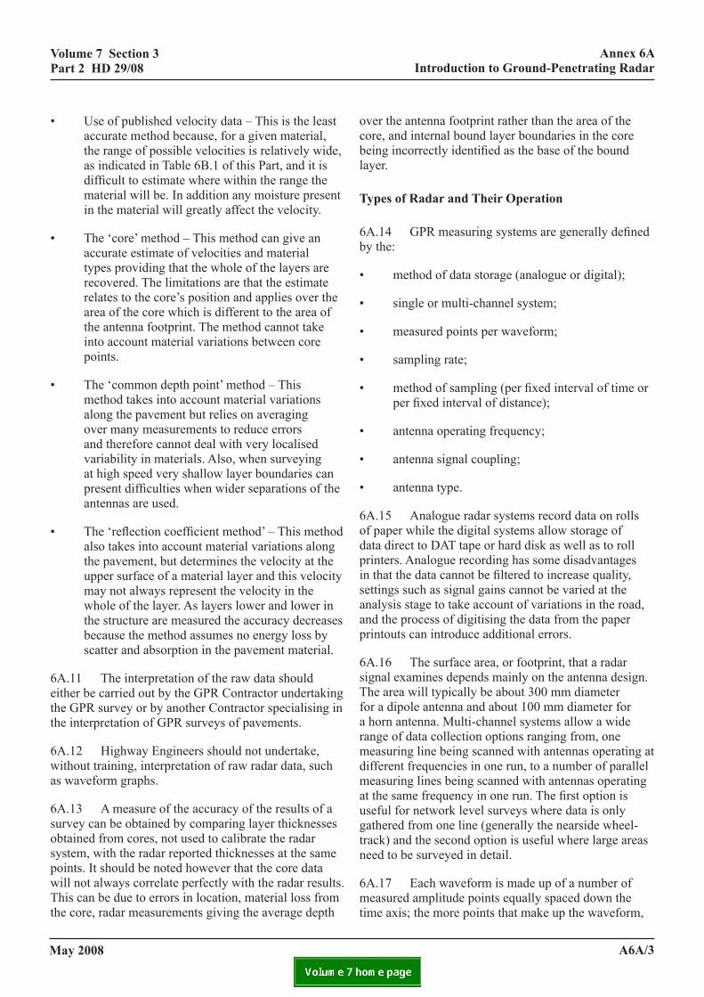
volume 7 section 3 part 2 Hd 29/08
annex 6a Introduction to ground-Penetrating Radar
• Use of published velocity data – This is the least accurate method because, for a given material, the range of possible velocities is relatively wide, as indicated in Table 6B.1 of this Part, and it is difficult to estimate where within the range the material will be. In addition any moisture present in the material will greatly affect the velocity.
• The ‘core’ method – This method can give an accurate estimate of velocities and material types providing that the whole of the layers are recovered. The limitations are that the estimate relates to the core’s position and applies over the area of the core which is different to the area of the antenna footprint. The method cannot take into account material variations between core points.
• The ‘common depth point’ method – This method takes into account material variations along the pavement but relies on averaging over many measurements to reduce errors and therefore cannot deal with very localised variability in materials. Also, when surveying at high speed very shallow layer boundaries can present difficulties when wider separations of the antennas are used.
• The ‘reflection coefficient method’ – This method also takes into account material variations along the pavement, but determines the velocity at the upper surface of a material layer and this velocity may not always represent the velocity in the whole of the layer. As layers lower and lower in the structure are measured the accuracy decreases because the method assumes no energy loss by scatter and absorption in the pavement material.
6A.11 The interpretation of the raw data should either be carried out by the GPR Contractor undertaking the GPR survey or by another Contractor specialising in the interpretation of GPR surveys of pavements.
6A.12 Highway Engineers should not undertake, without training, interpretation of raw radar data, such as waveform graphs.
6A.13 A measure of the accuracy of the results of a survey can be obtained by comparing layer thicknesses obtained from cores, not used to calibrate the radar system, with the radar reported thicknesses at the same points. It should be noted however that the core data will not always correlate perfectly with the radar results. This can be due to errors in location, material loss from the core, radar measurements giving the average depth
may 2008
over the antenna footprint rather than the area of the core, and internal bound layer boundaries in the core being incorrectly identified as the base of the bound layer.
types of radar and their operation
6A.14 GPR measuring systems are generally defined by the:
• method of data storage (analogue or digital);
• single or multi-channel system;
• measured points per waveform;
• sampling rate;
• method of sampling (per fixed interval of time or per fixed interval of distance);
• antenna operating frequency;
• antenna signal coupling;
• antenna type.
6A.15 Analogue radar systems record data on rolls of paper while the digital systems allow storage of data direct to DAT tape or hard disk as well as to roll printers. Analogue recording has some disadvantages in that the data cannot be filtered to increase quality, settings such as signal gains cannot be varied at the analysis stage to take account of variations in the road, and the process of digitising the data from the paper printouts can introduce additional errors.
6A.16 The surface area, or footprint, that a radar signal examines depends mainly on the antenna design. The area will typically be about 300 mm diameter for a dipole antenna and about 100 mm diameter for a horn antenna. Multi-channel systems allow a wide range of data collection options ranging from, one measuring line being scanned with antennas operating at different frequencies in one run, to a number of parallel measuring lines being scanned with antennas operating at the same frequency in one run. The first option is useful for network level surveys where data is only gathered from one line (generally the nearside wheel-track) and the second option is useful where large areas need to be surveyed in detail.
6A.17 Each waveform is made up of a number of measured amplitude points equally spaced down the time axis; the more points that make up the waveform,
a6a/3
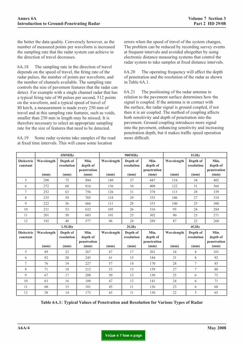
volume 7 section 3 part 2 Hd 29/08
annex 6a Introduction to ground-Penetrating Radar
olution
(mm)
depth of penetration
(mm)
(mm)
resolution
(mm)
depth of penetration
(mm)37 447 134 34 40234 408 122 31 36631 378 113 28 33929 353 106 27 31828 333 100 25 30026 316 95 24 28425 302 90 23 27124 289 87 22 260
gHz 4gHzepth of olution
(mm)
min. depth of
penetration (mm)
wavelength
(mm)
depth of resolution
(mm)
min. depth of
penetration (mm)
17 201 34 8 10115 184 31 8 9214 170 28 7 8513 159 27 7 8013 150 25 6 7512 141 24 6 7111 136 23 6 6811 130 22 5 65
resolution for various types of radar
the better the data quality. Conversely however, as the number of measured points per waveform is increased the sampling rate that the radar system can achieve in the direction of travel decreases.
6A.18 The sampling rate in the direction of travel depends on the speed of travel, the firing rate of the radar pulses, the number of points per waveform, and the number of channels available. The sampling rate controls the size of pavement features that the radar can detect. For example with a single channel radar that has a typical firing rate of 90 pulses per second, 512 points on the waveform, and a typical speed of travel of 80 km/h, a measurement is made every 250 mm of travel and at this sampling rate features, such as voids, smaller than 250 mm in length may be missed. It is therefore necessary to select an appropriate sampling rate for the size of features that need to be detected.
6A.19 Some radar systems take samples of the road at fixed time intervals. This will cause some location
erThatelra
6Aofin
6Aresigththbopainpem
450mHz 90dielectric constant
wavelength
(mm)
depth of resolution
(mm)
min. depth of
penetration (mm)
wavelength
(mm)
dres
5 298 75 894 1496 272 68 816 1367 252 63 756 1268 235 59 705 1189 222 56 666 11110 211 53 632 10511 201 50 603 10112 192 48 577 96
1.5gHz 2dielectric constant
wavelength
(mm)
depth of resolution
(mm)
min. depth of
penetration (mm)
wavelength
(mm)
dres
5 89 22 267 676 82 20 245 617 76 19 227 578 71 18 212 539 67 17 200 5010 63 16 189 4711 60 15 181 4512 58 14 173 43
table 6a.1: typical values of penetration and
a6a/4
rors when the speed of travel of the system changes, e problem can be reduced by recording survey events
frequent intervals and avoided altogether by using ectronic distance measuring systems that control the dar system to take samples at fixed distance intervals.
.20 The operating frequency will affect the depth penetration and the resolution of the radar as shown Table 6A.1.
.21 The positioning of the radar antenna in lation to the pavement surface determines how the nal is coupled. If the antenna is in contact with
e surface, the radar signal is ground coupled, if not en it is air coupled. The method of coupling affects th sensitivity and depth of penetration into the vement. Ground coupling introduces more signal to the pavement, enhancing sensitivity and increasing netration depth, but it makes traffic speed operation ore difficult.
0mHz 1gHzepth of min. wavelength depth of min.
may 2008

volume 7 section 3 part 2 Hd 29/08
annex 6a Introduction to ground-Penetrating Radar
6A.22 There are two types of antenna design, dipoles and horns. Dipoles operate most effectively when they are ground coupled, however, they can be air coupled but the gap between the antenna and pavement surface has to be small, ideally one-tenth of the transmitted wavelength to give satisfactory results. This means that the antenna mounting has to be carefully designed to enable surveys to be done at traffic speed. Horn antennas are air coupled and operate with a large air gap and so are more easily adapted to surveys at traffic speed.
6A.23 Radar can be used to detect other features such as buried services and drains but this is outside the scope of this Annex.
6A.24 Depending on the coupling and design of the radar system, a survey can either be carried out at low speed, typically between 0.5 and 20 km/h, or at traffic speed, typically between 50 and 80 km/h. Figure 6A.3 illustrates radar systems operating over this range of survey speeds. The sampling rate, in the direction of travel, achieved with high speed surveys will be lower so only larger features will be detected.
may 2008 a6a/5

volume 7 section 3 part 2 Hd 29/08
annex 6a Introduction to ground-Penetrating Radar
Radar with ground Coupled Dipole Sntenna – Crack Depth Investigation at 0.5 km/h surveying at 0.5 km/h
Radar with Horn Antenna – Surveying at 80 km/h Radar with a Pair of Air-Coupled Dipole Antennas – surveying at 80 km/h
Figure 6A.3 ground-Penetrating Radar Systems
may 2008a6a/6
volume 7 section 3 part 2 Hd 29/08
f gpr for r tHickness
annex 6B calibration of gpr for determination of layer thickness
annex 6B caliBration odetermination of laYe
general
6B.1 This annex gives details of the methods used by the GPR Contractors to determine the thickness of the pavement layers from the radar data. The information is presented to illustrate the strengths and weakness of the different approaches.
6B.2 The process of determining the layer thicknesses from a GPR waveform is carried out in two stages:
• identifying layer interface wavelets on the waveform;
• using the times between the wavelets to calculate the layer thicknesses.
Stage 1 – Identifying Layer Interface Wavelets
6B.3 The layer interfaces appear on the waveform as wavelets and the following processes are carried out to identify and characterise all the layer interface wavelets:
• relate wavelets to material boundaries (it may be necessary to filter the data to clearly resolve the wavelets);
• track along pavement, wavelets relating to material boundary;
• record time to wavelet at each sample point along the pavement;
• repeat the above processes for all material boundaries forming the pavement.
While it is theoretically possible to carry out the above processes manually it is very impractical to do this due to the excessive time required and associated high cost incurred. The processes are much more accurately and rapidly carried out with a computer system that can automatically track clear boundaries but can be manually overridden, e.g. with a mouse pointer, where the signals are difficult to track automatically.
may 2008
Stage 2 – Calculating Layer Thickness
6B.4 The thickness of a layer is related to the signal travel time in the layer by the equation:
=
2T T D ...........................................................(1)
where:
D = layer thickness (mm); V = velocity of radar signal in layer (mm/ns); T = two way travel time of the signal in layer (ns).
Two way travel time of the signal in the layer is the time interval between the wavelets occurring at the layer’s lower and upper interfaces at the same location along the pavement.
signal velocity in layer
6B.5 The velocity of the radar signal within a layer is related to the layer material’s dielectric constant ε by the equation:
ε=
299 V .................................................................(2)
where:
V = velocity of radar signal in layer (mm/ns).
There are four basic methods of calculating velocities:
(a) use published data of mean velocities of pavement materials;
(b) use cores to establish layer thicknesses and then calculate velocities by rearranging equation (1) above;
(c) calculate velocity from recorded radar signal using ‘common depth point’ method;
(d) calculate velocity from recorded radar signal using ‘reflection coefficient’ method.
a6B/1
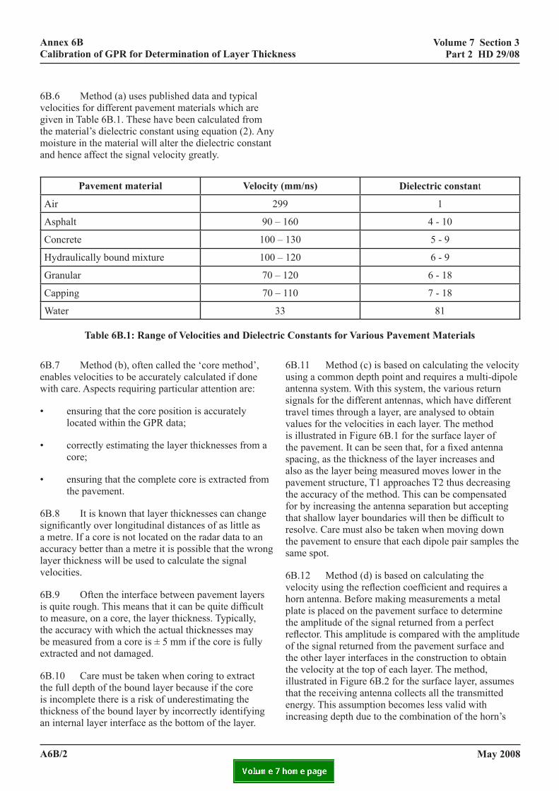
volume 7 section 3 part 2 Hd 29/08
y (mm/ns) dielectric constant
299 1
– 160 4 - 10
– 130 5 - 9
– 120 6 - 9
– 120 6 - 18
– 110 7 - 18
33 81
annex 6B calibration of gpr for determination of layer thickness
6B.6 Method (a) uses published data and typical velocities for different pavement materials which are given in Table 6B.1. These have been calculated from the material’s dielectric constant using equation (2). Anymoisture in the material will alter the dielectric constant and hence affect the signal velocity greatly.
pavement material Velocit
Air
Asphalt 90
Concrete 100
Hydraulically bound mixture 100
Granular 70
Capping 70
Water
table 6B.1: range of velocities and dielect
6B.7 Method (b), often called the ‘core method’, enables velocities to be accurately calculated if done with care. Aspects requiring particular attention are:
• ensuring that the core position is accurately located within the GPR data;
• correctly estimating the layer thicknesses from a core;
• ensuring that the complete core is extracted from the pavement.
6B.8 It is known that layer thicknesses can change significantly over longitudinal distances of as little as a metre. If a core is not located on the radar data to an accuracy better than a metre it is possible that the wronglayer thickness will be used to calculate the signal velocities.
6B.9 Often the interface between pavement layers is quite rough. This means that it can be quite difficult to measure, on a core, the layer thickness. Typically, the accuracy with which the actual thicknesses may be measured from a core is ± 5 mm if the core is fully extracted and not damaged.
6B.10 Care must be taken when coring to extract the full depth of the bound layer because if the core is incomplete there is a risk of underestimating the thickness of the bound layer by incorrectly identifying an internal layer interface as the bottom of the layer.
a6B/2
ric constants for various pavement materials
6B.11 Method (c) is based on calculating the velocity using a common depth point and requires a multi-dipole antenna system. With this system, the various return signals for the different antennas, which have different travel times through a layer, are analysed to obtain values for the velocities in each layer. The method is illustrated in Figure 6B.1 for the surface layer of the pavement. It can be seen that, for a fixed antenna spacing, as the thickness of the layer increases and also as the layer being measured moves lower in the pavement structure, T1 approaches T2 thus decreasing the accuracy of the method. This can be compensated for by increasing the antenna separation but accepting that shallow layer boundaries will then be difficult to resolve. Care must also be taken when moving down the pavement to ensure that each dipole pair samples the same spot.
6B.12 Method (d) is based on calculating the velocity using the reflection coefficient and requires a horn antenna. Before making measurements a metal plate is placed on the pavement surface to determine the amplitude of the signal returned from a perfect reflector. This amplitude is compared with the amplitude of the signal returned from the pavement surface and the other layer interfaces in the construction to obtain the velocity at the top of each layer. The method, illustrated in Figure 6B.2 for the surface layer, assumes that the receiving antenna collects all the transmitted energy. This assumption becomes less valid with increasing depth due to the combination of the horn’s
may 2008
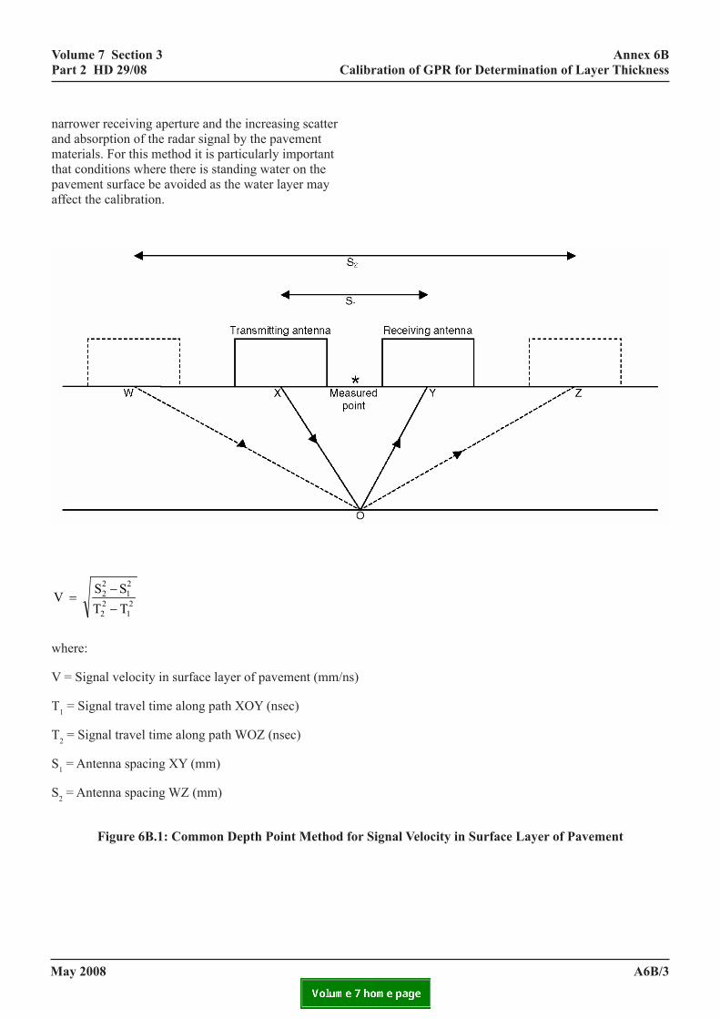
volume 7 section 3 part 2 Hd 29/08
er of pavement
annex 6B calibration of gpr for determination of layer thickness
Volume 7 Section 3 Part 2 HD 29/08
of pavement
narrower receiving aperture and the increasing scatter and absorption of the radar signal by the pavement materials. For this method it is particularly important that conditions where there is standing water on the pavement surface be avoided as the water layer may affect the calibration.
21
22
21
22
TTSS V
−−
=
where:
V = Signal velocity in surface layer of pavement (mm/ns)
T1 = Signal travel time along path XOY (nsec)
T2 = Signal travel time along path WOZ (nsec)
S1 = Antenna spacing XY (mm)
S2 = Antenna spacing WZ (mm)
figure 6B.1: common depth point method for signal velocity in surface lay
Annex 6B Calibration of GPR for Determination of Layer Thickness
21
22
21
22
TTSS V
where:
V = Signal velocity in surface layer of pavement (mm/ns)
T1 = Signal travel time along path XOY (nsec)
T2 = Signal travel time along path WOZ (nsec)
S1 = Antenna spacing XY (mm)
S2 = Antenna spacing WZ (mm)
Figure 6B.1 Common depth point method for signal velocity in surface layer
may 2008 a6B/3
A6B/4 January 2008
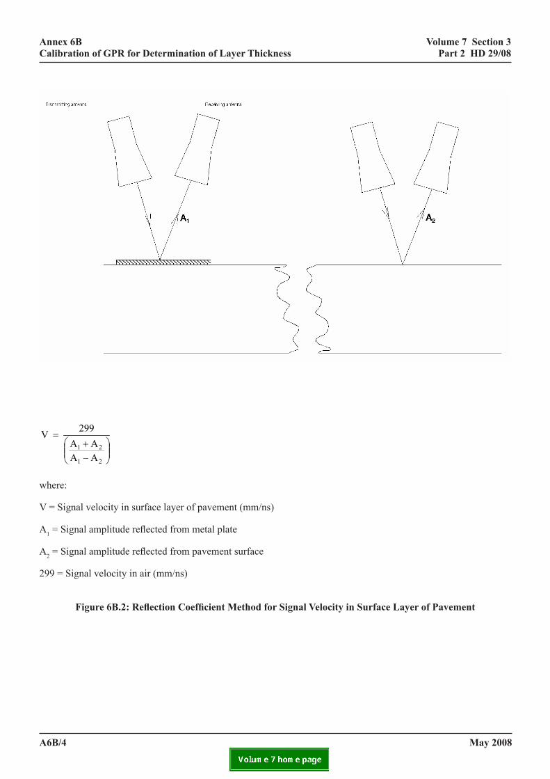
volume 7 section 3 part 2 Hd 29/08
annex 6B calibration of gpr for determination of layer thicknessVolume 7 Section 3 Annex 6B Part 2 HD 29/08 Calibration of GPR for Determination of Layer Thickness
−+
=
21
21
AAAA
299 V
where:
V = Signal velocity in surface layer of pavement (mm/ns)
A1 = Signal amplitude reflected from metal plate
A2 = Signal amplitude reflected from pavement surface
299 = Signal velocity in air (mm/ns)
Figure 6B.2: Reflection Coefficient Method for Signal Velocity in Surface Layer of Pavement
21
21
AAAA
299 V
where:
V = Signal velocity in surface layer of pavement (mm/ns)
A1 = Signal amplitude reflected from metal plate
A2 = Signal amplitude reflected from pavement surface
299 = Signal velocity in air (mm/ns)
Figure 6B.2 Reflection coefficient method for signal velocity in surface layer of pavement
may 2008a6B/4January 2008 A6B/1

may 2008
volume 7 section 3 part 2 Hd 29/08
annex 6c reporting tHe results of a gROUND-PENETRATINg RADAR SURVEY
6C.1 Examples of how the data may be presented in graphical form and tabular form are shown in Figure 6C.1 and Tables 6C.1 and 6C.2.
a6c/1
annex 6c Reporting the Results of a ground-Penetrating Radar Survey
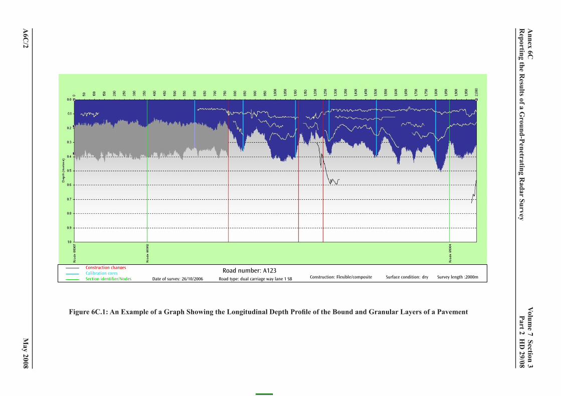
may 2008
volume 7 section 3
part 2 Hd
29/08
Figure 6C.1: An Example of a graph Showing the Longitudinal Depth Profile of the Bound and granular Layers of a Pavement
a6c
/2
annex 6c
R
eporting the Results of a g
round-Penetrating Radar Survey
Volume 7 Section 3 Annex 6C Part 2 HD 29/08 Reporting the Results of a GPR Survey
January 2008 A6C/1
ANNEX 6C. REPORTING THE RESULTS OF A GROUND-PENETRATING RADAR SURVEY 6C.1 Examples of how the data may be presented in graphical form and tabular form are shown in Figure 6C.1 and Tables 6C.1 and 6C.2.
Figure 6C.1 An example of a graph showing the longitudinal depth profile of the bound and granular layers of a pavement
Construction changes Calibration cores Section identifier/Nodes
Road number: A123Date of survey: 26/10/2006 Road type: dual carriage way lane 1 SB Construction: Flexible/composite Survey length :2000m Surface condition: dry

may 2008
volume 7 section 3 part 2 Hd 29/08
Network section identifier: 600A123 12 lane/s surveyed and track: Nearside lane, nearside wheel-track
road number: A123
date of survey: 19-6-2006 length surveyed: 900 m
direction of survey: South
road type: Dual 2 lane APTR surface moisture condition: Dry
construction: Flexible with asphalt base
chainage from start of network
section (m)
Bound layer depth (mm)
granular layer depth (mm)
comments (defect features, construction changes and core information)
100 245 225
200 245 220
300 250 215 Calibration core taken from nearside wheel-track at chainage 320m
400 255 215
500 255 210
600 250 210
Table 6C.1: An Example of How Layer Thickness Data from a gPR Survey Should be Presented
Network section identifier: 1900M21 10 lane/s surveyed and track: Nearside lane, nearside wheel-track
road number: M21
date of survey: 19-6-2006 length surveyed: 1200 m
direction of survey: South
road type: Dual 2 lane motorway surface moisture condition: Damp no standing water
construction: Concrete
chainage from start of network
section (m)
Bound layer depth (mm)
granular layer depth
(mm)
Comments (defect features, construction changes and core information)
120 260 180 Indications that some dowel bars are misaligned
130 260 175
140 260 180
150 270 180 Possible void starting about 2 m from nearside edge of lane, approximate area 2 x 1.5 m. Indications that some dowel bars within area of void are too close to the surface
160 270 180
170 270 180
180 280 175
190 280 175
Table 6C.2: An Example of How the gPR Survey Data for a Concrete Pavement Should be Presented
a6c/3
annex 6c Reporting the Results of a ground-Penetrating Radar Survey