dlubal-tutorial

Program RSBUCK © 2011 Ing.-Software Dlubal

Add-on Module

RSBUCK Buckling Lengths, Buckling Shapes, Critical Load Factors

Program Description

Version March 2011

All rights, including those of translations, are reserved.

No portion of this book may be reproduced – mechanically, electronically, or by any other means, including photocopying – without written permission of ING.-SOFTWARE DLUBAL. © Ing.-Software Dlubal Am Zellweg 2 D-93464 Tiefenbach

Tel.: +49 (0) 9673 9203-0 Fax: +49 (0) 9673 9230-51 E-mail: [email protected] Web: www.dlubal.com

3 Program RSBUCK © 2011 Ing.-Software Dlubal

Contents

Contents Page

Contents Page

1. Introduction 4 1.1 Add-on Module RSBUCK 4 1.2 RSBUCK Team 5 1.3 Using the Manual 5 1.4 Open the Add-on Module RSBUCK 6 2. Input Data 8 2.1 General Data 8 2.2 Axial Forces 11 3. Calculation 12 3.1 Check 12 3.2 Start Calculation 13 4. Results 14 4.1 Buckling Lengths and Loads 15 4.2 Buckling Shapes 16 4.3 Critical Load Factors 18 5. Results Evaluation 20 5.1 Results Tables 20

5.2 Results Graphic 21 5.3 Filter for Results 23 5.4 Non-linear RSTAB Calculation 24 6. Printout 25 6.1 Printout Report 25 6.2 Print RSBUCK Graphics 26 7. General Functions 27 7.1 RSBUCK Analysis Cases 27 7.2 Units and Decimal Places 29 7.3 Export of Results 29 8. Examples 32 8.1 Euler Buckling Mode 1 32 8.2 Frame with K-Bracing 35 8.3 Frame with Hinged Column 38 A Literature 40 B Index 41

1 Introduction


1. Introduction

1.1 Add-on Module RSBUCK The RSTAB add-on module RSBUCK determines the critical load factors and corresponding buckling shapes for frameworks. They represent the basis for the stability analysis, which must often be performed in addition to the general stress design, for structural parts sub-jected to compression.

The critical load factor (bifurcation load factor of the entire structure) is a value indicating the stability risk of the structural system. The respective buckling mode gives you informa-tion about the risk-bearing area in the structural model. With the add-on module RSBUCK you can analyze several buckling shapes simultaneously. The decisive failure modes of the calculated structural component are shown in the results output, sorted by the critical load factor.

Due to the graphical representation of buckling shapes you can easily detect the areas bear-ing instability risks and, if necessary, derive structural measures in order to deal with those modes of failure. Therefore, RSBUCK is a useful tool for the analysis of structures with a high risk for buckling, in particular slender beams and space frames: On the one hand, you can use the critical load factor to evaluate if the system is generally prone to instability risks (buckling and lateral-torsional buckling). On the other hand, once the critical (lowest) buck-ling shapes are determined, you can derive imperfection loads.

RSBUCK provides the following specific features:

• Simultaneous determination of several buckling shapes in one calculation run

• Automatic import of axial forces of a load case or group from RSTAB

• Option to take into account favorable effects due to tension

• Efficient equation solver for eigenvalue analysis according to subspace iteration me-thod with user-definable parameters

• Tabular output of critical buckling load factors and corresponding buckling modes

• Visualization of buckling shapes with animation option in the RSTAB graphical user interface

• Integration in RSTAB printout report with automatic update of all modifications

• Option to use buckling modes in the add-on modules RSIMP, KAPPA and TIMBER Pro

• Data export to MS Excel and OpenOffice.org Calc or as a CSV file

We hope you will enjoy working with RSBUCK.

Your team from ING.-SOFTWARE DLUBAL

1 Introduction


1.2 RSBUCK Team The following people were involved in the development of RSBUCK:

Program coordination Dipl.-Ing. Georg Dlubal Dipl.-Ing. (FH) Younes El Frem

Programming Dr.-Ing. Jaroslav Lain Ing. Michal Balvon

Ing. Roman Svoboda

Program design Dipl.-Ing. Georg Dlubal Ing. Jan Miléř

Program supervision Ing. Martin Vasek Ing. Václav Rek

Manual, help system and translation Dipl.-Ing. Frank Faulstich Dipl.-Ing. (FH) Robert Vogl Ing. Ladislav Kábrt

Mgr. Michaela Kryšková Dipl.-Ü. Gundel Pietzcker Mgr. Petra Pokorná

Technical support and quality management Dipl.-Ing. (BA) Markus Baumgärtel Dipl.-Ing. (BA) Sandy Baumgärtel Dipl.-Ing. (FH) Steffen Clauß Dipl.-Ing. (FH) Matthias Entenmann Dipl.-Ing. Frank Faulstich Dipl.-Ing. (FH) René Flori Dipl.-Ing. (FH) Stefan Frenzel Dipl.-Ing. (FH) Walter Fröhlich Dipl.-Ing. (FH) Andreas Hörold

Dipl.-Ing. (FH) Bastian Kuhn M.Sc. Dipl.-Ing. Frank Lobisch Dipl.-Ing. (FH) Alexander Meierhofer M.Eng. Dipl.-Ing. (BA) Andreas Niemeier M.Eng. Dipl.-Ing. (FH) Walter Rustler M.Sc. Dipl.-Ing. (FH) Frank Sonntag Dipl.-Ing. (FH) Christian Stautner Dipl.-Ing. (FH) Robert Vogl Dipl.-Ing. (FH) Andreas Wopperer

1.3 Using the Manual Topics like installation, graphical user interface, results evaluation and printout are de-scribed in detail in the manual of the main program RSTAB. The present manual focuses on typical features of the RSBUCK add-on module.

The descriptions in this manual follow the sequence of the module's input and results tables as well as their structure. The text of the manual shows the described buttons in square brackets, for example [New]. At the same time, they are pictured on the left. In addition, expressions used in dialog boxes, tables and menus are set in italics to clarify the explana-tions.

Finally, you find an index at the end of the manual. However, if you don’t find what you are looking for, please check our website www.dlubal.com where you can go through our FAQ pages.

1 Introduction


1.4 Open the Add-on Module RSBUCK RSTAB provides the following options to start the add-on module RSBUCK.

Menu To start the program in the menu bar,

point to Stability on the Additional Modules menu, and then select RSBUCK.

Figure 1.1: Menu: Additional Modules → Stability → RSBUCK

Navigator To start RSBUCK in the Data navigator,

select RSBUCK in the Additional Modules folder.

Figure 1.2: Data navigator: Additional Modules → RSBUCK

1 Introduction


Panel In case RSBUCK results are already available in the RSTAB structure, you can set the relevant RSBUCK case in the load case list of the RSTAB toolbar. Activate the button [Results on/off] to display the stability mode graphically in the model.

When the results display is activated, the panel appears showing the button [RSBUCK] which you can use to open the add-on module.

Figure 1.3: Panel button [RSBUCK]

2 Input Data


2. Input Data When you have started RSBUCK, a new window opens where a navigator is displayed on the left, managing all input and results tables that can be selected currently. The pull-down list above the navigator contains the stability cases that are already available (see chapter 7.1, page 27).

If you open RSBUCK in an RSTAB structure for the first time, the module will import the created load cases and load groups automatically.

To select a table, click the corresponding entry in the RSBUCK navigator or page through the tables by using the buttons shown on the left. You can also use the function keys [F2] and [F3] to select the previous or subsequent table.

To save the defined settings and quit the module, click [OK]. When you click [Cancel], you quit the module but without saving the data.

Usually, it is sufficient to enter all input data required for the definition of stability cases in the first input table.

2.1 General Data In table 1.1 General Data, you define the parameters for the buckling analysis.

Figure 2.1: Table 1.1 General Data

General Number of Buckling Shapes RSBUCK determines the most unfavorable buckling shapes of a structure. With the number entered in the input field you specify how many shapes will be determined. On principle, the upper limit is defined by 10,000 of the lowest eigenvalues of a structure, provided that it is allowed by the number of possible degrees of freedom in the model as well as by the RAM capacity.

2 Input Data


Generally, the theory forming the calculation method's basis does not allow for an exclusion of the low eigenvalues from the analysis in order to determine only the higher eigenvalues at the same time.

If negative bifurcation load factors are displayed subsequent to the analysis, it is recom-mended to increase the parameters of the subspace dimension accordingly (see below). When the increments are too small, it is not possible to hide the negative stability modes to represent only the positive, realistic results.

Reduction of Stiffness

By ticking the check box you decide to apply the partial safety factors of the used materials in the eigenvalue analysis. Those factors lead to a corresponding reduction of stiffness. If you want to determine the stability modes as a "characteristic" property of the structure, you do not need to take into account the γM values of the respective materials.

Iteration Options The buckling shapes are determined by means of the eigenvalue of the entire structure. The program uses an iterative equation solver for the determination. Normally, you have to spe-cify two break-off limits for iterative calculation methods because you can only try to ap-proach an exact solution but never reach it completely.

The Maximal Number of Iterations indicates the iteration step after which the calculation will break off, no matter if the problem is converging, i.e. a useful solution is found. There will never be a solution for divergence problems.

In case of convergence problems, the Break Off Limit defines the moment when an approx-imate solution can be considered as an exact result.

Axial Forces In the list you can select a load case or a load group whose axial forces you want to take in-to account for the determination of the buckling shape. The LC or LG should be calculated according to the linear static analysis.

In case any results of the selected load case or group are not yet available, the case or group will be calculated automatically previous to the stability analysis.

Alternatively, you can use the option Define Manually in Table to define the acting axial forces manually for the determination of buckling shapes. If you select this option, RSBUCK creates an additional input table, 1.2 Axial Forces (see chapter 2.2, page 11), where you can define the axial forces that are acting on the members.

The selection of loads plays an important role in the determination of buckling modes and thus of buckling lengths because the buckling values depend not only on the structure but also on the ratio of the axial forces and the Ncr. A reasonable selection would be the one of a load case with complete vertical loading (without wind) so that the majority of members is stressed by compression forces. For members free of compression forces it is not possible to determine any buckling lengths. In addition, it also depends on how the loading is distri-buted in the entire structure.

Non-constant Axial Force

The distribution of the axial force along the member is not always constant, for example due to self-weight or a concentrated load. The two options allow you to decide if the Mean Value or the Most Unfavourable Value of the axial forces occurring on the individual mem-bers is taken into account for the buckling analysis. The second option applies the respec-tive maximum compression forces to be running continuously along the member, which may lead to lower stability modes.

2 Input Data


Consider Tension Force Effect If the check box is ticked, the axial tension forces acting in the structure will also be taken into account for the determination of stability modes. Normally, those forces result in a structural stabilization.

Internal Member Partition In order to get a better approximate solution, it may be required to define more member partitions. You can specify partitions separately for Beam and Truss type members as well as for Members with Tapering or Elastic Foundations. Due to the partition, the member's imag-ing accuracy is increased, which may be required especially for tapered or foundation members. When you enter a value higher than 1, the program will divide the member.

When you specify 1 for the member partition of a spatially defined single-span beam, the program calculates at most the six lowest eigenvalues. If the partition value 2 is entered to define a simple member division, you can already determine the 12 lowest stability modes.

Parameters for Sub-space Dimension In case the program taking into account the specified number of iterations does not find enough positive eigenvalues, the dimension of the subspace (that means the number of stability modes) will be increased automatically per Increment and a new number of buck-ling shapes will be calculated. This procedure continues until either the number of required positive eigenvalues or the Maximal Number of Increments is reached.

As this method of calculation is converging against the minimum absolute values of the stability modes, it may happen that the program, due to tension forces, determines for ex-ample only six negative eigenvalues whose absolute values represent the minima. Now, by increasing the subspace, you are able to determine the lowest positive eigenvalue.

Comment In this input field, you can enter user-defined notes describing in detail, for example, the current RSBUCK case. These notes will also appear in the printout.

2 Input Data


2.2 Axial Forces This table is displayed when you have selected a manual definition of axial forces in table 1.1 General Data. You can enter the member axial forces directly into the table.

Figure 2.2: Table 1.2 Axial Forces

Members No. In this column, you specify the numbers of the members for which you want to assign re-spectively the axial forces entered in column B.

You can select the members also graphically. Click into the corresponding input field in col-umn A (see Figure 2.2) to enable the selection function. Use the button [...] or the function key [F7] to jump into the RSTAB user interface where you can select the relevant members one after the other.

Figure 2.3: Dialog box for graphical member selection

3 Calculation


Axial Force In this column, you enter the member axial forces that should be taken into account.

The button [Import Axial Forces from one RSTAB Load Case] below the table allows for the import of axial forces. In this way, it is possible to transfer automatically all members stressed by axial forces contained in a particular load case including corresponding forces.

Figure 2.4: Dialog box Import Axial Forces from RSTAB

Comment In this input field, you can enter user-defined notes describing in detail, for example, the specified axial forces. These notes will also appear in the printout.

3. Calculation To start the calculation, click the [Calculation] button. The stability analysis is carried out by taking into account the axial forces defined in table 1.1.

3.1 Check Before you start the calculation, it is recommended to quickly check the input data for cor-rectness. You start the data verification with the [Check] button.

A warning appears with detailed information when a mismatch is detected.

Figure 3.1: Result of the plausibility check

3 Calculation


3.2 Start Calculation To start the calculation, click the [Calculation] button.

First, RSBUCK searches for the axial forces to be taken into account. In case no results are available for the load case or the load group, the RSTAB calculation will start automatically to determine the corresponding axial forces. In this determination process, the calculation parameters preset in RSTAB are applied.

You can also start the calculation of RSBUCK results out of the RSTAB user interface. The add-on modules are listed in the dialog box To Calculate like load cases or load groups. To open the dialog box in RSTAB,

select To Calculate on the Calculate menu.

Figure 3.2: Dialog box To Calculate

If the RSBUCK design cases are missing in the Not Calculated list, tick the check box Show Additional Modules.

To transfer the selected RSBUCK cases to the list on the right, use the button []. Start the calculation by using the [Calculate] button.

To calculate a stability case directly, use the list in the RSTAB toolbar. Select the relevant RSBUCK case in the toolbar list and click the button [Results on/off].

Figure 3.3: Direct calculation of a RSBUCK design case in RSTAB

4 Results


Subsequently, you can observe the calculation process in a separate dialog box.

Figure 3.4: RSBUCK calculation

For the calculation according to the subspace iteration, as shown in the figure above, the program runs the so-called Cholesky Decomposition. It is used for solving equations during the iterative calculation in order to make new assumptions for eigenvalues and eigen-modes.

4. Results

Table 2.1 Buckling Lengths and Loads is displayed immediately after the calculation. The re-sults tables 2.1 to 2.3 list the results including descriptions. Each results table can be se-lected and accessed in the RSBUCK navigator. You can also use the two buttons shown on the left or the function keys [F2] and [F3] to select the previous or subsequent table.

Click [OK] to save the results and quit the add-on module RSBUCK.

In the following, the different results tables are described in sequence. Evaluating and checking results is described in chapter 5 Results Evaluation on page 20.

4 Results


4.1 Buckling Lengths and Loads

Figure 4.1: Table 2.1 Buckling Lengths and Loads

The results for buckling lengths and loads are listed by members. You can display the results of a particular member quickly in the table by clicking the corresponding entry in the navi-gator: Just open the list on the left and select the relevant Member No. The table display jumps to the member and shows its results in the first table row.

Member No. The results of the buckling analysis are shown for all members of the structure. Failed members and members that are free of compression forces are described by corresponding notes indicated in the subsequent table columns.

Node No. Start / End Each member is defined by a start and an end node whose numbers are listed in both col-umns.

Length l This column indicates the geometric length of each member so that you can check the val-ues.

Shape No. The results are listed by buckling shapes. Details on the stability modes including corres-ponding buckling shapes can be found in chapter 4.2.

Buckling Length Ly / Lz The buckling length Ly or Lu refers to the buckling behavior perpendicular to the "strong" member axis y or u for unsymmetric cross-sections. Accordingly, Lz or Lv refers to the deflec-tion perpendicular to the "weak" member axis z or v.

The buckling lengths L result from the member-specific buckling loads shown in the final table column. These loads are related to the respective critical load of the total structure.

4 Results


For simple cases we know the buckling lengths as the EULER buckling modes 1 to 4. Thus, the buckling lengths relates to the ratio of the member axial forces and the total critical load.

Particular cases may occur where the most unfavorable buckling load equals the critical load of an isolated member in the system, which means a hinge-connected beam. Please find an example described in chapter 8.3 on page 38. It becomes clear in the graphic of the corresponding buckling shape because a sinusoidal wave is available only on this single member. This means that the structure shows a so-called local instability. As the buckling lengths of all remaining members cannot be used for this case of failure, they must be tak-en from a "higher" buckling shape. The total structure fails only there.

Buckling Length Coefficient Ky / Kz The buckling length coefficients relating to the local member axes y and z or u and v de-scribe the ratio of buckling and member length.

lL

K =

Equation 4.1: Buckling length coefficient K

Buckling Load Ncrit This table column shows for each member the critical axial force Ncr that was determined in relation to the respective eigenmode. This means that the individual buckling loads and the corresponding buckling lengths must always be seen in the context of the respective critical load of the entire structure.

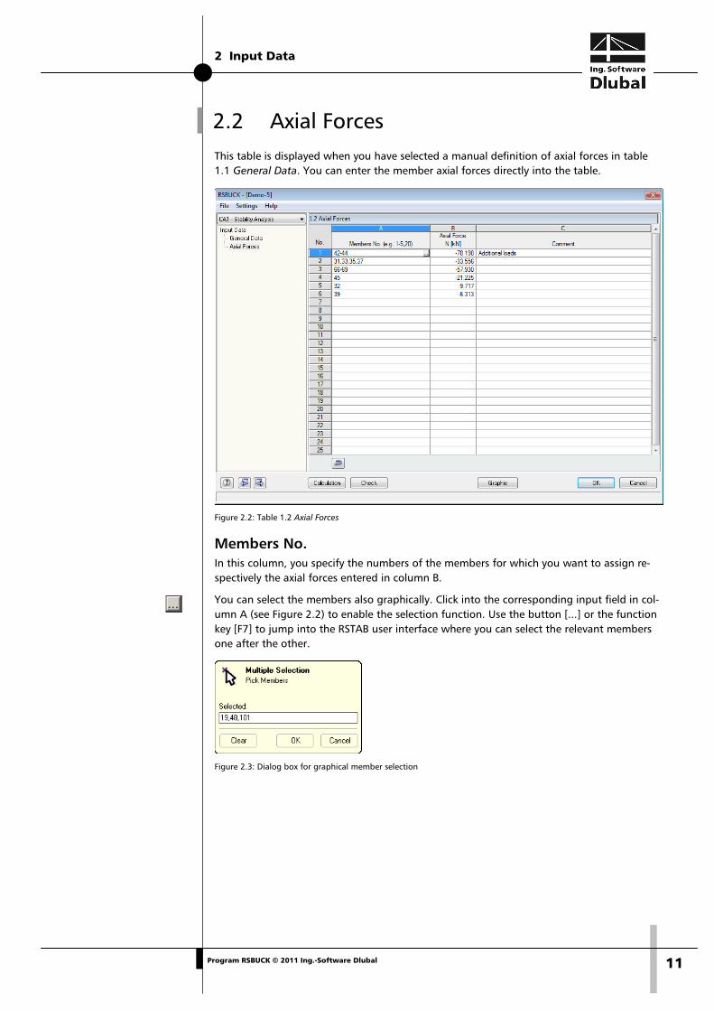
4.2 Buckling Shapes

Figure 4.2: Table 2.2 Buckling Shapes

For each buckling shape the table shows the displacements and rotations of the structure nodes.

4 Results


Node No. The buckling shapes are listed for the structural objects defined in the RSTAB table 1.1 Nodes. Thus, you cannot access any results of member division points in the table.

Shape No. The deformations are displayed for each calculated eigenmode.

Scaled Buckling Shape uX / uY / uZ / ϕX / ϕY / ϕZ The displacements listed in the columns C to E refer to the axes of the global coordinate system and are scaled respectively to the extreme value 1 for each direction.

The columns F to H list the node rotations related to the scaled displacements.

In case the table shows only zero values for the scaled displacements of a member struc-ture, the reason is often to be found in large torsions within the member itself (see figure below). As these effects do not affect the displacements of the member ends, the given buckling lengths and critical loads are of little relevance for these members.

Figure 4.3: Torsion of a thin-walled rectangular column

4 Results


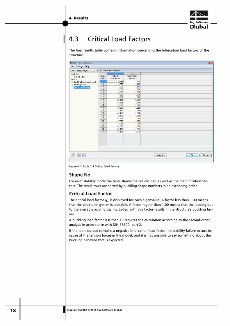
4.3 Critical Load Factors The final results table contains information concerning the bifurcation load factors of the structure.

Figure 4.4: Table 2.3 Critical Load Factors

Shape No. For each stability mode the table shows the critical load as well as the magnification fac-tors. The result rows are sorted by buckling shape numbers in an ascending order.

Critical Load Factor The critical load factor ηcr is displayed for each eigenvalue. A factor less than 1.00 means that the structural system is unstable. A factor higher than 1.00 means that the loading due to the available axial forces multiplied with this factor results in the structure's buckling fail-ure.

A buckling load factor less than 10 requires the calculation according to the second-order analysis in accordance with DIN 18800, part 2.

If the table output contains a negative bifurcation load factor, no stability failure occurs be-cause of the tension forces in the model, and it is not possible to say something about the buckling behavior that is expected.

4 Results


Magnification Factor The magnification factor α is determined according to the following equation:

cr

11

1

η−

=α

Equation 4.2: Magnification factor

The magnification factor gives us information about the relation between the moments ac-cording to the linear-static and the second-order analysis.

III MM ⋅α=

where MI Moment according to linear static analysis, but considering the equiva-lent load for the deformation

MII Moment according to second-order analysis

Equation 4.3: Relation of moments

This equation is only valid in case the bending line under the loading is similar to the buck-ling shape, and if ηcr is higher than 1.00.

5 Results Evaluation


5. Results Evaluation When the stability analysis is complete, several options for results evaluation are available. Moreover, you can use the RSTAB work window to evaluate the results graphically.

5.1 Results Tables First you should have a look at the buckling load factors displayed in table 2.3 Critical Load Factors.

A negative critical load factor indicates that no buckling failure could have been detected because of the axial tension forces. We can interpret this fact in such a way that a buckling failure would arise when the loading's direction of action (inverse signs) is reverse. If neces-sary, a remedy can be found by increasing the determined buckling shapes.

Critical load factors less than 1.00, however, are an indicator for the system's instability.

Figure 5.1: Unstable structural system

Only a positive buckling load factor that is higher than 1.00 permits to say that the loading due to the given axial forces, multiplied with this factor, leads to the buckling failure of the stable structural system.

In table 2.1, different buckling length coefficients K appear per buckling shape for the members.

Figure 5.2: Buckling length coefficients K

During the analysis, the program increases the axial forces iteratively until the critical load case occurs. The critical load is determined from this critical load factor. In turn, the critical load enables conclusions regarding the buckling lengths and buckling length coefficients.

For example, if you want to show the governing buckling length coefficient Ky for the def-lection perpendicular to the "strong" member axis y, you normally have to calculate several buckling shapes. Only for square cross-sections you get the same buckling lengths and buckling length coefficients.

The buckling length coefficients for continuous members cannot be determined directly with the RSBUCK add-on module. It is only possible to evaluate the results of the individual members. The member with the lowest buckling load Ncr displayed in the output can be considered as governing for the entire set of members. Then the K values can be deter-mined from the buckling length of this member and the total length of the set of members.



5.2 Results Graphic The possibility to represent the various buckling shapes graphically helps you to value the stability behavior of the structural system. To evaluate the analysis results graphically, use the RSTAB work window. Click the [Graphic] button to quit the RSBUCK module. The buck-ling shapes are displayed graphically in the RSTAB work window like the deformations of a load case.

The current RSBUCK case is preset. The display shows a changed Results navigator.

Figure 5.3: Results navigator for RSBUCK

The Deformations of all buckling shapes are available as graphical results. It is possible to display specifically every global portion of displacement or rotation.

To turn the display of buckling shapes on or off, use the button [Results on/off] shown on the left.

As the RSTAB tables are of no relevance for the evaluation of RSBUCK results, you may deac-tivate them.

Like the navigator the control panel is aligned with the add-on module RSBUCK. The panel's default functions are described in detail in the RSTAB manual, chapter 4.4.6, page 67. The first tab with the color spectrum appears when the members' deformations are represented with the display option Cross-sections Colored (see Figure 5.6, page 23).



Figure 5.4: Panel for RSBUCK

In the Factors tab of the panel, you can select the buckling shapes.

Figure 5.5: Selection of buckling shapes in the Factors tab

In complex structural systems, it is often difficult to detect buckling members immediately. To facilitate the detection, you can increase the deformation's Display Factors in the Factors tab. The animation of deformations represents another help function that can be activated by means of the button shown on the left.

The display of member results is set in the Results navigator under Results → Deformation → Members. By default, buckling shapes are shown as single-colored Lines. The two re-maining options can also be used to represent the buckling behavior.



Figure 5.6: Display navigator: Results → Deformation → Members → Cross-sections Colored

All graphics can be transferred like RSTAB graphics to the printout report (see chapter 6.2, page 26).

It is always possible to return to the RSBUCK add-on module by clicking the button [RSBUCK] in the panel.

5.3 Filter for Results In addition to the RSBUCK results tables which already allow for a particular selection ac-cording to certain criteria because of their structure, you can use the filter options described in the RSTAB manual to evaluate the RSBUCK analysis results graphically.

On the one hand, you can take advantage of already defined partial views (see RSTAB ma-nual, chapter 9.8.6, page 209) used to group objects appropriately.

On the other hand, you can use the scaled deformations in the RSTAB workspace as filter criteria. The filter settings for results defined in the Color Spectrum tab of the control panel are described in the RSTAB manual, chapter 4.4.6, page 67.

If you use a colored results display, you can use the panel to define for example that only scaled deformations larger than 0.55 are displayed, which may facilitate the detection of members with a risk for buckling in huge models.

Filtering members In the Filter tab of the control panel, you can specify the numbers of the members whose deformations should be shown exclusively in the graphic. A description of this function can be found in the RSTAB manual, chapter 9.8.6, page 209.

Unlike the partial view function, the structure is now displayed completely in the graphic.



5.4 Non-linear RSTAB Calculation Also RSTAB provides the possibility to determine the critical load factor of a load case or a load group. You find the corresponding setting in the Calculation Parameters tab of the di-alog box Edit Load Case - General Data.

Figure 5.7: Dialog box Edit Load Case, option Calculate Critical Load Factor

Click the button [Settings for Analysis of Critical Load Factor] to open another dialog box managing the parameters for the calculation of the buckling load factor. It is recommended to define the Start Load Factor by a value that is not too high in order to ensure that also the first eigenmode is determined.

The determination of the critical load factor according to the second-order analysis is per-formed necessarily according to a non-linear method of calculation. Instead of a linear ei-genvalue analysis, the loading is gradually increased during the determination process. When a particular load increment is reached, the structural system becomes unstable. Thus, the critical load factor is found and shown in the RSTAB table 3.0 Summary together with the origin of instability and the number of iterations.

Figure 5.8: RSTAB table 3.0 Summary

The advantage of this procedure is that all non-linear elements (failing members, supports etc.) can be accurately taken into account when the critical load factor is determined. How-ever, with this approach you can only find the lowest stability mode. Furthermore, the computing time is often higher than the time needed for a linear analysis.

6 Printout


Hence, with regard to the RSBUCK results, minor deviations cannot be excluded in any case because of the different calculation theories.

In case the critical load factor calculated according to the second-order analysis deviates significantly from the RSBUCK analysis, it is recommended to check first of all whether the calculation parameters, which are

• the favorable effect due to tension forces and

• the reduction of stiffness by partial safety factor γM,

have been taken into account in the same way in both cases.

6. Printout

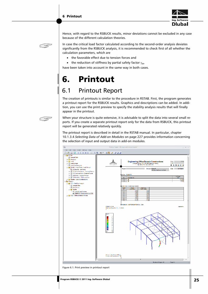
6.1 Printout Report The creation of printouts is similar to the procedure in RSTAB. First, the program generates a printout report for the RSBUCK results. Graphics and descriptions can be added. In addi-tion, you can use the print preview to specify the stability analysis results that will finally appear in the printout.

When your structure is quite extensive, it is advisable to split the data into several small re-ports. If you create a separate printout report only for the data from RSBUCK, this printout report will be generated relatively quickly.

The printout report is described in detail in the RSTAB manual. In particular, chapter 10.1.3.4 Selecting Data of Add-on Modules on page 227 provides information concerning the selection of input and output data in add-on modules.

Figure 6.1: Print preview in printout report

6 Printout


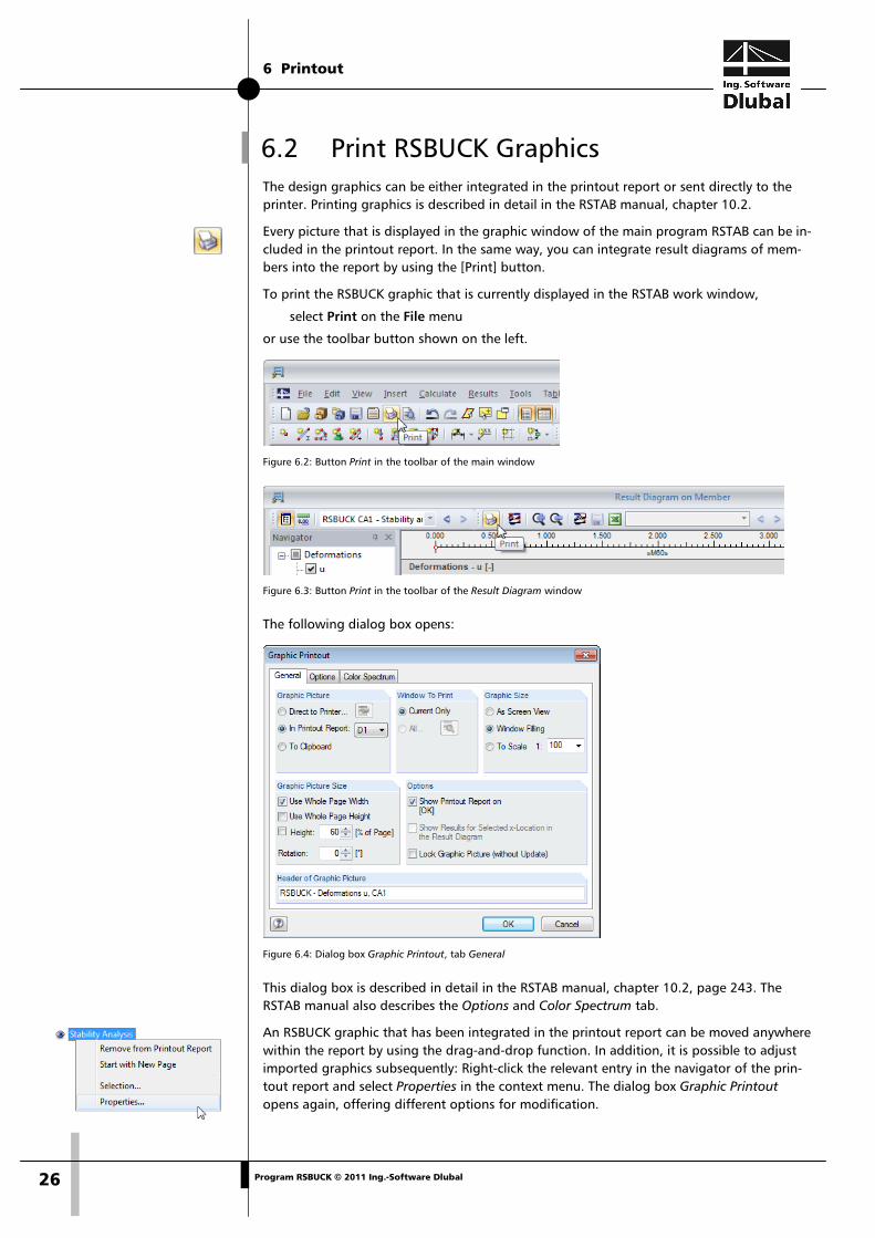
6.2 Print RSBUCK Graphics The design graphics can be either integrated in the printout report or sent directly to the printer. Printing graphics is described in detail in the RSTAB manual, chapter 10.2.

Every picture that is displayed in the graphic window of the main program RSTAB can be in-cluded in the printout report. In the same way, you can integrate result diagrams of mem-bers into the report by using the [Print] button.

To print the RSBUCK graphic that is currently displayed in the RSTAB work window,

select Print on the File menu

or use the toolbar button shown on the left.

Figure 6.2: Button Print in the toolbar of the main window

Figure 6.3: Button Print in the toolbar of the Result Diagram window

The following dialog box opens:

Figure 6.4: Dialog box Graphic Printout, tab General

This dialog box is described in detail in the RSTAB manual, chapter 10.2, page 243. The RSTAB manual also describes the Options and Color Spectrum tab.

An RSBUCK graphic that has been integrated in the printout report can be moved anywhere within the report by using the drag-and-drop function. In addition, it is possible to adjust imported graphics subsequently: Right-click the relevant entry in the navigator of the prin-tout report and select Properties in the context menu. The dialog box Graphic Printout opens again, offering different options for modification.

7 General Functions


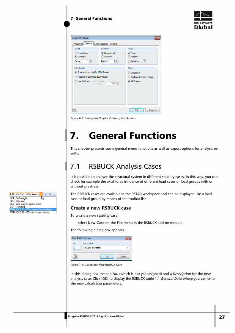
Figure 6.5: Dialog box Graphic Printout, tab Options

7. General Functions This chapter presents some general menu functions as well as export options for analysis re-sults.

7.1 RSBUCK Analysis Cases It is possible to analyze the structural system in different stability cases. In this way, you can check for example the axial force influence of different load cases or load groups with or without prestress.

The RSBUCK cases are available in the RSTAB workspace and can be displayed like a load case or load group by means of the toolbar list.

Create a new RSBUCK case To create a new stability case,

select New Case on the File menu in the RSBUCK add-on module.

The following dialog box appears.

Figure 7.1: Dialog box New RSBUCK-Case

In this dialog box, enter a No. (which is not yet assigned) and a Description for the new analysis case. Click [OK] to display the RSBUCK table 1.1 General Data where you can enter the new calculation parameters.

7 General Functions


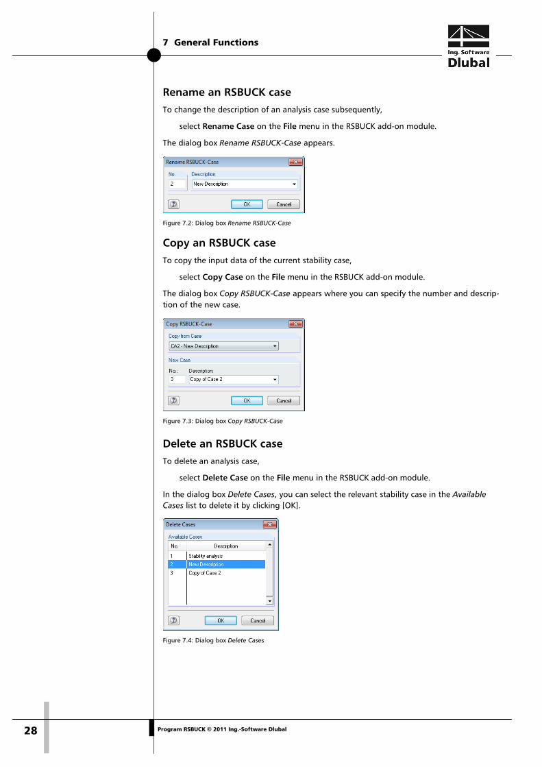
Rename an RSBUCK case To change the description of an analysis case subsequently,

select Rename Case on the File menu in the RSBUCK add-on module.

The dialog box Rename RSBUCK-Case appears.

Figure 7.2: Dialog box Rename RSBUCK-Case

Copy an RSBUCK case To copy the input data of the current stability case,

select Copy Case on the File menu in the RSBUCK add-on module.

The dialog box Copy RSBUCK-Case appears where you can specify the number and descrip-tion of the new case.

Figure 7.3: Dialog box Copy RSBUCK-Case

Delete an RSBUCK case To delete an analysis case,

select Delete Case on the File menu in the RSBUCK add-on module.

In the dialog box Delete Cases, you can select the relevant stability case in the Available Cases list to delete it by clicking [OK].

Figure 7.4: Dialog box Delete Cases

7 General Functions


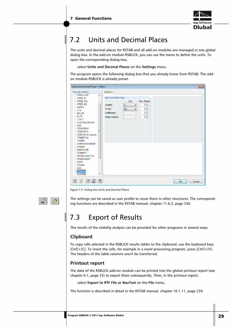
7.2 Units and Decimal Places The units and decimal places for RSTAB and all add-on modules are managed in one global dialog box. In the add-on module RSBUCK, you can use the menu to define the units. To open the corresponding dialog box,

select Units and Decimal Places on the Settings menu.

The program opens the following dialog box that you already know from RSTAB. The add-on module RSBUCK is already preset.

Figure 7.5: Dialog box Units and Decimal Places

The settings can be saved as user profile to reuse them in other structures. The correspond-ing functions are described in the RSTAB manual, chapter 11.6.2, page 336.

7.3 Export of Results The results of the stability analysis can be provided for other programs in several ways.

Clipboard To copy cells selected in the RSBUCK results tables to the clipboard, use the keyboard keys [Ctrl]+[C]. To insert the cells, for example in a word processing program, press [Ctrl]+[V]. The headers of the table columns won't be transferred.

Printout report The data of the RSBUCK add-on module can be printed into the global printout report (see chapter 6.1, page 25) to export them subsequently. Then, in the printout report,

select Export to RTF File or BauText on the File menu.

The function is described in detail in the RSTAB manual, chapter 10.1.11, page 239.

7 General Functions


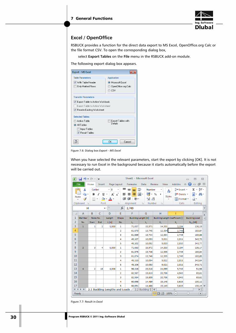
Excel / OpenOffice RSBUCK provides a function for the direct data export to MS Excel, OpenOffice.org Calc or the file format CSV. To open the corresponding dialog box,

select Export Tables on the File menu in the RSBUCK add-on module.

The following export dialog box appears.

Figure 7.6: Dialog box Export - MS Excel

When you have selected the relevant parameters, start the export by clicking [OK]. It is not necessary to run Excel in the background because it starts automatically before the export will be carried out.

Figure 7.7: Result in Excel

7 General Functions


RSIMP If you want to use a stability mode in the add-on module RSIMP to generate equivalent im-perfections or a pre-deformed initial structure, you do not need to export the data. RSIMP enables you to select the relevant buckling shape No. as well as the RSBUCK Case directly in the corresponding lists.

Figure 7.8: Selection of buckling shape and RSBUCK case in the add-on module RSIMP

KAPPA / TIMBER Pro The add-on modules KAPPA and TIMBER Pro provide the option to apply the buckling length coefficients from RSBUCK directly for the members that you want to design.

Figure 7.9: Selection of buckling length coefficient in the add-on module KAPPA

8 Examples


8. Examples

8.1 Euler Buckling Mode 1 The critical load of a restrained column must be determined. The model, due to its type of loading and support conditions, corresponds to the Euler buckling mode 1.

10,0

0 m

N

Figure 8.1: Model for Euler buckling mode 1

Analytical solution The lowest critical load Ncr is determined according to the following equation:

2

2

crL

IEN

π⋅⋅=

Equation 8.1

The cross-section, defined as rolled cross-section HE-B 300, has the following second mo-ments of area:

Iy = 25170 cm4

Iz = 8560 cm4

Steel S235 is used as material.

E = 21000 kN/cm2

For a column that is restrained only at one end (Euler buckling mode 1) the buckling length coefficient K = 2 is applied.

The buckling load for the deflection perpendicular to the z-axis is determined as follows:

kN54.443)10002(

856021000N

2

2

cr =⋅

π⋅⋅=

8 Examples


Solution with RSTAB The column is modeled as a 3D structure.

Figure 8.2: RSTAB model and loading

The loading is represented by a concentrated load of 100 kN applied to the top column node. The automatic self-weight is deactivated for the general data of the load case.

The RSBUCK input table is filled in as follows:

Figure 8.3: RSBUCK table 1.1 General Data

8 Examples


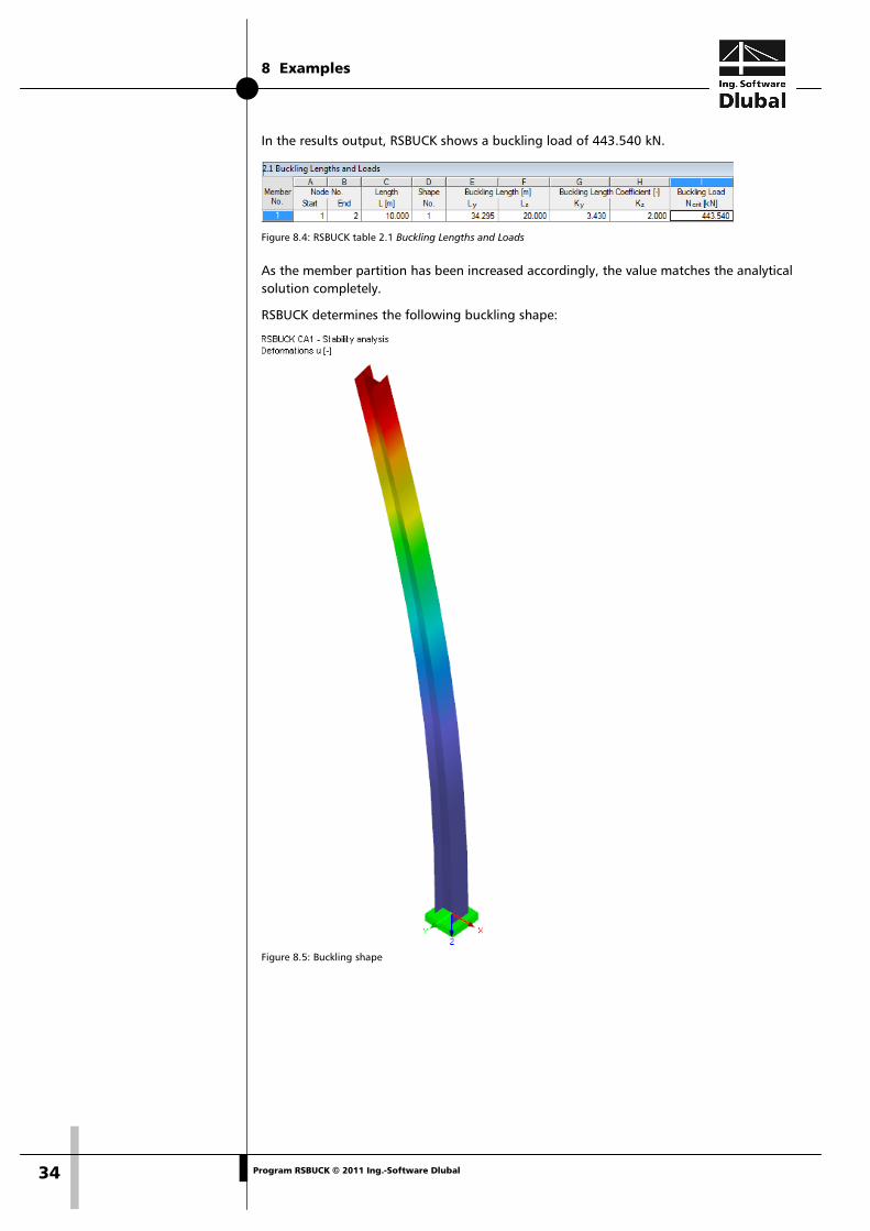
In the results output, RSBUCK shows a buckling load of 443.540 kN.

Figure 8.4: RSBUCK table 2.1 Buckling Lengths and Loads

As the member partition has been increased accordingly, the value matches the analytical solution completely.

RSBUCK determines the following buckling shape:

Figure 8.5: Buckling shape

8 Examples


8.2 Frame with K-Bracing Based on the 2D model shown in the figure below, we want to determine the buckling length coefficients of the structure's frame posts. The example is taken from [1], page 395.

Figure 8.6: Analysis model for steel frame

Analytical solution The analytical solution is presented in [1], example 5.47. We assume to have a ratio of com-pression forces in the posts that is D2/D1 = 0.8, this means the axial force in member 2 is 80 % of the axial force available in member 1.

For our planar structural system, the following buckling length coefficients are determined in [1]:

Member Buckling length coeffi-cient K

1 2.73

2 3.07

Table 8.1: Buckling length coefficients according to [1], page 397

Solution with RSTAB A 2D system is created and the members are defined with the corresponding HE-B cross-sections. The posts are defined as member type Beam, the horizontal and diagonal beams are defined as Truss (only N).

Both support nodes are supported by hinged supports.

To get the axial force distribution in the posts that we want, the two topmost post nodes are each stressed by a concentrated load of 100 kN. Further concentrated loads of 25 kN are applied in the post centers to the connection nodes of the diagonals. The automatic self-weight is not taken into account.

8 Examples


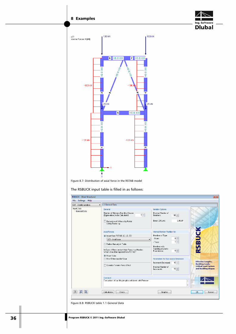
Figure 8.7: Distribution of axial force in the RSTAB model

The RSBUCK input table is filled in as follows:

Figure 8.8: RSBUCK table 1.1 General Data

8 Examples


In the results output RSBUCK shows the following buckling length coefficients K:


Thus, the results are matching the analytical solution very well.

RSBUCK determines the following buckling shape:

Figure 8.10: Buckling shape

8 Examples


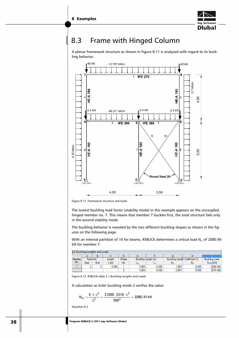
8.3 Frame with Hinged Column A planar framework structure as shown in Figure 8.11 is analyzed with regard to its buck-ling behavior.

Figure 8.11: Framework structure and loads

The lowest buckling load factor (stability mode) in this example appears on the uncoupled, hinged member no. 7. This means that member 7 buckles first, the total structure fails only in the second stability mode.

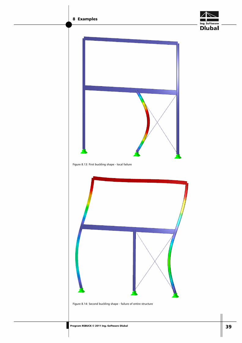
The buckling behavior is revealed by the two different buckling shapes as shown in the fig-ures on the following page.

With an internal partition of 10 for beams, RSBUCK determines a critical load Ncr of 2080.94 kN for member 7.


A calculation as Euler buckling mode 2 verifies the value:

kN91.2080500

251021000

L

IEN

2

2

2

2

cr =π⋅⋅

=π⋅⋅

=

Equation 8.2

8 Examples


Figure 8.13: First buckling shape - local failure

Figure 8.14: Second buckling shape - failure of entire structure

A Literature


A Literature

[1] PETERSEN, Chr.: Statik und Stabilität der Baukonstruktionen, Vieweg & Sohn Verlag, Braunschweig/Wiesbaden, 2. Auflage 1982

[2] PETERSEN, Chr.: Stahlbau, Vieweg & Sohn Verlag, Braunschweig/Wiesbaden, 1988

[3] HÜNERSEN, G.; FRITSCHE, E.: Stahlbau in Beispielen - Berechnungspraxis nach DIN 18800 Teil 1 bis Teil 3, Werner Verlag, Düsseldorf, 4. Auflage 1998

[4] RUBIN, H; SCHNEIDER, K.-J.: Baustatik - Theorie I. und II. Ordnung, Werner Verlag, Düsseldorf, 3. Auflage 1996

[5] OWCZARZAK, H; STRACKE, M.: Seminarunterlagen zum Dortmunder Praxisseminar - DIN 18800 und EC 3 vom 02.12.94

[6] WERKLE, H.: Finite Elemente in der Baustatik, Vieweg & Sohn Verlag, Wiesbaden, 3. Auflage 2008

B Index


B Index A

Axial force distribution .................................. 9

Axial forces .............................................. 9, 11

B

Break off limit ................................................ 9

Buckling failure ...................................... 18, 20

Buckling length ............................................ 15

Buckling length coefficient K ........... 16, 20, 35

Buckling length L ................................... 15, 16

Buckling load ............................................... 16

Buckling load factor ..................................... 24

Buckling shape ..................... 15, 16, 21, 22, 38

C

Calculation ................................................... 12

Check ........................................................... 12

Cholesky decomposition .............................. 14

Color spectrum ............................................ 23

Comment ............................................... 10, 12

Continuous members .................................. 20

Control panel ............................................... 21

Critical load.................................................. 32

Critical load factor ................................. 18, 20

CSV export ................................................... 30

D

Decimal places ............................................. 29

E

Eigenmode .................................................. 17

Euler buckling modes .................................. 16

Excel ............................................................ 30

Export of results .......................................... 29

F

Filter ............................................................ 23

Flexural buckling load Ncr ............................. 16

G

General data .................................................. 8

Graphic ........................................................ 21

I

Increment .................................................... 10

Instability ..................................................... 20

Installation ..................................................... 5

Iteration options ............................................ 9

Iterations ........................................................ 9

K

KAPPA .......................................................... 31

M

Magnification factor .................................... 19

Member ....................................................... 15

Member length ............................................ 15

Member partition ......................................... 10

Members ...................................................... 11

N

Navigator ....................................................... 8

Non-linear calculation .................................. 24

Number of buckling shapes ........................... 8

O

OpenOffice ................................................... 30

P

Panel .................................................. 7, 21, 23

Partial safety factor γM .............................. 9, 25

Partial view ................................................... 23

Print ............................................................. 26

Print graphic................................................. 26

Printout report ............................................. 25

Q

Quit RSBUCK .................................................. 8

R

Reduction of stiffness ..................................... 9

Result diagrams ............................................ 26

Results evaluation ........................................ 20

Results navigator .................................... 21, 22

Results tables ............................................... 14

RSBUCK case ................................................ 27

RSIMP ........................................................... 31

RSTAB work window .................................... 21

S

Scaled buckling shape .................................. 17

Second-order analysis ...................... 18, 19, 24

Selecting tables .............................................. 8

Stability case .......................................... 27, 28

Start calculation ........................................... 13

B Index


Start program ................................................ 6

Start RSBUCK ................................................. 6

Stiffness ................................................... 9, 25

Sub-space dimension ................................... 10

T

Tables ............................................................ 8

Taper ........................................................... 10

Tension forces .................................. 10, 18, 25

TIMBER Pro ................................................... 31

U

Units ............................................................. 29

User profile................................................... 29

V

Visualization ................................................. 21

Documents

dlubal-tutorial