D.L. Farmer(1), M. Sivapalan(1), and I. Lockley(2)

Assessing vegetation influence on water balance in rehabilitation landscapes using

simple storage models

(1) Centre for Water Research, University of Western Australia, Nedlands, WA 6907(2) Alcoa World Alumina Australia, Applecross, WA 6153

semi- imperv ious base

root zone

daily precipitation

Aug-Sepsemi- imperv ious base

root zone

daily precipitation

Jun-Julsemi- imperv ious base

root zone

daily precipitation

JanJansemi- imperv ious base

root zone

daily precipitation

Mar-Apr

?

* rehab. survival* maximise water ‘interception’* low permeability base, perc = f(H)

* lateral flows (landscape)* resolve management needed

Why ?

* shallow profile 2-4m* residue sand (~homog)* potentially small gradients* water use = f(trees)

Situation...

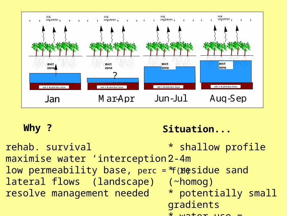
0 5 10 15 20 250

20

40

60

80

100

120

140

160

mm

/ f

ortn

ight

fornight (Feb99-Jan00)

Pinjarra: precipitation vs. evap. potential

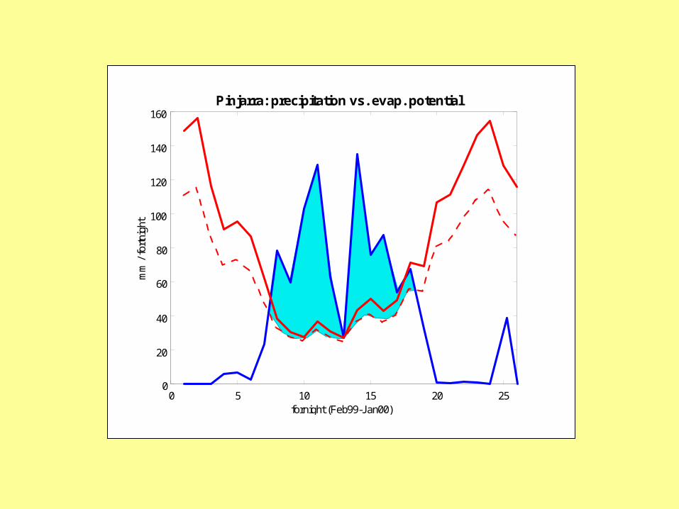
ev apotranspiration (ET)

[root plus WT]

precipitation (P)

uptake by water

plants

percolationwt

root zone

ev apotranspiration (ET)

precipitation (P)

perc

olat

ion

wt

ev apotranspiration (ET)

[root + some WT]

precipitation (P)

some water uptake by

trees

percolationwt

Simple 1D storage based model (dynamic) :

* vegetation: LAI, root depth vegetation ‘grown’ in model

* stores: root , unsat, Hwt store balances computed daily

* fluxes: ET, Qperc, Qwt-root Q = func( fc) [simple threshold approach] Q = suction flow across unsat zone

* recorded data: P, Ep also Irrigation, Qout

lumped water content in 3 zones - root, unsat (root-Hwt), WT

Shallow WT homogenous, permeable sand no lateral flows

ET = ?

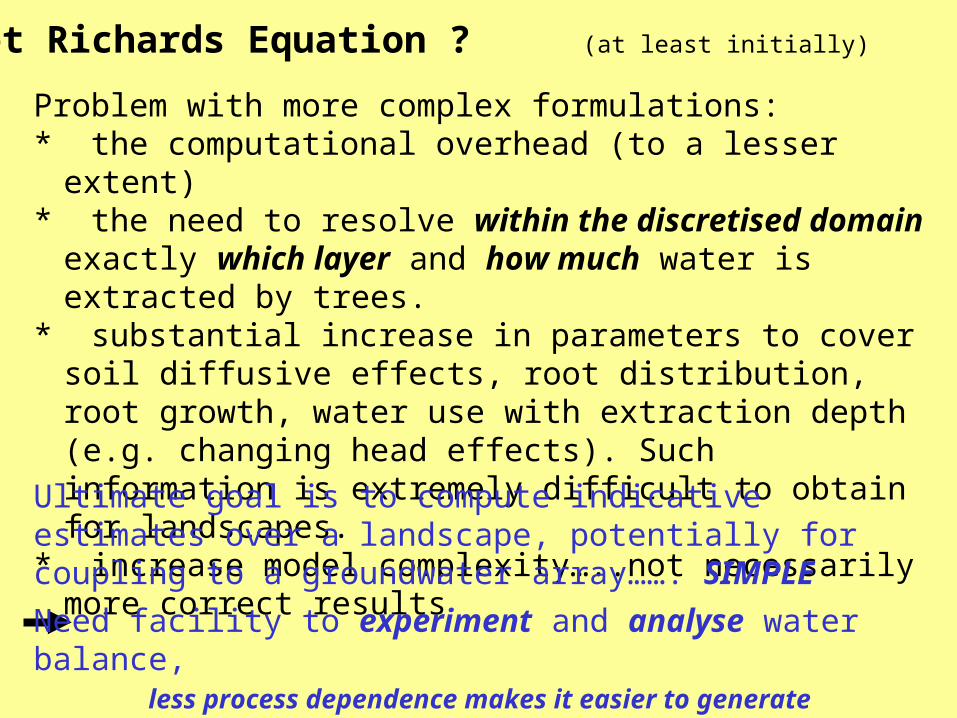
Why not Richards Equation ? (at least initially)

Problem with more complex formulations:* the computational overhead (to a lesser extent) * the need to resolve within the discretised domain exactly which

layer and how much water is extracted by trees. * substantial increase in parameters to cover soil diffusive effects,

root distribution, root growth, water use with extraction depth (e.g. changing head effects). Such information is extremely difficult to obtain for landscapes.

* increase model complexity…..not necessarily more correct results

Ultimate goal is to compute indicative estimates over a landscape, potentially for coupling to a groundwater array……. SIMPLE

Need facility to experiment and analyse water balance, less process dependence makes it easier to generate understanding.

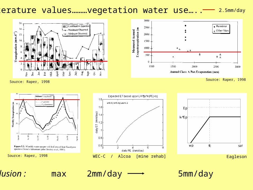
Literature values………vegetation water use…..

Source: Raper, 1998

Source: Raper, 1998

Source: Raper, 1998

fc sat

Ep

kv*Ep

wp

Conclusion : max 2mm/day 5mm/day

2.5mm/day

EaglesonWEC-C / Alcoa [mine rehab]

** details in paper

Water balance model

ET ‘model’idea: to experiment with

various options

* realistically ET = func [biomass (LAI), root depth, root, ‘stresses’]

* ability to set maximum threshold, to explore ‘acceptable’ ET ranges* assumption that trees would grow !! [set by defined t, LAI ]

*

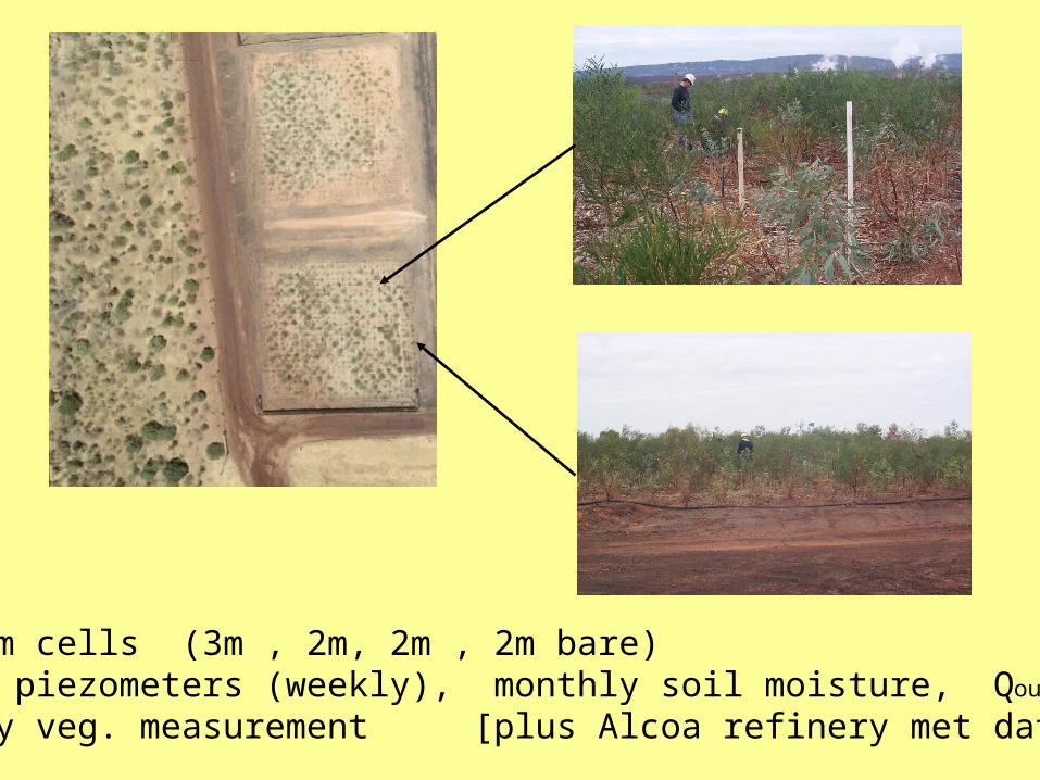
30m x 30m cells (3m , 2m, 2m , 2m bare)multiple piezometers (weekly), monthly soil moisture, Qout, 6 monthly veg. measurement [plus Alcoa refinery met data]

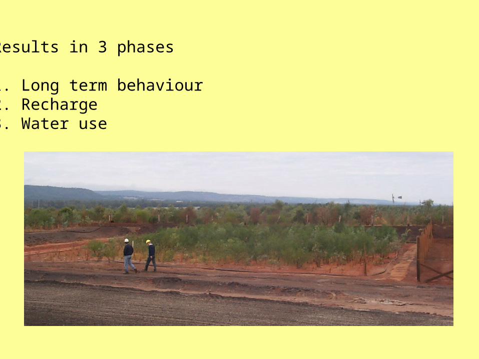
Results in 3 phases

1. Long term behaviour 2. Recharge3. Water use

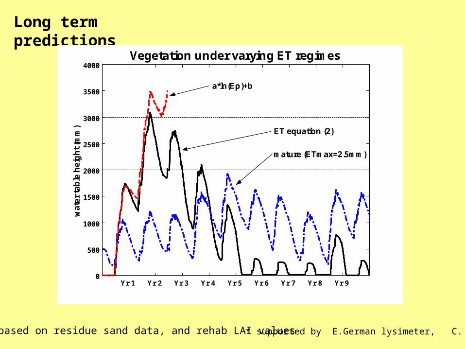
Long term predictions

* supported by E.German lysimeter, C. Hinz

Yr 1 Yr 2 Yr 3 Yr 4 Yr 5 Yr 6 Yr 7 Yr 8 Yr 9 0

500

1000

1500

2000

2500

3000

3500

4000

wa

ter

tab

le h

eig

ht

(mm

)

Vegetation under varying ET regimes

a*ln(Ep)+b

ET equation (2)

mature (ETmax=2.5mm)

* based on residue sand data, and rehab LAI values

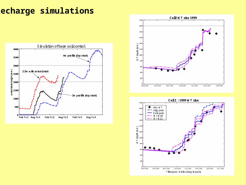
Recharge simulations

Feb Yr 1 Aug Yr 1 Feb Yr 2 Aug Yr 2 Feb Yr 3 Aug Yr 30

500

1000

1500

2000

2500

3000

3500

4000Simulation of bare soil control

wa

ter

tab

le h

eig

ht

(mm

)

4m profile (dry start)

2m profile (dry start)

2.5m with actual start

1MAR1999 1APR1999 1MAY1999 1JUN1999 1JUL1999 1AUG1999 1SEP1999 1OCT19990

200

400

600

800

1000

1200

1400

1600

1800

2000

2200

* first year - minimal veg impacts

WT

de

pth

(m

m)

Cell 1 : 1999 WT rise

obs. WT orig. parsKala pars fc = 0.10 fc = 0.12

1MAR1999 1APR1999 1MAY1999 1JUN1999 1JUL1999 1AUG1999 1SEP19990

200

400

600

800

1000

1200

1400

1600

1800

2000

2200

WT

de

pth

(m

m)

Cell2 WT rise 1999

Water use simulation and episodic recharge…..

1OCT1999 1NOV1999 1DEC1999 1JAN2000 1FEB2000 1MAR20000

200

400

600

800

1000

1200

1400

1600

1800

2000

2200Cell2 storm analysis

* underflow till end OctW

T d

ep

th (

mm

)

1NOV1999 1DEC1999 1JAN2000 1FEB2000 1MAR2000 1APR20000

500

1000

1500

2000

2500

3000

** rainfall bars are mm x10

3m vegetated cell

low LAI 2m cell

M=unlimited evap, red=fc

j m m j s n j m m j s n j m m j s n j m m j s n0

50

100

150

200

250Monthly Precipitation for simulation [Pinjarra]

mm

pe

r m

ont

h

month (Jan yr1 to Dec yr 4)j m m j s n j m m j s n j m m j s n j m m j s n

0

50

100

150

200

250Monthly Excess Water for simulation [Pinjarra]

mm

pe

r m

ont

h

month (Jan yr1 to Dec yr 4)

pre

cip

itatio

n (m

m)

rech

arg

e (

mm

)

Long term excess water prediction…. (provided expected values attained)

Conclusions:* would appear that the simple model is capable of capturing the essence of the

water table behaviour, particularly in discriminating recharge rainfall events (though no long term continuous data as yet).

* evapotranspiration remains an issue, hopefully cells and ongoing work will begin to answer some of these questions. (but expect that >2.5mm based on current data)

* in many situations the water balance of the root zone is more critical than total storage within the system. Simple approach offers means to meaningfully assess potential recharge variability.

Further application: * representation can be even simpler, particularly in ‘mature’ and forested

landscapes. (though extraction ratios between unsat/WT an issue) * capacity to use in catchment water balance models to simply simulate

unsaturated water balance (failing of many hydrology models in SW regions). * sufficiently simple for coupling to shallow aquifer GW models to overcome

‘constant recharge’ and ‘episodic recharge’ issues.* potential to extend idea to ‘hillslope’ models looking at integrated SWM for

indicative analysis (low relief landscapes).

1FEB1999 1MAY1999 1AUG1999 1NOV1999 1FEB2000 1MAY2000 1AUG20000

0.2

0.4

0.6

0.8

1

1.2

1.4

1.6

1.8

2

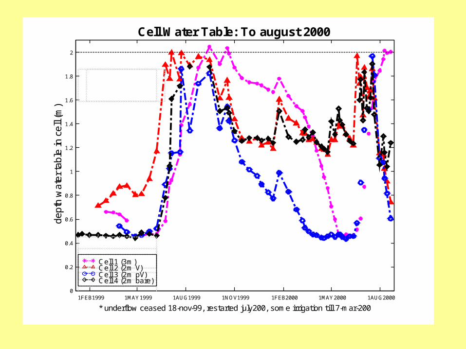
Cell Water Table: To august 2000

de

pth

wa

ter

tab

le in

ce

ll (m

)

* underflow ceased 18-nov-99, restarted july200, some irrigation till 7-mar-200

Cell 1 (3m) Cell 2 (2m V) Cell 3 (2m pV) Cell 4 (2m bare)