Embed Size (px)
Citation preview
Russian Real Wages Before and After 1917: in Global Perspective
Robert C. Allen and Ekaterina Khaustova
May 2017
Working Paper # 0003
Division of Social Science Working Paper Series
New York University Abu Dhabi, Saadiyat Island P.O Box 129188, Abu Dhabi, UAE
http://nyuad.nyu.edu/en/academics/academic-divisions/social-science.html

Russian Real Wages Before and After 1917: in Global Perspective
by
Robert C. Allen
Global Distinguish Professor of Economic HistoryFaculty of Social Science
New York University Abu [email protected]
Ekaterina Khaustova
Russian State Social [email protected]
2017
We thank New York University Abu Dhabi and the Russian Presidential Academy ofNational Economy and Public Administration for research support.

Russian Real Wages Before and After 1917
The working class is the protagonist of the Russian Revolution. In Marxist accounts,the exploitation of the proletariat increased as the Russian economy expanded before the FirstWorld War, and that increasing exploitation was the major background factor leading to theoverthrow of Russian capitalism. Is there, in fact, evidence that real wages declined or thatexploitation in any other sense increased prior to 1913? There have been surprisingly fewattempts to measure changes in real wages in this period1. As socialism developed after1917, capitalist exploitation, presumably, ended, so the standard of living of workers shouldhave risen. But did it? What happened to the standard of living of Russian workers after1917? There is even less research on this topic.2 A substantial literature has found that livingstandards fell after 19283, but what about the years of the NEP? This paper uses newlyassembled data bases to answer these questions.
An unusual feature of our investigation is that we consider Russian wage history froman international perspective. In recent years, many scholars have measured real wages andused them as an indicator of economic growth for a growing list of countries over a longerand longer time frame.4 One country notably missing from the list is Russia, and it is the aimof this paper to fill that gap. This is important for several reasons. First, Russia is the largestcountry in Europe. The history of the continent can never be complete without studyingRussia. Second, more particularly, in Gerschenkron’s (1962) influential schema ofindustrialization in Europe, Tsarist Russia was the archetypical backward country. In themiddle of the nineteenth century, its huge agrarian sector and feudal social system placedRussia hundreds of years behind western Europe in social and economic development. Gerschenkron thought that this situation meant that Russia’s institutions and growthexperience were markedly different from those of Britain, the archetypical advanced country,and Germany, the intermediate country. Did Russia also have a unique history of realwages? Third, while Gerschenkron was not so sure that his schema extended to othercontinents, we must wonder how Europe’s ‘backward’ country compared to other ‘backward’countries like India, Japan, and Egypt. Were real wages higher in Russia than wages inleading countries in Asia and Africa or were they at a similarly miserable level? Dideconomic growth translate into rising real wages in any of these economies?
1Mironov (2010) is the most recent. See also Allen (2003, pp. 37-46) and Borodkin,Grenville, and Leonard (2008).. Gregory (1980) studies the growth of consumption per head,which covers the whole society and not just workers.
2Most research is concerned with either what happened before the First World War orwhat happened after the start of the Five Year Plans in 1928. Zaleski (1971, p. 390) did linkreal wage indices to span the period 1900-1927/8 but never discussed the results!
3Chapman (1954, 1963), Bergson (1961), Hunter and Szyrmer (1992). Allen (2003)reaches more optimistic conclusions.
4Allen (1994, 2001, 2007), Allen, Murphy, and Schneider (2012), Allen, Bassino, Ma,Moll-Murata, and van Zanden (2011), Arroyo Abad, Davies, van Zanden, (2012), Bassinoand Ma (2006), Broadberry and Gupta (2006), Broadberry, Campbell, Klein, Overton, vanLeeuwen (2015), Frankema and van Waijenburg (2012), Özmucur and Pamuk (2002), Pamukand Shatzmiller (2104), Plessis and Plessis (2012), Rönnbäck (2014)., Schneider (2013), VanZanden (1999), Zwart (2016), Zwart and van Zanden (2015).

2
The international comparisons we consider turn out to be important for anotherreason, as well, namely they change our understanding of Russian history. Once the data areassembled, it is straight forward to calculate the change in real wages realized by workers incotton mills in Russia between 1913 and 1928, for instance, but what we make of that changedepends very much on our perspective. From a Russian point of view, the change looks quitelarge; from a global perspective, it is not so great. International comparisons show usRussian history in a new light, as we will see.
Data sources
Our investigation is based on a wide ranging collection of new data for the Imperialperiod and the NEP. (For the extension to 1937, we saw no need to add to the comprehensivecollection of information by Zaleski (1955) and Chapman (1963)). The data include wagerates and the prices of consumer goods.5 While previous work like Mironov’s hasconcentrated on St. Petersburg, we collected data for Moscow and Kursk as well as thecapital. Mironov collected new data for St Petersburg for 1703-1853 but relied on anoutmoded Soviet index to measure inflation between 1853 and 1913. We have collectedoriginal data for St. Petersburg to compute a better weighted index for that period. Moscowand St. Petersburg were the two largest industrial centres, so it was essential to include bothof them in view of our focus on the industrial proletariat. We added Kursk precisely becauseit was a small, provincial manufacturing city. While we do not claim that it represents all ofRussia outside of the two leading cities, we do think it is a weather vane that may indicatetrends in outlying districts that warrant further study.
Our information for Moscow and St Petersburg before the First World War camelargely from municipal statistical handbooks: Vedomosti spravochnich tsen v SaintPetersburge na pripasi, materiali, platy rabochim i prochee, izdavaemie Saint Petersburggorodskoi ypravoi. (Saint Petersburg 1854-1917) and Vedomosti o spravochnix tsenax napripasi I materialy v Moskve (Moscow 1871-1917), Ezemesyachniy statisticheskii bylleten pogorody Moskve (1892-1917). The 1899 volume for St. Petersburg and the 1883 volume forMoscow were missing from the collection in the Russian National Library, so we interpolatedthe gaps.
These sources include monthly and sometimes weekly data. We collected monthlydata for bread and for the wages of carpenters and labourers. For other items, we collectedquarterly data. The data were then averaged to create annual series that were representativeof conditions throughout the year.
The Moscow yearbooks began in 1871. For earlier years, we collected prices andwages from Tsentralniy Gosydarstvenniy Arxiv Goroda Moskvi. The major data source was Raporti torgovix starost o tsenax, Spravochnie tseni vedomstva Moskovskoi dvottsovoi konoria tak ze ministerstva Imperatorskogo Dvora, O dostavlenii spravochnix tsen i materialov,Delo Moskovskoi rasporiaditelnoi dymi o dostavlenii spravochnix tsen, Delo Moskovskoigorodskoi dymi. With this information, we could trace the same types and qualities of goodsand labour back to the 1820s.
There were no statistical yearbooks for Kursk, so all information was obtained fromrecords in the archive Gosydarstvenniy Arkhiv Kyrskoi Oblasti.
To study wages and at the height of the New Economic Policy, we collected data for
5Full references to the data are listed in the Appendix.

3
1924-9. Our main source was Ezemesyachnii statisticheskii bylleten po gorody Moskve IMoskovskoi Gybernii where we found prices for many goods sold in state and cooperativeshops and on the private market. We calculated a weighted average price where the weightsreflected sales in 1928.6 The prices of bread, beef, and potatoes were affected, for the privatemarket accounted for 5%, 11%, and 76% of the sales of these foods.
The history of nominal wages
We have collected data for three types of workers–building craftsmen (carpenters,bricklayer, or masons), building labourers, and employees in cotton textile mills. Buildingcraftsmen and labourers figure in virtually all studies of historical real wages since everycountry had a construction industry, and building workers were hired by the institutionswhose records are the main source of historical wages and prices (Beveridge 1939, pp. xxi-xxvi, xlix-lii). While payment in building was often purely monetary–where it was not thevalue of payments in kind must be added to the cash component–there is a question of howcontinuously the workers were employed. In our comparisons, we assumed they worked afull year, which may not have been true.7 To judge the seriousness of this issue, we alsodiscuss the average earnings of workers in cotton mills. Many countries had cotton mills bythe late nineteenth century, cotton was the exemplar of the new industrial order, and the millsoperated throughout the year, so the seasonality issue that is present in construction does notarise.
We have collected data on building wages for Moscow, St. Petersburg, and Kursk. The former two were the major industrial cities of Russia, while Kursk was a provincialcentre included to test the generality of the patterns observed for Moscow and St. Petersburg. We compare these wages to those in four other countries–the two leading economies of theperiod (the UK and the USA) and two less developed countries (India and Egypt). For theUK we focus on Manchester, although wages for London have also been examined, and theirhistory is similar. For the USA, we concentrate on Boston. In the case of both of thesecountries, labour markets became increasingly integrated, so that by the twentieth century,both real and nominal wage levels were similar in all of the major industrial centres. In thecases of India and Egypt we focus on Bombay and Cairo.
Our wages for cotton mill workers are national averages. It will be noted that thecities whose building wages we study were also centres of cotton textile production. Thisimproves comparability between the different types of wages. Also, our cost of living indicespertain to the cities for which we have building wages. Since these are also cotton textilecentres, the price indices should be appropriate for cotton as well.
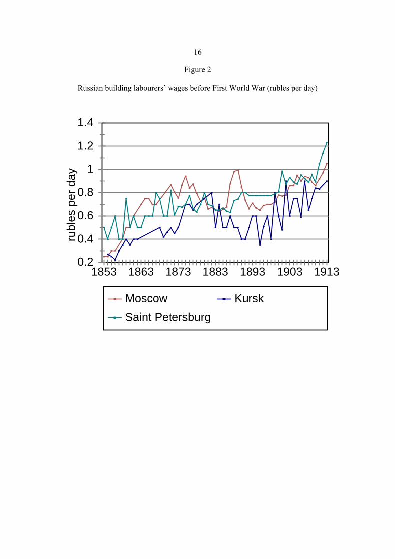
We begin with building wages for Russian cities. Figure 1 plots the daily wage ofcarpenters, and Figure 2 shows the wages of labourers. The earnings of labourers weresimilar in all three cities. The earnings of carpenters were higher. Carpenters in Moscow andSt Petersburg were similar. The wages of carpenters in Kursk were on a par with those inMoscow before about 1860 and slid significantly behind in the late nineteenth century when
6“Comparison of Real Wages in Various Cities,” International Labour Review, 1928,pp. 659.
7When our sources give monthly wage rates, they report rates for every month, butthey do not indicate employment levels by month.

4
they were little above the earnings of labourers. Kursk were not keeping up with wages innthe big cities in this period. The similarity of wages in Moscow and St Petersburg raises thepossibility that their labour markets were integrated, while the lower carpenter’s wages inKursk suggests that integration did not extend to all cities.
How did Russian wages compare to those in other countries? Figures 3 and 4compare the wages of building craftsmen and labourers in leading cities before the FirstWorld War. All wages have been converted to US dollars at the prevailing exchange rates. The pattern of earnings is the same for both skill levels. Earnings were always higher inManchester and Boston than in other cities, with USA in the lead and pulling increasinglyahead of Britain in the decade before the First World War. Egypt and India were at thebottom of the League Table. Moscow and St Petersburg were closer to Bombay and Cairothan they were to Boston and Manchester.
Industrialization is about the growth in manufacturing as well as construction, so wealso consider earnings in industry. Data are available of average earnings in themanufacturing sector. Since earnings varied considerable among industries in all countriesand since the mix of industries differed between countries, we focus on one industry, namely,cotton textiles. It was often the first sector in which factory production took off, and itemployed a similar workforce with many women and children in most countries.8 Thismakes comparisons more meaningful.
Figure 5 shows the average annual earnings of employees in cotton mills in the USA,UK, Russia, and India before the First World War. The pattern is similar to the pattern forbuilding workers: Annual earnings were highest in the USA followed by Great Britain. Indian earnings were lowest. Russian earnings were about double Indian earnings but onlyhalf of those in the UK and one third of the US level. We have no time series data for Egyptsince its industry was so small, but the scattered information indicates that earnings werebetween those in Russia and India (Allen 2015).
If we extend these wage series to the Second World War, many features remain thesame although there are expected alterations (Figures 6-8). The USA and Britain remain thehighest paying countries. The wage stagnation that appeared in late nineteenth centuryBritain continues, and the USA lead over the UK becomes much greater after the First WorldWar. The 1920s were difficult for Britain, while the USA boomed. Indian and Egyptianwages remained very low.
The most dramatic change by far was in Russian wages. These increased quitedramatically after 1917. By the late 1930s, the earnings of Russian building labourers andcraftsmen were approaching USA levels when Russian rubles are converted to USA dollars. The earnings of Russian cotton mill workers surged ahead of American earnings. It is truethat nominal earnings inflated considerably in Russia, especially after 1928. However, muchof the rise in Russian earnings when converted to dollars reflects exchange rate policy. Wecan only see whether the increase represents an improvement in real purchasing power if werelate the Russian earnings to Russian consumer goods prices expressed in the samecurrency.
the cost of subsistence
8The Indian industry is an exception to this generalization, for in India most cottonmill workers were adult men.

5
Comparisons of nominal wages show dramatic differences between countries with thehighest nominal wages being in the richest countries. To the degree that countries were opento world trade, one might expect that differences in nominal earnings would have translatedinto differences in real earnings since international trade tends to equalize the prices ofinternationally traded goods like food, cloth, etc. Countries, however, differed considerablyin their openness to trade. The UK practised complete free trade until the depression of the1930s and forced India and Egypt to have very low tariffs. On the other hand, the USA andRussia pre-1917 had very high protective tariffs on manufactured goods, but no tariffs on theagricultural products which they exported. While international trade might have equalizedtheir agricultural prices, it would not have equalized cotton cloth prices, for instance. Evenin the case of the UK, some goods (eg housing) were not traded, so trade would not equalizetheir cost. And, of course, the Soviet Union in the 1930s was about as far from free trade asit was possible for a country to be, so expectations based on international arbitrage areirrelevant to its circumstances. The only way to find out what wages could buy is to calculatethe cost of living.
Our approach to measuring the standard of living is an extension of the establishedprocedure based on subsistence baskets and welfare ratios. The welfare ratio equals theannual earnings of the worker concerned divided by the cost of maintaining a family atsubsistence (Blackorby and Donaldson 1987, Allen 2001). If the welfare ratio equals one,then the worker earns just enough to keep his family at subsistence. If the ratio is less thanone, then earnings are inadequate even for that low standard and either painful decreases inspending are required or more income has to be generated by increasing the family’s scale ofpaid work. If the ratio exceeds one, then there is a surplus over subsistence. This is oftenrealised by increasing the quality of food consumed as well as by purchasing more goods andhousing.
What was the cost of subsistence? Urban households in all countries studied hereaveraged about four people,9 so the cost of subsistence for the household is set at four timesthe cost of subsistence for the average person. Basic needs budgets are defined that meetnutritional needs inexpensively and that reflect the food habits of poor people around theworld. These are ‘poverty line’ budgets that do not capture spending patterns in allparticulars. Details of the budgets vary between countries to reflect local circumstances, butthe overall structure is the same, and they are intended to represent equivalent levels of wellbeing (Table 1). All of the budgets contain four food types–carbohydrates, vegetables, meat,and fat. The carbohydrate is chosen to reflect the predominant food of the country and theform in which it was usually purchased–rye bread in Russia, wheat bread in the UK andUSA, wheat flour in Egypt, and rice and sorghum in Bombay. The carbohydrate is the mainsource of calories. The diet also includes 50 kg of potatoes (Russia, UK, USA) or 20 kg ofdried legumes (Egypt, India), again reflecting culinary norms. There are also 5 kg of thecheapest grade of meat and 3 kg of butter, oil, or lard, as appropriate, in the diet. Thequantity of the carbohydrate is set at the level that gives a total dietary calorie content of2100 calories per day. This represents the US Department of Agriculture’s (2010, p. 44) foodsecurity line. It is intended to be a society-wide average providing many more calories for
9For India, for instance, see Shirras (1923, p. 23-5) shows most working class familiesin Bombay occupied a single room with an average of 4.03 occupants in 1921. BombayLabour Office (1928, p. 19) shows an average of 3. 74 people per room in Ahmedabad. Propkopovich (1909, p. 10) reports an average of 3.78 people per family.

6
men doing heavy work and many fewer calories for young children. On average, everyonereceives enough to grow or to work, as appropriate. A quasi-vegetarian diet with no alcoholis the typical fare of the world’s poor, and, as it happens, was barely affordable by Russia’slow wage workers in the nineteenth century.
The non-food items in the budgets include clothing, lighting, fuel for cooking andheating, and housing, and requirements for them must be set. A point of departure for fueland lighting is the Energy Poverty Line of the Millenium Development Goals, which sets theminimum at 1.6 million BTUs of fuel and .4 million BTUs for lighting (Modi, McDade,Lallement, and Saghir 2006, p. 9). The former, which is based on engineering studies,provides enough energy for cooking but nothing beyond that for heating, so the requirementis suitable only for the tropics. The latter provides enough energy for three hours of light pernight from a candle or an electric light bulb. Other sources of information are needed todetermine clothing requirements and to extend the fuel and lighting requirements acrossclimate zones.
Comparing St. Petersburg with Bombay and places in between requires considerationof the cost of dealing with the Russian winter. In the 1960s, the World Health Organizationmade some calculations to raise the daily food requirement to compensate for cold weather,but this was given up in the 1970s on the grounds that ‘there is no quantifiable basis forcorrecting resting and exercise energy requirements according to the climate.” (Energy andProtein Requirements 1973, p. 28) We follow this lead and make no change to foodrequirements but consider how much additional clothing and fuel would be required to dealwith the Northern winter. We do this with budget data and, in the case of fuel, withengineering calculations as well.
The budget approach utilizes Prokopovich’s (1909) survey of the spending of StPetersburg workers in 1907/08 and Shirras’ (1923) survey of workers in Bombay cotton millsin 1921/22. Both surveys show average spending on clothing, footwear, bedding–these aregrouped into a category we call apparel–fuel, and lighting. The Bombay survey breaks all ofthis information down by income levels, and the St Petersburg survey does the same forapparel. In Bombay the range 30-40 rupees/month was the lowest income range with a largenumber of workers as was 300-400 roubles/year in St Petersburg. We assumed these lowincome workers to be at similar levels of deprivation, so that differences in their expendituresrepresented responses to climate and not to real income differences. (Both budget surveysshowed expenditures rising with income.) For fuel and lighting, the averages for all workersprovide a less precise basis of comparison.
This methodology implies much more substantial purchases of apparel in Russia thanin India. Both surveys tell us expenditures in money–rupees or rubles. To comparequantities in the two countries, these must be divided by prices. For clothing, bedding, andfootwear, we use the prices of coarse cotton cloth as the deflator. In that way we compareexpenditures in ‘metres of cloth equivalents’. Table 2 shows the results. In St Petersburg,the low wage workers consumed almost three times as many metre-equivalents of apparel astheir counterparts in Bombay. Clothing consumption was almost 60% greater, while beddingwas eight times more–the nights are much colder in Russia than in India–while footwear was,not surprisingly, 27 times greater. Spending on apparel increased more with income inRussia and in India. The average family member in St Petersburg consumed almost fourtimes as many metre-equivalents as the average Bombay family member. Much of the extraincome went on clothing for which the Russian consumption was three times the India. Living in the northern winter required considerably more clothing.
We do similar calculations for lighting and fuel. By the twentieth century, kerosene

7
was the principal illuminant in the two countries. Dividing kerosene expenditures by itsprices indicates consumption. We can only compare average households in St Petersburg andBombay. Each member of the average working class household in Bombay consumed .37million BTUs of kerosene, while the average household member in St Petersburg consumed.87 million BTUs–over twice as much. This looks like the cost of long winter nights.
The disparity was much greater for fuel. In Bombay, firewood was the main fuel withthe addition of some charcoal. Dividing fuel expenditure by the price of firewood shows thatfuel consumption in India averaged 3.15 million BTUs per person. Among the low incomeworkers, fuel consumption was only 2.52 million BTUs. This levels are slightly above theMillennium Development Goals.
In Russia, coal was the main fuel. Dividing expenditure per head in the averageworking class family by the price of coal indicates that average consumption in Russia was24.62 million BTUs per year–close to 10 times more than in Bombay. One limitation of thiscalculation is that we have no breakdown of fuel spending by income class. Judging byapparel, where average spending was double that of the low wage workers, the low wageworkers in St Petersburg were consuming on the order of 12 million BTUs per person.
We can test this conjecture by approaching the problem from a different perspective. Heating engineers have developed a methodology to calculate the energy required to keep abuilding at a desired temperature.10 Critical variables are the surface area of the space to beheated, the temperature to be maintained, the pattern of the exterior temperature over theyear, and the insulating efficiency of the construction. No matter how many rooms therewere in a dwelling, it was normal to heat only one, and we proceed accordingly. We posithousing space of 3 square metres per person–the figure shown in Table 1–so a family of fourlived in a room of 12 square metres.11 We assume the room was 3 x 4 metres with a ceilingheight of 2.4 metres. The R value of the floor, walls, and ceiling depends on the constructionmaterials used, their thickness, and layering.12 We assume a value of 2. We assume the roomis heated to an internal temperature of 15 degrees centigrade (59 degrees Fahrenheit). Theexternal temperature is measured by the ‘heating-degree days,’ that is, the sum over the yearof the difference between the desired internal temperature and the external temperature. Weobtained this from the heating industry website http://www.degreedays.net/. This websitegives heating degree-days calculated at half hour intervals over five year periods for mostairports and weather stations in the world. The values chosen for the parameters could bedebated, but alternatives give similar results. Under the assumptions made, the fuel requiredper person per year works out to have been 12 million BTUs in Moscow and St Petersburg, 8
10http://hyperphysics.phy-astr.gsu.edu/hbase/thermo/heatloss.html summarizes thebasic theory and equations. I am indebted to Michalis Moatsos, who has used thismethodology in his own work, for bring it to my attention. See Moatsos (2015).
11Shirras (1923, p. 25) reports that the typical Indian working class family in Bombaylived in a room of 9.6 square metres giving with an average of 2.3 square metres per person. In Ahmedabad, the average working class room was 13.3 square metres giving 3.6 squaremetres per person. Russian were similarly crowded. Our calculations are intended to capturethis reality.
12For r values of common building materials, see, for instance,http://www.coloradoenergy.org/procorner/stuff/r-values.htm
8
million in Boston, 7 million in Manchester, 0.5 million in Cairo, and zero in Bombay. Forthe latter two, the appropriate fuel allowance is the 1.6 million BTUs required for cooking inthe Energy Poverty Line of the Millennium Development Goals. The calculations of energyrequired for heating are in line with our conjectures based on the budget data of the energyconsumed by low income workers in St. Petersburg. The calculations also provide consistentvalues for the energy requirements for the other cities in our study.
Housing was an important element of expenditure. In many previous studies usingthe subsistence basket approach, an allowance for housing has been set at 5% of the cost ofthe other items in the budget (e.g. Allen 2001). This low percentage is in line with theexperience of medieval and early modern Europe, as well as that of many people living inrude shelters or tents in India today, but it is too low for many people in urban economies inthe twentieth century. Also this treatment of housing means that rental cost per square metreof housing does not enter into the relative cost of living in different places. We avoid theselimitations by setting a ‘subsistence housing requirement’ of 3 square metres per person andpricing that at the rate at which working class housing was let in each city. Our housingrequirement represents extreme overcrowding by modern standards but was typical of lowwage countries earlier in the twentieth century. At the time, US and UK workers lived inmulti-room houses with much more space per person (Board of Trade, Cost of Living inAmerican Towns, BPP 1911, Cd 5609, p. lx, Shirras 1923, p. 24). Their incomes, however,were far above subsistence, and this prosperity was apparent in the large size of their houses.
Table 1 shows the quantities of clothing, fuel, lighting, and housing in Bombay andSt. Petersburg based on the analysis just explained. For our calculations, we needcorresponding values for Manchester, Boston, and Cairo. Housing is fixed everywhere at 3square metres per person. Values of the other goods are scaled between those of StPetersburg and Bombay to reflect differences in climate, in particular, the degree days ofheat. Our cost of living index has two advantages over existing indices. The first is that itis more accurate. Recent studies of Russian real wages (Allen 2003, pp. 37-46, Mironov2010, pp. 52-3) use the St Petersburg consumer price index created by V.L. Dalmatov andpublished by Strumilin (1966, pp. 81-2) to deflate wages in this period. Figure 9 contraststhis index with our new index for St. Petersburg. Both tell a similar story from the early1880s to the First World War, but very different stories before that. The Dalmatov indexshows much more inflation from 1853 to 1885 than ours does and, thereby, suppresses thegrowth in measured real wages in that period. Which to believe? Our knowledge of theDalmatov index is sketchy, but we know it included 26 products.13 Furthermore, the index isa simple average of these series rather than a weighted average in which the weights reflectthe importance of the items in the budget. Equal weighting implies that bread, for instance,gets an implicit weight of 4% (1/26). In reality, of course, bread was far more important indetermining the well being of Russian workers. In our index, the weight of bread varies fromabout one quarter to one third of spending depending on fluctuations in prices. Our indexprovides a far more accurate representation of the situation of Russian wages than theDalmatov index used by Allen (2003) and Mironov (2010).
The second advantage of our index is that it can be readily used in internationalcomparisons. By costing out the basic needs budgets in Table 1 in terms of the prices indifferent cities, we can address questions like: How did the cost of subsistence vary overtime and between place? Did international trade equalize living costs or were there
13Mironov (2010, pp. 52-3) provides a good discussion of the Dalmatov index.

9
significant differences? Figures 10 and 11 provide some answers. Figure 10 reports livingcosts before the First World War. The countries divide into two groups. India and Egypt haddistinctly lower living costs than the UK and the USA. Costs in the latter were generallyhigher and particularly so during the Greenback inflation of the Civil War period. Thisdivision is an example of the phenomenon explained by the Balassa (1964)-Samuelson (1964,1994) theorem, namely, that non-traded services are cheaper in low wage countries than inrich countries, so they have lower living costs even if free trade equalizes the prices of goods. From this perspective, Imperial Russia belonged with the rich countries and not the poorcountries. Before the First World War, lower living costs offset the lower nominal wages tosome degree in Egypt and India, but not in Russia.
After World War I, the same patterns hold with one major exception (Figure 11). Inthe 1920s, the cost of living was highest in the USA and UK with the former slightly in thelead as before the War. Indian costs were substantially lower. The Russian cost of living hadslipped slightly in the late 1920s, but was still closer to the UK than the Indian level. Thispattern did not last during the 1930s, for the cost of living in the Soviet Union explodedduring the first Five Year Plans. Retail prices inflated roughly ten fold between 1928 and1937. Comparison of Figures 6-8 with 11 shows that prices were rising faster than wages,which spelled trouble for Russian workers.
Trends in Real Wages
We can measure real wages by dividing nominal wages by the cost of living. Wescale this calculation in a particular way, so that the result has a more intuitive interpretation. The procedure is to express the nominal wage in annual terms. In the case of cotton milloperatives where they data are average annual earnings, no adjustment is required. In thecase of building workers, however, where the data are day wages, the daily wage must bemultiplied by the number of days worked in a year. We assume ‘full time-full year’ and takethat to have been 250 days. This may overestimate the number of days that anyone couldwork in construction in Russia (or the USA) over the course of the year. Implicitly, weassume that they could find work outside of construction at the same wage. The calculationswith cotton operatives are a check on this assumption.
The cost of living that we have calculated is the annual cost of an individual. On theassumption that there are four people in a household–more precisely, that the income earnedby the worker supports himself and three dependents–we calculate the annual subsistencecost of a family. The ratio of annual income to annual subsistence cost is our measure of thereal wage.
We begin by examining the trend in these ratios for Russian workers (Figures 12-14). Our three cities show three different patterns. After an increase from very low levels in thelate 1850s, real wages in Moscow were flat until the First World War. Labourers earned baresubsistence, while carpenters took home about 50% more. The real earnings of workers incotton factories are also shown on this graph, and it is reassuring that their real incomes areclosely in line with those of building labourers in Moscow. This provides some assurancethat the real wages of the building workers, which were calculated on the assumption of fullyear employment, are not seriously misleading.
St Petersburg presents a much more optimistic picture than Moscow. In the capital,the real wages of both skilled and unskilled workers rose steadily and approximately doubledbetween the mid-nineteenth century and the First World War. In the 1860s real wages werelower in St. Petersburg than in Moscow but ended up considerably higher.

10
The pattern for real wage changes that we compute is very different from that patternreported by Mironov (2010, pp. 56-7) for carpenters in St. Petersburg. He concluded that realwages fell from the 1850s to the 1880s when they began to rise, reaching the same level atthe outbreak of the First World War as they had achieved in the middle of the nineteenthcentury. In contrast, we find rising real wages across the period. The difference reflects thedifference in consumer price indices, previously discussed.
In contrast to St. Petersburg or even Moscow, the labour market in Kursk was muchless favourable. In Kursk, there was scarcely any indication of long run improvement in realwages, labourers often earned less than the cost of subsistence, and craftsmen often earned nomore than unskilled labourers. Anyone with skill would have had a strong incentive to moveto either of the major cities.
What standard should we use to judge the history of real wages in Russia? Onepossibility is to compare the change in real wages to the change in output per worker, for thatshows whether workers were maintaining their share of the economic pie. Building workersin Moscow and Kursk did badly by this criterion since their real wages did not rise eventhough GDP per head was increasing. The growth in the real wage in St. Petersburg,however, came close to matching the growing in GDP per capita. Not only are thesecomparisons muddled by the different experience of workers in different cities, but GDPincludes the very large agricultural sector, and changes in its circumstances may swamp otherfactors influencing distribution.
We can eliminate agriculture and get a comparison that focuses on incomedistribution in industry by comparing the growth in real value added per worker in industry toreal annual earnings per worker in industry (Figure 15). The comparison in this case is moreexact since the work force is the same and value added equals wages plus profits, so anyshortfall in wages was a gain for capitalists. And there was such a shortfall. The average realwage was flat from 1885 to World War I, while value added per worker doubled. The shareof value added going to industrial workers dropped from 40% to 20%. The gains fromgrowth were going to capitalists rather than workers. Similar patterns have been observed inrecent decades as well (Picketty 2014).
While most of the gains from economic growth were going to groups other thanworkers in the late nineteenth and early twentieth centuries, it is a very long way from thatfinding to the conclusion that rising inequality caused revolution in 1917. Nevertheless, theBolshevik Revolution was made in the name of the working class, and we ask, therefore, if itserved their interests better than the pattern of growth achieved under the Tsars.
The short answer is ‘yes.’ The greatest gains realized by Russian workers between1860 and the Second World War occurred in the 1920s. We can compare the earnings ofcarpenters and building labourers in 1928 with their counterparts in 1913, and we find thatthe real wages of building workers in Moscow rose by about 90%, while the incomes ofcotton mill operatives jumped by a factor of 2.4. These increases were greater than thoserealized during the expansion of the late Imperial economy. It looks like Russian workersreally were gainers from the 1917 Revolution.
These gains proved short lived, however. During the first Five Year Plans, there wasrapid inflation, as we have seen. Between 1928 and 1937, consumer prices rose much morerapidly than urban wages. Over this period, real wages sagged, as most historians haveobserved (Chapman 1954, 1963, Zaleski 1955, Bergson 1961, Hunter and Szyrmer 1992). The effect was to push Russian real wages back to where they had been around 1880–at thestart of the Imperial boom. The subsistence ratio of a cotton mill operative plunged to 1.07 in1937 implying that earnings were only 7% more than the very minimal standard we have set

11
for a family’s subsistence. Carpenters earned 40% more than subsistence, while labourersonly realized three quarters of that cost. Either other family members had to work to makeends meet or labourers could not have been supporting a family at all. The subsistencebudget is so abstemious that there was little scope for reducing spending.
All of this is from a Russian perspective from which it looks like the Russianproletariat did very well out of the 1917 revolution and the NEP. These gains were erased inthe drive to industrialize the country in the 1930s.
However, we get different insights viewing Russian history from an internationalperspective. The most important finding is that the rises and falls in Russian real wagesbecome almost indiscernible in view of the large differences between rich and poor countries. Figure 16 tracks the subsistence ratios of building labourers. The trend lines divide into twogroups. At the top are the USA and UK. There was very little difference between real wagesin the two countries before 1900 when both were growing rapidly. The real earnings ofAmerican building labourers continued to grow rapidly through the First World War andeven the 1930s. British real wages stagnated after 1900 in the British climacteric andremained depressed through the 1920 as the British pound returned to the gold standard at thepre-war parity. At the bottom were India, Egypt, and Russia. Real wage growth looksalmost nonexistent compared to the USA throughout and the UK pre-1900. The jump inRussian real wages in the 1920s is dimly perceptible but is dwarfed both by the difference inlevels between the poor and the rich countries and by the growth in the USA.
The patterns are similar for skilled building workers (Figure 17) and cotton milloperatives (Figure 18). In both cases, the wage trajectories divide into the two groups of richand poor countries. With respect to building craftsmen, the main difference is that the slowdown in wage growth in the UK starts decades earlier than it did with building labourers. The American industrialization boom saw a dramatic rise in skilled wages relative tounskilled wages, and that changes underlies the difference in Figures 16 and 17 (Allen 1994). The growth in the real wage of skilled craftsmen in Russia is difficult to observe and lookslike a catching up to Indian levels. The rise in real wages in the 1920s in Russia is matchedby a similar rise in India in the 1930s. Thus Russian experience does not look very differentfrom that of any other poor country.
The real wage curves of cotton operatives also divide into rich and poor groups. Among the rich countries, there was little difference between the real earnings in the USAand UK. American workers generally earned a premium, but it was small, and real wagesgrew from the 1860s to the 1930s in both countries. Real wages were lower in both Russiaand India. There was little difference in real earnings between the two countries before theFirst World War. The rise in real earnings following the Russian revolution is apparent inthis graph. Its significance, however, is called into question both by the fall in the 1930s andby the pronounced rise in real earnings that took place in India in that decade.
Conclusion
The wage history reviewed here points to the following conclusions:The first pertains to divergence in the world economy. Between the Industrial
Revolution and the Second World War, the rich countries in the world pulled decisivelyahead of the rest. This conclusion is well established using GDP estimates (Maddison 1995,Allen 2011), and it is apparent in the real wages considered in this paper. The USA and theUK before 1900 had not only high wages but the most rapidly growing wages in the sample.
12
India, Egypt, and Russia had low real wages, and they did not grow as fast as those in theUSA. By the real wage criterion, Russia lay among the ‘backward’ countries.
The second conclusion pertains to wages as seen from a purely Russian perspective. When seen only in its own terms, apparently significant movements in real wages took place. In the late nineteenth century, particularly between the 1880s and the First World War, realwages increased in St Petersburg but stagnated in Moscow and Kursk. The politicalrevolution of 1917 also revolutionized the labour markets, for wages in Russia were muchhigher in 1928 than the had been before the war. As is well established, the 1930s were adifficult time for Russian workers, for real wages dropped to levels not seen since the 1870s.
The third conclusion is that enthusiasm for the importance of these shifts must betempered by seeing them in the international perspective of the first conclusion. Russianwage history, for instance, does not look very different from India’s. Most poor countrieshad low and stagnant wages between 1870 and the Second World War, and that conclusioncertainly applies to Russia.
The fourth conclusion is about the possibilities to improve human well-being. Russian economic development between the 1870s and 1913 was not equitable in that mostof the gains from growth in the industrial sector went to capitalists rather than workers. Realwages doubled in the 1920s, so it looks like the 1917 revolution may have redistributed thoseprofits back to the workers. That certainly brought them gains, but those gains look smallfrom an international perspective. The important conclusion is that the standard of living ofpeople in poor countries cannot be raised to that in rich countries simply by endingexploitation and distributing income equitably–desirable as such changes might be. The onlyway to raise incomes generally is rapid economic development to bring GDP up to the levelof an advanced country. That generally requires mobilizing the social surplus and applying itto development in the modern sector. The 1917 revolution had redistributed that surplus tothe working class, but there was not time between then and 1928 for the surplus to have beendissipated in population growth. Stalin mobilized it directly from the Russian working classto effect the country’s industrialization. Lenin had given the Russian worker would he couldin view of the country’s underdevelopment. Stalin took from them what was necessary inorder for Russia to catch up to the West.

13
Table 1
Subsistence Basket of Goods(Kilograms per person per year unless otherwise stated)
Russia all cities Boston Manchester Bombay Cairo
food (kg) rye bread 267wheat bread 252 252wheat flour 195rice 92.5sorghum 97.5meat 5 5 5 5eggs 5 beans 20 20potatoes 50 50 50oil 3 3 3 3 3
nonfood soap (kg) 1.3 1.3 1.3 1.3 1.3cloth (meter) 53 39 36 19 19lighting (mBTU) .9 .7 .7 .4 .4fuel(mBTU) 12 8 7 1.6 percent housing (sq m) 3 3 3 3 3
notes:all food quantities are kilograms per person per year. Diets have been set to give 2100calories per day.meat is usually beef but in some cases porkbeans are dried peas, beans, or other lentilsoil is butter, lard, margarine, or vegetable oil according to local practice.cloth -metres of cloth per person per year. Cloth is cheap cottonlighting millions of BTUs per person per year. heating is coal in Russia, UK, and USA, wood in India. In Cairo people bought flour andmade bread dough, which was baked by a baker. Fuel charge set at 10% of cost of flourfollowing Vallet (1911, p. 61, 107).
Unitskg = kilogrammBTU = million British Thermal Unitsmeter = metersq m = square meter

14
Table 2
Non-food consumption per head among Workers in Bombay and St Petersburg
Bombay St Petersburg Low wage Average Low wage Average
apparel etc (in cotton cloth equivalents, metres)
clothing 17.00 23.13 26.86 62.50foot ware .59 1.19 16.19 30.63bedding 1.28 3.38 10.08 21.37 total 18.88 27.69 53.13 114.50
fuel (mBTU) 2.52 3.15 24,62
light (mBTU) .27 .37 .87

15
0.4
0.6
0.8
1
1.2
1.4
1.6
1.8
2
rubl
es p
er d
ay
1853 1863 1873 1883 1893 1903 1913
Moscow Kursk
Saint Petersburg
Figure 1Russian carpenters’ wages before First World War (rubles per day)
16
0.2
0.4
0.6
0.8
1
1.2
1.4
rubl
es p
er d
ay
1853 1863 1873 1883 1893 1903 1913
Moscow Kursk
Saint Petersburg
Figure 2
Russian building labourers’ wages before First World War (rubles per day)

17
0
1
2
3
$ pe
r da
y
1800 1825 1850 1875 1900
Egypt Bombay St Petersburg
Boston Manchester Moscow
Figure 3
Daily Wage Building of Labourers before First World War

18
0
1
2
3
4
5
$ pe
r da
y
1800 1825 1850 1875 1900
Egypt Bombay St Petersburg
Boston Manchester Moscow
Figure 4
Daily Wage Building of Building Craftsmen before First World War

19
0
100
200
300
400
$ pe
r ye
ar
1800 1825 1850 1875 1900
Bombay USA UK Russia
Figure 5
Annual Earnings of Cotton Mill Operatives before First World War

20
0 1 2 3 4 5 6 7 8 9
10
$ pe
r da
y
1913 1923 1933
Egypt Bombay Boston
Manchester Moscow
Figure 6
Daily Wage Building Labourers after First World War

21
0
2
4
6
8
10
12
$ pe
r da
y
1913 1923 1933
Egypt Bombay Moscow
Boston Manchester
Figure 7
Daily Wage Building Craftsmen after First World War

22
0
500
1000
1500
2000
2500
3000
$ pe
r ye
ar
1913 1923 1933
Bombay USA UK Russa
Figure 8
Annual Earnings of Cotton Mill Operatives after First World War

23
40
50
60
70
80
90
100
1853 1863 1873 1883 1893 1903 1913
new index Dalmatov
Figure 9
Comparison of two consumer price indices for St. Petersburg

24
0
10
20
30
40
50
60
70
$ pe
r ye
ar
1850 1865 1880 1895 1910
Cairo Bombay Boston
Manchester Moscow
Figure 10
The annual cost of subsistence per person before World War I

25
0 50
100 150 200 250 300 350 400 450 500
$ pe
r ye
ar
1913 1923 1933
Cairo Bombay Boston
Manchester Moscow
Figure 11
The annual cost of subsistence per person after World War I

26
0
0.5
1
1.5
2
2.5
3
3.5
mul
tiple
s of
sub
sist
ence
1853 1873 1893 1913 1933
carpenter cotton mills labourer
Figure 12
Real wages in Moscow, 1853-1937

27
0.4
0.6
0.8
1
1.2
1.4
1.6
1.8
2
2.2
mul
tiple
s of
sub
sist
ence
1853 1873 1893 1913
carpenter labourer
Figure 13
Real wages in St. Petersburg, 1853-1913

28
0.2
0.4
0.6
0.8
1
1.2
1.4
1.6
mul
tiple
s of
sub
sist
ence
1853 1873 1893 1913
carpenter labourer
Figure 14
Real Wages in Kursk, 1853-1913

29
0
200
400
600
800
1000
1200
1913
rub
les/
year
1885 1890 1895 1900 1905 1910
real wage in Industry
real Value Added in Industry/worker
Figure 15
Real Value Added per Worker and the Real Wage in Industry
Source: Real wage in industry was average annual earnings in factories (without Poland and Finland)deflated with our consumer price index for St. Petersburg.
Real value added in industry in 1913 equals value added in large scale industry on Sovietinterwar territory according to Falkus (1968, p. 62). Real value added for earlier years wascomputed by carrying this 1913 figure backwards with Kafengauz’s ‘expanded index’(Gregory 1997, p. 198).
Employment in large scale industry from Crisp (1978, pp. 348-9).

30
0
2
4
6
8
10
mul
tiple
s of
sub
sist
ence
1860 1885 1910 1935
Cairo Bombay Boston
Manchester Russia
Figure 16
Real wages of building labourers

31
0
5
10
15
mul
tiple
s of
sub
sist
ence
1860 1885 1910 1935
Cairo Bombay Boston
Manchester Russia
Figure 17
Real wages of building craftsmen

32
0
1
2
3
mul
tiple
s of
sub
sist
ence
1860 1885 1910 1935
India USA UK Russia
Figure 18
Real earnings of cotton operatives

33
Data Appendix
I. Russia: Saint Petersburg
building wages and prices except rent, 1853-1917
Rossiyskaya Natsionalnaya Biblioteka (Russian National Library) Saint Petersburg.Vedomosti spravochnich tsen v Saint Petersburge na pripasi, materiali, platy rabochim iprochee, izdavaemie Saint Petersburg gorodskoi ypravoi 1853-1917. 3/314. The volume for1899 was missing, so we interpolated the index for that year.
Our main series of cotton cloth prices is for a variety called polotno flamskoe. It was abouttwice as expensive as the cheap cotton cloth that formed the bulk of Russian mill production(Odell 1912, p. 28), so we divided its price in half for our calculations. This adjustment ismade for all three Russian cities.
rent per square metre1853-1913 assumed to equal rent in Moscow
II. Russia: Moscow
building wages and prices except rent, 1824-1870
Tsentralniy Gosydarstvenniy Arxiv Goroda Moskvi. Raporti torgovix starost o tsenax; fond14, opis 4, № 141, 153, 154, 166, 179, 193, 194, 206, 208, 223, 235, 237, 249, 262, 263, 292,704. Spravochnie tseni vedomstva Moskovskoi dvottsovoi konori a tak ze ministerstvaImperatorskogo Dvora; f 14, opis 4, № 275.O dostavlenii spravochnix tsen i materialov; f 14, opis 4 № 567, 664, 666.Delo Moskovskoi rasporiaditelnoi dymi o dostavlenii spravochnix tsen; f 14, opis 4, № 630.Delo Moskovskoi gorodskoi dymi; f 14, opis 4, № 420
building wages and prices except rent, 1871-1917
Rossiyskaya Natsionalnaya Biblioteka (Russian National Library) Saint Petersburg.Vedomosti o spravochnix tsenax na pripasi I materialy v Moskve 1871-1917. 3/315 The volume for 1883 was missing, so we interpolated the index for that year.Ezemesyachniy statisticheskii bylleten po gorody Moskve (1892-1917) 3/1058
prices except rent 1924-1929
Rossiyskaya Natsionalnaya Biblioteka (Russian National Library) Saint Petersburg.Ezemesyachnii statisticheskii bylleten po gorody Moskve I Moskovskoi Gybernii 1924-1929.Sostavlen statisticheskim otdelom goroda Moskvi П23/959
prices 1937

34
Chapman (1963, pp. 190-5).
rent1913: Zaleski, (1955, p. 380).pre-1913: The rent for 1913 was extrapolated backward with the Dalmatov index of the costof rental accomodation in Strumilin (1954, pp. 431-2). 1914-17, 1924-7: assumed equal to 1913 and 1928, which were virtually equal.1928-40: Zaleski (1955, p. 380), Chapman (1963, p. 195).
wage rates building craftsmen and labourers1926-1928 carpenters daily wage in USSR Statisticheskoye obozrenie (Russian NationalLibrary Saint Petersburg, Code is П23-1520, Number 4-6)1928: carpenters and labourers in Moscow, daily wage in“Comparison of Real Wages inVarious Cities,” International Labour Review, 1928, p. 658. The Moscow and USSR wagefor carpenters in 1928 are close. 1926-8: labourers daily wage. Moscow wage was adjusted in 1926 and 1927 in proportion tomovement of carpenter’s wage.1937–The 1928 figures were extended forward in proportion to average earnings inconstruction Zaleski (1971, pp. 346-7, 1980, pp. 564-5, series 215).
cotton mill operativesThese wages are national averages and not city specific.1885-1913: Strumilin (1926, 1966, pp. 92, 94) reports average factory earnings for the pre-World War I period. In the period 1901-1910, cotton industry employees earned 4% morethan the industrial average, and the latter was increased by 4% in the other years to reflectthat.
1924-1928 Ezemesyachniy statisticheskiy bylleten po gorody Moskve i Moskovskoi Gybernii1924-1929 in Russian National Library Code: П23/959 1929-1931 Tryd v SSSR. Statisticheskiy spravochnik, 1932.1932-1935 Tryd v SSSR. Statisticheskiy spravochnik, 1936. 1937: Zaleski (1980, pp. 362-3) series 205
III. Russia: Kursk
building wages and prices except rent, 1850-1917
Gosudarstvenniy Arkhiv Kyrskoi Oblasti. Raporti i svedeniya yezdnix ispravnikov; f 1, opis1, № (2073.30), (2134.25), (1976.31), (1921.101), (2073.30), (2134.25), (2310.27), (2984.24); f 4, opis 1, № 117, 108, (2187.703), (1921.100), (1976.31), Vedomosti spravochnix tsen na proviant i fyraz; f 39, opis 1, № 102, 103, 104, 369; f.125,opis 1, № 128, 198, 200, 202.Vedomosti spravochnix tsen po gubernii; f 1, opis 1, № 431, (2644.4), 2697, (2872.13),(3015.11), (3077.5), (3241.9). Mesyachnie vedomosti spravochnix tsen na proviant I fyraz; f 1, opis 1, № 68, (1841.33),(2113.15), (2147.14), (2205.31), (2296.1), (2310.27), (2331.4), (167.144); f.33, opis 2, chast2, № 5513; f.33, opis 2, chast 4, № 11696, 11696; f 33, opis 2, chast 5, № 16121; f.56, opis 1,

35
№ 263, 358.Svedeniya ob yrozae xlebov I tsenax na rabochyy sily; f.1, opis 1, № 2389, (2452.85).Vedomosti o torgovix tsenax na proviant I fyraz; f. 1, opis 1, № 1700.122. Mesyachnie listi tsen na osnovnie prodykti pitaniya; f.33, opis 2, chast 2, № 3433Vedomosti o tsenax; f. 33, opis2, chast 2, № 4250; f. 56, opis 1, № 331.Vedomosti o spravochnix tsenax; f. 33, opis 2, chast 3, № 7670, 7837, 8400, 9315, 10231. Materiali, prislanniye dlya opyblikovaniya v gazete “Kyrskiye Gybernskiye Vedomosti”;f.33, opis 2, chast 3, № 6514, 7248. Perepiska s gybernskim prisytstviem o spravochnix tsenax; f. 33, opis 2, chast 5, № 14081.Perepiska s glavnim tyemnim ypravleniem o spravochnix tsena[ na proviant; f. 33, opis 3, №759.Perepiska s prisytstvennimi mestami; f.33, opis 3, № 1922, 841.Protokoli stroitelnogo otdeleniya o proverke vedomostei o spravochnix tsenax; f. 33, opis 2,chast 4, № 10268. Perepiska s Kyrskoi kontrolnoi palatoi; f.33, opis 2, chast 4, № 11737.Mesyachnie I polymesyachnie vedomosti tsen na prodovolstvie I fyraz; f.4, opis 1, № 103,95; f. 56, opis 1, № 390. Tablitsi o raspredelenii zemli i o srednix tsenax na prodovolstvie; f.4, opis 1, № (1963.255).Statisticheskie svedeniya o chisle gorodov Kyrskoi Gybernii, o tsenax na proviant i fyraz; f.4,opis 1, № (2072.586), (139.134).Vedomosti tsen na selsko-xozyaistvennyu prodyktsiy, milo, tkan, saxar; f.4, opis 1, №(2133.645); f.143, opis 1, № 41.Vedomosti Gybernskoi Zemskoi Ypravi o tsenax na proviant; f.4, opis 1, № (2165.672).Vedomosti ystanovlennix tsen; f. 56, opis 1, № 395, 398, 406.
rent–assumed to equal half of the rent in Moscow
IV. United Kingdom: Manchester
A. wage ratesbuilding craftsmen and labourers1839-1900 Bowley (1900, pp. 310-11).1900-1938 British Labour Statistics: Historical Abstract, 1886-1968, London, HMSO, 1971,pp. 30-33.cotton mill operatives1850-1906: Boot and Maindonald (2007).1924, 1931, 1935: Bowley (1937, p. 51) Males and female earnings weighted by 1935weights.
B. retail prices for cost of living indexbread1850-1913: Mitchell and Deane (1971, pp. 497-8)1914-38: Ministry of Labour, Gazette, retail prices on 1 July of each year.
beef1712-1868: Greenwich Hospital ‘flesh’ (Beveridge 1939, pp. 293-5, McCulloch 1880, pp.1138-40)1869-1913: extrapolated forward with Clark’s (2004) beef price series.

36
1914-38: brisket without bone, Ministry of Labour, Gazette, retail prices on 1 July of eachyear.
lard/margarine1826-72: lard WRP, p. 277, missing values interpolated1873-77: interpolated1878-1902: lard, Firm A, WRP, p. 2781903-13: 1902 price extrapolated forward using prices in Prest (1954, p. 48).1914-38: margarine, Ministry of Labour, Gazette, retail prices on 1 July of each year.
potatoes1850: Beveridge (1939, p. 427), new potatoes, highest price.1851-7: prices in 1850 and 1858 are very close, so intermediate prices set at intermediatevalue.1858-72: hotel prices, WRP, p. 258.1873-1902: St. Thomas hospital price, WRP, p. 90.1903-13: the price in 1902 extrapolated forward using prices in Prest (1954, p. 51).1914-38: Ministry of Labour, Gazette, retail prices on 1 July of each year.
fuel1905: retail price of coal in Manchester and Salford, Board of Trade (1908, p. 303)1850-1904, 1906-1938: The price in 1905 was extrapolated to other years using the priceseries of exported coal from Mitchell and Deane (1971, pp. 483-4).
lamp oil/kerosene1809-1856: train oil Tooke and Newmarch (1928, Vol. II, p. 407, Vol. III, p. 297, Vol. IV,pp. 429-30, Vol. VI, pp. 163, 405-5).1857-1876: train oil Aldrich (1893, Vol. I, pp. 211)1877-1902 WRP, p. 366 kerosene1903-1913: 1902 price extrapolated forward using prices in Prest (1954, p. 116,)1914-1938: US export price of kerosene (from US Statistical Abstract, various years)multiplied by 2.75, the approximate mark-up when this series overlaps with the prices for1909-19.
candles1712-1867: Greenwich Hospital (Beveridge 1939, pp. 293-5, McCulloch 1880, pp. 1138-40)1870-1902 WRP, p. 369 composite1903-1913: 1902 price extrapolated forward using prices or price indices in Prest (1954, p.102).
soap1840–1869: export price of soap from WRP, p. 207 increased by 25%, the mark-up impliedby overlap with series for 1870-1913.1870-1902:WRP, p. 3021903-12: interpolated1913-20: Beveridge (1920, p. 19).1921-1938: UK export price from Statistical Abstract of the United Kingdom, various years,increased by 25% for retail mark up.

37
cloth1821-1938: Mitchell and Jones (1971, p. 195). Average price of British piece goodsexported. This has been increased by 75% to form a retail price series.
house rent1909: Board of Trade, Cost of Living in American Towns, BPP 1911, Cd 5609, rent persquare metre for 4 room house (assumed to be 40 square metres) was 5 shillings per week.Rent extended to other years with rent series from Bowley (1937, p. 121) and British LabourStatistics: Historical Abstract, 1886-1968, pp. 165-6.
V. United States: Boston
A. Wage ratesbuilding craftsmen and labourers1840-98: BLS 604, pp. 253-601900-28: BLS 604, p. 185 (wage per hour multiplied by 8 hours per day).1928-1938: 1928 value extrapolated forward using the indices for the hourly wages ofbuilding craftsmen and labourers in US Statistical Abstact, p p. 342-3.cotton mill operativestotal wages paid in cotton manufacturing divided by cotton manufacturing employment,ultimately from US censuses of manufactures. Since 1919 the data are summarized in USStatistical Abstract of the United States, various years.
B. retail prices for cost of living index
up to 1913, the goods prices are for Boston. Thereafter, they are for average retail prices forthe USA. The differences between regions were small in 1890-1903 (U.S. Commissioner ofLabor 1903, p. 660) and the average US prices and the Boston prices were similar when theseries overlapped.
Bread1851-88: 1890 price extrapolated backward using the wholesale price of ‘B shipbread’ fromAldrich (1893, part 1, p. 30, part 2pp.66-7).1889: Aldrich (1892, Part 1, pp. 32-3)1890-1903 U.S. Commissioner of Labor (1903, pp. 692-3).1903-12: interpolated1913-
meat, potatoes--1850-80: average of all Massachusetts price quotations in Carroll Wright (1885) for the1850s and in Weeks (1886, 59-62) for 1850-1880. 1882, 1884–Massachusetts, Department of Labor and Industries, Report on the Statistics ofLabor, 1884.1890-1903: U.S. Commissioner of Labor (1903, pp. 698-9, 750-1,784-5, 808-7). 1 bushel ofpotatoes assumed to weigh 60 lbs. Meat was ‘fresh pork’.1903-22: USA average food prices were used as regional differences were unimportant inthis period, and the Statistical Abstract ceased printing city-specific prices. US BLS (1923),Retail Prices: 1913 to December, 1922, Bulletin 334, pp. 47-8. Meat was ‘round steak’.

38
1923-39: Statistical Abstract of the United States, various years. Meat was ‘round steak’.
lard 1890-1903: U.S. Commissioner of Labor (1903, pp. 760-1).1904-1922: US BLS (1923), Retail Prices: 1913 to December, 1922, Bulletin 334, p. 48.1923-39: Statistical Abstract of the United States, various years.
cotton cloth–quality is ‘shirting’.1850-80: average of all Massachusetts price quotations in Carroll Wright (1885) for the1850s and in Weeks (1886, pp. 12-3) for 1850-1880. 1882, 1884–Massachusetts, Department of Labor and Industries, Report on the Statistics ofLabor, 1884.1890 ff wholesale price of sheeting. This approximates the retail price of shirting. USHistorical Statistics, online, series Cc233, Cc234.
kerosene–all lighting assumed to be kerosene as candles were similarly priced in 1850 but kerosenequickly became much cheaper.1850-1883: same as food1889-91: Aldrich (1892, Part 2, pp. 1156-7).1892-1914: 1890 price extrapolated with Rees’ (1961, p. 110) index of the retail price ofkerosene. Rees (1961, pp. 105-13) constructs a price index for lighting that combines theprices of kerosene and gas with shifting rates reflecting the growing importance of gasbetween 1890 and 1914. However, kerosene was always cheaper per BTU although the priceof gas fell relative to the price of kerosene. The index here always uses kerosene since it wascheaper. Electricity was on the order of twenty times more expensive than either gas orkerosene and was not widely used by workers. 1914-40: 1914 value extrapolated with whole price of kerosene in July of each year. Pricesfrom NBER macrohistory data basehttp://www.nber.org/databases/macrohistory/contents/chapter04.html Accessed 27 December 2016
soap–1850-1883: same as food1889-91: Aldrich (1892, Part I, pp. 416-9)1892-1913: 1890 price extrapolated with wholesale price of toilet soap from U.S. BLSBulletin 118, p. 234.1914-40: in the absence of any continuous retail, wholesale, or unit value series, the price ofsoap was extrapolated with the US consumer price index.
fuelThe fuel was assumed to be anthracite coal.1851-80: average of all Massachusetts quotations in Weeks (1886, pp. 94-5).1889-91: anthracite, stove, Aldrich (1892, Part II, pp. 1130-1131).1902-8: interpolated1909: Board of Trade (1911, p. 115).1910-11: interpolated.
39
1912:US BLS (1913), Retail Prices: 1913 to August, 1913, Bulletin 136, p. 134.1913-1921: US Statistical Abstract, 1921, p. 638.1922: US BLS (1923), Retail Prices: 1913 to December, 1922, Bulletin 334, p. 1601923-1940: extrapolated with US retail price of anthracite coal in NBER macrohistorydatabase:http://www.nber.org/databases/macrohistory/rectdata/04/m04045.dat
rent,1909: Board of Trade, Cost of Living in American Towns, BPP 1911, Cd 5609, p. lx indicatesAmerican house slightly larger than British house. I assume that the USA house of fourrooms contained 50 square metres. In Boston, the average rent was then $12 per month or$2.88/sq m/year.Other years: The 1909 rent was extended forward and backward with the Hoover-Long rentindex in Long (1960, pp. 156-7), the rent index for Boston in Rees, (1961, pp. 97), and therent component of the cpi in Historical Statistics of the United States, 1957 ed, series E 122.
VI. Egypt: Cairo
A. wage ratesbuilding craftsmen and labourersYacoub Artin Pacha (1907, p. 125, maçons, ourvriers), Girard (1824), Wilkinson (1835, p.286)
B. retail prices for cost of living indexall prices from Yacoub Artin Pacha (1907, p. 118-30), Girard (1824), Wilkinson (1835, p.283-5).
Flour price in 1800 was extrapolated from Wilkinson’s price for 1827 in proportion to changein wheat price.Fuel–using the market price of charcoal in the normal calculation produces an unreasonablyexpensive budget. Vallet (1911, p. 61, 107) reports that most households paid a baker tobake their bread rather than buying fuel and doing it themselves. I have followed Vallet’slead and assessed the fuel charge 10% of the price of the flour.
VII. India: Bombay
A. wage ratescraftsmen and labourerscraftsman was a carpenter and labourer was a coolie or horsekeeper1850-63: Accompaniements Nos. 1 to 9, (1864) 1873-1912--Prices and Wages in India (1893-1910, 1920)1913-37: average wage of carpenter and labourer for 1908-12 was extrapolated forward usingthe cotton mill operative series.
cotton mill operativesBombay: Mukerji (1959, pp. 92-3, column 5).
B. retail prices for cost of living index

40
1914-37: All data from Commissioner of Labour Bombay (1921-40). The prices are retailand included rice, jowar (sorghum), gram, eggs, oil, firewood, and cotton cloth (shirtings). The price of soap estimated as half of the price of oil, and candles set equal to oil price.
Prices before 1914 were extrapolated backwards using price series for (mainly western)India. Many of these are wholesale prices for the Ahmednagar district or other Indian series. The following series were used:
rice– Prices and Wages in India (1893-1910, 1920)jowar--Prices and Wages in India (1893-1910, 1920)gram---Prices and Wages in India (1893-1910, 1920)eggs–egg price in the 1860s from Accompaniements Nos. 1 to 9, (1864) extended forwardwith price of gram.oil--constructed from Kinloch (1852) and Prices and Wages in India (1893-1910, 1920) withmany interpolations.fire wood –1850-1860: price in Pune.from Divekar, et al. (1989, Appendix).1879-1910: Calcutta wholesale price from Prices and Wages in India (1893-1910, 1920)soap--half of vegetable oil candles--same as vegetable oilshirtings--Bombay export price from Statistical Abstract relating to British India (1867-1922)house rent–In 1921 and 1922, the predominant working class rent for a family was 3.75rupees per month for one room, which housed approximately 4 people in 12 square metres. This implies a rent of .3125 rupees per square metre, rounded to 1/3 rupee. This figure, inturn, was run forward to 1937 using the house rent index in Commissioner of LabourBombay (1921-40) and backward to 1850 using the cost of the rice-sorghum commoditybasket.
Sources Referred to with Abbreviations
Hist Stat =Historical Statistics of the United States: Millenium Edition, Cambridge,Cambridge University Press, on line.
Saurerbeck =Sauerbeck (1886, 1907), Editor of the Statist (1918, 1938).
UK Stat Abst =United Kingdom, Board of Trade, Statistical Abstract for the UnitedKingdom, London, HMSO, various years.
US Stat Abst=United States of America, Department of Commerce, Bureau of the Census,Statistical Abstract of the United States, Washington, Government Printing Office, variousyears.

41
WRP= United Kingdom, Board of Trade, Report on Wholesale and Retail Prices in theUnited Kingdom in 1902, with comparative statistical tables for a series of years, House ofCommons Parliamentary Papers, 1903, Vol. 68.
References
Aldrich, Nelson W. (1892). Report on Retail Prices and Wages, U.S. Congress, 52nd
Congress, 1st Session, Senate Report 986.
Aldrich, Nelson W. (1893). Wholesale Prices, Wages and Transport, U.S. Congress, 52nd
Congress, 2nd Session, Senate Report 1394.
Allen, Robert C. (1994). “Real Incomes in the English-Speaking World, 1879-1913,” inGeorge Grantham and Mary MacKinnon, eds., Labour Market Evolution: The EconomicHistory of Market Integration, Wage Flexibility and the Employment Relation, London,Routledge, pp. 107-138.
Allen, Robert C. (2001); “The Great Divergence in European Wages and Prices from theMiddle Ages to the First World War,” Explorations in Economic History, Vol. 38, No. 4, pp.411–447
Allen, Robert C. (2003) Farm to Factory: A Reassessment of the Soviet IndustrialRevolution, Princeton, Princeton University Press.
Allen, Robert C. (2007); “India in the Great Divergence,” T. J. Hatton, K. H. O’Rourke, andA. M. Taylor (eds.); The New Comparative Economic History: Essays in Honor of Jeffery G.Williamson (Cambridge, MA, MIT Press), pp. 9-32
Allen, Robert C. (2009); The British Industrial Revolution in Global Perspective(Cambridge, Cambridge University Press).
Allen, Robert C. (2011). Global Economic History: A Very Short Introduction, Oxford,Oxford University Press
Allen, Robert C. (2015). “Why didn’t the Middle East Industrialize before the First WorldWar? Lessons from the Cotton Mills.”
Allen, Robert C., Jean-Pascal Bassino, Debin Ma, C. Moll-Murata, and Jan Luiten vanZanden (2011); “Wages, Prices, and Living Standards in China, 1738-1925: In Comparisonwith Europe, Japan , and India,” Economic History Review, Vol. 64, pp. 8-38.
Allen, Robert C., Murphy, Tommy, and Schneider, Eric (2012). “The Colonial Origins ofDivergence in the Americas: A Labour Market Approach,” Journal of Economic History, Vol. 72, pp. 863-894.
Arroyo Abad, Leticia, Elwyn Davies, and Jean Luiten van Zanden, (2012). “BetweenConquest and Independence: Real Wages and Demographic Change in Spanish America,1550-1820,” Explorations in Economic History, Vol. 49, pp. 149-66.

42
Balassa, B. (1964), "The Purchasing Power Parity Doctrine: A Reappraisal," Journal ofPolitical Economy, Vol. 72 , pp. 584–596,.
Bassino, Jean-Pacal, and Ma, Debin (2006). “Japanese Unskilled Wages in InternationalPrspective, 1742-1913,” Research in Economic History, Vol. 23, pp. 229-48.
Bergson, Abram (1944). The Structure of Soviet Wages: A Study in Socialist Economics,Cambridge, Harvard University Press.
Bergson, Abram (1961). The Real National Income of Soviet Russia since 1928, Cambridge,Harvard University Press.
Beveridge, W.H. (1921). Report on the Soap Industry, Cmd 1126.
Beveridge, Lord (1939). Prices and Wages in England from the Twelfth to the NineteenthCentury, London, Frank Cass & Co., Ltd., 1965.
Blackorby, Charles and Donaldson, David. (1987). “Welfare ratios and distributionallysensitive cost-benefit analysis,” Journal of Public Economics, Vol. 34, pp. 265–90.
Bombay, Labour Office (1928). Report on an Enquiry into Working Class Family Budgets inAhmedabad, Bombay, Government Central Press.
Bowley, A.L. (1900). Wages in the United Kingdom in the nineteenth century : notes for theuse of students of social and economic questions, Cambridge, Cambridge University Press.
Bowley, A.L. (1937). Wages and Income in the United Kingdom since 1860, Cambridge,Cambridge University Press.
Boot, H.M. and Maindonald, J.H. (2007). “New estimates of age- and sex-specific earningsand the male–female earnings gap in the British cotton industry, 1833–1906, EconomicHistory Review, Vol. 61, pp. 380-408.
Broadberry, Stephen, Bruce M.S. Campbell, Alexander Klein, Mark Overton, Bas vanLeeuwen (2015). British Economic Growth: 1270-1870, Cambridge, Cambridge UniversityPress.
Broadberry, Stepehn, and Gupta, Bishnupriya (2006). “The Early Modern Great Divergence:Wages, Prices and Economic Development in Europe and Asia, 1500-1800,” EconomicHistory Review, Vol. 59, pp. 2-32.
Chapman, Janet G. (1954). "Real Wages in the Soviet Union, 1928-52," Review of Economicsand Statistics, Vol. 36, pp. 134-56.
Chapman, Janet G. (1963). Real Wages in Soviet Russia since 1928, Cambridge, HarvardUniversity Press.
Commissioner of Labour Bombay (1921-40). “Monthly cost of living product prices and

43
index in Bombay, 1921-1940,” Labour Gazette, Government of Maharastra: Office of theCommissioner of Labour Bombay, vol I (1921)-Vol XX (1940, Feb). Data retrieved fromwww.iisg.nl.
“Comparison of Real Wages in Various Cities,” International Labour Review, 1928, pp. 654-60.
Crisp, Olga (1978). "Labour and Industrialization in Russia," in Peter Mathias andM.M. Postan, eds., The Cambridge Economic History of Europe, Vol. VII, Part 2,pp. 308-415.
Davies, R.W., Harrison, Mark, and Wheatcroft, S.G. (1994). The Economic Transformationof the Soviet Union, 1913-1945, Cambridge, Cambridge University Press.
Dobb, Maurice H. (1948). Soviet Economic Development since 1917, New York,International Publishers.
Ellman Michael (1975). "Did the Agricultural Surplus Provide the Resources for theIncrease in Investment in the USSR During the First Five Year Plan?" Economic Journal,Vol. 85, pp. 844-863.
Energy and Protein Requirements: A Report of a Joint FAO/WHO ad hoc Expert Committee(1973), FAO Nutrition Meetings Report Series No. 52, WHO Technical Report Series, No.522, Rome, Food and Agricultural Organization.
Erhlich, Alexander (1960). The Soviet Industrialization Debate, 1924-1928, Cambridge, MA,Harvard University Press.
Falkus, M.E. (1968). “Russian National Income, 1913,” Economica, new series, Vol. 35, pp.52-73.
Figes, Orlando (1996). A People’s Tragedy: The Russian Revolution, 1891-1924, London,Jonathan Cape.
Fitzpatrick, Sheila (1999). Everyday Stalinism: Ordinary Life in Extraordinary Times: SovietRussia in the 1930s, New York, Oxford University Press.
Frankema, Ewout, and van Waijenburg, Marlous (2012). “Structural Impediments to AfricanGrowth? New Evidence from Real Wages in British Africa, 1880-1965,” Journal ofEconomic History, Vol. 72, pp. 895-926.
Gerschenkron, Alexander (1962). Economic Backwardness in Historical Perspective,Cambridge, MA, Harvard University Press.
Gregory, Paul R. (1980). "Russian Living Standards during the Industrialization Era,1885-1913," Review of Income & Wealth, Vol. 26, pp. 87-103.
Gregory, Paul R. (1981). "Economic Growth and Structural Change in Czarist Russia and

44
the Soviet Union: A Long-Term Comparison," in Seven Rosefielde, ed., Economic Welfareand the Economics of Soviet Socialism, Cambridge, Cambridge University Press, pp. 25-52.
Gregory, Paul R. (1994). Before Command: An Economic History of Russia fromEmancipation to the First Five-Year Plan, Princeton, Princeton University Press.
Gregory, Paul R. (1997). “Searching for Consistency in Historical Data: AlternativeEstimates of Russia’s Industrial Production, 1887-1913,” Journal of Economic History, Vol.57, pp. 196-202.
Gregory, Paul R., and Stuart, Robert C. (1986). Soviet Economic Structure and Performance,New York, Harper & Row, Publishers.
Hoch, Steven L. (1999). ‘Tall Tales: Anthropometric Measures of Well-Being in ImperialRussia and the Soviet Union, 1821-1960,’ Slavic Review, Vol. 58, pp. 61-70.
Hoch, Steven L. (1994). ‘On Good Numbers and Bad: Malthus, Population Trends andPeasant Standard of Living in Late Imperial Russia,’ Slavic Review, Vol. 53, pp. 41-75.
Hunter, Holland, and Szyrmer, Janusz M. (1992). Faulty Foundations: Soviet EconomicPolicies, 1928-1940, Princeton, Princeton University Press.
Johnson, Simon, and Temin, Peter (1993). "The Macroeconomics of NEP," EconomicHistory Review, Vol. 46, pp. 750-767.
Lewis, W.A. (1954). "Economic Development with Unlimited Supplies of Labour," Manchester School of Economic and Social Studies, Vol. 22, pp. 139-191.
Maddison, Angus (1995). Monitoring the World Economy, 1820-1992 (Paris, OECD)
Malia, Martin (1994). The Soviet tragedy: A History of Socialism in Russia, 1917-1991, NewYork, The Free Press.
Millar, James (1970b). "Soviet Rapid Development and the Agricultural SurplusHypothesis," Soviet Studies, Vol. 22.
Millar, James (1974). "Mass Collectivization and the Contribution of Soviet Agriculture tothe First Five-Year Plan: A Review Article," Slavic Review, Vol. 33.
Millar, James (1976). "What's Wrong with the 'Standard Story'?" Problems of Communism.Mukerji, K. (1959). “Trend in Real Wages in Cotton Textile Mills in Bombay City andIsland, from 1900 to 1951,” Artha Vijnana, Vol. I, pp. 82-95.
Mironov, B.N. (1985). Khlevnie Tseni v Possii za Dba Stoletia (xviii-xix bb.), Leningrad,Nayka.
Mironov, Boris (1999). ‘New Approaches to Old Problems: The Well-Being of thePopulation of Russia from 1821 to 1910 As Measured by Physical Stature,’ Slavic Review,

45
Vol. 58, pp. 1-26.
Mironov, Boris (2000). The Social History of Imperial Russia, Boulder, Westview Press.
Mironov, B.N. (2010). “Wages and Prices in Imperial Russia, 1703-1913,” The RussianReview, Vol. 69, pp. 47-72.
Mitchell, B. R .and Deane, Phyllis (1971). Abstract of British Historical Statistics,Cambridge, Cambridge University Press.
Mitchell, B.R. and Jones, H.G. (1971). Second Abstract of British Historical Statistics,Cambridge, Cambridge University Press.
Moatsos, Michail (2015). “Global Absolute Poverty: Behind the Veil of Dollars.”
Modi, V., S. McDade, D. Lallement, and J. Saghir (2006). Energy and the MillenniumDevelopment Goals, New York: Energy Sector Management Assistance Programme, UnitedNations Development Programme, UN Millennium Project, and World Bank.
Nove, Alec (1962). ‘Was Stalin Really Necessary?’ in his Was Stalin Really Necessary?,London, George Allen & Unwin Ltd, 1964, pp. 17-39.
Nove, Alec (1990). An Economic History of the U.S.S.R., London, Penguin Books.
Nove, Alec, and Morrison, David (1982). "The contribution of Agriculture to Accumulationin the 1930s," in Charles Bettelheim, ed., L'industrialisation de l'URSS dans les annéestrente, Paris, Éditions de l'École des hautes Études en Sciences Sociales, pp. 47-63.
Odell, Ralph M. (1912). Cotton Goods in Russia, US Department of Commerce and Labor,Special Agents Series, No. 51, Washington, Government Printing Office.
Özmucur, Süleyman, and Pamuk Sevket (2002). “Real Wages and Standards of Living in theOttoman Empire, 1489-1914,” Journal of Economic History, Vol. 62, pp. 293-321.
Pamuk, Şevket and Maya Shatzmiller. (2014). “Plagues, Wages, and Economic Change in theIslamic Middle, 700-1500,” Journal of Economic History, Vol. 74, pp 196-229.
Picketty, Thomas (2014). Capital in the Twenty-First Century, Cambirdge, MA, HarvardUniversity Press.
Plessis, Sophia du, and Plessis, Stan du, “Happy in the Service of the Company: ThePurchasing Power of VOC Salaries at the Cape in the 18th Century,” Economic History ofDeveloping Regions, Vol. 27, pp. 125-49.
Prest, A.R. (1954). Consumers’ Expenditure in the United Kingdom, 1900-1919, Cambridge,Cambridge University Press.
Prokopovich, S.N. (1909). Biudzhety petersburgskikh rabochik, St. Petersburg.

46
Rönnbäck, K. (2014). “Living Standards on the pre-colonial Gold Coast: A QuantitativeEstimate of the African Labourer’s Welfare Ratios,” European Review of Economic History,Vol. 18, pp. 185-202.
Samuelson, P. A. (1964), "Theoretical Notes on Trade Problems," Review of Economics andStatistics, Vol. 46, pp. 145–154.
Samuelson, P. A. (1994), "Facets of Balassa-Samuelson Thirty Years Later," Review ofInternational Economics, Vol. 2, pp. 201–226,.
Schneider, Eric (2013). “Real Wages and the Family: Adjusting Real Wages to ChangingDemography in Pre-Industrial England, “ Explorations in Economic History, Vol. 50, pp. 99-115.
Shirras, G. Findlay (1923). Report on an Enquiry into Working Class Budgets in Bombay,Bombay, Government Central Press.
Strumilin, S.G. (1926). “Dinamika oplaty promyshlenogo truda v Rossii za 1900-1924,” Planovoe khoziastvo, 1926, No. 9.
Strumilin, S.G. (1930). "Sotialno-ekonomicheskie problemi," in piatiletnii plannarodono-khoziastvennovo stroitelstva cccp, Vol. 2, Part 2, Moscow, Izdatelstvo "Planovoekhoziastvo", pp. 7-91, and reprinted in Na Planovom Fronte, pp. 448-502.
Strumilin, S.G. (1957). Problemy Ekonomiki Truda, Moscow, gosydarstvennoe izdatelstvopoliticheskoi literaturi.
Strumilin, S.G. (1958). Statistiko-ekonomicheskie ocherki, Moscow, Gosstatizdat.
Strumilin, S.G. (1958)., Na Planovom Fronte, 1920-1930 gg., Moscow, gosydarstvennoeizdatelstvo politicheskoi literaturi.
Strumilin, S.G. (1966). Ocherki ekonomicheskoi istorii Rossii i SSSR, Moscow, Nauka.
Strumilin, S.G. (1967). Istoria Chernoi Metallyrgii v SSSP, Moscow, Nauka.
United States Bureau of Labor Statistics (1913), Retail Prices: 1913 to August, 1913, Bulletin136, p. 134.
United States Bureau of Labor Statistics (1915). Wholesale Prices, 1890-1914, BulletinNumber 118, Washington, D.C., Government Printing Office.
United States Bureau of Labor Statistics (1923), Retail Prices: 1913 to December, 1922,Bulletin 334, p. 160
United States Bureau of Labor Statistics (1934) History of Wages in the United States fromColonial Times to 1928, Bulletin Number 604 (Washington, D.C.: Government PrintingOffice).

47
United States Department of Agriculture. (2010). Food Security Assessment, 2010-2020,
United Kingdom, Board of Trade (1908). Cost of living of the working classes. Report of anenquiry by the Board of Trade into working class rents, housing and retail prices, togetherwith the standard rates of wages prevailing in certain occupations in the principal industrialtowns of the United Kingdom, Cd 3864.
United Kingdom, Board of Trade (1911). Cost of living in American towns. Report of anenquiry by the Board of Trade into working class rents, housing and retail prices, togetherwith the rates of wages in certain occupations in the principal industrial towns of the UnitedStates of America, Cd. 5609.
Vallet, Jean (1911). Contribution a l’étude de la condition des ourvriers de la grandeindustrie au Caire, Valence, Imprimerie Valentinoise.
Van Zanden, Jan Luiten ((1999). “Wages and the Standard of Living in Europe, 1500-1800,”European Review of Economic History, Vol. 3, pp. 175-99.
Weeks, Jos. D. (1886). Report on the Average Retail Pirces of the Necessaries of Life in theUnited States, Department of the Interior, Census Office, U.S. House of Representatives, 47th
congress, 2nd session, Mis. Doc. 42, Part 20.
Wheatcroft, Stephen G. (1999). ‘The Great Leap Upwards: Anthropometric Data andIndicators of Crises and Secular Change in soviet Welfare Levels, 1880-1960,’ SlavicReview, vol. 58, pp. 27-60.
Williamson, Jeffrey G. (1995); “The Evolution of Global Labor Markets since 1830:Background Evidence and Hypotheses,” Explorations in Economic History, Vol. 32, pp. 141-196
Wright, Carol D. (1885). “Historical Review of Wages and Prices 1752-1860,” SixteenthAnnual Report of the Massachusetts Bureau of Statistics of Labor, Boston: Wright & Potter.
Yacoub Artin Pacha, S.E. (1907). Essai sur les causes du renchérissement de la viematérielle au Caire dans le courant du XIXe siècle (1800 à 1907), Le Caire, Imprimerie del’institut français d’archaeologie orientale.
Zaleski, Eugène (1955). "Les fluctuations des prix de détail en Union Soviétique," Études etConjunctures, pp. 329-384.
Zaleski, Eugène (1971). Planning for Economic Growth in the Soviet Union, 1918-1932,Chapel Hill, University of North Carolina Press.
Zaleski, Eugène (1980). Stalinist Planning for Economic Growth, 1933-1953, Chapel Hill,University of North Caroline Press.
Zward, Pim de (2016). Globalization and the Colonial Origins of the Great Divergence,Leiden, Brill

48
Zward, Pim de, and zan Zanden, Jan Luiten (2015). “Labor, Wages and Living Standards inJava, 1680-1914,” European Review of Economic History, Vol. 19, pp.215-34.