DIVIDE AND CONQUER APPROACH. General Method Works on the approach of dividing a given problem into smaller sub problems (ideally of same size). Divide

DIVIDE AND CONQUER APPROACH

General Method Works on the approach of dividing a given

problem into smaller sub problems (ideally of same size). Divide

Sub problems are solved independently using recursion. Conquer

Solutions for sub problems then combined to get solution for the original problem. Combine

Examples to be considered

Binary search Merge Sort Quick Sort Selection sort Radix sort Strassen’s Matrix Multiplication

Binary Search Basics

Sequential search not very efficient for large lists. Binary search faster Works only on sorted list E.g. searching for some number in a phone book

based on person’s name. Logic: compares the target (search key) with the

middle element of the array and terminates if it is the same, else it divides the array into two sub arrays and continues the search in left/right sub array if the target is less/greater than the middle element of the array.

Binary Search … non recursive Bin_search (A, n, target)

left 0right n-1While (left ≤ right) do

mid floor(( left + right )/2) If (target = a[mid])

then End with output as mid If (target < a[mid])

then right mid -1 If (target > a[mid])

then left mid+1

Return element not found

Binary Search … non recursive

Average and worst case complexity is O(log n) Vs. Linear Search

Linear search is of order O(n). Benefit of binary search over linear search becomes

significant for lists over about 100 elements. For smaller lists linear search may be faster because

of the speed of the simple increment compared with the divisions needed in binary search.

Binary Search … Recursive Bin_Search(A, target, low, high, n)

If (high < low) return not found

mid low + ((high - low) / 2) if (A[mid] > target)

return Bin_Search(A, target, low, mid-1) if (A[mid] < target)

return Bin_Search(A, target, mid+1, high) else

return mid

Binary Search …recursive

Complexity order same as non recursive search i.e. O(log n)

Easier to implement.

Merge Sort Divide: If A has at least two elements (nothing

needs to be done if A has zero or one elements), remove all the elements from A and put them into two sequences, L and R , each containing about half of the elements of A. (i.e. L contains the first n/2 elements and R contains the remaining n/2 elements).

Conquer: Sort sequences L and R using Merge Sort.

Combine: Put back the elements into A by merging the sorted sequences L and R into one sorted sequence

Merge Sort … contd

Merge_Sort (A, low, high)if low < high then

mid floor((low+high)/2) Merge_Sort(A, low, mid) Merge_Sort(A, mid+1, high) Merge (A, low, mid, high)

Merge(A, low, mid, high) h low, i low, j mid + 1 Create auxiliary array B[ ] while (h ≤ mid and j ≤ high) do

if (A[h] ≤ A[j]) then B[i] A[h] h h+1

Else B[i] A[j] j j+1

i i+1 if (h>mid) then

for k j to high B[i] A[k] i i+1

else for k h to mid

B[i] A[k] i i+1

for k low to high A[k] B[k]

Merge(A, low, mid , high) Take the smallest of the two topmost elements of sequences A[low..mid] and A[mid+1..high] and put into the resulting sequence. Repeat this, until both sequences are empty. Copy the resulting sequence into A[low..high].

Merge(A, low, mid , high) Take the smallest of the two topmost elements of sequences A[low..mid] and A[mid+1..high] and put into the resulting sequence. Repeat this, until both sequences are empty. Copy the resulting sequence into A[low..high].

Merge Sort (Example) - 1






















Running time of Merge Sort

To sort n numbers if n=1…. done recursively sort 2 lists of numbers floor(n/2) and

floor(n/2) elements Merge 2 sorted lists in O(n) time

Again the running time can be expressed as a recurrence:

solving_trivial_problem if 1( )

num_pieces ( / subproblem_size_factor) dividing combining if 1

nT n

T n n

Running time of Merge Sort

Worst case and best case complexity same as average case complexity.

ApplicationsSorting linked list

Quicksort

Also called partition exchange sort. Fastest known sorting algorithm in

practice. The array A[p..r] is partitioned into two

non-empty subarrays A[p..q] and A[q+1..r] Unlike merge sort, no combining step

Quicksort … contd

Quicksort(A, lb, ub) if (lb < ub) then

pivot Partition(A, lb, ub) Quicksort(A, lb, pivot-1) Quicksort(A, pivot+1, ub)

To sort an entire array A, initially lb is 0/1 and ub is n-1/n.

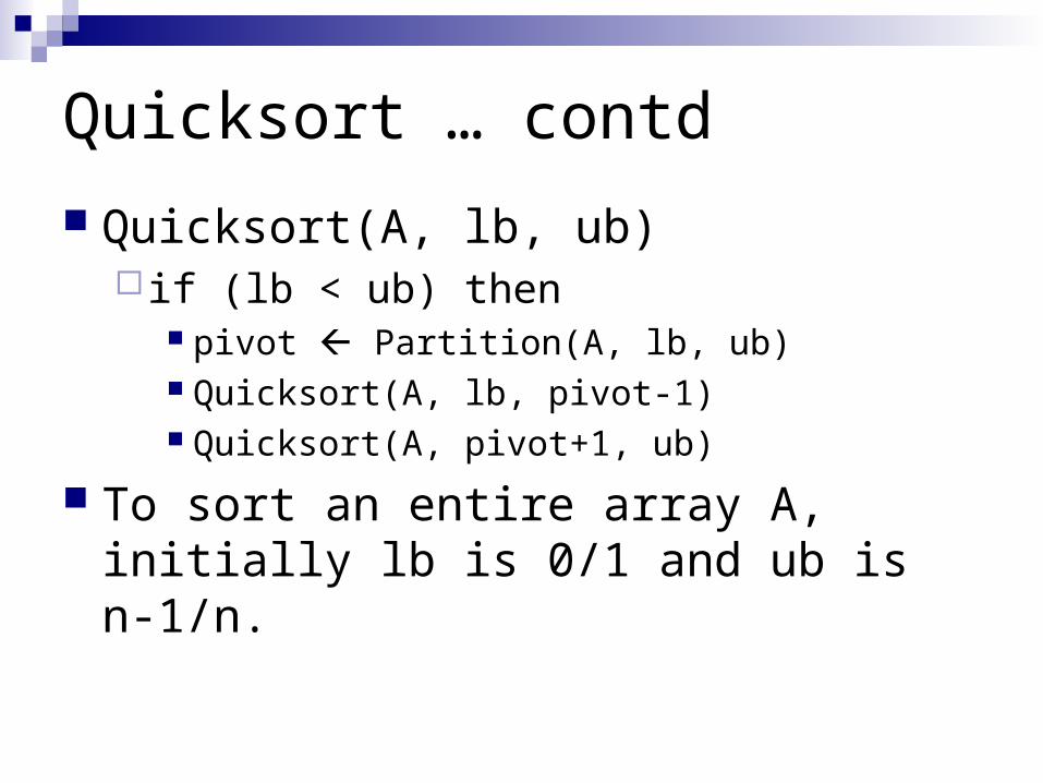
Quicksort … contd Partition(A, lb, ub)

x A[lb] up ub down lb while (down < up) do

while (A[down] ≤ x and down < ub) down down +1

while (A[up] > x) up up – 1

if (down < up) Swap A[down] A[up]

A[lb] A[up] A[up] x Return up

Quicksort … contd40 20 10 80 60 50 7 30 100

40 20 10 80 60 50 7 30 100

down up

40 20 10 80 60 50 7 30 100

updown

40 20 10 80 60 50 7 30 100updown

40 20 10 80 60 50 7 30 100

updown

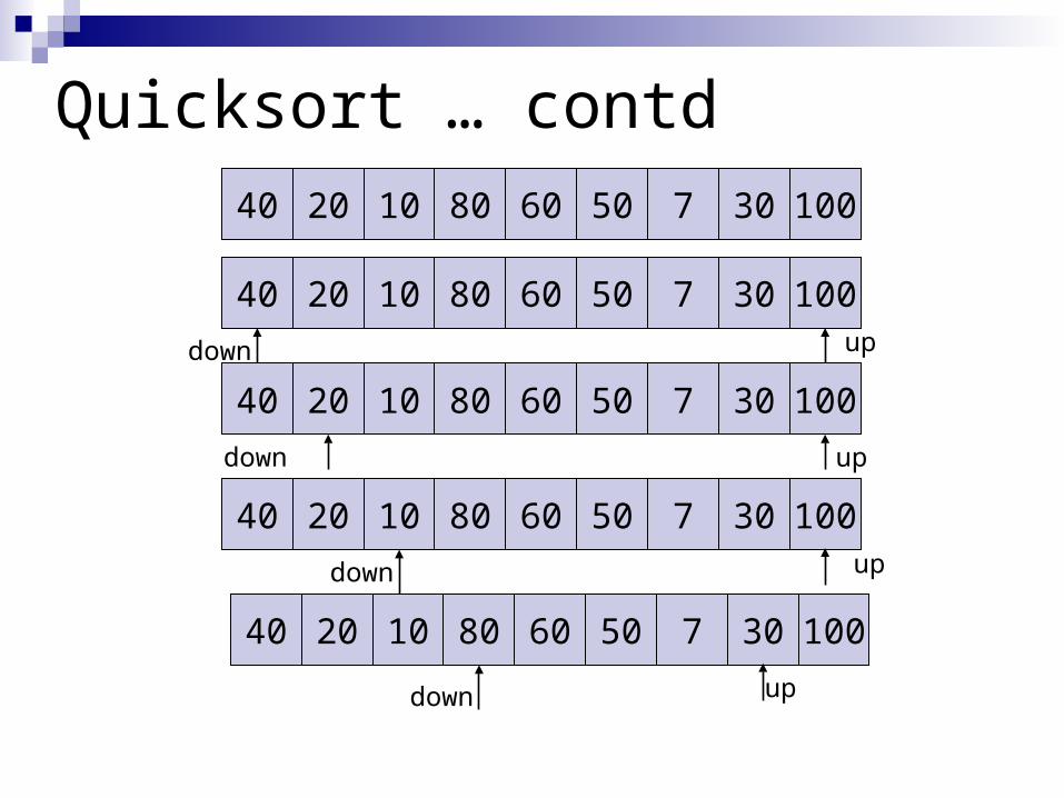
Quicksort …contd

40 20 10 80 60 50 7 30 100

downup

40 20 10 30 60 50 7 80 100

down up

40 20 10 30 60 50 7 80 100

down up

40 20 10 30 60 50 7 80 100

down up

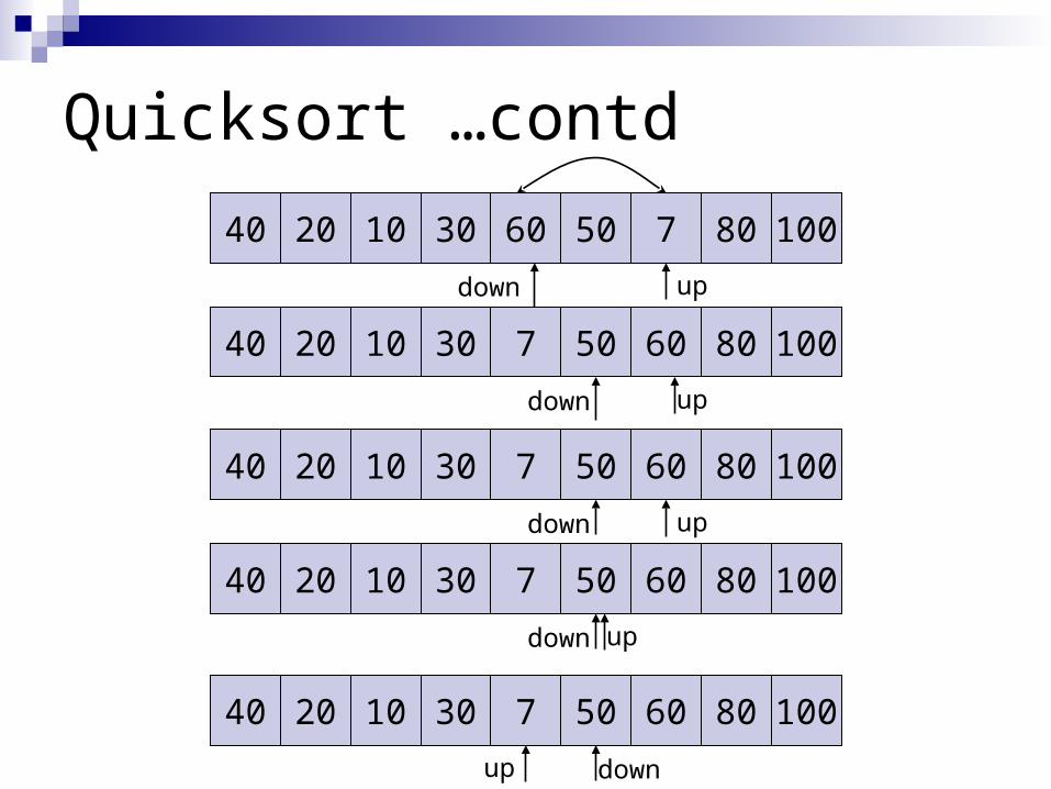
Quicksort …contd

40 20 10 30 60 50 7 80 100

down up

40 20 10 30 7 50 60 80 100

down up

40 20 10 30 7 50 60 80 100

down up

40 20 10 30 7 50 60 80 100

down up

40 20 10 30 7 50 60 80 100

downup

Quicksort … contd

40 20 10 30 7 50 60 80 100

downup

7 20 10 30 7 50 60 80 100

downup

7 20 10 30 40 50 60 80 100

downup

7 20 10 30 40 50 60 80 100

Quicksort … Analysis For analyzing quicksort, we count only

number of element comparisons. Running time

pivot selection: constant time, i.e. O(1)partitioning: linear time, i.e. O(N)running time of the two recursive calls

T(n) = T(i)+T(n-i-1)+cn c is a constant i is the number of elements in the partition.

Quicksort… Analysis

Worst caseComplexity O(n2)

Average CaseComplexity O(nlogn)

ApplicationsCommercial Applications

Randomized Quicksort Choose the pivot randomly (or randomly

permute the input array before sorting). The running time of the algorithm is

independent of input ordering. No specific input elicits worst case

behavior.The worst case depends on the random

number generator. Helps modify Quicksort so that it performs

well on every input.

Randomized Quicksort

R_Quicksort(A, lb, ub) if (lb < ub) then

i Random(lb, ub) Swap A[up] A[i] pivot Partition(A, lb, ub) Quicksort(A, lb, pivot-1) Quicksort(A, pivot+1, ub

Randomized Quicksort … Analysis

Assumptions: all elements are distinct All partitions from 0:n-1 and n-1:0 equally

likely Probability of each partition is 1/n Average case complexity is O(nlogn).

Selection Sort

Successive elements are selected in order and placed in their proper position.

An in-place sort. Simple to implement Works as follows

Find the minimum value in the list Swap it with the value in the first position Repeat the steps abottiove for the remainder of the

list (starting at the second position and advancing each time)

Selection Sort … contd Sel_sort(A, n)

for i 0 to n – 2 k i for j i + 1 to n – 1 //Find the i th smallest element.

if A[j] < A[k] then then k j

if k i then Swap A[i] and A[k]

Selection Sort… Analysis

Selection sort stops when unsorted part becomes empty.

On every step number of unsorted elements decreased by one.

Makes n steps (n is number of elements in array) of outer loop, before stopping.

Number of swaps vary from 0 to n-1 Overall algorithm complexity O(n2).

Radix Sort A sorting algorithm that sorts integers by

processing individual digits, by comparing individual digits sharing the same significant position i.e. radix.

Compares two numbers starting from their LSD till they match

The number with the larger digit in the first position which the digits of the two numbers do not match is the larger of the two.

Radix sort … steps Partition number in ten groups based on

LSD. Can use ten queues for this… say Q[0] –

Q[9]. Merge all the numbers from Q[0] – Q[9] Again perform step 1, now considering the

second LSD Continue till each subgroup has been

subdivided and sorted on MSD.

Radix sort… example

Start with elements of same denomination Read array A of size n E.g.

38, 36, 32, 25, 29, 54, 44, 40 Start by inserting elements in queues

based on LSD

Radix sort… contd

Elements consisting of different number of digits in their values.121, 345, 2, 4343, 12, 34, 5, 1231, 231, 3212

Complexityn elements present take m passes to get

sorted where m is the number of maximum digits in an element.

Order is O(n*m)

Strassen’s Matrix Multiplication The standard method of matrix multiplication of

two n × n matrices takes O(n3) operations. Strassen’s algorithm is a Divide-and-Conquer

algorithm that is asymptotically faster, i.e. O(nlg 7).

The usual multiplication of two 2 × 2 matrices takes 8 multiplications and 4 additions.

Strassen showed how two 2 × 2 matrices can be multiplied using only 7 multiplications and 18 additions.

Basic Matrix Multiplication

Strassen’s Observation

where

Self Study

Finding Min and Max in a list using Divide and Conquer Technique.

Find out other algorithms which can be solved using divide and conquer.

Next

Greedy Method

Documents

DIVIDE AND CONQUER APPROACH. General Method Works on the approach of dividing a given problem into smaller sub problems (ideally of same size). Divide