Embed Size (px)
Citation preview
Diversity in Smartphone Usage
Hossein FalakiCENS, UCLA
Ratul MahajanMicrosoft Research
Srikanth KandulaMicrosoft Research
Dimitrios LymberopoulosMicrosoft Research
Ramesh GovindanCENS, USC
Deborah EstrinCENS, UCLA
Abstract – Using detailed traces from 255 users, we con-duct a comprehensive study of smartphone use. We char-acterize intentional user activities – interactions with thedevice and the applications used – and the impact of thoseactivities on network and energy usage. We find immensediversity among users. Along all aspects that we study, usersdi!er by one or more orders of magnitude. For instance, theaverage number of interactions per day varies from 10 to 200,and the average amount of data received per day varies from1 to 1000 MB. This level of diversity suggests that mecha-nisms to improve user experience or energy consumption willbe more e!ective if they learn and adapt to user behavior.We find that qualitative similarities exist among users thatfacilitate the task of learning user behavior. For instance,the relative application popularity for can be modeled us-ing an exponential distribution, with di!erent distributionparameters for di!erent users. We demonstrate the value ofadapting to user behavior in the context of a mechanism topredict future energy drain. The 90th percentile error withadaptation is less than half compared to predictions basedon average behavior across users.
Categories and Subject DescriptorsC.4 [Performance of systems] Measurement techniques
General TermsMeasurement, human factors
KeywordsSmartphone usage, user behavior
1. INTRODUCTIONSmartphones are being adopted at a phenomenal pace but
little is known (publicly) today about how people use thesedevices. In 2009, smartphone penetration in the US was 25%and 14% of worldwide mobile phone shipments were smart-phones [23, 16]. By 2011, smartphone sales are projected tosurpass desktop PCs [25]. But beyond a few studies that re-port on users’ charging behaviors [2, 17] and relative powerconsumption of various components (e.g., CPU, screen) [24],many basic facts on smartphone usage are unknown: i) howoften does a user interact with the phone and how long does
Permission to make digital or hard copies of all or part of this work forpersonal or classroom use is granted without fee provided that copies arenot made or distributed for profit or commercial advantage and that copiesbear this notice and the full citation on the first page. To copy otherwise, torepublish, to post on servers or to redistribute to lists, requires prior specificpermission and/or a fee.MobiSys’10, June 15–18, 2010, San Francisco, California, USA.Copyright 2010 ACM 978-1-60558-985-5/10/06 ...$10.00.
an interaction last? ii) how many applications does a userrun and how is her attention spread across them? iii) howmuch network tra"c is generated?
Answering such questions is not just a matter of academicinterest; it is key to understanding which mechanisms cane!ectively improve user experience or reduce energy con-sumption. For instance, if user interactions are frequent andthe sleep-wake overhead is significant, putting the phone tosleep aggressively may be counterproductive [8]. If the userinteracts regularly with only a few applications, applicationresponse time can be improved by retaining those applica-tions in memory [7]. Similarly, if most transfers are small,bundling multiple transfers [1, 22] may reduce per-byte en-ergy cost. Smartphone usage will undoubtedly evolve withtime, but understanding current usage is important for in-forming the next generation of devices.
We analyze detailed usage traces from 255 users of twodi!erent smartphone platforms, with 7-28 weeks of data peruser. Our traces consist of two datasets. For the first datasetwe deploy a custom logging utility on the phones of 33 An-droid users. Our utility captures a detailed view of userinteractions, network tra"c, and energy drain. The seconddataset is from 222 Windows Mobile users across di!erentdemographics and geographic locations. This data was col-lected by a third party.
We characterize smartphone usage along four key dimen-sions: i) user interactions; ii) application use; iii) networktra"c; and iv) energy drain. The first two represent inten-tional user activities, and the last two represent the impactof user activities on network and energy resources. Insteadof only exploring average case behaviors, we are interestedin exploring the range seen across users and time. We be-lieve that we are the first to measure and report on manyaspects of smartphone usage of a large population of users.
A recurring theme in our findings is the diversity acrossusers. Along all dimensions that we study, users di!er byone or more orders of magnitude. For example, the meannumber of interactions per day for a user varies from 10 to200; the mean interaction length varies from 10 to 250 sec-onds; the number of applications used varies from 10 to 90;and the mean amount of tra"c per day varies from 1 to1000 MB, of which 10 to 90% is exchanged during inter-active use. We also find that users are along a continuumbetween the extremes, rather than being clustered into asmall number of groups.
The diversity among users that we find stems from thefact that users use their smartphones for di!erent purposesand with di!erent frequencies. For instance, users that use
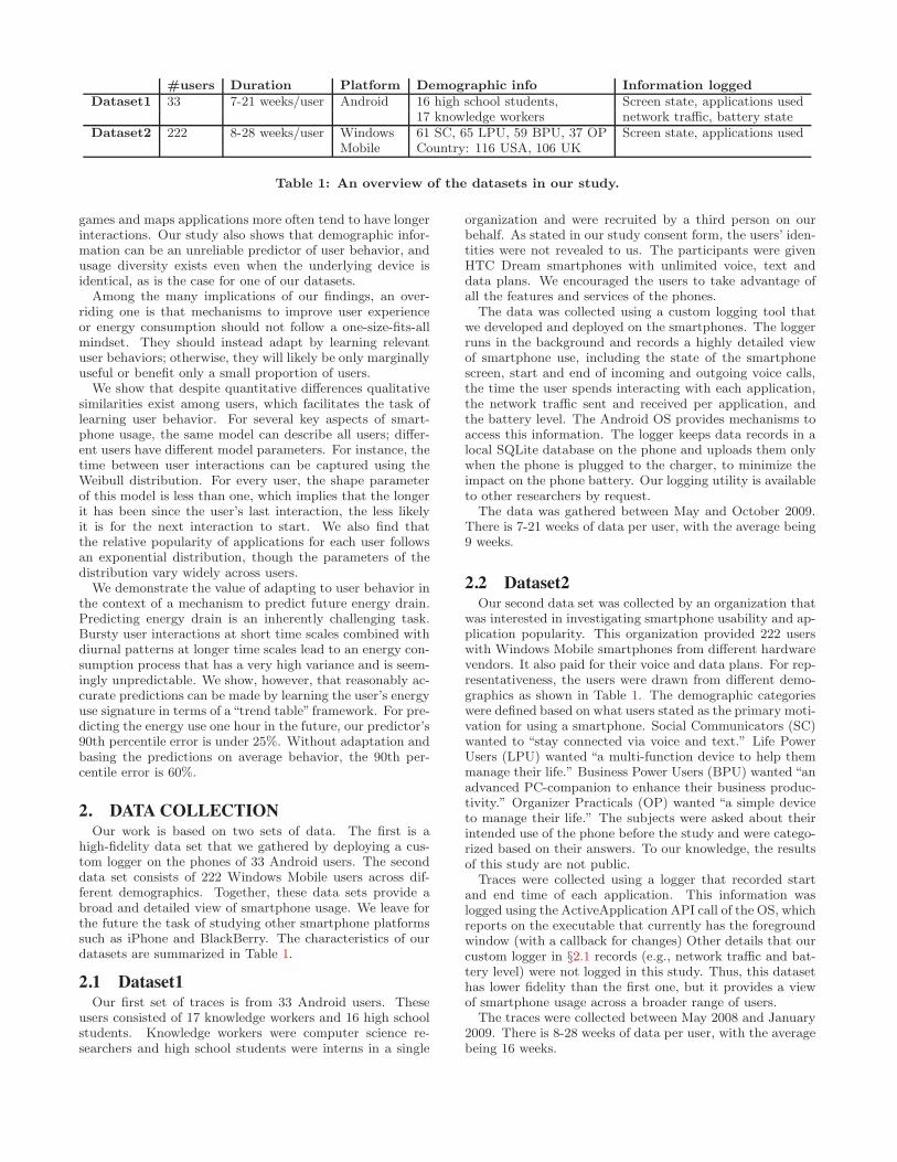
#users Duration Platform Demographic info Information loggedDataset1 33 7-21 weeks/user Android 16 high school students, Screen state, applications used
17 knowledge workers network tra"c, battery stateDataset2 222 8-28 weeks/user Windows 61 SC, 65 LPU, 59 BPU, 37 OP Screen state, applications used
Mobile Country: 116 USA, 106 UK
Table 1: An overview of the datasets in our study.
games and maps applications more often tend to have longerinteractions. Our study also shows that demographic infor-mation can be an unreliable predictor of user behavior, andusage diversity exists even when the underlying device isidentical, as is the case for one of our datasets.
Among the many implications of our findings, an over-riding one is that mechanisms to improve user experienceor energy consumption should not follow a one-size-fits-allmindset. They should instead adapt by learning relevantuser behaviors; otherwise, they will likely be only marginallyuseful or benefit only a small proportion of users.
We show that despite quantitative di!erences qualitativesimilarities exist among users, which facilitates the task oflearning user behavior. For several key aspects of smart-phone usage, the same model can describe all users; di!er-ent users have di!erent model parameters. For instance, thetime between user interactions can be captured using theWeibull distribution. For every user, the shape parameterof this model is less than one, which implies that the longerit has been since the user’s last interaction, the less likelyit is for the next interaction to start. We also find thatthe relative popularity of applications for each user followsan exponential distribution, though the parameters of thedistribution vary widely across users.
We demonstrate the value of adapting to user behavior inthe context of a mechanism to predict future energy drain.Predicting energy drain is an inherently challenging task.Bursty user interactions at short time scales combined withdiurnal patterns at longer time scales lead to an energy con-sumption process that has a very high variance and is seem-ingly unpredictable. We show, however, that reasonably ac-curate predictions can be made by learning the user’s energyuse signature in terms of a“trend table” framework. For pre-dicting the energy use one hour in the future, our predictor’s90th percentile error is under 25%. Without adaptation andbasing the predictions on average behavior, the 90th per-centile error is 60%.
2. DATA COLLECTIONOur work is based on two sets of data. The first is a
high-fidelity data set that we gathered by deploying a cus-tom logger on the phones of 33 Android users. The seconddata set consists of 222 Windows Mobile users across dif-ferent demographics. Together, these data sets provide abroad and detailed view of smartphone usage. We leave forthe future the task of studying other smartphone platformssuch as iPhone and BlackBerry. The characteristics of ourdatasets are summarized in Table 1.
2.1 Dataset1Our first set of traces is from 33 Android users. These
users consisted of 17 knowledge workers and 16 high schoolstudents. Knowledge workers were computer science re-searchers and high school students were interns in a single
organization and were recruited by a third person on ourbehalf. As stated in our study consent form, the users’ iden-tities were not revealed to us. The participants were givenHTC Dream smartphones with unlimited voice, text anddata plans. We encouraged the users to take advantage ofall the features and services of the phones.
The data was collected using a custom logging tool thatwe developed and deployed on the smartphones. The loggerruns in the background and records a highly detailed viewof smartphone use, including the state of the smartphonescreen, start and end of incoming and outgoing voice calls,the time the user spends interacting with each application,the network tra"c sent and received per application, andthe battery level. The Android OS provides mechanisms toaccess this information. The logger keeps data records in alocal SQLite database on the phone and uploads them onlywhen the phone is plugged to the charger, to minimize theimpact on the phone battery. Our logging utility is availableto other researchers by request.
The data was gathered between May and October 2009.There is 7-21 weeks of data per user, with the average being9 weeks.
2.2 Dataset2Our second data set was collected by an organization that
was interested in investigating smartphone usability and ap-plication popularity. This organization provided 222 userswith Windows Mobile smartphones from di!erent hardwarevendors. It also paid for their voice and data plans. For rep-resentativeness, the users were drawn from di!erent demo-graphics as shown in Table 1. The demographic categorieswere defined based on what users stated as the primary moti-vation for using a smartphone. Social Communicators (SC)wanted to “stay connected via voice and text.” Life PowerUsers (LPU) wanted “a multi-function device to help themmanage their life.” Business Power Users (BPU) wanted “anadvanced PC-companion to enhance their business produc-tivity.” Organizer Practicals (OP) wanted “a simple deviceto manage their life.” The subjects were asked about theirintended use of the phone before the study and were catego-rized based on their answers. To our knowledge, the resultsof this study are not public.
Traces were collected using a logger that recorded startand end time of each application. This information waslogged using the ActiveApplication API call of the OS, whichreports on the executable that currently has the foregroundwindow (with a callback for changes) Other details that ourcustom logger in §2.1 records (e.g., network tra"c and bat-tery level) were not logged in this study. Thus, this datasethas lower fidelity than the first one, but it provides a viewof smartphone usage across a broader range of users.
The traces were collected between May 2008 and January2009. There is 8-28 weeks of data per user, with the averagebeing 16 weeks.
0.0
0.2
0.4
0.6
0.8
1.0
0 20 40 60 80 100User percentile
Voic
e us
age
ratio
Dataset1Dataset2
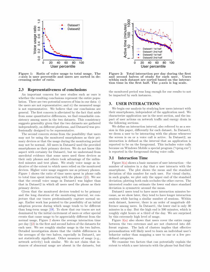
Figure 1: Ratio of voice usage to total usage. Thex-axis is user percentile and users are sorted in de-creasing order of ratio.
2.3 Representativeness of conclusionsAn important concern for user studies such as ours is
whether the resulting conclusions represent the entire popu-lation. There are two potential sources of bias in our data: i)the users are not representative; and ii) the measured usageis not representative. We believe that our conclusions aregeneral. The first concern is alleviated by the fact that asidefrom some quantitative di!erences, we find remarkable con-sistency among users in the two datasets. This consistencysuggests generality given that the two datasets are gatheredindependently, on di!erent platforms, and Dataset2 was pro-fessionally designed to be representative.
The second concern stems from the possibility that usersmay not be using the monitored smartphones as their pri-mary devices or that the usage during the monitoring periodmay not be normal. All users in Dataset2 used the providedsmartphones as their primary devices. We do not know thisaspect with certainty for Dataset1, but we understand fromanecdotal evidence that some users used these devices astheir only phones and others took advantage of the unlim-ited minutes and text plans. We study voice usage as in-dicative of the extent to which users relied on the monitoreddevices. Higher voice usage suggests use as primary phones.Figure 1 shows the ratio of time users spent in phone callsto total time spent interacting with the phone (§3). We seethat the overall voice usage in Dataset1 was higher thanthat in Dataset2 in which all users used the phone as theirprimary device.
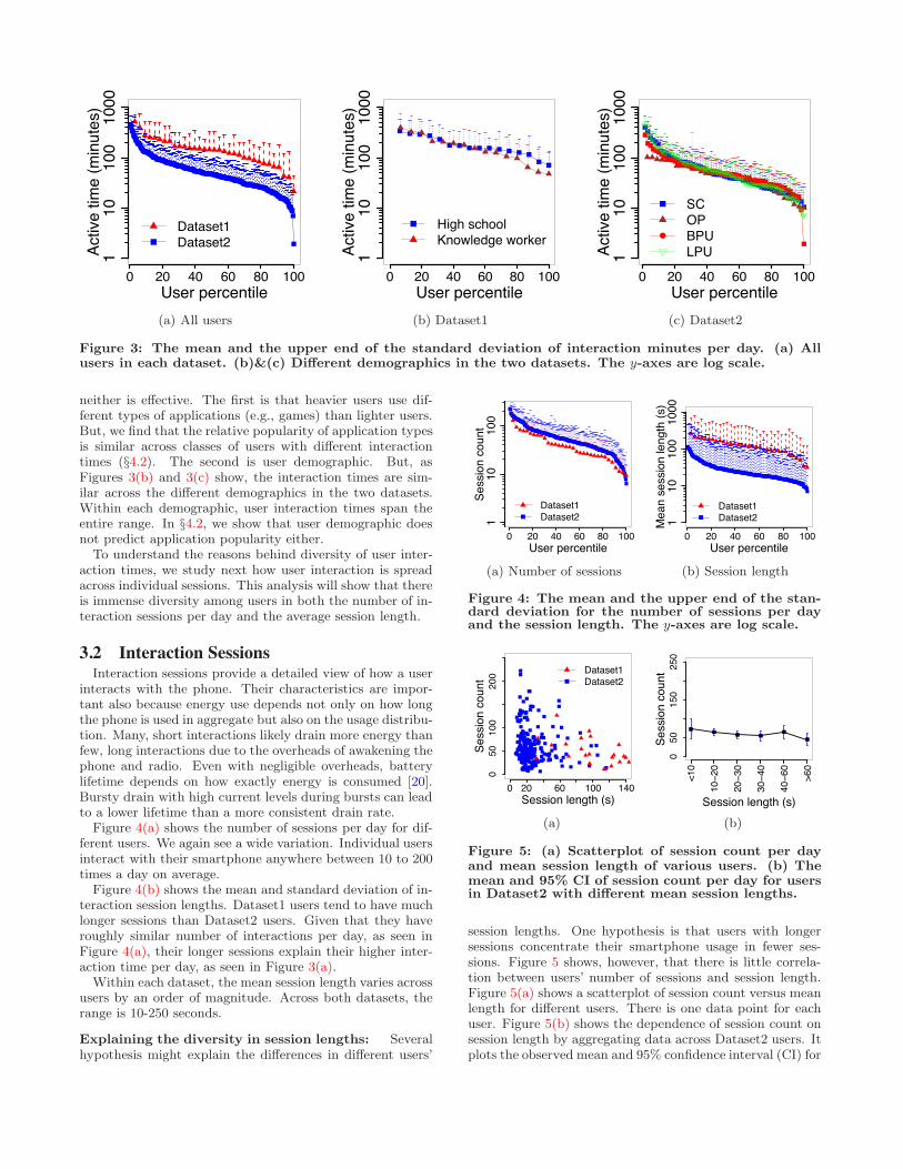
Given that the monitored devices tended to be primaryand the long duration of the monitoring interval, we con-jecture that our traces predominantly capture normal us-age. Earlier work has pointed to the possibility of an initialadoption process during which usage tends to be di!erentthan long-term usage [19]. To show that our traces are notdominated by the initial excitement of users or other specialevents that cause usage to be appreciably di!erent from thenormal usage, Figure 2 shows the average interaction timeper day (§3) in the first and second halves of the datasets foreach user. We see roughly similar usage in the two halves.Detailed investigation shows that the visible di!erences inthe averages of the two halves, especially in Dataset1, arenot statistically significant. Other measures of usage (e.g.,network activity) look similar. We do not claim that in-stances of abnormal usage are absent in the datasets, but
110
100
1000
0 20 40 60 80 100User percentile
Activ
e tim
e (m
inut
es)
Dataset1 1st halfDataset1 2nd halfDataset2 1st halfDataset2 2nd half
Figure 2: Total interaction per day during the firstand second halves of study for each user. Userswithin each dataset are sorted based on the interac-tion time in the first half. The y-axis is log scale.
the monitored period was long enough for our results to notbe impacted by such instances.
3. USER INTERACTIONSWe begin our analysis by studying how users interact with
their smartphones, independent of the application used. Wecharacterize application use in the next section, and the im-pact of user actions on network tra"c and energy drain inthe following sections.
We define an interaction interval, also referred to as a ses-sion in this paper, di!erently for each dataset. In Dataset1,we deem a user to be interacting with the phone wheneverthe screen is on or a voice call is active. In Dataset2, aninteraction is defined as the interval that an application isreported to be on the foreground. This includes voice callsbecause on Windows Mobile a special program (“cprog.exe”)is reported in the foreground during voice calls.
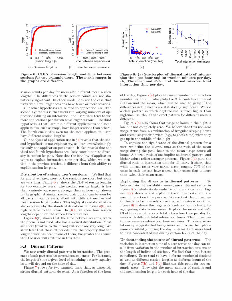
3.1 Interaction TimeFigure 3(a) shows a basic measure of user interaction—the
number of minutes in a day that a user interacts with thesmartphone. The plot shows the mean and the standarddeviation of this number for each user. For visual clarity,in such graphs, we plot only the upper end of the standarddeviation; plotting both ends occludes the other curves. Theinterested reader can estimate the lower end since standarddeviation is symmetric around the mean.
Dataset1 users tend to have more interaction minutes be-cause, as we show later, they tend to have longer interactionsessions while having a similar number of sessions. Withineach dataset, however, there is an order of magnitude dif-ference among users. In Dataset1, the lower end is only 30minutes in a day. But the high end is 500 minutes, which isroughly eight hours or a third of the day. We are surprisedby this extremely high level of usage.
Figure 3(a) also shows that users cover the entire rangebetween the two extremes and are not clustered into dif-ferent regions. The lack of clusters implies that e!ectivepersonalization will likely need to learn an individual user’sbehavior rather than mapping a user to one or a few pre-defined categories.
We examine two factors that can potentially explain theextent to which a user interacts with the phone but find that
110
100
1000
0 20 40 60 80 100User percentile
Activ
e tim
e (m
inut
es)
Dataset1Dataset2
(a) All users
High schoolKnowledge worker
110
100
1000
0 20 40 60 80 100User percentile
Activ
e tim
e (m
inut
es)
(b) Dataset1
SCOPBPULPU1
1010
010
00
0 20 40 60 80 100User percentile
Activ
e tim
e (m
inut
es)
(c) Dataset2
Figure 3: The mean and the upper end of the standard deviation of interaction minutes per day. (a) Allusers in each dataset. (b)&(c) Di!erent demographics in the two datasets. The y-axes are log scale.
neither is e!ective. The first is that heavier users use dif-ferent types of applications (e.g., games) than lighter users.But, we find that the relative popularity of application typesis similar across classes of users with di!erent interactiontimes (§4.2). The second is user demographic. But, asFigures 3(b) and 3(c) show, the interaction times are sim-ilar across the di!erent demographics in the two datasets.Within each demographic, user interaction times span theentire range. In §4.2, we show that user demographic doesnot predict application popularity either.
To understand the reasons behind diversity of user inter-action times, we study next how user interaction is spreadacross individual sessions. This analysis will show that thereis immense diversity among users in both the number of in-teraction sessions per day and the average session length.
3.2 Interaction SessionsInteraction sessions provide a detailed view of how a user
interacts with the phone. Their characteristics are impor-tant also because energy use depends not only on how longthe phone is used in aggregate but also on the usage distribu-tion. Many, short interactions likely drain more energy thanfew, long interactions due to the overheads of awakening thephone and radio. Even with negligible overheads, batterylifetime depends on how exactly energy is consumed [20].Bursty drain with high current levels during bursts can leadto a lower lifetime than a more consistent drain rate.
Figure 4(a) shows the number of sessions per day for dif-ferent users. We again see a wide variation. Individual usersinteract with their smartphone anywhere between 10 to 200times a day on average.
Figure 4(b) shows the mean and standard deviation of in-teraction session lengths. Dataset1 users tend to have muchlonger sessions than Dataset2 users. Given that they haveroughly similar number of interactions per day, as seen inFigure 4(a), their longer sessions explain their higher inter-action time per day, as seen in Figure 3(a).
Within each dataset, the mean session length varies acrossusers by an order of magnitude. Across both datasets, therange is 10-250 seconds.
Explaining the diversity in session lengths: Severalhypothesis might explain the di!erences in di!erent users’
Dataset1Dataset21
1010
0
0 20 40 60 80 100User percentile
Sess
ion
coun
t
(a) Number of sessions
110
100
1000
0 20 40 60 80 100User percentile
Mea
n se
ssio
n le
ngth
(s)
Dataset1Dataset2
(b) Session length
Figure 4: The mean and the upper end of the stan-dard deviation for the number of sessions per dayand the session length. The y-axes are log scale.
050
100
200
0 20 60 100 140Session length (s)
Sess
ion
coun
t
Dataset1Dataset2
(a)
050
150
250
Sess
ion
coun
t
<10
10−2
0
20−3
0
30−4
0
40−6
0
>60
Session length (s)
(b)
Figure 5: (a) Scatterplot of session count per dayand mean session length of various users. (b) Themean and 95% CI of session count per day for usersin Dataset2 with di!erent mean session lengths.
session lengths. One hypothesis is that users with longersessions concentrate their smartphone usage in fewer ses-sions. Figure 5 shows, however, that there is little correla-tion between users’ number of sessions and session length.Figure 5(a) shows a scatterplot of session count versus meanlength for di!erent users. There is one data point for eachuser. Figure 5(b) shows the dependence of session count onsession length by aggregating data across Dataset2 users. Itplots the observed mean and 95% confidence interval (CI) for
Dataset1 example userDataset2 example user
0.0
0.2
0.4
0.6
0.8
1.0
0 200 600 1000Session length (s)
CD
F
(a) Session lengths
Dataset1 example userDataset2 example user
0.0
0.2
0.4
0.6
0.8
1.0
0 1000 2000 3000Time between sessions (s)
CD
F(b) Time between sessions
Figure 6: CDFs of session length and time betweensessions for two example users. The x-axis ranges inthe graphs are di!erent.
session counts per day for users with di!erent mean sessionlengths. The di!erences in the session counts are not sta-tistically significant. In other words, it is not the case thatusers who have longer sessions have fewer or more sessions.
Our other hypotheses are related to application use. Thesecond hypothesis is that users run varying numbers of ap-plications during an interaction, and users that tend to usemore applications per session have longer sessions. The thirdhypothesis is that users run di!erent applications and someapplications, such as maps, have longer sessions than others.The fourth one is that even for the same application, usershave di!erent session lengths.
Our analysis of application use in §4 reveals that the sec-ond hypothesis is not explanatory, as users overwhelminglyuse only one application per session. It also reveals that thethird and fourth hypotheses are likely contributors to diver-sity in session lengths. Note that the inability of applicationtypes to explain interaction time per day, which we men-tion in the previous section, is di!erent from their ability toexplain session lengths.
Distribution of a single user’s sessions: We find thatfor any given user, most of the sessions are short but someare very long. Figure 6(a) shows the CDF of session lengthsfor two example users. The median session length is lessthan a minute but some are longer than an hour (not shownin the graph). A similar skewed distribution can be seen forall users in our datasets, albeit with di!erent median andmean session length values. This highly skewed distributionalso explains why the standard deviations in Figure 4(b) arehigh relative to the mean. In §8.1, we show how sessionlengths depend on the screen timeout values.
Figure 6(b) shows that the time between sessions, whenthe phone is not used, also has a skewed distribution. Mostare short (relative to the mean) but some are very long. Weshow later that these o! periods have the property that thelonger a user has been in one of them, the greater the chancethat the user will continue in this state.
3.3 Diurnal PatternsWe now study diurnal patterns in interaction. The pres-
ence of such patterns has several consequences. For instance,the length of time a given level of remaining battery capacitylasts will depend on the time of day.
Figure 7 shows for two example users that, as expected,strong diurnal patterns do exist. As a function of the hour
Dataset1Dataset2
16
1116
21
0 100 200 300 400Total interaction (minutes)
Diu
rnal
ratio
(a)
<30
30−6
060−9
090−1
2012
0−15
015
0−20
020
0−30
0>3
00
01
23
45
Diu
rnal
ratio
Total interaction (minutes)
(b)
Figure 8: (a) Scatterplot of diurnal ratio of interac-tion time per hour and interaction minutes per day.(b) The mean and 95% CI of diurnal ratio vs. totalinteraction time per day.
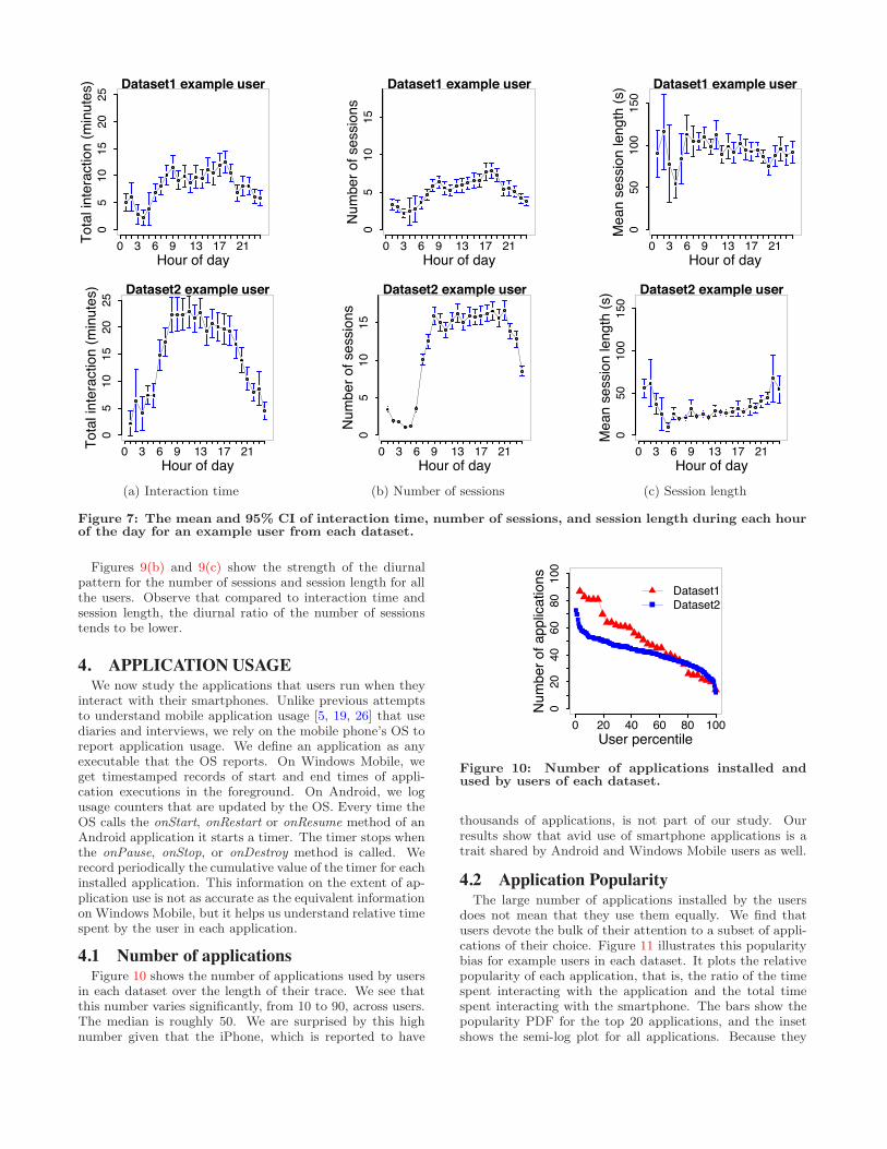
of the day, Figure 7(a) plots the mean number of interactionminutes per hour. It also plots the 95% confidence interval(CI) around the mean, which can be used to judge if thedi!erences in the means are statistically significant. We seea clear pattern in which daytime use is much higher thannightime use, though the exact pattern for di!erent users isdi!erent.
Figure 7(a) also shows that usage at hours in the night islow but not completely zero. We believe that this non-zerousage stems from a combination of irregular sleeping hoursand users using their devices (e.g., to check time) when theyget up in the middle of the night.
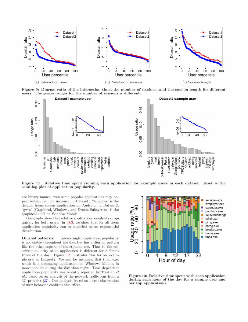
To capture the significance of the diurnal pattern for auser, we define the diurnal ratio as the ratio of the meanusage during the peak hour to the mean usage across allhours. A diurnal ratio of one implies no diurnal pattern, andhigher values reflect stronger patterns. Figure 9(a) plots thediurnal ratio in interaction time for all users. It shows thatwhile diurnal ratios vary across users, roughly 70% of theusers in each dataset have a peak hour usage that is morethan twice their mean usage.
Explaining the diversity in diurnal patterns: Tohelp explain the variability among users’ diurnal ratios, inFigure 8 we study its dependence on interaction time. Fig-ure 8(a) shows a scatterplot of the diurnal ratio and themean interaction time per day. We see that the diurnal ra-tio tends to be inversely correlated with interaction time.Figure 8(b) shows this negative correlation more clearly, byaggregating data across users. It plots the mean and 95%CI of the diurnal ratio of total interaction time per day forusers with di!erent total interaction times. The diurnal ra-tio decreases as interaction time increases. This inverse re-lationship suggests that heavy users tend to use their phonemore consistently during the day whereas light users tendto have concentrated use during certain hours of the day.
Understanding the source of diurnal patterns: Thevariation in interaction time of a user across the day can re-sult from variation in the number of interaction sessions orthe length of individual sessions. We find that both factorscontribute. Users tend to have di!erent number of sessionsas well as di!erent session lengths at di!erent hours of theday. Figures 7(b) and 7(c) illustrate this point for two ex-ample users. They plot the mean number of sessions andthe mean session length for each hour of the day.
Dataset1 example user0
510
1520
25
0 3 6 9 13 17 21Hour of day
Tota
l int
erac
tion
(min
utes
) Dataset1 example user
05
1015
0 3 6 9 13 17 21Hour of day
Num
ber o
f ses
sion
s
Dataset1 example user
050
100
150
0 3 6 9 13 17 21Hour of day
Mea
n se
ssio
n le
ngth
(s)
Dataset2 example user
05
1015
2025
0 3 6 9 13 17 21Hour of day
Tota
l int
erac
tion
(min
utes
)
(a) Interaction time
Dataset2 example user
05
1015
0 3 6 9 13 17 21Hour of day
Num
ber o
f ses
sion
s
(b) Number of sessions
Dataset2 example user
050
100
150
0 3 6 9 13 17 21Hour of day
Mea
n se
ssio
n le
ngth
(s)
(c) Session length
Figure 7: The mean and 95% CI of interaction time, number of sessions, and session length during each hourof the day for an example user from each dataset.
Figures 9(b) and 9(c) show the strength of the diurnalpattern for the number of sessions and session length for allthe users. Observe that compared to interaction time andsession length, the diurnal ratio of the number of sessionstends to be lower.
4. APPLICATION USAGEWe now study the applications that users run when they
interact with their smartphones. Unlike previous attemptsto understand mobile application usage [5, 19, 26] that usediaries and interviews, we rely on the mobile phone’s OS toreport application usage. We define an application as anyexecutable that the OS reports. On Windows Mobile, weget timestamped records of start and end times of appli-cation executions in the foreground. On Android, we logusage counters that are updated by the OS. Every time theOS calls the onStart, onRestart or onResume method of anAndroid application it starts a timer. The timer stops whenthe onPause, onStop, or onDestroy method is called. Werecord periodically the cumulative value of the timer for eachinstalled application. This information on the extent of ap-plication use is not as accurate as the equivalent informationon Windows Mobile, but it helps us understand relative timespent by the user in each application.
4.1 Number of applicationsFigure 10 shows the number of applications used by users
in each dataset over the length of their trace. We see thatthis number varies significantly, from 10 to 90, across users.The median is roughly 50. We are surprised by this highnumber given that the iPhone, which is reported to have
020
4060
8010
0
0 20 40 60 80 100User percentile
Num
ber o
f app
licat
ions
Dataset1Dataset2
Figure 10: Number of applications installed andused by users of each dataset.
thousands of applications, is not part of our study. Ourresults show that avid use of smartphone applications is atrait shared by Android and Windows Mobile users as well.
4.2 Application PopularityThe large number of applications installed by the users
does not mean that they use them equally. We find thatusers devote the bulk of their attention to a subset of appli-cations of their choice. Figure 11 illustrates this popularitybias for example users in each dataset. It plots the relativepopularity of each application, that is, the ratio of the timespent interacting with the application and the total timespent interacting with the smartphone. The bars show thepopularity PDF for the top 20 applications, and the insetshows the semi-log plot for all applications. Because they
15
913
1721
0 20 40 60 80 100User percentile
Diu
rnal
ratio
Dataset1Dataset2
(a) Interaction time
12
34
5
0 20 40 60 80 100User percentile
Diu
rnal
ratio
Dataset1Dataset2
(b) Number of sessions
15
913
1721
0 20 40 60 80 100User percentile
Diu
rnal
ratio
Dataset1Dataset2
(c) Session length
Figure 9: Diurnal ratio of the interaction time, the number of sessions, and the session length for di!erentusers. The y-axis ranges for the number of sessions is di!erent.
laun
cher gm
alar
mcl
ock
talk
cont
acts
map
sm
ms
phon
em
usic
brow
ser
cam
era
syst
emse
nsbe
nchm
ark
wer
tago
vend
ing
cale
ndar
setti
ngs
tippi
ntim
ete
tris
andr
oid
Dataset1 example user
Usa
ge ra
tio0.
000.
100.
200.
30
0 20 401e−0
70.
01
iexp
lore
gwes
tmai
lho
me
bubb
lebr
eake
rPo
ker
Live
Sear
chca
lend
arG
oogl
eMap
spo
utlo
okTP
CSo
litar
eKa
Glo
mpv
bloa
dcp
rog
serv
ices
tels
hell
pim
gap
pman
YGoN
etw
mpl
ayer
Dataset2 example user
Usa
ge ra
tio0.
000.
050.
100.
150 20 40 601e
−06
0.01
Figure 11: Relative time spent running each application for example users in each dataset. Inset is thesemi-log plot of application popularity.
are binary names, even some popular applications may ap-pear unfamiliar. For instance, in Dataset1, “launcher” is thedefault home screen application on Android; in Dataset2,“gwes” (Graphical, Windows, and Events Subsystem) is thegraphical shell on Window Mobile.
The graphs show that relative application popularity dropsquickly for both users. In §8.3, we show that for all usersapplication popularity can be modeled by an exponentialdistribution.
Diurnal patterns: Interestingly, application popularityis not stable throughout the day, but has a diurnal patternlike the other aspects of smartphone use. That is, the rel-ative popularity of an application is di!erent for di!erenttimes of the day. Figure 12 illustrates this for an exam-ple user in Dataset2. We see, for instance, that tmail.exe,which is a messaging application on Windows Mobile, ismore popular during the day than night. Time dependentapplication popularity was recently reported by Trestian etal., based on an analysis of the network tra"c logs from a3G provider [27]. Our analysis based on direct observationof user behavior confirms this e!ect.
0 4 8 12 17 22Hour of day
020
4060
80U
sage
ratio
(%)
services.exewmplayer.execalendar.exepoutlook.exeWLMMessengercdial.exepimg.execprog.exeiexplore.exehome.exetmail.exe
Figure 12: Relative time spent with each applicationduring each hour of the day for a sample user andher top applications.
comm. 44%
browsing 10%
other 11%
prod. 19%media 5%
maps 5%games 2%system 5%
Dataset1
comm. 49%
browsing 12% other 15%prod. 2%
media 9%maps 2%
games 10%system 1%
Dataset2
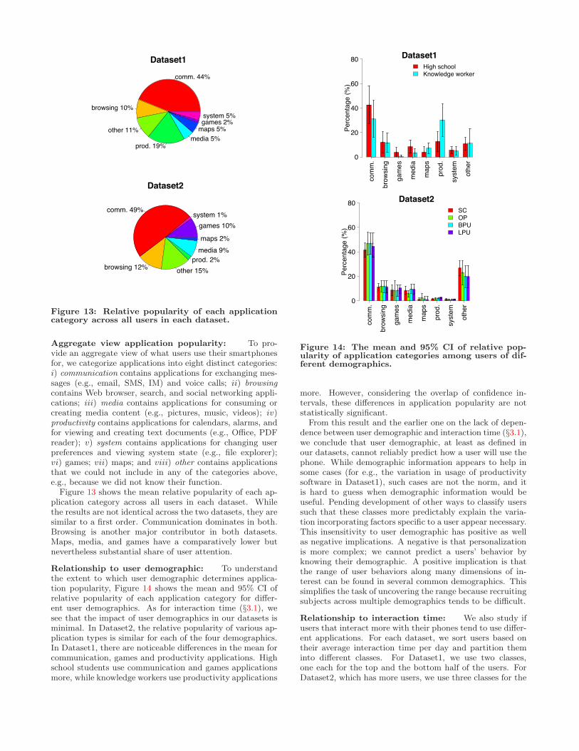
Figure 13: Relative popularity of each applicationcategory across all users in each dataset.
Aggregate view application popularity: To pro-vide an aggregate view of what users use their smartphonesfor, we categorize applications into eight distinct categories:i) communication contains applications for exchanging mes-sages (e.g., email, SMS, IM) and voice calls; ii) browsingcontains Web browser, search, and social networking appli-cations; iii) media contains applications for consuming orcreating media content (e.g., pictures, music, videos); iv)productivity contains applications for calendars, alarms, andfor viewing and creating text documents (e.g., O"ce, PDFreader); v) system contains applications for changing userpreferences and viewing system state (e.g., file explorer);vi) games; vii) maps; and viii) other contains applicationsthat we could not include in any of the categories above,e.g., because we did not know their function.
Figure 13 shows the mean relative popularity of each ap-plication category across all users in each dataset. Whilethe results are not identical across the two datasets, they aresimilar to a first order. Communication dominates in both.Browsing is another major contributor in both datasets.Maps, media, and games have a comparatively lower butnevertheless substantial share of user attention.
Relationship to user demographic: To understandthe extent to which user demographic determines applica-tion popularity, Figure 14 shows the mean and 95% CI ofrelative popularity of each application category for di!er-ent user demographics. As for interaction time (§3.1), wesee that the impact of user demographics in our datasets isminimal. In Dataset2, the relative popularity of various ap-plication types is similar for each of the four demographics.In Dataset1, there are noticeable di!erences in the mean forcommunication, games and productivity applications. Highschool students use communication and games applicationsmore, while knowledge workers use productivity applications
Dataset1
Perc
enta
ge (%
)
0
20
40
60
80
com
m.
brow
sing
gam
es
med
ia
map
s
prod
.
syst
em
othe
r
High schoolKnowledge worker
Dataset2
Perc
enta
ge (%
)
0
20
40
60
80
com
m.
brow
sing
gam
es
med
ia
map
s
prod
.
syst
em
othe
r
SCOPBPULPU
Figure 14: The mean and 95% CI of relative pop-ularity of application categories among users of dif-ferent demographics.
more. However, considering the overlap of confidence in-tervals, these di!erences in application popularity are notstatistically significant.
From this result and the earlier one on the lack of depen-dence between user demographic and interaction time (§3.1),we conclude that user demographic, at least as defined inour datasets, cannot reliably predict how a user will use thephone. While demographic information appears to help insome cases (for e.g., the variation in usage of productivitysoftware in Dataset1), such cases are not the norm, and itis hard to guess when demographic information would beuseful. Pending development of other ways to classify userssuch that these classes more predictably explain the varia-tion incorporating factors specific to a user appear necessary.This insensitivity to user demographic has positive as wellas negative implications. A negative is that personalizationis more complex; we cannot predict a users’ behavior byknowing their demographic. A positive implication is thatthe range of user behaviors along many dimensions of in-terest can be found in several common demographics. Thissimplifies the task of uncovering the range because recruitingsubjects across multiple demographics tends to be di"cult.
Relationship to interaction time: We also study ifusers that interact more with their phones tend to use di!er-ent applications. For each dataset, we sort users based ontheir average interaction time per day and partition theminto di!erent classes. For Dataset1, we use two classes,one each for the top and the bottom half of the users. ForDataset2, which has more users, we use three classes for the
Dataset1
Perc
enta
ge (%
)
0
20
40
60
80
com
m.
brow
sing
gam
es
med
ia
map
s
prod
.
syst
em
othe
r
HighLow
Dataset2
Perc
enta
ge (%
)
0
20
40
60
80
com
m.
brow
sing
gam
es
med
ia
map
s
prod
.
syst
em
othe
rHighMediumLow
Figure 15: The mean and 95% CI of relative pop-ularity of application categories among di!erentclasses of users based on interaction time per day.
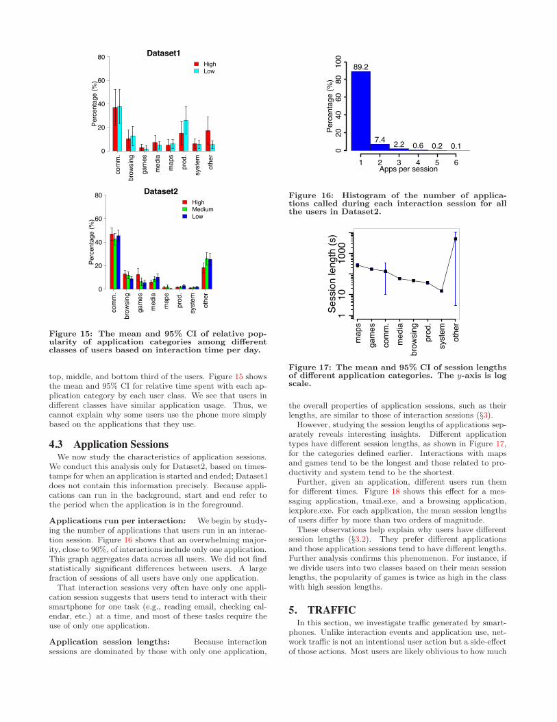
top, middle, and bottom third of the users. Figure 15 showsthe mean and 95% CI for relative time spent with each ap-plication category by each user class. We see that users indi!erent classes have similar application usage. Thus, wecannot explain why some users use the phone more simplybased on the applications that they use.
4.3 Application SessionsWe now study the characteristics of application sessions.
We conduct this analysis only for Dataset2, based on times-tamps for when an application is started and ended; Dataset1does not contain this information precisely. Because appli-cations can run in the background, start and end refer tothe period when the application is in the foreground.
Applications run per interaction: We begin by study-ing the number of applications that users run in an interac-tion session. Figure 16 shows that an overwhelming major-ity, close to 90%, of interactions include only one application.This graph aggregates data across all users. We did not findstatistically significant di!erences between users. A largefraction of sessions of all users have only one application.
That interaction sessions very often have only one appli-cation session suggests that users tend to interact with theirsmartphone for one task (e.g., reading email, checking cal-endar, etc.) at a time, and most of these tasks require theuse of only one application.
Application session lengths: Because interactionsessions are dominated by those with only one application,
89.2
7.4 2.2 0.6 0.2 0.1
1 2 3 4 5 6
020
4060
8010
0
Apps per session
Perc
enta
ge (%
)
Figure 16: Histogram of the number of applica-tions called during each interaction session for allthe users in Dataset2.
map
sga
mes
com
m.
med
iabr
owsi
ngpr
od.
syst
emot
her
110
1000
Sess
ion
leng
th (s
)
Figure 17: The mean and 95% CI of session lengthsof di!erent application categories. The y-axis is logscale.
the overall properties of application sessions, such as theirlengths, are similar to those of interaction sessions (§3).
However, studying the session lengths of applications sep-arately reveals interesting insights. Di!erent applicationtypes have di!erent session lengths, as shown in Figure 17,for the categories defined earlier. Interactions with mapsand games tend to be the longest and those related to pro-ductivity and system tend to be the shortest.
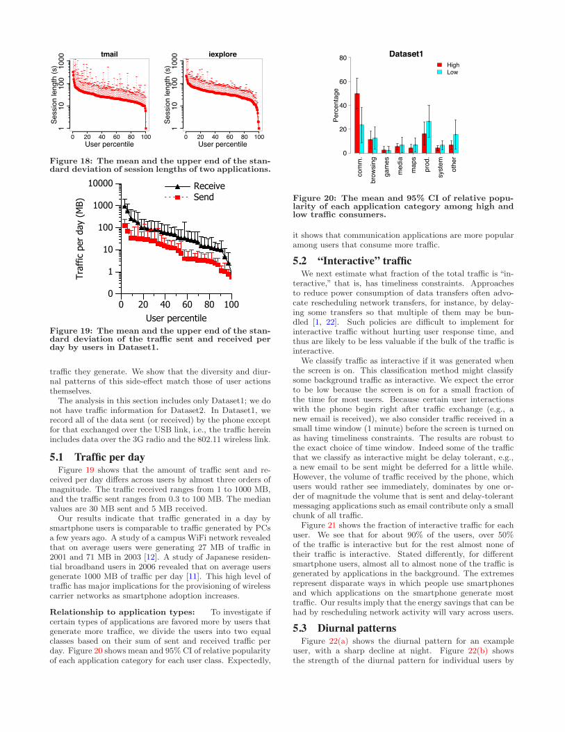
Further, given an application, di!erent users run themfor di!erent times. Figure 18 shows this e!ect for a mes-saging application, tmail.exe, and a browsing application,iexplore.exe. For each application, the mean session lengthsof users di!er by more than two orders of magnitude.
These observations help explain why users have di!erentsession lengths (§3.2). They prefer di!erent applicationsand those application sessions tend to have di!erent lengths.Further analysis confirms this phenomenon. For instance, ifwe divide users into two classes based on their mean sessionlengths, the popularity of games is twice as high in the classwith high session lengths.
5. TRAFFICIn this section, we investigate tra"c generated by smart-
phones. Unlike interaction events and application use, net-work tra"c is not an intentional user action but a side-e!ectof those actions. Most users are likely oblivious to how much
tmail1
1010
010
00
0 20 40 60 80 100User percentile
Sess
ion
leng
th (s
)iexplore
110
100
1000
0 20 40 60 80 100User percentile
Sess
ion
leng
th (s
)Figure 18: The mean and the upper end of the stan-dard deviation of session lengths of two applications.
0 20 40 60 80 100User percentile
0
1
10
100
1000
10000
Traf
fic p
er d
ay (
MB)
ReceiveSend
Figure 19: The mean and the upper end of the stan-dard deviation of the tra"c sent and received perday by users in Dataset1.
tra"c they generate. We show that the diversity and diur-nal patterns of this side-e!ect match those of user actionsthemselves.
The analysis in this section includes only Dataset1; we donot have tra"c information for Dataset2. In Dataset1, werecord all of the data sent (or received) by the phone exceptfor that exchanged over the USB link, i.e., the tra"c hereinincludes data over the 3G radio and the 802.11 wireless link.
5.1 Traffic per dayFigure 19 shows that the amount of tra"c sent and re-
ceived per day di!ers across users by almost three orders ofmagnitude. The tra"c received ranges from 1 to 1000 MB,and the tra"c sent ranges from 0.3 to 100 MB. The medianvalues are 30 MB sent and 5 MB received.
Our results indicate that tra"c generated in a day bysmartphone users is comparable to tra"c generated by PCsa few years ago. A study of a campus WiFi network revealedthat on average users were generating 27 MB of tra"c in2001 and 71 MB in 2003 [12]. A study of Japanese residen-tial broadband users in 2006 revealed that on average usersgenerate 1000 MB of tra"c per day [11]. This high level oftra"c has major implications for the provisioning of wirelesscarrier networks as smartphone adoption increases.
Relationship to application types: To investigate ifcertain types of applications are favored more by users thatgenerate more tra"ce, we divide the users into two equalclasses based on their sum of sent and received tra"c perday. Figure 20 shows mean and 95% CI of relative popularityof each application category for each user class. Expectedly,
Dataset1
Perc
enta
ge
0
20
40
60
80
com
m.
brow
sing
gam
es
med
ia
map
s
prod
.
syst
em
othe
r
HighLow
Figure 20: The mean and 95% CI of relative popu-larity of each application category among high andlow tra"c consumers.
it shows that communication applications are more popularamong users that consume more tra"c.
5.2 “Interactive” trafficWe next estimate what fraction of the total tra"c is “in-
teractive,” that is, has timeliness constraints. Approachesto reduce power consumption of data transfers often advo-cate rescheduling network transfers, for instance, by delay-ing some transfers so that multiple of them may be bun-dled [1, 22]. Such policies are di"cult to implement forinteractive tra"c without hurting user response time, andthus are likely to be less valuable if the bulk of the tra"c isinteractive.
We classify tra"c as interactive if it was generated whenthe screen is on. This classification method might classifysome background tra"c as interactive. We expect the errorto be low because the screen is on for a small fraction ofthe time for most users. Because certain user interactionswith the phone begin right after tra"c exchange (e.g., anew email is received), we also consider tra"c received in asmall time window (1 minute) before the screen is turned onas having timeliness constraints. The results are robust tothe exact choice of time window. Indeed some of the tra"cthat we classify as interactive might be delay tolerant, e.g.,a new email to be sent might be deferred for a little while.However, the volume of tra"c received by the phone, whichusers would rather see immediately, dominates by one or-der of magnitude the volume that is sent and delay-tolerantmessaging applications such as email contribute only a smallchunk of all tra"c.
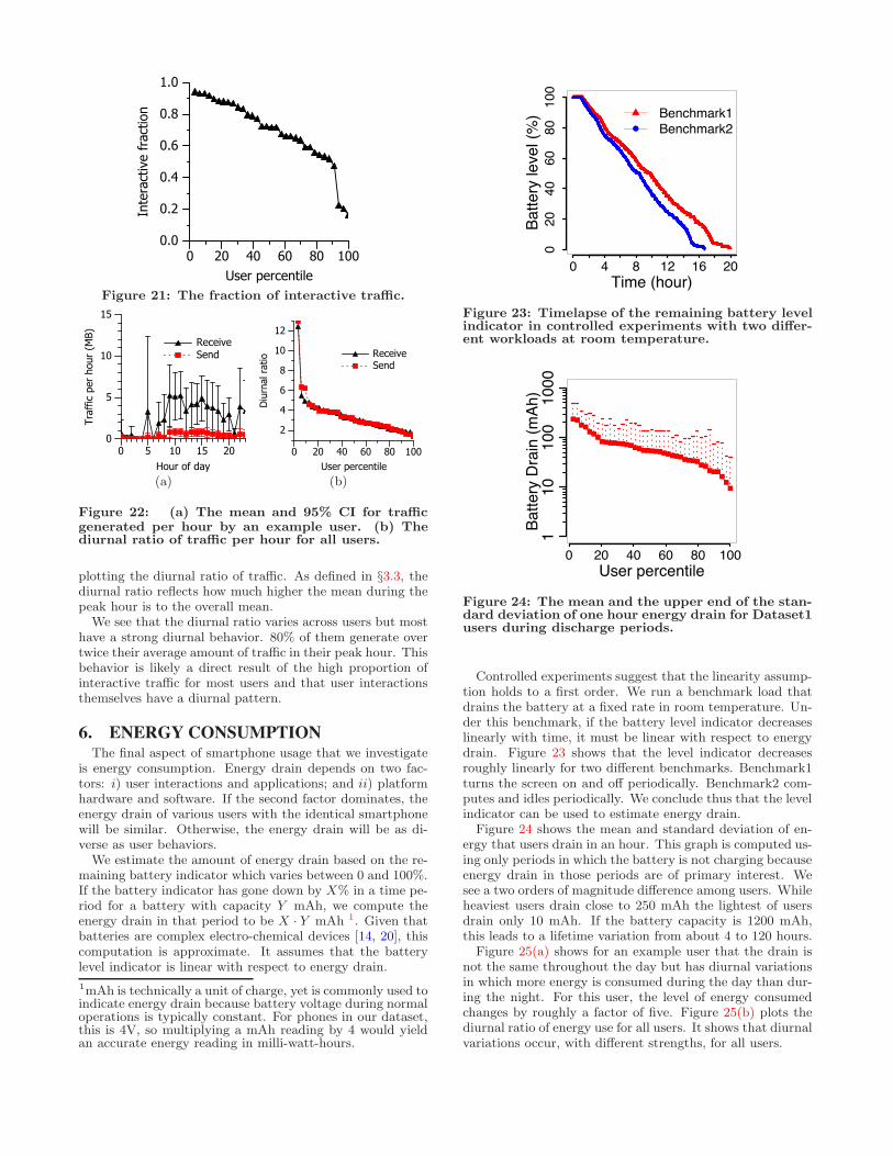
Figure 21 shows the fraction of interactive tra"c for eachuser. We see that for about 90% of the users, over 50%of the tra"c is interactive but for the rest almost none oftheir tra"c is interactive. Stated di!erently, for di!erentsmartphone users, almost all to almost none of the tra"c isgenerated by applications in the background. The extremesrepresent disparate ways in which people use smartphonesand which applications on the smartphone generate mosttra"c. Our results imply that the energy savings that can behad by rescheduling network activity will vary across users.
5.3 Diurnal patternsFigure 22(a) shows the diurnal pattern for an example
user, with a sharp decline at night. Figure 22(b) showsthe strength of the diurnal pattern for individual users by
0 20 40 60 80 100User percentile
0.0
0.2
0.4
0.6
0.8
1.0
Inte
ract
ive
frac
tion
Figure 21: The fraction of interactive tra"c.
0 5 10 15 20Hour of day
0
5
10
15
Traf
fic p
er h
our
(MB)
ReceiveSend
(a)
0 20 40 60 80 100User percentile
2
4
6
8
10
12
Diu
rnal
rat
io ReceiveSend
(b)
Figure 22: (a) The mean and 95% CI for tra"cgenerated per hour by an example user. (b) Thediurnal ratio of tra"c per hour for all users.
plotting the diurnal ratio of tra"c. As defined in §3.3, thediurnal ratio reflects how much higher the mean during thepeak hour is to the overall mean.
We see that the diurnal ratio varies across users but mosthave a strong diurnal behavior. 80% of them generate overtwice their average amount of tra"c in their peak hour. Thisbehavior is likely a direct result of the high proportion ofinteractive tra"c for most users and that user interactionsthemselves have a diurnal pattern.
6. ENERGY CONSUMPTIONThe final aspect of smartphone usage that we investigate
is energy consumption. Energy drain depends on two fac-tors: i) user interactions and applications; and ii) platformhardware and software. If the second factor dominates, theenergy drain of various users with the identical smartphonewill be similar. Otherwise, the energy drain will be as di-verse as user behaviors.
We estimate the amount of energy drain based on the re-maining battery indicator which varies between 0 and 100%.If the battery indicator has gone down by X% in a time pe-riod for a battery with capacity Y mAh, we compute theenergy drain in that period to be X · Y mAh 1. Given thatbatteries are complex electro-chemical devices [14, 20], thiscomputation is approximate. It assumes that the batterylevel indicator is linear with respect to energy drain.
1mAh is technically a unit of charge, yet is commonly used toindicate energy drain because battery voltage during normaloperations is typically constant. For phones in our dataset,this is 4V, so multiplying a mAh reading by 4 would yieldan accurate energy reading in milli-watt-hours.
020
4060
8010
0
0 4 8 12 16 20Time (hour)
Batte
ry le
vel (
%) Benchmark1
Benchmark2
Figure 23: Timelapse of the remaining battery levelindicator in controlled experiments with two di!er-ent workloads at room temperature.
110
100
1000
0 20 40 60 80 100User percentile
Batte
ry D
rain
(mAh
)
Figure 24: The mean and the upper end of the stan-dard deviation of one hour energy drain for Dataset1users during discharge periods.
Controlled experiments suggest that the linearity assump-tion holds to a first order. We run a benchmark load thatdrains the battery at a fixed rate in room temperature. Un-der this benchmark, if the battery level indicator decreaseslinearly with time, it must be linear with respect to energydrain. Figure 23 shows that the level indicator decreasesroughly linearly for two di!erent benchmarks. Benchmark1turns the screen on and o! periodically. Benchmark2 com-putes and idles periodically. We conclude thus that the levelindicator can be used to estimate energy drain.
Figure 24 shows the mean and standard deviation of en-ergy that users drain in an hour. This graph is computed us-ing only periods in which the battery is not charging becauseenergy drain in those periods are of primary interest. Wesee a two orders of magnitude di!erence among users. Whileheaviest users drain close to 250 mAh the lightest of usersdrain only 10 mAh. If the battery capacity is 1200 mAh,this leads to a lifetime variation from about 4 to 120 hours.
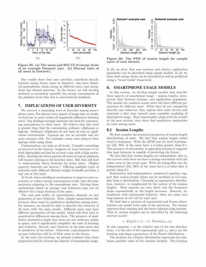
Figure 25(a) shows for an example user that the drain isnot the same throughout the day but has diurnal variationsin which more energy is consumed during the day than dur-ing the night. For this user, the level of energy consumedchanges by roughly a factor of five. Figure 25(b) plots thediurnal ratio of energy use for all users. It shows that diurnalvariations occur, with di!erent strengths, for all users.
2060
100
140
0 4 8 12 16 20Hour of the day
Batte
ry D
rain
(mAh
)
(a)
0 20 40 60 80 100
12
34
56
7
User percentile
Diu
rnal
ratio
(b)
Figure 25: (a) The mean and 95% CI of energy drainof an example Dataset1 user. (b) Diurnal ratio ofall users in Dataset1.
Our results show that user activities contribute heavilytowards energy drain; users in Dataset1, who have identi-cal smartphones, drain energy at di!erent rates, and energydrain has diurnal patterns. In the future, we will developmethods to accurately quantify the energy consumption ofthe platform from that due to user-induced workload.
7. IMPLICATIONS OF USER DIVERSITYWe uncover a surprising level of diversity among smart-
phone users. For almost every aspect of usage that we study,we find one or more orders of magnitude di!erence betweenusers. Our findings strongly motivate the need for customiz-ing smartphones to their users. We believe that this needis greater than that for customizing ordinary cellphones orlaptops. Ordinary cellphones do not have as rich an appli-cation environment. Laptops are not as portable and aremore resource rich. For example, many users plug-in theirlaptops while using them.
Customization can help at all levels. Consider somethingas low-level as the battery. Suppose we want batteries to beboth lightweight and last for at least a day with a high proba-bility. Meeting the latter goal for all users of a given platformwill require catering to the heaviest users. But that will leadto unnecessarily heavy batteries for many users. (Highercapacity batteries are heavier.) O!ering multiple types ofbatteries with di!erent lifetime-weight tradeo!s provides away out of this bind.
At levels where intelligent mechanisms to improve user ex-perience or reduce energy consumption reside, user diversitymotivates adapting to the smartphone user. Driving thesemechanisms based on average case behaviors may not bee!ective for a large fraction of the users.
The ease and utility of customization depends on twoproperties of user behavior. First, despite quantitative dif-ferences, there must be qualitative similarities among users.For instance, we should be able to describe the behavior ofall users with the same model. Di!erent users may havedi!erent parameters of this model, which will then lead toquantitative di!erences among them. The presence of qual-itative similarities imply that users are not arbitrary pointsin space, and it significantly simplifies the task of learninguser behavior. Second, user behavior in the past must alsobe predictive of the future. Otherwise, customization basedon past behaviors will be of little value in the future.
In the next two sections, we present evidence that theseproperties hold for several key aspects of smartphone usage.
Dataset1 example user
0.00
00.
010
0.02
00.
030
0 100 200 300 400Session length (s)
Den
sity
Dataset2 example user
0.00
0.05
0.10
0.15
0.20
0 20 40 60 80 100Session length (s)
Den
sity
Figure 26: The PDF of session length for sampleusers of each dataset.
In §8, we show that user sessions and relative applicationpopularity can be described using simple models. In §9, weshow that energy drain can be described as well as predictedusing a “trend trable” framework.
8. SMARTPHONE USAGE MODELSIn this section, we develop simple models that describe
three aspects of smartphone usage – session lengths, inter-arrival time between sessions, and application popularity.The models are common across users but have di!erent pa-rameters for di!erent users. While they do not completelydescribe user behavior, they capture first order factors andrepresent a first step towards more complete modeling ofsmartphone usage. More importantly, along with the resultsof the next section, they show that qualitative similaritiesdo exist among users.
8.1 Session LengthsWe first consider the statistical properties of session length
distributions of users. We find that session length valuestend to stationary. With the KPSS test for level stationar-ity [13], 90% of the users have a p-value greater than 0.1.The presence of stationarity is appealing because it suggeststhat past behavior is capable of predicting the future.
We also find that session lengths are independent, that is,the current value does not have a strong correlation with thevalues seen in the recent past. With the Ljung-Box test forindependence [15], 96% of the users have a p-value that isgreater than 0.1.
Stationarity and independence, considered together, sug-gest that session length values can be modeled as i.i.d sam-ples from a distribution. Choosing an appropriate distribu-tion, however, is complicated by the nature of the sessionlengths. Most sessions are very short and the frequencydrops exponentially as the length increases. However, in-consistent with exponential behavior, there are some verylong sessions in the tail for each user.
We find that a mixture of exponential and Pareto distri-butions can model both ends of the spectrum. The formercaptures short sessions and the latter captures long sessions.That is, session lengths can be described by the followingmixture model:
r · Exp(!) + (1 ! r) · Pareto(xm, ")
In this equation, r is the relative mix of the two distribu-tions, ! is the rate of the exponential, and xm and " are thelocation and shape parameters of the Pareto distribution.
The location for a Pareto distribution represents the min-imum possible value of the random variable. The location
010
0020
0030
00
0 1000 2000 3000Observed quantiles
Mod
el q
uant
iles
Figure 27: QQ plot of session lengths model for asample user
0.0
0.2
0.4
0.6
0.8
1.0
0 20 40 60 80 100User percentile
Estim
ated
mix
(a) Relative mix (r)
0.0
0.2
0.4
0.6
0.8
1.0
0 20 40 60 80 100User percentile
Estim
ated
rate
(b) Exponential rate (!)
020
4060
0 20 40 60 80 100User percentile
Tim
eout
(s)
(c) Pareto location (xm)
−1.0
−0.4
0.2
0.6
1.0
0 20 40 60 80 100User percentile
Estim
ated
sha
pe
(d) Pareto shape (")
Figure 28: Distribution of inferred model parame-ters that describe session length values of users inboth datasets.
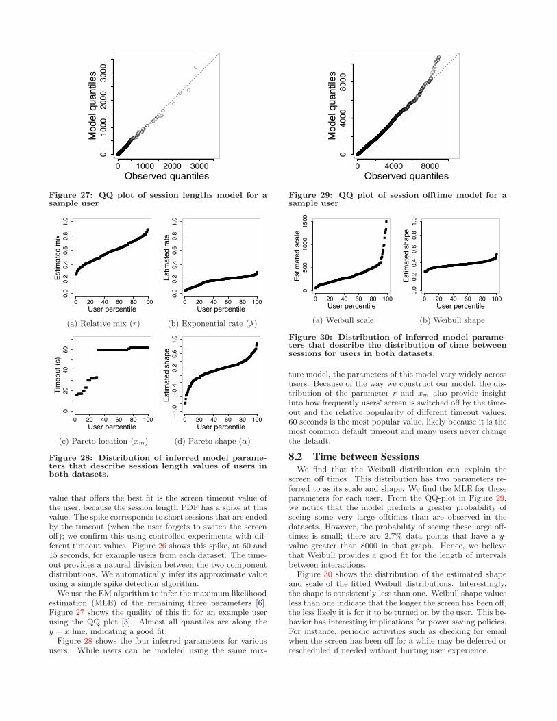
value that o!ers the best fit is the screen timeout value ofthe user, because the session length PDF has a spike at thisvalue. The spike corresponds to short sessions that are endedby the timeout (when the user forgets to switch the screeno!); we confirm this using controlled experiments with dif-ferent timeout values. Figure 26 shows this spike, at 60 and15 seconds, for example users from each dataset. The time-out provides a natural division between the two componentdistributions. We automatically infer its approximate valueusing a simple spike detection algorithm.
We use the EM algorithm to infer the maximum likelihoodestimation (MLE) of the remaining three parameters [6].Figure 27 shows the quality of this fit for an example userusing the QQ plot [3]. Almost all quantiles are along they = x line, indicating a good fit.
Figure 28 shows the four inferred parameters for varioususers. While users can be modeled using the same mix-
040
0080
00
0 4000 8000Observed quantiles
Mod
el q
uant
iles
Figure 29: QQ plot of session o!time model for asample user
050
010
0015
000 20 40 60 80 100
User percentileEs
timat
ed s
cale
(a) Weibull scale
0.0
0.2
0.4
0.6
0.8
1.0
0 20 40 60 80 100User percentile
Estim
ated
sha
pe
(b) Weibull shape
Figure 30: Distribution of inferred model parame-ters that describe the distribution of time betweensessions for users in both datasets.
ture model, the parameters of this model vary widely acrossusers. Because of the way we construct our model, the dis-tribution of the parameter r and xm also provide insightinto how frequently users’ screen is switched o! by the time-out and the relative popularity of di!erent timeout values.60 seconds is the most popular value, likely because it is themost common default timeout and many users never changethe default.
8.2 Time between SessionsWe find that the Weibull distribution can explain the
screen o! times. This distribution has two parameters re-ferred to as its scale and shape. We find the MLE for theseparameters for each user. From the QQ-plot in Figure 29,we notice that the model predicts a greater probability ofseeing some very large o!times than are observed in thedatasets. However, the probability of seeing these large o!-times is small; there are 2.7% data points that have a y-value greater than 8000 in that graph. Hence, we believethat Weibull provides a good fit for the length of intervalsbetween interactions.
Figure 30 shows the distribution of the estimated shapeand scale of the fitted Weibull distributions. Interestingly,the shape is consistently less than one. Weibull shape valuesless than one indicate that the longer the screen has been o!,the less likely it is for it to be turned on by the user. This be-havior has interesting implications for power saving policies.For instance, periodic activities such as checking for emailwhen the screen has been o! for a while may be deferred orrescheduled if needed without hurting user experience.
020
4060
8010
0
0 20 40 60 80 100User percentile
MSE
(%)
(a) MSE
0.0
0.2
0.4
0.6
0.8
1.0
0 20 40 60 80 100User percentile
Estim
ated
rate
(b) Rate parameter
Figure 31: (a) The mean square error (MSE) whenapplication popularity distribution is modeled usingan exponential. (b) The inferred rate parameter ofthe exponential distribution for di!erent users.
8.3 Application PopularityWe find that for each user the relative popularity of ap-
plications can be well described by a simple exponential dis-tribution. This qualitative invariant is useful, for instance,to predict how many applications account for a given frac-tion of user attention. For the example users in Figure 11,this facet can be seen in the inset plots; the semi-log of thepopularity distribution is very close to a straight line.
Figure 31(a) shows that this exponential drop in applica-tion popularity is true for almost all users; the mean squareerror between modeled exponential and actual popularitydistribution is less than 5% for 95% of the users.
Figure 31(b) shows the inferred rate parameter of the ap-plication popularity distribution for various users. We seethat the rate varies by an order of magnitude, from 0.1 toalmost 1. The value of the rate essentially captures the paceof the drop in application popularity. Lower values describeusers that use more applications on a regular basis. Oneimplication of the wide range is that it may be feasible toretain all popular applications in memory for some users andnot for others.
9. PREDICTING ENERGY DRAINIn this section, we demonstrate the value of adapting to
user behaviors in the context of a mechanism to predict fu-ture energy drain on the smartphone. Such a mechanismcan help with scheduling background tasks [9], estimatingbattery lifetime, and improving user experience if it is esti-mated that the user will not fully drain the battery until thenext charging cycle [2, 21].
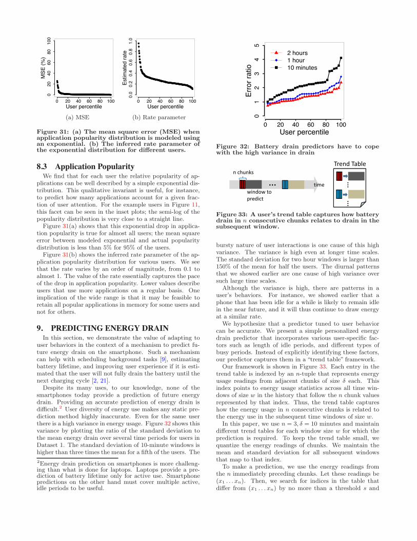
Despite its many uses, to our knowledge, none of thesmartphones today provide a prediction of future energydrain. Providing an accurate prediction of energy drain isdi"cult.2 User diversity of energy use makes any static pre-diction method highly inaccurate. Even for the same userthere is a high variance in energy usage. Figure 32 shows thisvariance by plotting the ratio of the standard deviation tothe mean energy drain over several time periods for users inDataset 1. The standard deviation of 10-minute windows ishigher than three times the mean for a fifth of the users. The
2Energy drain prediction on smartphones is more challeng-ing than what is done for laptops. Laptops provide a pre-diction of battery lifetime only for active use. Smartphonepredictions on the other hand must cover multiple active,idle periods to be useful.
01
23
45
0 20 40 60 80 100User percentile
Erro
r rat
io
2 hours1 hour10 minutes
Figure 32: Battery drain predictors have to copewith the high variance in drain
time window to predict
n chunks
�…
Trend Table
�…
�…
Figure 33: A user’s trend table captures how batterydrain in n consecutive chunks relates to drain in thesubsequent window.
bursty nature of user interactions is one cause of this highvariance. The variance is high even at longer time scales.The standard deviation for two hour windows is larger than150% of the mean for half the users. The diurnal patternsthat we showed earlier are one cause of high variance oversuch large time scales.
Although the variance is high, there are patterns in auser’s behaviors. For instance, we showed earlier that aphone that has been idle for a while is likely to remain idlein the near future, and it will thus continue to draw energyat a similar rate.
We hypothesize that a predictor tuned to user behaviorcan be accurate. We present a simple personalized energydrain predictor that incorporates various user-specific fac-tors such as length of idle periods, and di!erent types ofbusy periods. Instead of explicitly identifying these factors,our predictor captures them in a “trend table” framework.
Our framework is shown in Figure 33. Each entry in thetrend table is indexed by an n-tuple that represents energyusage readings from adjacent chunks of size # each. Thisindex points to energy usage statistics across all time win-dows of size w in the history that follow the n chunk valuesrepresented by that index. Thus, the trend table captureshow the energy usage in n consecutive chunks is related tothe energy use in the subsequent time windows of size w.
In this paper, we use n = 3, # = 10 minutes and maintaindi!erent trend tables for each window size w for which theprediction is required. To keep the trend table small, wequantize the energy readings of chunks. We maintain themean and standard deviation for all subsequent windowsthat map to that index.
To make a prediction, we use the energy readings fromthe n immediately preceding chunks. Let these readings be(x1 . . . xn). Then, we search for indices in the table thatdi!er from (x1 . . . xn) by no more than a threshold s and
GenericShort−termTime−of−dayPersonalized
0.0
0.5
1.0
1.5
0 20 40 60 80 100User percentile
Erro
r rat
io
(a) 1-hour window
0.0
0.5
1.0
1.5
0 20 40 60 80 100User percentile
Erro
r rat
io
GenericShort−termTime−of−dayPersonalized
(b) 2-hour window
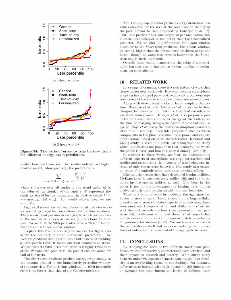
Figure 34: The ratio of error to true battery drainfor di!erent energy drain predictors.
predict based on them, such that similar indices have higherrelative weight. More precisely, the prediction is
X
e s.t.!i=1...n|hei "xi|<s
ke " ue
Pke
,
where e iterates over all tuples in the trend table, hei is
the value of the chunk i of the tuple e, ue represents thestatistics stored for that index, and the relative weight ke =s ! maxi=1...n |he
i ! xi|. For results shown here, we uses = 0.5%.
Figures 34 shows how well our Personalized predictor worksfor predicting usage for two di!erent future time windows.There is one point per user in each graph, which correspondsto the median error seen across many predictions for thatuser. We see that the 90th percentile error is 25% for 1-hourwindow and 40% for 2-hour window.
To place this level of accuracy in context, the figure alsoshows the accurary of three alternative predictors. TheGeneric predictor uses a trend table but instead of buildinga user-specific table, it builds one that combines all users.We see that its 90th percentile error is roughly twice thatof the Personalized predictor. Its predictions are worse forhalf of the users.
The Short-term predictor predicts energy drain simply asthe amount drained in the immediately preceding windowof the same size. For both time windows, its 90th percentileerror is no better than that of the Generic predictor.
The Time-of-day predictor predicts energy drain based onvalues observed for the user at the same time of the day inthe past, similar to that proposed by Banerjee et al. [2].Thus, this predictor has some degree of personalization, butit learns user behavior in less detail than the Personalizedpredictor. We see that its performance for 1-hour windowis similar to the Short-term predictor. For 2-hour window,its error is higher than the Personalized predictor across theboard, though its worst case error is lower than the Short-term and Generic predictors.
Overall, these results demonstrate the value of appropri-ately learning user behaviors to design intelligent mecha-nisms on smartphones.
10. RELATED WORKIn a range of domains, there is a rich history of work that
characterizes user workloads. However, because smartphoneadoption has gathered pace relatively recently, our work rep-resents one of the few to study how people use smartphones.
Along with other recent works, it helps complete the pic-ture. Banerjee et al. and Rahmati et al. report on batterycharging behaviors [2, 18]. Like us, they find considerablevariation among users. Banerjee et al. also propose a pre-dictor that estimates the excess energy of the battery atthe time of charging, using a histogram of past battery us-age [2]. Shye et al. study the power consumption character-istics of 20 users [24]. They infer properties such as whichcomponents in the phone consume most power and exploreoptimizations based on these characteristics. Rahmati andZhong study 14 users of a particular demographic to studywhich applications are popular in that demographic, wherethe phone is used, and how it is shared among users [19].
In contrast to these works, we focus on understandingdi!erent aspects of smartphone use (e.g., interactions andtra"c) and on exposing the diversity of user behaviors, in-stead of only the average behavior. Our study also entailsan order of magnitude more users than previous e!orts.
Like us, other researchers have developed logging utilities.MyExperience is one such early utility [10], and the worksabove involve custom utilities as well. Our focus in thispaper is not on the development of logging tools but onanalyzing their data to gain insight into user behavior.
There is a body of work in modeling the aggregate be-havior of mobile users. Using traces from a large cellularoperator some network related aspects of mobile usage havebeen modeled. Halepovic et al. and Williamson et al. re-port that call arrivals are bursty and present diurnal pat-terns [28]. Willkomm et al. and Brown et al. report thatmobile users call duration can be approximately modeled bya lognormal distribution [4, 29]. We use traces collected onthe mobile device itself and focus on modeling the interac-tions of individual users instead of the aggregate behavior.
11. CONCLUSIONSBy studying 255 users of two di!erent smartphone plat-
forms, we comprehensively characterized user activities andtheir impact on network and battery. We quantify manyhitherto unknown aspects of smartphone usage. User diver-sity is an overarching theme in our findings. For instance,di!erent users interact with their phones 10-200 times a dayon average; the mean interaction length of di!erent users
is 10-250 seconds; and users receive 1-1000 MB of data perday, where 10-90% is received as part of active use.
This extent of user diversity implies that mechanisms thatwork for the average case may be ine!ective for a large frac-tion of the users. Instead, learning and adapting to userbehaviors is likely to be more e!ective, as demonstrated byour personalized energy drain predictor. We show that qual-itative similarities exist among users to facilitate the devel-opment of such mechanisms. For instance, the longer theuser has not interacted with the phone, the less likely it isfor her to start interacting with it; and application popular-ity for a user follows a simple exponential distribution.
Our study points to ways in which smartphone platformsshould be enhanced. E!ective adaptation will require futureplatforms to support light-weight tools that monitor andlearn user behaviors in situ. It will also require them toexpose appropriate knobs to control the behavior of lower-level components (e.g., CPU or radio).
12. ACKNOWLEDGEMENTSWe are grateful to the users in Dataset1 that ran our log-
ger and to the providers of Dataset2. Elizabeth Dawson pro-vided administrative support for data collection. Jean Bolot,Kurt Partridge, Stefan Saroiu, Lin Zhong, and the MobiSysreviewers provided many comments that helped improve thepaper. We thank them all. This work is supported in partby the NSF grants CCR-0120778 and CNS-0627084.
13. REFERENCES[1] Balasubramanian, N., Balasubramanian, A.,
and Venkataramani, A. Energy consumption inmobile phones: A measurement study andimplications for network applications. In IMC (2009).
[2] Banerjee, N., Rahmati, A., Corner, M. D.,Rollins, S., and Zhong, L. Users and batteries:Interactions and adaptive energy management inmobile systems. In Ubicomp (2007).
[3] Becker, R., Chambers, J., and Wilks, A. The newS language. Chapman & Hall/CRC, 1988.
[4] Brown, L., Gans, N., Mandelbaum, A., Sakov,A., Shen, H., Zeltyn, S., and Zhao, L. Statisticalanalysis of a telephone call center. Journal of theAmerican Statistical Association 100, 469 (2005).
[5] Church, K., and Smyth, B. Understanding mobileinformation needs. In MobileHCI (2008).
[6] Dempster, A., Laird, N., and Rubin, D. Maximumlikelihood from incomplete data via the EM algorithm.Journal of the Royal Statistical Society. Series B(Methodological) 39, 1 (1977).
[7] Esfahbod, B. Preload: An adaptive prefetchingdaemon. Master’s thesis, University of Toronto, 2006.
[8] Falaki, H., Govindan, R., and Estrin, D. Smartscreen management on mobile phones. Tech. Rep. 74,Center for Embedded Networked Sesning, 2009.
[9] Flinn, J., and Satyanarayanan, M. Managingbattery lifetime with energy-aware adaptation. ACMTOCS 22, 2 (2004).
[10] Froehlich, J., Chen, M., Consolvo, S.,Harrison, B., and Landay, J. MyExperience: Asystem for in situ tracing and capturing of userfeedback on mobile phones. In MobiSys (2007).
[11] Fukuda, K., Cho, K., and Esaki, H. The impact ofresidential broadband tra"c on Japanese ISPbackbones. SIGCOMM CCR 35, 1 (2005).
[12] Kotz, D., and Essien, K. Analysis of a campus-widewireless network. Wireless Networks 11, 1–2 (2005).
[13] Kwiatkowski, D., Phillips, P., Schmidt, P., andShin, Y. Testing the null hypothesis of stationarityagainst the alternative of a unit root. Journal ofEconometrics 54, 1-3 (1992).
[14] Lahiri, K., Dey, S., Panigrahi, D., andRaghunathan, A. Battery-driven system design: Anew frontier in low power design. In Asia SouthPacific design automation/VLSI Design (2002).
[15] Ljung, G., and Box, G. On a measure of lack of fitin time series models. Biometrika 65, 2 (1978).
[16] Smartphone futures 2009-2014. http://www.portioresearch.com/Smartphone09-14.html.
[17] Rahmati, A., Qian, A., and Zhong, L.Understanding human-battery interaction on mobilephones. In MobileHCI (2007).
[18] Rahmati, A., and Zhong, L. Human–batteryinteraction on mobile phones. Pervasive and MobileComputing 5, 5 (2009).
[19] Rahmati, A., and Zhong, L. A longitudinal study ofnon-voice mobile phone usage by teens from anunderserved urban community. Tech. Rep. 0515-09,Rice University, 2009.
[20] Rao, R., Vrudhula, S., and Rakhmatov, D.Battery modeling for energy aware system design.IEEE Computer 36, 12 (2003).
[21] Ravi, N., Scott, J., Han, L., and Iftode, L.Context-aware battery management for mobilephones. In PerCom (2008).
[22] Sharma, A., Navda, V., Ramjee, R.,Padmanabhan, V., and Belding, E. Cool-Tether:Energy e"cient on-the-fly WiFi hot-spots usingmobile phones. In CoNEXT (2009).
[23] Sharma, C. US wireless data market update - Q32009. http://www.chetansharma.com/usmarketupdateq309.htm.
[24] Shye, A., Sholbrock, B., and G, M. Into the wild:Studying real user activity patterns to guide poweroptimization for mobile architectures. In Micro (2009).
[25] Snol, L. More smartphones than desktop PCs by2011. http://www.pcworld.com/article/171380/more_smartphones_than_desktop%_pcs_by_2011.html.
[26] Sohn, T., Li, K., Griswold, W., and Hollan, J.A diary study of mobile information needs. In SIGCHI(2008).
[27] Trestian, I., Ranjan, S., Kuzmanovic, A., andNucci, A. Measuring serendipity: Connecting people,locations and interests in a mobile 3G network. InIMC (2009).
[28] Williamson, C., Halepovic, E., Sun, H., and Wu,Y. Characterization of CDMA2000 Cellular DataNetwork Tra"c. In Local Computer Networks (2005).
[29] Willkomm, D., Machiraju, S., Bolot, J., andWolisz, A. Primary users in cellular networks: Alarge-scale measurement study. In DySPAN (2008).