EUR 22166 EN/2 - 2008

LISFLOODDistributed Water Balance and Flood

Simulation Model

Johan van der Knijff, Ad de Roo

Revised User Manual

The mission of the Institute for Environment and Sustainability is to provide scientific and technical support to the European Union’s policies for protecting the environment and the EU Strategy for Sustainable Development.

European Commission Directorate-General Joint Research Centre Institute for Environment and Sustainability Contact information Address: Via E. Fermi, TP 261, 21020 Ispra (Va), Italy E-mail: ad.de-roo@jrc.it Tel.: + 39 0332 786 240 Fax: + 39 0332 786 653 http://ies.jrc.cec.eu.int http://www.jrc.cec.eu.int Legal Notice Neither the European Commission nor any person acting on behalf of the Commission is responsible for the use which might be made of this publication.

Europe Direct is a service to help you find answers to your questions about the European Union

Freephone number (*):

00 800 6 7 8 9 10 11

(*) Certain mobile telephone operators do not allow access to 00 800 numbers or these calls may be billed.

A great deal of additional information on the European Union is available on the Internet. It can be accessed through the Europa server http://europa.eu/ JRC 44410 EUR 22166 EN/2 ISSN 1018-5593 Luxembourg: Office for Official Publications of the European Communities © European Communities, 2008 Reproduction is authorised provided the source is acknowledged Printed in Italy

Disclaimer Both the program code and this manual have been carefully inspected before printing. However, no warranties, either expressed or implied, are made concerning the accuracy, completeness, reliability, usability, performance, or fitness for any particular purpose of the information contained in this manual, to the software described in this manual, and to other material supplied in connection therewith. The material is provided "as is". The entire risk as to its quality and performance is with the user.

CONTENTS 1. Introduction ..............................................................................................................1

About LISFLOOD .....................................................................................................1 About this User Manual ............................................................................................1

2. Process descriptions ................................................................................................3 Overview...................................................................................................................3 Treatment of meteorological input variables.............................................................5 Rain and snow..........................................................................................................5 Frost index soil .........................................................................................................6 Interception...............................................................................................................7 Evaporation of intercepted water..............................................................................7 Treatment of built-up areas and water bodies ..........................................................8 Water available for infiltration and direct runoff ........................................................9 Water uptake by plant roots and transpiration........................................................10 Direct evaporation from the soil surface .................................................................11 Infiltration capacity..................................................................................................12 Preferential bypass flow .........................................................................................13 Actual infiltration and surface runoff .......................................................................13 Soil moisture redistribution .....................................................................................13 Groundwater...........................................................................................................15 Routing of surface runoff to channel.......................................................................16 Routing of sub-surface runoff to channel................................................................18 Channel routing ......................................................................................................18 Special simulation options ......................................................................................19

3. Installation of the LISFLOOD model ......................................................................21 System requirements..............................................................................................21 Installation on Windows systems............................................................................21 Installation on Linux systems..................................................................................22 Running the model .................................................................................................22

4. Model setup: input files ..........................................................................................23 Input maps..............................................................................................................23

Map location attributes and distance units..........................................................25 Role of “mask” and “channels” maps ..................................................................26 Naming of meteorological variable maps............................................................26

Input tables .............................................................................................................28 Organisation of input data ......................................................................................28 Generating input base maps ..................................................................................29

5. LISFLOOD setup: the settings file..........................................................................31 Layout of the settings file........................................................................................31

lfuser and and lfbinding elements .......................................................................32 Variables in the lfbinding element .......................................................................35 Variables in the lfuser element............................................................................37 lfoption element...................................................................................................37 Viewing available options....................................................................................38 Defining options ..................................................................................................38

6. Preparing the settings file.......................................................................................41 Time-related constants ...........................................................................................41 Parameters related to evapo(transpi)ration and interception .................................43 Parameters related to snow and frost.....................................................................44 Infiltration parameters.............................................................................................46 Groundwater parameters........................................................................................47 Routing parameters ................................................................................................47 Parameters related to numerics .............................................................................48 File paths ................................................................................................................49

Prefixes of meteo and vegetation related variables................................................50 Initial conditions ......................................................................................................52 Running the model .................................................................................................54 Using options..........................................................................................................55

7. Initialisation of LISFLOOD......................................................................................59 Introduction.............................................................................................................59 An example.............................................................................................................59 Setting up a LISFLOOD run with warm-up period ..................................................60 Initialisation of the lower groundwater zone ...........................................................61 Lower groundwater zone: steady state storage......................................................61 Steady-state storage in practice .............................................................................64

Procedure 1: prior estimate of average recharge ...............................................64 Procedure 2: use pre-run to calculate average recharge....................................65 Checking the lower zone initialisation .................................................................65

Using the ‘end’ maps of a previous run as initial conditions ...................................66 Summary of LISFLOOD initialisation procedure.....................................................67

8. Output generated by LISFLOOD............................................................................69 Default LISFLOOD output ......................................................................................69 Additional output.....................................................................................................70

References.................................................................................................................77 Annex 1: Simulation of reservoirs ..............................................................................79

Introduction.............................................................................................................79 Description of the reservoir routine.........................................................................79 Preparation of input data ........................................................................................80 Preparation of settings file ......................................................................................81 Reservoir output files..............................................................................................82

Annex 2: Inflow hydrograph option.............................................................................85 Introduction.............................................................................................................85 Description of the inflow hydrograph routine ..........................................................85 Using inflow hydrographs .......................................................................................85 Substituting subcatchments with measured inflow hydrographs ............................86

Exclude subcatchments from MaskMap .............................................................87 Make sure your inflow points are where you need them.....................................87

Annex 3: Dynamic wave option..................................................................................89 Introduction.............................................................................................................89 Time step selection.................................................................................................89 Input data................................................................................................................90 Layout of the cross-section parameter table ..........................................................90 Using the dynamic wave.........................................................................................91

Annex 4: Polder option...............................................................................................93 Introduction.............................................................................................................93 Description of the polder routine.............................................................................93 Regulated and unregulated polders .......................................................................94 Preparation of input data ........................................................................................95 Preparation of settings file ......................................................................................96 Polder output files...................................................................................................97 Limitations ..............................................................................................................98

Annex 5: Simulation of lakes......................................................................................99 Introduction.............................................................................................................99 Description of the lake routine ................................................................................99 Initialisation of the lake routine .............................................................................100 Preparation of input data ......................................................................................101 Preparation of settings file ....................................................................................102 Lake output files ...................................................................................................103

Annex 6: Simulation and reporting of water levels ...................................................105 Introduction...........................................................................................................105 Calculation of water levels....................................................................................105 Reporting of water levels ......................................................................................106 Preparation of settings file ....................................................................................106

Annex 7: Simulation and reporting of soil moisture as pF values ............................107 Introduction...........................................................................................................107 Calculation of pF...................................................................................................107 Reporting of pF.....................................................................................................108 Preparation of settings file ....................................................................................108

1

1. Introduction The LISFLOOD model is a hydrological rainfall-runoff model that is capable of simulating the hydrological processes that occur in a catchment. LISFLOOD has been developed by the floods group of the Natural Hazards Project of the Joint Research Centre (JRC) of the European Commission. The specific development objective was to produce a tool that can be used in large and trans-national catchments for a variety of applications, including:

• Flood forecasting • Assessing the effects of river regulation measures • Assessing the effects of land-use change • Assessing the effects of climate change

Although a wide variety of existing hydrological models are available that are suitable for each of these individual tasks, few single models are capable of doing all these jobs. Besides this, our objective requires a model that is spatially distributed and –at least to a certain extent- physically-based. Also, the focus of our work is on European catchments. Since several databases exist that contain pan-European information on soils (King et al., 1997; Wösten et al., 1999), land cover (CEC, 1993), topography (Hiederer & de Roo, 2003) and meteorology (Rijks et al., 1998), it would be advantageous to have a model that makes the best possible use of these data. Finally, the wide scope of our objective implies that changes and extensions to the model will be required from time to time. Therefore, it is essential to have a model code that can be easily maintained and modified. LISFLOOD has been specifically developed to satisfy these requirements. The model is designed to be applied across a wide range of spatial and temporal scales. LISFLOOD is grid-based, and applications so far have employed grid cells of as little as 100 metres for medium-sized catchments, up to 5000 metres for modelling the whole of Europe. Long-term water balance can be simulated (using a daily time step), as well as individual flood events (using hourly time intervals, or even smaller). The output of a “water balance run” can be used to provide the initial conditions of a “flood run”. Although the model’s primary output product is channel discharge, all internal rate and state variables (soil moisture, for example) can be written as output as well. In addition, all output can be written as grids, or time series at user-defined points or areas. The user has complete control over how output is written, thus minimising any waste of disk space or CPU time.

About LISFLOOD The LISFLOOD model is implemented in the PCRaster Environmental Modelling language (Wesseling et al., 1996), wrapped in a Python based interface. PCRaster is a raster GIS environment that has its own high-level computer language, which allows the construction of iterative spatio-temporal environmental models. The Python wrapper of LISFLOOD enables the user to control the model inputs and outputs and the selection of the model modules. This approach combines the power, relative simplicity and maintainability of code written in the the PCRaster Environmental Modelling language and the flexibility of Python. LISFLOOD runs on any operating for which Python and PCRaster are available. Currently these include 32-bits Windows (e.g. Windows XP, Vista) and a number of Linux distributions.

About this User Manual This revised User Manual documents LISFLOOD version March 31 2008, and replaces all previous documentation of the model (e.g. van der Knijff & de Roo, 2006;

2

de Roo et. al., 2003). The scope of this document is to give model users all the information that is needed for successfully using LISFLOOD. Chapter 2 explains the theory behind the model, including all model equations. The remaining chapters cover all practical aspects of working with LISFLOOD. A series of Annexes at the end of this document describe some optional features that can be activated when running the model. Most model users will not need these features (which are disabled by default), and for the sake of clarity we therefore decided to keep their description out of the main text. The current document does not cover the calculation of the potential evapo(transpi)ration rates that are needed as input to the model. A separate pre-processor (LISVAP) exists that calculates these variables from standard (gridded) meteorological observations. LISVAP is documented in a separate volume (van der Knijff, 2006).

3

2. Process descriptions

Overview Figure 2.1 gives an overview of the structure of the LISFLOOD model. Basically, the model is made up of the following components:

• a 2-layer soil water balance sub-model • sub-models for the simulation of groundwater and subsurface flow (using 2

parallel interconnected linear reservoirs) • a sub-model for the routing of surface runoff to the nearest river channel • a sub-model for the routing of channel flow (not shown in the Figure)

The processes that are simulated by the model include snow melt (not shown in the Figure), infiltration, interception of rainfall, leaf drainage, evaporation and water uptake by vegetation, surface runoff, preferential flow (bypass of soil layer), exchange of soil moisture between the two soil layers and drainage to the groundwater, sub-surface and groundwater flow, and flow through river channels. Each of these processes is described in more detail in the following.

4

Figure 2.1 Overview of the LISFLOOD model. P = precipitation; Int = interception; EWint = evaporation of intercepted water; Dint = leaf drainage; ESa = evaporation from soil surface; Ta = transpiration (water uptake by plant roots); INFact = infiltration; Rs = surface runoff; D1,2 = drainage from top- to subsoil; D2,gw = drainage from subsoil to upper groundwater zone; Dpref,gw = preferential flow to upper groundwater zone; Duz,lz = drainage from upper- to lower groundwater zone; Quz = outflow from upper groundwater zone; Ql = outflow from lower groundwater zone; Dloss = loss from lower groundwater zone. Note that snowmelt is not included in the Figure (even though it is simulated by the model).

5

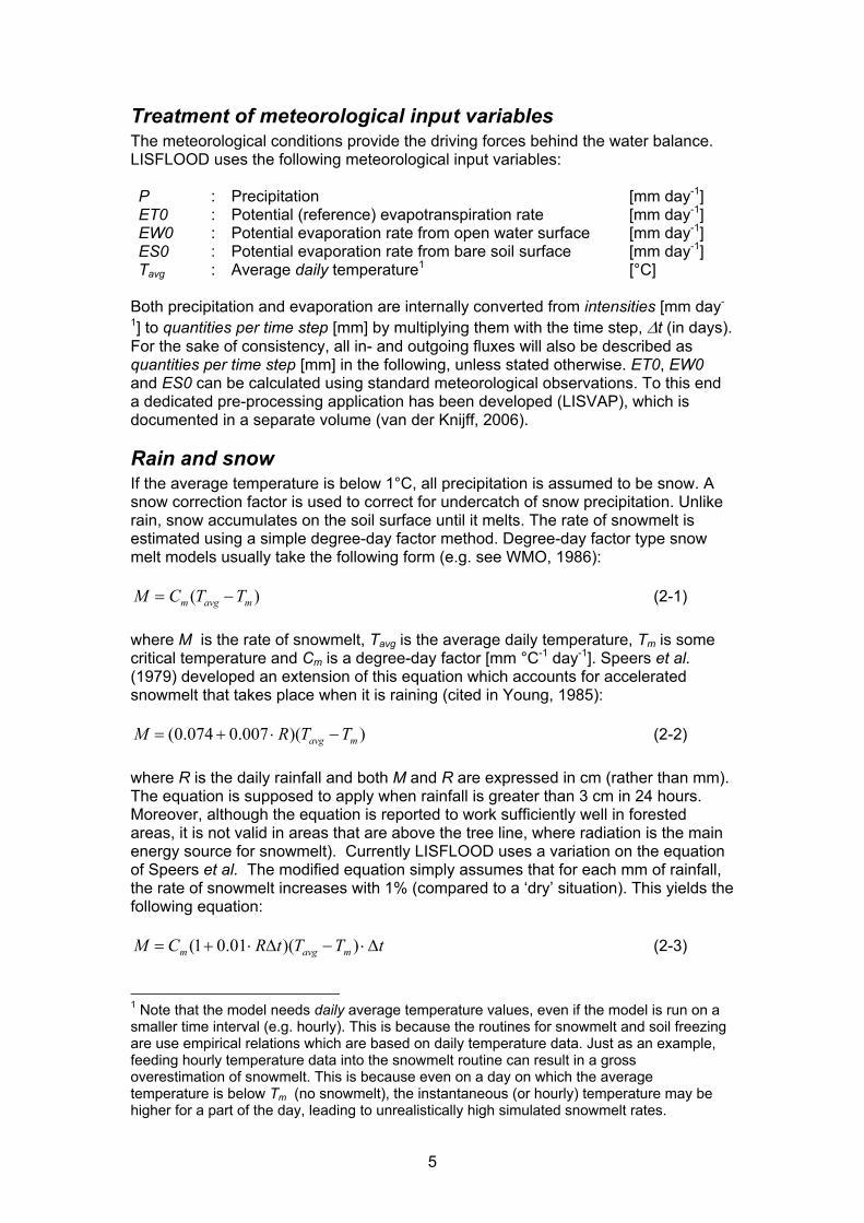
Treatment of meteorological input variables The meteorological conditions provide the driving forces behind the water balance. LISFLOOD uses the following meteorological input variables: P : Precipitation [mm day-1] ET0 : Potential (reference) evapotranspiration rate [mm day-1] EW0 : Potential evaporation rate from open water surface [mm day-1] ES0 : Potential evaporation rate from bare soil surface [mm day-1] Tavg : Average daily temperature1 [°C]

Both precipitation and evaporation are internally converted from intensities [mm day-

1] to quantities per time step [mm] by multiplying them with the time step, Δt (in days). For the sake of consistency, all in- and outgoing fluxes will also be described as quantities per time step [mm] in the following, unless stated otherwise. ET0, EW0 and ES0 can be calculated using standard meteorological observations. To this end a dedicated pre-processing application has been developed (LISVAP), which is documented in a separate volume (van der Knijff, 2006).

Rain and snow If the average temperature is below 1°C, all precipitation is assumed to be snow. A snow correction factor is used to correct for undercatch of snow precipitation. Unlike rain, snow accumulates on the soil surface until it melts. The rate of snowmelt is estimated using a simple degree-day factor method. Degree-day factor type snow melt models usually take the following form (e.g. see WMO, 1986):

)( mavgm TTCM −= (2-1) where M is the rate of snowmelt, Tavg is the average daily temperature, Tm is some critical temperature and Cm is a degree-day factor [mm °C-1 day-1]. Speers et al. (1979) developed an extension of this equation which accounts for accelerated snowmelt that takes place when it is raining (cited in Young, 1985):

))(007.0074.0( mavg TTRM −⋅+= (2-2) where R is the daily rainfall and both M and R are expressed in cm (rather than mm). The equation is supposed to apply when rainfall is greater than 3 cm in 24 hours. Moreover, although the equation is reported to work sufficiently well in forested areas, it is not valid in areas that are above the tree line, where radiation is the main energy source for snowmelt). Currently LISFLOOD uses a variation on the equation of Speers et al. The modified equation simply assumes that for each mm of rainfall, the rate of snowmelt increases with 1% (compared to a ‘dry’ situation). This yields the following equation:

tTTtRCM mavgm Δ⋅−Δ⋅+= ))(01.01( (2-3) 1 Note that the model needs daily average temperature values, even if the model is run on a smaller time interval (e.g. hourly). This is because the routines for snowmelt and soil freezing are use empirical relations which are based on daily temperature data. Just as an example, feeding hourly temperature data into the snowmelt routine can result in a gross overestimation of snowmelt. This is because even on a day on which the average temperature is below Tm (no snowmelt), the instantaneous (or hourly) temperature may be higher for a part of the day, leading to unrealistically high simulated snowmelt rates.

6

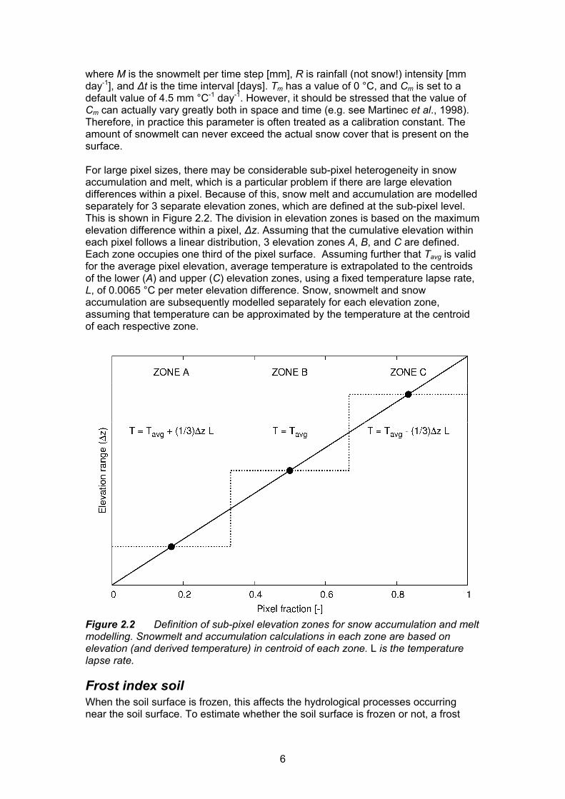
where M is the snowmelt per time step [mm], R is rainfall (not snow!) intensity [mm day-1], and Δt is the time interval [days]. Tm has a value of 0 °C, and Cm is set to a default value of 4.5 mm °C-1 day-1. However, it should be stressed that the value of Cm can actually vary greatly both in space and time (e.g. see Martinec et al., 1998). Therefore, in practice this parameter is often treated as a calibration constant. The amount of snowmelt can never exceed the actual snow cover that is present on the surface. For large pixel sizes, there may be considerable sub-pixel heterogeneity in snow accumulation and melt, which is a particular problem if there are large elevation differences within a pixel. Because of this, snow melt and accumulation are modelled separately for 3 separate elevation zones, which are defined at the sub-pixel level. This is shown in Figure 2.2. The division in elevation zones is based on the maximum elevation difference within a pixel, Δz. Assuming that the cumulative elevation within each pixel follows a linear distribution, 3 elevation zones A, B, and C are defined. Each zone occupies one third of the pixel surface. Assuming further that Tavg is valid for the average pixel elevation, average temperature is extrapolated to the centroids of the lower (A) and upper (C) elevation zones, using a fixed temperature lapse rate, L, of 0.0065 °C per meter elevation difference. Snow, snowmelt and snow accumulation are subsequently modelled separately for each elevation zone, assuming that temperature can be approximated by the temperature at the centroid of each respective zone.

Figure 2.2 Definition of sub-pixel elevation zones for snow accumulation and melt modelling. Snowmelt and accumulation calculations in each zone are based on elevation (and derived temperature) in centroid of each zone. L is the temperature lapse rate.

Frost index soil When the soil surface is frozen, this affects the hydrological processes occurring near the soil surface. To estimate whether the soil surface is frozen or not, a frost

7

index F is calculated. The equation is based on Molnau & Bissell (1983, cited in Maidment 1993), and adjusted for variable time steps. The rate at which the frost index changes is given by:

ss wedKavf eTFA

dtdF /04.0)1( ⋅⋅−⋅−−−= (2-4)

dF/dt is expressed in [°C day-1 day-1 ]. Af is a decay coefficient [day-1], K is a a snow depth reduction coefficient [cm-1], ds is the (pixel-average) depth of the snow cover (expressed as mm equivalent water depth), and wes is a parameter called snow water equivalent, which is the equivalent water depth water of a snow cover (Maidment, 1993). In LISFLOOD, Af and K are set to 0.97 and 0.57 cm-1 respectively, and wes is taken as 0.1, assuming an average snow density of 100 kg/m3 (Maidment, 1993). The soil is considered frozen when the frost index rises above a critical threshold of 56. For each time step the value of F [°C day-1] is updated as:

tdtdFtFtF Δ+−= )1()( (2-5)

F is not allowed to become less than 0.

Interception Interception is estimated using the following storage-based equation (Aston, 1978, Merriam, 1960):

)]/exp(1[ maxmax StRkSInt Δ⋅−−⋅= (2-6) where Int [mm] is the interception per time step, Smax [mm] is the maximum interception, R is the rainfall intensity [mm day-1] and the factor k accounts for the density of the vegetation. Smax is calculated using an empirical equation (Von Hoyningen-Huene, 1981):

⎩⎨⎧

≤=>⋅−⋅+=

]1.0[0]1.0[00575.0498.0935.0

max

2max

LAISLAILAILAIS

(2-7)

where LAI is the average Leaf Area Index [m2 m-2] of each model element (pixel). k is estimated as:

LAIk ⋅= 046.0 (2-8) The value of Int can never exceed the interception storage capacity, which is defined as the difference between Smax and the accumulated amount of water that is stored as interception, Intcum.

Evaporation of intercepted water Evaporation of intercepted water, EWint, occurs at the potential evaporation rate from an open water surface, EW0. The maximum evaporation per time step is proportional to the fraction of vegetated area in each pixel (Supit et al.,1994):

8

tLAIEWEW gb Δ⋅−−⋅= )]exp(1[0max κ (2-9) where EW0 is the potential evaporation rate from an open water surface [mm day-1], and EWmax is in [mm] per time step. Constant κgb is the extinction coefficient for global solar radiation [-]. Since evaporation is limited by the amount of water stored on the leaves, the actual amount of evaporation from the interception store equals:

),min( maxint cumInttEWEW Δ⋅= (2-10) where EWint is the actual evaporation from the interception store [mm] per time step, and EW0 is the potential evaporation rate from an open water surface [mm day-1] It is assumed that on average all water in the interception store (Intcum) will have evaporated or fallen to the soil surface as leaf drainage within one day. Leaf drainage is therefore modelled as a linear reservoir with a time constant (or residence time) of one day, i.e:

tIntD cumΔ⋅=int

int T1

(2-11)

where Dint is the amount of leaf drainage per time step [mm] and Tint is a time constant for the interception store [days], which is set to 1 day.

Treatment of built-up areas and water bodies If (part of) a pixel is made up of built-up areas this will influence that pixel’s water-balance. LISFLOOD’s ‘direct runoff fraction’ parameter (fdr) defines the fraction of a pixel that is impervious. For impervious areas, LISFLOOD assumes that:

1. Any water that reaches the surface is added directly to surface runoff 2. The storage capacity of the soil is zero (i.e. no soil moisture storage in the

direct runoff fraction) 3. There is no groundwater storage

The same assumptions are made for open water bodies (e.g. lakes), which should be included in fdr (large lakes that are in direct connection with major river channels can be modelled using LISFLOOD’s lake option, which is described in Annex 5 of this manual). Unless stated otherwise, the description of all soil- and groundwater-related processes below (evaporation, transpiration, infiltration, preferential flow, soil moisture redistribution and groundwater flow) are valid for the permeable domain of each pixel only. However, if you activate any of LISFLOOD’s options for writing these internal model fluxes to timeseries or maps (described in Chapter 8), the model will report the pixel-average fluxes, which are simply the fluxes as described in this manual, multiplied by the permeable fraction (1- fdr). Figure 2.3 illustrates this, using the water uptake by plant roots as an example.

9

Figure 2.3 Simulation of impermeable areas in LISFLOOD. In this example, water uptake by plant roots (transpiration, Ta ) is only simulated in the permeable fraction of the pixel (1-fdr), whereas it is zero in the direct runoff fraction (fdr). Pixel-average fluxes (which are reported by the model as output) are calculated by multiplying by the permeable fraction.

Water available for infiltration and direct runoff In the permeable fraction of each pixel (1- fdr), the amount of water that is available for infiltration, Wav [mm] equals (Supit et al.,1994):

IntDMtRWav −++Δ= int (2-12) where: R : Rainfall [mm day-1] M : Snow melt [mm] Dint : Leaf drainage [mm] Int : Interception [mm] Δt : time step [days]

Since no infiltration can take place in each pixel’s ‘direct runoff fraction’, direct runoff is calculated as:

avdrd WfR ⋅= (2-13) where Rd is in [mm] per time step. Note here that Wav is valid for the permeable fraction only, whereas Rd is valid for the direct runoff fraction.

10

Water uptake by plant roots and transpiration Water uptake and transpiration by vegetation and direct evaporation from the soil surface are modelled as two separate processes. The approach used here is largely based on Supit et al. (1994) and Supit & Van Der Goot (2000). The maximum transpiration per time step [mm] is given by:

intmax )]exp(1[0 EWtLAIETkT gbcrop −Δ⋅−−⋅⋅= κ (2-14) where ET0 is the potential (reference) evapotranspiration rate [mm day-1], and kcrop is a crop coefficient. kcrop is 1 for most vegetation types, except for some excessively transpiring crops like sugarcane. Note that the energy that has been ‘consumed’ already for the evaporation of intercepted water is simply subtracted here in order to respect the overall energy balance. The actual transpiration rate is reduced when the amount of moisture in the soil is small. In the model, a reduction factor is applied to simulate this effect:

)()(

11

11

wpcrit

wpWS ww

wwr

−−

= (2-15)

where w1 is the amount of moisture in the upper soil layer [mm], wwp1 [mm] is the amount of soil moisture at wilting point (pF 4.2) and wcrit1 [mm] is the amount of moisture below which water uptake is reduced and plants start closing their stomata. The critical amount of soil moisture is calculated as:

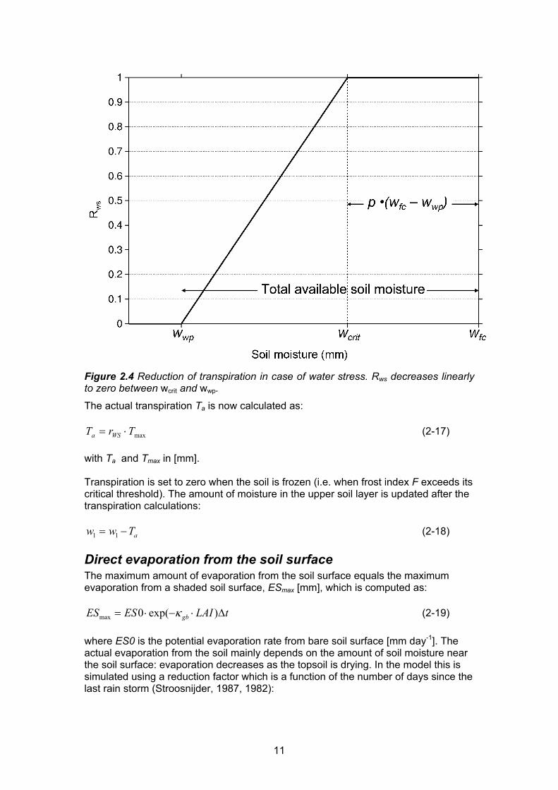
111crit1 )()1( wpwpfc wwwpw +−⋅−= (2-16) where wfc1 [mm] is the amount of soil moisture at field capacity and p is the soil water depletion fraction. RWS varies between 0 and 1: negative values and values greater than 1 are truncated to 0 and 1, respectively. p represents the fraction of soil moisture between wfc1 and wwp1 that can be extracted from the soil without reducing the transpiration rate. Its value is a function of both vegetation type and the potential evapotranspiration rate. The procedure to estimate p is described in detail in Supit & Van Der Goot (2003). Figure 2.4 further illustrates the relation between RWS, w, wcrit, wfc, wwp and p.

11

Figure 2.4 Reduction of transpiration in case of water stress. Rws decreases linearly to zero between wcrit and wwp.

The actual transpiration Ta is now calculated as:

maxTrT WSa ⋅= (2-17) with Ta and Tmax in [mm]. Transpiration is set to zero when the soil is frozen (i.e. when frost index F exceeds its critical threshold). The amount of moisture in the upper soil layer is updated after the transpiration calculations:

aTww −= 11 (2-18)

Direct evaporation from the soil surface The maximum amount of evaporation from the soil surface equals the maximum evaporation from a shaded soil surface, ESmax [mm], which is computed as:

tLAIESES gb Δ⋅−⋅= )exp(0max κ (2-19) where ES0 is the potential evaporation rate from bare soil surface [mm day-1]. The actual evaporation from the soil mainly depends on the amount of soil moisture near the soil surface: evaporation decreases as the topsoil is drying. In the model this is simulated using a reduction factor which is a function of the number of days since the last rain storm (Stroosnijder, 1987, 1982):

12

)1(max −−⋅= slrslra DDESES (2-20) The variable Dslr represents the number of days since the last rain event. Its value accumulates over time: if the amount of water that is available for infiltration (Wav) remains below a critical threshold it increases by an amount of Δt [days] for each time step. It is reset to 1 only if the critical amount of water is exceeded2. The actual soil evaporation is always the smallest value out of the result of the equation above and the available amount of moisture in the soil, i.e.:

),min( 11 resaa wwESES −= (2-21) where w1 [mm] is the amount of moisture in the upper soil layer and wres1 [mm] is the residual amount of soil moisture. Like transpiration, direct evaporation from the soil is set to zero if the soil is frozen. The amount of moisture in the upper soil layer is updated after the evaporation calculations:

aESww −= 11 (2-22)

Infiltration capacity The infiltration capacity of the soil is estimated using the widely-used Xinanjiang (also known as VIC/ARNO) model (e.g. Zhao & Lui, 1995; Todini, 1996). This approach assumes that the fraction of a grid cell that is contributing to surface runoff (read: saturated) is related to the total amount of soil moisture, and that this relationship can be described through a non-linear distribution function. For any grid cell, if w1 is the total moisture storage in the upper soil layer and ws1 is the maximum storage, the corresponding saturated fraction As is approximated by the following distribution function:

b

ss w

wA )1(11

1−−= (2-23)

where ws1 and w1 are the maximum and actual amounts of moisture in the upper soil layer, respectively [mm], and b is an empirical shape parameter. In the LISFLOOD implementation of the Xinanjiang model, As is defined as a fraction of the permeable fraction of each pixel (i.e. as a fraction of (1-drf)). The infiltration capacity INFpot [mm] is a function of ws and As:

])1(1[11

111 b

b

sss

pot Abw

bwINF

+

−−+

−+

= (2-24)

Note that the shape parameter b is related to the heterogeneity within each grid cell. For a totally homogeneous grid cell b approaches zero, which reduces the above equations to a simple ‘overflowing bucket’ model.

2 In the LISFLOOD settings file this critical amount is currently expressed as an intensity [mm day-1]. This is because the equation was originally designed for a daily time step only. Because the current implementation will likely lead to DSLR being reset too frequently, the exact formulation may change in future versions (e.g. by keeping track of the accumulated available water of the last 24 hours).

13

Preferential bypass flow For the simulation of preferential bypass flow –i.e. flow that bypasses the soil matrix and drains directly to the groundwater- no generally accepted equations exist. Because ignoring preferential flow completely will lead to unrealistic model behaviour during extreme rainfall conditions, a very simple approach is used in LISFLOOD. During each time step, a fraction of the water that is available for infiltration is added to the groundwater directly (i.e. without first entering the soil matrix). It is assumed that this fraction is a power function of the relative saturation of the topsoil, which results in an equation that is somewhat similar to the excess soil water equation used in the HBV model (e.g. Lindström et al., 1997):

prefc

savgwpref wwWD )(

1

1, = (2-25)

where Dpref,gw is the amount of preferential flow per time step [mm], Wav is the amount of water that is available for infiltration, and cpref is an empirical shape parameter. fdr is the ‘direct runoff fraction’ [-], which is the fraction of each pixel that is made up by urban area and open water bodies (i.e. preferential flow is only simulated in the permeable fraction of each pixel) . The equation results in a preferential flow component that becomes increasingly important as the soil gets wetter.

Actual infiltration and surface runoff The actual infiltration INFact [mm] is now calculated as:

),min( ,gwprefavpotact DWINFINF −= (2-26) Finally, the surface runoff Rs [mm] is calculated as:

)()1( , actgwprefavdrds INFDWfRR −−⋅−+= (2-27) where Rd is the direct runoff (generated in the pixel’s ‘direct runoff fraction’). If the soil is frozen (F > critical threshold) no infiltration takes place. The amount of moisture in the upper soil layer is updated after the infiltration calculations:

actINFww += 11 (2-28)

Soil moisture redistribution The description of the moisture fluxes out of the subsoil (and also between the upper- and lower soil layer) is based on the simplifying assumption that the flow of soil moisture is entirely gravity-driven. Starting from Darcy’s law for 1-D vertical flow:

]1)()[( −∂

∂−=

zhKq θθ (2-29)

where q [mm day-1] is the flow rate out of the soil (e.g. upper soil layer, lower soil layer); K(θ) [mm day-1] is the hydraulic conductivity (as a function of the volumetric

14

moisture content of the soil, θ [mm3 mm-3]) and zh ∂∂ /)(θ is the matric potential gradient. If we assume a matric potential gradient of zero, the equation reduces to:

)(θKq = (2-30) This implies a flow that is always in downward direction, at a rate that equals the conductivity of the soil. The relationship between hydraulic conductivity and soil moisture status is described by the Van Genuchten equation (van Genuchten, 1980), here re-written in terms of mm water slice, instead of volume fractions:

2/12/1

11)(⎪⎭

⎪⎬⎫

⎪⎩

⎪⎨⎧

⎥⎥⎦

⎤

⎢⎢⎣

⎡⎟⎟⎠

⎞⎜⎜⎝

⎛−−

−−⎟⎟⎠

⎞⎜⎜⎝

⎛−−

=

mm

rs

r

rs

rs ww

wwwwwwKwK (2-31)

where Ks is the saturated conductivity of the soil [mm day-1], and w, wr and ws are the actual, residual and maximum amounts of moisture in the soil respectively (all in [mm]). Parameter m is calculated from the pore-size index, λ (which is related to soil texture):

1+

=λλm (2-32)

For large values of Δt (e.g. 1 day) the above equation often results in amounts of outflow that exceed the available soil moisture storage, i.e:

rwwtwK −>Δ)( (2-33) In order to solve the soil moisture equations correctly an iterative procedure is used. At the beginning of each time step, the conductivities for both soil layers [K1(w1), K2(w2)] are calculated using the Van Genuchten equation. Multiplying these values with the time step and dividing by the available moisture gives a Courant-type numerical stability indicator for each respective layer:

11

111

)(

rwwtwKC

−Δ⋅

= (2-34a)

22

222

)(

rwwtwKC

−Δ⋅

= (2-34b)

A Courant number that is greater than 1 implies that the calculated outflow exceeds the available soil moisture, resulting in loss of mass balance. Since we need a stable solution for both soil layers, the ‘overall’ Courant number for the soil moisture routine is the largest value out of C1 and C2:

),max( 21 CCCsoil = (2-35) In principle, rounding Csoil up to the nearest integer gives the number sub-steps needed for a stable solution. In practice, it is often preferable to use a critical Courant number that is lower than 1, because high values can result in unrealistic ‘jumps’ in the simulated soil moisture pattern when the soil is near saturation (even though mass balance is preserved). Hence, making the critical Courant number a user-defined value Ccrit, the number of sub-steps becomes:

15

)(crit

soil

CCroundupSubSteps = (2-36)

and the corresponding sub-time-step, Δ’t:

SubStepstt Δ

=Δ' (2-37)

In brief, the iterative procedure now involves the following steps. First, the number of sub-steps and the corresponding sub-time-step are computed as explained above. The amounts of soil moisture in the upper and lower layer are copied to temporary variables w’1 and w’2. Two variables, D1,2 (flow from upper to lower soil layer) and D2,gw (flow from lower soil layer to groundwater) are initialized (set to zero). Then, for each sub-step, the following sequence of calculations is performed:

1. compute hydraulic conductivity for both layers 2. compute flux from upper to lower soil layer for this sub-step (D’1,2, can never

exceed storage capacity in lower layer):

]'',)'(min[' 22112,1 wwtwKD s −Δ= (2-38)

3. compute flux from lower soil layer to groundwater for this sub-step (D’2,gw, can never exceed available water in lower layer):

]'',)'(min[' 2222,2 rgw wwtwKD −Δ= (2-39)

4. update w’1 and w’2 5. add D’1,2 to D1,2; add D’2,gw to D2,gw

If the soil is frozen (F > critical threshold), both D1,2 and D2,gw are set to zero. After the iteration loop, the amounts of soil moisture in both layers are updated as follows:

2,111 Dww −= (2-40)

gwDDww ,22,122 −+= (2-41)

Groundwater Groundwater storage and transport are modelled using two parallel linear reservoirs, similar to the approach used in the HBV-96 model (Lindström et al., 1997). The upper zone represents a quick runoff component, which includes fast groundwater and subsurface flow through macro-pores in the soil. The lower zone represents the slow groundwater component that generates the base flow. The outflow from the upper zone to the channel, Quz [mm] equals:

tUZQuz Δ⋅=uzT1

(2-42)

16

where Tuz is a reservoir constant [days] and UZ is the amount of water that is stored in the upper zone [mm. Similarly, the outflow from the lower zone is given by:

tLZQlz Δ⋅=lzT

1 (2-43)

Here, Tlz is again a reservoir constant [days], and LZ is the amount of water that is stored in the lower zone [mm]. The values of both Tuz and Tlz are obtained by calibration. The upper zone also provides the inflow into the lower zone. For each time step, a fixed amount of water percolates from the upper to the lower zone:

),min(, UZtGWD perclzuz Δ⋅= (2-44) Here, GWperc [mm day-1] is a user-defined value that can be used as a calibration constant. For many catchments it is quite reasonable to treat the lower groundwater zone as a system with a closed lower boundary (i.e. water is either stored, or added to the channel). However, in some cases the closed boundary assumption makes it impossible to obtain realistic simulations. Because of this, it is possible to treat of fixed fraction of Qlz as a loss, Dloss, out of the lower zone, i.e.:

lzlossloss QfD ⋅= (2-45) The loss fraction, floss [-], equals 0 for a completely closed lower boundary. If floss is set to 1, all outflow from the lower zone is treated as a loss. Water that flows out of the lower zone through Dloss is quite literally ‘lost’ forever. Physically, the loss term could represent water that is either lost to deep groundwater systems (that do not necessarily follow catchment boundaries), or even groundwater extraction wells. When using the model, it is suggested to use foss with some care; start with a value of zero, and only use any other value if it is impossible to get satisfactory results by adjusting the other calibration parameters. At each time step, the amounts of water in the upper and lower zone are updated for the in- and outgoing fluxes, i.e.:

uzlzuzgwtt QDDUZUZ −−+= − ,,21 (2-46)

lzlzuztt QDLZLZ −+= − ,1 (2-47) Note that these equations are again valid for the permeable fraction of the pixel only: storage in the direct runoff fraction equals 0 for both UZ and LZ.

Routing of surface runoff to channel Surface runoff is routed to the nearest downstream channel using a 4-point implicit finite-difference solution of the kinematic wave equations (Chow, 1988). The basic equations used are the equations of continuity and momentum. The continuity equation is:

srsrsr qtA

xQ

=∂∂

+∂∂

(2-48)

17

where Qsr is the surface runoff [m3 s-1], Asr is the cross-sectional area of the flow [m2] and qsr is the amount of lateral inflow per unit flow length [m2 s-1]. The momentum equation is defined as:

0)( 0 =− fsr SSgAρ (2-49) where ρ is the density of the flow [kg m-3], g is the gravity acceleration [m s-2], S0 is the topographical gradient and Sf is the friction gradient. From the momentum equation it follows that S0= Sf, which means that for the kinematic wave equations it is assumed that the water surface is parallel to the topographical surface. The continuity equation can also be written in the following finite-difference form (please note that for the sake of readability the ‘sr’ subscripts are omitted here from Q, A and q):

21

111

11

111

ji

ji

ji

ji

ji

ji qq

tAA

xQQ +

+++

++

+++ −

=Δ−

+Δ−

(2-50)

where j is a time index and i a space index (such that i=1 for the most upstream cell, i=2 for its downstream neighbour, etcetera). The momentum equation can also be expressed as (Chow et al., 1988):

ksrsrksr QA βα ⋅= , (2-51)

Substituting the right-hand side of this expression in the finite-difference form of the continuity equation gives a nonlinear implicit finite-difference solution of the kinematic wave:

)2

()()( 11

11

111

11

ji

jij

ikji

jik

ji

qqtQQxtQQ

xt

kk +++

+++

+++

+Δ++

ΔΔ

=+ΔΔ ββ αα (2-52)

If αk,sr and βk are known, this non-linear equation can be solved for each pixel and during each time step using an iterative procedure. This numerical solution scheme is available as a built-in function in the PCRaster software. The coefficients αk,sr and βk are calculated by substituting Manning's equation in the right-hand side of Equation 2-51:

535

3

0

32

)( srsr

sr QSPnA ⋅⋅

= (2-53)

where n is Manning's roughness coefficient and Psr is the wetted perimeter of a cross-section of the surface flow. Substituting the right-hand side of this equation for Asr in equation 2-51 gives:

6.0;)( 6.0

0

32

, =⋅

= ksr

srk SPn βα (2-54)

At present, LISFLOOD uses values for αk,sr which are based on a static (reference) flow depth, and a flow width that equals the pixel size, Δx. For each time step, all runoff that is generated (Rs) is added as side-flow (qsr). For each flowpath, the routing stops at the first downstream pixel that is part of the channel network. In other words,

18

the routine only routes the surface runoff to the nearest channel; no runoff through the channel network is simulated at this stage (runoff- and channel routing are completely separated).

Routing of sub-surface runoff to channel All water that flows out of the upper- and lower groundwater zone is routed to the nearest downstream channel pixel within one time step. Recalling once more that the groundwater equations are valid for the pixel’s permeable fraction only, the contribution of each pixel to the nearest channel is made up of (1-fdr)·Quz and (1-fdr)· (Qlz-Dloss), respectively. Figure 3 illustrates the routing procedure: for each pixel that contains a river channel, its contributing pixels are defined by the drainage network. For every 'river pixel' the groundwater outflow that is generated by its upstream pixels is simply summed. For instance, there are two flow paths that are contributing to the second 'river pixel' from the left in Figure 2.5. Hence, the amount of water that is transported to this pixel equals the sum of the amounts of water produced by these flowpaths, q1 + q2. Note that, as with the surface runoff routing, no water is routed through the river network at this stage.

Figure 2.5 Routing of groundwater to channel network. Groundwater flow is routed to the nearest ‘channel’ pixel.

Channel routing Flow through the channel is simulated using the kinematic wave equations. The basic equations and the numerical solution are identical to those used for the surface runoff routing:

chchch qtA

xQ

=∂∂

+∂∂

(2-55)

where Qch is the channel discharge [m3 s-1], Ach is the cross-sectional area of the flow [m2] and qch is the amount of lateral inflow per unit flow length [m2 s-1]. The momentum equation then becomes:

19

0)( 0 =− fch SSgAρ (2-56) where S0 now equals the gradient of the channel bed, and S0= Sf. As with the surface runoff, values for parameter αk,ch are estimated using Manning’s equation:

6.0;)( 6.0

0

32

, =⋅

= kch

chk SPn βα (2-57)

At present, LISFLOOD uses values for αk,ch which are based on a static (reference) channel flow depth (half bankfull) and measured channel dimensions. The term qch (sideflow) now represents the runoff that enters the channel per unit channel length:

∑ ∑ ∑ ++++= chresinlzuzsrch LQQQQQq /)( (2-58) Here, Qsr, Quz and Qlz denote the contributions of surface runoff, outflow from the upper zone and outflow from the lower zone, respectively. Qin is the inflow from an external inflow hydrograph; by default its value is 0, unless the ‘inflow hydrograph’ option is activated (see Annex 2). Qres is the water that flows out of a reservoir into the channel; by default its value is 0, unless the ‘reservoir’ option is activated (see Annex 1). Qsr, Quz, Qlz, Qin and Qres are all expressed in [m3] per time step. Lch is the channel length [m], which may exceed the pixel size (Δx) in case of meandering channels. The kinematic wave channel routing can be run using a smaller time-step than the over simulation timestep, Δt, if needed.

Special simulation options The above model description covers the processes that are simulated in a ‘standard’ LISFLOOD run. By default, special structures in the river channel such as (natural) lakes and regulated reservoirs are not taken into account. However, LISFLOOD has some optional features to model these structures. The description of these features can be found in a series of Annexes at the end of this manual.

20

21

3. Installation of the LISFLOOD model

System requirements Currently LISFLOOD is available on both Linux and 32-bit Windows systems. Either way, the model requires that a recent version of the PCRaster software is available, or at least PCRaster’s ‘pcrcalc’ application and all associated libraries. LISFLOOD versions October 3 2007 and later require ‘pcrcalc’ version October 2, 2007, or more recent. Older ‘pcrcalc’ versions will either not work at all, or they might produce erroneous results. Unless you are using a ‘sealed’ version of LISFLOOD (i.e. a version in which the source code is made unreadable), you will also need a licensed version of ‘pcrcalc’. For details on how to install PCRaster we refer to the PCRaster documentation.

Installation on Windows systems For Windows users the installation involves two steps: 1. Unzip the contents of ‘lisflood_win32.zip’ to an empty folder on your PC (e.g.

‘lisflood’) 2. Open the file ‘config.xml’ in a text editor. This file contains the full path to all files

and applications that are used by LISFLOOD. The items in the file are: • Pcrcalc application : this is the name of the pcrcalc application, including the

full path • LISFLOOD Master Code (optional). This item is usually omitted, and

LISFLOOD assumes that the master code is called ‘lisflood.xml’, and that it is located in the root of the ‘lisflood’ directory (i.e. the directory that contains ‘lisflood.exe’ and all libraries). If –for whatever reason- you want to overrule this behaviour, you can add a ‘mastercode’ element, e.g.:

<mastercode>d:\Lisflood\beta\mastercode\lisflood.xml</mastercode>

The configuration file should look something like this: <?xml version="1.0" encoding="ISO-8859-1"?> <!-- Lisflood configuration file, JvdK, 8 July 2004 --> <!-- !! This file MUST be in the same directory as lisflood.exe --> <!-- (or lisflood) !!! --> <lfconfig> <!-- location of pcrcalc application --> <pcrcalcapp>C:\pcraster\apps\pcrcalc.exe</pcrcalcapp> </lfconfig>

The lisflood executable is a command-line application which can be called from the command prompt (‘DOS’ prompt). To make life easier you may include the full path to ‘lisflood.exe’ in the ’Path’ environment variable. In Windows XP you can do this by selecting ‘settings’ from the ‘Start’ menu; then go to ‘control panel’/’system’ and go to the ‘advanced’ tab. Click on the ‘environment variables’ button. Finally, locate the

22

‘Path’ variable in the ‘system variables’ window and click on ‘Edit’ (this requires local Administrator privileges).

Installation on Linux systems Under Linux LISFLOOD requires that the Python interpreter (version 2.4 or more recent) is installed on the system. Most Linux distributions already have Python pre-installed. If needed you can download Python free of any charge from the following location: http://www.python.org/ The installation process is largely identical to the Windows procedure: unzip the contents of ‘lisflood_llinux.zip’ to an empty directory. Check if the file ‘lisflood’ is executable. If not, make it executable using: chmod 755 lisflood Then update the paths in the configuration file. The configuration file will look something like this: <?xml version="1.0" encoding="ISO-8859-1"?> <!-- Lisflood configuration file, JvdK, 8 July 2004 --> <!-- !! This file MUST be in the same directory as lisflood.exe --> <!-- (or lisflood) !!! --> <lfconfig> <!-- location of pcrcalc application --> <pcrcalcapp>/usr/local/PCRBeta/linux/pcrcalc</pcrcalcapp> </lfconfig>

Running the model Type ‘lisflood’ at the command prompt. You should see something like this: LISFLOOD version March 24 2008 Water balance and flood simulation model for large catchments (C) Institute for Environment and Sustainability Joint Research Centre of the European Commission TP261, I-21020 Ispra (Va), Italy usage (1): lisflood [switches] <InputFile> usage (2): lisflood --listoptions (show options only) InputFile : LISFLOOD input file (see documentation for description of format) switches: -s : keep temporary script after simulation

You can run LISFLOOD by typing ‘lisflood’ followed by a specially-formatted settings file. The layout of this file is described in Chapters 4 and 5. Chapter 3 explains all other input files.

23

4. Model setup: input files In the current version of LISFLOOD, all model input is provided as either maps (grid files in PCRaster format) or tables. This chapter describes all the data that are required to run the model. Files that are specific to optional LISFLOOD features (e.g. inflow hydrographs, reservoirs) are not listed here; they are described in the documentation for each option.

Input maps All input maps roughly fall into any of the following six categories:

• maps related to topography • maps related to soil • maps related to land use • maps related to channel geometry • maps related to the meteorological conditions • maps related to the development of vegetation over time • maps that define at which locations output is generated as time series

All maps that are needed to run the model are listed in the following table3:

3 The file names listed in the table are not obligatory. However, it is suggested to stick to the default names suggested in the table. This will make both setting up the model for new catchments as well as upgrading to possible future LISFLOOD versions much easier.

24

Table 4.1 LISFLOOD input maps (continued on next page)

GENERAL Map Default name Description MaskMap area.map Boolean map that defines model boundaries

TOPOGRAPHY Map Default name Description Ldd ldd.map local drain direction map (with value 1-9); this file

contains flow directions from each cell to its steepest downslope neighbour. Ldd directions are coded according to the following diagram:

This resembles the numeric key pad of your PC’s keyboard, except for the value 5, which defines a cell without local drain direction (pit). The pit cell at the end of the path is the outlet point of a catchment

Grad gradient.map Slope gradient [m m-1], i.e. value of 0.5 indicates a 26.5 degree angle (gradient equals tangent of slope in degrees)

ElevationRange elvrange.map Elevation range, i.e. difference between maximum and minimum elevation within pixel [m]

LAND USE Map Default name Description LandUse landuse.map Map with land use classes (CORINE land cover,

CEC 1993) Forest forest.map Forest fraction for each cell. Values range from 0

(no forest at all) to 1 (pixel is 100% forest) DirectRunoffFraction directrf.map Fraction urban area for each cell. Values range

from 0 (no urban area at all) to 1 (pixel is 100% urban) SOIL

Map Default name Description Texture1 soiltex1.map Soil texture class layer 1 (upper layer) Texture2 soiltex2.map Soil texture class layer 2 (lower layer) SoilDepth soildep.map Soil depth [cm]: depth to bedrock or groundwater

25

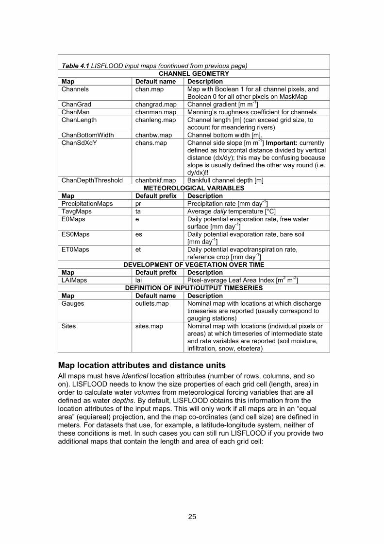
Table 4.1 LISFLOOD input maps (continued from previous page)

CHANNEL GEOMETRY Map Default name Description Channels chan.map Map with Boolean 1 for all channel pixels, and

Boolean 0 for all other pixels on MaskMap ChanGrad changrad.map Channel gradient [m m-1] ChanMan chanman.map Manning’s roughness coefficient for channels ChanLength chanleng.map Channel length [m] (can exceed grid size, to

account for meandering rivers) ChanBottomWidth chanbw.map Channel bottom width [m]. ChanSdXdY chans.map Channel side slope [m m-1] Important: currently

defined as horizontal distance divided by vertical distance (dx/dy); this may be confusing because slope is usually defined the other way round (i.e. dy/dx)!!

ChanDepthThreshold chanbnkf.map Bankfull channel depth [m] METEOROLOGICAL VARIABLES

Map Default prefix Description PrecipitationMaps pr Precipitation rate [mm day-1] TavgMaps ta Average daily temperature [°C] E0Maps e Daily potential evaporation rate, free water

surface [mm day-1] ES0Maps es Daily potential evaporation rate, bare soil

[mm day-1] ET0Maps et Daily potential evapotranspiration rate,

reference crop [mm day-1] DEVELOPMENT OF VEGETATION OVER TIME

Map Default prefix Description LAIMaps lai Pixel-average Leaf Area Index [m2 m-2]

DEFINITION OF INPUT/OUTPUT TIMESERIES Map Default name Description Gauges outlets.map Nominal map with locations at which discharge

timeseries are reported (usually correspond to gauging stations)

Sites sites.map Nominal map with locations (individual pixels or areas) at which timeseries of intermediate state and rate variables are reported (soil moisture, infiltration, snow, etcetera)

Map location attributes and distance units All maps must have identical location attributes (number of rows, columns, and so on). LISFLOOD needs to know the size properties of each grid cell (length, area) in order to calculate water volumes from meteorological forcing variables that are all defined as water depths. By default, LISFLOOD obtains this information from the location attributes of the input maps. This will only work if all maps are in an “equal area” (equiareal) projection, and the map co-ordinates (and cell size) are defined in meters. For datasets that use, for example, a latitude-longitude system, neither of these conditions is met. In such cases you can still run LISFLOOD if you provide two additional maps that contain the length and area of each grid cell:

26

Table 4.2 Optional maps that define grid size

Map Default name Description PixelLengthUser pixleng.map Map with pixel length [m] PixelAreaUser pixarea.map Map with pixel area [m2]

Both maps should be stored in the same directory where all other input maps are. The values on both maps may vary in space. A limitation is that a pixel is always represented as a square, so length and width are considered equal (no rectangles). In order to tell LISFLOOD to ignore the default location attributes and use the maps instead, you need to activate the special option “gridSizeUserDefined”, which involves adding the following line to the LISFLOOD settings file: <setoption choice="1" name="gridSizeUserDefined" /> LISFLOOD settings files and the use of options are explained in detail in Chapter 5 of this document.

Role of “mask” and “channels” maps The mask map (i.e. “area.map”) defines the model domain. In order to avoid unexpected results, it is vital that all maps that are related to topography, land use and soil are defined (i.e. don’t contain a missing value) for each pixel that is “true” (has a Boolean 1 value) on the mask map. The same applies for all meteorological input and the Leaf Area Index maps. Similarly, all pixels that are “true” on the channels map must have some valid (non-missing) value on each of the channel parameter maps. Undefined pixels can lead to unexpected behaviour of the model, output that is full of missing values, loss of mass balance and possibly even model crashes.

Naming of meteorological variable maps The meteorological forcing variables (and Leaf Area Index) are defined in map stacks. A map stack is simply a series of maps, where each map represents the value of a variable at an individual time step. The name of each map is made up of a total of 11 characters: 8 characters, a dot and a 3-character suffix. Each map name starts with a prefix, and ends with the time step number. All character positions in between are filled with zeros (“0”). Take for example a stack of precipitation maps. Table 4.1 shows that the default prefix for precipitation is “pr”, which produces the following file names: pr000000.007 : at time step 7 pr000035.260 : at time step 35260

LISFLOOD can handle two types of stacks. First, there are regular stacks, in which a map is defined for each time step. For instance, the following 10-step stack is a regular stack:

27

t map name 1 pr000000.0012 pr000000.0023 pr000000.0034 pr000000.0045 pr000000.0056 pr000000.0067 pr000000.0078 pr000000.0089 pr000000.00910 pr000000.010

In addition to regular stacks, it is also possible to define sparse stacks. A sparse stack is a stack in which maps are not defined for all time steps, for instance:

t map name 1 pr000000.0012 - 3 - 4 pr000000.0045 - 6 - 7 pr000000.0078 - 9 - 10 -

Here, maps are defined only for time steps 1, 4 and 7. In this case, LISFLOOD will use the map values of pr000000.001 during time steps 1, 2 and 3, those of pr000000.004 during time steps 4, 5 and 6, and those of pr000000.007 during time steps 7, 8, 9 and 10. Since both regular and sparse stacks can be combined within one single run, sparse stacks can be very useful to save disk space. For instance, LISFLOOD always needs the average daily temperature, even when the model is run on an hourly time step. So, instead of defining 24 identical maps for each hour, you can simply define 1 for the first hour of each day and leave out the rest, for instance:

t map name 1 ta000000.0012 - : : : : 25 ta000000.025: : : : 49 ta000000.049: :

Similarly, potential evapo(transpi)ration is usually calculated on a daily basis. So for hourly model runs it is often convenient to define E0, ES0 and ET0 in sparse stacks as well. Leaf Area Index (LAI) is a variable that changes relatively slowly over time, and as a result it is usually advantageous to define LAI in a sparse map stack.

28

Input tables In addition to the maps and time series above, a number of model parameters are read through tables that are linked to the classes on the land use and soil (texture) maps. The following table gives a complete overview: Table 4.3 LISFLOOD input tables

LAND USE Table Default name Description TabCropCoef cropcoef.txt Crop coefficient for each land use class [-] TabCropGroupNumber cropgrpn.txt Crop group number for each land use class TabRootDepth rootdep.txt Rooting depth for each land use class [cm] TabN n.txt Manning’s roughness for each land use class

[-] SOIL TEXTURE

Table Default name Description TabThetaSat1 thetas1.txt Saturated volumetric soil moisture content

layer 1 [-] TabThetaSat2 thetas2.txt Saturated volumetric soil moisture content

layer 2 [-] TabThetaRes1 thetar1.txt Residual volumetric soil moisture content layer

1 [-] TabThetaRes2 thetar2.txt Residual volumetric soil moisture content layer

2 [-] TabLambda1 lambda1.txt Pore size index (λ) layer 1 [-] TabLambda2 lambda2.txt Pore size index (λ) layer 2 [-] TabGenuAlpha1 alpha1.txt Van Genuchten parameter α layer 1 [-] TabGenuAlpha2 alpha2.txt Van Genuchten parameter α layer 2 [-] TabKSat1 ksat1.txt Saturated conductivity layer 1 [cm day-1] TabKSat2 ksat2.txt Saturated conductivity layer 2 [cm day-1]

Organisation of input data It is up to the user how the input data are organised. However, it is advised to keep the base maps, meteorological maps and tables separated (i.e. store them in separate directories). For practical reasons the following input structure is suggested:

• all base maps are in one directory (e.g. ‘maps’) • all tables are in one directory (e.g. ‘tables’) • all meteorological input maps are in one directory (e.g. ‘meteo’) • all Leaf Area Index maps are in one directory (e.g. ‘lai’) • all output goes to one directory (e.g. ‘out’)

The following Figure illustrates this:

29

Figure 4.1 Suggested file structure for LISFLOOD

Generating input base maps At the time of writing this document, complete sets of LISFLOOD base maps covering the whole of Europe have been compiled at 1- and 5-km pixel resolution. A number of automated procedures have been written that allow you to generate sub-sets of these for pre-defined areas (using either existing mask maps or co-ordinates of catchment outlets). These procedures (which are specific to the data server setup at the Floods Action, IES, JRC, Ispra) are documented in a separate document on ‘LISFLOOD and LISVAP map extraction’. If you are an external user of LISFLOOD, please contact the Floods Action to extract the data for you.

30

31

5. LISFLOOD setup: the settings file In LISFLOOD, all file and parameter specifications are defined in a settings file. The purpose of the settings file is to link variables and parameters in the model to in- and output files (maps, time series, tables) and numerical values. In addition, the settings file can be used to specify several options. The settings file has a special (XML) structure. In the next sections the general layout of the settings file is explained. Although the file layout is not particularly complex, a basic understanding of the general principles explained here is essential for doing any successful model runs. The settings file has an XML (‘Extensible Markup Language’) structure. You can edit it using any text editor (e.g. Notepad, Editpad, Emacs, vi). Alternatively, you can also use a dedicated XML editor such as XMLSpy.

Layout of the settings file A LISFLOOD settings file is made up of 4 elements, each of which has a specific function. The general structure of the file is described using XML-tags. XML stands for ‘Extensible Markup Language’, and it is really nothing more than a way to describe data in a file. It works by putting information that goes into a (text) file between tags, and this makes it very easy add structure. For a LISFLOOD settings file, the basic structure looks like this: <lfsettings> Start of settings element <lfuser> Start of element with user-defined variables </lfuser> End of element with user-defined variables <lfoptions> Start of element with options </lfoptions> End of element with options <lfbinding> Start of element with ‘binding’ variables </lfbinding> End of element with ‘binding’ variables <prolog> Start of prolog </prolog> End of prolog <lfsettings> End of settings element

From this you can see the following things:

• The settings file is made up of the elements ‘lfuser’, ‘lfoptions’ and ‘lfbinding’; in addition, there is a ‘prolog’ element (but this will ultimately disappear in future LISFLOOD versions)

• The start of each element is indicated by the element’s name wrapped in square brackets, e.g. <element>

• The end of each element is indicated by a forward slash followed by the element’s name, all wrapped in square brackets, e.g. </element>

32

• All elements are part of a ‘root’ element called ‘<lfsettings>’. In brief, the main function of each element is: lfuser : definition of paths to all in- and output files, and main model

parameters (calibration + time-related) lfbinding : definition of all individual in- and output files, and model parameters lfoptions : switches to turn specific components of the model on or off

The following sections explain the function of each element in more detail. This is mainly to illustrate the main concepts and how it all fits together. A detailed description of all the variables that are relevant for setting up and running LISFLOOD is given in Chapter 6.

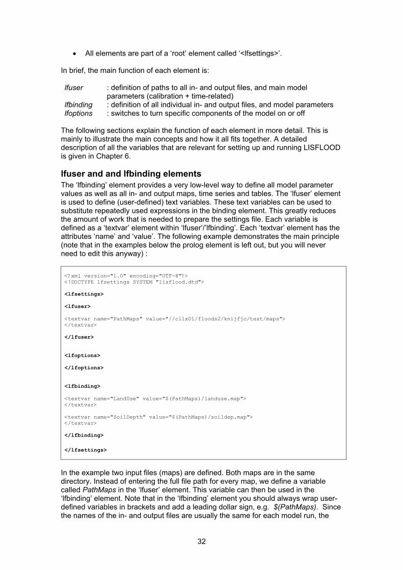
lfuser and and lfbinding elements The ‘lfbinding’ element provides a very low-level way to define all model parameter values as well as all in- and output maps, time series and tables. The ‘lfuser’ element is used to define (user-defined) text variables. These text variables can be used to substitute repeatedly used expressions in the binding element. This greatly reduces the amount of work that is needed to prepare the settings file. Each variable is defined as a ‘textvar’ element within ‘lfuser’/’lfbinding’. Each ‘textvar’ element has the attributes ‘name’ and ‘value’. The following example demonstrates the main principle (note that in the examples below the prolog element is left out, but you will never need to edit this anyway) : <?xml version="1.0" encoding="UTF-8"?> <!DOCTYPE lfsettings SYSTEM "lisflood.dtd"> <lfsettings> <lfuser> <textvar name="PathMaps" value="//cllx01/floods2/knijfjo/test/maps"> </textvar> </lfuser> <lfoptions> </lfoptions> <lfbinding> <textvar name="LandUse" value="$(PathMaps)/landuse.map"> </textvar> <textvar name="SoilDepth" value="$(PathMaps)/soildep.map"> </textvar> </lfbinding>

</lfsettings>

In the example two input files (maps) are defined. Both maps are in the same directory. Instead of entering the full file path for every map, we define a variable called PathMaps in the ‘lfuser’ element. This variable can then be used in the ‘lfbinding’ element. Note that in the ‘lfbinding’ element you should always wrap user-defined variables in brackets and add a leading dollar sign, e.g. $(PathMaps). Since the names of the in- and output files are usually the same for each model run, the

33

use of user-defined variables greatly simplifies setting up the model for new catchments. In general, it is a good idea to use user-defined variables for everything that needs to be changed on a regular basis (paths to input maps, tables, meteorological data, parameter values). This way you only have to deal with the variables in the ‘lfuser’ element, without having to worry about anything in ‘lfbinding’ at all. Now for a somewhat more realistic example:

34

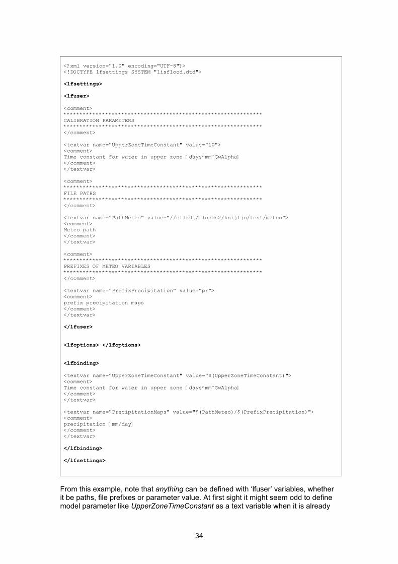
<?xml version="1.0" encoding="UTF-8"?> <!DOCTYPE lfsettings SYSTEM "lisflood.dtd"> <lfsettings> <lfuser> <comment> ************************************************************** CALIBRATION PARAMETERS ************************************************************** </comment> <textvar name="UpperZoneTimeConstant" value="10"> <comment> Time constant for water in upper zone [days*mm^GwAlpha] </comment> </textvar> <comment> ************************************************************** FILE PATHS ************************************************************** </comment> <textvar name="PathMeteo" value="//cllx01/floods2/knijfjo/test/meteo"> <comment> Meteo path </comment> </textvar> <comment> ************************************************************** PREFIXES OF METEO VARIABLES ************************************************************** </comment> <textvar name="PrefixPrecipitation" value="pr"> <comment> prefix precipitation maps </comment> </textvar> </lfuser> <lfoptions> </lfoptions> <lfbinding> <textvar name="UpperZoneTimeConstant" value="$(UpperZoneTimeConstant)"> <comment> Time constant for water in upper zone [days*mm^GwAlpha] </comment> </textvar> <textvar name="PrecipitationMaps" value="$(PathMeteo)/$(PrefixPrecipitation)"> <comment> precipitation [mm/day] </comment> </textvar> </lfbinding> </lfsettings>

From this example, note that anything can be defined with ‘lfuser’ variables, whether it be paths, file prefixes or parameter value. At first sight it might seem odd to define model parameter like UpperZoneTimeConstant as a text variable when it is already

35

defined in the ‘lfbinding’ element. However, in practice it is much easier to have all the important variables defined in the same element: in total the model needs around 200 variables, parameters and file names. By specifying each of those in the ‘lfbinding’ element you need to specify each of them separately. Using the ‘lfuser’ variables this can be reduced to about 50, which greatly simplifies things. You should think of the ‘lfbinding’ element as a low-level way of describing the model in- and output structure: anything can be changed and any file can be in any given location, but the price to pay for this flexibility is that the definition of the input structure will take a lot of work. By using the ‘lfuser’ variables in a smart way, custom template settings files can be created for specific model applications (calibration, scenario modelling, operational flood forecasting). Typically, each of these applications requires its own input structure, and you can use the ‘lfuser’ variables to define this structure. Also, note that the both the name and value of each variable must be wrapped in (single or double) quotes. Dedicated XML-editors like XmlSpy take care of this automatically, so you won’t usually have to worry about this. NOTES:

1. It is important to remember that the only function of the ‘lfuser’ element is to define text variables; you can not use any of these text variables within the ‘lfuser’ element. For example, the following ‘lfuser’ element is wrong and will not work: <lfuser> <textvar name="PathInit" value="//cllx01/floods2/knijfjo/test/init"> <comment> Path to initial conditions maps </comment> </textvar> <textvar name="LZInit" value="$(PathInit)/lzInit.map)"> <comment> Initial lower zone storage ** USE OF USER VARIABLE WITHIN LFUSER ** IS NOT ALLOWED, SO THIS EXAMPLE WILL NOT WORK!! </comment> </textvar> </lfuser>

2. It is possible to define everything directly in the ‘lfbinding’ element without using any text variables at all! In that case the ‘lfuser’ element can remain empty, even though it has to be present (i.e. <lfuser> </lfuser>). In general this is not recommended.

3. Within the lfuser and lfbinding elements, model variables are organised into groups. This is just to make navigation in an xml editor easier.

Variables in the lfbinding element The variables that are defined in the ‘lfbinding’ element fall in either of the following categories:

1. Single map Example:

36

<textvar name="LandUse" value="$(PathMaps)/landuse.map"> <comment> Land Use Classes </comment> </textvar> 2. Table Example:

<textvar name="TabKSat1" value="$(PathTables)/ksat1.txt"> <comment> Saturated conductivity [cm/day] </comment> </textvar> 3. Stack of maps Example:

<textvar name="PrecipitationMaps" value="$(PathMeteo)/$(PrefixPrecipitation)"> <comment> precipitation [mm/day] </comment> </textvar>

Note:

Taking -as an example- a prefix that equals “pr”, the name of each map in the stack starts with “pr”, and ends with the number of the time step. The name of each map is made up of a total of 11 characters: 8 characters, a dot and a 3-character suffix. For instance:

pr000000.007 : at time step 7 pr000035.260 : at time step 35260

To avoid unexpected behaviour, do not use numbers in the prefix! For example:

<textvar name="PrecipitationMaps" value="$(PathMeteo)/pr10 "> <comment> precipitation [mm/day] </comment> </textvar>

For the first time step this yields the following file name: pr100000.001

But this is actually interpreted as time step 100,000,001!

4. Time series file Example:

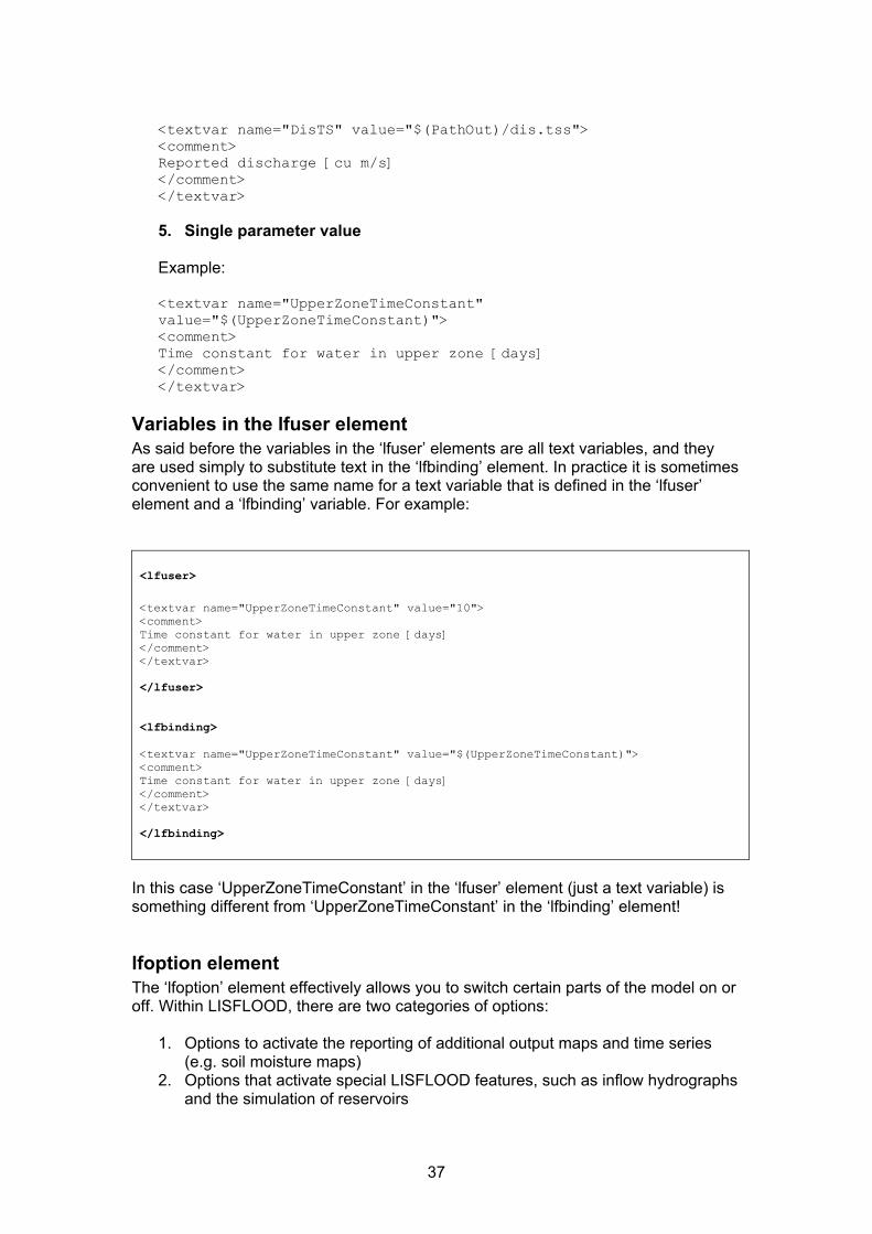
37

<textvar name="DisTS" value="$(PathOut)/dis.tss"> <comment> Reported discharge [cu m/s] </comment> </textvar> 5. Single parameter value Example:

<textvar name="UpperZoneTimeConstant" value="$(UpperZoneTimeConstant)"> <comment> Time constant for water in upper zone [days] </comment> </textvar>

Variables in the lfuser element As said before the variables in the ‘lfuser’ elements are all text variables, and they are used simply to substitute text in the ‘lfbinding’ element. In practice it is sometimes convenient to use the same name for a text variable that is defined in the ‘lfuser’ element and a ‘lfbinding’ variable. For example: <lfuser>

<textvar name="UpperZoneTimeConstant" value="10"> <comment> Time constant for water in upper zone [days] </comment> </textvar> </lfuser> <lfbinding> <textvar name="UpperZoneTimeConstant" value="$(UpperZoneTimeConstant)"> <comment> Time constant for water in upper zone [days] </comment> </textvar> </lfbinding>

In this case ‘UpperZoneTimeConstant’ in the ‘lfuser’ element (just a text variable) is something different from ‘UpperZoneTimeConstant’ in the ‘lfbinding’ element!

lfoption element The ‘lfoption’ element effectively allows you to switch certain parts of the model on or off. Within LISFLOOD, there are two categories of options:

1. Options to activate the reporting of additional output maps and time series (e.g. soil moisture maps)

2. Options that activate special LISFLOOD features, such as inflow hydrographs and the simulation of reservoirs

38

Viewing available options You can view all options by running LISFLOOD with the --listoptions flag. For each option, the following information is listed: OptionName Choices DefaultValue ‘OptionName’ -as you might have guessed already- simply is the name of the option. ‘Choices’ indicates the possible values of the option, and ‘DefaultValue’ describes the default behaviour. For instance, if you look at the reservoir option: simulateReservoirs choices=(1,0) default=0 you see that the value of this option is either 0 (off) or 1 (on), and that the default value is 0 (off, i.e. do not simulate any reservoirs). The information on the reporting options is a little bit different (and slightly confusing). Looking at the option for reporting discharge maps: repDischargeMaps choices=(1) noDefault By default, discharge maps are not reported, so you would expect something like “default=0”. However, due to the way options are defined internally in the model, in this case we have no default value, which means it is switched off.4 Report options that are switched on by default look like this: repStateMaps choices=(1) default=1 To minimise the confusion, you should:

1. Ignore the “Choices” item 2. Interpret “noDefault” as “default=0”

This is all a bit confusing, and the displaying of option information may well change in future LISFLOOD versions.

Defining options Within the ‘lfoptions’ element of the settings file, each option is defined using a ‘setoption’ element, which has the attributes ‘name’ and ‘choice’ (i.e. the actual value). For example: <lfoptions> <setoption choice="1" name="inflow" /> </lfoptions>

4 The reason why –listoptions produces “default=0” for the reservoirs option, is that –internally within the model- the reservoir option consists of two blocks of code: one block is the actual reservoir code, and another one is some dummy code that is activated if the reservoirs option is switched off (the dummy code is needed because some internal model variables that are associated with reservoirs need to be defined, even if no reservoirs are simulated). Both blocks are associated with “simulateReservoirs=1” and “simulateReservoirs=0”, respectively, where the “simulateReservoirs=0” block is marked as the default choice. In case of the “repDischargeMaps” option, there is no block of code that is associated with “repDischargeMaps=0”, hence formally there is no default value.

39

You are not obliged to use any options: if you leave the ‘lfoptions’ element empty, LISFLOOD will simply run using the default values (i.e. run model without optional modules; only report most basic output files). However, the ‘lfoptions’ element itself (i.e. <lfoptions> </lfoptions>) has to be present, even if empty!

40

41

6. Preparing the settings file This chapter describes how to prepare your own settings file. Instead of writing the settings file completely from scratch, we suggest to use the settings template that is provided with LISFLOOD as a starting point. In order to use the template, you should make sure the following requirements are met:

• All input maps and tables are named according to default file names (see Chapter 4)

• All base maps are in one directory • All tables are in one directory • All meteo input is in one directory • All Leaf Area Index input is in one directory • An (empty) directory where all model data can be written exists

If this is all true, the settings file can be prepared very quickly by editing the items in the ‘lfuser’ element. The following is a detailed description of the different sections of the ‘lfuser’ element. The present LISFLOOD version contains 24 process-related parameters (not taking into account the parameters that are defined through the base maps and lookup tables). These are all defined in the ‘lfuser’ element, and default values are given for each of them. Even though any of these parameters can be treated as calibration constants, doing so for all of them would lead to serious over-parameterisation problems. In the description of these parameters we will therefore provide some suggestions as to which parameters should be used for calibration, and which one are better left untouched.

Time-related constants The ‘lfuser’ section starts with a number of constants that are related to the simulation period and the time interval used. These are all defined as single values.

42

<comment> ************************************************************** TIME-RELATED CONSTANTS ************************************************************** </comment> <textvar name="DtSec" value="86400"> <comment> timestep [seconds] </comment> </textvar> <textvar name="DtSecChannel" value="86400"> <comment> Sub time step used for kinematic wave channel routing [seconds] Within the model,the smallest out of DtSecChannel and DtSec is used </comment> </textvar> <textvar name="StepStart" value="1"> <comment> Number of first time step in simulation </comment> </textvar> <textvar name="StepEnd" value="10"> <comment> Number of last time step in simulation </comment> </textvar> <textvar name="ReportSteps" value="endtime"> <comment> Time steps at which to write model state maps (i.e. only those maps that would be needed to define initial conditions for succeeding model run) </comment> </textvar>

DtSec is the simulation time interval in seconds. It has a value of 86400 for a daily time interval, 3600 for an hourly interval, etcetera DtSecChannel is the simulation time interval used by the kinematic wave channel routing (in seconds). Using a value that is smaller than DtSec may result in a better simulation of the overall shape the calculated hydrograph (at the expense of requiring more computing time) StepStart is the number of the first time step in your simulation. It is normally set to 1. Other (larger) values can be used if you want to run LISFLOOD for only a part of the time period for which you have meteo and LAI maps. StepEnd is the number of the last time step in your simulation. ReportSteps defines the time step number(s) at which the model state (i.e. all maps that you would need to define the initial conditions of a succeeding model run) is written. You can define this parameter as a (comma separated) list of time steps. For example:

<textvar name="ReportSteps" value="10,20,40">

will result in state maps being written at time steps 10, 20 and 40. For the last time step of a model run you can use the special ‘endtime’ keyword, e.g.:

<textvar name="ReportSteps" value="endtime">

43

Alternatively, in some cases you may need the state maps at regular intervals. In that case you can use the following syntax:

<textvar name="ReportSteps" value="start+increment..end">

For instance, in the following example state maps are written every 5th time step, starting at time step 10, until the last time step:

<textvar name="ReportSteps" value="10+5..endtime">

Parameters related to evapo(transpi)ration and interception The following parameters are all related to the simulation of evapo(transpi)ration and rainfall interception. Although they can all be defined as either a single value or as a map, we recommend using the single values that are included in the template. We do not recommend using any of these parameters as calibration constants. <comment> ************************************************************** PARAMETERS RELATED TO EVAPO(TRANSPI)RATION AND INTERCEPTION ************************************************************** </comment> <textvar name="CalEvaporation" value="1"> <comment> Multiplier applied to potential evapo(transpi)ration rates </comment> </textvar> <textvar name="LeafDrainageTimeConstant" value="1"> <comment> Time constant for water in interception store [days] </comment> </textvar> <textvar name="kdf" value="0.72"> <comment> Average extinction coefficient for the diffuse radiation flux varies with crop from 0.4 to 1.1 (Goudriaan (1977)) </comment> </textvar> <textvar name="AvWaterRateThreshold" value="5"> <comment> Critical amount of available water (expressed in [mm/day]!), above which 'Days Since Last Rain' parameter is set to 1 </comment> </textvar>

CalEvaporation is a multiplier that is applied to the potential evapo(transpi)ration input (ET0, EW0 and ES0) [-]

LeafDrainageTimeConstant (Tint in Eq 2-11) is the time constant for the interception store [days]

kdf is the average extinction for the diffuse radiation flux (Goudriaan, 1977). it is used to calculate the extinction coefficient for global radiation, κgb ,which is used in Equations 2-9, 2-14 and 2-19 [-] AvWaterRateThreshold defines a critical amount of water that is used as a threshold for resetting the variable Dslr in Eq 2-20. Because the equation was

44

originally developed for daily timesteps only, the threshold is currently defined (somewhat confusingly) as an equivalent intensity in [mm day-1]

Parameters related to snow and frost The following parameters are all related to the simulation of snow accumulation, snowmelt and frost. All these parameters can be defined as either single values or maps. We recommend to start out by leaving them all at their default values. If prior data suggest major under- or overcatch problems in the observed snowfall, SnowFactor can be adjusted accordingly. SnowMeltCoef may be used as a calibration constant, but since snow observations are typically associated with large uncertainty bands, the calibration may effectively just be compensating for these input errors.

45

<comment> ************************************************************** SNOW AND FROST RELATED PARAMETERS ************************************************************** </comment> <textvar name="SnowFactor" value="1"> <comment> Multiplier applied to precipitation that falls as snow </comment> </textvar> <textvar name="SnowMeltCoef" value="4.5"> <comment> Snowmelt coefficient [mm/deg C /day] See also Martinec et al., 1998. </comment> </textvar> <textvar name="TempMelt" value="0.0"> <comment> Average temperature at which snow melts </comment> </textvar> <textvar name="TempSnow" value="1.0"> <comment> Average temperature below which precipitation is snow </comment> </textvar> <textvar name="TemperatureLapseRate" value="0.0065"> <comment> Temperature lapse rate with altitude [deg C / m] </comment> </textvar> <textvar name="Afrost" value="0.97"> <comment> Daily decay coefficient, (Handbook of Hydrology, p. 7.28) </comment> </textvar> <textvar name="Kfrost" value="0.57"> <comment> Snow depth reduction coefficient, [cm-1], (HH, p. 7.28) </comment> </textvar> <textvar name="SnowWaterEquivalent" value="0.45"> <comment> Snow water equivalent, (based on snow density of 450 kg/m3) (e.g. Tarboton and Luce, 1996) </comment> </textvar> <textvar name="FrostIndexThreshold" value="56"> <comment> Degree Days Frost Threshold (stops infiltration, percolation and capillary rise) Molnau and Bissel found a value 56-85 for NW USA. </comment> </textvar>

SnowFactor is a multiplier that is applied to the rate of precipitation in case the precipitation falls as snow. Since snow is commonly underestimated in meteorological observation data, setting this multiplier to some value greater than 1 can counteract for this [-]

46

SnowMeltCoef (Cm in Eq 2-3) is the degree-day factor that controls the rate of snowmelt [mm °C-1 day-1] TempMelt (Tm in Eq 2-3) is the average temperature above which snow starts to melt [°C] TempSnow is the average temperature below which precipitation is assumed to be snow [°C] TemperatureLapseRate (L in Figure 2.2) is the temperature lapse rate that is used to estimate average temperature at the centroid of each pixel’s elevation zones [°C m-1] Afrost (A in Eq 2-4) is the frost index decay coefficient [day-1]. It has a value in the range 0-1. Kfrost (K in Eq 2-4) is a snow depth reduction coefficient [cm-1] SnowWaterEquivalent (wes in Eq 2-4) is the equivalent water depth of a given snow cover, expressed as a fraction [-] FrostIndexThreshold is the critical value of the frost index (Eq 2-5) above which the soil is considered frozen [°C day-1]

Infiltration parameters The following two parameters control the simulation of infiltration and preferential flow. Both are empirical parameters that are treated as calibration constants, and both can be defined as single values or maps. <comment> ************************************************************** INFILTRATION PARAMETERS ************************************************************** </comment> <textvar name="b_Xinanjiang" value="0.1"> <comment> Power in Xinanjiang distribution function </comment> </textvar> <textvar name="PowerPrefFlow" value="3"> <comment> Power that controls increase of proportion of preferential flow with increased soil moisture storage </comment> </textvar>

b_Xinanjiang (b in Eq 2-23) is the power in the infiltration equation [-] PowerPrefFlow (cpref in Eq 2-25) is the power in the preferential flow equation [-]

47

Groundwater parameters The following parameters control the simulation shallow and deeper groundwater. GwLossFraction should be kept at 0 unless prior information clearly indicates that groundwater is lost beyond the catchment boundaries (or to deep groundwater systems). The other parameters are treated as calibration constants. All these parameters can be defined as single values or maps. <comment> ************************************************************** GROUNDWATER RELATED PARAMETERS ************************************************************** </comment> <textvar name="UpperZoneTimeConstant" value="10"> <comment> Time constant for water in upper zone [days] </comment> </textvar> <textvar name="LowerZoneTimeConstant" value="1000"> <comment> Time constant for water in lower zone [days] This is the average time a water 'particle' remains in the reservoir if we had a stationary system (average inflow=average outflow) </comment> </textvar> <textvar name="GwPercValue" value="0.5"> <comment> Maximum rate of percolation going from the Upper to the Lower response box [mm/day] </comment> </textvar> <textvar name="GwLossFraction" value="0"> <comment> Maximum loss rate out of Lower response box, expressed as a fraction of lower zone outflow. Fraction [-], range 0-1 A value of 0 (closed lower boundary) is recommended as a starting value </comment> </textvar>

UpperZoneTimeConstant (Tuz in Eq 2-42) is the time constant for the upper groundwater zone [days] LowerZoneTimeConstant (Tlz in Eq 2-43) is the time constant for the lower groundwater zone [days] GwPercValue (GWperc in Eq 2-44) is the maximum rate of percolation going from the upper to the lower groundwater zone [mm day-1] GwLossFraction (floss in Eq 2-45) is the rate of flow out of the lower groundwater zone, expressed as a fraction [-] of the total outflow. Hence, the value of GwLossFraction is always between 0 and 1

Routing parameters These parameters are all related to the routing of water in the channels as well as the routing of surface runoff. The multiplier CalChanMan can be used to fine-tune the timing of the channel routing, and it may be defined as either a single value or a map. All other parameters should be kept at their default values.

48

<comment> ************************************************************** ROUTING PARAMETERS ************************************************************** </comment> <textvar name="CalChanMan" value="1"> <comment> Multiplier applied to Channel Manning's n </comment> </textvar> <textvar name="beta" value="0.6"> <comment> kinematic wave parameter: 0.6 is for broad sheet flow </comment> </textvar> <textvar name="OFDepRef" value="5"> <comment> Reference depth of overland flow [mm], used to compute overland flow Alpha for kin. wave </comment> </textvar> <textvar name="GradMin" value="0.001"> <comment> Minimum slope gradient (for kin. wave: slope cannot be 0) </comment> </textvar> <textvar name="ChanGradMin" value="0.0001"> <comment> Minimum channel gradient (for kin. wave: slope cannot be 0) </comment> </textvar>

CalChanMan is a multiplier that is applied to the Manning’s roughness maps of the channel system [-]

beta is routing coefficient βk in Equations 2-51, 2-52, 2-54 and 2-57 [-] OFDepRef is a reference flow depth from which the flow velocity of the surface runoff is calculated [mm] GradMin is a lower limit for the slope gradient used in the calculation of the surface runoff flow velocity [m m-1] ChanGradMin is a lower limit for the channel gradient used in the calculation of the channel flow velocity [m m-1]

Parameters related to numerics This category only contains one parameter at the moment, which can only be a single value. We strongly recommend keeping this parameter at its default value.

49

<comment> ************************************************************** PARAMETERS RELATED TO NUMERICS ************************************************************** </comment> <textvar name="CourantCrit" value="0.4"> <comment> Minimum value for Courant condition in soil moisture routine </comment> </textvar>

CourantCrit (Ccrit in Eq 2-36) is the critical Courant number which controls the numerical accuracy of the simulated soil moisture fluxes [-]. Any value between 0 and 1 can be used, but using values that are too high can lead to unrealistic “jumps” in the simulated soil moisture, whereas very low values result in reduced computational performance (because many iterations will be necessary to obtain the required accuracy). Values above 1 should never be used, as they will result in a loss of mass balance. In most cases the default value of 0.4 results in sufficiently realistic simulations using just a few iterations.

File paths Here you can specify where all the input files are located, and where output should be written. Note that you can use both forward and backward slashes on both Windows and Linux-based systems without any problem (when LISFLOOD reads the settings file it automatically formats these paths according to the conventions used by the operating system used). The default settings template contains relative paths, which in most cases allows you to run the model directly without changing these settings (assuming that you execute LISFLOOD from the root directory of your catchment).

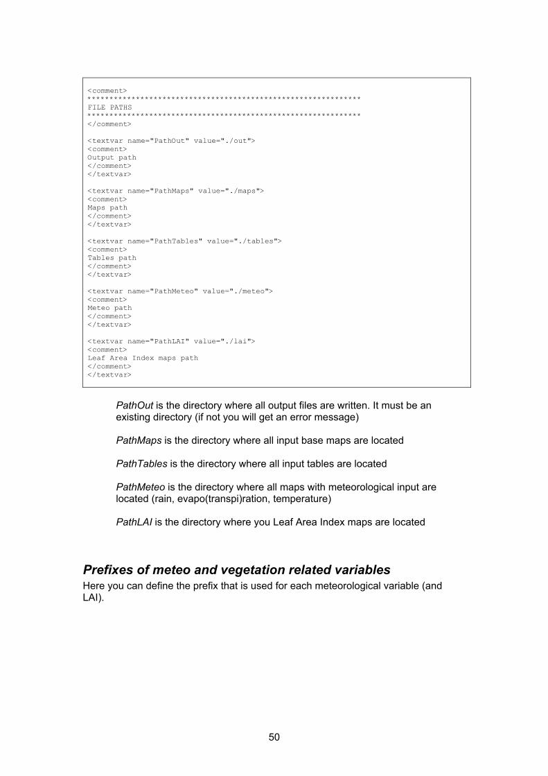
50

<comment> ************************************************************** FILE PATHS ************************************************************** </comment> <textvar name="PathOut" value="./out"> <comment> Output path </comment> </textvar> <textvar name="PathMaps" value="./maps"> <comment> Maps path </comment> </textvar> <textvar name="PathTables" value="./tables"> <comment> Tables path </comment> </textvar> <textvar name="PathMeteo" value="./meteo"> <comment> Meteo path </comment> </textvar> <textvar name="PathLAI" value="./lai"> <comment> Leaf Area Index maps path </comment> </textvar>

PathOut is the directory where all output files are written. It must be an existing directory (if not you will get an error message) PathMaps is the directory where all input base maps are located PathTables is the directory where all input tables are located PathMeteo is the directory where all maps with meteorological input are located (rain, evapo(transpi)ration, temperature) PathLAI is the directory where you Leaf Area Index maps are located

Prefixes of meteo and vegetation related variables Here you can define the prefix that is used for each meteorological variable (and LAI).

51

<comment> ************************************************************** PREFIXES OF METEO AND VEGETATION RELATED VARIABLES ************************************************************** </comment> <textvar name="PrefixPrecipitation" value="pr"> <comment> prefix precipitation maps </comment> </textvar> <textvar name="PrefixTavg" value="ta"> <comment> prefix average temperature maps </comment> </textvar> <textvar name="PrefixE0" value="e"> <comment> prefix E0 maps </comment> </textvar> <textvar name="PrefixES0" value="es"> <comment> prefix ES0 maps </comment> </textvar> <textvar name="PrefixET0" value="et"> <comment> prefix ET0 maps </comment> </textvar> <textvar name="PrefixLAI" value="lai"> <comment> prefix LAI maps </comment> </textvar>

Each variable is read as a stack of maps. The name of each map starts with prefix, and ends with the number of the time step. All characters in between are filled with zeroes. The name of each map is made up of a total of 11 characters: 8 characters, a dot and a 3-character suffix. For instance, using a prefix ‘pr’ we get: pr000000.007 : at time step 7 pr000035.260 : at time step 35260

To avoid unexpected behaviour, never use numbers in the prefix! For example: PrefixRain=pr10 For the first time step this yields the following file name: pr100000.001

But this is actually interpreted as time step 100,000,001! Therefore, do not use numbers in the prefix! The corresponding part of the settings file is pretty self-explanatory:

52

PrefixPrecipitation is the prefix of the precipitation maps PrefixTavg is the prefix of the daily average temperature maps PrefixE0 is the prefix of the potential open-water evaporation maps PrefixES0 is the prefix of the potential bare-soil evaporation maps PrefixET0 is the prefix of the potential (reference) evapotranspiration maps PrefixLAI is the prefix of the Leaf Area Index maps

Initial conditions As with the calibration parameters you can use both maps and single values to define the catchment conditions at the start of a simulation. Note that a couple of variables can be initialized internally in the model (explained below). Also, be aware that the initial conditions define the state of the model at t=(StepStart -1). As long as StepStart equals 1 this corresponds to t=0, but for larger values of StepStart this is (obviously) not the case! <group> <comment> ************************************************************** INITIAL CONDITIONS (maps or single values) ************************************************************** </comment> <textvar name="WaterDepthInitValue" value="0"> <comment> initial overland flow water depth [mm] </comment> </textvar> <textvar name="SnowCoverAInitValue" value="0"> <comment> initial snow depth in snow zone A [mm] </comment> </textvar> <textvar name="SnowCoverBInitValue" value="0"> <comment> initial snow depth in snow zone B [mm] </comment> </textvar> <textvar name="SnowCoverCInitValue" value="0"> <comment> initial snow depth in snow zone C [mm] </comment> </textvar> <textvar name="FrostIndexInitValue" value="0"> <comment> initial Frost Index value </comment> </textvar>

53

<textvar name="CumIntInitValue" value="0"> <comment> cumulative interception [mm] </comment> </textvar> <textvar name="UZInitValue" value="0"> <comment> water in upper store [mm] </comment> </textvar> <textvar name="DSLRInitValue" value="1"> <comment> days since last rainfall </comment> </textvar> </group> <group> <comment> ************************************************************** The following variables can also be initialized in the model internally. if you want this to happen set them to bogus value of -9999 ************************************************************** </comment> <textvar name="LZInitValue" value="-9999"> <comment> water in lower store [mm] -9999: use steady-state storage </comment> </textvar> <textvar name="TotalCrossSectionAreaInitValue" value="-9999"> <comment> initial cross-sectional area of flow in channel[m2] -9999: use half bankfull </comment> </textvar> <textvar name="ThetaInit1Value" value="-9999"> <comment> initial soil moisture content layer 1 -9999: use field capacity values </comment> </textvar> <textvar name="ThetaInit2Value" value="-9999"> <comment> initial soil moisture content layer 2 -9999: use field capacity values </comment> </textvar> <textvar name="LZAvInflowEstimate" value="1000"> <comment> Estimated average inflow [mm/day] into lower groundwater zone Used to calculated steady-state initial lower zone storage Use very high value (e.g. 1000) if you don't have any estimate (in that case steady-state storage bazed on GwPercValue, although this may give some initialisation problems) This parameter ONLY affects the simulation results if LZInitValue is set to -9999 !! Initialisation speedup parameter, not a calibration parameter! </comment> </textvar> </group>

54

WaterDepthInitValue is the initial amount of water on the soil surface [mm] SnowCoverInitAValue is the initial snow cover on the soil surface in elevation zone A [mm] SnowCoverInitBValue is the initial snow cover on the soil surface in elevation zone B [mm] SnowCoverInitCValue is the initial snow cover on the soil surface in elevation zone C [mm] FrostIndexInitValue (F in Eq 2-5) is the initial value of the frost index [°C day-

1] CumIntInitValue is the initial interception storage [mm] UZInitValue is the initial storage in the upper groundwater zone [mm] DSLRInitValue (Dslr in Eq 2-20) is the initial number of days since the last rainfall event [days] LZInitValue is the initial storage in the lower groundwater zone [mm]. In order to avoid initialization problems it is possible to let the model calculate a ‘steady state’ storage that will usually minimize any initialization problems. This feature is described in detail in Chapter 7 of this User Manual. To activate it, simply set LZInitValue to -9999. TotalCrossSectionAreaInitValue is the initial cross-sectional area [m2] of the water in the river channels (a substitute for initial discharge, which is directly dependent on this). A value of -9999 sets the initial amount of water in the channel to half bankfull. ThetaInit1Value is the initial moisture content [mm3 mm-3] of the upper soil layer. A value of -9999 will set the initial soil moisture content to field capacity. ThetaInit2Value is the initial moisture content [mm3 mm-3] of the lower soil layer. A value of -9999 will set the initial soil moisture content to field capacity LZAvInflowEstimate is an estimate of the average rate [mm day-1] at which water flows into the lower groundwater zone. This can be used to speed up the initialisation of the lower zone. LISFLOOD’s ‘repLZAvInflowMap’ option produces a map that can be used for optimized values of LZAvInflowEstimate at each pixel. For more details about this feature please have a look at Chapter 7 of this User Manual.

Running the model To run the model, start up a command prompt (Windows) or a console window (Linux) and type ‘lisflood’ followed by the name of the settings file, e.g.: lisflood settings.xml If everything goes well you should see something like this:

55

LISFLOOD version October 3 2007 Water balance and flood simulation model for large catchments (C) Institute for Environment and Sustainability Joint Research Centre of the European Commission TP261, I-21020 Ispra (Va), Italy Created: X:\test\txlGsbMlbr.tmp pcrcalc version: Oct 3 2007 (win32) Executing timestep 1

Using options As explained in Chapter 5, the ‘lfoptions’ element gives you additional control over what LISFLOOD is doing. Using options it is possible to switch certain parts of the model on or off. This way you can tell the model exactly which output files are reported and which ones aren’t. Also, they can be used to activate a number of additional model features, such as the simulation of reservoirs and inflow hydrographs. The table below lists all currently implemented options and their corresponding defaults. All currently implemented options are switches (1= on, 0=off). You can set as many options as you want (or none at all). Table 6.1 lists all currently implemented options5. Note that each option generally requires additional items in the settings file. For instance, using the inflow hydrograph option requires an input map and time series, which have to be specified in the settings file. If you want to report discharge maps at each time step, you will first have to specify under which name they will be written. The template settings file that is provided with LISFLOOD always contains file definitions for all optional output maps and time series. The use of the output options is described in detail in Chapter 8.

5 Actually, the –listoptions switch will show you a couple of options that are not listed in Table 6.1. These are either debugging options (which are irrelevant to the model user) or experimental features that may not be completely finalised (and thus remain undocumented here until they are)

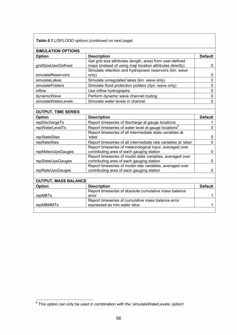
56

Table 6.1 LISFLOOD options (continued on next page)

SIMULATION OPTIONS Option Description Default

gridSizeUserDefined Get grid size attributes (length, area) from user-defined maps (instead of using map location attributes directly) 0

simulateReservoirs Simulate retention and hydropower reservoirs (kin. wave only) 0

simulateLakes Simulate unregulated lakes (kin. wave only) 0simulatePolders Simulate flood protection polders (dyn. wave only) 0inflow Use inflow hydrographs 0dynamicWave Perform dynamic wave channel routing 0simulateWaterLevels Simulate water levels in channel 0 OUTPUT, TIME SERIES Option Description DefaultrepDischargeTs Report timeseries of discharge at gauge locations 1repWaterLevelTs Report timeseries of water level at gauge locations6 0

repStateSites Report timeseries of all intermediate state variables at 'sites' 0

repRateSites Report timeseries of all intermediate rate variables at 'sites' 0

repMeteoUpsGauges Report timeseries of meteorological input, averaged over contributing area of each gauging station 0

repStateUpsGauges Report timeseries of model state variables, averaged over contributing area of each gauging station 0

repRateUpsGauges Report timeseries of model rate variables, averaged over contributing area of each gauging station 0

OUTPUT, MASS BALANCE Option Description Default

repMBTs Report timeseries of absolute cumulative mass balance error 1

repMBMMTs Report timeseries of cumulative mass balance error expressed as mm water slice 1

6 This option can only be used in combination with the ‘simulateWaterLevels’ option!

57

Table 6.1 LISFLOOD options (continued from previous page) OUTPUT, MAPS, DISCHARGE Option Description DefaultrepDischargeMaps Report maps of discharge (for each time step) 0repWaterLevelMaps7 Report maps of water level in channel (for each time step) 0 OUTPUT, MAPS, STATE VARIABLES (all, at selected time steps) Option Description Default

repStateMaps Report maps of model state variables (as defined by "ReportSteps" variable) 1

repEndMaps8 Report maps of model state variables (at last time step) 0 OUTPUT, MAPS, STATE VARIABLES Option Description DefaultrepDSLRMaps Report maps of days since last rain (for each time step) 0repFrostIndexMaps Report maps of frost index (for each time step) 0

repWaterDepthMaps Report maps of depth of water layer on soil surface (for each time step) 0

repSnowCoverMaps Report maps of snow cover (for each time step) 0repCumInterceptionMaps Report maps of interception storage (for each time step) 0repTheta1Maps Report maps of soil moisture layer 1(for each time step) 0repTheta2Maps Report maps of soil moisture layer 2 (for each time step) 0repUZMaps Report maps of upper zone storage (for each time step) 0repLZMaps Report maps of lower zone storage (for each time step) 0repChanCrossSection Maps

Report maps of channel cross-sectional area (for each time step) 0

OUTPUT, MAPS, METEOROLOGICAL FORCING VARIABLES Option Description DefaultrepPrecipitationMaps Report maps of precipitation (for each time step) 0repTavgMaps Report maps of average temperature (for each time step) 0

repETRefMaps Report maps of potential reference evapotranspiration (for each time step) 0

repESRefMaps Report maps of potential soil evaporation (for each time step) 0

repEWRefMaps Report maps of potential open water evaporation (for each time step) 0

7 This option can only be used in combination with the ‘simulateWaterLevels’ option! 8 Deprecated; this feature may not be supported in forthcoming LISFLOOD releases. Use repStateMaps instead, which gives you the same maps with the added possibility to report them for any required time step(s).

58

Table 6.1 LISFLOOD options (continued from previous page) OUTPUT, MAPS, RATE VARIABLES Option Description DefaultrepRainMaps Report maps of rain (excluding snow!) (for each time step) 0repSnowMaps Report maps of snow (for each time step) 0repSnowMeltMaps Report maps of snowmelt (for each time step) 0repInterceptionMaps Report maps of interception (for each time step) 0repLeafDrainageMaps Report maps of leaf drainage (for each time step) 0repTaMaps Report maps of actual transpiration (for each time step) 0repESActMaps Report maps of actual soil evaporation (for each time step) 0

repEWIntMaps Report maps of actual evaporation of intercepted water (for each time step) 0

repInfiltrationMaps Report maps of infiltration (for each time step) 0repPrefFlowMaps Report maps of preferential flow (for each time step) 0

repPercolationMaps Report maps of percolation from upper to lower soil layer (for each time step) 0

repSeepSubToGWMaps Report maps of seepage from lower soil layer to ground water (for each time step) 0

repGwPercUZLZMaps Report maps of percolation from upper to lower ground water zone (for each time step) 0

repGwLossMaps Report maps of loss from lower ground water zone (for each time step) 0

repSurfaceRunoffMaps Report maps of surface runoff (for each time step) 0repUZOutflowMaps Report maps of upper zone outflow (for each time step) 0repLZOutflowMaps Report maps of lower zone outflow (for each time step) 0

repTotalRunoffMaps Report maps of total runoff (surface + upper + lower zone) (for each time step) 0

OUTPUT, MAPS (MISCELLANEOUS) Option Description Default

repLZAvInflowMap Report computed average inflow rate into lower zone (map, at last time step) 0

repLZAvInflowSites Report computed average inflow rate into lower zone (time series, at points defined on sites map) 0

repLZAvInflowUpsGauges

Report computed average inflow rate into lower zone (time series, averaged over upstream area of each gauge location) 0

59

7. Initialisation of LISFLOOD

Introduction Just as any other hydrological model, LISFLOOD needs to have some estimate of the initial state (i.e. amount of water stored) of its internal state variables. Two situations can occur:

1. The initial state of all state variables is known (for example, the “end maps” of a daily water balance run are used to define the initial conditions of an hourly flood-event run)

2. The initial state of all state variables is unknown The second situation is the most common one, and this chapter presents an in-depth look at the initialisation of LISFLOOD. First the effect of the model’s initial state on the results of a simulation is demonstrated using a simple example. Then, LISFLOOD’s various initialisation options are discussed. Most of this chspter focuses on the initialisation of the lower groundwater zone, as this is the model storage component that is the most difficult to in initialise.

An example To better understand the impact of the initial model state on simulation results, let’s start with a simple example. Figure 7.1 shows 3 LISFLOOD simulations of soil moisture for the upper soil layer. In the first simulation, it was assumed that the soil is initially completely saturated. In the second one, the soil was assumed to be completely dry (i.e. at residual moisture content). Finally, a third simulation was done where the initial soil moisture content was assumed to be in between these two extremes.

Figure 7.1 Simulation of soil moisture in upper soil layer for a soil that is initially at saturation (s), at residual moisture content (r) and in between ([s+r]/2)

60

What is clear from the Figure is that the initial amount of moisture in the soil only has a marked effect on the start of each simulation; after a couple of months the three curves converge. In other words, the “memory” of the upper soil layer only goes back a couple of months (or, more precisely, for time lags of more than about 8 months the autocorrelation in time is negligible). In theory, this behaviour provides a convenient and simple way to initialise a model such as LISFLOOD. Suppose we want to do a simulation of the year 1995. We obviously don’t know the state of the soil at the beginning of that year. However, we can get around this by starting the simulation a bit earlier than 1995, say one year. In that case we use the year 1994 as a warm-up period, assuming that by the start of 1995 the influence of the initial conditions (i.e. 1-1-1994) is negligible. The very same technique can be applied to initialise LISFLOOD’s other state variables, such as the amounts of water in the lower soil layer, the upper groundwater zone, the lower groundwater zone, and in the channel.

Setting up a LISFLOOD run with warm-up period When setting up a model run that includes a warm-up period, most of the internal state variables can be simply set to 0 at the start of the run. This applies to the initial amount of water on the soil surface (WaterDepthInitValue), snow cover (SnowCoverInitValue), frost index (FrostIndexInitValue), interception storage (CumIntInitValue), and storage in the upper groundwater zone (UZInitValue). The initial value of the ‘days since last rainfall event’ (DSLRInitValue) is typically set to 1. For the remaining state variables, initialisation is somewhat less straightforward. The amount of water in the channel (defined by TotalCrossSectionAreaInitValue) is highly spatially variable (and limited by the channel geometry). The amount of water that can be stored in the upper and lower soil layers (ThetaInit1Value, ThetaInit2Value) is limited by the soil’s porosity. The lower groundwater zone poses special problems because of its overall slow response (discussed in a separate section below). Because of this, LISFLOOD provides the possibility to initialise these variables internally, and these special initialisation methods can be activated by setting the initial values of each of these variables to a special ‘bogus’ value of -9999. Table 7.1 summarises these special initialisation methods: Table 7.1 LISFLOOD special initialisation methods* Variable Description Initialisation method ThetaInit1Value initial soil moisture content

upper soil layer (V/V) set to soil moisture content at field capacity

ThetaInit2Value initial soil moisture content lower soil layer (V/V)

set to soil moisture content at field capacity

LZInitValue initial water in lower groundwater zone (mm)

set to steady-state storage

TotalCrossSectionAreaInitValue initial cross-sectional area of water in channels

set to half of bankfull depth

*) These special initialisation methods are activated by setting the value of each respective variable to a ‘bogus’ value of “-9999”

Note that the “-9999” ‘bogus’ value can only be used with the variables in Table 7.1; for all other variables they will produce nonsense results! The initialisation of the lower groundwater zone will be discussed in the next sections.

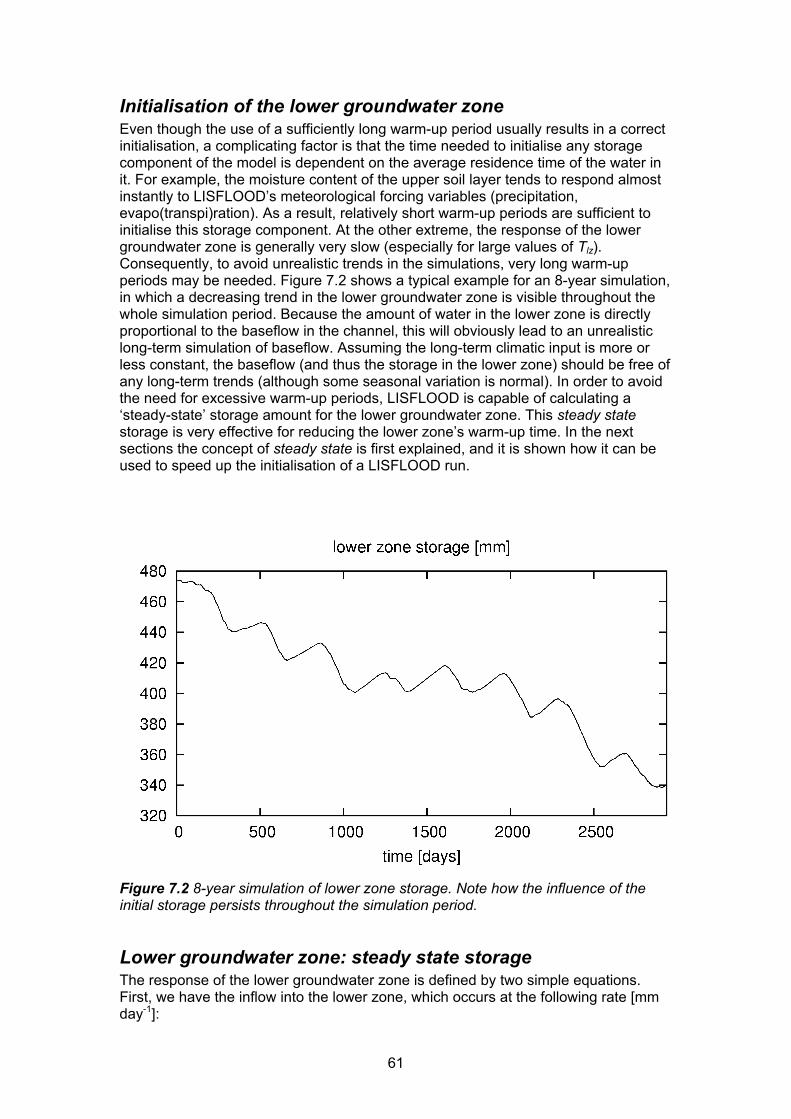
61

Initialisation of the lower groundwater zone Even though the use of a sufficiently long warm-up period usually results in a correct initialisation, a complicating factor is that the time needed to initialise any storage component of the model is dependent on the average residence time of the water in it. For example, the moisture content of the upper soil layer tends to respond almost instantly to LISFLOOD’s meteorological forcing variables (precipitation, evapo(transpi)ration). As a result, relatively short warm-up periods are sufficient to initialise this storage component. At the other extreme, the response of the lower groundwater zone is generally very slow (especially for large values of Tlz). Consequently, to avoid unrealistic trends in the simulations, very long warm-up periods may be needed. Figure 7.2 shows a typical example for an 8-year simulation, in which a decreasing trend in the lower groundwater zone is visible throughout the whole simulation period. Because the amount of water in the lower zone is directly proportional to the baseflow in the channel, this will obviously lead to an unrealistic long-term simulation of baseflow. Assuming the long-term climatic input is more or less constant, the baseflow (and thus the storage in the lower zone) should be free of any long-term trends (although some seasonal variation is normal). In order to avoid the need for excessive warm-up periods, LISFLOOD is capable of calculating a ‘steady-state’ storage amount for the lower groundwater zone. This steady state storage is very effective for reducing the lower zone’s warm-up time. In the next sections the concept of steady state is first explained, and it is shown how it can be used to speed up the initialisation of a LISFLOOD run.

Figure 7.2 8-year simulation of lower zone storage. Note how the influence of the initial storage persists throughout the simulation period.

Lower groundwater zone: steady state storage The response of the lower groundwater zone is defined by two simple equations. First, we have the inflow into the lower zone, which occurs at the following rate [mm day-1]:

62

)/,min(, tUZGWD perclzuz Δ= (7-1)

Here, GWperc [mm day-1] is a user-defined value (calibration constant), and UZ is the amount of water available in the upper groundwater zone [mm]. The rate of flow out of the lower zone [mm day-1] equals:

LZQlz ⋅=lzT

1 (7-2)

where Tlz is a reservoir constant [days], and LZ is the amount of water that is stored in the lower zone [mm]. Now, let’s do a simple numerical experiment: assuming that Duz,lz is a constant value, we can take some arbitrary initial value for LZ and then simulate (e.g. in a spreadsheet) the development over LZ over time. Figure 7.3 shows the results of 2 such experiments. In the upper Figure, we start with a very high initial storage (1500 mm). The inflow rate is fairly small (0.2 mm/day), and Tlz is quite small as well (which means a relatively short residence time of the water in the lower zone). What is interesting here is that, over time, the storage evolves asymptotically towards a constant state. In the lower Figure, we start with a much smaller initial storage (50 mm), but the inflow rate is much higher here (1.5 mm/day) and so is Tlz (1000 days). Here we see an upward trend, again towards a constant value. However, in this case the constant ‘end’ value is not reached within the simulation period, which is mainly because Tlz is set to a value for which the response is very slow. At this point it should be clear that what you see in these graphs is exactly the same behaviour that is also apparent in the ‘real’ LISFLOOD simulation in Figure 7.2. Being able to know the ‘end’ storages in Figure 7.3 in advance would be very helpful, because it would eliminate any trends. As it happens, this can be done very easily from the model equations. A storage that is constant over time means that the in- and outflow terms balance each other out. This is known as a steady state situation, and the constant ‘end’ storage is in fact the steady state storage. The rate of change of the lower zone’s storage at any moment is given by the continuity equation:

)()( tOtIdtdLZ

−= (7-3)

where I is the (time dependent) inflow (i.e. groundwater recharge) and O is the outflow rate. For a situation where the storage remains constant, we can write:

0)()(0 =−⇔= tOtIdtdLZ

(7-4)

63

Figure 7.3 Two 10-year simulations of lower zone storage with constant inflow. Upper Figure: high initial storage, storage approaches steady-state storage (dashed) after about 1500 days. Lower Figure: low initial storage, storage doesn’t reach steady-state within 10 years. This equation can be re-written as:

0T1)(lz

=⋅− LZtI (7-5)

Solving this for LZ gives the steady state storage:

64

)(Tlz tILZss ⋅= (7-6)

We can check this for our numerical examples: Tlz I LZss 250 0.2 50 1000 1.5 1500

which corresponds exactly to the results of Figure 7.3.

Steady-state storage in practice An actual LISFLOOD simulation differs from the previous example in 2 ways. First, in any real simulation the inflow into the lower zone is not constant, but varies in time. This is not really a problem, since LZss can be computed from the average recharge. However, this is something we do not know until the end of the simulation! Also, the inflow into the lower zone is controlled by the availability of water in the upper zone, which, in turn, depends on the supply of water from the soil. Hence, it is influenced by any calibration parameters that control behaviour of soil- and subsoil (e.g. Tuz, GWperc, b, and so on). This means that –when calibrating the model- the average recharge will be different for every parameter set. Note, however, that it will always be smaller than the value of GWperc, which is used as an upper limit in the model. There are now 2 different ways to proceed. Note that both procedures include a sufficiently long warm-up period! In general, using a warm-up period of 1 year is good enough.

Procedure 1: prior estimate of average recharge This is the most straightforward way to initialise the lower zone, and also the riskiest one:

1. Select LISFLOOD parameter set (in calibration) 2. Set ThetaInit1Value,ThetaInit2Value,LZInitValue and

TotalCrossSectionAreaInitValue to -9999 3. Make an estimate of the average recharge (i.e. the average flow of water

from the upper to the lower groundwater zone, expressed in [mm day-1]). Then set initialisation parameter LZAvInflowEstimate to this value. Remember that the actual recharge can never exceed the value of model parameter GWperc, and LISFLOOD will always base its steady-state storage estimate on the smallest value out of LZAvInflowEstimate and GWperc.9

4. Run the model What happens now is that LISFLOOD computes the initial state of LZ, assuming that the average recharge can be approximated by LZAvInflowEstimate. In general, initialising LISFLOOD like this is quite risky, and the simulated development of the lower zone will often still show (strong) long-term trends.

9 If you want to base your steady-state storage estimate on the assumption of an average recharge that equals the value of GWperc, you can do this by simply setting LZAvInflowEstimate to any ridiculously large value (e.g. 1000).

65

Procedure 2: use pre-run to calculate average recharge Here, we first do a “pre-run” that is used to calculate the average inflow into the lower zone. This average inflow can be reported as a map, which is then used in the actual run. This involves the following steps:

1. Set ThetaInit1Value,ThetaInit2Value,LZInitValue and TotalCrossSectionAreaInitValue to -9999

2. Activate the “repLZAvInflowMap” option by adding the following line to the ‘lfoptions’ element in the settings file:

<setoption name="repLZAvInflowMap" choice="1"></setoption>

3. Run the model 4. Find the map ‘lzavin.map’ in the output directory and copy it to another

location 5. Go back to the LISFLOOD settings file, and enter the name of ‘lzavin.map’

(including full path) for initialisation parameter LZAvInflowEstimate. For example:

<textvar name="LZAvInflowEstimate" value="D:\meuse\lzavin.map">

6. Switch off the “repLZAvInflowMap” option (optional, leaving it on will not do any harm, but it makes LISFLOOD run somewhat slower)

7. Run the model again using the modified settings file In this case, the initial state of LZ is computed for the correct average inflow, and the simulated storage in the lower zone throughout the simulation will not show any systematic (long-term) trends. The obvious price to pay for this is that the pre-run doubles the computational load. However, as long as the simulation period for the actual run and the pre-run are identical, the procedure gives a 100% guarantee that the development of the lower zone storage will be free of any systematic bias. Since the computed recharge values are dependent on the model parameterisation used, in a calibration setting the whole procedure must be repeated for each parameter set!

Checking the lower zone initialisation The presence of any initialisation problems of the lower zone can be checked by adding the following line to the ‘lfoptions’ element of the settings file:

<setoption name=" repStateUpsGauges" choice="1"></setoption> This tells the model to write the values of all state variables (averages, upstream of contributing area to each gauge) to time series files. The default name of the lower zone time series is ‘lzUps.tss’. Figure 7.4 shows an example of an 8-year simulation that was done both without (dashed line) and with a pre-run. The simulation without the pre-run shows a steady decreasing trend throughout the 8-year period, whereas the simulation for which the pre-run was used doesn’t show this long-term trend (although in this specific case a modest increasing trend is visible throughout the first 6 years of the simulation, but this is related to trends in the meteorological input).

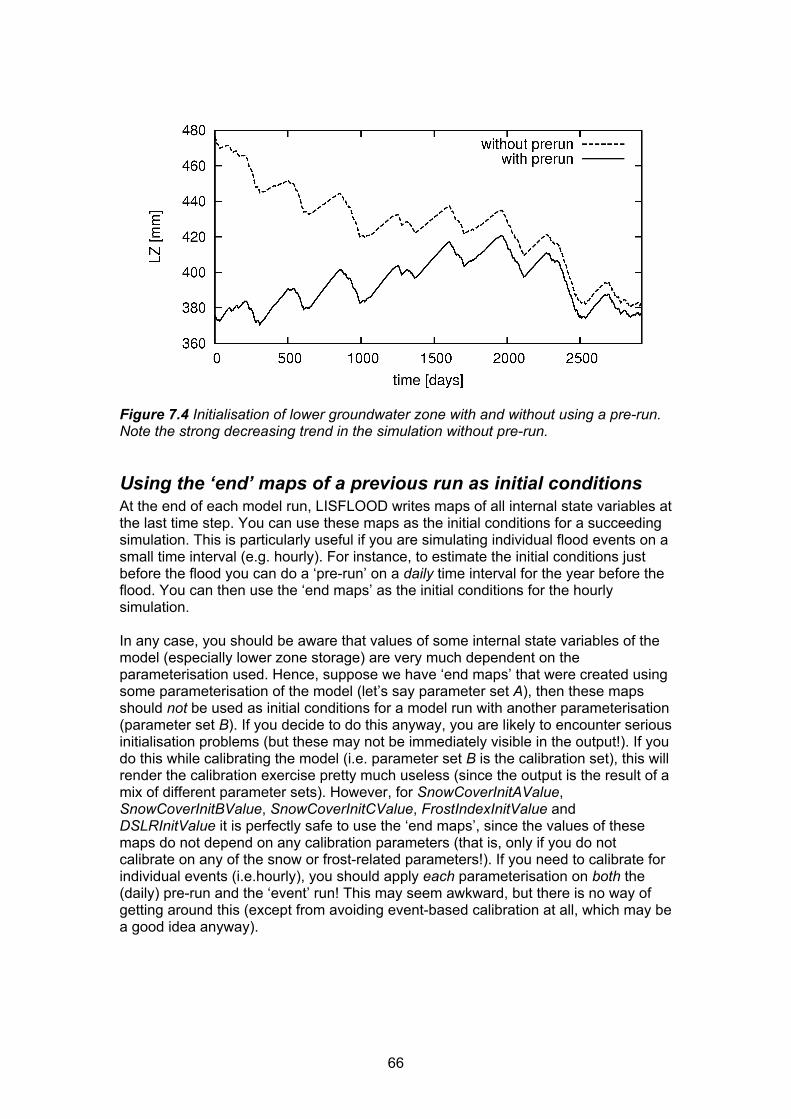
66

Figure 7.4 Initialisation of lower groundwater zone with and without using a pre-run. Note the strong decreasing trend in the simulation without pre-run.

Using the ‘end’ maps of a previous run as initial conditions At the end of each model run, LISFLOOD writes maps of all internal state variables at the last time step. You can use these maps as the initial conditions for a succeeding simulation. This is particularly useful if you are simulating individual flood events on a small time interval (e.g. hourly). For instance, to estimate the initial conditions just before the flood you can do a ‘pre-run’ on a daily time interval for the year before the flood. You can then use the ‘end maps’ as the initial conditions for the hourly simulation. In any case, you should be aware that values of some internal state variables of the model (especially lower zone storage) are very much dependent on the parameterisation used. Hence, suppose we have ‘end maps’ that were created using some parameterisation of the model (let’s say parameter set A), then these maps should not be used as initial conditions for a model run with another parameterisation (parameter set B). If you decide to do this anyway, you are likely to encounter serious initialisation problems (but these may not be immediately visible in the output!). If you do this while calibrating the model (i.e. parameter set B is the calibration set), this will render the calibration exercise pretty much useless (since the output is the result of a mix of different parameter sets). However, for SnowCoverInitAValue, SnowCoverInitBValue, SnowCoverInitCValue, FrostIndexInitValue and DSLRInitValue it is perfectly safe to use the ‘end maps’, since the values of these maps do not depend on any calibration parameters (that is, only if you do not calibrate on any of the snow or frost-related parameters!). If you need to calibrate for individual events (i.e.hourly), you should apply each parameterisation on both the (daily) pre-run and the ‘event’ run! This may seem awkward, but there is no way of getting around this (except from avoiding event-based calibration at all, which may be a good idea anyway).

67

Summary of LISFLOOD initialisation procedure From the foregoing it is clear that the initialisation of LISFLOOD can be done in a number of ways. Figure 7.5 gives an overview. As already stated in the introduction section, any LISFLOOD simulation will fall into either of the following two categories:

1. The initial state of all state variables is known and defined by the end state of a previous run. In this case you can use the ‘end’ maps of the previous run’s state variables as the initial conditions of you current run. Note that this requires that both simulations are run using exactly the same parameter set! Mixing parameter sets here will introduce unwanted artefacts into your simulation results.

2. The initial state of all state variables is unknown. In this case you should run the model with a sufficient warm-up period (one year will usually do), using the available special initialisation methods to initialise soil moisture, lower zone storage and the amount of water in the channel. In addition, you should first do a “pre-run” to calculate the average recharge into the lower zone. The average recharge map that is generated from the pre-run can subsequently be used as the average lower zone inflow estimate (LZAvInflowEstimate) in the actual simulation, which will avoid any initialisation problems of the lower groundwater zone.

Figure 7.5 LISFLOOD initialisation flowchart

68

69

8. Output generated by LISFLOOD

Default LISFLOOD output LISFLOOD can generate a wide variety of output. Output is generated as either maps (PCRaster format, which can be visualised with PCRaster’s ‘display’ application) or time series (can be visualised with PCRaster’s ‘timeplot’ application or any other plotting software that can read or import ASCII files). Reporting of output files can be switched on and off using options in the LISFLOOD settings file. Also, a number of output files are specific to other optional modules, such as the simulation of reservoirs. The following table lists all the output time series that are reported by default (note that the file names can always be changed by the user, although this is not recommended):

Table 8.1 LISFLOOD default output time series RATE VARIABLES AT GAUGES Description Units File name channel discharge m3/s dis.tss NUMERICAL CHECKS Description Units File name cumulative mass balance error m3 mbError.tss cumulative mass balance error, expressed as mm water slice (average over catchment)

mm mbErrorMm.tss

number of sub-steps needed for gravity-based soil moisture routine

- steps.tss

In addition to these time series, by default LISFLOOD reports maps of all state variables at the last timestep of a simulation. These maps can be used to define the initial conditions of a succeeding simulation. For instance, you can do a 1-year simulation on a daily time step, and use the ‘end maps’ of this simulation to simulate a flood event using an hourly time step. Table 8.2 lists all these maps. Note that some state variables are valid for the whole pixel, whereas others are only valid for a sub-domain of each pixel. This is indicated in the last column of the table.

70

Table 8.2 LISFLOOD default state variable output maps. These maps can be used to define the initial conditions of another simulation

DEFAULT OUTPUT MAPS LISFLOOD (option repStateMaps) Description Units File name10 Domain waterdepth at last time step mm wdepth00.xxx whole pixel channel cross-sectional area at last time step m2 chcross0.xxx channel days since last rain variable at last time step days dslr0000.xxx whole pixel snow cover zone A at last time step mm scova000.xxx snow zone A (1/3rd pixel)snow cover zone B at last time step mm scovb000.xxx snow zone B (1/3rd pixel)snow cover zone C at last time step mm scovc000.xxx snow zone C (1/3rd pixel)frost index at last time step degree-days frost000.xxx whole pixel cumulative interception at last time step mm cumint00.xxx whole pixel soil moisture upper layer at last time step mm3/mm3 thtop000.xxx permeable fraction pixelsoil moisture lower layer at last time step mm3/mm3 thsub000.xxx permeable fraction pixelwater in lower zone at last time step mm lz000000.xxx permeable fraction pixelwater in upper zone at last time step mm uz000000.xxx permeable fraction pixel

Additional output Apart from the default output, the model can –optionally- generate some additional time series and maps. Roughly this additional output falls in either of the following categories:

1. Time series with values of model state variables at user-defined locations (sites); reporting of these time series can be activated using the option repStateSites=1. Note that ‘sites’ can be either individual pixels or larger areas (e.g. catchments, administrative areas, and so on). In case of larger areas the model reports the average value for each respective area.

2. Time series with values of model rate variables at user-defined locations (sites); reporting of these time series can be activated using the option repRateSites=1

3. Time series with values of meteorological input variables, averaged over the area upstream of each gauge location; reporting of these time series can be activated using the option repMeteoUpsGauges=1

4. Time series with values of model state variables, averaged over area upstream of each gauge location; reporting of these time series can be activated using the option repStateUpsGauges=1

5. Time series with values of model rate variables, averaged over area upstream of each gauge location; reporting of these time series can be activated using the option repRateUpsGauges=1

6. Maps of discharge at each time step; reporting of these maps can be activated using the option repDischargeMaps=1

7. Maps with values of driving meteorological values at each time step 8. Maps with values of model rate variables at each time step 9. Maps or time series that are specific to other options (e.g. simulation of

reservoirs).

10 xxx represents the number of the last time step; e.g. or a 730-step simulation the end map of ‘waterdepth’ will be ‘wdepth00.730’, and so on.

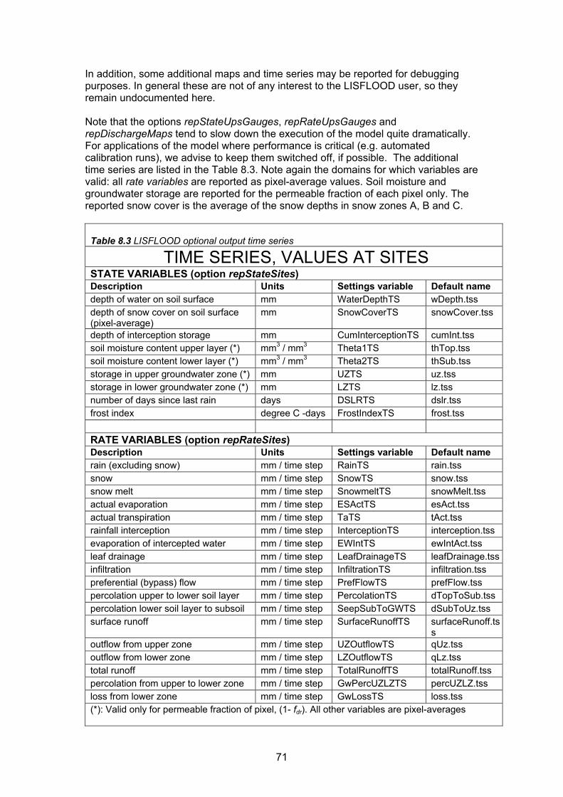
71

In addition, some additional maps and time series may be reported for debugging purposes. In general these are not of any interest to the LISFLOOD user, so they remain undocumented here. Note that the options repStateUpsGauges, repRateUpsGauges and repDischargeMaps tend to slow down the execution of the model quite dramatically. For applications of the model where performance is critical (e.g. automated calibration runs), we advise to keep them switched off, if possible. The additional time series are listed in the Table 8.3. Note again the domains for which variables are valid: all rate variables are reported as pixel-average values. Soil moisture and groundwater storage are reported for the permeable fraction of each pixel only. The reported snow cover is the average of the snow depths in snow zones A, B and C. Table 8.3 LISFLOOD optional output time series

TIME SERIES, VALUES AT SITES STATE VARIABLES (option repStateSites) Description Units Settings variable Default name depth of water on soil surface mm WaterDepthTS wDepth.tss depth of snow cover on soil surface (pixel-average)

mm SnowCoverTS snowCover.tss

depth of interception storage mm CumInterceptionTS cumInt.tss soil moisture content upper layer (*) mm3 / mm3 Theta1TS thTop.tss soil moisture content lower layer (*) mm3 / mm3 Theta2TS thSub.tss storage in upper groundwater zone (*) mm UZTS uz.tss storage in lower groundwater zone (*) mm LZTS lz.tss number of days since last rain days DSLRTS dslr.tss frost index degree C -days FrostIndexTS frost.tss RATE VARIABLES (option repRateSites) Description Units Settings variable Default name rain (excluding snow) mm / time step RainTS rain.tss snow mm / time step SnowTS snow.tss snow melt mm / time step SnowmeltTS snowMelt.tss actual evaporation mm / time step ESActTS esAct.tss actual transpiration mm / time step TaTS tAct.tss rainfall interception mm / time step InterceptionTS interception.tss evaporation of intercepted water mm / time step EWIntTS ewIntAct.tss leaf drainage mm / time step LeafDrainageTS leafDrainage.tssinfiltration mm / time step InfiltrationTS infiltration.tss preferential (bypass) flow mm / time step PrefFlowTS prefFlow.tss percolation upper to lower soil layer mm / time step PercolationTS dTopToSub.tss percolation lower soil layer to subsoil mm / time step SeepSubToGWTS dSubToUz.tss surface runoff mm / time step SurfaceRunoffTS surfaceRunoff.ts

s outflow from upper zone mm / time step UZOutflowTS qUz.tss outflow from lower zone mm / time step LZOutflowTS qLz.tss total runoff mm / time step TotalRunoffTS totalRunoff.tss percolation from upper to lower zone mm / time step GwPercUZLZTS percUZLZ.tss loss from lower zone mm / time step GwLossTS loss.tss (*): Valid only for permeable fraction of pixel, (1- fdr). All other variables are pixel-averages

72

Table 8.3 LISFLOOD optional output time series (continued)

TIME SERIES, AVERAGE UPSTREAM OF GAUGES METEOROLOGICAL INPUT VARIABLES (option repMeteoUpsGauges) Description Units Settings variable Default name precipitation mm/time step PrecipitationAvUpsTS precipUps.tss potential reference evapotranspiration

mm/time step ETRefAvUpsTS etUps.tss

potential evaporation from soil mm/time step ESRefAvUpsTS esUps.tss potential open water evaporation mm/time step EWRefAvUpsTS ewUps.tss average daily temperature °C TavgAvUpsTS tAvgUps.tss STATE VARIABLES (option repStateUpsGauges) Description Units Settings variable Default name depth of water on soil surface mm WaterDepthAvUpsTS wdepthUps.tss depth of snow cover on mm SnowCoverAvUpsTS snowCoverUps.tss depth of interception storage mm CumInterceptionAvUpsTS cumInterceptionUps.tss soil moisture upper layer (*) mm3 / mm3 Theta1AvUpsTS thTopUps.tss soil moisture lower layer (*) mm3 / mm3 Theta2AvUpsTS thSubUps.tss groundwater upper zone (*) mm UZAvUpsTS uzUps.tss groundwater lower zone (*) mm LZAvUpsTS lzUps.tss number of days since last rain days DSLRAvUpsTS dslrUps.tss frost index °C days-1 FrostIndexAvUpsTS frostUps.tss RATE VARIABLES (option repRateUpsGauges) Description Units Settings variable Default name rain (excluding snow) mm / time step RainAvUpsTS rainUps.tss snow mm / time step SnowAvUpsTS snowUps.tss snow melt mm / time step SnowmeltAvUpsTS snowMeltUps.tss actual evaporation mm / time step ESActAvUpsTS esActUps.tss actual transpiration mm / time step TaAvUpsTS tActUps.tss rainfall interception mm / time step InterceptionAvUpsTS interceptionUps.tss evaporation of intercepted water mm / time step EWIntAvUpsTS ewIntActUps.tss leaf drainage mm / time step LeafDrainageAvUpsTS leafDrainageUps.tss infiltration mm / time step InfiltrationAvUpsTS infiltrationUps.tss preferential (bypass) flow mm / time step PrefFlowAvUpsTS prefFlowUps.tss percolation upper to lower soil layer

mm / time step PercolationAvUpsTS dTopToSubUps.tss

percolation lower soil layer to subsoil

mm / time step SeepSubToGWAvUpsTS dSubToUzUps.tss

surface runoff mm / time step SurfaceRunoffAvUpsTS surfaceRunoffUps.tss outflow from upper zone mm / time step UZOutflowAvUpsTS qUzUps.tss outflow from lower zone mm / time step LZOutflowAvUpsTS qLzUps.tss total runoff mm / time step TotalRunoffAvUpsTS totalRunoffUps.tss percolation upper to lower zone mm / time step GwPercUZLZAvUpsTS percUZLZUps.tss loss from lower zone mm / time step GwLossTS lossUps.tss (*): Valid only for permeable fraction of pixel, (1- fdr). All other variables are pixel-averages

73

Table 8.3 LISFLOOD optional output time series (continued) WATER LEVEL IN CHANNEL (option repWaterLevelTs) Description Units Settings variable Default name water level in channel m (above

channel bottom)

WaterLevelTS waterLevel.tss

By default, the names of the reported discharge maps start with the prefix ‘dis’ and end with the time step number (the naming conventions are identical to the ones used for the input maps with meteorological variables, which is explained in Chapter 4). Table 8.4 summarises all options to report additional output maps. The previous remarks related to the domains foe which the state variable values are valid also apply to the maps listed in Table 8.4.

74

Table 8.4 LISFLOOD optional series of output maps (all units identical to the ones listed in Table 8.3) DISCHARGE Description Option Settings variable Prefix discharge repDischargeMaps DischargeMaps dis water level repWaterLevelMaps WaterLevelMaps wl METEOROLOGICAL INPUT VARIABLES Description Option Settings variable Prefix precipitation repPrecipitationMaps PrecipitationMaps pr potential reference evapotranspiration repETRefMaps ETRefMaps et potential evaporation from soil repESRefMaps ESRefMaps es potential open water evaporation repEWRefMaps EWRefMaps ew average daily temperature repTavgMaps TavgMaps tav STATE VARIABLES Description Option Settings variable Prefix depth of water on soil surface repWaterDepthMaps WaterDepthMaps wdep depth of snow cover on soil surface repSnowCoverMaps SnowCoverMaps scov depth of interception storage repCumInterceptionMaps CumInterceptionMaps cumint soil moisture content upper layer (*) repTheta1Maps Theta1Maps thtop soil moisture content lower layer (*) repTheta2Maps Theta2Maps thsub storage in upper groundwater zone (*) repUZMaps UZMaps uz storage in lower groundwater zone (*) repLZMaps LZMaps lz number of days since last rain repDSLRMaps DSLRMaps dslr frost index repFrostIndexMaps FrostIndexMaps frost RATE VARIABLES Description Option Settings variable Prefix rain (excluding snow) repRainMaps RainMaps rain snow repSnowMaps SnowMaps snow snow melt repSnowMeltMaps SnowMeltMaps smelt actual evaporation repESActMaps ESActMaps esact actual transpiration repTaMaps TaMaps tact rainfall interception repInterceptionMaps InterceptionMaps int evaporation of intercepted water repEWIntMaps EWIntMaps ewint leaf drainage repLeafDrainageMaps LeafDrainageMaps ldra infiltration repInfiltrationMaps InfiltrationMaps inf preferential (bypass) flow repPrefFlowMaps PrefFlowMaps pflow percolation upper to lower soil layer repPercolationMaps PercolationMaps to2su percolation lower soil layer to subsoil repSeepSubToGWMaps SeepSubToGWMaps su2gw surface runoff repSurfaceRunoffMaps SurfaceRunoffMaps srun outflow from upper zone repUZOutflowMaps UZOutflowMaps quz outflow from lower zone repLZOutflowMaps LZOutflowMaps qlz total runoff repTotalRunoffMaps TotalRunoffMaps trun percolation upper to lower zone repGwPercUZLZMaps GwPercUZLZMaps uz2lz loss from lower zone rep GwLossMaps GwLossMaps loss (*): Valid only for permeable fraction of pixel, (1- fdr). All other variables are pixel-averages

75

Finally, some additional output options exist that don’t fit in any of the above categories. They are listed in Table 8.5:

Table 8.5 LISFLOOD miscellaneous optional output OUTPUT RELATED TO LOWER ZONE INITIALISATION Description Option Settings variable Default nameaverage inflow into lower zone [mm day-1] repLZAvInflowMap LZAvInflowMap lzavin.map average inflow into lower zone [mm day-1] repLZAvInflowSites LZAvInflowTS lzAvIn.tss average inflow into lower zone [mm day-1] repLZAvInflowUpsGauges LZAvInflowAvUpsTS lzAvInUps.tss

76

77

References Aston, A.R., 1979. Rainfall interception by eight small trees. Journal of Hydrology 42,

383-396. Chow, V.T., Maidment, D.R., Mays, L.M., 1988. Applied Hydrology, McGraw-Hill,

Singapore, 572 pp. De Roo, A., Thielen, J., Gouweleeuw, B., 2003. LISFLOOD, a Distributed Water-

Balance, Flood Simulation, and Flood Inundation Model, User Manual version 1.2. Internal report, Joint Research Center of the European Communities, Ispra, Italy, 74 pp.

Goudriaan, J., 1977. Crop micrometeorology: a simulation study. Simulation Monographs. Pudoc, Wageningen.

Lindström, G., Johansson, B., Persson, M., Gardelin, M., Bergström, S., 1997. Development and test of the distributed HBV-96 hydrological model. Journal of Hydrology 201, 272-288.

Maidment, D.R. (ed.), 1993. Handbook of Hydrology, McGraw-Hill. Martinec, J., Rango, A., Roberts, R.T., 1998. Snowmelt Runoff Model (SRM) User's

Manual (Updated Edition 1998, Version 4.0). Geographica Bernensia, Department of Geography - University of Bern, 1999. 84pp.

Merriam, R.A., 1960. A note on the interception loss equation. Journal of Geophysical Research 65, 3850-3851.

Molnau, M., Bissell, V.C., 1983. A continuous frozen ground index for flood forecasting. In: Proceedings 51st Annual Meeting Western Snow Conference, 109-119.

Speers, D.D. , Versteeg, J.D., 1979. Runoff forecasting for reservoir operations – the past and the future. In: Proceedings 52nd Western Snow Conference, 149-156.

Stroosnijder, L., 1982. Simulation of the soil water balance. In: Penning de Vries, F.W.T., Van Laar, H.H. (eds), Simulation of Plant Growth and Crop Production, Simulation Monographs, Pudoc, Wageningen, pp. 175-193.

Stroosnijder, L., 1987. Soil evaporation: test of a practical approach under semi-arid conditions. Netherlands Journal of Agricultural Science 35, 417-426.

Supit I., A.A. Hooijer, C.A. van Diepen (eds.), 1994. System Description of the WOFOST 6.0 Crop Simulation Model Implemented in CGMS. Volume 1: Theory and Algorithms. EUR 15956, Office for Official Publications of the European Communities, Luxembourg.

Supit, I. , van der Goot, E. (eds.), 2003. Updated System Description of the WOFOST Crop Growth Simulation Model as Implemented in the Crop Growth Monitoring System Applied by the European Commission, Treemail, Heelsum, The Netherlands, 120 pp.

Todini, E., 1996. The ARNO rainfall––runoff model. Journal of Hydrology 175, 339-382.

Van der Knijff, J., 2006. LISVAP– Evaporation Pre-Processor for the LISFLOOD Water Balance and Flood Simulation Model, User Manual. EUR 22639 EN, Office for Official Publications of the European Communities, Luxembourg, 31 pp.

Van Der Knijff, J., De Roo, A., 2006. LISFLOOD – Distributed Water Balance and Flood Simulation Model, User Manual. EUR 22166 EN, Office for Official Publications of the European Communities, Luxembourg, 88 pp.

Van Genuchten, M.Th., 1980. A closed-form equation for predicting the hydraulic conductivity of unsaturated soils. Soil Science Society of America Journal 44, 892-898.

Von Hoyningen-Huene, J., 1981. Die Interzeption des Niederschlags in landwirtschaftlichen Pflanzenbeständen (Rainfall interception in agricultural

78

plant stands). In: Arbeitsbericht Deutscher Verband für Wasserwirtschaft und Kulturbau, DVWK, Braunschweig, p.63.

World Meteorological Organization, 1986. Intercomparison of models of snowmelt runoff. Operational Hydrology Report No. 23.

Young, G.J. (ed), 1985. Techniques for prediction of runoff from glacierized areas. IAHS Publication 149, Institute of Hydrology, Wallingford.

Zhao, R.J., Liu, X.R., 1995. The Xinanjiang model. In: Singh, V.P. (ed.), Computer Models of Watershed Hydrology, pp. 215-232.

79

Annex 1: Simulation of reservoirs

Introduction This annex describes the LISFLOOD reservoirs routine, and how it is used. The simulation of reservoirs is optional, and it can be activated by adding the following line to the ‘lfoptions’ element: <setoption name="simulateReservoirs" choice="1" /> Reservoirs can be simulated on channel pixels where kinematic wave routing is used. The routine does not work for channel stretches where the dynamic wave is used!

Description of the reservoir routine Reservoirs are simulated as points in the channel network. The inflow into each reservoir equals the channel flow upstream of the reservoir. The outflow behaviour is described by a number of parameters. First, each reservoir has a total storage capacity S [m3]. The relative filling of a reservoir, F, is a fraction between 0 and 1. There are three ‘special’ filling levels. First, each reservoir has a ‘dead storage’ fraction, since reservoirs never empty completely. The corresponding filling fraction is the ‘conservative storage limit’, Lc. For safety reasons a reservoir is never filled to the full storage capacity. The ‘flood storage limit’ (Lf) represents this maximum allowed storage fraction. The buffering capacity of a reservoir is the storage available between the ‘flood storage limit’ and the ‘normal storage limit’ (Ln). Three additional parameters define the way the outflow of a reservoir is regulated. For e.g. ecological reasons each reservoir has a ‘minimum outflow’ (Omin, [m3 s-1]). For high discharge situations, the ‘non-damaging outflow’ (Ond, [m3 s-1]) is the maximum possible outflow that will not cause problems downstream. The ‘normal outflow’ (Onorm, [m3 s-1]) is valid once the reservoir reaches its ‘normal storage’ filling level. Depending on the relative filling of the reservoir, outflow (Ores, [m3 s-1]) is calculated as:

cres LFSFt

OO 2)1,min( min ≤⋅Δ

=

cncn

cnormres LFL

LLLFOOOO 2

)2()2()( minmin >≥

−−

−+=

nfnormndnormresnf

nnormres LFLOOOI

LLLFOO >≥−−⋅

−−

+= )}(),max{()()(

fndf

res LFOStLF

O >Δ−

= ),)(

max(

with: S : Reservoir storage capacity [m3] F : Reservoir fill (fraction, 1 at total storage capacity) [-] Lc : Conservative storage limit [-] Ln : Normal storage limit [-] Lf : Flood storage limit [-] Omin : Minimum outflow [m3 s-1]

80

Onorm : Normal outflow [m3 s-1] Ond : Non-damaging outflow [m3 s-1] Ires : Reservoir inflow [m3 s-1]

In order to prevent numerical problems, the reservoir outflow is calculated using a user-defined time interval (or Δt, if it is smaller than this value).

Preparation of input data For the simulation of reservoirs a number of addition input files are necessary. First, the locations of the reservoirs are defined on a (nominal) map called ‘res.map’. It is important that all reservoirs are located on a channel pixel (you can verify this by displaying the reservoirs map on top of the channel map). Also, since each reservoir receives its inflow from its upstream neighbouring channel pixel, you may want to check if each reservoir has any upstream channel pixels at all (if not, the reservoir will gradually empty during a model run!). The management of the reservoirs is described by 7 tables. The following table lists all required input:

Table A1.1 Input requirements reservoir routine

Maps Default name Description Units Remarks ReservoirSites res.map reservoir locations - nominal Tables Default name Description Units Remarks TabTotStorage rtstor.txt reservoir storage

capacity m3

TabConservativeStorageLimit rclim.txt conservative storage limit

- fraction of storage

TabNormalStorageLimit rnlim.txt normal storage limit - capacity TabFloodStorageLimit rflim.txt flood storage limit - TabMinOutflowQ rminq.txt minimum outflow m3/s

TabNormalOutflowQ rnormq.txt normal outflow m3/s TabNonDamagingOutflowQ rndq.txt non-damaging outflow m3/s When you create the map with the reservoir sites, pay special attention to the following: if a reservoir is on the most downstream cell (i.e. the outflow point, see Figure A1.1), the reservoir routine may produce erroneous output. In particular, the mass balance errors cannot be calculated correctly in that case. The same applies if you simulate only a sub-catchment of a larger map (by selecting the subcatchment in the mask map). This situation can usually be avoided by extending the mask map by one cell in downstream direction.

81

Figure A1.1 Placement of the reservoirs: reservoirs on the outflow point (left) result

in erroneous behavior of the reservoir routine.

Preparation of settings file All in- and output files need to be defined in the settings file. If you are using a default LISFLOOD settings template, all file definitions are already defined in the ‘lfbinding’ element. Just make sure that the map with the reservoir locations is in the “maps” directory, and all tables in the ‘tables” directory. If this is the case, you only have to specify the time-step used for the reservoir calculations and the initial reservoir filling level (expressed as a fraction of the storage capacity). Both are defined in the ‘lfuser’ element of the settings file. For the reservoir time step (DtSecReservoirs) it is recommended to start with a value of 14400 (4 hours), and try smaller values if the simulated reservoir outflow shows large oscillations. ReservoirInitialFillValue can be either a map or a value (between 0 and 1). So we add this to the ‘lfuser’ element (if it is not there already): <group> <comment> ************************************************************** RESERVOIR OPTION ************************************************************** </comment> <textvar name="DtSecReservoirs" value="14400"> <comment> Sub time step used for reservoir simulation [s]. Within the model, the smallest out of DtSecReservoirs and DtSec is used. </comment> </textvar> <textvar name="ReservoirInitialFillValue" value="-9999"> <comment> Initial reservoir fill fraction -9999 sets initial fill to normal storage limit if you're not using the reservoir option, enter some bogus value </comment> </textvar> </group>

The value -9999 tells the model to set the initial reservoir fill to the normal storage limit. Note that this value is completely arbitrary. However, if no other information is available this may be a reasonable starting point.

82

Finally, you have to tell LISFLOOD that you want to simulate reservoirs! To do this, add the following statement to the ‘lfoptions’ element: <setoption name="simulateReservoirs" choice="1" /> Now you are ready to run the model. If you want to compare the model results both with and without the inclusion of reservoirs, you can switch off the simulation of reservoirs either by:

1. Removing the ‘simulateReservoirs’ statement from the ‘lfoptions element, or 2. changing it into <setoption name="simulateReservoirs" choice="0" />

Both have exactly the same effect. You don’t need to change anything in either ‘lfuser’ or ‘lfbinding’; all file definitions here are simply ignored during the execution of the model.

Reservoir output files The reservoir routine produces 3 additional time series and one map, as listed in the following table:

83

Table A1.2 Output of reservoir routine

Maps Default name Description Units Remarks ReservoirFillState rsfilxxx.xxx reservoir fill at last time

step11 -

Time series Default name Description Units Remarks ReservoirInflowTS qresin.tss inflow into reservoirs m3/s

ReservoirOutflowTS qresout.tss outflow out of reservoirs m3/s ReservoirFillTS resfill.tss reservoir fill - Note that you can use the map with the reservoir fill at the last time step to define the initial conditions of a succeeding simulation, e.g.: <textvar name="ReservoirInitialFillValue" value="/mycatchment/rsfil000.730">

11 xxx represents the number of the last time step; e.g. for a 730-step simulation the name will be ‘rsfil000.730’, and so on.

84

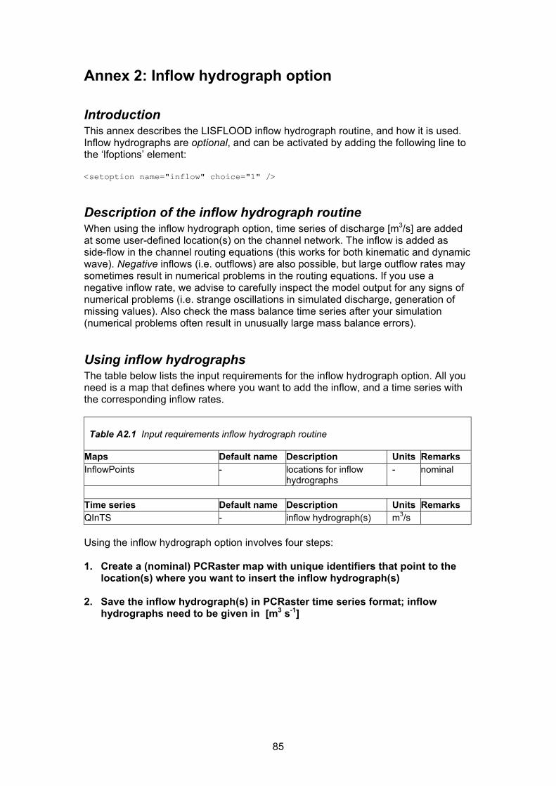
85

Annex 2: Inflow hydrograph option

Introduction This annex describes the LISFLOOD inflow hydrograph routine, and how it is used. Inflow hydrographs are optional, and can be activated by adding the following line to the ‘lfoptions’ element: <setoption name="inflow" choice="1" />

Description of the inflow hydrograph routine When using the inflow hydrograph option, time series of discharge [m3/s] are added at some user-defined location(s) on the channel network. The inflow is added as side-flow in the channel routing equations (this works for both kinematic and dynamic wave). Negative inflows (i.e. outflows) are also possible, but large outflow rates may sometimes result in numerical problems in the routing equations. If you use a negative inflow rate, we advise to carefully inspect the model output for any signs of numerical problems (i.e. strange oscillations in simulated discharge, generation of missing values). Also check the mass balance time series after your simulation (numerical problems often result in unusually large mass balance errors).

Using inflow hydrographs The table below lists the input requirements for the inflow hydrograph option. All you need is a map that defines where you want to add the inflow, and a time series with the corresponding inflow rates.

Table A2.1 Input requirements inflow hydrograph routine

Maps Default name Description Units Remarks InflowPoints - locations for inflow

hydrographs - nominal

Time series Default name Description Units Remarks QInTS - inflow hydrograph(s) m3/s

Using the inflow hydrograph option involves four steps:

1. Create a (nominal) PCRaster map with unique identifiers that point to the

location(s) where you want to insert the inflow hydrograph(s) 2. Save the inflow hydrograph(s) in PCRaster time series format; inflow

hydrographs need to be given in [m3 s-1]

86

IMPORTANT: PCRaster assumes that the first data series in the time series file (i.e. the second column, since the first column contains the time step number) corresponds to unique identifier 1 on the InflowPoints map; the second series to unique identifier 2, and so on. So, even if your InflowPoints map only contains (as an example) identifiers 3 and 4, you still need to include the columns for identifiers 1 and 2!! The best thing to do in such a case is to fill any unused columns with zeroes (0). Also, your inflow hydrograph time series should always start at t=1, even if you set StepStart to some higher value. For more info on time series files please have a look at the PCRaster documentation.

3. Make sure that the names of the map and time series are defined in the

settings file

In the ‘lfuser’ element (replace the file paths/names by the ones you want to use): <group> <comment> ************************************************************** INFLOW HYDROGRAPH (OPTIONAL) ************************************************************** </comment> <textvar name="InflowPoints" value="/floods2/yourhomedir/yourcatchment/maps/inlets.map"> <comment> OPTIONAL: nominal map with locations of (measured) inflow hydrographs [cu m / s] </comment> </textvar> <textvar name="QInTS" value="/floods2/yourhomedir/yourcatchment/inflow/inflow.tss"> <comment> OPTIONAL: observed or simulated input hydrographs as time series [cu m / s] Note that identifiers in time series correspond to InflowPoints map (also optional) </comment> </textvar> </group>

4. Activate the inflow hydrograph option Add the following line to the ‘lfoptions’ element: <setoption name="inflow" choice="1" /> Now you are ready to run the model with the inflow hydrograph.

Substituting subcatchments with measured inflow hydrographs One of the most common uses of the inflow hydrograph option is this: suppose we have a catchment where we only want to simulate the downstream part. If measured time series of discharge are available for the upstream catchment(s), we can use

87

these to represent the inflow into the more downstream part. Figure A2.1 shows an example, where we have measured discharge of subcatchment A (just before it enters the main river). In this case it is important to pay special attention to two issues.

Exclude subcatchments from MaskMap First, make sure that subcatchment A is excluded (i.e. have boolean(0) or missing value) on LISFLOOD’s MaskMap (which defines which pixels are included in the calculations and which are not). If you include it, LISFLOOD will first simulate discharge coming out of subcatchment A, and then add the (measured) inflow on top of it! Of course this doesn’t make any sense, so always be careful which areas are included in your simulation and which are not.

Figure A2.1 Using the inflow hydrograph using measured discharge of subcatchment

A. MaskMap must have boolean(0) (or missing value) for subcatchment A, see text for explanation.

Make sure your inflow points are where you need them If you already have all gauge locations on a PCRaster map, these mostly cannot be used directly as inflow hydrograph locations. The reason is simple: suppose –in our previous example– we know the outflow point of subcatchment A. This point is the most downstream point within that subcatchment. However, the flow out of subcatchment A is actually added to the main river one cell downstream! Also, if we exclude subcatchment A from our simulation (as explained in the foregoing), this means we also exclude the outflow point of that subcatchment. Because of this, inflow points into the main river are usually located one pixel downstream of the

88

outflow points of the corresponding subcatchment. If you already have a (nominal) map of of your subcatchments, a PCRaster script exists that automatically calculates the corresponding out- and inflow points.

89

Annex 3: Dynamic wave option

Introduction This annex describes the LISFLOOD dynamic wave routine, and how it is used. The current implementation of the dynamic wave function in PCRaster is not a complete dynamic wave formulation according to the summary of the Saint Venant equations as discussed in Chow (1988). The implementation currently consists of the friction force term, the gravity force term and the pressure force term and should therefore be correctly characterised as a diffusion wave formulation. The equations are solved as an explicit, finite forward difference scheme. A straightforward iteration using an Euler solution scheme is used to solve these equations. Dynamic wave routing is optional, and can be activated by adding the following line to the ‘lfoptions’ element: <setoption name="dynamicWave" choice="1" />

Time step selection The current dynamic wave implementation requires that all equations are solved using a time step that is much smaller (order of magnitude: seconds-minutes) than the typical overall time step used by LISFLOOD (order of magnitude: hours-day). More specifically, during one (sub) time step no water should be allowed to travel more than 1 cell downstream, i.e.:

ddyn cV

xt+Δ

≤Δ'

where ∆’tdyn is the sub-step for the dynamic wave [seconds], ∆x is the length of one channel element (pixel) [m], V is the flow velocity [m s-1] and cd is dynamic wave celerity [m s-1]. The dynamic wave celerity can be calculated as (Chow, 1988):

gycd = where g is the acceleration by gravity [m s-2] and y is the depth of flow [m]. For a cross-section of a regular geometric shape, y can be calculated from the channel dimensions. Since the current dynamic wave routine uses irregularly shaped cross-section data, we simply assume than y equals the water level above the channel bed. The flow velocity is simply: AQV ch /= where Qch is the discharge in the channel [m3 s-1], and A the cross-sectional area [m2]. The Courant number for the dynamic wave, Cdyn, can now be computed as:

xtcV

C ddyn Δ

Δ+=

)(

where ∆t is the overall model time step [s]. The number of sub-steps is then given by:

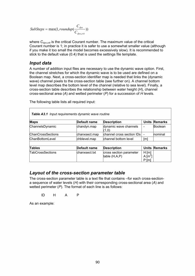
90

))(,1max(,critdyn

dyn

CC

roundupSubSteps =

where Cdyn,crit is the critical Courant number. The maximum value of the critical Courant number is 1; in practice it is safer to use a somewhat smaller value (although if you make it too small the model becomes excessively slow). It is recommended to stick to the default value (0.4) that is used the settings file template.

Input data A number of addition input files are necessary to use the dynamic wave option. First, the channel stretches for which the dynamic wave is to be used are defined on a Boolean map. Next, a cross-section identifier map is needed that links the (dynamic wave) channel pixels to the cross-section table (see further on). A channel bottom level map describes the bottom level of the channel (relative to sea level). Finally, a cross-section table describes the relationship between water height (H), channel cross-sectional area (A) and wetted perimeter (P) for a succession of H levels. The following table lists all required input:

Table A3.1 Input requirements dynamic wave routine

Maps Default name Description Units Remarks ChannelsDynamic chandyn.map dynamic wave channels

(1,0) - Boolean

ChanCrossSections chanxsect.map channel cross section IDs - nominal ChanBottomLevel chblevel.map channel bottom level [m] Tables Default name Description Units Remarks TabCrossSections chanxsect.txt cross section parameter

table (H,A,P) H:[m] A:[m2] P:[m]

Layout of the cross-section parameter table The cross-section parameter table is a text file that contains –for each cross-section- a sequence of water levels (H) with their corresponding cross-sectional area (A) and wetted perimeter (P). The format of each line is as follows:

ID H A P As an example:

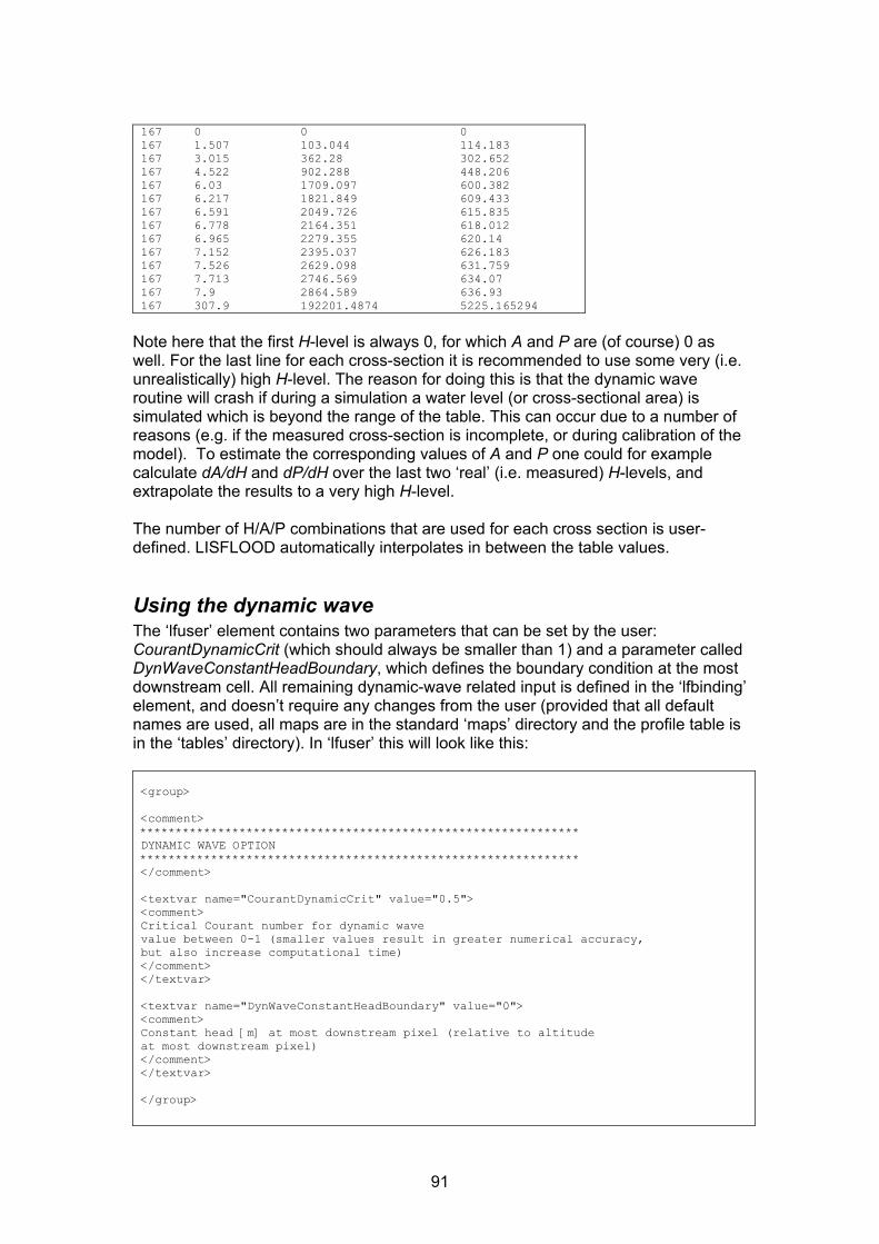
91

167 0 0 0 167 1.507 103.044 114.183 167 3.015 362.28 302.652 167 4.522 902.288 448.206 167 6.03 1709.097 600.382 167 6.217 1821.849 609.433 167 6.591 2049.726 615.835 167 6.778 2164.351 618.012 167 6.965 2279.355 620.14 167 7.152 2395.037 626.183 167 7.526 2629.098 631.759 167 7.713 2746.569 634.07 167 7.9 2864.589 636.93 167 307.9 192201.4874 5225.165294

Note here that the first H-level is always 0, for which A and P are (of course) 0 as well. For the last line for each cross-section it is recommended to use some very (i.e. unrealistically) high H-level. The reason for doing this is that the dynamic wave routine will crash if during a simulation a water level (or cross-sectional area) is simulated which is beyond the range of the table. This can occur due to a number of reasons (e.g. if the measured cross-section is incomplete, or during calibration of the model). To estimate the corresponding values of A and P one could for example calculate dA/dH and dP/dH over the last two ‘real’ (i.e. measured) H-levels, and extrapolate the results to a very high H-level. The number of H/A/P combinations that are used for each cross section is user-defined. LISFLOOD automatically interpolates in between the table values.

Using the dynamic wave The ‘lfuser’ element contains two parameters that can be set by the user: CourantDynamicCrit (which should always be smaller than 1) and a parameter called DynWaveConstantHeadBoundary, which defines the boundary condition at the most downstream cell. All remaining dynamic-wave related input is defined in the ‘lfbinding’ element, and doesn’t require any changes from the user (provided that all default names are used, all maps are in the standard ‘maps’ directory and the profile table is in the ‘tables’ directory). In ‘lfuser’ this will look like this: <group> <comment> ************************************************************** DYNAMIC WAVE OPTION ************************************************************** </comment> <textvar name="CourantDynamicCrit" value="0.5"> <comment> Critical Courant number for dynamic wave value between 0-1 (smaller values result in greater numerical accuracy, but also increase computational time) </comment> </textvar> <textvar name="DynWaveConstantHeadBoundary" value="0"> <comment> Constant head [m] at most downstream pixel (relative to altitude at most downstream pixel) </comment> </textvar> </group>

92

93

Annex 4: Polder option

Introduction This annex describes the LISFLOOD polder routine, and how it is used. The simulation of polders is optional, and it can be activated by adding the following line to the ‘lfoptions’ element: <setoption name="simulatePolders" choice="1" /> Polders can be simulated on channel pixels where dynamic wave routing is used. The routine does not work for channel stretches where the kinematic wave is used!

Description of the polder routine Polders are simulated as points in the channel network. The polder routine is adapted from Förster et. al (2004), and based on the weir equation of Poleni (Bollrich & Preißler, 1992). The flow rates from the channel to the polder area and vice versa are calculated by balancing out the water levels in the channel and in the polder, as shown in Figure A4.1.

Figure A4.1 Schematic overview of the simulation of polders. pb is the polder

bottom level (above the channel bottom); wc is the water level in the channel; hc and hp are the water levels above the polder in- / outflow, respectively

From the Figure, it is easy to see that there can be three situations:

1. hc > hp: water flows out of the channel, into the polder. The flow rate, qc,p, is calculated using:

16

23

,

1

;2

⎥⎦

⎤⎢⎣

⎡−=

=

c

p

cpc

hh

c

hgcbq μ

(A4.1)

where b is the outflow width [m], g is the acceleration due to gravity (9.81 m s-

2) and μ is a weir constant which has a value of 0.49. Furthermore qc,p is in [m3 s-1].

94

2. hc < hp: water flows out of the polder back into the channel. The flow rate, qp,c,

is now calculated using:

16

23

,

1

;2

⎥⎥⎦

⎤

⎢⎢⎣

⎡−=

=

p

c

pcp

hhc

hgcbq μ

(A4.2)

3. hc = hp: no water flowing into either direction (note here that the minimum value of hc is zero). In this case both qc,p and qp,c are zero.

Regulated and unregulated polders The above equations are valid for unregulated polders. It is also possible to simulated regulated polders, which is illustrated in Figure A4.2. Regulated polders are opened at a user-defined time (typically during the rising limb of a flood peak). The polder closes automatically once it is full. Subsequently, the polder is opened again to release the stored water back into the channel, which also occurs at a user-defined time. The opening- and release times for each polder are defined in two lookup tables (see Table 4.1). In order to simulate the polders in unregulated mode these times should both be set to a bogus value of -9999. Only if both opening- and release time are set to some other value, LISFLOOD will simulate a polder in regulated mode. Since LISFLOOD only supports one single regulated open-close-release cycle per simulation, you should use regulated mode only for single flood events. For continuous simulations (e.g. long-tem waterbalance runs) you should only run the polders in unregulated mode.

95

Figure A4.2 Simulation of a regulated polder. Polder is closed (inactive) until

user-defined opening time, after which it fills up to its capacity (flow rate according to Eq A4.1). Water stays in polder until user-defined release time, after which water is released back to the channel (flow rate according to Eq A4.2).

Preparation of input data The locations of the reservoirs are defined on a (nominal) map called ‘polders.map’. Any polders that are not on a channel pixel are ignored by LISFLOOD, so you may want to check the polder locations before running the model (you can do this by displaying the reservoirs map on top of the channel map). The current implementation of the polder routine may result in numerical instabilities for kinematic wave pixels, so for the moment it is recommended to define polders only on channels where the dynamic wave is used. Furthermore, the properties of each polder are described using a number of tables. All required input is listed in the following table:

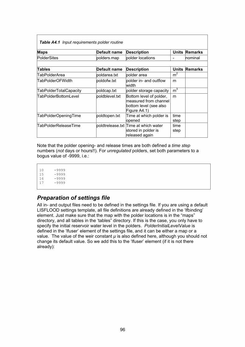
96

Table A4.1 Input requirements polder routine

Maps Default name Description Units Remarks PolderSites polders.map polder locations - nominal Tables Default name Description Units Remarks TabPolderArea poldarea.txt polder area m2

TabPolderOFWidth poldofw.txt polder in- and outflow width

m

TabPolderTotalCapacity poldcap.txt polder storage capacity m3 TabPolderBottomLevel poldblevel.txt Bottom level of polder,

measured from channel bottom level (see also Figure A4.1)

m

TabPolderOpeningTime poldtopen.txt Time at which polder is opened

time step

TabPolderReleaseTime poldtrelease.txt Time at which water stored in polder is released again

time step

Note that the polder opening- and release times are both defined a time step numbers (not days or hours!!). For unregulated polders, set both parameters to a bogus value of -9999, i.e.: 10 -9999 15 -9999 16 -9999 17 -9999

Preparation of settings file All in- and output files need to be defined in the settings file. If you are using a default LISFLOOD settings template, all file definitions are already defined in the ‘lfbinding’ element. Just make sure that the map with the polder locations is in the “maps” directory, and all tables in the ‘tables” directory. If this is the case, you only have to specify the initial reservoir water level in the polders. PolderInitialLevelValue is defined in the ‘lfuser’ element of the settings file, and it can be either a map or a value. The value of the weir constant μ is also defined here, although you should not change its default value. So we add this to the ‘lfuser’ element (if it is not there already):

97

<group> <comment> ************************************************************** POLDER OPTION ************************************************************** </comment> <textvar name="mu" value="0.49"> <comment> Weir constant [-] (Do not change!) </comment> </textvar> <textvar name="PolderInitialLevelValue" value="0"> <comment> Initial water level in polder [m] </comment> </textvar> </group>

To switch on the polder routine, add the following line to the ‘lfoptions’ element: <setoption name="simulatePolders" choice="1" /> Now you are ready to run the model. If you want to compare the model results both with and without the inclusion of polders, you can switch off the simulation of polders either by:

3. Removing the ‘simulatePolders’ statement from the ‘lfoptions element, or 4. changing it into <setoption name="simulatePolders" choice="0" />

Both have exactly the same effect. You don’t need to change anything in either ‘lfuser’ or ‘lfbinding’; all file definitions here are simply ignored during the execution of the model.

Polder output files The polder routine produces 2 additional time series and one map (or stack of maps, depending on the value of LISFLOOD variable ReportSteps), as listed in the following table:

98

Table A4.2 Output of polder routine

Maps Default name Description Units Remarks PolderLevelState hpolxxxx.xxx water level in polder at

last time step12 m

Time series Default name Description Units Remarks PolderLevelTS hPolder.tss water level in polder (at

polder locations) m

PolderFluxTS qPolder.tss Flux into and out of polder (positive for flow from channel to polder, negative for flow from polder to channel)

m3/s

Note that you can use the map with the polder level at the last time step to define the initial conditions of a succeeding simulation, e.g.: <textvar name="PolderInitialLevelValue" value="/mycatchment/hpol0000.730">

Limitations For the moment, polders can be simulated on channel pixels where dynamic wave routing is used. For channels where the kinematic wave is used, the routine will not work and may lead to numerical instabilities or even model crashes. This limitation may be resolved in future model versions.

12 xxx represents the number of the last time step; e.g. for a 730-step simulation the name will be ‘hpol0000.730’, and so on.

99

Annex 5: Simulation of lakes

Introduction This annex describes the LISFLOOD lake routine, and how it is used. The simulation of lakes is optional, and it can be activated by adding the following line to the ‘lfoptions’ element: <setoption name="simulateLakes" choice="1" /> Lakes can be simulated on channel pixels where kinematic wave routing is used. The routine does not work for channel stretches where the dynamic wave is used!

Description of the lake routine Lakes are simulated as points in the channel network. Figure A5.1 shows all computed in- and outgoing fluxes. Lake inflow equals the channel flow upstream of the lake location. The flow out of the lake is computed using the following rating curve (e.g. Maidment, 1992):

Blake HHAO )( 0−=

Olake : Lake outflow rate [m3 s-1] H : Water level in lake [m] H0 : Water level at which lake outflow is zero [m] A, B : Constants [-]

.

Figure A5.1 Schematic overview of the simulation of lakes. H0 is the water

level at which the outflow is zero; H is the water level in the lake and EW is the evaporation from the lake

100

Both H and H0 can be defined relative to an arbitrary reference level. Since the outflow is a function of the difference between both levels, the actual value of this reference level doesn’t matter if H > H0. However, it is advised to define both H and H0 relative to the average bottom level of the lake. This will result in more realistic simulations during severe drought spells, when the water level drops below H0 (in which case lake outflow ceases). The value of constant A can be approximated by the width of the lake outlet in meters, and B is within the range 1.5-2 (reference?). Lake evaporation occurs at the potential evaporation rate of an open water surface.

Initialisation of the lake routine Because lakes (especially large ones) tend to produce a relatively slow response over time, it is important to make sure that the initial lake level is set to a more or less sensible value. Just as is the case with the initialisation of the lower groundwater zone, LISFLOOD has a special option that will compute a steady-state lake level and use this as the initial value. The steady-state level is computed from the water balance of the lake. If Vl is the total lake volume [m3], the rate of change of Vl at any moment is given by the continuity equation:

)()( tOtIdtdVl −=

where I and O are the in- and outflow rates, respectively. For a steady-state situation the storage remains constant, so:

0)()(0 =−⇔= tOtIdtdVl

Substituting all in- and outflow terms gives:

0)( 0 =−−− Bll HHAEWI

where Il is the inflow into the lake and EWl the lake evaporation (both expressed in m3 s-1). Re-arranging gives the steady-state lake level:

B

llss A

EWIHH1

0 ⎟⎠⎞

⎜⎝⎛ −

+=

LISFLOOD calculates the steady-state lake level based on a user-defined average net inflow (=Il – EWl). The average net inflow can be estimated using measured discharge and evaporation records. If measured discharge is available just downstream of the lake (i.e. the outflow), the (long-term) average outflow can be used as the net inflow estimate (since, for a steady state situation, inflow equals outflow). If only inflow is available, all average inflows should be summed, and the average lake evaporation should be subtracted from this figure. Table A5.1 gives a worked example. Be aware that the calculation can be less straightforward for very large lakes with multiple inlets (which are not well represented by the current point approach anyway).

101

Table A5.1: Calculation of average net lake inflow Lake characteristics lake area: 215•106 m2

mean annual discharge downstream of lake: 293 m3 s-1 mean annual discharge upstream of lake: 300 m3 s-1 mean annual evaporation: 1100 mm yr-1 Calculation of average net inflow METHOD 1: USING AVERAGE OUTFLOW assuming lake is in quasi steady-state:

average net inflow = average net outflow = 293 m3 s-1 METHOD 2: USING AVERAGE INFLOW AND EVAPORATION Only use this method if no outflow data are available

1. Express lake evaporation in m3 s-1:

1100 mm yr-1 / 1000 = 1.1 m yr-1 1.1 m yr-1 x 215•106 m2 = 2.37•108 m3 yr-1 2.37•108 m3 yr-1 / (365 days x 86400 seconds) = 7.5 m3 s-1

2. Compute net inflow: net inflow = 300 m3 s-1 – 7.5 m3 s-1 = 292.5 m3 s-1

Preparation of input data The lake locations defined on a (nominal) map called ‘lakes.map’. It is important that all reservoirs are located on a channel pixel (you can verify this by displaying the reservoirs map on top of the channel map). Also, since each lake receives its inflow from its upstream neighbouring channel pixel, you may want to check if each lake has any upstream channel pixels at all (if not, the lake will just gradually empty during a model run!). The lake characteristics are described by 4 tables. Table 5.2 lists all required input. When you create the map with the lake locations, pay special attention to the following: if a lake is located on the most downstream cell (i.e. the outflow point, see Figure A5.2), the lake routine may produce erroneous output. In particular, the mass balance errors cannot be calculated correctly in that case. The same applies if you simulate only a sub-catchment of a larger map (by selecting the subcatchment in the mask map). This situation can usually be avoided by extending the mask map by one cell in downstream direction.

102

Table A5.2 Input requirements lake routine

Maps Default name Description Units Remarks LakeSites lakes.map lake locations - nominal Tables Default name Description Units Remarks TabLakeArea lakearea.txt lake surface area m2

TabLakeH0 lakeh0.txt water level at which lake outflow is zero

m relative to average lake bottom level

TabLakeA lakea.txt lake parameter A - ≈ outlet width in meters

TabLakeB lakeb.txt lake parameter B - 1.5-2

Figure A5.2 Placement of the lakes: lakes on the outflow point (left) result in

erroneous behavior of the lake routine.

Preparation of settings file All in- and output files need to be defined in the settings file. If you are using a default LISFLOOD settings template, all file definitions are already defined in the ‘lfbinding’ element. Just make sure that the map with the lake locations is in the “maps” directory, and all tables in the ‘tables” directory. If this is the case, you only have to specify the initial lake level and –if you are using the steady-state option- the mean net lake inflow (make this a map if you’re simulating multiple lakes simultaneously). Both can be set in the ‘lfuser’ element. LakeInitialLevelValue can be either a map or a single value. Setting LakeInitialLevelValue to -9999 will cause LISFLOOD to calculate the steady-state level. So we add this to the ‘lfuser’ element (if it is not there already):

103

<group> <comment> ************************************************************** LAKE OPTION ************************************************************** </comment> <textvar name="LakeInitialLevelValue" value="-9999"> <comment> Initial lake level [m] -9999 sets initial value to steady-state level </comment> </textvar> <textvar name="LakeAvNetInflowEstimate" value="292.5"> <comment> Estimate of average net inflow into lake (=inflow – evaporation) [cu m / s] Used to calculated steady-state lake level in case LakeInitialLevelValue is set to -9999 </comment> </textvar> </group>

Finally, you have to tell LISFLOOD that you want to simulate lakes! To do this, add the following statement to the ‘lfoptions’ element: <setoption name="simulateLakes" choice="1" /> Now you are ready to run the model. If you want to compare the model results both with and without the inclusion of lakes, you can switch off the simulation of lakes either by:

5. Removing the ‘simulateLakes’ statement from the ‘lfoptions element, or 6. changing it into <setoption name="simulateLakes" choice="0" />

Both have exactly the same effect. You don’t need to change anything in either ‘lfuser’ or ‘lfbinding’; all file definitions here are simply ignored during the execution of the model.

Lake output files The lake routine produces 4 additional time series and one map (or stack), as listed in the following table:

104

Table A5.3 Output of lake routine

Maps Default name Description Units Remarks LakeLevelState lakhxxxx.xxx lake level at last time

step13 m

Time series Default name Description Units Remarks LakeInflowTS qLakeIn.tss inflow into lakes m3/s

LakeOutflowTS qLakeOut.tss flow out of lakes m3/s LakeEWTS EWLake.tss lake evaporation mm LakeLevelTS hLake.tss lake level m Note that you can use the map with the lake level at the last time step to define the initial conditions of a succeeding simulation, e.g.: <textvar name="LakeInitialLevelValue" value="/mycatchment/lakh0000.730">

13 xxx represents the number of the last time step; e.g. for a 730-step simulation the name will be ‘lakh0000.730’, and so on.

105

Annex 6: Simulation and reporting of water levels

Introduction Within LISFLOOD it is possible to simulate and report water levels in the channel. The simulation of water levels is optional, and it can be activated by adding the following line to the ‘lfoptions’ element: <setoption name="simulateWaterLevels" choice="1" /> If the option is switched on, water levels are calculated for channel pixels where either kinematic or dynamic wave routing is used. Using this option does not influence the actual model results in any way, and it is included only to allow the model user to report water levels. The actual reporting of the simulated water levels (as time series or maps) can be activated using two separate options.

Calculation of water levels For channel stretches that are simulated using the dynamic wave, the water level in the channel is simply the difference between the channel head and the channel bottom level. For kinematic wave stretches, only approximate water levels can be estimated from the cross-sectional (wetted) channel area, Ach for each time step. Since the channel cross-section is described as a trapezoid, water levels follow directly from Ach , channel bottom width, side slope and bankfull level. If Ach exceeds the bankfull cross-sectional area (Abf), the surplus is distributed evenly over the (rectangular) floodplain, and the depth of water on the floodplain is added to the (bankfull) channel depth. Figure A6.1 below further illustrates the cross-section geometry. All water levels are relative to channel bottom level (zbot in the Figure).

Figure A6.1 Geometry of channel cross-section in kinematic wave routing.

Wb: channel bottom width; Wu: channel upper width; zbot: channel bottom level; zfp: floodplain bottom level; s: channel side slope; Wfp: floodplain width; Abf: channel cross-sectional area at bankfull; Afp: floodplain cross-sectional area; Dbf: bankfull channel depth, Dfp: depth of water on the floodplain

106

In order to calculate water levels, LISFLOOD needs a map with the with of the floodplain in [m], which is defined by ‘lfbinding’ variable FloodPlainWidth (the default name of this map is chanfpln.map).

Reporting of water levels Water levels can be reported as time series (at the gauge locations that are also used for reporting discharge), or as maps. To generate a time series, add the following line to the ‘lfoptions’ element of your settings file: <setoption name="repWaterLevelTs" choice="1" /> For maps, use the following line instead: <setoption name="repWaterLevelMaps" choice="1" /> In either case, the reporting options should be used in addition to the ‘simulateWaterLevels’ option. If you do not include the ‘simulateWaterLevels’ option, there will be nothing to report and LISFLOOD will exit with an error message.

Preparation of settings file The naming of the reported water level time series and maps is defined in the settings file. If you are using a default LISFLOOD settings template, all file definitions are already defined in the ‘lfbinding’ element. Time series: <textvar name="WaterLevelTS" value="$(PathOut)/waterLevel.tss"> <comment> Reported water level [m] </comment> </textvar>

Map stack: <textvar name="WaterLevelMaps" value="$(PathOut)/wl"> <comment> Reported water level [m] </comment> </textvar>

107

Annex 7: Simulation and reporting of soil moisture as pF values

Introduction LISFLOOD offers the possibility to calculate pF values from the moisture content of both soil layers. The calculation of pF values is optional, and it can be activated by adding the following line to the ‘lfoptions’ element: <setoption name="simulatePF" choice="1" /> Using this option does not influence the actual model results in any way, and it is included only to allow the model user to report pF time series or maps. The actual reporting of the computed pF values (as time series or maps) can be activated using separate options (which are discussed further on).

Calculation of pF A soil’s pF is calculated as the logarithm of the capillary suction head, h:

)(log10 hpF = with h in [cm] (positive upwards). Values of pF are typically within the range 1.0 (very wet) to 5.0 (very dry). The relationship between soil moisture status and capillary suction head is described by the Van Genuchten equation (here again re-written in terms of mm water slice, instead of volume fractions):

nm

r

rs

wwwwh

/1/1

11⎥⎥⎦

⎤

⎢⎢⎣

⎡−⎟⎟

⎠

⎞⎜⎜⎝

⎛−−

=α

where h is the suction head [cm], and w, wr and ws are the actual, residual and maximum amounts of moisture in the soil respectively (all in [mm]). Parameter α is related to soil texture. Parameters m and n are calculated from the pore-size index, λ (which is related to soil texture as well):

1+=λλm

1+= λn

If the soil contains no moisture at all (w=0), h is set to a fixed (arbitrary) value of 1·107 cm.

108

Reporting of pF pF can be reported as time series (at the locations defined on the “sites” map or as average values upstream each gauge location), or as maps. To generate time series at the “sites”, add the following line to the ‘lfoptions’ element of your settings file: <setoption name="repPFTs" choice="1" /> For maps, use the following lines instead (for the upper and lower soil layer, respectively): <setoption name="repPF1Maps" choice="1" /> <setoption name="repPF2Maps" choice="1" /> In either case, the reporting options should be used in addition to the ‘simulatePF’ option. If you do not include the ‘simulatePF’ option, there will be nothing to report and LISFLOOD will exit with an error message.

Preparation of settings file The naming of the reported time series and maps is defined in the settings file. Tables A7.1 and A7.2 list the settings variables default output names. If you are using a default LISFLOOD settings template, all file definitions are already defined in the ‘lfbinding’ element. Time series: <comment> PF TIMESERIES, VALUES AT SITES </comment> <textvar name="PF1TS" value="$(PathOut)/pFTop.tss"> <comment> Reported pF upper soil layer [-] </comment> </textvar> <textvar name="PF2TS" value="$(PathOut)/pFSub.tss"> <comment> Reported pF lower soil layer [-] </comment> </textvar> <comment> PF TIMESERIES, AVERAGE VALUES UPSTREAM OF GAUGES </comment> <textvar name="PF1AvUpsTS" value="$(PathOut)/pFTopUps.tss"> <comment> Reported pF upper soil layer [-] </comment> </textvar> <textvar name="PF2AvUpsTS" value="$(PathOut)/pFSubUps.tss"> <comment> Reported pF lower soil layer [-] </comment> </textvar>

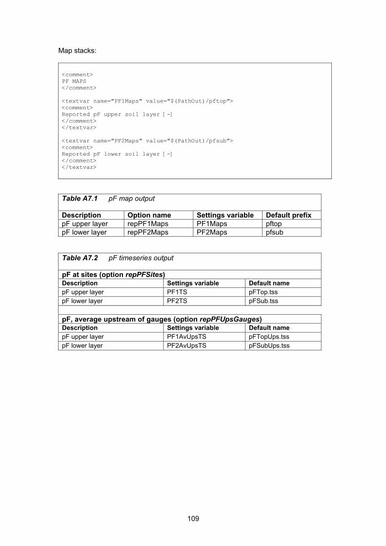
109

Map stacks: <comment> PF MAPS </comment> <textvar name="PF1Maps" value="$(PathOut)/pftop"> <comment> Reported pF upper soil layer [-] </comment> </textvar> <textvar name="PF2Maps" value="$(PathOut)/pfsub"> <comment> Reported pF lower soil layer [-] </comment> </textvar>

Table A7.1 pF map output Description Option name Settings variable Default prefix pF upper layer repPF1Maps PF1Maps pftop pF lower layer repPF2Maps PF2Maps pfsub

Table A7.2 pF timeseries output pF at sites (option repPFSites) Description Settings variable Default name pF upper layer PF1TS pFTop.tss pF lower layer PF2TS pFSub.tss pF, average upstream of gauges (option repPFUpsGauges) Description Settings variable Default name pF upper layer PF1AvUpsTS pFTopUps.tss pF lower layer PF2AvUpsTS pFSubUps.tss

European Commission EUR 22166 EN/2 –Joint Research Centre –Institute for Environment and Sustainability Title: LISFLOOD - Distributed Water Balance and Flood Simulation Model. Revised User Manual Authors: Johan van der Knijff, Ad de Roo Luxembourg: Office for Official Publications of the European Communities 2008 – 109 pp. – 21 x 27.9 cm EUR - Scientific and Technical Research series; ISSN 1018-5593 Abstract The revised LISFLOOD User Manual documents the LISFLOOD water balance and flood simulation model. The first part of this document gives a detailed description of the characteristics of the LISFLOOD model, focusing on process descriptions and the governing equations. The second part covers all practical LISFLOOD issues, such as installing the model, setting up the necessary input data and running it.

How to obtain EU publications Our priced publications are available from EU Bookshop (http://bookshop.europa.eu), where you can place an order with the sales agent of your choice. The Publications Office has a worldwide network of sales agents. You can obtain their contact details by sending a fax to (352) 29 29-42758.

The mission of the JRC is to provide customer-driven scientific and technical support for the conception, development, implementation and monitoring of EU policies. As a service of the European Commission, the JRC functions as a reference centre of science and technology for the Union. Close to the policy-making process, it serves the common interest of the Member States, while being independent of special interests, whether private or national.