Embed Size (px)
Citation preview

Distributed System Design: An Overview*
Jie WuDepartment of Computer and
Information SciencesTemple University
Philadelphia, PA 19122
*Part of the materials come from Distributed System Design, CRC Press, 1999. (Chinese Edition, China Machine Press, 2001.)

The Structure of Classnotes
Focus Example Exercise Project

Table of Contents
Introduction and Motivation Theoretical Foundations Distributed Programming Languages Distributed Operating Systems Distributed Communication Distributed Data Management Reliability Applications Conclusions Appendix

Development of Computer Technology
1950s: serial processors 1960s: batch processing 1970s: time-sharing 1980s: personal computing 1990s: parallel, network, and distributed processing 2000s: wireless networks 2010s: mobile and cloud (edge, fog) computing 2020s: IoT, big data (AI), and blockchain (security)
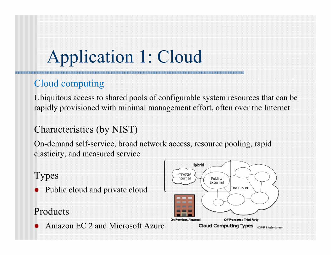
Application 1: CloudCloud computingUbiquitous access to shared pools of configurable system resources that can be rapidly provisioned with minimal management effort, often over the Internet
Characteristics (by NIST)On-demand self-service, broad network access, resource pooling, rapid elasticity, and measured service
Types Public cloud and private cloud
Products Amazon EC 2 and Microsoft Azure

Fog: distributed cloudEdge: devices at the edge network (e.g., Internet of Things IoT)
Fog: distributed cloud (e.g. cloud + IoT) Reduce data communication and process demands Data storage and processing outside the cloud
Products Cisco Cloudlets (CMU) Micro datacenter in Azure

Application 2: HadoopApache Hadoop is built for Big Data processing MapReduce: map, shuffle, and reduce
• Pipeline• Data parallelism
HDFS (Hadoop distributed file systems)
Apache HIVE • Data warehouse• SQL-like interface (distributed database)

SPARK: beyond HadoopApache Spark is built for speed, mainly for ML
• Speed (10x to 100x compared to Hadoop)• Data in memory (Hadoop in hard disk)• RDD: resilient distributed dataset (extension from distributed shared
memory, DSM and fault tolerance)• Streaming• Better API
New paradigm for reinforcement learning (RL)• Stanford DAWN• Berkeley Ray
* gray color: concepts to be covered in this class

Shuffle
TeraSort: map-shuffle-reduce
Map-Shuffle-ReduceMap and Reduce: CPU-intensiveShuffle: I/O-intensive
TeraSortMap: sample & partition dataShuffle: partitioned data
Reduce: locally sort data
Data partition
Map Reduce
Local sort
Data partition
Local sort

Application 3: Bitcoin
Bitcoin: crytocurrency and worldwide payment system First decentralized digital currency without a central bank or
single administrator Transactions: use of cryptograph and is recorded in a
distributed ledger called blockchain
Most crowded trade in 2017: prices go higher not by percentages but multiples
Blockchain: building block
Blockchain: distributed database on a set of communicating nodes
A continuously growing list of records (transactions), called blocks. Transactions: input node(s) to output node(s) Mining: distributed book-keeping to ensure consistency,
complete, and unalterable (using linear cryptograph hash chain)
Byzantine fault tolerance and decentralized consensus

Decentralized ledger in P2P: block chain
User: broadcast transfer
Miner: complete through a random process to get bitcoin
(1) validate, (2) find a key (puzzle solving), and (3) broadcast result
Security: digital signature, hash of previous data
Money transfer: ledger and minor
A B
C
A=$5
$3:A->B
$1:B->C
$3
miner: copy of ledger(invalid)
$3 $1
miner

A distributed system is a collection of independent computers that appear to the users of the system as a single computer.
Distributed systems are "seamless": the interfaces among functional units on the network are for the most part invisible to the user.
System structure from the physical (a) or logical point of view (b).
A Simple Definition

Motivation
People are distributed, information is distributed (Internet and Intranet)
Performance/cost Information exchange and resource sharing (WWW and
CSCW) Flexibility and extensibility Dependability
Two Main Stimuli Technological change User needs

Goals Transparency: hide the fact that its processes and resources
are physically distributed across multiple computers. Access Location Migration Replication Concurrency Failure Persistence
Scalability: in three dimensions Size Geographical distance Administrative structure

Goals (Cont’d.)
Heterogeneity (mobile code and mobile agent) Networks Hardware Operating systems and middleware Program languages
Openness Security Fault Tolerance Concurrency

Scaling Techniques
Latency hiding (pipelining and interleaving execution) Distribution (spreading parts across the system) Replication (caching)

Example 1: (Scaling Through Distribution)
URL searching based on hierarchical DNS name space (partitioned into zones).
DNS name space.

Design Requirements Performance Issues
Responsiveness Throughput Load Balancing
Quality of Service Reliability Security Performance
Dependability Correctness Security Fault tolerance

Similar and Related Concepts
Distributed Network Parallel Concurrent Decentralized

Schroeder's Definition
A list of symptoms of a distributed system Multiple processing elements (PEs) Interconnection hardware PEs fail independently Shared states

Focus 1: Enslow's Definition
Distributed system = distributed hardware + distributed control + distributed data
A system could be classified as a distributed system if all three categories (hardware, control, data) reach a certain degree of decentralization.

Focus 1 (Cont’d.)
Enslow's model of distributed systems.

Hardware
A single CPU with one control unit. A single CPU with multiple ALUs (arithmetic and logic
units).There is only one control unit. Separate specialized functional units, such as one CPU with
one floating-point co-processor. Multiprocessors with multiple CPUs but only one single I/O
system and one global memory. Multicomputers with multiple CPUs, multiple I/O systems
and local memories.

Control Single fixed control point. Note that physically the system
may or may not have multiple CPUs. Single dynamic control point. In multiple CPU cases the
controller changes from time to time among CPUs. A fixed master/slave structure. For example, in a system with
one CPU and one co-processor, the CPU is a fixed master and the co-processor is a fixed slave.
A dynamic master/slave structure. The role of master/slave is modifiable by software.
Multiple homogeneous control points where copies of the same controller are used.
Multiple heterogeneous control points where different controllers are used.

Data Centralized databases with a single copy of both files and
directory. Distributed files with a single centralized directory and no
local directory. Replicated database with a copy of files and a directory at
each site. Partitioned database with a master that keeps a complete
duplicate copy of all files. Partitioned database with a master that keeps only a complete
directory. Partitioned database with no master file or directory.

Network Systems
Performance scales on throughput (transaction response time or number of transactions per second) versus load.
Work on burst mode. Suitable for small transaction-oriented programs (collections
of small, quick, distributed applets). Handle uncoordinated processes.

Parallel Systems
Performance scales on elapsed execution times versus number of processors (subject to either Amdahl or Gustafson law).
Works on bulk mode. Suitable for numerical applications (such as SIMD or SPMD
vector and matrix problems). Deal with one single application divided into a set of
coordinated processes.

Distributed Systems
A compromise of network and parallel systems.

Comparison
Comparison of three different systems.
Item Network sys. Distributed sys. Multiprocessors
Like a virtual uniprocessor
No Yes Yes
Run the same operating system
No Yes Yes
Copies of the operating system
N copies N copies 1 copy
Means of communication
Shared files Messages Shared files
Agreed up network protocols?
Yes Yes No
A single run queue No Yes Yes
Well defined file sharing
Usually no Yes Yes

Focus 2: Different Viewpoints
Architecture viewpoint Interconnection network viewpoint Memory viewpoint Software viewpoint System viewpoint

Architecture Viewpoint
Multiprocessor: physically shared memory structure Multicomputer: physically distributed memory structure.

Interconnection Network Viewpoint
static (point-to-point) vs. dynamics (ones with switches). bus-based (Fast Ethernet) vs. switch-based (routed instead of
broadcast).

Interconnection Network Viewpoint (Cont’d.)
Examples of dynamic interconnection networks: (a) shuffle-exchange, (b) crossbar, (c) baseline, and (d) Benes.
Interconnection Network Viewpoint (Cont’d.)
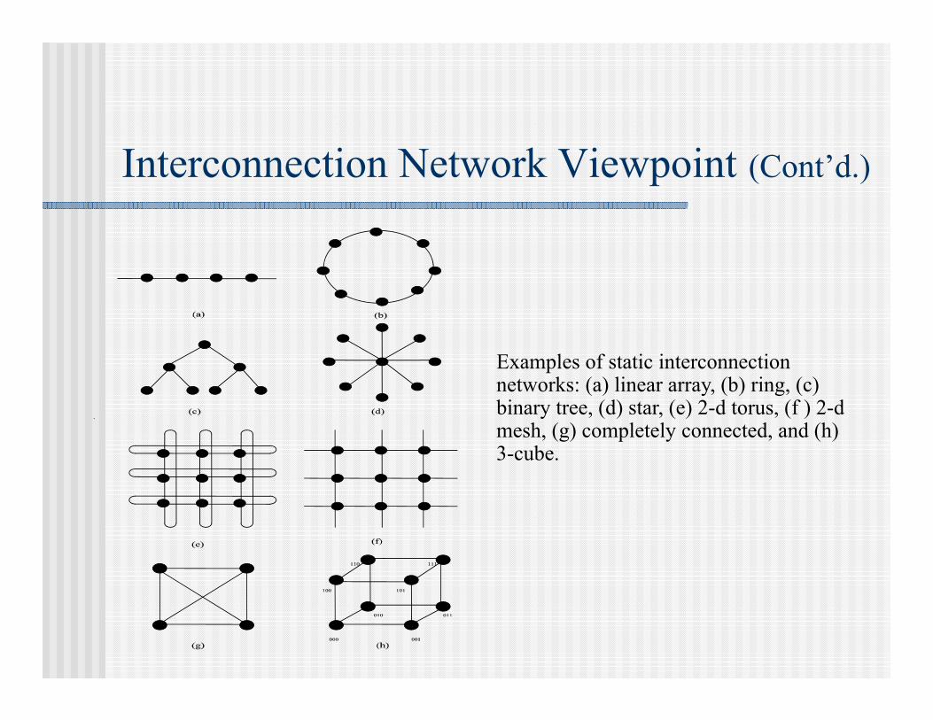
Examples of static interconnection networks: (a) linear array, (b) ring, (c) binary tree, (d) star, (e) 2-d torus, (f ) 2-d mesh, (g) completely connected, and (h) 3-cube.

Measurements for Interconnection Networks
Node degree. The number of edges incident on a node. Diameter. The maximum shortest path between any two
nodes. Bisection width. The minimum number of edges along a cut
which divides a given network into equal halves.

What's the Best Choice? (Siegel 1994) A compiler-writer prefers a network where the transfer time
from any source to any destination is the same to simplify the data distribution.
A fault-tolerant researcher does not care about the type of network as long as there are three copies for redundancy.
A European researcher prefers a network with a node degree no more than four to connect Transputers.

What's the Best Choice? (Cont’d.)
A college professor prefers hypercubes and multistage networks because they are theoretically wonderful.
A university computing center official prefers whatever network is least expensive.
A NSF director wants a network which can best help deliver health care in an environmentally safe way.
A Farmer prefers a wormhole-routed network because the worms can break up the soil and help the crops!

Memory Viewpoint
Physically versus logically shared/distributed memory.

Software Viewpoint
Distributed systems as resource managers like traditional operating systems. Multiprocessor/Multicomputer OS Network OS Middleware (on top of network OS)

Service Common to Many Middleware Systems
High level communication facilities (access transparency)
Naming Special facilities for storage (integrated database)
Middleware

System Viewpoint
The division of responsibilities between system components and placement of the components.

Client-Server Model
multiple servers proxy servers and caches
(a) Client and server and (b) proxy server.

Peer Processes
Peer processes.
Peer-to-Peer: P2P

Mobile Code and Mobile Agents
Mobile code (web applets).

Theoretical foundations Reliability Privacy and security Design tools and methodology Distribution and sharing Accessing resources and services User environment Distributed databases Network research
Key Issues (Stankovic's list)

Wu's Book
Distributed Programming Languages Basic structures
Theoretical Foundations Global state and event ordering Clock synchronization
Distributed Operating Systems Mutual exclusion and election Detection and resolution of deadlock self-stabilization Task scheduling and load balancing
Distributed Communication One-to-one communication Collective communication

Wu's Book (Cont’d.)
Reliability Agreement Error recovery Reliable communication
Distributed Data Management Consistency of duplicated data Distributed concurrency control
Applications Distributed operating systems Distributed file systems Distributed database systems Distributed shared memory Distributed heterogeneous systems
Wu's Book (Cont’d.)
Part 1: Foundations and Distributed Algorithms Part 2: System infrastructure Part 3: Applications

What is Distributed Algorithms
Parallel Computing: efficiency Real-Time: On-time computing Distributed Computing: uncertainty
Simplicity, elegance, and beauty are first-class citizens(Michel Raynal, 2013)

Distributed Message-Passing Algorithms
Termination In a social network, each person exchanges his/her friend
list with friends. What is the stoppage condition?
Global State How to design an observation algorithm by observing an
execution without modifying its behavior?
Distributed Consensus How to reach distributed consensus (e.g., binary
decisions) in the presence of traitors?

Distributed Message-Passing Algorithms
Logical Clock How to order events in different systems with
asynchronous clocks? How to discard obsolete data?
Data How to replicate data and keep them consistent?
Load How to distribute load in a load balanced way?
Routing How to perform efficient routing that is deadlock-free
and fault-tolerant?

References IEEE Transactions on Parallel and Distributed Systems
(TPDS) Journal of Parallel and Distributed Computing (JPDC) Distributed Computing IEEE International Conference on Distributed Computing
Systems (ICDCS) IEEE International Conference on Reliable Distributed
Systems (SRDS) ACM Symposium on Principles of Distributed Computing
(PODC) IEEE Concurrency (formerly IEEE Parallel & Distributed
Technology: Systems & Applications)
Exercise 1
1. In your opinion, what is the future of the computing and the field of distributed systems?
2. Use your own words to explain the differences between distributed systems, multiprocessors, and network systems.
3. Calculate (a) node degree, (b) diameter, (c) bisection width, and (d) the number of links for an n x n 2-d mesh, an n x n 2-d torus, and an n-dimensional hypercube.

Table of Contents Introduction and Motivation Theoretical Foundations Distributed Programming Languages Distributed Operating Systems Distributed Communication Distributed Data Management Reliability Applications Conclusions Appendix

State Model
A process executes three types of events: internal actions, send actions, and receive actions.
A global state (also configuration): a collection of local states and the state of all the communication channels.
Global state evolves bymeans of transitions
Initiator: first event Distributed algorithm:
multiple initiatorsSystem structure from logical point of view.

Thread
lightweight process (maintain minimum information in its context)
multiple threads of control per process multithreaded servers (vs. single-threaded process)
A multithreaded server in a dispatcher/worker model.
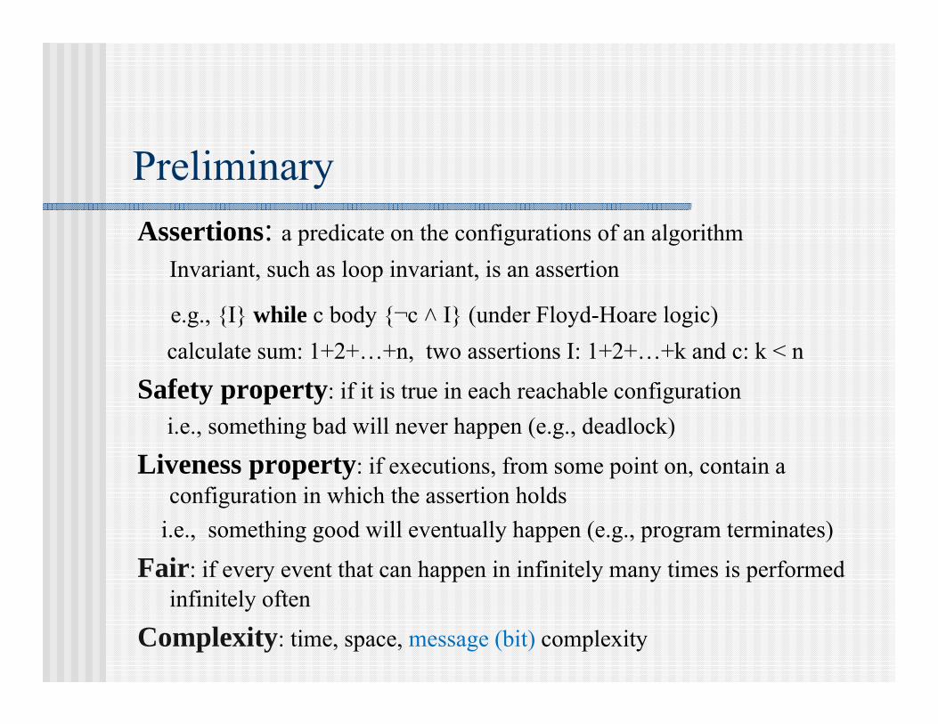
PreliminaryAssertions: a predicate on the configurations of an algorithm
Invariant, such as loop invariant, is an assertion
e.g., {I} while c body {¬c ˄ I} (under Floyd-Hoare logic)calculate sum: 1+2+…+n, two assertions I: 1+2+…+k and c: k < n
Safety property: if it is true in each reachable configuration i.e., something bad will never happen (e.g., deadlock)
Liveness property: if executions, from some point on, contain a configuration in which the assertion holds
i.e., something good will eventually happen (e.g., program terminates)
Fair: if every event that can happen in infinitely many times is performed infinitely often
Complexity: time, space, message (bit) complexity

Happened-Before Relation
The happened-before relation (denoted by ) is defined as follows:
Rule 1 : If a and b are events in the same process and a was executed before b, then a b.
Rule 2 : If a is the event of sending a message by one process and b is the event of receiving that message by another process, then a b.
Rule 3 : If a b and b c, then a c.

Relationship Between Two Events
Two events a and b are causally related if a b or b a.
Two distinct events a and b are said to be concurrent if a b and b a (denoted as a || b).

Example 2
A time-space view of a distributed system.

Example 2 (Cont’d.)
Rule 1:a0 a1 a2 a3
b0 b1 b2 b3
c0 c1 c2 c3
Rule 2:a0 b3
b1 a3, b2 c1, b0 c2

Example 3
An example of a network of a bank system.

Example 3 (Cont’d.)
A sequence of global states.
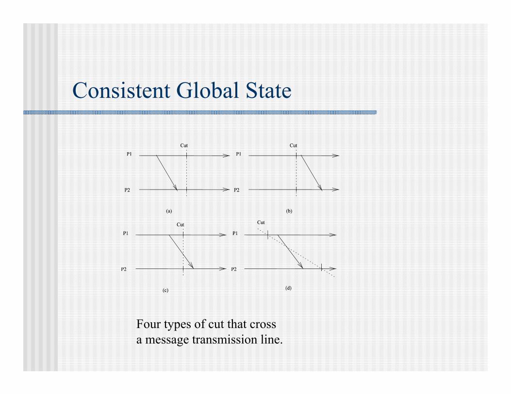
Consistent Global State
Four types of cut that cross a message transmission line.

Consistent Global State (Cont’d.)
A cut is consistent iff no two cut events are causally related. Strongly consistent: no (c) and (d). Consistent: no (d) (orphan message). Inconsistent: with (d).
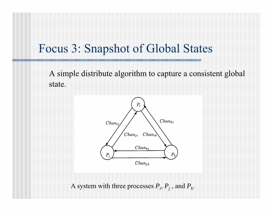
Focus 3: Snapshot of Global States
A simple distribute algorithm to capture a consistent global state.
A system with three processes Pi, Pj , and Pk.

Chandy and Lamport's Solution
Rule for sender P : [ P records its local state ||P sends a marker along all the channels on which a marker has not been
sent. ]

Chandy and Lamport's Solution (Cont’d.)
Rule for receiver Q: /* on receipt of a marker along a channel chan */ [ Q has not recorded its state
[ record the state of chan as an empty sequence and follow the "Rule for sender"
] Q has recorded its state
[ record the state of chan as the sequence of messages received along chan after the latest state recording but before receiving the marker
] ]

Chandy and Lamport's Solution (Cont’d.)
It can be applied in any system with FIFO channels (but with variable communication delays).
The initiator for each process becomes the parent of the process, forming a spanning tree for result collection.
It can be applied when more than one process initiates the process at the same time.

Focus 4: Lamport's Logical Clocks
Based on a “happen-before” relation that defines a partial order on events
Rule1. Before producing an event (an external send or internal event), we update LC :
LCi = LCi + d (d > 0) (d can have a different value at each application of Rule1)
Rule2. When it receives the time-stamped message (m, LCj , j), Pi executes the update
LCi = max{Lci, LCj} + d (d > 0)

Focus 4 (Cont’d.)
A total order based on the partial order derived from the happen-before relation
a ( in Pi ) b ( in Pj )iff(1) LC(a) < LC(b) or (2) LC(a) = LC(b) and Pi < Pjwhere < is an arbitrary total ordering of the process set, e.g., <can be defined as Pi < Pj iff i < j.
A total order of events in the table for Example 2:a0 b0 c0 a1 b1 a2 b2 a3 b3 c1 c2 c3

Example 4: Totally-Ordered Multicasting
Two copies of the account at A and B (with balance of $10,000).
Update 1: add $1,000 at A. Update 2: add interests (based on 1% interest rate) at B. Update 1 followed by Update 2: $11,110. Update 2 followed by Update 1: $11,100.

Vector and Matrix Logical Clock
Linear clock: if a b then LCa < LCb
Vector clock: a b iff LCa < LCb
Each Pi is associated with a vector LCi[1..n], where LCi[i] describes the progress of Pi, i.e., its own process. LCi [j] represents Pi’s knowledge of Pj's progress. The LCi[1..n] constitutes Pi’s local view of the logical global time.

Vector and Matrix Logical Clock (Cont’d.)
When d = 1 and init = 0
LCi[i] counts the number of internal events LCi[j] corresponds to the number of events produced by Pj
that causally precede the current event at Pi.

Vector and Matrix Logical Clock (Cont’d.)
Rule1. Before producing an event (an external send or internal event ), we update LCi[i]:
LCi[i] := LCi[i] + d (d > 0)
Rule2. Each message piggybacks the vector clock of the sender at sending time. When receiving a message (m, LCj , j), Pi executes the update.
LCi[k] := max (LCi[k]; LCj[k]), 1 k nLCi[i] := LCi[i] + d

Example 5
An example of vector clocks.

Example 6: Application of Vector Clock
Internet electronic bulletin board service
When receiving m with vector clock LCj from process j, Piinspects timestamp LCj and will postpone delivery until all messages that causally precede m have been received.
Network News.

Matrix Logical Clock
Each Pi is associated with a matrix LCi[1..n, 1..n] where LCi[i, i] is the local logical clock. LCi[k, l] represents the view (or knowledge) Pi has about
Pk's knowledge about the local logical clock of Pl.
Ifmin(LCi[k, i]) t
then Pi knows that every other process knows its progress until its local time t.

Physical Clock
Correct rate condition:i |dPCi(t)/ dt - 1 | <
Clock synchronization condition:i j |PCi(t) - PCj(t)| <

Lamport's Logical Clock Rules for Physical Clock For each i, if Pi does not receive a message at physical time t,
then PCi is differentiable at t and dPC(t)/dt > 0. If Pi sends a message m at physical time t, then m contains
PCi(t). Upon receiving a message (m, PCj) at time t, process Pi sets
PCi to maximum (PCi(t - 0), PCj + m) where m is a predetermined minimum delay to send message m from one process to another process.

Focus 5: Clock Synchronization
UNIX make program: Re-compile when file.c's time is large than file.o's. Problem occurs when source and object files are generated at different
machines with no global agreement on time.
Maximum drift rate : 1- dPC/dt 1+ Two clocks (with opposite drift rate ) may be 2t apart at a time
after last synchronization. Clocks must be resynchronized at least every /2 seconds in order to
guarantee that they will be differ by no more than .

Cristian's Algorithm
Each machine sends a request every /2 seconds. Time server returns its current time PCUTC (UTC: Universal
Coordinate Time). Each machines changes its clock (normally set forward or
slow down its rate). Delay estimation: (Tr - Ts - I)/2, where Tr is receive time, Ts
send time, and I interrupt handling time.

Cristian's Algorithm (Cont’d.)
Getting correct time from a time server.

Three Ways to Demonstrate the Properties
Testing and debugging (run the program and see what happens)
Operational reasoning (exhaustive case analysis) Assertional reasoning (abstract analysis)

Synchronous vs. Asynchronous Systems
Synchronous Distributed Systems:
The time to each step of a process (program) has known bounds.
Each message will be received within a known bound. Each process has a local clock whose drift rate from real time
has a known bound.

Distributed Algorithms: Traversal
Tarry’s algorithm:
A process forwards the token through the same channel once. A process forwards the token to its parent only when there is no other option.
Complexity: 2E messages and at most 2E time units.

Distributed Algorithms: Traversal (cont’d)
Depth-first search algorithm:
Whenever possible, the token is forwarded to a process that did not hold the token yet; otherwise, it is sent back to its parent.
Complexity: same as Tarry’s algorithm

Distributed Algorithms: Traversal (cont’d)
Extensions to avoid visited nodes:
Include the IDs of visited nodesComplexity: 2(N-1) in time and in messages, but O(N log N) in bit complexity
Awerbuch’s extension: the first-time process with the token informs its neighborsComplexity: 4N-2 in time and 4E in messages
Cidon’s extension: improves on Awerbuch’s extensionComplexity: 2(N-1) in time and 4E in messages

Distributed Algorithms: Echo
Echo algorithm Initiator starts by sending a token to all its neighbors. When a node receives a token for the first time, it makes the sender its
parent, and sends the token to all its neighbors. When a node has received messages from all its neighbors, it sends a
message to its parent. When the initiator has received messages from all its neighbors, it stops.
General wave algorithm A process often needs to gather information from all other processes. Usually the process starts with an initiator and ends with the same imitator
(after collecting all data/results from all other processes). When the wave algorithm is issued at multiple nodes. Many waves, except
one, will fail (as some processes refuse to participate)

Distributed Algorithms: Termination
Dijkstra-Scholten (tree-based): The initiator of the root of the tree. Upon receiving a message:
If the receiving process is currently not in the tree: the process joins the tree by becoming a child of the sender.
If the receiving process is already in the computation: the process immediately sends an acknowledgment message to the sender.
When a process has no more children and has become idle, the process detaches itself from the tree by sending an acknowledgment to its tree parent.
Termination occurs when the initiator has no children and has become idle.
Example: global snapshot (with one king)

Distributed Algorithms: Termination (cont’d)
Shavit-Francez (forest-based): Same as Dijkstra-Scholten, except with multiple initiators. Each non-initiator joining one tree. Termination detection initiated by multiple initiators through a wave algorithmExample: global snapshot (with multiple kings)
Other termination algorithms: Weight-throwing algorithm: dividing a fixed weight over the active processes Rana’s algorithm: waves tagged with logical clocks Safra’s algorithm: token-based traversal

Other Algorithms: Parallel Algorithms
PRAM model Parallel random access memory EREW, ERCW, CREW, CRCW models Chap. 2 of JaJa’s
“an introduction to parallel algorithms”
BSP model by L. Valiant (1990) Bulk synchronous parallel (BSP) Sequential composition of “supersteps”
Local computation Process communication Barrier synchronization
Virtual Processors
LocalComputation
GlobalCommunication
Barrier Synchronization

Parallel Algorithm: Bitonic sorter by K. Batcher
Sorting network based on Bitonic sequence Up-then-Down or Down-then-Up O(n log2(n)) comparators O(log2(n)) latency
Also Batcher’s odd-even sort

Barrier: dissemination barrier
Processes p0, p1, …, pN-1, n starts from 0 until log2N -1 Notifies process p(i+2
n) mod N,
Waits for notification by process P(i-2n) mod N, and
Processes to round n+1

Exercise 21.Consider a system where processes can be dynamically created or
terminated. A process can generate a new process. For example, P1generates both P2 and P3. Modify the happened-before relation and the linear logical clock scheme for events in such a dynamic set of processes.
2. For the distributed system shown in the figure below.

Exercise 2 (Cont’d)
Provide all the pairs of events that are related. Provide logical time for all the events using
linear time, and vector time Assume that each LCi is initialized to zero and d = 1.
3. Provide linear logical clocks for all the events in the system given in Problem 2. Assume that all LC's are initialized to zero and the d's for Pa, Pb, and Pc are 1, 2, 3, respectively. Does condition a b LC(a) < LC(b) still hold? For any other set of d's? and why?

Table of Contents Introduction and Motivation Theoretical Foundations Distributed Programming Languages Distributed Operating Systems Distributed Communication Distributed Data Management Reliability Applications Conclusions Appendix

Three Issues
Use of multiple PEs Cooperation among the PEs Potential for survival to partial failure

Control Mechanisms
Four basic sequential control mechanisms withtheir parallel counterparts.
Statement type \Control type
Sequential control Parallel Control
Sequential/parallel statement
Begin S1, S2
endParbegin S1, S2
ParendFork/join
Alternative statement goto, case if C thenS1 else S2
Guarded commands: G C
Repetitive statement for … do doall, for all
Subprogram procedureSubroutine
proceduresubroutine

Focus 6: Expressing Parallelism
A precedence graph of eight statements.
parbegin/parend statementS1;[[S2;[S3||S4];S5;S6]||S7];S8

Focus 6 (Cont’d.)
fork/join statements1;c1:= 2;fork L1; s2; c2:=2; fork L2;s4; go to L3;
L1: s3; L2: join c1;
s5; L3: join c2;
s6;
A precedence graph.

Dijkstra's Semaphore + Parbegin/ParendS(i): A sequence of P operations; Si; a sequence of Voperations
s: a binary semaphore initialized to 0.
S(1): S1;V(s12);V(s13) S(2): P(s12);S2;V(s24);V(s25) S(3): P(s13);S3;V(s35) S(4): P(s24);S4;V(s46) S(5): P(s25);P(s35);S5;V(s56) S(6): P (s46); P (s56); S6

Focus 7: Concurrent Execution
R(Si), the read set for Si, is the set of all variables whose values are referenced in Si.
W(Si), the write set for Si, is the set of all variables whose values are changed in Si.
Bernstein conditions: R(S1) W(S2) = W(S1) R(S2) = W(S1) W(S2) =

Example 7
S1 : a := x + y, S2 : b := x z, S3 : c := y - 1, and S4 : x := y + z. S1||S2, S1||S3, S2||S3, and S3||S4.
Then, S1||S2||S3 forms a largest complete subgraph.

Example 7 (Cont’d.)
A graph model for Bernstein's conditions.

Alternative statement in DCDL (CSP like distributed control description language)
[ G1 C1 G2 C2 … Gn Cn ].
Alternative Statement

Calculate m = max{x, y}:[x y m := x y x m := y]
Example 8

Repetitive Statement
*[ G1 C1 G2 C2 … Gn Cn ].

Example 9
meeting-time-scheduling ::= t := 0;
*[ t := a(t) t := b(t) t := c(t) ]

Communication and Synchronization
One-way communication: send and receive Two -way communication: RPC(Sun), RMI(Java and
CORBA), and rendezvous (Ada) Several design decisions:
One-to one or one-to-many Synchronous or asynchronous One-way or two-way communication Direct or indirect communication Automatic or explicit buffering Implicit or explicit receiving

Primitives Example Languages
PARALLELISMExpressing parallelism
ProcessesObjectsStatementsExpressionsClauses
MappingStaticDynamicMigration
Ada, Concurrent C, Lina, NIL Emerald, Concurrent SmalltalkOccamPar Alfl, FX-87Concurrent PROLOG, PARLOG
Occam, Star ModConcurrent PROLOG, ParAlflEmerald
COMMUNICATIONMessage Passing
Point-to-point messagesRendezvousRemote procedure callOne-to-many messages
Data SharingDistributed data StructuresShared logical variables
NondeterminismSelect statementGuarded Horn clauses
CSP, Occam, NILAda, Concurrent CDP, Concurrent CLU, LYNXBSP, StarMod
Lina, OrcaConcurrent PROLOG, PARLOG
CSP, Occam, Ada, Concurrent C, SRConcurrent PROLOG, PARLOG
PARTIAL FILURESFailure detectionAtomic transactionsNIL
Ada, SRArgus, Aeolus, Avalon

Message-Passing Library for Cluster Machines (e.g., Beowulf clusters)
Parallel Virtual Machine (PVM):www.epm.ornl/pvm/pvm_home.html
Message Passing Interface (MPI):www.mpi.nd.edu/lam/www-unix.mcs.anl.gov/mpi/mpich/
Java multithread programming:www.mcs.drexel.edu/~shartley/ConcProjJava www.ora.com/catalog/jenut
Beowulf clusters:www.beowulf.org

Message-Passing (Cont’d.)
Asynchronous point-to-point message passing: send message list to destination receive message list {from source}
Synchronous point-to-point message passing: send message list to destination receive empty signal from destination receive message list from sender send empty signal to sender

Example 10
The squash program replaces every pair of consecutive asterisks "**" by an upward arrow “”.
input::= * [ send c to squash ]output::= * [ receive c from squash ]

Example 10 (Cont’d.)
squash::=*[ receive c from input
[ c * send c to output [ c = * receive c from input;
[ c * send * to output;send c to output
c = * send to output ]
] ]
]

Focus 8: Fibonacci Numbers
F(i) = F(i-1) + F (i - 2) for i > 1, with initial values F(0) = 0 and F(1) = 1.
F(i) = ( i -’i )/( -’) ,where = (1+50.5)/2 (golden ratio) and ’ = (1-50.5)/2.
0, 1, 2, 3, 5, 8, 13, 21, 35, 54, …

Focus 8 (Cont’d.)
A solution for F (n).

Focus 8 (Cont’d.)
f(0) ::= send n to f(1);receive p from f(2); receive q from f(1); ans := q
f(-1) ::= receive p from f(1)

Focus 8 (Cont’d.)
f(i) ::= receive n from f(i - 1);[ n > 1 [ send n - 1 to f(i + 1);
receive p from f(i + 2);receive q from f(i + 1);send p + q to f(i - 1);send p + q to f(i - 2) ]
n = 1 [ send 1 to f(i - 1);send 1 to f(i - 2) ]
n = 0 [ send 0 to f(i - 1);send 0 to f(i - 2) ]
]
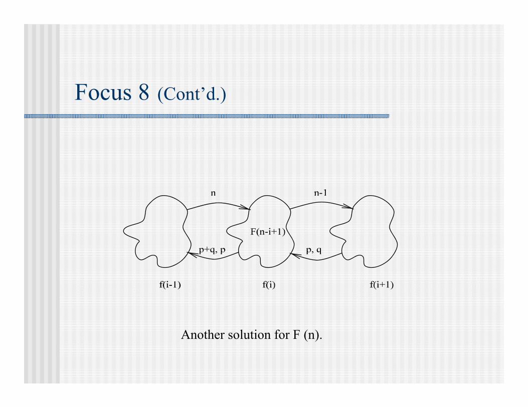
Another solution for F (n).
Focus 8 (Cont’d.)

f(0)::= [ n > 1 [ send n to f(1);
receive p from f(1); receive q from f(1); ans := p]
n = 1 ans := 1 n = 0 ans := 0
]
Focus 8 (Cont’d.)

f(i)::= receive n from f(i - 1);[ n > 1 [ send n - 1 to f(i + 1);
receive p from f(i + 1);receive q from f(i + 1);send p + q to f(i - 1);send p to f(i - 1)]
n = 1 [ send 1 to f(i - 1);send 0 to f(i - 1)
] ]
Focus 8 (Cont’d.)

Focus 9: Message-Passing Primitives of MPI
MPI_Isend: asynchronous communication MPI_send: receipt-based synchronous communication MPI_ssend: delivery-based synchronous communication MPI_sendrecv: response-based synchronous communication

Focus 9 (Cont’d.)
Message-passing primitives of MPI: Isend, send, ssend, sendrecv.

Focus 10: Interprocess Communication in UNIX
Socket: int socket (int domain, int type, int protocol). domain: normally internet. type: datagram or stream. protocol: TCP (Transport Control Protocol) or UDP (User Datagram
Protocol)
Socket address: an Internet address and a local port number.
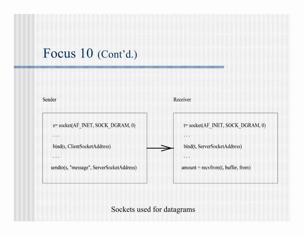
Focus 10 (Cont’d.)
Sockets used for datagrams

High-Level (Middleware) Communication Services
Achieve access transparency in distributed systems Remote procedure call (RPC) Remote method invocation (RMI)

Remote Procedure Call (RPC)
Allow programs to call procedures located on other machines. Traditional (synchronous) RPC and asynchronous RPC.
RPC.

Remove Method Invocation (RMI)
RMI.

Robustness
Exception handling in high level languages (Ada and PL/1)
Four Types of Communication Faults A message transmitted from a node does not reach its
intended destinations Messages are not received in the same order as they were
sent A message gets corrupted during its transmission A message gets replicated during its transmission

If a remote procedure call terminates abnormally (the time out expires) there are four possibilities. The receiver did not receive the call message. The reply message did not reach the sender. The receiver crashed during the call execution and either
has remained crashed or is not resuming the execution after crash recovery.
The receiver is still executing the call, in which case the execution could interfere with subsequent activities of the client.
Failures in RPC

Exercise 3
1.(The Welfare Crook by W. Feijen) Suppose we have three long magnetic tapes each containing a list of names in alphabetical order. The first list contains the names of people working at IBM Yorktown, the second the names of students at Columbia University and the third the names of all people on welfare in New York City. All three lists are endless so no upper bounds are given. It is known that at least one person is on all three lists. Write a program to locate the first such person (the one with the alphabetically smallest name). Your solution should use three processes, one for each tape.

Exercise 3 (Cont’d.)
2.Convert the following DCDL expression to a precedence graph.
[ S1 || [ [ S2 || S3 ]; S4 ] ]
Use fork and join to express this expression.
3.Convert the following program to a precedence graph:
S1;[[S2;S3||S4;S5||S6]||S7];S8

Exercise 3 (Cont’d.)
4.G is a sequence of integers defined by the recurrence Gi = Gi-1+ Gi-3 for i > 1, with initial values G0 = 0, G1 = 1, and G2 = 1. Provide a DCDL implementation of Gi and use one process for each Gi.
5.Using DCDL to write a program that replaces a*b by a band a**b by a b, where a and b are any characters other than *. For example, if a1a2*a3**a4***a5 is the input string then a1a2 a3 a4***a5 will be the output string.

Table of Contents Introduction and Motivation Theoretical Foundations Distributed Programming Languages Distributed Operating Systems Distributed Communication Distributed Data Management Reliability Applications Conclusions Appendix

Distributed Operating Systems
Operating Systems: provide problem-oriented abstractions of the underlying physical resources.
Files (rather than disk blocks) and sockets (rather than raw network access).

Selected Issues Mutual exclusion and election
Non-token-based vs. token-based Election and bidding
Detection and resolution of deadlock Four conditions for deadlock: mutual exclusion, hold and wait, no
preemption, and circular wait. Graph-theoretic model: wait-for graph Two situations: AND model (process deadlock) and OR model
(communication deadlock)
Task scheduling and load balancing Static scheduling vs. dynamic scheduling

Mutual Exclusion and Election
Requirements: Freedom from deadlock. Freedom from starvation. Fairness.
Measurements: Number of messages per request. Synchronization delay. Response time.
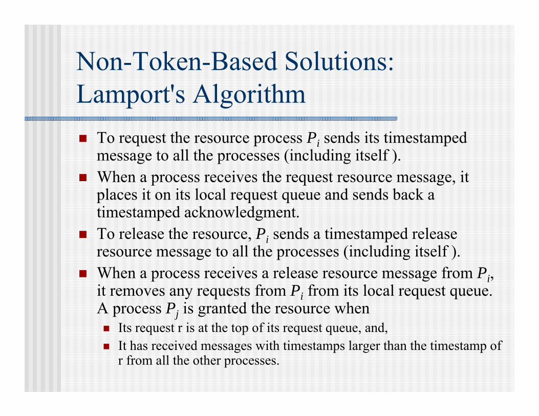
Non-Token-Based Solutions: Lamport's Algorithm To request the resource process Pi sends its timestamped
message to all the processes (including itself ). When a process receives the request resource message, it
places it on its local request queue and sends back a timestamped acknowledgment.
To release the resource, Pi sends a timestamped release resource message to all the processes (including itself ).
When a process receives a release resource message from Pi, it removes any requests from Pi from its local request queue. A process Pj is granted the resource when Its request r is at the top of its request queue, and, It has received messages with timestamps larger than the timestamp of
r from all the other processes.

Example for Lamport’s Algorithm

Extension
There is no need to send an acknowledgement when process Pj receives a request from process Pi after it has sent its own request with a timestamp larger than the one of Pi's request.
An example for Extended Lamport’s Algorithm

Ricart and Agrawala's Algorithm
It merges acknowledge and release messages into one message reply.
An example using Ricart and Agrawala's algorithm.

Token-Based Solutions: Ricart and Agrawala's Second Algorithm
When token holder Pi exits CS, it searches other processes in the order i + 1,i + 2,…,n,1,2,…,i - 1 for the first j such that the timestamp of Pj 's last request for the token is larger than the value recorded in the token for the timestamp of Pj 's last holding of the token.

Token-based Solutions (Cont’d)
Ricart and Agrawala's second algorithm.

P(i)::=*[ request-resourceconsume release-resource treat-request-message others ]
distributed-mutual-exclusion ::= ||P(i:1..n)
clock: 0,1,…, (initialized to 0) token-present: Boolean (F for all except one process)token-held: Boolean (F) token: array (1..n) of clock (initialized 0) request: array (1..n) of clock (initialized 0)
Pseudo Code

others::= all the other actions that do not request to enter the critical section.
consume::= consumes the resource after entering the critical section
request-resource::=[ token present = F [ send (request-signal, clock, i) to all;
receive (access-signal, token); token-present:= T; token-held:= T
]]
Pseudo Code (Cont’d)
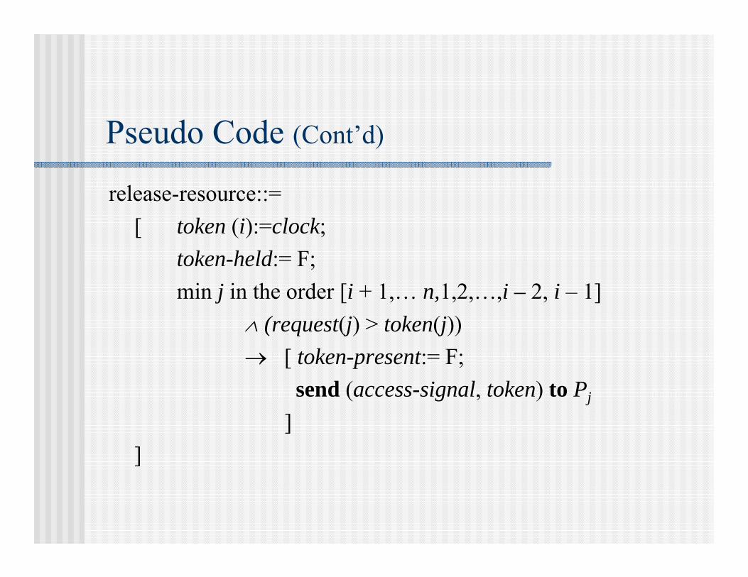
release-resource::=[ token (i):=clock;
token-held:= F;min j in the order [i + 1,… n,1,2,…,i – 2, i – 1]
(request(j) > token(j)) [ token-present:= F;
send (access-signal, token) to Pj
]]
Pseudo Code (Cont’d)

treat-request-message::=[ receive (request-signal, clock; j)
[request(j):=max(request(j),clock);token-present token-held release-resource
] ]
Pseudo Code (Cont’d)
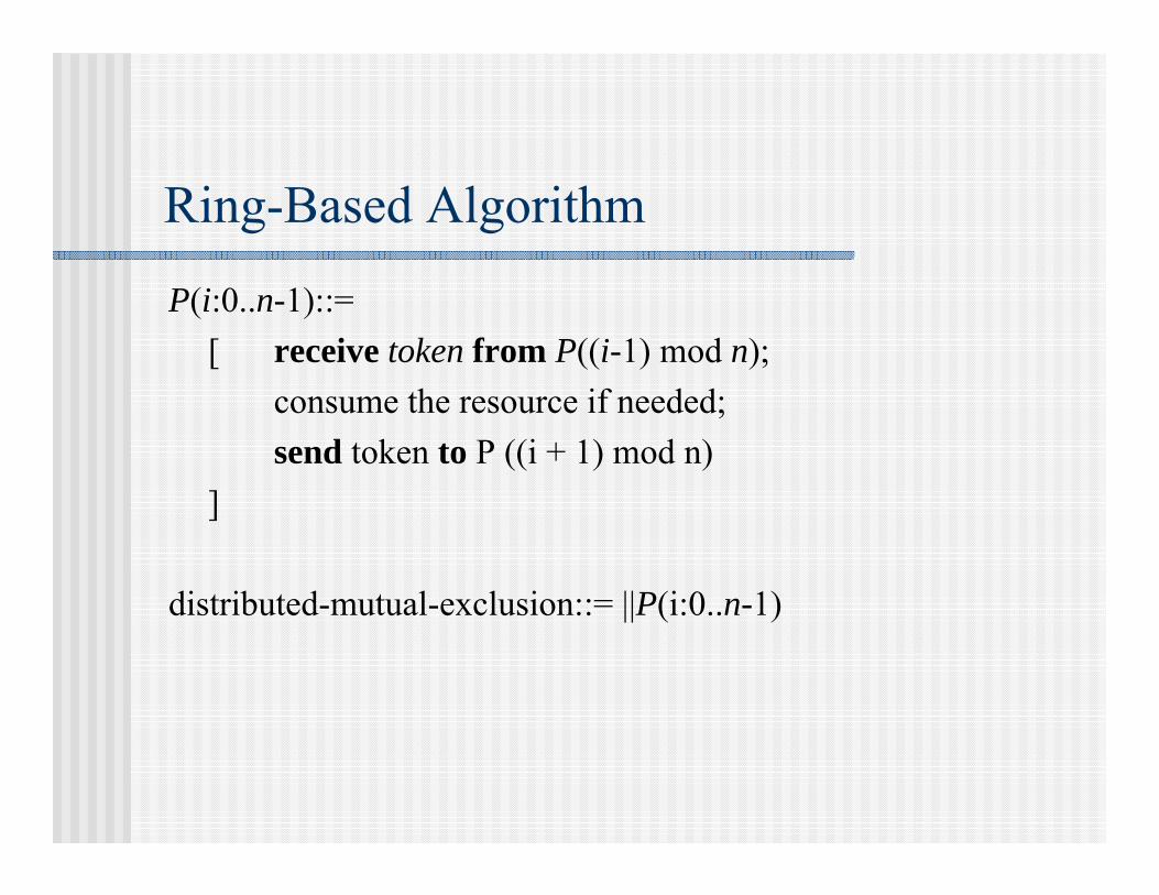
Ring-Based Algorithm
P(i:0..n-1)::=[ receive token from P((i-1) mod n);
consume the resource if needed; send token to P ((i + 1) mod n)
]
distributed-mutual-exclusion::= ||P(i:0..n-1)
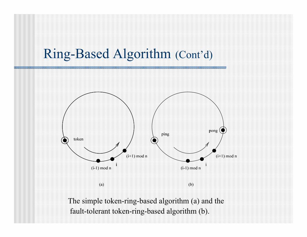
Ring-Based Algorithm (Cont’d)
The simple token-ring-based algorithm (a) and thefault-tolerant token-ring-based algorithm (b).

Tree-Based Algorithm
A tree-based mutual exclusion algorithm.

Maekawa's Algorithm
Permission from every other process but only from a subset of processes.
If Ri and Rj are the request sets for processes Pi and Pj , then Ri Rj .

Example 11
R1 : {P1; P3; P4} R2 : {P2; P4; P5} R3 : {P3; P5; P6} R4 : {P4; P6; P7} R5 : {P5; P7; P1} R6 : {P6; P1; P2} R7 : {P7; P2; P3}

Related Issues
Election: After a failure occurs in a distributed system, it is often necessary to reorganize the active nodes so that they can continue to perform a useful task.
Bidding: Each competitor selects a bid value out of a given set and sends its bid to every other competitor in the system. Every competitor recognizes the same winner.
Self-stabilization: A system is self-stabilizing if, regardless of its initial state, it is guaranteed to arrive at a legitimate state in a finite number of steps.

Focus 11: Chang and Robert’s algorithm
Election on a ring Election and elected signals Smallest ID is the winner Two rounds of circulation O(n log n) messages

Garcia-Molina's Bully Algorithm for Election
When P detects the failure of the coordinator or receives an ELECTION packet, it sends an ELECTION packet to all processes with higher priorities.
If no one responds (with packet ACK), P wins the election and broadcast the ELECTED packet to all.
If one of the higher processes responds, it takes over. P's job is done.
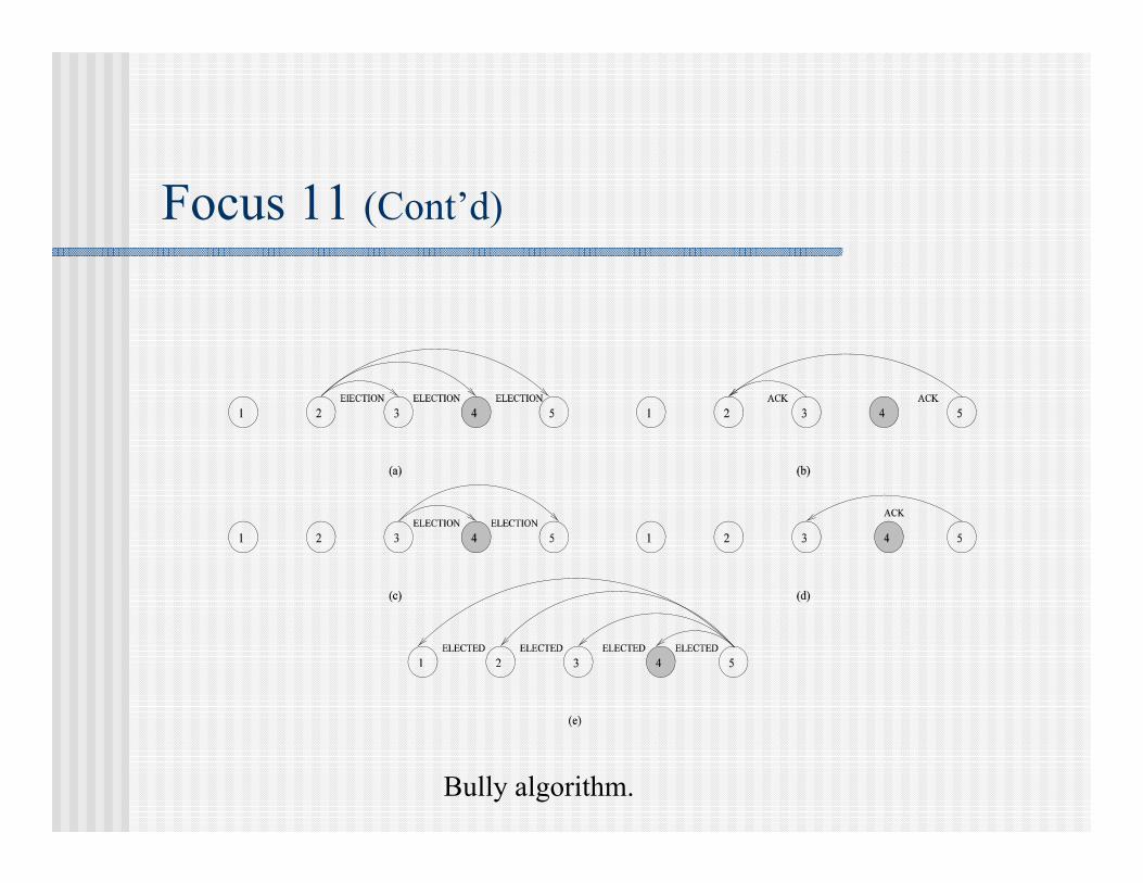
Focus 11 (Cont’d)
Bully algorithm.

Lynch's Non-Comparison-Based Election Algorithms
Process id is tied to time in terms of rounds. Time-slice algorithm: (n, the total number of
processes, is known) Process Pi (with its id(i)) sends its id in round id(i)2n, i.e., at most one
process sends its id in every 2n consecutive rounds. Once an id returns to its original sender, that sender is elected. It sends
a signal around the ring to inform other processes of its winning status.
message complexity: O(n) time complexity: min{id(i)} n

Variable-speed algorithm: (n is unknown) When a process Pi sends its id (id(i)), this id travels at
the rate of one transmission for every 2id(i) rounds. If an id returns to its original sender, that sender is
elected.
message complexity: n + n/2 + n/22 + … + n/2(n-1)
< 2n = O(n) time complexity: 2 min{id(i)}n
Lynch's Algorithms (Cont’d)

Dijkstra's Self-Stabilization
Legitimate state P : A system is in a legitimate state P if and only if one process has a privilege.
Convergence: Starting from an arbitrary global state, S is guaranteed to reach a global state satisfying P within a finite number of state transitions.

Example 12
A ring of finite-state machines with three states. A privileged process is the one that can perform state transition.
For Pi, 0 < i n - 1, PiPi-1 Pi := Pi-1, P0=Pn-1 P0:=(P0+1) mod k
Theorem: If k > n, then Dijkstra’s token ring for mutual exclusion always eventually reaches a correct configuration.
For n > 2, theorem also hold if k = n-1.

Table 1: Dijkstra’s self-stabilization algorithm (n =3 and k =4).
P0 P1 P2 Privileged processes
Process to make move
2 1 2 P0,P1,P2 P0
3 1 2 P1,P2 P1
3 3 2 P2 P2
3 3 3 P0 P0
0 3 3 P1 P1
0 0 3 P2 P2
0 0 0 P0 P0
1 0 0 P1 P1
1 1 0 P2 P2
1 1 1 P0 P0
2 1 1 P1 P1
2 2 1 P2 P2
2 2 2 P0 P0
3 2 2 P1 P1
3 3 2 P2 P2
3 3 3 P0 P0

Non-Convergence ExampleWhen n > 3, k = n-2.
Infinite computation exists in which always n-1 processes are privileged

Extensions
The role of demon (that selects one privileged process) The role of asymmetry. The role of topology. The role of the number of states

Detection and Resolution of Deadlock
Mutual exclusion. No resource can be shared by more than one process at a time.
Hold and wait. There must exist a process that is holding at least one resource and is waiting to acquire additional resources that are currently being held by other processes.
No preemption. A resource cannot be preempted. Circular wait. There is a cycle in the wait-for graph.

Detection and Resolution of Deadlock (Cont’d)
Two cities connected by (a) one bridge and by (b) two bridges.

Strategies for Handling Deadlocks
Deadlock prevention Deadlock avoidance (based on "safe state") Deadlock detection and recovery Different Models
AND condition OR condition

Types of Deadlock
Resource deadlock Communication deadlock
An example of communication deadlock

Conditions for Deadlock
AND model: a cycle in the wait-for graph. OR model: a knot in the wait-for graph.

Conditions for Deadlock (Cont’d)
A knot (K) consists of a set of nodes such that for every node a in K , all nodes in K and only the nodes in K are reachable from node a.
Two systems under the OR condition with (a) no deadlock and without (b) deadlock.

Focus 12: Rosenkrantz' Dynamic Priority Scheme (using timestamps)
T1:lock A;lock B;transaction starts;unlock A; unlock B;
wait-die (non-preemptive method)[ LCi < LCj halt Pi (wait)
LCi LCj kill Pi (die) ]
wound-wait (preemptive method)[ LCi < LCj kill Pj (wound)
LCi LCj halt Pi (wait)]

Example 13
A system consisting of five processes.
Process id Priority 1st request time Length Retry interval
P1 2 1 1 1
P2 1 1.5 2 1
P3 4 2.1 2 2
P4 5 3.3 1 1P5 3 4.0 2 3

Example 13 (Cont’d)
wound-wait:
wait-die:

Load Distribution
A taxonomy of load distribution algorithms.

Static Load Distribution (task scheduling)
Processor interconnections Task partition
Horizontal or vertical partitioning. Communication delay minimization partition. Task duplication.
Task allocation

Models
Task precedence graph: each link defines the precedence order among tasks.
Task interaction graph: each link defines task interactions between two tasks.
(a) Task precedence graph and (b) task interaction graph.

Example 14
Mapping a task interaction graph (a) to a processor graph (b).

Example 14 (Cont’d)
The dilation of an edge of Gt is defined as the length of the path in Gp onto which an edge of Gt is mapped. The dilation of the embedding is the maximum edge dilation of Gt.
The expansion of the embedding is the ratio of the number of nodes in Gt to the number of nodes in Gp.
The congestion of the embedding is the maximum number of paths containing an edge in Gp where every path represents an edge in Gt.
The load of an embedding is the maximum number of processes of Gt assigned to any processor of Gt.

Periodic Tasks With Real-time Constraints
Task Ti has request period ti and run time ci. Each task has to be completed before its next request. All tasks are independent without communication.

Liu and Layland's Solutions (priority-driven and preemptive)
Rate monotonic scheduling (fixed priority assignment). Tasks with higher request rates will have higher priorities.
Deadline driven scheduling (dynamic priority assignment). A task will be assigned the highest priority if the deadline of its current request is the nearest.

Schedulability Deadline driven schedule: iff
n
ci/ti 1i=0
Rate monotonic schedule: ifn
ci/ti n(21/n - 1);i=0
may or may be not when n
n(21/n - 1) < ci/ti 1i=0

Example 15 (schedulable)
T1: c1 = 3, t1 = 5 and T2: c2 = 2, t2 = 7 (with the same initial request time).
The overall utilization is 0:887 > 0:828 (bound for n = 2).
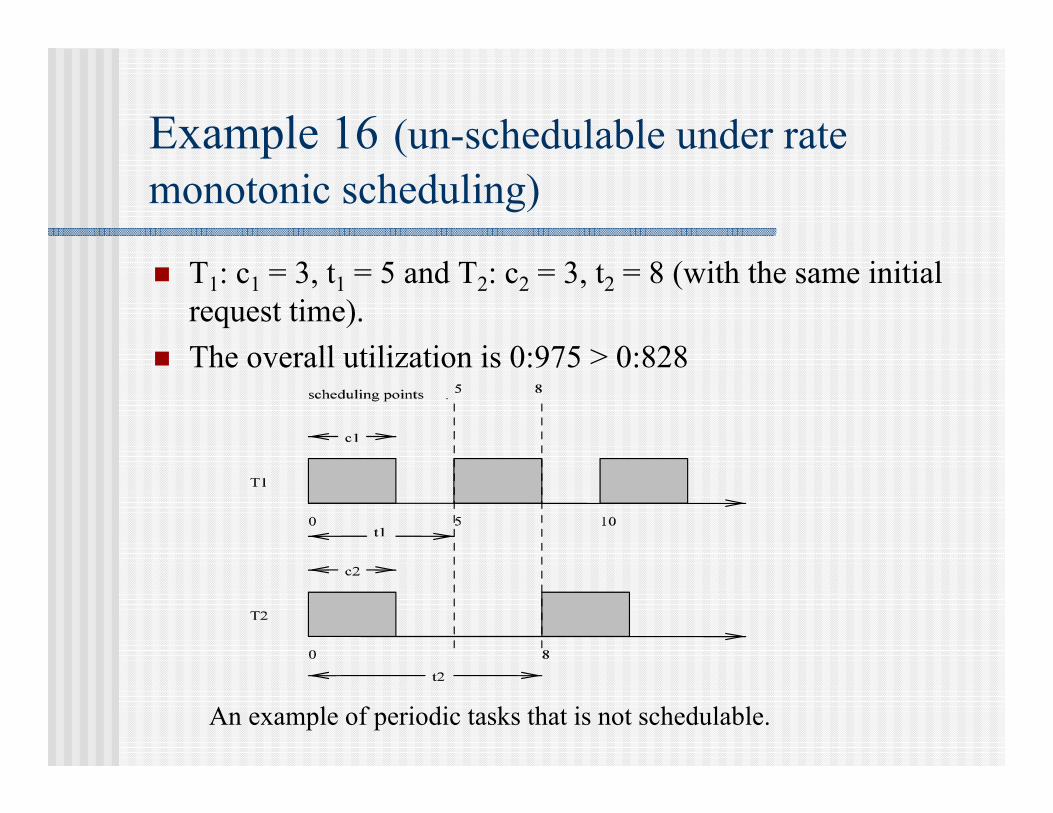
Example 16 (un-schedulable under rate monotonic scheduling)
T1: c1 = 3, t1 = 5 and T2: c2 = 3, t2 = 8 (with the same initial request time).
The overall utilization is 0:975 > 0:828
An example of periodic tasks that is not schedulable.

Example 16 (Cont’d)
If each task meets its first deadline when all tasks are started at the same time then the deadlines for all tasks will always be met for any combination of starting times.
scheduling points for task T : T 's first deadline and the ends of periods of higher priority tasks prior to T 's first deadline.
If the task set is schedulable for one of scheduling points of the lowest priority task, the task set is schedulable; otherwise, the task set is not schedulable.

Example 17 (schedulable under rate monotonic schedule)
c1 = 40, t1 = 100, c2 = 50, t2 = 150, and c3 = 80, t3 = 350. The overall utilization is 0:2 + 0:333 + 0:229 = 0:762 < 0:779
(the bound for n > 3). c1 is doubled to 40. The overall utilization is
0:4+0:333+0:229 = 0:962 > 0:779. The scheduling points for T3: 350 (for T3), 300 (for T1 and
T2), 200 (for T1), 150 (for T2), 100 (for T1).

Example 17 (Cont’d)
c1 + c2 + c3 t1,40 + 50 + 80 > 100;2c1 + c2 + c3 t2,80 + 50 + 80 > 150;2c1 + 2c2 + c3 2t1,80 + 100 + 80 > 200;3c1 + 2c2 + c3 2t2,120 + 100 + 80 = 300;4c1 + 3c2 + c3 t3,160 + 150 + 80 > 350.

Example 17 (Cont’d)
A schedulable periodic task.

Dynamic Load Distribution (load balancing)
A state-space traversal example.

Dynamic Load Distribution (Cont’d)
A dynamic load distribution algorithm has six policies: Initiation Transfer Selection Profitability Location Information

Focus 13: Initiation
Sender-initiated approach:
Sender-initiated load balancing.

Focus 13 (Cont’d)
/* a new task arrives */queue length HWM
* [ poll_set := ;
[| poll_set | < poll_limit [ select a new node u randomly;
poll_set := poll_set node u; queue_length at u < HWM
transfer a task to node u and stop]
]]
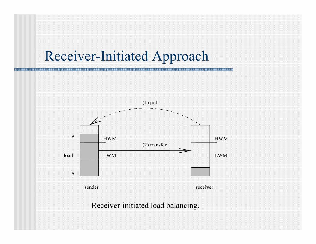
Receiver-Initiated Approach
Receiver-initiated load balancing.

Receiver-Initiated Approach (Cont’d)
/* a task departs */ queue length < LWM [ poll limit:= ;
* [ | poll_set | < poll limit [ select a new node u randomly;poll_set := poll set node u;queue_length at u > HWM
transfer a task from node u and stop]
] ]

Bidding Approach
Bidding algorithm.

Focus 14: Sample Nearest Neighbor Algorithms
Diffusion At round t + 1 each node u exchanges its load Lu(t) with its neighbors'
Lv(t). Lu(t + 1) should also include new incoming load u(t) between rounds
t and t + 1. Load at time t + 1:
Lu(t + 1) = Lu(t) + u,v(Lv(t)- Lu(t)) + u(t)v A(u)
where 0 u,v 1 is called the diffusion parameter of nodes u and v.

Gradient
Maintain a contour of the gradients formed by the differences in load in the system.
Load in high points (overloaded nodes) of the contour will flow to the lower regions (underloaded nodes) following the gradients.
The propagated pressure of a processor u, p(u), is defined as p(u) = 0 (if u is lightly loaded) 1 + min{p(v)|v A(u)} (otherwise)

Gradient (Cont’d)
(a) A 4 x 4 mesh with loads. (b) The corresponding propagated pressure of each node (a node is lightly loaded if its load is less than 3).

Dimension Exchange: Hypercubes
A sweep of dimensions (rounds) in the n-cube is applied. In the ith round neighboring nodes along the ith dimension
compare and exchange their loads.

Dimension Exchange: Hypercubes (Cont’d)
Load balancing on a healthy 3-cube.

Extended Dimension Exchange: Edge-Coloring
Extended dimension exchange model through edge-coloring.

Exercise 4
1. Apply wound-wait and wait-die schemes to the example shown in Table 2.2. Show the state transition sequence for the following system with n = 3 and
k = 5 using Dijkstra's self-stabilizing algorithm. Assume that P0 = 3, P1 = 1, and P2 = 4.
3. Determine if there is a deadlock in each of the following wait-for graphs assuming the OR model is used.

Exercise 4 (Cont’d)
Table 2: A system consisting of four processes.
Process id Priority 1st request time Length Retry interval
Resource(s)
P1 3 1 1 1 A
P2 4 1.5 2 1 B
P3 1 2.5 2 2 A,B
P4 2 3 1 1 B,A
4. Consider the following two periodic tasks (with the same request time)
Task T1: c1 = 4, t1 = 9
Task T2: c2 = 6, t2 = 14
(a) Determine the total utilization of these two tasks and compare it with Liu and Layland's least upper bound for the fixed priority schedule. What conclusion can you derive?

Exercise 4 (Cont’d)
(b) Show that these two tasks are schedulable using the rate-monotonic priority assignment. You are required to provide such a schedule.
(c) Determine the schedulability of these two tasks if task T2 has a higher priority than task T1 in the fixed priority schedule.
(d) Split task T2 into two parts of 3 units computation each and show that these two tasks are schedulable using the rate-monotonic priority assignment.
(e) Provide a schedule (from time unit 0 to time unit 30) based on deadline driven scheduling algorithm. Assume that the smallest preemptive element is one unit.

Exercise 4 (Cont’d)
5. For the following 4 x 4 mesh find the corresponding propagated pressure of each node. Assume that a node is considered lightly loaded if its load is less than 2.

Table of Contents Introduction and Motivation Theoretical Foundations Distributed Programming Languages Distributed Operating Systems Distributed Communication Distributed Data Management Reliability Applications Conclusions Appendix

Distributed Communication
One-to-all (broadcast)
Different types of communication
One-to-one (unicast)
One-to-many (multicast)

Classification
Special purpose vs. general purpose. Minimal vs. nonminimal. Deterministic vs. adaptive. Source routing vs. distributed routing. Fault-tolerant vs. non fault-tolerant. Redundant vs. non redundant. Deadlock-free vs. non deadlock-free.

A general PE with a separate router.
Router Architecture

Topology. The topology of a network, typically modeled as a graph, defines how PEs are connected.
Routing. Routing determines the path selected to forward a message to its destination(s).
Flow control. A network consists of channels and buffers. Flow control decides the allocation of these resources as a message travels along a path.
Switching. Switching is the actual mechanism that decides how a message travels from an input channel to an output channel: store-and-forward and cut-through (wormhole routing).
Four Factors for Communication Delay

General-Purpose Routing
Source routing: link state (Dijkstra's algorithm)
A sample source routing

General-Purpose Routing (Cont’d)
Distributed routing: distance vector (Bellman-Ford algorithm)
A sample distributed routing

Distributed Bellman-Ford Routing Algorithm
Initialization. With node d being the destination node, set D(d) = 0 and label all other nodes (., ).
Shortest-distance labeling of all nodes. For each node v d do the following: Update D(v) using the current value D(w) for each neighboring node w to calculate D(w) + l(w, v) and perform the following update:
D(v) := min{D(v), D(w) + l(w; v)}

Distributed Bellman-Ford Algorithm(Cont’d)

Example 18
A sample network.

Example 18 (Cont’d)
Bellman-Ford algorithm applied to the network with P5 being the destination.
Round P1 P2 P3 P4
Initial (., ) (., ) (., ) (., )
1 (., ) (., ) (5,20) (5,2)
2 (3,25) (4,3) (4,4) (5,2)3 (2,7) (4,3) (4,4) (5,2)

Looping Problem
Time next node
0 1 2 3 K, 4<k<15 16 17 18 19 (20, )
P2 7 7 9 9 2n/2 +7 23 23 25 25 27
P3 9 9 11 11 2n/2+9 25 25 25 25 25*
Time next node
0 1 2 3 K, 4<k<15
16 17 18 19 (20, )
P1 11 11 13 13 2n/2 +9 25 27 27 29 29
P3 7 7 9 9 2n/2 +7 23 23 23 23 23
P3 3 5 5 7 2n/2+3 19 21 21 23* 23
(a) Network delay table of P1
(b) Network delay table of P2
Link (P4; P5) fails at the destination P5.

Time next node
0 1 2 3 K, 4<k<15 16 17 18 19 (20, )
P1 12 12 12 14 2n/2 +10 26 28 28 30 30
P2 6 6 8 8 2n/2 +5 22 22 24 24 26
P4 4 6 6 8 2n/2 +4 20 22 22 24 24
P5 20 20 20 20 20 20 20* 20 20 20
Time next node
0 1 2 3 K, 4<k<15
16 17 18 19 (20, )
P2 4 4 6 6 2n/2 +4 20 20 22 22 24
P3 6 6 8 8 2n/2 +5 22 22 22 22 22*
P5
(c) Network delay table of P3
(d) Network delay table of P4
Looping Problem (Cont’d)

Special-Purpose Routing
E-cube routing in n-cube: u w as a navigation vector.
A routing in a 3-cube with source 000 and destination 110: (a)Single path. (b) Three node-disjoint paths.

Binomial-Tree-Based Broadcasting in N-Cubes
The construction of binomial trees.

Hamiltonian-Cycle-Based Broadcasting in N-Cubes
(a) A broadcasting initiated from 000 with coordinated sequence (CS): {3, 2, 1}.
(b) A Hamiltonian cycle in a 3-cube.
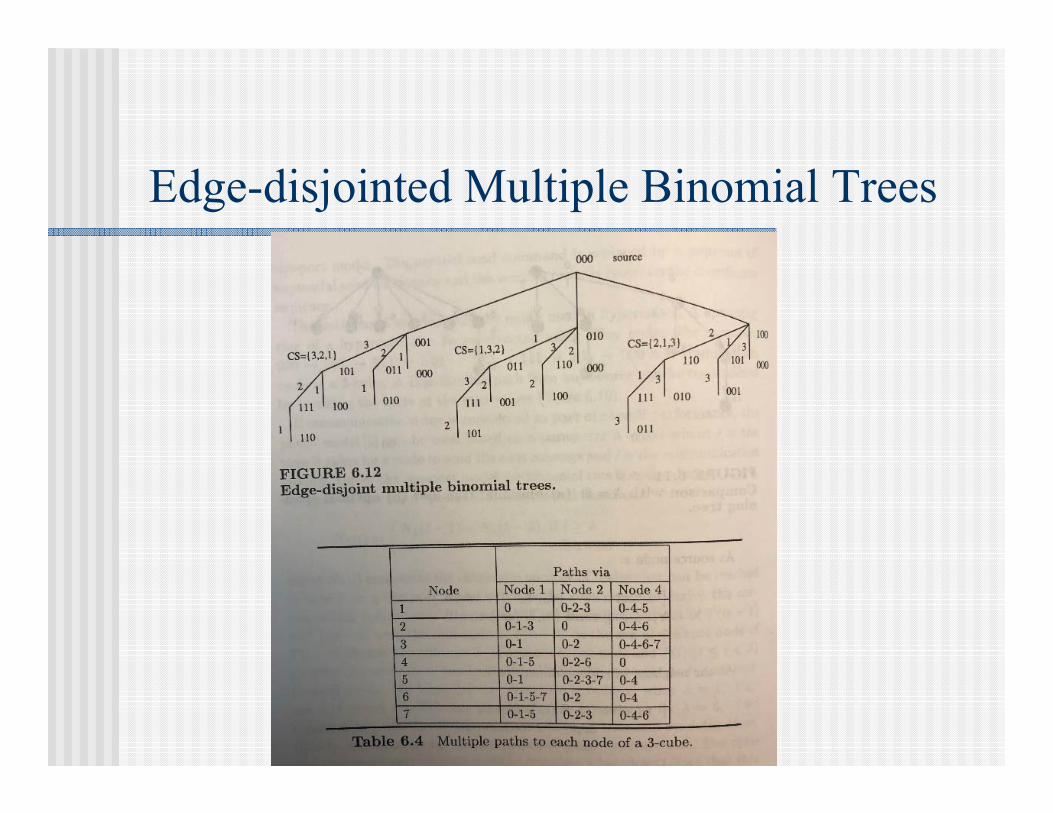
Edge-disjointed Multiple Binomial Trees

Cut-through: recursive doubling
(L) one-port and (R) all-port on ring One-port on mesh with minimum total distance using eyes: (a) 2x2, (b) 4x4, and (c) 2k x 2k meshes

Parameterized Communication Model
Postal model: = l/s, where l is the communication latency and s is the
latnecy for a node to send the next message. Under the one-port model the binomial tree is optimal when
= 1.
N (t) = N (t-1) + N (t- ), if t ≥ ; 1, otherwise

Example 19: Broadcast Tree
Comparison with = 6: (a) binomial tree and (b) optimal spanning tree.

Multicasting
Multicast path Minimum spanning tree (for a graph) Shortest path tree (for a graph) Steiner tree (without a graph): a minimum tree
that includes all destinations.
Three-points Steiner treewith the Fermat point S
(e.g., all angles ≤ 120o )

Focus 15: Fault-Tolerant Routing
Wu's safety level: The safety level associated with a node is an approximated measure of the
number of faulty nodes in the neighborhood. Initially all faulty nodes have 0 as safety levels and all non-faulty nodes
have n. Let (S0,S1,S2,…,Sn-1), 0 Si n, be the non-descending safety status
sequence of node a's neighboring nodes in an n-cube. Iteratively do the following: If (S0,S1,S2,…,Sn-1) (0,1,2,…,n-1) then S(a)
= n else if (S0,S1,S2,…Sk-1) (0,1,2,…,k-1) ^ (Sk = k-1) then S(a) = k.
Insight: Embedding of Bn in terms of Bn-1, Bn-2, …, B1, and B0 in any orientation.

Focus 15: Fault-Tolerant Routing (Cont’d)
Distributed algorithms: iterative exchanges (maximum n rounds) with neighbors’ safety levels
A node a is called safe if its level is n, i.e., S(a) =n

Fault-Tolerant Routing (Cont’d)
If the safety level of a node is k, there is at least one Hamming distance path from this node to any node within k-hop.If there are at most n faults, every unsafe node has a safe neighbor.
A fault-tolerant routing using safety levels.

Fault-Tolerant Broadcasting
If the source node is n-safe, there exists an n-level injured spanning binomial tree in an n-cube: source can reach all non-faulty nodes through a Hamming distance path.
Broadcasting in a faulty 4-cube.

Wu's Extended Safety Level in 2-D Meshes
A sample region of minimal paths.

Safety BlockSafety block: (1) All faulty nodes are unsafe. All nonfaulty nodes are initially safe.
(2) If a nonfaulty node has two or more faculty/unsafe neighbors, it is unsafe.Extended safety block: (1). (2) …has a faulty/unsafe neighbor in both dimensions…Wu’s orthogonal convex region: All safe nodes are enabled. A unsafe node is
initially disabled, but it is changed to the enabled status if it has two or more enabled neighbors.
(L) Regular and (R) extended safe/unsafe Enabled/disabled for (L) regular and (R) for extended

Deadlock-Free Routing
Virtual channels and virtual networks:
(a) A ring with two virtual channels, (b) channel dependency graph of (a), and (c) two virtual rings vr1 and vr0.

Focus 16: Deadlock-Free Routing Without Virtual Channels
XY-routing in 2-D meshes: X dimension followed by Y dimension.
Glass and Ni's Turn model: Certain turns are forbidden.
(a) Abstract cycles in 2-d meshes, (b) four turns (solid arrows) allowed in XY-routing, (c) six turns allowed in positive-first routing, and (d) six turns allowed in negative-first routing.

Planar-Adaptive Routing
For general k-ary n-cubes, select n+1 2-D planes A0, A1, …, An. Ai spans dimension di and di+1.
Three virtual channels are used: one for di and two for di+1: di,2, di+1,0, and di+1, 1. (Second subscript is virtual channel number.)
Each plane has one positive and one negative subnetworks.
Positive and negativeNetworks in di and di+1

Escape channels
Regular channels: non-waiting Escape channels: waiting
Strongly connected requirement Strictly decreasing path requirement: for any pair of nodes, a
decreasing (labelled) path exist.
Theorem: The minimum number of channels needed to meet the above two conditions is 2n-1, where n is the number of nodes.
L. Sheng and J. Wu, “A Note on “A Tight Lower Bound on the Number of Channels Required for Deadlock-Free Wormhole Routing.

Exercise 51. Provide an addressing scheme for the following extended mesh (EM)
which is a regular 2-D mesh with additional diagonal links. Provide a general shortest routing algorithm for EMs.
2. Repeat Example 18 after changing (P1, P3) to 4 and (P3, P5) to 12.
3. Suppose the postal model is used for broadcasting and = 8. What is the maximum number of nodes that can be reached in time unit 10. Derive the corresponding broadcast tree.

Exercise 5 (Cont’d)
4. Consider the following turn models: West-first routing. Route a message first west, if necessary, and then
adaptively south, east, and north. North-last routing. First adaptively route a message south, east, and west;
route the message north last. Negative-first routing. First adaptively route a message along the negative X
or Y axis; that is, south or west, then adaptively route the message along the positive X or Y axis.
(a) Show all the turns allowed in each of the above three routings.(b) Show the corresponding routing paths using (1) positive-first, (2) west-first, (3) north-last, and (4) negative-first routing for the following unicasting: (2,1) to (5,9), (7,1) to (5,3), (6,4) to (3,1), and (1,7) to (5,2).
5. Wu and Fernandez (1992) gave the following safe and unsafe node definition: A nonfaulty node is unsafe if and only if either of the following conditions is true: (a) There are two faulty neighbors, or (b) there are at least three unsafe or faulty neighbors. Consider a 4-cube with faulty nodes 0100, 0011, 0101, 1110, and 1111. Find out the safety status (safe or unsafe) of each node

Exercise 5 (Cont’d)
Repeat the above using Wu’s safety vector. Critically compare safety node, safety level, and safety vector in terms of fault-tolerance capability and complexity. (J. Wu, Reliable communication in cube-based multipcomputersusing safety vectors, IEEE TPDS, 9, (4), April 1998, 321-334.)
6. To support fault-tolerant routing in 2-D meshes, D. J. Wang (1999) proposed the following new model of faulty block: Suppose the destination is in the first quadrant of the source. Initially, label all faulty nodes as faulty and all non-faulty nodes as fault-free. If node u is fault-free, but its north neighbor and east neighbor are faulty or useless, u is labeled useless. If node u is fault-free, but its south neighbor and west neighbor are faulty or can't-reach, u is labeled can't-reach. The nodes are recursively labeled until there are no new useless or can't-reach nodes.
(a) Give an intuitive explanation of useless and can't-reach. (b) Re-write the definition when the destination is in the second quadrant of the source.

Exercise 5 (Cont’d)
7. Chiu proposed an odd-even turn model, which is an extension to Glass and Ni's turn model. The odd-even turn model tries to prevent the formation of the rightmost column segment of a cycle. Two rules for turn are given in: Rule 1: Any packet is not allowed to take an EN (east-north) turn at
any nodes located in an even column, and it is not allowed to take an NW turn at any nodes located in an odd column.
Rule 2: Any packet is not allowed to take an ES turn at any nodes located in an even column, and it is not allowed to take a SW turn at any nodes located in an odd column.
(a) Use your own word to explain that the odd-even turn model is deadlock-free.
(b) Show all the shortest paths (permissible under the extended odd-even turn model) for
(a) s1:(0, 0) and d1:(2,2) and (b) s2:(0,0) and d2:(3,2)(c) Prove Properties 1, 2, and 3 of Wu and Li's marking process for ad hoc
wireless networks.

Table of Contents Introduction and Motivation Theoretical Foundations Distributed Programming Languages Distributed Operating Systems Distributed Communication Distributed Data Management Reliability Applications Conclusions Appendix

Distributed Data Management
Data objects Files Directories
Data objects are dispersed and replicated Unreplicated Fully replicated Partially replicated

Serializability Theory
Atomic execution A transaction is an "all or nothing" operation. The concurrent execution of several transactions affects the
database as if executed serially in some order. The interleaved order of the actions of a set of concurrent transactions is called a schedule.

Example 22: Concurrent Transactions
T1 begin1 read A (obtaining A_balance) 2 read B (obtaining B_balance)3 write A_balance-$10 to A4 write B_balance+$10 to Bend
T2 begin1 read B (obtaining B balance)2 write B_balance-$5 to Bend

Three types of conflict: r-w (read-write), w-r (write-read), and w-w (write-write).
rj[x] reads from wi[x] iff wi[x] < rj[x]. There is no wk[x] such that wi[x] < wk[x] < rj[x].
Two schedules are equivalent iff Every read operation reads from the same write operation in both
schedules. Both schedules have the same final writes.
When a non-serial schedule is equivalent to a serial schedule, it is called serializable schedule.
Concepts
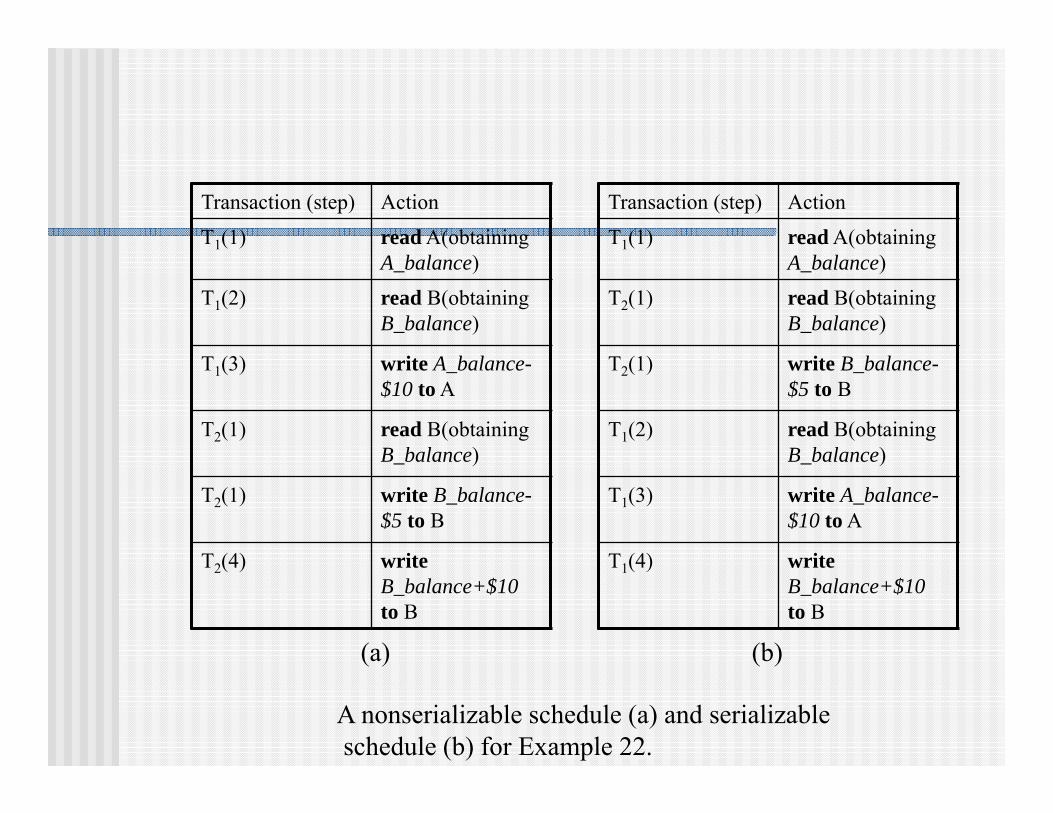
A nonserializable schedule (a) and serializableschedule (b) for Example 22.
Transaction (step) Action
T1(1) read A(obtaining A_balance)
T1(2) read B(obtaining B_balance)
T1(3) write A_balance-$10 to A
T2(1) read B(obtaining B_balance)
T2(1) write B_balance-$5 to B
T2(4) writeB_balance+$10to B
(a)
Transaction (step) Action
T1(1) read A(obtaining A_balance)
T2(1) read B(obtaining B_balance)
T2(1) write B_balance-$5 to B
T1(2) read B(obtaining B_balance)
T1(3) write A_balance-$10 to A
T1(4) writeB_balance+$10to B
(b)

Concurrency Control
Locking scheme Timestamp-based scheme Optimistic concurrency control

Focus 18: Two-Phase Locking
A transaction is well-formed if it locks an object before accessing it, does not lock an object that is already locked, and before it completes, unlocks each object it has locked.
A schedule is two-phase if no object is unlocked before all needed objects are locked.
Two-phase locking

Example 23: Well-Formed, Two-Phase Transactions
T1: beginlock A read A (obtaining A balance) lock B read B (obtaining B balance) write A_balance-$10 to A unlock A write B_balance+$10 to B unlock Bend
T2: beginlock B read B (obtaining B balance) write B_balance-$5 to B unlock B end

Different Looking Schemes Centralized locking algorithm: distributed
transactions, but centralized lock management. Primary-site locking algorithm: each object has a
single site designated as its primary site (as in INGRES).
Decentralized locking: The lock management duty is shared by all the sites.

Focus 19: Timestamp-based Concurrency Control
Timer(x) (Timew(x)): the largest timestamp of any read (write) processed thus far for object x. (Read) If ts < Timew(x) then the read request is rejected
and the corresponding transaction is aborted; otherwise, it is executed and Timer(x) is set to max{Timer(x), ts}.
(Write) If ts < Timew(x) or ts < Timer(x), then the write request is rejected; otherwise, it is executed and Timew(x) is set to ts.

Example 24
Timer(x) = 4 and Timew(x) = 6 initially. Sample:
read(x,5), write(x,7), read(x,9), read(x, 8), write(x,8) First and last are rejected and Timer(x) = 7, Timew(x)
= 9 when completed.

Conservative Timestamp Ordering
Each site keeps a write queue (W-queue) and a read queue (R-queue). A read (x, ts) request is executed if all W-queues are
nonempty and the first write on each queue has a timestamp greater than ts; otherwise, the read request is buffered in the R-queue.
A write (x, ts) request is executed if all R-queues and W–queues are nonempty and the first read (write) on each R-queue (W-queue) has a timestamp greater than ts; otherwise, the write request is buffered in the W-queue.

Strict Consistency
Any read returns the result of the most recent write. Impossible to enforce, unless
All writes are instantaneously visible to all processes. All reads get the then-current values, no matter how
quickly next writes are done. An absolute global time order is maintained.

Weak Consistency
Sequential consistency: All processes see all shared accesses in the same order.
Causal consistency: All processes see causually-related shared accesses in the same order.
FIFO consistency: All process see writes from each process in the order they were issued.
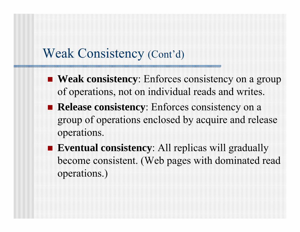
Weak consistency: Enforces consistency on a group of operations, not on individual reads and writes.
Release consistency: Enforces consistency on a group of operations enclosed by acquire and release operations.
Eventual consistency: All replicas will gradually become consistent. (Web pages with dominated read operations.)
Weak Consistency (Cont’d)
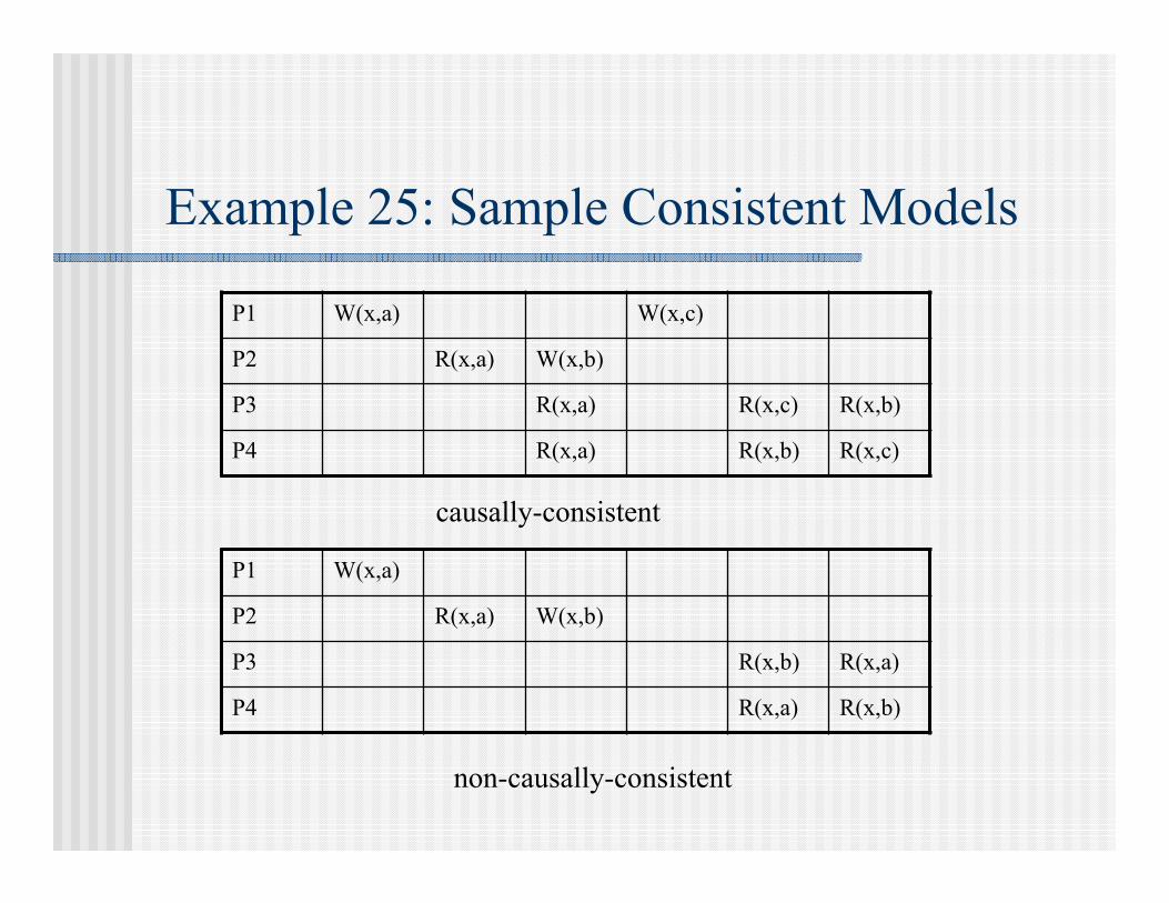
Example 25: Sample Consistent Models
causally-consistent
P1 W(x,a) W(x,c)
P2 R(x,a) W(x,b)
P3 R(x,a) R(x,c) R(x,b)
P4 R(x,a) R(x,b) R(x,c)
P1 W(x,a)
P2 R(x,a) W(x,b)
P3 R(x,b) R(x,a)
P4 R(x,a) R(x,b)
non-causally-consistent

Example 25: Sample Consistent Models
Linearizable: sequentially-consistent, but taking ordering based on synchronized clocks
sequentially-consistent
P1 W(x,a)
P2 W(x,b)
P3 R(x,b) R(x,a)
P4 R(x, b) R(x,a)
P1 W(x,a)
P2 W(x,b)
P3 R(x, b) R(x,a)
P4 R(x, a) R(x,b)
non-sequentially-consistent

Example 25 (Cont’d)
FIFO-consistent
P1 W(x,a)
P2 R(x,a) W(x,b) W(x,c)
P3 R(x,b) R(x,a) R(x,c)
P4 R(x,a) R(x,b) R(x,c)

Update Propagation for Multiple Copies State versus Operations
Propagate a notification of an update (such as invalidate signal) Propagate data Propagate the update operation
Pull versus Push Push-based approach (server-based) Pull-based approach (client-based) Lease-based approach (hybrid of push and pull)
Consistency of duplicated data Write-invalidate vs. write-through Quorum-voting as an extension of single-write/multiple-read

Focus 20: Quorum-Voting
w > v/2 and r + w > v
where w and r are write and read quorum and v is the total number of votes.

Hierarchical Quorum Voting
A 3-level tree in the hierarchical quorum voting with read quorum= 2 and write quorum = 3.

Jim Gray's Two-Phase Commitment Protocol
The finite state machine model for the two-phase commit protocol.

Phase 1At the coordinator:
/*prec: initiate state (q) */ 1. The coordinator sends a commit_request message to every participantand waits for replies from all the participants.
/*postc: waiting state (w) */
At participants:
/*prec: initiate state (q)*/ 1. On receiving the commit_request message, a participant takes the
following actions. If the transaction executing at the participant is successful, it writes undo and redo log, and sends a yes message to the coordinator; otherwise, it sends a no message.
/*postc: wait state (w) if yes or abort state (a) if no*/

Phase 2At the coordinator
/*prec: wait state (w)*/1. If all the participants reply yes then the coordinator writes a commit record
into the log and then sends a commit message to all the participants. Otherwise, the coordinator sends an abort message to all the participants.
/*postc: commit state (c) if commit or abort state (a) if abort */
2. If all the acknowledgments are received within a timeout period, the coordinator writes a complete record to the log; otherwise, it resends the commit/abort message to those participants from which no acknowledgments were received.

Phase 2 (Cont’d)
At the participants
/*prec: wait state (w) */ 1. On receiving a commit message, a participant releases all the resources and
locks held for executing the transaction and sends an acknowledgment.
/*postc: commit state (c) *//*prec: abort state (a) or wait state (w) */
2. On receiving an abort message, a participant undoes the transaction using the undo log record, releases all the resources and locks held by it, and sends an acknowledgment.
/*postc: abort state (a) */
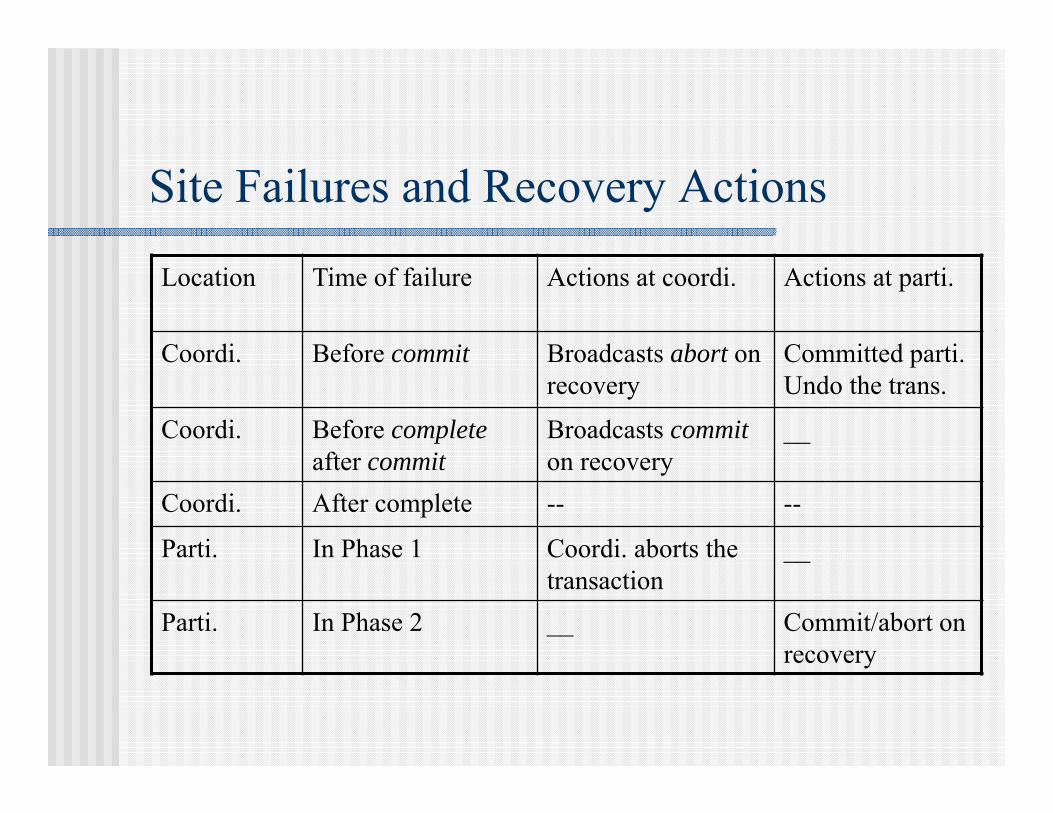
Site Failures and Recovery Actions
Location Time of failure Actions at coordi. Actions at parti.
Coordi. Before commit Broadcasts abort on recovery
Committed parti. Undo the trans.
Coordi. Before complete after commit
Broadcasts commit on recovery
__
Coordi. After complete -- --
Parti. In Phase 1 Coordi. aborts the transaction
__
Parti. In Phase 2 __ Commit/abort on recovery

Two Types of Logs
undo log allows an uncommitted transaction to record in stable storage values it wrote. (T1, T4, and T5 in the example)
redo log allows a transaction to commit before all the values written have been recorded in stable storage. (T2 and T7)
A recovery example.

A protocol is synchronous within one state transition if one site never leads another site by more than one state transition.
concurrent set C(s): the set of all states of every site that may be concurrent with state s.
In two-phase commitment: C (w(c)) = {c(p), a(p), w(p)} and C (q(p)) = {q(c), w(c)} (w(c) is the w state of coordinator and q(p) is the q state of participant).
In three-phase commitment: C (w(c)) = {q(p), w(p), a(p)} and C (w(p)) = {a(c), p(c), w(c)}.
Concepts

Skeen's Three-Phase Commitment Protocol

Exercise 61. For the following two transactions:
T1 begin1 read A (obtaining A balance) 2 write A balance- $10 to A 3 read B (obtaining B balance)4 write B balance+$10 to B
end
T2 begin1 read A (obtaining A balance)2 write A balance+$5 to Aend
(a) Provide all the interleaved executions (or schedules). (b) Find all the serializable schedules among the schedules obtained in (a).

Exercise 6 (Cont’d)
2. Point out serializable schedules in the following
L1 = w2(y)w1(y)r3(y)r1(y)w2(x)r3(x)r3(z)r2(z) L2 = r3(z)r3(x)w2(x)r2(z)w1(y)r3(y)w2(y)r1(y) L3 = r3(z)w2(y)w2(x)r1(y)r3(y)r2(z)r3(x)w1(y) L4 = r2(z)w2(y)w2(x)w1(y)r1(y)r3(y)r3(z)r3(x)
3. A voting method called voting-with-witness replaces some of the replicas by witnesses. Witnesses are copies that contain only the version number but no data. The witnesses are assigned votes and will cast them when they receive voting requests. Although the witnesses do not maintain data, they can testify to the validity of the value provided by some other replica. How should a witness react when it receives a read quorum request? What about a write quorum request? Discuss the pros and cons of this method.

Table of Contents Introduction and Motivation Theoretical Foundations Distributed Programming Languages Distributed Operating Systems Distributed Communication Distributed Data Management Reliability Applications Conclusions Appendix

Type of Faults
Types of faults: Hardware faults Software faults Communication faults Timing faults
Schneider’s classification: Omission failure Failstop failure (detectable) Crash failure (undetectable) Crash and link failure Byzantine failure

Redundancy
Hardware redundancy: extra PE's, I/O's Software redundancy: extra version of software modules Information redundancy: error detecting code Time redundancy: additional time used to perform a
function

Fault Handling Methods
Active replication Passive replication Semi-active replication

Building Blocks of Fault-Tolerant Design
Stable storage is a logical abstraction for a special storage that can survive system failure.
Fail-stop processors do not perform any incorrect action and simply cease to function.
An atomic action is a set of operations which are executed indivisibly by hardware. That is, either operations are completed successfully and fully or the state of the system remains unchanged (operations are not executed at all).

Storage of checkpoints Checkpointing methods
An example of domino effect.
Domino Effect

Focus 21: Byzantine Faults
Several divisions of the Byzantine army camp outside an enemy city. Each division commanded by its own general. Generals from different divisions communicate only through messengers. Some of the generals may be traitors. After observing the enemy, the generals must decide upon a common battle plan.

Two Requirements
All loyal generals decide upon the same plan of action A small number of traitors cannot cause the loyal generals to
adopt a wrong plan
Note Loyal generals may start with different decisions, but end up
the same decision. The final decision must come from at least one loyal
general’s initial decision.

Focus 21 (Cont’d)
Theoretical result Consensus is reachable if n 3m + 1, where n is the total number of
generals and m is the number of traitors.
(m+1)-round of consensus algorithm At the first round, each node, including traitors, broadcasts its initial
decision At the (i+1)th round, each node broadcasts all messages received at ith
round

Agreement Protocol
An algorithm for reaching agreement.
P1* P2 P3 P4First round:(-,v2,v3,v4) (v1
2, -,v3, v4) (v11,v2,- v4) (v1
3,v2, v3,-)Second round:(v1
2, -, v3, v4)(v1
1, v2, -, v4)(v1
3, v2, v3, -)
(v11, v2, -, v4)
(v13, v2, v3, -)
(-, v24, v3
4, v44)
(v11, -, v3, v4)
(v13, v2, v3, -)
(-, v25, v3
5, v45)
(v12, -, v3, v4)
(v11, v2, -, v4)
(-, v26, v3
6, v46)
(d1, d2,d3, d4) (v17, v2, v3, v4) (v1
7, v2, v3, v4) (v17, v2, v3, v4)

No-Agreement Among Three Processes
Cases leading to failure of the Byzantine agreement.

Extended Agreement Protocols Boolean values or arbitrary real values for the decisions. Unauthenticated or authenticated messages. Synchronous or asynchronous. Completely connected network or partially connected
networks. Deterministic or randomized. Byzantine faults or fail-stop faults. Non-totally decentralized control system and, in particular,
hierarchical control systems.

Reliable Communication
Acknowledgement: acknowledge the receipt of each packet. TCP: transport protocol for reliable point-to-point comm. Negative acknowledgement
Signal for a missing packet. Pros: better scalability (without positive acknowledgement). Cons: sender is forced to keep each packet in the buffer forever.

Reliable Group Communication
Feedback suppression: multicast or broadcast each positive (or negative) acknowledge.
Combination of positive and negative acknowledgements

Example 26: Combination of Positive and Negative Acknowledgements in Broadcasting.
Let A be a packet and a (a) the positive (negative) acknowledgement for A.
A,Ba,Cb,Db,Ec,F cd,Cb,Gdef
1.Message A is sent first, acknowledged by the sender of B, which is in turn acknowledged by the senders of C and D.
2. The sender of E acknowledges C and the sender of F acknowledges the receipt of D but a negative acknowledgment of C .
3. Some node (not necessarily the original sender) retransmits C .
4. The sender of G acknowledges both E and F but sends a negative acknowledgment of D (after receiving F ).

Different Types of Reliable Multicasting
Reliable multicast: no message ordering FIFO multicast: FIFO-ordered delivery Causal multicast: causal-ordered delivery Atomic multicast: reliable multicast + total-ordered delivery FIFO atomic multicast: FIFO multicast + total-ordered
delivery Causal atomic multicast: Causal multicast + total-ordered
delivery

Focus 22: Total-Ordered Multicasting
Total-ordered multicasting Each transfer order (message) can be assigned a global sequence
number. There exists a global sequence.
Sequencer The sender sends message to a sequencer The sequencer allocates a global sequence number to the message. The message is delivered by every destination based on the order.

Implementations of Sequencer
Privilege-based (token circulated among the senders) Fixed sequencer (a fixed third party) Moving sequencer(token circulated among the third-party
nodes)

Multicast with Total Order
seq(m1) < seq(m2)
Neither seq(m1) < seq(m2) nor seq(m2) < seq(m1)
Multicast with total order
Multicast without total order

Focus 23: Birman’s Virtual Synchrony Virtual synchrony: reliable multicast with a special property. View: a multicast group. View change: (a) a new process joins, (b) a process leaves,
and(c) a process crashes.
Each view change is multicast to members in the group. Special property: each view change acts as a barrier across
which no multicast can pass. (Application: distributed debugging.)

Focus 23 (Cont’d)
Virtual synchrony.

Implementing a Virtual Synchronous Reliable Multicast
Message received versus message delivered. If message m has been delivered to all members in the group,
m is called stable. Point-to-point communication is reliable (TCP). Sender may crash before completing the multicasting. (Some
members received the message but others did not.)
Message receipt versus message delivery.

At group view Gi, a view changed is multicast. When a process receives the view-change message for Gi+1, it
multicasts to Gi+1 a copy of unstable messages for Gifollowed by a flush message.
A process installs the new view Gi+1 when it has received a flush message from everyone else.
Virtual synchrony.
Implementing a Virtual Synchronous Reliable Multicast (Cont’d)

Reliable ProcessActive model
Passive model

Exercise 71. Use a practical example to illustrate the differences among faults, errors, and failures.
2. Illustrate the correctness of the agreement protocol for authenticated messages using a system of four processes with two faulty processes. You need to consider the following two cases: The sender is healthy and two receivers are faulty (the remaining receiver is healthy). The sender is faulty and one receiver is faulty (the remaining receivers are healthy).
3. In Byzantine agreement protocol k + 1 rounds of message exchanges are needed to tolerant k faults. The number of processes n is at least 3k + 1. Assume P1 and P2 are faulty in a system of n = 7 processes. (a) Show the messages P3 receives in first, second, and third round. (b) Demonstrate the correctness of the protocol by showing the final result
vector (after a majority voting) for P3. (c) Briefly show that result vectors for other non-faulty processes are the
same.

Table of Contents Introduction and Motivation Theoretical Foundations Distributed Programming Languages Distributed Operating Systems Distributed Communication Distributed Data Management Reliability Applications Conclusions Appendix

Distributed Operating Systems
Key issues Communication primitives Naming and protection Resource management Fault tolerance Services: file service, print service, process service, terminal service,
file service, mail service, boot service, gateway service Distributed operating systems vs. network operating
systems Commercial and research prototypes
Wiselow, Galaxy, Amoeba, Clouds, and Mach

Distributed File Systems A file system is a subsystem of an operating system whose
purpose is to provide long-term storage. Main issues:
Merge of file systems Protection Naming and name service Caching Writing policy
Research prototypes: UNIX United, Coda, Andrew (AFS), Frangipani, Sprite, Plan 9,
DCE/DFS, and XFS Commercial:
Amazon S3, Google Cloud Storage, Microsoft Azure, SWIFT (OpenStack)

Distributed Shared Memory
A distributed shared memory is a shared memory abstraction what is implemented on a loosely coupled system.
Distributed shared memory.

Focus 24: Stumm and Zhou's Classification
Central-server algorithm (nonmigrating and nonreplicated). (Client) Sends a data request to the central server. (Central server) Receives the request, performs data
access andsends a response.
(Client) Receives the response.

Focus 24 (Cont’d)
Migration algorithm (migrating and non-replicated). (Client) If the needed data object is not local, determines
thelocation and then sends a request.
(Remote host) Receives the request and then sends the object.
(Client) Receives the response and then accesses the data object (read and /or write).

Focus 24 (Cont’d)
Read-replication algorithm (migrating and replicated)
(Client) If the needed data object is not local, determines the location and sends a request.
(Remote host) Receives the request and then sends the object.

Focus 24 (Cont’d)
(Client) Receives the object and then multicasts by sending either invalidate or update messages to all sites that have a copy of the data object.(Remote host) Receives an invalidation signal and then invalidates its local copy, or receives an update signal and then updates the local copy.(Client) Accesses the data object (write).

Focus 24 (Cont’d)
Full-replication algorithm (non-migrating and replicated) (Client) If it is a write, sends the data object to the
sequencer. (Sequencer) Receives the data object and adds a sequence
number. Sends the client a signal with the sequence number and multicasts the data object together with the sequence number to all the other sites.

Focus 24 (Cont’d)
(Client) Receives the acknowledgment and updates local memory based on the sequence number of each data object.
(Other sites) Receive the data object and update local memory based on the sequence number of each data object.

Focus 24 (Cont’d)
Main Issues: Structure and granularity Coherence semantics Scalability Heterogeneity
Several research prototypes: Dash, Ivy, Munin, and Clouds Alewife (MIT), Treadmarks (Rice), Coherent Virtual machine
(Maryland), and Millipede (Israel Inst. Tech.)

Distributed Database Systems
A distributed database is a collection of multiple, logically interrelated databases distributed over a computer network.
Possible design alternatives: Autonomy Distribution Heterogeneity

Distributed Database Systems (Cont’d)
Alternative architectures.

Essentials of Distributed Database Systems Local autonomy No reliance on a central site Continuous operation Location independence Fragment independence Replication independence Distributed query processing Distributed transaction management Hardware independence Operating system independence Network independence Data independence

Network scaling problem Distributed query processing Integration with distributed operating systems Heterogeneity Concurrency control Security Next-generation database systems:
Object-oriented database management systems Knowledge base management systems
Open Research Problems

Research Prototypes ADDS (Amocha Distributed Database Systems) JDDBS (Japanese Distributed Database Systems) Ingres/star SWIFT (Society for Worldwide Interbank Financial Telecomm) System R, MYRIAD, MULTIBASE, and MERMAID
Commercial products (XML, NewSQL, and NoSQL) Blockchain (popularized by bitcoin) Aerispike, Cassandra, Clusterpoint, Druid (open-source data store) ArangoDB, ClustrixDB, Couchbase, FoundationDB, NueDB, and
OrientDB
Prototypes and Products

Heterogeneous Processing
Tuned use of diverse processing hardware to meet distinct computational needs. Mixed-machine systems. Different execution modes by
inter-connecting several different machine models. Mixed-mode systems. Different execution modes by
reconfigurable parallel architecture obtained by interconnecting the same processors.

Classifications
Single Execution Mode/Single Machine Model (SESM)
Single Execution Mode/Multiple Machine Models (SEMM)
Multiple Execution Modes/Single Machine Model (MESM)
Multiple Execution Modes/Multiple Machine Models (MEMM)

Focus 25: OptimizationAn optimization problem that minimizes
ti,j
such that
cj C
where ti,j equals the time for machine i on code segment j, ciequals the cost for machine i, C equals the specified overall cost constraint.

Table of Contents Introduction and Motivation Theoretical Foundations Distributed Programming Languages Distributed Operating Systems Distributed Communication Distributed Data Management Reliability Applications Conclusions Appendix

"Killer" Applications
Distributed Object-based Systems: CORBA Distributed Document-based Systems: WWW Distributed Coordination-based Systems: JINI Distributed Multimedia Systems: QoS requirements Distributed currency and transactions: Bitcoin and blockchain

Other Applications: MapReduce
A framework for processing highly distributable problems across huge datasets on a file system or a database. Map: In a recursive way, the master node takes the input, divides it
into smaller sub-problems, and distributes them to worker nodes. Reduce: The master node then collects the answers to all the sub-
problems and combines them in some way to form the output. The shuffle is used collect all data through I/O. Usually, shuffle dominates the actual reduce phase.
Apache Hadoop: a software framework that supports data-intensive distributed applications under a free license. It was derived from Google’s MapReduce and Google File System (GFS).
Spark for Big Data and beyond

Pipeline: Map followed by Shuffle
Impact of overlapping map and shuffle
Map pipeline
Shuffle pipeline
WordCount (map-heavy) TeraSort (shuffle-heavy)

Minimize Last Job: Flow Shop
Minimize last job completion time
l-phase flow shop is solvable when l=2 Gm: map-heavy jobs sorted in increasing order of map load Gs: shuffle-heavy jobs sorted in decreasing order of shuffle load
Optimal schedule: Gs followed by Gm
S. M. Johnson, Optimal two-and three-stage production schedules with setup times included, Naval Research Logistics Quarterly, 1954.
Map
ShuffleJ2
J2
J1
J1
J3
J3
J4
J4
J2
J2
J1
J1
J3
J3
J4
J4

Minimize Average Jobs: Strong Pair
Minimize average job completion time, NP-hard in general
Special case one: strong pair J1 and J2 are a strong pair if m1 = s2 and s1 = m2 (m: map, s: shuffle)
Optimal schedule: jobs are strong pairsPair jobs and rank pairs by total workloads
H. Zheng, Z. Wan, and J. Wu, Optimizing MapReduce framework through joint scheduling of overlapping phases, Proc. of IEEE ICCCN, 2016.
Map
ShuffleJ1
J1
J3
J3 J4
J4
J2
J2J1
J1
J3
J3J4
J4
J2
J2

Minimize Average Jobs: Dominant Load
Special case two: when all jobs are map-heavy or shuffle-heavyOptimal schedule:
Sort jobs ascendingly by dominant workload max{m, s}Execute smaller jobs earlier
Map pipeline
Shuffle pipeline
Finishing times J1, J2, J3: 1, 3, 6 vs. J3, J2, J1: 3, 5, 6

Other Applications: Crowdsourcing
How Much Data? Facebook: 40 B photos; 30 B pieces of content shared every month
WeChat: 846 M users and 20 B message per day
Global Internet traffic: quadrupled from 2010 to 2015, reaching 966 EB (1018) per year(All human knowledge created from the dawn of man to 2003 is totaled 5 EB)
640K ought to be enough for anybody.

Big Data Era “In information technology, big data consists of datasets
that grow so large that they become awkward to work with using on-hand database management tools.”
Computers are not efficient in processing or creating certain things: pattern recognition, complex communication, and ideation.
Crowdsourcing: coordinating a crowd (a large group of people online) to do microwork (small jobs) that solves problems (that software or one user cannot easily do)
Crowdsourcing: crowd + outsourcing (through Internet)

The Benefits of Crowdsourcing
Performance Inexpensive and fast The whole is greater than the sum of its parts
Human Processing Unit (HPU) More effective than CPU (for some apps)
• Verification and validation: Image labeling• Interpretation and analysis: language translation• Surveys: Social network survey
High adoption in business (85% of the top global brands) based on eYeka

Basic Components of Crowdsourcing Requester
People submit jobs (microwork) Human Intelligence Tasks (HITs)
Worker People work on jobs
Platform Job management
Amazon Mechanical Turk (MTurk): 18th century chess playing robot with a human inside

Other Applications: PageRank
A link analysis algorithm PR(E): Rage Rank of E likelihood that a person
randomly clicking on links will arrive at any particular page
M(pi): set of pages link to pi, L(pj): the number of outgoing links on pj, d: dumping factor, N: total number of pages.
HITS (Jon Kleinberg): each node has two values in a mutual recursion• Authority: the sum of the Hub
Scores of each node that points to it. • Hub: the sum of the Authority
Scores of each node that it points to.

Other Applications: P2P Systems
Client/server limitations: scalability, single point of failure, etc. P2P: an overlay network no centralized control, e.g., Blockchain Unstructured P2P
Napster: share music, server stores index Gnutella: no server, query flooding Kazza: supernodes to improve scalability Freenet: data caching in reverse path of query BitTorrent: Tit-for-Tat to avoid free-raiders
Structured P2P: distributed hash table (DHT): map key to value Chord: n-node ring, table size: log(n), search time: log(n) CAN: n-node d-dimension mesh, table size: d, search time: d n1/d
Others based on different graphs: De Brujin, Butterfly, and Kautz graphs

P2P Systems: Search
Unstructured P2P BFS and variations (e.g. expanding rings and directed BFS) Probabilistic search and variations (e.g., random walk) Indices-based search and variations (e.g., dominating-set and Bloom filter)
Structured P2P: Chord (hypercube) and CAN (2-D mesh)

Emerging Systems
Wireless networks and mobile computing: mobile agents Move the computation to the data rather than the data to the
computations.
Grid TeraGrid: 13.6 teraflops of Linux Cluster computing power
distributed at the four TeraGrid sites. Open Grid Services Architecture (OGSA): delivering tighter
integration between grid computing networks and Web services technologies.
Grid Computing (via OGSA) as the basis of evolution of Internet computing in the future.

Distributed GridOptIPuter (UC San Diego and U. of Chicago) Parallel optical networks using IP Supernetworks: networks faster than the computers attached to them Parallelism takes the form of multiple wavelengths, or lambdas (1-10
Gbps) A new resource abstraction: distributed virtual computer
E-Science (UK Research Councils, 2001) Large-scale science carried out through distributed global
collaboration enabled by networks, requiring access to very large data collaborations, very large-scale computing resources, and high-performance visualization.

Cloud (edge, fog) ComputingSharing of resources to achieve
coherence and economies of scale similar to utility (e.g. electricity grid) over a network (e.g. Internet)
Characteristics• Agility, API, cost, device,
virtualization, multi-tenancy, reliability, scalability, performance, security, maintenance
Service• Infrastructure as a Service (LaaS)• Platform as a Service (PaaS)• Software as a Service (SaaS)