Embed Size (px)
Citation preview
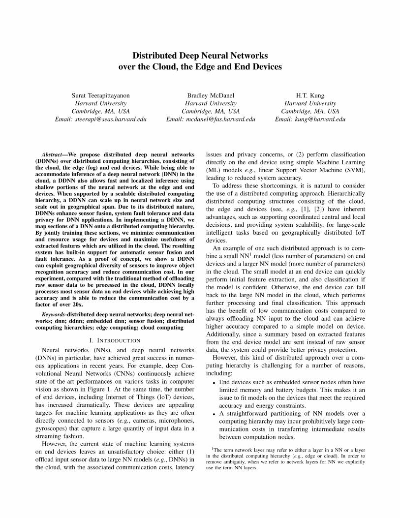
Distributed Deep Neural Networksover the Cloud, the Edge and End Devices
Surat TeerapittayanonHarvard University
Cambridge, MA, USAEmail: [email protected]
Bradley McDanelHarvard University
Cambridge, MA, USAEmail: [email protected]
H.T. KungHarvard University
Cambridge, MA, USAEmail: [email protected]
Abstract—We propose distributed deep neural networks(DDNNs) over distributed computing hierarchies, consisting ofthe cloud, the edge (fog) and end devices. While being able toaccommodate inference of a deep neural network (DNN) in thecloud, a DDNN also allows fast and localized inference usingshallow portions of the neural network at the edge and enddevices. When supported by a scalable distributed computinghierarchy, a DDNN can scale up in neural network size andscale out in geographical span. Due to its distributed nature,DDNNs enhance sensor fusion, system fault tolerance and dataprivacy for DNN applications. In implementing a DDNN, wemap sections of a DNN onto a distributed computing hierarchy.By jointly training these sections, we minimize communicationand resource usage for devices and maximize usefulness ofextracted features which are utilized in the cloud. The resultingsystem has built-in support for automatic sensor fusion andfault tolerance. As a proof of concept, we show a DDNNcan exploit geographical diversity of sensors to improve objectrecognition accuracy and reduce communication cost. In ourexperiment, compared with the traditional method of offloadingraw sensor data to be processed in the cloud, DDNN locallyprocesses most sensor data on end devices while achieving highaccuracy and is able to reduce the communication cost by afactor of over 20x.
Keywords-distributed deep neural networks; deep neural net-works; dnn; ddnn; embedded dnn; sensor fusion; distributedcomputing hierarchies; edge computing; cloud computing
I. INTRODUCTION
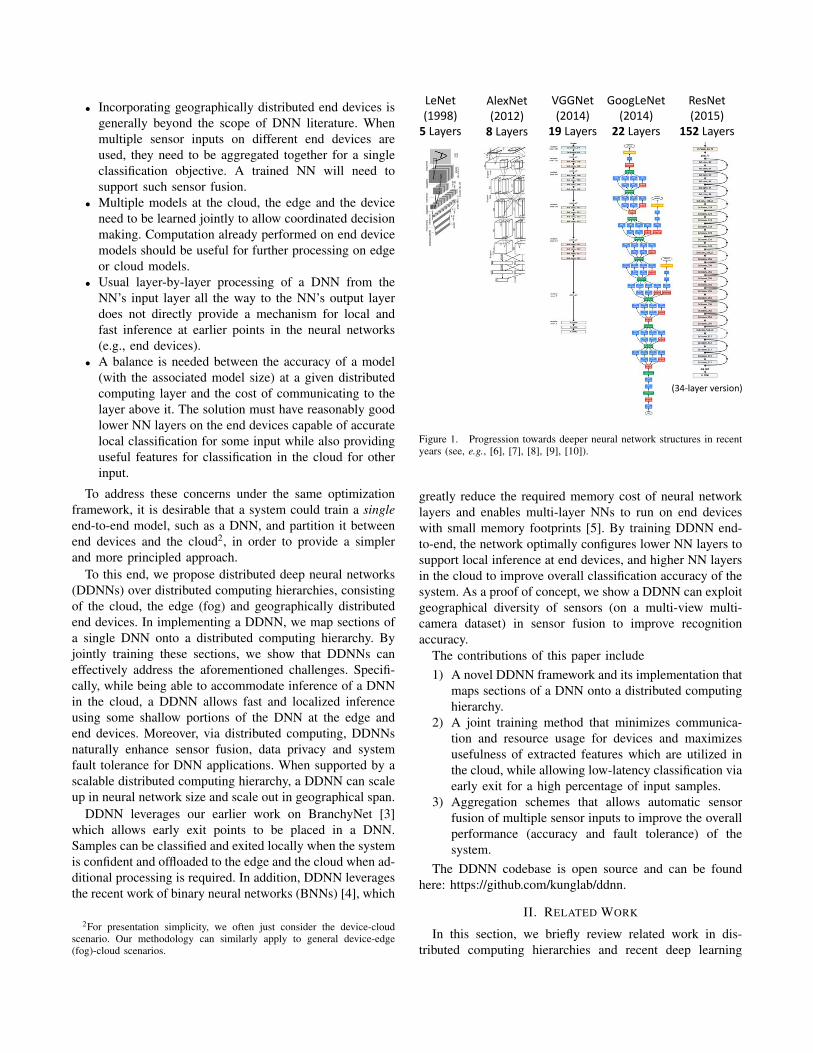
Neural networks (NNs), and deep neural networks(DNNs) in particular, have achieved great success in numer-ous applications in recent years. For example, deep Con-volutional Neural Networks (CNNs) continuously achievestate-of-the-art performances on various tasks in computervision as shown in Figure 1. At the same time, the numberof end devices, including Internet of Things (IoT) devices,has increased dramatically. These devices are appealingtargets for machine learning applications as they are oftendirectly connected to sensors (e.g., cameras, microphones,gyroscopes) that capture a large quantity of input data in astreaming fashion.
However, the current state of machine learning systemson end devices leaves an unsatisfactory choice: either (1)offload input sensor data to large NN models (e.g., DNNs) inthe cloud, with the associated communication costs, latency
issues and privacy concerns, or (2) perform classificationdirectly on the end device using simple Machine Learning(ML) models e.g., linear Support Vector Machine (SVM),leading to reduced system accuracy.
To address these shortcomings, it is natural to considerthe use of a distributed computing approach. Hierarchicallydistributed computing structures consisting of the cloud,the edge and devices (see, e.g., [1], [2]) have inherentadvantages, such as supporting coordinated central and localdecisions, and providing system scalability, for large-scaleintelligent tasks based on geographically distributed IoTdevices.
An example of one such distributed approach is to com-bine a small NN1 model (less number of parameters) on enddevices and a larger NN model (more number of parameters)in the cloud. The small model at an end device can quicklyperform initial feature extraction, and also classification ifthe model is confident. Otherwise, the end device can fallback to the large NN model in the cloud, which performsfurther processing and final classification. This approachhas the benefit of low communication costs compared toalways offloading NN input to the cloud and can achievehigher accuracy compared to a simple model on device.Additionally, since a summary based on extracted featuresfrom the end device model are sent instead of raw sensordata, the system could provide better privacy protection.
However, this kind of distributed approach over a com-puting hierarchy is challenging for a number of reasons,including:
• End devices such as embedded sensor nodes often havelimited memory and battery budgets. This makes it anissue to fit models on the devices that meet the requiredaccuracy and energy constraints.
• A straightforward partitioning of NN models over acomputing hierarchy may incur prohibitively large com-munication costs in transferring intermediate resultsbetween computation nodes.
1The term network layer may refer to either a layer in a NN or a layerin the distributed computing hierarchy (e.g., edge or cloud). In order toremove ambiguity, when we refer to network layers for NN we explicitlyuse the term NN layers.
• Incorporating geographically distributed end devices isgenerally beyond the scope of DNN literature. Whenmultiple sensor inputs on different end devices areused, they need to be aggregated together for a singleclassification objective. A trained NN will need tosupport such sensor fusion.
• Multiple models at the cloud, the edge and the deviceneed to be learned jointly to allow coordinated decisionmaking. Computation already performed on end devicemodels should be useful for further processing on edgeor cloud models.
• Usual layer-by-layer processing of a DNN from theNN’s input layer all the way to the NN’s output layerdoes not directly provide a mechanism for local andfast inference at earlier points in the neural networks(e.g., end devices).
• A balance is needed between the accuracy of a model(with the associated model size) at a given distributedcomputing layer and the cost of communicating to thelayer above it. The solution must have reasonably goodlower NN layers on the end devices capable of accuratelocal classification for some input while also providinguseful features for classification in the cloud for otherinput.
To address these concerns under the same optimizationframework, it is desirable that a system could train a singleend-to-end model, such as a DNN, and partition it betweenend devices and the cloud2, in order to provide a simplerand more principled approach.
To this end, we propose distributed deep neural networks(DDNNs) over distributed computing hierarchies, consistingof the cloud, the edge (fog) and geographically distributedend devices. In implementing a DDNN, we map sections ofa single DNN onto a distributed computing hierarchy. Byjointly training these sections, we show that DDNNs caneffectively address the aforementioned challenges. Specifi-cally, while being able to accommodate inference of a DNNin the cloud, a DDNN allows fast and localized inferenceusing some shallow portions of the DNN at the edge andend devices. Moreover, via distributed computing, DDNNsnaturally enhance sensor fusion, data privacy and systemfault tolerance for DNN applications. When supported by ascalable distributed computing hierarchy, a DDNN can scaleup in neural network size and scale out in geographical span.
DDNN leverages our earlier work on BranchyNet [3]which allows early exit points to be placed in a DNN.Samples can be classified and exited locally when the systemis confident and offloaded to the edge and the cloud when ad-ditional processing is required. In addition, DDNN leveragesthe recent work of binary neural networks (BNNs) [4], which
2For presentation simplicity, we often just consider the device-cloudscenario. Our methodology can similarly apply to general device-edge(fog)-cloud scenarios.
LeNet(1998)
5 Layers
AlexNet(2012)
8 Layers
VGGNet(2014)
19 Layers
GoogLeNet(2014)
22 Layers
ResNet(2015)
152 Layers
(34-layer version)
Figure 1. Progression towards deeper neural network structures in recentyears (see, e.g., [6], [7], [8], [9], [10]).
greatly reduce the required memory cost of neural networklayers and enables multi-layer NNs to run on end deviceswith small memory footprints [5]. By training DDNN end-to-end, the network optimally configures lower NN layers tosupport local inference at end devices, and higher NN layersin the cloud to improve overall classification accuracy of thesystem. As a proof of concept, we show a DDNN can exploitgeographical diversity of sensors (on a multi-view multi-camera dataset) in sensor fusion to improve recognitionaccuracy.
The contributions of this paper include1) A novel DDNN framework and its implementation that
maps sections of a DNN onto a distributed computinghierarchy.
2) A joint training method that minimizes communica-tion and resource usage for devices and maximizesusefulness of extracted features which are utilized inthe cloud, while allowing low-latency classification viaearly exit for a high percentage of input samples.
3) Aggregation schemes that allows automatic sensorfusion of multiple sensor inputs to improve the overallperformance (accuracy and fault tolerance) of thesystem.
The DDNN codebase is open source and can be foundhere: https://github.com/kunglab/ddnn.
II. RELATED WORK
In this section, we briefly review related work in dis-tributed computing hierarchies and recent deep learning
algorithms that enable our proposed method to run in a dis-tributed fashion. We then discuss other approaches involvingdistributed deep networks.
A. Distributed Computing Hierarchy
The framework of a large-scale distributed computinghierarchy has assumed new significance in the emerging eraof IoT. It is widely expected that most of data generatedby the massive number of IoT devices must be processedlocally at the devices or at the edge, for otherwise thetotal amount of sensor data for a centralized cloud wouldoverwhelm the communication network bandwidth. In addi-tion, a distributed computing hierarchy offers opportunitiesfor system scalability, data security and privacy, as well asshorter response times (see, e.g., [2], [11]). For example,in [11], a face recognition application shows a reducedresponse time is achieved when a smartphone’s photos areproceeded by the edge (fog) as opposed to the cloud. In thispaper, we show that DDNN can systematically exploit theinherent advantages of a distributed computing hierarchy forDNN applications and achieve similar benefits.
B. Deep Neural Network Extensions
Binarized neural networks (BNNs) are a recent type ofneural networks, where the weights in linear and convolu-tional layers are constrained to {−1, 1} (stored as 0 and 1respectively). This representation has been shown to achievesimilar classification accuracy for some datasets such asMNIST and CIFAR-10 [12] when compared to a standardfloating-point neural network while using less memory andreduced computation due to the binary format [4]. Embeddedbinarized neural networks (eBNNs) extends BNNs to allowthe network to fit on embedded devices by reducing floating-point temporaries through reordering the operations in in-ference [5]. These compact models are especially attractivein end device settings, where memory can be a limitingfactor and low power consumption is required. In DDNN,we use BNNs, eBNNs and the alike to accommodate theend devices, so that they can be jointly trained with the NNlayers in the edge and cloud.
BranchyNet proposed a solution of classifying samples atearlier points in a neural network, called early exit points,through the use of an entropy-based confidence criteria [3].If at an early exit point a sample is deemed confident basedon the entropy of the computed probability vector for targetclasses, then it is classified and no further computation isperformed by the higher NN layers. In DDNN, exit pointsare placed at physical boundaries (e.g., between the last NNlayer on an end device and the first NN layer in the nexthigher layer of the distributed computing hierarchy suchas the edge or the cloud). Input samples that can alreadybe classified early will exit locally, thereby achieving alowered response latency and saving communication to thenext physical boundary. With similar objectives, SACT [13]
allocates computation on a per region basis in an image, andexits each region independently when it is deemed to be ofsufficient quality.
C. Distributed Training of Deep Networks
Current research on distributing deep networks is mainlyfocused on improving the runtime of training the neuralnetwork. In 2012, Dean et al. proposed DistBelief, whichmaps large DNNs over thousands of CPU cores duringtraining [14]. More recently, several methods have beenproposed to scale up DNN training across GPU clusters [15],[16], which further reduces the runtime of network training.Note that this form of distributing DNNs (over homogeneouscomputing units) is fundamentally different from the notionpresented in this paper. We proposes a way to train andperform feedforward inference over deep networks that canbe deployed over a distributed computing hierarchy, ratherthan processed in parallel over bus- or switch-connectedCPUs or GPUs in the cloud.
III. PROPOSED DISTRIBUTED DEEP NEURAL NETWORKS
In this section we give an overview of the proposeddistributed deep neural network (DDNN) architecture anddescribe how training and inference in DDNN is performed.
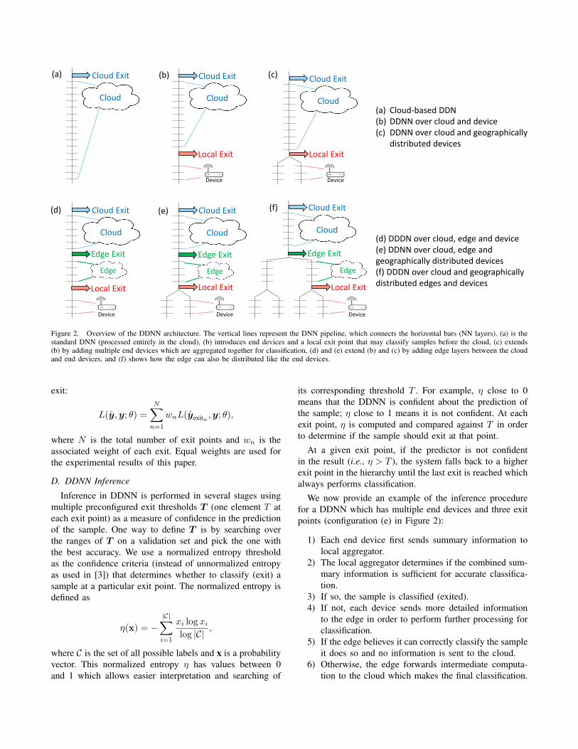
A. DDNN Architecture
DDNN maps a trained DNN onto heterogeneous physicaldevices distributed locally, at the edge, and in the cloud.Since DDNN relies on a jointly trained DNN framework atall parts in the neural network, for both training and infer-ence, many of the difficult engineering decisions are greatlysimplified. Figure 2 provides an overview of the DDNNarchitecture. The configurations presented show how DDNNcan scale the inference computation across different physicaldevices. The cloud-based DDNN in (a) can be viewed asthe standard DNN running in the cloud as described inthe introduction. In this case, sensor input captured on enddevices is sent to the cloud in original format (raw inputformat), where all layers of DNN inference is performed.
We can extend this model to include a single end device,as shown in (b), by performing a portion of the DNNinference computation on the device rather than sending theraw input to the cloud. Using an exit point after deviceinference, we may classify those samples which the localnetwork is confident about, without sending any informationto the cloud. For more difficult cases, the intermediate DNNoutput (up to the local exit) is sent to the cloud, wherefurther inference is performed using additional NN layersand a final classification decision is made. Note that theintermediate output can be designed to be much smaller thanthe sensor input (e.g., a raw image from a video camera),and therefore drastically reduce the network communicationrequired between the end device and the cloud. The details
of how communication is considered in the network isdiscussed in section III-E.
DDNN can also be extended to multiple end deviceswhich may be geographically distributed, shown in (c),that work together to make a classification decision. Here,each end device performs local computation as in (b), buttheir output is aggregated together before the local exitpoint. Since the entire DDNN is jointly trained acrossall end devices and exit points, the network automaticallyaggregates the input with the objective of achieving max-imum classification accuracy. This automatic data fusion(sensor fusion) simplifies runtime inference by avoiding thenecessity of manually combining output from multiple enddevices. We will discuss the design of feature aggregationin detail in section III-B. As before, if the local exit pointis not confident about the sample, each end devices sendsintermediate output to the cloud, where another round offeature aggregation is performed before making a finalclassification decision.
DDNN scales vertically as well, by using an edge layer inthe distributed computing hierarchy between the end devicesand cloud, shown in (d) and (e). The edge acts similarly tothe cloud, by taking output from the end devices, performingaggregation and classification if possible, and forwarding itsown intermediate output to the cloud if more processing isneeded. In this way, DDNN naturally adjusts the networkcommunication and response time of the system on a persample basis. Samples that can be correctly classified locallyare exiting without any communication to the edge or cloud.Samples that require more feature extraction than can be pro-vided locally are sent to the edge, and eventually the cloudif necessary. Finally, DDNNs can also scale geographicallyacross the edge layer as well, which is shown in (f).
B. DDNN Aggregation Methods
In DDNN configurations with multiple end devices(e.g., (c), (e), and (f) in Figure 2), the output from each enddevice must be aggregated in order to perform classification.We present several different schemes for aggregating theoutput. Each aggregation method makes different assump-tions about how the device output should be combined andtherefore can result in different system accuracy. We presentthree approaches:
• Max pooling (MP). MP aggregates the input vectorsby taking the max of each component. Mathematically,max pooling can be written as
vj = max1≤i≤n
vij ,
where n is the number of inputs and vij is the j-th component of the input vector and vj is the j-thcomponent of the resulting output vector.
• Average pooling (AP). AP aggregates the input vectorsby taking the average of each component. This is
written as
vj =
n∑i=1
vijn
,
where n is the number of inputs and vij is the j-th component of the input vector and vj is the j-thcomponent of the resulting output vector. Averagingmay reduce noisy input presented in some end devices.
• Concatenation (CC). CC simply concatenates the inputvectors together. CC retains all information which isuseful for higher layers (e.g., the cloud) that can usethe full information to extract higher level features.Note that this expands the dimension of the resultingvector. To map this vector back to the same numberof dimensions as input vectors, we add an additionallinear layer.
We analyzes these aggregation methods in Section IV-C.
C. DDNN Training
While DDNN inference is distributed over the distributedcomputing hierarchy, the DDNN system can be trained on asingle powerful server or in the cloud. One aspect of DDNNthat is different from most conventional DNN pipelines is theuse of multiple exit points as shown in Figure 2. At trainingtime, the loss from each exit is combined during back-propagation so that the entire network can be jointly trained,and each exit point achieves good accuracy relative to itsdepth. For this work, we follow joint training as describedin GoogleNet [9] and BranchyNet [3].
For the system evaluation discussed in Section IV, weapply DDNNs to a classification task. We use the softmaxcross entropy loss function as the optimization objective.We now describe formally how we train DDNNs. Let y bea one-hot ground-truth label vector, x be an input sampleand C be the set of all possible labels. For each exit, thesoftmax cross entropy objective function can be written as
L(y,y; θ) =− 1
|C|∑c∈C
yc log yc,
where
y = softmax(z) =exp(z)∑
c∈C
exp(zc),
and
z =fexitn(x; θ),
where fexitn is a function representing the computation ofthe neural network layers from an entry point to the n-thexit branch and θ represents the network parameters such asweights and biases of those layers.
To train the DDNN we form a joint optimization problemas minimizing a weighted sum of the loss functions of each
Cloud Exit Cloud Exit Cloud Exit
Cloud Exit Cloud Exit
Cloud
Cloud Exit
CloudCloud
Cloud Cloud Cloud
Local Exit Local Exit
Device Device
Local Exit
Device
Local Exit
Device
Local Exit
Device
Edge Exit
Edge
Edge Exit
Edge
Edge Exit
Edge
(a) (b) (c)
(f)(e)(d)
(a) Cloud-based DDN(b) DDNN over cloud and device(c) DDNN over cloud and geographically
distributed devices
(d) DDDN over cloud, edge and device(e) DDNN over cloud, edge and geographically distributed devices(f) DDDN over cloud and geographically distributed edges and devices
Figure 2. Overview of the DDNN architecture. The vertical lines represent the DNN pipeline, which connects the horizontal bars (NN layers). (a) is thestandard DNN (processed entirely in the cloud), (b) introduces end devices and a local exit point that may classify samples before the cloud, (c) extends(b) by adding multiple end devices which are aggregated together for classification, (d) and (e) extend (b) and (c) by adding edge layers between the cloudand end devices, and (f) shows how the edge can also be distributed like the end devices.
exit:
L(y,y; θ) =
N∑n=1
wnL(yexitn ,y; θ),
where N is the total number of exit points and wn is theassociated weight of each exit. Equal weights are used forthe experimental results of this paper.
D. DDNN Inference
Inference in DDNN is performed in several stages usingmultiple preconfigured exit thresholds T (one element T ateach exit point) as a measure of confidence in the predictionof the sample. One way to define T is by searching overthe ranges of T on a validation set and pick the one withthe best accuracy. We use a normalized entropy thresholdas the confidence criteria (instead of unnormalized entropyas used in [3]) that determines whether to classify (exit) asample at a particular exit point. The normalized entropy isdefined as
η(x) = −|C|∑i=1
xi log xi
log |C|,
where C is the set of all possible labels and x is a probabilityvector. This normalized entropy η has values between 0and 1 which allows easier interpretation and searching of
its corresponding threshold T . For example, η close to 0means that the DDNN is confident about the prediction ofthe sample; η close to 1 means it is not confident. At eachexit point, η is computed and compared against T in orderto determine if the sample should exit at that point.
At a given exit point, if the predictor is not confidentin the result (i.e., η > T ), the system falls back to a higherexit point in the hierarchy until the last exit is reached whichalways performs classification.
We now provide an example of the inference procedurefor a DDNN which has multiple end devices and three exitpoints (configuration (e) in Figure 2):
1) Each end device first sends summary information tolocal aggregator.
2) The local aggregator determines if the combined sum-mary information is sufficient for accurate classifica-tion.
3) If so, the sample is classified (exited).4) If not, each device sends more detailed information
to the edge in order to perform further processing forclassification.
5) If the edge believes it can correctly classify the sampleit does so and no information is sent to the cloud.
6) Otherwise, the edge forwards intermediate computa-tion to the cloud which makes the final classification.
E. Communication Cost of DDNN Inference
The total communication cost for an end device with thelocal and cloud aggregator is calculated as
c = 4× |C|+ (1− l)f × o
8(1)
where l is the percentage of samples exited locally, C is theset of all possible labels (3 in our experiments), f is thenumber of filters, and o is the output size of a single filterfor the final NN layer on the end-device. The constant 4corresponds to 4 bytes which are used to represent a floating-point number and the constant 8 corresponds to bits usedto express a byte output. The first term assumes a singlefloating-point per class, which conveys the probability thatthe sample to be transmitted from the end device to the localaggregator belongs to this class. This step happens regardlessof whether the sample is exited locally or at a later exit point.The second term is the communication between end deviceand cloud which happens (1− l) fraction of the time, whenthe sample is exited in the cloud rather than locally.
F. Accuracy Measures
Throughout the evaluation in Section IV, we use differentaccuracy measures for the various exit points in a DDNN asfollows:
• Local Accuracy is the accuracy when exiting 100% ofsamples at the local exit of a DDNN.
• Edge Accuracy is the accuracy when exiting 100% ofsamples at the edge exit of a DDNN.
• Cloud Accuracy is the accuracy when exiting 100% ofsamples at the cloud exit of a DDNN.
• Overall Accuracy is the accuracy when exiting somepercentage of samples at each exit point in the hier-archy. The samples classified at each exit point aredetermined by the entropy threshold T for that exit.The impact of T on classification accuracy and com-munication cost is discussed in Section IV-D.
• Individual Accuracy is the accuracy of an end deviceNN model trained separately from DDNN. The NNmodel for each end device consists of a ConvP blockfollowed by a FC block (a single end device portionas shown in Figure 4). In the evaluation, individualaccuracy for each device is computed by classifying allsamples using the individual NN model and not relyingon the local or cloud exit points of a DDNN.
IV. DDNN SYSTEM EVALUATION
In this section, we evaluate DDNN on a scenario withmultiple end devices and demonstrate the following charac-teristics of the approach:
• DDNNs allow multiple end devices to work collabo-ratively in order to improve accuracy at both the localand cloud exit points.
• DDNNs seamlessly extend the capability of end devicesby offloading difficult samples to the cloud.
• DDNNs have built-in fault tolerance. We illustrate thatmissing any single end device does not dramaticallyaffect the accuracy of the system. Additionally, weshow how performance gradually degrades as more enddevices are lost.
• DDNNs reduce communication costs for end devicescompared to traditional system that offloads all inputsensor data to the cloud.
We first introduce the DDNN architecture and dataset usedin our evaluation.
A. DDNN Evaluation Architecture
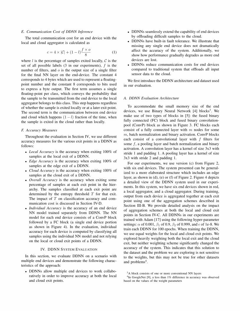
To accommodate the small memory size of the enddevices, we use Binary Neural Network [4] blocks3. Wemake use of two types of blocks in [5]: the fused binaryfully connected (FC) block and fused binary convolution-pool (ConvP) block as shown in Figure 3. FC blocks eachconsist of a fully connected layer with m nodes for somem, batch normalization and binary activation. ConvP blockseach consist of a convolutional layer with f filters forsome f , a pooling layer and batch normalization and binaryactivation. A convolution layer has a kernel of size 3x3 withstride 1 and padding 1. A pooling layer has a kernel of size3x3 with stride 2 and padding 1.
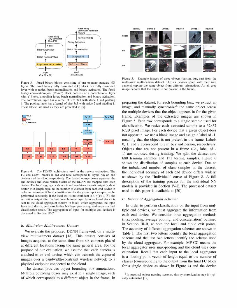
For our experiments, we use version (c) from Figure 2,with six end devices. The system presented can be general-ized to a more elaborated structure which includes an edgelayer, as shown in (d), (e) or (f) of Figure 2. Figure 4 depictsa detailed view of the DDNN system used in our experi-ments. In this system, we have six end devices shown in red,a local aggregator, and a cloud aggregator. During training,output from each device is aggregated together at each exitpoint using one of the aggregation schemes described inSection III-B. We provide detailed analysis on the impactof aggregation schemes at both the local and cloud exitpoints in Section IV-C. All DDNNs in our experiments aretrained with Adam [17] using the following hyper-parametersettings: α of 0.001, β1 of 0.9, β2 of 0.999, and ϵ of 1e-8. Wetrain each DDNN for 100 epochs. When training the DDNN,we use equal weights for the local and cloud exit points. Weexplored heavily weighting both the local exit and the cloudexit, but neither weighting scheme significantly changed theaccuracy of the system. This indicates that this solution tothe dataset and the problem we are exploring is not sensitiveto the weights, but this may not be true for other datasetsand problems4.
3A block consists of one or more conventional NN layers4In GoogleNet [9], a less than 1% difference in accuracy was observed
based on the values of the weight parameters
3x3 conv, f filters
Binary Activation
Batch Normalization
f x 16 x 16 bits
Fused Binary Convolution-Pool Block (ConvP)
3x3 pool, /2
input (3 x 32 x 32)
fully-connected, n nodes
Binary Activation
Batch Normalization
n bits
Fused Binary Fully-Connected Block (FC)
input (3 x 32 x 32)
Figure 3. Fused binary blocks consisting of one or more standard NNlayers. The fused binary fully connected (FC) block is a fully connectedlayer with n nodes, batch normalization and binary activation. The fusedbinary convolution-pool (ConvP) block consists of a convolutional layerwith f filters, a pooling layer, batch normalization and binary activation.The convolution layer has a kernel of size 3x3 with stride 1 and padding1. The pooling layer has a kernel of size 3x3 with stride 2 and padding 1.These blocks are used as they are presented in [5].
Figure 4. The DDNN architecture used in the system evaluation. TheFC and ConvP blocks in red and blue correspond to layers run on enddevices and the cloud respectively. The dashed orange boxes represent theend devices and show which blocks of the DDNN are mapped onto eachdevice. The local aggregator shown in red combines the exit output (a shortvector with length equal to the number of classes) from each end device inorder to determine if local classification for the given input sample can beperformed accurately. If the local exit is not confident (i.e. η(x) > T ), theactivation output after the last convolutional layer from each end device issent to the cloud aggregator (shown in blue), which aggregates the inputfrom each device, performs further NN layer processing, and outputs a finalclassification result. The aggregation of input for multiple end devices isdiscussed in Section IV-C.
B. Multi-view Multi-camera Dataset
We evaluate the proposed DDNN framework on a multi-view multi-camera dataset [18]. This dataset consists ofimages acquired at the same time from six cameras placedat different locations facing the same general area. For thepurpose of our evaluation, we assume that each camera isattached to an end device, which can transmit the capturedimages over a bandwidth-constraint wireless network to aphysical endpoint connected to the cloud.
The dataset provides object bounding box annotations.Multiple bounding boxes may exist in a single image, eachof which corresponds to a different object in the frame. In
Device 1 Device 2 Device 3 Device 4 Device 5 Device 6
Person
Bus
Car
Figure 5. Example images of three objects (person, bus, car) from themulti-view multi-camera dataset. The six devices (each with their owncamera) capture the same object from different orientations. An all greyimage denotes that the object is not present in the frame.
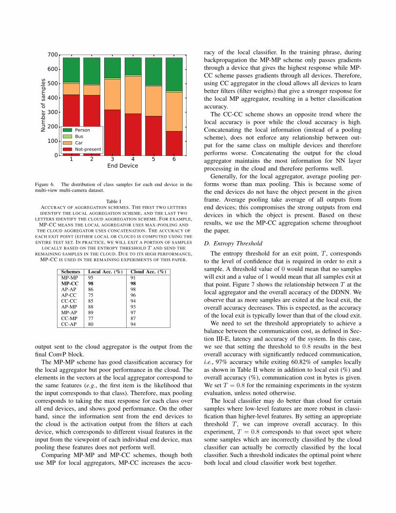
preparing the dataset, for each bounding box, we extract animage, and manually synchronize5 the same object acrossthe multiple devices that the object appears in for the givenframe. Examples of the extracted images are shown inFigure 5. Each row corresponds to a single sample used forclassification. We resize each extracted sample to a 32x32RGB pixel image. For each device that a given object doesnot appear in, we use a blank image and assign a label of -1,meaning that the object is not present in the frame. Labels0, 1, and 2 correspond to car, bus and person, respectively.Objects that are not present in a frame (i.e., label of -1) are not used during training. We split the dataset into680 training samples and 171 testing samples. Figure 6shows the distribution of samples at each device. Due tothe imbalanced number of class samples in the dataset,the individual accuracy of each end device differs widely,as shown by the “Individual” curve of Figure 8. A fulldescription of the training process for the individual NNmodels is provided in Section IV-E. The processed datasetused in this paper is available at [20].
C. Impact of Aggregation Schemes
In order to perform classification on the input from mul-tiple end devices, we must aggregate the information fromeach end device. We consider three aggregation methods(max pooling, average pooling, and concatenation) outlinedin Section III-B, at both the local and cloud exit points.The accuracy of different aggregation schemes are shown inTable I. The first two letters identify the local aggregationscheme and the last two letters identify the scheme usedby the cloud aggregator. For example, MP-CC means thelocal aggregator uses max-pooling and the cloud uses con-catenation. Recall that each input to the local aggregatoris a floating-point vector of length equal to the number ofclasses (corresponding to the output from the final FC blockfor a single device as shown in Figure 4) and the device
5In practical object tracking systems, this synchronization step is typi-cally automated [19].
1 2 3 4 5 6End Device
0
100
200
300
400
500
600
700
Num
ber
of
sam
ple
s
Person
Bus
Car
Not-present
Figure 6. The distribution of class samples for each end device in themulti-view multi-camera dataset.
Table IACCURACY OF AGGREGATION SCHEMES. THE FIRST TWO LETTERSIDENTIFY THE LOCAL AGGREGATION SCHEME, AND THE LAST TWO
LETTERS IDENTIFY THE CLOUD AGGREGATION SCHEME. FOR EXAMPLE,MP-CC MEANS THE LOCAL AGGREGATOR USES MAX-POOLING AND
THE CLOUD AGGREGATOR USES CONCATENATION. THE ACCURACY OFEACH EXIT POINT (EITHER LOCAL OR CLOUD) IS COMPUTED USING THEENTIRE TEST SET. IN PRACTICE, WE WILL EXIT A PORTION OF SAMPLES
LOCALLY BASED ON THE ENTROPY THRESHOLD T AND SEND THEREMAINING SAMPLES IN THE CLOUD. DUE TO ITS HIGH PERFORMANCE,
MP-CC IS USED IN THE REMAINING EXPERIMENTS OF THIS PAPER.
Schemes Local Acc. (%) Cloud Acc. (%)MP-MP 95 91MP-CC 98 98AP-AP 86 98AP-CC 75 96CC-CC 85 94AP-MP 88 93MP-AP 89 97CC-MP 77 87CC-AP 80 94
output sent to the cloud aggregator is the output from thefinal ConvP block.
The MP-MP scheme has good classification accuracy forthe local aggregator but poor performance in the cloud. Theelements in the vectors at the local aggregator correspond tothe same features (e.g., the first item is the likelihood thatthe input corresponds to that class). Therefore, max poolingcorresponds to taking the max response for each class overall end devices, and shows good performance. On the otherhand, since the information sent from the end devices tothe cloud is the activation output from the filters at eachdevice, which corresponds to different visual features in theinput from the viewpoint of each individual end device, maxpooling these features does not perform well.
Comparing MP-MP and MP-CC schemes, though bothuse MP for local aggregators, MP-CC increases the accu-
racy of the local classifier. In the training phrase, duringbackpropagation the MP-MP scheme only passes gradientsthrough a device that gives the highest response while MP-CC scheme passes gradients through all devices. Therefore,using CC aggregator in the cloud allows all devices to learnbetter filters (filter weights) that give a stronger response forthe local MP aggregator, resulting in a better classificationaccuracy.
The CC-CC scheme shows an opposite trend where thelocal accuracy is poor while the cloud accuracy is high.Concatenating the local information (instead of a poolingscheme), does not enforce any relationship between out-put for the same class on multiple devices and thereforeperforms worse. Concatenating the output for the cloudaggregator maintains the most information for NN layerprocessing in the cloud and therefore performs well.
Generally, for the local aggregator, average pooling per-forms worse than max pooling. This is because some ofthe end devices do not have the object present in the givenframe. Average pooling take average of all outputs fromend devices; this compromises the strong outputs from enddevices in which the object is present. Based on theseresults, we use the MP-CC aggregation scheme throughoutthe paper.
D. Entropy Threshold
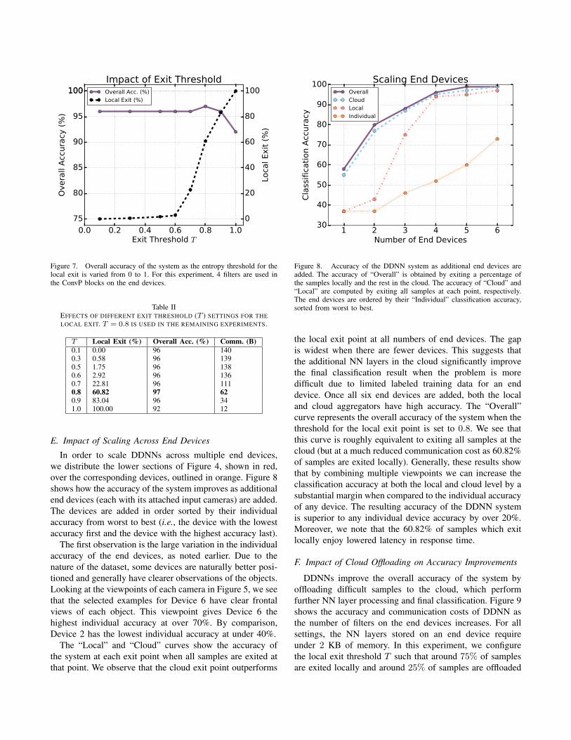
The entropy threshold for an exit point, T , correspondsto the level of confidence that is required in order to exit asample. A threshold value of 0 would mean that no sampleswill exit and a value of 1 would mean that all samples exit atthat point. Figure 7 shows the relationship between T at thelocal aggregator and the overall accuracy of the DDNN. Weobserve that as more samples are exited at the local exit, theoverall accuracy decreases. This is expected, as the accuracyof the local exit is typically lower than that of the cloud exit.
We need to set the threshold appropriately to achieve abalance between the communication cost, as defined in Sec-tion III-E, latency and accuracy of the system. In this case,we see that setting the threshold to 0.8 results in the bestoverall accuracy with significantly reduced communication,i.e., 97% accuracy while exiting 60.82% of samples locallyas shown in Table II where in addition to local exit (%) andoverall accuracy (%), communication cost in bytes is given.We set T = 0.8 for the remaining experiments in the systemevaluation, unless noted otherwise.
The local classifier may do better than cloud for certainsamples where low-level features are more robust in classi-fication than higher-level features. By setting an appropriatethreshold T , we can improve overall accuracy. In thisexperiment, T = 0.8 corresponds to that sweet spot wheresome samples which are incorrectly classified by the cloudclassifier can actually be correctly classified by the localclassifier. Such a threshold indicates the optimal point whereboth local and cloud classifier work best together.
0.0 0.2 0.4 0.6 0.8 1.0Exit Threshold T
75
80
85
90
95
100100
Overa
ll A
ccura
cy (
%)
Impact of Exit ThresholdOverall Acc. (%)
Local Exit (%)
0
20
40
60
80
100
Loca
l Exit
(%
)Figure 7. Overall accuracy of the system as the entropy threshold for thelocal exit is varied from 0 to 1. For this experiment, 4 filters are used inthe ConvP blocks on the end devices.
Table IIEFFECTS OF DIFFERENT EXIT THRESHOLD (T ) SETTINGS FOR THELOCAL EXIT. T = 0.8 IS USED IN THE REMAINING EXPERIMENTS.
T Local Exit (%) Overall Acc. (%) Comm. (B)0.1 0.00 96 1400.3 0.58 96 1390.5 1.75 96 1380.6 2.92 96 1360.7 22.81 96 1110.8 60.82 97 620.9 83.04 96 341.0 100.00 92 12
E. Impact of Scaling Across End Devices
In order to scale DDNNs across multiple end devices,we distribute the lower sections of Figure 4, shown in red,over the corresponding devices, outlined in orange. Figure 8shows how the accuracy of the system improves as additionalend devices (each with its attached input cameras) are added.The devices are added in order sorted by their individualaccuracy from worst to best (i.e., the device with the lowestaccuracy first and the device with the highest accuracy last).
The first observation is the large variation in the individualaccuracy of the end devices, as noted earlier. Due to thenature of the dataset, some devices are naturally better posi-tioned and generally have clearer observations of the objects.Looking at the viewpoints of each camera in Figure 5, we seethat the selected examples for Device 6 have clear frontalviews of each object. This viewpoint gives Device 6 thehighest individual accuracy at over 70%. By comparison,Device 2 has the lowest individual accuracy at under 40%.
The “Local” and “Cloud” curves show the accuracy ofthe system at each exit point when all samples are exited atthat point. We observe that the cloud exit point outperforms
1 2 3 4 5 6Number of End Devices
30
40
50
60
70
80
90
100
Cla
ssific
ati
on A
ccura
cy
Scaling End DevicesOverall
Cloud
Local
Individual
Figure 8. Accuracy of the DDNN system as additional end devices areadded. The accuracy of “Overall” is obtained by exiting a percentage ofthe samples locally and the rest in the cloud. The accuracy of “Cloud” and“Local” are computed by exiting all samples at each point, respectively.The end devices are ordered by their “Individual” classification accuracy,sorted from worst to best.
the local exit point at all numbers of end devices. The gapis widest when there are fewer devices. This suggests thatthe additional NN layers in the cloud significantly improvethe final classification result when the problem is moredifficult due to limited labeled training data for an enddevice. Once all six end devices are added, both the localand cloud aggregators have high accuracy. The “Overall”curve represents the overall accuracy of the system when thethreshold for the local exit point is set to 0.8. We see thatthis curve is roughly equivalent to exiting all samples at thecloud (but at a much reduced communication cost as 60.82%of samples are exited locally). Generally, these results showthat by combining multiple viewpoints we can increase theclassification accuracy at both the local and cloud level by asubstantial margin when compared to the individual accuracyof any device. The resulting accuracy of the DDNN systemis superior to any individual device accuracy by over 20%.Moreover, we note that the 60.82% of samples which exitlocally enjoy lowered latency in response time.
F. Impact of Cloud Offloading on Accuracy Improvements
DDNNs improve the overall accuracy of the system byoffloading difficult samples to the cloud, which performfurther NN layer processing and final classification. Figure 9shows the accuracy and communication costs of DDNN asthe number of filters on the end devices increases. For allsettings, the NN layers stored on an end device requireunder 2 KB of memory. In this experiment, we configurethe local exit threshold T such that around 75% of samplesare exited locally and around 25% of samples are offloaded
15 20 25 30Communication (B)
84
86
88
90
92
94
96
98
100
Cla
ssific
ati
on A
ccura
cy
Overall Acc.
Cloud Acc.
Local Acc.
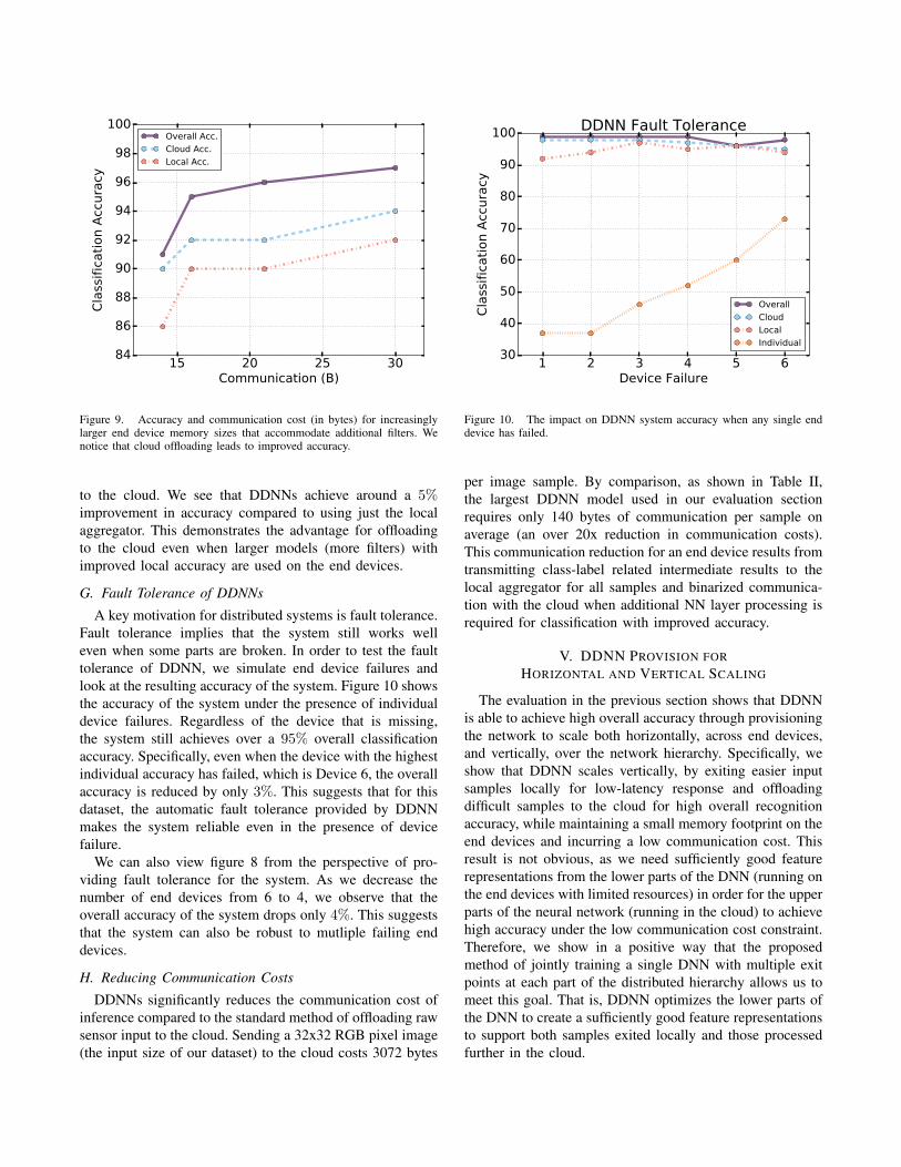
Figure 9. Accuracy and communication cost (in bytes) for increasinglylarger end device memory sizes that accommodate additional filters. Wenotice that cloud offloading leads to improved accuracy.
to the cloud. We see that DDNNs achieve around a 5%improvement in accuracy compared to using just the localaggregator. This demonstrates the advantage for offloadingto the cloud even when larger models (more filters) withimproved local accuracy are used on the end devices.
G. Fault Tolerance of DDNNs
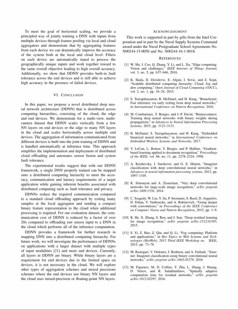
A key motivation for distributed systems is fault tolerance.Fault tolerance implies that the system still works welleven when some parts are broken. In order to test the faulttolerance of DDNN, we simulate end device failures andlook at the resulting accuracy of the system. Figure 10 showsthe accuracy of the system under the presence of individualdevice failures. Regardless of the device that is missing,the system still achieves over a 95% overall classificationaccuracy. Specifically, even when the device with the highestindividual accuracy has failed, which is Device 6, the overallaccuracy is reduced by only 3%. This suggests that for thisdataset, the automatic fault tolerance provided by DDNNmakes the system reliable even in the presence of devicefailure.
We can also view figure 8 from the perspective of pro-viding fault tolerance for the system. As we decrease thenumber of end devices from 6 to 4, we observe that theoverall accuracy of the system drops only 4%. This suggeststhat the system can also be robust to mutliple failing enddevices.
H. Reducing Communication Costs
DDNNs significantly reduces the communication cost ofinference compared to the standard method of offloading rawsensor input to the cloud. Sending a 32x32 RGB pixel image(the input size of our dataset) to the cloud costs 3072 bytes
1 2 3 4 5 6Device Failure
30
40
50
60
70
80
90
100
Cla
ssific
ati
on A
ccura
cy
DDNN Fault Tolerance
Overall
Cloud
Local
Individual
Figure 10. The impact on DDNN system accuracy when any single enddevice has failed.
per image sample. By comparison, as shown in Table II,the largest DDNN model used in our evaluation sectionrequires only 140 bytes of communication per sample onaverage (an over 20x reduction in communication costs).This communication reduction for an end device results fromtransmitting class-label related intermediate results to thelocal aggregator for all samples and binarized communica-tion with the cloud when additional NN layer processing isrequired for classification with improved accuracy.
V. DDNN PROVISION FORHORIZONTAL AND VERTICAL SCALING
The evaluation in the previous section shows that DDNNis able to achieve high overall accuracy through provisioningthe network to scale both horizontally, across end devices,and vertically, over the network hierarchy. Specifically, weshow that DDNN scales vertically, by exiting easier inputsamples locally for low-latency response and offloadingdifficult samples to the cloud for high overall recognitionaccuracy, while maintaining a small memory footprint on theend devices and incurring a low communication cost. Thisresult is not obvious, as we need sufficiently good featurerepresentations from the lower parts of the DNN (running onthe end devices with limited resources) in order for the upperparts of the neural network (running in the cloud) to achievehigh accuracy under the low communication cost constraint.Therefore, we show in a positive way that the proposedmethod of jointly training a single DNN with multiple exitpoints at each part of the distributed hierarchy allows us tomeet this goal. That is, DDNN optimizes the lower parts ofthe DNN to create a sufficiently good feature representationsto support both samples exited locally and those processedfurther in the cloud.
To meet the goal of horizontal scaling, we provide aprincipled way of jointly training a DNN with inputs frommultiple devices through feature pooling via local and cloudaggregators and demonstrate that by aggregating featuresfrom each device we can dramatically improve the accuracyof the system both at the local and cloud level. Filterson each device are automatically tuned to process thegeographically unique inputs and work together toward tothe same overall objective leading to high overall accuracy.Additionally, we show that DDNN provides built-in faulttolerance across the end devices and is still able to achievehigh accuracy in the presence of failed devices.
VI. CONCLUSION
In this paper, we propose a novel distributed deep neu-ral network architecture (DDNN) that is distributed acrosscomputing hierarchies, consisting of the cloud, the edgeand end devices. We demonstrate for a multi-view, multi-camera dataset that DDNN scales vertically from a fewNN layers on end devices or the edge to many NN layersin the cloud and scales horizontally across multiple enddevices. The aggregation of information communicated fromdifferent devices is built into the joint training of DDNN andis handled automatically at inference time. This approachsimplifies the implementation and deployment of distributedcloud offloading and automates sensor fusion and systemfault tolerance.
The experimental results suggest that with our DDNNframework, a single DNN properly trained can be mappedonto a distributed computing hierarchy to meet the accu-racy, communication and latency requirements of a targetapplication while gaining inherent benefits associated withdistributed computing such as fault tolerance and privacy.
DDNNs reduce the required communication comparedto a standard cloud offloading approach by exiting manysamples at the local aggregator and sending a compactbinary feature representation to the cloud when additionalprocessing is required. For our evaluation dataset, the com-munication cost of DDNN is reduced by a factor of over20x compared to offloading raw sensor input to a DNN inthe cloud which performs all of the inference computation.
DDNN provides a framework for further research inmapping DNN into a distributed computing hierarchy. Forfuture work, we will investigate the performance of DDNNson applications with a larger dataset with multiple typesof input modalities [21] and more end devices. Currently,all layers in DDNN are binary. While binary layers are arequirement for end devices due to the limited space ondevices, it is not necessary in the cloud. We will exploreother types of aggregation schemes and mixed precisionsschemes where the end devices use binary NN layers andthe cloud uses mixed-precision or floating-point NN layers.
ACKNOWLEDGMENT
This work is supported in part by gifts from the Intel Cor-poration and in part by the Naval Supply Systems Commandaward under the Naval Postgraduate School Agreements No.N00244-15-0050 and No. N00244-16-1-0018.
REFERENCES
[1] W. Shi, J. Cao, Q. Zhang, Y. Li, and L. Xu, “Edge computing:Vision and challenges,” IEEE Internet of Things Journal,vol. 3, no. 5, pp. 637–646, 2016.
[2] K. Skala, D. Davidovic, E. Afgan, I. Sovic, and Z. Sojat,“Scalable distributed computing hierarchy: Cloud, fog anddew computing,” Open Journal of Cloud Computing (OJCC),vol. 2, no. 1, pp. 16–24, 2015.
[3] S. Teerapittayanon, B. McDanel, and H. Kung, “Branchynet:Fast inference via early exiting from deep neural networks,”in International Conference on Pattern Recognition, 2016.
[4] M. Courbariaux, Y. Bengio, and J.-P. David, “Binaryconnect:Training deep neural networks with binary weights duringpropagations,” in Advances in Neural Information ProcessingSystems, 2015, pp. 3123–3131.
[5] B. McDanel, S. Teerapittayanon, and H. Kung, “Embeddedbinarized neural networks,” in International Conference onEmbedded Wireless Systems and Networks, 2017.
[6] Y. LeCun, L. Bottou, Y. Bengio, and P. Haffner, “Gradient-based learning applied to document recognition,” Proceedingsof the IEEE, vol. 86, no. 11, pp. 2278–2324, 1998.
[7] A. Krizhevsky, I. Sutskever, and G. E. Hinton, “Imagenetclassification with deep convolutional neural networks,” inAdvances in neural information processing systems, 2012, pp.1097–1105.
[8] K. Simonyan and A. Zisserman, “Very deep convolutionalnetworks for large-scale image recognition,” arXiv preprintarXiv:1409.1556, 2014.
[9] C. Szegedy, W. Liu, Y. Jia, P. Sermanet, S. Reed, D. Anguelov,D. Erhan, V. Vanhoucke, and A. Rabinovich, “Going deeperwith convolutions,” in Proceedings of the IEEE Conferenceon Computer Vision and Pattern Recognition, 2015, pp. 1–9.
[10] K. He, X. Zhang, S. Ren, and J. Sun, “Deep residual learningfor image recognition,” arXiv preprint arXiv:1512.03385,2015.
[11] S. Yi, Z. Hao, Z. Qin, and Q. Li, “Fog computing: Platformand applications,” in Hot Topics in Web Systems and Tech-nologies (HotWeb), 2015 Third IEEE Workshop on. IEEE,2015, pp. 73–78.
[12] M. Rastegari, V. Ordonez, J. Redmon, and A. Farhadi, “Xnor-net: Imagenet classification using binary convolutional neuralnetworks,” arXiv preprint arXiv:1603.05279, 2016.
[13] M. Figurnov, M. D. Collins, Y. Zhu, L. Zhang, J. Huang,D. Vetrov, and R. Salakhutdinov, “Spatially adaptivecomputation time for residual networks,” arXiv preprintarXiv:1612.02297, 2016.
[14] J. Dean, G. Corrado, R. Monga, K. Chen, M. Devin, M. Mao,A. Senior, P. Tucker, K. Yang, Q. V. Le et al., “Large scaledistributed deep networks,” in Advances in neural informationprocessing systems, 2012, pp. 1223–1231.
[15] F. N. Iandola, K. Ashraf, M. W. Moskewicz, andK. Keutzer, “Firecaffe: near-linear acceleration of deep neu-ral network training on compute clusters,” arXiv preprintarXiv:1511.00175, 2015.
[16] J. Dean, “Large scale deep learning,” in Keynote GPU Tech-nical Conference, vol. 3, 2015, p. 2015.
[17] D. Kingma and J. Ba, “Adam: A method for stochasticoptimization,” arXiv preprint arXiv:1412.6980, 2014.
[18] G. Roig, X. Boix, H. B. Shitrit, and P. Fua, “Conditionalrandom fields for multi-camera object detection,” in 2011International Conference on Computer Vision. IEEE, 2011,pp. 563–570.
[19] X. Li, W. Hu, C. Shen, Z. Zhang, A. Dick, and A. V. D.Hengel, “A survey of appearance models in visual objecttracking,” ACM transactions on Intelligent Systems and Tech-nology (TIST), vol. 4, no. 4, p. 58, 2013.
[20] B. McDanel, “Multiview multicamera dataset,” https://www.dropbox.com/s/uk8c6iymy8nprc0/MVMC.npz, 2016,accessed: 2016-12-10.
[21] M. Cha, Y. Gwon, and H. Kung, “Multimodal sparserepresentation learning and applications,” arXiv preprintarXiv:1511.06238, 2015.