Cnvlutin: Ineffectual-Neuron-Free Deep NeuralNetwork Computing

Jorge Albericio1 Patrick Judd1 Tayler Hetherington2

Tor Aamodt2 Natalie Enright Jerger1 Andreas Moshovos1

1 University of Toronto 2 University of British Columbia

Abstract—This work observes that a large fraction of thecomputations performed by Deep Neural Networks (DNNs) areintrinsically ineffectual as they involve a multiplication where oneof the inputs is zero. This observation motivates Cnvlutin (CNV),a value-based approach to hardware acceleration that eliminatesmost of these ineffectual operations, improving performance andenergy over a state-of-the-art accelerator with no accuracy loss.CNV uses hierarchical data-parallel units, allowing groups oflanes to proceed mostly independently enabling them to skipover the ineffectual computations. A co-designed data storageformat encodes the computation elimination decisions takingthem off the critical path while avoiding control divergence inthe data parallel units. Combined, the units and the data storageformat result in a data-parallel architecture that maintains wide,aligned accesses to its memory hierarchy and that keeps its datalanes busy. By loosening the ineffectual computation identificationcriterion, CNV enables further performance and energy efficiencyimprovements, and more so if a loss in accuracy is acceptable.Experimental measurements over a set of state-of-the-art DNNsfor image classification show that CNV improves performanceover a state-of-the-art accelerator from 1.24× to 1.55× and by1.37× on average without any loss in accuracy by removingzero-valued operand multiplications alone. While CNV incurs anarea overhead of 4.49%, it improves overall EDP (Energy DelayProduct) and ED2P (Energy Delay Squared Product) on averageby 1.47× and 2.01×, respectively. The average performanceimprovements increase to 1.52× without any loss in accuracy witha broader ineffectual identification policy. Further improvementsare demonstrated with a loss in accuracy.

I. INTRODUCTION

Deep Neural Networks (DNNs) are becoming ubiquitousthanks to their exceptional capacity to extract meaningfulfeatures from complex pieces of information such as text,images, or voice. For example, DNNs and in particular,Convolutional Neural Networks (CNNs) currently offer thebest recognition quality versus alternative object recognitionalgorithms, or image classification. DNN are not new [1],but are currently enjoying a renaissance [2] in part due tothe increase in computing capabilities available in commoditycomputing platforms such as general purpose graphics proces-sors [3].

While current DNNs enjoy several practical applications,it is likely that future DNNs will be larger, deeper, processlarger inputs, and used to perform more intricate classificationtasks at faster speeds, if not in real-time. Accordingly, there isa need to boost hardware compute capability while reducingenergy per operation [4] and to possibly do so for smaller formfactor devices.

Given the importance of DNNs, recent work such as the Di-anNao accelerator family [5], [6] targets hardware accelerationof DNNs. The approach taken by these accelerators exploitsthe computation structure of DNNs. Our work is motivatedby the observation that further opportunities for accelerationexist by also taking into account the content being operatedupon. Specifically, Section II shows that on average 44% ofthe operations performed by the dominant computations inDNNs are products that are undoubtedly ineffectual; one of theoperands is a zero and the result is reduced along with othersusing addition. The fraction of these operations does not varysignificantly across different inputs suggesting that ineffectualproducts may be the result of intrinsic properties of DNNs. Thecorresponding operations occupy compute resources wastingtime and energy across inputs. This result along with thevoluminous body of work on valued-based optimizations insoftware (e.g., constant propagation) and hardware (e.g., cachededuplication [7]) for general purpose processing, motivatesvalue-based DNN acceleration approaches in software andhardware.

We present Cnvlutin1 (CNV), a DNN accelerator that fol-lows a value-based approach to dynamically eliminate mostineffectual multiplications. The presented CNV design im-proves performance and energy over the recently proposedDaDianNao accelerator [6]. CNV targets the convolutionallayers of DNNs which dominate execution time (Sections IIand V-B).

DaDianNao takes advantage of the regular access patternand computation structure of DNNs. It uses wide SIMD(single-instruction multiple-data) units that operate in tandemin groups of hundreds of multiplication lanes. Unfortunately,this organization does not allow the lanes to move indepen-dently and thus prevents them from “skipping over” zero-valued inputs. CNV units decouple these lanes into finer-graingroups. A newly proposed data structure format for storingthe inputs and outputs of the relevant layers is generated on-the-fly and enables the seamless elimination of most zero-operand multiplications. The storage format enables CNV tomove the decisions on which computations to eliminate offthe critical path allowing the seamless elimination of workwithout experiencing control divergence in the SIMD units.The assignment of work to units is modified enabling units to

1The name is derived from removing the o’s from convolution: Cønvølutiøn.

be kept busy most of the time independently of the distributionof zeroes in the input. A simple work dispatch unit maintainswide memory accesses over the on-chip eDRAM buffers.

Once the capability to skip zero-operand multiplicationsis in place, more relaxed ineffectual operation identificationcriteria can be used enabling further improvements with noaccuracy loss and to dynamically trade off accuracy for evenfurther performance and energy efficiency improvements.

CNV’s approach bears similarity to density-time vector ex-ecution [8] and related graphics processor proposals [9], [10],[11], [12], [13], [14] for improving efficiency of control-flowintensive computation. CNV directly examines data valuesrather than skipping computation based upon predicate masks.Owing to the application-specific nature of CNV , its proposedimplementation is also simpler. As Section VI explains, CNValso bears similarity to several sparse matrix representationssharing the goal of encoding only the non-zero elements,but sacrificing any memory footprint savings to maintain theability to perform wide accesses to memory and to assign workat the granularity needed by the SIMD units.

Experimental measurements over a set of state-of-the-artDNNs for image classification show that CNV improvesperformance over a state-of-the-art accelerator from 24% to55% and by 37% on average by targeting zero-valued operandsalone. While CNV incurs an area overhead of 4.49%, it im-proves overall Energy Delay Squared (ED2) and Energy Delay(ED) by 2.01× and 1.47× on average respectively. By loosen-ing the ineffectual operand identification criterion, additionalperformance and energy improvements are demonstrated, moreso if a loss in accuracy is acceptable. Specifically, on averageperformance improvements increase to 1.52× with no loss ofaccuracy by dynamically eliminating operands below a per-layer prespecified threshold. Raising these thresholds furtherallows for larger performance gains by trading-off accuracy.

The rest of this manuscript is organized as follows: Sec-tion II motivates CNV’s value-based approach to accelerationfor DNNs by reporting the fraction of multiplications where aruntime calculated operand is zero. Section III presents the keydesign choice for CNV , that of decoupling the multiplicationlanes in smaller groups by means of an example. Section IVdetails the CNV architecture. Section V reports the exper-imental results. Section VI comments on related work andSection VII concludes.

II. MOTIVATION: PRESENCE OF ZEROES IN INTER-LAYERDATA

CNV targets the convolutional layers of DNNs. In DNNs, asSection V-B corroborates, convolutional layers dominate exe-cution time as they perform the bulk of the computations [15].For the time being it suffices to know that a convolutionallayer applies several three-dimensional filters over a threedimensional input. This is an inner product calculation, that is,it entails pairwise multiplications among the input elements,or neurons and the filter weights, or synapses. These productsare then reduced into a single output neuron using addition.

alex google nin vgg19 cnnM cnnS amean0.0

0.1

0.2

0.3

0.4

0.5

0.6

Fract

ion o

f Z

ero

s

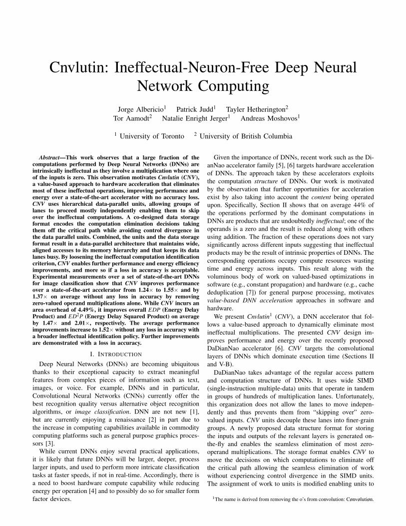
Fig. 1: Average fraction of convolutional layer multiplicationinput neuron values that are zero.

The key motivating observation for this work is that inpractice, many of the neuron values turn out to be zero,thus the corresponding multiplications and additions do notcontribute to the final result and could be avoided. Accord-ingly, this section characterizes the fraction of input neuronsthat are equal to zero in the convolutional layers of popularDNNs that are publicly available in Modelzoo [16]. For thesemeasurements the DNNs were used to classify one thousandof images from the Imagenet dataset [17]. Section V-A detailsthe networks and methodology followed.

Figure 1 reports the average total fraction of multiplicationoperands that are neuron inputs with a value of zero across allconvolutional layers and across all inputs. This fraction variesfrom 37% for nin, to up to 50% for cnnS and the averageacross all networks is 44%. The error bars show little variationacross input images, and given that the sample set of 1,000images is sizeable, the relatively large fraction of zero neuronsare due to the operation of the networks and not a property ofthe input.

But why would a network produce so many zero neurons?We hypothesize that the answer lies in the nature and structureof DNNs. At a high level, DNNs are designed so that eachDNN layer attempts to determine whether and where the inputcontains certain learned “features” such as lines, curves ormore elaborate constructs. The presence of a feature is encodedas a positive valued neuron output and the absence as a zero-valued neuron. It stands to reason that when features exist,most likely they will not appear all over the input, moreover,not all features will exist. DNNs detect the presence of featuresusing the convolutional layers to produce an output encodingthe likelihood that a feature exists at a particular position witha number. Negative values suggest that a feature is not present.Convolutional layers are immediately followed by a Rectifier,or ReLU layer which lets positive values pass through, butconverts any negative input to zero.

While there are many zero-valued neurons, their positiondepends on the input data values, and hence it will be chal-lenging for a static approach to eliminate the correspondingcomputations. In particular, there were no neurons that werealways zero across all inputs. Even, if it was possible to

2

Output

NeuronsNeurons Filter 1(0,0,0) (1,0,0) Filter 0

Applying filter 0 at (0,0,0) Applying filter 1 at (0,1,0)

Output

(a) (b) (c)x iy

NeuronsOutput

Filter/window

(0,1,0) (1,1,0)

xx

∑

∑

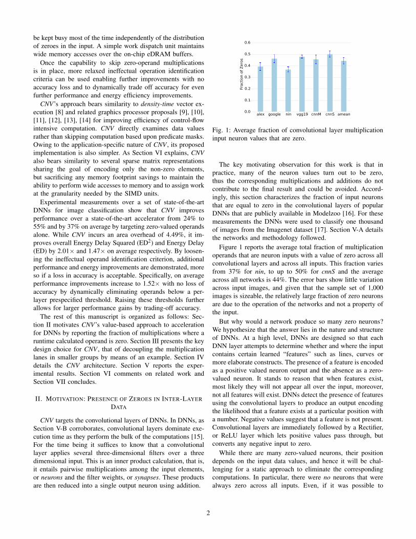
Fig. 2: The output neuron at position (0,0,0) or o(0,0,0) is produced by applying the filter on a 2×2×2 window of the inputwith origin n(0,0,0). Each synapse s(x,y,z) is multiplied by the corresponding input neuron n(x,y,z), e.g., n(0,0,0)×s(0,0,0),and n(0,1,0)× s(0,1,0), for a total of 2×2×2 or eight products. The eight products are reduced into a single output neuronusing addition. Then the window is slide over by S first along the X dimension to produce o(1,0,0) using the neuron inputwindow at origin n(1,0,0). For example, now s(0,0,0) is multiplied with n(1,0,0) and s(1,1,0) with n(2,1,0). Once the firstdimension is exhausted, then the window slides by S along the Y dimension and starts scanning along the X dimension again,and so on as the figure shows. In total, the result is a 2×2×1 output neuron. The depth is one since there is only one filter.Parts (b) and (c) show a convolutional layer with two 2× 2× 2 filters. The output now is a 2× 2× 2 array, with each filterproducing one of the two planes or layers of the output. As part (b) shows, the first filter produces output elements o(x,y,0).Part (c) shows that the second filter produces output neurons o(x,y,1).

eliminate neurons that were zero with high probability, therewould not be many. For example, only 0.6% of neurons arezero with 99% probability. Accordingly, this work proposesan architecture that detects and eliminates such computationsat runtime.

Since the time needed to compute a convolutional layerincreases mostly linearly with the number of elements pro-cessed and since convolutional layers dominate execution time,these measurements serve as an upper bound on the potentialperformance improvement for an architecture that manages toskip the computations corresponding to zero-valued neurons.

III. ENABLING ZERO SKIPPING:A SIMPLIFIED EXAMPLE

Having shown that many of the neurons are zero, thissection explains the two key ideas behind CNV that enable it toskip over the corresponding computations: 1) lane decoupling,and 2) storing the input on-the-fly in an appropriate format thatfacilitates the elimination of zero valued inputs. Section III-Afirst describes the computations that take place in a convolutionlayer identifying those that could be avoided when the inputneurons are zero. Since our goal is to improve upon the state-of-the-art, Section III-B describes a state-of-the-art acceleratorarchitecture for DNNs whose processing units couple severalgroups of processing lanes together into wide SIMD units.Finally, Section III-C describes a basic CNV architecturewhich decouples the processing lane groups enabling them toproceed independently from one another and thus to skip zero-valued neurons. A number of additional challenges arise oncethe lane groups start operating independently. These challengesalong with the solutions that result in a practical, simple CNVdesign are described in Section IV-B.

A. Computation of Convolutional Layers

The operations involved in computing a CNN are of thesame nature as in a DNN. The main difference is that in

the former, weights are repeated so as to look for a featureat different points in an input (i.e. an image). The inputto a convolutional layer is a 3D array of real numbers ofdimensions Ix × Iy × i. These numbers are the input data inthe first layer and the outputs of the neurons of the previouslayer for subsequent layers. In the remainder of this work, wewill call them input neurons. Each layer applies N filters atmultiple positions along x and y dimensions of the layer input.Each filter is a 3D array of dimensions Fx ×Fy × i containingsynapses. All filters are of equal dimensions and their depth isthe same as the input neuron array’s. The layer produces a 3Doutput neuron array of dimensions Ox ×Oy ×N. The output’sdepth is the same as the number of the filters.

To calculate an output neuron, one filter is applied overa window, or a subarray of the input neuron array that hasthe same dimensions as the filters Fx × Fy × i. Let n(x,y,z)and o(x,y,z) be respectively input and output neurons, ands f (x,y,z) be synapses of filter f . The output neuron at position(k, l,f), before the activation function, is calculated as follows:

o(k, l,f)︸ ︷︷ ︸out putneuron

=Fy−1

∑y=0

Fx−1

∑x=0

I−1

∑i=0

sf(y,x, i)︸ ︷︷ ︸synapse

×n(y+ l×S,x+k×S, i)︸ ︷︷ ︸input neuron︸ ︷︷ ︸

window

There is one output neuron per window and filter. The filtersare applied repeatedly over different windows moving alongthe X and Y dimensions using a constant stride S to produceall the output neurons. Accordingly, the output neuron arraydimensions are Ox = (Ix−Fx)/S+1, and Oy = (Iy−Fy)/S+1.Figure 2 shows a example with a 3×3×2 input neuron array,a single 2× 2× 2 filter and unit stride producing an outputneuron array of 2×2×1.

When an input neuron is zero the corresponding multipli-cation and addition can be eliminated to save time and energywithout altering the output value.

3

12

-1-2

0

4

04

2

(a) (b)

cycle 0 cycle 1 cycle 2

(c)

1 13 3

0

1 15 5

3

2 26 6

4Filter 0

-1 -1-5 -5

-3-2 -2-6 -6

-4

Filter 1

0 02

3 34

-3-4

3 34

5 56

-5

Input neurons

Filter 0 Filter 0

Filter 1 Filter 1

(d)

-3

-5-61 1

0

1 12

Filter 0

Filter 1

-1 -1-2

Output neurons

48-48

Input neurons

1 1-1

Corresp.Filter 1Corresp.

Filter 0

NBout

+5

SB3 1

6 4 2

-5 -3 -1

-6 -4 -2

3 0 1

4 2 0

x

x

x

x+

1-1

Filter 0 Lane

NBinNeuron Lane 0

NBinentry

Filter 1 Lane

Neuron Lane1

SBentry

Input neurons

NBout

+5SB

36 4

-5 -3-6 -4

3 0

4 2

xx

xx +

9-9

NBin

9 9-9 48

48

-48

Input neuronsOutput neurons

Output neurons

Outputneurons

34

-3-4

12

-1-2

NBout

+5SB

6

-5-6

3

4

xx

xx +

48-48

NBin

SynapseLane 0

SynapseLane 1

SynapseLane 0

SynapseLane 1

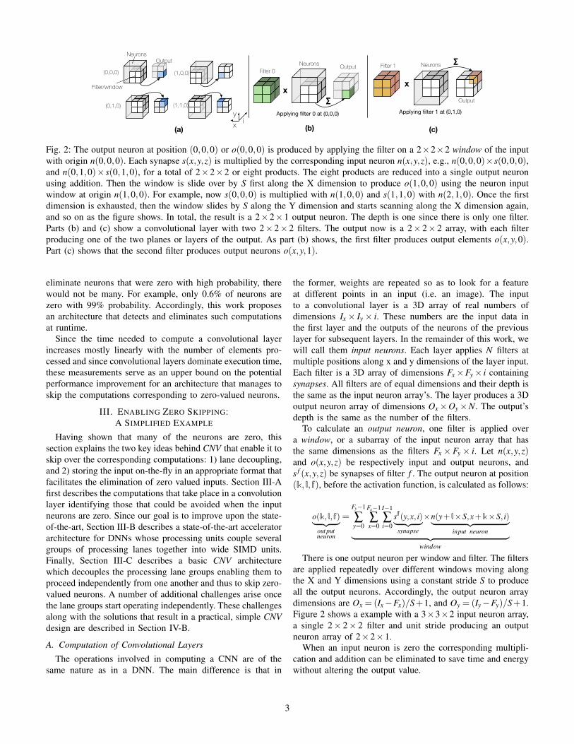
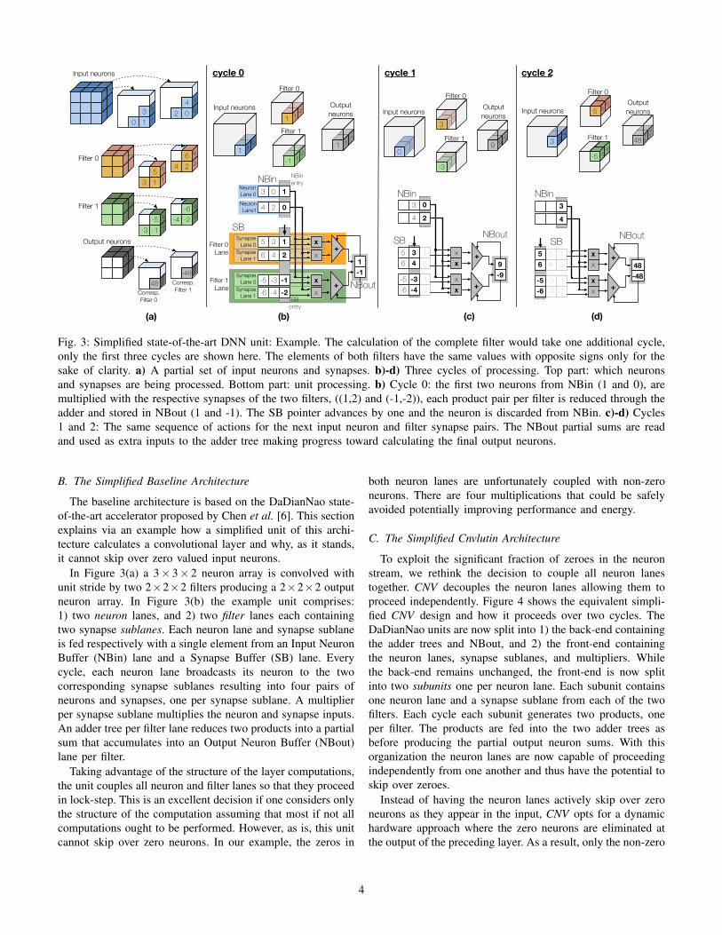
Fig. 3: Simplified state-of-the-art DNN unit: Example. The calculation of the complete filter would take one additional cycle,only the first three cycles are shown here. The elements of both filters have the same values with opposite signs only for thesake of clarity. a) A partial set of input neurons and synapses. b)-d) Three cycles of processing. Top part: which neuronsand synapses are being processed. Bottom part: unit processing. b) Cycle 0: the first two neurons from NBin (1 and 0), aremultiplied with the respective synapses of the two filters, ((1,2) and (-1,-2)), each product pair per filter is reduced through theadder and stored in NBout (1 and -1). The SB pointer advances by one and the neuron is discarded from NBin. c)-d) Cycles1 and 2: The same sequence of actions for the next input neuron and filter synapse pairs. The NBout partial sums are readand used as extra inputs to the adder tree making progress toward calculating the final output neurons.

B. The Simplified Baseline Architecture

The baseline architecture is based on the DaDianNao state-of-the-art accelerator proposed by Chen et al. [6]. This sectionexplains via an example how a simplified unit of this archi-tecture calculates a convolutional layer and why, as it stands,it cannot skip over zero valued input neurons.

In Figure 3(a) a 3× 3× 2 neuron array is convolved withunit stride by two 2×2×2 filters producing a 2×2×2 outputneuron array. In Figure 3(b) the example unit comprises:1) two neuron lanes, and 2) two filter lanes each containingtwo synapse sublanes. Each neuron lane and synapse sublaneis fed respectively with a single element from an Input NeuronBuffer (NBin) lane and a Synapse Buffer (SB) lane. Everycycle, each neuron lane broadcasts its neuron to the twocorresponding synapse sublanes resulting into four pairs ofneurons and synapses, one per synapse sublane. A multiplierper synapse sublane multiplies the neuron and synapse inputs.An adder tree per filter lane reduces two products into a partialsum that accumulates into an Output Neuron Buffer (NBout)lane per filter.

Taking advantage of the structure of the layer computations,the unit couples all neuron and filter lanes so that they proceedin lock-step. This is an excellent decision if one considers onlythe structure of the computation assuming that most if not allcomputations ought to be performed. However, as is, this unitcannot skip over zero neurons. In our example, the zeros in

both neuron lanes are unfortunately coupled with non-zeroneurons. There are four multiplications that could be safelyavoided potentially improving performance and energy.

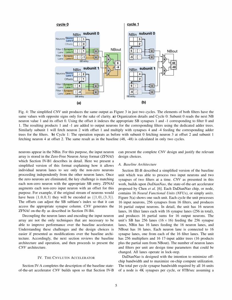
C. The Simplified Cnvlutin Architecture

To exploit the significant fraction of zeroes in the neuronstream, we rethink the decision to couple all neuron lanestogether. CNV decouples the neuron lanes allowing them toproceed independently. Figure 4 shows the equivalent simpli-fied CNV design and how it proceeds over two cycles. TheDaDianNao units are now split into 1) the back-end containingthe adder trees and NBout, and 2) the front-end containingthe neuron lanes, synapse sublanes, and multipliers. Whilethe back-end remains unchanged, the front-end is now splitinto two subunits one per neuron lane. Each subunit containsone neuron lane and a synapse sublane from each of the twofilters. Each cycle each subunit generates two products, oneper filter. The products are fed into the two adder trees asbefore producing the partial output neuron sums. With thisorganization the neuron lanes are now capable of proceedingindependently from one another and thus have the potential toskip over zeroes.

Instead of having the neuron lanes actively skip over zeroneurons as they appear in the input, CNV opts for a dynamichardware approach where the zero neurons are eliminated atthe output of the preceding layer. As a result, only the non-zero

4

NBout

SynapseLane 1

SynapseLane 1

2 1Offsets

6 4 2

-6 -4 -2

4 2

x

x

9-9

Filter 0Lane

(a)

subunit 0NBin

cycle 0

+

Filter 1Lane

Neuron Lane 1

SynapseLane 0

SynapseLane 0

2 0Offsets

5 3 1

-5 -3 -1

3 1

x

x

Filter 0Lane

Filter 1Lane

Neuron Lane 0

+

SB entry

SB entry

subunit 1NBin

2

6 4 2

-6 -4 -2

4

x

x

48-48

(b)

subunit 0NBin

cycle 1

+

2

5 3 1

-5 -3 -1

3

x

x

+

SB entry

subunit 1NBinNeurons

Neurons

NBout

Fig. 4: The simplified CNV unit produces the same output as Figure 3 in just two cycles. The elements of both filters have thesame values with opposite signs only for the sake of clarity. a) Organization details and Cycle 0: Subunit 0 reads the next NBneuron value 1 and its offset 0. Using the offset it indexes the appropriate SB synapses 1 and -1 corresponding to filter 0 and1. The resulting products 1 and -1 are added to output neurons for the corresponding filters using the dedicated adder trees.Similarly subunit 1 will fetch neuron 2 with offset 1 and multiply with synapses 4 and -4 feeding the corresponding addertrees for the filters. b) Cycle 1: The operation repeats as before with subunit 0 fetching neuron 3 at offset 2 and subunit 1fetching neuron 4 at offset 2. The same result as in the baseline (48, -48) is calculated in only two cycles.

neurons appear in the NBin. For this purpose, the input neuronarray is stored in the Zero-Free Neuron Array format (ZFNAf)which Section IV-B1 describes in detail. Here we present asimplified version of this format explaining how it allowsindividual neuron lanes to see only the non-zero neuronsproceeding independently from the other neuron lanes. Oncethe zero neurons are eliminated, the key challenge is matchingeach non-zero neuron with the appropriate SB entry. ZFNAfaugments each non-zero input neuron with an offset for thispurpose. For example, if the original stream of neurons wouldhave been (1,0,0,3) they will be encoded as ((1,0),(3,3)).The offsets can adjust the SB sublane’s index so that it canaccess the appropriate synapse column. CNV generates theZFNAf on-the-fly as described in Section IV-B4.

Decoupling the neuron lanes and encoding the input neuronarray are not the only techniques that are necessary to beable to improve performance over the baseline accelerator.Understanding these challenges and the design choices iseasier if presented as modifications over the baseline archi-tecture. Accordingly, the next section reviews the baselinearchitecture and operation, and then proceeds to present theCNV architecture.

IV. THE CNVLUTIN ACCELERATOR

Section IV-A completes the description of the baseline state-of-the-art accelerator CNV builds upon so that Section IV-B

can present the complete CNV design and justify the relevantdesign choices.

A. Baseline Architecture

Section III-B described a simplified version of the baselineunit which was able to process two input neurons and twosynapses of two filters at a time. CNV as presented in thiswork, builds upon DaDianNao, the state-of-the-art acceleratorproposed by Chen et al. [6]. Each DaDianNao chip, or node,contains 16 Neural Functional Units (NFUs), or simply units.Figure 5(a) shows one such unit. Each cycle the unit processes16 input neurons, 256 synapses from 16 filters, and produces16 partial output neurons. In detail, the unit has 16 neuronlanes, 16 filter lanes each with 16 synapse lanes (256 in total),and produces 16 partial sums for 16 output neurons. Theunit’s SB has 256 lanes (16× 16) feeding the 256 synapselanes, NBin has 16 lanes feeding the 16 neuron lanes, andNBout has 16 lanes. Each neuron lane is connected to 16synapse lanes, one from each of the 16 filter lanes. The unithas 256 multipliers and 16 17-input adder trees (16 productsplus the partial sum from NBout). The number of neuron lanesand filters per unit are design time parameters that could bechanged. All lanes operate in lock-step.

DaDianNao is designed with the intention to minimize off-chip bandwidth and to maximize on-chip compute utilization.The total per cycle synapse bandwidth required by all 16 unitsof a node is 4K synapses per cycle, or 8TB/sec assuming a

5

SB (e

DRAM

) SynapseLane 15

SynapseLane 15

Lane 0Filter

Lane 15Filter

SynapseLane 0

SynapseLane 15

SB (eDRAM)

NBin

x

xf

NBout+Filter

Lane 0

FilterLane 15

x

x+ f

64

from central eDRAM

to central eDRAM

x

x

Offsets

Subunit 0

64

+

NBout

to centraleDRAM

SB (e

DRAM

)

encoder

f

+ f

x

x

Subunit 15

64

from centraleDRAM

from centraleDRAM

Nbin

SynapseLane 0

SynapseLane 15

NeuronLane 0

NeuronLane 15

NeuronLane 0

64

64

NeuronLane 15

Offsets

SynapseLane 0

SynapseLane 0

Lane 0Filter

Nbin

Lane 15Filter

64

(a) (b)

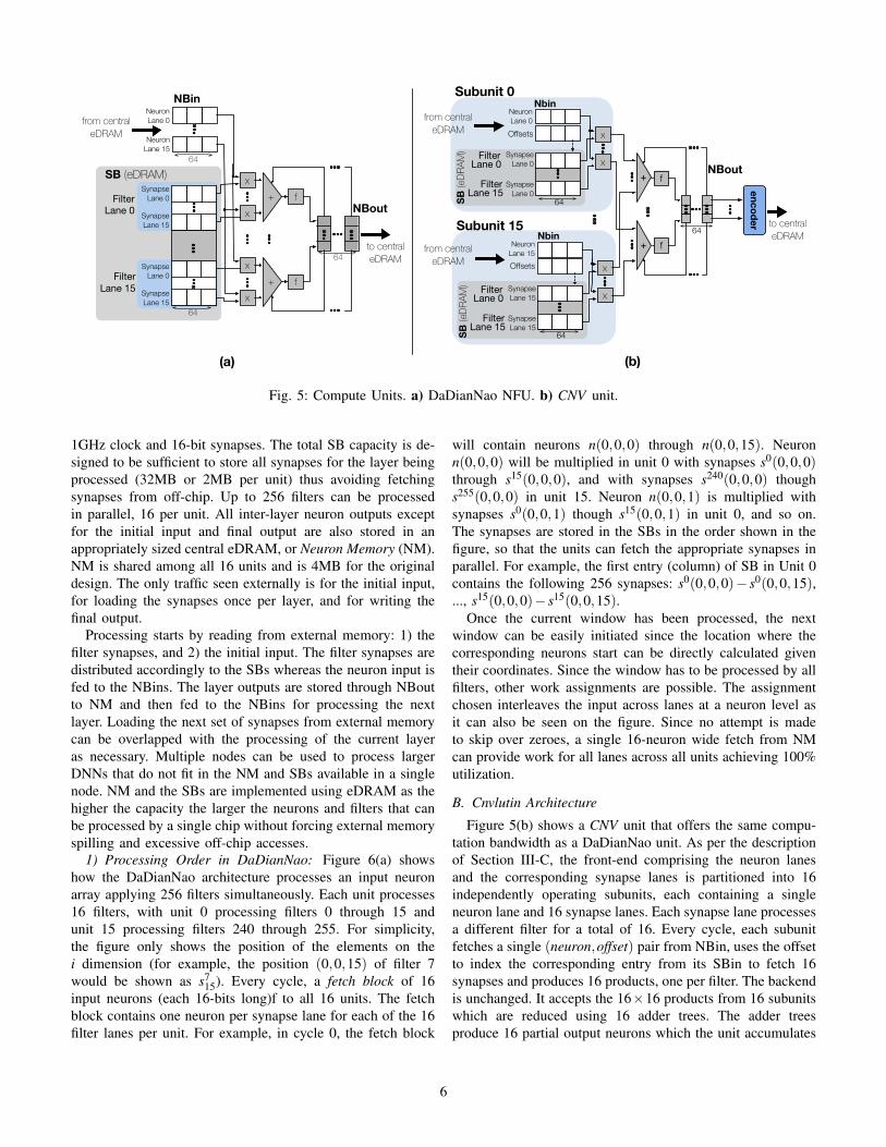
Fig. 5: Compute Units. a) DaDianNao NFU. b) CNV unit.

1GHz clock and 16-bit synapses. The total SB capacity is de-signed to be sufficient to store all synapses for the layer beingprocessed (32MB or 2MB per unit) thus avoiding fetchingsynapses from off-chip. Up to 256 filters can be processedin parallel, 16 per unit. All inter-layer neuron outputs exceptfor the initial input and final output are also stored in anappropriately sized central eDRAM, or Neuron Memory (NM).NM is shared among all 16 units and is 4MB for the originaldesign. The only traffic seen externally is for the initial input,for loading the synapses once per layer, and for writing thefinal output.

Processing starts by reading from external memory: 1) thefilter synapses, and 2) the initial input. The filter synapses aredistributed accordingly to the SBs whereas the neuron input isfed to the NBins. The layer outputs are stored through NBoutto NM and then fed to the NBins for processing the nextlayer. Loading the next set of synapses from external memorycan be overlapped with the processing of the current layeras necessary. Multiple nodes can be used to process largerDNNs that do not fit in the NM and SBs available in a singlenode. NM and the SBs are implemented using eDRAM as thehigher the capacity the larger the neurons and filters that canbe processed by a single chip without forcing external memoryspilling and excessive off-chip accesses.

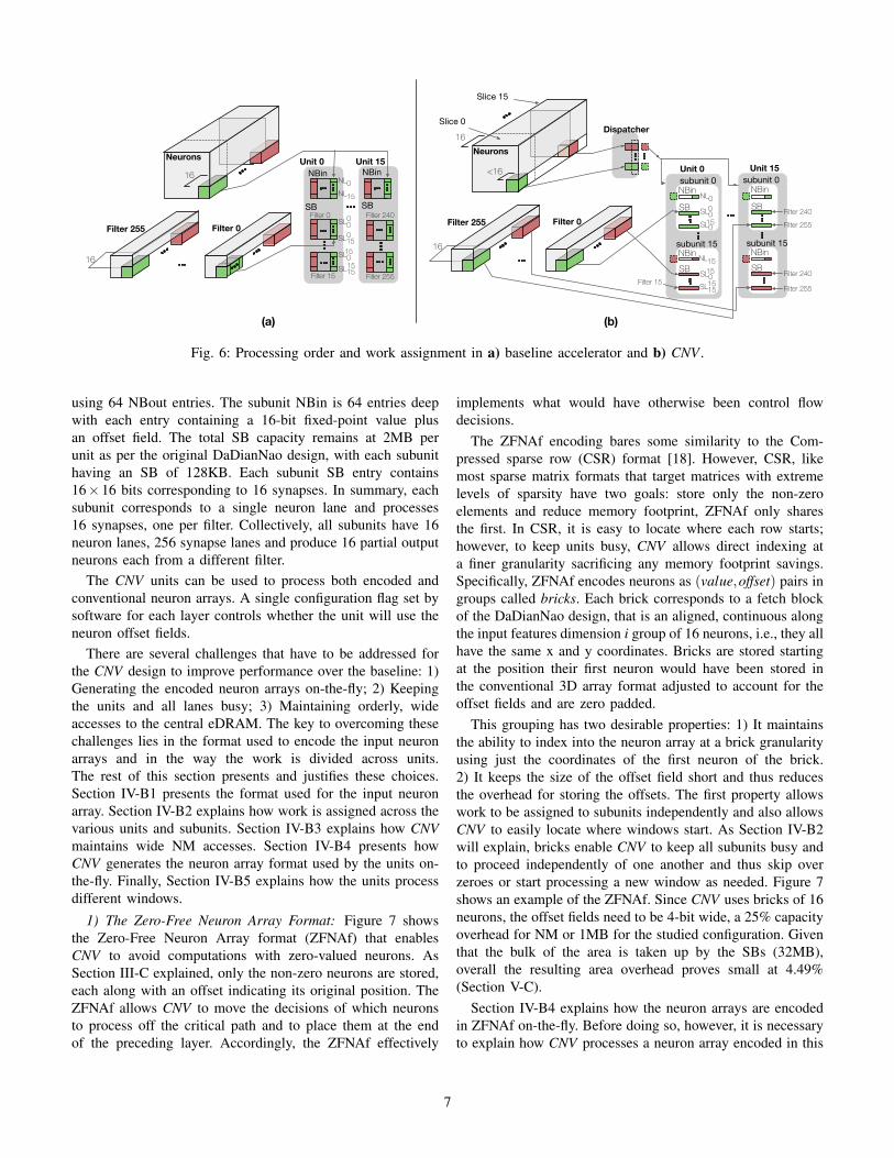
1) Processing Order in DaDianNao: Figure 6(a) showshow the DaDianNao architecture processes an input neuronarray applying 256 filters simultaneously. Each unit processes16 filters, with unit 0 processing filters 0 through 15 andunit 15 processing filters 240 through 255. For simplicity,the figure only shows the position of the elements on thei dimension (for example, the position (0,0,15) of filter 7would be shown as s7

15). Every cycle, a fetch block of 16input neurons (each 16-bits long)f to all 16 units. The fetchblock contains one neuron per synapse lane for each of the 16filter lanes per unit. For example, in cycle 0, the fetch block

will contain neurons n(0,0,0) through n(0,0,15). Neuronn(0,0,0) will be multiplied in unit 0 with synapses s0(0,0,0)through s15(0,0,0), and with synapses s240(0,0,0) thoughs255(0,0,0) in unit 15. Neuron n(0,0,1) is multiplied withsynapses s0(0,0,1) though s15(0,0,1) in unit 0, and so on.The synapses are stored in the SBs in the order shown in thefigure, so that the units can fetch the appropriate synapses inparallel. For example, the first entry (column) of SB in Unit 0contains the following 256 synapses: s0(0,0,0)− s0(0,0,15),..., s15(0,0,0)− s15(0,0,15).

Once the current window has been processed, the nextwindow can be easily initiated since the location where thecorresponding neurons start can be directly calculated giventheir coordinates. Since the window has to be processed by allfilters, other work assignments are possible. The assignmentchosen interleaves the input across lanes at a neuron level asit can also be seen on the figure. Since no attempt is madeto skip over zeroes, a single 16-neuron wide fetch from NMcan provide work for all lanes across all units achieving 100%utilization.

B. Cnvlutin Architecture

Figure 5(b) shows a CNV unit that offers the same compu-tation bandwidth as a DaDianNao unit. As per the descriptionof Section III-C, the front-end comprising the neuron lanesand the corresponding synapse lanes is partitioned into 16independently operating subunits, each containing a singleneuron lane and 16 synapse lanes. Each synapse lane processesa different filter for a total of 16. Every cycle, each subunitfetches a single (neuron,offset) pair from NBin, uses the offsetto index the corresponding entry from its SBin to fetch 16synapses and produces 16 products, one per filter. The backendis unchanged. It accepts the 16×16 products from 16 subunitswhich are reduced using 16 adder trees. The adder treesproduce 16 partial output neurons which the unit accumulates

6

(a) (b)

NBinUnit 0

Filter 0SB

NBinUnit 15

Filter 15

Filter 0Filter 255Filter 240

SB

Filter 255

Neurons16

NL0NL15

SL00

SL150

SL015

SL1515

16

Unit 0

SB

NL0

subunit 0

SB

NBin

NL15

SL00

SL015

SL015

SL1515

NBinsubunit 15

Unit 15

SB

subunit 0

SB

NBin

NBinsubunit 15

Filter 0Filter 255

16

DispatcherSlice 0

Filter 15Filter 240

Filter 240

<16

Filter 255

Filter 255

Neurons

16

Slice 15

Fig. 6: Processing order and work assignment in a) baseline accelerator and b) CNV .

using 64 NBout entries. The subunit NBin is 64 entries deepwith each entry containing a 16-bit fixed-point value plusan offset field. The total SB capacity remains at 2MB perunit as per the original DaDianNao design, with each subunithaving an SB of 128KB. Each subunit SB entry contains16×16 bits corresponding to 16 synapses. In summary, eachsubunit corresponds to a single neuron lane and processes16 synapses, one per filter. Collectively, all subunits have 16neuron lanes, 256 synapse lanes and produce 16 partial outputneurons each from a different filter.

The CNV units can be used to process both encoded andconventional neuron arrays. A single configuration flag set bysoftware for each layer controls whether the unit will use theneuron offset fields.

There are several challenges that have to be addressed forthe CNV design to improve performance over the baseline: 1)Generating the encoded neuron arrays on-the-fly; 2) Keepingthe units and all lanes busy; 3) Maintaining orderly, wideaccesses to the central eDRAM. The key to overcoming thesechallenges lies in the format used to encode the input neuronarrays and in the way the work is divided across units.The rest of this section presents and justifies these choices.Section IV-B1 presents the format used for the input neuronarray. Section IV-B2 explains how work is assigned across thevarious units and subunits. Section IV-B3 explains how CNVmaintains wide NM accesses. Section IV-B4 presents howCNV generates the neuron array format used by the units on-the-fly. Finally, Section IV-B5 explains how the units processdifferent windows.

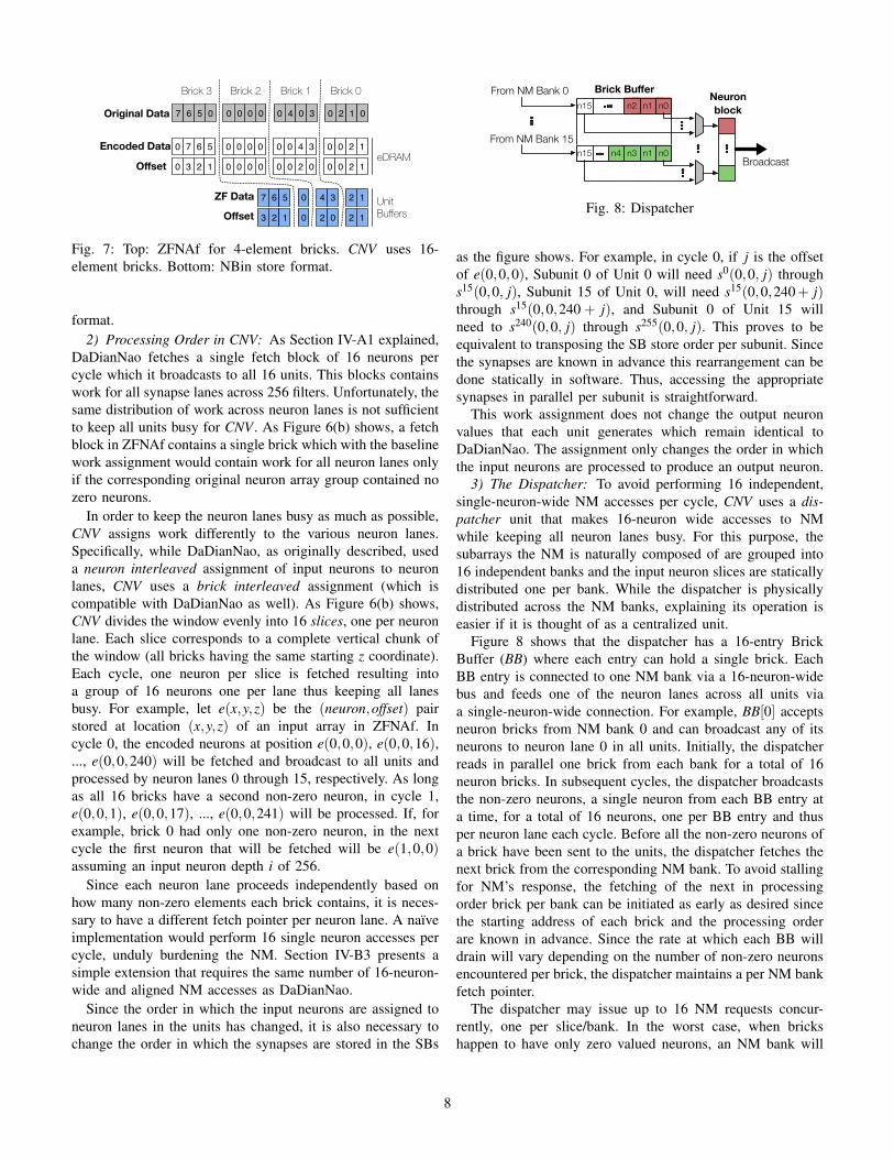
1) The Zero-Free Neuron Array Format: Figure 7 showsthe Zero-Free Neuron Array format (ZFNAf) that enablesCNV to avoid computations with zero-valued neurons. AsSection III-C explained, only the non-zero neurons are stored,each along with an offset indicating its original position. TheZFNAf allows CNV to move the decisions of which neuronsto process off the critical path and to place them at the endof the preceding layer. Accordingly, the ZFNAf effectively

implements what would have otherwise been control flowdecisions.

The ZFNAf encoding bares some similarity to the Com-pressed sparse row (CSR) format [18]. However, CSR, likemost sparse matrix formats that target matrices with extremelevels of sparsity have two goals: store only the non-zeroelements and reduce memory footprint, ZFNAf only sharesthe first. In CSR, it is easy to locate where each row starts;however, to keep units busy, CNV allows direct indexing ata finer granularity sacrificing any memory footprint savings.Specifically, ZFNAf encodes neurons as (value,offset) pairs ingroups called bricks. Each brick corresponds to a fetch blockof the DaDianNao design, that is an aligned, continuous alongthe input features dimension i group of 16 neurons, i.e., they allhave the same x and y coordinates. Bricks are stored startingat the position their first neuron would have been stored inthe conventional 3D array format adjusted to account for theoffset fields and are zero padded.

This grouping has two desirable properties: 1) It maintainsthe ability to index into the neuron array at a brick granularityusing just the coordinates of the first neuron of the brick.2) It keeps the size of the offset field short and thus reducesthe overhead for storing the offsets. The first property allowswork to be assigned to subunits independently and also allowsCNV to easily locate where windows start. As Section IV-B2will explain, bricks enable CNV to keep all subunits busy andto proceed independently of one another and thus skip overzeroes or start processing a new window as needed. Figure 7shows an example of the ZFNAf. Since CNV uses bricks of 16neurons, the offset fields need to be 4-bit wide, a 25% capacityoverhead for NM or 1MB for the studied configuration. Giventhat the bulk of the area is taken up by the SBs (32MB),overall the resulting area overhead proves small at 4.49%(Section V-C).

Section IV-B4 explains how the neuron arrays are encodedin ZFNAf on-the-fly. Before doing so, however, it is necessaryto explain how CNV processes a neuron array encoded in this

7

7

Brick 0

Original Data

Encoded Data

Offset

6 5 0 0 0 0 0 0 4 0 3 0 2 1 0

0 7 6 5 0 0 0 0 0 0 4 3 0 0 2 1

0 3 2 1 0 0 0 0 0 0 2 0 0 0 2 1

7 6 5 0 4 3 2 1

3 2 1 0 2 0 2 1

ZF Data

Brick 1Brick 2Brick 3

Offset

eDRAM

UnitBuffers

Fig. 7: Top: ZFNAf for 4-element bricks. CNV uses 16-element bricks. Bottom: NBin store format.

format.2) Processing Order in CNV: As Section IV-A1 explained,

DaDianNao fetches a single fetch block of 16 neurons percycle which it broadcasts to all 16 units. This blocks containswork for all synapse lanes across 256 filters. Unfortunately, thesame distribution of work across neuron lanes is not sufficientto keep all units busy for CNV . As Figure 6(b) shows, a fetchblock in ZFNAf contains a single brick which with the baselinework assignment would contain work for all neuron lanes onlyif the corresponding original neuron array group contained nozero neurons.

In order to keep the neuron lanes busy as much as possible,CNV assigns work differently to the various neuron lanes.Specifically, while DaDianNao, as originally described, useda neuron interleaved assignment of input neurons to neuronlanes, CNV uses a brick interleaved assignment (which iscompatible with DaDianNao as well). As Figure 6(b) shows,CNV divides the window evenly into 16 slices, one per neuronlane. Each slice corresponds to a complete vertical chunk ofthe window (all bricks having the same starting z coordinate).Each cycle, one neuron per slice is fetched resulting intoa group of 16 neurons one per lane thus keeping all lanesbusy. For example, let e(x,y,z) be the (neuron,offset) pairstored at location (x,y,z) of an input array in ZFNAf. Incycle 0, the encoded neurons at position e(0,0,0), e(0,0,16),..., e(0,0,240) will be fetched and broadcast to all units andprocessed by neuron lanes 0 through 15, respectively. As longas all 16 bricks have a second non-zero neuron, in cycle 1,e(0,0,1), e(0,0,17), ..., e(0,0,241) will be processed. If, forexample, brick 0 had only one non-zero neuron, in the nextcycle the first neuron that will be fetched will be e(1,0,0)assuming an input neuron depth i of 256.

Since each neuron lane proceeds independently based onhow many non-zero elements each brick contains, it is neces-sary to have a different fetch pointer per neuron lane. A naıveimplementation would perform 16 single neuron accesses percycle, unduly burdening the NM. Section IV-B3 presents asimple extension that requires the same number of 16-neuron-wide and aligned NM accesses as DaDianNao.

Since the order in which the input neurons are assigned toneuron lanes in the units has changed, it is also necessary tochange the order in which the synapses are stored in the SBs

n15

n1n2 n0

n4 n0

Brick BufferFrom NM Bank 0

From NM Bank 15

Neuronblock

Broadcast

n15

n3 n1

Fig. 8: Dispatcher

as the figure shows. For example, in cycle 0, if j is the offsetof e(0,0,0), Subunit 0 of Unit 0 will need s0(0,0, j) throughs15(0,0, j), Subunit 15 of Unit 0, will need s15(0,0,240+ j)through s15(0,0,240 + j), and Subunit 0 of Unit 15 willneed to s240(0,0, j) through s255(0,0, j). This proves to beequivalent to transposing the SB store order per subunit. Sincethe synapses are known in advance this rearrangement can bedone statically in software. Thus, accessing the appropriatesynapses in parallel per subunit is straightforward.

This work assignment does not change the output neuronvalues that each unit generates which remain identical toDaDianNao. The assignment only changes the order in whichthe input neurons are processed to produce an output neuron.

3) The Dispatcher: To avoid performing 16 independent,single-neuron-wide NM accesses per cycle, CNV uses a dis-patcher unit that makes 16-neuron wide accesses to NMwhile keeping all neuron lanes busy. For this purpose, thesubarrays the NM is naturally composed of are grouped into16 independent banks and the input neuron slices are staticallydistributed one per bank. While the dispatcher is physicallydistributed across the NM banks, explaining its operation iseasier if it is thought of as a centralized unit.

Figure 8 shows that the dispatcher has a 16-entry BrickBuffer (BB) where each entry can hold a single brick. EachBB entry is connected to one NM bank via a 16-neuron-widebus and feeds one of the neuron lanes across all units viaa single-neuron-wide connection. For example, BB[0] acceptsneuron bricks from NM bank 0 and can broadcast any of itsneurons to neuron lane 0 in all units. Initially, the dispatcherreads in parallel one brick from each bank for a total of 16neuron bricks. In subsequent cycles, the dispatcher broadcaststhe non-zero neurons, a single neuron from each BB entry ata time, for a total of 16 neurons, one per BB entry and thusper neuron lane each cycle. Before all the non-zero neurons ofa brick have been sent to the units, the dispatcher fetches thenext brick from the corresponding NM bank. To avoid stallingfor NM’s response, the fetching of the next in processingorder brick per bank can be initiated as early as desired sincethe starting address of each brick and the processing orderare known in advance. Since the rate at which each BB willdrain will vary depending on the number of non-zero neuronsencountered per brick, the dispatcher maintains a per NM bankfetch pointer.

The dispatcher may issue up to 16 NM requests concur-rently, one per slice/bank. In the worst case, when brickshappen to have only zero valued neurons, an NM bank will

8

have to supply a new brick every cycle. This rarely happensin practice, and the NM banks are relatively large and aresub-banked to sustain this worst case bandwidth.

In DaDianNao, a single 16-neuron wide interconnect is usedto broadcast the fetch block to all 16 units. The interconnectstructure remains unchanged in CNV but the width increasesto accommodate the neuron offsets.

4) Generating the ZFNAf: The initial input to the DNNsstudied are images which are processed using a conventional3D array format. The first layer treats them as a 3-feature deepneuron array with each color plane being a feature. All otherconvolutional layers use the ZFNAf which CNV generates on-the-fly at the output of the immediately preceding layer.

In CNV as in DaDianNao, output neurons are written to NMfrom NBout before they can be fed as input to another layer.Since the eDRAM NM favors wide accesses, these writesremain 16 neurons wide. However, before writing to the NM,each 16-neuron group is encoded into a brick in ZFNAf. Thisis done by the Encoder subunit. One encoder subunit existsper CNV unit.

While CNV processes the input neuron array in an orderdifferent than DaDianNao, CNV’s units still produce the sameoutput neurons as DaDianNao. Recall, that each output neuronis produced by processing a whole window using one filter.The assignments of filters to units remain the same in CNV .Accordingly, the output neurons produced by a CNV unitcorrespond to a brick of the output neuron array. All theencoder unit has to do, is pack the non-zero neurons withinthe brick.

The Encoder uses a 16-neuron input buffer (IB), a 16-encoded-neuron output buffer (OB), and an offset counter.Conversion begins by reading a 16-neuron entry from NBoutinto IB while clearing all OB entries. Every cycle the encoderreads the next neuron from IB and increments its offsetcounter. The neuron is copied to the next OB position only ifit is nonzero. The current value of the offset counter is alsowritten completing the encoded neuron pair. Once all 16 IBneurons have been processed, the OB contains the brick inZFNMf and can be sent to NM. The same interconnect as inDaDianNao is used widened to accommodate the offset fields.The encoder can afford to do the encoding serially since: 1)output neurons are produced at a much slower rate, and 2) theencoded brick is needed for the next layer.

5) Synchronization: In DaDianNao, all units process neu-rons from the same window and processing the next windowproceeds only after the current window is processed. CNVfollows this approach avoiding further modifications to theunit’s back-end and control. As neuron lanes process theirbricks independently, unless all slices have exactly the samenumber of non-zero neurons, some neuron lanes will finishprocessing their window slice earlier than others. These neuronlanes will remain idle until all other lanes complete theirprocessing.

Network Conv.Layers Source

alex 5 Caffe: bvlc reference caffenetgoogle 59 Caffe: bvlc googlenetnin 12 Model Zoo: NIN-imagenetvgg19 16 Model Zoo: VGG 19-layercnnM 5 Model Zoo: VGG CNN M 2048cnnS 5 Model Zoo: VGG CNN S

TABLE I: Networks used

V. EVALUATION

This section evaluates the performance, area and power ofthe CNV architecture demonstrating how it improves overthe state-of-the-art DaDianNao accelerator [6]. Section V-Adetails the experimental methodology. Section V-B evaluatesthe performance of CNV . Sections V-C and V-D evaluatethe area and power of CNV , and Section V-E considers theremoval of non-zero neurons.

A. Methodology

The evaluation uses the set of popular [3], and state-of-the-art convolutional neural networks [19][16][20][21] shownin Table I. These networks perform image classification onthe ILSVRC12 dataset [19], which contains 256×256 imagesacross 1000 classes. The experiments use a randomly selectedset of 1000 images, one from each class. The networks areavailable, pre-trained for Caffe, either as part of the distributionor at the Caffe Model Zoo [22].

We created a cycle accurate simulator of the baselineaccelerator and CNV . The simulator integrates with the Caffeframework [23] to enable on-the-fly validation of the layerouput neurons. The area and power characteristics of CNV andDaDianNao are measured with synthesized implementations.The two designs are implemented in Verilog and synthesizedvia the Synopsis Design Compiler [24] with the TSMC 65nmlibrary. The NBin, NBout, and CNV offset SRAM buffers weremodeled using the Artisan single-ported register file memorycompiler [25] using double-pumping to allow a read and writeper cycle. The eDRAM area and energy was modeled withDestiny [26].

B. Performance

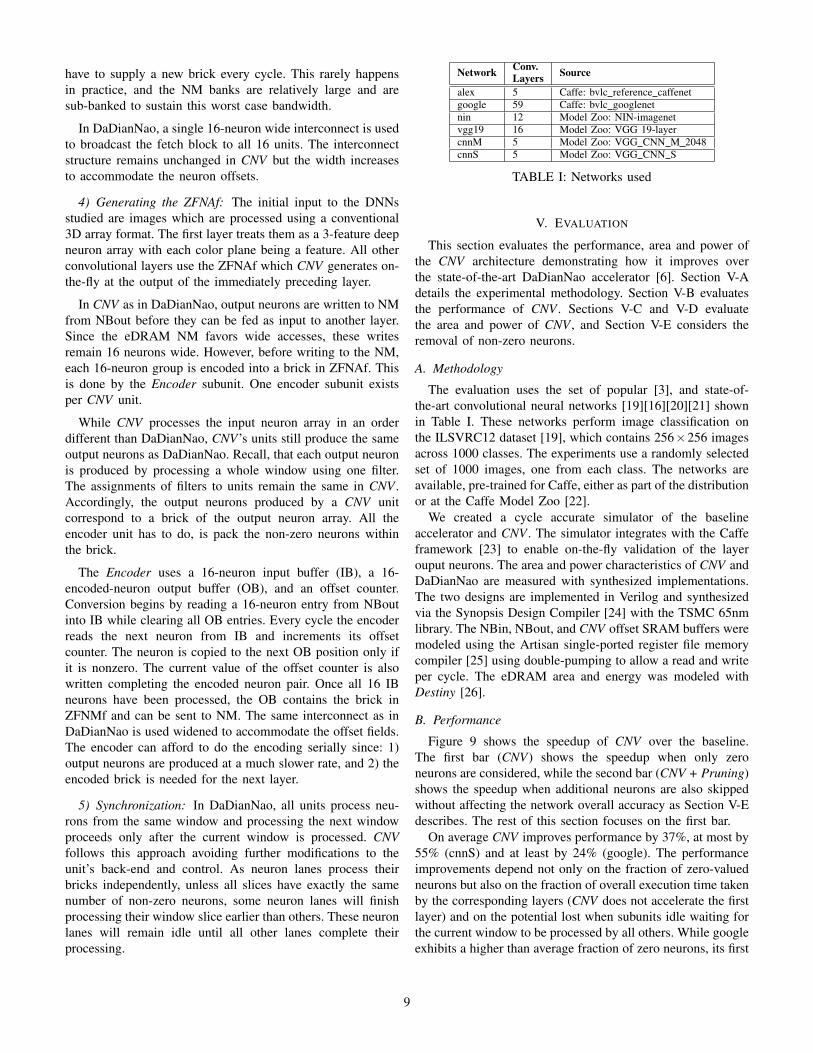
Figure 9 shows the speedup of CNV over the baseline.The first bar (CNV) shows the speedup when only zeroneurons are considered, while the second bar (CNV + Pruning)shows the speedup when additional neurons are also skippedwithout affecting the network overall accuracy as Section V-Edescribes. The rest of this section focuses on the first bar.

On average CNV improves performance by 37%, at most by55% (cnnS) and at least by 24% (google). The performanceimprovements depend not only on the fraction of zero-valuedneurons but also on the fraction of overall execution time takenby the corresponding layers (CNV does not accelerate the firstlayer) and on the potential lost when subunits idle waiting forthe current window to be processed by all others. While googleexhibits a higher than average fraction of zero neurons, its first

9

alex google nin vgg19 cnnM cnnS geo1.0

1.1

1.2

1.3

1.4

1.5

1.6

1.7

1.8

Speedup

CNV CNV + Pruning

Fig. 9: Speedup of CNV over the baseline.

layer has a relatively longer runtime than the other networksaccounting for 35% of the total runtime vs. 21% on average asmeasured on the baseline. Google also spends a higher portionof its timing computing other layers.

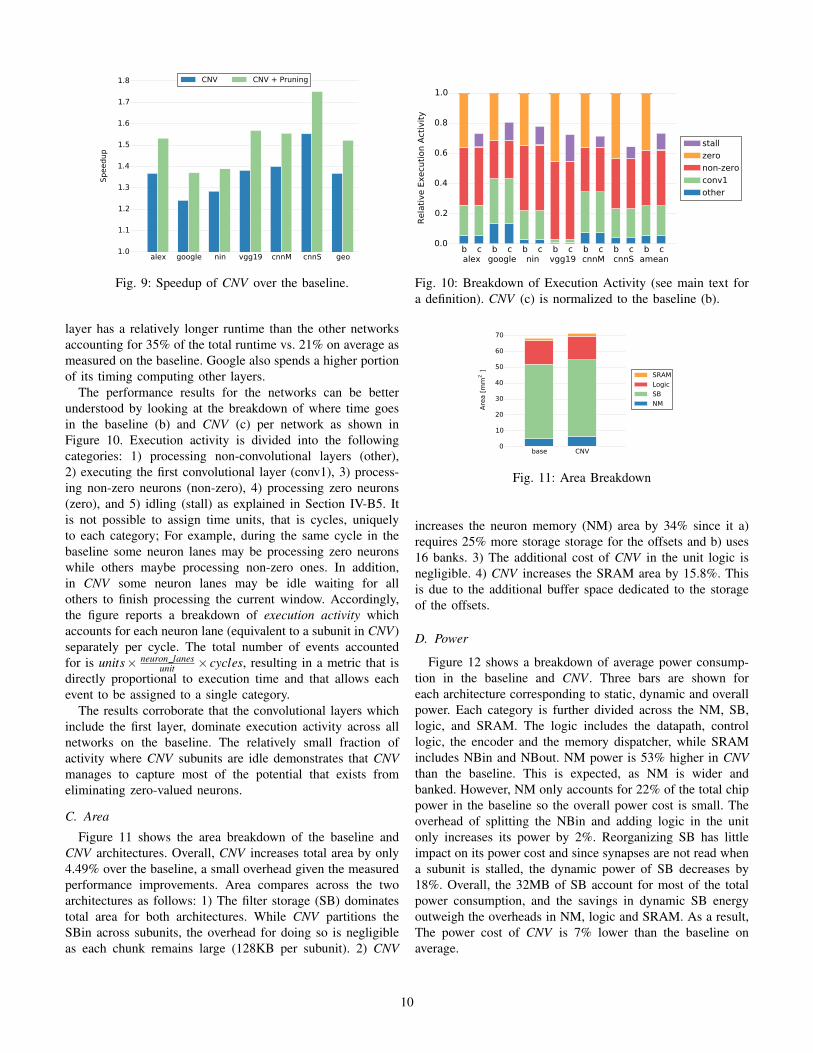
The performance results for the networks can be betterunderstood by looking at the breakdown of where time goesin the baseline (b) and CNV (c) per network as shown inFigure 10. Execution activity is divided into the followingcategories: 1) processing non-convolutional layers (other),2) executing the first convolutional layer (conv1), 3) process-ing non-zero neurons (non-zero), 4) processing zero neurons(zero), and 5) idling (stall) as explained in Section IV-B5. Itis not possible to assign time units, that is cycles, uniquelyto each category; For example, during the same cycle in thebaseline some neuron lanes may be processing zero neuronswhile others maybe processing non-zero ones. In addition,in CNV some neuron lanes may be idle waiting for allothers to finish processing the current window. Accordingly,the figure reports a breakdown of execution activity whichaccounts for each neuron lane (equivalent to a subunit in CNV)separately per cycle. The total number of events accountedfor is units× neuron lanes

unit × cycles, resulting in a metric that isdirectly proportional to execution time and that allows eachevent to be assigned to a single category.

The results corroborate that the convolutional layers whichinclude the first layer, dominate execution activity across allnetworks on the baseline. The relatively small fraction ofactivity where CNV subunits are idle demonstrates that CNVmanages to capture most of the potential that exists fromeliminating zero-valued neurons.

C. Area

Figure 11 shows the area breakdown of the baseline andCNV architectures. Overall, CNV increases total area by only4.49% over the baseline, a small overhead given the measuredperformance improvements. Area compares across the twoarchitectures as follows: 1) The filter storage (SB) dominatestotal area for both architectures. While CNV partitions theSBin across subunits, the overhead for doing so is negligibleas each chunk remains large (128KB per subunit). 2) CNV

b c b c b c b c b c b c b c0.0

0.2

0.4

0.6

0.8

1.0

Rela

tive E

xecu

tion A

ctiv

ity

alex google nin vgg19 cnnM cnnS amean

stall

zero

non-zero

conv1

other

Fig. 10: Breakdown of Execution Activity (see main text fora definition). CNV (c) is normalized to the baseline (b).

base CNV0

10

20

30

40

50

60

70

Are

a [

mm

2]

SRAM

Logic

SB

NM

Fig. 11: Area Breakdown

increases the neuron memory (NM) area by 34% since it a)requires 25% more storage storage for the offsets and b) uses16 banks. 3) The additional cost of CNV in the unit logic isnegligible. 4) CNV increases the SRAM area by 15.8%. Thisis due to the additional buffer space dedicated to the storageof the offsets.

D. Power

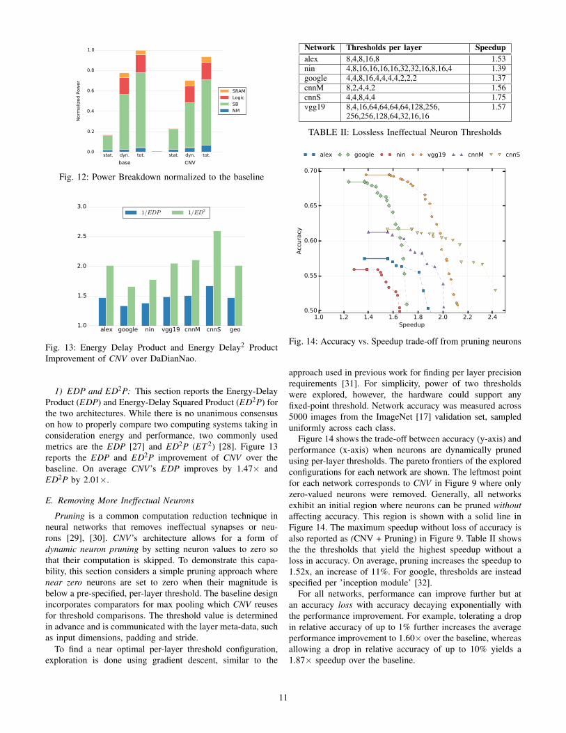
Figure 12 shows a breakdown of average power consump-tion in the baseline and CNV . Three bars are shown foreach architecture corresponding to static, dynamic and overallpower. Each category is further divided across the NM, SB,logic, and SRAM. The logic includes the datapath, controllogic, the encoder and the memory dispatcher, while SRAMincludes NBin and NBout. NM power is 53% higher in CNVthan the baseline. This is expected, as NM is wider andbanked. However, NM only accounts for 22% of the total chippower in the baseline so the overall power cost is small. Theoverhead of splitting the NBin and adding logic in the unitonly increases its power by 2%. Reorganizing SB has littleimpact on its power cost and since synapses are not read whena subunit is stalled, the dynamic power of SB decreases by18%. Overall, the 32MB of SB account for most of the totalpower consumption, and the savings in dynamic SB energyoutweigh the overheads in NM, logic and SRAM. As a result,The power cost of CNV is 7% lower than the baseline onaverage.

10

stat. dyn. tot. stat. dyn. tot.0.0

0.2

0.4

0.6

0.8

1.0

Norm

aliz

ed P

ow

er

base CNV

SRAM

Logic

SB

NM

Fig. 12: Power Breakdown normalized to the baseline

alex google nin vgg19 cnnM cnnS geo1.0

1.5

2.0

2.5

3.01/EDP 1/ED2

Fig. 13: Energy Delay Product and Energy Delay2 ProductImprovement of CNV over DaDianNao.

1) EDP and ED2P: This section reports the Energy-DelayProduct (EDP) and Energy-Delay Squared Product (ED2P) forthe two architectures. While there is no unanimous consensuson how to properly compare two computing systems taking inconsideration energy and performance, two commonly usedmetrics are the EDP [27] and ED2P (ET 2) [28]. Figure 13reports the EDP and ED2P improvement of CNV over thebaseline. On average CNV’s EDP improves by 1.47× andED2P by 2.01×.

E. Removing More Ineffectual Neurons

Pruning is a common computation reduction technique inneural networks that removes ineffectual synapses or neu-rons [29], [30]. CNV’s architecture allows for a form ofdynamic neuron pruning by setting neuron values to zero sothat their computation is skipped. To demonstrate this capa-bility, this section considers a simple pruning approach wherenear zero neurons are set to zero when their magnitude isbelow a pre-specified, per-layer threshold. The baseline designincorporates comparators for max pooling which CNV reusesfor threshold comparisons. The threshold value is determinedin advance and is communicated with the layer meta-data, suchas input dimensions, padding and stride.

To find a near optimal per-layer threshold configuration,exploration is done using gradient descent, similar to the

Network Thresholds per layer Speedupalex 8,4,8,16,8 1.53nin 4,8,16,16,16,16,32,32,16,8,16,4 1.39google 4,4,8,16,4,4,4,4,2,2,2 1.37cnnM 8,2,4,4,2 1.56cnnS 4,4,8,4,4 1.75vgg19 8,4,16,64,64,64,64,128,256,

256,256,128,64,32,16,161.57

TABLE II: Lossless Ineffectual Neuron Thresholds

1.0 1.2 1.4 1.6 1.8 2.0 2.2 2.4Speedup

0.50

0.55

0.60

0.65

0.70

Acc

ura

cy

alex

alex

google

google

nin

nin

vgg19

vgg19

cnnM

cnnM

cnnS

cnnS

Fig. 14: Accuracy vs. Speedup trade-off from pruning neurons

approach used in previous work for finding per layer precisionrequirements [31]. For simplicity, power of two thresholdswere explored, however, the hardware could support anyfixed-point threshold. Network accuracy was measured across5000 images from the ImageNet [17] validation set, sampleduniformly across each class.

Figure 14 shows the trade-off between accuracy (y-axis) andperformance (x-axis) when neurons are dynamically prunedusing per-layer thresholds. The pareto frontiers of the exploredconfigurations for each network are shown. The leftmost pointfor each network corresponds to CNV in Figure 9 where onlyzero-valued neurons were removed. Generally, all networksexhibit an initial region where neurons can be pruned withoutaffecting accuracy. This region is shown with a solid line inFigure 14. The maximum speedup without loss of accuracy isalso reported as (CNV + Pruning) in Figure 9. Table II showsthe the thresholds that yield the highest speedup without aloss in accuracy. On average, pruning increases the speedup to1.52x, an increase of 11%. For google, thresholds are insteadspecified per ’inception module’ [32].

For all networks, performance can improve further but atan accuracy loss with accuracy decaying exponentially withthe performance improvement. For example, tolerating a dropin relative accuracy of up to 1% further increases the averageperformance improvement to 1.60× over the baseline, whereasallowing a drop in relative accuracy of up to 10% yields a1.87× speedup over the baseline.

11

A limitation of the current study is that it does not provethat the specific ineffectual neuron identification thresholdsgeneralize over other inputs. In particular, a concern is whetherthe neurons that are removed happen to not be excited for thegiven input set. This concern bears similarity to the generaltask that DNNs aim to tackle: classify previously unseen inputsusing synapses learned over another set of images. To increaseconfidence in the conclusions drawn in this section, experi-ments were repeated with different input data sets and it wasfound that the specific accuracy vs. performance measurementsdo vary but not significantly.

VI. RELATED WORK

CNV bears similarities to related graphics processor propos-als for improving efficiency of control-flow intensive compu-tation [9], [10], [11], [12], [13], [14]. These works improveefficiency by filling idle SIMT/SIMD (single instrution mul-tiple threads/single instruction multiple data) lanes caused bycontrol-flow divergence with useful computation from otherthreads, whereas CNV replaces idle lanes known to producezeroes with useful computation from later neurons. TemporalSIMT [12], [13], [14], which remaps spatially parallel SIMTexecution groups temporally over a single SIMT lane, bearsthe most similarity to CNV . Temporal SIMT flips the warpson their side such that the threads from a single warp areexecuted on a single execution unit one after another. With thisarrangement each execution unit operates on a separate warp,instead of all threads in a single warp. If there is no branchdivergence, the whole warp (e.g., 32 threads) will execute thissame instruction in the single execution unit. If there is branchdivergence, then fewer threads will execute this instruction. Inthis way, branch divergence does not lead to idle SIMD lanes.Similarly, CNV removes zero, or idle, computations by rotatingfilter computations mapped spatially across multiple lanestemporally on a single lane. Computations that would haveproduced zeroes instead reduce the number of computationsper window.

Qadeer et al. proposed the Convolution Engine (CE) [33],which in contrast to CNV , trades performance for a highdegree of flexibility. CE is a system which can be programmedto target the convolution-like data-flow algorithms present ina wide range of applications.

Many previous works have looked at accelerating sparsevector matrix operations using FPGAs, GPUs, or other many-core architectures [34], [35], [36], [37], [38], [39], [40],[41]. Traditionally sparse matrices naturally appear in manyengineering applications. There are several differences withthe problem studied here and the approach followed. 1) Themajority of these implementations operate on or modify oneof the many different sparse matrix formats [42] which oftenincur a high per element overhead that is acceptable only forhighly sparse matrices. Additionally, the matrices consideredin these works exhibit very high sparsity, typically around99%. While past work has evaluated alternative sparse storageformats, it still targets high sparsity matrices [36], [37].Moreover, some of these representations exploit other matrix

properties such as most of the values being on the diagonal, orbeing clustered, or parts of the matrix being symmetric. Thiswork considered much lower sparsity between 40-50% zeroes(Figure 1) favoring a different representation and approach.2) CNV is designed to operate on both encoded and conven-tional 3D arrays. 3) CNV is designed for the specific accessand computation structure of convolutional layers of DNNswhich differs from that of traditional engineering applications.Specifically, there is a difference in the number and size of thearrays being manipulated, in the sparsity and general matrixstructure, and in where computations need to start at.

The Efficient Inference Engine (EIE) [43] performs in-ference using a recently proposed compressed networkmodel [44] and accelerates the inherent modified sparsematrix-vector multiplication. Eyeriss [45] is a low power, real-time DNN accelerator that exploits zero valued neurons byusing run length coding for memory compression. Eyerissgates zero neuron computations to save power but it does notskip them as CNV does.

VII. CONCLUSION

Motivated by the observation that on average 44% of therun-time calculated neurons in modern DNNs are zero, thiswork advocates a value-based approach to accelerating DNNsin hardware and presents the CNV DNN accelerator architec-ture. While CNV is demonstrated as a modification over thestate-of-the-art DNN accelerator DaDianNao, the key ideasthat guided the CNV design can have broader applicability.

The CNV design serves as motivation for additional ex-ploration such as combining CNV with approaches that ex-ploit other value properties of DNNs. such as the variableprecision requirements of DNNs [46]. Furthermore, CNV’sdesign principles and a valued-based approach can be appliedin network training, on other hardware and software networkimplementations, or on other tasks such as Natural LanguageProcessing.

ACKNOWLEDGMENTS

We thank the anonymous reviewers for their comments andsuggestions. We also thank the Toronto Computer Architecturegroup members for their feedback. This work was supportedby an NSERC Discovery Grant, an NSERC Discovery Accel-erator Supplement and an NSERC PGS-D Scholarship.

REFERENCES

[1] K. Fukushima, “Neocognitron: A self-organizing neural network modelfor a mechanism of pattern recognition unaffected by shift in position,”Biological Cybernetics, vol. 36, no. 4, pp. 193–202, 1980.

[2] Y. LeCun, Y. Bengio, and G. Hinton, “Deep learning,” Nature, vol. 521,pp. 436–444, 05 2015.

[3] A. Krizhevsky, I. Sutskever, and G. E. Hinton, “Imagenet classificationwith deep convolutional neural networks,” in Advances in Neural In-formation Processing Systems 25 (F. Pereira, C. Burges, L. Bottou, andK. Weinberger, eds.), pp. 1097–1105, Curran Associates, Inc., 2012.

[4] A. Y. Hannun, C. Case, J. Casper, B. C. Catanzaro, G. Diamos,E. Elsen, R. Prenger, S. Satheesh, S. Sengupta, A. Coates, and A. Y.Ng, “Deep speech: Scaling up end-to-end speech recognition,” CoRR,vol. abs/1412.5567, 2014.

12

[5] T. Chen, Z. Du, N. Sun, J. Wang, C. Wu, Y. Chen, and O. Temam,“DianNao: A small-footprint high-throughput accelerator for ubiquitousmachine-learning,” in Proceedings of the 19th international conferenceon Architectural support for programming languages and operatingsystems, 2014.

[6] Y. Chen, T. Luo, S. Liu, S. Zhang, L. He, J. Wang, L. Li, T. Chen, Z. Xu,N. Sun, and O. Temam, “DaDianNao: A machine-learning supercom-puter,” in Microarchitecture (MICRO), 2014 47th Annual IEEE/ACMInternational Symposium on, pp. 609–622, Dec 2014.

[7] Y. Tian, S. M. Khan, D. A. Jimenez, and G. H. Loh, “Last-levelcache deduplication,” in Proceedings of the 28th ACM InternationalConference on Supercomputing, ICS ’14, (New York, NY, USA), pp. 53–62, ACM, 2014.

[8] J. E. Smith, G. Faanes, and R. Sugumar, “Vector instruction set supportfor conditional operations,” in ISCA, 2000.

[9] W. W. Fung, I. Sham, G. Yuan, and T. M. Aamodt, “Dynamic warpformation and scheduling for efficient GPU control flow,” in Proceedingsof the 40th Annual IEEE/ACM International Symposium on Microarchi-tecture, pp. 407–420, 2007.

[10] W. W. Fung and T. M. Aamodt, “Thread block compaction for effi-cient SIMT control flow,” in High Performance Computer Architecture(HPCA), 2011 IEEE 17th International Symposium on, pp. 25–36, 2011.

[11] V. Narasiman, M. Shebanow, C. J. Lee, R. Miftakhutdinov, O. Mutlu,and Y. N. Patt, “Improving GPU performance via large warps and two-level warp scheduling,” in Proceedings of the 44th Annual IEEE/ACMInternational Symposium on Microarchitecture, pp. 308–317, 2011.

[12] Y. Lee, R. Krashinsky, V. Grover, S. W. Keckler, and K. Asanovic,“Convergence and scalarization for data-parallel architectures,” in CodeGeneration and Optimization (CGO), 2013 IEEE/ACM InternationalSymposium on, pp. 1–11, 2013.

[13] R. Krashinsky, “Temporal simt execution optimization,” Feb. 14 2013.US Patent App. 13/209,189.

[14] S. Keckler, W. Dally, B. Khailany, M. Garland, and D. Glasco, “GPUsand the Future of Parallel Computing,” Micro, IEEE, vol. 31, no. 5,pp. 7–17, 2011.

[15] N. D. Lane, S. Bhattacharya, P. Georgiev, C. Forlivesi, and F. Kawsar,“An early resource characterization of deep learning on wearables,smartphones and internet-of-things devices,” in Proceedings of the 2015International Workshop on Internet of Things Towards Applications, IoT-App ’15, (New York, NY, USA), pp. 7–12, ACM, 2015.

[16] M. Lin, Q. Chen, and S. Yan, “Network in network,” CoRR,vol. abs/1312.4400, 2013.

[17] O. Russakovsky, J. Deng, H. Su, J. Krause, S. Satheesh, S. Ma,Z. Huang, A. Karpathy, A. Khosla, M. Bernstein, A. C. Berg, andL. Fei-Fei, “ImageNet Large Scale Visual Recognition Challenge,”arXiv:1409.0575 [cs], Sept. 2014. arXiv: 1409.0575.

[18] Y. Saad, Iterative Methods for Sparse Linear Systems. Philadelphia, PA,USA: Society for Industrial and Applied Mathematics, 2nd ed., 2003.

[19] O. Russakovsky, J. Deng, H. Su, J. Krause, S. Satheesh, S. Ma,Z. Huang, A. Karpathy, A. Khosla, M. Bernstein, A. C. Berg, andL. Fei-Fei, “ImageNet Large Scale Visual Recognition Challenge,”International Journal of Computer Vision (IJCV), 2015.

[20] K. Chatfield, K. Simonyan, A. Vedaldi, and A. Zisserman, “Return ofthe devil in the details: Delving deep into convolutional nets,” CoRR,vol. abs/1405.3531, 2014.

[21] K. Simonyan and A. Zisserman, “Very deep convolutional networks forlarge-scale image recognition,” CoRR, vol. abs/1409.1556, 2014.

[22] Y. Jia, “Caffe model zoo,” https://github.com/BVLC/caffe/wiki/Model-Zoo, 2015.

[23] Y. Jia, E. Shelhamer, J. Donahue, S. Karayev, J. Long, R. Girshick,S. Guadarrama, and T. Darrell, “Caffe: Convolutional architecture forfast feature embedding,” arXiv preprint arXiv:1408.5093, 2014.

[24] Synopsys, “Design Compiler.” http://www.synopsys.com/Tools/Implementation/RTLSynthesis/ DesignCompiler/Pages/default.aspx.

[25] ARM, “Artisan Memory Compiler.”http://www.arm.com/products/physical-ip/embedded-memory-ip/index.php.

[26] M. Poremba, S. Mittal, D. Li, J. Vetter, and Y. Xie, “Destiny: A tool formodeling emerging 3d nvm and edram caches,” in Design, AutomationTest in Europe Conference Exhibition (DATE), 2015, pp. 1543–1546,March 2015.

[27] R. Gonzalez and M. Horowitz, “Energy dissipation in general pur-pose microprocessors,” Solid-State Circuits, IEEE Journal of, vol. 31,pp. 1277–1284, Sep 1996.

[28] A. Martin, M. Nystrm, and P. Pnzes, “Et2: A metric for time and energyefficiency of computation,” in Power Aware Computing (R. Graybill andR. Melhem, eds.), Series in Computer Science, pp. 293–315, SpringerUS, 2002.

[29] Y. L. Cun, J. S. Denker, and S. A. Solla, “Optimal brain damage,”in Advances in Neural Information Processing Systems, pp. 598–605,Morgan Kaufmann, 1990.

[30] B. Hassibi, D. G. Stork, and G. J. Wolff, “Optimal Brain Surgeon andgeneral network pruning,” in , IEEE International Conference on NeuralNetworks, 1993, pp. 293–299 vol.1, 1993.

[31] P. Judd, J. Albericio, T. Hetherington, T. Aamodt, N. Enright Jerger,R. Urtasun, and A. Moshovos, “Reduced-Precision Strategies forBounded Memory in Deep Neural Nets, arXiv:1511.05236v4 [cs.LG],” arXiv.org, 2015.

[32] C. Szegedy, W. Liu, Y. Jia, P. Sermanet, S. Reed, D. Anguelov, D. Erhan,V. Vanhoucke, and A. Rabinovich, “Going deeper with convolutions,”CoRR, vol. abs/1409.4842, 2014.

[33] W. Qadeer, R. Hameed, O. Shacham, P. Venkatesan, C. Kozyrakis,and M. A. Horowitz, “Convolution engine: Balancing efficiency andflexibility in specialized computing,” in Proceedings of the 40th AnnualInternational Symposium on Computer Architecture, ISCA ’13, (NewYork, NY, USA), pp. 24–35, ACM, 2013.

[34] L. Zhuo and V. K. Prasanna, “Sparse matrix-vector multiplication onFPGAs,” in Proceedings of the 2005 ACM/SIGDA 13th InternationalSymposium on Field-programmable Gate Arrays, FPGA ’05, (New York,NY, USA), pp. 63–74, ACM, 2005.

[35] M. deLorimier and A. DeHon, “Floating-point sparse matrix-vectormultiply for FPGAs,” in Proceedings of the 2005 ACM/SIGDA 13thInternational Symposium on Field-programmable Gate Arrays, FPGA’05, (New York, NY, USA), pp. 75–85, ACM, 2005.

[36] S. Jain-Mendon and R. Sass, “A hardware–software co-design approachfor implementing sparse matrix vector multiplication on FPGAs,” Mi-croprocessors and Microsystems, vol. 38, no. 8, pp. 873–888, 2014.

[37] D. Gregg, C. Mc Sweeney, C. McElroy, F. Connor, S. McGettrick,D. Moloney, and D. Geraghty, “FPGA based sparse matrix vectormultiplication using commodity dram memory,” in Field ProgrammableLogic and Applications, 2007. FPL 2007. International Conference on,pp. 786–791, IEEE, 2007.

[38] Y. Zhang, Y. H. Shalabi, R. Jain, K. K. Nagar, and J. D. Bakos, “FPGAvs. GPU for sparse matrix vector multiply,” in Field-ProgrammableTechnology, 2009. FPT 2009. International Conference on, pp. 255–262,IEEE, 2009.

[39] N. Bell and M. Garland, “Efficient sparse matrix-vector multiplicationon CUDA,” tech. rep., Nvidia Technical Report NVR-2008-004, NvidiaCorporation, 2008.

[40] F. Vazquez, G. Ortega, J.-J. Fernandez, and E. M. Garzon, “Improvingthe performance of the sparse matrix vector product with GPUs,” inComputer and Information Technology (CIT), 2010 IEEE 10th Interna-tional Conference on, pp. 1146–1151, IEEE, 2010.

[41] X. Liu, M. Smelyanskiy, E. Chow, and P. Dubey, “Efficient sparsematrix-vector multiplication on x86-based many-core processors,” inProceedings of the 27th international ACM conference on Internationalconference on supercomputing, pp. 273–282, ACM, 2013.

[42] Y. Saad, “SPARSKIT: A basic tool kit for sparse matrix computation,”Tech. Rep. CSRD TR 1029, University of Illinois, 1990.

[43] S. Han, X. Liu, H. Mao, J. Pu, A. Pedram, M. A. Horowitz, andW. J. Dally, “EIE: efficient inference engine on compressed deep neuralnetwork,” CoRR, vol. abs/1602.01528, 2016.

[44] S. Han, H. Mao, and W. J. Dally, “Deep compression: Compressing deepneural network with pruning, trained quantization and huffman coding,”CoRR, vol. abs/1510.00149, 2015.

[45] Y.-H. Chen, T. Krishna, J. Emer, and V. Sze, “Eyeriss: An Energy-Efficient Reconfigurable Accelerator for Deep Convolutional NeuralNetworks,” in IEEE International Solid-State Circuits Conference,ISSCC 2016, Digest of Technical Papers, pp. 262–263, 2016.

[46] P. Judd, J. Albericio, and A. Moshovos, “Stripes: Bit-serial deep neuralnetwork computing,” Computer Architecture Letters, 2016.

13