AD-775 448

SIMULATIO . OF A SIMPLE LORENTZ PLASMAWITH A RANDOM DISTRIBUTION OF INDUCTIVELYLOADED DIPOLES

George Merkel

Harry Diamond LaboratoriesWashington, D. C.

November 1973

pr

DISTRIBUTED BY:

D

National Technical Information ServiceU. S. DEPARTMENT OF COMMERCE5285 Port Royal Road, Springfield Va. 22151

/% (

Searry iton cLabratori71a

SIMUATIN OFA SMPL LRDTOPLAMA WINTO AA DIRIBTO O& INUTVL

1. OERINTINE AOTIVIT (Fp"*f &tepi 12ad REPORTv SEURTtCLSSFIA)O

THnyiaon Reporatore24sThCA(igtoafn, D 20438,fetnae

3. REPORT TTE .TOANOOFAES 1bN. RS

4. PRESCTIV NOE DNAp Subpr a ntask v d99 aesO

C.MI C ode:AC 91000.22.63516 Sb. OTHER REORT NEORTI (ny thr mBERa o mybeaa

this reporti)

d.HDL Prol: E053E3___________ ________

10. DISTRIBUTION STATEMENT

Approved for public release; distribution unlimited

I I. SUPPLEMENTARY NOTES 12. SPONSORING MILITARY ACTIVITY

Defense Nuclear Agency13___________________ _ ABTRC Work Unit Title "SouL ce. -Reaion CounlincSI"

The feasibility of simulating a simple Lorentz plasma with an artificl~dielectric constructed from a random distribut.on of inductively loaded dipolesis investigated. Both the differences and similarities between the macroscopicelectromagnetic properties of the artificial dielectric and a Lorentz plasmaare discussed.

Reproduced by

NATIONAL .i'ECHNICALINFORMATION SERVICE 'I11 S 001cp-rtment of ComnlorCo

SfpringfIeld VA 2 2451

D D PIM ~ RKPLAC,40 00 PORM 147S. 1 JAN 64, WHICH 10DD F00v ,1473 OBSWLUTE FOR ARMY USK. UNCLASSIFIED 53Security Classificaion -

~'N~ I

UNCLASSIFIED KSecuity

Classificatlon

ROL .*T MOLE WT ROLZ WT

Nuclear Electromagnetic Pulse IPlasma Simulation

Artificial Dielectric

Ionized Air

Inductively Loaded Dipoles

I

54 UNCLASSIFIED

1ecurity CLssification

c2-

MIfR No. 73-58941111CKS CODE: 691000-.22.63516MX. Proj: 03

bO HDL- TR- 1637 $

SIMULATION, OF A SIMPLE LORENTZ PLASMAWITH, A RANDOM DISTRIBUTION OF

INDUCTIVELY LOADED 'DIPOLESf

byHGorge Mekel-

November 1973 ' D

This research was sponsored by the Defense Nuclear Agncy underSubtask R99QAXE8OSS, Work Unit 04, "SoUrce-Region -Coupling."

(%.ARMY MATERIEL COMMAND,

HARR DIAONDLABORATORIESH 4 - LWASHINGTON. D.C., 20438

APPROVED FOR PUPLIC, c:ELEASE; DISThISUTION UNLIMITED.

ABSTRACT

The feasibility of simulating a simple-Lorentz plasma with anartificial, dielectric constructed from a random distribution of in-ductively loaded dipoles is investigated. Both the differences andsimilarities-between the macroscopic electromagnetic properties of theart ificial dielectric and a Lorentz plasma are discussed.

i

3

FOREWORD

The work reported herein was sponsoredl'by the Defense Nuclear Agencyunder Subtask EB-088 and by the In-House Laboratory Independenit ResearchProgram. We wish to thank Mr. Edward'Greisch for obtaining the experi-mental data discussed in this report. We would also like to thankMr. John Dietz for his many helpful suggestions.

Pp, Preceding page blank

N- 'V

CONTENTS

.BSTRI.CT ... . . .. .. .. .... ... . . . . . . . . . . . . . . . . . 3

FOREWORD .............. .................. 5

1. INTRODUCTION ................................ v.....9

2. THEORETICAL DISCUSSION: ... . .. .. ...................... . ... *1i

2.1 Quasi-Static Approach.............................. 11,2.2 Explicit Consideration of Dipole Capacitance........... 162.3, Mutually Perpendicular Dipole Scatterers .................. 202.4 'Cou~ling of Scatterers ........ . .. ................ 242.5 Deviations from the C-lausius-Mossotti Equation Due

to Randomness of Scatterers .'..................... 3

3.. COMPARISON OF"EXPERIMENT WITH THEORY ............... 34

4. SUMM~lAR.Y AND CONCLUSI ONS. .. . . ............................ 42

REFERENCES . .... * ... .......... .. . ... .. . ........ ....... 43

DISTRIBUfTION................................................ I...... 45

FIGURES

1. Inductively loaded dipole .. ......... ... ...... ...... 10

2. Lossless inductively loaded dipole .... ;.......- ....... 13

3. Two dipoles oriented in the 6 and -6 directions ........ 14

-4. Two short dipole antennas .. .. ............. ......... . .. 1-7

5. Two perpendicular inductively-loadd dipoles do notinte act ... ... *. ... ... ... ... ... .... ... ... . *... . 2

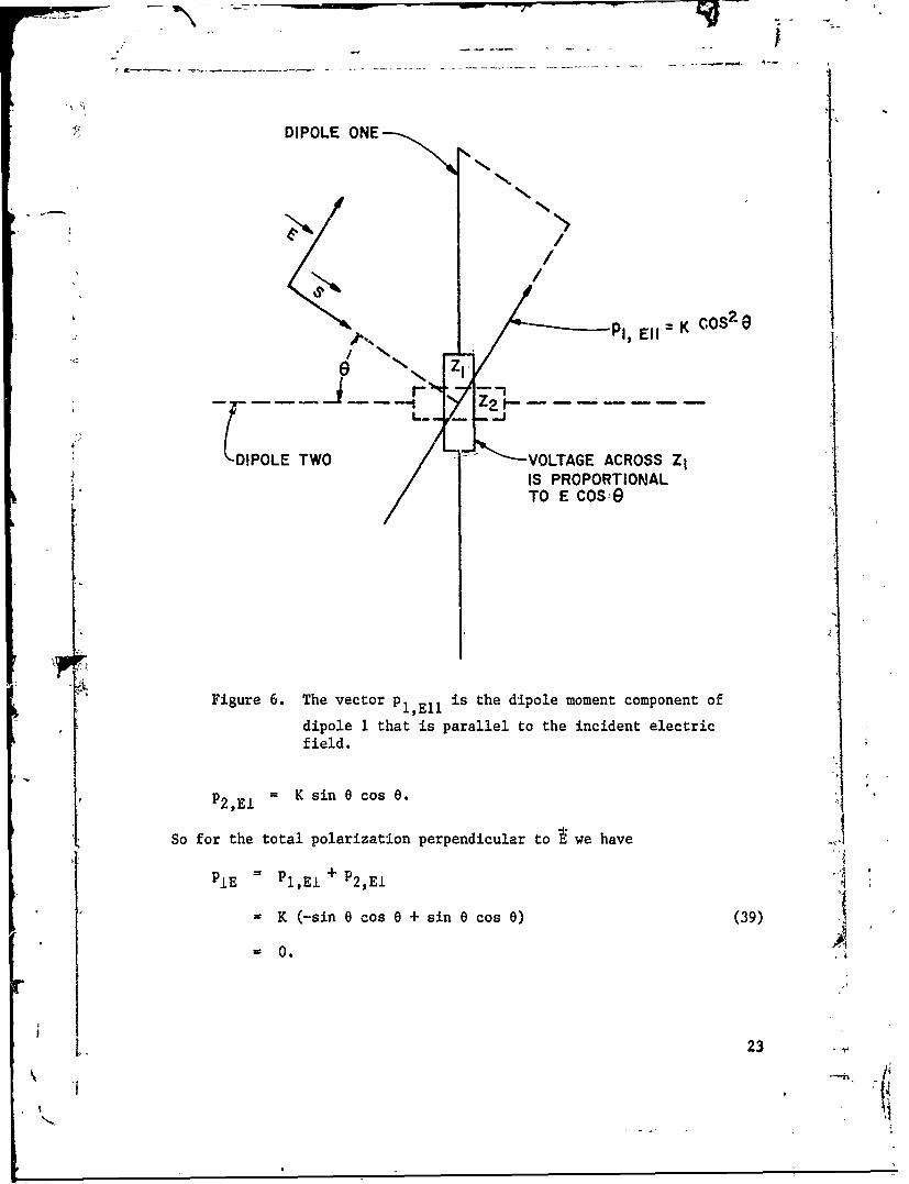
6. The vector P1,E11 is the dipole moment component ofdipole 1 that is parallel to the incident electric field ... 23

7. The dipole moment of dipole 2 can be resolved intocomponent,8 parallel and perpendicular to the incident

8. The vector p1,EL is the dipole moment component of4dipole 1 that is perpendicular to the incident field ....... 25

9. Spherical cavity in dielectric ........................... 26

7Preceding page blank

N6

FIGURES

10. Three-dimensional array of inductively-loaded dipolesenclosed in styrofoamspheres ............................... 29

11. Values of relative permittivity calculated with,equations (36)i and (42) for a number of different'inductive loads. The other parameters are discussedin the text ....... . .................... 35

12a. The real component of relative permittivity cilculated,with equations (69) and (42). The value used for Lis .4 PH and the value used for R is 00. The otherparameters are the same as those employed to obtainfigure 11 ........... 0....................................... 36

12b. The real component of relative permittivity calculateswith equations (69) ,and (42). The value used for Lis .4 PH and the value used for R is 500. The otherparameters are the -same as those employed to obtainfigure 11 ............... ........, .............. . 37

12c. The,,'eal component b .r:..ative permittivity calculatedwith oquations (69), and (42). The value used for Lis .4 jAH and the value used foi, R is 1000. The otherparameters are the same as those employed to obtainfigure 11.............................................. 38

12d. The real component of relative permittivity calculatedwith equations (69) and (42). The value used for Lis .4 PH and 'the value used for R is 200R. The other

parameters are the same as those employed to obtainfigure 11............. 38

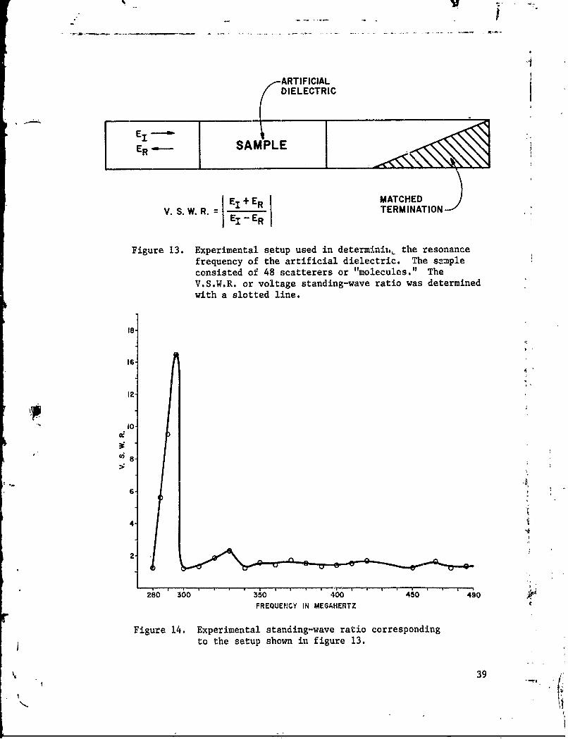
13. Experimental setup used in determining the resonancefrequency of the artificial dielectric. The sampleconsisted of 48 scatterers or "molecules." TheV .S.W.R. or voltage standing-wave ratio was determinedwith a slotted line .... ..................... ...... . . 39

14. Experimental standing-wave ratio corresponding tothe setup shown in figure 13 ... ....... ...... ..o............ 39

15. The accuracy of the experimental points is limitedby the granularity of the sample and the correspondingindefiniteness of the sample edges.......................... 41

8

1. INTRODUCTION

The complete simulation of the electromagnetic pulse, EMP, associatedwith a nuclear burst involves a number of interrelated parameters. Themost obvious parameters are the waveform and the magnitude of the EMP.However, if the system being subjected to the nuclear EMP is in a pre-ionized region such as the ionosphere, we would also have to simulatethe ionozation or dielectric constant of the medium surrounding the sys-tem such as a missile or satellite. In this work we investigate thefeasibility of using an artificial dielectric consisting of a randomdistribution of inductively loaded short dipoles to simulate the macro-scopic electromagnetic properties of a simple Lorentz plasma.1,2

During the past twenty-five years a number of so-called artificialdielectrics consisting of regularly spaced rods, parallel plates, metalspheres, etc. have been devised to reproduce the essential macroscopicproperties of a dielectric. The ordinary artificial dielectric consistsof discrete metallic or dielectric particles or lattices of macroscopicsize.3-7 These artificial dielectrics were first actually conceived aslarge-scale macroscopic models of microscopic crystal lattices. Thepractical motivation for the development of the first artificial die-lectrics was the desire to obtain relatively inexpensive lightweightmaterials that could be used for microwave and radar lenses. Several ofthe artificial dielectrics proposed for microwave lenses have the macro-scopic electromagnetic properties of a plasma.

2'4 ,8'9 ,i0

A review of the literature reveals a number of papers on the plasmasimulation properties of artificial dielectrics consisting of a rigidcubic lattice of three-dimensional grids. 2 ,4 ,8 Experimental work, re-ported in the literature has been done only on two-dimensional grid.lattice structures.2 ,8 ,16 That a periodic grid structure would produceband structure resonances analogous to Bragg scattering has been dis-cussed from a theoretical viewpoint, but has not been experimentallyinvestigated.

11 ,12 ,13,14

The rigid cubic grid lattice structure has the disadvantage ofbeing somewhat unwieldy and difficult to support and fit around an ob-ject with curved surfaces. In general, the cubic lattice grid structurelends itself conveniently to simulation of flat, slab-like plasmasheaths.

In this paper we describe another approach to the simulation of aLorentzian plasma. We propose a granular pellet-like artificial die-lectric consisting of a random distribution of styrofoam spheres con-tainng inductively loaded dipoles which can yield macroscopic electro-magnetic constitutive relationships similar to those of a plasma.

A Lorentz plasma can be represent-d from the viewpoint of macro-scopic electromagnetic theory, as a lossy dielectric with a cnmplexdielectric constant given by

9

ep= Co i-W 2/(v 2 + W2) + jwZ(v/W)/(v2 + W2)J(1p p

where co is the dielectric constant of free space, w is the frequency ofthe electromagnetic field, Wp is the plasma frequency, and v is the

collision frequency between electrons and the gas molecules. We propose

to simulate this macroscopic dielectric constant with an artificial

dielectric consisting of a random distribution of inductively loaded

dipoles encased in styrofoam pellets. A schematic drawing of such a

dipole is shown in figure 1. The quantities 2k, L, and R are the length,

inductance, and resistance of the loaded dipole respectively. As we

will show, using simple quasi-static arguments, if the effective in-

ductance wL is much greater than the effective capacitance of the dipole,

the permittivity of a random distribution of inductively loaded dipoles

is

42 2 N 42 2 N R 13 co L 3 co L L w

Cp = eo + j " (2)

( R2 R2 2+ 2 (-) + W2

where N is the number density of the dipole pellets. One can see by

comparing equation (1) with equation (2), that we can simulate a plasma

with plasma frequency w p and collision frequency v by setting

4 22 (3)3 cL p

S and

R = V. (4)L

R RL2

Figure 1. Inductively loaded dipole.

10

2. THEORETICAL DISCUSSION

2.1 Quasi-Static Approach

We will first approach the problem of our proposed artificial die-lectric from a quasi-static viewpoint assuiing that the inductive loadof the dipole is much larger than the driving point capacitive impedanceof a short dipole. In a subsequent section we will explicitly considerthe dipole capacitance. First, we discuss the simulation of a tenuousplasma in which the collision frequency between free electrons and mole-cules, v, is negligible.

We want to construct an artificial dielectric from a pellet-likemedium that has an index of refraction given by

2

n = (1 - W2/w2) 1/2 (5)p

and an intrinsic impedance given by

1/2

(6)

where ep has a frequency dependence of the form1 ,2

ep = o (1 - u2/w2) (7)

and where wp is the plasma frequency.

In general the index of refraction of an artificial dielectric maybe calculated in a manner analogous to that employed in calculating theindex of refraction of a molecular medium. Assuming that the randomobstacles are not too closely packed so that we do not have to resort tothe Clausius-Mossotti relation, the index of refraction is given by

5

n [ (1 + NXe/O) '1 (1 + NXm/pO)] 1/2 (8)

where

N = Number of scattering obstacles per unit volume,

Xe = Electric polarizability of a scattering obstacle,

Xm = Magnetic polarizability of a scattering obstacle,

el = I (for styrofoam),

= I (for styrofoam),

11

N -

co = permittivity of free soade,

v0 = permeability of free space.

From equations (5) and (8) we see that in order to achieve our goalwe need an artificial dielectric constructed from obstacles that have anegative electric polarizability, Xe. If the artificial dielectric is tosimulate a plasma over a spectrum of frequencies, the value of Xe mustalso be inversely proportional to the frequency squared. We would alsolike the vaJae of the magnetic polarizability of -the embedded obstacles,Xm, to be all or, 'if possible, zero.

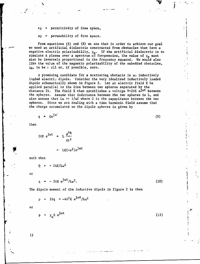
A promising candidate f6r a scattering obstacle is at inductivelyloaded electriz dipole. Consider the very idealized inductively loadeddipole schematically shown in figure 2. Let an electric field E beapplied parallel to the line between two spheres separated by the-distance 2k. The field E then establishes a voltcge V=2.E eJit betweenthe spheres. Assume that inductance between the two spheres is L, andalso assume that Lw >> I/wC where C is the capacitance between the two

*spheres. Since we are dealing with a time harmonic field assume that-the charge accumulated on the dipole spheres is given by

q = Qej " (9)

then

2E ejWt = L d 2 q

dt2

LQ(-w2)ejWt

such that

Q - 2£E/Lw2

or

q - 2UE ejWt/hW2. (10)

The dipole moment of the inductive dipole in figure 2 is then

p = 2kq = -4Z2E eJWt/Lw2

or

p = XeE ei~t (11)

12

/ STYROFOAM/ PELLET

!

L21-

Y1I

Figure 2. Lossless inductively loaded Aipole.

The lossless dipole corresponds to a collisionless plasma.

where

Xe = - 4Z2/Lw2. '12)I

If we have a random distribution of dipoles, we must, naturally, con-sider the various orientations that the dipoles can assume. As shownin figure 3 let the E field be in the Z direction. For every randomdipole direction e, we have an equally probable direction -0 We cantherefore pair all the dipoles-dbriented in the +0 direction with dipolesoriented in the -0 direction, The resultant effective dipole moment fora dipole is

p(O) -2 cos e (k 2k cos 0) E ei t/Lw2.

The average value for a random distribution of directions, Pay, is then

7r/2 7r/2pay - 4 cos-tj~xE eJ w~'/L92) sin dew2 2i sinsi d

Pav f /2 f1 27 sin 00

o

= 3P = - 4k2E eiwt/3LW2.

Therefore, we have

Xeav = - 4 2/3Lw2. (13)

13

'Ia

Xr

Ey

Figure 3. Two dipoles oriented in the 0 and -0 directions.

The y components of the two dipoles cancel.

Now assuming that Xmav = 0, the index of refraction of the artlficlal

dielectric would be

n = ([I (- 4NZ2/30LU)2)1 ] 1/2t

and the intrinsic impedance would be

N A-

n = [vO/coCZ - 4N£t2/3c0Lw2)]1 /2t

In the case of tenuous plasma (ionized hlgh-altitude air) we have anindex of refraction given by

n = (1 - Ne2/ComW2) I/2 = (1 - 3.18.109N/w2)I-/2 (14)

' where N is the electron density in CM- 3, m is the electron mass, and e

is the electron charge. Therefore, if we want to simulate a tenuousplasma corresponding to electron density N, we can determine the length2Z and the inductance L of our inductively loaded dipoles with therelation

NZ2 2

2.39109N sec

hL 4 com

14

=4 j' c" -42I~ow)'

- *

or

N-2 2.11.10 2N sec- 2 F/m (15)

L

where N is the density of artificial dielectric dipoles in meter-3 , Y isin meters, and L is in henrys.

Next, we note that by introducing a resistance into our dipole wecan simulate the imaginary part of the index of refraction that arisesbecause of the collisions, v, per second between the pl'sma electronsana the atmospheric molecules. Figure 1 shows that the voltage betweenthe dipole spheres is

U 2 eEedt = L R&dt2 dt

where as before we assume Lw >> l/Cw. Again, we can assume that the-charge on the capacitance between the two spheres varies as

j wtq = Q e

Then

2kE ejwt = LQ(-w2)ejwt + Ijw ejbt

and

Q = -2LE/(Lw 2 - jRw)

or

q = -2ZEeJt/(Lw2 - jRw).

The dipole moment along the axis of the inductive dipole in figure 1 isthen '.

p = 2q = - 4 2E eJwt/(Lw2 - jRw).

We see by analogy with the purely inductive dipole

ay p = - 4 2E eJwt/3(LW2 - jRw).

15

K1

Therefore, we have

Xeav = - 4Z2/3(LW2 - jRa) (16) 1and

£p eO 1 - 4Z2N/3coLW2(1- jR/wL) (17)

3 £oL 3 eoL 'L= (o J42- - + J .. .j (18)

R2+ W2 R(2 + W2/

Finally, we note that if equations (3) and .4) are satisfied, we have a

one to one correspondence between equations (1) and (,').

2.2 Explicit Consideration of Dipole Capacitance

Up to this point we have assumed that the inductance used to load theshort dipole dominated the behavior of the dipole. We will now examinethis assumption in more detail. The arguments presented here are basicallydue to-Harrington.1 5 Consider two short dipole antennas as shown infigure 4. Antenna 1 is excited by a current source II; antenna 2 is loadedat its center with an impedance ZL. The ciirrents and voltages of the twodipoles can be related by the standard impedances of a two-port network:

V1 = Z11 Ii - Z12 12(

(19)V2 = Z21 Il - Z22 12.

The voltage V can be expressed in terms of ZL and 12: V2 = ZL 12. Thenwe can express the current passing through the load ZL in terms of thecurrent source driving antenna 1; the transfer impedance Z2 1; the drivingpoint impedance of antenna Z, Z2 2; and the load impedance, ZL:

12 =~Z21 Ii(20)(ZL + Z22

We next make use of the reaction concept, first introduced byRumsey.1 6917 Rumsey d~fined reaction of field a on the source b, {a,b},with the following integral:

16

ZL j12

ANTENNA I ANTENNA 2

V1 Zi I I -Z12 12

V2 Z2 1 I - Z2 2 12

Figure 4. Two short d',t'pole antennas.

{ajb} JR ~J - .Mb) dv

where jb is the electric current dens-ity of source .b and Mb is the mag-netic current density of source b. In this notation the reciprocity-theorem is:

{a,b) = {b,a}.

For a current source 1b, we can obt~in

{a,b) fEaI b d2. = I bJfEa. -d VaIb. (21)

T1he transfer impedance in equation (19) is defined byI

z V /I

ii iji

where Vij is the voltage at terminal i produced by the current source atterminal j. In equation (21) we indicate that

{j,il -V IV

a 17

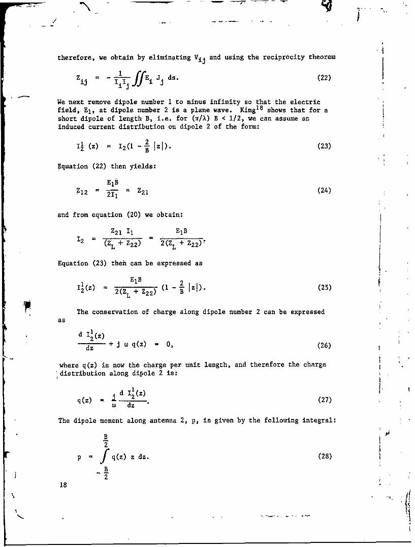
therefore, we obtain by eliminating Vij and using the reciprocity theorem

i ff JI ds. (22)

We next remove dipole number 1 to minus infinity so that the electricfield,- El, at dipole number 2 is a plane wave. King18 shows that for ashort dipole of length-B, i.e. for (IT/A) B < 1/2, we can assume aninduced current distribution on dipole 2 of the form:

i2 (z) = 12(1 -g IzI). (23)

Equation (22) then yields:

E1B1 21 Z 2 1 (24)

and from equation (20) we obtain:

Z2 1 Ii EIB12 (ZL + Z2 2)

2 (ZL + Z22)'

Equation-(23) theh can be expressed as

EIB 2

I2(z) = 2(ZL + Z2 2 ) (1 - B IzI). (25)

The conservation of charge along dipole number 2 can be expressedas

d I2(z)

dz + j w q(z) = 0, (26)

where q(z) is now the charge per unit length, and therefore the charge'distribution along dipole 2 is:

q(z) = 2 d_____) (27)W dz

The dipole moment along antenna 2, ?, is given by the following integral:

B2

p fq(z) z dz. (28)

B2

18

7'-

Expressions (25), (26), and (28) then yield:

-j El B2

p = 4w(j wL + Z2 2) (29)

If we allow X to be the polarizability of the dipole we have: (

p =EX (30)

or

_j B2 (31)

4w (jwL + Z22)*

Equation (31) is essentially the same as the result we obtained-with thesimple quasi-static model, except for the presence of the driving pointimpedance Z2 2 in the denominator. (The factor 4 in the denominator occursbecause we have not capacitively end-loaded the dipole as in figure 1.)

King1 9 ,20 derives a value for the impedance Z2 2 of a short dipole:[ () B2 41n ( B 6.78].(2Z2 2 = - 12 ( b (32)

Here n is the impedance of free space, 120 wQ, B is the length of thedipole, and A is the dipole radius.

Up to this point we have considered the incident electric field E,to be parallel to the short inductively-loaded dipole. Of course, thecurrent and charge distribution along the dipole is a function of theorientation of the receiving antenna with respect to the surface ofconstant phase of the incident electric field. King19 indicates thatfor a short receiving antenna (with a triangular current distribution)the projection of the electric field onto the antenna, multiplied bythe actual half length of the antenna. gives the emf of the equivalentcircuit. That is equation (24) is modified to

EIB

Z12 = Z21 = 12 cos 0 (33)

where 0 is the angle between the incident electric field vector andthe antenna. For example, 0 = 0' when the antenna lies in the sur-face of constant phase. We can now use the same orientation argu-ments that we used in the development of our quasi-static model which

19

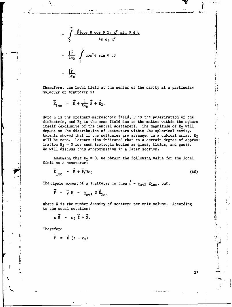
ignored the self impedance Z22. If we wish to calculate the polarizationin the direction of the incident electric field when the E1 vector is notparallel to the dipole, we must introduce another cos e and integrateover all directions. Therefore, as before

1rav =

and

PaV = avE

or

j B2

Xav 12w(jwL + Z22)" (34)

If we set Z22 = 0, B = 2k, and end-load the dipole so that the currentdistribution is uniform and not triangular, we obtain the same resultas given by equation (13).18

The appearance of Z22 in the denominator of expression (34) is in-consistent with our desire to model a simple Lorentzian plasma. Spe-cifically, when the frequency is such that

L= -f1%(35)

the artificial dielectric will pass through a resonance. We can onlyuse the inductively-loaded dipoles to simulate a plasma if wL " Z2 2.We will discuss the effect of Z22 in a subsequent section. An insightinto the limitations imposed by the dipole self-impedance can be ob-tained by calculating Xav for some realistic frequencies and dipoleparameters.

2.3 Mutually Perpendicular Dipole Scatterers

Our arguments presented so far assumed that the distance btweenthe inductively-loaded dipoles is great enough so that their interactioncan be neglected. The use of equation (8) is based on the assumptionof negligible interaction between scattering objects. A way of in-creasing the value of N in (8) by a factor of 3 and still not violatethe assumption of negligible interaction of neighboring scatterers isto construct each scatterer out of three mutually-perpendicularinductively-loaded dipoles. By using essentially quasi-static argu-ments it is easy to see that three mutually-perpendicular dipoles witha common center point do not interact.

20

Consider just two perpendicular dipoles as shown in figure 5. By Nsymmetry the current distribution along the two arms of dipole 1 issymmetrical and equal in magnitude. Therefore, the charge distributionalong the opposite arms is equal in magnitude but of opposite sign.Using a static argument the electric field produced by the charge distri-bution along dipole 1 is seen to be perpendicular to the direction ofdipole 2. The dipoles therefore do not interact. Similar reasoningapplies to a dipole that is mutually perpendicular to dipoles 1 and 2and centered at the intersection of dipoles 1 and 2. These quasi-staticarguments are donsistent with the more rigorous arguments presented forskew-angled dipoles by Richmond.21 If we substitute three mutually-perpendicular dipoles for the single randomly-distributed dipoles wesimply multiply the average value of the polarizability given in equation(34) by 3 and obtain

- j B2

Xav3 = 4w(jwL + Z22)" (36)

By constructing our scatterers out of three mutually-perpendicularinductively-loaded dipoles we accomplish more than simply inc:reasing thenumber of scatterers by three: the polarizability of the scatteringcenters is made to be independent of scatterer orientation. To bespecific, the scatterer, consisting of three identical, short, mutually-perpendicular dipoles centered at the origin with a dipole along eachaxis, can be described with the following simple dyadic:

X = X (ii+ j j + k k) = X I.

The dipole moment induced by an arbitrary field E is then

p 1 X'E

X E (i sin 6 cos 4 + j sin e sin4 + k cos e) (37)

= XE (f sin e cos 4) + j sin 6 sin (P + k cos 0)

but (sin e cos )2 + (sin 6 sin 4)2 + cos20 = 1. Therefore, the magnitudeof the dipole moment is c E and its direction is in the direction of theelectric field regardless of the orientation of the scatterer.

In order to gain insight into the foregoing result we can considera relatively simple situation in more detail. Figure 6 illustrates twoperpendicular inductively-loaded dipoles in the plane of the page. Letthe E vector of the incident plane wave also be in the plane of the page.The third dipole is perpendicular to the plane of the page, and thereforeis perpendicular to the E vector and does no interact with the E field.As shown in the figure, the Poynting vector S of the incident plane waveis also in the plane of the page. The voltage developed across the loadof dipole number I is then proportional to E ccs e and the separation of

21

P

,,--DIPOLE ONE

DIPOLE TWO

Figure 5. Two perpendicular inductively-loaded dipolesdo not inte'ract.

charge on dipole number I in the direction of the incident E vector isPOP- proportional to cos 26, that is Pl,Ell w K cos 28. A corresponding argu-

I ment (see fig. 7) leads to the conclusion that the dipole moment ofdipole number 2 in the direction of the incident field E is given byP2 El K sin2e. The total dipole moment in the direction of the vectorE of ipoles I and 2 is, therefore, given by

PEI P1, + p2,Ej = K cos 2e + K sin2e

= K =

4w(JwL + Z22)"

Let us now consider the polarization perpendicular to the Evector. Asshown in figure 8 the voltage developed across the load on dipole 1 isproportional to E cos 8 and the dipole moment perpendicular to the Efield or parallel to the S vector is Pl El = - K cos 0 sin e. As shownin figure 7, since the voltage across te load on dipole 2 is proportionalto E sin 0, the dipole moment component of dipole two perpendicular tothe incident field is

22

_

K 1'I

DIPOLE ONE

KNOS2PI l

ZI N

_r01OLETWO _Vr VOLAGEACROS Z

f edP2,EJ 2"K in6 os6

So ~ ~ ~ ~ ~ .fo th oa oaizto epniclrt1ehv

IE=POlEI 2E

TW VOTG ACROSS Z1o sn6cs )(9

I= PRPRTOA

TO E C23

k- DIPOLE ONE

I I

DIPOL TWO L JVOLTAGE ACROSS Z2DIPOLE TWO T IS PROPORTIONALTO E SIN e

P2, Ell KSIN -P 2 , El K COS eSINe

Figure 7. The dipole moment of dipole 2 can be resolved intocomponents parallel and perpendicular to the incidentelectric field.

In summary, we see that the rather tedious arguments leading to equations(38) and (39) are consistent with the result of equation (37). Of course,as the length of the dipoles is increased, the simple trigonometric de--pendence for the current or charge distribution does not hold, and thepolarization is not independent of the direction of the incident electricfield.

2.4 Coupling of Scatterers

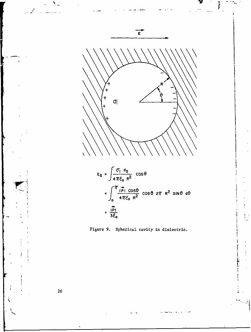
The dipole interaction of the scattering objects, each consisting ofthree mutually-perpendicular and centered, inductively-loaded dipoles,will be considered next. The starting point for the discussion of thecoupling of scattering objects in both real and artificial dielectricsis the formula of Lorentz for the field within a hollow spherical cavity(centered at a particular molecule or scatterer) cut out of the dielectric

24

.C

- DIPOLE ONE

; VOLTAG ACROSS ZI "

IS PROPORTIONALN TO E COS9

/,...

."Is"

IPOLE'TWO

P1, El=-K COSe SIe

Figure 8. The vector P1,E1 is the dipole moment component of o

dipole 1 that is perpendicular to the incident field.

(fig. 9). The displacement vector D normal to the dielectric surfacebetween the sphere and the cavity must be continuous; therefore, themagnitude of P normal to the cavity surface equals the negative of thei-*-

induced surface charge density oi. We may write aj = - 1Pj cos 0.The field inside the cavity due to ai can be calculated at the centerof the cavity with Coulomb's law:

= f ids cos 0E i oEs f 4v c o R2

S

525

E

J+re R

-G T

262

PII

ft-

cos 0 cos 0 2 R2 sin d

0 4n c0 R2

--

f cos26 sin 0 dO23o

Therefore, the local field at the center of the cavity at a particularmolecule or scatterer is

1'E E E+-P +E 2 -Eloc C0

Here E is the ordinary-macroscopic field, P is the polarization of thedielectric, and E2 is the mean field due to the matter within the sphereitself (exclusive of the central scatterer). The magnitude of E2 willdepend on the distribution of scatterers within the spherical cavity.Lorentz showed that if the molecules are arranged in a cubical array, E2will be zero. Lorentz also indicated that to a certain degree of approx-imation E2 = 0 for such isotropic bodies as-glass, fluids, and gases.We will discuss this approximation in a later section.

Assuming that E2 = 0, we obtain the following value for the localfield at a scatterer:

Eloc E + P/3 0 (40)[

The dipole moment of a scatterer is then p = Xav3 Eloc, but,

i P =pN = Xav N o

where N is the number density of scatters per unit volume. Accordingto the usual notation:

C E = e0 E+P.

Therefore

* + 4+P E e o

27

/i

and

P = Xav3 N Eloc = Xav3 N (E + P/3e0)

E E(41). .--- E(CI-C0)

= Xa N (E + )av3 c

This is the Clausius-Mossotti relation. Equation (41) can be manipulatedto yield:

1 + 2 N Xav3/3(0C = Co 1- NXv (42)

o I N Xav3 /e

he above expression is only valid when the local electric field Eloc at ascattering obstacle can be expressed as

+ + +

E = E + P/(3c0 ) (43)loc

where E is the space average field inside the artificial dielectric.

The local fields for simple tetragonal and hexagonal lattices havealso been calculated by a number of workers. CollinT,22 considers athree-dimensional array of y-directed unit dipoles at x = na, y =mb,and z = sc. He excludes the dipole at x = y = z = 0 and calculates thelocal field at x = y = z = 0. The potential due to a unit dipole atx0, Y0 , z0 is

Jr (44)

-4v co r3

* where r : [(x - xo) 2 + (y -yo) 2 + (Z - Zo)2]1/2. Fot the array of

y-directed dipoles we then have (fig. 10)

S Z E y-mb (45)n=-c s=- m-co I(x-na)2+(y-mb)2+(Z-sc)213/2

where the prime indicates the omission of the n = m - s = 0 term. The

effective polarizing field at x = 0, y = 0, z = 0 will then be E + Eu,where E is the external applied field and where

, 3~~=

i B

28

I-K

I II f ,

I0,'

~CUBIC LATTICE o~b~c

• TETRAGONAL LATTICE a c b

, . HEXAGONAL LATTICE oa b~c

SFigure 10. Three-dimensional array of ind- tively-loaded V"

' dipoles enclosed in styrofoam spheres.

!.00

S29 I.0L

xA

ba

• z -•

11 2 (mb) 2-(na) 2-(SC) 2

ffi -- 0 E Z (46)mff-O* n=- M s = - 0 [b)2+(na)2+(sc ) 2 -9/2"

Note that the above expression is not only evaluated inside the Clausius-

Mossottl sphere, but over all space. We therefore do not have to considera contribution from the inside surface of the sphere.

Collin evaluates expression (46) and obtains

E 1.201 _87r[ 27rc + 27a] ()i £0 7 0 b b

where K0 is the so-called modified Bessel function of order zero. Equa-tion (47) is for unit dipoles. In our case of inductively-loaded dipoleswe would have

i 10 ir 3 b 1.201 _8w K 27rc + 27ra)]1(8E -i Ko +' K0 Xa (48)SCu ir b 3 b3 b 3v

or

o1 1.201 8w K 2(rc£0 ( E b 3 b3 K

\ (49)

+K0 27ra B2..+4w( wL+Z 2) /'

The above equation corresponds to a cubic lattice if a = b = c, a tetra-fl gonal lattice if only two of the quantities are equal, and a hexagonallattice if none of the quantities, a, b, or c are equal. In the case ofthe cubic lattice we find that

1.06 NEloc E+ Xav3 (50)

0

and, therefore

2.08 N1 + X E0 av3 (51)

0 1.06 N01 i Xav3

' which is to be compared with equation (42).

30

2.5 Deviations from the Clausius-Mossotti Equation Due to Randomnessof Scatterers

J.K. Kirkwood2 3'2 4 has calculated the deviations that one might expectfrom equation (40) in the case of a random distribution of molecules con-sisting of hard spheres. Specifically, Kirkwood considered a molecularinteraction potential of the form

(r) 0 < r < a(52)

- 0 r>a

where a is the diameter of a molecule.

Kirkwood's model is not wholly applicable to an artificial dielectricformed by dumping spherical scatterers into a container because thescatterers do not necessarily assume a completely random distribution.For example, depending, among other factors, on how smooth they are, thespheres can arrange themselves into various specific lattices or combina-tions of lattices. The different lattices can even correspond to dif-ferent dipole number densities.

It is interesting to note that statistical mechavical averagingbased on the molecular interaction equation (52) yield: a value of thepermittivity that is not a function of the thermodynamic temperature T.This follows because the value of the exponential term exp[-W(r)/kT] iseither 0 or 1. In a gas or fluid the averaging can be over time; in ourstatic collection of scattering dipoles the averaging would have to be

over an ensemble of different containers each filled with a aggregationof spherical dipole scatterers. Kirkwood's approach can be summarizedas follows: As in the lattice case, the local field is obtained by

for, summing over the potentials due to individual dipoles. We can say thatthe effective polarizing field Eloci at scatterer i will be given by E + Ei,where E is the external applied field and Ei is given by the sum over Nindividual dipoles:

N

k=1 ~~

where the dipole-interaction dyadic is given by

4.+T 1 1 1-3 rik r i k (54-ik =4r 0

2 0 r 3ikik

ik

31

The polarization of an individual scatterer is given by

.+

C:OaE - co E ik' k

We therefore have N simultaneous equations

p+ ac Ei' T ac0E i. = I..

that would have to be solved in order to obtain Eloci for each of theindividual scatterers in the distribution of N scatterers in volume V.We can average the N equations and obtain

4. acot~p (56)

Kirkwood23 $24 incrc,/',cd the following fluctuation term

N -

n E (T - Ti~ (57)i=1 U k =kP

i~k

and obtained

aeot (58)p +aeo E Tik.P + nco=

If we can assume that

.112P1 = 112*Pl (59)

the fluctuation n is equal to zero and

ik + aeoPc 0T (60)

Convierting to the equivalent scalar equation we obtain:

ae0E_ (61)

1 + aCO(E Tik)

32

and

D =cE eE + P (62)

N-S 0E + - pV

N0 aE

S 0E + • (63)1 + a0 (Z Tik)

The dipole interaction term can be averaged over the volume v to yield:

-- T (64)£Tik - 3v (

also

Xav3a= -- (65)£0

and therefore

e =co + (66)1 - 1/3 NV a. v

or

1 + Xav33 v £0

C Co . (67)1 i N Xav3

3 v £o

Equation (67) is to be compared with equations (51) and (42). Afterconsiderable mathematical manipulation and a number of approximations,Kirkwood managed to evaluate equation (57) for a substance consistingof a random distribution of hard noninteracting spheres of diameter a:

1 5 N 2a2D (68)n (-b -2T-) (68)A9- 48 v v

33 >

x t

where

2rNa3 a3

b 4 N &g )

-4 (volume of spherical scatterers).

To obtain a rough estimate of the validity of using the Clausius-Mossottiequation for a random distribution of styrofoam ball dipole scateerers,we can compare the value of n given by equation (68) with the value of 23

l va

For the experimental situation discussed in Section 2:

n = .221 - a Z Tik

and we might expect the Clausius-Mossotti equation to be a reasonablefirst approximation. Actually, as we have pointed out, Kirkwood'sstatistical model is not necessarily applicable to our aggregation ofdipole scatterers because the dipole scatterers in the artificial die--lectric do not necessarily assume a random distribution. The validityof the Clausius-Mossotti equation as applied to our artificial dielectricshould really be tested empirically.

3. COMPARISON OF EXPERIMENT WITH THEORY

In order to orient ourselves in regard to the parameters such as thedipole load impedance and Z22 we will use equations (36) and (42) todesign an artificial dielectric with some actual experiments in mind.The frequency range considered will be dictated by the band pass char-acteristics of the type 2300 waveguide. The type 2300 waveguide, thelargest standard waveguide, has internal dimensions of 23.0 x 11.5 in.,a lower cutoff frequency of 2.56 x 108 H, and a recommended upper fre-quency limit of 4.9 x 108 H. The frequencies in this range are muchhigher than the values usually quoted for nuclear EKP pulses, but we willconsider designing an artificial dielectric to operate at these high fre-quencies because of the convenience of using waveguide techniques inmeasuring the properties of an artificial dielectric.

Let us consider the following series of parameters as an orientationexercise. We begin with an artificial dielectric constructed out of $A

scatterers consisting of three mutually-perpendicular inductively-loaded7-in. long dipoles loaded with a number of different values of inductance.Let the dipole stems have a radius of 0.1 cm. We choose the density of

34

scatterers to be 264 per cubic meter. This density corresponds to anaggregation of 48 scatterers distributed throughout a rectangular con-tainer with dimensions 23 x 11.5 x 41.5 in. Equations (36) and (42)can be employed to calculate the dielectric constant of the artificialdielectric as a function of frequency in the band-pass region of thetype 2300 waveguide. Figure 11 shows values of the real part of thepermittivity calculated with equations (36) and (42) for a frequencyrange between 300 and 500 MH. The four curves correspond to dipoleload inductances of 0.4, 0.6, 0.9, and 1.4 iH. The magnitude of theradiation resistance of the dipoles is very small compared to the valuesof the magnitude of the inductive loads; therefore, the imaginary com-ponents of the permittivity are very small.

L. =. u

.8"

.7-

A.6-

.8-

W .5-

.2

.4-

0-300 320 340 360 380 400 420 440 460 480 500

FREQUENCY IN MHz

Figure 11. Values of relative permittivity calculated withequations (36) and (42) for a number of differentinductive loads. The other parameters are dis-cussed in the text.

35

!-i

2V

If we want to model a Lorentz plasma in which the electrons have acollision frequency v # 0, the load impedance of our dipoles must have aresistive component. Equation (36) then becomes:

- j B2

Xav3 4w(JwL + R + Z22)

where R is the value of the resistance. In figures 12a to 12d we presentvalues of the real part of the permittivity calculated with equations (69)and (42) with L = G.4 VH. The series of four figures shows the effect ofdifferent values of the resistive component R on the magnitude of theresonance occurring when JwL = Z22. Figure 12a, corresponding to a purelyinductive load, emphasizes the resonance behavior of the artificial die-lectric produced when the load inductance L is in resonance with thecapacitive impedance of the dipole. As can be expected the Q of theresonance is reduced by including a resistance in the dipole load im-pedance.

8

6> L =.4,uH-

61> R Oil

E 10w

0

w

W 2.~ 2.4 2.6 2.8 30 3.2 3.4 3.6 3.8 4.0 4.2 4.4 4.6 4.8 5.0

00 - Hz x 108

0 THE Q OF THE RESONANCE

0 -4- WHEN R=O IS DETERMINEDU BY THE RADIATION RESIS-J< TANCE OF THE DIPOLE.w

S-6.

Figure 12a. The real component of relative permittivity calculated

with equations (69) and (42). The value used for L is.4 pH and the value used for R is 02. The otherparameters are the same as those employed to obtainfigure 11.

36

2.5 1L =.4.uH

- R 50,'>2.0.

1.5-

>

lit-

1.0 ---,- - - -- - - -- -,

0 *

zWZ .500

< 2.4 2.6 2.8 3.2 3.4 3.6 3.8 4.0 4.2 4.4 4.6 4.8 5.0

Hz x 108

Figure 12b. The real component of relative permittivity calculateswith equations (69) and (42). The value used for L is.4 VH and the value used for R is 50. The otherparameters are the same as those employed to obtainfigure 11.

I- L = .4pHR =10 (1.5

W

..

W

00

o I r rII. I I ! I i ' I I II * -i r- -. 2.4 2.6 2.8 3.0 3.2 3.4 3.6 3.8 4.0 4.2 4.4 4.6 4.8 5.0

W Hz x 108

Figure 12c. The real component of relative permittivity calculatedwith equations (69) and (42). The value used for L is.4 VH and the value used for R is 100. The otherparameters are the same as those employed to obtainfigure 11.

37

L =.4pH

R = 20011

2 1.5

i- 1.0 ---'

U.

0 .5"

zz0

.0

o 2.4 ' 2.6 2.8 30 32 34 3.6 3.8 40 4.2 4. ..4 4.6 4.8 5.0

C,

-t

* Hz x 108

Figure 12d. The real component of relative permittivity calculatedwith equations (69) and (42), The value used for L is.4 pH and the value used for R is 200Q. The otherparameters are the same as those employed to obtainfigure 11.

In our first experiment we searched for the resonance predicted byequation (36) and shown in figure 12a. The 'cperimental technique2 5

was straightforward and is depicted in figure 13. The ratio of theincident electric field E, to the reflected electric field ER was ob-tained by measuring the standing wave ratio with a slotted line. Theartificial dielectric sample shown in figure 13 consists of an aggrega-

tion of 48 of our 7 in. styrofoam balls each containing 3 mutually-perpendicular dipoles. The balls were enclosed in a rectangular boxmeasuring 23 x 11.5 x 41.5 in. The results of the experiment are shownin figure 14. It is comforting to note that there is a large reflectionat approximately the frequency of the resonance shown in figure 12a.

In a second series of experiments we measured the permittivity ofour artificial dielectric utilizing the well-known shorted waveguidetechnique described in great detail by von Hippe126 . Very bripily, thetechnique consists of measuring the null point of a standing wave in ashorted waveguide. A sample of length 2 is then inserted into theshorted waveguide and the shift in the standing wave null is noted. Theindex of refraction of the dielectric sample of length k cML, then becalculated in terms of 2 and the shift in the standing wave null point.

38

ARTIFICIALDIELECTRIC

ER ER 6---SAMPLE

I MATCHEDV. S. W. R. =E+ERITERMINATION)

Figure 13. Experimental setup used in determini,, the resonancefrequency of the artificial dielectric. The sampleconsisted of 48 scatterers or "molecules." TheV.S.W.R. or voltage standing-wave ratio was determined

with a slotted line.

18

"I

16

6-

12

4-'

280 0 350 400 450 490

FREQUENCY IN MEGAHERTZ

Figure 14. Experimental standing-wave ratio correspondingto the setup shown in figure 13.

,I 39

Our experimental values of the index of refraction and some calculated

values are shown in figure 15. The measurements were of two differentartificial dielectric sample sizes; one sample consisted of an aggrega- Ition of 24 scatterers measuring 23 x 11.5 x 20.75 in. in volume. Thelength of the sample was, £ = 20.75 in. The other sample consisted ofan aggregation of 48 scatterers in a rectangular volume measuring13 x 11.5 x 41.5 in In this case, £ = 41.5 in.

The difference between the thecretical index of refraction curvecorresponding to L = 0.4 vH and R = o and the measured index of re-fraction is about 30 percent. A possible s-urce of the disparity be-tween experiment and theory is that we used the dimension of the card--board box that enclosed the scatterers to obtain £. The effectivelength of the very granular artificial dielectric sample is mostprobably not the size of the box containit the scatterers. Theboundary of our artificial dielectric is somewhat nebulous and needsmore study.

Further experimental measurements of the electromagnetic character-istics of our inductively-loaded dipoles r.re now under consideration.These new measurements would I-volve the irradiation of a monopole thatis immersed in an expanse of artificial dielectric medium. The newexperimental approach would overcome the limitations imposed by therelatively small size and narrow frequency band pass of a waveguide.The measurementa could also be carried out at lower frequencies whichare closer to the actual nuclear EMP spectrum. As the frequency islowered, the size of the scatterer compared to the wavelength woulddecrease. That is to say, the artificial dielectric would have lessgranularity and the boundary of the artificial dielectric would becomemore well defined.

If we construct a cylindrical monopole of height H'it'would havea resonance or maximum skin current at frequency f given by

4Hf = I-

7rc

If the monopole were then submerged into an artificial dielectric withan index of refraction n, the resonance of the monopolc would change to

f 4Hf = --n.'ffc

The influence of the artificial dielectric of the resonance character-istics and skin currents of other shapes such as a sphere could also bestudied.

40

INl

COMPARISON OF EXPERIMENTALp AND THEORETICAL VALUES OF'-4 THE INDEX OF REFRACTION.

(.0 ~7 L .4PH

00

U00

.5

A48 SCATTERER SAMPLE.4 0 24 SCATTERER SAMPLE

420 430 440 450 460 4 70 480 40"AFREQUENCY IN MEIGAHERTZ49Figure 15. The accuracy of the experimental Points is limi-edby the granularity of the sample and the correspondingindefiniteness of the sample edges.

41

4. SUMMARY AND CONCLUSIONS

We first introduced a simple quasi-static model of the artificialdielectric consisting of inductively-loaded dipoles which (1) ignoredthe dipole capacitance, and (2) assumed that the dipole-dipole inter-action .- ld be neglected. These two simplifying assumptions yieldedan expression for the permittivity of the artificial dielectric thatbehaved in a manner surprisingly analogous to the permittivity of asimple Lorentzian plasma. It was noted that the granularity of fluc-tuations of the artificial dielectric could be decreased by constructingthe dipole scatterers out of three mutually-perpendicular scatterers.

Then the effect of the capacitance of the induct4vely-loaded dipolescatterers was examined and limits set on the assumption that the in-ductance dominated the behavior of the inductively-loaded dipole. Next,the effect of dipole-dipole interactions on the artificial dielectricwas considered. A relatively rigorous expression for a cubic, tetra-gonal or hexagonal lattice was obtained. An estimate of the effect ofa random distribution of scatterers on the value of the permittivitypredicted by equation (42) was also obtained.

It is interesting that the more exact expressions for the dielectricconstant of the artificial dielectric, which considered both the effectof the capacitive dipole impedance and the dipole-dipole interaction,did not model the behavior of a Lorentzian plasma as well as the originalsimplified approach. Nevertheless, the artificial dielectric did havean index of refraction less than one over a relatively broad spectrum.We are now looking into the possibility of improving correspondencebetween the frequency dependence of our artificial dielectric and aLorentzian plasma. The approach being investigated is based on thesubstitution of a more complicated one-terminal pair in place of thesimple inductive dipole load used in out present scatterers. By syn-thesizing a suitable one-terminal pair out of a number of lumped im-pedances we hope to improve the correspondence between the frequencydependence of the artificial dielectric and a Lorentz plasma.

The experimental examination of the theoretical expressions for thedielectric constant of our artificial dielectric was constrained by thedimensions and frequency characteristics of available waveguide equip-ment. The predictions of equations (36) and (42) for the dielectricconstant of the artificial dielectric were found to be in fair agree-ment with experimental results.

42

* REFERENCES

1. M.A. Heald and C.B. Wharton, Plasma Diagnostics with Microwave,John Wiley and Sons, Inc., New York, 1965, p. 6.

2. W. Rotman, "Plasma Simulation by Artificial Dielectric and Parallel-plate Media," IRE Transactions on Antennas and Propagation, Vol.AP-13, p. 587, July 1965.

3. W.E. Koch, "Metallic Delay Lenses," Bell System Technical Journal,Vol. 27, pp. 58-82, January 1948.

4. J. Brown, "Microwave Lenses," Methuen and Co., Ltd., London, 1953.

5. Ii. Jasik, Antenna Engineering, McGraw-Hill Book Co., New York, 1963,Section 14.6. Schelkunoff and Friis, Antennas Theory and Practice,John Wiley and Sons, Inc., New York, 1952, p.577.

6. R.W. Corkum, "Isotropic t.L: Aicial Dielectrics," Proc. IRE, Vol. 40,pp. 574-587, May 1952.

7. M.M.Z. El-Kharadly and W. Jackson, "The Properties of ArtificialDielectrics Comprising Arrays of Conducting Particles," Proc. IEE(London), Vol. 100, Part III, pp. 199-212, July, 1953.

8. K.E. Golden, "Simulation of a Thin Plasma Sheath by a Plane of Wires,"IRE Transactions on Antennas and Propagation, Vol. AP-13, p. 587,July 1965.

9. J. Browa, "Artificial Dielectrics Having Refractive Indices Less thanUnity," Proe. IEE, Monograph No. 62R, Vol. 100, p. 51.

10. M.M.Z. EI-Kharadly, "Some Experiments on Artificial Dielectrics atCentimetre Wavelengths," Proc. IEE, Paper No. 1700, Vol. 102B, p. 22,January 1955.

11. L. Brillouin, Wave Propagation in Periodic Structures, McGraw-Hill,New York, 1946.

12. J.C. Slater, Microwave Electronics, D. Van Nostrand Co., New York,1950.

13. H.S. Bennett, "The Electromagnetic Transmission Characteristics ofTwo Dimensional Lattice Medium," J. Appl. Phys., Vol. 24, pp. 785-810, June 1953.

14. P.J. Crepeau and P.R. Mclsaac, "Consequences of Symmetry in PeriodicStructures," Proc. IEE, January 1964, p. 33.

43

15. R. F. Harrington, "Small Resonant Scatterers and Their Use for FieldMeasurements," IRE Transactions of Microwave Theory and Techniques,May 1962, pp. 165-174.

16. V.H. Ramsey, "The Reaction Concept in Electromagnetic Theory,"Phys. Rev. Ser. 2, 94, No. 6, pp. 1483-1491, June 15, 1954.

17. R.F. Harrington, Time-Harmonic Electromagnetic Fields, McGraw-HillBook Co., New York, 1961, Section 7-9.

18. R.W.P. King, The Theory of Linear Antennas, Harvard University Press,Cambridge, Mass., 1956, p. 184.

19. Ibid., p. 470.

20. R.W.P. King, R.B. Mack, and S.S. Sandler, Arrays of CylindricalDipoles, Harvard University Press, Cambridge, Mass., p. 359,Formula 8.87, 887.

21. J.H. Richmond, "Coupled Linear Antennas with Skew Orientation,"IEEE Transactions on Antennas and Propagation, Vol. AP-18, No. 5,September 1970, pp. 694-696.

22. R.E. Collin, Field Theory of Guided Waves, McGraw-Hill Book Co.,New York, 1960, p. 517.

23. J.G. Kirkwood, "On the Theory of Dielectric Polarization," J. Chem.Phys., Vol. 6, p. 592, September 1936.

24. J.G. Kirkwood, "The Local Field in Dielectrics," Annals of the NewYork Academy of Sciences, Vol. XL, Article 5, p. 315.

25. E.L. Ginston, Microwave Measurements, McGraw-Hill, New York, 1959,p. 235.

26. A.R. von Hippel, Editor, Dielectric Materials and Applications,The M.I.T. Press, Cambridge, Mass., 1954, Section 2, p. 63, byWilliam B. Westphal.

44

Ix(